Ultrasonics 50 (2010) 32–43

Contents lists available at ScienceDirect

Ultrasonics

journal homepage: www.elsevier .com/ locate/ul t ras

On the possibility of non-invasive multilayer temperature estimation usingsoft-computing methods

C.A. Teixeira a,*, W.C.A. Pereira c, A.E. Ruano b, M. Graça Ruano b

a Centre for Informatics and Systems, Faculty of Sciences and Technology, University of Coimbra, 3030-290 Coimbra, Portugalb Faculty of Sciences and Technology, University of Algarve, 8005-139 Faro, Portugalc Biomedical Engineering Program – COPPE, Federal University of Rio de Janeiro (UFRJ), Bloco H, P.O. Box 68510, Ilha do Fundão, ZIP 21.941-972 Rio de Janeiro, Brazil

a r t i c l e i n f o a b s t r a c t

Article history:Received 27 January 2009Received in revised form 9 July 2009Accepted 19 July 2009Available online 23 July 2009

PACS:43.60.+d

Keywords:Non-invasive temperature estimationUltrasound therapyMultilayered mediaArtificial neural networksSoft-computing methods

0041-624X/$ - see front matter � 2009 Elsevier B.V.doi:10.1016/j.ultras.2009.07.005

* Corresponding author.E-mail addresses: cteixei@dei.uc.pt, cteixei@gmai

Ruano).

Objective and motivation: This work reports original results on the possibility of non-invasive tempera-ture estimation (NITE) in a multilayered phantom by applying soft-computing methods. The existenceof reliable non-invasive temperature estimator models would improve the security and efficacy of ther-mal therapies. These points would lead to a broader acceptance of this kind of therapies. Severalapproaches based on medical imaging technologies were proposed, magnetic resonance imaging (MRI)being appointed as the only one to achieve the acceptable temperature resolutions for hyperthermia pur-poses. However, MRI intrinsic characteristics (e.g., high instrumentation cost) lead us to use backscat-tered ultrasound (BSU). Among the different BSU features, temporal echo-shifts have received a majorattention. These shifts are due to changes of speed-of-sound and expansion of the medium.Novelty aspects: The originality of this work involves two aspects: the estimator model itself is original(based on soft-computing methods) and the application to temperature estimation in a three-layer phan-tom is also not reported in literature.Materials and methods: In this work a three-layer (non-homogeneous) phantom was developed. The twoexternal layers were composed of (in % of weight): 86.5% degassed water, 11% glycerin and 2.5% agar–agar. The intermediate layer was obtained by adding graphite powder in the amount of 2% of the waterweight to the above composition. The phantom was developed to have attenuation and speed-of-soundsimilar to in vivo muscle, according to the literature. BSU signals were collected and cumulative temporalecho-shifts computed. These shifts and the past temperature values were then considered as possibleestimators inputs. A soft-computing methodology was applied to look for appropriate multilayered tem-perature estimators. The methodology involves radial-basis functions neural networks (RBFNN) withstructure optimized by the multi-objective genetic algorithm (MOGA). In this work 40 operating condi-tions were considered, i.e. five 5-mm spaced spatial points and eight therapeutic intensities ðISATAÞ: 0.3,0.5, 0.7, 1.0, 1.3, 1.5, 1.7 and 2:0 W=cm2. Models were trained and selected to estimate temperature atonly four intensities, then during the validation phase, the best-fitted models were analyzed in data col-lected at the eight intensities. This procedure leads to a more realistic evaluation of the generalisationlevel of the best-obtained structures.Results and discussion: At the end of the identification phase, 82 (preferable) estimator models wereachieved. The majority of them present an average maximum absolute error (MAE) inferior to0.5 �C. The best-fitted estimator presents a MAE of only 0.4 �C for both the 40 operating conditions.This means that the gold-standard maximum error (0.5 �C) pointed for hyperthermia was fulfilledindependently of the intensity and spatial position considered, showing the improved generalisationcapacity of the identified estimator models. As the majority of the preferable estimator models, thebest one presents 6 inputs and 11 neurons. In addition to the appropriate error performance, the esti-mator models present also a reduced computational complexity and then the possibility to be appliedin real-time.

All rights reserved.

l.com (C.A. Teixeira), wagner@peb.ufrj.br (W.C.A. Pereira), aruano@ualg.pt (A.E. Ruano), mruano@ualg.pt (M. Graça

Nomenclature

ANN artificial neural networksB/A acoustic nonlinearity parameterBSU backscattered ultrasoundCBE changes on backscattered energGA genetic algorithmGPIB general propose interface busISATA spatial average temporal averagIUS imaging ultrasoundLM Levenberg–Marquardt algorithmMAE maximum absolute errorMOGA multi-objective genetic algorith

C.A. Teixeira et al. / Ultrasonics 50 (2010) 32–43 33

Conclusions: A non-invasive temperature estimation model, based on soft-computing technique, wasproposed for a three-layered phantom. The best-achieved estimator models presented an appropriateerror performance regardless of the spatial point considered (inside or at the interface of the layers)and of the intensity applied. Other methodologies published so far, estimate temperature only inhomogeneous media. The main drawback of the proposed methodology is the necessity of a-prioryknowledge of the temperature behavior. Data used for training and optimisation should be represen-tative, i.e., they should cover all possible physical situations of the estimation environment.

� 2009 Elsevier B.V. All rights reserved.

y

e intensity

m

MRI magnetic resonance imagingNITE non-invasive temperature estimationOAKM optimal adaptive K-means clustering

techniquePC personal computerRBFNN radial-basis functions neural networkSFS spectral frequency-shiftsSSE sum of the square errorsTES temporal echo-shiftsTUS therapeutic ultrasound

1. Introduction and literature

Researching thermal therapies involves searching for precise(maximum absolute error inferior to 0.5 �C in 1 cm3) [6] and feasi-ble temperature feedback methodologies. Invasive measurementsare not recommended due to tissue damage or inaccessibility ofdeeper sited regions. These constraints can lead to an insufficientspatial coverage, and thus to a poor temperature feedback. Aimingto avoid these problems, non-invasive temperature estimation pro-cedures have been proposed in literature, based mainly in mag-netic resonance imaging (MRI) [1] and backscattered ultrasound(BSU) [2–5]. It is a common belief that, nowadays, the best technol-ogy able to provide accurate temperature feedbacks in vivo is MRI[6]. Despite of the MRI’s performance some thermal therapies aredifficult to be applied on the MRI device [6]. On the other hand,ultrasound instrumentation is typically portable and presents theadvantage of being much more economic than the MRI one. Addi-tionally, ultrasound devices enable real-time acquisition and pro-cessing capabilities. Other advantages are the good temporal andspatial resolution, and the compatibility with therapeutic ultra-sound instrumentation. Some ultrasound temperature dependentfeatures were pointed out as viable for temperature estimation,such as: frequency-dependent attenuation [2], backscattered en-ergy [3], temporal echo-shifts (TES) [5] and spectral frequency-shifts (SFS) [4]. In the work presented by Ueno et al. [2], the fre-quency-dependent attenuation was assessed, and a temperatureresolution of 2 �C was achieved. Arthur et al. [6] report that,although attenuation varies with temperature, it is more pro-nounced at temperatures above 50 �C, thus out of the physiother-apy and hyperthermia range. Arthur et al. [3] investigated theviability of using changes on backscattered energy (CBE). It wasfound that CBE varies monotonically with temperature over thehyperthermia range (42–45 �C). Trobaugh et al. [7] introduced amodel to predict CBE from entire images representing differentpopulations of multiple scatterer types, against the simple singlescatterer model presented by Straube and Arthur [8]. As tempera-ture changes, changes of the speed-of-sound, contractions andexpansions of the medium can be observed. These changes induceTES and SFS that can be tracked and used for estimation. In work by

Simon et al. [5], TES were extracted and two-dimensional temper-ature estimations were performed. Temperature resolutions of0.44 �C were observed at three control points inside a rubber phan-tom. The work reported by Amini et al. [4] is on SFS computation.The authors report the application of an improved spectral estima-tion method, that could track properly the SFS originated bychanges on medium periodicity, due to temperature variations.The SFS estimates were consequently applied for non-invasive esti-mation, and similar accuracies to the method presented by Simonet al. [5] were claimed, using the same phantom type. Afterwards,the work of Simon et al. [5] was extended by Anand et al. [9] tothree dimensions and a resolution of 0.24 �C was achieved, whena homogeneous phantom was heated invasively using a nichromeheating wire (a more well-behaved heating source than therapeu-tic ultrasound used by Amini et al. [4] and Simon et al. [5]). Re-cently the acoustic nonlinearity parameter (B/A) has beenproposed as a useful non-invasive thermometry parameter [10].This parameter is defined as the ratio between quadratic and linearterms in the expanded pressure–density equation of state in anadiabatic process. Using the parameter B/A, temperature resolu-tions of about 1 �C were obtained when estimating pig fat and livertemperatures. All these linear models based on TES, SFS and B/Apresent a common issue: they were developed only for homoge-neous media. These models require a-priori determination of a sin-gle constant that links a feature to the temperature domain. Formultilayered (non-homogeneous) media, a different constants ex-ist, for each layer under consideration. In a previous work [11] wereported the feasibility of soft-computing methods for NITE in ahomogeneous gel-based phantom. TES were computed from thecollected BSU signals and applied as inputs of radial-basis func-tions neural networks (RBFNNs) a structure that was selected bythe multi-objective genetic algorithm [14]. Reasonable tempera-ture resolutions (i.e. inferior to 0.5 �C) were obtained in all spatialpoints and intensities considered. The obtained neural modelswere extensively validated towards the assessment of their gener-alisation capacity. Twenty operating situations have been consid-ered at that time.

In the present work it is presented a nonlinear model to esti-mate temperature in a multilayer medium. The originality involves

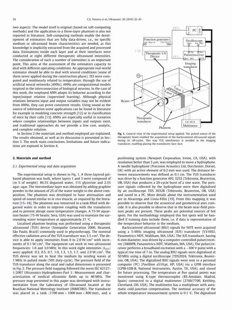
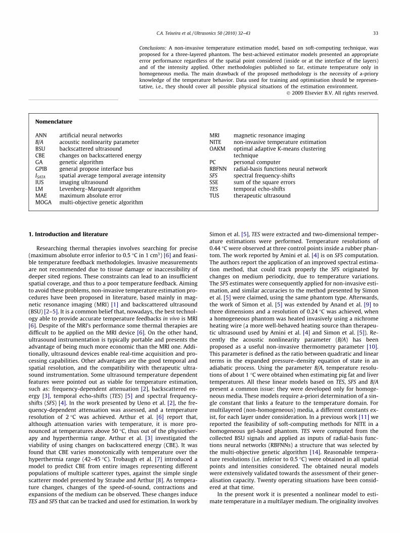
Fig. 1. General view of the experimental setup applied. The pulsed nature of thetherapeutic beam enabled the acquisition of the backscattered ultrasound signalsduring its off-cycles. This way TUS interference is avoided in the imagingtransducer, enabling placing the transducers face–face.

34 C.A. Teixeira et al. / Ultrasonics 50 (2010) 32–43

two aspects: The model itself is original (based on soft-computingmethods) and the application to a three-layer phantom is also notreported in literature. Soft-computing methods enable the devel-opment of estimators that are fully data-driven, i.e., no specificmedium or ultrasound beam characteristics are needed, as thisknowledge is implicitly extracted from the acquired and processeddata. Estimations inside each layer and at their interfaces wereconducted at eight different therapeutic ultrasound intensities.The consideration of such a number of intensities is an importantpoint. This aims at the assessment of the estimators capacity todeal with different operating conditions. An appropriate real-worldestimator should be able to deal with several conditions (some ofthem never applied during the construction phase). TES were com-puted and nonlinearly related to temperature, through the use ofartificial neural networks (ANNs). ANNs are computational modelsinspired in the interconnection of biological neurons. In the case ofthis work, the employed ANN adapts its behavior according to theinput/output relation (supervised learning). Although physicalrelations between input and output variables may not be evidentfrom ANNs, they can prove consistent results. Using sound as thesource of information some applications can be found in literaturefor example in modeling concrete strength [12] or in classificationof mice by their calls [13]. ANNs are especially useful in scenarioswhere complex relationships between inputs and outputs exist,and traditional approaches do not provide a low cost, analytic,and complete solution.

In Section 2 the materials and method employed are explained.The results obtained, as well as its discussion is presented in Sec-tion 3. The work main conclusions, limitations and future indica-tions are exposed in Section 4.

2. Materials and method

2.1. Experimental setup and data acquisition

The experimental setup is shown in Fig. 1. A three-layered gel-based phantom was built, where layers 1 and 3 were composed of(in % of weight): 86.5% degassed water, 11% glycerine and 2.5%agar–agar. The intermediate layer was obtained by adding graphitepowder in the amount of 2% of the water weight to the above com-position. The phantom was developed to have attenuation andspeed-of-sound similar to in vivo muscle, as required by the litera-ture [15–18]. The phantom was immersed in a tank filled with de-gassed water in order to improve coupling with the transducersand to prevent abrupt room temperature changes. A 75-W aquar-ium heater (75-W heater, Sera, USA) was used to maintain the sur-rounding water temperature at approximately 21 �C.

Localised phantom heating was performed using a therapeuticultrasound (TUS) device (Sonopulse Generation 2000, Ibramed,São Paulo, Brazil) commonly used in physiotherapy. The nominaleffective radiation area of the TUS transducer was 3:5 cm2. The de-vice is able to apply intensities from 0 to 2:0 W=cm2 with incre-ments of 0:1 W=cm2. The equipment can work in two ultrasoundfrequencies: 1.0 and 3.0 MHz. In this work eight intensities ðISATAÞwere applied: 0.3, 0.5, 0.7, 1.0, 1.3, 1.5, 1.7, and 2:0 W=cm2. TheTUS device was set to heat the medium by sending waves at1 MHz in pulsed mode (50% duty-cycle). The pressure field of theTUS transducer along the axial and radial dimensions is presentedin Fig. 2. The pressure field mapping followed the norm IEC 62127-1:2007 Ultrasonics-Hydrophones-Part 1: Measurement and char-acterization of medical ultrasonic fields up to 40 MHz. Thepressure map presented in this paper was developed with instru-mentation from the Laboratory of Ultrasound located at theBrazilian National Metrology Institute (INMETRO). The transducerwas placed in a tank ð1700 mm� 1000 mm� 800 mmÞ, and a

positioning system (Newport Corporation, Irvine, CA, USA), withresolution better than 5 lm, was employed to move a hydrophone.A needle hydrophone (Precision Acoustics Ltd, Dorchester, Dorset,UK) with an active element of 0.2 mm was used. The distance be-tween measurements was defined as 0.1 cm. The TUS transducerwas drive by a function generator AFG 3252 (Tektronix, Beaverton,OR, USA) that produces a 20-cycle burst of a sine wave. The pres-sure signals collected by the hydrophone were then digitalisedby an oscilloscope TDS 3032B (Tektronix, Beaverton, OR, USA)and saved in a PC. More details about the instrumentation usedare in Alvarenga and Costa-Félix [19]. From this mapping it waspossible to observe that the acoustical and geometrical axes coin-cide. It is also possible to observe that in the beam near-field pres-sure peaks are present. These peaks are potential sources of hotspots. For the methodology employed this hot spots will be han-dled if training data include them, i.e. if data is representative ofthe temperature behavior in the medium.

Backscattered ultrasound (BSU) signals for NITE were acquiredusing a 5-MHz imaging ultrasound (IUS) transducer (V310SU,Panametrics-NDT, Waltham, MA, USA). The IUS transducer, having6-mm diameter, was driven by a computer-controlled pulser/recei-ver (5800PR, Panametrics-NDT, Waltham, MA, USA). The pulser/re-ceiver performs a broadband excitation with a �300 V pulse with atypical rise time of 7 ns. The analog BSU signals were digitalised at50 MHz using a digital oscilloscope (TDS2024, Tektronix, Beaver-ton, OR, USA). The digitalised BSU signals were sent to a personalcomputer (PC) (Pavillion a510.pt, HP, USA) via a GPIB interface(GPIB-USB-B, National Instruments, Austin, TX, USA), and storedfor future processing. The temperature at five spatial points wasmonitored using K-type thermocouples (RS-Amidate, Madrid,Spain) connected to a digital multimeter (2700/7700, Keithley,Cleveland, OH, USA). The multimeter has a multiplexer with auto-matic cold-junction compensation. The nominal accuracy of thewhole temperature measurement system is 0.1 �C. The digitalised

020

4060

80100

120140

160180 −30

−20−10

010

2030

02468

1012141618

Radial Distance (mm)Axial Distance (mm)

Aco

usti

c P

ress

ure

(kP

a)

Fig. 2. Pressure field originated by the therapeutic transducer along the axial and radial dimensions. The pressure field was measured using calibrated instrumentation at theInstituto Nacional de Metrologia, Normalização e Qualidade Insdustrial (INMETRO), Rio de Janeiro, Brazil.

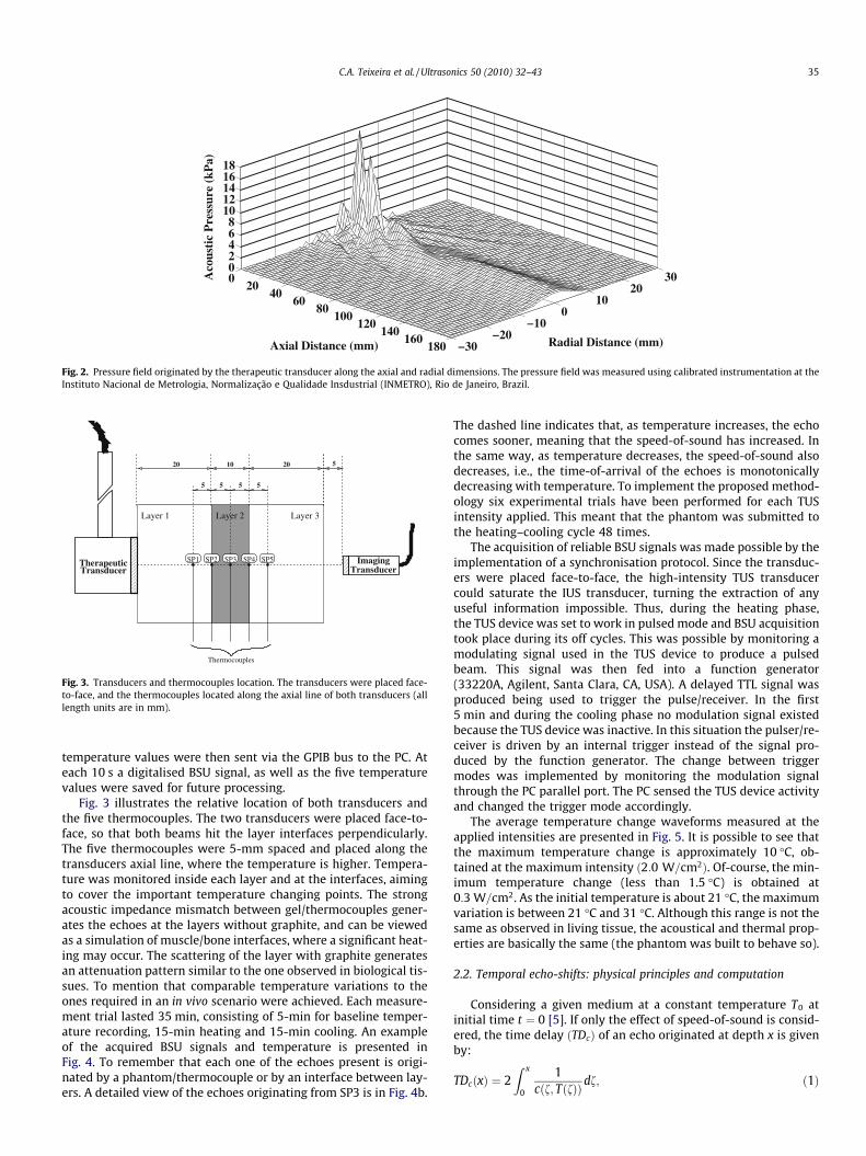
Fig. 3. Transducers and thermocouples location. The transducers were placed face-to-face, and the thermocouples located along the axial line of both transducers (alllength units are in mm).

C.A. Teixeira et al. / Ultrasonics 50 (2010) 32–43 35

temperature values were then sent via the GPIB bus to the PC. Ateach 10 s a digitalised BSU signal, as well as the five temperaturevalues were saved for future processing.

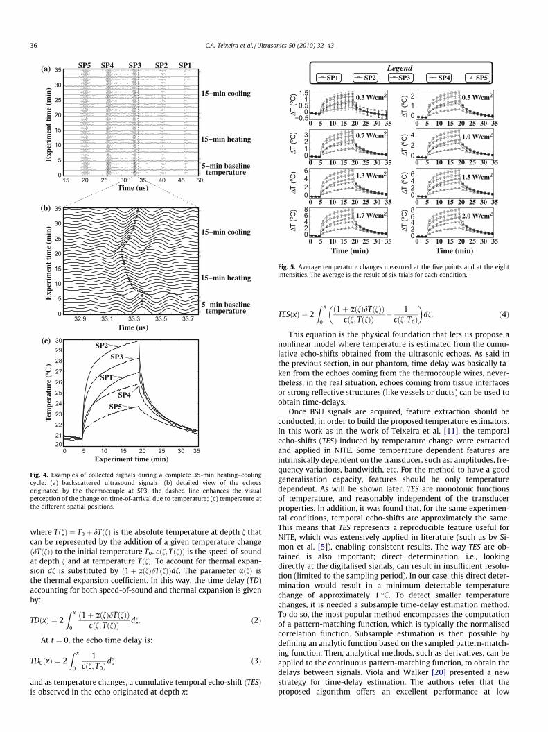
Fig. 3 illustrates the relative location of both transducers andthe five thermocouples. The two transducers were placed face-to-face, so that both beams hit the layer interfaces perpendicularly.The five thermocouples were 5-mm spaced and placed along thetransducers axial line, where the temperature is higher. Tempera-ture was monitored inside each layer and at the interfaces, aimingto cover the important temperature changing points. The strongacoustic impedance mismatch between gel/thermocouples gener-ates the echoes at the layers without graphite, and can be viewedas a simulation of muscle/bone interfaces, where a significant heat-ing may occur. The scattering of the layer with graphite generatesan attenuation pattern similar to the one observed in biological tis-sues. To mention that comparable temperature variations to theones required in an in vivo scenario were achieved. Each measure-ment trial lasted 35 min, consisting of 5-min for baseline temper-ature recording, 15-min heating and 15-min cooling. An exampleof the acquired BSU signals and temperature is presented inFig. 4. To remember that each one of the echoes present is origi-nated by a phantom/thermocouple or by an interface between lay-ers. A detailed view of the echoes originating from SP3 is in Fig. 4b.

The dashed line indicates that, as temperature increases, the echocomes sooner, meaning that the speed-of-sound has increased. Inthe same way, as temperature decreases, the speed-of-sound alsodecreases, i.e., the time-of-arrival of the echoes is monotonicallydecreasing with temperature. To implement the proposed method-ology six experimental trials have been performed for each TUSintensity applied. This meant that the phantom was submitted tothe heating–cooling cycle 48 times.

The acquisition of reliable BSU signals was made possible by theimplementation of a synchronisation protocol. Since the transduc-ers were placed face-to-face, the high-intensity TUS transducercould saturate the IUS transducer, turning the extraction of anyuseful information impossible. Thus, during the heating phase,the TUS device was set to work in pulsed mode and BSU acquisitiontook place during its off cycles. This was possible by monitoring amodulating signal used in the TUS device to produce a pulsedbeam. This signal was then fed into a function generator(33220A, Agilent, Santa Clara, CA, USA). A delayed TTL signal wasproduced being used to trigger the pulse/receiver. In the first5 min and during the cooling phase no modulation signal existedbecause the TUS device was inactive. In this situation the pulser/re-ceiver is driven by an internal trigger instead of the signal pro-duced by the function generator. The change between triggermodes was implemented by monitoring the modulation signalthrough the PC parallel port. The PC sensed the TUS device activityand changed the trigger mode accordingly.

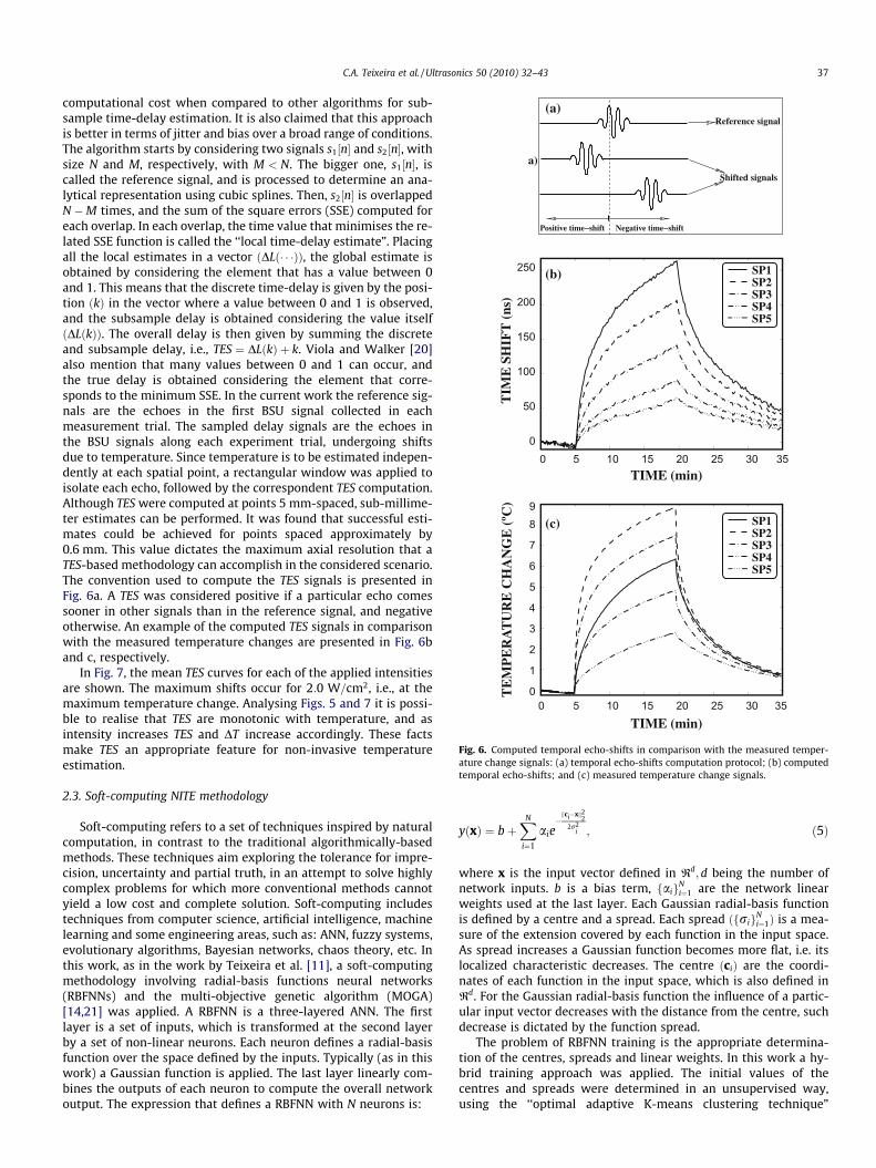
The average temperature change waveforms measured at theapplied intensities are presented in Fig. 5. It is possible to see thatthe maximum temperature change is approximately 10 �C, ob-tained at the maximum intensity ð2:0 W=cm2Þ. Of-course, the min-imum temperature change (less than 1.5 �C) is obtained at0:3 W=cm2. As the initial temperature is about 21 �C, the maximumvariation is between 21 �C and 31 �C. Although this range is not thesame as observed in living tissue, the acoustical and thermal prop-erties are basically the same (the phantom was built to behave so).

2.2. Temporal echo-shifts: physical principles and computation

Considering a given medium at a constant temperature T0 atinitial time t ¼ 0 [5]. If only the effect of speed-of-sound is consid-ered, the time delay ðTDcÞ of an echo originated at depth x is givenby:

TDcðxÞ ¼ 2Z x

0

1cðf; TðfÞÞ df; ð1Þ

15

0

20

5

32.9

25

10

30

15

33.1

35

20

40

25

33.3

45

30

50

35

33.5

0

20

0

5

21

33.7

5

10

22

10

15

23

15

20

24

20

25

25

25

30

26

30

35

27

35

28

2930

5−min baselinetemperature

15−min heating

15−min cooling

Time (us)

SP5(a)

SP2

SP3

SP1

SP4

SP5

(c)

5−min baselinetemperature

Time (us)

(b)

15−min heating

15−min cooling

Exp

erim

ent

tim

e (m

in)

Experiment time (min)

Tem

pera

ture

(ºC

)E

xper

imen

t ti

me

(min

)

SP1SP2SP3SP4

Fig. 4. Examples of collected signals during a complete 35-min heating–coolingcycle: (a) backscattered ultrasound signals; (b) detailed view of the echoesoriginated by the thermocouple at SP3, the dashed line enhances the visualperception of the change on time-of-arrival due to temperature; (c) temperature atthe different spatial positions.

5 10 15 20 25 30 350

5 10 15 20 25 30 3500

5 10 15 20 25 30 350

5 10 15 20 25 30 350

5 10 15 20 25 30 350

5 10 15 20 25 30 350

5 10 15 20 25 30 350

5 10 15 20 25 30 350

2

2

2

2

2

2

2

2

−0.5

0.51

1.5

3210

6420

86420 0

2468

0246

024

012

0

0.3 W/cm

0.7 W/cm

1.3 W/cm

1.7 W/cm

0.5 W/cm

1.0 W/cm

1.5 W/cm

2.0 W/cm

SP1 SP5SP3 SP4Legend

SP2

ΔΔ

ΔΔ Δ

ΔΔ

Δ

T (º

C)

T (º

C)

T (º

C)

T (º

C)

T (º

C)

T (º

C)

T (º

C)

T (º

C)

Time (min) Time (min)

Fig. 5. Average temperature changes measured at the five points and at the eightintensities. The average is the result of six trials for each condition.

36 C.A. Teixeira et al. / Ultrasonics 50 (2010) 32–43

where TðfÞ ¼ T0 þ dTðfÞ is the absolute temperature at depth f thatcan be represented by the addition of a given temperature changeðdTðfÞÞ to the initial temperature T0. cðf; TðfÞÞ is the speed-of-soundat depth f and at temperature TðfÞ. To account for thermal expan-sion df is substituted by ð1þ aðfÞdTðfÞÞdf. The parameter aðfÞ isthe thermal expansion coefficient. In this way, the time delay (TD)accounting for both speed-of-sound and thermal expansion is givenby:

TDðxÞ ¼ 2Z x

0

ð1þ aðfÞdTðfÞÞcðf; TðfÞÞ df: ð2Þ

At t ¼ 0, the echo time delay is:

TD0ðxÞ ¼ 2Z x

0

1cðf; T0Þ

df; ð3Þ

and as temperature changes, a cumulative temporal echo-shift ðTESÞis observed in the echo originated at depth x:

TESðxÞ ¼ 2Z x

0

ð1þ aðfÞdTðfÞÞcðf; TðfÞÞ � 1

cðf; T0Þ

� �df: ð4Þ

This equation is the physical foundation that lets us propose anonlinear model where temperature is estimated from the cumu-lative echo-shifts obtained from the ultrasonic echoes. As said inthe previous section, in our phantom, time-delay was basically ta-ken from the echoes coming from the thermocouple wires, never-theless, in the real situation, echoes coming from tissue interfacesor strong reflective structures (like vessels or ducts) can be used toobtain time-delays.

Once BSU signals are acquired, feature extraction should beconducted, in order to build the proposed temperature estimators.In this work as in the work of Teixeira et al. [11], the temporalecho-shifts (TES) induced by temperature change were extractedand applied in NITE. Some temperature dependent features areintrinsically dependent on the transducer, such as: amplitudes, fre-quency variations, bandwidth, etc. For the method to have a goodgeneralisation capacity, features should be only temperaturedependent. As will be shown later, TES are monotonic functionsof temperature, and reasonably independent of the transducerproperties. In addition, it was found that, for the same experimen-tal conditions, temporal echo-shifts are approximately the same.This means that TES represents a reproducible feature useful forNITE, which was extensively applied in literature (such as by Si-mon et al. [5]), enabling consistent results. The way TES are ob-tained is also important; direct determination, i.e., lookingdirectly at the digitalised signals, can result in insufficient resolu-tion (limited to the sampling period). In our case, this direct deter-mination would result in a minimum detectable temperaturechange of approximately 1 �C. To detect smaller temperaturechanges, it is needed a subsample time-delay estimation method.To do so, the most popular method encompasses the computationof a pattern-matching function, which is typically the normalisedcorrelation function. Subsample estimation is then possible bydefining an analytic function based on the sampled pattern-match-ing function. Then, analytical methods, such as derivatives, can beapplied to the continuous pattern-matching function, to obtain thedelays between signals. Viola and Walker [20] presented a newstrategy for time-delay estimation. The authors refer that theproposed algorithm offers an excellent performance at low

0

0

5

5

10

10

15

15

20

20

25

25

30

30

35

350

0

50

1

100

2

150

3

200

4

250

5

6

7

89

SP1

SP4SP5

SP3SP2

TIME (min)

SP1

SP4SP5

SP3SP2

TIME (min)

(a)

(b)

(c)

TIM

E S

HIF

T (

ns)

TE

MP

ER

AT

UR

E C

HA

NG

E (

ºC)

a)

Negative time−shiftPositive time−shift

Reference signal

Shifted signals

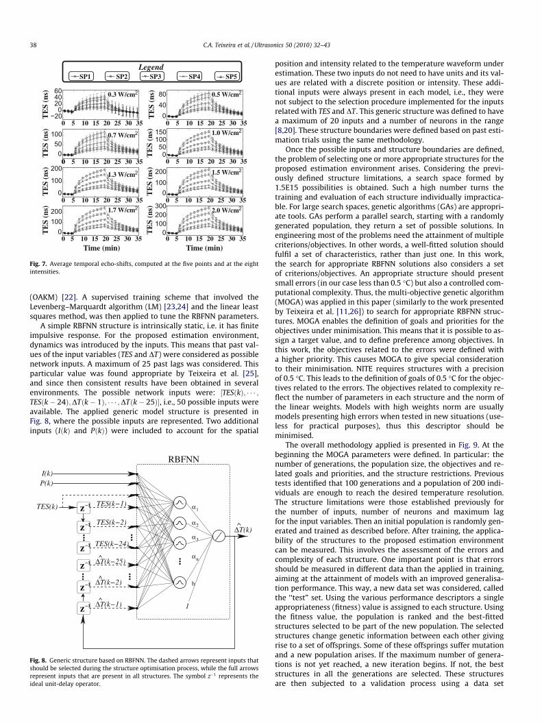
Fig. 6. Computed temporal echo-shifts in comparison with the measured temper-ature change signals: (a) temporal echo-shifts computation protocol; (b) computedtemporal echo-shifts; and (c) measured temperature change signals.

C.A. Teixeira et al. / Ultrasonics 50 (2010) 32–43 37

computational cost when compared to other algorithms for sub-sample time-delay estimation. It is also claimed that this approachis better in terms of jitter and bias over a broad range of conditions.The algorithm starts by considering two signals s1½n� and s2½n�, withsize N and M, respectively, with M < N. The bigger one, s1½n�, iscalled the reference signal, and is processed to determine an ana-lytical representation using cubic splines. Then, s2½n� is overlappedN �M times, and the sum of the square errors (SSE) computed foreach overlap. In each overlap, the time value that minimises the re-lated SSE function is called the ‘‘local time-delay estimate”. Placingall the local estimates in a vector ðDLð� � �ÞÞ, the global estimate isobtained by considering the element that has a value between 0and 1. This means that the discrete time-delay is given by the posi-tion ðkÞ in the vector where a value between 0 and 1 is observed,and the subsample delay is obtained considering the value itselfðDLðkÞÞ. The overall delay is then given by summing the discreteand subsample delay, i.e., TES ¼ DLðkÞ þ k. Viola and Walker [20]also mention that many values between 0 and 1 can occur, andthe true delay is obtained considering the element that corre-sponds to the minimum SSE. In the current work the reference sig-nals are the echoes in the first BSU signal collected in eachmeasurement trial. The sampled delay signals are the echoes inthe BSU signals along each experiment trial, undergoing shiftsdue to temperature. Since temperature is to be estimated indepen-dently at each spatial point, a rectangular window was applied toisolate each echo, followed by the correspondent TES computation.Although TES were computed at points 5 mm-spaced, sub-millime-ter estimates can be performed. It was found that successful esti-mates could be achieved for points spaced approximately by0.6 mm. This value dictates the maximum axial resolution that aTES-based methodology can accomplish in the considered scenario.The convention used to compute the TES signals is presented inFig. 6a. A TES was considered positive if a particular echo comessooner in other signals than in the reference signal, and negativeotherwise. An example of the computed TES signals in comparisonwith the measured temperature changes are presented in Fig. 6band c, respectively.

In Fig. 7, the mean TES curves for each of the applied intensitiesare shown. The maximum shifts occur for 2:0 W=cm2, i.e., at themaximum temperature change. Analysing Figs. 5 and 7 it is possi-ble to realise that TES are monotonic with temperature, and asintensity increases TES and DT increase accordingly. These factsmake TES an appropriate feature for non-invasive temperatureestimation.

2.3. Soft-computing NITE methodology

Soft-computing refers to a set of techniques inspired by naturalcomputation, in contrast to the traditional algorithmically-basedmethods. These techniques aim exploring the tolerance for impre-cision, uncertainty and partial truth, in an attempt to solve highlycomplex problems for which more conventional methods cannotyield a low cost and complete solution. Soft-computing includestechniques from computer science, artificial intelligence, machinelearning and some engineering areas, such as: ANN, fuzzy systems,evolutionary algorithms, Bayesian networks, chaos theory, etc. Inthis work, as in the work by Teixeira et al. [11], a soft-computingmethodology involving radial-basis functions neural networks(RBFNNs) and the multi-objective genetic algorithm (MOGA)[14,21] was applied. A RBFNN is a three-layered ANN. The firstlayer is a set of inputs, which is transformed at the second layerby a set of non-linear neurons. Each neuron defines a radial-basisfunction over the space defined by the inputs. Typically (as in thiswork) a Gaussian function is applied. The last layer linearly com-bines the outputs of each neuron to compute the overall networkoutput. The expression that defines a RBFNN with N neurons is:

yðxÞ ¼ bþXN

i¼1

aie�kci�xk2

22r2

i ; ð5Þ

where x is the input vector defined in Rd;d being the number ofnetwork inputs. b is a bias term, faigN

i¼1 are the network linearweights used at the last layer. Each Gaussian radial-basis functionis defined by a centre and a spread. Each spread ðfrigN

i¼1Þ is a mea-sure of the extension covered by each function in the input space.As spread increases a Gaussian function becomes more flat, i.e. itslocalized characteristic decreases. The centre ðciÞ are the coordi-nates of each function in the input space, which is also defined inRd. For the Gaussian radial-basis function the influence of a partic-ular input vector decreases with the distance from the centre, suchdecrease is dictated by the function spread.

The problem of RBFNN training is the appropriate determina-tion of the centres, spreads and linear weights. In this work a hy-brid training approach was applied. The initial values of thecentres and spreads were determined in an unsupervised way,using the ‘‘optimal adaptive K-means clustering technique”

5 10 15 20 25 30 350

5 10 15 20 25 30 3500

5 10 15 20 25 30 350

5 10 15 20 25 30 350

5 10 15 20 25 30 350

5 10 15 20 25 30 350

5 10 15 20 25 30 3505 10 15 20 25 30 350

2

2

2

2

2

2

2

2

0.7 W/cm

1.3 W/cm

SP1 SP5SP3 SP4Legend

SP2

1.7 W/cm

0.5 W/cm

1.0 W/cm

1.5 W/cm

2.0 W/cm

0.3 W/cm

TE

S (n

s)T

ES

(ns)

TE

S (n

s)T

ES

(ns)

TE

S (n

s)T

ES

(ns)

TE

S (n

s)T

ES

(ns)

Time (min)Time (min)

0100200

0100200300

0100200

050

100150

04080

−200

204060

100500

200

100

0

Fig. 7. Average temporal echo-shifts, computed at the five points and at the eightintensities.

38 C.A. Teixeira et al. / Ultrasonics 50 (2010) 32–43

(OAKM) [22]. A supervised training scheme that involved theLevenberg–Marquardt algorithm (LM) [23,24] and the linear leastsquares method, was then applied to tune the RBFNN parameters.

A simple RBFNN structure is intrinsically static, i.e. it has finiteimpulsive response. For the proposed estimation environment,dynamics was introduced by the inputs. This means that past val-ues of the input variables (TES and DT) were considered as possiblenetwork inputs. A maximum of 25 past lags was considered. Thisparticular value was found appropriate by Teixeira et al. [25],and since then consistent results have been obtained in severalenvironments. The possible network inputs were: ½TESðkÞ; � � � ;TESðk� 24Þ;DTðk� 1Þ; � � � ;DTðk� 25Þ�, i.e., 50 possible inputs wereavailable. The applied generic model structure is presented inFig. 8, where the possible inputs are represented. Two additionalinputs (IðkÞ and PðkÞ) were included to account for the spatial

Fig. 8. Generic structure based on RBFNN. The dashed arrows represent inputs thatshould be selected during the structure optimisation process, while the full arrowsrepresent inputs that are present in all structures. The symbol z�1 represents theideal unit-delay operator.

position and intensity related to the temperature waveform underestimation. These two inputs do not need to have units and its val-ues are related with a discrete position or intensity. These addi-tional inputs were always present in each model, i.e., they werenot subject to the selection procedure implemented for the inputsrelated with TES and DT . This generic structure was defined to havea maximum of 20 inputs and a number of neurons in the range[8,20]. These structure boundaries were defined based on past esti-mation trials using the same methodology.

Once the possible inputs and structure boundaries are defined,the problem of selecting one or more appropriate structures for theproposed estimation environment arises. Considering the previ-ously defined structure limitations, a search space formed by1.5E15 possibilities is obtained. Such a high number turns thetraining and evaluation of each structure individually impractica-ble. For large search spaces, genetic algorithms (GAs) are appropri-ate tools. GAs perform a parallel search, starting with a randomlygenerated population, they return a set of possible solutions. Inengineering most of the problems need the attainment of multiplecriterions/objectives. In other words, a well-fitted solution shouldfulfil a set of characteristics, rather than just one. In this work,the search for appropriate RBFNN solutions also considers a setof criterions/objectives. An appropriate structure should presentsmall errors (in our case less than 0.5 �C) but also a controlled com-putational complexity. Thus, the multi-objective genetic algorithm(MOGA) was applied in this paper (similarly to the work presentedby Teixeira et al. [11,26]) to search for appropriate RBFNN struc-tures. MOGA enables the definition of goals and priorities for theobjectives under minimisation. This means that it is possible to as-sign a target value, and to define preference among objectives. Inthis work, the objectives related to the errors were defined witha higher priority. This causes MOGA to give special considerationto their minimisation. NITE requires structures with a precisionof 0.5 �C. This leads to the definition of goals of 0.5 �C for the objec-tives related to the errors. The objectives related to complexity re-flect the number of parameters in each structure and the norm ofthe linear weights. Models with high weights norm are usuallymodels presenting high errors when tested in new situations (use-less for practical purposes), thus this descriptor should beminimised.

The overall methodology applied is presented in Fig. 9. At thebeginning the MOGA parameters were defined. In particular: thenumber of generations, the population size, the objectives and re-lated goals and priorities, and the structure restrictions. Previoustests identified that 100 generations and a population of 200 indi-viduals are enough to reach the desired temperature resolution.The structure limitations were those established previously forthe number of inputs, number of neurons and maximum lagfor the input variables. Then an initial population is randomly gen-erated and trained as described before. After training, the applica-bility of the structures to the proposed estimation environmentcan be measured. This involves the assessment of the errors andcomplexity of each structure. One important point is that errorsshould be measured in different data than the applied in training,aiming at the attainment of models with an improved generalisa-tion performance. This way, a new data set was considered, calledthe ‘‘test” set. Using the various performance descriptors a singleappropriateness (fitness) value is assigned to each structure. Usingthe fitness value, the population is ranked and the best-fittedstructures selected to be part of the new population. The selectedstructures change genetic information between each other givingrise to a set of offsprings. Some of these offsprings suffer mutationand a new population arises. If the maximum number of genera-tions is not yet reached, a new iteration begins. If not, the beststructures in all the generations are selected. These structuresare then subjected to a validation process using a data set

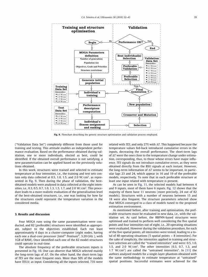
Fig. 9. Flowchart describing the generic structure optimisation and validation process employed.

C.A. Teixeira et al. / Ultrasonics 50 (2010) 32–43 39

(‘‘Validation Data Set”) completely different from those used fortraining and testing. This attitude enables an independent perfor-mance evaluation. Based on the performance obtained during val-idation, one or more individuals, elected as best, could beidentified. If the obtained overall performance is not satisfying, anew parametrisation can be applied based on the previously solu-tions obtained.

In this work, structures were trained and selected to estimatetemperature at four intensities, i.e., the training and test sets con-tain only data collected at 0.5, 1.0, 1.5, and 2:0 W=cm2, as repre-sented in Fig. 9. Then during the phase of validation, the best-obtained models were analysed in data collected at the eight inten-sities, i.e., 0.3, 0.5, 0.7, 1.0, 1.3, 1.5, 1.7, and 2:0 W=cm2. This proce-dure leads to a more realistic evaluation of the generalisation levelof the best-obtained structures, i.e., one was looking for how farthe structures could represent the temperature variation in theconsidered media.

3. Results and discussion

Four MOGA runs using the same parametrisation were con-ducted, and 82 (preferable) structures were identified as appropri-ate, subject to the objectives established. Each run leastapproximately 4 days in a cluster-computer (eight nodes, havingeach one a dual-core processor (Intel� Pentium�, 3.20 GHz ), with1GB of RAM). Once identified each one of the 82 model structurescould operate in real-time.

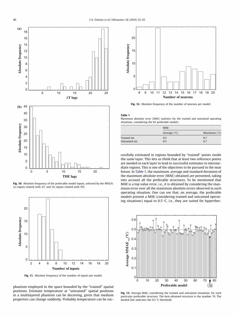
The absolute frequency of the preferable structures inputs ispresented in Fig. 10. One can observe that MOGA selected mainlythe long-term lags of DT . On the other hand, the short-term lagsof TES are the most frequent ones. More than 50% of the modelshave TESðkÞ as input. Considering all the inputs selected, 73% were

related with TES, and only 27% with DT . This happened because thetemperature values fed-back introduced cumulative errors in theinputs, decreasing the overall performance. The short-term lagsof DT were the ones close to the temperature change under estima-tion, corresponding, thus, to those whose errors have major influ-ence. TES signals do not introduce cumulative errors, as they wereobtained directly from the BSU signals at each instant. However,the long-term information of DT seems to be important, in partic-ular lags 23 and 24, which appear in 16 and 19 of the preferablemodels, respectively. To note that in each preferable structure atleast one input related with temperature is present.

As can be seen in Fig. 11, the selected models had between 4and 9 inputs, most of them have 6 inputs. Fig. 12 shows that themajority of them have 11 neurons (more precisely, 24 out of 82models). Structures with a number of neurons between 15 and18 were also frequent. The structure parameters selected showthat MOGA converged to a class of models tuned to the proposedestimation environment.

As mentioned before, after training and optimisation, the pref-erable structures must be evaluated in new data, i.e., with the val-idation set. As said before, the RBFNN-based structures wereoptimised and trained to perform well considering the five spatialpoints and four intensities out of eight, i.e., 20 operating situationswere evaluated. However during the validation procedure, for eachof the five spatial points, all intensities were tested, leading to a to-tal of 40 operating situations (5 spatial points � 8 intensities). Forthe sake of simplicity, the intensities applied in training and struc-ture selection are called the ‘‘trained intensities” and were: 0.5, 1.0,1.5, and 2:0 W=cm2. The other intensities (0.3, 0.7, 1.3, and1:7 W=cm2) are called the ‘‘untrained intensities”. In [11] theauthors analysed models for a single-layer phantom obtained withthe same methodology to estimate temperature at ‘‘untrained”spatial positions. Successful estimates were achieved for the

5 10 15 20 25

0 5 10 15 200

5

10

15

20

25

30

35

40

45

0

2

4

6

8

10

12

14

16

18

ΔT lags

TDE lags

(a)

(b)

Abs

olut

e fr

eque

ncy

Abs

olut

e fr

eque

ncy

Fig. 10. Absolute frequency of the preferable model inputs, selected by the MOGA:(a) inputs related with DT , and (b) inputs related with TES.

2 4 6 8 10 12 14 16 18 200

5

10

15

20

Number of inputs

Abs

olut

e fr

eque

ncy

Fig. 11. Absolute frequency of the number of inputs per model.

8 9 10 11 12 13 14 15 160

17

5

18

10

19

15

20

20

Number of neurons

Abs

olut

e fr

eque

ncy

Fig. 12. Absolute frequency of the number of neurons per model.

Table 1Maximum absolute error (MAE) statistics for the trained and untrained operatingsituations, considering the 82 preferable models.

MAE

Average (�C) Maximum (�C)

Trained int. 0.5 0.7Untrained int. 0.5 0.7

0

0.1

0.2

0.3

0.4

0.5

0.6

0 10 20 30 40 50 60 70 8076Preferable model

Ave

rage

MM

AE

(

ºC)

VL

Fig. 13. Average MAE, considering the trained and untrained situations, for eachparticular preferable structure. The best-obtained structure is the number 76. Thedashed line indicates the 0.5 �C threshold.

40 C.A. Teixeira et al. / Ultrasonics 50 (2010) 32–43

phantom employed in the space bounded by the ‘‘trained” spatialpositions. Estimate temperature at ‘‘untrained” spatial positionsin a multilayered phantom can be deceiving, given that mediumproperties can change suddenly. Probably temperature can be suc-

cessfully estimated in regions bounded by ‘‘trained” points insidethe same layer. This lets us think that at least two reference pointsare needed in each layer to lead to successful estimates in interme-diate regions. This is one of the objectives to be pursued in the nearfuture. In Table 1, the maximum, average and standard deviation ofthe maximum absolute error (MAE) obtained are presented, takinginto account all the preferable structures. To be mentioned thatMAE is a top value error, i.e., it is obtained by considering the max-imum error over all the maximum absolute errors observed in eachoperating situation. One can see that, on average, the preferablemodels present a MAE (considering trained and untrained operat-ing situations) equal to 0.5 �C, i.e., they are suited for hyperther-

T (

ºC)

Δ T (

ºC)

Δ

5 10 15 20 25 30 35

T (

ºC)

Δ

5 10 15 20 25 30 35Experiment time (min)

5 10 15 20 25 30 35Experiment time (min)

T (

ºC)

Δ

0

0.5

1

1.5

2

2.5

0

0.5

1

1.5

2

2.5

3

3.5

4

4.55

5 10 15 20 25 30 35Experiment time (min)

0

1

2

3

4

5

6

7

8

Experiment time (min)

0

1

2

3

4

5

6

7

8

9

(b)(a)

(d)(c)

SP1

SP2

SP3

SP4

SP5

SP2

SP3

SP1

SP4

SP5

SP2

SP3

SP1

SP4

SP5

SP2

SP3

SP1

SP4

SP5

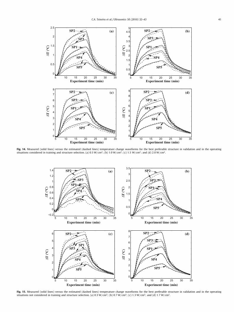
Fig. 14. Measured (solid lines) versus the estimated (dashed lines) temperature change waveforms for the best preferable structure in validation and in the operatingsituations considered in training and structure selection. (a) 0:5 W=cm2; (b) 1:0 W=cm2; (c) 1:5 W=cm2; and (d) 2:0 W=cm2.

Experiment time (min)

Experiment time (min)

Experiment time (min)

Experiment time (min)

(a)

(c)

(b)

(d)

SP2

SP3SP1

SP4

SP5

SP2

SP3

SP1

SP4

SP5

SP2

SP3SP1

SP4

SP5

SP2

SP3

SP1

SP4

SP5

Δ

ΔΔ

Δ T

(ºC

)

T (

ºC)

T (

ºC)

T (

ºC)

5 10 15 20 25 30 35

5 10 15 20 25 30 35

5 10 15 20 25 30 35

−0.2

0

0.2

0.4

0.6

0.8

1

1.2

1.4

0

0.5

1

1.5

2

2.5

3

3.5

0

1

2

3

4

5

6

0

1

2

3

4

5

6

7

8

5 10 15 20 25 30 35

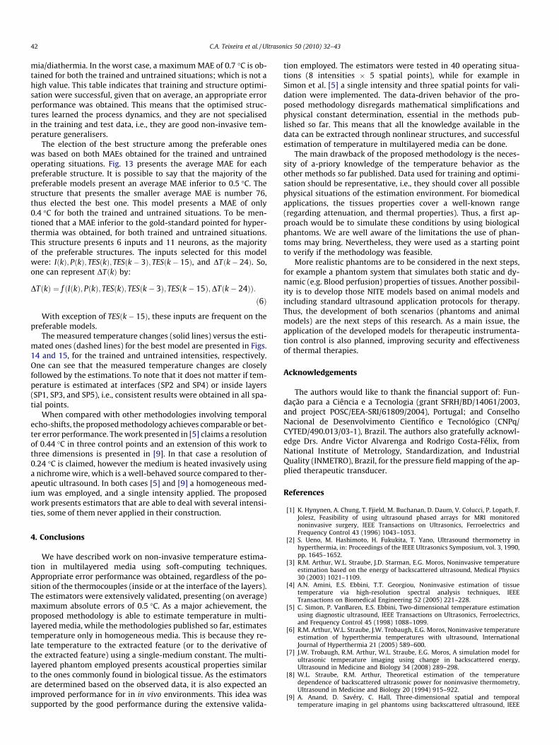
Fig. 15. Measured (solid lines) versus the estimated (dashed lines) temperature change waveforms for the best preferable structure in validation and in the operatingsituations not considered in training and structure selection. (a) 0:3 W=cm2; (b) 0:7 W=cm2; (c) 1:3 W=cm2; and (d) 1:7 W=cm2.

C.A. Teixeira et al. / Ultrasonics 50 (2010) 32–43 41

42 C.A. Teixeira et al. / Ultrasonics 50 (2010) 32–43

mia/diathermia. In the worst case, a maximum MAE of 0.7 �C is ob-tained for both the trained and untrained situations; which is not ahigh value. This table indicates that training and structure optimi-sation were successful, given that on average, an appropriate errorperformance was obtained. This means that the optimised struc-tures learned the process dynamics, and they are not specialisedin the training and test data, i.e., they are good non-invasive tem-perature generalisers.

The election of the best structure among the preferable oneswas based on both MAEs obtained for the trained and untrainedoperating situations. Fig. 13 presents the average MAE for eachpreferable structure. It is possible to say that the majority of thepreferable models present an average MAE inferior to 0.5 �C. Thestructure that presents the smaller average MAE is number 76,thus elected the best one. This model presents a MAE of only0.4 �C for both the trained and untrained situations. To be men-tioned that a MAE inferior to the gold-standard pointed for hyper-thermia was obtained, for both trained and untrained situations.This structure presents 6 inputs and 11 neurons, as the majorityof the preferable structures. The inputs selected for this modelwere: IðkÞ; PðkÞ; TESðkÞ; TESðk� 3Þ; TESðk� 15Þ, and DTðk� 24Þ. So,one can represent DTðkÞ by:

DTðkÞ ¼ f ðIðkÞ; PðkÞ; TESðkÞ; TESðk� 3Þ; TESðk� 15Þ;DTðk� 24ÞÞ:ð6Þ

With exception of TESðk� 15Þ, these inputs are frequent on thepreferable models.

The measured temperature changes (solid lines) versus the esti-mated ones (dashed lines) for the best model are presented in Figs.14 and 15, for the trained and untrained intensities, respectively.One can see that the measured temperature changes are closelyfollowed by the estimations. To note that it does not matter if tem-perature is estimated at interfaces (SP2 and SP4) or inside layers(SP1, SP3, and SP5), i.e., consistent results were obtained in all spa-tial points.

When compared with other methodologies involving temporalecho-shifts, the proposed methodology achieves comparable or bet-ter error performance. The work presented in [5] claims a resolutionof 0.44 �C in three control points and an extension of this work tothree dimensions is presented in [9]. In that case a resolution of0.24 �C is claimed, however the medium is heated invasively usinga nichrome wire, which is a well-behaved source compared to ther-apeutic ultrasound. In both cases [5] and [9] a homogeneous med-ium was employed, and a single intensity applied. The proposedwork presents estimators that are able to deal with several intensi-ties, some of them never applied in their construction.

4. Conclusions

We have described work on non-invasive temperature estima-tion in multilayered media using soft-computing techniques.Appropriate error performance was obtained, regardless of the po-sition of the thermocouples (inside or at the interface of the layers).The estimators were extensively validated, presenting (on average)maximum absolute errors of 0.5 �C. As a major achievement, theproposed methodology is able to estimate temperature in multi-layered media, while the methodologies published so far, estimatestemperature only in homogeneous media. This is because they re-late temperature to the extracted feature (or to the derivative ofthe extracted feature) using a single-medium constant. The multi-layered phantom employed presents acoustical properties similarto the ones commonly found in biological tissue. As the estimatorsare determined based on the observed data, it is also expected animproved performance for in in vivo environments. This idea wassupported by the good performance during the extensive valida-

tion employed. The estimators were tested in 40 operating situa-tions (8 intensities � 5 spatial points), while for example inSimon et al. [5] a single intensity and three spatial points for vali-dation were implemented. The data-driven behavior of the pro-posed methodology disregards mathematical simplifications andphysical constant determination, essential in the methods pub-lished so far. This means that all the knowledge available in thedata can be extracted through nonlinear structures, and successfulestimation of temperature in multilayered media can be done.

The main drawback of the proposed methodology is the neces-sity of a-priory knowledge of the temperature behavior as theother methods so far published. Data used for training and optimi-sation should be representative, i.e., they should cover all possiblephysical situations of the estimation environment. For biomedicalapplications, the tissues properties cover a well-known range(regarding attenuation, and thermal properties). Thus, a first ap-proach would be to simulate these conditions by using biologicalphantoms. We are well aware of the limitations the use of phan-toms may bring. Nevertheless, they were used as a starting pointto verify if the methodology was feasible.

More realistic phantoms are to be considered in the next steps,for example a phantom system that simulates both static and dy-namic (e.g. Blood perfusion) properties of tissues. Another possibil-ity is to develop those NITE models based on animal models andincluding standard ultrasound application protocols for therapy.Thus, the development of both scenarios (phantoms and animalmodels) are the next steps of this research. As a main issue, theapplication of the developed models for therapeutic instrumenta-tion control is also planned, improving security and effectivenessof thermal therapies.

Acknowledgements

The authors would like to thank the financial support of: Fun-dação para a Ciência e a Tecnologia (grant SFRH/BD/14061/2003,and project POSC/EEA-SRI/61809/2004), Portugal; and ConselhoNacional de Desenvolvimento Científico e Tecnológico (CNPq/CYTED/490.013/03-1), Brazil. The authors also gratefully acknowl-edge Drs. Andre Victor Alvarenga and Rodrigo Costa-Félix, fromNational Institute of Metrology, Standardization, and IndustrialQuality (INMETRO), Brazil, for the pressure field mapping of the ap-plied therapeutic transducer.

References

[1] K. Hynynen, A. Chung, T. Fjield, M. Buchanan, D. Daum, V. Colucci, P. Lopath, F.Jolesz, Feasibility of using ultrasound phased arrays for MRI monitorednoninvasive surgery, IEEE Transactions on Ultrasonics, Ferroelectrics andFrequency Control 43 (1996) 1043–1053.

[2] S. Ueno, M. Hashimoto, H. Fukukita, T. Yano, Ultrasound thermometry inhyperthermia, in: Proceedings of the IEEE Ultrasonics Symposium, vol. 3, 1990,pp. 1645–1652.

[3] R.M. Arthur, W.L. Straube, J.D. Starman, E.G. Moros, Noninvasive temperatureestimation based on the energy of backscattered ultrasound, Medical Physics30 (2003) 1021–1109.

[4] A.N. Amini, E.S. Ebbini, T.T. Georgiou, Noninvasive estimation of tissuetemperature via high-resolution spectral analysis techniques, IEEETransactions on Biomedical Engineering 52 (2005) 221–228.

[5] C. Simon, P. VanBaren, E.S. Ebbini, Two-dimensional temperature estimationusing diagnostic ultrasound, IEEE Transactions on Ultrasonics, Ferroelectrics,and Frequency Control 45 (1998) 1088–1099.

[6] R.M. Arthur, W.L. Straube, J.W. Trobaugh, E.G. Moros, Noninvasive temperatureestimation of hyperthermia temperatures with ultrasound, InternationalJournal of Hyperthermia 21 (2005) 589–600.

[7] J.W. Trobaugh, R.M. Arthur, W.L. Straube, E.G. Moros, A simulation model forultrasonic temperature imaging using change in backscattered energy,Ultrasound in Medicine and Biology 34 (2008) 289–298.

[8] W.L. Straube, R.M. Arthur, Theoretical estimation of the temperaturedependence of backscattered ultrasonic power for noninvasive thermometry,Ultrasound in Medicine and Biology 20 (1994) 915–922.

[9] A. Anand, D. Savéry, C. Hall, Three-dimensional spatial and temporaltemperature imaging in gel phantoms using backscattered ultrasound, IEEE

C.A. Teixeira et al. / Ultrasonics 50 (2010) 32–43 43

Transactions on Ultrasonics, Ferroelectrics, and Frequency Control 54 (2007)23–31.

[10] X. Liu, X. Gong, C. Yin, J. Li, D. Zhang, Noninvasive estimation of temperatureelevations in biological tissues using acoustic nonlinearity parameter imaging,Ultrasound in Medicine and Biology 34 (2008) 414–424.

[11] C.A. Teixeira, M.G. Ruano, A.E. Ruano, W.C.A. Pereira, A soft-computingmethodology for noninvasive time-spatial temperature estimation, IEEETransactions on Biomedical Engineering 22 (2008) 572–580.

[12] G. Trtnik, F. Kavcic, G. Turk, Prediction of concrete strength using ultrasonicpulse velocity and artificial neural networks, Ultrasonics 49 (2009) 53–60.

[13] H. Tian, Z. Shang, Artificial neural network as a classification method of miceby their calls, Ultrasonics 44 (2006) e275–e278.

[14] C. Fonseca, P. Fleming, Genetic algorithms for multi-objective optimization:Formulation, discussion and generalization, in: Proceedings of the 5thInternational Conference on Genetic Algorithms, 1993, 416–423.

[15] AIUM Technical Standards Committee, Methods For Specifying AcousticProperties of Tissue Mimicking Phantoms and Objects, American Institute ofUltrasound in Medicine, 1995.

[16] M.M. Burlew, E.L. Madsen, J.A. Zagzebski, R.A. Banjavie, S.W. Sum, A newultrasound tissue-equivalent material, Radiology 134 (1980) 517–520.

[17] E.L. Madsen, J.A. Zagzebski, R.A. Banjavie, R.E. Jutila, Tissue mimickingmaterials for ultrasound phantoms, Medical Physics 5 (1978) 391–394.

[18] S.Y. Sato, W.C.A. Pereira, C.R.S. Vieira, Phantom to measure displayed dynamicrange at biomedical ultrasound equipments, Brazilian Journal of BiomedicalEngineering 19 (2003) 157–166.

[19] A.V. Alvarenga, R.P.B. Costa-Félix, Uncertainty assessment of effectiveradiating area and beam non-uniformity ratio of ultrasound transducersdetermined according to IEC 61689:2007. Metrologia 46 (2009) 367–374.

[20] F. Viola, W.F. Walker, A spline-based algorithm for continuous time-delayestimation using sampled data, IEEE Transactions on Ultrasonics,Ferroelectrics, and Frequency Control 52 (2005) 80–93.

[21] C.M. Fonseca, P. Fleming, Multiobjective optimization and multiple constrainthandling with evolutionary algorithms – part i: a unified formulation, IEEETransactions on Systems, Man and Cybernetics Part A – Systems and Humans28 (1998) 26–37.

[22] C. Chinrungrueng, S.H. Séquin, Optimal adaptive k-means algorithm withdynamic adjustment of learning rate, IEEE Transactions on Neural Networks 6(1995) 157–169.

[23] D. Marquardt, An algorithm for least-squares estimation of nonlinearparameters, SIAM Journal of Applied Mathematics 11 (1963) 431–441.

[24] K. Levenberg, A method for the solution of certain problems in least squares,Quarterly Applied Mathematics 2 (1944) 164–168.

[25] C.A. Teixeira, M.G. Ruano, A.E. Ruano, W.C.A. Pereira, C. Negreira, Single black-box models for two-point non-invasive temperature prediction, in:Proceedings of the 6th IFAC Symposium on Modelling and Control inBiomedical Systems, Elsevier, 2006, pp. 135–140.

[26] C.A. Teixeira, A.E. Ruano, C. Negreira, M.G. Ruano, W.C.A. Pereira, Non-invasivetemperature prediction of in-vitro therapeutic ultrasound signals using neuralnetworks, Medical and Biological Engineering and Computing 44 (2006) 111–116.