�$����% �&�������� ��

������������������ ��������������������

����������������

������������ !��"��

���# �"�������'()*

����+,,!!!��-�����",������,!'()*

��� �����$������������� ��������

./*/������0���������1����

��2-� 3"�4����/).56

�����2-���)///

�������������������� �����������������������������������������������������������������������

����������������������� �������������������������������!�����������������������������"����#����

�������"�����$��������"���������"�����������#�#������������%"�������&���'��������'�����(����

���&������)���*�����������+������,�����$�������������������������������������������������������

��� ���� ������(������� ��&&���� ��&� �&���� ����������� ���-�����.���������-����������/�%$�

����&"���.�������������0�112�������%����&�������������3������������.�����������-���&������4��

������������������%����&��������.������������� ������������.5�3���������$�����-������

������������������$�����-�������3������������������$�����-������� ���6����)����������������

.������������������������3�3����.���������)�&������"���6������������ -%$���&&��4�������

����������������������������������������&����� ����������������������������������������� ����

�������������������������������������������������� ��������-��������%����&���$�����������

7�8999�"��$��������������������������(����������������������������������������������� ���������

� �������������������&���"��:��������������� ���������&����������������������������������������7

����������������������������

���������������7���� �����38���2���������

�������������������3������������� !��"��

�$�����# �"�����������'()*

�����2-���)///

��������

����������� �����������3 ���������������7�0�� �����38���2����������������9��1��������������� �3 ��0�

�7����0�����0�3���������� 2������������0����������2�������7���� 0�����0 7 0�� ����7�0�� �����38���2���

0������ ���77�0�4���������2������������� 2���:�0��������������3�0���������� ���������� ���� ��-��!���

�1���2������3����7 ��- � �:������!����0�1��� �����������9��1���3���������7 �3 �"�� �3 0����������

2�3���!� 0��2 ;���-����0��1�;���3����0��1�;��38���2����0�����! ��� ���1��� - � �:�7 �������3���

-����

���������������� ������������ !��"��

������2�����7��0���2 0� ������2�����7��0���2 0�

$�������� 1��� �: �� 1��� �:��7����:���3

)'/�$� �����"�����#4����)/'<)

$�����4����/)).* ��3��$�

��3��$� ����=0:0������23��3�

�0�����=-���3�

1 Motivation

The goal of this paper is to understand the nature of capital adjustmentcosts. This topic is central to the understanding of investment, one of themost important and volatile components of aggregate activity. Moreover,understanding of the nature of adjustment costs is vital for the evaluationof policies, such as tax credits, that attempt to influence investment andthus aggregate activity. Despite the obvious importance of investment tomacroeconomics, it remains an enigma.Costs of adjusting the stock of capital reflect a variety of interrelated

factors that are difficult to measure directly or precisely.1 Changing the levelof capital services at a business generates disruption costs during installationof any new or replacement capital and costly learning must be incurred as thestructure of production may have been changed. Installing new equipmentor structures often involves delivery lags and time to install and/or build.The irreversibility of many projects caused by a lack of secondary marketsfor capital goods acts as another form of adjustment cost.

Some industry case studies (e.g., Holt et al. [1960], Peck [1974], Ito,Bresnahan and Greenstein [1998]) provide a detailed characterization of thenature of the adjustment costs for specific technologies. A reading of theseindustry case studies suggest that there are indeed many different facets ofadjustment costs and that, in terms of modeling these adjustment costs, bothconvex and nonconvex elements are likely to be present.2

Despite this perspective from the industry case studies, the workhorsemodel of the investment literature has been a standard neoclassical model

1As direct measurement of these many factors is difficult, for the most part the studyof capital adjustment costs has been indirect through studying the dynamics of investmentitself.

2Holt et. al. [1960] found a quadratic specification of adjustment costs to be a goodapproximation of hiring and layoff costs, overtime costs, inventory costs and machinesetup costs in the selected manufacturing industries. These components of adjustmentcosts for changing the level of production are relevant here but are by no means the onlyrelevant costs. In terms of changes in the level of capital services, Peck [1974] studiesinvestment in turbogenerator sets for a panel of 15 electric utility firms and found that”The investments in turbogenerator sets undertaken by any firm took place at discrete andoften widely dispersed points of time.”In their study of investment in large scale computersystems, Ito, Bresnahan and Greenstein [1998] also find evidence of lumpy investment.Their analysis of the costs of adjusting the stock of computer capital include items whichthey term ”... intangible organization capital such as production knowledge and tacit workroutines.”

2

with convex costs (often approximated to be quadratic) of adjustment.3 Thismodel has not performed that well even at the aggregate level (see Caballero[1999]) but the recent development of longitudinal establishment databaseshas raised even more questions about the standard convex cost model.An alternative approach, highlighted in the work of Doms-Dunne [1994],

Cooper, Haltiwanger and Power [1999], Abel-Eberly [1994, 1996], and Ca-ballero, Engel and Haltiwanger [1995], argues that nonconvexities and irre-versibilities play a central role in the investment process. The primary basisfor this view, reviewed in detail below, is plant-level evidence of a nonlinearrelationship between investment and measures of fundamentals, includinginvestment bursts (spikes) as well as periods of inaction.One limitation of this recent empirical literature is that it has focused

primarily on reduced form implications of nonconvex vs. convex models.The results that emerge reject the reduced form implications of a pure convexmodel and are consistent with the presence of nonconvexities. The reducedform nature of the results have left us with several important, unresolvedquestions: what is the nature of the capital adjustment process at the microlevel? Does the micro evidence support the presence of both convex andnonconvex components of adjustment costs as might be expected based uponthe limited number of industry case studies? More specifically, what are thestructural estimates of the convex and nonconvex components of adjustmentcosts that are consistent with the micro evidence? Finally, what are theaggregate and policy implications of the estimated investment model?To address these questions, this paper considers a rich model of capital

adjustment which nests alternative specifications. To do so, we specify a dy-namic optimizing problem at the plant-level which incorporates both convexand nonconvex costs of adjustment as well as irreversible investment. Themodel’s implications are matched with plant-level observations from the Lon-gitudinal Research Database (LRD) as part of an estimation routine basedupon the indirect inference procedure advanced by Gourieroux, Monfort andRenault [1993] and Smith [1993]. We recover structural estimates of theconvex and nonconvex components of adjustment costs.The key link between the theory and the plant-level data is the estimated

relationship between investment rates and fundamentals, measured as prof-itability shocks that we infer from plant-level observations. This relationship

3Hamermesh and Pfann [1996] provide a detailed review of convex adjustment costmodels and numerous references to the motivation and results of that lengthy literature.

3

is highly nonlinear: investment is relatively insensitive to small variations ofprofitability but responds quite strongly to large shocks. Further, there is anempirically important asymmetry present in this estimated relationship: theresponse to large positive shocks is much more pronounced than is the re-sponse to negative shocks. These key features of the data have been pointedout in the recent empirical literature. Our value added is that we take theseprominent features of the data and, through the indirect inference procedure,recover the underlying structural parameters.Our results can be summarized by reference to extreme models with only

one form of adjustment cost. The convex cost of adjustment model cannot match the periods of inactivity in capital adjustment. Further, thatmodel cannot reproduce the observed nonlinear relationship between invest-ment and profitability. Both the nonconvex and the irreversibility modelsare able to produce nonlinear relationships between investment and funda-mentals which are much closer to the data. Further both of these modelsimply inactivity and investment bursts. Interestingly, irreversibility createsan asymmetry as well since the loss from capital sales is more relevant whenprofitability shocks are below their mean. Combinations of these types of ad-justment fit the data best. A general theme that emerges from our analysisis that the investment dynamics are much better described with models thathave convex and nonconvex costs rather than either convex or nonconvexcosts of adjustment alone.In terms of macroeconomic implications, the natural question is whether

these nonconvexities ”matter” for aggregate investment. Our findings indi-cate that at the plant-level, the nonconvexities identified in our estimationare important: a model with only convex adjustment does poorly at theplant level. However, a model with only convex adjustment costs fits theaggregate data created by our estimated model reasonably well though, asreported independently by Cooper, Haltiwanger and Power [1999], hereafterCHP, the convex models tend not to track investment well at turning points.We also find, not surprisingly, that the nonconvexities are less important atthe aggregate level than they are for understanding plant level observations.

4

2 Facts

2.1 Data Set

Our data are a balanced panel from the Longitudinal Research Databaseconsisting of approximately 7,000 large, manufacturing plants that were con-tinually in operation between 1972 and 1988.4 This particular sample periodand set of plants is drawn from the dataset used by Caballero, Engel andHaltiwanger [1995], hereafter CEH. The unique feature of this data relative toother studies that have used the LRD to study investment is that informationon both gross expenditures and gross retirements (including sales of capital)are available for these plants for these years (Census stopped collecting dataon retirements in the late 1980s in its Annual Survey of Manufactures whichis why our sample ends in 1988). Incorporating retirements (and in turnsales of capital) is especially important in this exploration of adjustmentcosts and frictions in adjusting capital at the micro level. Investigating therole of transactions costs and irreversibilities is quite difficult with the use ofexpenditures data alone.The use of the retirements data requires a somewhat modified definition

of investment. The definition of investment and capital accumulation thatwe use follows that of CEH and satisfies:

It = EXPt −RETt (1)

Kt+1 = (1− δt)Kt + It (2)

where It is our investment measure, EXPt is real gross expenditures on capi-tal equipment, RETt is real gross retirements of capital equipment, Kt is ourmeasure of the real capital stock (generated via a perpetual inventory methodat the plant level), and δt is the in-use depreciation rate. This measurementspecification differs from the usual one that uses only gross expendituresdata and the depreciation rate captures both in-use and retirements. Fol-lowing the methodology used in CEH, we use the data on expenditures andretirements along with investment deflators and BEA depreciation rates toconstruct real measures of these series and also an estimate of the in-use

4While the balanced panel enables us to avoid modelling the entry/exit process thereis undoubtedly a selection bias induced.

5

depreciation rate.5 In what follows, we focus on the investment rate, It/Kt,which can be positive or negative.

2.2 Moments of the Data

The histogram of investment rates that emerges from this measurement ex-ercise are reported in Figure 1. It is transparent that the investment ratedistribution is non-normal having a considerable mass around zero, fat tails,and is highly skewed to the right (standard tests for non-normality yieldstrong evidence of skewness and kurtosis). Some of the main features of thedistribution (and its underlying components in terms of gross expendituresand retirements) are summarized in Table 1. First, note that about 8% ofthe (plant, year) observations entail an investment rate near zero (investmentrate less than 1% in absolute value). Of this inaction, about 6% of the ob-servations indicate gross expenditures less than 1% of the plant capital stockand the retirement rate is less than 1% in 42.3% of our observations. Thusthe data exhibit significant inaction in terms of capital adjustment. This isone of the driving observations for our analysis.6

These observations of inaction are complemented by periods of ratherintensive adjustment of the capital stock. In the analysis that follows weterm episodes of investment rates in excess of 20% spikes.7 Investment

5A relevant measurement point here is that the retirement data are based uponsales/retirements of capital that yield a change in the book value of capital. Using aFIFO structure and the history of investment and retirements, CEH develop a methodto convert this to a real measure of retirements. The methodology yields a measure ofthe real changes in the plant-level capital stock induced by retirements. In what follows,it is important to note that it does not already capture the difference between buyingand selling prices of capital that may influence the adjustment process. We recover thatdifference as an estimate in our estimation.

6Observations of inaction and investment bursts are found in data from other countriesas well. For example, Nilsen and Schiantarelli [1998] study investment in Norwegian manu-facturing plants for the period 1978-91. For production units, they report that 21% of theunits have zero investment expenditures over a given year. Further they find that invest-ment rates exceeding 20% arise in about 10% of their observations and account for about38% of total equipment investment. Related evidence on the lumpy nature of investmentfor Colombia is provided by Huggett and Ospina [1998].

7Of course, one strength of this approach relative to Cooper, Haltiwanger and Poweris that we do not need to reduce our analysis to a dynamic discrete choice problem.Nonetheless looking at these extreme episodes is informative about both the data and themodels.

6

rates exceed 20% in about 18% of our sample observations. On averagethese large bursts of investment account for about 50% of total investmentactivity. Decomposing the investment rate in terms of gross expendituresand retirements, there are gross expenditure rate spikes in approximately23% of the plants while negative investment spikes occur in about 1.4% ofthe observations.8

A third related feature of our data is that investment rates are highlyasymmetric. It is important to emphasize that our measurement of negativeinvestment here is through a direct measurement of retirements reflectingpurposeful selling or destruction of capital. We find a negative investmentrate in roughly 10 percent of our observations, zero investment in almost10 percent and positive investment rates in the remaining 80 percent of ourobservations. This striking asymmetry between positive and negative invest-ment is an important feature of the data that our analysis seeks to match.

Variable LRDAverage Investment Rate 12.2%Inaction Rate: Investment 8.1%

Fraction of Observations with Negative Investment 10.4%Spike Rate: Positive Investment 18%Spike Rate: Negative Investment 1.4%

Table 1: Summary Statistics

2.3 Non-Linearities in the Relationship Between In-vestment and Fundamentals

A closely related aspect of recent empirical findings from micro data is thenonlinear relationship between investment and fundamentals.9 This evi-dence, along with the observed periods of inactivity and investment bursts, iscertainly suggestive of nonconvex costs of adjustment. However, one must becareful since these observations, particularly the investment bursts, may be

8Interestingly, there are retirement spikes in about 3% of our plants so that apparentlysome plants are ordering new capital when they are retiring capital.

9For example, CHP find that the probability of having a large investment episode isincreasing in the time since the last episode and CEH find a highly nonlinear relationshipbetween the rate of investment and a measure of the gap between desired and actualcapital.

7

indicative of large shocks as well. Hence a key to our analysis is understand-ing the mapping from exogenous shocks to the profitability of enterprises totheir capital adjustment. As explained below, by identifying shocks we caninfer the nature of adjustment costs from observed investment behavior.In our analysis, we seek a simple reduced form characterization of the

mapping between shocks and investment behavior. We use this relationshipin our structural analysis via indirect inference techniques.

2.3.1 Investment Profitability Relationship

Our indirect inference techniques rely heavily on exploiting a simple reducedform empirical relationship between investment and a measure of fundamen-tals. In our case, we specify a simple nonlinear reduced form relationshipbetween investment and measures of shocks to shocks to plant level prof-itability. We first describe how profitability is measured at the plant leveland then provide an empirical characterization of this relationship.

Estimation of Profit Functions Current profits, for given capital, aregiven by Π(A,K), where the variable inputs (L) have been optimally chosen,a shock to profitability is indicated by A and K is the current stock of capital.That is,

Π(A,K) = maxLR(A,K, L)− Lw(L)

where R(A,K, L) denotes revenues given the inputs of capital (K) and labor(L) and a shock to revenues, denoted A . Here Lw(L) is total labor cost.Clearly this formulation implies that there are no costs of adjusting labor.Once we specify a revenue function, we can use this optimization problem todetermine the labor input and to derive the profit function Π(A,K),whereA reflects both the shocks to the revenue function and variations in costs oflabor.Throughout the analysis, the plant level profit function is specified as

Π(Ait,Kit) = AitKθit. (3)

A key parameter is thus θ, the curvature of the profit function. This profitfunction can be derived from a model in which the production function is

8

Cobb-Douglas (CRS) and the plant sells a product in an imperfectly competi-tive market. If αL denotes labor’s coefficient in the Cobb-Douglas technologyand ξ is the elasticity of the demand curve, then

θ = ((1− αL)(1 + ξ))/(1− αL(1 + ξ)) (4)

This parameter was estimated from the our panel of plants from the LRD.To do so, we assume that there are both aggregate (At) and plant specificprofitability shocks (εit), with Ait=Atεit. Real profits and capital stocks werecalculated at the plant level as explained above. We then estimated θ from(3) using nonlinear least squares.10

From the plant-level data, θ is estimated at .51 (standard error is 0.01).Using the LRD plant-level data, we estimate αL = .72 using cost shares.This, in turn implies a demand elasticity of -4.8 and a markup of about 27percent.Based upon this estimate of θ, we can, in principle, use the profit and

capital measures along with (3) to backout the profit shocks Ait. In practice,we generate the profit shock series in an indirect fashion. The reason isthat we suspect that there is considerable measurement error in measuredprofits with a nontrivial number of outliers so that the implied distributionof profit shocks has an enormously large variance. To avoid this problemwith measurement error in profit rates, we obtain Ait indirectly by usingthe first order condition for employment which depends upon Ait, capitaland parameters such as those underlying θ for which we have estimates.Employment is measured with much less measurement error and accordinglywe find a substantially lower variance of the profit shocks using this indirectmethod. Even with this indirect method, we remove fixed effects from thedistribution of profit shocks. As discussed below, if there are some underlyingstructural differences across businesses (which there undoubtedly are) thatyield permanent differences in profitability across businesses, then we need toremove them from impacting our analysis since such structural, permanentheterogeneity is outside the scope of our model.11

10We used plant level fixed effects in this specification and estimated θ using the method-ology proposed by Kiviet [1995].

11If instead one used the direct measure of profit shocks from the residual profit/capitalrelationship, removing fixed effects still leaves an enormous variance with incredible out-liers — again suggesting the presence of substantial measurement error in our direct mea-sures of profit rates.

9

With the estimate of the profit shocks at the plant level, we decomposethese shocks into aggregate and idiosyncratic components. The aggregatecomponent is simply the yearly mean of the profit shocks; the idiosyncraticcomponent is the deviation from that mean. These series provide the nec-essary information for the solution of the plant level optimization problemwhich requires the calculation of a conditional expectation of future prof-itability.12

The Investment Profitability Relationship Letting ait=ln(Ait), westudy the following relationship between investment and profitability:

iit = αi + ψ0 + ψ1ait + ψ2(ait)2 + uit (5)

where iit is the investment rate at plant i in period t. Given our interestin understanding nonconvexities in the adjustment process, we allow theinvestment rate to be a nonlinear of profitability shocks.13 The specificationremoves unobserved heterogeneity through the inclusion of fixed effects.This very simple specification is motivated in a number of ways. First, the

prior literature and our analysis of basic moments above suggests a nonlinearrelationship between investment and fundamentals. In particular, we knowfrom Table 1 that the investment distribution exhibits a relatively smallshare of negative rates, a mode at zero investment and then a distributionof positive rates which is very skewed to the right. Moreover, we knowfrom Figure 8 of CEH that there is a highly nonlinear relationship betweeninvestment and a measure of the gap between desired and actual investmentwith modest negative rates even for large negative gaps and increasinglylarge investment rates for positive gaps. The above simple regression has thepotential to capture key features of the asymmetric distribution of investmentand the related nonlinear relationship between investment and fundamentalsfound in the prior literature. It is true that the above specification puts muchless structure on this relationship than in the prior literature — but this is

12Clearly these series as well as those obtained from production function estimation atthe plant level are of independent interest in terms of evaluating competing models ofbusiness cycles.

13In a previous version of this paper, we allowed cubic terms as well. We prefer thequadratic specification for a number of reasons although the resulting estimates of thestructural parameters reported below are very close to those obtained with the cubic func-tion. For reasons of parsimony, we do not split the shock into aggregate and idiosycraticcomponents for this estimation.

10

intentional as our methodology seeks to identify basic features of the datathat we can measure/estimate relatively precisely and then in turn relatethat to the underlying structural model via indirect inference techniques.A second related motivation for the above specification is that we are

relatively confident of our ability to measure the investment rate and theprofit rate shocks that are used in the above specification. Moreover, in oursubsequent analysis using numerical value function iteration we can specifythe underlying shock process in the simulated environment to mimic closelythe distribution of the shocks in the actual data. Put differently, this re-duced form specification has a great advantage in yielding a tight relationshipbetween estimating this reduced form regression in the actual data and thesimulated data.Estimation of (5) at the plant level yields parameter estimates reported

in Table 2. The relationship between the investment rate and profitabilityis shown in Figure 2. The domain of ait reflects the underlying distribu-tion of idiosyncratic profit shocks estimated above. It is not uncommon forprofitability to be 50% above or below its average value.

Reduced Form Regression ResultsCoefficientsψ0 -.013 (0.001)ψ1 .265 (0.008)ψ2 .20 (0.022)R-squared 0.071No. observations 96097(Standard Errors in Parentheses)

Table 2

There is a statistically significant and economically important nonlinear-ity in the relationship between investment rates and profitability. For valuesof the profitability shock near its mean, the investment rate is near zero. Itrises rapidly at an increasing rate as the profitability shock increases. Thus,for positive values of ait, the relationship is increasing and convex. In con-trast, the response to reductions in profitability is not nearly as large. Thusthere is an asymmetry between the response to positive and negative prof-itability shocks which mimics the basic features of the data emphasized inTable 1 and in the existing literature.

11

This nonlinear relationship will be used in our estimation as a meansof discriminating across competing specifications of the capital adjustmentprocess. To motivate that approach, we first turn to a characterization ofleading specifications of the adjustment process.

3 Models and Quantitative Implications

Our most general specification of the dynamic optimization problem at theplant-level is assumed to have both components of convex and nonconvexadjustment costs. Formally, we consider variations of the following stationarydynamic programming problem:

V (A,K) = maxIΠ(A,K)− C(I, A,K) + βEA0|AV (A0, K 0) (6)

where Π(A,K) represents the (reduced form) profits attained by a plant withcapital K, a profitability shock given by A, I is the level of investment andK 0 = K(1− δ) + I. Here unprimed variables are current values and primedvariables refer to future values. In this problem, the manager chooses the levelof investment, denoted I, which becomes productive with a one period lag.The costs of adjustment are given by the function C(I, A,K). This functionis general enough to have components of both convex and nonconvex costsof adjustment as well as a variety of transactions costs.This section of the paper provides an overview of the competing models

of adjustment. The parameterizations are summarized in Table 3, at the endof this section. For each, we describe the associated dynamic programmingproblem and display some of the quantitative predictions of the models inTable 4. At this stage these quantitative properties are meant to facilitatean understanding of the competing models. The next section of the paperdiscusses estimation of underlying parameters.

3.1 Common Elements of the Specification

For the numerical analysis and subsequent estimation, we specify processesfor the simulated shocks based upon the actual distributions uncovered fromthe estimation of the profit function. In the simulations, the aggregate shocksare represented by a first-order, two-state Markov process with At ∈ {Ah, Al}with a transition matrix given by T. For this analysis we set Ah 10% above

12

steady state and Al 10% below and estimate the diagonal elements in T at.8. The variance of the shocks as well as the degree of serial correlation arebased upon the empirical analogues of At in the LRD (that is, we computethe empirical analogue of At by taking the yearly mean of the Ait seriescomputed from the LRD). The idiosyncratic shocks take 11 possible valuesand are also serially correlated. The transition matrix for these shocks iscomputed directly from the empirical transitions observed at the plant-leveland thus reproduces statistics from the idiosyncratic profitability shock series.For the remaining parameters, we set the annual discount factor (β) at

.95 and the annual rate of depreciation at 6.9%. This depreciation rate isconsistent with the one used to create the capital stock series at the plantlevel less a retirement rate of 3.2%.

3.2 Convex Costs of Adjustment

The traditional investment model assumes that costs of adjustment are con-vex. Here we adopt a quadratic cost specification and consider the followingspecification of the adjustment function,

C(I, A,K) = pI +γ

2[I/K]2K

where γ is a parameter. The first-order condition for the plant level opti-mization problem relates the investment rate to the derivative of the valuefunction with respect to capital and the cost of capital (p). That is, thesolution to (6) implies

i = (1/γ)[βEVk(A0, K 0)− p] (7)

where i is the investment rate and EVk is the expectation of the derivativeof the value function in the subsequent period. In practice, this derivative isnot observable.If profits are proportional to the capital stock, θ =1, the model reduces

to the familiar ”Q theory” of investment in which the value function is pro-portional to the stock of capital. Hence, the derivative of the value functioncan be inferred from the average value of a firm, Vk(A,K) = V (A,K)/K.

14

14This point is made by Hayashi [1982]. Of course, given that the estimate of thecurvature of the profitability function is significantly less than 1, any Q theory basedinvestment regressions are misspecified. Cooper-Ejarque [2000] investigate the implicationsof this for the statistical significance of profits in investment regressions.

13

As suggested by (7), the investment policy has a partial adjustment struc-ture. There is a gap between the value of a marginal increment to the capitalstock and the price of capital. The optimal policy is to partially close thisgap where the speed of adjustment is parameterized by γ.Clearly, this modelimplies continuous investment activity and thus will be unable to match ob-servations of inactivity. Note though that large bursts of investment arepossible within this framework as long as the shocks are sufficiently volatileand persistent.We also study the special case of no adjustment costs, C(I, A,K) ≡ 0. In

this case, the optimal capital stock for the plant satisfies:

βEVk(A0, K 0) = p

which comes directly from (6). In this specification, the future capital stockand thus investment are extremely responsive to variations in persistentmovements in profitability.

3.3 Nonconvex costs of Adjustment

Building upon the analysis of Abel and Eberly [1999] and Cooper, Halti-wanger and Power [1999], during periods of investment plants incur a fixedcost which is proportional to their stock of capital.15 These fixed adjustmentcosts represent the need for plant restructuring, worker retraining and orga-nizational restructuring during periods of intensive investment. Generally,these nonconvex costs of adjustment are intended to capture indivisibilitiesin capital, increasing returns to the installation of new capital and increasingreturns to retraining and restructuring of production activity.For this formulation of adjustment costs, the dynamic programming prob-

lem is specified as:

V (A,K) = max{V i(A,K), V a(A,K)}where the superscripts refer to active investment ”a” and inactivity ”i”.These options, in turn, are defined by:

V i(A,K) = Π(A,K) + βEA0|AV (A0, K(1− δ))15That analysis also allowed for a loss proportional to current profits due to shutdowns

and so forth. Here we do not allow that form of adjustment cost as it is impossible toseparate it from the idiosyncratic profitability shocks we have estimated.

14

and

V a(A,K) = maxIΠ(A,K)− FK − I + βEA0|AV (A0, K 0)

In this second optimization problem, the cost of adjustment is independentof the investment activity of agent as described above. Here the cost of newinvestment goods is normalized at 1.The intuition for optimal investment policy in this setting comes from

CHP. In the absence of profitability shocks, the plant would follow an opti-mal stopping policy: replace capital iff it has depreciated to a critical level.Adding the shocks creates a state dependent optimal replacement policy butthe essential characteristics of the replacement cycle remain: there is frequentinvestment inactivity punctuated by large bursts of capital purchases/sales.Relative to the partial adjustment of the convex model, the model with non-convex adjustment costs provides an incentive for the firm to ”overshoot itstarget” and then to allow physical depreciation to reduce the capital stockover time.

3.4 Transactions Costs

Finally, as emphasized most recently by Abel and Eberly [1994,1996], it isreasonable to consider the possibility that there is a gap between the buyingand selling price of capital, reflecting, inter alia, capital specificity and alemons problem.16 This is incorporated in the model by assuming that

C(I,A,K) = pI where p=pb if I>0 and p=ps if I<0

where 1 = pb ≥ ps. In this case, the gap between the price of new and oldcapital will create a region of inaction.The value function for this specification is given by:

V (A,K) = max{V b(A,K), V s(A,K), V i(A,K)}

where the superscripts refer to the act of buying capital ”b”, selling capital”s” and inaction ”i”. These options, in turn, are defined by:

16In fact, Abel and Eberly [1994] include other forms of nonconvex adjustment in theirmodel. Part of the point of looking at retirements (i.e. sales of capital) is to better evaluatethis model.

15

V b(A,K) = maxIΠ(A,K)− I + βEA0|AV (A0,K(1− δ) + I),

V s(A,K) = maxRΠ(A,K) + psR+ βEA0|AV (A0, K(1− δ)−R)

and

V i(A,K) = Π(A,K) + βEA0|AV (A0, K(1− δ))Here we distinguish between the purchase of new capital (I) and retirementsof existing capital (R). As there are no vintage effects in the model, a plantwould never simultaneously purchase and retire capital.The presence of irreversibility will have a couple of implications for in-

vestment behavior. First, there is a sense of caution: in periods of highprofitability, the firm will not build its capital stock as quickly since there isa cost of selling capital. Second, the firm will respond to an adverse shock byholding on to capital instead of selling it in order to avoid the loss associatedwith ps < 1.

3.5 Evaluation of Competing Models

As indicated by Table 3, we explore the quantitative implications of fourmodels. While these parameterizations are not directly estimated from thedata, they provide some interesting benchmark cases that highlight the keyissues arising between models with convex and nonconvex costs of adjust-ment. The first, denoted ”No AC” is the extreme model in which there areno adjustment costs. The second row, denoted CON, corresponds to a speci-fication in which there are only convex costs of adjustment. The case labeled”NC” assumes that there are only nonconvex costs of adjustment with F>0.Finally, the case labeled ”TRAN” imposes a gap of 25% between the buyingand selling price of capital.

Model γ F ps pbNo AC 0 0 1 1CON 2 0 1 1NC 0 0.05 1 1TRAN 0 0 .75 1

16

Table 3

Our quantitative findings for the specifications in Table 3 along with datafrom the LRD are summarized in Table 4. Figure 3 shows the estimatedrelationships between investment rates and profitability for these models.The associated regression coefficients are reported in Table 4 as well.

Moment LRD No AC CON NC TRANinvestment inaction .081 0.001 0 .917 .511investment bursts .18 .308 0 .081 .153Corr(iit,iit−1) .007 -.167 .479 -.083 .002Corr(iit, ait) .245 .442 .858 .246 .499Coefficients

ψ0 -.013 -.028 -.002 -.022 -.016ψ1 .265 .542 .053 .339 .246ψ2 .20 .377 .023 .303 .212

Table 4

As noted earlier, there is evidence of lumpiness and inaction in the LRD.In addition, there is essentially no autocorrelation in plant-level investmentand a nontrivial positive correlation between investment and profitability.The lack of autocorrelation is noteworthy given that idiosyncratic shocks toprofitability exhibit a correlation of 0.14.Comparing the columns of Table 4 pertaining to the extreme models with

the column labeled LRD, none of the models alone fits these key momentsfrom the LRD. The extreme case of no adjustment costs (labelled No AC) isgiven in the second column. This model produces no inaction but is capableof producing bursts in response to variations in the idiosyncratic profitabilityshocks. Note that this model actually creates negative serial correlation ininvestment rates reflecting the lack of a motivation for smoothing investmentexpenditures.The quadratic adjustment cost model (labeled CON) adds convex adjust-

ment costs to the No AC model. This specification cannot capture either the

17

inactivity or investment bursts. Further, it yields much higher autocorrela-tions and investment/profit correlations than are observed in the data. Infact, the convex cost of adjustment model, through the smoothing of invest-ment, creates serial correlation in investment relative to the shock process.Non-convex costs of adjustment (NC) and/or the model with irreversibil-

ity (TRAN) are able to create investment inactivity at the plant level. How-ever, the pure non-convex model creates modest negative serial correlation ininvestment data and a lower correlation between investment rates and prof-itability. The negative serial correlation of the NC model is analogous to theupward sloping hazards characterized by CHP.Looking at Figure 3, note that at γ = 2, the convex model produces a

very flat relationship between the investment rates and profitability shocks.However, nonlinearities are certainly apparent for the other models, even thatwithout any adjustment costs whatsoever. Again, these nonlinear responsesreflect the curvature in the profit function, the adjustment costs and thenonlinearities induced by our specification which uses the investment rate asa dependent variable.17

In particular, both the NC and TRAN models create relationships be-tween investment rates and profitability shocks that mimic important aspectsof the data: an increasing, convex response to shocks above average and amore muted response to adverse profitability shocks. For the TRAN spec-ification, this dampened response to adverse shocks seems warranted sinceselling off capital when profitability falls is ”expensive”. For the NC specifi-cation, the bunching of investment activity, reflected in the frequent periodsof inactivity followed by bursts of investment, implies that the investmentrate will rise quickly as profitability differs from its mean but investmentrates will generally be near zero when profitability is near its mean.18

4 Estimation

None of these extreme models is rich enough to match key simple propertiesof the data. Our approach is to consider a hybrid model with all forms of

17So, for example, if there are no adjustment costs then there is a log-linear relationshipbetween the future capital stock and the current profitability shock but this implies anonlinear relationship between the log of this shock and the investment rate.

18Of course, even in the absence of any shocks, there will be infrequent bursts of invest-ment followed by periods of inaction.

18

adjustment costs and, in turn, to estimate the key parameters of this hybridmodel by matching the implications of the structural model with key featuresof the data.

4.1 Indirect Inference

The methodology that we use for this purpose is the indirect inference methodof Gourieroux et al. [1993] and Smith [1993]. There are two key elements inthe implementation of this methodology. First, there is the question of select-ing a reduced form regression for the indirect inference procedure. Second,there is the issue of unobserved heterogeneity. We discuss these in turn. Inthe course of this presentation, it will become clear why the indirect inferencemethodology has particular advantages in this setting.The key to this methodology is a regression (hereafter termed the re-

duced form regression) which is run on both actual and simulated data. Thesimulated data set is created by solving the dynamic programming problemgiven a vector of parameters. The resulting policy functions are then used tocreate a panel data set comparable to the LRD. The structural parametersare chosen so that the coefficients of the reduced form regression from thesimulated data are ”close” to the estimates from the actual data.The choice of a reduced form regression is a crucial piece of the analysis.

For our purposes, the reduced form regression needs to satisfy two criteria.First, the parameters of the regression should be ”informative” about theunderlying structural parameters. That is, as the structural parameters arevaried, the regression coefficients should be responsive.19 Second, the reducedform regression should summarize relevant aspects of the investment decision.As emphasized above, one of the basic insights of the recent theoretical andempirical literature on nonconvexities is that they imply nonlinearities in therelationship between investment and fundamentals.20

19More formally, a sufficient condition for identification of the parameters (as in Assump-tion 2 of Smith [1993]) is that there exists a one-to-one mapping between the structuralparameters and the moments calculated from the data. The sensitivity of the reducedform coefficients to variations in the structural parameters is a property of the regressionthat can be evaluated in simulations and reappears in determining the magnitude of thestandard errors.

20For example, the specification and findings in CEH can be interpreted in this fashion.More directly, Barnett and Sakellaris [1999] explicitly fit a flexible functional form allowingfor a nonlinear relationship between investment and Q and find evidence of significantnonlinearities. In this earlier work, the precise link between the underlying structural

19

This point was used to motivate our analysis of the nonlinear relation-ship between investment rates and profitability and we continue to use thatrelationship as a focus for our estimation. Thus our specification remains:

iit = αi + ψ0 + ψ1ait + ψ2(ait)2 + uit (8)

Note that we have included a fixed effect in this regression. Clearly thereis unobserved heterogeneity in the LRD. To match our model with data thusrequires us to either build the unobserved differences across plants into ouranalysis or to purge the LRD of these differences. We have chosen the latterapproach which seems quite natural within the regression oriented indirectinference methodology.21

4.2 Structural Estimation of a Mixed Model

The model we estimate includes convex and nonconvex adjustment processesas well as irreversible investment.22 Specifically, assume that the dynamicprogramming problem for a plant is given by:

V (A,K) = max{V b(A,K), V s(A,K), V i(A,K)}

where, as above, the superscripts refer to the act of buying capital ”b”, sellingcapital ”s” and inaction ”i”. These options, in turn, are defined by:

V b(A,K) = maxIΠ(A,K)−FK−I− γ

2[I/K]2K+βEA0|AV (A0,K(1−δ)+I),

model and the nonlinear empirical specifications is not specified. In many ways, the value-added of our approach and analysis is that we make this link explicit and in turn we canrecover the underlying structural parameters.

21The treatment of unobserved heterogeneity is an important issue. Our approach isto extract this from this data by included fixed effects in our reduced form regressions.It is useful to consider the implications of unobserved heterogeneity for the underlyingstructural model. As shown by Gilchrist-Himmelberg, unobserved heterogeneity in theadjustment function appears in the intercept of the standard Q regression. While ourreduced form regression has profitabilty measures rather than average Q, we demonstratedthrough simulations that the reduced form coefficients (other than the intercept) wereindependent of fixed effects entered into the adjustment cost function.

22This combining of adjustment cost specifications may be appropriate for a particulartype of capital (with say installation costs and some degree of irreversibility) and/or mayalso reflect differences in adjustment cost processes for different types of capital. Our datais not rich enough to study a model with heterogeneous capital.

20

V s(A,K) = maxRΠ(A,K)+psR−FK−γ

2[R/K]2K+βEA0|AV (A0, K(1−δ)−R)

and

V i(A,K) = Π(A,K) + βEA0|AV (A0, K(1− δ)).We have specified some parameters of the model (β = .95, δ = .069) for

the functional forms discussed above. Further, we retain our specificationof the profit function, Π(A,K) = AKθ with θ=.51. For the structural esti-mation, we focus on three parameters, Θ ≡(F, γ, ps), which characterize themagnitude of the nonconvex and the convex components of the adjustmentprocess and the size of the irreversibility of investment.These parameters are estimated using the following routine. For arbitrary

values of the vector of parameters (Θ),the dynamic programming problem issolved and policy functions are generated. Using these policy functions, thedecision rule is simulated given arbitrary initial conditions. The simulationcreates a version of the LRD. We then estimate the reduced form investmentregression, (5), on the simulated version of the LRD. Let Ψd represent theestimates of [ψ1,ψ2,ψ3] from (8) reported in Table 2. Further, let Ψs(Θ)denote the vector of regression coefficients from estimation of (5) on thesimulated data set, ignoring the constant term. Note that this vector ofreduced form parameters depends on the vector of structural parameters, Θ,in a nonlinear way.The estimate Θ minimizes the weighted distance between the actual and

simulated regression coefficients. Formally, we solve

$ = minΘ[Ψd −Ψs(Θ)]0W [Ψd −Ψs(Θ)]

whereW is a weighting matrix. We use the optimal weighting matrix given bythe inverse of the variance-covariance matrix of the regression coefficients.23

Of course, the Ψs(Θ) function is not analytically tractable. Thus, theminimization is performed using numerical techniques. Given the potentialfor discontinuities in the model and the discretization of the state space, weused a simulated annealing algorithm to perform the optimization.Table 5 reports our results for four different models along with standard

errors. The first row estimates the complete model with three structural

23See Smith [1993].

21

parameters used to match three reduced form coefficients. Here we find thatwe are able to come fairly close to matching the regression coefficients witha parameter vector given by: Θ = [0.043, 0.00039, 0.967]. These parameterestimates imply relatively modest convex and nonconvex adjustment costs(but non-zero) and a relatively substantial transaction cost. Restrictedversions of the estimated model are also reported for purposes of comparison.Clearly the mixed model does better than any of the restricted models. Inparticular, F is significantly different from zero, ps is significantly differentfrom 1 and γ is significantly different from zero.

Spec. Structural Parm. Estimates (s.e.) parm. est. for (5)γ F ps ψ0 ψ1 ψ2

LRD -.013 .265 .20all .043 (0.00224) .00039(.0000549) .967(.00112) -.013 .255 .171F only 0 .0333(.0000155) 1 -.02 .317 .268γ only .125(.000105) 0 1 -.007 .241 .103ps only 0 0 .93(.000312) -.016 .266 .223

Table 5

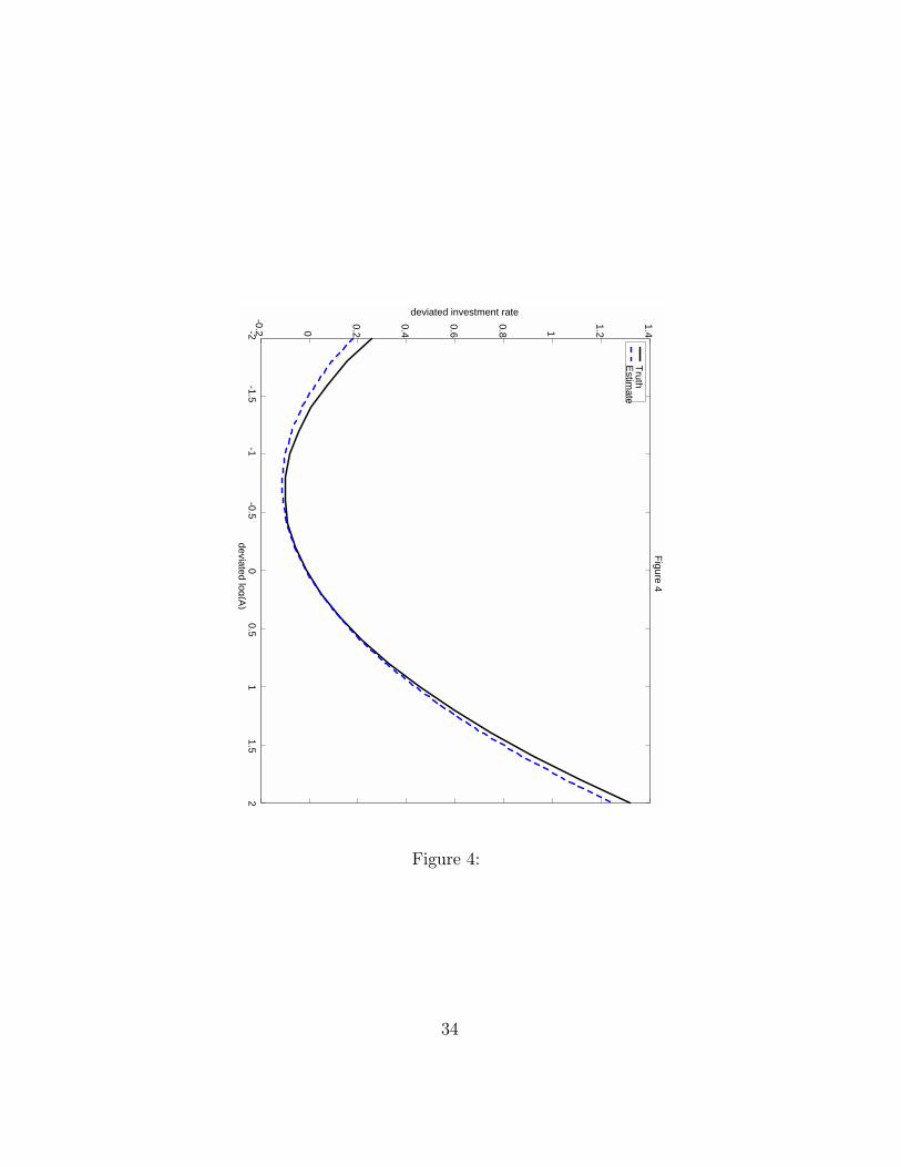
Figure 4 shows the empirical relationship between investment rates andprofitability for the estimated model and Figure 4 shows that relationship us-ing the estimates of the alternative models. Clearly, the full model does cap-ture the nonlinear relationship between investment and fundamentals foundin the data better than any of the restricted models.Using our estimates, we can return to the moments reported in Table 4

which were not explicitly included in the our estimation procedure. Withregard to our motivating themes of inaction and bursts of investment, theestimated model has both features reflecting both the nonconvex adjustmentand the irreversibility of investment. In particular, the estimated model ex-hibits investment spikes (investment rates in excess of 20%) in about 13.7%of the plant year observations compared to the 18% spike rate in the LRD.Further, the investment inaction rate is 52.7% which is substantially higherthan that found in the data. With these estimates, the correlation betweenprofitability and investment is 0.586 while the serial correlation of investmentrates is 0.089. Both of these correlations are much closer to the data than

22

the pure convex model and reflect the fact that the introduction of noncon-vex adjustment costs and irreversibilities reduces both the responsiveness ofinvestment to shocks and its serial correlation.

4.3 Evaluation

Are these results reasonable? Of interest relative to other studies is the rel-atively low estimated value of the convex cost of adjustment parameter, γ.This parameter has received enormous attention in the literature since a re-gression of investment rates on the average value of the firm (Q) will identifythis parameter when the profit function is proportional to K and the costof adjustment function is convex and homogenous of degree one. Using theQ-theoretic approach, estimates of γ range from over 20 (Hayashi [1982]) toas low as 3 (Gilchrist-Himmelberg [1995], unconstrained subsamples, bondrating).Relative to these results, our estimates of γ = .043 for the full model and

γ = .125 in the pure convex model appear extremely low. However, followingCooper-Ejarque [2000], the misspecification of Q-theory based models mayexplain these differences. In particular, when there is curvature in the profitfunction (we estimate θ = .51), the assumptions underlying Q-theory do nothold: i.e. the substitution of average for marginal Q produces a measurementerror. Could this explain the differences in findings about the magnitude ofγ?To study this point, we simulated a panel data set using our estimates.

From this data set and the associated values from the dynamic programmingproblem, we constructed measures of expected discounted average Q.24 Wethen regressed investment rates on these measures of averageQ and used theninferred the value of γ from the regression coefficient on average Q. Whenγ = .043 is used in the simulation, the coefficient on average Q in a regressionof investment rates on a constant and average Q is very precisely estimated at.1427 implying an estimate of γ = 7.01! Thus, the measurement error inducedby replacing marginal with average Q biases the coefficient on average Qdownwards enough to create an inferred value of the convex adjustment costparameter that is well within the range of conventional estimates.25

24Given the one-period time to build, the convex model relates investment to the ex-pected discounted value of the derivative of the value function, as in (7).

25Essentially the substitution of average for marginal Q creates a negative correlationclose to unity between the ”error” and average Q. Of course, this correlation goes to 0 if

23

Further, while others have considered models with nonconvex costs ofadjustment, there are no estimates comparable to our estimate of the fixedcost.26 This estimate implies that the fixed cost of adjustment is about0.04% of average plant level profits. Despite its modest magnitude, thisfixed cost matters for investment decisions. Forcing this parameter to zeroyields nontrivial changes in the reduced form parameter estimates.Put differently, even though this fixed cost may seem small relative to

profits, it can nonetheless be quite influential in terms of decisions if it islarge relative to the gain from adjustment. Formally, define

∆V (A,K) = V act(A,K) + FK − V i(A,K)

where V act is the value of action (regardless of whether it involves buying orselling capital) and V i is the value of inaction. So, ∆V (A,K) measuresthe state contingent gain to action excluding the fixed cost of adjustment(which has been added back). Figure 6 shows ∆V (A,K) and the nonconvexadjustment cost (FK) for a particular value of A as a function of K usingthe estimates of the full model. Note that ∆V (A,K) is less than FK overa substantial range of the capital stock state space. Thus the fixed cost islarge enough to generate inaction over this region.

Our estimates of the degree of irreversibility is within reason, though itis considerably lower (i.e. ps is close to 1) than the estimate provided byRamey and Shapiro [1998] for some plants in the aerospace industry. Asnoted earlier, this level of transactions cost is enough to generate inactivityinstead of sales of capital. Holding the other parameter estimated fixed, ifwe remove the irreversibility by setting ps = 1, the rate of inaction falls toabout 36% and the incidence of investment bursts rises to about 20%. Inthis sense, the presence of even modest transactions costs creates inactionand also dampens the responsiveness of investment to shocks.

the profit function is proportional to K. Cooper-Ejarque develop this point to argue thatthe same measurement error can explain the significance of profit rates in Q regressionsin the absence of capital market imperfections.

26In particular, neither CHP nor CEH estimate adjustment costs directly. Further,while fixed costs of adjustment are present in the Abel and Eberly [1999] model they donot appear to be estimated either.

24

5 Aggregate Implications

The estimation results reported in Table 5 indicate that a model which mixesboth convex and nonconvex adjustment processes can match moments cal-culated from plant level data quite well. An issue for macroeconomists,however, is whether the presence of nonconvexity at the microeconomic level”matters” for aggregate investment. CEH find that introducing the nonlin-earities created by nonconvex adjustment processes can improve the fit ofaggregate investment models. CHP find that the convex adjustment costmodel fits aggregate investment (across their manufacturing plants) reason-ably well on average. However, there are years where the interaction of anupward sloping hazard (investment probability as a function of age) andthe cross sectional distribution of capital vintages does matter for aggregateinvestment.To study the contribution of nonconvex adjustment costs to aggregate

investment (defined by aggregating across the plants in our sample), we com-pare the aggregate implications of our estimated model, termed the best over-all fit model, against two models with convex costs of adjustment. The first,termed the estimated convex model, is the best fit of the pure convex model tothe properties of the micro data as reported in Table 5 (with γ = .125 ). Thesecond, termed the alternative convex model imposes γ = 2,which is closer tothat found in Q-based investment models, described in Gilchrist-Himmelberg[1995] for example. We simulated all three models for 100 periods using thesame draw of aggregate and idiosyncratic shocks. The three simulated timesseries are shown in Figure 7.For this exercise, we treat the aggregate time series created by the best

overall fit model as ”truth” and consider how well the alternative convexadjustment costs models match this time series. It is apparent that the al-ternative convex model does very poorly in terms of its aggregate dynamics.Aggregate investment from this specification is much smoother than thatimplied by the best overall fit model. Note, however, that the aggregate in-vestment implied by the estimated convex model does a reasonably good jobof matching the aggregate investment behavior of the best overall fit model.For this latter comparison, there are differences at ”turning points” whenthe aggregate shock changes from one state to another. In particular, whenthe aggregate shock switches from below to above its mean, the resultingburst of investment is much higher for the best overall fit model than for theestimated convex model.

25

Using these three series, we computed a pseudo R2 measure defined asthe fraction of the fluctuations in the aggregate investment rate that areexplained by the alternative convex models.27 For the series shown in Figure7, this measure of goodness of fit for the alternative convex model is 0.22 whileit is 0.93 for the estimated convex model. These findings along with Figure 7suggest that the alternative convex model, parameterized at ”conventional”levels, yields aggregate dynamics that are far from those associated withthe best overall fit model. However, the estimated convex model (which hasquite weak convexity) yields aggregate patterns that are not too far fromthose implied by the best fit model.28

In our simulated environment, we can explore the factors that yield in-creases or decreases the fraction that can be accounted for by the convexmodel. If we double the variance of aggregate shocks for example thispseudo R2 measure for the best fit convex model drops to 91.7%.29 Thissensitivity to the magnitude of the aggregate shocks is intuitive as largeraggregate shocks push the distribution of plants into different regions of thenonlinear relationship between investment and fundamentals that are a keyfeature of models with nonconvexities. This finding is important in practicebecause it suggests that the micro nonconvexities that we estimate as beingimportant in the micro data are likely to be most important empirically foraggregate investment at times of especially large shocks.It is also of interest to ask the question how well does the estimated

convex model fit the overall distribution of investment rates. One way ofanswering this question is to compute the pseudo R2 using the simulatedplant level data for the pure and mixed cases. Computing the pseudo R2

measure in this manner for the estimated convex model yields 0.79. Notsurprisingly, smoothing by aggregation implies that the convex model doesrelatively better in matching aggregate relative to plant level data.This analysis of the aggregate implications is potentially incomplete in

that we do not explicitly consider general equilibrium considerations. As

27Letting ε be the difference between aggregate investment from the estimated model(est) and the convex model, we defined our goodness of fit measure as 1-var(ε)/(var(est)).

28This finding that approximately ninety percent of the aggregate fluctuations in invest-ment can be accounted for with convex cost elements alone is roughly consistent with thefindings in CEH and CHP. For example, in CEH, a regression of aggregate investment onthe first moment of the gap between desired and actual capital yielded a R2 of roughly.65 while adding higher moments raised the pseudo R2 measure to 0.80.

29That is, the aggregate shocks take the values {.8,1.2} instead of {.9,1.1}.

26

emphasized by Veracierto [1998], Caballero [1999] and Thomas [2000], it islikely that there is further smoothing by aggregation due to the congestioneffects that are potentially present in the capital goods supply industry. Ourfocus here is more of a pure aggregation exercise considering the aggregateimplications of the alternative mixed and pure specifications of structuralmodels given the distributions of aggregate and idiosyncratic shocks.

6 Conclusions

The goal of this paper is to analyze capital dynamics through competingmodels of the investment process: what is the nature of the capital adjust-ment process? The methodology is to take a model of the capital adjustmentprocess with a rich specification of adjustment costs and solve the dynamicoptimization problem at the plant level. Using the resulting policy functionsto create a simulated data set, the procedure of indirect inference is used toestimate the structural parameters.Our empirical results point to the mixing of models of the adjustment

process. The LRD indicates that plants exhibit periods of inactivity as wellas large investment bursts. Further, the relationship between investmentrates and measures of profitability at the plant level is highly nonlinear. Amodel which incorporates both convex and nonconvex aspects of adjustment,including irreversibility, fits these observations best.In terms of further consideration of these issues, we plan to continue this

line of research by introducing costs of employment adjustment. This ispartially motivated by the ongoing literature on adjustment costs for laboras well as the fact that the model without labor adjustment costs implieslabor movements that are not consistent with observation.Further, it would be insightful to utilize this model to study the effects

of investment tax subsidies. Here those subsidies enter quite easily throughpolicy induced variations in the cost of capital.

27

References

[1] Abel, A. and J. Eberly, ”A Unified Model of Investment under Uncer-tainty,” American Economic Review, 84 (1994), 1369-84.

[2] Abel, A. and J. Eberly, ”Optimal Investment with Costly Reversibility,”Review of Economic Studies,”63 (1996), 581-93.

[3] Abel, A. and J. Eberly, ”The Mix and Scale of Factors with Irreversibil-ity and Fixed Costs of Investment,” NBERWorking Paper #6148, 1997.

[4] Abel, A. and J. Eberly, ”Investment and q with Fixed Costs: An Em-pirical Analysis,” mimeo, April 1999.

[5] Caballero, R., ”Aggregate Investment,” in Handbook of Macroeconomics,(edited by J. Taylor and M. Woodford), Amsterdam: North Holland,1999.

[6] Caballero, R., E. Engel and J. Haltiwanger, ”Plant-level Adjustmentand Aggregate Investment Dynamics,” Brookings Papers on EconomicActivity, 2 (1995), 1-39.

[7] Caballero, R., E. Engel and J. Haltiwanger, ”Aggregate EmploymentDynamics: Building from Microeconomic Evidence,” American Eco-nomic Review 87 (1997), 115-37.

[8] Cooper, R. and J. Ejarque, ”Exhuming Q:Market Power vs.Capital Mar-ket Imperfections” mimeo, Boston University, August 2000.

[9] Cooper, R. and J. Haltiwanger, ”The Aggregate Implications of MachineReplacement: Theory and Evidence,” American Economic Review, 83(1993), 360-82.

[10] Cooper, R., J. Haltiwanger and L. Power, ”Machine Replacement andthe Business Cycle: Lumps and Bumps,” American Economic Review,89 (1999), 921-946.

[11] Doms, M. and T. Dunne,”Capital Adjustment Patterns in Manufactur-ing Plants,” Center for Economic Studies, U.S. Bureau of the Census,1993.

28

[12] Gilchrist, S. and C. Himmelberg, ”The Role of Cash Flow in Reduced-Form Investment Equations,” Journal of Monetary Economics, 1995.

[13] Gilchrist, S. and C. Himmelberg, ”Investment, Fundamentals and Fi-nance,” The NBER Macroeconomics Annual, 1998.

[14] Gomes, J. ”Financing Investment,” mimeo, Wharton School, Universityof Pennsylvania, January 1998.

[15] Goolsbee, A. ”The Business Cycle, Financial Performance and the Re-tirement of Capital Goods,” NBER Working Paper #6392, February1998.

[16] Goolsbee, A. and D. Gross, ”Estimating Adjustment Costs with Dataon Heterogeneous Capital Goods,” NBER Working Paper #6342, De-cember 1997.

[17] Hayashi, F. ”Tobin’s Marginal and Average q: A Neoclassical Interpre-tation,” Econometrica 50 (1982), 213-24

[18] Hamermesh, D. ”Labor Demand and the Structure of AdjustmentCosts,” American Economic Review, 79 (1989), 674-89.

[19] Hamermesh, D. and G. Pfann, ”Adjustment Costs in Factor Demand,”Journal of Economic Literature, 34 (1996), 1264-92.

[20] Holt, C., F. Modigliani, J. Muth, H. Simon, Planning Production, Inven-tories, and Work Force, Englewood Cliffs, N.J.: Prentice-Hall, 1960.

[21] Huggett, M and S. Ospina, ”Does Productivity Fall After the Adoptionof New Technology?”mimeo, September 1998.

[22] Nilsen, O. and F. Schiantarelli, ”Zeroes and Lumps in Investment: Em-pirical Evidence on Irreversibilities and nonconvexities,” mimeo, BostonCollege, March 1998.

[23] Peck, S. ”Alternative Investment Models for firms in the Electric Util-ities Industry,” Bell Journal of Economics and Management Science, 5(1974), 420-457.

[24] Ramey, V. and M. Shapiro, ”Displaced Capital,” mimeo, University ofCalifornia, San Diego, March 1998.

29

[25] Rothschild, M. ”On the Cost of Adjustment,” Quarterly Journal of Eco-nomics 85 (1971), 605-22.

[26] Smith, A. ”Estimating Nonlinear Time-Series Models Using SimulatedVector Autoregressions,” Journal of Applied Econometrics, 8 (1993),S63-S84.

[27] Thomas, J. ”Is Lumpy Investment Relevant for the Business Cy-cle?,mimeo, Carnegie-Mellon University, August 2000. ”

[28] Veracierto, M. ”Plant Level Irreversible Investment and EquilibriumBusiness Cycles,” Working Paper 98-1, Federal Reserve Bank ofChicago, February 1998.

30

PER

CEN

T 0123456789

10

11

Inve

stm

en

tR

ate

- 0 . 2 0

- 0 . 1 8

- 0 . 1 6

- 0 . 1 4

- 0 . 1 2

- 0 . 1 0

- 0 . 0 8

- 0 . 0 6

- 0 . 0 4

- 0 . 0 2

- 0 . 0 0

0 . 0 20 . 0 4

0 . 0 60 . 0 8

0 . 1 00 . 1 2

0 . 1 40 . 1 6

0 . 1 80 . 2 0

0 . 2 20 . 2 4

0 . 2 60 . 2 8

0 . 3 00 . 3 2

0 . 3 40 . 3 6

0 . 3 80 . 4 0

0 . 4 20 . 4 4

0 . 4 60 . 4 8

0 . 5 00 . 5 2

Figure 1:

31

-2 -1.5 -1 -0.5 0 0.5 1 1.5 2-0.2

0

0.2

0.4

0.6

0.8

1

1.2

1.4Figure 2

devi

ated

inve

stm

ent r

ate

deviated log(A)

-1 -0.8 -0.6 -0.4 -0.2 0 0.2 0.4 0.6 0.8 10

0.02

0.04

0.06

0.08

0.1

0.12

0.14

0.16

fract

ion

deviated log(A)

Figure 2:

32

-2-1.5

-1-0.5

00.5

11.5

2-0.5 0

0.5 1

1.5 2

2.5 3Figure 3

deviated investment rate

deviated log(A)

Convex

Nonconvex (F)

Nonconvex (qs)

No adj. costs

Figure 3:

33

-2-1.5

-1-0.5

00.5

11.5

2-0.2 0

0.2

0.4

0.6

0.8 1

1.2

1.4Figure 4

deviated investment rate

deviated log(A)

Truth Estim

ate

Figure 4:

34

-2-1.5

-1-0.5

00.5

11.5

2-0.2 0

0.2

0.4

0.6

0.8 1

1.2

1.4

1.6

1.8Figure 5

deviated investment rate

deviated log(A)

Truth C

onvex N

onconvex (F) N

onconvex (qs)

Figure 5:

35

2040

6080

100120

140160

180200

-200 0

200

400

600

800

1000

1200

1400

1600Figure 6

capital states

diff. of valuesfixed cost

Figure 6:

36

010

2030

4050

6070

8090

100-0.05 0

0.05

0.1

0.15

0.2

0.25

0.3Figure 7

aggregate investment rate

simulated tim

e series

Best Overall Fit M

odelEstim

ated Convex M

odelAlt. C

onvex Model

Figure 7:

37