A Note on Indeterminacy and InvestmentAdjustment Costs in an Endogenously Growing

Small Open Economy∗

Chi-Ting Chin†

Ming Chuan UniversityJang-Ting Guo‡

University of California, Riverside

Ching-Chong Lai§

Academia SinicaNational Chengchi University

August 26, 2010

Abstract

This note analytically examines the interrelations between macroeconomic (in)stabilityand investment adjustment costs in a one-sector endogenously growing small-open-economyrepresentative agent model. We show that under costly capital accumulation, the economyexhibits indeterminacy and sunspots if and only if the equilibrium wage-hours locus slopesupwards and is steeper than the household’s labor supply curve. By contrast, the econ-omy without adjustment costs for capital investment always displays saddle-path stabilityand equilibrium uniqueness, regardless of the degree of increasing returns in aggregateproduction.

Keywords: Indeterminacy; Investment Adjustment Costs; Endogenous Growth; SmallOpen Economy.

JEL Classification: E22; E32; F41; O41.

∗We would like to thank William Barnett (the Editor), an Associate Editor, two anonymous referees, Juin-Jen Chang, Sharon Harrison, Richard Suen, Stephen Turnovsky, and seminar participants at National CentralUniversity (Taiwan) and National Tsing Hua University (Taiwan) for helpful discussions and comments. Partof this research was conducted while Guo was a visiting research fellow of economics at Academia Sinica, whosehospitality is greatly appreciated. Of course, all remaining errors are our own.†Department of Risk Management and Insurance, Ming Chuan University, Taipei 111, Taiwan, 886-2-2882-

4564, ext. 2613, Fax: 886-2-2880-9755, E-mail: debbyjin@zeta.mcu.edu.tw.‡Corresponding Author. Department of Economics, 4123 Sproul Hall, University of California, Riverside,

CA, 92521, USA, 1-951-827-1588, Fax: 1-951-827-5685, E-mail: guojt@ucr.edu.§Institute of Economics, Academia Sinica, 128 Yen-Chiu-Yuan Road, Section 2, Taipei 115, Taiwan, 886-

2-2782-2791, ext. 645, Fax: 886-2-2785-3946, E-mail: cclai@econ.sinica.edu.tw. Department of Economics,National Chengchi University, Taipei 116, Taiwan.

1 Introduction

It is now well known that dynamic general equilibrium macroeconomic models may possess

an indeterminate steady state or balanced growth path that can be exploited to generate

business cycle fluctuations driven by agents’ self-fulfilling beliefs. In particular, Benhabib

and Farmer (1994) show that one-sector representative agent models for a closed economy

exhibit indeterminacy and sunspots under suffi ciently strong increasing returns in aggregate

production.1 Subsequently, Kim (2003) finds that (both analytically and quantitatively) in the

no-sustained-growth version of Benhabib and Farmer’s model, the minimum level of returns-

to-scale needed for equilibrium indeterminacy is ceteris paribus a monotonically increasing

function of the size of investment adjustment costs.2 It is straightforward to show that the

same result also holds in the endogenous-growth specification of the Benhabib-Farmer closed

economy. Intuitively, investment adjustment costs are observationally equivalent to a state-

contingent tax that “leans against the wind” of intertemporal capital accumulation. As a

result, when the representative agent becomes optimistic about the economy’s future and

decides to invest more, the presence of investment adjustment costs will raise the required

degree of aggregate increasing returns to fulfill the household’s initial optimism.3

In this note, we build upon Kim’s (2003) analyses and explore the theoretical interrelations

between equilibrium indeterminacy and investment adjustment costs in the endogenous-growth

version of Benhabib and Farmer’s (1994) one-sector representative agent model for a small open

economy. This specification provides us a useful analytical benchmark as well as facilitates

comparison with recent studies (e.g. Lahiri (2001), Weder (2001), and Meng and Velasco

(2003, 2004), among others) that examine the condition(s) for indeterminacy and sunspots

in closed-economy versus small-open-economy macroeconomic models with two sectors and

no adjustment costs. Under the assumption of perfect international capital markets, the

domestic households are able to lend to and borrow from abroad freely.4 To guarantee positive

1See Benhabib and Farmer (1999) for an excellent survey on this strand of the indeterminacy literature.2Wen (1998) numerically verifies this positive relationship in a calibrated one-sector real business cycle model

where capital adjustment costs are postulated as a quadratic function of the difference in gross investmentsbetween two consecutive time periods.

3A corollary of this finding is that adjustment costs for capital investment can be used to eliminate equilib-rium multiplicity and select a locally unique equilibrium in the Benhabib-Farmer economy (Guo and Lansing,2002, pp. 655 − 657). The same result is obtained in different one-sector macroeconomic models for a closedeconomy (Georges, 1995) or in a two-sector representative agent model with sector-specific externalities for asmall open economy (Herrendorf and Valentinyi, 2003).

4Aguiar-Conraria and Wen (2008) and Chen and Zhang (2009) examine the interrelations between equilib-rium indeterminacy and production externalities in one-sector no-sustained-growth models for an open economywithout access to a perfect world capital market and investment adjustment costs.

1

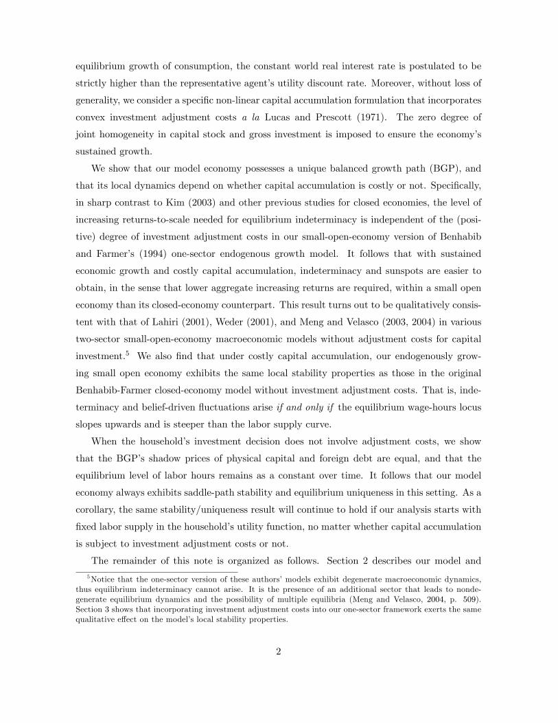
equilibrium growth of consumption, the constant world real interest rate is postulated to be

strictly higher than the representative agent’s utility discount rate. Moreover, without loss of

generality, we consider a specific non-linear capital accumulation formulation that incorporates

convex investment adjustment costs a la Lucas and Prescott (1971). The zero degree of

joint homogeneity in capital stock and gross investment is imposed to ensure the economy’s

sustained growth.

We show that our model economy possesses a unique balanced growth path (BGP), and

that its local dynamics depend on whether capital accumulation is costly or not. Specifically,

in sharp contrast to Kim (2003) and other previous studies for closed economies, the level of

increasing returns-to-scale needed for equilibrium indeterminacy is independent of the (posi-

tive) degree of investment adjustment costs in our small-open-economy version of Benhabib

and Farmer’s (1994) one-sector endogenous growth model. It follows that with sustained

economic growth and costly capital accumulation, indeterminacy and sunspots are easier to

obtain, in the sense that lower aggregate increasing returns are required, within a small open

economy than its closed-economy counterpart. This result turns out to be qualitatively consis-

tent with that of Lahiri (2001), Weder (2001), and Meng and Velasco (2003, 2004) in various

two-sector small-open-economy macroeconomic models without adjustment costs for capital

investment.5 We also find that under costly capital accumulation, our endogenously grow-

ing small open economy exhibits the same local stability properties as those in the original

Benhabib-Farmer closed-economy model without investment adjustment costs. That is, inde-

terminacy and belief-driven fluctuations arise if and only if the equilibrium wage-hours locus

slopes upwards and is steeper than the labor supply curve.

When the household’s investment decision does not involve adjustment costs, we show

that the BGP’s shadow prices of physical capital and foreign debt are equal, and that the

equilibrium level of labor hours remains as a constant over time. It follows that our model

economy always exhibits saddle-path stability and equilibrium uniqueness in this setting. As a

corollary, the same stability/uniqueness result will continue to hold if our analysis starts with

fixed labor supply in the household’s utility function, no matter whether capital accumulation

is subject to investment adjustment costs or not.

The remainder of this note is organized as follows. Section 2 describes our model and

5Notice that the one-sector version of these authors’models exhibit degenerate macroeconomic dynamics,thus equilibrium indeterminacy cannot arise. It is the presence of an additional sector that leads to nonde-generate equilibrium dynamics and the possibility of multiple equilibria (Meng and Velasco, 2004, p. 509).Section 3 shows that incorporating investment adjustment costs into our one-sector framework exerts the samequalitative effect on the model’s local stability properties.

2

analyzes the equilibrium conditions. Section 3 examines local dynamics of the economy’s

balanced growth path with or without investment adjustment costs. Section 4 concludes.

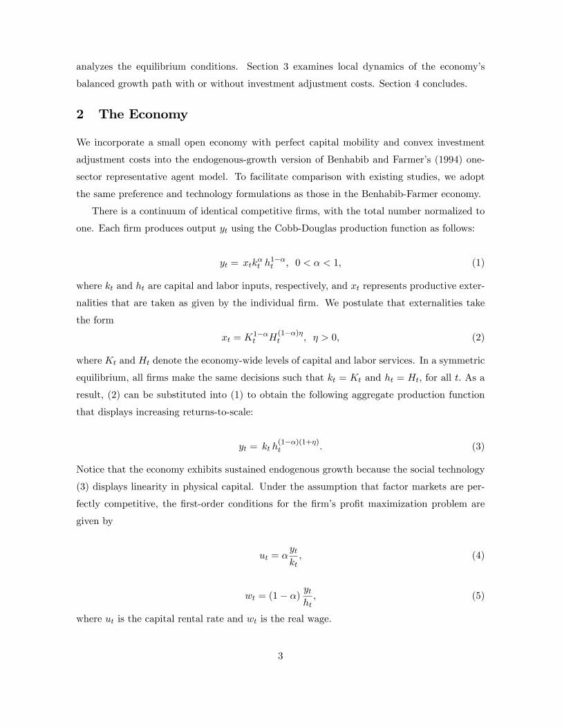
2 The Economy

We incorporate a small open economy with perfect capital mobility and convex investment

adjustment costs into the endogenous-growth version of Benhabib and Farmer’s (1994) one-

sector representative agent model. To facilitate comparison with existing studies, we adopt

the same preference and technology formulations as those in the Benhabib-Farmer economy.

There is a continuum of identical competitive firms, with the total number normalized to

one. Each firm produces output yt using the Cobb-Douglas production function as follows:

yt = xtkαt h

1−αt , 0 < α < 1, (1)

where kt and ht are capital and labor inputs, respectively, and xt represents productive exter-

nalities that are taken as given by the individual firm. We postulate that externalities take

the form

xt = K1−αt H

(1−α)ηt , η > 0, (2)

where Kt and Ht denote the economy-wide levels of capital and labor services. In a symmetric

equilibrium, all firms make the same decisions such that kt = Kt and ht = Ht, for all t. As a

result, (2) can be substituted into (1) to obtain the following aggregate production function

that displays increasing returns-to-scale:

yt = kt h(1−α)(1+η)t . (3)

Notice that the economy exhibits sustained endogenous growth because the social technology

(3) displays linearity in physical capital. Under the assumption that factor markets are per-

fectly competitive, the first-order conditions for the firm’s profit maximization problem are

given by

ut = αytkt, (4)

wt = (1− α)ytht, (5)

where ut is the capital rental rate and wt is the real wage.

3

The economy is also populated by a unit measure of identical infinitely-lived households,

each has one unit of time endowment and maximizes a discounted stream of utilities over its

lifetime

∫ ∞0

{log ct −A

h1+γt

1 + γ

}e−ρtdt, A > 0, (6)

where ct is the individual household’s consumption, γ ≥ 0 denotes the inverse of the intertem-

poral elasticity of substitution in labor supply, and ρ > 0 is the discount rate. The budget

constraint faced by the representative household is given by

ct + it + bt = utkt + wtht + rbt, k0 > 0 and b0 are given, (7)

where it is gross investment, and r > 0 is the exogenously-given constant world real interest rate

on risk-free foreign bonds bt. Under the assumption of perfect international capital markets,

the domestic household is able to lend to and borrow from abroad freely.

As in Kim (2003, p. 400), the law of motion for capital stock is specified as

ktkt

= Ψ

(itkt

)=

δ

[(itδkt

)1−θ−1

]1−θ , θ ≥ 0, θ 6= 1

δ log(itδkt

), θ = 1,

(8)

where δ ∈ (0, 1) is the capital depreciation rate. When θ > 0, the resulting non-linear formu-

lation is an increasing and concave function of the investment-to-capital ratio itkt. This feature

can be viewed as reflecting convex adjustment costs a la Lucas and Prescott (1971); and the

elasticity parameter θ(≡ − δΨ

′′(δ)

Ψ′(δ)

)represents the degree (or size) of investment adjustment

costs.6 When θ = 0, (8) becomes the standard linear capital accumulation equation with-

out adjustment costs. Finally, the zero degree of joint homogeneity in it and kt is needed to

maintain the economy’s balanced growth in output, consumption and investment.7

The first-order conditions for the representative household with respect to the indicated

6Notice that when θ = 1, (8) corresponds to the loglinear law of motion for capital stock in discretetime whereby kt+1 = k1−δt

(itδ

)δ, 0 < δ < 1. In this case, Guo and Lansing (2003) find that Benhabib

and Farmer’s (1994) closed-economy model always exhibits saddle-path stability and equilibrium uniqueness.However, section 3.1 shows that this result does not hold in our endogenously growing small-open-economymodel.

7All the (in)determinacy results reported below remain unaffected under Hayashi’s (1982) adjustment-costformulation. In particular, the Appendix examines the following expenditure function for total investment thatincludes capital installation costs and is consistent with sustained economic growth: it(1+ φ

2itkt), where φ > 0.

4

variables and the associated transversality conditions (TVC) are

ct :1

ct= λat, (9)

ht : Ahγt = λatwt, (10)

it : λkt

(itδkt

)−θ= λat, (11)

kt : λkt = ρλkt −δλkt

[θ(itδkt

)1−θ− 1

]1− θ − λatut, (12)

bt : λat = (ρ− r)λat, (13)

TVC1 : limt→∞

e−ρtλatbt = 0, (14)

TVC2 : limt→∞

e−ρtλktkt = 0, (15)

where λat and λkt are the shadow prices of asset (foreign bonds) and physical capital, re-

spectively. Equation (9) states that the marginal benefit of consumption equals its marginal

cost, which is the marginal utility of having an additional unit of internationally traded bonds.

Moreover, equation (10) equates the slope of the representative household’s indifference curve

to the real wage, and equations (11) and (12) together govern the evolution of capital stock

over time. Finally, equation (13) states that the marginal utility values of foreign debt holdings

are equal to their respective marginal costs.

Combining equations (9) and (13) yields the following standard Keynes-Ramsey rule:

ctct

= r − ρ. (16)

To guarantee positive equilibrium growth of consumption, we assume that the world interest

rate is strictly higher than the household’s utility discount rate, i.e. r > ρ.

3 Analysis of Dynamics

We focus on the economy’s balanced growth path (BGP) along which labor hours are sta-

tionary, and output, consumption, physical capital and foreign bonds all exhibit a common,

positive constant growth rate given by r− ρ. To facilitate the analysis of perfect-foresight dy-namics under sustained economic growth, we make the following transformation of variables:

qt ≡ λkt/λat, zt ≡ ct/kt and xt ≡ bt/ct. Notice that qt corresponds to “Tobin’s q”which

defines the marginal utility value of physical capital measured in terms of the shadow price of

foreign bonds.

5

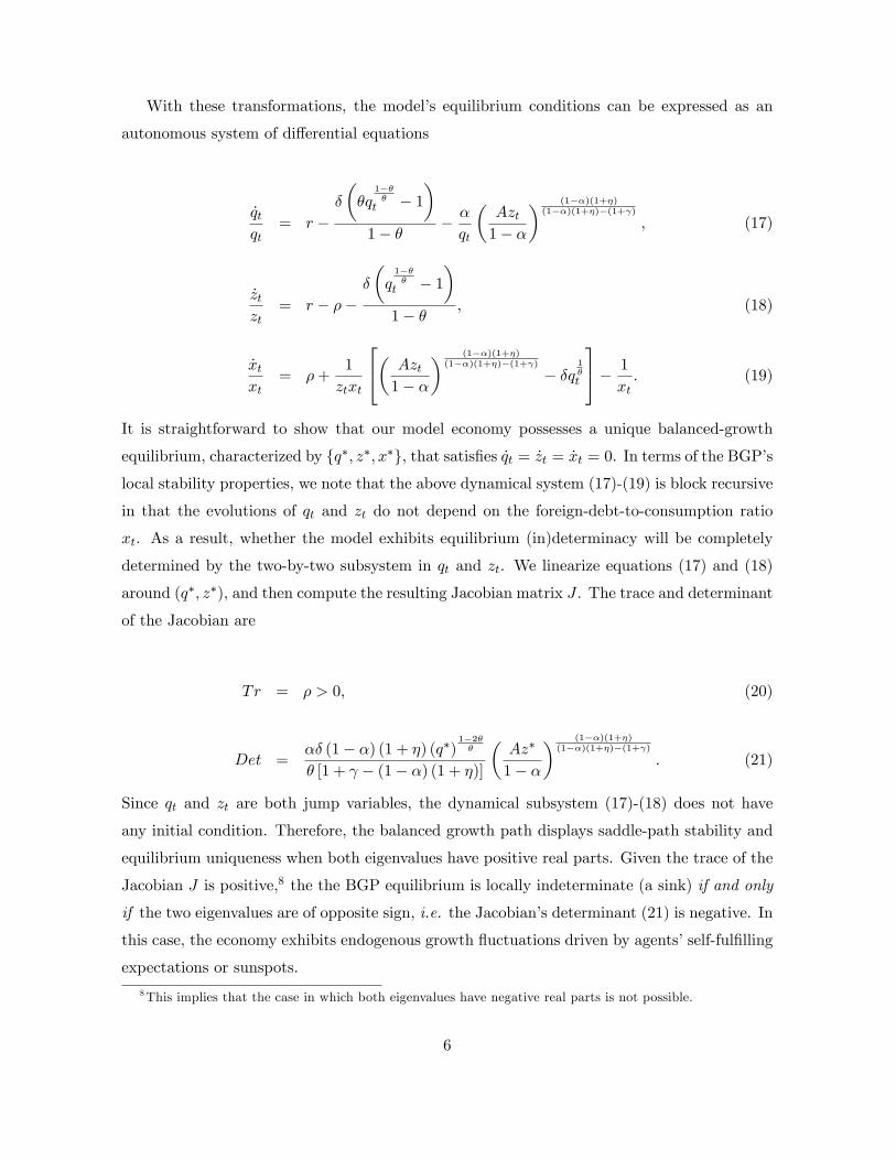
With these transformations, the model’s equilibrium conditions can be expressed as an

autonomous system of differential equations

qtqt

= r −δ

(θq

1−θθ

t − 1

)1− θ − α

qt

(Azt

1− α

) (1−α)(1+η)(1−α)(1+η)−(1+γ)

, (17)

ztzt

= r − ρ−δ

(q1−θθ

t − 1

)1− θ , (18)

xtxt

= ρ+1

ztxt

( Azt1− α

) (1−α)(1+η)(1−α)(1+η)−(1+γ)

− δq1θt

− 1

xt. (19)

It is straightforward to show that our model economy possesses a unique balanced-growth

equilibrium, characterized by {q∗, z∗, x∗}, that satisfies qt = zt = xt = 0. In terms of the BGP’s

local stability properties, we note that the above dynamical system (17)-(19) is block recursive

in that the evolutions of qt and zt do not depend on the foreign-debt-to-consumption ratio

xt. As a result, whether the model exhibits equilibrium (in)determinacy will be completely

determined by the two-by-two subsystem in qt and zt. We linearize equations (17) and (18)

around (q∗, z∗), and then compute the resulting Jacobian matrix J . The trace and determinant

of the Jacobian are

Tr = ρ > 0, (20)

Det =αδ (1− α) (1 + η) (q∗)

1−2θθ

θ [1 + γ − (1− α) (1 + η)]

(Az∗

1− α

) (1−α)(1+η)(1−α)(1+η)−(1+γ)

. (21)

Since qt and zt are both jump variables, the dynamical subsystem (17)-(18) does not have

any initial condition. Therefore, the balanced growth path displays saddle-path stability and

equilibrium uniqueness when both eigenvalues have positive real parts. Given the trace of the

Jacobian J is positive,8 the the BGP equilibrium is locally indeterminate (a sink) if and only

if the two eigenvalues are of opposite sign, i.e. the Jacobian’s determinant (21) is negative. In

this case, the economy exhibits endogenous growth fluctuations driven by agents’self-fulfilling

expectations or sunspots.

8This implies that the case in which both eigenvalues have negative real parts is not possible.

6

3.1 When θ > 0

In this specification, the non-linear capital accumulation equation (8) exhibits convex invest-

ment adjustment costs. It is straightforward to show that the BGP equilibrium is characterized

by a pair of positive real numbers (q∗, z∗) given by9

q∗ =

[

(1−θ)(r−ρ)+δδ

] θ1−θ

, θ ≥ 0, θ 6= 1

exp[ r−ρ

δ

], θ = 1,

(22)

z∗ =

(

1−αA

) [ (1−θ)r+δ+θρα

] (1−α)(1+η)−(1+γ)(1−α)(1+η)

[(1−θ)(r−ρ)+δ

δ

] θ[(1−α)(1+η)−(1+γ)](1−θ)(1−α)(1+η)

, θ ≥ 0, θ 6= 1(1−αA

){(ρ+δα

)exp

[ r−ρδ

]} (1−α)(1+η)−(1+γ)(1−α)(1+η)

, θ = 1.

(23)

Since q∗, z∗, A, η, θ > 0, 0 < α, δ < 1, and γ ≥ 0, the Jacobian’s determinant (21) is negative

if and only if

(1− α) (1 + η)− 1 > γ, (24)

which is also the necessary and suffi cient condition for our model economy to display equilib-

rium indeterminacy and belief-driven aggregate fluctuations.

To understand the above indeterminacy condition, we first substitute (9) into (10) and

find that agents’equilibrium decision on hours worked is governed by

Acthγt = wt. (25)

Next, plugging the aggregate production function (3) into the logarithmic version of firms’

labor demand condition (5) shows that the slope of the equilibrium wage-hours locus is equal

to (1− α) (1 + η)− 1. In addition, taking logarithms on both sides of (25) indicates that the

slope of the household’s labor supply curve is γ (≥ 0), and its position or intercept is affected

by the level of consumption. It follows that the condition that is needed to generate inde-

terminacy and sunspots, as in (24), states that the equilibrium wage-hours locus is positively

sloped and steeper than the labor supply curve. Interestingly, (24) turns out to be identical to

9The remaining endogenous variables on the economy’s balanced growth path can then be derived ac-cordingly. In particular, the BGP’s investment-to-capital ratio and hours worked are

(ik

)∗= δ (q∗)

1θ and

h∗ =(Az∗

1−α

) 1(1−α)(1+η)−(1+γ)

, respectively. Moreover, the requirement of a positive q∗ or(ik

)∗yields the follow-

ing upper bound on the size of investment adjustment costs: θ < 1 + δr−ρ .

7

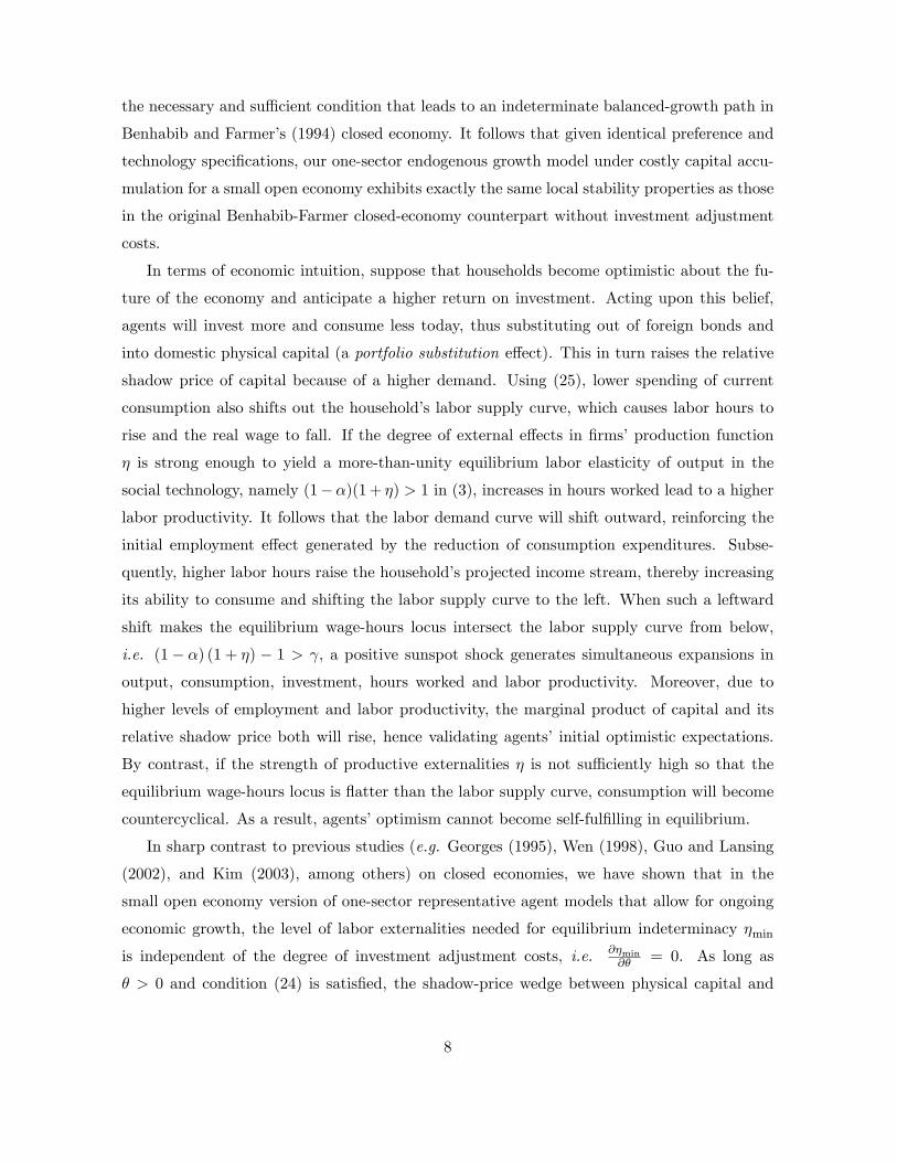
the necessary and suffi cient condition that leads to an indeterminate balanced-growth path in

Benhabib and Farmer’s (1994) closed economy. It follows that given identical preference and

technology specifications, our one-sector endogenous growth model under costly capital accu-

mulation for a small open economy exhibits exactly the same local stability properties as those

in the original Benhabib-Farmer closed-economy counterpart without investment adjustment

costs.

In terms of economic intuition, suppose that households become optimistic about the fu-

ture of the economy and anticipate a higher return on investment. Acting upon this belief,

agents will invest more and consume less today, thus substituting out of foreign bonds and

into domestic physical capital (a portfolio substitution effect). This in turn raises the relative

shadow price of capital because of a higher demand. Using (25), lower spending of current

consumption also shifts out the household’s labor supply curve, which causes labor hours to

rise and the real wage to fall. If the degree of external effects in firms’production function

η is strong enough to yield a more-than-unity equilibrium labor elasticity of output in the

social technology, namely (1−α)(1 + η) > 1 in (3), increases in hours worked lead to a higher

labor productivity. It follows that the labor demand curve will shift outward, reinforcing the

initial employment effect generated by the reduction of consumption expenditures. Subse-

quently, higher labor hours raise the household’s projected income stream, thereby increasing

its ability to consume and shifting the labor supply curve to the left. When such a leftward

shift makes the equilibrium wage-hours locus intersect the labor supply curve from below,

i.e. (1− α) (1 + η) − 1 > γ, a positive sunspot shock generates simultaneous expansions in

output, consumption, investment, hours worked and labor productivity. Moreover, due to

higher levels of employment and labor productivity, the marginal product of capital and its

relative shadow price both will rise, hence validating agents’ initial optimistic expectations.

By contrast, if the strength of productive externalities η is not suffi ciently high so that the

equilibrium wage-hours locus is flatter than the labor supply curve, consumption will become

countercyclical. As a result, agents’optimism cannot become self-fulfilling in equilibrium.

In sharp contrast to previous studies (e.g. Georges (1995), Wen (1998), Guo and Lansing

(2002), and Kim (2003), among others) on closed economies, we have shown that in the

small open economy version of one-sector representative agent models that allow for ongoing

economic growth, the level of labor externalities needed for equilibrium indeterminacy ηmin

is independent of the degree of investment adjustment costs, i.e. ∂ηmin∂θ = 0. As long as

θ > 0 and condition (24) is satisfied, the shadow-price wedge between physical capital and

8

foreign bonds will produce the above-mentioned effects of portfolio substitution and labor

adjustments in response to agents’optimistic expectations. On the contrary, such portfolio-

substitution opportunities do not exist within a closed economy because the only asset available

to households is domestic capital stock. Consequently, ηmin is monotonically increasing with

respect to the size of adjustment costs for capital investment in order to fulfill households’

optimism(∂ηmin∂θ > 0

).

This “independence”finding also implies that under sustained economic growth and costly

capital accumulation, indeterminacy and sunspots are more likely to arise, in the sense that

lower increasing returns are required, within a small-open-economy than a closed-economy

setting.10 Notice that Lahiri (2001), Weder (2001), and Meng and Velasco (2003, 2004) obtain

the same result in various two-sector small-open-economy macroeconomic models without

investment adjustment costs. Due to perfect capital mobility, the models that these authors

examine behave like a closed economy with linear preferences in consumption. It follows that

there are no utility costs associated with constructing alternative equilibrium paths when

agents become optimistic. In comparison with the corresponding closed economy, this feature

in turn enlarges the range of parameter values under which indeterminacy and sunspots may

occur in a small-open-economy formulation.

Finally, in the no-sustained-growth version of our one-sector small-open-economy model

with investment adjustment costs, we find that international lending and borrowing lead to

complete consumption smoothing, i.e. the level of equilibrium consumption ct is a fixed con-

stant over time (see equation 16 under the knife-edge condition r = ρ, and Turnovsky (2002)

for more general discussions). Therefore, in response to agent’s optimism about the economy’s

future, the outward shift of the household’s labor supply curve described earlier will not take

place. On the other hand, the portfolio substitution (from foreign bonds to domestic phys-

ical capital) effect alone is not suffi ciently strong to raise the rate of return on investment

because the firm’s production technology now displays diminishing marginal product of cap-

ital. It follows that the steady state is a saddle point within this configuration. The same

intuition for saddle-path stability can be applied to our model with exogenous growth, based

on labor-augmenting technological progress st, in that the detrended consumption ct/st will

10For example, under Kim’s (2003, p. 399) benchmark parameterization with α = 0.3, γ = 0, ρ = 0.05,δ = 0.1, and θ = 0.05, we find that ηmin = 0.74 for a closed-economy model, whereas ηmin = 0.43 in itssmall-open-economy counterpart. Although the latter value of ηmin is smaller, the resulting aggregate returns-to-scale is nevertheless empirically implausible. Therefore, the preceding calibrated example should be viewedmore from a methodological perspective as it quantitatively illustrates the stability effects of costly capitalaccumulation in a one-sector endogenously growing closed-economy versus small-open-economy model.

9

remain time invariant along the economy’s equilibrium growth path.11 Overall, the above

analysis illustrates that endogenous growth is necessary for the possibility of indeterminacy

and sunspots in a small open economy.

3.2 When θ = 0

In this specification, the capital accumulation equation (8) is linear and does not exhibit

investment adjustment costs. Substituting θ = 0 into (11) shows that the relative price (in

utility terms) of physical capital to internationally traded bonds qt ≡ λkt/λat = 1 for all t. As

a result, the dynamical subsystem (17)-(18) now becomes degenerate. Resolving our model

with θ = 0 and qt = 1 leads to the following single differential equation in xt ≡ bt/ct that

describes the equilibrium dynamics:

xtxt

= ρ+1

xt

A [(1− α) r + αρ]

α (1− α)

(r + δ

α

) (1+γ)−(1−α)(1+η)(1−α)(1+η)

− 1

, (26)

which has a unique interior solution x∗ that satisfies xt = 0 along the balanced-growth equilib-

rium path. We then linearize (26) around the BGP and find that its local stability properties

are governed by ρ > 0. Consequently, the economy always displays saddle-path stability and

equilibrium uniqueness because there is no initial condition associated with (26).

The intuition for the above determinacy result is straightforward. Combining equations

(3), (4), (12) and (13), together with λkt = λat, yields a constant level of equilibrium labor

hours over time

ht =

(r + δ

α

) 1(1−α)(1+η)

, for all t. (27)

Therefore, when households become optimistic and decide to increase their investment spend-

ing today, the mechanism described in the previous sub-section that makes for indeterminate

equilibria, i.e. movements of hours worked induced by the representative agent’s portfolio sub-

stitution, is completely shut down, regardless of the degree of productive externalities η. This

implies that given the initial holding of foreign bonds b0, the household’s period-0 consumption

c0 will be uniquely determined such that the economy immediately jumps onto its balanced-

growth equilibrium characterized by x∗, and always stays there without any possibility of

deviating transitional dynamics. It follows that equilibrium indeterminacy and endogenous

11The mathematical derivations of local dynamics for the no-growth and exogenous-growth cases of our modeleconomy are straightforward and available upon request from the authors.

10

growth fluctuations can never occur in this setting. Notice that the same stability/uniqueness

result will be obtained if our analysis starts with fixed labor supply in the household utility

function (6), no matter whether capital accumulation is subject to investment adjustment

costs or not.

4 Conclusion

We have analytically explored the theoretical relationship between macroeconomic (in)stability

and investment adjustment costs within one-sector endogenous growth models for a small open

economy. Under costly capital accumulation, the necessary and suffi cient condition for our

model economy to exhibit indeterminacy and sunspots requires that the equilibrium wage-

hours locus is positively sloped and steeper than the household’s labor supply curve. Moreover,

our model economy without investment adjustment costs always displays saddle-path stability

and equilibrium uniqueness, regardless of the degree of increasing returns-to-scale in aggregate

production. It would be worthwhile to examine the robustness of our results by introducing

investment adjustment costs to a full-fledged open economy model with distinct tradable and

non-tradable goods; or to the endogenous-growth version of Weder’s (2001) two-sector small-

open-economy model in which the minimum degree of increasing returns needed for equilibrium

indeterminacy is much less stringent. We plan to pursue these research projects in the near

future.

11

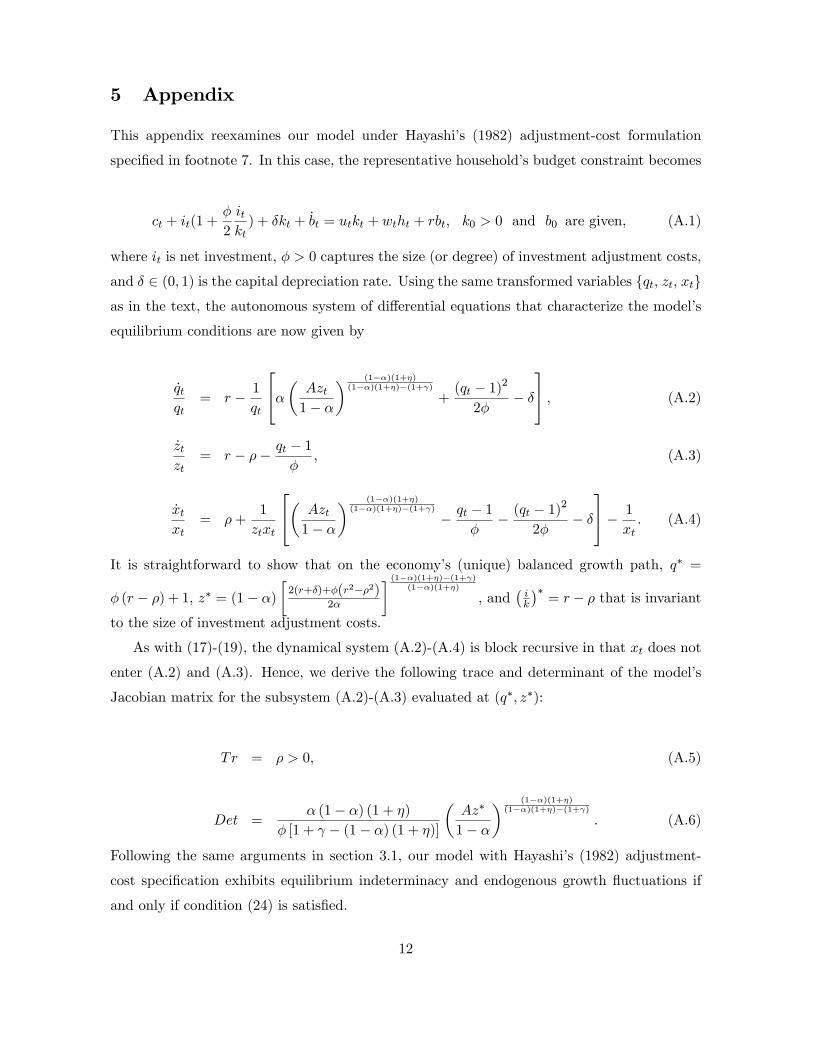
5 Appendix

This appendix reexamines our model under Hayashi’s (1982) adjustment-cost formulation

specified in footnote 7. In this case, the representative household’s budget constraint becomes

ct + it(1 +φ

2

itkt

) + δkt + bt = utkt + wtht + rbt, k0 > 0 and b0 are given, (A.1)

where it is net investment, φ > 0 captures the size (or degree) of investment adjustment costs,

and δ ∈ (0, 1) is the capital depreciation rate. Using the same transformed variables {qt, zt, xt}as in the text, the autonomous system of differential equations that characterize the model’s

equilibrium conditions are now given by

qtqt

= r − 1

qt

α( Azt1− α

) (1−α)(1+η)(1−α)(1+η)−(1+γ)

+(qt − 1)2

2φ− δ

, (A.2)

ztzt

= r − ρ− qt − 1

φ, (A.3)

xtxt

= ρ+1

ztxt

( Azt1− α

) (1−α)(1+η)(1−α)(1+η)−(1+γ)

− qt − 1

φ− (qt − 1)2

2φ− δ

− 1

xt. (A.4)

It is straightforward to show that on the economy’s (unique) balanced growth path, q∗ =

φ (r − ρ) + 1, z∗ = (1− α)

[2(r+δ)+φ(r2−ρ2)

2α

] (1−α)(1+η)−(1+γ)(1−α)(1+η)

, and(ik

)∗= r− ρ that is invariant

to the size of investment adjustment costs.

As with (17)-(19), the dynamical system (A.2)-(A.4) is block recursive in that xt does not

enter (A.2) and (A.3). Hence, we derive the following trace and determinant of the model’s

Jacobian matrix for the subsystem (A.2)-(A.3) evaluated at (q∗, z∗):

Tr = ρ > 0, (A.5)

Det =α (1− α) (1 + η)

φ [1 + γ − (1− α) (1 + η)]

(Az∗

1− α

) (1−α)(1+η)(1−α)(1+η)−(1+γ)

. (A.6)

Following the same arguments in section 3.1, our model with Hayashi’s (1982) adjustment-

cost specification exhibits equilibrium indeterminacy and endogenous growth fluctuations if

and only if condition (24) is satisfied.

12

References[1] Aguiar-Conraria, Luís and Yi Wen (2008), “A Note on Oil Dependence and Economic

Instability,”Macroeconomic Dynamics 12, 717-723.

[2] Benhabib, Jess and Roger E.A. Farmer (1994), “Indeterminacy and Increasing Returns,”Journal of Economic Theory 63, 19-41.

[3] Benhabib, Jess and Roger E.A. Farmer (1999), “Indeterminacy and Sunspots in Macro-economics,” in J. Taylor and M. Woodford, eds., Handbook of Macroeconomics, Vol. 1,North Holland: Amsterdam, 387-448.

[4] Chen, Yan and Yan Zhang (2009), “A Note on Tariff Policy, Increasing Returns, andEndogenous Fluctuations,”forthcoming in Macroeconomic Dynamics.

[5] Georges, Christophre (1995), “Adjustment Costs and Indeterminacy in Perfect ForesightModels,”Journal of Economic Dynamics and Control 19, 39-50.

[6] Guo, Jang-Ting and Kevin J. Lansing (2002), “Fiscal Policy, Increasing Returns, andEndogenous Fluctuations,”Macroeconomic Dynamics 6, 633-664.

[7] Guo, Jang-Ting and Kevin J. Lansing (2003), “Globally-Stabilizing Fiscal Policy Rules,”Studies in Nonlinear Dynamics & Econometrics 7, Issue 2, Article 3, 1-13.

[8] Hayashi, Fumio (1982), “Tobin’s Marginal q, Average q: A Neoclassical Interpretation,”Econometrica 50, 213-224.

[9] Herrendorf, Bethold and Ákos Valentinyi (2003), “Determinacy through IntertemporalCapital Adjustment Costs,”Review of Economic Dynamics 6, 483-497.

[10] Kim, Jinill (2003), “Indeterminacy and Investment Adjustment Costs: An AnalyticalResult,”Macroeconomic Dynamics 7, 394-406.

[11] Lahiri, Amartya (2001), “Growth and Equilibrium Indeterminacy: The Role of CapitalMobility,”Economic Theory 17, 197-208.

[12] Lucas, Robert E. Jr. and Edward C. Prescott (1971), “Investment under Uncertainty,”Econometrica, 39, 659-681.

[13] Meng, Qinglai and Andrés Velasco (2003), “Indeterminacy in a Small Open Economywith Endogenous Labor Supply,”Economic Theory 22, 661-669.

[14] Meng, Qinglai and Andrés Velasco (2004), “Market Imperfections and the Instability ofOpen Economies,”Journal of International Economics 64, 503-519.

[15] Turnovsky, Stephen J. (2002), “Knife-Edge Conditions and the Macroeconomics of SmallOpen Economies,”Macroeconomic Dynamics 6, 307-335.

[16] Weder, Mark (2001), “Indeterminacy in a Small Open Economy Ramsey Growth Model,”Journal of Economic Theory 98, 339-356.

[17] Wen, Yi (1998), “Indeterminacy, Dynamic Adjustment Costs, and Cycles,”EconomicsLetters 59, 213-216.

13