On the Inverse Problem of Binocular 3D MotionPerceptionMartin Lages*, Suzanne Heron

School of Psychology, University of Glasgow, Glasgow, Scotland

Abstract

It is shown that existing processing schemes of 3D motion perception such as interocular velocity difference, changingdisparity over time, as well as joint encoding of motion and disparity, do not offer a general solution to the inverse opticsproblem of local binocular 3D motion. Instead we suggest that local velocity constraints in combination with binoculardisparity and other depth cues provide a more flexible framework for the solution of the inverse problem. In the context ofthe aperture problem we derive predictions from two plausible default strategies: (1) the vector normal prefers slow motionin 3D whereas (2) the cyclopean average is based on slow motion in 2D. Predicting perceived motion directions forambiguous line motion provides an opportunity to distinguish between these strategies of 3D motion processing. Ourtheoretical results suggest that velocity constraints and disparity from feature tracking are needed to solve the inverseproblem of 3D motion perception. It seems plausible that motion and disparity input is processed in parallel and integratedlate in the visual processing hierarchy.

Citation: Lages M, Heron S (2010) On the Inverse Problem of Binocular 3D Motion Perception. PLoS Comput Biol 6(11): e1000999. doi:10.1371/journal.pcbi.1000999

Editor: Laurence T. Maloney, New York University, United States of America

Received March 23, 2010; Accepted October 14, 2010; Published November 18, 2010

Copyright: � 2010 Lages, Heron. This is an open-access article distributed under the terms of the Creative Commons Attribution License, which permitsunrestricted use, distribution, and reproduction in any medium, provided the original author and source are credited.

Funding: ML is supported by ESRC/MRC RES-060-25-0010 (UK) and SH is supported by an EPSRC studentship (UK). The funders had no role in study design,collection and analysis, decision to publish, or preparation of the manuscript.

Competing Interests: The authors have declared that no competing interests exist.

* E-mail: m.lages@psy.gla.ac.uk

Introduction

The representation of the three-dimensional (3D) external world

from two-dimensional (2D) retinal input is a fundamental problem

that the visual system has to solve [1–4]. This is true for static

scenes in 3D as well as for dynamic events in 3D space. For the

latter the inverse problem extends to the inference of dynamic

events in a 3D world from 2D motion signals projected into the left

and right eye. In the following we exclude observer movements

and only consider passively observed motion.

Velocity in 3D space is described by motion direction and speed.

Motion direction can be measured in terms of azimuth and

elevation angle, and motion direction together with speed is

conveniently expressed as a 3D motion vector in a cartesian

coordinate system. Estimating such a vector locally is highly

desirable for a visual system because the representation of local

estimates in a dense vector field provides the basis for the perception

of 3D object motion, that is direction and speed of moving objects.

This information is essential for interpreting events as well as

planning and executing actions in a dynamic environment.

If a single moving point, corner or other unique feature serves as

binocular input then intersection of constraint lines or triangula-

tion together with a starting point provides a straightforward and

unique geometrical solution to the inverse problem in a binocular

viewing geometry (see Methods and Fig. 1 for an illustration). If,

however, the moving stimulus has spatial extent, such as an edge,

contour, or line inside a circular aperture [5] then local motion

direction in corresponding receptive fields of the left and right eye

remains ambiguous and additional constraints are needed to solve

the aperture and inverse problem in 3D.

The inverse optics and the aperture problem are well-known

problems in computational vision, especially in the context of

stereo [3,6], structure from motion [7], and optic flow [8].

Gradient constraint methods belong to the most widely used

techniques of optic-flow computation from image sequences. They

can be divided into local area-based [9] and into more global optic

flow methods [10]. Both techniques employ brightness constancy

and smoothness constraints in the image to estimate velocity in an

over-determined equation system. It is important to note that

optical flow only provides a constraint in the direction of the image

gradient, the normal component of the optical flow. As a

consequence some form of regularization or smoothing is needed.

Similar techniques in terms of error minimization and

regularization have been offered for 3D stereo-motion detection

[11–13]. Essentially these algorithms extend processing principles

of 2D optic flow to 3D scene flow.

Computational studies on 3D motion algorithms are usually

concerned with fast and efficient encoding when tested against

ground truth. Here we are less concerned with the efficiency or

robustness of a particular implementation. Instead we want to

understand and predict behavioral characteristics of human 3D

motion perception. 2D motion perception has been extensively

researched in the context of the 2D aperture problem [14–16] but

there is a surprising lack of studies on the aperture problem and

3D motion perception.

Any physiologically plausible solution to the inverse 3D motion

problem has to rely on binocular sampling of local spatio-temporal

information. There are at least three known cell types in early

visual cortex that may be involved in local encoding of 3D motion:

simple and complex motion detecting cells [17–20], binocular

PLoS Computational Biology | www.ploscompbiol.org 1 November 2010 | Volume 6 | Issue 11 | e1000999

disparity detecting cells [21] sampled over time, and joint motion

and disparity detecting cells [22–24].

It is therefore not surprising that three approaches to binocular

3D motion perception have emerged in the literature: Interocular

velocity difference (IOVD), changing disparity over time (CDOT),

and joint encoding of motion and disparity (JEMD).

These three approaches have generated an extensive body of

research but psychophysical results have been inconclusive and the

nature of 3D motion processing remains an unresolved issue

[25,26]. Despite the wealth of empirical studies on motion in depth

there is a lack of studies on true 3D motion stimuli. Previous

psychophysical and neurophysiological studies typically employ

stimulus dots with unambiguous motion direction or fronto-

parallel random-dot surfaces moving in depth. The aperture

problem and local motion encoding however, which features so

prominently in 2D motion perception [14–16] has been neglected

in the study of 3D motion perception.

Large and persistent perceptual bias has been found for dot

stimuli with unambiguous motion direction [27–29] suggesting

processing strategies that are different from the three main

processing models [28–30]. It seems promising to investigate local

motion stimuli with ambiguous motion direction such as a line or

contour moving inside a circular aperture [31] because they relate

to local encoding [17–24] and may reveal principles of 3D motion

processing [32].

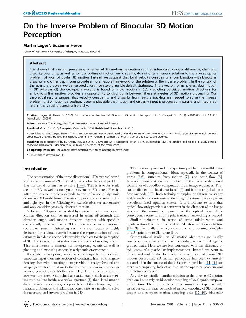
Figure 1. Illustration of the aperture problem of 3D motion with projections of an oriented line or contour moving in depth. The leftand right eye with nodal points a and c, separated by interocular distance i, are verged on a fixation point F at viewing distance D. If an orientedstimulus (diagonal line) moves from the fixation point to a new position in depth along a known trajectory (black arrow) then perspective projectionof the line stimulus onto local areas on the retinae or a fronto-parallel screen creates 2D aperture problems for the left and right eye (green andbrown arrows).doi:10.1371/journal.pcbi.1000999.g001

Author Summary

Humans and many other predators have two eyes that areset a short distance apart so that an extensive region ofthe world is seen simultaneously by both eyes fromslightly different points of view. Although the images ofthe world are essentially two-dimensional, we vividly seethe world as three-dimensional. This is true for static aswell as dynamic images. Here we elaborate on how thevisual system may establish 3D motion perception fromlocal input in the left and right eye. Using tools fromanalytic geometry we show that existing 3D motionmodels offer no general solution to the inverse opticsproblem of 3D motion perception. We suggest a flexibleframework of motion and depth processing and suggestdefault strategies for local 3D motion estimation. Ourresults on the aperture and inverse problem of 3D motionare likely to stimulate computational, behavioral, andneuroscientific studies because they address the funda-mental issue of how 3D motion is represented in the visualsystem.

Inverse Problem of 3D Motion

PLoS Computational Biology | www.ploscompbiol.org 2 November 2010 | Volume 6 | Issue 11 | e1000999

The aim of this paper is to evaluate existing models of 3D

motion perception and to gain a better understanding of binocular

3D motion perception. First, we show that existing models of 3D

motion perception are insufficient to solve the inverse problem of

binocular 3D motion. Second, we establish velocity constraints in

a binocular viewing geometry and demonstrate that additional

information is necessary to disambiguate local velocity constraints

and to derive a velocity estimate. Third, we compare two default

strategies of perceived 3D motion when local motion direction is

ambiguous. It is shown that critical stimulus conditions exist that

can help to determine whether 3D motion perception favors slow

3D motion or averaged cyclopean motion.

Results

In the following we summarize shortcomings for each of the

three main approaches to binocular 3D motion perception in

terms of stereo and motion correspondence, 3D motion direction,

and speed. We also provide a counterexample to illustrate the

limitations of each approach.

Interocular velocity difference (IOVD)This influential processing model assumes that monocular

spatio-temporal differentiation or motion detection [33] is

followed by a difference computation between velocities in the

left and right eye [34–36]. The difference or ratio between

monocular motion vectors in each eye, usually in a viewing

geometry where interocular separation i and viewing distance D is

known, provides an estimate of motion direction in terms of

azimuth angle only.

We argue that the standard IOVD model [29,37–40] is

incomplete and ill-posed if we consider local motion encoding

and the aperture problem. In the following the limitations of the

IOVD model are illustrated.

Stereo correspondence. The first limitation is easily

overlooked: IOVD assumes stereo correspondence between

motion in the left and right eye when estimating 3D motion

trajectory. The model does not specify which motion vector in the

left eye should correspond to which motion vector in the right eye

before computing a velocity difference. If there is only a single

motion vector in the left and right eye then establishing a stereo

correspondence appears trivial since there are only two positions

in the left and right eye that signal dynamic information.

Nevertheless, stereo correspondence is a necessary pre-requisite

of IOVD processing which quickly becomes challenging if we

consider multiple stimuli that excite not only one but many local

motion detectors in the left and right eye. It is concluded that

without explicit stereo correspondence between local motion

detectors the IOVD model is incomplete.

3D motion direction. The second problem concerns 3D

motion trajectories with arbitrary azimuth and elevation angles.

Consider a local contour with spatial extent such as an oriented

line inside a circular aperture so that the endpoints of the line are

occluded. This is known as the aperture problem in stereopsis

[5,41]. If an observer maintains fixation at close or moderate

viewing distance then the oriented line stimulus projects differently

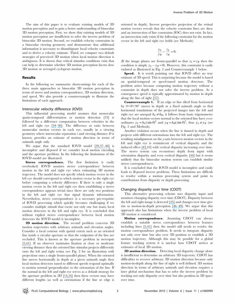
onto the left and right retina (see Fig. 2 for an illustration with

projections onto a single fronto-parallel plane). When the oriented

line moves horizontally in depth at a given azimuth angle then

local motion detectors tuned to different speeds respond optimally

to motion normal (perpendicular) to the orientation of the line. If

the normal in the left and right eye serves as a default strategy for

the aperture problem in 2D [14,16] then these vectors may have

different lengths (as well as orientations if the line or edge is

oriented in depth). Inverse perspective projection of the retinal

motion vectors reveals that the velocity constraint lines are skew

and an intersection of line constraints (IOC) does not exist. In fact,

an intersection only exists if the following constraint for the motion

vector in the left and right eye holds (see Methods):

yL

yR

{zL

zR

~0:

(If the image planes are fronto-parallel so that zL~zR then the

condition is simply yL{yR~0). However, this constraint is easily

violated as illustrated in Fig. 2 and Counterexample 1 below.

Speed. It is worth pointing out that IOVD offers no true

estimate of 3D speed. This is surprising because the model is based

on spatial-temporal or speed-tuned motion detectors. The

problem arises because computing motion trajectory without a

constraint in depth does not solve the inverse problem. As a

consequence speed is typically approximated by motion in depth

along the line of sight [37].

Counterexample 1. If an edge or line tilted from horizontal

by 0,h,90u moves in depth at a fixed azimuth angle so that

horizontal translations of the projected images into the left and

right eye are unequal hL=hR, it follows from basic trigonometry

that the local motion vectors normal to the oriented line have y-co-

ordinates yL~hL( sin h)2 and yR~hR( sin h)2, thus yL=yR (see

Fig. 2 and Methods).

Another violation occurs when the line is slanted in depth and

projects with different orientations into the left and right eye. The

resulting misalignment on the y-axis between motion vectors in the

left and right eye is reminiscent of vertical disparity and the

induced effect [42,43] with vertical disparity increasing over time.

The stereo system can reconstruct depth from input with

orientation disparity and even vertical disparity [44] but it seems

unlikely that the binocular motion system can establish similar

stereo correspondences.

It is concluded that the IOVD model is incomplete and easily

leads to ill-posed inverse problems. These limitations are difficult

to resolve within a motion processing system and point to

contributions from disparity or depth processing.

Changing disparity over time (CDOT)This alternative processing scheme uses disparity input and

monitors changing disparity over time (CDOT). Disparity between

the left and right image is detected [45] and changes over time give

rise to motion-in-depth perception [46–49]. We argue that this

approach also has limitations when the inverse problem of local

3D motion is considered.

Motion correspondence. Assuming CDOT can always

establish a suitable stereo correspondence between features

including lines [5,41] then the model still needs to resolve the

motion correspondence problem. It needs to integrate disparity

not only over time but also over 3D position to establish a 3D

motion trajectory. Although this may be possible for a global

feature tracking system it is unclear how CDOT arrives at

estimates of local 3D motion.

3D motion direction. Detecting local disparity change alone

is insufficient to determine an arbitrary 3D trajectory. CDOT has

difficulties to recover arbitrary 3D motion direction because only

motion-in-depth along the line of sight is well defined. 3D motion

direction in terms of arbitrary azimuth and elevation requires a

later global mechanism that has to solve the inverse problem by

tracking not only disparity over time but also position in 3D space

over time.

Inverse Problem of 3D Motion

PLoS Computational Biology | www.ploscompbiol.org 3 November 2010 | Volume 6 | Issue 11 | e1000999

Speed. As a consequence the rate of change of disparity

provides a speed estimate for motion-in-depth along the line of

sight but not for arbitrary 3D motion trajectories.

Counterexample 2. In the context of local surface motion

consider a horizontally slanted surface moving to the left or right

behind a circular aperture. Without corners or other unique

features CDOT can only detect local motion in depth along the

line of sight. Similarly in the context of local line motion, the

inverse problem remains ill posed for a local edge or line moving

on a slanted surface because additional motion constraints are

needed to determine a 3D motion direction.

In summary, CDOT does not provide a general solution to the

inverse problem of local 3D motion because it lacks information

on motion direction. Even though CDOT is capable of extracting

stereo correspondences over time, additional motion constraints

are needed to represent arbitrary motion trajectories in 3D space.

Joint encoding of motion and disparity (JEMD)This approach postulates that early binocular cells are both

motion and disparity selective and physiological evidence for the

existence of such cells was found in cat striate cortex [22] and

monkey V1 [50] (see however [51]). Model cells in this hybrid

approach extract motion and disparity energy from local

stimulation. A read-out from population activity and population

decoding is needed to explain global 3D motion phenomena such

as transparent motion and Pulfrich-like effects [52,53]. Although

JEMD is physiologically plausible it shares two problems with

IOVD.

3D motion direction. Similar to cells tuned to binocular

motion, model cells of JEMD prefer corresponding velocities in the

left and right eye. Therefore a binocular model cell can only

establish a 2D fronto-parallel velocity constraint at a given depth.

Model cell activity remains ambiguous because it can be the result

of local disparity or motion input [54]. A later processing stage,

possibly at the level of human V5/MT [55] needs to read out

population cell activities across positions and depth planes and has

to approximate global 3D motion. Similar to CDOT, the model

defers the inverse problem to a later global processing stage.

Speed. Again, similar to IOVD and CDOT, JEMD provides

no local 3D speed estimate. It also has to rely on sampling across

depth planes in a population of cells in order to approximate

speed.

Counterexample 3. Consider local 3D motion with unequal

velocities in the left and right eye but the same average velocity,

e.g. diagonal trajectories to the front and back through the same

point in depth. JEMD has no mechanism to discriminate between

these local 3D trajectories when monitoring binocular cell activity

across depth planes in a given temporal window.

In the following we introduce general velocity constraints for 3D

motion and suggest two default strategies of 3D motion perception

that are based on different processing principles (see Methods for

details).

Figure 2. Inverse projection of constraint lines preferring slow 2D motion in the left and right eye. Constraint lines through projectionpoint b and d do not intersect and 3D motion cannot be determined (see text for details).doi:10.1371/journal.pcbi.1000999.g002

Inverse Problem of 3D Motion

PLoS Computational Biology | www.ploscompbiol.org 4 November 2010 | Volume 6 | Issue 11 | e1000999

Velocity constraints and two default strategiesWhich constraints does the visual system use to solve the inverse

as well as aperture problem for local 3D line motion where

endpoints are invisible or occluded? This is a critical question

because it is linked to local motion encoding and the possible

contribution from depth processing.

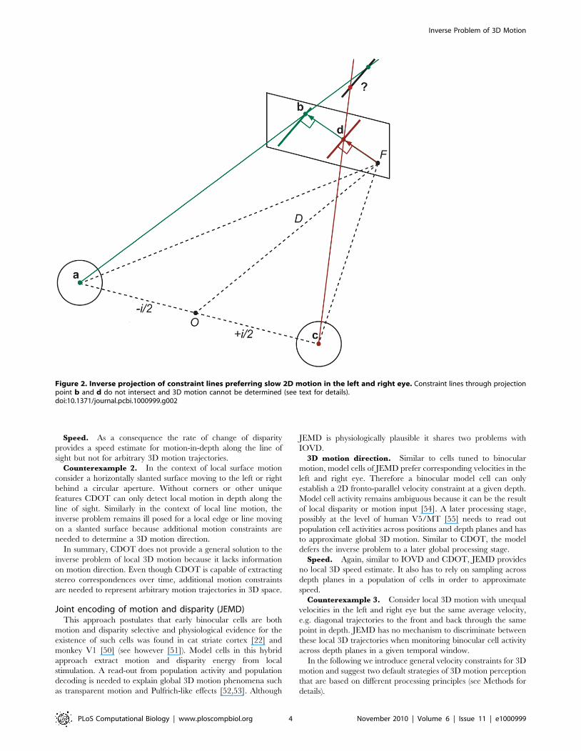
The 3D motion system may establish constraint planes rather

than constraint lines to capture all possible motion directions of a

contour or edge, including motion in the direction of the edge’s

orientation. Geometrically the intersection of two constraint planes

in a given binocular viewing geometry defines a constraint line

oriented in 3D velocity space (see Fig. 3 and Methods).

We suggest that in analogy to 2D motion perception [15,56]

tracking of features in depth coupled with binocular velocity

constraints from motion processing provides a flexible strategy to

disambiguate 3D motion direction and to solve the inverse

problem of 3D motion perception.

But which principles or constraints are used? Does the binocular

motion system prefer slow 3D motion or averaged 2D motion?

Does it solve stereo correspondence before establishing binocular

velocity constraints or does it average 2D velocity constraints from

the left and right eye before it solves stereo correspondence? We

derive predictions for two alternative strategies to address these

questions.

Vector normal (VN). Velocity constraints in the left and

right eye provide velocity constraint planes in 3D velocity space. In

Fig. 3 they are illustrated as translucent green and brown triangles

in a binocular viewing geometry. The intersection of constraint

planes defines a velocity constraint line in 3D that also describes

the true end-position of the moving line or contour (black line).

The vector or line normal from the oriented constraint line to the

starting point gives a default 3D motion estimate (blue arrow). It is

the shortest distance in 3D velocity space and denotes the slowest

motion vector that fulfills both constraints. Note that this strategy

requires that the 3D motion system has established some stereo

correspondence so that the intersection of constraints as well as the

vector normal can be found in 3D velocity space.

The VN strategy is a generalization of the vector normal and

IOC in 2D [15] and it is related to area-based regression and

gradient constraint models [9] where the local brightness

constancy constraint ensures a default solution that is normal to

the orientation of image intensity.

Cyclopean average (CA). If the motion system computes

slow 2D motion independently in the left and right eye then the

cyclopean average provides an alternative velocity constraint

[27,57]. Averaging of monocular constraints increases robustness

of the motion signal at the expense of binocular disparity

information. Thus, a cyclopean average constrains velocity but

gives no default estimate of velocity. However, if we attach

(dynamic) disparity to the cyclopean average then the CA provides

a default estimate of 3D velocity (see Methods and Fig. 4).

The CA strategy is a generalized version of the vector average

strategy for 2D motion [58] and can be linked to computational

models of 3D motion that use global gradient and smoothness

constraints [10]. These global models amount to computing the

average flow vector in the neighborhood of each point and refining

Figure 3. Illustration of vector normal (VN) as a default strategy for local 3D motion perception (see text for details). The intersectionof constraint planes (IOC) together with the assumption of slow motion describes the shortest vector in 3D space (blue arrow) that fulfills the velocityconstraints.doi:10.1371/journal.pcbi.1000999.g003

Inverse Problem of 3D Motion

PLoS Computational Biology | www.ploscompbiol.org 5 November 2010 | Volume 6 | Issue 11 | e1000999

the scene flow vector by the residual of the average flow vectors in

the neighborhood. Interestingly, tracking the two intersection

points or T junctions of a moving line with a circular aperture in

the left and right eye and averaging the resulting vectors gives

predictions that are equivalent to the CA strategy.

Predictions for VN and CA strategy. We use the Vector

Normal (VN) and Cyclopean Average (CA) as default strategies to

predict 3D velocity of an oriented line or contour moving in depth

inside a circular aperture.

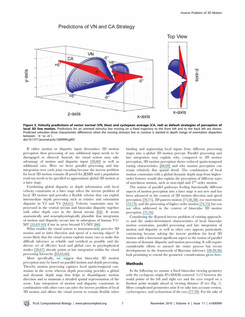
The 3D plot in Fig. 5 shows predictions of the VN strategy

(blue) and the CA strategy (red) for a diagonal line stimulus moving

on two trajectories in depth at a viewing distance D = 57 cm and

interocular distance of i = 6.5 cm. The line stimulus has a

trajectory to the front and left with azimuth +57.2 deg and

elevation 0 deg, and a trajectory to the back and left with azimuth

257.2 deg and elevation 0 deg. Azimuth and elevation of 0 deg

denotes a horizontal and fronto-parallel trajectory to the left. The

starting point of each trajectory is the origin of the vector fields in

the 3D plot. An open circle denotes the endpoint of a predicted

motion vector. For each default strategy and stimulus trajectory a

field of 120 vectors are shown with orientation disparity of the line

stimulus ranging from 26u to +6u in steps of 0.1u. Orientation

disparity changes perceived slant of the diagonal line so that at

26u the bottom-half of the line is slanted away from the observer

and the top-half is slanted towards the observer.

If the diagonal line is fronto-parallel and has zero orientation

disparity both strategies make equivalent predictions (intersection

of red and blue vector fields in Fig. 5). If, however, the stimulus

line has orientation disparity and is slanted in depth then

predictions clearly discriminate between the two strategies. The

VN strategy always finds the shortest vector between starting point

and moving line so that velocity predictions approximate a semi-

circle for changing orientation disparity. Please note that for the

VN predictions the sign of orientation disparity reverses for the

stimulus trajectory to the front and back. The CA strategy on the

other hand computes an average vector and as a consequence the

endpoints of the predictions approximate a velocity constraint line

through the cyclopean origin.

In a first experiment using a psychophysical matching task we

measured the perceived 3D motion direction of an oriented line

moving behind a circular aperture. Preliminary results from four

observers indicate VN as the default strategy. Perceptual bias from

depth processing reduced perceived slant of the stimulus line and

this also affected motion direction [30].

Discussion

IOVD and CDOT are extreme models because they are based on

either motion or disparity input. IOVD excludes contributions from

binocular disparity processing but requires early stereo correspon-

dence. It does not solve the inverse problem for local 3D line motion

because it is confined to 3D motion in the x- or z-plane.

CDOT on the other hand excludes contributions from motion

processing and therefore has problems to establish motion

correspondence and direction. Without further assumptions it is

confined to motion in depth along the line of sight.

Figure 4. Illustration of cyclopean average (CA) as a default strategy for local 3D motion perception (see text for details). Combiningthe cyclopean velocity constraint with horizontal disparity determines a vector in 3D space (red arrow) with average monocular velocity.doi:10.1371/journal.pcbi.1000999.g004

Inverse Problem of 3D Motion

PLoS Computational Biology | www.ploscompbiol.org 6 November 2010 | Volume 6 | Issue 11 | e1000999

If either motion or disparity input determines 3D motion

perception then processing of any additional input needs to be

disengaged or silenced. Instead, the visual system may take

advantage of motion and disparity input [59,60] as well as

additional cues. Here we favor parallel processing and late

integration over early joint encoding because the inverse problem

for local 3D motion remains ill posed for JEMD and a population

read-out needs to be specified to approximate global 3D motion at

a later stage.

Combining global disparity or depth information with local

velocity constraints at a later stage solves the inverse problem of

local 3D motion and provides a flexible scheme that can exploit

intermediate depth processing such as relative and orientation

disparity in V2 and V4 [44,61]. Velocity constraints may be

processed in the ventral stream and binocular disparity together

with other depth cues in the dorsal stream [62]. It seems

anatomically and neurophysiologically plausible that integration

of motion and disparity occurs late in subregions of human V5/

MT [55,63–65] if not in areas beyond V5/MT [66].

What enables the visual system to instantaneously perceive 3D

motion and to infer direction and speed of a moving object? It

seems likely that the visual system exploits many cues to make this

difficult inference as reliable and veridical as possible and the

diverse set of effective local and global cues in psychophysical

studies [59,67] already points at late integration within the visual

processing hierarchy [62,65,66].

More specifically, we suggest that binocular 3D motion

perception may be based on parallel motion and depth processing.

Thereby motion processing captures local spatio-temporal con-

straints in the scene whereas depth processing provides a global

and dynamic depth map that helps to disambiguate motion

direction and to maintain a detailed spatial representation of the

scene. Late integration of motion and disparity constraints in

combination with other cues can solve the inverse problem of local

3D motion and allows the visual system to remain flexible when

binding and segmenting local inputs from different processing

stages into a global 3D motion percept. Parallel processing and

late integration may explain why, compared to 2D motion

perception, 3D motion perception shows reduced spatio-temporal

tuning characteristics [68,69] and why motion perception can

retain relatively fine spatial detail. The combination of local

motion constraints with a global dynamic depth map from higher-

order features would also explain the perception of different types

of non-linear motion, such as non-rigid and 2nd order motion.

The notion of parallel pathways feeding functionally different

aspects of motion perception into a later stage is not new and has

been advanced in the context of 2D motion direction and speed

perception [70,71], 2D pattern motion [15,56,58], eye movements

[72,73], and the processing of higher order motion [74,75] but was

not often addressed in the context of binocular 3D motion

perception [75,76].

Considering the ill-posed inverse problem of existing approach-

es and the under-determined characteristics of local binocular

motion constraints, parallel processing and late integration of

motion and disparity as well as other cues appears particularly

convincing because solving the inverse problem for local 3D

motion adds a functional significant aspect to the notion of parallel

streams of dynamic disparity and motion processing. It will require

considerable efforts to unravel the entire process but recent

developments in the framework of Bayesian inference [28,29,56]

look promising to extend the geometric considerations given here.

Methods

In the following we assume a fixed binocular viewing geometry

with the cyclopean origin O~(0,0,0) centered 6i/2 between the

nodal points of the left and right eye and the eyes verged on a

fixation point straight ahead at viewing distance D (see Fig. 1).

More complicated geometries arise if we take into account version,

cyclovergence, and cyclotorsion of the eyes [77,78]. For the sake of

Figure 5. Velocity predictions of vector normal (VN, blue) and cyclopean average (CA, red) as default strategies of perception oflocal 3D line motion. Predictions for an oriented stimulus line moving on a fixed trajectory to the front left and to the back left are shown.Predicted velocities show characteristic differences when the moving stimulus line or contour is slanted in depth (range of orientation disparitiesbetween 26u to +6u).doi:10.1371/journal.pcbi.1000999.g005

Inverse Problem of 3D Motion

PLoS Computational Biology | www.ploscompbiol.org 7 November 2010 | Volume 6 | Issue 11 | e1000999

simplicity we ignore the non-linear aspects of visual space [79] and

represent perceived 3D motion as a linear vector in a three-

dimensional Euclidean space where the fixation point is also the

starting point of the motion stimulus.

Since we are not concerned about particular algorithms and

their implementation, results are given in terms of analytic

geometry [80,81].

Intersection of constraint linesIf the eyes remain verged on a fixation point in a binocular

viewing geometry then the constraint line in the left and right eye

can be defined by pairs of points a,bð Þ and c,dð Þ, respectively. The

nodal point in the left eye a~ {i=2,0,0ð Þ and a projection point

b~ xL,yL,zLð Þ of the motion vector on the left retina define a

constraint line for the left eye. Similarly, points c~ zi=2,0,0ð Þ and

d~ xR,yR,zRð Þ determine a constraint line in the right eye. The

corresponding vector directions are given by

a{cð Þ~ {i=2,0,0ð Þ{ zi=2,0,0ð Þ~ {i,0,0ð Þ

b{að Þ~ xL,yL,zLð Þ{ {i=2,0,0ð Þ~ xLzi=2,yL,zLð Þ

d{cð Þ~ xR,yR,zRð Þ{ zi=2,0,0ð Þ~ xR{i=2,yR,zRð Þ

ð1Þ

Each constraint line can expressed by a pair of points a,bð Þ and

c,dð Þ together with scalar t:

xL~az b{að Þ t

xR~cz d{cð Þ tð2Þ

The two lines intersect for

t~½(c{a)|(d{c)�:½(b{a)|(d{c)�

(b{a)|(d{c)k k2ð3Þ

if and only if

a{cð Þ: b{að Þ| d{cð Þ½ �~0 ð4Þ

where : is the scalar product also called the dot product,6denotes

the cross product, and . . .k k the norm of a vector. Otherwise, the

two lines are skew, and the inverse problem is ill posed.

We can exclude the trivial case a{cð Þ~0 because the two eyes

are separated by iw0. We also exclude the special case where the

cross product is zero because the motion vectors in the left and

right eye are identical or opposite.

The cross product in (4) can be written as

b{að Þ| d{cð Þ~

yLzR{zLyR,zL(xR{i=2){(xLzi=2) zR,(xLzi=2) yR{yL (xR{i=2)ð Þð5Þ

Since a{cð Þ~ {i,0,0ð Þ in Eq. (4) we are only concerned with the

product {i yLzR{zLyRð Þ which equals zero if and only if

yLzR~yRzL oryL

yR

{zL

zR

~0, ð6Þ

The ratio of z co-ordinates on the right-hand side may be different

from 1 as a result of eye vergence and the left-hand side reflects the

corresponding ratio of vertical displacements.

In the following we consider the simpler case of projections onto

a fronto-parallel screen (coplanar retinae) at a fixed viewing

distance D (see Fig. 2). In this case epipolar lines are horizontal

with equivalent co-ordinates zL~zR~zC on the z-axis.

Again, since a{cð Þ~ {i,0,0ð Þ in (4) we only have to evaluate

{izC(yL{yR) which is zero if and only if:

yL{yR~0 ð7Þ

For an intersection to exist the left and right eye motion vector

must have equivalent horizontal y co-ordinates or zero vertical

disparity.

Intersection of constraint planesMonocular line motion defines a constraint plane with three

points: the nodal point of an eye and two points defining the end

position of the projected line (see Fig. 3). In order to find the

intersection of the left and right eye constraint plane we use the

plane normal in the left and right eye. If the two planes are

specified in Hessian normal form

nL:p~dL,

nR:p~dR

ð8Þ

where : is again the dot product, n~(a,b,c) is a vector describing

the surface normal to a plane, p~(x,y,z) is a vector representing

all points on the plane, and d is a scalar.

We need to check whether the constraint planes are parallel or

coincident, that is if

nL|nR~0 ð9Þ

before we can determine their intersection. The equation for the

intersection of the two constraint planes is a line here written as

p~cLnLzcRnRzu(nL|nR) ð10Þ

where u is a free parameter. Taking the dot product of the above

with each plane normal gives two equations with unknown scalars

cL and cR.

nL:p~dL~cL(nL

:nL)zcR(nL:nR)

nR:p~dR~cL(nL

:nR)zcR(nR:nR)

ð11Þ

Solving the two equations for cL and cR gives

cL~½dL(nR:nR){dR(nL

:nR)�=D,

cR~½dR(nL:nL){dR(nL

:nR�=D

where D~(nL:nL) (nR

:nR){(nL:nR)2:

ð12Þ

Inserting cL and cR in (10) determines the intersection of constraints

or constraint line p.

In analogy to the 2D aperture problem and the intersection of

constraints we can now define two plausible strategies for solving

the 3D aperture problem:

Vector normal (VN)The shortest distance in 3-D (velocity) space between the

starting point p0~(0,0,D) of the stimulus line and the constraint

line p is the line or vector normal through point p0. In order to

determine the intersection point of the vector normal with the

ð5Þ

Inverse Problem of 3D Motion

PLoS Computational Biology | www.ploscompbiol.org 8 November 2010 | Volume 6 | Issue 11 | e1000999

constraint line we pick two arbitrary points p1 and p2 on

intersection constraint line p by choosing a scalar u (e.g., 0.5).

p1~cLnLzcRnR{u(nL|nR)

p2~cLnLzcRnRzu(nL|nR)ð13Þ

Together with point p0 we can compute scalar tn as

tn~{(p1{p0):(p2{p1)

p2{p1k k2ð14Þ

which determines the closest intersection point x on the constraint

line:

x~p1z p2{p1ð Þtn ð15Þ

Cyclopean average (CA)We can define a cyclopean constraint line in terms of the

cyclopean origin O~(0,0,0) and projection point pC~(xC ,yC ,zC)on a fronto-parallel screen where xC~(xLzxR)=2 and

yC~(yLzyR)=2 are the averages of the 2D normal co-ordinates

for the left and right eye projections.

If we measure disparity d at the same retinal coordinates as the

horizontal offset between the left and right eye anchored at

position pC then we can define new points b with x’L~xC{d=2and d with x’R~xCzd=2. (Alternatively, we may establish an

epipolar or more sophisticated disparity constraint.) The resulting

two points together with the corresponding nodal points a and cdefine two constraint lines as in (2), one for the left and the other

for the right eye. By inserting the new co-ordinates from above

into (4) it is easy to see that condition (6) holds and the scalar for

the intersection of lines can be found as in (3).

Transformation into spherical co-ordinatesThe intersection x~(x,y,z) in cartesian co-ordinates can be

transformed into spherical co-ordinates (a,b, sk k) using vectors

q~(x,0,z{D) and r~(x,0,D) to determine azimuth a in the

horizontal plane

a~ arccosq:r

qk k rk k

� �ð16Þ

Similarly, for base vectors s~(x,y,z{D) and q~(x,0,z{D)elevation b is given by

b~ arccoss:q

sk k qk k

� �ð17Þ

Speed in 3D space is equivalent to the norm of vector s written as

sk k.

Author Contributions

Conceived and designed the experiments: ML SH. Contributed reagents/

materials/analysis tools: ML SH. Wrote the paper: ML SH.

References

1. Berkeley G (1709/1975) Philosophical Works; Including the Works on Vision.In: M Ayers M, ed. London, Dent.

2. von Helmholtz H In: Southall JP, ed. Helmholtz’s Treatise on Physiological

Optics, Vol 1. Dover: New York, USA. pp 312–313.

3. Poggio T, Torre V, Koch C (1985) Computational vision and regularizationtheory. Nature 317: 314–319.

4. Pizlo Z (2001) Perception viewed as an inverse problem. Vision Res 41:

3145–3161.

5. Morgan MJ, Castet E (1997) The aperture problem in stereopsis. Vision Res 37:2737–2744.

6. Mayhew JEW, Longuet-Higgins HC (1982) A computational model of binocular

depth perception. Nature 297: 376–378.

7. Koenderink JJ, van Doorn AJ (1991) Affine structure from motion. J Opt SocAm 8: 377–385.

8. Hildreth EC (1984) The computation of the velocity field. Proc R Soc

Lond B Biol Sci 221: 189–220.

9. Lucas BD, Kanade T (1981) An Iterative Image Registration Technique with anApplication to Stereo Vision, DARPA Image Understanding Workshop, pp121–

130 (see also IJCAI’81, pp674–679).

10. Horn BKP, Schunck BG (1981) Determining optical flow. Artif Intell 17:185–203.

11. Spies H, Jahne BJ, Barron JL (2002) Range flow estimation. Comput Vis Image

Underst 85: 209–231.

12. Min D, Sohn K (2006) Edge-preserving simultaneous joint motion-disparityestimation. Proceedings of the 18th International Conference on Pattern

Recognition Vol 2: 74–77.

13. Scharr H, Kusters R (2002) A linear model for simultaneous estimation of 3Dmotion and depth. IEEE Workshop on Motion and Video Computing, Orlando

FL. pp 1–6.

14. Wallach H (1935) Uber visuell wahrgenommene Bewegungsrichtung. PsycholRes 20: 325–380.

15. Adelson EH, Movshon JA (1982) Phenomenal coherence of moving visual

patterns. Nature 300: 523–525.

16. Sung K, Wojtach WT, Purves D (2009) An empirical explanation of apertureeffects. Proc Nat Acad Sci USA 106: 298–303.

17. Hubel DH, Wiesel TN (1962) Receptive fields, binocular interaction and

functional architecture in the cat’s visual cortex. J Physiol (Lond.)160: 106–154.

18. Hubel DH, Wiesel TN (1968) Receptive fields and functional architecture ofmonkey striate cortex. J Physiol 195: 215–243.

19. DeAngelis GC, Ohzawa I, Freeman RD (1993) Spatiotemporal organization of

simple-cell receptive fields in the cat’s striate cortex. 1. General characteristics

and postnatal development. J Neurophys 69: 1091–1117.

20. Maunsell JH, van Essen DC (1983) Functional properties of neurons in middletemporal visual area of the macaque monkey: I. Selectivity for stimulus direction,

speed, and orientation. J Neurophys 49: 1127–1147.

21. Hubel DH, Wiesel TN (1970) Stereoscopic vision in macaque monkey. Cellssensitive to binocular depth in area 18 of the macaque monkey cortex. Nature

225: 41–42.

22. Anzai A, Ohzawa I, Freeman RD (2001) Joint encoding of motion and depth byvisual cortical neurons: neural basis of he Pulfrich effect. Nat Neurosci 4:

513–518.

23. Bradley DC, Qian N, Andersen RA (1995) Integration of motion and stereopsisin middle temporal cortical area of macaques. Nature 373: 609–611.

24. DeAngelis GC, Newsome WT (1999) Organization of disparity-selective neurons

in macaque area MT. J Neurosci 19: 1398–1415.

25. Regan D, Gray R (2009) Binocular processing of motion; some unresolvedproblems. Spatial Vision 22: 1–43.

26. Harris JM, Nefs HT, Grafton CE (2008) Binocular vision and motion-in-depth.

Spat Vis 21: 531–547.

27. Harris JM, Drga (2005) Using visual direction in three-dimensional motionperception. Nat Neurosci 8: 229–233.

28. Lages M (2006) Bayesian models of binocular 3-D motion perception. J Vision 6:

508–522.

29. Welchman AE, Lam JM, Bulthoff HH (2008) Bayesian motion estimationaccounts for a surprising bias in 3D vision. Proc Nat Acad Sci USA 105:

12087–92.

30. Ji H, Fermuller C (2006) Noise causes slant underestimation in stereo and

motion. Vision Res 46: 3105–3120.31. Heron S, Lages M (2009) Measuring azimuth and elevation of binocular 3D

motion direction [Abstract]. J Vision 9: 637a.

32. Lages M, Heron S (2009) Testing generalized models of binocular 3D motion

perception [Abstract]. J Vision 9: 636a.33. Adelson EH, Bergen JR (1985) Spatio-temporal energy models for the

perception of motion. J Opt Soc Am A 2: 284–299.

34. Beverley KI, Regan D (1973) Evidence for the existence of neural mechanisms

selectively sensitive to the direction of movement in space. J Physiol 235: 17–29.35. Beverley KI, Regan D (1975) The relation between discrimination and

sensitivity in the perception of motion in depth. J Physiol 249: 387–398.

36. Regan D, Beverley KI (1973) Some dynamic features of depth perception.

Vision Res 13: 2369–2379.37. Brooks KR (2002) Interocular velocity difference contributes to stereomotion

speed perception. J Vision 2: 218–231.

38. Shioiri S, Saisho H, Yaguchi H (2000) Motion in depth based on inter-ocular

velocity differences. Vision Res 40: 2565–2572.

Inverse Problem of 3D Motion

PLoS Computational Biology | www.ploscompbiol.org 9 November 2010 | Volume 6 | Issue 11 | e1000999

39. Fernandez JM, Farell B (2005) Seeing motion-in-depth using inter-ocular

velocity differences. Vision Res 45: 2786–2798.40. Rokers B, Cormack LK, Huk AC (2008) Strong percepts of motion through

depth without strong percepts of position in depth. J Vision 8: 1–10.

41. van Ee R, Schor CM (2000) Unconstrained stereoscopic matching of lines.Vision Res 40: 151–162.

42. Ogle KN (1940) Induced size effect with the eyes in asymmetric convergence.Arch Ophthal 23: 1023–1028.

43. Banks MS, Backus BT (1998) Extra-retinal and perspective cues cause the small

range of the induced effect. Vision Res 38: 187–194.44. Hinkle DA, Connor CE (2002) Three-dimensional orientation tuning in

macaque area V4. Nat Neurosci 5: 665–670.45. Ohzawa I, DeAngelis GC, Freeman RD (1990) Stereoscopic depth discrimina-

tion in the visual cortex: Neurons ideally suited as disparity detectors. Science,249: 1037–1041.

46. Cumming BG, Parker AJ (1994) Binocular mechanisms for detecting motion in

depth. Vision Res 34: 483–495.47. Beverley KI, Regan D (1974) Temporal integration of disparity information in

stereoscopic perception. Exp Brain Res 19: 228–232.48. Julesz B (1971) Foundations of Cyclopean Perception. University of Chicago

Press: Chicago.

49. Peng Q, Shi BE (2010) The changing disparity energy model. Vision Res 50:181–192.

50. Pack CC, Born RT, Livingstone MS (2003) Two-dimensional substructure ofstereo and motion interactions in macaque visual cortex. Neuron 37: 525–535.

51. Read JC, Cumming BG (2005) Effect of interocular delay on disparity-selectiveV1 neurons: Relationship to stereoacuity and the Pulfrich effect. J Neurophys

94: 1541–1553.

52. Qian N (1994) Computing stereo disparity and motion with known binocularcell properties. Neural Comp 6: 390–404.

53. Qian N, Andersen RA (1997) A physiological model for motion-stereointegration and a unified explanation of Pulfrich-like phenomena. Vision Res

37: 1683–1698.

54. Lages M, Dolia A, Graf EW (2007) Dichoptic motion perception limited todepth of fixation? Vision Res 47: 244–252.

55. DeAngelis GC, Newsome WT (2004) Perceptual ‘‘read-out’’ of conjoineddirection and disparity maps in extrastriate area MT. PLoS Biol: e0394 p.

56. Weiss Y, Simoncelli EP, Adelson EH (2002) Motion illusions as optimal percepts.Nat Neurosci 5: 598–604.

57. Harris JM, Rushton SK (2003) Poor visibility of motion-in-depth is due to early

motion averaging. Vision Res 43: 385–392.58. Wilson HR, Ferrera VP, Yo C (1992) A psychophysically motivated model for

two-dimensional motion perception. Vis Neurosci 9(1): 79–97.59. Bradshaw MF, Cumming BG (1997) The direction of retinal motion facilitates

binocular stereopsis. Proc R Soc Lond B Biol Sci 264: 1421–1427.

60. Lages M, Heron S (2008) Motion and disparity processing informs Bayesian 3Dmotion estimation. Proc Nat Acad Sci USA 105: E117.

61. Thomas OM, Cumming BG, Parker AJ (2002) A specialization for relative

disparity in V2. Nat Neurosci 5: 472–478.

62. Ponce CR, Lomber SG, Born RT (2008) Integrating motion and depth via

parallel pathways. Nat Neurosci 11: 216–223.

63. Orban GA (2008) Higher order visual processing in macaque extrastriate cortex.

Physio Rev 88: 59–89.

64. Majaj N, Carandini M, Movshon JA (2007) Motion integration by neurons in

macaque MT is local not global. J Neurosci 27: 366–370.

65. Rokers B, Cormack LK, Huk AC (2009) Disparity- and velocity-based signals for

three-dimensional motion perception in human MT+. Nat Neurosci 12:

1050–1055.

66. Likova LT, Tyler CW (2007) Stereomotion processing in the human occipital

cortex. Neuroimage 38: 293–305.

67. van Ee R, Anderson BL (2001) Motion direction, speed and orientation in

binocular matching. Nature 410: 690–694.

68. Lages M, Mamassian P, Graf EW (2003) Spatial and temporal tuning of motion-

in-depth. Vision Res 43: 2861–2873.

69. Tyler CW (1971) Stereoscopic depth movement: Two eyes less sensitive than

one. Science 174: 958–961.

70. Braddick OJ (1974) A short-range process in apparent motion. Vision Res 14:

519–527.

71. Braddick OJ (1980) Low-level and high-level processes in apparent motion.

Philos Trans R Soc 290B: 137–151.

72. Rashbass C, Westheimer G (1961) Disjunctive eye movements. J Physiol 159:

339–360.

73. Masson GS, Castet E (2002) Parallel motion processing for the intitiation of

short-latency ocular following in humans. J Neurosci 22: 5149–5163.

74. Ledgeway T, Smith AT (1994) Evidence for separate motion-detecting

mechanisms for first-order and 2nd-order motion in human vision. Vision Res

34: 2727–2740.

75. Lu Z-L, Sperling G (2001) Three systems theory of human visual motion

perception: review and update. J Opt Soc Am A 18: 2331–2370.

76. Regan D, Beverley KI, Cynader M, Lennie P (1979) Stereoscopic subsystems for

position in depth and for motion in depth. Proc R Soc Lon B 42: 485–501.

77. Read JCA, Phillipson GP, Glennerster A (2009) Latitude and longitude vertical

disparities. J Vision 9: 1–37.

78. Schreiber KM, Hillis JM, Filippini HR, Schor CM, Banks MS (2008) The

surface of the empirical horopter. J Vision 8: 1–20.

79. Luneburg RK (1947) Mathematical analysis of binocular vision. Princeton, NJ:

Princeton University Press.

80. Jeffreys H, Jeffreys BS (1988) Methods of Mathematical Physics 3rd ed.

Cambridge, England: Cambridge University Press.

81. Gellert W, Gottwald S, Hellwich M, Kastner H, Kunstner H, eds. (1989) Plane.

In VNR Concise encyclopedia of mathematics (2nd ed). New York: Van

Nostrand Reinhold.

Inverse Problem of 3D Motion

PLoS Computational Biology | www.ploscompbiol.org 10 November 2010 | Volume 6 | Issue 11 | e1000999