Tracking Emissions and Mitigation Actions: Current Practice in ...
On the Impact of Virtual Traffic Lights on Carbon Emissions Mitigation
26
IEEE Proof IEEE TRANSACTIONS ON INTELLIGENT TRANSPORTATION SYSTEMS 1 On the Impact of Virtual Traffic Lights on Carbon Emissions Mitigation 1 2 Michel Ferreira and Pedro M. d’Orey 3 Abstract—Considering that the transport sector is responsible 4 for an increasingly important share of current environmental 5 problems, we look at intelligent transportation systems (ITS) as 6 a feasible means of helping in solving this issue. In particular, we 7 evaluate the impact in terms of carbon dioxide (CO 2 ) emissions of 8 virtual traffic light (VTL), which is a recently proposed infrastruc- 9 tureless traffic control system solely based on vehicle-to-vehicle 10 (V2V) communication. Our evaluation uses a real-city scenario 11 in a complex simulation framework, involving microscopic traffic, 12 wireless communication, and emission models. Compared with an 13 approximation of the physical traffic light system deployed in the 14 city, our results show a significant reduction on CO 2 emissions 15 when using VTLs, reaching nearly 20% under high-density traffic. 16 Index Terms—Carbon dioxide (CO 2 ) emissions, fuel consump- 17 tion, vehicular ad hoc networks (VANETs), virtual traffic lights 18 (VTLs). 19 I. I NTRODUCTION 20 G LOBAL warming and climate change have impacted the 21 policy scene for the implementation of measures toward 22 low-carbon resource-efficient economies. Decarbonization of 23 the transport sector is particularly important, because in the 24 European Union (EU), this sector accounts for around 25% of 25 total carbon dioxide (CO 2 ) emissions, according to a study of 26 the European Environment Agency (EEA) [1]. This same study 27 also reports that car journeys comprised 72% of all passenger 28 kilometers in EU-27 (excluding Cyprus and Malta) and have 29 clearly represented the dominant mode of transport over the 30 past few decades. One aggravating factor is the ever-increasing 31 traffic levels that have neutralized the average emissions reduc- 32 tion per vehicle obtained due to the design of more efficient 33 vehicles. 34 In parallel with the effort to develop more efficient and 35 environmentally friendly vehicles, the design of mechanisms 36 that improve the efficiency of road utilization, i.e., real-time 37 traffic information systems and collaborative routing systems 38 Manuscript received October 8, 2010; revised March 1, 2011, July 4, 2011, and August 31, 2011; accepted September 17, 2011. This work was supported in part by the Information and Communication Technologies In- stitute: a joint institute between Carnegie Mellon University and Portugal, through the project “DRIVE-IN: Distributed Routing and Infotainment through Vehicular Internetworking” under Grant CMU-PT/NGN/0052/2008 and by the Portuguese Foundation for Science and Technology and NDrive under Grant SFRH/BD/71620/2010. The Associate Editor for this paper was M. Brackstone. The authors are with the Instituto de Telecomunicaçðes, Departmento de Ciência de Computadores, Faculdade de Ciências, Universidade do Porto, 4169-007 Porto, Portugal (e-mail: [email protected]; pedro.dorey@ dcc.fc.up.pt). Color versions of one or more of the figures in this paper are available online at http://ieeexplore.ieee.org. Digital Object Identifier 10.1109/TITS.2011.2169791 [2], [3], highway platooning [4], or adaptive traffic signal con- 39 trol [5], [6], can produce substantial additional benefits toward 40 the reduction of the carbon footprint of road transportation. 41 In the critical fraction of CO 2 g/km, we argue that more 42 emphasis should be put on the mechanics of how each kilometer 43 is traveled, including the route choice and the traffic control 44 signage that is in place. In-vehicle intelligent transportation 45 system (ITS) technologies will play a key role in this more 46 efficient utilization of the road as we witness the inclusion of 47 routing engines and traffic signs as in-vehicle systems. 48 Aside from improving safety and road network efficiency, we 49 argue that ITS measures lead to significant improvements in 50 terms of environmental impact. Thus, evaluating and quantify- 51 ing the impact of such technologies in terms of CO 2 emissions 52 is very important and can eventually lead to its integration 53 in the assignment of the emissions value of new cars, which 54 is relevantly reflected in the final price/yearly taxes and can 55 contribute to a more rapid dissemination of such technologies. 56 In this paper, we focus on the evaluation and quantification of 57 the impact in terms of CO 2 emissions of the recently proposed 58 concept of virtual traffic lights (VTLs) [6], where the traditional 59 road-based physical traffic signals are replaced by in-vehicle 60 representations, supported only by vehicle-to-vehicle (V2V) 61 communication. Our main goal is to provide evidence of the 62 significant reductions in average network emissions that can be 63 obtained through a novel ITS technology enabled by vehicular 64 ad hoc networks (VANETs). Furthermore, we aim at providing 65 a methodology and an associated simulation platform to study 66 the environmental impact of any ITS measure. 67 The remainder of this paper is organized as follows. In 68 the next section, we briefly present the relevant related work 69 in traffic signal control and the environmental impact of ITS 70 measures. Then, Section III introduces the VTL concept and the 71 system main characteristics. Section IV provides an overview 72 on the main system models, i.e., emissions and fuel consump- 73 tion (see Section IV-A) and the microscopic traffic model (see 74 Section IV-B). Section V presents a methodology for evaluating 75 carbon emissions and the impact that the VTL system has on 76 their mitigation. Section VI details the simulation scenario and 77 evaluation metrics and provides the main results (individual 78 and aggregated). Section VII closes this paper with the main 79 conclusions. 80 II. RELATED WORK 81 A. Traffic Signal Control 82 Traffic signal control has attracted much attention from 83 the research community over the past few decades. Classical 84 1524-9050/$26.00 © 2011 IEEE
-
Upload
independent -
Category
Documents
-
view
1 -
download
0
Transcript of On the Impact of Virtual Traffic Lights on Carbon Emissions Mitigation

IEEE
Proo
f
IEEE TRANSACTIONS ON INTELLIGENT TRANSPORTATION SYSTEMS 1
On the Impact of Virtual Traffic Lightson Carbon Emissions Mitigation
1
2
Michel Ferreira and Pedro M. d’Orey3
Abstract—Considering that the transport sector is responsible4for an increasingly important share of current environmental5problems, we look at intelligent transportation systems (ITS) as6a feasible means of helping in solving this issue. In particular, we7evaluate the impact in terms of carbon dioxide (CO2) emissions of8virtual traffic light (VTL), which is a recently proposed infrastruc-9tureless traffic control system solely based on vehicle-to-vehicle10(V2V) communication. Our evaluation uses a real-city scenario11in a complex simulation framework, involving microscopic traffic,12wireless communication, and emission models. Compared with an13approximation of the physical traffic light system deployed in the14city, our results show a significant reduction on CO2 emissions15when using VTLs, reaching nearly 20% under high-density traffic.16
Index Terms—Carbon dioxide (CO2) emissions, fuel consump-17tion, vehicular ad hoc networks (VANETs), virtual traffic lights18(VTLs).19
I. INTRODUCTION20
G LOBAL warming and climate change have impacted the21
policy scene for the implementation of measures toward22
low-carbon resource-efficient economies. Decarbonization of23
the transport sector is particularly important, because in the24
European Union (EU), this sector accounts for around 25% of25
total carbon dioxide (CO2) emissions, according to a study of26
the European Environment Agency (EEA) [1]. This same study27
also reports that car journeys comprised 72% of all passenger28
kilometers in EU-27 (excluding Cyprus and Malta) and have29
clearly represented the dominant mode of transport over the30
past few decades. One aggravating factor is the ever-increasing31
traffic levels that have neutralized the average emissions reduc-32
tion per vehicle obtained due to the design of more efficient33
vehicles.34
In parallel with the effort to develop more efficient and35
environmentally friendly vehicles, the design of mechanisms36
that improve the efficiency of road utilization, i.e., real-time37
traffic information systems and collaborative routing systems38
Manuscript received October 8, 2010; revised March 1, 2011, July 4,2011, and August 31, 2011; accepted September 17, 2011. This work wassupported in part by the Information and Communication Technologies In-stitute: a joint institute between Carnegie Mellon University and Portugal,through the project “DRIVE-IN: Distributed Routing and Infotainment throughVehicular Internetworking” under Grant CMU-PT/NGN/0052/2008 and by thePortuguese Foundation for Science and Technology and NDrive under GrantSFRH/BD/71620/2010. The Associate Editor for this paper was M. Brackstone.
The authors are with the Instituto de Telecomunicaçðes, Departmentode Ciência de Computadores, Faculdade de Ciências, Universidade doPorto, 4169-007 Porto, Portugal (e-mail: [email protected]; [email protected]).
Color versions of one or more of the figures in this paper are available onlineat http://ieeexplore.ieee.org.
Digital Object Identifier 10.1109/TITS.2011.2169791
[2], [3], highway platooning [4], or adaptive traffic signal con- 39
trol [5], [6], can produce substantial additional benefits toward 40
the reduction of the carbon footprint of road transportation. 41
In the critical fraction of CO2 g/km, we argue that more 42
emphasis should be put on the mechanics of how each kilometer 43
is traveled, including the route choice and the traffic control 44
signage that is in place. In-vehicle intelligent transportation 45
system (ITS) technologies will play a key role in this more 46
efficient utilization of the road as we witness the inclusion of 47
routing engines and traffic signs as in-vehicle systems. 48
Aside from improving safety and road network efficiency, we 49
argue that ITS measures lead to significant improvements in 50
terms of environmental impact. Thus, evaluating and quantify- 51
ing the impact of such technologies in terms of CO2 emissions 52
is very important and can eventually lead to its integration 53
in the assignment of the emissions value of new cars, which 54
is relevantly reflected in the final price/yearly taxes and can 55
contribute to a more rapid dissemination of such technologies. 56
In this paper, we focus on the evaluation and quantification of 57
the impact in terms of CO2 emissions of the recently proposed 58
concept of virtual traffic lights (VTLs) [6], where the traditional 59
road-based physical traffic signals are replaced by in-vehicle 60
representations, supported only by vehicle-to-vehicle (V2V) 61
communication. Our main goal is to provide evidence of the 62
significant reductions in average network emissions that can be 63
obtained through a novel ITS technology enabled by vehicular 64
ad hoc networks (VANETs). Furthermore, we aim at providing 65
a methodology and an associated simulation platform to study 66
the environmental impact of any ITS measure. 67
The remainder of this paper is organized as follows. In 68
the next section, we briefly present the relevant related work 69
in traffic signal control and the environmental impact of ITS 70
measures. Then, Section III introduces the VTL concept and the 71
system main characteristics. Section IV provides an overview 72
on the main system models, i.e., emissions and fuel consump- 73
tion (see Section IV-A) and the microscopic traffic model (see 74
Section IV-B). Section V presents a methodology for evaluating 75
carbon emissions and the impact that the VTL system has on 76
their mitigation. Section VI details the simulation scenario and 77
evaluation metrics and provides the main results (individual 78
and aggregated). Section VII closes this paper with the main 79
conclusions. 80
II. RELATED WORK 81
A. Traffic Signal Control 82
Traffic signal control has attracted much attention from 83
the research community over the past few decades. Classical 84
1524-9050/$26.00 © 2011 IEEE

IEEE
Proo
f
2 IEEE TRANSACTIONS ON INTELLIGENT TRANSPORTATION SYSTEMS
control concepts assume a cyclic operation of traffic signals,85
where the flows of different directions are periodically served86
[7]. The main control strategies can broadly be categorized into87
static and adaptive control.88
Static control strategies, also commonly called pretimed, run89
precomputed and fixed signal plans. Signal plans are deter-90
mined by using historical data to infer the best parameters (e.g.,91
green split) for each intersection. However, pretimed control92
cannot respond to real-time traffic variations and often results93
in inefficient utilization of intersection capacity [8].94
On the other hand, adaptive control strategies change signal95
plan in adaptation to the varying traffic conditions. Intelligent96
systems use basic sensors and optimization algorithms to in-97
crease traffic flow, whereas other systems use more complex98
technology to gather more information for the traffic signal to99
make a decision [9]. Systems such as the Split Cycle Offset Op-100
timization Technique (SCOOT) [10] or the Sydney Coordinated101
Adaptive Traffic System (SCATS) [11] make use of detectors102
placed in the vicinity of intersections to adapt to variations in103
the traffic demand.104
The advent of VANETs made possible a variety of new105
strategies that leverage on V2V and vehicle-to-infrastructure106
(V2I) communications. Additional and more precise informa-107
tion (e.g., vehicle speed and position) on each vehicle can108
be exchanged among vehicles or with a centralized control109
unit. On the most simple setting, the traffic signal periodically110
broadcasts its scheduling information over the wireless medium111
to vehicles in its vicinity [12]. In [5], the authors describe112
an adaptive traffic signal control system based on wireless113
communication between vehicles and a controller node placed114
at the intersection; control delay and queue length metrics115
are exchanged using a VANET data-dissemination platform.116
Cai et al. propose a dynamic programming algorithm, using117
vehicle speed, position, and waiting time as state variables [13].118
In [14], a distributed multi-agent-based approach is adopted to119
develop a traffic-responsive signal control system. The adaptive120
behavior of this type of systems uses the information of vehicles121
(e.g., speed and position) that can thus overcome the short-122
comings of traffic signal control systems based on detectors123
placed at fixed locations. The stop-or-go message is conveyed124
to drivers through the traditional road-based lamp.125
B. Environmental Impact of ITS Measures126
Past research work on ITS had improving safety and road127
network efficiency as the main objectives. However, the evalu-128
ation of the environmental impact and the inclusion as a metric129
in algorithms are currently aspects of major importance. For130
instance, in [15], the environmental benefits of car sharing have131
been studied in North America. The authors have concluded132
that car sharing reduces the overall annual pollutant emissions133
and the average distance traveled significantly declined, al-134
though more individuals have access to automobiles.135
Bell qualitatively and quantitatively demonstrated in [16]136
how vehicle technologies and ITS have a role to play in reduc-137
ing the impact of traffic on the environmental and health. The138
paper specifies a set of measures, i.e., traffic signal control, de-139
mand management, road pricing, speed limits, traffic calming,140
and vehicle control systems, to achieve this goal. In [17] and 141
[18], the authors acknowledged the importance of the driver 142
behavior on fuel consumption and associated pollutants emis- 143
sions and proposed eco-driving schemes or incentive systems 144
that decreased fuel costs and pollutant emissions. Recently, in 145
[19], Tsugawa and Kato have presented and discussed various 146
ITS approaches for significant energy savings and emission 147
mitigation demonstrated by field or experimental data. The 148
authors have concluded that vehicular communications play an 149
essential role not only in safety but in energy savings as well 150
[19]. However, in these papers, the most recent work on traffic 151
signal control strategies, as well as the related environmental 152
performance, is not considered. 153
In [5], the authors describe an adaptive traffic signal control 154
system based on V2I communications. The authors demon- 155
strated that their strategy based on the optimization of green 156
phases outperformed the classical method (pretimed); delay is 157
decreased by 28%, and pollutant emissions are decreased by up 158
to 8.9% (6.5% for CO2 emissions). However, the strategy was 159
evaluated only to a single intersection. 160
Tielert et al. assessed in [12] the environmental gains of the 161
traffic-light-to-vehicle communication (TLVC) application. For 162
this specific application, key influencing factors on pollution 163
emissions are gear choice and the information distance to obtain 164
an efficient speed adaptation. Although single-vehicle analysis 165
presented large improvements in terms of pollutant emissions, 166
road-network-wide simulation yields a reduction in fuel con- 167
sumption of only up to 8% [12]. Furthermore, to evaluate 168
the environmental impact of TLVC, modeling the communi- 169
cation aspect as a fixed information distance was considered 170
sufficient [12]. 171
In [20], Sommer et al. analyze the environmental impact of 172
the proposed dynamic rerouting algorithm and the traditional 173
metric travel time. The authors demonstrate that the optimiza- 174
tion of these metrics can be conflicting in some situations. If 175
only the travel time will be used in the optimization process of 176
ITS, emission metrics are often suboptimal [20]. 177
III. VIRTUAL TRAFFIC LIGHT 178
The road network has become ubiquitous such that, in the 179
conterminous U.S., for example, we can get no farther from 180
a road than 35 km [21]. It is geometrically unavoidable that 181
these millions of kilometers of roads meet at some points, 182
forming road junctions of different topologies. Based on the 183
2009 Tiger/Line data [22], it was computed that the number of 184
intersections in the U.S. amounts to approximately 50 million 185
[6]. In terms of traffic flow, these junctions constitute critical 186
points, which are the subject of a vast amount of research to- 187
ward its optimization. This optimization can either be based on 188
a topological/geometrical approach (through grade separation 189
or roundabout design, e.g., [23]) or on a signalization approach, 190
particularly through intelligent traffic signals (e.g., [24]). 191
In this paper, we focus on the role of VANETs for the 192
optimization of road intersections based on intelligent traffic 193
signals. One common aspect to all the strategies presented 194
in Section II-A is the utilization of fixed infrastructure to 195
support the operation of intelligent traffic control strategies. 196

IEEE
Proo
f
FERREIRA AND D’OREY: IMPACT OF VIRTUAL TRAFFIC LIGHTS ON CARBON EMISSIONS MITIGATION 3
Fig. 1. (a) Conflict-free intersection. Vehicle A uses periodic beaconing toadvertise its position and heading as it approaches the intersection. No conflictsare detected, and it is not necessary to create a VTL. (b) Periodic beaconingof concurrent vehicles results in the detection of a crossing conflict and inthe need to create a VTL. One of the conflicting vehicles is elected as theintersection leader and will create and control the VTL. This leader stops atthe intersection and replaces a road-based traffic signal in a temporary controlof the intersection. (c) Leader is stopped at the intersection and optimizes thefunctioning of the VTL based on the number of vehicles in each approach andperiodically broadcasts VTL messages with the color of each approach/lane.(d) When the cycle ends and the green light is assigned to the leader ap-proach/lane, the current leader selects a new leader from the vehicles stoppedunder red lights. This new leader continues the cycle. If there are no stoppedvehicles under red lights, then the VTL ceases to exist.
Furthermore, many of these strategies assume the existence of197
a centralized control unit1 and cyclic operation. In this paper,198
we propose a new paradigm, called VTL, in which control199
is decentralized and self organized, operation is acyclic, and200
traffic signal information is individually and directly presented201
in each vehicle. In our system, vehicles behave as sensors in the202
road transportation network.203
In [6], we presented the VTL concept, advocating for a204
paradigm shift from traffic signals as road-based infrastructures205
to traffic signals as in-vehicle virtual signs supported only by206
V2V communication. The implementation of the VTL system207
results in improved traffic flow due to the optimized manage-208
ment of individual intersections, which is enabled not only by209
the neighborhood awareness of VANET protocols but due to210
the scalability of the solution as well, which renders signalized211
control of intersections truly ubiquitous. This ubiquity allows us212
to maximize the throughput of the complete road network rather213
than the reduced number of road junctions that are currently214
managed by physical traffic signals.215
The principle of operation of VTLs is relatively simple and216
is illustrated in Fig. 1. Each vehicle has a dedicated application217
unit (AU), which maintains an internal database with informa-218
1A decentralized signal control strategy has recently been proposed byLaemmer and Helbing in [7].
tion about intersections where a VTL can be created. When 219
approaching such intersections, the AU checks whether there 220
is a VTL running that must be obeyed or a VTL needs to 221
be created as a result of perceiving crossing conflicts between 222
approaching vehicles [see Fig. 1(a) and (b)]. 223
Beaconing and location tables, which are features of VANET 224
geographical routing protocols (for example, see [25]), are used 225
to determine whether a VTL needs to be created. Each node 226
maintains a location table that contains information about every 227
node in its vicinity, which is constantly updated through the 228
reception of new beacons. The periodicity of these beacons can 229
be increased as vehicles approach an intersection. 230
If a VTL needs to be created, then all vehicles that approach 231
the intersection must agree on the election of one of the vehicles 232
as the leader, which will be responsible for creating the VTL 233
and broadcasting the traffic signal messages [see Fig. 1(c)]. 234
This vehicle works as a temporary virtual infrastructure for 235
the intersection and takes the responsibility of controlling the 236
VTL. Once this leader has been elected, a VTL cycle for 237
the intersection control is initiated with a red light for the 238
leader approach/lane. This condition ensures that the leader 239
will remain in the intersection for the duration of a complete 240
cycle. Based on the number of vehicles in each approach, the 241
leader can set the traffic signal parameters, such as the phase 242
layout and the green splits assigned to each approach, in an 243
optimized manner. During the existence of a VTL leader, the 244
other vehicles act as passive nodes in the protocol, listening 245
to traffic signal messages and presenting these messages to the 246
driver through the in-vehicle displays. 247
During a complete VTL cycle, the leader commutes the 248
traffic light (TL) phase among the conflicting approaches/lanes. 249
When the green light is in the leader’s lane, the control of the 250
VTL system must be handed over to a new leader in a different 251
approach/lane. If there are vehicles that stopped under the red 252
light at the intersection, the current leader selects one of these 253
vehicles to become the new leader, which will maintain the 254
intersection control in a consistent sequence [see Fig. 1(d)]. If 255
there are no stopped vehicles under the red light, then a new 256
leader will be elected through the previously explained process 257
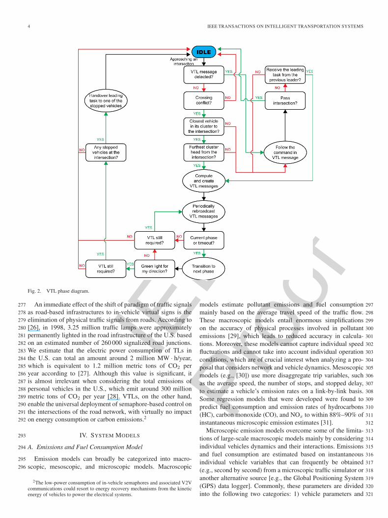
whenever necessary. Fig. 2 depicts the principle of the operation 258
of the VTL system in terms of stages. 259
In a primal paper, where the VTL concept was presented, the 260
dynamic performance of the system has also been studied. The 261
selected mobility metric was the average increase in flow rate 262
of the VTL protocol versus the real physical traffic signals as a 263
function of vehicle density. Large-scale simulations that emu- 264
late a real dense urban scenario provided compelling evidence 265
on the viability and significant benefits of the proposed scheme 266
in terms of the mobility metric (up to 60% increase at high 267
densities). This new self-organizing traffic paradigm thus holds 268
the potential for revolutionizing traffic control, particularly in 269
urban areas [6]. 270
The interaction between vehicles and pedestrians also needs 271
to be considered. The most direct and traditional approach that 272
could be foreseen is the communication of the traffic signal 273
information to pedestrians through smart phones or simple road 274
infrastructure. The virtual indication of traffic signals by the 275
leading vehicle is also proposed. 276
IEEE
Proo
f
4 IEEE TRANSACTIONS ON INTELLIGENT TRANSPORTATION SYSTEMS
Fig. 2. VTL phase diagram.
An immediate effect of the shift of paradigm of traffic signals277
as road-based infrastructures to in-vehicle virtual signs is the278
elimination of physical traffic signals from roads. According to279
[26], in 1998, 3.25 million traffic lamps were approximately280
permanently lighted in the road infrastructure of the U.S. based281
on an estimated number of 260 000 signalized road junctions.282
We estimate that the electric power consumption of TLs in283
the U.S. can total an amount around 2 million MW · h/year,284
which is equivalent to 1.2 million metric tons of CO2 per285
year according to [27]. Although this value is significant, it286
is almost irrelevant when considering the total emissions of287
personal vehicles in the U.S., which emit around 300 million288
metric tons of CO2 per year [28]. VTLs, on the other hand,289
enable the universal deployment of semaphore-based control on290
the intersections of the road network, with virtually no impact291
on energy consumption or carbon emissions.2292
IV. SYSTEM MODELS293
A. Emissions and Fuel Consumption Model294
Emission models can broadly be categorized into macro-295
scopic, mesoscopic, and microscopic models. Macroscopic296
2The low-power consumption of in-vehicle semaphores and associated V2Vcommunications could resort to energy recovery mechanisms from the kineticenergy of vehicles to power the electrical systems.
models estimate pollutant emissions and fuel consumption 297
mainly based on the average travel speed of the traffic flow. 298
These macroscopic models entail enormous simplifications 299
on the accuracy of physical processes involved in pollutant 300
emissions [29], which leads to reduced accuracy in calcula- 301
tions. Moreover, these models cannot capture individual speed 302
fluctuations and cannot take into account individual operation 303
conditions, which are of crucial interest when analyzing a pro- 304
posal that considers network and vehicle dynamics. Mesoscopic 305
models (e.g., [30]) use more disaggregate trip variables, such 306
as the average speed, the number of stops, and stopped delay, 307
to estimate a vehicle’s emission rates on a link-by-link basis. 308
Some regression models that were developed were found to 309
predict fuel consumption and emission rates of hydrocarbons 310
(HC), carbon monoxide (CO), and NOx to within 88%–90% of 311
instantaneous microscopic emission estimates [31]. 312
Microscopic emission models overcome some of the limita- 313
tions of large-scale macroscopic models mainly by considering 314
individual vehicles dynamics and their interactions. Emissions 315
and fuel consumption are estimated based on instantaneous 316
individual vehicle variables that can frequently be obtained 317
(e.g., second by second) from a microscopic traffic simulator or 318
another alternative source [e.g., the Global Positioning System 319
(GPS) data logger]. Commonly, these parameters are divided 320
into the following two categories: 1) vehicle parameters and 321

IEEE
Proo
f
FERREIRA AND D’OREY: IMPACT OF VIRTUAL TRAFFIC LIGHTS ON CARBON EMISSIONS MITIGATION 5
2) traffic/road parameters. Vehicle parameters include, among322
others, vehicle mass, fuel type, engine displacement, and ve-323
hicle class. On the other hand, network parameters (traffic and324
road conditions) account for instantaneous vehicle kinematics325
(e.g., speed or acceleration), aggregated variables (e.g., the326
time spent in the acceleration mode), or road characteristics327
(e.g., road grade). Because microscopic emission and fuel328
consumption models have higher temporal precision and better329
capture the effects of vehicle dynamics/interactions, they are330
better suited to evaluate the environmental gains derived from331
an ITS measure, such as the VTL system.332
Several microscopic models have been proposed by the333
scientific community. These models can be classified into334
emission maps (speed/acceleration lookup tables), purely sta-335
tistical models, and load-based models [32]. Major contribu-336
tions in this field were given by Akcelik et al. [33], Barth337
et al. [34] with the comprehensive modal emission model338
(CMEM), Ahn et al. [35], and Cappiello et al. [32] with339
the emissions from traffic (EMIT) model. The latter model340
has been selected due to computational performance and ac-341
curacy reasons. EMIT is a simple dynamic emission model342
that was derived from statistical and load-based emission343
models.344
This model first estimates the instantaneous tractive power345
(Ptr) using (1), which has the vehicle velocity v (in meters per346
second) and acceleration a (in square meters per second) as the347
main parameters348
Ptr =A · v+B · v2+C · v3+M · a · v+M · g · sinϑ · v (1)
where the variables are defined as follows:349
A rolling resistance (in kilowatts per meter per second);350
B speed correction (in kilowatts per square meter per351
second);352
C air drag resistance (in kilowatts per cubic meter per353
second);354
M vehicle mass (in kilograms);355
g gravitational constant (in square meters per second);356
ϑ road grade (in degrees).357
Depending on the value of Ptr, the fuel rate (FR) can be358
expressed as359
FR ={
αi + βiv + γiv2 + δiv
3 + ζiav, if Ptr > 0α′
i, if Ptr = 0(2)
where αi, βi, γi, δi, and ζi are constants that are associated360
with individual vehicles that were obtained using ordinary least361
square linear regressions.362
The EMIT model allows us to simultaneously calculate363
several pollutant emissions subproducts, i.e., CO, CO2, HC,364
and nitrogen oxide (NO). This calculation is divided into the365
following two main phases: 1) engine-out (EO) and 2) tailpipe366
(TP). The following formula for calculating EO pollutant emis-367
sions has the same structure as (2) due to the linear relationship368
with FR:369
EOi = α + µ · FR (3)
Fig. 3. CO2 emissions surface as a function of the vehicle acceleration andvelocity; increasing values for this metric lead to increased CO2 emissions.The EMIT model can produce negative values.
CO2 is the main by-product of the combustion of fossil 370
fuels,3 and consequently, it is proportional to the FR. The 371
values of CO2 EO emissions are directly estimated from fuel 372
consumption estimates. Due to this linear relationship, the 373
terms FR or CO2 can interchangeably be used when analyzing 374
the environmental impact of an ITS technology. Fig. 3 depicts 375
the CO2 emissions surface for a given input parameter set 376
(acceleration and velocity) with a resolution of 0.1 (m/s2 and 377
m/s, respectively). Note that negative values for CO2 can be 378
obtained with the EMIT model. This problem was addressed 379
by considering a minimum value for the emissions that is equal 380
to the constant α′i when Ptract is equal to zero. 381
After estimating the EO emission for the subproducts of 382
combustion, the EMIT model calculates the TP emission rates. 383
This emission rate is a fraction of the EO emission rate that 384
leaves the catalytic converter, i.e., 385
TPi = EOi · CPFi (4)
where CPFi denotes the catalyst pass fraction for species i. 386
The calibration of the parameters of (1) and (2) resorted to 387
light-duty vehicle data that were gathered for CMEM. Because 388
our goal is to evaluate the relative benefit of the VTL technol- 389
ogy, we consider the same coefficients for all vehicles that are 390
used in this paper. These parameters are shown in Table I and 391
are based on the values available from the EMIT model [32] 392
(vehicle category 9).4 393
B. Microscopic Traffic Model 394
To test the feasibility and performance of VANET-based 395
applications, a simulation platform is required to simulate ve- 396
hicular ad hoc environments. The simulation-based evaluation 397
3Although, in this paper, we mainly assess CO2 emissions, which is the mainby-product of fossil fuels combustion, other subproducts could be evaluated dueto their relative importance, particularly at intersections due to the stop-and-gophenomenon.
4The definition of each vehicle/technology category of the modal emissionsmodel can be found in [36]. Vehicle category 9 represents a normal emittingcar (Tier 1 emission standard), with accumulated mileage greater than 50 000miles and high power/weight ratio.

IEEE
Proo
f
6 IEEE TRANSACTIONS ON INTELLIGENT TRANSPORTATION SYSTEMS
TABLE IEMIT MODEL PARAMETERS
of VANET protocols requires a network simulator (NS-3) and398
a road traffic microscopic simulator [Development of Interve-399
hicular Reliable Telematics (DIVERT)]. DIVERT [37], [38] is400
a sophisticated microscopic simulator based on the intelligent401
driver model (IDM) [39] with a validated mobility model402
[40]. The lane-changing model is based on the MOBIL modelAQ1 403
proposed by Treiber et al. in [41]. The mobility patterns are404
individually influenced by random initialization, within typical405
values, of attributes such as acceleration, braking, aggressive-406
ness, and risk tolerance [37]. The current mobility model does407
not account for vehicle speed adaptation based on the received408
information (e.g., driver reaction to traffic signal controller409
timing information) as done in [42]. The implementation in-410
cludes all the common features of a road transportation network411
(e.g., traffic signals). It allows the simulation of thousands412
of vehicles with a high degree of realism [38] and with a413
wide range of configurations (e.g., aggressiveness). NS-3 is a414
discrete-event network simulator for Internet systems, primar-415
ily targeting research and educational use [43]. Several radio416
access technologies (e.g., IEEE 802.11p), as well as multiple417
interfaces/channels features and various protocol modules, can418
be used. In [44], the authors conclude that NS-3 delivers the419
best overall performance.420
The need for a bidirectional coupling of these two com-421
ponents (network and traffic) is fundamental and has been422
discussed in [45]. Clearly, the mobility of vehicles affects the423
network connectivity and behavior. Conversely, the results of424
the network simulation component can also affect the mobility425
of vehicles. In the case of VTL, this bidirectional coupling is426
particularly microscopic in both directions. Detailed mobility427
information (e.g., the position, speed, and heading of each428
vehicle) needs to be fed to NS-3, which has been coupled429
with DIVERT [38] to simulate the beaconing, leader election,430
and virtual light messages in the context of the VTL protocol.431
Traffic signal information, which results from the exchange of432
messages of the VTL protocol emulated by NS-3, is provided to433
the DIVERT simulator; the individual mobility of each vehicle434
is affected by the regulatory messages conveyed by the VTL435
(e.g., stop at a given intersection).436
V. METHODOLOGY437
Our goal is to quantify the impact of the VTL technology438
on CO2 emissions mitigation. We should thus analyze CO2439
emissions of vehicles that interact with physical traffic signals 440
and compare the results with the CO2 emissions of vehicles 441
that use VTLs. To isolate the benefit of the VTL approach, 442
each of the alternatives for intersection control should have 443
identical settings in all possible static variables, including the 444
characteristics of vehicles and drivers, the road scenario, and 445
the routes. The differences in the two analyses result from a 446
different mobility behavior of each vehicle that is affected by 447
dynamic aspects, which correspond to different traffic condi- 448
tions due to alternative schemes of intersection control. 449
To perform these two analyses, the aforementioned EMIT 450
emissions model was integrated into a microscopic traffic sim- 451
ulator. The microscopic traffic simulator outputs the mobility 452
behavior of each vehicle in the form of a virtual GPS trace. 453
By processing this GPS trace, a set of variables can be derived, 454
such as acceleration and speed, which then feed the microscopic 455
emissions model. The emissions of each vehicle are then aggre- 456
gated to quantify the overall positive impact of the VTL system. 457
Fig. 4 illustrates this architecture and its main components. 458
The main component of the simulation-based evaluation of the 459
decarbonization impact of VTLs is the DIVERT microscopic 460
traffic simulator [37]. 461
The implementation of physical TLs and VTLs in DIVERT is 462
relatively simple and leverages on the car-following equations 463
included in the IDM [39] that affect the acceleration and decel- 464
eration patterns of each vehicle. In terms of mobility simulation, 465
physical and virtual traffic signals are identically implemented 466
in DIVERT. For each lane of an approach to an intersection, 467
the traffic simulator creates a temporary dimensionless vehicle 468
on the stop line associated with the lane. This dimensionless 469
vehicle is created under a red light and disappears under a 470
green or yellow light. Variable aggressiveness parameters of 471
each driver result in different behaviors under yellow lights 472
as a function of the distance to the stop line. The intermittent 473
creation of this dimensionless vehicle is thus mandated by 474
the traffic signal control system or the VTL protocol (see 475
Fig. 4) and transparently affects the mobility of vehicles based 476
on the car-following model that governs the acceleration and 477
deceleration variables. 478
The differences in the two instances of DIVERT illustrated 479
in Fig. 4 refer to the geographic location of physical TLs and 480
VTLs and to the method used to derive the TL color shown to 481
each vehicle. With regard to the geographic location of physical 482
traffic signals, we have replicated the existing deployment in the 483
city of Porto, Portugal. The implemented physical-TL approach 484
is also a loyal representation of the existing scenario. In the 485
current version of DIVERT, the traffic signal control system 486
is very simple and uses fixed green splits for each of the 487
approaches of an intersection. Such simplistic functioning is, 488
however, a good approximation of the current functioning of 489
most of the deployed traffic signals. A recent study has reported 490
that 70%–90% of the deployed traffic signals work under fixed 491
parameterization of cycle duration and green splits [46]. 492
The geographic location of VTL is not fixed and is de- 493
termined by traffic conditions in confluent approaches of an 494
intersection. Depending on the traffic density, such virtual 495
traffic signals can be present at all intersections or can be 496
almost nonexistent. Instead of the data from fixed traffic 497

IEEE
Proo
f
FERREIRA AND D’OREY: IMPACT OF VIRTUAL TRAFFIC LIGHTS ON CARBON EMISSIONS MITIGATION 7
Fig. 4. Evaluation architecture. The main component is the DIVERT microscopic traffic simulator, whose two instances are used to produce virtual GPS traces.The scenario road map, data on vehicles and drivers, and the route of each vehicle are fed to an instance of DIVERT with physical traffic signals and to anotherinstance where the VTL protocol is simulated. The simulation of the network layer of the VTL protocol is done by NS-3. The virtual GPS traces are then fed totwo instances of the EMIT model to compute and compare the aggregated values of CO2 emissions.
counters, the optimization of cycle duration and green splits of498
a VTL resorts to more complete information, which includes499
the position, speed, and heading of all vehicles that approach500
the intersection. This information is provided by DIVERT, and501
the simulation of its beaconing by each vehicle is done by NS-3.502
Leader election and the virtual light messages that are broadcast503
by the leader are also simulated in NS-3 and provide the traffic504
signal colors that are shown to each vehicle in DIVERT.5505
VI. RESULTS AND DISCUSSION506
The results and analysis presented here are based on the507
system models given in Section IV and follow the methodology508
provided in Section V (see also the framework depicted in509
Fig. 4). The two strategies (physical TL and VTL) are compared510
with making use of the simulation platform in a large-scale511
scenario (see Section VI-A) and a number of performance met-512
rics (see Section VI-B). First, individual vehicle dynamics are513
studied (see Section VI-C). To determine the overall benefit that514
arises from the implementation of the VTL system, individual515
outputs are consolidated (see Section VI-D).516
A. Simulation Scenario517
To give scale to the analysis of the benefits of VTLs, we518
evaluate the carbon emissions of vehicles in the road scenario519
of an entire city. The city of Porto, Portugal, which is the520
second largest in the country, spans an area of 41.3 km2 and521
has a road network that comprises 965 km. Due to a recent522
5Videos that show the principle of operation of the VTL system are avail-able at http://www.dcc.fc.up.pt/hc/vtl_porto.avi} and http://www.dcc.fc.up.pt/hc/vtl_complex.avi.
stereoscopic aerial survey over the city, where the location of all 523
moving vehicles was pinpointed and their traveling speeds were 524
derived, together with the inference of a 5-s route [40], realistic 525
traffic data are available for Porto. In the aerial survey, a total 526
of 10 566 vehicles were pinpointed. The observed distribution 527
of vehicles per road segment was used to (decrease) increase 528
density to (non)rush-hour values to evaluate the impact of VTL 529
under different conditions. In this paper, the following four 530
different densities of vehicles that move in the city of Porto are 531
then considered: 532
1) 24 veh/km2 (low); 533
2) 120 veh/km2 (medium-low); 534
3) 251 veh/km2 (medium-high); 535
4) 333 veh/km2 (high). 536
With regard to the route of each vehicle, random origin/ 537
destination pairs that are based on the observed distribution 538
of vehicles from the aerial survey are generated. We evaluate 539
mobility propagation using wireless transmission ranges of 540
150–250 m, as defined in [40]. In this paper, stereoscopic aerial 541
photography was used to model urban mobility to compute con- 542
nectivity and path availability. Communication is mostly direct 543
(one-hop communication) between the leader and vehicles in 544
the vicinity of an intersection. 545
The road network of the city of Porto has a total of 1991 546
intersections. Physical TLs control 328 of these 1991 intersec- 547
tions (16%). Fig. 5 depicts the road network, the location of 548
signalized intersections, and one example route followed by a 549
vehicle.6 Each scenario was evaluated for a period of 30 min. 550
6A zoomable webmap that shows the road network, the location of signalizedintersections, and the position of vehicles from the aerial survey is available athttp://drive-in.cmuportugal.org/porto/.

IEEE
Proo
f
8 IEEE TRANSACTIONS ON INTELLIGENT TRANSPORTATION SYSTEMS
Fig. 5. Road network of the city of Porto comprises 965 km of extension. The red dots display the location of the 328 intersections that are managed by physicaltraffic signals. The blue line represents an example of a route traversed by a vehicle in this paper.
B. Performance Metrics551
To demonstrate the benefits of the VTL system, a number of552
variables need to be analyzed. In [6], the impact on the traffic553
flow of VTL was evaluated for the same scenario of the city554
of Porto. Results have shown an increase of up to 60% in flow555
rate for high-density scenarios. Here, we want to analyze the556
environmental impact of VTL, comparing the individual and557
aggregated CO2 emissions of vehicles that travel the exact same558
number of kilometers on the exact same roads, with and without559
the VTL system.560
For this analysis, the definition of each variable, application561
domain, whether for individual vehicle analysis or aggregated562
investigations, and unit is given as follows:563
• Instantaneous CO2 emissions EiCO2
(individual; in grams564
per second): Calculated for vehicle i using (2) after know-565
ing the outcome of (1) with appropriate coefficients (see566
Table I);567
• Route CO2 emissions (individual; in grams): cumulative568
sum of an individual vehicle CO2 emissions for its com-569
plete route;570
• Average CO2 emissions per vehicle (aggregated; in571
grams): defined as572
∑endt=0
∑ncars
i EiCO2
ncars(5)
where t iterates over the seconds of the simulation, and i573
iterates over all the individual cars.574
C. Individual Vehicle Results575
Before analyzing the aggregated results of CO2 emissions576
for all vehicles in the city of Porto scenario, we analyze the577
relevant variables for an individual vehicle, highlighting impor-578
tant differences between a route traversed with the VTL system579
and with the deployed physical-TL system. This preliminary 580
analysis using a single vehicle gives some intuition about the 581
understanding of the aggregated results. 582
The vehicle that was selected for the current analysis tra- 583
versed the city following a route (see Fig. 5) that combines 584
a major arterial road and a dense urban area with permanent 585
intersection conflicts, which clearly have distinct characteristics 586
and can lead to different performance. In this paper, medium 587
traffic density is considered (190 vehicles/km2). Although this 588
overall density is the same with TL and VTL, the distribution of 589
vehicles can be very different as a result from the distinct traffic 590
control schemes. 591
Fig. 6 depicts the main variables (velocity, acceleration, 592
instantaneous CO2 emissions, and route CO2 emissions) for 593
TL (in blue continuous lines) and VTL (in red dashed lines). 594
The variables velocity and acceleration were obtained from 595
the virtual GPS logger. Observing these variables, it is evident 596
that, without the VTL system, the car remained stopped for 597
longer periods mainly due to the semaphored intersections and 598
increased congestion. This fact is particularly evident when the 599
vehicle enters the city center area, which contains a higher 600
density of physical traffic signals and of vehicles. The ubiquity 601
of the VTL solution also led to faster intersection conflict 602
resolution and contributed to congestion dissipation. Another 603
interesting fact is that, with the TL system, the car takes ap- 604
proximately more than 25% of the time to travel the same route 605
for this traffic density. Stated otherwise, the average velocity 606
of the vehicle with the VTL system is considerably increased 607
compared with the physical-TL system. 608
Observing the graphic of the instantaneous CO2 emissions 609
depicted in Fig. 6, the correlation between this output and the 610
velocity/acceleration metrics is evident. Increasing accelera- 611
tion/velocity values leads to increasing instantaneous pollutant 612
emissions. On the other hand, a stopped vehicle has a constant 613
emission rate. The instantaneous emissions cannot directly be 614

IEEE
Proo
f
FERREIRA AND D’OREY: IMPACT OF VIRTUAL TRAFFIC LIGHTS ON CARBON EMISSIONS MITIGATION 9
Fig. 6. Individual vehicle metrics comparison [velocity, acceleration, instantaneous CO2 emissions, and cumulative CO2 emissions for the traversed route(medium vehicle density)]. The same vehicle traverses the exact same route with and without the VTL system. Differences in all metrics are evident. In addition,note that this particular vehicle takes less than half the time to complete its route with the VTL system.
compared between physical TLs and VTLs, because they hap-615
pen at different locations of the route. The relevant comparison616
is the cumulative route CO2 emissions, which highlights the im-617
pact of the implementation of the VTL. Observing this metric,618
it is clear that the overall number of stops during the route, as619
illustrated by the vehicle’s acceleration and deceleration levels,620
has a significant impact on vehicle emission rates [47]. For the621
example route, the cumulative fuel consumption is reduced by622
approximately 25%, mainly due to the increased traffic flow623
and consequent less transportation congestion, as well as the624
ubiquity of the VTL solution, which can detect the existence or625
not of intersection conflicts.626
D. Aggregated Results627
Apart from investigating the benefits for individual vehicles,628
the performance of the VTL system was evaluated by consider-629
ing all the vehicular interactions that take place in the complete630
transportation network. To perform this study, the individual631
pollutant emissions values are aggregated for each simulation to632
determine the metric average CO2 emissions per vehicle. This633
metric is widely used to determine the environmental impact of634
ITS. Furthermore, it is a referenced measure, which allows di-635
rection comparison of results in scenarios with different traffic636
flows.637
To make statistical inference, a number of observations of638
the system (eight simulation runs for each traffic density)639
were performed, followed by a statistical analysis to obtain640
an estimate of the selected performance metric. The mean of641
the metric average CO2 emissions per vehicle is the estimated642
parameter, and 95% confidence intervals for the estimator are643
considered in this paper.644
Fig. 7. Aggregated vehicle metric for TL and VTL comparison, given dif-ferent vehicle densities. This graphic highlights the increased impact of VTLas traffic density becomes higher. Confidence intervals are depicted for eachvehicle density and traffic control strategy (TL or VTL).
Fig. 7 represents the selected metric in the TL and VTL 645
scenarios and considers vehicles densities that range from low 646
density to high density. In both scenarios, with the increase 647
of the vehicle density, the average CO2 emissions per vehicle 648
increase. As the density increases, intersection conflicts become 649
more frequent, which causes increased congestion. Increased 650
congestion leads to the stop-and-go phenomenon, which is 651
associated with constant accelerations and decelerations that 652
are one of the main causes of pollutant emissions. For all 653
vehicle densities, the average CO2 emissions per vehicle are 654
lower for the VTL case. 655

IEEE
Proo
f
10 IEEE TRANSACTIONS ON INTELLIGENT TRANSPORTATION SYSTEMS
Fig. 8. Improvement in terms of CO2 emissions due to the implementation ofthe VTL system in function of the vehicle density.
Fig. 8 depicts the percentage of improvement in terms of CO2656
emissions as a function of the vehicle density. The implementa-657
tion of the VTL system is beneficial in terms of CO2 emissions658
for all the traffic densities that were studied. In addition, as the659
car density increases, the mitigation in terms of CO2 becomes660
more evident. For the selected vehicle densities, the benefit661
varies between 1% and 18%. Eventually, if we increase the662
densities to higher values (which are unrealistic for the capacity663
of the current traffic control system of the city), the benefit664
would start declining, as the theoretical capacity of the road665
network, independent of the intersection control scheme that is666
used, starts to be reached.667
Note that there is also a significant increase on the average668
vehicle velocity between 26% (low density) and 41% (high669
density). In urban scenarios, however, this case does not lead670
to increased emissions, because the optimal cruising speed is671
never reached. The mitigation of carbon emissions occurs due672
to self-organized ubiquitous traffic control enabled by VTL.673
At high vehicle densities, the absence of traffic signals at674
intersections exacerbates the congestion problem, which leads675
to increased emissions in the physical-TL case. The results676
presented herein are in accordance with the results published677
in [6], where the vehicle traffic flow was studied.678
VII. CONCLUSION679
The advent of wireless intervehicle communication, which680
should be available in the near future, opens a variety of681
opportunities to increase the safety and efficiency of road682
utilization. With regard to efficiency, an important aspect of its683
optimization will involve the mitigation of pollutants emission684
to fight global warming and climate change. In this paper,685
we have addressed the evaluation of the environmental impact686
of a challenging application of intervehicle communication,687
called VTL. Such a system will have to overcome complex688
problems that are intrinsic to the critical control of the right of689
way of vehicles in an intersection through a distributed system690
based on wireless communications. In particular, VTLs face the691
hurdle of requiring 100% deployment in motorized vehicles to 692
work. However, this penetration problem is a common issue 693
for a variety of other V2V or V2I applications; safety-related 694
applications are a main example that requires high penetration 695
rates for effectiveness and are pushed forward for their evident 696
advantages. Reaching this level of deployment requires govern- 697
mental commitment to mandate the existing motorized vehi- 698
cles to install VTLs as an after-market equipment.7 To tackle 699
this issue, studies must be performed to investigate whether 700
changes can be made to the original VTL system to allow 701
lower penetration rates and the coexistence with the current TL 702
system. 703
In addition to the significant improvements in traffic flow 704
that have been reported in the work of Ferreira et al. and AQ2705
to the increased safety of semaphore-controlled intersections, 706
where accidents can be reduced by more than 30%, this paper 707
has reported a reduction of 18% for the CO2 emissions of a 708
realistic number of vehicles that travel in a large-scale urban 709
scenario when using the VTL system. Considering only the 710
CO2 component of the annual circulation tax that is in place 711
in Germany, for example, 2C/g/km, would justify the cost of 712
an after-market VTL system for any car owner. 713
This paper has been performed for internal combustion- 714
engine vehicles. As further work, we plan to investigate the 715
energy savings that arise from the implementations of ITS 716
measures for hybrid or electric vehicles, which currently have 717
limited autonomy. Furthermore, the simulator should be ex- 718
tended to include alternative emissions-modeling approaches 719
and also modified to perform the calculation in real time of 720
the energy/fuel consumption rather than postprocessing the in- 721
formation. This approach would allow testing innovative algo- 722
rithms where parameters are changed online, depending on the 723
current energy consumption or emissions. Another interesting 724
topic to study in more detail is pedestrian–vehicle interaction 725
and human–computer interaction. 726
The inclusion of urban traffic control (UTC) systems in 727
simulation can provide additional insights into the intersection 728
control problem. More specifically, the benefit of the VTL 729
approach compared to such centralized control systems will 730
be studied. In the city of Porto, such UTC systems have been 731
deployed to control part of the traffic signals. We are currently 732
integrating in our simulation platform a replication of the func- 733
tioning of this UTC based on simulated inputs that correspond 734
to activations of virtual inductive-loop sensors. This line of 735
research involves joint work with the company that develops 736
the UTC system to have a virtual replication of the system that 737
mimics the exact behavior of the traffic signals that are in place 738
in the city of Porto. 739
ACKNOWLEDGMENT 740
The authors would like to thank the anonymous reviewers for 741
their valuable and detailed comments and suggestions, which 742
helped improve the quality of this paper. 743
7Electronic tolling systems and in-vehicle parking meters are examples ofsystems that have been the subject of legislation in some parts of the world.

IEEE
Proo
f
FERREIRA AND D’OREY: IMPACT OF VIRTUAL TRAFFIC LIGHTS ON CARBON EMISSIONS MITIGATION 11
REFERENCES744
[1] “Towards a resource-efficient transport system,” Eur. Environment745Agency, Copenhagen, Denmark, EEA Rep. 2/2010, 2010.746
[2] T. Nadeem, S. Dashtinezhad, C. Liao, and L. Iftode, “TrafficView: Traf-747fic data dissemination using car-to-car communication,” in SIGMOBILE748Mob. Comput. Commun. Rev., Jul. 2004, vol. 8, no. 3, pp. 6–19.749
[3] T. Yamashita, K. Izumi, and K. Kurumatani, “Car navigation750with route information sharing for improvement of traffic efficiency,”751in Proc. IEEE Int. Conf. Intell. Transp. Syst., Washington, DC, 2004,752pp. 465–470.753
[4] T. Tank and J. Linnartz, “Vehicle-to-vehicle communications for AVCS754platooning,” IEEE Trans. Veh. Technol., vol. 46, no. 2, pp. 528–536,755Mar. 1997.756
[5] V. Gradinescu, C. Gorgorin, R. Diaconescu, V. Cristea, and L. Iftode,757“Adaptive traffic lights using car-to-car communication,” in Proc. IEEE758Veh. Technol. Conf., Dublin, Ireland, Apr. 2007, pp. 21–25.759
[6] M. Ferreira, R. Fernandes, H. Conceição, W. Viriyasitavat, and760O. K. Tonguz, “Self-organized traffic control,” in Proc. ACM Int. Work-761shop Veh. InterNETwork., Chicago, IL, 2010, pp. 85–90.762
[7] S. Lämmer and D. Helbing, “Self-stabilizing decentralized signal control763of realistic, saturated network traffic,” Santa Fe Institute, Santa Fe, NM,764Tech. Rep. 10-09-019, 2010.765
[8] G. Zhang and Y. Wang, “Optimizing minimum and maximum green766time settings for traffic actuated control at isolated intersections,”767IEEE Trans. Intell. Transp. Syst., vol. 12, no. 1, pp. 164–173,768Mar. 2011.769
[9] J. Barnes, V. Paruchuri, and S. Chellappan, “On optimizing traffic signal770phase ordering in road networks,” in Proc. IEEE Symp. Reliab. Distrib.771Syst., New Delhi, India, Nov. 2010, pp. 308–312.772
[10] P. Hunt, D. Robertson, R. Bretherton, and M. Royle, “The SCOOT online773traffic signal optimisation technique,” Traffic Eng. Control, vol. 23, no. 4,774pp. 190–192, Apr. 1982.775
[11] P. Lowrie, “The Sydney coordinated adaptive traffic system—Principles,776methodology, algortithms,” in Proc. IEE Int. Conf. Road Traffic Signall.,7771982, pp. 35–41.778
[12] T. Tielert, M. Killat, H. Hartenstein, R. Luz, S. Hausberger, and779T. Benz, “The impact of traffic-light-to-vehicle communication on fuel780consumption and emissions,” in Proc. Internet Things Conf., Tokyo,781Japan, Nov. 2010, pp. 1–8.782
[13] C. Cai, Y. Wang, and G. Geers, “Adaptive traffic signal783control using vehicle-to-infrastructure communication: A technical784note,” in Proc. Int. Workshop Comput. Transp. Sci., San Jose, CA, 2010,785pp. 43–47.786
[14] B. Gokulan and D. Srinivasan, “Distributed geometric fuzzy multiagent787urban traffic signal control,” IEEE Trans. Intell. Transp. Syst., vol. 11,788no. 3, pp. 714–727, Sep. 2010.789
[15] E. W. Martin and S. A. Shaheen, “Greenhouse gas emission impacts ofAQ3 790carsharing in North America,” IEEE Trans. Intell. Transp. Syst., to be791published.792
[16] M. Bell, “Environmental factors in intelligent transport systems,” in Proc.793IEE Intell. Transp. Syst., Jun. 2006, vol. 153, no. 2, pp. 113–128.794
[17] H. Liimatainen, “Utilization of fuel consumption data in an ecodrivingAQ4 795incentive system for heavy-duty vehicle drivers,” IEEE Trans. Intell.796Transp. Syst., to be published.797
[18] M. A. S. Kamal, M. Mukai, J. Murata, and T. Kawabe, “Ecological vehicle798control on roads with up-down slopes,” IEEE Trans. Intell. Transp. Syst.,799vol. 12, no. 3, pp. 783–794, Sep. 2011.800
[19] S. Tsugawa and S. Kato, “Energy ITS: Another application of vehicular801communications,” IEEE Commun. Mag., vol. 48, no. 11, pp. 120–126,802Nov. 2010.803
[20] C. Sommer, R. Krul, R. German, and F. Dressler, “Emissions804versus travel time: Simulative evaluation of the environmental impact805of ITS,” in Proc. IEEE Veh. Technol. Conf., Taipei, Taiwan, May 2010,806pp. 1–5.807
[21] R. D. Watts, R. W. Compton, J. H. McCammon, C. L. Rich,808S. M. Wright, T. Owens, and D. S. Ouren, “Roadless space of the809conterminous United States,” Science, vol. 316, no. 5825, pp. 736–738,810May 2007.811
[22] United States Census Bureau, The Tiger/Line Database. [Online]. Avail-812able: http://www.census.gov/geo/www/tiger/813
[23] J. E. Williams and J. D. Griffiths, “The geometrical design of signalised814road traffic junctions,” in Proc. Conf. Winter Simul., Atlanta, GA, 1987,815pp. 819–827.816
[24] D. Robertson and R. D. Bretherton, “Optimizing networks of traffic817signals in real time—The SCOOT method,” IEEE Trans. Veh. Technol.,818vol. 40, pt. 2, no. 1, pp. 11–15, Feb. 1991.819
[25] C. Maihofer, “A survey of geocast routing protocols,” IEEE 820Commun. Surveys Tuts., vol. 6, no. 2, pp. 32–42, Second Quarter, 8212009. 822
[26] M. Suozzo, “A market transformation opportunity assessment for LED 823traffic signals,” Amer. Council Energy-Efficient Economy, Washington, 824DC, Res. Rep. A983, 1998. 825
[27] “Carbon dioxide emissions from the generation of electric power in the 826United States,” Dept. Energy Environ. Protection Agency, Washington, 827DC, 2000. 828
[28] J. Decicco and F. Fung, “Global warming on the road—The climate 829impact of America’s automobiles,” Environmental Defense, Washington, 830DC, 2006. 831
[29] L. I. Panis, S. Broekx, and R. Liu, “Modeling instantaneous traffic emis- 832sion and the influence of traffic speed limits,” Sci. Total Environ., vol. 371, 833no. 1–3, pp. 270–285, Dec. 2006. 834
[30] H. Yue, “Mesoscopic fuel consumption and emission modeling,” Ph.D. 835dissertation, Virginia Polytechnic Inst. State Univ., Blacksburg, VA, 8362008. 837
[31] Y. Ding and H. Rakha, “Trip-based explanatory variables for estimating 838vehicle fuel consumption and emission rates,” Water Air Soil Pollution: 839Focus, vol. 2, no. 5/6, pp. 61–77, Sep. 2002. 840
[32] A. Cappiello, I. Chabini, E. Nam, A. Lue, and M. Abou Zeid, “A statistical 841model of vehicle emissions and fuel consumption,” in Proc. IEEE Int. 842Conf. Intell. Transp. Syst., Singapore, 2002, pp. 801–809. 843
[33] R. Akcelik and M. Besley, “Operating cost, fuel consumption and emis- 844sion models in aaSIDRA and aaMOTION,” in Proc. Conf. Australian Inst. 845Transp. Res., Dec. 2003, pp. 1–14. 846
[34] F. An, M. Barth, J. Norbeck, and M. Ross, “Development of com- 847prehensive modal emissions model: Operating under hot-stabilized 848conditions,” Transp. Res. Rec., vol. 1587, no. 1, pp. 52–62, 849Jan. 1997. 850
[35] K. Ahn, H. Rakha, A. Trani, and M. V. Aerde, “Estimating vehi- 851cle fuel consumption and emissions based on instantaneous speed and 852acceleration levels,” J. Transp. Eng., vol. 128, no. 2, pp. 182–190, 853Mar./Apr. 2002. 854
[36] M. Barth, F. An, T. Younglove, G. Scora, C. Levine, M. Ross, and 855T. Wenzel, “Development of a comprehensive modal emissions 856model,” Nat. Cooperative Highway Res. Program, Transp. Res. Board, 857Washington, DC, Tech. Rep., 2000. 858
[37] H. Conceição, L. Damas, M. Ferreira, and J. Barros, “Large-scale sim- 859ulation of V2V environments,” in Proc. ACM Symp. Appl. Comput., 860Fortaleza, Brazil, 2008, pp. 28–33. 861
[38] R. Fernandes, P. M. d’Orey, and M. Ferreira, “DIVERT for realistic simu- 862lation of heterogeneous vehicular networks,” in Proc. IEEE Int. Workshop 863Intell. Veh. Netw., San Francisco, CA, 2010, pp. 721–726. 864
[39] M. Treiber, A. Hennecke, and D. Helbing, “Congested traffic states in em- 865pirical observations and microscopic simulations,” Phys. Rev. E, vol. 62, 866no. 2, pp. 1805–1824, Aug. 2000. 867
[40] M. Ferreira, H. Conceição, R. Fernandes, and O. Tonguz, “Stereoscopic 868aerial photography: An alternative to model-based urban mobility ap- 869proaches,” in Proc. ACM Int. Workshop Veh. InterNETw., Beijing, China, 8702009, pp. 53–62. 871
[41] M. Treiber and A. Kesting, “An open-source microscopic traffic sim- 872ulator,” IEEE Intell. Transp. Syst. Mag., vol. 2, no. 3, pp. 6–13, 873Fall 2010. 874
[42] V. Milanes, J. Perez, E. Onieva, and C. Gonzalez, “Controller for ur- 875ban intersections based on wireless communications and fuzzy logic,” 876IEEE Trans. Intell. Transp. Syst., vol. 11, no. 1, pp. 243–248, 877Mar. 2010. 878
[43] The Network Simulator NS-3. [Online]. Available: http://www.nsnam. 879org/ 880
[44] E. Weingartner, H. vom Lehn, and K. Wehrle, “A performance compar- 881ison of recent network simulators,” in Proc. IEEE Int. Conf. Commun., 882Jun. 2009, pp. 1–5. 883
[45] C. Sommer, R. German, and F. Dressler, “Bidirectionally 884coupled network and road traffic simulation for improved IVC 885analysis,” IEEE Trans. Mobile Comput., vol. 10, no. 1, pp. 3–15, 886Jan. 2011. 887
[46] Transp. Res. Board, Adaptive Traffic Control Systems: 888Domestic and Foreign State of Practice, 2010, NCHRP 889Synthesis 403. 890
[47] H. Rakha and Y. Ding, “Impact of stops on vehicle fuel consump- 891tion and emissions,” J. Transp. Eng., vol. 129, no. 1, pp. 23–32, 892Jan./Feb. 2003. 893
[48] U.S. Department of Transportation-Institute of Transportation Engineers, 894“Toolbox of Countermeasures and Their Potential Effectiveness to Make 895Intersections Safer,” Briefing Sheet 8, 2004. 896

IEEE
Proo
f
12 IEEE TRANSACTIONS ON INTELLIGENT TRANSPORTATION SYSTEMS
Michel Ferreira received the B.S. and Ph.D. degrees897in computer science from the University of Porto,898Porto, Portugal, in 1994 and 2002, respectively.899
He is currently an Assistant Professor of computer900science with the Departmento de Ciência de Com-901putadores, Faculdade de Ciências, Universidade do902Porto, where he is also a Researcher with the Porto903Laboratory, Instituto de Telecomunicaçðes, and leads904the Geonetworks Group. In 2005, he held a visiting905position with the University of New Mexico, Albu-906querque, while he was on a sabbatical leave. His907
research interests include vehicular networks, spatiodeductive databases, and908computer simulation. He has led several research projects in logic-based spatial909databases, vehicular sensing, and intervehicle communication.910
Pedro M. d’Orey received the Licenciatura degree 911in electrical and computer engineering from the Uni- 912versidade do Porto, Porto, Portugal, in 2004 and 913the M.Sc. degree in telecommunications from the 914University of London, London, U.K., in 2008. He is 915currently working toward the Ph.D. degree with the 916Universidade do Porto. 917
He held several positions in the mobile commu- 918nications industry. He is currently a Researcher with 919the Instituto de Telecomunicaçðes, Departmento de 920Ciência de Computadores, Faculdade de Ciências, 921
Universidade do Porto. His research interests include intelligent transportation 922systems, vehicular networks, green computing, and self-optimization. 923

IEEE
Proo
f
AUTHOR QUERIES
AUTHOR PLEASE ANSWER ALL QUERIES
AQ1 = What does MOBIL stand for?AQ2 = Reference citations in the Conclusion are not allowed as per the Style Manual, so [6] was omitted.
Please check if wording is appropriate.AQ3 = Please provide publication update for Ref. [15].AQ4 = Please provide publication update for Ref. [17].
END OF ALL QUERIES

IEEE
Proo
f
IEEE TRANSACTIONS ON INTELLIGENT TRANSPORTATION SYSTEMS 1
On the Impact of Virtual Traffic Lightson Carbon Emissions Mitigation
1
2
Michel Ferreira and Pedro M. d’Orey3
Abstract—Considering that the transport sector is responsible4for an increasingly important share of current environmental5problems, we look at intelligent transportation systems (ITS) as6a feasible means of helping in solving this issue. In particular, we7evaluate the impact in terms of carbon dioxide (CO2) emissions of8virtual traffic light (VTL), which is a recently proposed infrastruc-9tureless traffic control system solely based on vehicle-to-vehicle10(V2V) communication. Our evaluation uses a real-city scenario11in a complex simulation framework, involving microscopic traffic,12wireless communication, and emission models. Compared with an13approximation of the physical traffic light system deployed in the14city, our results show a significant reduction on CO2 emissions15when using VTLs, reaching nearly 20% under high-density traffic.16
Index Terms—Carbon dioxide (CO2) emissions, fuel consump-17tion, vehicular ad hoc networks (VANETs), virtual traffic lights18(VTLs).19
I. INTRODUCTION20
G LOBAL warming and climate change have impacted the21
policy scene for the implementation of measures toward22
low-carbon resource-efficient economies. Decarbonization of23
the transport sector is particularly important, because in the24
European Union (EU), this sector accounts for around 25% of25
total carbon dioxide (CO2) emissions, according to a study of26
the European Environment Agency (EEA) [1]. This same study27
also reports that car journeys comprised 72% of all passenger28
kilometers in EU-27 (excluding Cyprus and Malta) and have29
clearly represented the dominant mode of transport over the30
past few decades. One aggravating factor is the ever-increasing31
traffic levels that have neutralized the average emissions reduc-32
tion per vehicle obtained due to the design of more efficient33
vehicles.34
In parallel with the effort to develop more efficient and35
environmentally friendly vehicles, the design of mechanisms36
that improve the efficiency of road utilization, i.e., real-time37
traffic information systems and collaborative routing systems38
Manuscript received October 8, 2010; revised March 1, 2011, July 4,2011, and August 31, 2011; accepted September 17, 2011. This work wassupported in part by the Information and Communication Technologies In-stitute: a joint institute between Carnegie Mellon University and Portugal,through the project “DRIVE-IN: Distributed Routing and Infotainment throughVehicular Internetworking” under Grant CMU-PT/NGN/0052/2008 and by thePortuguese Foundation for Science and Technology and NDrive under GrantSFRH/BD/71620/2010. The Associate Editor for this paper was M. Brackstone.
The authors are with the Instituto de Telecomunicaçðes, Departmentode Ciência de Computadores, Faculdade de Ciências, Universidade doPorto, 4169-007 Porto, Portugal (e-mail: [email protected]; [email protected]).
Color versions of one or more of the figures in this paper are available onlineat http://ieeexplore.ieee.org.
Digital Object Identifier 10.1109/TITS.2011.2169791
[2], [3], highway platooning [4], or adaptive traffic signal con- 39
trol [5], [6], can produce substantial additional benefits toward 40
the reduction of the carbon footprint of road transportation. 41
In the critical fraction of CO2 g/km, we argue that more 42
emphasis should be put on the mechanics of how each kilometer 43
is traveled, including the route choice and the traffic control 44
signage that is in place. In-vehicle intelligent transportation 45
system (ITS) technologies will play a key role in this more 46
efficient utilization of the road as we witness the inclusion of 47
routing engines and traffic signs as in-vehicle systems. 48
Aside from improving safety and road network efficiency, we 49
argue that ITS measures lead to significant improvements in 50
terms of environmental impact. Thus, evaluating and quantify- 51
ing the impact of such technologies in terms of CO2 emissions 52
is very important and can eventually lead to its integration 53
in the assignment of the emissions value of new cars, which 54
is relevantly reflected in the final price/yearly taxes and can 55
contribute to a more rapid dissemination of such technologies. 56
In this paper, we focus on the evaluation and quantification of 57
the impact in terms of CO2 emissions of the recently proposed 58
concept of virtual traffic lights (VTLs) [6], where the traditional 59
road-based physical traffic signals are replaced by in-vehicle 60
representations, supported only by vehicle-to-vehicle (V2V) 61
communication. Our main goal is to provide evidence of the 62
significant reductions in average network emissions that can be 63
obtained through a novel ITS technology enabled by vehicular 64
ad hoc networks (VANETs). Furthermore, we aim at providing 65
a methodology and an associated simulation platform to study 66
the environmental impact of any ITS measure. 67
The remainder of this paper is organized as follows. In 68
the next section, we briefly present the relevant related work 69
in traffic signal control and the environmental impact of ITS 70
measures. Then, Section III introduces the VTL concept and the 71
system main characteristics. Section IV provides an overview 72
on the main system models, i.e., emissions and fuel consump- 73
tion (see Section IV-A) and the microscopic traffic model (see 74
Section IV-B). Section V presents a methodology for evaluating 75
carbon emissions and the impact that the VTL system has on 76
their mitigation. Section VI details the simulation scenario and 77
evaluation metrics and provides the main results (individual 78
and aggregated). Section VII closes this paper with the main 79
conclusions. 80
II. RELATED WORK 81
A. Traffic Signal Control 82
Traffic signal control has attracted much attention from 83
the research community over the past few decades. Classical 84
1524-9050/$26.00 © 2011 IEEE
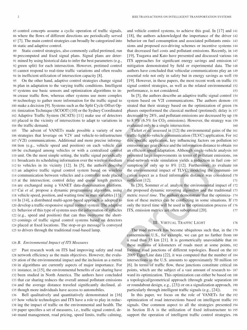
IEEE
Proo
f
2 IEEE TRANSACTIONS ON INTELLIGENT TRANSPORTATION SYSTEMS
control concepts assume a cyclic operation of traffic signals,85
where the flows of different directions are periodically served86
[7]. The main control strategies can broadly be categorized into87
static and adaptive control.88
Static control strategies, also commonly called pretimed, run89
precomputed and fixed signal plans. Signal plans are deter-90
mined by using historical data to infer the best parameters (e.g.,91
green split) for each intersection. However, pretimed control92
cannot respond to real-time traffic variations and often results93
in inefficient utilization of intersection capacity [8].94
On the other hand, adaptive control strategies change signal95
plan in adaptation to the varying traffic conditions. Intelligent96
systems use basic sensors and optimization algorithms to in-97
crease traffic flow, whereas other systems use more complex98
technology to gather more information for the traffic signal to99
make a decision [9]. Systems such as the Split Cycle Offset Op-100
timization Technique (SCOOT) [10] or the Sydney Coordinated101
Adaptive Traffic System (SCATS) [11] make use of detectors102
placed in the vicinity of intersections to adapt to variations in103
the traffic demand.104
The advent of VANETs made possible a variety of new105
strategies that leverage on V2V and vehicle-to-infrastructure106
(V2I) communications. Additional and more precise informa-107
tion (e.g., vehicle speed and position) on each vehicle can108
be exchanged among vehicles or with a centralized control109
unit. On the most simple setting, the traffic signal periodically110
broadcasts its scheduling information over the wireless medium111
to vehicles in its vicinity [12]. In [5], the authors describe112
an adaptive traffic signal control system based on wireless113
communication between vehicles and a controller node placed114
at the intersection; control delay and queue length metrics115
are exchanged using a VANET data-dissemination platform.116
Cai et al. propose a dynamic programming algorithm, using117
vehicle speed, position, and waiting time as state variables [13].118
In [14], a distributed multi-agent-based approach is adopted to119
develop a traffic-responsive signal control system. The adaptive120
behavior of this type of systems uses the information of vehicles121
(e.g., speed and position) that can thus overcome the short-122
comings of traffic signal control systems based on detectors123
placed at fixed locations. The stop-or-go message is conveyed124
to drivers through the traditional road-based lamp.125
B. Environmental Impact of ITS Measures126
Past research work on ITS had improving safety and road127
network efficiency as the main objectives. However, the evalu-128
ation of the environmental impact and the inclusion as a metric129
in algorithms are currently aspects of major importance. For130
instance, in [15], the environmental benefits of car sharing have131
been studied in North America. The authors have concluded132
that car sharing reduces the overall annual pollutant emissions133
and the average distance traveled significantly declined, al-134
though more individuals have access to automobiles.135
Bell qualitatively and quantitatively demonstrated in [16]136
how vehicle technologies and ITS have a role to play in reduc-137
ing the impact of traffic on the environmental and health. The138
paper specifies a set of measures, i.e., traffic signal control, de-139
mand management, road pricing, speed limits, traffic calming,140
and vehicle control systems, to achieve this goal. In [17] and 141
[18], the authors acknowledged the importance of the driver 142
behavior on fuel consumption and associated pollutants emis- 143
sions and proposed eco-driving schemes or incentive systems 144
that decreased fuel costs and pollutant emissions. Recently, in 145
[19], Tsugawa and Kato have presented and discussed various 146
ITS approaches for significant energy savings and emission 147
mitigation demonstrated by field or experimental data. The 148
authors have concluded that vehicular communications play an 149
essential role not only in safety but in energy savings as well 150
[19]. However, in these papers, the most recent work on traffic 151
signal control strategies, as well as the related environmental 152
performance, is not considered. 153
In [5], the authors describe an adaptive traffic signal control 154
system based on V2I communications. The authors demon- 155
strated that their strategy based on the optimization of green 156
phases outperformed the classical method (pretimed); delay is 157
decreased by 28%, and pollutant emissions are decreased by up 158
to 8.9% (6.5% for CO2 emissions). However, the strategy was 159
evaluated only to a single intersection. 160
Tielert et al. assessed in [12] the environmental gains of the 161
traffic-light-to-vehicle communication (TLVC) application. For 162
this specific application, key influencing factors on pollution 163
emissions are gear choice and the information distance to obtain 164
an efficient speed adaptation. Although single-vehicle analysis 165
presented large improvements in terms of pollutant emissions, 166
road-network-wide simulation yields a reduction in fuel con- 167
sumption of only up to 8% [12]. Furthermore, to evaluate 168
the environmental impact of TLVC, modeling the communi- 169
cation aspect as a fixed information distance was considered 170
sufficient [12]. 171
In [20], Sommer et al. analyze the environmental impact of 172
the proposed dynamic rerouting algorithm and the traditional 173
metric travel time. The authors demonstrate that the optimiza- 174
tion of these metrics can be conflicting in some situations. If 175
only the travel time will be used in the optimization process of 176
ITS, emission metrics are often suboptimal [20]. 177
III. VIRTUAL TRAFFIC LIGHT 178
The road network has become ubiquitous such that, in the 179
conterminous U.S., for example, we can get no farther from 180
a road than 35 km [21]. It is geometrically unavoidable that 181
these millions of kilometers of roads meet at some points, 182
forming road junctions of different topologies. Based on the 183
2009 Tiger/Line data [22], it was computed that the number of 184
intersections in the U.S. amounts to approximately 50 million 185
[6]. In terms of traffic flow, these junctions constitute critical 186
points, which are the subject of a vast amount of research to- 187
ward its optimization. This optimization can either be based on 188
a topological/geometrical approach (through grade separation 189
or roundabout design, e.g., [23]) or on a signalization approach, 190
particularly through intelligent traffic signals (e.g., [24]). 191
In this paper, we focus on the role of VANETs for the 192
optimization of road intersections based on intelligent traffic 193
signals. One common aspect to all the strategies presented 194
in Section II-A is the utilization of fixed infrastructure to 195
support the operation of intelligent traffic control strategies. 196

IEEE
Proo
f
FERREIRA AND D’OREY: IMPACT OF VIRTUAL TRAFFIC LIGHTS ON CARBON EMISSIONS MITIGATION 3
Fig. 1. (a) Conflict-free intersection. Vehicle A uses periodic beaconing toadvertise its position and heading as it approaches the intersection. No conflictsare detected, and it is not necessary to create a VTL. (b) Periodic beaconingof concurrent vehicles results in the detection of a crossing conflict and inthe need to create a VTL. One of the conflicting vehicles is elected as theintersection leader and will create and control the VTL. This leader stops atthe intersection and replaces a road-based traffic signal in a temporary controlof the intersection. (c) Leader is stopped at the intersection and optimizes thefunctioning of the VTL based on the number of vehicles in each approach andperiodically broadcasts VTL messages with the color of each approach/lane.(d) When the cycle ends and the green light is assigned to the leader ap-proach/lane, the current leader selects a new leader from the vehicles stoppedunder red lights. This new leader continues the cycle. If there are no stoppedvehicles under red lights, then the VTL ceases to exist.
Furthermore, many of these strategies assume the existence of197
a centralized control unit1 and cyclic operation. In this paper,198
we propose a new paradigm, called VTL, in which control199
is decentralized and self organized, operation is acyclic, and200
traffic signal information is individually and directly presented201
in each vehicle. In our system, vehicles behave as sensors in the202
road transportation network.203
In [6], we presented the VTL concept, advocating for a204
paradigm shift from traffic signals as road-based infrastructures205
to traffic signals as in-vehicle virtual signs supported only by206
V2V communication. The implementation of the VTL system207
results in improved traffic flow due to the optimized manage-208
ment of individual intersections, which is enabled not only by209
the neighborhood awareness of VANET protocols but due to210
the scalability of the solution as well, which renders signalized211
control of intersections truly ubiquitous. This ubiquity allows us212
to maximize the throughput of the complete road network rather213
than the reduced number of road junctions that are currently214
managed by physical traffic signals.215
The principle of operation of VTLs is relatively simple and216
is illustrated in Fig. 1. Each vehicle has a dedicated application217
unit (AU), which maintains an internal database with informa-218
1A decentralized signal control strategy has recently been proposed byLaemmer and Helbing in [7].
tion about intersections where a VTL can be created. When 219
approaching such intersections, the AU checks whether there 220
is a VTL running that must be obeyed or a VTL needs to 221
be created as a result of perceiving crossing conflicts between 222
approaching vehicles [see Fig. 1(a) and (b)]. 223
Beaconing and location tables, which are features of VANET 224
geographical routing protocols (for example, see [25]), are used 225
to determine whether a VTL needs to be created. Each node 226
maintains a location table that contains information about every 227
node in its vicinity, which is constantly updated through the 228
reception of new beacons. The periodicity of these beacons can 229
be increased as vehicles approach an intersection. 230
If a VTL needs to be created, then all vehicles that approach 231
the intersection must agree on the election of one of the vehicles 232
as the leader, which will be responsible for creating the VTL 233
and broadcasting the traffic signal messages [see Fig. 1(c)]. 234
This vehicle works as a temporary virtual infrastructure for 235
the intersection and takes the responsibility of controlling the 236
VTL. Once this leader has been elected, a VTL cycle for 237
the intersection control is initiated with a red light for the 238
leader approach/lane. This condition ensures that the leader 239
will remain in the intersection for the duration of a complete 240
cycle. Based on the number of vehicles in each approach, the 241
leader can set the traffic signal parameters, such as the phase 242
layout and the green splits assigned to each approach, in an 243
optimized manner. During the existence of a VTL leader, the 244
other vehicles act as passive nodes in the protocol, listening 245
to traffic signal messages and presenting these messages to the 246
driver through the in-vehicle displays. 247
During a complete VTL cycle, the leader commutes the 248
traffic light (TL) phase among the conflicting approaches/lanes. 249
When the green light is in the leader’s lane, the control of the 250
VTL system must be handed over to a new leader in a different 251
approach/lane. If there are vehicles that stopped under the red 252
light at the intersection, the current leader selects one of these 253
vehicles to become the new leader, which will maintain the 254
intersection control in a consistent sequence [see Fig. 1(d)]. If 255
there are no stopped vehicles under the red light, then a new 256
leader will be elected through the previously explained process 257
whenever necessary. Fig. 2 depicts the principle of the operation 258
of the VTL system in terms of stages. 259
In a primal paper, where the VTL concept was presented, the 260
dynamic performance of the system has also been studied. The 261
selected mobility metric was the average increase in flow rate 262
of the VTL protocol versus the real physical traffic signals as a 263
function of vehicle density. Large-scale simulations that emu- 264
late a real dense urban scenario provided compelling evidence 265
on the viability and significant benefits of the proposed scheme 266
in terms of the mobility metric (up to 60% increase at high 267
densities). This new self-organizing traffic paradigm thus holds 268
the potential for revolutionizing traffic control, particularly in 269
urban areas [6]. 270
The interaction between vehicles and pedestrians also needs 271
to be considered. The most direct and traditional approach that 272
could be foreseen is the communication of the traffic signal 273
information to pedestrians through smart phones or simple road 274
infrastructure. The virtual indication of traffic signals by the 275
leading vehicle is also proposed. 276

IEEE
Proo
f
4 IEEE TRANSACTIONS ON INTELLIGENT TRANSPORTATION SYSTEMS
Fig. 2. VTL phase diagram.
An immediate effect of the shift of paradigm of traffic signals277
as road-based infrastructures to in-vehicle virtual signs is the278
elimination of physical traffic signals from roads. According to279
[26], in 1998, 3.25 million traffic lamps were approximately280
permanently lighted in the road infrastructure of the U.S. based281
on an estimated number of 260 000 signalized road junctions.282
We estimate that the electric power consumption of TLs in283
the U.S. can total an amount around 2 million MW · h/year,284
which is equivalent to 1.2 million metric tons of CO2 per285
year according to [27]. Although this value is significant, it286
is almost irrelevant when considering the total emissions of287
personal vehicles in the U.S., which emit around 300 million288
metric tons of CO2 per year [28]. VTLs, on the other hand,289
enable the universal deployment of semaphore-based control on290
the intersections of the road network, with virtually no impact291
on energy consumption or carbon emissions.2292
IV. SYSTEM MODELS293
A. Emissions and Fuel Consumption Model294
Emission models can broadly be categorized into macro-295
scopic, mesoscopic, and microscopic models. Macroscopic296
2The low-power consumption of in-vehicle semaphores and associated V2Vcommunications could resort to energy recovery mechanisms from the kineticenergy of vehicles to power the electrical systems.
models estimate pollutant emissions and fuel consumption 297
mainly based on the average travel speed of the traffic flow. 298
These macroscopic models entail enormous simplifications 299
on the accuracy of physical processes involved in pollutant 300
emissions [29], which leads to reduced accuracy in calcula- 301
tions. Moreover, these models cannot capture individual speed 302
fluctuations and cannot take into account individual operation 303
conditions, which are of crucial interest when analyzing a pro- 304
posal that considers network and vehicle dynamics. Mesoscopic 305
models (e.g., [30]) use more disaggregate trip variables, such 306
as the average speed, the number of stops, and stopped delay, 307
to estimate a vehicle’s emission rates on a link-by-link basis. 308
Some regression models that were developed were found to 309
predict fuel consumption and emission rates of hydrocarbons 310
(HC), carbon monoxide (CO), and NOx to within 88%–90% of 311
instantaneous microscopic emission estimates [31]. 312
Microscopic emission models overcome some of the limita- 313
tions of large-scale macroscopic models mainly by considering 314
individual vehicles dynamics and their interactions. Emissions 315
and fuel consumption are estimated based on instantaneous 316
individual vehicle variables that can frequently be obtained 317
(e.g., second by second) from a microscopic traffic simulator or 318
another alternative source [e.g., the Global Positioning System 319
(GPS) data logger]. Commonly, these parameters are divided 320
into the following two categories: 1) vehicle parameters and 321

IEEE
Proo
f
FERREIRA AND D’OREY: IMPACT OF VIRTUAL TRAFFIC LIGHTS ON CARBON EMISSIONS MITIGATION 5
2) traffic/road parameters. Vehicle parameters include, among322
others, vehicle mass, fuel type, engine displacement, and ve-323
hicle class. On the other hand, network parameters (traffic and324
road conditions) account for instantaneous vehicle kinematics325
(e.g., speed or acceleration), aggregated variables (e.g., the326
time spent in the acceleration mode), or road characteristics327
(e.g., road grade). Because microscopic emission and fuel328
consumption models have higher temporal precision and better329
capture the effects of vehicle dynamics/interactions, they are330
better suited to evaluate the environmental gains derived from331
an ITS measure, such as the VTL system.332
Several microscopic models have been proposed by the333
scientific community. These models can be classified into334
emission maps (speed/acceleration lookup tables), purely sta-335
tistical models, and load-based models [32]. Major contribu-336
tions in this field were given by Akcelik et al. [33], Barth337
et al. [34] with the comprehensive modal emission model338
(CMEM), Ahn et al. [35], and Cappiello et al. [32] with339
the emissions from traffic (EMIT) model. The latter model340
has been selected due to computational performance and ac-341
curacy reasons. EMIT is a simple dynamic emission model342
that was derived from statistical and load-based emission343
models.344
This model first estimates the instantaneous tractive power345
(Ptr) using (1), which has the vehicle velocity v (in meters per346
second) and acceleration a (in square meters per second) as the347
main parameters348
Ptr =A · v+B · v2+C · v3+M · a · v+M · g · sinϑ · v (1)
where the variables are defined as follows:349
A rolling resistance (in kilowatts per meter per second);350
B speed correction (in kilowatts per square meter per351
second);352
C air drag resistance (in kilowatts per cubic meter per353
second);354
M vehicle mass (in kilograms);355
g gravitational constant (in square meters per second);356
ϑ road grade (in degrees).357
Depending on the value of Ptr, the fuel rate (FR) can be358
expressed as359
FR ={
αi + βiv + γiv2 + δiv
3 + ζiav, if Ptr > 0α′
i, if Ptr = 0(2)
where αi, βi, γi, δi, and ζi are constants that are associated360
with individual vehicles that were obtained using ordinary least361
square linear regressions.362
The EMIT model allows us to simultaneously calculate363
several pollutant emissions subproducts, i.e., CO, CO2, HC,364
and nitrogen oxide (NO). This calculation is divided into the365
following two main phases: 1) engine-out (EO) and 2) tailpipe366
(TP). The following formula for calculating EO pollutant emis-367
sions has the same structure as (2) due to the linear relationship368
with FR:369
EOi = α + µ · FR (3)
Fig. 3. CO2 emissions surface as a function of the vehicle acceleration andvelocity; increasing values for this metric lead to increased CO2 emissions.The EMIT model can produce negative values.
CO2 is the main by-product of the combustion of fossil 370
fuels,3 and consequently, it is proportional to the FR. The 371
values of CO2 EO emissions are directly estimated from fuel 372
consumption estimates. Due to this linear relationship, the 373
terms FR or CO2 can interchangeably be used when analyzing 374
the environmental impact of an ITS technology. Fig. 3 depicts 375
the CO2 emissions surface for a given input parameter set 376
(acceleration and velocity) with a resolution of 0.1 (m/s2 and 377
m/s, respectively). Note that negative values for CO2 can be 378
obtained with the EMIT model. This problem was addressed 379
by considering a minimum value for the emissions that is equal 380
to the constant α′i when Ptract is equal to zero. 381
After estimating the EO emission for the subproducts of 382
combustion, the EMIT model calculates the TP emission rates. 383
This emission rate is a fraction of the EO emission rate that 384
leaves the catalytic converter, i.e., 385
TPi = EOi · CPFi (4)
where CPFi denotes the catalyst pass fraction for species i. 386
The calibration of the parameters of (1) and (2) resorted to 387
light-duty vehicle data that were gathered for CMEM. Because 388
our goal is to evaluate the relative benefit of the VTL technol- 389
ogy, we consider the same coefficients for all vehicles that are 390
used in this paper. These parameters are shown in Table I and 391
are based on the values available from the EMIT model [32] 392
(vehicle category 9).4 393
B. Microscopic Traffic Model 394
To test the feasibility and performance of VANET-based 395
applications, a simulation platform is required to simulate ve- 396
hicular ad hoc environments. The simulation-based evaluation 397
3Although, in this paper, we mainly assess CO2 emissions, which is the mainby-product of fossil fuels combustion, other subproducts could be evaluated dueto their relative importance, particularly at intersections due to the stop-and-gophenomenon.
4The definition of each vehicle/technology category of the modal emissionsmodel can be found in [36]. Vehicle category 9 represents a normal emittingcar (Tier 1 emission standard), with accumulated mileage greater than 50 000miles and high power/weight ratio.

IEEE
Proo
f
6 IEEE TRANSACTIONS ON INTELLIGENT TRANSPORTATION SYSTEMS
TABLE IEMIT MODEL PARAMETERS
of VANET protocols requires a network simulator (NS-3) and398
a road traffic microscopic simulator [Development of Interve-399
hicular Reliable Telematics (DIVERT)]. DIVERT [37], [38] is400
a sophisticated microscopic simulator based on the intelligent401
driver model (IDM) [39] with a validated mobility model402
[40]. The lane-changing model is based on the MOBIL modelAQ1 403
proposed by Treiber et al. in [41]. The mobility patterns are404
individually influenced by random initialization, within typical405
values, of attributes such as acceleration, braking, aggressive-406
ness, and risk tolerance [37]. The current mobility model does407
not account for vehicle speed adaptation based on the received408
information (e.g., driver reaction to traffic signal controller409
timing information) as done in [42]. The implementation in-410
cludes all the common features of a road transportation network411
(e.g., traffic signals). It allows the simulation of thousands412
of vehicles with a high degree of realism [38] and with a413
wide range of configurations (e.g., aggressiveness). NS-3 is a414
discrete-event network simulator for Internet systems, primar-415
ily targeting research and educational use [43]. Several radio416
access technologies (e.g., IEEE 802.11p), as well as multiple417
interfaces/channels features and various protocol modules, can418
be used. In [44], the authors conclude that NS-3 delivers the419
best overall performance.420
The need for a bidirectional coupling of these two com-421
ponents (network and traffic) is fundamental and has been422
discussed in [45]. Clearly, the mobility of vehicles affects the423
network connectivity and behavior. Conversely, the results of424
the network simulation component can also affect the mobility425
of vehicles. In the case of VTL, this bidirectional coupling is426
particularly microscopic in both directions. Detailed mobility427
information (e.g., the position, speed, and heading of each428
vehicle) needs to be fed to NS-3, which has been coupled429
with DIVERT [38] to simulate the beaconing, leader election,430
and virtual light messages in the context of the VTL protocol.431
Traffic signal information, which results from the exchange of432
messages of the VTL protocol emulated by NS-3, is provided to433
the DIVERT simulator; the individual mobility of each vehicle434
is affected by the regulatory messages conveyed by the VTL435
(e.g., stop at a given intersection).436
V. METHODOLOGY437
Our goal is to quantify the impact of the VTL technology438
on CO2 emissions mitigation. We should thus analyze CO2439
emissions of vehicles that interact with physical traffic signals 440
and compare the results with the CO2 emissions of vehicles 441
that use VTLs. To isolate the benefit of the VTL approach, 442
each of the alternatives for intersection control should have 443
identical settings in all possible static variables, including the 444
characteristics of vehicles and drivers, the road scenario, and 445
the routes. The differences in the two analyses result from a 446
different mobility behavior of each vehicle that is affected by 447
dynamic aspects, which correspond to different traffic condi- 448
tions due to alternative schemes of intersection control. 449
To perform these two analyses, the aforementioned EMIT 450
emissions model was integrated into a microscopic traffic sim- 451
ulator. The microscopic traffic simulator outputs the mobility 452
behavior of each vehicle in the form of a virtual GPS trace. 453
By processing this GPS trace, a set of variables can be derived, 454
such as acceleration and speed, which then feed the microscopic 455
emissions model. The emissions of each vehicle are then aggre- 456
gated to quantify the overall positive impact of the VTL system. 457
Fig. 4 illustrates this architecture and its main components. 458
The main component of the simulation-based evaluation of the 459
decarbonization impact of VTLs is the DIVERT microscopic 460
traffic simulator [37]. 461
The implementation of physical TLs and VTLs in DIVERT is 462
relatively simple and leverages on the car-following equations 463
included in the IDM [39] that affect the acceleration and decel- 464
eration patterns of each vehicle. In terms of mobility simulation, 465
physical and virtual traffic signals are identically implemented 466
in DIVERT. For each lane of an approach to an intersection, 467
the traffic simulator creates a temporary dimensionless vehicle 468
on the stop line associated with the lane. This dimensionless 469
vehicle is created under a red light and disappears under a 470
green or yellow light. Variable aggressiveness parameters of 471
each driver result in different behaviors under yellow lights 472
as a function of the distance to the stop line. The intermittent 473
creation of this dimensionless vehicle is thus mandated by 474
the traffic signal control system or the VTL protocol (see 475
Fig. 4) and transparently affects the mobility of vehicles based 476
on the car-following model that governs the acceleration and 477
deceleration variables. 478
The differences in the two instances of DIVERT illustrated 479
in Fig. 4 refer to the geographic location of physical TLs and 480
VTLs and to the method used to derive the TL color shown to 481
each vehicle. With regard to the geographic location of physical 482
traffic signals, we have replicated the existing deployment in the 483
city of Porto, Portugal. The implemented physical-TL approach 484
is also a loyal representation of the existing scenario. In the 485
current version of DIVERT, the traffic signal control system 486
is very simple and uses fixed green splits for each of the 487
approaches of an intersection. Such simplistic functioning is, 488
however, a good approximation of the current functioning of 489
most of the deployed traffic signals. A recent study has reported 490
that 70%–90% of the deployed traffic signals work under fixed 491
parameterization of cycle duration and green splits [46]. 492
The geographic location of VTL is not fixed and is de- 493
termined by traffic conditions in confluent approaches of an 494
intersection. Depending on the traffic density, such virtual 495
traffic signals can be present at all intersections or can be 496
almost nonexistent. Instead of the data from fixed traffic 497

IEEE
Proo
f
FERREIRA AND D’OREY: IMPACT OF VIRTUAL TRAFFIC LIGHTS ON CARBON EMISSIONS MITIGATION 7
Fig. 4. Evaluation architecture. The main component is the DIVERT microscopic traffic simulator, whose two instances are used to produce virtual GPS traces.The scenario road map, data on vehicles and drivers, and the route of each vehicle are fed to an instance of DIVERT with physical traffic signals and to anotherinstance where the VTL protocol is simulated. The simulation of the network layer of the VTL protocol is done by NS-3. The virtual GPS traces are then fed totwo instances of the EMIT model to compute and compare the aggregated values of CO2 emissions.
counters, the optimization of cycle duration and green splits of498
a VTL resorts to more complete information, which includes499
the position, speed, and heading of all vehicles that approach500
the intersection. This information is provided by DIVERT, and501
the simulation of its beaconing by each vehicle is done by NS-3.502
Leader election and the virtual light messages that are broadcast503
by the leader are also simulated in NS-3 and provide the traffic504
signal colors that are shown to each vehicle in DIVERT.5505
VI. RESULTS AND DISCUSSION506
The results and analysis presented here are based on the507
system models given in Section IV and follow the methodology508
provided in Section V (see also the framework depicted in509
Fig. 4). The two strategies (physical TL and VTL) are compared510
with making use of the simulation platform in a large-scale511
scenario (see Section VI-A) and a number of performance met-512
rics (see Section VI-B). First, individual vehicle dynamics are513
studied (see Section VI-C). To determine the overall benefit that514
arises from the implementation of the VTL system, individual515
outputs are consolidated (see Section VI-D).516
A. Simulation Scenario517
To give scale to the analysis of the benefits of VTLs, we518
evaluate the carbon emissions of vehicles in the road scenario519
of an entire city. The city of Porto, Portugal, which is the520
second largest in the country, spans an area of 41.3 km2 and521
has a road network that comprises 965 km. Due to a recent522
5Videos that show the principle of operation of the VTL system are avail-able at http://www.dcc.fc.up.pt/hc/vtl_porto.avi} and http://www.dcc.fc.up.pt/hc/vtl_complex.avi.
stereoscopic aerial survey over the city, where the location of all 523
moving vehicles was pinpointed and their traveling speeds were 524
derived, together with the inference of a 5-s route [40], realistic 525
traffic data are available for Porto. In the aerial survey, a total 526
of 10 566 vehicles were pinpointed. The observed distribution 527
of vehicles per road segment was used to (decrease) increase 528
density to (non)rush-hour values to evaluate the impact of VTL 529
under different conditions. In this paper, the following four 530
different densities of vehicles that move in the city of Porto are 531
then considered: 532
1) 24 veh/km2 (low); 533
2) 120 veh/km2 (medium-low); 534
3) 251 veh/km2 (medium-high); 535
4) 333 veh/km2 (high). 536
With regard to the route of each vehicle, random origin/ 537
destination pairs that are based on the observed distribution 538
of vehicles from the aerial survey are generated. We evaluate 539
mobility propagation using wireless transmission ranges of 540
150–250 m, as defined in [40]. In this paper, stereoscopic aerial 541
photography was used to model urban mobility to compute con- 542
nectivity and path availability. Communication is mostly direct 543
(one-hop communication) between the leader and vehicles in 544
the vicinity of an intersection. 545
The road network of the city of Porto has a total of 1991 546
intersections. Physical TLs control 328 of these 1991 intersec- 547
tions (16%). Fig. 5 depicts the road network, the location of 548
signalized intersections, and one example route followed by a 549
vehicle.6 Each scenario was evaluated for a period of 30 min. 550
6A zoomable webmap that shows the road network, the location of signalizedintersections, and the position of vehicles from the aerial survey is available athttp://drive-in.cmuportugal.org/porto/.

IEEE
Proo
f
8 IEEE TRANSACTIONS ON INTELLIGENT TRANSPORTATION SYSTEMS
Fig. 5. Road network of the city of Porto comprises 965 km of extension. The red dots display the location of the 328 intersections that are managed by physicaltraffic signals. The blue line represents an example of a route traversed by a vehicle in this paper.
B. Performance Metrics551
To demonstrate the benefits of the VTL system, a number of552
variables need to be analyzed. In [6], the impact on the traffic553
flow of VTL was evaluated for the same scenario of the city554
of Porto. Results have shown an increase of up to 60% in flow555
rate for high-density scenarios. Here, we want to analyze the556
environmental impact of VTL, comparing the individual and557
aggregated CO2 emissions of vehicles that travel the exact same558
number of kilometers on the exact same roads, with and without559
the VTL system.560
For this analysis, the definition of each variable, application561
domain, whether for individual vehicle analysis or aggregated562
investigations, and unit is given as follows:563
• Instantaneous CO2 emissions EiCO2
(individual; in grams564
per second): Calculated for vehicle i using (2) after know-565
ing the outcome of (1) with appropriate coefficients (see566
Table I);567
• Route CO2 emissions (individual; in grams): cumulative568
sum of an individual vehicle CO2 emissions for its com-569
plete route;570
• Average CO2 emissions per vehicle (aggregated; in571
grams): defined as572
∑endt=0
∑ncars
i EiCO2
ncars(5)
where t iterates over the seconds of the simulation, and i573
iterates over all the individual cars.574
C. Individual Vehicle Results575
Before analyzing the aggregated results of CO2 emissions576
for all vehicles in the city of Porto scenario, we analyze the577
relevant variables for an individual vehicle, highlighting impor-578
tant differences between a route traversed with the VTL system579
and with the deployed physical-TL system. This preliminary 580
analysis using a single vehicle gives some intuition about the 581
understanding of the aggregated results. 582
The vehicle that was selected for the current analysis tra- 583
versed the city following a route (see Fig. 5) that combines 584
a major arterial road and a dense urban area with permanent 585
intersection conflicts, which clearly have distinct characteristics 586
and can lead to different performance. In this paper, medium 587
traffic density is considered (190 vehicles/km2). Although this 588
overall density is the same with TL and VTL, the distribution of 589
vehicles can be very different as a result from the distinct traffic 590
control schemes. 591
Fig. 6 depicts the main variables (velocity, acceleration, 592
instantaneous CO2 emissions, and route CO2 emissions) for 593
TL (in blue continuous lines) and VTL (in red dashed lines). 594
The variables velocity and acceleration were obtained from 595
the virtual GPS logger. Observing these variables, it is evident 596
that, without the VTL system, the car remained stopped for 597
longer periods mainly due to the semaphored intersections and 598
increased congestion. This fact is particularly evident when the 599
vehicle enters the city center area, which contains a higher 600
density of physical traffic signals and of vehicles. The ubiquity 601
of the VTL solution also led to faster intersection conflict 602
resolution and contributed to congestion dissipation. Another 603
interesting fact is that, with the TL system, the car takes ap- 604
proximately more than 25% of the time to travel the same route 605
for this traffic density. Stated otherwise, the average velocity 606
of the vehicle with the VTL system is considerably increased 607
compared with the physical-TL system. 608
Observing the graphic of the instantaneous CO2 emissions 609
depicted in Fig. 6, the correlation between this output and the 610
velocity/acceleration metrics is evident. Increasing accelera- 611
tion/velocity values leads to increasing instantaneous pollutant 612
emissions. On the other hand, a stopped vehicle has a constant 613
emission rate. The instantaneous emissions cannot directly be 614

IEEE
Proo
f
FERREIRA AND D’OREY: IMPACT OF VIRTUAL TRAFFIC LIGHTS ON CARBON EMISSIONS MITIGATION 9
Fig. 6. Individual vehicle metrics comparison [velocity, acceleration, instantaneous CO2 emissions, and cumulative CO2 emissions for the traversed route(medium vehicle density)]. The same vehicle traverses the exact same route with and without the VTL system. Differences in all metrics are evident. In addition,note that this particular vehicle takes less than half the time to complete its route with the VTL system.
compared between physical TLs and VTLs, because they hap-615
pen at different locations of the route. The relevant comparison616
is the cumulative route CO2 emissions, which highlights the im-617
pact of the implementation of the VTL. Observing this metric,618
it is clear that the overall number of stops during the route, as619
illustrated by the vehicle’s acceleration and deceleration levels,620
has a significant impact on vehicle emission rates [47]. For the621
example route, the cumulative fuel consumption is reduced by622
approximately 25%, mainly due to the increased traffic flow623
and consequent less transportation congestion, as well as the624
ubiquity of the VTL solution, which can detect the existence or625
not of intersection conflicts.626
D. Aggregated Results627
Apart from investigating the benefits for individual vehicles,628
the performance of the VTL system was evaluated by consider-629
ing all the vehicular interactions that take place in the complete630
transportation network. To perform this study, the individual631
pollutant emissions values are aggregated for each simulation to632
determine the metric average CO2 emissions per vehicle. This633
metric is widely used to determine the environmental impact of634
ITS. Furthermore, it is a referenced measure, which allows di-635
rection comparison of results in scenarios with different traffic636
flows.637
To make statistical inference, a number of observations of638
the system (eight simulation runs for each traffic density)639
were performed, followed by a statistical analysis to obtain640
an estimate of the selected performance metric. The mean of641
the metric average CO2 emissions per vehicle is the estimated642
parameter, and 95% confidence intervals for the estimator are643
considered in this paper.644
Fig. 7. Aggregated vehicle metric for TL and VTL comparison, given dif-ferent vehicle densities. This graphic highlights the increased impact of VTLas traffic density becomes higher. Confidence intervals are depicted for eachvehicle density and traffic control strategy (TL or VTL).
Fig. 7 represents the selected metric in the TL and VTL 645
scenarios and considers vehicles densities that range from low 646
density to high density. In both scenarios, with the increase 647
of the vehicle density, the average CO2 emissions per vehicle 648
increase. As the density increases, intersection conflicts become 649
more frequent, which causes increased congestion. Increased 650
congestion leads to the stop-and-go phenomenon, which is 651
associated with constant accelerations and decelerations that 652
are one of the main causes of pollutant emissions. For all 653
vehicle densities, the average CO2 emissions per vehicle are 654
lower for the VTL case. 655

IEEE
Proo
f
10 IEEE TRANSACTIONS ON INTELLIGENT TRANSPORTATION SYSTEMS
Fig. 8. Improvement in terms of CO2 emissions due to the implementation ofthe VTL system in function of the vehicle density.
Fig. 8 depicts the percentage of improvement in terms of CO2656
emissions as a function of the vehicle density. The implementa-657
tion of the VTL system is beneficial in terms of CO2 emissions658
for all the traffic densities that were studied. In addition, as the659
car density increases, the mitigation in terms of CO2 becomes660
more evident. For the selected vehicle densities, the benefit661
varies between 1% and 18%. Eventually, if we increase the662
densities to higher values (which are unrealistic for the capacity663
of the current traffic control system of the city), the benefit664
would start declining, as the theoretical capacity of the road665
network, independent of the intersection control scheme that is666
used, starts to be reached.667
Note that there is also a significant increase on the average668
vehicle velocity between 26% (low density) and 41% (high669
density). In urban scenarios, however, this case does not lead670
to increased emissions, because the optimal cruising speed is671
never reached. The mitigation of carbon emissions occurs due672
to self-organized ubiquitous traffic control enabled by VTL.673
At high vehicle densities, the absence of traffic signals at674
intersections exacerbates the congestion problem, which leads675
to increased emissions in the physical-TL case. The results676
presented herein are in accordance with the results published677
in [6], where the vehicle traffic flow was studied.678
VII. CONCLUSION679
The advent of wireless intervehicle communication, which680
should be available in the near future, opens a variety of681
opportunities to increase the safety and efficiency of road682
utilization. With regard to efficiency, an important aspect of its683
optimization will involve the mitigation of pollutants emission684
to fight global warming and climate change. In this paper,685
we have addressed the evaluation of the environmental impact686
of a challenging application of intervehicle communication,687
called VTL. Such a system will have to overcome complex688
problems that are intrinsic to the critical control of the right of689
way of vehicles in an intersection through a distributed system690
based on wireless communications. In particular, VTLs face the691
hurdle of requiring 100% deployment in motorized vehicles to 692
work. However, this penetration problem is a common issue 693
for a variety of other V2V or V2I applications; safety-related 694
applications are a main example that requires high penetration 695
rates for effectiveness and are pushed forward for their evident 696
advantages. Reaching this level of deployment requires govern- 697
mental commitment to mandate the existing motorized vehi- 698
cles to install VTLs as an after-market equipment.7 To tackle 699
this issue, studies must be performed to investigate whether 700
changes can be made to the original VTL system to allow 701
lower penetration rates and the coexistence with the current TL 702
system. 703
In addition to the significant improvements in traffic flow 704
that have been reported in the work of Ferreira et al. and AQ2705
to the increased safety of semaphore-controlled intersections, 706
where accidents can be reduced by more than 30%, this paper 707
has reported a reduction of 18% for the CO2 emissions of a 708
realistic number of vehicles that travel in a large-scale urban 709
scenario when using the VTL system. Considering only the 710
CO2 component of the annual circulation tax that is in place 711
in Germany, for example, 2C/g/km, would justify the cost of 712
an after-market VTL system for any car owner. 713
This paper has been performed for internal combustion- 714
engine vehicles. As further work, we plan to investigate the 715
energy savings that arise from the implementations of ITS 716
measures for hybrid or electric vehicles, which currently have 717
limited autonomy. Furthermore, the simulator should be ex- 718
tended to include alternative emissions-modeling approaches 719
and also modified to perform the calculation in real time of 720
the energy/fuel consumption rather than postprocessing the in- 721
formation. This approach would allow testing innovative algo- 722
rithms where parameters are changed online, depending on the 723
current energy consumption or emissions. Another interesting 724
topic to study in more detail is pedestrian–vehicle interaction 725
and human–computer interaction. 726
The inclusion of urban traffic control (UTC) systems in 727
simulation can provide additional insights into the intersection 728
control problem. More specifically, the benefit of the VTL 729
approach compared to such centralized control systems will 730
be studied. In the city of Porto, such UTC systems have been 731
deployed to control part of the traffic signals. We are currently 732
integrating in our simulation platform a replication of the func- 733
tioning of this UTC based on simulated inputs that correspond 734
to activations of virtual inductive-loop sensors. This line of 735
research involves joint work with the company that develops 736
the UTC system to have a virtual replication of the system that 737
mimics the exact behavior of the traffic signals that are in place 738
in the city of Porto. 739
ACKNOWLEDGMENT 740
The authors would like to thank the anonymous reviewers for 741
their valuable and detailed comments and suggestions, which 742
helped improve the quality of this paper. 743
7Electronic tolling systems and in-vehicle parking meters are examples ofsystems that have been the subject of legislation in some parts of the world.

IEEE
Proo
f
FERREIRA AND D’OREY: IMPACT OF VIRTUAL TRAFFIC LIGHTS ON CARBON EMISSIONS MITIGATION 11
REFERENCES744
[1] “Towards a resource-efficient transport system,” Eur. Environment745Agency, Copenhagen, Denmark, EEA Rep. 2/2010, 2010.746
[2] T. Nadeem, S. Dashtinezhad, C. Liao, and L. Iftode, “TrafficView: Traf-747fic data dissemination using car-to-car communication,” in SIGMOBILE748Mob. Comput. Commun. Rev., Jul. 2004, vol. 8, no. 3, pp. 6–19.749
[3] T. Yamashita, K. Izumi, and K. Kurumatani, “Car navigation750with route information sharing for improvement of traffic efficiency,”751in Proc. IEEE Int. Conf. Intell. Transp. Syst., Washington, DC, 2004,752pp. 465–470.753
[4] T. Tank and J. Linnartz, “Vehicle-to-vehicle communications for AVCS754platooning,” IEEE Trans. Veh. Technol., vol. 46, no. 2, pp. 528–536,755Mar. 1997.756
[5] V. Gradinescu, C. Gorgorin, R. Diaconescu, V. Cristea, and L. Iftode,757“Adaptive traffic lights using car-to-car communication,” in Proc. IEEE758Veh. Technol. Conf., Dublin, Ireland, Apr. 2007, pp. 21–25.759
[6] M. Ferreira, R. Fernandes, H. Conceição, W. Viriyasitavat, and760O. K. Tonguz, “Self-organized traffic control,” in Proc. ACM Int. Work-761shop Veh. InterNETwork., Chicago, IL, 2010, pp. 85–90.762
[7] S. Lämmer and D. Helbing, “Self-stabilizing decentralized signal control763of realistic, saturated network traffic,” Santa Fe Institute, Santa Fe, NM,764Tech. Rep. 10-09-019, 2010.765
[8] G. Zhang and Y. Wang, “Optimizing minimum and maximum green766time settings for traffic actuated control at isolated intersections,”767IEEE Trans. Intell. Transp. Syst., vol. 12, no. 1, pp. 164–173,768Mar. 2011.769
[9] J. Barnes, V. Paruchuri, and S. Chellappan, “On optimizing traffic signal770phase ordering in road networks,” in Proc. IEEE Symp. Reliab. Distrib.771Syst., New Delhi, India, Nov. 2010, pp. 308–312.772
[10] P. Hunt, D. Robertson, R. Bretherton, and M. Royle, “The SCOOT online773traffic signal optimisation technique,” Traffic Eng. Control, vol. 23, no. 4,774pp. 190–192, Apr. 1982.775
[11] P. Lowrie, “The Sydney coordinated adaptive traffic system—Principles,776methodology, algortithms,” in Proc. IEE Int. Conf. Road Traffic Signall.,7771982, pp. 35–41.778
[12] T. Tielert, M. Killat, H. Hartenstein, R. Luz, S. Hausberger, and779T. Benz, “The impact of traffic-light-to-vehicle communication on fuel780consumption and emissions,” in Proc. Internet Things Conf., Tokyo,781Japan, Nov. 2010, pp. 1–8.782
[13] C. Cai, Y. Wang, and G. Geers, “Adaptive traffic signal783control using vehicle-to-infrastructure communication: A technical784note,” in Proc. Int. Workshop Comput. Transp. Sci., San Jose, CA, 2010,785pp. 43–47.786
[14] B. Gokulan and D. Srinivasan, “Distributed geometric fuzzy multiagent787urban traffic signal control,” IEEE Trans. Intell. Transp. Syst., vol. 11,788no. 3, pp. 714–727, Sep. 2010.789
[15] E. W. Martin and S. A. Shaheen, “Greenhouse gas emission impacts ofAQ3 790carsharing in North America,” IEEE Trans. Intell. Transp. Syst., to be791published.792
[16] M. Bell, “Environmental factors in intelligent transport systems,” in Proc.793IEE Intell. Transp. Syst., Jun. 2006, vol. 153, no. 2, pp. 113–128.794
[17] H. Liimatainen, “Utilization of fuel consumption data in an ecodrivingAQ4 795incentive system for heavy-duty vehicle drivers,” IEEE Trans. Intell.796Transp. Syst., to be published.797
[18] M. A. S. Kamal, M. Mukai, J. Murata, and T. Kawabe, “Ecological vehicle798control on roads with up-down slopes,” IEEE Trans. Intell. Transp. Syst.,799vol. 12, no. 3, pp. 783–794, Sep. 2011.800
[19] S. Tsugawa and S. Kato, “Energy ITS: Another application of vehicular801communications,” IEEE Commun. Mag., vol. 48, no. 11, pp. 120–126,802Nov. 2010.803
[20] C. Sommer, R. Krul, R. German, and F. Dressler, “Emissions804versus travel time: Simulative evaluation of the environmental impact805of ITS,” in Proc. IEEE Veh. Technol. Conf., Taipei, Taiwan, May 2010,806pp. 1–5.807
[21] R. D. Watts, R. W. Compton, J. H. McCammon, C. L. Rich,808S. M. Wright, T. Owens, and D. S. Ouren, “Roadless space of the809conterminous United States,” Science, vol. 316, no. 5825, pp. 736–738,810May 2007.811
[22] United States Census Bureau, The Tiger/Line Database. [Online]. Avail-812able: http://www.census.gov/geo/www/tiger/813
[23] J. E. Williams and J. D. Griffiths, “The geometrical design of signalised814road traffic junctions,” in Proc. Conf. Winter Simul., Atlanta, GA, 1987,815pp. 819–827.816
[24] D. Robertson and R. D. Bretherton, “Optimizing networks of traffic817signals in real time—The SCOOT method,” IEEE Trans. Veh. Technol.,818vol. 40, pt. 2, no. 1, pp. 11–15, Feb. 1991.819
[25] C. Maihofer, “A survey of geocast routing protocols,” IEEE 820Commun. Surveys Tuts., vol. 6, no. 2, pp. 32–42, Second Quarter, 8212009. 822
[26] M. Suozzo, “A market transformation opportunity assessment for LED 823traffic signals,” Amer. Council Energy-Efficient Economy, Washington, 824DC, Res. Rep. A983, 1998. 825
[27] “Carbon dioxide emissions from the generation of electric power in the 826United States,” Dept. Energy Environ. Protection Agency, Washington, 827DC, 2000. 828
[28] J. Decicco and F. Fung, “Global warming on the road—The climate 829impact of America’s automobiles,” Environmental Defense, Washington, 830DC, 2006. 831
[29] L. I. Panis, S. Broekx, and R. Liu, “Modeling instantaneous traffic emis- 832sion and the influence of traffic speed limits,” Sci. Total Environ., vol. 371, 833no. 1–3, pp. 270–285, Dec. 2006. 834
[30] H. Yue, “Mesoscopic fuel consumption and emission modeling,” Ph.D. 835dissertation, Virginia Polytechnic Inst. State Univ., Blacksburg, VA, 8362008. 837
[31] Y. Ding and H. Rakha, “Trip-based explanatory variables for estimating 838vehicle fuel consumption and emission rates,” Water Air Soil Pollution: 839Focus, vol. 2, no. 5/6, pp. 61–77, Sep. 2002. 840
[32] A. Cappiello, I. Chabini, E. Nam, A. Lue, and M. Abou Zeid, “A statistical 841model of vehicle emissions and fuel consumption,” in Proc. IEEE Int. 842Conf. Intell. Transp. Syst., Singapore, 2002, pp. 801–809. 843
[33] R. Akcelik and M. Besley, “Operating cost, fuel consumption and emis- 844sion models in aaSIDRA and aaMOTION,” in Proc. Conf. Australian Inst. 845Transp. Res., Dec. 2003, pp. 1–14. 846
[34] F. An, M. Barth, J. Norbeck, and M. Ross, “Development of com- 847prehensive modal emissions model: Operating under hot-stabilized 848conditions,” Transp. Res. Rec., vol. 1587, no. 1, pp. 52–62, 849Jan. 1997. 850
[35] K. Ahn, H. Rakha, A. Trani, and M. V. Aerde, “Estimating vehi- 851cle fuel consumption and emissions based on instantaneous speed and 852acceleration levels,” J. Transp. Eng., vol. 128, no. 2, pp. 182–190, 853Mar./Apr. 2002. 854
[36] M. Barth, F. An, T. Younglove, G. Scora, C. Levine, M. Ross, and 855T. Wenzel, “Development of a comprehensive modal emissions 856model,” Nat. Cooperative Highway Res. Program, Transp. Res. Board, 857Washington, DC, Tech. Rep., 2000. 858
[37] H. Conceição, L. Damas, M. Ferreira, and J. Barros, “Large-scale sim- 859ulation of V2V environments,” in Proc. ACM Symp. Appl. Comput., 860Fortaleza, Brazil, 2008, pp. 28–33. 861
[38] R. Fernandes, P. M. d’Orey, and M. Ferreira, “DIVERT for realistic simu- 862lation of heterogeneous vehicular networks,” in Proc. IEEE Int. Workshop 863Intell. Veh. Netw., San Francisco, CA, 2010, pp. 721–726. 864
[39] M. Treiber, A. Hennecke, and D. Helbing, “Congested traffic states in em- 865pirical observations and microscopic simulations,” Phys. Rev. E, vol. 62, 866no. 2, pp. 1805–1824, Aug. 2000. 867
[40] M. Ferreira, H. Conceição, R. Fernandes, and O. Tonguz, “Stereoscopic 868aerial photography: An alternative to model-based urban mobility ap- 869proaches,” in Proc. ACM Int. Workshop Veh. InterNETw., Beijing, China, 8702009, pp. 53–62. 871
[41] M. Treiber and A. Kesting, “An open-source microscopic traffic sim- 872ulator,” IEEE Intell. Transp. Syst. Mag., vol. 2, no. 3, pp. 6–13, 873Fall 2010. 874
[42] V. Milanes, J. Perez, E. Onieva, and C. Gonzalez, “Controller for ur- 875ban intersections based on wireless communications and fuzzy logic,” 876IEEE Trans. Intell. Transp. Syst., vol. 11, no. 1, pp. 243–248, 877Mar. 2010. 878
[43] The Network Simulator NS-3. [Online]. Available: http://www.nsnam. 879org/ 880
[44] E. Weingartner, H. vom Lehn, and K. Wehrle, “A performance compar- 881ison of recent network simulators,” in Proc. IEEE Int. Conf. Commun., 882Jun. 2009, pp. 1–5. 883
[45] C. Sommer, R. German, and F. Dressler, “Bidirectionally 884coupled network and road traffic simulation for improved IVC 885analysis,” IEEE Trans. Mobile Comput., vol. 10, no. 1, pp. 3–15, 886Jan. 2011. 887
[46] Transp. Res. Board, Adaptive Traffic Control Systems: 888Domestic and Foreign State of Practice, 2010, NCHRP 889Synthesis 403. 890
[47] H. Rakha and Y. Ding, “Impact of stops on vehicle fuel consump- 891tion and emissions,” J. Transp. Eng., vol. 129, no. 1, pp. 23–32, 892Jan./Feb. 2003. 893
[48] U.S. Department of Transportation-Institute of Transportation Engineers, 894“Toolbox of Countermeasures and Their Potential Effectiveness to Make 895Intersections Safer,” Briefing Sheet 8, 2004. 896

IEEE
Proo
f
12 IEEE TRANSACTIONS ON INTELLIGENT TRANSPORTATION SYSTEMS
Michel Ferreira received the B.S. and Ph.D. degrees897in computer science from the University of Porto,898Porto, Portugal, in 1994 and 2002, respectively.899
He is currently an Assistant Professor of computer900science with the Departmento de Ciência de Com-901putadores, Faculdade de Ciências, Universidade do902Porto, where he is also a Researcher with the Porto903Laboratory, Instituto de Telecomunicaçðes, and leads904the Geonetworks Group. In 2005, he held a visiting905position with the University of New Mexico, Albu-906querque, while he was on a sabbatical leave. His907
research interests include vehicular networks, spatiodeductive databases, and908computer simulation. He has led several research projects in logic-based spatial909databases, vehicular sensing, and intervehicle communication.910
Pedro M. d’Orey received the Licenciatura degree 911in electrical and computer engineering from the Uni- 912versidade do Porto, Porto, Portugal, in 2004 and 913the M.Sc. degree in telecommunications from the 914University of London, London, U.K., in 2008. He is 915currently working toward the Ph.D. degree with the 916Universidade do Porto. 917
He held several positions in the mobile commu- 918nications industry. He is currently a Researcher with 919the Instituto de Telecomunicaçðes, Departmento de 920Ciência de Computadores, Faculdade de Ciências, 921
Universidade do Porto. His research interests include intelligent transportation 922systems, vehicular networks, green computing, and self-optimization. 923

IEEE
Proo
f
AUTHOR QUERIES
AUTHOR PLEASE ANSWER ALL QUERIES
AQ1 = What does MOBIL stand for?AQ2 = Reference citations in the Conclusion are not allowed as per the Style Manual, so [6] was omitted.
Please check if wording is appropriate.AQ3 = Please provide publication update for Ref. [15].AQ4 = Please provide publication update for Ref. [17].
END OF ALL QUERIES