Night lights evidence from South Africa - EconStor

econstorMake Your Publications Visible.

A Service of

zbwLeibniz-InformationszentrumWirtschaftLeibniz Information Centrefor Economics

Pfeifer, Gregor; Wahl, Fabian; Marczak, Martyna

Working Paper

Illuminating the world cup effect: Night lightsevidence from South Africa

Hohenheim Discussion Papers in Business, Economics and Social Sciences, No. 16-2016

Provided in Cooperation with:Faculty of Business, Economics and Social Sciences, University of Hohenheim

Suggested Citation: Pfeifer, Gregor; Wahl, Fabian; Marczak, Martyna (2016) : Illuminating theworld cup effect: Night lights evidence from South Africa, Hohenheim Discussion Papers inBusiness, Economics and Social Sciences, No. 16-2016, Universität Hohenheim, FakultätWirtschafts- und Sozialwissenschaften, Stuttgart,http://nbn-resolving.de/urn:nbn:de:bsz:100-opus-12861

This Version is available at:http://hdl.handle.net/10419/147304

Standard-Nutzungsbedingungen:

Die Dokumente auf EconStor dürfen zu eigenen wissenschaftlichenZwecken und zum Privatgebrauch gespeichert und kopiert werden.

Sie dürfen die Dokumente nicht für öffentliche oder kommerzielleZwecke vervielfältigen, öffentlich ausstellen, öffentlich zugänglichmachen, vertreiben oder anderweitig nutzen.

Sofern die Verfasser die Dokumente unter Open-Content-Lizenzen(insbesondere CC-Lizenzen) zur Verfügung gestellt haben sollten,gelten abweichend von diesen Nutzungsbedingungen die in der dortgenannten Lizenz gewährten Nutzungsrechte.

Terms of use:

Documents in EconStor may be saved and copied for yourpersonal and scholarly purposes.

You are not to copy documents for public or commercialpurposes, to exhibit the documents publicly, to make thempublicly available on the internet, or to distribute or otherwiseuse the documents in public.

If the documents have been made available under an OpenContent Licence (especially Creative Commons Licences), youmay exercise further usage rights as specified in the indicatedlicence.

www.econstor.eu

3

Institute of Economics

HOHENHEIM DISCUSSION PAPERSIN BUSINESS, ECONOMICS AND SOCIAL SCIENCES

www.wiso.uni-hohenheim.deStat

e: O

ctob

er 2

016

ILLUMINATING THE WORLD CUP EFFECT:NIGHT LIGHTS EVIDENCE

FROM SOUTH AFRICA

Gregor Pfeifer

University of Hohenheim

Fabian Wahl


Martyna Marczak


DISCUSSION PAPER 16-2016

Discussion Paper 16-2016

Illuminating the World Cup Effect: Night Lights Evidence from South Africa

Gregor Pfeifer, Fabian Wahl, Martyna Marczak

Download this Discussion Paper from our homepage:

https://wiso.uni-hohenheim.de/papers

ISSN 2364-2076 (Printausgabe) ISSN 2364-2084 (Internetausgabe)

Die Hohenheim Discussion Papers in Business, Economics and Social Sciences dienen der

schnellen Verbreitung von Forschungsarbeiten der Fakultät Wirtschafts- und Sozialwissenschaften. Die Beiträge liegen in alleiniger Verantwortung der Autoren und stellen nicht notwendigerweise die

Meinung der Fakultät Wirtschafts- und Sozialwissenschaften dar.

Hohenheim Discussion Papers in Business, Economics and Social Sciences are intended to make results of the Faculty of Business, Economics and Social Sciences research available to the public in

order to encourage scientific discussion and suggestions for revisions. The authors are solely responsible for the contents which do not necessarily represent the opinion of the Faculty of Business,

Economics and Social Sciences.

https://wiso.uni-hohenheim.de/papers

Illuminating the World Cup Effect:Night Lights Evidence from South Africa

Gregor Pfeifer ∗


Fabian Wahl †


Martyna Marczak ‡


September 29, 2016

Abstract

This paper evaluates the economic impact of the $14 billion preparatory investments for the2010 FIFA World Cup in South Africa. We use satellite data on night light luminosity atmunicipality and electoral district level as a proxy for economic development, applying syntheticcontrol methods for estimation. For the average World Cup municipality, we find significantlypositive, short-run effects before the tournament, corresponding to a reduction of unemploymentby 1.3 percentage points. At the electoral district level, we reveal distinct effect heterogeneity,where especially investments in transport infrastructure are shown to have long-lasting, positiveeffects, particularly in more rural areas.

JEL Codes: H54; O18; R11; R42; Z28Keywords: Football World Cup; Public Infrastructure; Development; Night Lights Data;Synthetic Control Methods; Mega Sports Events; South Africa

∗Corresponding author: University of Hohenheim, Department of Economics (520B), D-70593 Stuttgart,Germany; E-mail: [email protected]; Phone: +49 711 459 22193.

†University of Hohenheim, Department of Economics (520J), D-70593 Stuttgart, Germany; E-mail:[email protected]; Phone: +49 711 459 24405.

‡University of Hohenheim, Department of Economics (520G), D-70593 Stuttgart, Germany; E-mail:[email protected]; Phone: +49 711 459 23823.The authors are grateful for valuable remarks from Martin Gassebner, Christian Leßmann, M. Daniele Paser-man, Eric Strobl, and Stijn van Weezel as well as seminar participants at the Annual Conference of theGerman Economic Association’s Research Group on Development Economics, the IAAE Annual Conference,the Meeting of the German Economic Association, and the ifo Workshop on Regional Economics. The authorsdeclare that they have no relevant or material financial interests that relate to the research described in thispaper.

1 Introduction

The men’s FIFA World Cup is, next to the Olympic Games, the most popular sporting event

worldwide that attracts several hundreds of thousands of visitors and features the highest TV

audience. Predominantly, the organization of this tournament was reserved for rather wealthy

countries. For example, between 1990 and 2006, it took place in Italy, the U.S., France, South

Korea/Japan, and Germany, respectively. This tradition was interrupted in 2010, when South

Africa became the first country on the African continent to host the Football World Cup.

The aim of this paper is to evaluate the World Cup in South Africa in terms of its overall

economic effects with a special emphasis on the impact of the enormous transport and sports

infrastructure investments made in preparation for the tournament. Particularly, we want to

shed light on the heterogeneity of such potential impact not only with respect to the type of

investment, but also its scale and the precise treatment location within the country. These

questions are of special importance from a policy point of view, since the resulting evidence

can be used to derive practical recommendations regarding the organization of future mega

events in developing economies.

South Africa is characterized by low income per capita and high unemployment. Addition-

ally, as a legacy of the apartheid past, its population suffers from extreme levels of poverty

and income inequality.1 In view of such overwhelming problems, large-scale investments made

in the aftermath of FIFA’s official World Cup announcement in 2004 have been expected to

serve as a catalyst for economic growth in South Africa. Total expenditures for World Cup

related projects are estimated to have totaled about $14 billion, what is equivalent to roughly

3.7% of South Africa’s GDP in 2010.2 This included expenditures on transportation of about1 Over the decade preceding the World Cup, the gap in GDP per capita relative to the 17 leading OECD

countries amounted to more than 75% (OECD, 2012). Moreover, the consumption-based Gini coefficientfeatures a time-corresponding average of about 62, i.e., South Africa belonged to the most unequal coun-tries in the world. The underlying data for 2000, 2006, and 2008 have been retrieved from the World Bankdatabase: http://data.worldbank.org/indicator/SI.POV.GINI/, last accessed on January 19, 2106. Lastly,the unemployment rate persisted at around 25%, peaking at over 40% in the first three deciles of the incomedistribution (Leibbrandt et al., 2010).

2 Throughout the paper, all figures originally given in the national currency ‘Rand’ have been translated intoU.S. dollars ($) using the average exchange rate of 2010. Data on expenditure comes from our own research onWorld Cup related projects. Detailed information on the sources and costs of particular projects is provided

1

$11.4 billion, which have been allocated to the upgrade of airports ($3.8 billion), rail projects

($3.6 billion), and road projects ($2.9 million), whereas the remainder has been invested in

public transport. Another $2.5 billion have been spent on constructing six new football arenas,

upgrading four existing ones, and upgrading training stadiums.

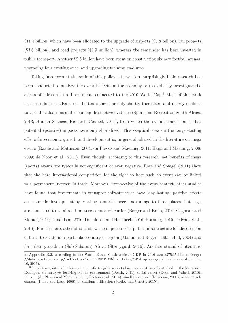
Taking into account the scale of this policy intervention, surprisingly little research has

been conducted to analyze the overall effects on the economy or to explicitly investigate the

effects of infrastructure investments connected to the 2010 World Cup.3 Most of this work

has been done in advance of the tournament or only shortly thereafter, and merely confines

to verbal evaluations and reporting descriptive evidence (Sport and Recreation South Africa,

2013; Human Sciences Research Council, 2011), from which the overall conclusion is that

potential (positive) impacts were only short-lived. This skeptical view on the longer-lasting

effects for economic growth and development is, in general, shared in the literature on mega

events (Baade and Matheson, 2004; du Plessis and Maennig, 2011; Hagn and Maennig, 2008,

2009; de Nooij et al., 2011). Even though, according to this research, net benefits of mega

(sports) events are typically non-significant or even negative, Rose and Spiegel (2011) show

that the hard international competition for the right to host such an event can be linked

to a permanent increase in trade. Moreover, irrespective of the event context, other studies

have found that investments in transport infrastructure have long-lasting, positive effects

on economic development by creating a market access advantage to those places that, e.g.,

are connected to a railroad or were connected earlier (Berger and Enflo, 2016; Cogneau and

Moradi, 2014; Donaldson, 2016; Donaldson and Hornbeck, 2016; Hornung, 2015; Jedwab et al.,

2016). Furthermore, other studies show the importance of public infrastructure for the decision

of firms to locate in a particular country or region (Martin and Rogers, 1995; Holl, 2004) and

for urban growth in (Sub-Saharan) Africa (Storeygard, 2016). Another strand of literature

in Appendix B.2. According to the World Bank, South Africa’s GDP in 2010 was $375.35 billion (http://data.worldbank.org/indicator/NY.GDP.MKTP.CD/countries/ZA?display=graph, last accessed on June16, 2016).

3 In contrast, intangible legacy or specific tangible aspects have been extensively studied in the literature.Examples are analyses focusing on the environment (Death, 2011), social values (Desai and Vahed, 2010),tourism (du Plessis and Maennig, 2011; Peeters et al., 2014), small enterprises (Rogerson, 2009), urban devel-opment (Pillay and Bass, 2008), or stadium utilization (Molloy and Chetty, 2015).

2

deals with the impact of place-based policies on regional economic development and finds

positive effects in both the short- and the long-run (Becker et al., 2010, 2012; Kline and

Moretti, 2014). Carrying over these arguments to the World Cup context, one particularly

can expect transport infrastructure investments made for the tournament to have exerted

significantly positive and long-lasting economic effects.

Given the scarcity of evidence with respect to such important issues, there is a need for

a thorough re-assessment of the 2010 World Cup that is able to provide a more detailed

picture. The present paper fills this gap and makes several contributions to the literature. To

begin with, we are first to present causal evidence on the overall economic influence of the

tournament. Our study also allows to track the effect at different time horizons starting in

2004, when South Africa was announced the host country of the 2010 World Cup.

Second, we resort to night lights intensity (luminosity) data, that have been recently ac-

knowledged in the literature as a suitable proxy for economic development (Henderson et al.,

2012; Michalopoulos and Papaioannou, 2014). Data on night lights are collected by satellites

and are available for the whole globe at a high level of geographical precision.4 Therefore, their

usefulness as an economic proxy is of particular relevance in the case of developing countries,

where administrative data on GDP or other economic indicators are often of bad quality, not

given for a longer time span, and/or not provided at a desired sub-national level. We harness

this advantage of the luminosity data, which enables us to precisely identify the effects in

treated regions of the country, i.e., regions affected by the investments related to the World

Cup, in that we can easily extract information for a chosen, sometimes very small adminis-

trative unit. In particular, we conduct our analysis both by looking across municipalities and

also within municipalities—using information on the next smaller unit, i.e., electoral districts

(so-called wards). Variation in the data on this very dissected administrative level enables us

to precisely localize specific interventions and depict potential heterogeneity across treatment4 The economic literature using high-precision satellite data, also on other outcomes than night lights, is

growing. For instance, Axbard (2016) exploits satellite data on specific oceanographic conditions to study theeffect of fishermen’s income opportunities on sea piracy. Groger and Zylberberg (2016) use geophysical satellitedata while analyzing whether internal labor migration facilitates shock coping in rural economies.

3

effects.

Third, precise identification of such World Cup effects was only possible due to thorough

research on infrastructure investments conducted in South Africa for the time span 2004–2013

(our treatment period). As a result of this research, we have created a comprehensive list

encompassing 127 investment projects divided into different categories: airports, stadiums,

roads, rail, public transport, etc. To the best of our knowledge, such an attempt to summarize

investment projects in South Africa in a particular time span has never been undertaken before.

The investment list can also act as a stand-alone document and be useful for researchers dealing

with South Africa in other regards. Based on this full list, we have selected as treatments for

our analysis those 72 projects which, according to the information sources, are clearly classified

as World Cup related and could be localized.

Fourth, we evaluate such treatments by applying synthetic control methods (SCM), an ap-

proach introduced by Abadie and Gardeazabal (2003) and Abadie et al. (2010). SCM provides

intuitive identification of causal effects by comparing an appropriate counterfactual to the ac-

tual development of the outcome after the intervention. The counterfactual is constructed

by an algorithm-derived combination of optimally weighted comparison units, which best re-

semble the characteristics of the treated one according to economic predictors pre-treatment.

Hence, one great advantage of SCM is that it is not based on ad hoc choices of control units.

Instead, it lets the data speak regarding the selection and respective weights of control units,

which is particularly helpful in the presence of many potential candidates, like municipalities

or electoral districts. SCM has already proven successful in the quantification of treatment

effects across a wide range of fields.5 However, to the best of our knowledge, this paper is the

first one that employs SCM in the context of mega (sports) events. Moreover, by combining

SCM with night lights intensity data, we offer a framework for evaluation of various policy

programs aimed at stimulating economic growth, especially—but not solely—in developing

countries.5 See, for instance, Cavallo et al. (2013) (natural disasters), Kleven et al. (2013) (taxation of athletes),

Gobillon and Magnac (2016) (enterprise zones), Acemoglu et al. (2015) (political connections), or Pinotti(2015) (crime).

4

Finally, to facilitate the interpretation of our SCM results, we translate the obtained lu-

minosity effects into values expressed in terms of standard economic outcomes, which policy

makers are usually more interested in. For that purpose, we derive unemployment, GDP, and

income effects by using corresponding conversion factors obtained through OLS regressions.

Importantly, by converting night light impacts into effects in terms of the unemployment rate,

we go beyond the existing literature which so far has only explored the relationship between

night lights and GDP per capita or income per capita (Henderson et al., 2012; Pinkovskiy

and Sala–i–Martin, 2016). The reason for choosing the unemployment rate is that, in South

Africa, it is available at a finer regional level than GDP and thus offers a more precise basis for

deriving a conversion factor. We additionally consider GDP and income as reference economic

measures for the sake of completeness and to compare our conversion factors to those of the

related literature.

The findings of this paper show a considerable difference between short- and longer-run

effects associated with the tournament, and point to the sources of these differences. Based on

the average World Cup venue on municipality level, we find a significant and positive short-run

impact between 2004 and 2009, that is equivalent to a 1.3 percentage points decrease in the

unemployment rate or an increase of around $335 GDP per capita. Taking the costs of the

investments into account, we derive a net benefit of $217 GDP per capita. Starting in 2010,

the average effect becomes insignificant. However, by zooming in on respective municipalities

and using variation on the next finer level (wards), we are able to show that the average

picture obscures heterogeneity related to the sources of economic activity and the locations

within the treated municipalities. More specifically, we demonstrate that around and after

2010, there has been a positive, longer-run economic effect stemming from new and upgraded

transport infrastructure. These positive gains are particularly evident for smaller towns, which

can be explained with a regional catch-up towards bigger cities. For example, in Rustenburg—

one of the smaller World Cup venues—we find a very large effect of the World Cup related

investment equivalent to an increase in GDP per capita of around $3, 642, what is roughly the

5

difference between the GDP per capita of the richest province and the average one. Contrarily,

the effect of stadiums is generally less significant and no longer-lasting economic benefits are

attributed to the construction or upgrade of the football arenas. Those are merely evident

throughout the pre-2010 period. Importantly, our results appear not to be simply driven by

the light of airports or stadiums themselves and they are insensitive to a battery of robustness

checks, like altering the set of covariates, differently composed synthetic control groups, or

different definitions of the treatment group. Eventually, our findings underline the importance

of investments in transport infrastructure, particularly in rural areas, for longer-run economic

prosperity and regional catch-up processes.

The remainder of this paper is organized as follows. Section 2 gives details on the 2010

World Cup, describes the night lights data set, and provides first descriptive evidence. In

Section 3, we outline the SCM approach and how we derive conversion factors to translate our

SCM estimates into standard economic measures. Section 4 presents and discusses the findings

of the empirical analysis on different levels of aggregation. Finally, Section 5 concludes.

2 Background of the Analysis and Data

2.1 The 2010 World Cup in South Africa

On May 15, 2004, the FIFA executive committee announced its decision to award the 2010

mens’ football World Cup to South Africa. This 19th FIFA World Cup, taking place between

June 11 and July 11, 2010, was the first such tournament being hosted on the African continent.

The matches were allocated across 10 stadiums located in nine different cities: Bloemfontein

(Mangaung Metropolitan Municipality), Cape Town (City of Cape Town Metropolitan Mu-

nicipality), Durban (eThekwini Metropolitan Municipality), Johannesburg with two stadiums

(City of Johannesburg Metropolitan Municipality), Nelspruit (Mbombela Local Municipality),

Polokwane (Polokwane Local Municipality), Port Elizabeth (Nelson Mandela Bay Metropoli-

tan Municipality), Pretoria (City of Tshwane Metropolitan Municipality), and Rustenburg

6

(Rustenburg Local Municipality). The corresponding venues constitute our treated munici-

palities.

These municipalities are scattered across eight (out of all nine) provinces and nine (out

of all 52) districts, which differ with respect to their economic performance and the regional

distribution of sectors. Johannesburg and Pretoria lie in the province Gauteng, whose average

real annual growth rate of 4.6% in the periods 2001–2011 and contribution of about 34% to

the overall South African economic activity are the highest across all nine provinces. Gaut-

eng’s contribution to the South African output in manufacturing, construction, and finance

amounted (in 2011) to 40.5%, 43.3%, and 41.1%, respectively. A counterexample to Gauteng

is the province Limpopo (with Polokwane as one of the World Cup venues), that recorded an

average annual real growth rate of 3.2% in 2001–2011 and 6.5% average contribution to the

country’s GDP. While the contribution of Limpopo to the South African manufacturing sector

amounted to only 1.5%, the province plays (with 23.7%) a very important role in the mining

and quarrying sector. As regards the socio-economic situation of the World Cup municipalities,

some of them are large centers, like the City of Johannesburg Metropolitan Municipality or

the City of Cape Town Metropolitan Municipality, both with around three million inhabitants

and the average household income in 2001 of $12,317. This is in contrast to smaller municipal-

ities among the World Cup venues (population mostly less than 200, 000), e.g., the Polokwane

Local Municipality or the Mbombela Local Municipality, where the average household income

in 2001 amounted to about $5,200.6

It is important to note that we consider the treatment to begin in 2004, when the Inter-

national Football Federation officially selected South Africa over Egypt and Morocco as the

host country. After this date, a battery of preparations, like the construction and upgrade of

new and existing stadiums, the renewal and extension of transport infrastructure, the con-6 Socio-economic data for the City of Johannesburg Metropolitan Municipality, Polokwane Local Mu-

nicipality, and Mbombela Local Municipality are taken from the Census 2011 Municipal Reports (down-load at: http://www.statssa.gov.za/?page_id=3955; last accessed on January 19, 2016). Data on provin-cial economic activity are retrieved from the document of Statistics South Africa available at: http://www.statssa.gov.za/economic_growth/16%20Regional%20estimates.pdf; last accessed on January 19,2016.

7

struction of hotels, etc., began.7 Overall, the South African investments totaled about $14

billion, of which $11.4 billion were spent on transport and communication infrastructure. An

example for a major investment in transport infrastructure is the construction of King Shaka

International Airport in Durban that cost around $930 million. The largest investment in

sports infrastructure was the First National Bank Stadium (aka Soccer City) in Johannes-

burg, hosting the opening and final game, that underwent major refurbishments and upgrades

(i.a., extension of capacity to 94, 736 seats) for a total of $451.6 million that were shared by

the central government, the provincial government, and the municipality.8

2.2 Data Set

In the subsequent empirical analysis, we will consider municipalities and wards (electoral dis-

tricts) as observational units. Panel (a) of Figure 1 shows all 234 South African municipalities

including the nine venues of the 2010 World Cup colored in gray. Municipal borders are drawn

according to a shapefile downloaded from the DIVA-GIS website.9 The map also comprises the

country of Lesotho (the large white area in the middle-right of the map), a landlocked country

considerably less developed than South Africa. Panel (b) of Figure 1 depicts all 4, 277 South

African wards and the World Cup municipalities indicated by bold-type, light-blue borders.

The variable of interest in our analysis is economic development as proxied by the night

light intensity (luminosity) of an observational area. We resort to luminosity since, in South

Africa, GDP data are only available for the nine provinces but not for municipalities or

wards. Furthermore, luminosity is widely used as proxy for economic development, especially

in countries where GDP data are either not available or of bad quality (Henderson et al., 2012;7 To the best of our knowledge, there were no significant investments related to the 2010 World Cup

undertaken before 2004, e.g., during the bidding process. We test for this throughout our robustness checks inAppendix A and find our assumption to be confirmed.

8 Capacity figures are taken from Chapter four of the FIFA World Stadium Index, available here: http://www.playthegame.org/fileadmin/documents/world_stadium_index_4_fifa_wc.pdf, last accessed onFebruary 5, 2016. Information on overall expenditures and costs regarding the two mentioned projects isprovided in Appendix B.2.

9 Downloadable at: http://biogeo.ucdavis.edu/data/diva/adm/ZAF_adm.zip, last accessed on January19, 2106.

8

(a) South African Municipalities and World CupVenues

(b) South African Wards and World Cup Venues

Note: Panel (a) shows the municipalities of South Africa and the World Cup venues depicted in gray. Panel (b) shows the SouthAfrican wards and the World Cup venues depicted in light-blue.

Figure 1: Municipalities, Wards, and World Cup Venues in South Africa

Hodler and Raschky, 2014; Lessmann and Seidel, 2015; Michalopoulos and Papaioannou, 2014;

Mveyange, 2015; Elliot et al., 2015; Wahl, 2016). It is found to be highly correlated with GDP

per capita and other measures of prosperity, like electricity provision (Baskaran et al., 2015;

Min et al., 2013), and can therefore be considered as a valid proxy (Chen and Nordhaus,

2011; Henderson et al., 2012).10 In the context of our study, night light luminosity is expected

to correspond to, e.g., buildings of firms that settle next to newly founded infrastructure,

construction activity done at night, private buildings in newly created settlements around

the treatment areas, or the upgrade and refurbishment of existing buildings and industrial

facilities. Such expectations are supported by the literature, according to which night lights

are related with, among others, the expensiveness of roofing material (Jean et al., 2016) or

the number and density of industrial facilities as well as wages in a grid cell (Mellander et al.,

2015).

Night light intensity is measured by an integer ranging from 0 (unlit) to 63. The data are

made available by the National Geophysical Data Center (NGDC) of the National Oceanic and

Atmospheric Administration of the U.S., and originate from images taken by satellites of the10 Limitations of luminosity as a proxy for economic development are discussed, among others, in Kulkarni

et al. (2011).

9

Defense Meteorological Satellite Program (DMSP) of the U.S. Department of Defense. We use

shapefiles containing the average visible, stable nighttime lights and cloud-free coverage, where

ephemeral events (fires, etc.) as well as background noise are removed and only light from sites

with persistent lightning is included.11 Night light intensity data are available on pixel (grid

cell) level, with each pixel corresponding to 30x30 arc seconds, i.e., one value represents the

average night light intensity of an area of 0.86 square kilometer (on the equator). Moreover,

data are available for each of the 22 years between 1992 and 2013, leaving us with a panel

data set of 5, 148 municipality-year pairs and 92, 884 ward-year pairs, respectively.12 Panel (a)

of Figure 2 shows the spatial distribution of pixel level luminosity in South Africa in 2013.

Municipal borders are colored in light-blue and the World Cup venues are depicted in bold-

type red.

For our empirical analysis, luminosity data are aggregated from pixel level to the respective

observational unit by averaging the pixel values in the area of each municipality/ward and

assigning this value to the respective (whole) area.13 Panel (b) of Figure 2 shows the distribu-

tion of average luminosity across South African municipalities in 2013. The nine municipalities11 We use the latest version (4.0) of the data. It can be downloaded at: http://ngdc.noaa.gov/eog/dmsp/

downloadV4composites.html, last accessed on January 19, 2016. A common problem with these data is thatthe light of gas flares is included and could be mistaken for lights of settlements. However, in the area studiedin this paper, no gas flares exist.

12 From all 4, 277 wards, we are able to use 4, 222 of them in the empirical analysis as some wards are toosmall to calculate exact luminosity or elevation values. When using the luminosity series pooled over time, apotential issue is that a portion of the temporal variation in the data can be due to the fact that this data iscollected by different satellites, which are not calibrated on a common level. To make luminosity values morecomparable over satellites, the data can be inter-calibrated manually following, e.g., a procedure suggested byElvidge et al. (2009). However, Chen and Nordhaus (2011) find that results only marginally change when usinginter-calibrated luminosity. In line with this, after inter-calibrating our data set based on the values given byElvidge et al. (2014), we find a correlation with the original data of 0.991. Consequently, for our empiricalanalysis, inter-calibration did not affect our results noticeably.

13 Alternatively, we could have drawn on luminosity per capita. However, population figures on municipalityor ward level are only available for a very few years throughout our observation period, which would leadto distinctly reduced number of observations. The same problem occurs with alternative luminosity data—the so-called ’radiance calibrated at night data’ (available at: http://ngdc.noaa.gov/eog/dmsp/download_radcal.html, last accessed on January 19, 2016), that has been used by, e.g., Gonzalez-Navarro and Turner(2016). This data does not feature the cap at 63, but comprises seven cross sections, out of which only threecorrespond to the analyzed post-treatment time span 2004–2013 (2004, 2006, 2011). Furthermore, the literaturesometimes uses the log of luminosity as dependent variable in OLS regressions (Henderson et al., 2012; Hodlerand Raschky, 2014). Usually, this is done because the distribution of night lights is skewed with small valuesof luminosity being most frequent. However, for our SCM analysis to be valid, it is not necessary that theoutcome of interest is normally distributed, so we follow Elliot et al. (2015) and Strobl and Valfort (2015)using untransformed levels of luminosity.

10

(a) Pixel Level Distribution of Luminosity (b) Municipal Average of LuminosityNote: Panel (a) shows pixel level luminosity with municipality borders (colored in light-blue) and World Cup venues (coloredin bold-type red). Luminosity is depicted by colors ranging from black (unlit) to white (level 63). Panel (b) shows the averageluminosity of a municipality and the World Cup venues depicted by bold-type borders. Average luminosity of a municipality isdepicted by colors ranging from white to dark blue, where darker colors indicate higher luminosity.

Figure 2: Pixel and Average Municipality Level Distribution of Luminosity in 2013

hosting the 2010 World Cup are indicated by bold-type borders. Luminosity ranges from 0.01

in the Mier Local Municipality (Province North Cape),14 that is almost unsettled, to 57.3

in the Johannesburg Metropolitan Municipality. Luminosity is, in general, larger in coastal

municipalities and in the north, where also the largest agglomerations and the most important

economic centers of South Africa can be found. This supports its validity as an indicator of

economic development.

2.3 Descriptive Evidence

A descriptive look at the temporal development of luminosity between 1992 and 2013 can

provide us with some first suggestive evidence regarding the effect of the FIFA announcement

on economic development across the nine hosting municipalities. If there is a positive effect

of this treatment in 2004, or follow-up treatments thereafter, we should see an increase in

luminosity somewhere between 2005 and 2010. Figure 3 depicts luminosity as a time series14 Especially within the municipalities located in the western South African wastelands, there exist pixels

which are zero throughout the entire sampling period. In one of the robustness checks in Appendix A, wefollow Elliot et al. (2015) and remove such pixels prior to the aggregation on municipal level. Correspondingestimation results stay almost exactly identical to our baseline ones including the zero pixels.

11

1416

1820

2224

Lum

inos

ity

1990 1995 2000 2005 2010 2015Year

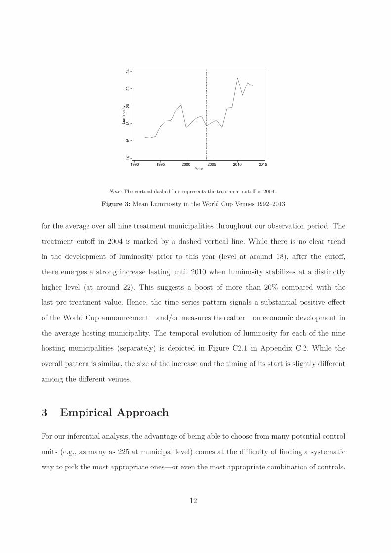
Note: The vertical dashed line represents the treatment cutoff in 2004.

Figure 3: Mean Luminosity in the World Cup Venues 1992–2013

for the average over all nine treatment municipalities throughout our observation period. The

treatment cutoff in 2004 is marked by a dashed vertical line. While there is no clear trend

in the development of luminosity prior to this year (level at around 18), after the cutoff,

there emerges a strong increase lasting until 2010 when luminosity stabilizes at a distinctly

higher level (at around 22). This suggests a boost of more than 20% compared with the

last pre-treatment value. Hence, the time series pattern signals a substantial positive effect

of the World Cup announcement—and/or measures thereafter—on economic development in

the average hosting municipality. The temporal evolution of luminosity for each of the nine

hosting municipalities (separately) is depicted in Figure C2.1 in Appendix C.2. While the

overall pattern is similar, the size of the increase and the timing of its start is slightly different

among the different venues.

3 Empirical Approach

For our inferential analysis, the advantage of being able to choose from many potential control

units (e.g., as many as 225 at municipal level) comes at the difficulty of finding a systematic

way to pick the most appropriate ones—or even the most appropriate combination of controls.

12

Difference-in-Differences (DiD) approaches, seemingly suitable in a setting as ours, offer too

much leeway in choosing the respective control unit, giving room for manipulation and ques-

tioning the external validity of corresponding results. Moreover, the common trend assumption

needed for identification might be too restrictive in our context. Therefore, we employ an al-

ternative identification strategy which, in contrast to DiD, still delivers reliable results when

the common trend assumption is violated or when unobserved confounders vary with time:

synthetic control methods (SCM). In Section 3.1, we will describe some theory related to the

SCM approach, explaining how treatment effects can be derived in a general setting. Since

policy makers are typically interested in more standard economic variables than luminosity,

we want to make the interpretation of our prospective SCM results more straightforward. In

Section 3.2, we will therefore show how to obtain suitable conversion factors, which can then

serve to translate estimated SCM results of the World Cup expressed in luminosity into effects

in terms of unemployment, GDP, and income.

3.1 Synthetic Control Methods

SCM, an approach introduced in Abadie and Gardeazabal (2003) and Abadie et al. (2010), is

based on the idea that an optimally weighted average of available control units (comprising

the so-called donor pool) is able to reproduce the trajectory of the outcome of interest of the

treated unit in absence of the treatment. The treatment effect can then be calculated by taking

the difference between the actual outcome of the treated unit in the post-intervention period(s)

and the respective outcome of the so-called synthetic unit, i.e., the counterfactual built from

the donor pool. Using an appropriate set of economic predictors and pre-treatment outcomes,

SCM select the synthetic unit as the optimally weighted average of such comparison units that

best resemble the characteristics of the respective treated one prior to the intervention. This

yields unbiased identification of the causal effect of interest, even if treatment assignment is

based on unobservable factors whose effects vary over time.

More formally, suppose that there exist J + 1 units, indexed by i, and T time periods,

13

denoted by t. The univariate outcome of interest Yit is observed for all units i ∈ {1, ..., J + 1}in all time periods t ∈ {1, ..., T}, and the treatment takes place in period T0 such that the

data can be divided into a pre-treatment period with t < T0, and a post-treatment period

with t ≥ T0. For simplicity, assume that only the first unit i = 1 is treated. Following the

potential outcome framework, we are interested in estimating a series of treatment effects on

the treated, given as τ1t = Y1t − Y1t(0) for t ≥ T0, with Y1t being the actual outcome of the

treated unit at time t, and Y1t(0) being the hypothetical outcome for the treated unit at time

t in absence of the treatment. It is now assumed that the potential outcome in absence of the

treatment is given by:

Yit(0) = θtZi + ηit with ηit = δt + λtμi + εit, (1)

where Zi is a (r × 1) vector consisting of r observable characteristics with predictive power

for the outcome of interest. θt illustrates that these outcome-relevant characteristics are not

restricted to being time-constant.15 The error term ηit is decomposed into an unknown period-

specific factor δt common to all units, an (F × 1) vector of unobservable unit-specific factors

μi, whose effect may vary over time, and a unit- and time-specific transitory shock εit with

E(εit) = 0, being independently and identically distributed across units.16 Under standard

assumptions and with a sufficient number of pre-intervention periods (Abadie et al., 2010),

the estimator for the treatment effects is given as:

τ ∗1t = Y1t −

J+1∑i=2

w∗i Yit for t ≥ T0, (2)

if there exists a weighting vector W ∗ = (w∗2, ..., w∗

J+1)′, with w∗i ≥ 0 and w∗

2+...+w∗J+1 = 1, such

that the observable and unobservable characteristics of the treated unit can be reconstructed15 However, if these characteristics vary over time, the usual proceeding in the literature is to build averages

over time. Contrarily, Kloßner and Pfeifer (2015) develop an extended SCM approach allowing to incorporatewhole time series of such characteristics.

16 Note that λtμi can also be interpreted as relaxing the common trend assumption and, moreover, if λt (a(1 × F ) vector of unknown common factors) is constant over time, the model collapses to a DiD approach.

14

by a weighted average of the controls. As μi is a vector of unobserved factors, the idea of SCM

is to match on pre-intervention outcomes in addition to the observables Zi.

For the implementation of the SCM estimator, define a (k × 1) column vector X1 =

(Z ′1, Y

L11 , ..., Y

LM

1 )′ containing the (average) values of the observable characteristics as well

as M linear combinations of the pre-intervention outcomes for the treated unit. Each of

these M linear combinations corresponds to a ((T0 − 1) × 1) vector L = (l1, l2, ..., lT0−1)′

with YL

1 = ∑T0−1t=1 ltY1t. Analogously, define the (k × J) matrix X0 to be the counter-

part of X1 for the unexposed units. The standard SCM method chooses W to minimize√

(X1 − X0W )′V (X1 − X0W ), with V being a positive semi-definite diagonal (k × k) matrix,

whose elements are the weights reflecting their relative predictive power. The most common

approach to determine V is a data-driven procedure proposed by Abadie and Gardeazabal

(2003) and Abadie et al. (2010): it chooses V among all positive definite and diagonal ma-

trices such that the root mean squared prediction error (RMSPE) of the outcome variable is

minimized over the pre-intervention periods.17

Thus, the main task of SCM is to find non-negative control unit weights W , summing up

to unity, for given predictor weights V such that:

minW

√(X1 − X0W )′V (X1 − X0W ), (3)

while we denote the solution to this problem by W ∗(V ).

3.2 Converting Night Lights into Standard Economic Outcomes

When translating our prospective SCM effects expressed in luminosity into those expressed in

terms of standard economic outcomes, we resort to three such variables: the unemployment17 When analyzing the new cross-validation method proposed by Abadie et al. (2015), which is supposed to

determine predictor weights V , Kloßner et al. (2016) show that this method is flawed since it hinges on predictorweights which are not uniquely defined and, consequently, might lead to ambiguous estimation results. Thisis why, in the following, we abstain from using cross-validation techniques and stick to the ‘standard’ SCMframework.

15

rate, GDP per capita, and income per capita.18 For each of these three measures, we obtain a

corresponding conversion factor by estimating an OLS regression using the respective outcome

as the dependent variable and luminosity as the regressor of interest. If applicable, we include

district/municipality and year fixed effects as well as several controls (area, distance to railway,

elevation, soil quality).

First, we estimate the following regression equation for the conversion of night light effects

into unemployment:

UNijk,t = α + βNLijk,t + θk + λt + εijk,t, (4)

where UNijk,t and NLijk,t are the unemployment rate and night light luminosity, respectively,

in province i, district j, municipality k, and year t. θk denotes municipality fixed effects,

whereas λt describes year fixed effects introduced to account for the business cycle, and εijk,t

is the error term. The coefficient of the luminosity measure β is the conversion factor.

Second, as GDP per capita is only available on province level, the respective conversion

factor is computed based on the estimation of a modified specification. Here, GDP per capita

and luminosity vary on province level, while the control variables are still given on municipality

level:

GDPi,t = α + βNLi,t + γ′Xijk + λt + εijk,t, (5)

where GDPi,t and NLi,t are GDP per capita and luminosity, respectively, in province i in year

t. Xijk denotes the controls in province i, district j, and municipality k. λt and εijk,t are as in

Equation (4).

Finally, income per capita is available on municipality level, but solely for the year 2007.

Consequently, we cannot include year or municipality fixed effects when estimating the con-

version factor from luminosity to income per capita. Formally, we thus estimate the following

equation:

INCijk,t = α + βNLijk,t + γ′Xijk + θj + εijk,t, (6)18 Sources and exact definitions of all variables are available in Appendix B.1. A descriptive overview of the

data is provided in Table C1.1.

16

Table 1: Relationship between Night Lights and Economic Outcomesa)

Characteristics/ Dependent Variable

Regressors Unemployment Rate GDP per capita Income per capita

(1) (2) (3)

Level of Variation Municipality Province Municipality

Years in Sample 1996, 2001, 2007, 2011 1996, 2001, 2007 2007

Luminosity −0.723** 1, 400.699*** 911.555***

(0.282) (38.543) (270.819)

Conversion Factorb) −0.723 191.690 124.749

District Dummies No No Yes

Municipality Dummies Yes No No

Year Dummies Yes Yes No

Controls No Yes Yes

Observations 936 702 234

R2 0.819 0.555 0.509a) Robust standard errors are reported in parentheses. Coefficient is statistically differentfrom zero at the ***1%, **5%, and *10% level. Unit of observations in all three columns isa municipality. However, the dependent variable and luminosity do only vary on provinciallevel in Column (2). The set of controls includes a municipality’s area in square kilometers,its distance to the closest railway, its elevation, and soil quality. Each regression includes aconstant not reported.b) Conversion factors related to GDP per capita and income per capita are obtained by trans-lating the corresponding luminosity effects expressed in the national currency ‘Rand’ into U.S.dollars ($) using the average exchange rate of 2010.

where INCijk,t is income per capita in province i, district j, municipality k, and year t,

NLijk,t denotes the corresponding night lights, and θj are district fixed effects. The remainder

is analogous to Equations (4) and (5).

The results of the OLS estimations are summarized in Table 1. Column (1) provides

the estimates of Equation (4): we find a statistically significant conversion factor of −0.723,

implying that a one unit increase in luminosity translates into a reduction in the unemployment

rate of 0.723 percentage points. Column (2), corresponding to Equation (5), yields a conversion

factor of around 1, 401, meaning that a one unit increase in luminosity increases the provincial

GDP per capita by around 1, 401 Rand ($192). As the average provincial GDP per capita is

$3, 680 and its standard deviation is $1, 345, an increase by $192 seems to be a reasonable

quantity. If we alternatively regress logarithmized GDP per capita on logarithmized luminosity,

we end up with an estimated elasticity of around 0.21, what is broadly in line with—but at

the lower end of—elasticities found by other studies (Henderson et al., 2012; Lessmann and

17

Seidel, 2015).19 Finally, in Column (3), we estimate Equation (6), resulting in a conversion

factor of 911.555. Hence, a one unit increase in luminosity is equivalent to an increase in per

capita income of around 912 Rand ($125).

4 Estimation Results and Effect Heterogeneity

A major aspect and prerequisite with respect to our study is the identification of municipalities

and wards treated by the measures designated for the World Cup. To do this in a systematic

way, we have first detected all projects potentially relevant for our analysis, i.e., those projects

which were conducted in South Africa during the period from 2004 (our treatment start) until

2013 (when our sample ends). In so doing, we have considered four different project types:

construction and upgrade of (i) railway, metro, and bus stations, (ii) airports, (iii) stadiums

(main World Cup stadiums and training stadiums), and (iv) water infrastructure (e.g., dams

or pipelines). We have collected a list of such projects, including (when available) information

on their location, construction period, and costs. Overall, we have identified 127 different

infrastructure projects. Since, in the subsequent empirical analysis, we will focus on World

Cup related projects only, this leaves us with 72 projects in overall 16 municipalities.20 Out

of those 72 projects, 61 took place in nine World Cup venues and 11 in seven non-World Cup

venues. Throughout our baseline analysis that assumes World Cup venues as the only treated

municipalities, we will therefore consider 61 projects as treatments.21

In the first step of this analysis (Section 4.1), we will look at the average luminosity of

World Cup venues at municipality level. To be more specific, we will pool luminosity for all19 If we follow Pinkovskiy and Sala–i–Martin (2016) and estimate the elasticities of luminosity with respect

to GDP per capita instead, we arrive at an elasticity of around 1 (1.17), which is roughly what they find intheir baseline estimates.

20 A list reporting these 72 projects, information on them, as well as the sources of the information, is avail-able in Appendix B.2. The full list including 127 projects can be downloaded at: http://www.martynamarczak.com/research/SA_AllProjects.pdf.

21 Note that in one of the robustness checks in Appendix A, we extend the treated units by the seven non-World Cup venues affected by World Cup investments, and thus include all 72 projects in the set of treatments.The remaining 55 projects from the whole set of 127 projects were not World Cup related, or we are not ableto gather enough information to be sure that they are directly related to the World Cup, to locate them, orthey were not even partly finished.

18

World Cup municipalities using the arithmetic mean and then conduct a single-case study

applying SCM, which will result in a treatment effect given in the average World Cup venue’s

luminosity.22 Additionally, we have to exclude potential spillovers from treated regions to non-

treated ones as these would invalidate the identifying assumptions of SCM. We do this, as

is standard in the regional policy evaluation literature (Alder et al., 2016; Aragon and Rud,

2015; Becker et al., 2010; Dettmann et al., 2016), by considering spillovers to be a function of

proximity to the treated locations and, hence, exclude regions neighboring World Cup venues

(and Lesotho) from the donor pool. Under the hypothesis of no indirect effects on non-treated

regions, using a donor pool stemming from the same country as the treated unit does should be

a first best solution, since this offers better comparability than a donor pool from any another

country.23 However, this also implies that we are not after quantifying or explicitly modeling

spillover effects, which would also require a different identification approach. Contrarily, we are

solely interested in the direct effects of the World Cup and its related infrastructure projects.

In a second step (Section 4.2), we will zoom in on several treated wards within a particular

treated municipality, which, e.g., harbor a stadium or an airport, and for which we expect

heterogeneous effects depending on the type of infrastructure as well as the size and location of

the respective city. Using information on 72 treatments, we are able to localize 102 wards that

are affected by World Cup measures. 85 of these wards are located within a World Cup venue

and 17 within a non-World cup venue.24 Throughout these SCM analyses, we will consider22 An alternative approach would be to conduct a respective SCM study for each of the treated units and

subsequently pool over the individual treatment effects as it is done in, e.g., Acemoglu et al. (2015) or Dubeand Zipperer (2015). In their pooling procedure, Acemoglu et al. (2015) re-weight the individual treatmenteffects based on the goodness of the pre-treatment fit for the corresponding treated unit. Dube and Zipperer(2015) pool over multiple case studies using the mean percentile rank.

23 However, we also conduct the municipality level SCM analysis using alternative donor pools from twoother countries, respectively: Mozambique, a neighboring country of South Africa, and Morocco, a country inNorthern Africa that also applied for hosting the 2010 World Cup. Detailed information on these countries,the composition of the corresponding synthetic unit, as well as the obtained results and their discussionare presented in Appendix A.2. For both alternative donor countries, we find a positive, albeit insignificanttreatment effect, presumably stemming from the fact that the synthetic unit does not sufficiently representthe case of the average World Cup venue in South Africa.

24 Especially in the Gauteng province, some wards have more than one treatment so that the number oftreatment wards is not identical to the number of treatments identified. The location of the treatments isassigned according to the coordinates given by wikipedia, http://www.geonames.org, google maps, and thewebsite http://www.mbendi.com (for railway and metro stations); last accessed on January 19, 2016.

19

treated wards in a given treated municipality separately. This is in contrast to our study at

municipality level, where the subject of the analysis is the average effect over all World Cup

venues. Analogous to the study at municipality level, however, we will exclude neighbors of the

respective treatment ward and all other treatment wards including their neighbors within the

same municipality (to ensure that there are no spillovers).25 Finally, regarding the conversion

of our SCM estimates, we have to note that the three outcomes of interest (as reported in

Table 1) are not available on ward level. This makes a respective conversion in Section 4.2

somewhat less precise since the underlying conversion factor stems from municipality level

data.

4.1 The Average World Cup Venue

As we have 234 municipalities in South Africa, out of which there are nine ‘treated’ ones,

the potential donor pool J consists of 225 non-treated municipalities. However, to avoid the

problem of potential spillovers that could result from the proximity to the treatment, we will

exclude from the donor pool all municipalities directly neighboring a respective treated one

(45) or bordering Lesotho (14). Additionally, we will exclude those seven municipalities with

World Cup related infrastructure projects (airports and training stadiums) that were no World

Cup venues (like Buffalo City Metropolitan Municipality or George Local Municipality) and

their respective neighbors (28).26 This leaves us with a donor pool consisting of 131 control

units. Moreover, throughout our analysis, we will use pre-treatment averages of the following

economic predictors: area of municipality in square kilometer, distance to next railway in

kilometer, average elevation of municipality above sea level in meters, 2001 share of people25 Overall, there are 336 such neighboring wards, whose quantity varies across municipalities.26 This should yield a compromise to the ‘dilemma’ discussed in Gobillon and Magnac (2016): on the one

hand, choosing areas in the neighborhood of treated areas as controls might be problematic due to spilloversor contamination effects; on the other hand, non-neighbors might be located too far away from the treatedareas to be good matches and therefore good controls. Note, however, that we relax such exclusion rulesthroughout our sensitivity checks reported in Appendix A. Also note that there is a significant amount ofoverlap between municipalities neighboring a World Cup venue and another municipality with World Cupmeasures. In above figures, those are allocated to the neighbors of the World Cup venues. Municipalitiesneighboring both Lesotho and one of the municipalities with World Cup related investments (either a WorldCup venue or another affected municipality) are counted as neighboring Lesotho.

20

with indigenous heritage per municipality, 2001 share of people with tertiary education per

municipality, average municipality’s soil quality, and the 2001 percentage of people unemployed

in municipality.27 Those variables are chosen because they were identified as robust predictors

of luminosity and regional development by previous studies (Gennaioli et al., 2013, 2014;

Henderson et al., 2016) and because they reflect the particular determinants of agglomeration

and development in South Africa.28

Synthetic Unit

Our municipality level SCM analysis finds a combination of non-treated units that sufficiently

replicates the luminosity evolution of the average World Cup venue before the official FIFA

announcement in 2004—the corresponding RMSPE is 0.877. To be more specific, the average

World Cup venue is synthesized by the following municipalities: Msunduzi, uMhlathuze, and

Govan Mbeki, which are attributed w-weights of about 3.5%, 80.8%, and 15.7%, respectively.29

Before discussing our SCM results based on the graphical representation depicted in Figure 4,

we have a more detailed look at the three weighted municipalities in order to show that their

combination provides a plausible counterfactual for the average World Cup venue.

The uMhlathuze Local Municipality, that obtains by far the greatest weight in the synthetic

unit, is the third largest municipality in the province KwaZulu-Natal. Its strategic location

at the harbor and in the proximity of Durban, the largest deep-water port in South Africa as

well as an industrial development zone, make uMhlathuze an important economic center with27 A more detailed description of these variables can be found in Appendix B.1 (and Appendix C.1, Ta-

ble C1.1). The predictors are elements of vector Z1, that constitutes one part of vector X1, both introduced inSection 3.1. Another part of vector X1, the linear combination Y

L

1 , is represented in this paper by one valueonly—the last pre-treatment luminosity value. For a discussion on the use of pre-treatment outcomes in theSCM context, see Kaul et al. (2015), who show that the weights for the (other) observable characteristics willbe zero if all pre-intervention outcome periods are included as separate economic predictors.

28 As a robustness check, we also include a municipality’s population density (of the year 1996) as covariate(see Appendix A.1.1), as the relationship between luminosity and development could be considered being moreplausible when the effect of population density is controlled for. However, corresponding results do not change.

29 This optimization result is attained by utilizing a valid combination of v-weights, with all predictors re-ceiving positive values. The pre-treatment predictor balance is provided in Appendix C.1, Table C1.2. Therein,actual numbers of the treated unit’s pre-treatment characteristics are compared with those of the syntheticone. As Kloßner et al. (2016) show, one should be careful with interpreting such v-weights with respect to‘importance’ since they are not uniquely defined.

21

the largest city—Richards Bay—being an industrial and tourism hub. The main economic

sectors are: manufacturing (45.9%); mining and quarrying (11.6%); financial, real estate, and

business services (10.7%); community, social, and personal services (10.4%); as well as trans-

port and communication (9.1%).30 With its strong performance in the manufacturing sector,

uMhlathuze resembles the most developed World Cup venues, like Johannesburg, Cape Town,

and Durban. The average household income (2001) was about $8,316, which is comparable

with the eThekwini Metropolitan Municipality and Nelson Mandela Bay Metropolitan Mu-

nicipality with Durban and Port Elizabeth as World Cup venues, respectively.31 For the sake

of completeness, it has to be noted that during the treatment period, the uMhlathuze Local

Municipality experienced an upgrade of the Coal Terminal in the deep-water port in Richards

Bay (see Table B2.1 in Appendix B.2). Even though this investment has been unrelated to

the World Cup, it could still pose a problem since control units should ideally be free of large

influences. To address this potential issue, in Appendix A, we perform a robustness check in

which we eliminate uMhlathuze from the donor pool, showing that our results still hold.

The municipality with the second largest weight—the Govan Mbeki Local Municipality—

lies in the province Mpumalanga. As regards the sectoral composition, the most important

role play agriculture (20.2% contribution to the local output), manufacturing (12.4%), and

mining (9.2%). The main sectors generating jobs are mining and manufacturing.32 Particularly

with respect to mining, Govan Mbeki shows similarities with World Cup venues located in

provinces that are also concentrated on activities in this sector (Polokwane, Rustenburg, and

Nelspruit).

The Msunduzi Local Municipality—the third municipality contributing to the synthetic

unit—lies in the district uMgungundlovu of the province KwaZulu-Natal. The largest city of

Msunduzi is Pietermaritzburg, which is the capital of KwaZulu-Natal and the main economic30 See http://www.localgovernment.co.za/locals/view/110/City-of-uMhlathuze-Local-

Municipality#economic-development; last accessed on January 19, 2016.31 For data on household income, see the Census 2011 Municipal Reports, available at: http://www.

statssa.gov.za/?page_id=3955; last accessed on January 19, 2016.32 Data is taken from the Water Development Plan 2010–2014 of the Govan Mbeki Local Municipality, down-

loadable at: http://gsibande.com/index.php?option=com_docman&task=doc_download&gid=32&Itemid=65; last accessed on January 19, 2016.

22

hub of the district. Msunduzi benefits from good transport infrastructure in an ‘advantageous’

location as it is situated on the N3 highway at the intersection of an industrial corridor from

Durban to Pietermaritzburg, and an agro-industrial corridor from Pietermaritzburg to Est-

court. Its most important economic sectors are community services (29%) and finance (24%).33

From this point of view, Msunduzi is similar to two World Cup municipalities: the City of

Tshwane Metropolitan Municipality (Pretoria) and the Mangaung Metropolitan Municipality

(Bloemfontein).

Taken together, we could see that the three weighted, non-treated units comprise a good

mix of characteristics specific to different World Cup venues, which, as has been emphasized

in Section 2.1, are themselves heterogenous with respect to several aspects of economic per-

formance.

Effects and Significance

Panel (a) of Figure 4 displays the evolution of luminosity of the average South African World

Cup venue and its synthetic counterfactual for the 22 years from 1992 until 2013. The vertical

dashed line corresponds to the last pre-treatment year (2003). The synthetic unit adequately

reproduces actual luminosity during the pre-treatment period and the fit improves towards the

cutoff.34 From the beginning of the treatment on, actual luminosity rises to a level distinctly

above its synthetic equivalent. The overall pattern of both paths is very similar, so that it

appears as if the treated timeline is shifted upwards relatively to the untreated one. However,

after 2009, this gap closes and, from there on, both series move closely together until the

end of our observation period. During the six years for which we observe a big difference in

luminosity, this gap ranges between 1.3 and 2.2 with an average of 1.75. This implies that the

average gap relative to the last actual pre-treatment luminosity level is about 9%. The gap of

1.75 is also equivalent to a decrease in the unemployment rate by 1.3 percentage points, an33 See http://www.localgovernment.co.za/locals/view/88/Msunduzi-Local-Municipality; last ac-

cessed on January 19, 2016.34 The pre-treatment fit could be improved even more by using additional pre-treatment values of the

dependent variable as economic predictors. Again, for reasons explained in Kaul et al. (2015), we restrain fromsuch practices.

23

1416

1820

2224

Lum

inos

ity

1990 1995 2000 2005 2010 2015Year

Treated Synthetic

(a) Trends in Luminosity: Treated vs. Synthetic

-4-2

02

4Lu

min

osity

Diff

eren

ce: T

reat

men

t - S

ynth

etic

1990 1995 2000 2005 2010 2015Year

(b) Luminosity Gaps: World Cup Venue vs. PlacebosNote: The vertical dashed line indicates the end of the pre-treatment period (2003). Panel (a) displays the average World Cupvenue and its synthetic counterpart. Panel (b) plots luminosity gaps (treatment minus synthetic) for the average World Cup venueand placebo units: the black solid lines and the red dashed line represent the placebos and the treated unit, respectively.

Figure 4: Estimation Results for the Average World Cup Venue: Benchmark Case

increase in GDP per capita by around $335, and an increase in income per capita by around

$218. While these effects are sizable, we should also consider the large costs associated with

the treatment to derive the net benefits of the World Cup. To do so, we follow Becker et al.

(2010) and conduct a back-of-the-envelope style cost-benefit analysis: for the average World

Cup venue, we find the net effect to be around $391.41 million additional GDP per year (or

$217 GDP per capita); if we do the same calculation for the total net effect for the nine World

Cup venues (or by simply multiplying the average effect by nine), we arrive at an additionally

generated GDP of $3.5 billion per year.35 Hence, even when taking into account the enormous

costs of the treatment, we still find economically substantial, positive net effects for the World

Cup venues.

Those numbers appear to be impressive, but nevertheless we want to test the significance

of our estimates. For that purpose, we conduct a so-called placebo study, which is standard35 The average net effect per year is calculated as follows: the SCM estimate of $335 is multiplied by the

number of inhabitants of the average World Cup venue in 2007 (1.8 million) what is then multiplied by six (thenumber of years with a significant treatment effect; for the significance analysis, see the following paragraph).From this figure, the average World Cup venue’s expenditures are subtracted (around $1.27 billion) and theresulting number is eventually divided by six to yield the net effect per year. We also conduct analogouscalculations for the case where we consider all ‘treated’ municipalities and not only those which are directlyrelated to World Cup investments: here we find a total net effect of $4.7 billion of additional GDP per year.Corresponding SCM findings are discussed throughout the robustness checks in Appendix A.

24

in the SCM context: for each of the comparison units from the donor pool, we compute the

respective placebo treatment effect, i.e., the difference (gap) between the corresponding actual

and synthetic outcome. This yields J estimated placebo treatment effects, which are then

compared with the gap between the actual and synthetic path for the treated unit.36 Panel (b)

of Figure 4 shows the result of this placebo exercise, where the estimates corresponding to

the donor units are represented by black solid lines and the estimate corresponding to the

treated unit is given by the red dashed line.37 The World Cup venues’ pre-treatment error is

completely covered by a band consisting of 131 placebo municipalities’ pre-treatment gaps.

After the cutoff, though, the treatment’s impact on luminosity clearly stands out of the bulk

of control units, featuring an evidently significant treatment effect. This effect is remarkable

not only because it simply stands out of the mass of placebo outcomes but, above all, how

it is shaped. There is a steep rise in luminosity, which then flattens for a while before it

even increases a little further. This movement—at least until the years 2009/2010—is notably

different from some slowly increasing or decreasing trends within the control pool. In fact, most

of the control units just move slightly below the zero-line. Hence, our confidence that the World

Cup venues’ sizable synthetic control estimate actually reflects the effect of the World Cup

preparatory measures is strengthened. No similar or larger estimates arose for around six years

after the cutoff when the treatment was artificially re-assigned to units not directly exposed

to the intervention. More specifically, under the null hypothesis of no differences in luminosity,

we can expect (such) an effect to appear in only 1/131 of all cases, featuring an extremely

small pseudo p-value. Overall, the results imply a pronounced but short-lived, positive effect

of the World Cup on economic development in the hosting municipalities, that begins to be

visible from the official allocation of the tournament to South Africa in 2004 until the actual36 This placebo exercise is also called ‘placebos-in-space’. Alternatively, one can conduct ‘placebos-in-time’,

where the unit of interest remains the treated one, but the cutoff is artificially assigned to periods whereno treatment took place, i.e., to several pre-treatment years. We will discuss such exercises when testing forrobustness in Appendix A.

37 Note that, throughout the paper, we exclude placebo units due to inadequately large pre-treatment errorsof more than three times the error of the unit of interest (altering this RMSPE-threshold does not affect ourfindings). This is important because placebo studies of this type do not consider that the units in the donorpool may not have an adequate synthetic control group. A large placebo treatment effect is meaningless if thefit in the pre-intervention period between the respective unit and its synthetic control is insufficient.

25

event took place in 2010.

Discussion

Despite the useful insights from the estimation based on the average World Cup venue, this ag-

gregate perspective could mask differences across (World Cup related) investments conducted

in different World Cup locations with respect to several dimensions. By looking at individual

projects, it immediately becomes clear that the respective interventions differ with regard to

their monetary costs and the resulting qualitative improvements (e.g., sometimes a stadium

or airport was constructed completely from scratch, while sometimes there were only minor

upgrades of existing ones), what might lead to different impacts. Interventions also differ with

respect to the kind of infrastructure they are aiming at. The construction and upgrade of

sports arenas, for instance, might have short-run, positive effects on local economic develop-

ment as the construction activities lower unemployment. However, whether the construction

of a respective football stadium—which is often not re-used regularly after the event—has

a longer-lasting effect at all is not a priori clear. Yet, for projects targeting transportation

infrastructure, this can be expected to be quite different.

Moreover, heterogenous effects obscured in the average result may also stem from the fact

that World Cup venues themselves differ from each other. For instance, the Johannesburg

Metropolitan Municipality, that hosted the opening and the final game, is the largest ag-

glomeration in southern Africa and the most vibrant economic center of the whole continent.

Nelspruit, a city that hosted four group stage games, contrarily, only has around 60, 000 in-

habitants and its economy is mainly characterized by agricultural production and tourism (as

it is close to the famous Kruger National Park). For such small and relatively remote munici-

palities, the effect of infrastructure investments could be much larger than for Johannesburg,

Pretoria, or Cape Town. These latter (large) cities are the political and economic centers of

South Africa and, hence, should already comprise a comparatively good infrastructure. Thus,

the 2010 World Cup can be expected to have fostered regional catch-up by allowing peripheral

26

regions to gain upon the core regions.

Consequently, to draw a more precise picture of the potentially heterogeneous treatments

connected to the World Cup and their corresponding effects, we zoom in on respective venues

and consider different wards within the municipalities as observational units. The focus on

a more disaggregated observational level allows for pinpointing the exact location of differ-

ent treatments within a particular municipality and, thus, for separate identification of their

effects. Moreover, exploiting the within-treatment-municipality variation can also reduce un-

observed heterogeneity that could arise from—among other things—unobserved shocks that

hit treatment and control municipalities differently.

4.2 Zooming in on World Cup Venues

In this section, we focus on the effect of infrastructure improvements on the development of

a treated ward within a respective World Cup municipality. We run separate SCM analyses

for each of such treatments in a given World Cup venue. In so doing, we use the same set of

economic predictors as outlined above, except for the share of people with indigenous heritage,

the share of people with tertiary education, and the percentage of people unemployed, since

these variables are not available on ward level. In all cases, we employ the treatment cutoff in

2004, which is the same as at municipality level. This is done for the sake of consistency and

comparability, and because for some treatments we were not able to pin down the exact period

of occurrence. In what follows, we will present and discuss several of these cases, representing

different kinds of investments, scales, and locations.38

Durban

The first case is the construction of the King Shaka International Airport in Durban, that took

place between August 2007 and May 2010 and cost $930.6 million. It was built 35km away

from Durban City in the suburb La Mercy, one of the wards in the eThekwini Metropolitan38 A descriptive overview of the respective ward level data for each of the discussed municipalities is provided

in Tables C1.3-C1.5 in Appendix C.1. Information on the individual projects can be found in Table B2.1.

27

Note: The figure shows the borders of the eThekwini Metropolitan Municipality, its wards, as well as the location of the KingShaka International Airport. The 2013 average luminosity of a ward is indicated by colors ranging from white to dark blue, wheredarker colors indicate higher luminosity.

Figure 5: King Shaka International Airport within the eThekwini Metropolitan Municipality

Municipality, where luminosity more than doubled throughout the construction period (from

3.755 in 2007 to 7.93 in 2010).39 The borders of eThekwini, its wards, the location of the

airport, and the luminosity level of each ward in 2013 are shown in Figure 5.40

SCM results in Panel (a) of Figure 6 illustrate that the pre-treatment fit is extremely

precise. It is also evident that luminosity substantially rises from 2007 onwards, developing

to a far higher level than its synthetic equivalent. At its peak in 2013, luminosity was around

20 units higher in the airport ward as compared with a scenario without the treatment,

corresponding to 14.46 percentage points lower unemployment or $2, 495 more income per

capita. Panel (b) shows the difference between the treated ward and its synthetic counterpart

as well as respective placebo results, implying that the effect becomes and remains strongly

significant throughout the three years after the tournament. This suggests a longer-lasting,

positive impact of the airport investment on economic development in La Mercy—up to a39 The eThekwini Metropolitan Municipality is divided into 103 wards. Among them are 14 with treatments

and 43 wards surrounding them. Therefore, the donor pool for the SCM analysis consists of 46 wards.40 A comparison between the luminosity pixel level distribution within eThekwini in the last pre-treatment

year, 2003, and the last post-treatment year, 2013, is provided in Appendix C.2, Figure C2.2. The treatmenteffect becomes clearly visible as luminosity increased substantially in the treatment ward, also when contrastedagainst non-treated wards.

28

factor of two.

The case of King Shaka International Airport exemplifies the argument that transport

infrastructure can have such desired effects when conducted in a previously remote and pe-

ripheral area rather than in (or close to) an already developed and prosperous region. This ar-

gument can be supported by a counterexample—the Cape Town International Airport, South

Africa’s second largest airport, which is located within the urban area of Cape Town and

was upgraded with investments worth around $273.7 million. SCM analyses for the respective

ward suggest no positive effect of this investment, but rather that luminosity was higher in

the airport ward compared with its synthetic control already very long before the year 2004,

namely since about 1995.41 More precisely, we do not detect a declining or increasing gap

between actual and counterfactual luminosity, not even when looking at the period between

2007 and 2010, where actual luminosity increased after a decline in the years before—probably

due to the refurbishments done on the airport in preparation for the World Cup. Eventually,

further examples show that the magnitude of the effect seems to depend not only on the re-

spective location (rural vs. urban), but also on the extent of the infrastructure improvements

since we did not find as strong effects as in Durban for smaller airport upgrades, like that in

Bloemfontein.42

Finally, it could be argued that airports produce a lot of luminosity by themselves, e.g.,

through illuminated runways. Hence, we want to make sure that our results are not simply

driven by the treatment project itself. To do so, we exclude the luminosity pixels in the

area of the airport from our data set and re-run SCM. The results are shown in Figure A.5

of Appendix A.1.2: they remain virtually unchanged. Therefore, our findings are not solely

driven by the airport itself, but (also) strongly by an increase in economic activity around it,

e.g., by firms and people that settle nearby the airport due to its amenities.41 SCM results for the Cape Town airport are reported in Appendix C.2, Figure C2.3.42 Results for the Bloemfontein airport are available upon request.

29

1520

2530

3540

Lum

inos

ity

1990 1995 2000 2005 2010 2015Year

Treated Synthetic


-20

-10

010

20Lu

min

osity

Diff

eren

ce: T

reat

men

t - S

ynth

etic

1990 1995 2000 2005 2010 2015Year

(b) Luminosity Gaps: Airport Ward vs. PlacebosNote: The vertical dashed line indicates the end of the pre-treatment period (2003). Panel (a) displays the airport ward and itssynthetic counterpart. Panel (b) plots luminosity gaps (treatment minus synthetic) for the airport ward and placebo units: theblack solid lines and the red dashed line represent the placebos and the treated unit, respectively.

Figure 6: Estimation Results: King Shaka International Airport Durban

Polokwane

The next case is the Polokwane Local Muncipality with both the Peter Mokaba Stadium

and the Polokwane International Airport.43 The stadium was one of the few arenas that were

newly constructed for the World Cup, its construction costs amounted to $169.7 million. The

South African government estimated its economic impact to be around $11 million, what is

the largest among stadiums lying outside the metropolitan municipalities.44 Polokwane with

166, 000 inhabitants was one of the smaller World Cup venues, but probably the one with the

highest per capita investments in infrastructure of all the World Cup venues. This is because,

next to the construction of a new stadium, the municipality experienced an update of the

Polokwane International Airport for $10.4 million.45 Figure 7 shows the Polokwane Local

Municipality, the 2013 ward level luminosity, as well as the location of the stadium and the43 The Polokwane Local Municipality consists of 38 wards. Among them are five with treatments and 16

wards neighboring them. Thus, we are left with a donor pool of 17 wards.44 Figures regarding the economic impact are taken from the FIFA World Cup Country Report of the

South African Department of Sport and Recreation (available at: http://www.srsa.gov.za/MediaLib/Home/DocumentLibrary/SRSACountryReport2013-withcover.pdf, last accessed on February 11, 2016.)

45 Population figures are taken from http://econ.ufs.ac.za/dl/Userfiles/Documents/00001/588_eng.pdf, last accessed on February 11, 2016.

30

Note: The figure shows the borders of the Polokwane Local Municipality, its wards, as well as the location of the Peter MokabaStadium and Polokwane International Airport, respectively. The 2013 average luminosity of a ward is indicated by colors fromwhite to dark blue, where darker colors indicate higher luminosity.

Figure 7: Peter Mokaba Stadium and Polokwane International Airport within the Polokwane Local Munici-pality

airport.46

SCM results for the Peter Mokaba Stadium are depicted in Figure 8, Panels (a) and (b), and

those for the airport are reported in Figure 9, Panels (a) and (b). The luminosity trends for the

stadium ward and its synthetic control ward indicate a widening, positive gap right with the

beginning of the construction work in 2007. This difference rises to a maximum of five units in

2011, or, equivalently, a 83% gap relatively to the last actual pre-treatment luminosity value.

This also corresponds to 3.6 percentage points lower unemployment, $624 higher income per

capita, and around $958 higher GDP per capita. The placebo study summarized in Panel (b)

suggests that the estimated treatment effect of the stadium ward becomes significant in 2008.

For the airport, we also see an increasing gap between luminosity of the treated ward

and its synthetic counterpart beginning in 2007, which reaches its maximum in 2012. Here,

actual luminosity is around eight units higher compared with the counterfactual (correspond-

ing to, e.g., 5.78 percentage points lower unemployment). The placebo study for the airport46 A comparison between the luminosity pixel level distribution within Polokwane in 2003 and 2013 is

provided in Appendix C.2, Figure C2.4, featuring a clearly evident treatment effect.

31

24

68

1012

Lum

inos

ity

1990 1995 2000 2005 2010 2015Year

Treated Synthetic


-4-2

02

4Lu

min

osity

Diff

eren

ce: T

reat

men

t - S

ynth

etic

1990 1995 2000 2005 2010 2015Year

(b) Luminosity Gaps: Stadium Ward vs. PlacebosNote: The vertical dashed line indicates the end of the pre-treatment period (2003). Panel (a) displays the stadium ward and itssynthetic counterpart. Panel (b) plots luminosity gaps (treatment minus synthetic) for the stadium ward and placebo units: theblack solid lines and the red dashed line represent the placebos and the treated unit, respectively.

Figure 8: Estimation Results: Peter Mokaba Stadium in Polokwane

reveals a significantly positive impact from 2008 until 2013, what is in line with the fact that

construction work on the airport started in 2008.

Using this knowledge, we challenge our default treatment cutoff, which refers to the year

2004, to check how results might change if we use more precise information on the timing of the

airport upgrade. We re-run our SCM analysis for Polokwane International Airport, employing

the year 2008 as the beginning of the treatment period. Corresponding results are shown

in Figure 10, emphasizing that the generally defined treatment period from our initial SCM

analysis has not led to misguided conclusions. Using the new, more precise cutoff, the airport

effect is at least as pronounced as before.47 At its maximum, the luminosity gap relatively to

the actual pre-treatment luminosity level amounts to 50%, notably stronger and more stable

than for the case of the Peter Mokaba Stadium.

To verify once more (as in the case of King Shaka International Airport in Durban) that

the lights of the airport itself are not the main factor driving the positive effect, we reconsider

the case of Polokwane where we exclude the luminosity pixels in the area of the airport. Again,47 Figure A.4 in Appendix A provides more evidence on the stability of our cutoff rule. In a nutshell, moving

the cutoff further towards the actual intervention rather increases corresponding effects, so that our baselineresults are always conservative, lower bounds.

32

1520

2530

35Lu

min

osity

1990 1995 2000 2005 2010 2015Year

Treated Synthetic


-10

-50

510

Lum

inos

ity D

iffer

ence

: Tre

atm

ent -

Syn

thet

ic

1990 1995 2000 2005 2010 2015Year


Figure 9: Estimation Results: Polokwane International Airport

we find that results remain almost identical (see Figure A.6 of Appendix A.1.2).

1520

2530

35Lu

min

osity

1990 1995 2000 2005 2010 2015Year

Treated Synthetic


-50

510

Lum

inos

ity D

iffer

ence

: Tre

atm

ent -

Syn

thet

ic

1990 1995 2000 2005 2010 2015Year


Figure 10: Estimation Results: Polokwane International Airport—Treatment Beginning in 2008

Rustenburg

The last case is the Rustenburg railway station, which was upgraded and re-opened before

the World Cup. Similarly to Polokwane, Rustenburg, with 104, 000 inhabitants, belongs to the

33

Note: The figure shows the borders of the Rustenburg Local Municipality, its wards, as well as the location of the Rustenburgrailway station. The 2013 average luminosity of a ward is indicated by colors from white to dark blue, where darker colors indicatehigher luminosity.

Figure 11: Rustenburg Railway Station within Rustenburg Local Municipality

smallest hosting cities.48 Figure 11 depicts the Rustenburg Local Municipality, the 2013 ward

level luminosity, and the location of the railway station.49 Figure 12 shows the corresponding

SCM findings. As in the case of Polokwane, Panel (a) documents a widening, positive gap

between the luminosity trend of the actual ward and its synthetic counterpart beginning in

2007, that—according to the placebo test in Panel (b)—is significant from 2009 until around

2011. The maximum luminosity gap amounts to 19 units (or 50% relatively to the last actual

pre-treatment luminosity value), and corresponds to a 13.74 percentage points lower unem-

ployment, $3, 642 higher GDP per capita, and $2, 370 more income per capita. After 2011,

the gap declines but increases again in the last year of our observation frame. Hence, whether

there is an actual longer-run effect is not quite clear from our evidence based on the sample

that ends in 2013.48 Population figures stem from the 2011 Census and are taken from the website: http://census2011.

adrianfrith.com/place/662049, last accessed on February 11, 2016. In the Rustenburg Local Municipality,there are 38 wards and three treatment wards surrounded by 14 neighbor wards. Hence, 17 wards are excludedleaving us with a donor pool of 21 wards.

49 A comparison between the luminosity pixel level distribution within Rustenburg in 2003 and 2013 isprovided in Figure C2.5 in Appendix C.2, again revealing a clear treatment effect, especially when contrastingthe treated ward against several non-treated ones.

34

2030

4050

60Lu

min

osity

1990 1995 2000 2005 2010 2015Year

Treated Synthetic


-20

-10

010

20Lu

min

osity

Diff

eren

ce: T

reat

men

t - S

ynth

etic

1990 1995 2000 2005 2010 2015Year

(b) Luminosity Gaps: Railway Station Ward vs. Place-bos

Note: The vertical dashed line indicates the end of the pre-treatment period (2003). Panel (a) displays the railway station wardand its synthetic counterpart. Panel (b) plots luminosity gaps (treatment minus synthetic) for the station ward and placebo units:the black solid lines and the red dashed line represent the placebos and the treated unit, respectively.

Figure 12: Estimation Results: Rustenburg Railway Station

Discussion

The results of these ward level SCM analyses suggest that, indeed, the investments in prepara-

tion of the World Cup had positive effects—supporting our municipality level evidence. More

precisely, however, the effects are significant most often in rather small World Cup cities or

when the project was quite large (both, qualitatively and quantitatively). Such results there-

fore confirm the claim that a major effect of the World Cup was to foster regional catch-up

processes and to close the development gap between the periphery and the core. They also show

that, while on the aggregate, the effect of the World Cup might have been short-lived, particu-

larly the effect of transportation infrastructure seems to last longer. In this regard, our findings

indicate that such a positive, long-lasting impact as in the case of transport investments can-

not be revealed for the other type of infrastructure treatments—sports arenas—confirming our

ex-ante expectations. We do not find a significantly positive effect of stadium constructions

in any of the World Cup municipalities apart from Polokwane. Even though such a positive

effect could be identified in that city, it was of rather short-run nature as it occurred during

the construction period only. This is in line with the fact that stadiums are not re-used fre-

quently after the tournament. In some cases, we cannot be sure whether corresponding effects

35

might still have taken place, which we are unable to identify due to the 63 luminosity cutoff.50

However, if we consider the Soccer City Stadium in Johannesburg—where this cutoff poses

no restriction—we find an at best small and never significantly positive impact. This suggests

that it is not the luminosity cap that prevents us from finding an effect, but rather the fact

that construction of stadiums might not always induce an even short-run influence in larger

cities. SCM results for the Soccer City Stadium are reported in Appendix C.2, Figure C2.6.

5 Conclusion

We have evaluated the economic effects of massive public investments made as preparatory

measures for the 2010 FIFA World Cup in South Africa. Applying synthetic control methods

to night lights intensity data, we reveal that it is non-trivial for governments to decide in

favor of or against mega sports events when caring about longer-lasting economic effects in

developing countries. It seems at least debatable whether the same amount of money invested

in, say, health or education, could not have boosted economic development much further

than the World Cup did. However, it is not feasible to compare the tournament with such

hypothetical, potentially more effective interventions—at least within the same country at

the same time. In any case, the debate on the effectiveness and efficiency of World Cup

investments should not omit a crucial aspect: the symbolic importance of the tournament

for South Africa, given the global appeal of football. The symbolic value as an intangible

asset could indirectly generate benefits that are much higher than alternative treatments, but

certainly also extremely difficult to quantify precisely.

Conditional on the intent of a developing country to host a mega event, our findings can

have important political implications for development policies and future organization of mega

(sports) events. Based on the results for an average World Cup venue on municipality level, we

find a considerably positive, but only short-lived impact, becoming insignificant in the year50 One case in which the luminosity cap restricted our analysis was the Ellis Park Stadium in Johannesburg,

where in all years but 2007 the luminosity of the stadium ward comprised a value of 63. Results of thecorresponding SCM analysis are available upon request.

36

of the tournament. However, by looking at the next finer administrative level, we are able

to identify large and positive effects from around 2007 onwards that persisted even until the

end of our post-World Cup observation period and originate from investments in transport

infrastructure, e.g., airports. On the contrary, investments in sports infrastructure primarily

feature short-run effects throughout the construction period, probably due to the creation of

temporary jobs. If there exist no plausible concepts regarding how stadiums could be regularly

re-used after the actual event, such investments do not seem to pay off. Eventually, from a

location point of view, infrastructure investments in smaller, less populous, and less developed

locations feature the strongest increase in economic activity. They appear to trigger catch-up

processes towards bigger cities in more wealthy regions and thus can help to reduce regional

poverty as well as the urban-rural divide, both typical for developing countries. Hence, our

findings suggest that mega events indeed can notably benefit the affected regions if public

investments are directed on improving the ‘right’ infrastructure in the ‘right’ place. However,

to come back to the initial argument, one can surely debate whether it would make more sense

to invest the money directly in transport infrastructure in rural areas without going through

the effort of building several new sports arenas with limited use, i.e., without organizing the

mega event in the first place.

Future research in this area can gain from both the insights as well as methodological

aspects of the present study. As regards the former, a reliable evaluation should be sufficiently

disaggregated and differentiated in order to take potential multidimensional effect hetero-

geneity into account. As regards the latter, our proposed framework—combining SCM as an

evaluation method and luminosity data as a measure of economic activity—offers a suitable

tool for economic evaluation of mega events in developing countries. Certainly, it can also be

applied in the context of other policy interventions that aim at stimulating economic growth.

37

ReferencesAbadie, A., Diamond, A., and Hainmueller, J. (2010). Synthetic Control Methods for Compar-

ative Case Studies: Estimating the Effect of California’s Tobacco Control Program. Journalof the American Statistical Association, 105(490):493–505.

Abadie, A., Diamond, A., and Hainmueller, J. (2015). Comparative Politics and the SyntheticControl Method. American Journal of Political Science, 59(2):495–510.

Abadie, A. and Gardeazabal, J. (2003). The Economic Costs of Conflict: A Case Study of theBasque Country. American Economic Review, 93(1):113–132.

Acemoglu, D., Johnson, S., Kermani, A., Kwak, J., and Mitton, T. (2015). The Value ofConnections in Turbulent Times: Evidence from the United States. Journal of FinancialEconomics, forthcoming.

Alder, S., Shao, L., and Zilibotti, F. (2016). Economic reforms and industrial policy in a panelof chinese cities. Journal of Economic Growth, forthcoming.

Aragon, F. M. and Rud, J. P. (2015). Polluting industries and agricultural productivity.evidence from mining in ghana. Economic Journal, forthcoming.

Axbard, S. (2016). Income Opportunities and Sea Piracy in Indonesia: Evidence from SatelliteData. American Economic Journal: Applied Economics, 8(2):154–94.

Baade, R. A. and Matheson, V. A. (2004). The Quest for the Cup: Assessing the EconomicImpact of the World Cup. Regional Studies, 38(4):343–354.

Baskaran, T., Min, B., and Uppal, Y. (2015). Election Cycles and Electricity Provision: Evi-dence from a Quasi-Experiment with Indian Special Elections. Journal of Public Economics,126(6):64–73.

Becker, S. O., Egger, P. H., and von Ehrlich, M. (2010). Going NUTS: The Effect of EUStructural Funds on Regional Performance. Journal of Public Economics, 94(9–10):578–590.

Becker, S. O., Egger, P. H., and von Ehrlich, M. (2012). Too Much of A Good Thing? On theGrowth Effects of the EU’s Regional Policy. European Economic Review, 56(3):648–668.

Berger, T. and Enflo, K. (2016). Locomotives of Local Growth: The Short- and Long-TermImpact of Railroads in Sweden. Journal of Urban Economics, forthcoming.

Cavallo, E., Galiani, S., Noy, I., and Pantano, J. (2013). Catastrophic Natural Disasters andEconomic Growth. Review of Economics and Statistics, 95(5):1549–1561.

Chen, X. and Nordhaus, W. D. (2011). Using Luminosity Data as a Proxy For EconomicStatistics. Proceedings of the National Academy of Sciences of the United States of America,108(21):8589–8594.

38

Cogneau, D. and Moradi, A. (2014). Borders that Divide: Education and Religion in Ghanaand Togo Since Colonial Times. Journal of Economic History, 74(3):694–729.

Conselho Municipal de Maputo (2010). Perfil Estatıstico do Municıpio de Maputo 2007–2008.

de Nooij, M., van den Berg, M., and Koopmans, C. (2011). Bread or Games? A Social Cost–Benefit Analysis of the World Cup Bid of the Netherlands and the Winning Russian Bid.Journal of Sports Economics, 14(5):521–545.

Death, C. (2011). ’Greening’ the 2010 FIFA World Cup: Environmental Sustainability and theMega–Event in South Africa. Journal of Environmental Policy and Planning, 13(2):99–117.

Desai, A. and Vahed, G. (2010). World Cup 2010: Africa’s Turn or the Turn on Africa? Soccerand Society, 11(1–2):154–167.

Dettmann, E., Brachert, M., and Titze, M. (2016). Identifying the Effects of Place-basedPolicies—Causal Evidence from Germany. IWH Discussion Papers, (18).

Donaldson, D. (2016). Railroads of the Raj: Estimating the Impact of Transportation Infras-tructure. American Economic Review, forthcoming.

Donaldson, D. and Hornbeck, R. (2016). Railroads and American Economic Growth: A “Mar-ket Access” Approach. Quarterly Journal of Economics, 131(2):799–858.

du Plessis, S. and Maennig, W. (2011). The 2010 FIFA World Cup High–Frequency DataEconomics: Effects on International Tourism and Awareness for South Africa. DevelopmentSouthern Africa, 28(3):349–365.

Dube, A. and Zipperer, B. (2015). Pooling Multiple Case Studies Using Synthetic Controls:An Application to Minimum Wage Policies. IZA Discussion Papers, (8944).

Elliot, R. J., Strobl, E., and Sun, P. (2015). The Local Impact of Typhoons on EconomicActivity in China: A View from Outer Space. Journal of Urban Economics, 88:50–66.

Elvidge, C. D., Hsu, F.-C., Baugh, K. E., and Ghosh, T. (2014). National trends in satellite-observed lighting 1992–2012. In Weng, Q., editor, Global Urban Monitoring and Assessmentthrough Earth Observation, pages 595–622. CRC Press, Boca Ranton, FL.

Elvidge, C. D., Ziskin, D., Baugh, K. E., Tuttle, B. T., Ghosh, T., Pack, D. W., Erwin, E. H.,and Zhizhin, M. (2009). A fifteen year record of global natural gas flaring derived fromsatellite data. Energies, 2:595–622.

Gennaioli, N., La Porta, R., Lopez Di Silanes, F., and Shleifer, A. (2013). Human Capitaland Regional Development. Quarterly Journal of Economics, 128(1):105–164.

Gennaioli, N., La Porta, R., Lopez Di Silanes, F., and Shleifer, A. (2014). Growth in Regions.Journal of Economic Growth, 19(3):259–309.

Gobillon, L. and Magnac, T. (2016). Regional Policy Evaluation: Interactive Fixed Effectsand Synthetic Controls. Review of Economics and Statistics, 98(3):535–551.

39

Gonzalez-Navarro, M. and Turner, M. A. (2016). Subways and Urban Growth: Evidence fromEarth. SERC Discussion Paper 195.

Groger, A. and Zylberberg, Y. (2016). Internal Labor Migration as a Shock Coping Strategy:Evidence from a Typhoon. American Economic Journal: Applied Economics, 8(2):123–53.

Hagn, F. and Maennig, W. (2008). Employment Effects of the Football World Cup 1974 inGermany. Labour Economics, 15(5):1062–1075.

Hagn, F. and Maennig, W. (2009). Large Sport Events and Unemployment: The Case of the2006 Soccer World Cup in Germany. Applied Economics, 41(25):3295–3302.

Henderson, J. V., Squires, T. J., Storeygard, A., and Weil, D. N. (2016). The Global SpatialDistribution of Economic Activity. Nature, History and the Role of Trade. NBER WorkingPaper No. 22145.

Henderson, V. J., Storeygard, A., and Weil, D. N. (2012). Measuring Economic Growth fromOuter Space. American Economic Review, 102(2):994–1028.

Hodler, R. and Raschky, P. A. (2014). Regional Favoritism. Quarterly Journal of Economics,129(2):995–1033.

Holl, A. (2004). Manufacturing Location and Impacts of Road Transport Infrastructure:Empirical Evidence from Spain. Regional Science and Urban Economics, 34(3):341–363.

Hornung, E. (2015). Railroads and Growth in Prussia. Journal of the European EconomicAssociation, 13(4):699–736.

Human Sciences Research Council (2011). Impact of the 2010 World Cup on Social Cohesion,Nation Building and Reconciliation. Final Report.

Jean, N., Burke, M., Xie, M., Davis, M. W., Lobell, D. B., and Ermon, S. (2016). Combiningsatellite imagery and machine learning to predict poverty. Science, 353(6301):790–794.

Jedwab, R., Kerby, E., and Moradi, A. (2016). History, Path Dependence and Development:Evidence from Colonial Railroads, Settlers and Cities in Kenya. Economic Journal, forth-coming.

Kaul, A., Kloßner, S., Pfeifer, G., and Schieler, M. (2015). Synthetic Control Methods: NeverUse All Pre-Intervention Outcomes as Economic Predictors. Working Paper.

Kleven, H. J., Landais, C., and Saez, E. (2013). Taxation and International Migration ofSuperstars: Evidence from the European Football Market. American Economic Review,103(5):1892–1924.

Kline, P. and Moretti, E. (2014). Local Economic Development, Agglomeration Economics,and the Big Push. 100 Years of Evidence from the Tennessee Valley Authority. QuarterlyJournal of Economics, 129(1):275–331.

Kloßner, S., Kaul, A., Pfeifer, G., and Schieler, M. (2016). Comparative Politics and theSynthetic Control Method Revisited: A Note on Abadie et al. (2015). Working Paper.

40

Kloßner, S. and Pfeifer, G. (2015). Synthesizing Cash for Clunkers: Stabilizing the Car Market,Hurting the Environment. Working Paper.

Kulkarni, R., Haynes, K. E., Stough, R. R., and Riggle, J. D. (2011). Revisiting Night Lightsas Proxy for Economic Growth: A Multi-Year Light Based Growth Indicator (LGBI) forChina, India and the U.S. GMU School of Public Policy Research Paper 2011-12.

Leibbrandt, M., Woolard, I., Finn, A., and Argent, J. (2010). Trends in South African IncomeDistribution and Poverty since the Fall of the Apartheid. OECD Social, Employment andMigration Working Papers 101.

Lessmann, C. and Seidel, A. (2015). Regional Inequality, Convergence, and its Determinants—A View from Outer Space. CESifo Working Paper No. 5322.

Martin, P. and Rogers, C. A. (1995). Industrial Location and Public Transport. Journal ofInternational Economics, 39(3–4):335–351.

Mellander, C., Lobo, J., Stolarick, K., and Matheson, Z. (2015). Night-time light data: A goodproxy measure for economic activity? PLOS One, 10(10):1–18.

Michalopoulos, S. and Papaioannou, E. (2014). National Institutions and Subnational Devel-opment in Africa. Quarterly Journal of Economics, 129(1):151–213.

Min, B., Gaba, K. M., Sarr, O. F., and Agalassou, A. (2013). Detection of Rural Electrificationin Africa Using DMSP-OLS Night Lights Imagery. International Journal of Remote Sensing,34(22):8118–8141.

Molloy, E. and Chetty, T. (2015). The Rocky Road to Legacy: Lessons from the 2010 FIFAWorld Cup South Africa Stadium Program. Project Managament Journal, 46(3):88–107.

Mveyange, A. (2015). Night Lights and Regional Income Inequality in Africa. WIDER Work-ing Paper 2015/085.

OECD (2012). Economic Policy Reforms 2012: Going for Growth. OECD Publishing.

Peeters, T., Matheson, V., and Szymanski, S. (2014). Tourism and the 2010 World Cup:Lessons for Developing Countries. Journal of African Studies, 23(2):290–320.

Pillay, U. and Bass, O. (2008). Mega–Events as a Response to Poverty Reduction: The 2010FIFA World Cup and its Urban Development Implications. Urban Forum, 19(3):329–346.

Pinkovskiy, M. and Sala–i–Martin, X. (2016). Lights, Camera,...Income! Illuminating the Na-tional Accounts–Household Surveys Debate. Quarterly Journal of Economics, 131(2):579–631.

Pinotti, P. (2015). The Economic Costs of Organised Crime: Evidence from Southern Italy.Economic Journal, 125(586):F203–F232.

Rogerson, C. M. (2009). Mega–Events and Small Enterprise Development: The 2010 FIFAWorld Cup Opportunities and Challenges. Development Southern Africa, 26(3):337–352.

41

Rose, A. K. and Spiegel, M. M. (2011). The Olympic Effect. Economic Journal, 121(553):652–677.

Sport and Recreation South Africa (2013). 2010 World Cup Country Report. TechnicalReport.

Storeygard, A. (2016). Farther On Down the Road: Transport Costs, Trade and Urban Growthin Sub-Saharan Africa. Review of Economic Studies, 83(3):1263–1295.

Strobl, E. and Valfort, M.-A. (2015). The Effect of Weather-Induced Internal Migration onLocal Labor Markets. Evidence from Uganda. World Bank Economic Review, 29(2):385–412.

Wahl, F. (2016). The Long Shadow of History. Roman Legacy and Economic Development—Evidence from the German Limes. Working Paper.

Zabel, F., Putzenlechner, B., and Mauser, W. (2014). Global Agricultural Land Resources.A High Resolution Suitability Evaluation and its Perspectives until 2100 under ClimateChange Conditions. PLOS One, 9(9):1–12.

42

Appendix

A Robustness

A.1 Donor Country: South Africa

A.1.1 Analysis on the Municipality Level

We examine the robustness of our results by conducting several sensitivity checks. First, theaverage municipality result from Section 4.1 does not change if we compute our unit of inter-est as being the World Cup venue average of six municipalities instead of nine. The excludedmunicipalities are those with the highest luminosity level: Johannesburg Metropolitan Mu-nicipality, eThekwini Metropolitan Municipality, and Cape Town Metropolitan Municipality.Figure A.1 provides corresponding results, assuring that our findings are not driven by onlya few locations which feature a high level of luminosity anyway.

Second, we try the opposite, namely including more ‘treated’ municipalities in addition tothe nine in which the football stadiums were located at. These additional seven municipalitiesaffected by World Cup measures are listed in Appendix B.2 along with their correspondingtreatments. We adjust our donor pool by excluding the additional neighboring municipalitiesaccording to the same rules as in the main analysis in Section 4. Figure A.2 provides corre-sponding SCM results, showing that our findings stay robust and are in fact even stronger.Alternatively, we also find our results to be confirmed if we additionally include the borderregions of Lesotho into the original donor pool an re-run the baseline SCM analysis.

Third, we conduct a version of so-called ‘leave-one-out’ checks (Abadie et al., 2015), wherea control unit that received positive weight during the original SCM optimization procedure isexcluded from the donor pool. In our case, we pick the uMhlathuze Local Municipality whichreceived a weight of over 80% when synthesizing the average World Cup municipality. In uMh-lathuze, Africa’s largest coal export facility (Richards Bay Coal Terminal) was constructedparallel and independent of the World Cup, a fact that could disqualify this region as a validcontrol unit. When removing this municipality from the donor pool, SCM still delivers ex-tremely robust results, which becomes evident when looking at Figure A.3. Now, the syntheticaverage World Cup venue is comprised of Msunduzi and Govan Mbeki, with correspondingw-weights of 84.5% and 15.5%, respectively.

Fourth, we try altering the predictor set. Particularly, we restrict the predictors to the sameset as we had to work with on ward level, i.e., without the share of people with indigenousheritage, the share of people with tertiary education, and the percentage of people unemployed.We find our results to be confirmed. Adding more predictors, e.g., the respective distance to

43

coast, does not affect our findings either. The same holds true if we additionally add populationdensity in 1996 to the set of predictors. Results turn out to be almost identical. Hence, theestimated effects do not simply reflect the correlation between luminosity and agglomerationbut can really be interpreted as being due to differences in wealth.

Fifth, we follow Elliot et al. (2015) and remove all pixels from the data set that wereunlit (0) over the entire sampling period, as one could assume that in the correspondingareas there was no economic activity at all. The fact that most of these pixels are located insparsely populated municipalities in the western South African wastelands could lead to anunderestimation of averaged night lights in the actually settled areas. However, when we re-run our SCM framework using the alternative luminosity measure where all such pixels wereremoved before the aggregation on municipality level, our results remain virtually identical.

Taken together, all of the above-mentioned sensitivity checks strongly support the credi-bility of our findings in Section 4.1, revealing positive, short-run effects for the average WorldCup municipality.

810

1214

Lum

inos

ity

1990 1995 2000 2005 2010 2015Year

Treated Synthetic


-20

24

Lum

inos

ity D

iffer

ence

: Tre

atm

ent -

Syn

thet

ic

1990 1995 2000 2005 2010 2015Year

(b) Luminosity Gaps: Cup Venue vs. PlacebosNote: The vertical dashed line indicates the end of the pre-treatment period (2003). Panel (a) displays the average World Cupvenue and its synthetic counterpart. Panel (b) plots luminosity gaps (treatment minus synthetic) for the average World Cupvenue and placebo units: the black solid lines and the red dashed line represent the placebos and the treated unit, respectively.

Figure A.1: Estimation Results: The Average World Cup Venue w/o Johannesburg, Durban, and Cape Town

44

1214

1618

20Lu

min

osity

1990 1995 2000 2005 2010 2015year

Treated Synthetic


-4-2

02

4Lu

min

osity

Diff

eren

ce: T

reat

men

t - S

ynth

etic

1990 1995 2000 2005 2010 2015Year


Figure A.2: Estimation Results: The Average World Cup Venue including more Treated Municipalities

1416

1820

2224

Lum

inos

ity

1990 1995 2000 2005 2010 2015Year

Treated Synthetic


-4-2

02

4Lu

min

osity

Diff

eren

ce: T

reat

men

t - S

ynth

etic

1990 1995 2000 2005 2010 2015Year


Figure A.3: Estimation Results: The Average World Cup Venue without Control Unit ‘uMhlathuze LocalMunicipality’

A.1.2 Analysis on the Ward Level

In the following, we check the robustness of the results from Section 4.2, that are based onward level. In particular, analogous to the case of Polokwane International Airport, we shiftthe treatment cutoff towards the actual beginning of a respective infrastructure project. Thisis exemplified in Figure A.4, Panels (a) and (b), showing the case of the Durban King Shaka

45

International Airport. From this evidence, it can be inferred that the results look virtuallyidentical to the baseline case, which assumes the treatment to start in 2004. However, thefigure also suggests that using 2007 as treatment year enables us to identify the actual onsetof the increasing luminosity gap between the actual and synthetic airport ward much moreprecisely than before. For all examples shown in Section 4.2, moving the cutoff towards laterperiods rather increases corresponding effects, and never undermines our previous findings.Thus, the results reported throughout the main analysis are always conservative, lower bounds.Contrarily, moving the (placebo) cutoff to an early pre-treatment period, e.g., 1997, deliverszero-results as expected.

Moreover, recall that we discussed the potential argument that our results might simplybe driven by a treatment project itself. To check this, we excluded the luminosity pixels in thearea of, e.g, an airport treatment from our data set and re-run SCM. Results for Durban andPolokwane airport are shown in Figures A.5 and A.6, respectively. One can easily see thatthey remain virtually unchanged compared with the initial results of Section 4.2.

1520

2530

3540

Lum

inos

ity

1990 1995 2000 2005 2010 2015Year

Treated Synthetic


-20

-10

010

20Lu

min

osity

Diff

eren

ce: T

reat

men

t - S

ynth

etic

1990 1995 2000 2005 2010 2015Year


Figure A.4: Estimation Results: King Shaka International Airport Durban—Treatment Beginning in 2007

46

1520

2530

35Lu

min

osity

1990 1995 2000 2005 2010 2015Year

Treated Synthetic


-20

-10

010

20Lu

min

osity

Diff

eren

ce: T

reat

men

t - S

ynth

etic

1990 1995 2000 2005 2010 2015Year

(b) Luminosity Gaps: Stadium Ward vs. PlacebosNote: The vertical dashed line indicates the end of the pre-treatment period (2003). Panel (a) displays the airport ward and itssynthetic counterpart. Panel (b) plots luminosity gaps (treatment minus synthetic) for the airport ward and placebo units: theblack solid lines and the red dashed line represent the placebos and the treated unit, respectively.

Figure A.5: Estimation Results for King Shaka International Airport Durban Without Airport Lights

1015

2025

30Lu

min

osity

1990 1995 2000 2005 2010 2015Year

Treated Synthetic


-10

-50

510

Lum

inos

ity D

iffer

ence

: Tre

atm

ent -

Syn

thet

ic

1990 1995 2000 2005 2010 2015Year

(b) Luminosity Gaps: Stadium Ward vs. PlacebosNote: The vertical dashed line indicates the end of the pre-treatment period (2003). Panel (a) displays the airport ward and itssynthetic counterpart. Panel (b) plots luminosity gaps (treatment minus synthetic) for the airport ward and placebo units: theblack solid lines and the red dashed line represent the placebos and the treated unit, respectively.

Figure A.6: Estimation Results for Polokwane International Airport Without Airport Lights

A.2 Other Donor Countries

As has been emphasized in Section 4, to reduce the possibility of spillovers of World Cup re-lated measures to non-World Cup venues, we exclude those municipalities from the donor poolthat are bordering World Cup municipalities (and Lesotho). In this appendix, we additionallyaddress the issue of potential spillovers in another way—instead of the donor pool based onSouth African municipalities we construct alternative donor pools from regions of two different

47

African countries, respectively. These countries have been carefully selected using two alterna-tive, mutually exclusive criteria. According to the first one—geographical proximity—we havechosen Mozambique as it is a direct neighbor of South Africa, which makes it more comparablewith South Africa than other, more distant, countries. Similarly to South Africa, Mozambiquehas also a long coast with several important sea ports, such as Beira, Inhambane, Maputo,Nacala, Pemba, and Quelimane.1 The alternative approach we follow in this robustness checkis to draw on another country bidding, along with South Africa, to host the 2010 World Cup.We have decided to consider Morocco—a runner-up candidate in this competition. In thefollowing, we will give more information on the two selected donor countries and discuss indetail the analysis for both cases.

A.2.1 Mozambique

Mozambique still belongs to the poorest countries in the world. Over the examined period1992–2013, its average GDP per capita amounted to about $333 (compared with the averageGDP per capita of $4,758 in South Africa over the same period). However, Mozambiqueexperienced a large transformation after the end of the civil war in 1992, that is marked withimpressive growth rates peaking at 26.8% in 1996 and stabilizing around 7% from 2007 on.Much of the development has been fueled with reconstruction and extensive foreign investment.Projects involving foreign investment have been carried out in agriculture as well as in theindustry sector, that grew from 16% in 1996 to 27% in 2004 (the year of the consideredtreatment effect). The most prominent example of the industrial mega-projects in the earlyphase of the economic transition is the Mozal aluminum smelter in Maputo province, thanks towhich Mozambique has become one of the world’s leading exporters of aluminum. Other mega-projects that followed are, e.g., the Moma titanium minerals mine (Nampula province) and theMoatize coal mine (Tete province). As regards transport infrastructure, the strategic positionof Mozambique along the coastline gave rise to the development of three main corridors. Twoof them connect Malawi and Zimbabwe with the ports of Nacala and Beira, respectively, andthe other one links South Africa and Swaziland to the Maputo port.2

1 Other countries bordering South Africa that could be potential candidates to provide a donor poolare: Namibia, Botswana and Zimbabwe (note that Lesotho and Swaziland are too small in terms of areaand population size). However, Namibia and Botswana have a population density of 2.54/km2 and 3/km2,respectively, which is around 14 times lower than population density in South Africa; see Census 2011 forNamibia and Census for Botswana. Zimbabwe is, with a population density of 26/km2 (Census 2012), similarto Mozambique (28.7/km2; Census 2007), but we have decided against considering it as a donor countrymerely because the Zimbabwean economy experienced dramatic losses in the period 2000–2008 (most of ourexamination period), which is reflected by negative growth rates dropping to −17% in 2003 and 2008 as wellas extraordinary high consumer price inflation rates culminating at 24,400% in 2007 (database http://http://data.worldbank.org; last accessed on September 10, 2016).

2Information on Mozambique has been taken from 1) the database http://http://data.worldbank.org;2) Masha and Ross(2014) “Mozambique’s Growth Experience, Macroeconomic Policy Mix, and Institutions” In

48

Synthetic Unit

Based on the average population size, we focus on districts in Mozambique (128 districtswith average population size of 167,164) as administrative units comparable to South Africanmunicipalities (234 municipalities with average population size of 221,242).3 The syntheticunit based on Mozambique consists of four districts: Gondola (41.3%), Maputo City (28.4%),Mandimba (29%), and Angonia (1.3%). None of these districts shares its borderline with SouthAfrica, which additionally reduces the probability of spatial spillovers to the Mozambicansynthetic unit. The largest contributor (total weight of ca. 72%) of the control group are threedistricts dominated by agriculture and, in particular, subsistence farming: Gondola (provinceManica), Mandimba (province Niassa), and Angonia (province Tete). Gondola’s populationsize is 310,429 inhabitants (2012), the corresponding figure for Mandimba is 164,826 (2012).Infrastructure is in a disastrous state in these provinces: for example, in Niassa, only 14%of all roads are paved. The remaining component of the control group—Maputo City—is thecapital and at the same time the biggest city of Mozambique (as well as an autonomousadministrative unit), that lies at the harbor in the southern part of the country. It is themost densely populated region in the country (5, 1 inhabitants per km2; Census 2007) anda dynamically developing city whose economy is concentrated around the port. Maputo Cityhas the highest GDP per capita ranging from $894 in 2000 to $1,531 in 2010—in comparison,the average GDP per capita over all provinces increased in the same period from $240 to $426.The contribution of the capital to total GDP amounted to about 19% in the years 2007–2008,which underlines its role as the main economic hub of Mozambique. The most importantsectors are: transport and communications, property and related services, commerce, financialservices, and manufacturing.4

Ross, D. C., editor, ”Mozambique’s Rising: Building a New Tomorrow”, Chapter 1, Pages 7–25. InternationalMonetary Fund, Washington D.C. 3) AfDB/OECD (2006) “African Economic Outlook 2005–2006”, download-able at: http://www.oecd-ilibrary.org/development/african-economic-outlook-2006_aeo-2006-en.The URLs have been last accessed on September 10, 2016.

3 Data on population size is taken from the 2007 Census for Mozambique and from the 2011 Census forSouth Africa, respectively.

4 Sources of the information are 1) the document by Instituto Nacional de Estatıstica(2012) “Estatısticas do Distrito Gondola”, downloadable at: http://www.ine.gov.mz/estatisticas/estatisticas-territorias-distritais/manica/marco-de-2012/distrito-de-gondola.pdf; 2) the doc-ument by Instituto Nacional de Estatıstica (2012) “Estatısticas do Distrito Mandimba”, down-loadable at: http://www.ine.gov.mz/estatisticas/estatisticas-territorias-distritais/niassa/et-niassa.2012/marco/distrito-de-mandimba.pdf; 3) Silici, Bias and Cavane (2015) “Sustainable agri-culture for small-scale farmers in Mozambique: A scoping report” IIED Country Report. IIED, Lon-don (downloadable at: http://www.rainwatertechcentres.net/images/PDF/Silci_et_al_Moza.pdf); 4)http://www.jica.go.jp/english/news/press/2013/131206_04.html; 5) Conselho Municipal de Maputo(2010); 6) the document by Instituto Nacional de Estatıstica (2012) “O Perfil de Desenvolvimento Humanoam Mocambique, 1997–2011”, downloadable at: http://www.ine.gov.mz/estatisticas/publicacoes/o-perfil-de-desenvolvimento-humano-em-mocambique-1997-2013-2011.pdf. All URLs have been last ac-cessed on September 10, 2016.

49

Effects

The evolution of luminosity for the average World Cup venue and the synthetic unit builtbased on districts from Mozambique are depicted in Figure A.7. It can be observed that in thefirst three years after the treatment cutoff both luminosity trends are nearly coincident. Onlyin 2008, the gap between treated and synthetic trend opens and becomes wider in the followingyears, also after 2010. However, Panel (b) of the figure indicates that the treatment gap isnot significant, which prevents us from drawing conclusions based on the result in Panel (a).Moreover, both panels reveal that the pre-treatment fit is hardly satisfactory, definitely beingworse compared with the case of the South African donor pool. This may already suggest thatthe Mozambican synthetic unit is less suitable to represent the average World Cup venue thanthe South African synthetic unit before 2004. This argument becomes even more perspicuousconsidering the above description of such Mozambican districts that form the control group:two underdeveloped and poor districts specialized in agriculture play the predominant rolein the synthetic unit, which makes it hardly representative for the treated unit that, for themost part, consists of prosperous South African metropolises with their economic activityconcentrated on financial services and manufacturing.

1618

2022

24Lu

min

osity

1990 1995 2000 2005 2010 2015Year

Treated Synthetic


-20

24

68

Lum

inos

ity D

iffer

ence

: Tre

atm

ent -

Syn

thet

ic

1990 1995 2000 2005 2010 2015Year


Figure A.7: Estimation Results for the Average World Cup Venue: Donor Pool Based on Mozambique

A.2.2 Morocco

Morocco is a constitutional monarchy situated in Northern Africa with 33.8 million inhabitantsand a population density of 76 inhabitants per km2 in 2014 (29.8 million inhabitants and 67.4inhabitants per km2 in 2004). Morocco’s economy is dominated by the service sector (around

50

58% of total GDP in 2014), followed by industry (29%) in which mining plays a key role. Forexample, in 2013, Morocco was the world’s leader in phosphate exports and the world’s thirdlargest producer in phosphate rock. Agriculture still remains an important economic sector(13% of total GDP in 2014). Until the early 1990s, the economy featured a large state-ownedsector; at the beginning of 1990s, the government started with the process of privatization.After King Mohammed VI took over in 1999, Morocco has adopted a development modelaimed at economic liberalization and increasing openness. Several structural reforms havebeen implemented, among others “Plan Emergence” in 2005, which stimulated growth andled to the reduction in unemployment. Morocco has recorded steady growth since the endof 1990s—the annual GDP growth rate ranged from about 2% to 7.8% between 2000 and2015. Average GDP per capita amounted to $1,970 over the examined period 2004–2013.The unemployment rate fell from its peak at 16.6% in 1998 to ca. 9% in 2009–2013. Despitethis positive development, the country is struggling with high inequality and high youthunemployment. In 2011, the political situation in Morocco became unstable due to protestsacross the whole country that were driven by demonstration in other North African countries(the so-called Arab spring) and were rooted in dissatisfaction of people with political issues,like lack of civil rights, and economical ones. As a result of the protests, the constitution hasbeen adjusted so as to grant more power to the prime minister and parliament.5

Synthetic Unit

In our analysis, we consider municipalities as reference administrative units in Morocco (thirdlevel of administrative division). Note that Morocco underwent several changes in the admin-istrative division in the last two decades, the last one in 2015. The considered division reflectsthe situation in 2009 (in the examined time span 2004–2013). The synthetic unit assembled bySCM from all Moroccan municipalities consists of: Tahla (46.3%), Hamriya (33.5%), Figuig(13.9%), Bouarfa (4%), Maknassat Azzaytoun (2%), Jrada (0.1%), and Khourigba (0.1%).Three of them (Tahla, Hamriya, and Figuig) attain the highest weights and their total con-

5Information on Morocco has been taken from 1) the database http://http://data.worldbank.org;2) Censuses 1994, 2004 and 2014 (see http://www.hcp.ma); 3) the document by AfDB/OECD (2007)“African Economic Outlook”, downloadable at: https://www.oecd.org/countries/morocco/38562905.pdf;4) the document by AfDB/OECD/UNDP/UNECA (2012) “African Economic Outlook:”, download-able at: www.africaneconomicoutlook.org/sites/default/files/content-pdf/AEO2012_EN.pdf; 5)Semmar (2012) “Corporate governance of stateowned enterprises in Morocco: evolution and perspec-tives”, in OECD, Towards New Arrangements for State Ownership in the Middle East and NorthAfrica, OECD Publishing (downloadable at: http://www.oecd-ilibrary.org/governance/towards-new-arrangements-for-state-ownership-in-the-middle-east-and-north-africa/corporate-governance-of-state-owned-enterprises-in-morocco_9789264169111-8-en); 6) the document byU.S. Geological Survey (2015) “Minerals Yearbook 2013: Morocco and West Sahara”, downloadable at:http://minerals.usgs.gov/minerals/pubs/country/2013/myb3-2013-mo-wi.pdf. All URLs have beenlast accessed on September 10, 2016.

51

tribution to the synthetic unit amounts to about 94%. These three municipalities are locatedin three different regions (first level of administrative division) that are direct neighbors toeach other. Even though the regions lie in the northern part of the country, which, in general,has higher GDP per capita than the southern part, they are poorer compared with other re-gions in northern Morocco. This holds especially for the region Taza–Al Hoceıma–Taounate,which encompasses the main component of the synthetic unit—the urban municipality Tahla.The region is the poorest one in Morocco (about 3.6 times poorer than the wealthiest regionGrand Casablanca); its average contribution to total GDP in the period 2001–2007 is 2.7%,which is in contrast to the major contributors of the country—Grand Casablanca (18.8%),Souss–Massa–Daraa (12.2%), and Rabat–Sale–Zemmour–Zaer (9.8%). The region is especiallyunderdeveloped with respect to industry—its contribution to the secondary sector amountsto 1.1% vis-a-vis 35.7% of region Grand Casablanca. Tahla itself, with its population size of27,729 in 2014 (25,655 in 2004), is a small municipality compared with such South AfricanWorld Cup venues as Johannesburg, Pretoria or Cape Town. Another major component ofthe synthetic unit—Figuig—is even smaller in terms of population and shows a downwardtendency (population size of 14,245 in 1994; 12,577 in 2004; 10,872 in 2014). The superordi-nate region Oriental has a relatively strong developed agricultural sector, at least comparedwith the national average. The primary sector makes up about 33% of the economy in regionOriental and contributes with ca. 14% to the country’s agricultural output. The last majormunicipality in the synthetic unit—Hamriya—is situated in region Fes–Boulemane for which,in contrast to region Oriental, agricultural production plays a minor role only (5% of the re-gion’s output). Instead, the service sector is over-represented in this region, given the nationalaverage. In terms of GNP per capita, the region is one of the poorest in the whole country(after Taza–Al Hoceıma–Taounate and Meknes–Tafilalet).6

Effects

The estimation results are depicted in Figure A.8. As is evident from Panel (a), the pre-treatment fit is worse than in the case of the South African donor pool. Moreover, the treatmenteffect seems to start taking place in 2009 and to increase towards the end of the examinedtime span in 2013. Panel (b) makes clear that, similarly as for the Mozambican donor pool,this effect is not significant and inconclusive, which may be motivated by similar argumentsas in the case of Mozambique. The Moroccan municipalities building up the synthetic unit

6 Source of the data on regional statistics for Morocco in the time span 2001–2007 is the documentof the Ministry of Economy and Finance of Morocco, Department of Studies and Financial Forecasts(2010) “Regions in Morocco: Sector-based Contribution to National Wealth Creation”, downloadable at:https://www.finances.gov.ma/Docs/2011/depf/6470_regionsinmoroccoenglishversion2.pdf (last ac-cessed on September 10, 2016)

52

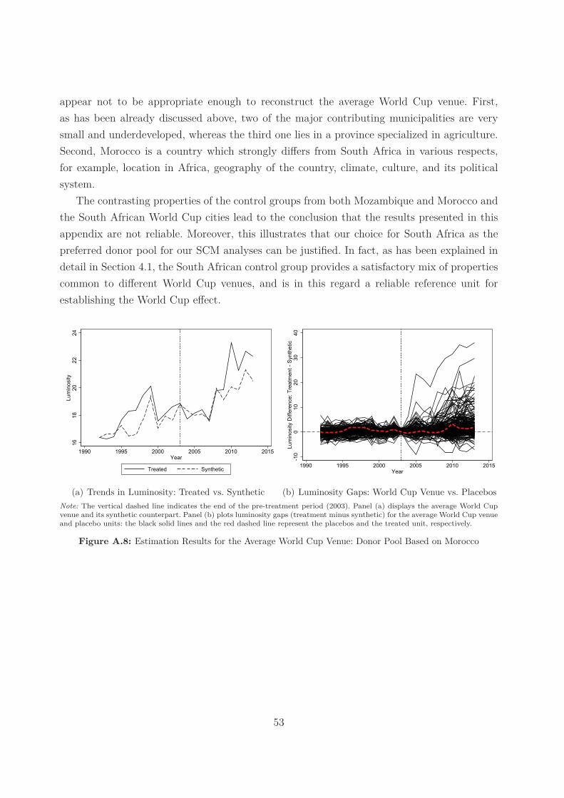
appear not to be appropriate enough to reconstruct the average World Cup venue. First,as has been already discussed above, two of the major contributing municipalities are verysmall and underdeveloped, whereas the third one lies in a province specialized in agriculture.Second, Morocco is a country which strongly differs from South Africa in various respects,for example, location in Africa, geography of the country, climate, culture, and its politicalsystem.

The contrasting properties of the control groups from both Mozambique and Morocco andthe South African World Cup cities lead to the conclusion that the results presented in thisappendix are not reliable. Moreover, this illustrates that our choice for South Africa as thepreferred donor pool for our SCM analyses can be justified. In fact, as has been explained indetail in Section 4.1, the South African control group provides a satisfactory mix of propertiescommon to different World Cup venues, and is in this regard a reliable reference unit forestablishing the World Cup effect.

1618

2022

24Lu

min

osity

1990 1995 2000 2005 2010 2015Year

Treated Synthetic


-10

010

2030

40Lu

min

osity

Diff

eren

ce: T

reat

men

t - S

ynth

etic

1990 1995 2000 2005 2010 2015Year


Figure A.8: Estimation Results for the Average World Cup Venue: Donor Pool Based on Morocco

53

B Data and Setting Details

B.1 Description of Variables

Area. Area of a municipality in square kilometers. Calculated with ArcGIS Pro “CalculateGeometry” tool according to the shapefile of municipality territories from the DIVA-GISdatabase. It can be downloaded at: http://biogeo.ucdavis.edu/data/diva/adm/ZAF_adm.zip (last accessed on January 19, 2106).

Distance to Railway. Geodesic distance from the centroid (mid-point) of each municipalityto the next railway in kilometers. The course of the railways in South Africa is taken froma shapefile provided by the DIVA-GIS database of UC Davies. It can be downloaded at:http://biogeo.ucdavis.edu/data/diva/rrd/ZAF_rrd.zip (last accessed on January 22,2016). The centroids are calculated using the ArcGIS Pro “Calculate Centroids” tool.

Elevation. Elevation data are taken from the NASA SRTM (Shuttle Radar TopographicMission) data set (Version 4.0). The spatial resolution of the data is 3 arc seconds (ap-prox. 90m on the equator). The data is provided by the Consortium for Spatial Informa-tion (CGIAR-CSI). A detailed description can be found at: http://srtm.csi.cgiar.org/and here http://www.cgiar-csi.org/data/srtm-90m-digital-elevation-database-v4-1#introduction. It can be downloaded from this webpage: http://srtm.csi.cgiar.org/SELECTION/inputCoord.asp (last accessed on January 21, 2016).

Share Indigenous People. Share of a municipality’s population with indigenous background.Data come from the project “Spatial Aspects of Unemployment in South Africa 1991–2011”,conducted by the Human Sciences Research Council (HSRC). The data set covers the years1991, 1996, 2001, and 2011. It merges information from the official South African Censusesin 1991, 1996, 2001, and 2011 and the Community Survey in 2007. The geographic units aredefined according to the 2005 municipal boundaries. It can be downloaded (after free reg-istration) at: http://curation.hsrc.ac.za/Dataset-342-datafiles.phtml (last accessedon January 22, 2016).

GDP per capita. GDP per capita (in Rand) on provincial level is calculated based onthe official regional GDP estimates provided by Statistics South Africa (e.g., here http://www.statssa.gov.za/publications/P0441/P04413rdQuarter2009.pdf, last accessed onJanuary 8, 2016). We take GDP estimates in current Rand and deflate them in prices of2005 using annual inflation rates from the website: http://www.inflation.eu/inflation-rates/south-africa/historic-inflation/cpi-inflation-south-africa.aspx (last ac-cessed on January 7, 2016). Finally, to obtain provincial GDP per capita, the deflated

54

GDP is divided by provincial population. Provincial population figures come from theSouth African Census in 2011 (http://www.statssa.gov.za/census/census_2011/census_products/Provinces%20at%20a%20glance%2016%20Nov%202012%20corrected.pdf, last ac-cessed on January 7, 2016).

Income per capita. Income per capita for the year 2007 originates from the HSRC data set“Spatial Aspects of Unemployment in South Africa 1991–2011” (see GDP per capita).

Share Tertiary Education. Share of a municipality’s population with a degree from a universityor another educational institution in the tertiary sector. Data originate from the HSRC dataset “Spatial Aspects of Unemployment in South Africa 1991–2011” (see GDP per capita).

Soil Quality. Data on soil quality are taken from the Zabel et al. (2014) data set. The data set isdescribed further at: http://geoportal-glues.ufz.de/stories/globalsuitability.html(last accessed on January 22, 2016). The measure used in the paper is the average agriculturalsuitability over the period 1961–1990. To measure suitability, Zabel et al. (2014) considerclimate (temperature, precipitation, solar radiation), soil (pH, texture, salinity, organic car-bon content, etc.), and topography (elevation and slope) of an area. They consider rain-fedconditions and irrigation. To construct the suitability measure, they contrast these factorswith growing requirements of 16 plants (Barley, Cassava, Groundnut, Maize, Millet, Oilpalm,Potato, Rapeseed, Rice, Rye, Sorghum, Soy, Sugarcane, Sunflower, Summer wheat, Winterwheat).

Unemployment Rate. Share of a municipality’s work force that is unemployed. Data originatefrom the HSRC data set “Spatial Aspects of Unemployment in South Africa 1991–2011” (seeGDP per capita).

The variables of the ward level data set used in Section 4.2 originate from the same sourcesand are defined analogously to those of the municipality level data set.

B.2 List of Considered Treatments

Table B2.1 reports 72 treatments considered in this paper, i.e., projects that—according to ourinformation—have been directly related to the 2010 World Cup and that we are able to locateusing coordinates given by wikipedia, google maps, and the websites http://www.geonames.org and http://www.mbendi.com.7 In the baseline analysis of the paper, the definition oftreated regions is restricted to nine municipalities comprising a World Cup venue and we thus

7 We only consider information on newly built or refurbished roads if the subject of the project was anational (N) or regional (R) route. All URLs referred to in this Appendix have been last accessed on February12, 2016.

55

consider as treatments those 61 projects out of 72 which have been conducted in World Cupvenues. In one robustness check in Appendix A, we expand the definition of treated regionsto all 16 municipalities that have experienced a World Cup investment, and in this case weuse all 72 treatments. Using the listed treatments, we can identify treated wards within thetreated municipalities.8 Apart from 72 treatments, Table B2.1 also provides information onthe Richards Bay Coal Terminal project, a large investment project unrelated to the WorldCup, that is taken into account in another robustness check in Appendix A.The following list of 73 projects is a part of the large list of 127 projects we identified forSouth Africa for the time span 2004 – 2013 (in which our luminosity data are available).The large list is a result of our own extensive research and can be downloaded at: http://www.martynamarczak.com/research/SA_AllProjects.pdf. Next to the 72 projects fromTable B2.1, that are explicitly related to the 2010 World Cup, the large list also contains 55other investments that

• have been made after the World Cup or

• have been made before/during the World Cup but no direct link with the event ismentioned in the information source, or

• were originally earmarked as World Cup projects but we exclude them from our analysis.

Infrastructure projects related to the 2010 World Cup but excluded in our study are:

• N4 Northern Bypass in Nelspruit, also called Nelspruit Ring Road (Municipality:Mbombela Local, Province: Mpumalanga): this project could not be localized.

• The Khulani Corridor and the Bus Rapid Transit (BRT) System in Port Elizabeth (Mu-nicipality: Nelson Mandela Bay Metropolitan, Province: Eastern Cape)This project has been identified as one of the legacy projects of the World Cup.9 TheKhulani Corridor should provide a link between Motherwell in the northern part of PortElizabeth with the Central Business District (CBD) via an efficient public transport sys-tem, the so–called Bus Rapid Transit (BRT) System, and thus enhance integration of

8 Note that the listed treatments are those for which explicit information could be obtained. We also assumein our study some additional treatments. In particular, we assume that railway stations within each of theWorld Cup municipalities were upgraded even if no specific information about upgrades can be found, e.g., inthe case of the Nelspruit railway station. We also consider the upgrade of the Nelson Mandela MetropolitanUniversity Stadium as a treatment. This stadium was utilized as a training stadium during the World Cup,but, in contrast to the training stadiums included in Table B2.1, we do not dispose of explicit informationabout such an upgrade.

9 http://www.gcis.gov.za/sites/www.gcis.gov.za/files/docs/resourcecentre/multimedia/sa2010_govprep.pdf

56

better developed with less developed areas of the city.10 However, by 2010, only one partof the BRT system could be finalized—a route operated by a shuttle service and runningbetween the CBD and the Nelson Mandela Bay Stadium (also in the city centre).11 Inthe years after the tournament, the implementation of the BRT system has been delayedby different factors, e.g., conflicts with the taxi industry, flawed construction of the fastbus lanes (as a consequence, newly built lanes have been demolished since busses boughtin 2009 could not fit into the lanes), frequently changing city and municipality admin-istration, as well as engineering firms contracted for the BRT project. Only in January2013, a pilot project of the Integrated Public Transport System (IPTS), originally calledthe BRT system, was launched.12 The bus stops of the pilot project were provisionaland new bus stations were at the design stage at that time.13 After the one-year pilotproject, many issues have still not been resolved, like the agreement with the taxi in-dustry14 or flaws in the construction and design.15 Moreover, despite the grant supportby the National Treasury, the municipality has not managed to finance the next projectphases.16 All these developments show that the IPTS in Port Elizabeth was not fullyfunctioning by the end of 2013 (the end of our data sample), so that we decided not totake into account this project in our study.

Total expenditures of all listed World Cup related projects amount to $14 billion and aredisaggregated as follows:

1. $2.5 billion: Stadiums (World Cup stadiums and training stadiums)

2. $11.4 billion: Transport infrastructure

• $3.8 billion: Airports

• $3.6 billion: Rail

• $2.9 billion: Roads

• $1.1 billion: Public transport

3. $88.3 million: Water projects10http://www.nelsonmandelabay.gov.za/datarepository/documents/QDL3C_IDP%20-%20Chapter%

203.pdf11http://www.2010worldcupimpact.info/2010/06/24/fast-bus-lanes-for-port-elizabeth/12http://legacy.nelsonmandelabay.gov.za/Content.aspx?objID=54713http://www.nelsonmandelabay.gov.za/NewsView.aspx?ID=168414Laphum’ilanga (2014, June 2) “Newsflash”, No. 1. Available at: http://laphumilanga.co.za/docs/

Laphumilanga%20newsletter1-2June2014.pdf15http://ewn.co.za/2016/02/03/Multi-million-rand-buses-too-big-for-PE-roads16http://www.heraldlive.co.za/bus-plan-bleeding-money/

57

This figure substantially exceeds the official figure that has been published by Grant Thornton,an independent accounting and consulting firm, whose findings are referred to in reports of theSouth African government; see, for example, the report by Sport and Recreation South Africa(2013). According to Grant Thornton, total expenditures on stadiums and infrastructure di-rectly related to the World Cup were $5.5 billion, with $4.1 spent by the government and $1.4billion spent by cities and provinces.17 A potential explanation for the difference between thefigures provided by Grant Thornton and that corresponding to the treatments in Table B2.1could be the fact that Grant Thornton might have followed a narrow definition of projectsdirectly related to the 2010 World Cup in their calculations. In our study, on the contrary,each project for which we found a link to the World Cup (in any potential information source)counts as World Cup related.

17 See http://mg.co.za/article/2015-06-11-was-world-cup-2010-worth-it.

58

Tab

leB

2.1:

Infr

astr

uctu

rean

dO

ther

Pro

ject

sin

Trea

ted

Mun

icip

alit

ies

Tre

ated

Mun

icip

alit

ya)

Wor

ldC

upV

enue

/Sea

tP

roje

cts

Dur

atio

nC

osts

inU

.S.$

b)So

urce

c)

With

a20

10W

orld

Cup

venu

e

Cit

yof

Joha

nnes

burg

Met

ropo

litan

(Gau

teng

)Jo

hann

esbu

rg

Socc

erC

ity

Stad

ium

2007

–20

0945

1.6

mill

ion

See

note

d)E

llis

Par

kSt

adiu

m20

07–

2009

75,2

69

Tra

inin

gSt

adiu

ms

Orl

ando

Stad

ium

2007

–20

1086

.6m

illio

n

•ht

tp:/

/www

.job

urg-

arch

ive.

co.z

a/20

07/p

dfs/

idp_

2007

/inv

iew/

2010

.pdf

•ht

tp:/

/www

.job

urg-

arch

ive.

co.z

a/20

07/p

dfs/

idp_

2007

/inv

iew/

2010

.pdf

Dob

sonv

ille

Stad

ium

Cec

ilP

ayne

Stad

ium

Rab

ieR

idge

Stad

ium

Ran

dSt

adiu

m

Rui

msi

gSt

adiu

m

Rea

Vay

a(B

usR

apid

Tra

nsit

Syst

em)

2007

–20

09(P

hase

1A)

410.

6m

illio

n(2

06m

illio

n:P

hase

1A)

http

://m

irro

r.un

habi

tat.

org/

down

load

s/do

cs/7

997_

8156

9_Re

a_Va

ya.p

df

Gau

teng

Free

way

Impr

ovem

ent

Pro

ject

(GF

IP)g)

2007

–20

10/2

011

2.7

billi

on(t

otal

for

the

prov

ince

)

Nat

iona

lTre

asur

y:R

epub

licof

Sout

hA

fric

a(2

012)

“Bud

get

Rev

iew

”.A

vaila

ble

at:h

ttp:

//ww

w.tr

easu

ry.

gov.

za/d

ocum

ents

/nat

iona

l%20

budg

et/2

012/

revi

ew/

Gau

trai

ng)

2006

–20

11/2

012

3.4

billi

on(t

otal

for

the

prov

ince

)

http

://w

ww.e

ngin

eeri

ngne

ws.c

o.za

/art

icle

/co

untd

own-

begi

ns-a

s-ga

utra

in-s

team

s-to

ward

s-ju

ne-

dead

line

-201

1-05

-27

Urb

anR

ailw

aySt

atio

ns

Lan

glaa

gte

–20

1045

.7m

illio

nSe

eno

tef)

New

Can

ada

Nas

rec

Orl

ando

Elli

sP

ark

Doo

rnfo

ntei

n

Rho

desfi

eld

59

Tre

ated

Mun

icip

alit

ya)

Wor

ldC

upV

enue

/Sea

tP

roje

ctD

urat

ion

Cos

tsin

U.S

.$b)

Sour

cec)

Reh

abili

tati

onof

Klip

rivi

er/K

lipsp

ruit

2008

–20

1282

.1m

illio

n

•ht

tp:/

/www

.une

p.or

g/PD

F/Pr

essR

elea

ses/

FIFA

_20

10_L

R.pd

f

•ht

tp:/

/www

.jhb

city

park

s.co

m/pd

fs/g

reen

ing_

sowe

to12

.pdf

Cit

yof

Tsh

wan

eM

etro

polit

an(G

aute

ng)

Pre

tori

a

Lof

tus

Ver

sfel

dSt

adiu

m20

07–

2009

12.3

mill

ion

See

note

d);

http

://w

ww.s

outh

afri

ca.n

et/z

a/de

/ar

ticl

es/e

ntry

/art

icle

-sou

thaf

rica

.net

-lof

tus-

vers

feld

-sta

dium

-pre

tori

a

Tra

inin

gSt

adiu

ms

Luc

asM

orip

eSt

adiu

m20

07–

2009

48.3

mill

ion

•ht

tp:/

/www

.iol

.co.

za/n

ews/

sout

h-af

rica

/tsh

wane

-to

-get

-maj

or-u

pgra

des-

for-

2010

-444

853

•C

ounc

ilC

ity

ofT

shw

ane

(200

8)“I

tem

25:

Cog

nisa

nce

ofth

eC

ity’

sP

repa

rati

ons

for

the

2010

FIF

AW

orld

Cup

’sO

vera

llB

usin

ess

Pla

n(P

art

2)”.

Rep

ort

May

29,

2008

.A

vaila

ble

at:

http

://w

ww.t

shwa

ne.g

ov.z

a/si

tes/

Coun

cil/

Coun

cil%

20Re

solu

tion

s

HM

Pit

jeSt

adiu

m

Gia

ntSt

adiu

m

Won

derb

oom

Air

port

–20

0960

.2m

illio

nww

w.so

utha

fric

a.in

fo/b

usin

ess/

econ

omy/

infr

astr

uctu

re/w

onde

rboo

m-02

1109

.htm

Urb

anR

ailw

aySt

atio

ns

Lof

tus

–20

102.

7m

illio

nSe

eno

tef)

Bel

leO

mbr

e

Cit

yof

Cap

eT

own

Met

ropo

litan

(Wes

tern

Cap

e)C

ape

Tow

n

Cap

eT

own

Stad

ium

(new

cons

truc

tion

)20

07–

2009

602.

2m

illio

nSe

eno

ted)

Cap

eT

own

Inte

rnat

iona

lA

irpo

rt–

2010

273.

7m

illio

nww

w.so

utha

fric

a.in

fo/b

usin

ess/

econ

omy/

infr

astr

uctu

re/a

irpo

rts-

0611

09.h

tm

Urb

anR

ailw

aySt

atio

ns

Cap

eT

own

Cen

tury

Stat

ion

(new

cons

truc

tion

)–

2010

7.9

mill

ion

See

note

f)

Cap

eT

own

Stat

ion

–20

10

65.4

mill

ion

See

note

f)

Ath

lone

–20

10ht

tp:/

/www

.met

rora

il.c

o.za

/pdf

/MED

IA-R

ELEA

SE-

PRAS

Area

dy22

0rol

l-Mo

sesM

abhi

daSt

atio

nLau

nch.

pdf

Hei

deve

ld

Lan

ga

60

Tre

ated

Mun

icip

alit

ya)

Wor

ldC

upV

enue

/Sea

tP

roje

ctD

urat

ion

Cos

tsin

U.S

.$b)

Sour

cec)

MyC

iTi(

Bus

Rap

idT

rans

itSy

stem

)20

08–

2013

(Pha

se1A

)62

9.5

mill

ion

(est

imat

edco

sts

2010

)

•ht

tp:/

/myc

iti.

org.

za/d

ocs/

1029

/Hig

hlig

hts_

2010

_My

CiTi

_Bus

ines

s_Pl

an.p

df

•ht

tp:/

/myc

iti.

org.

za/d

ocs/

885/

MyCi

Ti%

20St

akeh

olde

r%20

Guid

e%20

-%20

Janu

ary%

2020

13.p

df

eThe

kwin

iM

etro

polit

an(K

waZ

ulu–

Nat

al)

Dur

ban

Dur

ban

Stad

ium

(new

cons

truc

tion

)20

08–

2009

465.

3m

illio

nSe

eno

ted)

Tra

inin

gSt

adiu

ms

Kin

gZw

elit

hini

Stad

ium

2007

–20

1034

.2m

illio

nht

tp:/

/www

.eng

inee

ring

news

.co.

za/p

rint

-ver

sion

/st

adiu

ms-2

009-

10-0

2P

rinc

ess

Mag

ogo

Stad

ium

Suga

rR

ayX

ulu

Stad

ium

Kin

gSh

aka

Inte

rnat

iona

lA

irpo

rt20

07–

2010

930.

6m

illio

nSe

eno

tee)

;ht

tp:/

/www

.eng

inee

ring

news

.co.

za/

arti

cle/

cons

truc

tion

-tak

es-o

ff-a

t-ne

w-du

rban

-ai

rpor

t-de

spit

e-le

gal-

chal

leng

e-20

07-0

9-14

Urb

anR

ailw

aySt

atio

ns

Dur

ban

Mos

esM

abhi

daSt

atio

n(n

ewco

nstr

ucti

on)

–20

1020

.5m

illio

nSe

eno

tef)

Dur

ban

Kw

a-M

nyan

du–

2010

7.7

mill

ion

See

note

f)D

urba

nK

waM

ashu

Reu

nion

N2

Dub

eT

rade

Por

tIn

terc

hang

e20

08–

2010

41.6

mill

ion

•SA

NR

AL

(201

1)“A

nnua

lRep

ort”

.Ava

ilabl

eat

:ht

tp:/

/www

.nra

.co.

za/c

onte

nt/S

ANRA

L_An

nual

_Re

port

2011

.pdf

•ht

tp:/

/www

.wbh

o.co

.za/

n2-i

nter

chan

ge/

•“K

ing

Shak

aIn

tern

atio

nalA

irpo

rtN

2In

terc

hang

e”(2

011,

Dec

embe

r).C

ivil

Eng

inee

ring

.Ava

ilabl

eat

:ht

tp:/

/www

.civ

ilde

sign

er.c

om/P

ubli

cati

ons/

king

shak

an2.

pdf

61

Tre

ated

Mun

icip

alit

ya)

Wor

ldC

upV

enue

/Sea

tP

roje

ctD

urat

ion

Cos

tsin

U.S

.$b)

Sour

cec)

Nel

son

Man

dela

Bay

Met

ropo

litan

(Eas

tern

Cap

e)

Por

tE

lizab

eth

Nel

son

Man

dela

Bay

Stad

ium

(new

cons

truc

tion

)20

07–

2009

280.

5m

illio

nSe

eno

ted)

Gel

vend

ale

Stad

ium

(tra

inin

gst

adiu

m)

2007

–20

1011

.2m

illio

nht

tp:/

/www

.sbt

buil

ding

.co.

za/#

/!pr

ojec

ts

Por

tE

lizab

eth

Air

port

–20

089.

4m

illio

nA

CSA

(200

9)“A

nnua

lRep

ort

Par

tII

I”.A

vaila

ble

at:

http

://w

ww.a

irpo

rts.

co.z

a/Pa

ges/

Fina

ncia

lInf

orma

tion

.asp

x

Nor

thE

ndR

ailw

aySt

atio

n–

2010

2.2

mill

ion

See

note

f)

Man

gaun

gM

etro

polit

an(F

ree

Stat

e)B

loem

font

ein

Free

Stat

eSt

adiu

m20

07–

2009

48m

illio

nSe

eno

ted)

;ht

tps:

//pm

g.or

g.za

/com

mitt

ee-m

eeti

ng/1

1852

/

Seis

aR

amab

odu

Stad

ium

(tra

inin

gst

adiu

m)

—1.

4m

illio

nht

tp:/

/www

.iol

.co.

za/s

port

/fre

e-st

ate-

stad

ium-

to-

open

-on-

apri

l-4-

6001

26

Blo

emfo

ntei

nA

irpo

rt20

07–

2009

23.3

mill

ion

See

note

e);

http

://w

ww.e

ngin

eeri

ngne

ws.c

o.za

/art

icle

/air

port

-up

grad

es-o

n-tr

ack-

ahea

d-of

-201

0-20

07-1

2-14

N8:

Blo

emfo

ntei

nA

irpo

rtIn

terc

hang

e(a

ndac

cess

road

s)20

09–

2010

17.4

mill

ion

•SA

NR

AL

(200

9)“A

nnua

lRep

ort”

.Ava

ilabl

eat

:ht

tp:/

/www

.nra

.co.

za/c

onte

nt/S

anra

l_AR

_09.

pdf

•ht

tp:/

/www

.eng

inee

ring

news

.co.

za/p

rint

-ve

rsio

n/co

nsul

tant

s-to

-com

plet

e-fr

eewa

y-im

prov

emen

t-ah

ead-

of-s

ched

ule-

2010

-10-

08

Man

gaun

gIn

term

odal

Tra

nspo

rtC

entr

e20

09–

2010

54.7

mill

ion

•ht

tp:/

/www

.sme

c.co

m/De

faul

t.as

px?a

Proj

Id=9

15

•ht

tp:/

/tru

spac

e.wi

x.co

m/ho

me#!

proj

ect-

mitf

/gfw

b5

Mbo

mbe

laL

ocal

(Mpu

mal

anga

)N

elsp

ruit

Mbo

mbe

laSt

adiu

m(n

ewco

nstr

ucti

on)

2007

–20

0914

3.7

mill

ion

See

note

d)

Mat

affin

Wat

erR

eser

voir

2008

–20

106.

2m

illio

n

Nat

iona

lTre

asur

y:R

epub

licof

Sout

hA

fric

a(2

011)

“Est

imat

esof

Nat

iona

lExp

endi

ture

:Wat

erA

ffair

s”.

Ava

ilabl

eat

:htt

p://

www.

trea

sury

.gov

.za/

docu

ment

s/na

tion

al%2

0bud

get/

2011

/ene

book

lets

/

Pol

okw

ane

Loc

al(L

impo

po)

Pol

okw

ane

Pet

erM

okab

aSt

adiu

m(n

ewco

nstr

ucti

on)

2007

–20

0916

9.7

mill

ion

See

note

d)

Pol

okw

ane

Air

port

2008

10.4

mill

ion

(joi

ntw

ith

cost

for

Giy

ania

ndT

hoho

yand

ouA

irpo

rts)

http

://w

ww.g

cis.

gov.

za/s

ites

/def

ault

/fil

es/d

ocs/

reso

urce

cent

re/y

earb

ook/

2008

/cha

pter

1.pd

f

62

Tre

ated

Mun

icip

alit

ya)

Wor

ldC

upV

enue

/Sea

tP

roje

ctD

urat

ion

Cos

tsin

U.S

.$b)

Sour

cec)

Pol

okw

ane

Eas

tern

Rin

gR

oad

2009

–20

1111

8.4

mill

ion

•ht

tp:/

/kbk

engi

neer

s.co

.za/

proj

ect-

port

foli

o/tr

ansp

orta

tion

/

•ht

tp:/

/www

.nra

.co.

za/l

ive/

cont

ent.

php?

Sess

ion_

ID=a

1117

23f2

33d6

7e2b

636a

05ef

c5bc

988&

Cate

gory

_ID

=159

•SA

NR

AL

(201

0)“A

nnua

lRep

ort”

.Ava

ilabl

eat

:htt

p://

www.

nra.

co.z

a/co

nten

t/Sa

nral

_ARe

p_10

_Web

.pdf

Rus

tenb

urg

Loc

al(N

orth

Wes

t)R

uste

nbur

gR

oyal

Bak

ofen

gSt

adiu

m20

07–

2009

49.3

mill

ion

See

note

d);

http

://w

ww.s

outh

afri

ca.n

et/z

a/de

/ar

ticl

es/e

ntry

/art

icle

-sou

thaf

rica

.net

-roy

al-

bafo

keng

-sta

dium

-rus

tenb

urg

Oly

mpi

aP

ark

Stad

ium

(tra

inin

gst

adiu

m)

——

HSR

C(2

011)

“FIF

A20

10W

orld

Cup

Leg

acy

Aud

it”.

Ava

ilabl

eat

:htt

p://

www.

hsrc

.ac.

za/e

n/re

sear

ch-

outp

uts/

view

/563

6

Rus

tenb

urg

Rai

lway

Stat

ion

–20

10—

HSR

C(2

011)

“FIF

A20

10W

orld

Cup

Leg

acy

Aud

it”.

Ava

ilabl

eat

:htt

p://

www.

hsrc

.ac.

za/e

n/re

sear

ch-

outp

uts/

view

/563

6

Oth

erm

unic

ipal

ities

Eku

rhul

eni

Met

ropo

litan

(Gau

teng

)G

erm

isto

nO

.R.T

ambo

Inte

rnat

iona

lA

irpo

rt–

2009

2.4

billi

on(t

otal

esti

mat

edco

sts)

http

://w

ww.a

irpo

rtsi

nter

nati

onal

.com

/201

0/05

/wo

rld-

cup-

airp

orts

/553

8

Buff

alo

Cit

yM

etro

polit

an(E

aste

rnC

ape)

Eas

tL

ondo

n

Tra

inin

gSt

adiu

ms

Buff

alo

Cit

ySt

adiu

m20

08–

2010

3.7

mill

ion

HSR

C(2

011)

“FIF

A20

10W

orld

Cup

Leg

acy

Au-

dit”

.A

vaila

ble

at:

http

://w

ww.h

src.

ac.z

a/en

/res

earc

h-ou

tput

s/vi

ew/5

636

Bhi

sho

Stad

ium

Eas

tL

ondo

nA

irpo

rt–

2010

13.7

mill

ion

www.

sout

hafr

ica.

info

/new

s/bu

sine

ss/4

9272

4.ht

m

Bhi

sho

Air

port

2007

–20

0810

.7m

illio

n

•ht

tp:/

/www

.sou

thaf

rica

.inf

o/bu

sine

ss/i

nves

ting

/op

port

unit

ies/

ecai

rpor

t-02

0807

.htm

•ht

tp:/

/www

.eng

inee

ring

news

.co.

za/p

rint

-ve

rsio

n/ea

ster

n-ca

pe-t

o-co

mple

te-m

that

ha-

airp

ort-

upgr

ade-

befo

re-w

orld

-cup

-200

9-12

-04

63

Tre

ated

Mun

icip

alit

ya)

Wor

ldC

upV

enue

/Sea

tP

roje

ctD

urat

ion

Cos

tsin

U.S

.$b)

Sour

cec)

Kin

gSa

bata

Dal

indy

ebo

(Eas

tern

Cap

e)M

that

haM

that

haA

irpo

rt20

09–

2015

(wit

hde

lays

)95

.8m

illio

n

•ht

tp:/

/www

.eng

inee

ring

news

.co.

za/p

rint

-ver

sion

/mt

hath

a-ai

rpor

t-up

grad

e-so

uth-

afri

ca-2

010-

03-0

5

•ht

tp:/

/www

.gov

.za/

mtha

tha-

airp

ort-

upgr

ade-

back

-tr

ack

•ht

tp:/

/www

.ksd

.gov

.za/

comp

onen

t/k2

/ite

mlis

t/ta

g/Mt

hath

aAir

port

Mth

atha

Stad

ium

(tra

inin

gst

adiu

m;n

ewco

nstr

ucti

on)

2008

–20

1030

mill

ion

HSR

C(2

011)

“FIF

A20

10W

orld

Cup

Leg

acy

Aud

it”.

Ava

ilabl

eat

:htt

p://

www.

hsrc

.ac.

za/e

n/re

sear

ch-

outp

uts/

view

/563

6

Geo

rge

Loc

al(W

este

rnC

ape)

Geo

rge

Geo

rge

Air

port

2004

–20

075.

9m

illio

nht

tp:/

/www

.eng

inee

ring

news

.co.

za/a

rtic

le/g

eorg

e-ai

rpor

t-re

ceiv

es-r

43mi

llio

n-up

grad

e-20

07-1

2-14

SolP

laat

jeL

ocal

(Nor

ther

nC

ape)

Kim

berl

eyK

imbe

rley

Air

port

–20

102.

3m

illio

n

•A

CSA

(201

0)“A

nnua

lRep

ort

2010

Par

tII

I”.

Ava

ilabl

eat

:htt

p://

www.

airp

orts

.co.

za/

Fina

ncia

lRes

ults

/Ann

ualR

epor

tpar

tIII

2010

.pdf

•Se

eno

tee)

//K

hara

Hai

sL

ocal

(Nor

ther

nC

ape)

Upi

ngto

nU

ping

ton

Air

port

–20

104.

2m

illio

n

•A

CSA

(201

0)“A

nnua

lRep

ort

2010

Par

tII

I”.

Ava

ilabl

eat

:htt

p://

www.

airp

orts

.co.

za/

Fina

ncia

lRes

ults

/Ann

ualR

epor

tpar

tIII

2010

.pdf

•Se

eno

tee)

Ngw

athe

Loc

al(F

ree

Stat

e)P

arys

Fezi

leD

abiS

tadi

um(t

rain

ing

stad

ium

)20

08–

2012

7.9

mill

ion

Nat

iona

lTre

asur

ySo

uth

Afr

ica

(201

1).“

Pro

vinc

ial

Bud

get

Free

Stat

e:V

ote

12(S

port

s,A

rts,

Cul

ture

and

Rec

reat

ion)

”.A

vaila

ble

at:

http

://w

ww.t

reas

ury.

gov.

za/d

ocum

ents

/pro

vinc

ial%

20bu

dget

/201

1/Bu

dget

%20S

tate

ment

s/FS

/

Oth

erm

unic

ipal

ities

:pr

ojec

tsun

rela

ted

toth

e20

10W

orld

Cup

uMhl

athu

zeL

ocal

(Kw

aZul

u–N

atal

)R

icha

rds

Bay

Ric

hard

sB

ayC

oalT

erm

inal

(Pha

se5)

2006

–20

1016

4.2

mill

ion

•ht

tp:/

/www

.rbc

t.co

.za/

abou

t-rb

ct-4

/our

-his

tory

/

•ht

tp:/

/www

.eng

inee

ring

news

.co.

za/a

rtic

le/

rich

ards

-bay

-coa

l-te

rmin

al-e

xpan

sion

-and

-coa

l-li

ne-s

outh

-afr

ica-

2009

-02-

06

a)T

heco

rres

pond

ing

prov

ince

isgi

ven

inbr

acke

ts.

b)A

llfig

ures

orig

inal

lygi

ven

inth

ena

tion

alcu

rren

cy‘R

and’

have

been

tran

slat

edin

toU

.S.d

olla

rs($

)us

ing

the

aver

age

exch

ange

rate

of20

10.

c)T

heU

RL

sha

vebe

enla

stac

cess

edon

Febr

uary

12,2

016.

d)ht

tp:/

/www

.med

iacl

ubso

utha

fric

a.co

m/co

mpon

ent/

cont

ent/

arti

cle?

id=9

3:wo

rld

e)ht

tp:/

/www

.air

port

-bus

ines

s.co

m/20

10/0

3/ac

sas-

airp

ort-

deve

lopm

ents

-nea

ring

-con

clus

ion-

as-w

orld

-cup

-app

roac

hes/

f)ht

tp:/

/www

.met

rora

il.c

o.za

/pdf

/Orl

ando

Stat

ionL

aunc

h.pd

fg)

Thi

spr

ojec

tal

soap

plie

sto

the

Cit

yof

Tsh

wan

eM

etro

polit

anM

unic

ipal

ity.

64

C Additional Tables and Figures

C.1 Tables

Table C1.1: Descriptive Overview of the Muncipality Level Data Set

Variable Obs. Mean Std. Dev. Min. Max.

Luminosity 5,192 3.117 6.432 0 58.107

Area 5,192 5,203.189 5,395.449 251.434 36,127.950

Distance to Railway 5,192 2.045 6.854 0 44.842

Elevation 5,192 986.556 477.231 53.303 1,922.893

GDP per capita 702 26,896.73 9,828.787 12,986.54 56,768.83

Income per capita 237 15,781.66 11,986.76 1,113.61 82,477.9

Share Indigenous People 472 0.008 0.024 0 0.206

Share Tertiary Education 708 0.02 0.019 0 0.125

Soil Quality 5,192 36.214 13.419 0.023 64.255

Unemployment Rate 944 33.714 16.356 6.100 84.07

Table C1.2: Average World Cup Venue: Means of Economic Predictors (Pre-Treatment)

Predictor Actual Synthetic

Luminosity 18.8757 18.74631

Area 3722.812 1111.97

Distance to Railway 0 0

Elevation 907.6775 332.8766

Share Indigenous People 0.033037 0.0330786

Share Tertiary Education 0.0660153 0.057515

Soil Quality 39.97758 49.94023

Unemployment Rate 37.65556 40.74773

Note: Means for all economics predictors over the pre-treatmentperiod (1992-2003). Predictors are explained in Section 2 and Ap-pendix B.

65

Table C1.3: Descriptive Overview of Ward Level Data Set for eThekwini


Luminosity 2,266 47.251 17.103 2.332 63

Area 2,266 22.152 30.801 0.905 168.133

Distance to Railway 2,266 1.654 2.108 0 8.062

Elevation 2,266 185.676 157.428 9.296 676.806

Soil Quality 2,266 39.667 9.005 25 66

Table C1.4: Descriptive Overview of Ward Level Data Set for Polokwane


Luminosity 836 20.593 19.271 0.03 63

Area 836 99.105 213.076 2.59 1326.646

Distance to Railway 836 8.374 7.278 0 22.404

Elevation 836 1288.364 59.155 1181.695 1441.94

Soil Quality 836 54.817 5.921 33.261 61.892

Table C1.5: Descriptive Overview of Ward Level Data Set for Rustenburg


Luminosity 836 31.397 19.675 0.799 63

Area 836 90.086 183.592 0.872 1077.936

Distance to Railway 836 1.848 2.710 0 12.178

Elevation 836 1158.558 89.271 1034.207 1480.51

Soil Quality 836 53.665 3.965 40.033 59

66

C.2 Figures

6010

014

018

0Lu

min

osity

1992 1996 2000 2004 2008 2012

Port Elizabeth Johannesburg PretoriaDurban Cape Town BloemfonteinPolokwane Nelspruit Rustenburg

Note: The figure shows the temporal evolution of luminosity between 1992 and 2013 for each of the World Cup venues. Luminosityvalues are indexed with each municipality’s value in 2004 being equal to 100.

Figure C2.1: Mean Luminosity per World Cup Venue, 1992–2013

(a) Distribution of Luminosity in 2003 (b) Distribution of Luminosity in 2013Note: Panel (a) displays pixel level luminosity within the eThekwini Metropolitan Municipality in the last pre-treatment year(2003). Panel (b) displays pixel level luminosity within the eThekwini Metropolitan Municipality in the last post-treatment year(2013). In both panels, the borders of the eThekwini Metropolitan Municipality are depicted in bold-type red, the wards withinthe municipality are colored in light-blue, and the treated wards are shown in bold-type light-green.

Figure C2.2: Pre- and Post-Treatment Pixel Level Distribution of Luminosity in eThekwini

67

5456

5860

6264

Lum

inos

ity

1990 1995 2000 2005 2010 2015Year

Treated Synthetic

Note: The graphic displays the average World Cup venue and its synthetic counterpart.

Figure C2.3: Estimation Results for Cape Town Airport: Trends in Luminosity—Treated vs. Synthetic

(a) Distribution of Luminosity in 2003 (b) Distribution of Luminosity in 2013Note: Panel (a) displays pixel level luminosity within the Polokwane Local Municipality in the last pre-treatment year (2003).Panel (b) displays pixel level luminosity within the Polokwane Local Municipality in the last post-treatment year (2013). In bothpanels, the borders of the Polokwane Local Municipality are depicted in bold-type red, the wards within the municipality arecolored in light-blue, and the treated wards are shown in bold-type light-green.

Figure C2.4: Pre- and Post-Treatment Pixel Level Distribution of Luminosity in Polokwane

68

(a) Distribution of Luminosity in 2003 (b) Distribution of Luminosity in 2013Note: Panel (a) displays pixel level luminosity within the Rustenburg Local Municipality in the last pre-treatment year (2003).Panel (b) displays pixel level luminosity within the Rustenburg Metropolitan Municipality in the last post-treatment year (2013).In both panels, the borders of the Rustenburg Metropolitan Municipality are depicted in bold-type red, the wards within themunicipality are colored in light-blue, and the treated wards are shown in bold-type light-green.

Figure C2.5: Pre- and Post-Treatment Pixel Level Distribution of Luminosity in Rustenburg

4550

5560

65Lu

min

osity

1990 1995 2000 2005 2010 2015Year

Treated Synthetic


-20

-10

010

20Lu

min

osity

Diff

eren

ce: T

reat

men

t - S

ynth

etic

1990 1995 2000 2005 2010 2015Year

(b) Luminosity Gaps: Stadium Ward vs. PlacebosNote: The vertical dashed line indicates the end of the pre-treatment period (2003). Panel (a) displays the stadium ward and itssynthetic counterpart. Panel (b) plots luminosity gaps (treatment minus synthetic) for the stadium ward and placebo units: theblack solid lines and the red dashed line represent the placebos and the treated unit, respectively.

Figure C2.6: Estimation Results: Soccer City Stadium Johannesburg

69

Hohenheim Discussion Papers in Business, Economics and Social Sciences The Faculty of Business, Economics and Social Sciences continues since 2015 the established “FZID Discussion Paper Series” of the “Centre for Research on Innovation and Services (FZID)” under the name “Hohenheim Discussion Papers in Business, Economics and Social Sciences”. Institutes 510 Institute of Financial Management 520 Institute of Economics 530 Institute of Health Care & Public Management 540 Institute of Communication Science 550 Institute of Law and Social Sciences 560 Institute of Economic and Business Education 570 Institute of Marketing & Management 580 Institute of Interorganisational Management & Performance Download Hohenheim Discussion Papers in Business, Economics and Social Sciences from our homepage: https://wiso.uni-hohenheim.de/papers Nr. Autor Titel Inst. 01-2015 Thomas Beissinger,

Philipp Baudy THE IMPACT OF TEMPORARY AGENCY WORK ON TRADE UNION WAGE SETTING: A Theoretical Analysis

520

02-2015 Fabian Wahl

PARTICIPATIVE POLITICAL INSTITUTIONS AND CITY DEVELOPMENT 800-1800

520

03-2015 Tommaso Proietti, Martyna Marczak, Gianluigi Mazzi

EUROMIND-D: A DENSITY ESTIMATE OF MONTHLY GROSS DOMESTIC PRODUCT FOR THE EURO AREA

520

04-2015 Thomas Beissinger, Nathalie Chusseau, Joël Hellier

OFFSHORING AND LABOUR MARKET REFORMS: MODELLING THE GERMAN EXPERIENCE

520

05-2015 Matthias Mueller, Kristina Bogner, Tobias Buchmann, Muhamed Kudic

SIMULATING KNOWLEDGE DIFFUSION IN FOUR STRUCTURALLY DISTINCT NETWORKS – AN AGENT-BASED SIMULATION MODEL

520

06-2015 Martyna Marczak, Thomas Beissinger

BIDIRECTIONAL RELATIONSHIP BETWEEN INVESTOR SENTIMENT AND EXCESS RETURNS: NEW EVIDENCE FROM THE WAVELET PERSPECTIVE

520

07-2015 Peng Nie, Galit Nimrod, Alfonso Sousa-Poza

INTERNET USE AND SUBJECTIVE WELL-BEING IN CHINA

530

08-2015 Fabian Wahl

THE LONG SHADOW OF HISTORY ROMAN LEGACY AND ECONOMIC DEVELOPMENT – EVIDENCE FROM THE GERMAN LIMES

520

09-2015 Peng Nie, Alfonso Sousa-Poza

COMMUTE TIME AND SUBJECTIVE WELL-BEING IN URBAN CHINA

530

Nr. Autor Titel Inst. 10-2015 Kristina Bogner

THE EFFECT OF PROJECT FUNDING ON INNOVATIVE PERFORMANCE AN AGENT-BASED SIMULATION MODEL

520

11-2015 Bogang Jun, Tai-Yoo Kim

A NEO-SCHUMPETERIAN PERSPECTIVE ON THE ANALYTICAL MACROECONOMIC FRAMEWORK: THE EXPANDED REPRODUCTION SYSTEM

520

12-2015 Volker Grossmann Aderonke Osikominu Marius Osterfeld

ARE SOCIOCULTURAL FACTORS IMPORTANT FOR STUDYING A SCIENCE UNIVERSITY MAJOR?

520

13-2015 Martyna Marczak Tommaso Proietti Stefano Grassi

A DATA–CLEANING AUGMENTED KALMAN FILTER FOR ROBUST ESTIMATION OF STATE SPACE MODELS

520

14-2015 Carolina Castagnetti Luisa Rosti Marina Töpfer

THE REVERSAL OF THE GENDER PAY GAP AMONG PUBLIC-CONTEST SELECTED YOUNG EMPLOYEES

520

15-2015 Alexander Opitz DEMOCRATIC PROSPECTS IN IMPERIAL RUSSIA: THE REVOLUTION OF 1905 AND THE POLITICAL STOCK MARKET

520

01-2016 Michael Ahlheim, Jan Neidhardt

NON-TRADING BEHAVIOUR IN CHOICE EXPERIMENTS

520

02-2016 Bogang Jun, Alexander Gerybadze, Tai-Yoo Kim

THE LEGACY OF FRIEDRICH LIST: THE EXPANSIVE REPRODUCTION SYSTEM AND THE KOREAN HISTORY OF INDUSTRIALIZATION

520


FOOD INSECURITY AMONG OLDER EUROPEANS: EVIDENCE FROM THE SURVEY OF HEALTH, AGEING, AND RETIREMENT IN EUROPE

530

04-2016 Peter Spahn POPULATION GROWTH, SAVING, INTEREST RATES AND STAGNATION. DISCUSSING THE EGGERTSSON-MEHROTRA-MODEL

520

05-2016 Vincent Dekker, Kristina Strohmaier, Nicole Bosch

A DATA-DRIVEN PROCEDURE TO DETERMINE THE BUNCHING WINDOW – AN APPLICATION TO THE NETHERLANDS

520

06-2016 Philipp Baudy, Dario Cords

DEREGULATION OF TEMPORARY AGENCY EMPLOYMENT IN A UNIONIZED ECONOMY: DOES THIS REALLY LEAD TO A SUBSTITUTION OF REGULAR EMPLOYMENT?

520

07-2016 Robin Jessen, Davud Rostam-Afschar, Sebastian Schmitz

HOW IMPORTANT IS PRECAUTIONARY LABOR SUPPLY?

520

08-2016 Peng Nie, Alfonso Sousa-Poza, Jianhong Xue

FUEL FOR LIFE: DOMESTIC COOKING FUELS AND WOMEN’S HEALTH IN RURAL CHINA

530

Nr. Autor Titel Inst. 09-2016 Bogang Jun,

Seung Kyu-Yi, Tobias Buchmann, Matthias Müller

THE CO-EVOLUTION OF INNOVATION NETWORKS: COLLABORATION BETWEEN WEST AND EAST GERMANY FROM 1972 TO 2014

520

10-2016 Vladan Ivanovic, Vadim Kufenko, Boris Begovic Nenad Stanisic, Vincent Geloso

CONTINUITY UNDER A DIFFERENT NAME. THE OUTCOME OF PRIVATISATION IN SERBIA

520

11-2016 David E. Bloom Michael Kuhn Klaus Prettner

THE CONTRIBUTION OF FEMALE HEALTH TO ECONOMIC DEVELOPMENT

520

12-2016 Franz X. Hof Klaus Prettner

THE QUEST FOR STATUS AND R&D-BASED GROWTH 520

13-2016 Jung-In Yeon Andreas Pyka Tai-Yoo Kim

STRUCTURAL SHIFT AND INCREASING VARIETY IN KOREA, 1960–2010: EMPIRICAL EVIDENCE OF THE ECONOMIC DEVELOPMENT MODEL BY THE CREATION OF NEW SECTORS

520

14-2016 Benjamin Fuchs THE EFFECT OF TEENAGE EMPLOYMENT ON CHARACTER SKILLS, EXPECTATIONS AND OCCUPATIONAL CHOICE STRATEGIES

520

15-2016 Seung-Kyu Yi Bogang Jun

HAS THE GERMAN REUNIFICATION STRENGTHENED GERMANY’S NATIONAL INNOVATION SYSTEM? TRIPLE HELIX DYNAMICS OF GERMANY’S INNOVATION SYSTEM

520

16-2016 Gregor Pfeifer Fabian Wahl Martyna Marczak

ILLUMINATING THE WORLD CUP EFFECT: NIGHT LIGHTS EVIDENCE FROM SOUTH AFRICA

520

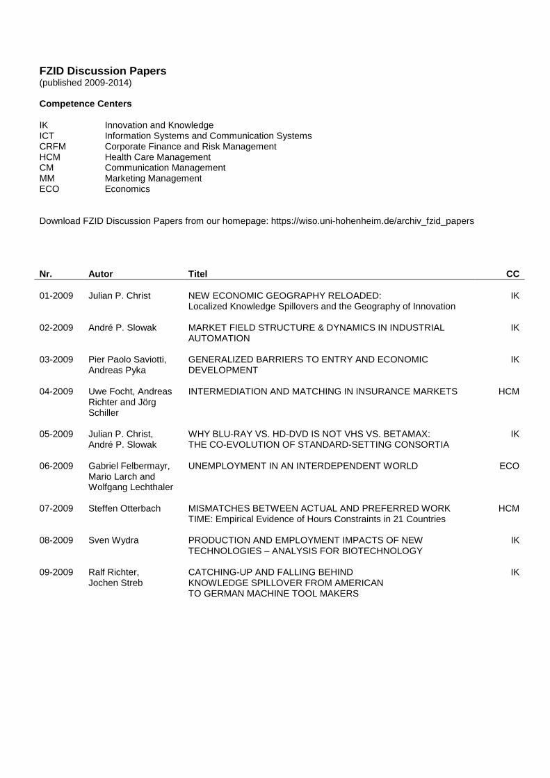
FZID Discussion Papers (published 2009-2014) Competence Centers IK Innovation and Knowledge ICT Information Systems and Communication Systems CRFM Corporate Finance and Risk Management HCM Health Care Management CM Communication Management MM Marketing Management ECO Economics Download FZID Discussion Papers from our homepage: https://wiso.uni-hohenheim.de/archiv_fzid_papers Nr. Autor Titel CC 01-2009

Julian P. Christ

NEW ECONOMIC GEOGRAPHY RELOADED: Localized Knowledge Spillovers and the Geography of Innovation

IK

02-2009 André P. Slowak MARKET FIELD STRUCTURE & DYNAMICS IN INDUSTRIAL AUTOMATION

IK

03-2009 Pier Paolo Saviotti, Andreas Pyka

GENERALIZED BARRIERS TO ENTRY AND ECONOMIC DEVELOPMENT

IK

04-2009 Uwe Focht, Andreas Richter and Jörg Schiller

INTERMEDIATION AND MATCHING IN INSURANCE MARKETS HCM

05-2009 Julian P. Christ, André P. Slowak

WHY BLU-RAY VS. HD-DVD IS NOT VHS VS. BETAMAX: THE CO-EVOLUTION OF STANDARD-SETTING CONSORTIA

IK

06-2009 Gabriel Felbermayr, Mario Larch and Wolfgang Lechthaler

UNEMPLOYMENT IN AN INTERDEPENDENT WORLD ECO

07-2009 Steffen Otterbach MISMATCHES BETWEEN ACTUAL AND PREFERRED WORK TIME: Empirical Evidence of Hours Constraints in 21 Countries

HCM

08-2009 Sven Wydra PRODUCTION AND EMPLOYMENT IMPACTS OF NEW TECHNOLOGIES – ANALYSIS FOR BIOTECHNOLOGY

IK

09-2009 Ralf Richter, Jochen Streb

CATCHING-UP AND FALLING BEHIND KNOWLEDGE SPILLOVER FROM AMERICAN TO GERMAN MACHINE TOOL MAKERS

IK

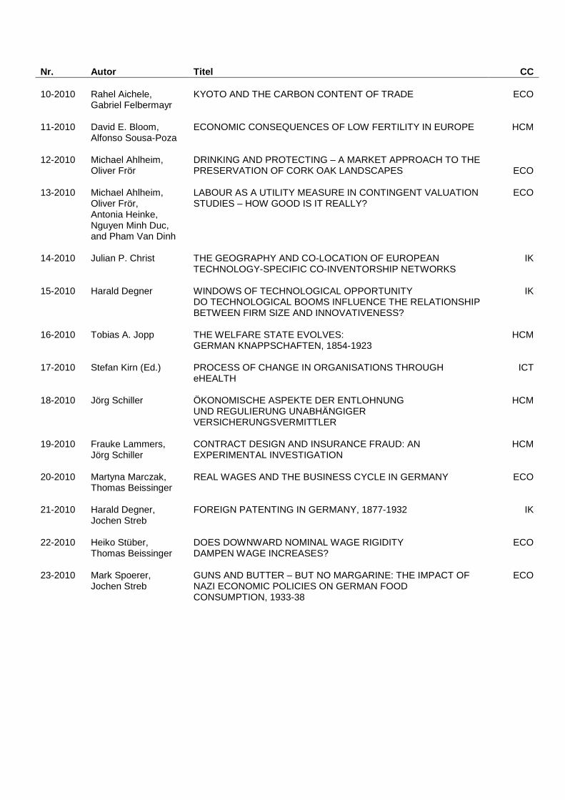
Nr. Autor Titel CC 10-2010

Rahel Aichele, Gabriel Felbermayr

KYOTO AND THE CARBON CONTENT OF TRADE

ECO

11-2010 David E. Bloom, Alfonso Sousa-Poza

ECONOMIC CONSEQUENCES OF LOW FERTILITY IN EUROPE

HCM

12-2010 Michael Ahlheim, Oliver Frör

DRINKING AND PROTECTING – A MARKET APPROACH TO THE PRESERVATION OF CORK OAK LANDSCAPES

ECO

13-2010 Michael Ahlheim, Oliver Frör, Antonia Heinke, Nguyen Minh Duc, and Pham Van Dinh

LABOUR AS A UTILITY MEASURE IN CONTINGENT VALUATION STUDIES – HOW GOOD IS IT REALLY?

ECO

14-2010 Julian P. Christ THE GEOGRAPHY AND CO-LOCATION OF EUROPEAN TECHNOLOGY-SPECIFIC CO-INVENTORSHIP NETWORKS

IK

15-2010 Harald Degner WINDOWS OF TECHNOLOGICAL OPPORTUNITY DO TECHNOLOGICAL BOOMS INFLUENCE THE RELATIONSHIP BETWEEN FIRM SIZE AND INNOVATIVENESS?

IK

16-2010 Tobias A. Jopp THE WELFARE STATE EVOLVES: GERMAN KNAPPSCHAFTEN, 1854-1923

HCM

17-2010 Stefan Kirn (Ed.) PROCESS OF CHANGE IN ORGANISATIONS THROUGH eHEALTH

ICT

18-2010 Jörg Schiller ÖKONOMISCHE ASPEKTE DER ENTLOHNUNG UND REGULIERUNG UNABHÄNGIGER VERSICHERUNGSVERMITTLER

HCM

19-2010 Frauke Lammers, Jörg Schiller

CONTRACT DESIGN AND INSURANCE FRAUD: AN EXPERIMENTAL INVESTIGATION

HCM

20-2010 Martyna Marczak, Thomas Beissinger

REAL WAGES AND THE BUSINESS CYCLE IN GERMANY

ECO

21-2010 Harald Degner, Jochen Streb

FOREIGN PATENTING IN GERMANY, 1877-1932

IK

22-2010 Heiko Stüber, Thomas Beissinger

DOES DOWNWARD NOMINAL WAGE RIGIDITY DAMPEN WAGE INCREASES?

ECO

23-2010 Mark Spoerer, Jochen Streb

GUNS AND BUTTER – BUT NO MARGARINE: THE IMPACT OF NAZI ECONOMIC POLICIES ON GERMAN FOOD CONSUMPTION, 1933-38

ECO


Dhammika Dharmapala, Nadine Riedel

EARNINGS SHOCKS AND TAX-MOTIVATED INCOME-SHIFTING: EVIDENCE FROM EUROPEAN MULTINATIONALS

ECO

25-2011 Michael Schuele, Stefan Kirn

QUALITATIVES, RÄUMLICHES SCHLIEßEN ZUR KOLLISIONSERKENNUNG UND KOLLISIONSVERMEIDUNG AUTONOMER BDI-AGENTEN

ICT

26-2011 Marcus Müller, Guillaume Stern, Ansger Jacob and Stefan Kirn

VERHALTENSMODELLE FÜR SOFTWAREAGENTEN IM PUBLIC GOODS GAME

ICT

27-2011 Monnet Benoit, Patrick Gbakoua and Alfonso Sousa-Poza

ENGEL CURVES, SPATIAL VARIATION IN PRICES AND DEMAND FOR COMMODITIES IN CÔTE D’IVOIRE

ECO

28-2011 Nadine Riedel, Hannah Schildberg-Hörisch

ASYMMETRIC OBLIGATIONS

ECO

29-2011 Nicole Waidlein

CAUSES OF PERSISTENT PRODUCTIVITY DIFFERENCES IN THE WEST GERMAN STATES IN THE PERIOD FROM 1950 TO 1990

IK

30-2011 Dominik Hartmann, Atilio Arata

MEASURING SOCIAL CAPITAL AND INNOVATION IN POOR AGRICULTURAL COMMUNITIES. THE CASE OF CHÁPARRA - PERU

IK

31-2011 Peter Spahn DIE WÄHRUNGSKRISENUNION DIE EURO-VERSCHULDUNG DER NATIONALSTAATEN ALS SCHWACHSTELLE DER EWU

ECO

32-2011 Fabian Wahl

DIE ENTWICKLUNG DES LEBENSSTANDARDS IM DRITTEN REICH – EINE GLÜCKSÖKONOMISCHE PERSPEKTIVE

ECO

33-2011 Giorgio Triulzi, Ramon Scholz and Andreas Pyka

R&D AND KNOWLEDGE DYNAMICS IN UNIVERSITY-INDUSTRY RELATIONSHIPS IN BIOTECH AND PHARMACEUTICALS: AN AGENT-BASED MODEL

IK

34-2011 Claus D. Müller-Hengstenberg, Stefan Kirn

ANWENDUNG DES ÖFFENTLICHEN VERGABERECHTS AUF MODERNE IT SOFTWAREENTWICKLUNGSVERFAHREN

ICT

35-2011 Andreas Pyka AVOIDING EVOLUTIONARY INEFFICIENCIES IN INNOVATION NETWORKS

IK

36-2011 David Bell, Steffen Otterbach and Alfonso Sousa-Poza

WORK HOURS CONSTRAINTS AND HEALTH

HCM

37-2011 Lukas Scheffknecht, Felix Geiger

A BEHAVIORAL MACROECONOMIC MODEL WITH ENDOGENOUS BOOM-BUST CYCLES AND LEVERAGE DYNAMICS

ECO

38-2011 Yin Krogmann, Ulrich Schwalbe

INTER-FIRM R&D NETWORKS IN THE GLOBAL PHARMACEUTICAL BIOTECHNOLOGY INDUSTRY DURING 1985–1998: A CONCEPTUAL AND EMPIRICAL ANALYSIS

IK


Michael Ahlheim, Tobias Börger and Oliver Frör

RESPONDENT INCENTIVES IN CONTINGENT VALUATION: THE ROLE OF RECIPROCITY

ECO

40-2011 Tobias Börger

A DIRECT TEST OF SOCIALLY DESIRABLE RESPONDING IN CONTINGENT VALUATION INTERVIEWS

ECO

41-2011 Ralf Rukwid, Julian P. Christ

QUANTITATIVE CLUSTERIDENTIFIKATION AUF EBENE DER DEUTSCHEN STADT- UND LANDKREISE (1999-2008)

IK

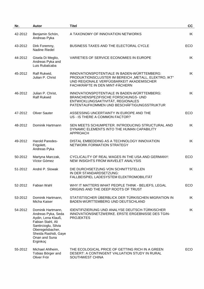
Nr. Autor Titel CC 42-2012 Benjamin Schön,

Andreas Pyka

A TAXONOMY OF INNOVATION NETWORKS IK

43-2012 Dirk Foremny, Nadine Riedel

BUSINESS TAXES AND THE ELECTORAL CYCLE ECO

44-2012 Gisela Di Meglio, Andreas Pyka and Luis Rubalcaba

VARIETIES OF SERVICE ECONOMIES IN EUROPE IK

45-2012 Ralf Rukwid, Julian P. Christ

INNOVATIONSPOTENTIALE IN BADEN-WÜRTTEMBERG: PRODUKTIONSCLUSTER IM BEREICH „METALL, ELEKTRO, IKT“ UND REGIONALE VERFÜGBARKEIT AKADEMISCHER FACHKRÄFTE IN DEN MINT-FÄCHERN

IK

46-2012 Julian P. Christ, Ralf Rukwid

INNOVATIONSPOTENTIALE IN BADEN-WÜRTTEMBERG: BRANCHENSPEZIFISCHE FORSCHUNGS- UND ENTWICKLUNGSAKTIVITÄT, REGIONALES PATENTAUFKOMMEN UND BESCHÄFTIGUNGSSTRUKTUR

IK

47-2012 Oliver Sauter ASSESSING UNCERTAINTY IN EUROPE AND THE US - IS THERE A COMMON FACTOR?

ECO

48-2012 Dominik Hartmann SEN MEETS SCHUMPETER. INTRODUCING STRUCTURAL AND DYNAMIC ELEMENTS INTO THE HUMAN CAPABILITY APPROACH

IK

49-2012 Harold Paredes-Frigolett, Andreas Pyka

DISTAL EMBEDDING AS A TECHNOLOGY INNOVATION NETWORK FORMATION STRATEGY

IK

50-2012 Martyna Marczak, Víctor Gómez

CYCLICALITY OF REAL WAGES IN THE USA AND GERMANY: NEW INSIGHTS FROM WAVELET ANALYSIS

ECO

51-2012 André P. Slowak DIE DURCHSETZUNG VON SCHNITTSTELLEN IN DER STANDARDSETZUNG: FALLBEISPIEL LADESYSTEM ELEKTROMOBILITÄT

IK

52-2012

Fabian Wahl

WHY IT MATTERS WHAT PEOPLE THINK - BELIEFS, LEGAL ORIGINS AND THE DEEP ROOTS OF TRUST

ECO

53-2012

Dominik Hartmann, Micha Kaiser

STATISTISCHER ÜBERBLICK DER TÜRKISCHEN MIGRATION IN BADEN-WÜRTTEMBERG UND DEUTSCHLAND

IK

54-2012

Dominik Hartmann, Andreas Pyka, Seda Aydin, Lena Klauß, Fabian Stahl, Ali Santircioglu, Silvia Oberegelsbacher, Sheida Rashidi, Gaye Onan and Suna Erginkoç

IDENTIFIZIERUNG UND ANALYSE DEUTSCH-TÜRKISCHER INNOVATIONSNETZWERKE. ERSTE ERGEBNISSE DES TGIN-PROJEKTES

IK

55-2012

Michael Ahlheim, Tobias Börger and Oliver Frör

THE ECOLOGICAL PRICE OF GETTING RICH IN A GREEN DESERT: A CONTINGENT VALUATION STUDY IN RURAL SOUTHWEST CHINA

ECO


Matthias Strifler Thomas Beissinger

FAIRNESS CONSIDERATIONS IN LABOR UNION WAGE SETTING – A THEORETICAL ANALYSIS

ECO

57-2012

Peter Spahn

INTEGRATION DURCH WÄHRUNGSUNION? DER FALL DER EURO-ZONE

ECO

58-2012

Sibylle H. Lehmann

TAKING FIRMS TO THE STOCK MARKET: IPOS AND THE IMPORTANCE OF LARGE BANKS IN IMPERIAL GERMANY 1896-1913

ECO

59-2012 Sibylle H. Lehmann,

Philipp Hauber and Alexander Opitz

POLITICAL RIGHTS, TAXATION, AND FIRM VALUATION – EVIDENCE FROM SAXONY AROUND 1900

ECO


SPECTRAN, A SET OF MATLAB PROGRAMS FOR SPECTRAL ANALYSIS

ECO

61-2012 Theresa Lohse, Nadine Riedel

THE IMPACT OF TRANSFER PRICING REGULATIONS ON PROFIT SHIFTING WITHIN EUROPEAN MULTINATIONALS

ECO

Nr. Autor Titel CC 62-2013 Heiko Stüber REAL WAGE CYCLICALITY OF NEWLY HIRED WORKERS ECO

63-2013 David E. Bloom, Alfonso Sousa-Poza

AGEING AND PRODUCTIVITY HCM


MONTHLY US BUSINESS CYCLE INDICATORS: A NEW MULTIVARIATE APPROACH BASED ON A BAND-PASS FILTER

ECO

65-2013 Dominik Hartmann, Andreas Pyka

INNOVATION, ECONOMIC DIVERSIFICATION AND HUMAN DEVELOPMENT

IK

66-2013 Christof Ernst, Katharina Richter and Nadine Riedel

CORPORATE TAXATION AND THE QUALITY OF RESEARCH AND DEVELOPMENT

ECO

67-2013 Michael Ahlheim,

Oliver Frör, Jiang Tong, Luo Jing and Sonna Pelz

NONUSE VALUES OF CLIMATE POLICY - AN EMPIRICAL STUDY IN XINJIANG AND BEIJING

ECO

68-2013 Michael Ahlheim, Friedrich Schneider

CONSIDERING HOUSEHOLD SIZE IN CONTINGENT VALUATION STUDIES

ECO

69-2013 Fabio Bertoni, Tereza Tykvová

WHICH FORM OF VENTURE CAPITAL IS MOST SUPPORTIVE OF INNOVATION? EVIDENCE FROM EUROPEAN BIOTECHNOLOGY COMPANIES

CFRM

70-2013 Tobias Buchmann, Andreas Pyka

THE EVOLUTION OF INNOVATION NETWORKS: THE CASE OF A GERMAN AUTOMOTIVE NETWORK

IK

71-2013 B. Vermeulen, A. Pyka, J. A. La Poutré and A. G. de Kok

CAPABILITY-BASED GOVERNANCE PATTERNS OVER THE PRODUCT LIFE-CYCLE

IK

72-2013

Beatriz Fabiola López Ulloa, Valerie Møller and Alfonso Sousa-Poza

HOW DOES SUBJECTIVE WELL-BEING EVOLVE WITH AGE? A LITERATURE REVIEW

HCM

73-2013

Wencke Gwozdz, Alfonso Sousa-Poza, Lucia A. Reisch, Wolfgang Ahrens, Stefaan De Henauw, Gabriele Eiben, Juan M. Fernández-Alvira, Charalampos Hadjigeorgiou, Eva Kovács, Fabio Lauria, Toomas Veidebaum, Garrath Williams, Karin Bammann

MATERNAL EMPLOYMENT AND CHILDHOOD OBESITY – A EUROPEAN PERSPECTIVE

HCM


Andreas Haas, Annette Hofmann

RISIKEN AUS CLOUD-COMPUTING-SERVICES: FRAGEN DES RISIKOMANAGEMENTS UND ASPEKTE DER VERSICHERBARKEIT

HCM

75-2013

Yin Krogmann, Nadine Riedel and Ulrich Schwalbe

INTER-FIRM R&D NETWORKS IN PHARMACEUTICAL BIOTECHNOLOGY: WHAT DETERMINES FIRM’S CENTRALITY-BASED PARTNERING CAPABILITY?

ECO, IK

76-2013

Peter Spahn

MACROECONOMIC STABILISATION AND BANK LENDING: A SIMPLE WORKHORSE MODEL

ECO

77-2013

Sheida Rashidi, Andreas Pyka

MIGRATION AND INNOVATION – A SURVEY

IK

78-2013

Benjamin Schön, Andreas Pyka

THE SUCCESS FACTORS OF TECHNOLOGY-SOURCING THROUGH MERGERS & ACQUISITIONS – AN INTUITIVE META-ANALYSIS

IK

79-2013

Irene Prostolupow, Andreas Pyka and Barbara Heller-Schuh

TURKISH-GERMAN INNOVATION NETWORKS IN THE EUROPEAN RESEARCH LANDSCAPE

IK

80-2013

Eva Schlenker, Kai D. Schmid

CAPITAL INCOME SHARES AND INCOME INEQUALITY IN THE EUROPEAN UNION

ECO

81-2013 Michael Ahlheim, Tobias Börger and Oliver Frör

THE INFLUENCE OF ETHNICITY AND CULTURE ON THE VALUATION OF ENVIRONMENTAL IMPROVEMENTS – RESULTS FROM A CVM STUDY IN SOUTHWEST CHINA –

ECO

82-2013

Fabian Wahl DOES MEDIEVAL TRADE STILL MATTER? HISTORICAL TRADE CENTERS, AGGLOMERATION AND CONTEMPORARY ECONOMIC DEVELOPMENT

ECO

83-2013 Peter Spahn SUBPRIME AND EURO CRISIS: SHOULD WE BLAME THE ECONOMISTS?

ECO

84-2013 Daniel Guffarth, Michael J. Barber

THE EUROPEAN AEROSPACE R&D COLLABORATION NETWORK

IK

85-2013 Athanasios Saitis KARTELLBEKÄMPFUNG UND INTERNE KARTELLSTRUKTUREN: EIN NETZWERKTHEORETISCHER ANSATZ

IK

Nr. Autor Titel CC 86-2014 Stefan Kirn, Claus D.

Müller-Hengstenberg INTELLIGENTE (SOFTWARE-)AGENTEN: EINE NEUE HERAUSFORDERUNG FÜR DIE GESELLSCHAFT UND UNSER RECHTSSYSTEM?

ICT


MATERNAL EMPLOYMENT AND CHILDHOOD OBESITY IN CHINA: EVIDENCE FROM THE CHINA HEALTH AND NUTRITION SURVEY

HCM

88-2014 Steffen Otterbach, Alfonso Sousa-Poza

JOB INSECURITY, EMPLOYABILITY, AND HEALTH: AN ANALYSIS FOR GERMANY ACROSS GENERATIONS

HCM

89-2014 Carsten Burhop, Sibylle H. Lehmann-Hasemeyer

THE GEOGRAPHY OF STOCK EXCHANGES IN IMPERIAL GERMANY

ECO

90-2014 Martyna Marczak, Tommaso Proietti

OUTLIER DETECTION IN STRUCTURAL TIME SERIES MODELS: THE INDICATOR SATURATION APPROACH

ECO

91-2014 Sophie Urmetzer, Andreas Pyka

VARIETIES OF KNOWLEDGE-BASED BIOECONOMIES IK

92-2014 Bogang Jun, Joongho Lee

THE TRADEOFF BETWEEN FERTILITY AND EDUCATION: EVIDENCE FROM THE KOREAN DEVELOPMENT PATH

IK

93-2014 Bogang Jun, Tai-Yoo Kim

NON-FINANCIAL HURDLES FOR HUMAN CAPITAL ACCUMULATION: LANDOWNERSHIP IN KOREA UNDER JAPANESE RULE

IK

94-2014 Michael Ahlheim, Oliver Frör, Gerhard Langenberger and Sonna Pelz

CHINESE URBANITES AND THE PRESERVATION OF RARE SPECIES IN REMOTE PARTS OF THE COUNTRY – THE EXAMPLE OF EAGLEWOOD

ECO

95-2014 Harold Paredes-Frigolett, Andreas Pyka, Javier Pereira and Luiz Flávio Autran Monteiro Gomes

RANKING THE PERFORMANCE OF NATIONAL INNOVATION SYSTEMS IN THE IBERIAN PENINSULA AND LATIN AMERICA FROM A NEO-SCHUMPETERIAN ECONOMICS PERSPECTIVE

IK

96-2014 Daniel Guffarth, Michael J. Barber

NETWORK EVOLUTION, SUCCESS, AND REGIONAL DEVELOPMENT IN THE EUROPEAN AEROSPACE INDUSTRY

IK

2

IMPRINT

University of HohenheimDean’s Office of the Faculty of Business, Economics and Social SciencesPalace Hohenheim 1 B70593 Stuttgart | GermanyFon +49 (0)711 459 22488Fax +49 (0)711 459 22785E-mail [email protected] Web www.wiso.uni-hohenheim.de

Night lights evidence from South Africa - EconStor

Documents

Transcript of Night lights evidence from South Africa - EconStor