arX

iv:q

uant

-ph/

0309

021v

4 1

3 A

ug 2

005

On the Distribution of the Wave Function for

Systems in Thermal Equilibrium

Sheldon Goldstein∗, Joel L. Lebowitz†,

Roderich Tumulka‡, and Nino Zanghı§

August 12, 2005

Abstract

For a quantum system, a density matrix ρ that is not pure can arise, via

averaging, from a distribution µ of its wave function, a normalized vector belonging

to its Hilbert space H . While ρ itself does not determine a unique µ, additional

facts, such as that the system has come to thermal equilibrium, might. It is thus

not unreasonable to ask, which µ, if any, corresponds to a given thermodynamic

ensemble? To answer this question we construct, for any given density matrix

ρ, a natural measure on the unit sphere in H , denoted GAP (ρ). We do this

using a suitable projection of the Gaussian measure on H with covariance ρ.

We establish some nice properties of GAP (ρ) and show that this measure arises

naturally when considering macroscopic systems. In particular, we argue that it

is the most appropriate choice for systems in thermal equilibrium, described by

the canonical ensemble density matrix ρβ = (1/Z) exp(−βH). GAP (ρ) may also

be relevant to quantum chaos and to the stochastic evolution of open quantum

systems, where distributions on H are often used.

Key words: canonical ensemble in quantum theory; probability measures on

Hilbert space; Gaussian measures; density matrices.

∗Departments of Mathematics and Physics, Hill Center, Rutgers, The State University of New Jersey,

110 Frelinghuysen Road, Piscataway, NJ 08854-8019, USA. E-mail: oldstein@math.rutgers.edu†Departments of Mathematics and Physics, Hill Center, Rutgers, The State University of New Jersey,

110 Frelinghuysen Road, Piscataway, NJ 08854-8019, USA. E-mail: lebowitz@math.rutgers.edu‡Mathematisches Institut, Eberhard-Karls-Universitat, Auf der Morgenstelle 10, 72076 Tubingen,

Germany. E-mail: tumulka@everest.mathematik.uni-tuebingen.de§Dipartimento di Fisica dell’Universita di Genova and INFN sezione di Genova, Via Dodecaneso 33,

16146 Genova, Italy. E-mail: zanghi@ge.infn.it

1

1 Introduction

In classical mechanics, ensembles, such as the microcanonical and canonical ensembles,

are represented by probability distributions on the phase space. In quantum mechan-

ics, ensembles are usually represented by density matrices. It is natural to regard these

density matrices as arising from probability distributions on the (normalized) wave func-

tions associated with the thermodynamical ensembles, so that members of the ensemble

are represented by a random state vector. There are, however, as is well known, many

probability distributions which give rise to the same density matrix, and thus to the

same predictions for experimental outcomes [25, sec. IV.3].1 Moreover, as emphasized

by Landau and Lifshitz [13, sec. I.5], the energy levels for macroscopic systems are so

closely spaced (exponentially small in the number of particles in the system) that “the

concept of stationary states [energy eigenfunctions] becomes in a certain sense unrealis-

tic” because of the difficulty of preparing a system with such a sharp energy and keeping

it isolated. Landau and Lifshitz are therefore wary of, and warn against, regarding the

density matrix for such a system as arising solely from our lack of knowledge about the

wave function of the system. We shall argue, however, that despite these caveats such

distributions can be both useful and physically meaningful. In particular we describe

here a novel probability distribution, to be associated with any thermal ensemble such

as the canonical ensemble.

While probability distributions on wave functions are natural objects of study in

many contexts, from quantum chaos [3, 12, 23] to open quantum systems [4], our main

motivation for considering them is to exploit the analogy between classical and quantum

statistical mechanics [20, 21, 26, 14, 15, 16]. This analogy suggests that some relevant

classical reasonings can be transferred to quantum mechanics by formally replacing the

classical phase space by the unit sphere S (H ) of the quantum system’s Hilbert space

H . In particular, with a natural measure µ(dψ) on S (H ) one can utilize the notion

of typicality, i.e., consider properties of a system common to “almost all” members of

an ensemble. This is a notion frequently used in equilibrium statistical mechanics, as

in, e.g., Boltzmann’s recognition that typical phase points on the energy surface of a

macroscopic system are such that the empirical distribution of velocities is approximately

Maxwellian. Once one has such a measure for quantum systems, one could attempt an

analysis of the second law of thermodynamics in quantum mechanics along the lines of

1This empirical equivalence should not too hastily be regarded as implying physical equivalence.

Consider, for example, the two Schrodinger’s cat states Ψ± = (Ψalive ± Ψdead)/√

2. The measure that

gives equal weight to these two states corresponds to the same density matrix as the one giving equal

weight to Ψalive and Ψdead. However the physical situation corresponding to the former measure, a

mixture of two grotesque superpositions, seems dramatically different from the one corresponding to

the latter, a routine mixture. It is thus not easy to regard these two measures as physically equivalent.

2

Boltzmann’s analysis of the second law in classical mechanics, involving an argument

to the effect that the behavior described in the second law (such as entropy increase)

occurs for typical states of an isolated macroscopic system, i.e. for the overwhelming

majority of points on S (H ) with respect to µ(dψ).

Probability distributions on wave functions of a composite system, with Hilbert

space H , have in fact been used to establish the typical properties of the reduced

density matrix of a subsystem arising from the wave function of the composite. For

example, Page [19] considers the uniform distribution on S (H ) for a finite-dimensional

Hilbert space H , in terms of which he shows that the von Neumann entropy of the

reduced density matrix is typically nearly maximal under appropriate conditions on the

dimensions of the relevant Hilbert spaces.

Given a probability distribution µ on the unit sphere S (H ) of the Hilbert space

H there is always an associated density matrix ρµ [25]: it is the density matrix of the

mixture, or the statistical ensemble of systems, defined by the distribution µ, given by

ρµ =

∫

S (H )

µ(dψ) |ψ〉〈ψ| . (1)

For any projection operator P , tr (ρµP ) is the probability of obtaining in an experiment

a result corresponding to P for a system with a µ-distributed wave function. It is

evident from (1) that ρµ is the second moment, or covariance matrix, of µ, provided µ

has mean 0 (which may, and will, be assumed without loss of generality since ψ and −ψare equivalent physically).

While a probability measure µ on S (H ) determines a unique density matrix ρ on

H via (1), the converse is not true: the association µ 7→ ρµ given by (1) is many-to-

one.2 There is furthermore no unique “physically correct” choice of µ for a given ρ since

for any µ corresponding to ρ one could, in principle, prepare an ensemble of systems

with wave functions distributed according to this µ. However, while ρ itself need not

determine a unique probability measure, additional facts about a system, such as that

it has come to thermal equilibrium, might. It is thus not unreasonable to ask: which

measure on S (H ) corresponds to a given thermodynamic ensemble?

Let us start with the microcanonical ensemble, corresponding to the energy interval

[E,E + δ], where δ is small on the macroscopic scale but large enough for the interval2For example, in a k-dimensional Hilbert space the uniform probability distribution u = uS (H ) over

the unit sphere has density matrix ρu = 1kI with I the identity operator on H ; at the same time, for

every orthonormal basis of H the uniform distribution over the basis (which is a measure concentrated

on just k points) has the same density matrix, ρ = 1kI. An exceptional case is the density matrix

corresponding to a pure state, ρ = |ψ〉〈ψ|, as the measure µ with this density matrix is almost unique:

it must be concentrated on the ray through ψ, and thus the only non-uniqueness corresponds to the

distribution of the phase.

3

to contain many eigenvalues. To this there is associated the spectral subspace HE,δ,

the span of the eigenstates |n〉 of the Hamiltonian H corresponding to eigenvalues Enbetween E and E+ δ. Since HE,δ is finite dimensional, one can form the microcanonical

density matrix

ρE,δ = (dim HE,δ)−1PHE,δ

(2)

with PHE,δ= 1[E,E+δ](H) the projection to HE,δ. This density matrix is diagonal in the

energy representation and gives equal weight to all energy eigenstates in the interval

[E,E + δ].

But what is the corresponding microcanonical measure? The most plausible answer,

given long ago by Schrodinger [20, 21] and Bloch [26], is the (normalized) uniform

measure uE,δ = uS (HE,δ) on the unit sphere in this subspace. ρE,δ is associated with uE,δvia (1).

Note that a wave function Ψ chosen at random from this distribution is almost cer-

tainly a nontrivial superposition of the eigenstates |n〉 with random coefficients 〈n|Ψ〉that are identically distributed, but not independent. The measure uE,δ is clearly sta-

tionary, i.e., invariant under the unitary time evolution generated by H , and it is as

spread out as it could be over the set S (HE,δ) of allowed wave functions. This measure

provides us with a notion of a “typical wave function” from HE,δ which is very different

from the one arising from the measure µE,δ that, when H is nondegenerate, gives equal

probability (dim HE,δ)−1 to every eigenstate |n〉 with eigenvalue En ∈ [E,E + δ]. The

measure µE,δ, which is concentrated on these eigenstates, is, however, less robust to

small perturbations in H than is the smoother measure uE,δ.

Our proposal for the canonical ensemble is in the spirit of the uniform microcanonical

measure uE,δ and reduces to it in the appropriate cases. It is based on a mathematically

natural family of probability measures µ on S (H ). For every density matrix ρ on

H , there is a unique member µ of this family, satisfying (1) for ρµ = ρ, namely the

Gaussian adjusted projected measure GAP (ρ), constructed roughly as follows: Eq. (1)

(i.e., the fact that ρµ is the covariance of µ) suggests that we start by considering the

Gaussian measure G(ρ) with covariance ρ (and mean 0), which could, in finitely many

dimensions, be expressed by G(ρ)(dψ) ∝ exp(−〈ψ|ρ−1|ψ〉) dψ (where dψ is the obvious

Lebesgue measure on H ).3 This is not adequate, however, since the measure that we

seek must live on the sphere S (H ) whereas G(ρ) is spread out over all of H . We

thus adjust and then project G(ρ) to S (H ), in the manner described in Section 2,

in order to obtain the measure GAP (ρ), having the prescribed covariance ρ as well as

3Berry [3] has conjectured, and for some cases proven, that such measures describe interesting

universal properties of chaotic energy eigenfunctions in the semiclassical regime, see also [12, 23]. It

is perhaps worth considering the possibility that the GAP measures described here provide somewhat

better candidates for this purpose.

4

other desirable properties.

It is our contention that a quantum system in thermal equilibrium at inverse tem-

perature β should be described by a random state vector whose distribution is given by

the measure GAP (ρβ) associated with the density matrix for the canonical ensemble,

ρβ = ρH ,H,β =1

Zexp(−βH) with Z := tr exp(−βH). (3)

In order to convey the significance of GAP (ρ) as well as the plausibility of our

proposal that GAP (ρβ) describes thermal equilibrium, we recall that a system described

by a canonical ensemble is usually regarded as a subsystem of a larger system. It is

therefore important to consider the notion of the distribution of the wave function of a

subsystem. Consider a composite system in a pure state ψ ∈ H1 ⊗ H2, and ask what

might be meant by the wave function of the subsystem with Hilbert space H1. For

this we propose the following. Let |q2〉 be a (generalized) orthonormal basis of H2

(playing the role, say, of the eigenbasis of the position representation). For each choice

of |q2〉, the (partial) scalar product 〈q2|ψ〉, taken in H2, is a vector belonging to H1.

Regarding |q2〉 as random, we are led to consider the random vector Ψ1 ∈ H1 given by

Ψ1 = N 〈Q2|ψ〉 (4)

where N = N (ψ,Q2) =∥

∥〈Q2|ψ〉∥

∥

−1is the normalizing factor and |Q2〉 is a random

element of the basis |q2〉, chosen with the quantum distribution

P(Q2 = q2) =∥

∥〈q2|ψ〉∥

∥

2. (5)

We refer to Ψ1 as the conditional wave function [6] of system 1. Note that Ψ1 becomes

doubly random when we start with a random wave function in H1 ⊗ H2 instead of a

fixed one.

The distribution of Ψ1 corresponding to (4) and (5) is given by the probability

measure on S (H1),

µ1(dψ1) = P(Ψ1 ∈ dψ1) =∑

q2

∥

∥〈q2|ψ〉∥

∥

2δ(

ψ1 −N (ψ, q2) 〈q2|ψ〉)

dψ1 , (6)

where δ(ψ − φ) dψ denotes the “delta” measure concentrated at φ. While the density

matrix ρµ1associated with µ1 always equals the reduced density matrix ρred

1 of system

1, given by

ρred1 = tr2|ψ〉〈ψ| =

∑

q2

〈q2|ψ〉〈ψ|q2〉 , (7)

the measure µ1 itself usually depends on the choice of the basis |q2〉. It turns out,

nevertheless, as we point out in Section 5.1, that µ1(dψ1) is a universal function of ρred1

5

in the special case that system 2 is large and ψ is typical (with respect to the uni-

form distribution on all wave functions with the same reduced density matrix), namely

GAP (ρred1 ). Thus GAP (ρ) has a distinguished, universal status among all probability

measures on S (H ) with density matrix ρ.

To further support our claim that GAP (ρβ) is the right measure for ρβ , we shall

regard, as is usually done, the system described by ρβ as coupled to a (very large)

heat bath. The interaction between the heat bath and the system is assumed to be

(in some suitable sense) negligible. We will argue that if the wave function ψ of the

combined “system plus bath” has microcanonical distribution uE,δ, then the distribution

of the conditional wave function of the (small) system is approximately GAP (ρβ); see

Section 4.

Indeed, a stronger statement is true. As we argue in Section 5.2, even for a typical

fixed microcanonical wave function ψ of the composite, i.e., one typical for uE,δ, the

conditional wave function of the system, defined in (4), is then approximately GAP (ρβ)-

distributed, for a typical basis |q2〉. This is related to the fact that for a typical

microcanonical wave function ψ of the composite the reduced density matrix for the

system is approximately ρβ [7, 21]. Note that the analogous statement in classical

mechanics would be wrong: for a fixed phase point ξ of the composite, be it typical or

atypical, the phase point of the system could never be random, but rather would merely

be the part of ξ belonging to the system.

The remainder of this paper is organized as follows. In Section 2 we define the

measure GAP (ρ) and obtain several ways of writing it. In Section 3 we describe some

natural mathematical properties of these measures, and suggest that these properties

uniquely characterize the measures. In Section 4 we argue that GAP (ρβ) represents the

canonical ensemble. In Section 5 we outline the proof that GAP (ρ) is the distribution

of the conditional wave function for most wave functions in H1 ⊗ H2 with reduced

density matrix ρ if system 2 is large, and show that GAP (ρβ) is the typical distribution

of the conditional wave function arising from a fixed microcanonical wave function of

a system in contact with a heat bath. In Section 6 we discuss other measures that

have been or might be considered as the thermal equilibrium distribution of the wave

function. Finally, in Section 7 we compute explicitly the distribution of the coefficients

of a GAP (ρβ)-distributed state vector in the simplest possible example, the two-level

system.

2 Definition of GAP (ρ)

In this section, we define, for any given density matrix ρ on a (separable) Hilbert space

H , the Gaussian adjusted projected measure GAP (ρ) on S (H ). This definition makes

6

use of two auxiliary measures, G(ρ) and GA(ρ), defined as follows.

G(ρ) is the Gaussian measure on H with covariance matrix ρ (and mean 0). More

explicitly, let |n〉 be an orthonormal basis of eigenvectors of ρ and pn the corresponding

eigenvalues,

ρ =∑

n

pn |n〉〈n|. (8)

Such a basis exists because ρ has finite trace. Let Zn be a sequence of independent

complex-valued random variables having a (rotationally symmetric) Gaussian distribu-

tion in C with mean 0 and variance

E|Zn|2 = pn (9)

(where E means expectation), i.e., ReZn and ImZn are independent real Gaussian

variables with mean zero and variance pn/2. We define G(ρ) to be the distribution of

the random vector

ΨG :=∑

n

Zn|n〉 . (10)

Note that ΨG is not normalized, i.e., it does not lie in S (H ). In order that ΨG lie in

H at all, we need that the sequence Zn be square-summable,∑

n |Zn|2 <∞. That this

is almost surely the case follows from the fact that E∑

n |Zn|2 is finite. In fact,

E∑

n

|Zn|2 =∑

n

E|Zn|2 =∑

n

pn = tr ρ = 1. (11)

More generally, we observe that for any measure µ on H with (mean 0 and) covariance

given by the trace class operator C,

∫

H

µ(dψ) |ψ〉〈ψ| = C ,

we have that, for a random vector Ψ with distribution µ, E‖Ψ‖2 = trC.

It also follows that ΨG almost surely lies in the positive spectral subspace of ρ, the

closed subspace spanned by those |n〉 with pn 6= 0, or, equivalently, the orthogonal

complement of the kernel of ρ; we shall call this subspace support(ρ). Note further that,

since G(ρ) is the Gaussian measure with covariance ρ, it does not depend (in the case

of degenerate ρ) on the choice of the basis |n〉 among the eigenbases of ρ, but only on

ρ.

Since we want a measure on S (H ) while G(ρ) is not concentrated on S (H ) but

rather is spread out, it would be natural to project G(ρ) to S (H ). However, since

projecting to S (H ) changes the covariance of a measure, as we will point out in detail

in Section 3.1, we introduce an adjustment factor that exactly compensates for the

7

change of covariance due to projection. We thus define the adjusted Gaussian measure

GA(ρ) on H by

GA(ρ)(dψ) = ‖ψ‖2 G(ρ)(dψ). (12)

Since E‖ΨG‖2 = 1 by (11), GA(ρ) is a probability measure.

Let ΨGA be a GA(ρ)-distributed random vector. We define GAP (ρ) to be the dis-

tribution of

ΨGAP :=ΨGA

‖ΨGA‖ = P (ΨGA) (13)

with P the projection to the unit sphere (i.e., the normalization of a vector),

P : H \ 0 → S (H ) , P (ψ) = ‖ψ‖−1ψ. (14)

Putting (13) differently, for a subset B ⊆ S (H ),

GAP (ρ)(B) = GA(ρ)(R+B) =

∫

R+B

G(ρ)(dψ) ‖ψ‖2 (15)

where R+B denotes the cone through B. More succinctly,

GAP (ρ) = P∗

(

GA(ρ))

= GA(ρ) P−1 . (16)

where P∗ denotes the action of P on measures.

More generally, one can define for any measure µ on H the “adjust-and-project”

procedure: let A(µ) be the adjusted measure A(µ)(dψ) = ‖ψ‖2 µ(dψ); then the adjusted-

and-projected measure is P∗

(

A(µ))

= A(µ) P−1, thus defining a mapping P∗ A from

the measures on H with∫

µ(dψ) ‖ψ‖2 = 1 to the probability measures on S (H ). We

then have that GAP (ρ) = P∗

(

A(G(ρ)))

.

We remark that ΨGAP , too, lies in support(ρ) almost surely, and that P (ΨG) does

not have distribution GAP (ρ)—nor covariance ρ (see Sect. 3.1).

We can be more explicit in the case that ρ has finite rank k = dim support(ρ), e.g. for

finite-dimensional H : then there exists a Lebesgue volume measure λ on support(ρ) =

Ck, and we can specify the densities of G(ρ) and GA(ρ),

dG(ρ)

dλ(ψ) =

1

πk det ρ+exp(−〈ψ|ρ−1

+ |ψ〉), (17a)

dGA(ρ)

dλ(ψ) =

‖ψ‖2

πk det ρ+

exp(−〈ψ|ρ−1+ |ψ〉), (17b)

with ρ+ the restriction of ρ to support(ρ). Similarly, we can express GAP (ρ) relative to

8

the (2k − 1)–dimensional surface measure u on S (support(ρ)),

dGAP (ρ)

du(ψ) =

1

πk det ρ+

∞∫

0

dr r2k−1 r2 exp(−r2〈ψ|ρ−1+ |ψ〉) = (18a)

=k!

2πk det ρ+〈ψ|ρ−1

+ |ψ〉−k−1 . (18b)

We note that

GAP (ρE,δ) = uE,δ , (19)

where ρEδ is the microcanonical density matrix given in (2) and uEδ is the microcanonical

measure.

3 Properties of GAP (ρ)

In this section we prove the following properties of GAP (ρ):

Property 1 The density matrix associated with GAP (ρ) in the sense of (1) is ρ, i.e.,

ρGAP (ρ) = ρ.

Property 2 The association ρ 7→ GAP (ρ) is covariant: For any unitary operator U on

H ,

U∗GAP (ρ) = GAP (UρU∗) (20)

where U∗ = U−1 is the adjoint of U and U∗ is the action of U on measures, U∗µ = µU−1.

In particular, GAP (ρ) is stationary under any unitary evolution that preserves ρ.

Property 3 If Ψ ∈ H1 ⊗ H2 has distribution GAP (ρ1 ⊗ ρ2) then, for any basis |q2〉of H2, the conditional wave function Ψ1 has distribution GAP (ρ1). (“GAP of a product

density matrix has GAP marginal.”)

We will refer to the property expressed in Property 3 by saying that the family of

GAP measures is hereditary. We note that when Ψ ∈ H1⊗H2 has distribution GAP (ρ)

and ρ is not a tensor product, the distribution of Ψ1 need not be GAP (ρred1 ) (as we will

show after the proof of Property 3).

Before establishing these properties let us formulate what they say about our can-

didate GAP (ρβ) for the canonical distribution. As a consequence of Property 1, the

density matrix arising from µ = GAP (ρβ) in the sense of (1) is the density matrix ρβ .

As a consequence of Property 2, GAP (ρβ) is stationary, i.e., invariant under the unitary

time evolution generated by H . As a consequence of Property 3, if Ψ ∈ H = H1 ⊗H2

has distribution GAP (ρH ,H,β) and systems 1 and 2 are decoupled, H = H1⊗I2+I1⊗H2,

9

where Ii is the identity on Hi, then the conditional wave function Ψ1 of system 1 has

a distribution (in H1) of the same kind with the same inverse temperature β, namely

GAP (ρH1,H1,β). This fits well with our claim that GAP (ρβ) is the thermal equilibrium

distribution since one would expect that if a system is in thermal equilibrium at inverse

temperature β then so are its subsystems.

We conjecture that the family of GAP measures is the only family of measures

satisfying Properties 1–3. This conjecture is formulated in detail, and established for

suitably continuous families of measures, in Section 6.2.

The following lemma, proven in Section 3.3, is convenient for showing that a random

wave function is GAP-distributed:

Lemma 1 Let Ω be a measurable space, µ a probability measure on Ω, and Ψ : Ω → H

a Hilbert-space-valued function. If Ψ(ω) is G(ρ)-distributed with respect to µ(dω), then

Ψ(ω)/‖Ψ(ω)‖ is GAP (ρ)-distributed with respect to ‖Ψ(ω)‖2µ(dω).

3.1 The Density Matrix

In this subsection we establish Property 1. We then add a remark on the covariance

matrix.

Proof of Property 1. From (1) we find that

ρGAP (ρ) =

∫

S (H )

GAP (ρ)(dψ) |ψ〉〈ψ| = E

(

|ΨGAP 〉〈ΨGAP |)

=

(13)= E

(

‖ΨGA‖−2 |ΨGA〉〈ΨGA|)

=

∫

H

GA(ρ)(dψ) ‖ψ‖−2 |ψ〉〈ψ| =

(12)=

∫

H

G(ρ)(dψ) |ψ〉〈ψ| = ρ

because∫

HG(ρ)(dψ) |ψ〉〈ψ| is the covariance matrix of G(ρ), which is ρ. (A number

above an equal sign refers to the equation used to obtain the equality.)

Remark on the covariance matrix. The equation ρGAP (ρ) = ρ can be understood as

expressing that GAP (ρ) and G(ρ) have the same covariance. For a probability measure

µ on H with mean 0 that need not be concentrated on S (H ), the covariance matrix

Cµ is given by

Cµ =

∫

H

µ(dφ) |φ〉〈φ|. (21)

10

Suppose we want to obtain from µ a probability measure on S (H ) having the same

covariance. The projection P∗µ of µ to S (H ), defined by P∗µ(B) = µ(R+B) for

B ⊆ S (H ), is not what we want, as it has covariance

CP∗µ =

∫

S (H )

P∗µ(dψ) |ψ〉〈ψ| =

∫

H

µ(dφ) ‖φ‖−2 |φ〉〈φ| 6= Cµ.

However, P∗

(

A(µ))

does the job: it has the same covariance. As a consequence, a nat-

urally distinguished measure on S (H ) with given covariance is the Gaussian adjusted

projected measure, the GAP measure, with the given covariance.

3.2 GAP (ρ) is Covariant

We establish Property 2 and then discuss in more general terms under which conditions

a measure on S (H ) is stationary.

Proof of Property 2. Under a unitary transformation U , a Gaussian measure with covari-

ance matrix C transforms into one with covariance matrix UCU∗. Since ‖Uψ‖2 = ‖ψ‖2,

GA(C) transforms into GA(UCU∗); that is, UΨGAC and ΨGA

UCU∗ are equal in distribution,

and since ‖UΨGAC ‖ = ‖ΨGA

C ‖, we have that UΨGAPC and ΨGAP

UCU∗ are equal in distribution.

In other words, GAP (C) transforms into GAP (UCU∗), which is what we claimed in

(20).

3.2.1 Stationarity

In this subsection we discuss a criterion for stationarity under the evolution generated

by H =∑

nEn |n〉〈n|. Consider the following property of a sequence of complex random

variables Zn:

The phases Zn/|Zn|, when they exist, are independent of the moduli |Zn|and of each other, and are uniformly distributed on S1 = eiθ : θ ∈ R.

(22)

(The phase Zn/|Zn| exists when Zn 6= 0.) Condition (22) implies that the distribution

of the random vector Ψ =∑

n Zn|n〉 is stationary, since Zn(t) = exp(−iEnt/~)Zn(0).

Note also that (22) implies that the distribution has mean 0.

We show that the Zn = 〈n|ΨGAP 〉 have property (22). To begin with, the Zn =

〈n|ΨG〉 obviously have this property since they are independent Gaussian variables.

Since the density of GA(ρ) relative to G(ρ) is a function of the moduli alone, also the

Zn = 〈n|ΨGA〉 satisfy (22). Finally, since the |〈n|ΨGAP 〉| are functions of the |〈n|ΨGA〉|while the phases of the 〈n|ΨGAP 〉 equal the phases of the 〈n|ΨGA〉, also the Zn =

〈n|ΨGAP 〉 satisfy (22).

11

We would like to add that (22) is not merely a sufficient, but also almost a necessary

condition (and morally a necessary condition) for stationarity. Since for any Ψ, the

moduli |Zn| = |〈n|Ψ〉| are constants of the motion, the evolution of Ψ takes place in the

(possibly infinite-dimensional) torus

∑

n

|Zn|eiθn |n〉 : 0 ≤ θn < 2π

∼=∏

n:Zn 6=0

S1, (23)

contained in S (H ). Independent uniform phases correspond to the uniform measure λ

on∏

n S1. λ is the only stationary measure if the motion on

∏

n S1 is uniquely ergodic,

and this is the case whenever the spectrum En of H is linearly independent over

the rationals Q, i.e., when every finite linear combination∑

n rnEn of eigenvalues with

rational coefficients rn, not all of which vanish, is nonzero, see [2, 24].

This is true of generic Hamiltonians, so that λ is generically the unique stationary

distribution on the torus. But even when the spectrum of H is linearly dependent,

e.g. when there are degenerate eigenvalues, and thus further stationary measures on

the torus exist, these further measures should not be relevant to thermal equilibrium

measures, because of their instability against perturbations of H [11, 1].

The stationary measure λ on∏

n S1 corresponds, for given moduli |Zn| or, equiva-

lently, by setting |Zn| = p(En)1/2 for a given probability measure p on the spectrum of

H , to a stationary measure λp on S (H ) that is concentrated on the embedded torus

(23). The measures λp are (for generic H) the extremal stationary measures, i.e., the

extremal elements of the convex set of stationary measures, of which all other stationary

measures are mixtures.

3.3 GAP Measures and Gaussian Measures

Lemma 1 is more or less immediate from the definition of GAP (ρ). A more detailed

proof looks like this:

Proof of Lemma 1. By assumption the distribution µ Ψ−1 of Ψ with respect to µ is

G(ρ). Thus for the distribution of Ψ with respect to µ′(dω) = ‖Ψ(ω)‖2µ(dω), we have

µ′ Ψ−1(dψ) = ‖ψ‖2 µ Ψ−1(dψ) = ‖ψ‖2G(ρ)(dψ) = GA(ρ)(dψ). Thus, P (Ψ(ω)) has

distribution P∗GA(ρ) = GAP (ρ).

3.4 Generalized Bases

We have already remarked in the introduction that the orthonormal basis |q2〉 of H2,

used in the definition of the conditional wave function, could be a generalized basis, such

12

as a “continuous” basis, for which it is appropriate to write

I2 =

∫

dq2 |q2〉〈q2|

instead of the “discrete” notation

I2 =∑

q2

|q2〉〈q2|

we used in (4)–(7).

We wish to elucidate this further. A generalized orthonormal basis |q2〉 : q2 ∈ Q2indexed by the set Q2 is mathematically defined by a unitary isomorphism H2 →L2(Q2, dq2), where dq2 denotes a measure on Q2. We can think of Q2 as the configuration

space of system 2; as a typical example, system 2 may consist of N2 particles in a box

Λ ⊂ R3, so that its configuration space is Q2 = ΛN2 with dq2 the Lebesgue measure

(which can be regarded as obtained by combining N2 copies of the volume measure on

R3).4 The formal ket |q2〉 then means the delta function centered at q2; it is to be treated

as (though strictly speaking it is not) an element of H2.

The definition of the conditional wave function Ψ1 then reads as follows: The vector

ψ ∈ H1 ⊗H2 can be regarded, using the isomorphism H2 → L2(Q2, dq2), as a function

ψ : Q2 → H1. Eq. (4) is to be understood as meaning

Ψ1 = N ψ(Q2) (24)

where

N = N (ψ,Q2) =∥

∥ψ(Q2)∥

∥

−1

is the normalizing factor and Q2 is a random point in Q2, chosen with the quantum

distribution

P(Q2 ∈ dq2) =∥

∥ψ(q2)∥

∥

2dq2 , (25)

which is how (5) is to be understood in this setting. As ψ is defined only up to changes

on a null set in Q2, Ψ1 may not be defined for a particular Q2. Its distribution in

H1, however, is defined unambiguously by (24). In the most familiar setting with

H1 = L2(Q1, dq1), we have that (ψ(Q2))(q1) = ψ(q1, Q2).

In the following, we will allow generalized bases and use continuous instead of discrete

notation, and set 〈Q2|ψ〉 = ψ(Q2).

4In fact, in the original definition of the conditional wave function in [6], q2 was supposed to be the

configuration, corresponding to the positions of the particles belonging to system 2. For our purposes

here, however, the physical meaning of the q2 is irrelevant, so that any generalized orthonormal basis

of H2 can be used.

13

3.5 Distribution of the Wave Function of a Subsystem

Proof of Property 3. The proof is divided into four steps.

Step 1. We can assume that Ψ = P (ΨGA) where ΨGA is a GA(ρ)-distributed random

vector in H = H1 ⊗ H2. We then have that Ψ1 = P1

(

〈Q2|Ψ〉)

= P1

(

〈Q2|ΨGA〉)

where

P1 is the normalization in H1, and where the distribution of Q2, given ΨGA, is

P(Q2 ∈ dq2|ΨGA) =‖〈q2|ΨGA〉‖2

‖ΨGA‖2dq2 .

ΨGA and Q2 have a joint distribution given by the following measure ν on H ×Q2:

ν(dψ × dq2) = ‖〈q2|ψ〉‖2G(ρ)(dψ) dq2 . (26)

Thus, what needs to be shown is that with respect to ν, P1(〈q2|ψ〉) is GAP (ρ1)-

distributed.

Step 2. If Ψ ∈ H1 ⊗ H2 is G(ρ1 ⊗ ρ2)-distributed and q2 ∈ Q2 is fixed, then the

random vector f(q2) 〈q2|Ψ〉 ∈ H1 with f(q2) = 〈q2|ρ2|q2〉−1/2 is G(ρ1)-distributed. This

follows, more or less, from the fact that a subset of a set of jointly Gaussian random

variables is also jointly Gaussian, together with the observation that the covariance of

〈q2|Ψ〉 is

∫

H

G(ρ1 ⊗ ρ1)(dψ) 〈q2|ψ〉〈ψ|q2〉 = 〈q2|ρ1 ⊗ ρ2|q2〉 = ρ1 〈q2|ρ2|q2〉 .

More explicitly, pick an orthonormal basis |ni〉 of Hi consisting of eigenvectors of

ρi with eigenvalues p(i)ni , and note that the vectors |n1, n2〉 := |n1〉 ⊗ |n2〉 form an or-

thonormal basis of H = H1 ⊗H2 consisting of eigenvectors of ρ1 ⊗ ρ2 with eigenvalues

pn1,n2= p

(1)n1 p

(2)n2 . Since the random variables Zn1,n2

:= 〈n1, n2|Ψ〉 are independent Gaus-

sian random variables with mean zero and variances E|Zn1, n2|2 = pn1,n2

, so are their

linear combinations

Z(1)n1:= 〈n1|f(q2) Ψ(q2)〉 = f(q2)

∑

n2

〈q2|n2〉Zn1,n2

with variances (because variances add when adding independent Gaussian random vari-

ables)

E|Z(1)n1|2 = f 2(q2)

∑

n2

∣

∣〈q2|n2〉∣

∣

2E|Zn1,n2

|2 = p(1)n1

∑

n2|〈q2|n2〉|2 p(2)

n2

〈q2|ρ2|q2〉= p(1)

n1.

Thus f(q2) 〈q2|Ψ〉 is G(ρ1)-distributed, which completes step 2.

14

Step 3. If Ψ ∈ H1 ⊗ H2 is G(ρ1 ⊗ ρ2)-distributed and Q2 ∈ Q2 is random with any

distribution, then the random vector f(Q2) 〈Q2|Ψ〉 is G(ρ1)-distributed. This is a trivial

consequence of step 2.

Step 4. Apply Lemma 1 as follows. Let Ω = H ×Q2, Ψ(ω) = Ψ(ψ, q2) = f(q2) 〈q2|ψ〉,and µ(dψ×dq2) = G(ρ)(dψ) 〈q2|ρ2|q2〉 dq2 (which means that q2 and ψ are independent).

By step 3, the hypothesis of Lemma 1 (for ρ = ρ1) is satisfied, and thus P1(Ψ) =

P1(〈q2|ψ〉) is GAP (ρ1)-distributed with respect to

‖Ψ(ω)‖2µ(dω) = f 2(q2)‖〈q2|ψ〉‖2G(ρ)(dψ) 〈q2|ρ2|q2〉 dq2 = ν(dω) ,

where we have used that f 2(q2) = 〈q2|ρ2|q2〉−1. But this is, according to step 1, what

we needed to show.

To verify the statement after Property 3, consider the density matrix ρ = |Φ〉〈Φ| for

a pure state Φ of the form Φ =∑

n

√pn ψn ⊗ φn, where ψn and φn are respectively

orthonormal bases for H1 and H2 and the pn are nonnegative with∑

n pn = 1. Then

a GAP (ρ)-distributed random vector Ψ coincides with Φ up to a random phase, and

so ρred1 =

∑

n pn |ψn〉〈ψn|. Choosing for |q2〉 the basis φn, the distribution of Ψ1 is

not GAP (ρred1 ) but rather is concentrated on the eigenvectors of ρred

1 . When the pn are

pairwise-distinct this measure is the measure EIG(ρred1 ) we define in Section 6.1.1.

4 Microcanonical Distribution for a Large System

Implies the Distribution GAP (ρβ) for a Subsystem

In this section we use Property 3, i.e., the fact that GAP measures are hereditary, to show

that GAP (ρβ) is the distribution of the conditional wave function of a system coupled

to a heat bath when the wave function of the composite is distributed microcanonically,

i.e., according to uE,δ.

Consider a system with Hilbert space H1 coupled to a heat bath with Hilbert space

H2. Suppose the composite system has a random wave function Ψ ∈ H = H1 ⊗ H2

whose distribution is microcanonical, uE,δ. Assume further that the coupling is negligibly

small, so that we can write for the Hamiltonian

H = H1 ⊗ I2 + I1 ⊗H2 , (27)

and that the heat bath is large (so that the energy levels of H2 are very close).

It is a well known fact that for macroscopic systems different equilibrium ensembles,

for example the microcanonical and the canonical, give approximately the same answer

for appropriate quantities. By this equivalence of ensembles [17], we should have that

15

ρE,δ ≈ ρβ for suitable β = β(E). Then, since GAP (ρ) depends continuously on ρ, we

have that uE,δ = GAP (ρE,δ) ≈ GAP (ρβ). Thus we should have that the distribution

of the conditional wave function Ψ1 of the system is approximately the same as would

be obtained when Ψ is GAP (ρβ)-distributed. But since, by (27), the canonical density

matrix is then of the form

ρβ = ρH ,H,β = ρH1,H1,β ⊗ ρH2,H2,β , (28)

we have by Property 3 that Ψ1 is approximately GAP (ρH1,H1,β)-distributed, which is

what we wanted to show.

5 Typicality of GAP Measures

The previous section concerns the distribution of the conditional wave function Ψ1 aris-

ing from the microcanonical distribution of the wave function of the composite. It

concerns, in other words, a random wave function of the composite. The result there is

the analogue, on the level of measures on Hilbert space, of the well known result that if

a microcanonical density matrix (2) is assumed for the composite, the reduced density

matrix ρred1 of the system, defined as the partial trace tr2 ρE,δ, is canonical if the heat

bath is large [13].

As indicated in the introduction, a stronger statement about the canonical density

matrix is in fact true, namely that for a fixed (nonrandom) wave function ψ of the

composite which is typical with respect to uE,δ, ρred1 ≈ ρH1,H1,β when the heat bath is

large (see [7, 21]; for a rigorous study of special cases of a similar question, see [22]).5

This stronger statement will be used in Section 5.2 to show that a similar statement

holds for the distribution of Ψ1 as well, namely that it is approximately GAP (ρH1,H1,β)-

distributed for a typical fixed ψ ∈ HE,δ and basis |q2〉 of H2. But we must first

consider the distribution of Ψ1 for a typical ψ ∈ H .

5.1 Typicality of GAP Measures for a Subsystem of a Large

System

In this section we argue that for a typical wave function of a big system the conditional

wave function of a small subsystem is approximately GAP-distributed, first giving a

precise formulation of this result and then sketching its proof. We give the detailed

proof in [8].

5It is a consequence of the results in [19] that when dim H2 → ∞, the reduced density matrix be-

comes proportional to the identity on H1 for typical wave functions relative to the uniform distribution

on S (H ) (corresponding to uE,δ for E = 0 and H = 0).

16

5.1.1 Statement of the Result

Let H = H1 ⊗ H2, where H1 and H2 have respective dimensions k and m, with

k < m <∞. For any given density matrix ρ1 on H1, consider the set

R(ρ1) =

ψ ∈ S (H ) : ρred1 (ψ) = ρ1

, (29)

where ρred1 (ψ) = tr2|ψ〉〈ψ| is the reduced density matrix for the wave function ψ. There

is a natural notion of (normalized) uniform measure uρ1 on R(ρ1); we give its precise

definition in Section 5.1.3.

We claim that for fixed k and large m, the distribution µψ1 of the conditional wave

function Ψ1 of system 1, defined by (4) and (5) for a basis |q2〉 of H2, is close to

GAP (ρ1) for the overwhelming majority, relative to uρ1 , of vectors ψ ∈ H with reduced

density matrix ρ1. More precisely:

For every ε > 0 and every bounded continuous function f : S (H1) → R,

uρ1

ψ ∈ R(ρ1) :∣

∣µψ1 (f) −GAP (ρ1)(f)∣

∣ < ε

→ 1 as m→ ∞ , (30)

regardless of how the basis |q2〉 is chosen.

Here we use the notation

µ(f) :=

∫

S (H )

µ(dψ) f(ψ) . (31)

5.1.2 Measure on H Versus Density Matrix

It is important to resist the temptation to translate uρ1 into a density matrix in H .

As mentioned in the introduction, to every probability measure µ on S (H ) there

corresponds a density matrix ρµ in H , given by (1), which contains all the empirically

accessible information about an ensemble with distribution µ. It may therefore seem

a natural step to consider, instead of the measure µ = uρ1, directly its density matrix

ρµ = 1mρ1⊗I2, where I2 is the identity on H2. But since our result concerns properties of

most wave functions relative to µ, it cannot be formulated in terms of the density matrix

ρµ. In particular, the corresponding statement relative to another measure µ′ 6= µ on

S (H ) with the same density matrix ρµ′ = ρµ could be false. Noting that ρµ has a basis

of eigenstates that are product vectors, we could, for example, take µ′ to be a measure

concentrated on these eigenstates. For any such state ψ, µψ1 is a delta-measure.

17

5.1.3 Outline of Proof

The result follows, by (5), Lemma 1, and the continuity of P∗A, from the corresponding

statement about the Gaussian measure G(ρ1) on H1 with covariance ρ1:

For every ε > 0 and every bounded continuous f : H1 → R,

uρ1

ψ ∈ R(ρ1) :∣

∣µψ1 (f) −G(ρ1)(f)∣

∣ < ε

→ 1 as m→ ∞ , (32)

where µψ1 is the distribution of√m 〈Q2|ψ〉 ∈ H1 (not normalized) with respect to the

uniform distribution of Q2 ∈ 1, . . . , m.

We sketch the proof of (32) and give the definition of uρ1. According to the Schmidt

decomposition, every ψ ∈ H can be written in the form

ψ =∑

i

ci χi ⊗ φi , (33)

where χi is an orthonormal basis of H1, φi an orthonormal system in H2, and the

ci are coefficients which can be assumed real and nonnegative. From (33) one reads off

the reduced density matrix of system 1,

ρred1 =

∑

i

c2i |χi〉〈χi| . (34)

As the reduced density matrix is given, ρred1 = ρ1, the orthonormal basis χi and the

coefficients ci are determined (when ρ1 is nondegenerate) as the eigenvectors and the

square-roots of the eigenvalues of ρ1, and, R(ρ1) is in a natural one-to-one correspon-

dence with the set ONS(H2, k) of all orthonormal systems φi in H2 of cardinality

k. (If some of the eigenvalues of ρ1 vanish, the one-to-one correspondence is with

ONS(H2, k′) where k′ = dim support(ρ1).) The Haar measure on the unitary group of

H2 defines the uniform distribution on the set of orthonormal bases of H2, of which

the uniform distribution on ONS(H2, k) is a marginal, and thus defines the uniform

distribution uρ1 on R(ρ1). (When ρ1 is degenerate, uρ1 does not depend upon how the

eigenvectors χi of ρ1 are chosen.)

The key idea for establishing (32) from the Schmidt decomposition (33) is this: µψ1is the average of m delta measures with equal weights, µψ1 = m−1

∑

q2δψ1(q2), located at

the points

ψ1(q2) =k

∑

i=1

ci√m 〈q2|φi〉χi . (35)

Now regard ψ as random with distribution uρ1; then the ψ1(q2) are m random vectors,

and µψ1 is their empirical distribution. If the mk coefficients 〈q2|φi〉 were independent

18

Gaussian (complex) random variables with (mean zero and) variance m−1, then the

ψ1(q2) would be m independent drawings of a G(ρ1)-distributed random vector; by the

weak law of large numbers, their empirical distribution would usually be close to G(ρ1);

in fact, the probability that∣

∣µψ1 (f) −G(ρ1)(f)∣

∣ < ε would converge to 1, as m→ ∞.

However, when φi is a random orthonormal system with uniform distribution as

described above, the expansion coefficients 〈q2|φi〉 in the decomposition of the φi’s

φi =∑

q2

〈q2|φi〉|q2〉 (36)

will not be independent—since the φi’s must be orthogonal and since ‖φi‖ = 1. Nonethe-

less, replacing the coefficients 〈q2|φi〉 in (36) by independent Gaussian coefficients ai(q2)

as described above, we obtain a system of vectors

φ′i =

∑

q2

ai(q2)|q2〉 (37)

that, in the limit m→ ∞, form a uniformly distributed orthonormal system: ‖φ′i‖ → 1

(by the law of large numbers) and 〈φ′i|φ′

j〉 → 0 for i 6= j (since a pair of randomly chosen

vectors in a high-dimensional Hilbert space will typically be almost orthogonal). This

completes the proof.

5.1.4 Reformulation

While this result suggests that GAP (ρβ) is the distribution of the conditional wave

function of a system coupled to a heat bath when the wave function of the composite is a

typical fixed microcanonical wave function, belonging to HE,δ, it does not quite imply it.

The reason for this is that HE,δ has measure 0 with respect to the uniform distribution on

H , even when the latter is finite-dimensional. Nonetheless, there is a simple corollary,

or reformulation, of the result that will allow us to cope with microcanonical wave

functions.

We have indicated that for our result the choice of basis |q2〉 of H2 does not

matter. In fact, while µψ1 , the distribution of the conditional wave function Ψ1 of system

1, depends upon both ψ ∈ H and the choice of basis |q2〉 of H2, the distribution

of µψ1 itself, when ψ is uρ1-distributed, does not depend upon the choice of basis. This

follows from the fact that for any unitary U on H2

〈U−1q2|ψ〉 = 〈q2|I1 ⊗ Uψ〉 (38)

(and the invariance of the Haar measure of the unitary group of H2 under left multi-

plication). It similarly follows from (38) that for fixed ψ ∈ H , the distribution of µψ1

19

arising from the uniform distribution ν of the basis |q2〉, in the set ONB(H2) of all

orthonormal bases of H2, is the same as the distribution of µψ1 arising from the uniform

distribution uρ1 of ψ with a fixed basis (and the fact that the Haar measure is invariant

under U 7→ U−1). We thus have the following corollary:

Let ψ ∈ H and let ρ1 = tr2|ψ〉〈ψ| be the corresponding reduced density matrix for

system 1. Then for a typical basis |q2〉 of H2, the conditional wave function Ψ1 of

system 1 is approximately GAP (ρ1)-distributed when m is large: For every ε > 0 and

every bounded continuous function f : S (H1) → R,

ν

|q2〉 ∈ ONB(H2) :∣

∣µψ1 (f) −GAP (ρ1)(f)∣

∣ < ε

→ 1 as dim(H2) → ∞ . (39)

5.2 Typicality of GAP (ρβ) for a Subsystem of a Large System

in the Microcanonical Ensemble

It is an immediate consequence of the result of Section 5.1.4 that for any fixed micro-

canonical wave function ψ for a system coupled to a (large) heat bath, the conditional

wave function Ψ1 of the system will be approximately GAP-distributed. When this is

combined with the “canonical typicality” described near the beginning of Section 5, we

obtain the following result:

Consider a system with finite-dimensional Hilbert space H1 coupled to a heat bath with

finite-dimensional Hilbert space H2. Suppose that the coupling is weak, so that we can

write H = H1⊗I2+I1⊗H2 on H = H1⊗H2, and that the heat bath is large, so that the

eigenvalues of H2 are close. Then for any wave function ψ that is typical relative to the

microcanonical measure uE,δ, the distribution µψ1 of the conditional wave function Ψ1,

defined by (4) and (5) for a typical basis |q2〉 of the heat bath, is close to GAP (ρβ)

for suitable β = β(E), where ρβ = ρH1,H1,β. In other words, in the thermodynamic

limit, in which the volume V of the heat bath and dim(H2) go to infinity and E/V = e

is constant, we have that for all ε, δ > 0, and for all bounded continuous functions

f : S (H1) → R,

uE,δ × ν

(ψ, |q2〉) ∈ S (H ) ×ONB(H2) :∣

∣µψ1 (f) −GAP (ρβ)(f)∣

∣ < ε

→ 1 (40)

where β = β(e).

We note that if |q2〉 were an energy eigenbasis rather than a typical basis, the

result would be false.

20

6 Remarks

6.1 Other Candidates for the Canonical Distribution

We review in this section other distributions that have been, or may be, considered as

possible candidates for the distribution of the wave function of a system from a canonical

ensemble.

6.1.1 A Distribution on the Eigenvectors

One possibility, which goes back to von Neumann [25, p. 329], is to consider µ(dψ) as

concentrated on the eigenvectors of ρ; we denote this distribution EIG(ρ) after the first

letters of “eigenvector”; it is defined as follows. Suppose first that ρ is nondegenerate.

To select an EIG(ρ)-distributed vector, pick a unit eigenvector |n〉, so that ρ|n〉 = pn|n〉,with probability pn and randomize its phase. This definition can be extended in a natural

way to degenerate ρ:

EIG(ρ) =∑

p∈spec(ρ)

p dim Hp uS (Hp), (41)

where Hp denotes the eigenspace of ρ associated with eigenvalue p. The measure EIG(ρ)

is concentrated on the set⋃

p Hp of eigenvectors of ρ, which for the canonical ρ =

ρH ,H,β coincides with the set of eigenvectors of H ; it is a mixture of the microcanonical

distributions uS (Hp) on the eigenspaces ofH in the same way as in classical mechanics the

canonical distribution on phase space is a mixture of the microcanonical distributions.

Note that EIG(ρE,δ) = uE,δ, and that in particular EIG(ρE,δ) is not, when H is

nondegenerate, the uniform distribution µE,δ on the energy eigenstates with energies in

[E,E + δ], against which we have argued in the introduction.

The distribution EIG(ρ) has the same properties as those of GAP (ρ) described in

Properties 1–3, except when ρ is degenerate:

The measures EIG(ρ) are such that (a) they have the right density matrix: ρEIG(ρ) =

ρ; (b) they are covariant: U∗EIG(ρ) = EIG(UρU∗); (c) they are hereditary at nonde-

generate ρ: when H = H1 ⊗H2 and ρ is nondegenerate and uncorrelated, ρ = ρ1 ⊗ ρ2,

then EIG(ρ) has marginal (i.e., distribution of the conditional wave function) EIG(ρ1).

Proof. (a) and (b) are obvious. For (c) let, for i = 1, 2, |ni〉 be a basis consisting of

eigenvectors of ρi with eigenvalues p(i)ni . Note that the tensor products |n1〉 ⊗ |n2〉 are

eigenvectors of ρ with eigenvalues p(1)n1 p

(2)n2 , and by nondegeneracy all eigenvectors of ρ

are of this form up to a phase factor. Since an EIG(ρ)-distributed random vector Ψ is

almost surely an eigenvector of ρ, we have Ψ = eiΘ|N1〉|N2〉 with random N1, N2, and Θ.

21

The conditional wave function Ψ1 is, up to the phase, the eigenvector |N1〉 of ρ1 occurring

as the first factor in Ψ. The probability of obtaining N1 = n1 is∑

n2p

(1)n1 p

(2)n2 = p

(1)n1 .6

In contrast, for a degenerate ρ = ρ1 ⊗ ρ2 the conditional wave function need not

be EIG(ρ1)-distributed, as the following example shows. Suppose ρ1 and ρ2 are non-

degenerate but p(1)n1 p

(2)n2 = p

(1)m1p

(2)m2 for some n1 6= m1; then an EIG(ρ)-distributed Ψ,

whenever it happens to be an eigenvector associated with eigenvalue p(1)n1 p

(2)n2 , is of the

form c|n1〉|n2〉 + c′|m1〉|m2〉, almost surely with nonvanishing coefficients c and c′; as a

consequence, the conditional wave function is a multiple of c|n1〉〈Q2|n2〉+c′|m1〉〈Q2|m2〉,which is, for typical Q2 and unless |n2〉 and |m2〉 have disjoint supports, a nontrivial su-

perposition of eigenvectors |n1〉, |m1〉 with different eigenvalues—and thus cannot arise

from the EIG(ρ1) distribution.7

Note also that EIG(ρ) is discontinuous as a function of ρ at every degenerate ρ;

in other words, EIG(ρH ,H,β) is, like µE,δ, unstable against small perturbations of the

Hamiltonian. (And, as with µE,δ, this fact, quite independently of the considerations

on behalf of GAP-measures in Sections 4 and 5, suggests against using EIG(ρβ) as a

thermal equilibrium distribution.) Moreover, EIG(ρ) is highly concentrated, generically

on a one-dimensional subset of S (H ), and in the case of a finite-dimensional Hilbert

space H fails to be absolutely continuous relative to the uniform distribution uS (H ) on

the unit sphere.

For further discussion of families µ(ρ) of measures satisfying the analogues of Prop-

erties 1–3, see Section 6.2.

6.1.2 An Extremal Distribution

Here is another distribution on H associated with the density matrix ρ. Let the random

vector Ψ be

Ψ =∑

p∈spec(ρ)

√pΨp, (42)

the Ψp being independent random vectors with distributions uS (Hp). In case all eigen-

values are nondegenerate, this means the coefficients Zn of Ψ, Ψ =∑

n Zn|n〉, have

independent uniform phases but fixed moduli |Zn| =√pn—in sharp contrast with the

moduli when Ψ is GAP (ρ)-distributed. And in contrast to the measure EIG(ρ) consid-

ered in the previous subsection, the weights pn in the density matrix now come from the

6The relevant condition for (c) follows from nondegeneracy but is weaker: it is that the eigenvalues of

ρ1 and ρ2 are multiplicatively independent, in the sense that p(1)n1p(2)n2

= p(1)m1p(2)m2

can occur only trivially,

i.e., when p(1)n1

= p(1)m1

and p(2)n2

= p(2)m2

. In particular, the nondegeneracy of ρ1 and ρ2 is irrelevant.7A property weaker than (c) does hold for EIG(ρ) also in the case of the degeneracy of ρ = ρ1⊗ρ2: if

the orthonormal basis |q2〉 used in the definition of conditional wave function consists of eigenvectors

of ρ2, then the distribution of the conditional wave function is EIG(ρ1).

22

fixed size of the coefficients of Ψ when it is decomposed into the eigenvectors of ρ, rather

than from the probability with which these eigenvectors are chosen. This measure, too,

is stationary under any unitary evolution that leaves ρ invariant. In particular, it is

stationary in the thermal case ρ = ρH ,H,β, and for generic H it is an extremal station-

ary measure as characterized in Section 3.2.1; in fact it is, in the notation of the last

paragraph of Section 3.2.1, λp with p(En) = (1/Z) exp(−βEn).This measure, too, is highly concentrated: For a Hilbert space H of finite dimension

k, it is supported by a submanifold of real dimension 2k−m where m is the number of

distinct eigenvalues of H , hence generically it is supported by a submanifold of just half

the dimension of H .

6.1.3 The Distribution of Guerra and Loffredo

In [10], Guerra and Loffredo consider the canonical density matrix ρβ for the one-

dimensional harmonic oscillator and want to associate with it a diffusion process on

the real line, using stochastic mechanics [18, 9]. Since stochastic mechanics associates a

process with every wave function, they achieve this by finding a measure µβ on S (L2(R))

whose density matrix is ρβ.

They propose the following measure µβ, supported by coherent states. With every

point (q, p) in the classical phase space R2 of the harmonic oscillator there is associated

a coherent state

ψq,p(x) = (2πσ2)−1/4 exp

(

−(x− q)2

4σ2+i

~xp− i

2~pq

)

(43)

with σ2 = ~/2mω, thus defining a mapping C : R2 → S (L2(R)), C(q, p) = ψq,p. Let

H(q, p) = p2/2m + 12mω2q2 be the classical Hamiltonian function, and consider the

classical canonical distribution at inverse temperature β ′,

ρclassβ′ (dq × dp) =

1

Z ′e−β

′H(q,p) dq dp , Z ′ =

∫

R2

dq dp e−β′H(q,p) . (44)

Let β ′ = eβ~ω−1~ω

. Then µβ = C∗ρclassβ′ is the distribution on coherent states arising from

ρclassβ′ . The density matrix of µβ is ρβ [10].

This measure is concentrated on a 2-dimensional submanifold of S (L2(R)), namely

on the set of coherent states (the image of C). Note also that not every density matrix ρ

on L2(R) can arise as the density matrix of a distribution on the set of coherent states;

for example, a pure state ρ = |ψ〉〈ψ| can arise in this way if and only if ψ is a coherent

state.

23

6.1.4 The Distribution Maximizing an Entropy Functional

In a similar spirit, one may consider, on a finite-dimensional Hilbert space H , the

distribution γ(dψ) = f(ψ) uS (H )(dψ) that maximizes the Gibbs entropy functional

G [f ] = −∫

S (H )

u(dψ) f(ψ) log f(ψ) (45)

under the constraints that γ be a probability distribution with mean 0 and covariance

ρH ,H,β:

f ≥ 0 (46a)∫

S (H )

u(dψ) f(ψ) = 1 (46b)

∫

S (H )

u(dψ) f(ψ) |ψ〉 = 0 (46c)

∫

S (H )

u(dψ) f(ψ) |ψ〉〈ψ| = ρH ,H,β . (46d)

A standard calculation using Lagrange multipliers leads to

f(ψ) = exp〈ψ|L|ψ〉 (47)

with L a self-adjoint matrix determined by (46b) and (46d); comparison with (18b)

shows that γ is not a GAP measure. (We remark, however, that another Gibbs entropy

functional, G ′[f ] = −∫

Hλ(dψ) f(ψ) log f(ψ), based on the Lebesgue measure λ on

H instead of uS (H ), is maximized, under the constraints that the mean be 0 and

the covariance be ρ, by the Gaussian measure, f(ψ)λ(dψ) = G(ρ)(dψ).) There is no

apparent reason why the family of γ measures should be hereditary.

The situation is different for the microcanonical ensemble: here, the distribution

uE,δ = GAP (ρE,δ) that we propose is in fact the maximizer of the appropriate Gibbs

entropy functional G ′′. Which functional is that? Since any measure γ(dψ) on S (H )

whose covariance matrix is the projection ρE,δ = const. 1[E,E+δ](H) must be concentrated

on the subspace HE,δ and thus cannot be absolutely continuous (possess a density)

relative to uS (H ), we consider instead its density relative to uS (HE,δ) = uE,δ, that is, we

consider γ(dψ) = f(ψ) uE,δ(dψ) and set

G′′[f ] = −

∫

S (HE,δ)

uE,δ(dψ) f(ψ) log f(ψ) . (48)

24

Under the constraints that the probability measure γ have mean 0 and covariance ρE,δ,

G ′′[f ] is maximized by f ≡ 1, or γ = uE,δ; in fact even without the constraints on γ,

G ′′[f ] is maximized by f ≡ 1.

6.1.5 The Distribution of Brody and Hughston

Brody and Hughston [5] have proposed the following distribution µ to describe thermal

equilibrium. They observe that the projective space arising from a finite-dimensional

Hilbert space, endowed with the dynamics arising from the unitary dynamics on Hilbert

space, can be regarded as a classical Hamiltonian system with Hamiltonian function

H(Cψ) = 〈ψ|H|ψ〉/〈ψ|ψ〉 (and symplectic form arising from the Hilbert space struc-

ture). They then define µ to be the classical canonical distribution of this Hamiltonian

system, i.e., to have density proportional to exp(−βH(Cψ)) relative to the uniform vol-

ume measure on the projective space (which can be obtained from the symplectic form

or, alternatively, from uS (H ) by projection from the sphere to the projective space).

However, this distribution leads to a density matrix, different from the usual one ρβgiven by (3), that does not describe the canonical ensemble.

6.2 A Uniqueness Result for GAP (ρ)

As EIG(ρ) is a family of measures satisfying Properties 1–3 for most density matrices ρ,

the question arises whether there is any family of measures, besides GAP (ρ), satisfying

these properties for all density matrices. We expect that the answer is no, and formulate

the following uniqueness conjecture: Given, for every Hilbert space H and every density

matrix ρ on H , a probability measure µ(ρ) on S (H ) such that Properties 1–3 remain

true when GAP (ρ) is replaced by µ(ρ), then µ(ρ) = GAP (ρ). In other words, we

conjecture that µ = GAP (ρ) is the only hereditary covariant inverse of (1).

This is in fact true when we assume in addition that the mapping µ : ρ 7→ µ(ρ) is

suitably continuous. Here is the argument: When ρ is a multiple of a projection, ρ =

(dim H ′)−1PH ′ for a subspace H ′ ⊆ H , then µ(ρ) must be, by covariance U∗µ(ρ) =

µ(UρU∗), the uniform distribution on S (H ′), and thus µ(ρ) = GAP (ρ) in this case.

Consider now a composite of a system (system 1) and a large heat bath (system 2) with

Hilbert space H = H1 ⊗ H2 and Hamiltonian H = H1 ⊗ I2 + I1 ⊗ H2, and consider

the microcanonical density matrix ρE,δ for this system. By equivalence of ensembles, we

have for suitable β > 0 that ρE,δ ≈ ρH ,H,β = ρ(1)β ⊗ ρ

(2)β where ρ

(i)β = ρHi,Hi,β. By the

continuity of µ and GAP ,

µ(

ρ(1)β ⊗ ρ

(2)β

)

≈ µ(ρE,δ) = GAP (ρE,δ) ≈ GAP (ρ(1)β ⊗ ρ

(2)β ) .

25

Now consider, for a wave function Ψ with distribution µ(

ρ(1)β ⊗ρ(2)

β

)

respectively GAP (ρ(1)β ⊗

ρ(2)β ), the distribution of the conditional wave function Ψ1: by heredity, this is µ(ρ

(1)β )

respectively GAP (ρ(1)β ). Since the distribution of Ψ1 is a continuous function of the

distribution of Ψ, we thus have that µ(ρ(1)β ) ≈ GAP (ρ

(1)β ). Since we can make the degree

of approximation arbitrarily good by making the heat bath sufficiently large, we must

have that µ(ρ(1)β ) = GAP (ρ

(1)β ). For any density matrix ρ on H1 that does not have zero

among its eigenvalues, there is an H1 such that ρ = ρ(1)β = Z−1 exp(−βH1) for β = 1,

and thus we have that µ(ρ) = GAP (ρ) for such a ρ; since these are dense, we have that

µ(ρ) = GAP (ρ) for all density matrices ρ on H1. Since H1 is arbitrary we are done.

6.3 Dynamics of the Conditional Wave Function

Markov processes in Hilbert space have long been considered (see [4] for an overview),

particularly diffusion processes and piecewise deterministic (jump) processes. This is

often done for the purpose of numerical simulation of a master equation for the density

matrix, or as a model of continuous measurement or of spontaneous wave function

collapse. Such processes could arise as follows.

Since the conditional wave function Ψ1 arises from the wave function 〈q2|ψ〉 by in-

serting a random coordinate Q2 for the second variable (and normalizing), any dynamics

(i.e., time evolution) for Q2, described by a curve t 7→ Q2(t) and preserving the quantum

probability distribution of Q2, for example, as given by Bohmian mechanics [6], gives

rise to a dynamics for the conditional wave function, t 7→ Ψ1(t) = N (t) 〈Q2(t)|ψ(t)〉,where ψ(t) evolves according to Schrodinger’s equation and N (t) = ‖〈Q2(t)|ψ(t)〉‖−1 is

the normalizing factor. In this way one obtains a stochastic process (a random path)

in S (H1). In the case considered in Section 4, in which H2 corresponds to a large

heat bath, this process must have GAP (ρH1,H1,β) as an invariant measure. It would be

interesting to know whether this process is approximately a simple process in S (H1),

perhaps a diffusion process, perhaps one of the Markov processes on Hilbert space con-

sidered already in the literature.

7 The Two-Level System as a Simple Example

In this last section, we consider a two-level system, with H = C2 and

H = E1|1〉〈1|+ E2|2〉〈2|, (49)

and calculate the joint distribution of the energy coefficients Z1 = 〈1|Ψ〉 and Z2 = 〈2|Ψ〉for a GAP (ρβ)-distributed Ψ as explicitly as possible. We begin with a general finite-

dimensional system, H = Ck, and specialize to k = 2 later.

26

One way of describing the distribution of Ψ is to give its density relative to the

hypersurface area measure u on S (Ck); this we did in (18). Another way of describing

the joint distribution of the Zn is to describe the joint distribution of their moduli |Zn|,or of |Zn|2, as the phases of the Zn are independent (of each other and of the moduli)

and uniformly distributed, see (22).

Before we determine the distribution of |Zn|2, we repeat that its expectation can be

computed easily. In fact, for any φ ∈ H we have

E∣

∣〈φ|Ψ〉∣

∣

2=

∫

S (H )

GAP (ρβ)(dψ)∣

∣〈φ|ψ〉∣

∣

2 (1)= 〈φ|ρβ|φ〉

(3)=

1

Z(β)〈φ|e−βH|φ〉.

Thus, for |φ〉 = |n〉, we obtain E|Zn|2 = e−βEn/tr e−βH .

For greater clarity, from now on we write ZGAPn instead of Zn. A relation similar

to that between GAP (ρ), GA(ρ), and G(ρ) holds between the joint distributions of the

|ZGAPn |2, of the |ZGA

n |2, and of the |ZGn |2. The joint distribution of the |ZG

n |2 is very sim-

ple: they are independent and exponentially distributed with means pn = e−βEn/Z(β).

Since the density of GA relative to G, dGA/dG =∑

n |zn|2, is a function of the moduli

alone, and since, according to (22), GA = GAphases ×GAmoduli, we have that

GAmoduli =∑

n

|zn|2Gmoduli.

Thus,

P(

|ZGA1 |2 ∈ ds1, . . . , |ZGA

k |2 ∈ dsk)

=s1 + . . .+ skp1 · · · pk

exp(

−k

∑

n=1

snpn

)

ds1 · · · dsk, (50)

where each sn ∈ (0,∞). Finally, the |ZGAPn |2 arise by normalization,

|ZGAPn |2 =

|ZGAn |2

∑

n′

|ZGAn′ |2 . (51)

We now specialize to the two-level system, k = 2. Since |ZGAP1 |2 + |ZGAP

2 |2 = 1, it

suffices to determine the distribution of |ZGAP1 |2, for which we give an explicit formula

in (52c) below. We want to obtain the marginal distribution of (51) from the joint

distribution of the |ZGAn |2 in (0,∞)2, the first quadrant of the plane, as given by (50).

To this end, we introduce new coordinates in the first quadrant:

s =s1

s1 + s2, λ = s1 + s2,

where λ > 0 and 0 < s < 1. Conversely, we have s1 = sλ and s2 = (1 − s)λ, and the

area element transforms according to

ds1 ds2 =∣

∣

∣det

∂(s1, s2)

∂(s, λ)

∣

∣

∣ds dλ = λ ds dλ.

27

0 0.2 0.4 0.6 0.8 1s

0

1

2

3

4

fHsL

(a)(b)( ) (d)

(e)

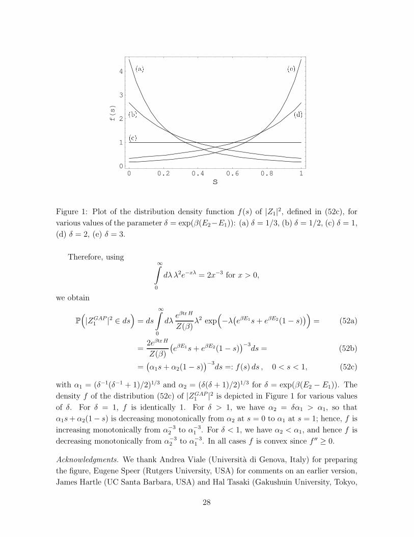
Figure 1: Plot of the distribution density function f(s) of |Z1|2, defined in (52c), for

various values of the parameter δ = exp(β(E2−E1)): (a) δ = 1/3, (b) δ = 1/2, (c) δ = 1,

(d) δ = 2, (e) δ = 3.

Therefore, using∞

∫

0

dλ λ2e−xλ = 2x−3 for x > 0,

we obtain

P

(

|ZGAP1 |2 ∈ ds

)

= ds

∞∫

0

dλeβtrH

Z(β)λ2 exp

(

−λ(

eβE1s+ eβE2(1 − s))

)

= (52a)

=2eβtrH

Z(β)

(

eβE1s+ eβE2(1 − s))−3

ds = (52b)

=(

α1s+ α2(1 − s))−3

ds =: f(s) ds , 0 < s < 1, (52c)

with α1 = (δ−1(δ−1 + 1)/2)1/3 and α2 = (δ(δ + 1)/2)1/3 for δ = exp(β(E2 − E1)). The

density f of the distribution (52c) of |ZGAP1 |2 is depicted in Figure 1 for various values

of δ. For δ = 1, f is identically 1. For δ > 1, we have α2 = δα1 > α1, so that

α1s+ α2(1− s) is decreasing monotonically from α2 at s = 0 to α1 at s = 1; hence, f is

increasing monotonically from α−32 to α−3

1 . For δ < 1, we have α2 < α1, and hence f is

decreasing monotonically from α−32 to α−3

1 . In all cases f is convex since f ′′ ≥ 0.

Acknowledgments. We thank Andrea Viale (Universita di Genova, Italy) for preparing

the figure, Eugene Speer (Rutgers University, USA) for comments on an earlier version,

James Hartle (UC Santa Barbara, USA) and Hal Tasaki (Gakushuin University, Tokyo,

28

Japan) for helpful comments and suggestions, Eric Carlen (Georgia Institute of Tech-

nology, USA), Detlef Durr (LMU Munchen, Germany), Raffaele Esposito (Universita di

L’Aquila, Italy), Rossana Marra (Universita di Roma “Tor Vergata”, Italy), and Her-

bert Spohn (TU Munchen, Germany) for suggesting references, and Juan Diego Urbina

(the Weizmann Institute, Rehovot, Israel) for bringing the connection between Gaus-

sian random wave models and quantum chaos to our attention. We are grateful for the

hospitality of the Institut des Hautes Etudes Scientifiques (Bures-sur-Yvette, France),

where part of the work on this paper was done.

The work of S. Goldstein was supported in part by NSF Grant DMS-0504504, and

that of J. Lebowitz by NSF Grant DMR 01-279-26 and AFOSR Grant AF 49620-01-

1-0154. The work of R. Tumulka was supported by INFN and by the European Com-

mission through its 6th Framework Programme “Structuring the European Research

Area” and the contract Nr. RITA-CT-2004-505493 for the provision of Transnational

Access implemented as Specific Support Action. The work of N. Zanghı was supported

by INFN.

References

[1] Aizenman, M., Goldstein, S., and Lebowitz, J. L.: On the stability of equilibrium

states of finite classical systems. J. Math. Phys. 16, 1284–1287 (1975).

[2] Arnol’d, V. I. and Avez, A.: Ergodic Problems of Classical Mechanics (Benjamin,

New York, 1968).

[3] Berry, M.: Regular and irregular eigenfunctions. J. Phys. A: Math. Gen. 10, 2083–

2091 (1977).

[4] Breuer, H.-P. and Petruccione, F.: Open Quantum Systems (Oxford University

Press, 2002).

[5] Brody, D. C. and Hughston, L. P.: The quantum canonical ensemble. J. Math.

Phys. 39, 6502–6508 (1998).

[6] Durr, D., Goldstein, S., and Zanghı, N.: Quantum equilibrium and the origin of

absolute uncertainty. J. Statist. Phys. 67, 843–907 (1992).

[7] Goldstein, S., Lebowitz, J. L., Tumulka, R., and Zanghı, N.: Canonical typicality.

In preparation.

[8] Goldstein, S., Lebowitz, J. L., Tumulka, R., and Zanghı, N.: Typicality of the GAP

measure. In preparation.

29

[9] Goldstein, S.: Stochastic mechanics and quantum theory. J. Statist. Phys. 47, 645–

667 (1987).

[10] Guerra, F. and Loffredo, M. I.: Thermal mixtures in stochastic mechanics. Lett.

Nuovo Cimento (2) 30, 81–87 (1981).

[11] Haag, R., Kastler, D., and Trych-Pohlmeyer, E. B.: Stability and equilibrium states.

Commun. Math. Phys. 38, 173–193 (1974).

[12] Hortikar, S. and Srednicki, M.: Correlations in chaotic eigenfunctions at large sep-

aration. Phys. Rev. Lett. 80(8), 1646–1649 (1998).

[13] Landau, L. D. and Lifshitz, E. M.: Statistical Physics. Volume 5 of Course of

Theoretical Physics. Translated from the Russian by E. Peierls and R. F. Peierls

(Pergamon, London and Paris, 1959).

[14] Lebowitz, J. L.: Boltzmann’s entropy and time’s arrow. Physics Today 46, 32–38

(1993).

[15] Lebowitz, J. L.: Microscopic reversibility and macroscopic behavior: physical ex-

planations and mathematical derivations. In 25 Years of Non-Equilibrium Statis-

tical Mechanics, Proceedings, Sitges Conference, Barcelona, Spain, 1994, in Lec-

ture Notes in Physics, J.J. Brey, J. Marro, J.M. Rubı, and M. San Miguel (eds.)

(Springer-Verlag, Berlin, 1995).

[16] Lebowitz, J. L.: Microscopic origins of irreversible macroscopic behavior. Physica

(Amsterdam) 263A, 516–527 (1999).

[17] Martin-Lof, A.: Statistical Mechanics and the Foundations of Thermodynamics.

Lecture Notes in Physics 101 (Springer, Berlin, 1979).

[18] Nelson, E.: Quantum Fluctuations (Princeton University Press, 1985).

[19] Page, D. N.: Average entropy of a subsystem. Phys. Rev. Lett. 71(9), 1291–1294

(1993).

[20] Schrodinger, E.: The exchange of energy according to wave mechanics. Annalen

der Physik (4), 83, 956–968 (1927).

[21] Schrodinger, E.: Statistical Thermodynamics. Second Edition (Cambridge Univer-

sity Press, 1952).

[22] Tasaki, H.: From Quantum dynamics to the canonical distribution: general picture

and a rigorous example. Phys. Rev. Lett. 80, 1373–1376 (1998).

30

[23] Urbina, J. D. and Richter, K.: Random wave models. Elsevier Encyclopedia of

Mathematical Physics (2006). To appear.

[24] von Neumann, J.: Beweis des Ergodensatzes und des H-Theorems in der neuen

Mechanik. Z. Physik 57, 30–70 (1929).

[25] von Neumann, J.: Mathematical Foundations of Quantum Mechanics (Princeton

University Press, Princeton, 1955). Translation of Mathematische Grundlagen der

Quantenmechanik (Springer-Verlag, Berlin, 1932).

[26] Walecka, J. D.: Fundamentals of Statistical Mechanics. Manuscript and Notes of

Felix Bloch (Stanford University Press, Stanford, CA, 1989).

31