On the asymptotic property analysis for a class of adaptive control systems with σ -modification

INTERNATIONAL JOURNAL OF ADAPTIVE CONTROL AND SIGNAL PROCESSINGInt. J. Adapt. Control Signal Process. (2012)Published online in Wiley Online Library (wileyonlinelibrary.com). DOI: 10.1002/acs.2334

On the asymptotic property analysis for a class of adaptive controlsystems with �-modification

Zhirong He1,2, Deqing Huang1,*,† and Jian-Xin Xu1

1Department of Electrical and Computer Engineering, National University of Singapore, Singapore 1175762Department of Mathematics, Sichuan University, Chengdu 610064, China

SUMMARY

With the effect of � -modification in adaptive control systems, robustness is achieved at the potential expenseof destroying some of the convergence properties. This paper proposes a qualitative analysis method for thesituations where the � -modification may lead to perfect tracking and also, given the prior knowledge of sys-tem parameters, may allow proper modification of the adaptive algorithm. The applicability of the proposedanalysis method is illustrated by two examples, where the system control gains that lead to global asymptoticconvergence are given explicitly. Further, simulations are performed to verify the qualitative analysis results.Copyright © 2012 John Wiley & Sons, Ltd.

Received 21 December 2011; Revised 15 August 2012; Accepted 18 August 2012

KEY WORDS: robust adaptive control; � -modification; global asymptotic convergence; Bendixon’scriterion

1. INTRODUCTION

Adaptive control (AC) has been exploited over 40 years with fruitful results [1,2]. The performanceof AC could be degraded in the presence of unmodeled dynamics, measurement noise, external dis-turbances, and improper robust gains [3–5]. Even when the original system is linear, fine controlperformance cannot be fully guaranteed, and the nonlinearity of the closed-loop system might resultin instability, everlasting oscillations, and so on. An illustrative example is the bursting phenomena[6], in which some peculiar oscillations may occur although the adaptive gain remains within thelimits of the so-called admissible domain. These oscillations vanish only when the designer is ableto detect a minimal value for the adaptive gain from prior knowledge. Therefore, the practical designof AC laws, especially robust AC (RAC) laws [7, 8], should be addressed more carefully.

Comparing with many other RAC schemes, in particular the projection [9] and dead-zone meth-ods [4, 7], the simple and nice Ioannou’s � -modification method [10] gives smoother parametricadaptation and does not require prior information on the control process, such as upper bound ofmodel error or unknown parameters [4, 7]. The robustness is achieved at the potential expense ofdestroying some of the convergence properties, that is, there is no more asymptotic convergenceand the fine tracking error is confined within a bounded region, specified by the modification gain� and the unknown parameters. To overcome the drawbacks of the � -modification scheme, severaladditional modifications have been suggested. For instance, in the switching � -modification scheme[7,10,11], the � -modification is switched off when the estimated parameters are below some accept-able bounds, where the bound information of the unknowns shall be available beforehand to designthe switching bounds. The �-modification [4] is another kind of revised � -modification, where the

*Correspondence to: Deqing Huang, Department of Electrical and Computer Engineering, National University ofSingapore, Singapore 117576.

†E-mail: [email protected]

Copyright © 2012 John Wiley & Sons, Ltd.

Z. HE, D. HUANG AND J.-X. XU

time-varying modification gain is proportional to the magnitude of tracking error. In consequence,the added robust part will be forced to zero in the case that the tracking error vanishes. The ratio-nale behind the �-modification is to retain the equilibrium at the point where the tracking errorand the parametric identification error become zero simultaneously. However, for those revised� -modification schemes, it is even harder to detect the asymptotic convergence of tracking errorusing the commonly used Lyapunov function-based analysis. This is because, in general, Lyapunovfunction-based method is not constructive.

In this work, instead of exploring more complicated robust adaptation schemes, we revisit thefundamental � -modification scheme and propose a qualitative analysis method for the situationswhere the � -modification may lead to perfect tracking and also, given the prior knowledge of systemparameters, may allow proper modification of the adaptive algorithm. First, we perform a Lyapunovanalysis for the RAC system, where the estimation of Lyapunov derivative reveals that the final ACperformance depends on the ultimate distance from the actual adaptive parameters and any set ofideal parameters. Then Bendixon’s criterion [12,13] is applied in the invariant set of state space thathas been derived by the Lyapunov analysis to detect the asymptotic convergence of the closed-loopsystem. We conclude that, by properly choosing the feedback gain and � -modification gain, globalasymptotic convergence of output tracking and parametric learning may still be achieved using thefundamental � -modification scheme. As such, more complex modification schemes, for example,the �-modification and the switching � -modification that are motivated as attempts to eliminatedrawbacks associated with the � -modification, are obviated. It is worth to highlight that the pro-posed analysis method relies on the existence of a Lyapunov function for a certain extended system[13]. Hence, it is still Lyapunov based whereas the Lyapunov function is not constructed directly.

The paper is organized as follows. Section 2 gives the AC design, without and with� -modification, for systems with parametric uncertainties. Section 3 performs Lyapunov analysisfor the closed-loop RAC systems with � -modification scheme, based on which a criterion is pro-posed to detect the asymptotic convergence of RAC. In the end, illustrative examples and theirsimulations are shown in Section 4.

2. AC DESIGN AND ITS � -MODIFICATION

In this section, we first revisit AC design for a class of linear-in-parameter system and then presentthe fundamental � -modification scheme.

2.1. AC design

Consider the following system [1, 7]

PxD f .x/C g.x/ŒuC!T.x/��, (2.1)

where g.x/ and f .x/ are smooth functions with f .0/ D 0, x 2 Rn is the system state, u 2 R isthe manipulated variable, !.x/ 2 Rl is a vector of known regressor, and � 2 Rl represents para-metric unknowns of the system. For the AC design of system (2.1), one may begin with a Lyapunovfunction for a nominal system (by dropping the unknown parameters �) of the form

PxD f .x/C g.x/u, (2.2)

which is uniformly asymptotically stabilizable at origin xD 0 by a continuously differentiable feed-back control law u D u0.x/ with u0.0/ D 0, and the corresponding control Lyapunov function(CLF) V0.x/ is known, satisfying [14]

c1kxk2 6 V0.x/6 c2kxk2, (2.3)

PV0.x/D@V0

@xŒf .x/C g.x/u0.x/�6 �c0kxk2, (2.4)

where ci , i D 0, � � � , 2 are some positive constants.

Copyright © 2012 John Wiley & Sons, Ltd. Int. J. Adapt. Control Signal Process. (2012)DOI: 10.1002/acs

ADAPTIVE CONTROL SYSTEMS WITH �-MODIFICATION

An additional feedback control part ur.x/ is designed using the knowledge of the CLF V0.x/ anduncertain parameter � such that the overall control

u.x/D u0.x/C ur.x/ (2.5)

stabilizes the actual system (2.1) in the presence of the uncertainty � . Substituting the control law(2.5) into (2.1) leads to the closed-loop system

PxD f .x/C g.x/u0.x/C g.x/�ur.x/C!T.x/�

�. (2.6)

Evaluating the derivative of V0.x/ along the trajectories of (2.6) gives

PV0.x/ D@V0

@xŒf .x/C g.x/u0.x/�C

@V0

@xg.x/

�ur.x/C!T.x/�

�6 �c0kxk2C

@V0

@xg.x/

�ur.x/C!T.x/�

�. (2.7)

The first term on the right-hand side of (2.7) is due to the nominal closed-loop system (2.4), andthe second term represents the effect of the control part ur.x/ and the uncertain term � on PV0.x/.Because of the matching condition, � appears exactly at the same point where ur.x/ appears. It ispossible to design ur.x/ to cancel the effect of � on PV0.x/ such that

@V0

@xg.x/Œur.x/C!T.x/��6 0.

Considering that the uncertain term in (2.1) is linear-in-parameter, AC techniques can be conve-niently used to achieve both the closed-loop asymptotic stability and a smooth control law. If � wasknown, the control law u D u0 � !

T.x/� would directly cancel the term associated with � , andrender to PV 6 �c0kxk2, as can be seen from (2.7).

When � is unknown, define the certainty-equivalence control law

u.x/D u0.x/�!T.x/ O� , (2.8)

where O� represents the estimate of unknown � . Substituting (2.8) into (2.1) leads to the closed-loopsystem

PxD f .x/C g.x/�u0.x/C!T.x/ Q�

�, Q� , � � O� . (2.9)

Consider the Lyapunov function candidate by augmenting V0.x/ with a quadratic parameterestimation error term as follows

V.x, Q�/D V0.x/C1

2Q�T��1 Q� , � D �T > 0. (2.10)

Noting that PQ� D�PO� , the time derivative of V.x, Q�/ along system (2.9) is

PV .x, Q�/ D@V0

@xŒf .x/C g.x/u0.x/C g.x/!T.x/ Q��C Q�

T��1PQ�

D@V0

@xŒf .x/C g.x/u0.x/�C Q�

T��1

��!.x/

@V0

@xg.x/� PO�

�.

Apparently, choosing the parameters adaptation algorithm as

PO� D �!.x/@V0

@xg.x/ (2.11)

yields

PV .x, Q�/D@V0

@xŒf .x/C g.x/u0.x/�6 �c0kxk2. (2.12)



In (2.11), the unknown parameter � is identified by just integrating the state-relevant function�!.x/ @V0

@x g.x/. As a result, the possible unmodeled dynamics or external disturbances may result inparameter drift, which is undesirable and dangerous to real implementation. � -modification is thusproposed to enhance the robustness of AC systems.

2.2. The � -modification scheme

The parametric updating law (2.11) is modified as [10, 11]

PO� D��O� � �0

�C �!.x/

@V0

@xg.x/, (2.13)

where � 2R is a positive tuning parameter, � is the adaptation gain specified in (2.10), and �0 is avector design parameter that is often selected to be zero, unless there is better prior information about

the value of � . It can be seen from (2.13) that the additional term ��O� � �0

�prevents O� from

drifting to infinity by pulling it toward �0. Intuitively, if because of nonzero !.x/ @V0@x g.x/ the param-

eter estimate O� starts drifting to large positive values, then the added negative term ��O� � �0

�becomes large in magnitude, thus forcing the parameter estimate to decrease.

Without loss of generality, assume �0 D 0 in the consequent analysis. By combining (2.1) and(2.13), the new closed-loop system is(

PxD f .x/C g.x/Œu0C!T.x/ Q��,PO� D�� O� C �!.x/ @V0

@x g.x/.(2.14)

With the effect of � -modification in the AC law (2.13), asymptotic tracking convergence cannot beguaranteed for the closed-loop system (2.14) using the Lyapunov function (2.10). The state x andthe parametric adaptation error Q� can only be proven to stay in a bounded region ultimately specifiedby the coefficient � and the unknown parameter � . More concretely, noticing (2.12) and Q� D �� O� ,

PV .x, Q�/ D@V0

@xŒf .x/C g.x/u0.x/�C � Q�

T O�

6 �c0kxk2 �1

2� Q�

T Q� C1

2� Q�

T Q� C � Q�T O�

D �c0kxk2 �1

2� Q�

T Q� C1

2� Q�

T Q� C1

2� Q�

T O� C1

2� O�

T Q� C1

2� O�

T O� �1

2� O�

T O�

D �c0kxk2 �1

2� Q�

T Q� C1

2��T� �

1

2� O�

T O� . (2.15)

Omitting the last minus term on the right-hand side of (2.15), we obtain

PV .x, Q�/6 �c0kxk2 �1

2� Q�

T Q� C1

2��T� .

Thus, if

c0kxk2C1

2� Q�

T Q� >1

2��T� ,

we have PV .x, Q�/ < 0. Define

D0 D��

xT, O�T�T2RnCl j c0kxk2C

1

2� Q�

T Q� 6 12��T�

. (2.16)

As PV .x, Q�/ < 0 as�

xT, O�T�T… D0, any trajectory of (2.14) that starts from the outside of D0

will go into D0 as t increases. Hence, D0 is an invariant set of (2.14). Moreover, it is easy to see thatD0 is compact, bounded closed in RnCl . For different values of � , D0 changes its size and location,but keeps the spherical shape.



Remark 1The aforementioned analysis reveals that the specific choice of Lyapunov function, namely (2.10),does not allow us to conclude on asymptotical stability of (2.14). The final AC performance dependson the ultimate distance from the actual adaptive parameters and any set of ideal parameters.

In order to explore the possibility of asymptotic convergence by using the fundamental� -modification (2.13), dynamic analysis of (2.14) in the domain D0 becomes indispensable.

3. GLOBAL ASYMPTOTICAL CONVERGENCE OF RAC WITH � -MODIFICATION

To analyze the tendency of the trajectories of the closed-loop system (2.14) in the domain D0,the following notations and preliminary results on qualitative analysis of differential equations arebriefly introduced.

3.1. Preliminary

Consider the following autonomous differential equation

PXD F.X/, (3.1)

where X 2 Rm and F 2 C 1.Rm,Rm/. Let U D B2.0, 1/ be the Euclidean unit ball in R2, andNU , @U the closure and boundary of U , respectively. Define a set Lip.M1 ! M2/ D f� W M1 7!M2j � is Lipschitz continuousg, where Mi , i D 1, 2 are the subsets of certain metric spaces. ForD � Rm, a function ' 2 Lip. NU ! D/ is described as a simply connected rectifiable surface inD, and a function 2 Lip.@U ! D/ is described as a closed rectifiable curve in D. Moreover, if D '.@U /, we say D @'. If D is an open, simply connected set, then

†. ,D/, f' 2 Lip. NU !D/j'.@U /D .@U /g

is non-empty for each simple closed rectifiable curve in D. Let D1 �Rm be the domain of F in(3.1). Consider functionals S on the surfaces Lip. NU !D1/ of the form

S ' D

ZNU

S

'.u/,

@

@u1'.u/^

@

@u2'.u/

�du, (3.2)

where u D .u1,u2/ 2 NU � R2, .X, Y/ 7! S.X, Y/ is a real valued function with X 2 D1 � Rm,Y 2RM , M Dm.m� 1/=2, and f1.t/^ f2.t/ denotes the Grassman product (exterior product) off1 and f2. A general class of function S that interests us is S.X, Y/ D jA.X/Yj, where j � j is anynorm on RM , and X 7! A.X/ is a C 1 nonsingular real M �M matrix-valued function.

Further, introduce several matrix-related definitions. Let � be the Lozinskii logarithmic norm ofthe matrix B [15, pp. 41], that is,

�.B/D limh!0C

jI C�Bj � 1

h. (3.3)

�.B/ can also be calculated as follows,

�.B/D supi

.<.bi i /C†j ,j¤i jbij j/, (3.4)

where bij represents the element on the i th row and j th column of B , and <.bi i / refers to the realpart of bi i . For a m �m matrix D, denote DŒ2� 2 RM�M as the second additive compound of D.The details on the definition ofDŒ2� can be seen from [16]. Moreover, a subset D of D0 is positivelyinvariant with respect to (3.1) if X.t ,D/DD for all t 2 Œ0,1/. A simple closed rectifiable curve in D0 is invariant with respect to (3.1) if .@U / is invariant with respect to (3.1). We say that thedomain D1 has the minimum property with respect to S if, for each simple closed rectifiable curve in D1, there is a minimizing sequence 'q 2 †. ,D1/ for S such that

Sq '

q. NU / has compactclosure in D1.

The following Bendixon’s criterion [12] is important for us to derive the main result of this paper.



Lemma 1Suppose that (a) D1 has the minimum property with respect to S.X, Y/ D jA.X/Yj, and that (b)

�

@A@XFA

�1CA�@F@X

�Œ2�A�1

�< 0 on D1. Then there are no simple closed rectifiable curves in

D1 that are invariant with respect to (3.1).

Consider a special case S.X, Y/D jYj, and we have the following.

Theorem 1Suppose that (a) D1 has the minimum property with respect to S.X, Y/ D jYj, and that (b)

�

�@F@X

�Œ2��< 0 on D1. Then there are no simple closed rectifiable curves in D1 that are invariant

with respect to (2.14).

ProofAs S.X, Y/ D jA.X/Yj D jYj, the matrix-value function A.X/ is an identity matrix. Conse-

quently, �

@A@XFA

�1CA�@F@X

�Œ2�A�1

�D �

�@F@X

�Œ2��. Hence, Theorem 1 is directly implied

by Lemma 1. �

Remark 2In Theorem 1, a special choice of matrix A is considered only. Such choice facilitates the calcula-tion of norm � and the adjacent qualitative analysis of RAC system. As a result, the gain conditionwe derive later to ensure the asymptotic convergence of RAC system is only a sufficient condition.Other choices of A would yield other sufficient conditions for the control gains to achieve asymp-totic convergence. For the considered RAC system, if the simplest choice of A cannot yield anyfeasible design of control gains, more complex A should be tried as alternatives.

On the basis of Theorem 1, a criterion is proposed in the following to detect the global asymptoticconvergence of the RAC system (2.14).

3.2. A criterion on global asymptotic convergence

Global asymptotic convergence of the closed-loop system (2.14) refers to that the state variableX, ŒxT,�T�T, no matter what the initial value of state is, will converge to the desired state asymp-totically as t !1. This reveals that a pre-condition to achieve the global asymptotic convergencefor (2.14) is that the desired state is the unique equilibrium of (2.14). Without loss of generality,consider the regulation problem for (2.14) only. Then the following assumption will validate ourfollowing analysis.

Assumption 1System (2.14) has a single (locally) stable equilibrium E W .0, 0/ 2D0, where D0 is given in (2.16).

Recall that the domain D0 is a positively invariant set of (2.14), and all trajectories starting fromthe outside of D0 will converge to D0 as t increases. Hence, if the unique equilibrium E in D0 isasymptotically stable with respect to D0, E is globally asymptotic stable in the whole state place.Calculate the Jacobian matrix of system (2.14), and it yields

@F

@XDD D

0@ @

@xf .x/C@@XŒg.x/u0�C @

@X

�g.x/!T.x/

�Q� g.x/!T.x/

@@x

h�!.x/ @V0.x/

@x g.x/i

��

1A .



Theorem 2Consider system (2.14) and assume that Assumption 1 is satisfied. If, for any D1 � D0, where D0is defined in (2.16), the conditions (a) and (b) in Theorem 1 are satisfied, then the equilibrium E isglobally asymptotic stable.

ProofUnder the conditions (a) and (b), by Theorem 1, there are no simple closed rectifiable curves in D1.Owing to the relationship D1 � D0, there are no simple closed rectifiable curves in D0. Thus, the!-limit set [17,18] of any trajectory of (2.14) in D0 can only be fixed points. Noticing that the equi-librium E is the single fixed point in D0 and stable, any trajectory starting from D0 will convergeto E as t ! C1. Furthermore, as D0 is a positively invariant set of (2.14), the equilibrium E isglobally asymptotic stable. The proof is complete. �

4. ILLUSTRATIVE EXAMPLES WITH ANALYSIS AND DESIGN

To demonstrate the efficacy of the proposed analysis method in detecting the global asymptoticconvergence of RAC under the fundamental � -modification, we first consider the state regulationproblem of the following system �

Px D�axC y,Py D bxC cy C u,

(4.1)

where a > 0, c ¤ 0 are known and b is a constant parametric uncertainty. Writing (4.1) into theform of system (2.1), we have xD .x,y/T 2R2, and

f .x/D�axC ycy

�, g.x/D

0

1

�, !.x/D x, � D b.

Using the Lyapunov function-based AC design technique, the robust adaptive controller with� -modification is given as follows,

uD��ObC 1

�x � ky,

POb D�� ObC xy, Ob.0/D 0, (4.2)

where k > c is the feedback gain and � > 0 is the � -modification gain. Substituting (4.2) into (4.1)yields the closed-loop system 8̂<

:̂Px D�axC y,Py D .b � 1/xC .c � k/y � x Ob,POb D�� ObC xy.

(4.3)

Remark 3It can be seen from (4.3) that the closed-loop correspondence of the linear system (4.1) has becomea nonlinear system. It presents extremely complex nonlinear dynamic behaviors and is more genericthan the Lorenz equation [19], which is well known for its rich and complex behaviors such asbifurcations and singular attractors. Hence, it is necessary for us to provide Theorems 3 and 4 withqualitative analysis to disclose the inherent relationship between the RAC gains and the globalasymptotic convergence of (4.3).

System (4.3) has three possible equilibria, which are denoted by

E1 W .0, 0, 0/ and E˙ W

xe , axe ,

ax2e�

�, xe ,˙

r�Œa.c � k/C b � 1�

a. (4.4)

It is easy to see that (4.3) has only one equilibrium E1 if and only if

a.c � k/C b � 16 0, (4.5)



and three distinct equilibria E1 and E˙ otherwise. Both E� and EC are in the upper half-spacef.x,y, Ob/ 2R3j Ob > 0g and symmetric with respect to the Ob-axis.

4.1. Lyapunov function-based analysis

To explore the dynamic behavior of system (4.3) in the whole state space, we first conduct theLyapunov function-based analysis. Choose the Lyapunov function as follows,

V�x,y, Ob

�D1

2x2C

1

2y2C

1

2

�b � Ob

�2. (4.6)

Differentiating (4.6) and substituting the closed-loop dynamics (4.3) lead to

PV�x,y, Ob

�D x PxC y Py �

�b � Ob

�POb

D x.�axC y/C yh.b � 1/x � x ObC .c � k/y

i��b � Ob

� �� ObC xy

�D �ax2C .c � k/y2C � Ob.b � Ob/

6 �ax2C .c � k/y2 ��

2

�Ob � b

�2C�

2b2,

which renders to

PV�x,y, Ob

�6 ��

1

2x2C

1

2y2C

1

2

�Ob � b

�2�C ı D��V C ı (4.7)

with � Dminf2a, 2.k � c/, �g, ı D �b2=2. The inequality (4.7) implies that the solution of (4.7) isupper bounded by the solution of equation PV0 D��V0C ı, that is,

V0.t/D V0.0/e��t C

ı

�.1� e��t /.

As such, as t !C1,

V.t/D1

2x2C

1

2y2C

1

2

�Ob � b

�26 ı

�D

�b2

2minf2a, 2.k � c/, �g.

Define

D0 D��x,y, Ob

�2R3j

1

2x2C

1

2y2C

1

2

�Ob � b

�26 ı

�D

�b2

2minf2a, 2.k � c/, �g

. (4.8)

Any trajectory of (4.3) will go into the domain D0 as t ! C1 and no longer depart from D0.Hence, D0 is a positively invariant set of (4.3). Dynamic analysis of (4.3) within D0 is presented inthe following part.

4.2. Uniqueness of equilibrium and its global asymptotic convergence

To analyze the qualitative properties of the system (4.3) in D0, the first step is to conduct localstability analysis for each equilibrium. However, because of the global asymptotic convergenceconcern for the equilibrium E1 only, we assume that E˙ vanishes or does not exist. Equivalently,the condition a.c � k/C b � 16 0 holds by (4.5).

At the equilibrium E1.0, 0, 0/, the Jacobian is

JE1 D@F

@X.0, 0, 0/D

24 �a 1 0

b � 1 c � k 0

0 0 ��

35 . (4.9)

The characteristic polynomial of the Jacobian matrix (4.9), evaluated at the equilibrium E1, isgiven by

det.I � JE1/D .C �/Œ2C .a� .c � k//� .a.c � k/C b � 1/�, (4.10)



which determines the eigenvalues of JE1

1 D�� < 0,2,3 D�a� .c � k/

2˙1

2

p.a� .c � k//2C 4.a.c � k/C b � 1/. (4.11)

As 1 is always negative, the stability of E1 is determined by the signs of <f2,3g.

Theorem 3Let W0 D f.a, b, c � k, �/ 2 R4ja.c � k/ C b � 1 6 0g. Consider system (4.3), for all.a, b, c � k, �/ 2W0, the single equilibrium E1.0, 0, 0/ is locally stable.

ProofConsider the following three different scenarios.

C1: a.c � k/C b � 1 < �14.a� .c � k//2. The eigenvalues 2,3 are a pair of conjugate complex

numbers with <f2,3g D �a�.c�k/

2< 0. The equilibrium E1 is stable.

C2: �14.a � .c � k//2 6 a.c � k/C b � 1 < 0. 2,3 satisfy 2 6 3 < 0. The equilibrium E1 is

stable.C3: a.c � k/C b � 1 D 0. We have that 2 D �.a � .c � k// < 0 and 3 D 0. Thus, E1 is

degenerate in this case. Introduce a state transformation: x1 D�.c�k/xCy, y1 D�axCy,with which (4.3) is changed to8̂̂

<ˆ̂:Px1 D�

x1�y1a�.c�k/

Ob,

Py1 D�.a� .c � k//y1 �x1�y1a�.c�k/

Ob,POb D�� ObC x1�y1

a�.c�k/

ha.x1�y1/a�.c�k/

C y1

i.

(4.12)

Apply the center manifold theory [17] and solve Py1 D 0, POb D 0 in the neighborhood of E1,

y1 D g1.x1/D�a

�.a�.c�k//4x31 CO

�x51

,

Ob D g2.x1/Da

�.a�.c�k//2x21 CO

�x41

,

where O�xn1

denotes all terms with order > n. Then, by substituting y1 D g1.x1/ andOb D g2.x1/ into the first equation of (4.12), the flow on the center manifold can be expressedas

Px1 D�1

a� .c � k/.x1 � g1.x1//g2.x1/D�

a

�.a� .c � k//3x31 CO

�x51

,

implying that the equilibrium E1 is stable.

Thus, noticing thatW0 DS3iD1 Ci , the single equilibrium E1 is locally stable for all .a, b, c�k, �/

2W0. �

Next, by applying Theorem 2, we derive sufficient conditions to guarantee the global stability ofE1. As a consequence, (4.3) achieves global asymptotic convergence under the same conditions.

Theorem 4Define

W1 D

�.a, b, c � k, �/ 2R4jmin

�� C k � c � 1� "

p2

, aC k � c � ", aC � � 1� "

> jbjmax

�r�

2a,r

�

2.k�c/, 1

.

where " > 0 is a sufficiently small constant. Consider system (4.3) with k > 0 and � > 0

being tunable control gains. For .a, b, c � k, �/ 2 W0TW1, the unique equilibrium E1.0, 0, 0/ is

globally stable.



ProofConsider (4.3) with the system state X D .x,y, Ob/T. For .a, b, c � k, �/ 2 W0, the unique equilib-rium E1 is locally stable by Theorem 3. As D0 has been proven to be a positively invariant set ofsystem (4.3), it suffices to derive the asymptotic stability of E1 in D0 only. To apply Theorem 2,the main steps are to construct a new set D1 such that D0 � D1, and prove that D1 satisfies theconditions (a) and (b) in Theorem 1.

First, construct the domain D1 and check the condition (b). The Jacobian matrix D of (4.3) andits second additive compound DŒ2� are

D D@F

@XD

24 �a 1 0

b � 1� Ob c � k �xy x ��

35 , DŒ2� D

24 �aC c � k �x 0

x �a� � 1

�y b � 1� Ob c � k � �

35 .

In this case, M D 3 and Y 2 R3 in (3.2). The norm of vector Y is defined as jYj D

sup

�qy21 C y

22 , jy3j

. By the definition of �.B/ in (3.3) and its equivalent computation in (3.4),

we have

��DŒ2�

�D sup

jD1,�� ,3f<.di i /C†j ,j¤i jdij j/g

D supf�aC c � kC jxj,�a� � C 1C jxj,

jyj C j Ob � bC 1j C c � k � �g, (4.13)

where dij represents the element on the i th row and j th column of DŒ2�. Let

D1 Dn.x,y, Ob/ 2R3jjxj6minfaC k � c, aC � � 1g � ",

jyj C j Ob � bC 1j6 � C k � c � "o

,

where c � k < 0, a > 0, � > 0, and " is the same as in W1. If .x,y, Ob/ 2 D1, we have �.DŒ2�/ < 0

by (3.4) and (4.13). As such, the condition (b) in Theorem 1 is satisfied.Furthermore, check the condition (a). Assume that S.X, Y/ D jYj. For any '.u/ , .'1.u/,

'2.u/,'3.u// 2 Lip. NU ,D1/, the functional S ' in (3.2) is

S ' D

ZNU

ˇ̌̌ˇ @@u1'.u/^

@

@u2'.u/

ˇ̌̌ˇdu

D

ZNU

ˇ̌̌ˇ@.'2,'3/

@.u1,u2/,@.'3,'1/

@.u1,u2/,@.'1,'2/

@.u1,u2/

�ˇ̌̌ˇ du

D

ZNU

sup

8<:�@.'2,'3/2

@.u1,u2/C@.'3,'1/2

@.u1,u2/

� 12

,

ˇ̌̌ˇ@.'1,'2/

@.u1,u2/

ˇ̌̌ˇ9=; du. (4.14)

We state that D1 has the minimum property with respect to S , that is, for each simple closed recti-fiable curve 2 D1, there is a minimizing sequence f'qg � †. ,D1/ for S such that

Sq '

q. NU /has compact closure in D1. If there exists a minimizing sequence f'qg � †. ,D1/ for S , thecompact closeness property of

Sq '

q. NU / is directly obtained because of the boundedness of D1.Thus, it suffices to find a sequence f'qg � D1 such that f'qg � †. ,D1/ and it is minimizingfor S . For each simple closed rectifiable curve 2 D1, it is easy to find a minimizing sequencef'qg � †. ,R3/ for S . Our next aim is to construct a new minimizing sequence f Q'qg such thatf Q'qg �†. ,D1/ for S , by modifying f'qg.

To address this, denote c1 D � C k � c � " and k1 D minfa C k � � , a C � � 1g � ". Theboundary of D1 is determined by the following six planes, …1˙ W ˙.y C . Ob � b C 1// D c1,…2˙ W ˙.y � . Ob � b C 1// D c1, and …3˙ W ˙x D k1. As such, there are six half-spaces:G1˙ W ˙.yC . Ob�bC1//6 c1, G2˙ W ˙.y� . Ob�bC1//6 c1, and G3˙ W ˙x 6 k1 that all contain



D1 as their subset. If there exists ' in f'qg that crosses any one of the six planes, we need to modify' to derive Q'. Without loss of generality, consider the plane …1C and its corresponding half-spaceG1C, and suppose that '.u/j NU D .'1.u/,'2.u/,'3.u//j NU crosses the plane …1C. Then there existsU0 � NU such that '2.u/C .'3.u/� bC 1/ > c1 if u 2 U0. Define Q' by modifying ' as follows,�

Q'.u/D '.u/, if u 2 U nU0,Q'1.u/D '1.u/, Q'2.u/D c1C b � 1� '3.u/, Q'3.u/D c1 � '2.u/, if u 2 U0.

It is easy to see that Q' 2†. ,G1C/ and Q' does not cross…1C. Furthermore, S Q' DS ' by (4.14).After defining Q' similarly in the other five scenarios, the new sequence f Q'qg can be constructedsuch that f Q'qg �

T3iD1Gi˙ DD1, and S Q' DS ', whereas it does not cross any of the six planes.

As a result, f Q'qg is a minimizing sequence in †. ,D1/ for S . Therefore, there is a compact boxin D1 that contains the curve and a minimizing sequence f Q'qg for S in †. ,D1/. By defini-tion, D1 has the minimum property with respect to S.X, Y/ D jYj. This proves the condition (a)in Theorem 1.

Notice that the uniqueness and local stability condition for E1.0, 0, 0/ is .a, b, c�k, �/ 2W0. ByTheorem 2, E1 is globally stable if .a, b, c�k, �/ 2W0 and D0 �D1. As D0 �D1 is equivalent to.a, b, c�k, �/ 2W1,E1 is globally stable as .a, b, c�k, �/ 2W0

TW1. The proof is complete. �

Remark 4In Theorem 4, sufficient parametric condition is derived for the closed-loop system (4.3) to ensurethe global stability of the unique equilibrium E1 and thus the perfect state regulation. By theLyapunov function analysis, the bounded absorbing closed set D0 is first constructed in the statespace. It is worth noticing that the definition of D0 does not put any constraints between systemparameters and control gains, and it is hard, if not impossible, to prove that there are no simpleclosed rectifiable curves in D0 under random parametric conditions. Alternatively, we claim this inD1, another subset of the state space. Then, the parametric condition, derived by solving D0 � D1,just provides the constraints of parameters under which there are no simple closed rectifiable curvesin D0.

The non-empty property of W0TW1 depends on the system parameters a, b, c, and the control

gains k and � . Given the values of a and c as well as the prior information of b, properly choosingk and � might lead to a non-empty W0

TW1, as demonstrated in the following simulations.

4.3. Simulation results

Three simulations are conducted in the following. The first one is to show the asymptoticconvergence of trajectories of system (4.3) without � -modification.

The second one is to show the variations of trajectory under the effect of � -modification. System(4.3) may lose its asymptotic stability when the feedback gain k and the modification gain � arenot well designed. The last one is to show that after redesigning the parameters k and � , the globalasymptotic convergence of system (4.3) is recovered.

Randomly choose six different initial points: A1D .4, 3, 10/, A2D .2,�3, 3/, A3D .4,�4,�3/,A4D.�2,�3,�5/,A5D.�2,�3, 3/ andA6 D .�3, 6, 1/. In system (4.1), without loss of generality,assume a D 2, b D 10, and c D 4. Because of parametric uncertainty, the available information forb is that b 2 Œ�13, 13� when considering the AC design for (4.1).

Simulation 1: Without � -modification of parametric adaptation, the closed-loop system (4.3) is8̂<:̂Px D�axC y,Py D .b � 1/xC .c � k/y � x Ob,POb D xy.

(4.15)

Choose the Lyapunov function V.x,y, Ob/ as in (4.6), and one has PV D �ax2 C .c � k/y2. Letk D 8 such that k > c, system (4.15) is globally stable. The system trajectories starting from points



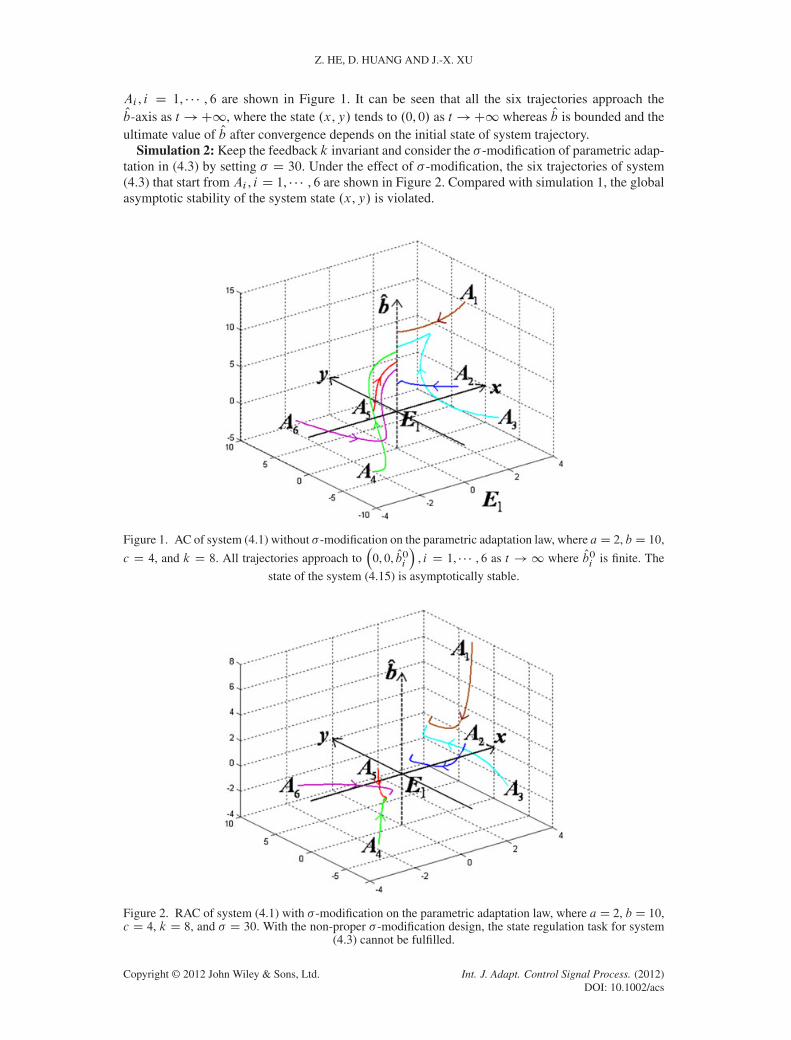
Ai , i D 1, � � � , 6 are shown in Figure 1. It can be seen that all the six trajectories approach theOb-axis as t !C1, where the state .x,y/ tends to .0, 0/ as t !C1 whereas Ob is bounded and theultimate value of Ob after convergence depends on the initial state of system trajectory.

Simulation 2: Keep the feedback k invariant and consider the � -modification of parametric adap-tation in (4.3) by setting � D 30. Under the effect of � -modification, the six trajectories of system(4.3) that start from Ai , i D 1, � � � , 6 are shown in Figure 2. Compared with simulation 1, the globalasymptotic stability of the system state .x,y/ is violated.

Figure 1. AC of system (4.1) without � -modification on the parametric adaptation law, where aD 2, b D 10,

c D 4, and k D 8. All trajectories approach to�0, 0, Ob0

i

�, i D 1, � � � , 6 as t ! 1 where Ob0

iis finite. The

state of the system (4.15) is asymptotically stable.

Figure 2. RAC of system (4.1) with � -modification on the parametric adaptation law, where aD 2, b D 10,c D 4, k D 8, and � D 30. With the non-proper � -modification design, the state regulation task for system

(4.3) cannot be fulfilled.



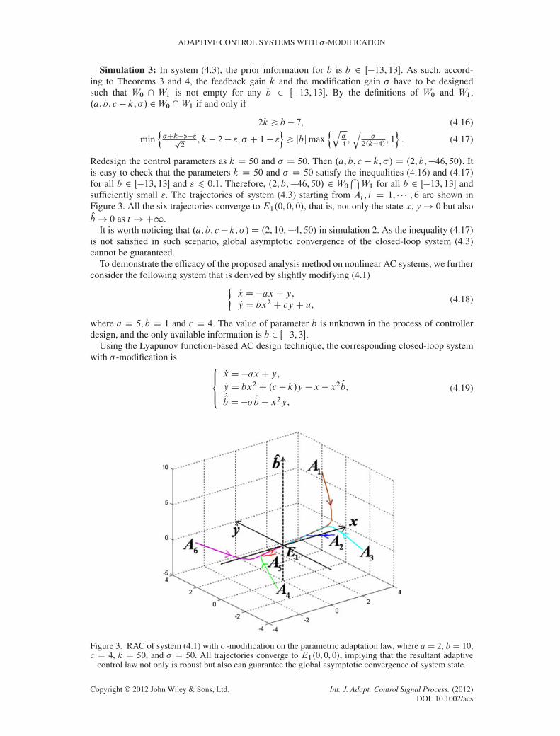
Simulation 3: In system (4.3), the prior information for b is b 2 Œ�13, 13�. As such, accord-ing to Theorems 3 and 4, the feedback gain k and the modification gain � have to be designedsuch that W0 \ W1 is not empty for any b 2 Œ�13, 13�. By the definitions of W0 and W1,.a, b, c � k, �/ 2W0 \W1 if and only if

2k > b � 7, (4.16)

minn�Ck�5�"p

2, k � 2� ", � C 1� "

o> jbjmax

nq�4

,q

�2.k�4/

, 1o

. (4.17)

Redesign the control parameters as k D 50 and � D 50. Then .a, b, c � k, �/ D .2, b,�46, 50/. Itis easy to check that the parameters k D 50 and � D 50 satisfy the inequalities (4.16) and (4.17)for all b 2 Œ�13, 13� and " 6 0.1. Therefore, .2, b,�46, 50/ 2 W0

TW1 for all b 2 Œ�13, 13� and

sufficiently small ". The trajectories of system (4.3) starting from Ai , i D 1, � � � , 6 are shown inFigure 3. All the six trajectories converge to E1.0, 0, 0/, that is, not only the state x,y! 0 but alsoOb! 0 as t !C1.

It is worth noticing that .a, b, c � k, �/D .2, 10,�4, 50/ in simulation 2. As the inequality (4.17)is not satisfied in such scenario, global asymptotic convergence of the closed-loop system (4.3)cannot be guaranteed.

To demonstrate the efficacy of the proposed analysis method on nonlinear AC systems, we furtherconsider the following system that is derived by slightly modifying (4.1)�

Px D�axC y,Py D bx2C cy C u,

(4.18)

where a D 5, b D 1 and c D 4. The value of parameter b is unknown in the process of controllerdesign, and the only available information is b 2 Œ�3, 3�.

Using the Lyapunov function-based AC design technique, the corresponding closed-loop systemwith � -modification is 8̂<

:̂Px D�axC y,Py D bx2C .c � k/y � x � x2 Ob,POb D�� ObC x2y,

(4.19)

Figure 3. RAC of system (4.1) with � -modification on the parametric adaptation law, where aD 2, b D 10,c D 4, k D 50, and � D 50. All trajectories converge to E1.0, 0, 0/, implying that the resultant adaptive

control law not only is robust but also can guarantee the global asymptotic convergence of system state.



where c � k < 0. Performing a similar analysis as we did for the first example, correspondingly,we have

W0D

�.a, b, c�k, �/ 2R4j

3

8a

3p2a2�4

3pb4C�.ac�ak�1/ < 0

, (4.20)

W1 D˚.a, b, c � k, �/ 2R4j

min

8<:paCk�c�",

pajC��1�",

sp2jc�k�� C 1j

2�",

sp2jc�k�� 1j

2�"

9=;

> jbjmax

�r�

2a,r

�

2.k�c/, 1

, (4.21)

D0D�.x,y, Ob/ 2R3j

1

2x2C

1

2y2C

1

2. Ob�b/2 6 ı

�D

�b2

2minf2a, 2.k�c/, �g

, (4.22)

D1Dn.x,y, Ob/ 2R3jx2 6minfaCk � c, aC� � 1g�",

j2xyjCj2x. Ob�b/C1j6 �Ck�c�"o

. (4.23)

If .a, b, c � k, �/ 2 W0, system (4.19) has only one equilibrium E1.0, 0, 0/, which is in thepositively invariant set D0. Further, there are no simple closed curves in D1. In addition, if.a, b, c�k, �/ 2W0

TW1, then D0 �D1. In consequence, in order to guarantee the global asymp-

totic convergence of the closed-loop system (4.19), the feedback gain k and the modification gain� have to be designed such that W0 \W1 is non-empty for any b 2 Œ�3, 3�. By (4.20) and (4.21),.a, b, c � k, �/ 2W0 \W1 if and only if

jbj<4

3

4

r15

�

4p.5k � 9/3, (4.24)

min

8<:pkC 1� ",

p� C 4� ",

sp2 jkC � � 5j

2� ",

sp2 jkC � � 3j

2� "

9=;>

> jbjmax

�r�

10,r

�

2.k � 4/, 1

. (4.25)

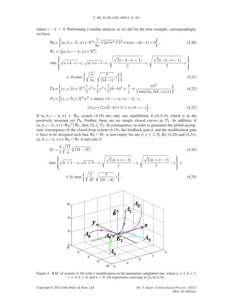
Figure 4. RAC of system (4.18) with � -modification on the parametric adaptation law, where aD 5, b D 1,c D 4, k D 9, and � D 9. All trajectories converge to E1.0, 0, 0/.



Let k D 9, � D 9, and it is easy to check that (4.24) and (4.25) hold for all b 2 Œ�3, 3� and" 6 0.01. Therefore, .a, b, c � k, �/ D .5, b,�5, 9/ 2 W0

TW1 for all b 2 Œ�3, 3� and suf-

ficiently small ". Randomly choose six different initial points: A1 D .2, 3, 8/, A2 D .4, 3, 10/,A3 D .4,�3,�3/, A4 D .�2,�3,�5/, A5 D .�2,�3, 3/, and A6 D .�3, 6, 1/. The trajectories ofsystem (4.19) starting from Ai , i D 1, � � � , 6 are shown in Figure 4. All the six trajectories convergeto E1.0, 0, 0/ asymptotically, that is, not only the state x,y! 0 but also Ob! 0 as t !C1.

5. CONCLUSION

This paper presents an analysis method to detect the global asymptotic convergence of AC sys-tems with robust � -modification. Although the � -modification does eliminate the danger of totaldivergence and instead guarantees that all values of the closed-loop system remain bounded, theyare usually achieved at the expense of destroying some of the convergence properties. The quali-tative analysis result reveals that even with the � -modification scheme, by properly designing thefeedback gain and the modification gain, global asymptotic convergence can still be achieved incertain situations.

This has been properly demonstrated by examples and their simulations.

REFERENCES

1. Astrom KJ, Wittenmark B. Adaptive Control, (2nd edn). Addison-Wesley Publishing Company: Boston, MA, 1995.2. Fekri S, Athans M, Pascoal A. Issues, progress and new results in robust adaptive control. International Journal of

Adaptive Control and Signal Processing 2006; 20(10):519–579.3. Barkana I. Gain conditions and convergence of simple adaptive control. International Journal of Adaptive Control

and Signal Processing 2005; 19(1):13–40.4. Farrell JA, Polycarpou MM. Adaptive Approximation Based Control-Unifying Neural, Fuzzy and Traditional

Adaptive Approximation Approaches. John Wiley & Sons: Hoboken, New Jersey, 2006.5. Yang C, Ma H. Adaptive predictive control of time-varying NARMA systems with exact output tracking. In

Proceedings of the 30th Chinese Control Conference (CCC), Yantai, 2011; 2515–2520.6. Kaufman H, Barkana I, Sobel K. Direct Adaptive Control Algorithms, (2nd edn). Springer Verlag: New York, 1997.7. Ioannou PA, Sun J. Robust Adaptive Control. Prentice Hall: Upper Saddle River, NJ, 1996.8. Zhao Q, Pan Z, Fernandez E. Reduced-order robust adaptive control design of uncertain SISO linear systems.

International Journal of Adaptive Control and Signal Processing 2008; 22(7):663–704.9. Wang LX. Stable adaptive fuzzy control of nonlinear systems. IEEE Transactions on Fuzzy Systems 1993; 1:146–155.

10. Ioannou PA, Kokotovic PV. Adaptive Systems With Reduced Models. Springer-Verlag: New York, 1983.11. Tsakalis KS. The �-modification in the adaptive control of linear time-varying plants. In Proceedings of the 31st

Conference on Decision and Control, Tucson, Arizona, December 16–18, 1992; 694–698.12. Li Y, Muldowney J. On Bendixson’s criterion. Journal of Differential Equations 1993; 106:27–39.13. Li Y, Muldowney J. A geometric approach to global-stability problems. SIAM Journal on Mathematical Analysis

1996; 27(4):1070–1083.14. Khalil PA. Nonlinear Systems, (2nd edn). Prentice Hall: New Jersey, 1996.15. Coppel WA. Stability and Asymptotic Behavior of Differential Equations. Heath: Boston, 1965.16. Muldowney JS. Compound matrices and ordinary differential equations. Rocky Mountain Journal of Mathematics

1990; 20:857–871.17. Guckenheimer J, Holmes P. Nonlinear Oscillations, Dynamical Systems, and Bifurcations of Vector Fields, Applied

Mathematical Sciences, Vol. 42. Springer-Verlag New York Inc.: New York, 1997.18. Zhang Z, Ding T, Huang W, Dong Z. Qualitative Theory of Differential Equations. American Mathematical Society:

Providence, Rhode Island, 1992.19. Sparrow C. The Lorenz Equations: Bifurcations, Chaos, and Strange Attractors. Springer-Verlag: New York, 1982.


On the asymptotic property analysis for a class of adaptive control systems with σ -modification

Documents

Transcript of On the asymptotic property analysis for a class of adaptive control systems with σ -modification