On the Assignment Problem of Arbitrary Process Systems to Heterogeneous Distributed Computer Systems

IEEk TRANSACTIONS ON COMPUTERS. VOL 41. NO 3. MARCH I‘IY? 257

On the Assignment Problem of Arbitrary to Heterogeneous

U Process Systems Distributed Computer Systems

Nicholas S. Bowen, Member, IEEE, Christos N. Nikolaou, Senior Member, IEEE, and Arif Ghafoor, Senior Member, IEEE

Abstract-In distributed computer systems, the mapping of the distributed applications onto the processors has to be achieved in such a way so that the performance goals of the applications (response time, throughput) are met. Balancing the load of the applications among the processors of the distributed system can increase the overall throughput. However, if highly interacting processes are assigned to different processors, overall throughput may suffer because of the communication overhead. We propose and evaluate an efficient hierarchical clustering and allocation algorithm that drastically reduces the interprocess communication cost while observing lower and upper bounds of utilization for the individual processors. We compare the algorithm with branch-and-bound-type algorithms that can produce allocations with minimal communication cost, and we show a very encouraging time complexity/suboptimality tradeoff in favor of our algorithm, at least for a class of process clusters and their random combinations, which we believe occur naturally in distributed applications. Our heuristic allocation is well suited for a changing environment, where processors may fail or be added to the system and where the workload patterns may change unpredictably and/or periodically.

Zndex Terms- Analysis of algorithms and problem complexity, distributed applications, distributed databases, distributed systems, installation management, network operating systems, operating systems, performance of systems, process management, system management.

I. INTRODUCTION HE performance of a distributed system may suffer if T the mapping of distributed applications to processors is

not carefully implemented. Processors may find themselves spending most of their time waiting for each other instead of performing useful computations. A fundamental tradeoff is at work here: one would like to spread the load of a distributed application as “evenly” as possible among the processors of the system in order to maximize throughput. But if heavily used (or high priority) processes communicating frequently with each other, for example through messages, shared memory, remote procedure calls, etc., are assigned to different processors, then significant time could be wasted executing expensive global synchronization protocols such as interprocessor locking or blocking SENDS and RECEIVES. In

Manuscript received March 7, 1090; revised April I I . 1991. N.S. Bowen and C.N. Nikolaou are with IBM T. J. Watson Research

A. Ghafoor is with the School of Electrical Engineering, Purdue University.

IEEE Log Number 0104172.

Center, Yorktown Heights, NY 10598.

West Lafayette, IN 47907.

addition, the interprocessor communication (e.g., locking) cost is usually significantly higher than the cost incurred when two processes communicate within the same processor.

In this paper, we propose and evaluate a hierarchical clustering algorithm that can be used for grouping both processes and processors in clusters of either frequently communicating processes or topologically close processors. The clustering algorithm generates two cluster trees, one for the processes and one for the processors. We also evaluate a heuristic mapping algorithm, proposed in [20], and we compare its results with an optimal allocation of processes to processors that minimizes the total process communication cost while keeping the workload assigned to each processor within some previously specified lower and upper bounds. The upper bound on the load assigned to a processor models the threshold that appears in all load versus throughput curves for computer systems: throughput increases linearly with load up to a threshold, and then there is very little improvement of the throughput for any increase of the load, since the system reached its saturation point.’ Therefore, by keeping the load below this upper bound on each processor, we tend to maximize the overall system throughput. On the other hand, lower bounds can be used to ensure that no processor remains idle or almost idle.

We show that for a class of process clusters and their random combinations, which we believe naturally occur in distributed applications, the allocation obtained by our heuristic is close to the optimal allocation as defined above. Our heuristic allocation is well suited for a changing environment, where processors may fail or be added to the system and where the workload patterns may change unpredictably and/or periodically. In [20] and [8] algorithms are given to relocate processes when the configuration changes. These algorithms modify the process and processor cluster trees generated during the original allocation, to reflect the configuration changes. These changes, however, do not usually alter drastically the two trees. Therefore, only a small subtree of the process cluster tree will have to be remapped to a small processor cluster subtree.

The rest of the paper is organized as follows: we briefly survey the existing literature in Section 11, and we give a formal definition of the problem in Section 111. We then present our clustering algorithm in Section IV and we review the heuristic allocation algorithm proposed in Section V. In

‘In fact, as the load reaches the capacity of the system, throughput falls because of system thrashing.

0018-0340/Y2$03.00 0 1902 IEEE

258 IEEE TRANSACTIONS ON COMPUTERS, VOL. 41. NO, 3, MARCH 1992

Section VI, we discuss the library of “natural” clusters that we have developed. In Sections VI1 and VIII, we present the results of applying both the heuristics and integer linear programming techniques to the allocation problem.

11. RELATED WORK

In what follows, we use the generic term process to denote an “active” program, transaction type, task, or job. The tradeoff between balancing the load of processes by spreading them evenly among processors and clustering them on the same processor when they have high affinity to the same data has been examined in the literature from various perspectives. Static allocations have been proposed and optimization algorithms have been devised to minimize the cost of process communication (or interference if the processes share data) under processor capacity constraints [4], [27]. At system generation time, however, statistical information about process load and communication is usually not known. In addition, fre- quent load and configuration changes render the optimization algorithms impractical. Their combinatorial explosion has led researchers to propose efficient algorithms for special cases,

Thomasian and Bay [25] present interchange and clustering heuristics combined with queueing network modeling of a transaction processing system that can yield response time estimates for a specific allocation. Dutta et al. [5] start with partial assignments (maps) and augment them by calculating estimated best completion. Clustering of processes has been proposed by [9], who use centroids, but their algorithm is sensitive to the initial formation of clusters. Efe [7] proposes a clustering algorithm by pairs and an assignment algorithm of clusters to processors. Bokhari [2] presents heuristics (link interchanges) for maximizing the number of edges of the problem graph that are mapped on edges of an array processor. The algorithm appears to work well, although there is no comparison with the optimal assignment. It appears to have special applicability to numerical problems with a periodical problem graph mapped on parallel machines (e.g., NASA’s Finite Element Machine). Mapping special case problem graphs to special case processor interconnections has also been studied in [16] (mapping a pyramid network into a hypercube), [19] (mapping grids into grids).

A related problem in the area of parallelizing large applications to run on parallel machines has been studied in [14]. They look at the problem of partitioning a large sequential program into a set of concurrent modules and at the problem of an optimal schedule of these modules, given a homogeneous parallel machine, with the objective of minimizing total execution time. Their problem differs from ours, since they assume precedence constraints for their modules-whereas we do not for our processes. In addition, the computer system that they assume-a homogeneous parallel machine-is different from what we assume-a heterogeneous distributed system. Their performance objective is also different-they try to minimize total elapsed time, we try to minimize communication cost, while ensuring that overall throughput does not suffer. Sched-

[221, ~ 3 1 .

uling algorithms for tasks with precedence constraints running on data-flow multiprocessors are presented in [21].

Fully dynamic algorithms have also been proposed [28] that make a routing decision for each message arriving at the distributed system, but they tend to be expensive especially for “short” processes. Krueger and Livny [15] study a variety of algorithms combining a local scheduling policy, such as FIFO, or processor sharing, with a global scheduling policy, such as load sharing and load balancing. Several other researchers have proposed dynamic algorithms using the same assump- tions [18], [6], [3 ] , [l]. Unfortunately, these algorithms are not applicable in our context, since they ignore communication overhead (or interference in the case of data sharing) between jobs executing on different processors.

In this paper, we propose and analyze an efficient clustering and allocation algorithm that makes a good effort to minimize the interprocess communication cost while observing lower and upper bounds of utilization for the individual processors. The allocation algorithm that we propose here was first presented in [I31 but in this paper we compare it with branch-and-bound type algorithms that can produce optimal allocations, and we show a very encouraging time complexity/suboptimality tradeoff in favor of our algorithm.

111. FORMULATION OF THE PROBLEM

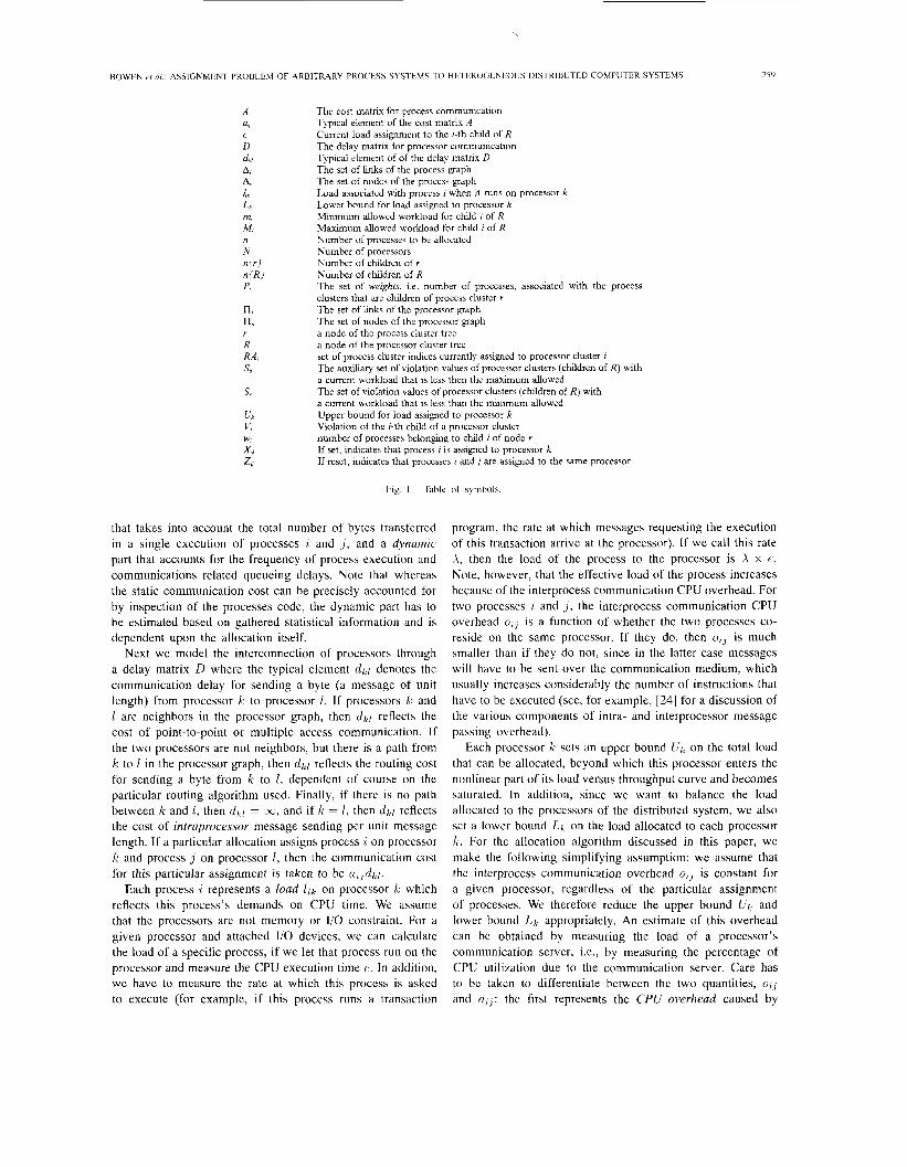
We conceive of a distributed system as composed of a set of nodes representing the active processing agents (e.g., host computer complexes in a computer network, individual processors in a multiprocessor system or a local area network, etc.) and an interconnection structure providing full connectivity between the nodes (e.g., communication lines in a long-haul computer network, shared memory modules or a bus in a multiprocessor system, a ring or a star topology in a local area network). The notation that we introduce throughout the paper is summarized in Fig. 1.

Given a set of processes A,, a set of processors rI, and their logical and physical interconnection structure, respectively, we define the process graph A = (An, Al), where A, is a set of links defined as: Al = { ( i : j ) 1 ( i , j ) denotes logical communication between processes i and j } . Similarly we define the processor graph I3 = (rI,,l&), where rIl = { ( k , l ) I (k, I) denotes a physical communication link between processors k and 1 ) .

The process allocation problem can be formulated as a quadratic assignment problem, and as such is similar to several other assignment problems such as facilities location, space allocation, scheduling and routing [ 171. These problems differ from the linear assignment problem in that the entities to be assigned are treated as a set of interconnected, rather than independent, objects (e.g., a facilities location problem in which the cost of materials flow between facilities is an important consideration). In our case, the interconnection of processes is modeled by a cost matrix A with a typical element aij , denoting the volume of communication between processes z and j . If the link ( i , j ) @Al then aij = 0. Also we take aii = 0, V i . The communication cost can be thought of as being composed of two parts: a static part

BOWEN cf a/ ' ASSIGNMENT PROBLEM OF ARBITRARY PROCESS S Y S l t M S TO HFI'EKOGENEOUS DISTRIBUTED COMPUTER SYSTEMS 259

The cost matrix for process communication Typical element of the cost matnx A Current load assignment to the i-th child of R The delay matrix for processor communication Typical element of of the delay matrix D The set of links of the process graph The set of nodes of the process graph Load associated with process i when it runs on processor k Lower bound for load assigned to processor k Minimum allowed workload for child i of R Maximum allowed workload for child i of R Number of processes to be allocated h'umber of processors Number of children of r Number of children of R The set of weights, i.e. number of processes, associated with the process clusters that are children of process cluster r The set of links of the processor graph The set of nodes of the processor graph a node of the process cluster tree a node of the processor cluster tree set of process cluster indices c u m " > - assigned to processor cluster i The auxiliary set of violation values of processor clusters (children of R ) with a current workload that is less then the maximum allowed The set of violation values of processor clusters (children of R ) with a current workload that is less than the minimum allowed Upper bound for load assigned to processor k Violation of the i-th child of a processor cluster number of processes belonging to child i of node r If set, indicates that process i is assigned to processor k If reset, indicates that processes i and j are assigned to the same processor

Fig. 1. Table of \ymhols

that takes into account the total number of bytes transferred in a single execution of processes i and j , and a dynamic part that accounts for the frequency of process execution and communications related queueing delays. Note that whereas the static communication cost can be precisely accounted for by inspection of the processes code, the dynamic part has to be estimated based on gathered statistical information and is dependent upon the allocation itself.

Next we model the interconnection of processors through a delay matrix D where the typical element d k r denotes the communication delay for sending a byte (a message of unit length) from processor k to processor 1. If processors k and II are neighbors in the processor graph, then (1k.l reflects the cost of point-to-point or multiple access communication. If the two processors are not neighbors, but there is a path from IC to 1 in the processor graph, then d k l reflects the routing cost for sending a byte from k to I , dependent of course on the particular routing algorithm used. Finally, if there is no path between k and I , then d ~ ; , = x, and if k = 1, then dI;[ reflects the cost of intraprocessor message sending per unit message length. If a particular allocation assigns process ,i on processor k and process j on processor I , then the communication cost for this particular assignment is taken to be ( L , J ~ I ; ~ .

Each process i represents a load l i k on processor k which reflects this process's demands on CPU time. We assume that the processors are not memory or I/O constraint. For a given processor and attached I/O devices, we can calculate the load of a specific process, if we let that process run on the processor and measure the CPU execution time p . In addition, we have to measure the rate at which this process is asked to execute (for example, if this process runs a transaction

program, the rate at which messages requesting the execution of this transaction arrive at the processor). If we call this rate A, then the load of the process to the processor is A x e . Note, however, that the effective load of the process increases because of the interprocess communication CPU overhead. For two processes i and j , the interprocess communication CPU overhead o,, is a function of whether the two processes co- reside on the same processor. If they do, then oLj is much smaller than if they do not, since in the latter case messages will have to be sent over the communication medium, which usually increases considerably the number of instructions that have to be executed (see, for example, [24] for a discussion of the various components of intra- and interprocessor message passing overhead).

Each processor k sets an upper bound 111; on the total load that can be allocated, beyond which this processor enters the nonlinear part of its load versus throughput curve and becomes saturated. In addition, since we want to balance the load allocated to the processors of the distributed system, we also set a lower bound Lk. on the load allocated to each processor k . For the allocation algorithm discussed in this paper, we make the following simplifying assumption: we assume that the interprocess communication overhead oil is constant for a given processor, regardless of the particular assignment of processes. We therefore reduce the upper bound UI; and lower bound LI; appropriately. An estimate of this overhead can be obtained by measuring the load of a processor's communication server, i.e., by measuring the percentage of CPU utilization due to the communication server. Care has to be taken to differentiate between the two quantities, o;j and U,]: the first represents the CPU overhead caused by

260 IEEE TRANSACTIONS ON COMPUTERS, VOL. 41, NO. 3, MARCH 1992

the communication of the two processes 7 and 3 . The latter denotes the communication delay, caused by the transmission of messages, contention in a multihop network, etc., incurred by the two communicating processes 1 and 3 .

In addition, note that by setting l , k = 00 for some of the k’s , we can model a process’s preference (affinity) in being assigned to specific processors only. Some researchers have proposed algorithms for allocating processes to processors under these preference constraints [lo]. Let X,k= 1 if process i is assigned to processor k and 0 otherwise. Then the processor capacity and load balancing constraints can be written as

n

L k 5 clikxik 5 u k V k . k = l ; . . , N (4.1) Z = l

where n is the total number of processes and N is the total number of processors.

In addition, since a process can be assigned to only one processor, we have the following constraint:

The minimization of the communication cost can now be written as

n n N N

~ j k l

A further simplifying assumption is that we treat all processes as equals in terms of the load that they represent to the processors. Typically, in large transaction processing centers there is a small number-probably no more than one hundred-f very active and resource demanding transaction types (processes) and a large number-probably in the thousands-f rarely, if ever, used transaction types. Only the allocation of the active transaction types has an impact on the performance of the center, not the allocation of the remaining thousands. We assume that these active processes represent roughly equal workloads, and we normalize their load to one. We call this assumption the “unit workload assumption.” Furthermore, we assume that d k k = 0 V k , k = 1; . . . , N , i.e., that intraprocessor message passing incurs a negligible communication cost as compared to the interprocessor one. We feel that this is a fully justified assumption for all existing distributed systems.

In the next two sections we describe our approach to process allocation. We propose the following combination of heuristic techniques: making use of a clustering algorithm, organize the graphs A and ll in hierarchies of clusters using the weights on their links as the clustering (similarity) measure. Call C and T the resulting process and processor cluster trees, respectively. In “Allocation Algorithm,” we show how to map the nodes of C to the nodes of T . This mapping defines an assignment of processes to processors. The basic idea of the clustering algorithm is to start with a weighted graph where each node represents a lowest-level cluster (a leaf in the associated cluster tree). We then form clusters of the next higher level by grouping pairs of nodes connected with links of maximum

weight. These pairs are then considered single nodes for the next iteration of the algorithm. Termination occurs when there is only one node left, the root of the cluster tree.

IV. CLUSTERING

Hagouel [ 111 presents a comprehensive survey of clustering algorithms. He distinguishes between two classes of clustering:

1) Agglomerative Algorithms-The graph is initially considered to have N clusters of 1 element each. N - 1 passes are made through the graph where each pass merges the two most similar clusters.

2) Divisive Algorithms-Initially, the graph is considered to be a single cluster, and then is successively split until the final clusters are of the desired size.

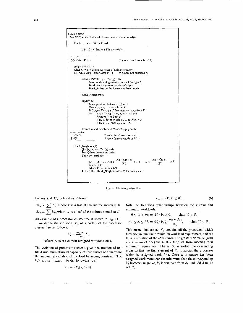
The algorithm presented is a variation of the agglomerative algorithm which uses the weight between nodes as the similarity criterion. Fig. 8 shows a formal definition of the algorithm. The input to this algorithm is a graph G = (V, F ) where V is a set of nodes and F is a set of edges. Associated with F is the set E , which contains the weights of all edges in F .

The first step is to copy the graph G into a working graph G’. Since an agglomerative algorithm is used, a series of intermediate passes are made which cluster the nodes with the greatest affinity. During each intermediate pass, each node must be put into a cluster. Note that a cluster can consist of a single node. This case would occur for a disjoint node (i.e., not communicating with any neighbors). Once an intermediate cluster has been made, all nodes but one are removed from the working graph (G’). This single node acts as a representative for the removed nodes during subsequent iterations of the algorithm. An intermediate pass terminates when all nodes have been clustered, and the algorithm terminates when V’ contains a single node.

An array is introduced to track when nodes have been clustered. Before an intermediate pass is begun, c(v,) is set to zero for all node in V’. As the intermediate pass clusters nodes, some c(v,) values are set to one while other nodes are entirely removed from V’. The intermediate pass terminates when all nodes in V’ have a .(vi) value equal to one.

The first step of the intermediate pass is to select a pivot node. This node is the one adjacent to the largest edge in the graph. Since there are at least two of these nodes, the following rules are also applied:

1) Break ties by greatest number of edges from node 2) Break ties by selecting lowest numbered node.

The next step is to select all the neighbors of the pivot node which have not yet been clustered. These are sorted into descending order based on the edge weight between the neighbor and the pivot. The set of all neighbors and the pivot node are now to be considered for clustering into a single node. The criteria used for selection of the pivot ensures that the subgraph now being considered for clustering in fact contains the largest edge in the graph.

The threshold value,. used to select candidates for inclusion into a cluster, is dependent upon the value of the weights e z J . This parameter allows the set of edges within a cluster to have approximately equal weights. This routine is recursively called

BOWEN c/ o/ . : ASSIGNMENT PROBLEM OF ARBITRARY PROCESS SYSTEMS TO HETEROGENEOUS DISTKIUUTED (’OMPUTEK S Y S l E M S 7 0 I

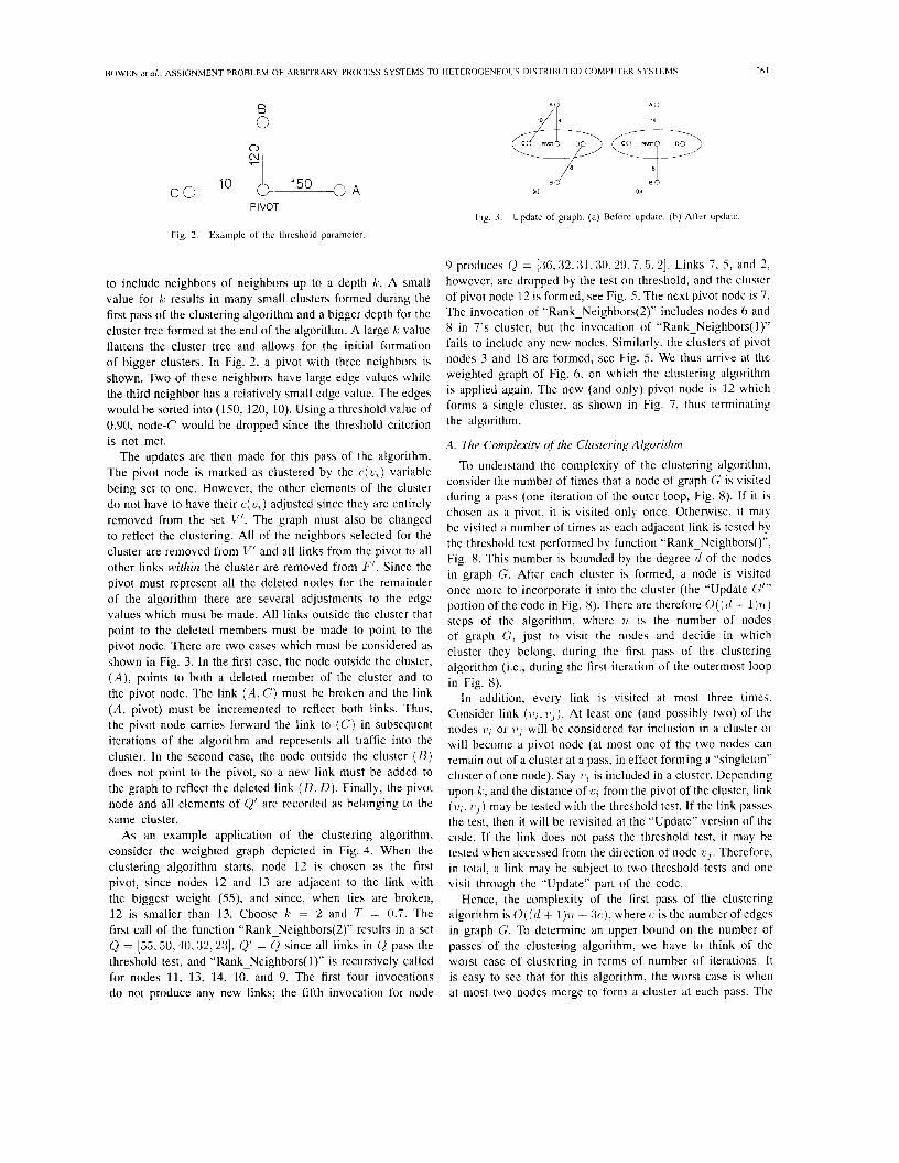
PIVOT Fig. 3. Update of graph. (a) Before update. (b) After update

Fig. 2. Example of the threshold parameter.

to include neighbors of neighbors up to a depth k . A small value for k results in many small clusters formed during the first pass of the clustering algorithm and a bigger depth for the cluster tree formed at the end of the algorithm. A large k value flattens the cluster tree and allows for the initial formation of bigger clusters. In Fig. 2, a pivot with three neighbors is shown. Two of these neighbors have large edge values while the third neighbor has a relatively small edge value. The edges would be sorted into (150, 120, 10). Using a threshold value of 0.90, node-C would be dropped since the threshold criterion is not met.

The updates are then made for this pass of the algorithm. The pivot node is marked as clustered by the c ( u t ) variable being set to one. However, the other elements of the cluster do not have to have their c(%iz) adjusted since they are entirely removed from the set V’. The graph must also be changed to reflect the clustering. All of the neighbors selected for the cluster are removed from V’ and all links from the pivot to all other links within the cluster are removed from F’. Since the pivot must represent all the deleted nodes for the remainder of the algorithm there are several adjustments to the edge values which must be made. All links outside the cluster that point to the deleted members must be made to point to the pivot node. There are two cases which must be considered as shown in Fig. 3. In the first case, the node outside the cluster, (A), points to both a deleted member of the cluster and to the pivot node. The link (-4. C) must be broken and the link (A, pivot) must be incremented to reflect both links. Thus, the pivot node carries forward the link to (C) in subsequent iterations of the algorithm and represents all traffic into the cluster. In the second case, the node outside the cluster (B) does not point to the pivot, so a new link must be added to the graph to reflect the deleted link ( B . D ) . Finally, the pivot node and all elements of C)‘ are recorded as belonging to the same cluster.

As an example application of the clustering algorithm, consider the weighted graph depicted in Fig. 4. When the clustering algorithm starts, node 12 is chosen as the first pivot, since nodes 12 and 13 are adjacent to the link with the biggest weight (SS), and since, when ties are broken, 12 is smaller than 13. Choose k = 2 and T = 0.7. The first call of the function “Rank-Neighbors(2)” results in a set Q = [%.SO. 40.32,23]. Q‘ = (2 since all links in Q pass the threshold test, and “Rank-Neighbors( 1)” is recursively called for nodes 11, 13, 14, 10, and 9. The first four invocations do not produce any new links; the fifth invocation for node

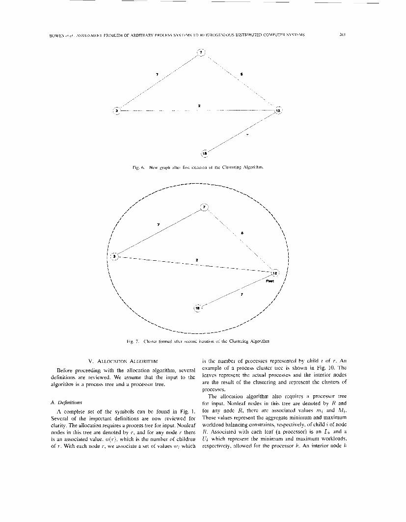
9 produces Q = [36,32.31.30,29.7.5.2]. Links 7, 5, and 2, however, are dropped by the test on threshold, and the cluster of pivot node 12 is formed, see Fig. 5. The next pivot node is 7. The invocation of “Rank-Neighbors(2)” includes nodes 6 and 8 in 7’s cluster, but the invocation of “Rank-Neighbors(1)” fails to include any new nodes. Similarly, the clusters of pivot nodes 3 and 18 are formed, see Fig. 5. We thus arrive at the weighted graph of Fig. 6, on which the clustering algorithm is applied again. The new (and only) pivot node is 12 which forms a single cluster, as shown in Fig. 7, thus terminating the algorithm.

A. The Complexity of the Clustering Algorithm

To understand the complexity of the clustering algorithm, consider the number of times that a node of graph G is visited during a pass (one iteration of the outer loop, Fig. 8). If i t is chosen as a pivot, i t is visited only once. Otherwise, i t may be visited a number of times as each adjacent link is tested by the threshold test performed by function “Rank-Neighborso”, Fig. 8. This number is bounded by the degree d of the nodes in graph G. After each cluster is formed, a node is visited once more to incorporate it into the cluster (the “Update G’” portion of the code in Fig. 8). There are therefore O ( ( d + I )??) steps of the algorithm, where ri is the number of nodes of graph C:, just to visit the nodes and decide in which cluster they belong, during the first pass of the clustering algorithm (i.e., during the first iteration of the outermost loop in Fig. 8).

In addition, every link is visited at most three times. Consider link ( u ; . v J ) . At least one (and possibly two) of the nodes 1 1 ; or ‘U, will be considered for inclusion in a cluster or will become a pivot node (at most one of the two nodes can remain out of a cluster at a pass, in effect forming a “singleton” cluster of one node). Say 71, is included in a cluster. Depending upon k , and the distance of 7 ~ , from the pivot of the cluster, link ( v , . ‘ L i J ) may be tested with the threshold test. If the link passes the test, then i t will be revisited at the “Update” version of the code. If the link does not pass the threshold test, it may be tested when accessed from the direction of node vj . Therefore, in total, a link may be subject to two threshold tests and one visit through the “Update” part of the code.

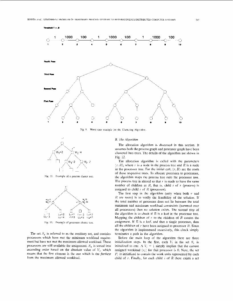
Hence, the complexity of the first pass of the clustering algorithm is O ( ( d + 1)rr + 3 c ) , where (: is the number of edges in graph G. To determine an upper bound on the number of passes of the clustering algorithm, we have to think of the worst case of clustering in terms of number of iterations. I t is easy to see that for this algorithm, the worst case is when at most two nodes merge to form a cluster at each pass. The


Fig. 4. Example weighted graph for the Clustering Algorithm.

n). For small to O(n1ogn).

BOWEN ef al.: ASSIGNMENT PROBLEM OF ARBITRARY PROCESS SYSTEMS 10 HEI'EROGENEOUS UISTRIBUlED COMPUTER SYSTEMS 263

Fig. 6. New graph after first iteration of the Clustering Algorithm

----_____------- Fig. 7. Cluster formed after second iteration of the Clustering Algorithm.

V. ALLOCATION ALGORITHM

Before proceeding with the allocation algorithm, several definitions are reviewed. We assume that the input to the algorithm is a process tree and a processor tree.

A. Definitions

A complete set of the symbols can be found in Fig. 1. Several of the important definitions are now reviewed for clarity. The allocation requires a process tree for input. Nonleaf nodes in this tree are denoted by r , and for any node r there is an associated value, n ( r ) , which is the number of children of T . With each node r , we associate a set of values w, which

is the number of processes represented by child i of r. An example of a process cluster tree is shown in Fig. 10. The leaves represent the actual processes and the interior nodes are the result of the clustering and represent the clusters of processes.

The allocation algorithm also requires a processor tree for input. Nonleaf nodes in this tree are denoted by R and for any node R, there are associated values r n i and Mi. These values represent the aggregate minimum and maximum workload balancing constraints, respectively, of child 1; of node R. Associated with each leaf (a processor) is an LI, and a l!k which represent the minimum and maximum workloads, respectively, allowed for the processor I C . An interior node k


iiven a graph G = (V,F) where V is a set of nodes and F is a set of edges.

V = {v,, ... , vn}, F s V x V and:

If (v!, v,) E F then e, E is the weight

G' = G D O w h i l e I V ' I > l / * more than 1 node in V' */

c(v') = 0 v v' E V' Clear C / * C will hold all nodes of a single cluster': DO while c(v') = 0 for some v' E V' / * Nodes not clustered * i

Select a PIVOT (v, E V'AC(V,) = 0). Select node with greatest e,, 3 v, E V'AC(V,) = 0 Break ties by greatest number of edges Break further ties by lowest numbered node

Rank-Neighbors(k)

Update G': Mark pivot as clustered (c(v,) = 1) Vv, E C, v, # v, remove v, from V' If (v,, v,) E F AV,, v, E C then remove (v,, v,) from F VV,, Y, 3 V, E C A V,dc A (Vn,V,) E F A V , # V,

Remove (v,,v,) from F If (v,, v,)dF then add (v,, v,) to F ; e , = e, If (v,, v,) E F then e,, = e,, + e,

Record v, and members of C as belonging to the same cluster

END END

I' nodes in V' not clustered */ /' more than one node in V' */

Rank-Neighbors(k) Q = {e,, 1 v,, v, E Ffic(v,) = 0) Sort Q into descending order Drop on threshold:

where V, = Lu I e,, E Q'] If k > 1 then Rank-Neighbors ( k - 1) for each v, E C

Fig. 8. Clustering Algorithm

has mk and Mk defined as follows:

mk =

Mk =

Lk, where k is a leaf of the subtree rooted at R

U,, where k is a leaf of the subtree rooted at R.

An example of a processor cluster tree is shown in Fig. 11.

cluster tree as follows: We define the violation, V,, of a node a of the processor

ma - c, m,

V, = -,

where c, is the current assigned workload on i.

The violation of processor cluster i gives the fraction of un- filled minimum allowed capacity of that cluster and therefore the amount of violation of the load balancing constraint. The V,'s are partitioned into the following sets:

s, = {qV, > 0)

sf3 = {KlV, IO}. (6)

Note the following relationships between the current and minimum workloads:

0 5 c, < m, + 1 2 V, > 0, thus V , E S,

, thus V, E Sa. m, - M, m, 5 c, I M, + 0 2 V, 2 - m,

This means that the set S, contains all the processors which have not yet met their minimum workload requirement, and are thus in violation of the constraints. The greater this value (with a maximum of one) the further they are from meeting their minimum requirement. The set S, is sorted into descending order so that the first element of S, is always the processor which is assigned work first. Once a processor has been assigned work more than the minimum, then the corresponding V, becomes negative, V , is removed from S, and added to the set Sa.

BOWFN er a / ASSIGNMENT PROBLEM OF ARBITRARY PROCESS SYSTEMS TO HETEROGENEOUS DISTRIBUTED COMPUTER SYSTEMS

1 1000 100 1 1000 100 1 1000 100 L/ W v v LJ v U U

1 2 3 4 s 6 7 8 # 1D

1 a 3 4 E 7 8 10

Fig. 9. Worst case example for the Clustering Algorithm

r ' n

B. The Algorithm

Fig. 10. Example of a process cluster tree

R ' n

265

The allocation algorithm is discussed in this section. It assumes both the process graph and processor graph have been clustered into trees. The details of the algorithm are shown in Fig. 12.

The allocation algorithm is called with the parameters ( T > R) , where T is a node in the process tree and R is a node in the processor tree. For the initial call, ( T , R) are the roots of these respective trees. To allocate processes to processors, the algorithm maps the process tree onto the processor tree. The process tree is altered so that T is made to have the same number of children as R, that is, child i of T (process) is assigned to child i of R (processor).

The first step in the algorithm (only when both T and R are roots) is to verify the feasibility of the solution. If the total number of processes does not lie between the total minimum and maximum workload constraints (summed over all processors) then no solution exists. The second step of the algorithm is to check if R is a leaf in the processor tree. Mapping the children of T to the children of R creates the assignment. If R is a leaf, and thus a single processor, then all the children of T have been assigned to processor R. Since the algorithm is implemented recursively, this check simply terminates a path in the algorithm.

Before the main loop of the algorithm there are three initialization steps. In the first, each V , in the set S,, is initialized to one. A V, = 1 simply implies that the current assigned workload ( c i ) for that processor is 0. Next, the set P,. is initialized to contain the work units represented by each child of T . Finally, for each child 'i of R there exists a set

The set Sa is referred to as the auxiliary set, and contains processors which have met the minimum workload requirement but have not met the maximum allowed workload. These processors are still available for assignment. Sa is sorted into ascending order based on the absolute value of V,, which means that the first element is the one which is the furthest from the maximum allowed workload.

L1'1 L ~ = Z ~ , = l L z = 3 L 3 = 2 u,=3 uz=4 u1=3 uz=5 U,-2

Fig. 11. Example of processor cluster tree.

IEEE TRANSACTIONS ON COMPUTERS, VOL. 41, NO. 3, MARCH 1992 266

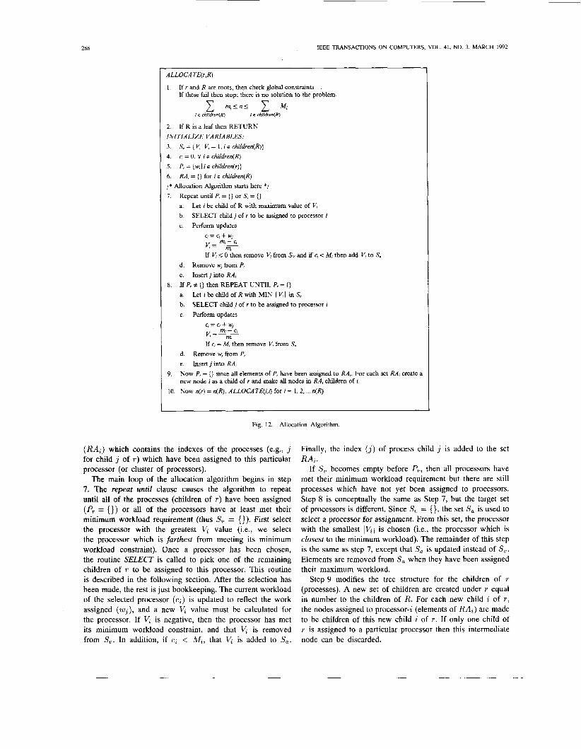
ALLOCA TE(r,R)

1. If r and R are roots, then check global constraints If these fail then stop; there is no solution to the problem

.

m i < n < Mi i E children(R) i E children(R)

2. INITIALIZE VARIABLES: 3 . 4. 5. 6. / * Allocation Algorithm starts here */ 7.

If R is a leaf then RETURN

S, = (V , I V, = 1, i E chi/dren(R)} c, = 0, V i E children(R) f, = {w8 I i E children(r)} RA, = {} for i E children(R)

Repeat until f, = {} or S. = {} a. b. c. Perform updates

Let i be child of R with maximum value of V, SELECT child j of r to be assigned to processor i

c, = c, + w,

If V, < 0 then remove V, from Sv and if c, <: M, then add V, to Sa

m! - c, K = m ,

d. Remove w, from f, e . Insert j into RA, Jf f, # (} then REPEAT UNTIL f, = () a.

b. c. Perfom updates

8.

Let i be child of R with MIN 1 V,I in So SELECT child j of r to be assigned to processor i

If c, = M, then remove V, from S,

d. Remove w, from f, e . Insert j into RA,

9. Now f, = {} since all elements o f f , have been assigned to RA,. For each set RA, create a new node i as a child of r and make all nodes in RA, children of i.

IO. Now n(r) = n(R). ALLOCATE(i,z) for i = 1,2, ... n(R)

Fig. 12. Allocation Algorithm.

(RA,) which contains the indexes of the processes (e.g., j for child j of T ) which have been assigned to this particular processor (or cluster of processors).

The main loop of the allocation algorithm begins in step 7. The repeut until clause causes the algorithm to repeat until all of the processes (children of r ) have been assigned (Pr = {}) or all of the processors have at least met their minimum workload requirement (thus S, = {}). First select the processor with the greatest V, value (i.e., we select the processor which is furthest from meeting its minimum workload constraint). Once a processor has been chosen, the routine SELECT is called to pick one of the remaining children of r to be assigned to this processor. This routine is described in the following section. After the selection has been made, the rest is just bookkeeping. The current workload of the selected processor (c,) is updated to reflect the work assigned (wJ), and a new V , value must be calculated for the processor. If V, is negative, then the processor has met its minimum workload constraint, and that V, is removed from S,. In addition, if c, < Mz, that V , is added to Sa.

Finally, the index ( j ) of process child j is added to the set RA,.

If S, becomes empty before Pr, then all processors have met their minimum workload requirement but there are still processes which have not yet been assigned to processors. Step 8 is conceptually the same as Step 7, but the target set of processors is different. Since S, = {}, the set Sa is used to select a processor for assignment. From this set, the processor with the smallest IV,l is chosen (i.e., the processor which is closest to the minimum workload). The remainder of this step is the same as step 7, except that Sa is updated instead of S,. Elements are removed from Sa when they have been assigned their maximum workload.

Step 9 modifies the tree structure for the children of r (processes). A new set of children are created under r equal in number to the children of R. For each new child i of r , the nodes assigned to processor-i (elements of RAi) are made to be children of this new child i of r. If only one child of r is assigned to a particular processor then this intermediate node can be discarded.

B O W t N er ul ASSIGNMENT PROBLEM OF ARBITRARY PROCESS SYSTEMS TO HETEROGENEOUS UlSTRlBU TbD COMPUTER SYSTEMS 261

The final step is to recursively call the algorithm. At this point, the children of r' have been assigned to children of R so that both sr and R have the same number of children. For each of these assignments, a call to ALLOCATE(i. i ) is made for each of the pairs of children.

The unit workload assumption and the check for the minimum workload constraint during the SELECT process guar- antee that the algorithm terminates with a solution. If the unit workload assumption were to be dropped, then modifications would have to be made to ensure that the workload constraints are satisfied.

The SELECTion Routine: This routine selects child j of r'

(cluster of processes) with the maximum 7ii,, to be assigned to processor i . SELECT checks whether there is still enough work in P,. to meet the minimum workload requirement of all processor nodes that are children of R after the removal of j from E',..

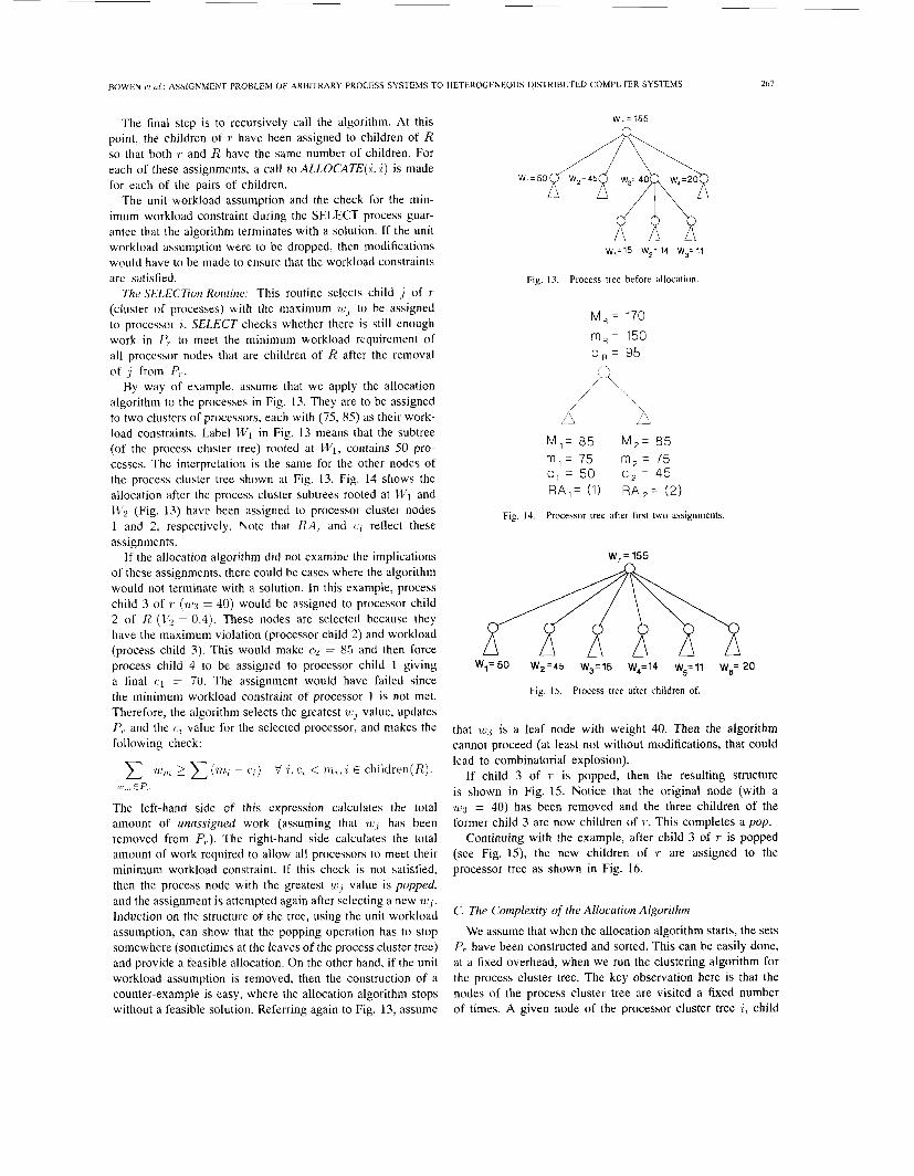
By way of example, assume that we apply the allocation algorithm to the processes in Fig. 13. They are to be assigned to two clusters of processors, each with (75, 85) as their workload constraints. Label W1 in Fig. 13 means that the subtree (of the process cluster tree) rooted at IVl, contains 50 processes. The interpretation is the same for the other nodes of the process cluster tree shown at Fig. 13. Fig. 14 shows the allocation after the process cluster subtrees rooted at W1 and W, (Fig. 13) have been assigned to processor cluster nodes 1 and 2, respectively. Note that RA, and I : L reflect these assignments.

If the allocation algorithm did not examine the implications of these assignments, there could be cases where the algorithm would not terminate with a solution. In this example, process child 3 of 1' ( w g = 40) would be assigned to processor child 2 of R (V2 = 0.4). These nodes are selected because they have the maximum violation (processor child 2) and workload (process child 3). This would make c2 = 85 and then force process child 4 to be assigned to processor child 1 giving a final c1 = 70. The assignment would have failed since the minimum workload constraint of processor 1 is not met. Therefore, the algorithm selects the greatest w j value, updates P,. and the c, value for the selected processor, and makes the following check:

1 'w,,l 2 (m, - c,) v i . c, < mt , i E ckiildren(R). IC ,> , EP,

The left-hand side of this expression calculates the total amount of unassigned work (assuming that ,wJ has been removed from P,.). The right-hand side calculates the total amount of work required to allow all processors to meet their minimum workload constraint. If this check is not satisfied, then the process node with the greatest w j value is popped, and the assignment is attempted again after selecting a new w3. Induction on the structure of the tree, using the unit workload assumption, can show that the popping operation has to stop somewhere (sometimes at the leaves of the process cluster tree) and provide a feasible allocation. On the other hand, if the unit workload assumption is removed, then the construction of a counter-example is easy, where the allocation algorithm stops without a feasible solution. Referring again to Fig. 13, assume

W,=155 -

w,=15 W,=14 W,= 11

Fig. 13. Process tree before allocation

M,= 170 m R = 150 c , = 95

A /..;\ " 1 (2

M,= 85 M,= 85 m , = 75 m , = 7 5 c , = 50 c , = 4 5 RA,= (1) RA,= (2)

Fig. 14. Processor tree after first two assignments.

W, = 155 n

W,=50 W,=45 W,=15 W,=14 W,=11 W,=20

Fig. 15. Process tree after children of.

that w3 is a leaf node with weight 40. Then the algorithm cannot proceed (at least not without modifications, that could lead to combinatorial explosion).

If child 3 of r is popped, then the resulting structure is shown in Fig. 15. Notice that the original node (with a 7 1 ~ = 40) has been removed and the three children of the former child 3 are now children of T . This completes a pop.

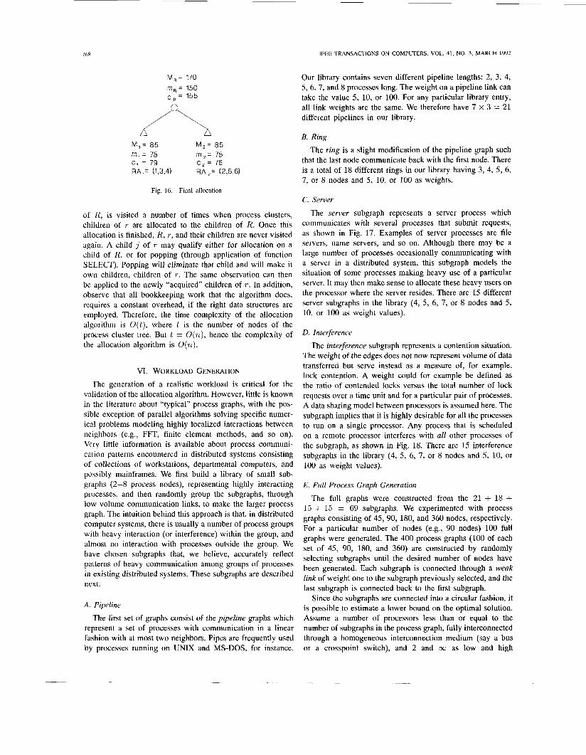
Continuing with the example, after child 3 of r is popped (see Fig. 15), the new children of 7' are assigned to the processor tree as shown in Fig. 16.

C. The Complexity of the Allocation Algorithm

We assume that when the allocation algorithm starts, the sets P,. have been constructed and sorted. This can be easily done, at a fixed overhead, when we run the clustering algorithm for the process cluster tree. The key observation here is that the nodes of the process cluster tree are visited a fixed number of times. A given node of the processor cluster tree i , child

IEEE TRANSACTIONS ON COMPUTERS, VOL. 41, NO. 3, MARCH 1992

M,= 170 m R = 150 c = 155 n

M,= 85 M 2 = 85 m , = 75 m z = 75 c , = 79 c,= 76 RA,= (1,3,4) RA,= (2,5,6)

Fig. 16. Final allocation.

of R, is visited a number of times when process clusters, children of T are allocated to the children of R. Once this allocation is finished, R, r , and their children are never visited again. A child j of T may qualify either for allocation on a child of R, or for popping (through application of function SELECT). Popping will eliminate that child and will make it own children, children of T . The same observation can then be applied to the newly “acquired children of r . In addition, observe that all bookkeeping work that the algorithm does, requires a constant overhead, if the right data structures are employed. Therefore, the time complexity of the allocation algorithm is O(t ) , where t is the number of nodes of the process cluster tree. But t = O(n) , hence the complexity of the allocation algorithm is O(n) .

VI. WORKLOAD GENERATION

The generation of a realistic workload is critical for the validation of the allocation algorithm. However, little is known in :he literature about “typical” process graphs, with the possible exception of parallel algorithms solving specific numerical problems modeling highly localized interactions between neighbors (e.g., FFT, finite element methods, and so on). Very little information is available about process communication patterns encountered in distributed systems consisting of collections of workstations, departmental computers, and possibly mainframes. We first build a library of small subgraphs (2-8 process nodes), representing highly interacting processes, and then randomly group the subgraphs, through low volume communication links, to make the larger process graph. The intuition behind this approach is that, in distributed computer systems, there is usually a number of process groups with heavy interaction (or interference) within the group, and almost no interaction with processes outside the group. We have chosen subgraphs that, we believe, accurately reflect patterns of heavy communication among groups of processes in existing distributed systems. These subgraphs are described next.

A. Pipeline

The first set of graphs consist of the pipeline graphs which represent a set of processes with communication in a linear fashion with at most two neighbors. Pipes are frequently used by processes running on UNIX and MS-DOS, for instance.

Our library contains seven different pipeline lengths: 2, 3, 4, 5, 6, 7, and 8 processes long. The weight on a pipeline link can take the value 5 , 10, or 100. For any particular library entry, all link weights are the same. We therefore have 7 x 3 = 21 different pipelines in our library.

B. Ring

The ring is a slight modification of the pipeline graph such that the last node communicate back with the first node. There is a total of 18 different rings in our library having 3, 4, 5, 6, 7, or 8 nodes and 5, 10, or 100 as weights.

C. Server

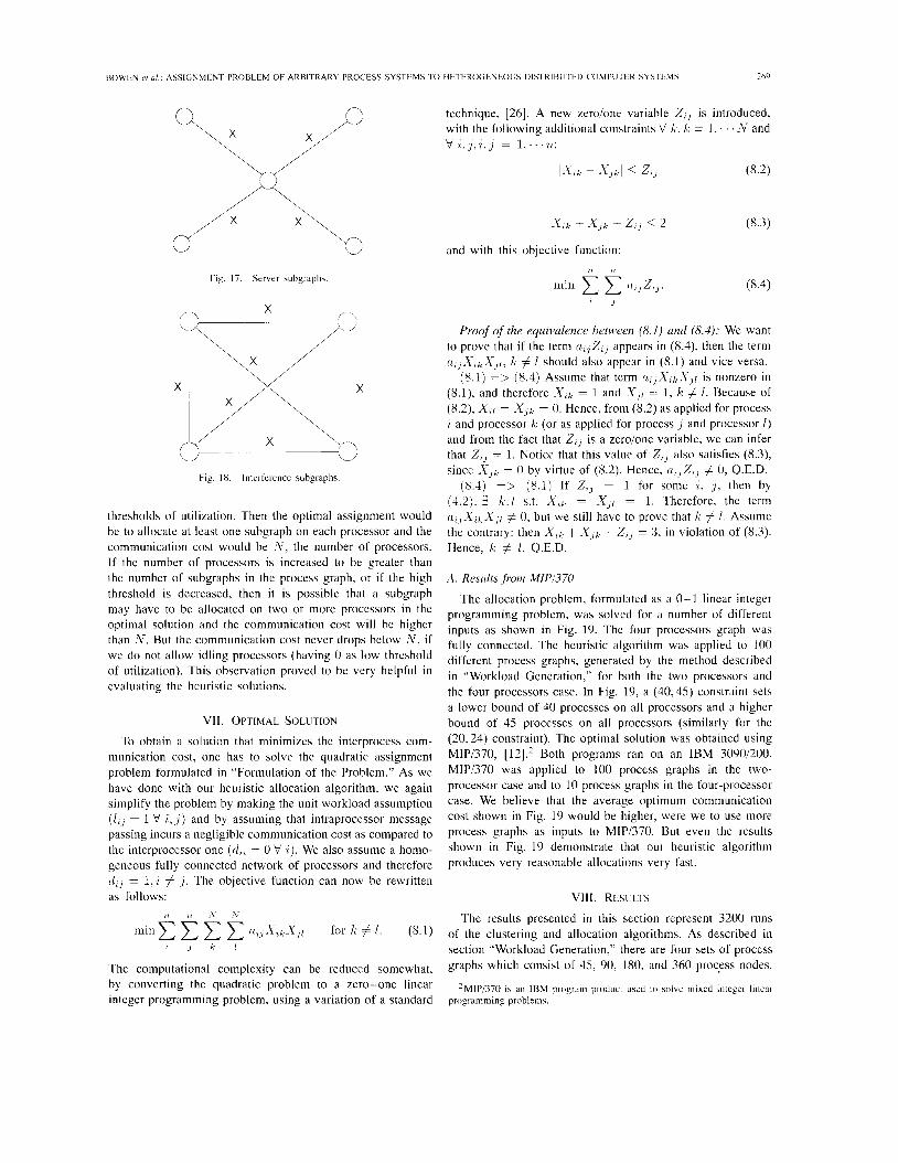
The server subgraph represents a server process which communicates with several processes that submit requests, as shown in Fig. 17. Examples of server processes are file servers, name servers, and so on. Although there may be a large number of processes occasionally communicating with a server in a distributed system, this subgraph models the situation of some processes making heavy use of a particular server. It may then make sense to allocate these heavy users on the processor where the server resides. There are 15 different server subgraphs in the library (4, 5, 6, 7, or 8 nodes and 5 , 10, or 100 as weight values).

D. Interference

The interference subgraph represents a contention situation. The weight of the edges does not now represent volume of data transferred but serve instead as a measure of, for example, lock contention. A weight could for example be defined as the ratio of contended locks versus the total number of lock requests over a time unit and for a particular pair of processes. A data sharing model between processors is assumed here. The subgraph implies that it is highly desirable for all the processes to run on a single processor. Any process that is scheduled on a remote processor interferes with all other processes of the subgraph, as shown in Fig. 18. There are 15 interference subgraphs in the library (4, 5 , 6, 7, or 8 nodes and 5, 10, or 100 as weight values).

E. Full Process Graph Generation

The full graphs were constructed from the 21 + 18 + 15 + 15 = 69 subgraphs. We experimented with process graphs consisting of 45, 90, 180, and 360 nodes, respectively. For a particular number of nodes (e.g., 90 nodes) 100 full graphs were generated. The 400 process graphs (100 of each set of 45, 90, 180, and 360) are constructed by randomly selecting subgraphs until the desired number of nodes have been generated. Each subgraph is connected through a weak link of weight one to the subgraph previously selected, and the last subgraph is connected back to the first subgraph.

Since the subgraphs are connected into a circular fashion, it is possible to estimate a lower bound on the optimal solution. Assume a number of processors less than or equal to the number of subgraphs in the process graph, fully interconnected through a homogeneous interconnection medium (say a bus or a crosspoint switch), and 2 and cc as low and high

BOWEN er U / . : ASSIGNMENT PROBLEM OF ARBITRARY PROCESS S Y S T t M S ‘IO Hkl’EROGENEOUS DISTRIBUTED COMI’U’I-ER SYSl I:MS 269

“....;-i... technique, [26]. A new zero/one variable Z, , is introduced, with the following additional constraints V X . X: = 1. . . . AV and V / . , J . / . , J = 1 : . . / I :

(8.2)

Fig. 17. Server subgraphs

Fig. 18. Interference subgraphs.

thresholds of utilization. Then the optimal assignment would be to allocate at least one subgraph on each processor and the communication cost would be N , the number of processors. If the number of processors is increased to be greater than the number of subgraphs in the process graph, or if the high threshold is decreased, then it is possible that a subgraph may have to be allocated on two or more processors in the optimal solution and the communication cost will be higher than N . But the communication cost never drops below N , if we do not allow idling processors (having 0 as low threshold of utilization). This observation proved to be very helpful in evaluating the heuristic solutions.

VII. OPTIMAL SOLIJTION

To obtain a solution that minimizes the interprocess communication cost, one has to solve the quadratic assignment problem formulated in “Formulation of the Problem.” As we have done with our heuristic allocation algorithm, we again simplify the problem by making the unit workload assumption

= 1 b’ 6 , j ) and by assuming that intraprocessor message passing incurs a negligible communication cost as compared to the interprocessor one ( d , ~ = 0 b’ i ) . We also assume a homogeneous fully connected network of processors and therefore d i , = 1.% # j . The objective function can now be rewritten as follows:

/ , A /

The computational complexity can be reduced somewhat, by converting the quadratic problem to a zero-one linear integer programming problem, using a variation of a standard

and with this objective function: ? l , l

Proof of the equivalence between (8.1) und (8.4): We want to prove that if the term O , ~ Z ~ , appears in (8.4), then the term U~,A-~LX,/, h # / should also appear in (8.1) and vice versa.

(8.1) => (8.4) Assume that term u f J X z k X I / is nonzero in (8.1), and therefore = 1 and S,/ = 1, b # I . Because of (8.2), X,l = Xlk = 0. Hence, from (8.2) as applied for process I and processor k (or as applied for proce5s J and processor 1) and from the fact that Z,, is a zero/one variable, we can infer that Z,, = 1. Notice that this value of Z,, also satisfies (8.3), since L Y J ~ = 0 by virtuc of (8.2). Hence, u l l Z z J # 0, Q.E.D.

(8.4) => (8.1) If Z, , = 1 for Some /, J , then by (4.2) . 3 h.1 s.t. X , k = LY,l = 1. Therefore, the term u/ , -Y/kX,l # 0, but we still have to prove that k # 1. Assume the contrary: then X,k + X,k + Z, , = 3, in violation of (8.3). Hence, k # 1, Q.E.D.

A. Results from MIPI370

The allocation problem, formulated as a 0-1 linear integer programming problem, was solved for a number of different inputs as shown in Fig. 19. The four processors graph was fully connected. The heuristic algorithm was applied to 100 different process graphs, generated by the method described in “Workload Generation,” for both the two processors and the four processors case. In Fig. 19, a (40,45) constraint sets a lower bound of 40 processes on all processors and a higher bound of 45 processes on all processors (similarly for the (20,24) constraint). The optimal solution was obtained using MIPi370, [12].2 Both programs ran on an IBM 30901200. MIPi370 was applied to 100 process graphs in the two- processor case and to 10 process graphs in the four-processor case. We believe that the average optimum communication cost shown in Fig. 19 would be higher, were we to use more process graphs as inputs to MIPi370. But even the results shown in Fig. 19 demonstrate that our heuristic algorithm produces very reasonable allocations very fast.

VIII. RESULTS

The results presented in this section represent 3200 runs of the clustering and allocation algorithms. As described in section “Workload Generation,” there are four sets of process graphs which consist of 45, 90, 180, and 360 process nodes.

‘MIPi370 is an IBM program product used to solve mixcd integcr linear programming problems.

270

30-

n -

m -

y1 U

E l 5 - r%


Heur i s t i c Time

Optimal Time

H e u r i s t i c cost

Optimal cost

Worst-case A l l o c a t i o n cost

2 processors 4 processors 90 processes 90 processes ( 4 0 , 4 5 ) Cons t r a i nts ( 2 0 , 2 4 ) Cons t r a i n t s

0.581 sec Q.592 sec

4 .52 sec 1777.22 sec

39 .26

2 . 0 0 4 .20

4820

Fig. 19. Heuristic and optimal allocation, CPU time and communication cost.

Each set contains 100 graphs (i.e., there are a total of 400 process graphs). Four fully connected processor graphs with all weights equal to one were used in the experiment (2, 4, 8, and 16 processors).

For each matching of a set of process graphs to an individual processor graph, the clustering and allocation algorithms were executed with four different workload balancing constraints. We define the target workload to be that of a uniform workload distribution, thus

number of processes number of processors ’

target =

We further define a set of variances (lo%, 25%, 50%, and 98%) to calculate the minimum and maximum workload bounds.

L = target - target x variance U = target + target x variance.

The CPU consumption is a critical measure of this algorithm. In Fig. 20 we have graphed the CPU seconds, on an IBM 3090-200, required for the clustering and allocation algorithm for a variety of process nodes. The aim of the configurations used in this example was to show the growth in CPU consumption as the size of the system grows. For this reason we have decided to use processor configurations which always get approximately 22 process nodes per processor (i.e., 90 processes on 4 processors, 360 processes on 16 processors).

The results show that the algorithms are practical even for large configurations.

Again looking at a processor configuration which always get approximately 22 process nodes per processor (i.e., 90 processes on 4 processors, 360 processes on 16 processors), we have also studied the communication cost. Since the optimal solution is extremely time consuming to calculate, we have used a feature inherent to the process graphs to compare our solutions. The workload graphs were generated by connecting a collection of small (2-8 process nodes) nodes together to form a large process graph. These small graphs were connected by a “weak-link” of value one. One can intuitively imagine the optimal solution to assign these small subgraphs to a single processor. Then the only interprocessor communication is due to these “weak-links.” Therefore, we can state that a lower bound for the optimal solution is the number of processors in

CPU T i m e v s . P r o c e s s n o d e s 2 2 n o d e s p e r p r o c e s s o r

X of Process nodes

Fig. 20. CPU analysis.

Communication Cost 12 processes per processor

30 -I n 2 k B 16

Number of Processors

Fig. 21. Communication cost for 22 processes per processor.

the configuration. Fig. 21 shows the heuristic solutions for the same points that were shown in Fig. 20. The x axis shows the number of processors. 22 processes are being assigned to each processor. Therefore, the number of input nodes is changing for each processor configuration (i.e., 45 processes on 2 processors, 360 processes on 16 processors).

These numbers are the average of 100 runs on each given processor configuration. In each of the 100 runs a different process graph is being used for input. These results are extremely promising since they are very close to the lower bound of the optimal solution.

In addition to looking at a fixed number of processes/ processors, we also present results for taking the same set of processes and assigning them to a varying number of processors. In Fig. 22, 90 processes are assigned to 2, 4, 8, and 16 processors. The workload bounds used for these points were 50%. Note that the assigned number of processes per processor ‘gets smaller as the number of processors increase. These results again show that the algorithms are making very good assignments.

BOWEN e r U/: ASSIGNMENT PROBLEM OF ARBITRARY PROCESS SYSTEMS TO HETEROGENbOUS DISTRIBUTtD COMPUTER SYSTEMS

im

100

80

c 860

.- " U )

z E20

U

c 0 c U

c

.-

U

[

Communication Cost 90 Processes 50% Workload Variance

10780

7.05 150 -

I I I I 1 4 B 16

Number of processors

I

Fig. 22. Communication cost for 90 processes assigned to 2, 4, X, and 16 processors

80

.- .- :ji = a c

Z m E U 10

0

Cost at various workload bounds 8 processors - 180 processes

19.90 21.60 I

1 (mi41 (1617) (tl,JJ)

Load Balancing Constraints (LU) Fig. 23. Sen\itivity to workload bounds

As stated in the introduction of this section, the workload bounds were varied to determine the sensitivity of the algorithms to these parameters. The CPU time was not at all sensitive to the workload bounds but we found the solutions themselves to be rather sensitive.

Fig. 23 shows communication costs for the case where 180 processes are assigned to 8 processor nodes. The workload bounds were calculated using variances of 10, 25, 50, and 98%. The results are not immediately intuitive.

Using a variance of 10% the workload bounds are very tight (22-24 processes per processor). This case produces the worst results because the allocation algorithm is forced to split apart most of the subgraphs in the workload process graph. Variances of 25 and 50% produce good results because the allocation is able to maintain the affinity of the subgraphs.

One would think that using a variance of 98% would produce results better than using 25 and 50. This is not the case. As shown in the graph, this case produces worse results. Consider the following example. Assume that the process tree

Communication Cost 90 processes and 16 processors

(1.11) (U) Load Balancing Constraints (LU)

Fig. 24. Effects of tight workload bounds

27 1

L root had four subtrees each representing 44 units of work. Also assume that the processor tree root contains eight subtrees each with workload bounds of (1,44). The allocation algorithm would assign the first three subtrees from the process graph to the first three subtrees of the processor graph. This would leave one process subtree of 44 nodes to be assigned to five processor graphs. The single process subtree would now have to be "popped" several times to meet this allocation. Having tighter bounds, primarily the upper bound, produces more popping at the higher levels of the processor tree. The clustering has produced a tree with heavily communicating nodes at the bottom of the tree, therefore, popping at the top of the tree does not create a severe communication cost penalty. Once the popping is forced to go deep to the bottom of a process tree, the communication penalties become high.

The workload generations for these experiments produce a series of subgraphs (2-8 nodes) which are connected by a "weak-link" of weight one. It is interesting to measure the communication cost when the workload bounds are made so tight that these subgraphs must be split onto separate processors. In Fig. 24 the 90 node process graphs are assigned to 16 processors with all four workload variances. The target assignment for each processor is 5.6 processes per processor.

In the first two cases (98% and 50% variance) the communication costs are very reasonable. This is because the subgraphs are still able to be mostly assigned to one processor. Once the maximum workload bound goes below the subgraph size the solutions get dramatically worse. It should be noted, however, that even in the worst case (bounds of 5 , 6) the communication cost of 1945 is still reasonable. The total amount of communication for these processes nodes is 4569. Although we could not calculate the optimal solution for this last case, we suspect that the heuristic solution is considerably closer to the optimal than to the worst case.

IX. CONCLUSION

In this paper we presented a novel approach that clusters groups of processes that communicate frequently and allocates them as a group to processors of a distributed system. We also

272

described a methodology to build a library of workloads that were used to evaluate our clustering and allocation algorithms. This methodology allows us to experiment with a great variety of different components, modeling groups of processes exhibiting specific patterns of communication, by combining them randomly to form realistic large process or processor networks. We believe that this workload accurately represents component processes found in distributed operating systems.

Using our process and processor graph generating methodology, we executed both our heuristic clustering and allocation algorithms, and a mathematical programming algorithm to yield optimal solutions. The comparison between the two is very encouraging because, at significantly lower execution time, we obtained allocations with cost very close to the optimal. More research should be done to experiment with a bigger variety of graphs, and to extend the allocation algorithm to cover the case of nonunit workloads and strong processor affinity.

When the unit workload assumption is removed, the allocation algorithm may not end up with a feasible solution, as it was pointed out in “The Complexity of the Allocation Algorithm.” Alternatively, the allocation algorithm could con- tinue, provided that the ,violation of the lower (or upper) load balancing bounds did not exceed a certain threshold. Clearly, even in this case, one could find situations where the algorithm would not find a feasible solution. In fact, one can come up with examples where there is no feasible solution, regardless of the allocation algorithm used. It would then seem that one could try a perturbation of the values of the process loads and/or the processor lower and upper bounds, and try the allocation algorithm once more hoping for the best. Clearly, more research is needed in the area.

ACKNOWLEDGMENT

J. Forrest has been very helpful in showing us how to best use MIPS/370. L. Georgiadis edited early drafts of the paper and helped us with discussions and comments. Ishfaq Ahmad and anonymous referees provided many valuable comments, suggestions, and corrections.

REFERENCES

A. Barak and A. Shiloh, “A distributed load-balancing policy for a multicomputer,” Software4ractice and Experience, vol. 15, no. 9, pp. 901-913, Sept. 1985. S. H. Bokhari, “On the mapping problem,” IEEE Trans. Comput., vol. C- 30, Mar. 1981. R. M. Bryant and R. A. Finkel, “A stable distributed scheduling algorithm,” in Proc. Second Int. Conf: Distributed Comput. Syst., Apr. 1981. W. W. Chu, M. Lan, and J. Hellerstein, “Estimation of intermodule communication (IMC) and its applications in distributed processing systems,’’ IEEE Trans. Comput., vol. C-33, Aug. 1984. A. Dutta, G. Koehler, and A. Whinston, “On optimal allocation in a distributed processing environment,” Management Sci., vol. 28, no. 8,

D. L. Eager, E. D. Lazowska, and J. Zahorjan, “Dynamic load sharing in homogeneous distributed systems,” Univ. of Saskatchewan Tech. Rep.

K. Efe, “Heuristic models of task assignment scheduling in distributed systems,” IEEE Comput. Mag., June 1982. D. Ferguson, G. Leitner, C. Nikolaou, and G. Kar, “Relocating processes in a distributed computer system,” in Proc. 5th Symp. Reliability in Distributed Sofhvare and Database Syst., Jan. 1986.

pp. 839-853, Aug. 1982.

84-10-01, Oct. 1984.


V. B. Gylys and J. A. Edwards, “Optimal partitioning of workload for distributed systems,” in h o c . COMPCON Fall ’76, 1976. K. Haessig and C. J. Jenny, “An algorithm for allocating computational objects in distributed computing systems,” IBM, Zurich Research Lab. RZ 1016, 1980. J. Hagouel, “Issues in routing for large and dynamic networks,” IBM Research RC 9942, 1983. IBM Corp., IBM Mathematical Programming System Extended1370 (MPSXl370) Mixed Integer Programming1370 (MIPl370) Program Reference Manual, SHI9-IO99, 1975. G. Kar, C. Nikolaou, and J . Reif, “Assigning processes to processors: A fault-tolerant approach,” in Proc. FTCS-14, June 1984. B. Kruatrachue and T. Lewis, “Grain size determination for parallel processing,” IEEE Software, Jan. 1988. P. Krueger and M. Livny, “When is the best load sharing algorithm a load balancing Algorithm?,” Comput. Sci. Dep., Univ. of Wiscon- sin-Madison 694, Apr. 1987. T.H. Lai and W. White, “Mapping pyramid algorithms into hyper- cubes,’’ J. Parallel Distributed Comput., vol. 9, pp. 42-54, 1990. R. S. Liggett, “The quadratic assignment problem: An experimental evaluation of solution strategies,” Management Sci., vol. 27, no. 4, pp. 442-458, Apr. 1981. M. Livny and M. Melman, “Load balancing in a homogeneous distributed system,” in Proc. ACM Comput. Networks Perform. Symp., Apr. 1982. R. G. Melhem and G. Y. Hwang, “Embedding rectangular grids into square grids with dilation two,” IEEE Trans. Comput., vol. 39, pp. 1446-1455, Dec. 1990. C. Nikolaou, D. Ferguson, G . Leitner, and G . Kar, “Allocation and relocation of processes in a distributed computer system,” in Current Advances in Distributed Computing and Communications, Vol. 1, Y. Yemini, Ed. K. K. Parhi and D. G. Messerschmitt, “Static rate-optimal scheduling of iterative data-flow programs via optimum unfolding,” IEEE Trans. Comput., vol. 40 pp. 178-195, Feb. 1991. G.S. Rao, H.S. Stone, and T.C. Hu, “Assignment of tasks in a distributed processor system with limited memory,” IEEE Trans. Comput., vol. C-28, Apr. 1979. H. S. Stone, “Multiprocessor scheduling with the aid of network flow algorithms,” IEEE Trans. Software Eng., vol. SE-3, Jan. 1977. A. S. Tanenbaum and R. Van Renesse, “Distributed operating systems,” Comput. Surveys, vol. 17, no. 4, pp. 419-470, 1985. A. Thomasian and P. Bay, “Data allocation heuristics for distributed system,” in Proc. IEEE INFOCOM 1985, 1985, pp. 118-129. L. J . Watters, “Reduction of integer polynomial programming problem to zero-one linear programming problems,” Oper. Res., vol. 15,

P. S. Yu, D. W. Cornell, D. M. Dias, and B. R. Iyer, “Analysis of affinity based routing in multi-system data sharing,” IBM Research, RC 11424, 1985. S. P. Yu, S. Balsamo, and Y. H. Lee, “Notes on dynamic load sharing and transaction routing,” IBM Research, RC 11537, 1985.

Rockville, MD: Computer Science Press, 1986.

pp. 1171-1174, 1967.

Nicholas S. Bowen (M’82-S’82-M’83) received the B.S. degree in computer science from the Uni- versity of Vermont in 1983, the M.S. degree in computer engineering from Syracuse University in 1986, and the Ph.D. degree in electrical and computer engineering from the University of Massachusetts at Amherst, in 1992.

He joined IBM East Fishkill in 1983 and moved to the IBM T. J. Watson Research Center in 1986. He was promoted to an Advisory programmer in 1988. His research interests are computer architec-

ture, operating systems, performance evaluation, and fault tolerant computing. Dr. Bowen received an IBM Outstanding Technical Achievement Award

in 1990 for his prototype work in Multi-System Coupling. He was also the recipient of an IBM Study Scholarship from 1990 to 1991. He is a member of the Association for Computing Machinery.

BOWEN CI U/ . : ASSIGNMENT I'KORI.EM OF ARBITKAKY PROCESS SYS-I'I!MS TO H L ~ I I : I ~ O ~ ; I ~ N ~ i O l J S D I S l K I H U ' I ' ~ , I ) C'OMPIJTER SYSTEMS 273

Christos N. Nikolaou (M'Xi-SM'91) rcccivcd the Arif Ghafoor (S Xi-M'83-SM'89) received the Diplomd in electricdl engineering trom the Nationdl B S degree in electrical engineering trom the Uni- Technicdl Uni\cr\it\ ot Athen\ Greece in 1977, ver5itv ot Engineering "I Technology, L'ihore. the M S and Ph D degree\ in applied mntheniatic\ Pdki\tdn in 1470. dnd the M S , M Phil , dnd Ph D from lldrbnrd University in 197") "I in 1Y82 from Cdumbid Univeruty. in 1977, 1Y80, and 1085. reyxctivelv rcspectivelg

He I\ con\ultant to many compmie\ including W,it\oii Rc\edrch Center He joined the IBM Re- Bel l Lab\ md Generdl Electric. in the area of w'trch Divi\ion in I981 He I\ currentlq mmnging telecommunication\ m d dimihuted sy<tem\ Cur- d group thdl \tudie\ ddptive ,ilgorithm< lor \ched- r e d \ he 15 'in A\\ocidte Prole5sor dt Purdue Uni- d ing dnd routing in <I high performmcc t r d i i \ x " ver\itv His rese'irch intcre\t\ include dc\ign dnd

Hi\ resedrch intere\t\ include distributed opernting "I

He I\ n rewdrch stdf menibcr dt thL IBM T J

processing dntnbd\c sy\tems. distributed dlgorithm. dnd performmcc mmngement

m d l y \ i \ of pdrdllcl dnd diwihuted \y\tcm\, "I telecommunicdtion Dr Ghdfoor 15 d member Eta Kdppd Nu

On the Assignment Problem of Arbitrary Process Systems to Heterogeneous Distributed Computer Systems

Documents

Transcript of On the Assignment Problem of Arbitrary Process Systems to Heterogeneous Distributed Computer Systems