On some generalizations Bellman-Bihari results for integro-functional inequalities for discontinuous...
14
Hindawi Publishing Corporation Boundary Value Problems Volume 2009, Article ID 808124, 14 pages doi:10.1155/2009/808124 Research Article On Some Generalizations Bellman-Bihari Result for Integro-Functional Inequalities for Discontinuous Functions and Their Applications Angela Gallo 1 and Anna Maria Piccirillo 2 1 Department of Mathematics and Applications, “R.Caccioppoli” University of Naples “Federico II”, Claudio street 21, 80125 Naples, Italy 2 Department of Civil Engineering, Second University of Naples, Roma, street 21, 81100 Caserta, Italy Correspondence should be addressed to Angela Gallo, [email protected] Received 22 December 2008; Revised 21 April 2009; Accepted 28 May 2009 Recommended by Juan J. Nieto We present some new nonlinear integral inequalities Bellman-Bihari type with delay for discontin- uous functions integro-sum inequalities; impulse integral inequalities. Some applications of the results are included: conditions of boundedness uniformly, stability by Lyapunov uniformly, practical stability by Chetaev uniformly for the solutions of impulsive differential and integro- differential systems of ordinary differential equations. Copyright q 2009 A. Gallo and A. M. Piccirillo. This is an open access article distributed under the Creative Commons Attribution License, which permits unrestricted use, distribution, and reproduction in any medium, provided the original work is properly cited. 1. Introduction The first generalizations of the Bihari result for discontinuous functions which satisfy nonlinear impulse inequality integro-sum inequality are connected with such types of inequalities: a vt ≤ c t t 0 pτ v m τ dτ t 0 <t i <t β i vt i − 0, m> 0,m / 1, 1.1 b vt ≤ c t t 0 pτ ϕvτ dτ t 0 <t i <t β i vt i − 0, 1.2
Transcript of On some generalizations Bellman-Bihari results for integro-functional inequalities for discontinuous...
Hindawi Publishing CorporationBoundary Value ProblemsVolume 2009, Article ID 808124, 14 pagesdoi:10.1155/2009/808124
Research ArticleOn Some Generalizations Bellman-Bihari Resultfor Integro-Functional Inequalities forDiscontinuous Functions and Their Applications
Angela Gallo1 and Anna Maria Piccirillo2
1 Department of Mathematics and Applications, “R.Caccioppoli” University of Naples “Federico II”,Claudio street 21, 80125 Naples, Italy
2 Department of Civil Engineering, Second University of Naples, Roma, street 21, 81100 Caserta, Italy
Correspondence should be addressed to Angela Gallo, [email protected]
Received 22 December 2008; Revised 21 April 2009; Accepted 28 May 2009
Recommended by Juan J. Nieto
We present some new nonlinear integral inequalities Bellman-Bihari type with delay for discontin-uous functions (integro-sum inequalities; impulse integral inequalities). Some applications of theresults are included: conditions of boundedness (uniformly), stability by Lyapunov (uniformly),practical stability by Chetaev (uniformly) for the solutions of impulsive differential and integro-differential systems of ordinary differential equations.
Copyright q 2009 A. Gallo and A. M. Piccirillo. This is an open access article distributed underthe Creative Commons Attribution License, which permits unrestricted use, distribution, andreproduction in any medium, provided the original work is properly cited.
1. Introduction
The first generalizations of the Bihari result for discontinuous functions which satisfynonlinear impulse inequality (integro-sum inequality) are connected with such types ofinequalities:
(a)
v(t) ≤ c +∫ tt0
p(τ) vm(τ) dτ +∑t0<ti<t
βi v(ti − 0), m > 0, m/= 1, (1.1)
(b)
v(t) ≤ c +∫ tt0
p(τ)ϕ(v(τ))dτ +∑t0<ti<t
βi v(ti − 0), (1.2)
2 Boundary Value Problems
Which are studied in the publications by Bainov, Borysenko, Iovane, Laksmikantham, Leela,Martynyuk, Mitropolskiy, Samoilenko ([1–13]), and in many others. In these investigationsthe method of integral inequalities for continuous functions is generalized to the case ofpiecewise continuous (one-dimensional inequalities) and discontinuous (multidimensionalinequalities) functions.
For the generalization of the integral inequalities method for discontinuous functionsand for their applications to qualitative analysis of impulsive systems: existence, uniqueness,boundedness, comparison, stability, and so forth. We refer to the results [2–5, 12, 14] andfor periodic boundary value problems we cite [15–17]. More recently, a novel variationalapproach appeared in [18]. This approach to impulsive differential equations also used thecritical point theory for the existence of solutions of a nonlinear Dirichlet impulsive problemand in [19] some new comparison principles and the monotone iterative technique toestablish a more general existence theorem for a periodic boundary value problem. Reference[20] is very interesting in that it gives a complete overview of the state-of-the-art of theimpulsive differential, inclusions.
In this paper, in Section 2, we investigate new analogies Bihari results for piece-wisecontinuous functions and, in Section 3, the conditions of boundedness, stability, pract-icalstability of the solutions of nonlinear impulsive differential and integro-differential systems.
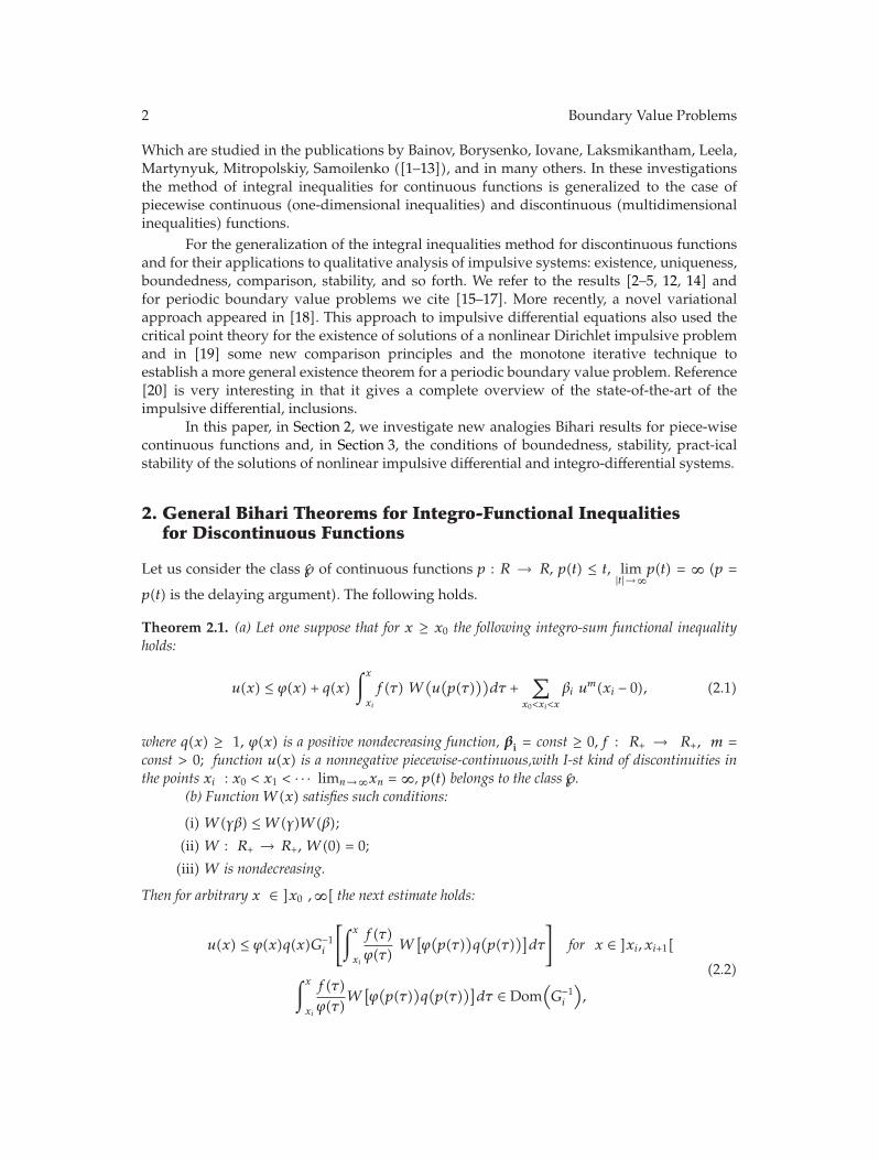
2. General Bihari Theorems for Integro-Functional Inequalitiesfor Discontinuous Functions
Let us consider the class ℘ of continuous functions p : R → R, p(t) ≤ t, lim|t|→∞
p(t) = ∞ (p =
p(t) is the delaying argument). The following holds.
Theorem 2.1. (a) Let one suppose that for x ≥ x0 the following integro-sum functional inequalityholds:
u(x) ≤ ϕ(x) + q(x)∫xxi
f(τ) W(u(p(τ)))dτ +
∑x0<xi<x
βi um(xi − 0), (2.1)
where q(x) ≥ 1, ϕ(x) is a positive nondecreasing function, βi = const ≥ 0, f : R+ → R+, m =const > 0; function u(x) is a nonnegative piecewise-continuous,with I-st kind of discontinuities inthe points xi : x0 < x1 < · · · limn→∞xn = ∞, p(t) belongs to the class ℘.
(b) FunctionW(x) satisfies such conditions:
(i) W(γβ) ≤W(γ)W(β);
(ii) W : R+ → R+, W(0) = 0;
(iii) W is nondecreasing.
Then for arbitrary x ∈ ]x0 ,∞[ the next estimate holds:
u(x) ≤ ϕ(x)q(x)G−1i
[∫xxi
f(τ)ϕ(τ)
W[ϕ(p(τ))q(p(τ))]dτ
]for x ∈ ]xi, xi+1[
∫xxi
f(τ)ϕ(τ)
W[ϕ(p(τ))q(p(τ))]dτ ∈ Dom
(G−1i
),
(2.2)
Boundary Value Problems 3
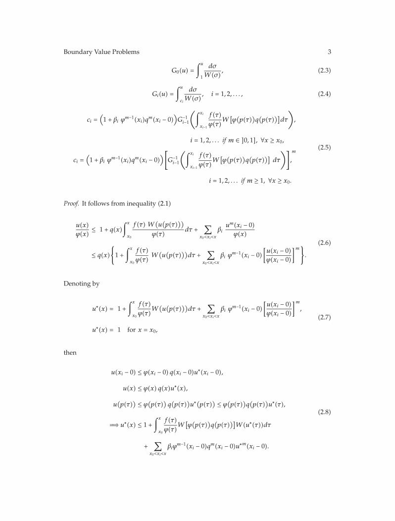
G0(u) =∫u1
dσ
W(σ), (2.3)
Gi(u) =∫uci
dσ
W(σ), i = 1, 2, . . . , (2.4)
ci =(1 + βi ϕm−1(xi)qm(xi − 0)
)G−1i−1
(∫xixi−1
f(τ)ϕ(τ)
W[ϕ(p(τ))q(p(τ))]dτ
),
i = 1, 2, . . . if m ∈ ]0, 1], ∀x ≥ x0,
ci =(1 + βi ϕm−1(xi)qm(xi − 0)
)[G−1i−1
(∫xixi−1
f(τ)ϕ(τ)
W[ϕ(p(τ))q(p(τ))]
dτ
)],
m
i = 1, 2, . . . if m ≥ 1, ∀x ≥ x0.
(2.5)
Proof. It follows from inequality (2.1)
u(x)ϕ(x)
≤ 1 + q(x)∫xx0
f(τ) W(u(p(τ)))
ϕ(τ)dτ +
∑x0<xi<x
βium(xi − 0)ϕ(x)
≤ q(x){1 +∫xx0
f(τ)ϕ(τ)
W(u(p(τ)))dτ +
∑x0<xi<x
βi ϕm−1(xi − 0)
[u(xi − 0)ϕ(xi − 0)
]m}.
(2.6)
Denoting by
u∗(x) = 1 +∫xx0
f(τ)ϕ(τ)
W(u(p(τ)))dτ +
∑x0<xi<x
βi ϕm−1(xi − 0)
[u(xi − 0)ϕ(xi − 0)
]m,
u∗(x) = 1 for x = x0,
(2.7)
then
u(xi − 0) ≤ ϕ(xi − 0) q(xi − 0)u∗(xi − 0),
u(x) ≤ ϕ(x) q(x)u∗(x),
u(p(τ)) ≤ ϕ(p(τ)) q(p(τ))u∗(p(τ)) ≤ ϕ(p(τ))q(p(τ))u∗(τ),
=⇒ u∗(x) ≤ 1 +∫xx0
f(τ)ϕ(τ)
W[ϕ(p(τ))q(p(τ))]W(u∗(τ))dτ
+∑
x0<xi<x
βiϕm−1(xi − 0)qm(xi − 0)u∗m(xi − 0).
(2.8)
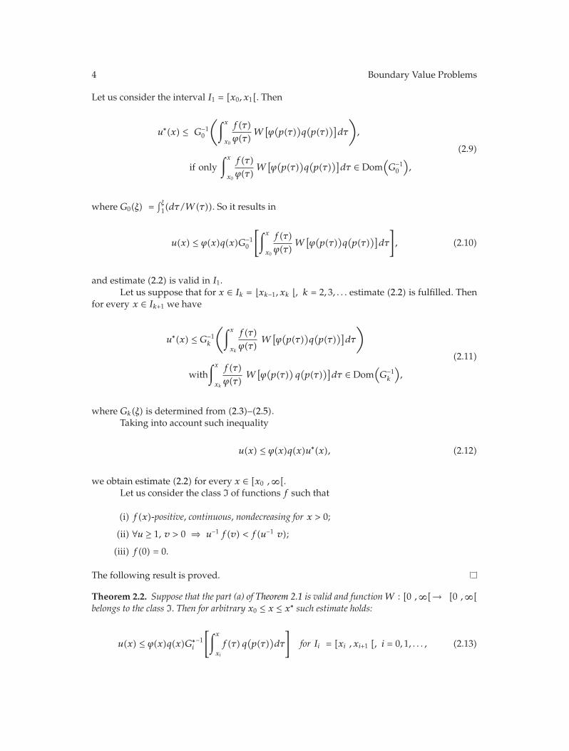
4 Boundary Value Problems
Let us consider the interval I1 = [x0, x1[. Then
u∗(x) ≤ G−10
(∫xx0
f(τ)ϕ(τ)
W[ϕ(p(τ))q(p(τ))]dτ
),
if only∫xx0
f(τ)ϕ(τ)
W[ϕ(p(τ))q(p(τ))]dτ ∈ Dom
(G−1
0
),
(2.9)
where G0(ξ) =∫ ξ1(dτ/W(τ)). So it results in
u(x) ≤ ϕ(x)q(x)G−10
[∫xx0
f(τ)ϕ(τ)
W[ϕ(p(τ))q(p(τ))]dτ
], (2.10)
and estimate (2.2) is valid in I1.Let us suppose that for x ∈ Ik = xk−1, xk , k = 2, 3, . . . estimate (2.2) is fulfilled. Then
for every x ∈ Ik+1 we have
u∗(x) ≤ G−1k
(∫xxk
f(τ)ϕ(τ)
W[ϕ(p(τ))q(p(τ))]dτ
)
with∫xxk
f(τ)ϕ(τ)
W[ϕ(p(τ))q(p(τ))]dτ ∈ Dom
(G−1k
),
(2.11)
where Gk(ξ) is determined from (2.3)–(2.5).Taking into account such inequality
u(x) ≤ ϕ(x)q(x)u∗(x), (2.12)
we obtain estimate (2.2) for every x ∈ [x0 ,∞[.Let us consider the class I of functions f such that
(i) f(x)-positive, continuous, nondecreasing for x > 0;
(ii) ∀u ≥ 1, v > 0 ⇒ u−1 f(v) < f(u−1 v);
(iii) f(0) = 0.
The following result is proved.
Theorem 2.2. Suppose that the part (a) of Theorem 2.1 is valid and functionW : [0 ,∞[→ [0 ,∞[belongs to the class I. Then for arbitrary x0 ≤ x ≤ x∗ such estimate holds:
u(x) ≤ ϕ(x)q(x)G∗i−1[∫x
xi
f(τ) q(p(τ))dτ
]for Ii = [xi , xi+1 [, i = 0, 1, . . . , (2.13)
Boundary Value Problems 5
where
G∗0(η)=∫η1
dσ
W(σ), G∗
i
(η)=∫ηc∗i
dσ
W(σ)i = 1, 2, . . . ,
c∗i =(1 + βi ϕm−1(xi)qm(xi)
)G∗i−1
−1(∫xi
xi−1f(τ)q
(p(τ))dτ
)if m ∈ ]0, 1],
c∗i =(1 + βi ϕm−1(xi)qm(xi)
)[G∗i−1
−1(∫xi
xi−1f(τ)q
(p(τ))dτ
)]mif m ≥ 1,
(2.14)
and x∗ = supx{∫xxi−1f(τ)q(p(τ))dτ ∈ Dom(G∗
i−1−1)}, i = 1, 2, . . . .
Proof. By using the previous theorem we have u(x) ≤ ϕ(x)g(x)u∗(x), u∗(x) = 1 x = x0. Onthe interval I1
du∗(x)dx
=f(x)ϕ(x)
W(u(p(x))). (2.15)
Then
u(p(x)) ≤ ϕ(p(x))q(p(x))u∗(p(x)) ≤ ϕ(x)q(p(x))u∗(x),
du∗(x)dx
≤ f(x)ϕ(x)
W(q(p(x))ϕ(x)u∗(x)
)
≤ f(x)q(p(x))
ϕ(x)q(p(x))W(q(p(x))ϕ(x)u∗(x))
≤ f(x)q(p(x))W(u∗(x)).
(2.16)
Taking into account estimate (2.16), we obtain
∫xx0
u∗′(σ)W(u∗(σ))
dσ ≤∫xx0
f(τ)q(p(τ))dτ,
∫xx0
u∗′(σ)W(u∗(σ))
dσ =∫u∗(x)u∗(x0)
du
W(u)= G∗
0(u∗(x)) −G∗
0(u∗(x0)),
u∗(x0) = 1, u∗(x) ≥ 1, G∗0(u
∗(x0)) = G∗0(1) = 0,
G∗0(u
∗(x)) ≤∫xx0
f(τ) q(p(τ))dτ.
(2.17)
6 Boundary Value Problems
Then in I1 we have
u(x) ≤ ϕ(x)q(x) G∗0−1[∫x
x0
f(τ)q(p(τ))dτ
]if only
∫xx0
f(τ)q(p(τ))dτ ∈ Dom
(G∗
0−1).(2.18)
As in the previously theorem, the proof is completed by using the inductive method.
The following result is easily to obtain
Theorem 2.3. Suppose that for x ≥ x0 the next inequality holds:
u(x) ≤ u0 + q(x)[∫x
x0
f(s)u(p(s))ds +∫xx0
f(s)
(∫xx0
g(τ)u(p(τ))dτ
)ds
]
+∫xx0
h(s)W(u(σ(s)))ds +∑
x0<xi<x
βi um(xi − 0),
(2.19)
where functions u(x), f(x), q(x), g(x), h(x), p(x), σ(x) are real nonnegative for x ≥ x0 >0, p(x), σ(x) ∈ I, q(x) ≥ 1, βi ≥ 0, function W satisfies conditions (i),. . .,(iii) of Theorem 2.1.
Then for x ≥ x0 it results in
u(x) ≤∏
x0<xi<x
(1 + βiqm(xi)um−1
0
)exp
(∫xx0
q(p(τ))[f(τ) + g(τ)
]dτ
)
· ψ−10
⎛⎝∫xx0
h(τ) W
⎡⎣ ∏x0<xi<σ(τ)
(1 + βiqm(xi)um−1
0
)⎤⎦W
×[q(σ(τ)) exp
(∫σ(τ)x0
q(p(s))[f(s) + g(s)
]ds
)]dτ
), if m ∈ ]0, 1]
∫xx0
h(τ)W
⎡⎣ ∏x0<xi<σ(τ)
(1 + βiqm(xi)um−1
0
)⎤⎦W
×[q(σ(τ)) exp
(∫σ(τ)x0
q(p(s))[f(s) + g(s)
]ds
)]dτ ∈ Dom
(ψ−10
),
(2.20)

Boundary Value Problems 7
where ψ0(u) =∫uu0(dv/W(v));
u(x) ≤∏
x0<xi<x
(1 + βiqm(xi)um−1
0
)exp
(m
∫xx0
q(p(τ))[f(τ) + g(τ)
])
· ψ−10
⎛⎝∫xx0
h(τ)
⎡⎣ ∏x0<xi<σ(τ)
(1 + βiqm(xi)um−1
0
)⎤⎦
·W[q(σ(τ)) exp
(m
∫σ(τ)x0
q(p(s))[f(s) + g(s)
]ds
)]dτ
), if m ≥ 1,
∫xx0
h(τ)W
⎡⎣ ∏x0<xi<σ(τ)
(1 + βiqm(xi)um−1
0
)⎤⎦W
×[q(σ(τ)) exp
(m
∫σ(τ)x0
q(p(s))[f(s) + g(s)
]ds
)]dτ ∈ Dom
(ψ−10
).
(2.21)
The proof the same procedure as that of (Iovane [21, Theorems 2.1 and 3.1]).
Corollary 2.4. Suppose that
(a) m = 1, then the result of Theorem 2.1 coincides with the result [22, Theorem 3.7.1, page232];
(b) m = 1, ϕ(x) = c, q(x) = 1, p(t) = t, then the result of Theorem 2.1 coincides with result[12, Proposition 2.3, page 2143];
(c) q(x) = 1, W(u) = u, p(t) = t, then one obtains the analogy of Gronwall- Bellman resultfor discontinuous functions [23, Lemma 1] and estimate (2.2) reduces in the following form:
u(x) ≤ ϕ(x)∏
x0<xi<x
(1 + βi ϕm−1(xi)
)exp
(∫xx0
f(τ) dτ
)if m ∈ ]0, 1], ∀x ≥ x0,
u(x) ≤ ϕ(x)∏
x0<xi<x
(1 + βi ϕm−1(xi)
)exp
(m
∫xx0
f(τ) dτ
)if m ≥ 1, ∀x ≥ x0.
(2.22)
(d) q(x) = 1, W(u) = u, then one obtains the result [21, Theorem 2.1] and estimate (2.2) areas follows:
u(x) ≤ ϕ(x)∏
x0<xi<x
(1 + βi ϕm−1(xi)
)exp
(∫xx0
f(τ)ϕ(p(τ))
ϕ(τ)dτ
), if m ∈ ]0, 1], ∀x ≥ x0;
u(x) ≤ ϕ(x)∏
x0<xi<x
(1 + βi ϕm−1(xi)
)exp
(m
∫xx0
f(τ)ϕ(p(τ))
ϕ(τ)dτ
)if m ≥ 1, ∀x ≥ x0.
(2.23)
8 Boundary Value Problems
(e) q(x) = 1,W(u) = um,m > 0, p(t) = t, then one obtains the analogy of Bihari result fordiscontinuous functions [23, Lemma 2] and estimate (2.2) reduces as follows are reduced:
u(x) ≤ ϕ(x)∏
x0<xi<x
(1 + βi ϕm−1(xi)
)[1 + (1 −m)
∫xx0
ϕm−1(τ)f(τ)dτ
]1/(1−m)
,
if 0 < m < 1, ∀x ≥ x0,
u(x) ≤ ϕ(x)∏
x0<xi<x
(1 + βimϕm−1(xi)
) ⎡⎣1 − (m − 1)
[ ∏x0<xi<x
(1 + βi mϕm−1(xi)
)]m−1
×∫xx0
ϕm−1(τ) f(τ) dτ
]− 1/(m−1)∀x ≥ x0,
(2.24)
such that
∫xx0
ϕm−1(τ)f(τ) dτ ≤ 1m, m > 1,
∏x0<xi<x
(1 + βi ϕm−1(xi)
)<
(1 +
1m − 1
)1/(m−1).
(2.25)
(f) W(u) = um,, m> 0, then estimate (2.2) reduces as follows (see [21, Theorem 2.2]):
u(x) ≤ ϕ(x) q(x)∏
x0<xi<x
(1 + βi ϕm−1(xi) qm(xi)
)
×[1 + (1 −m)
∫xx0
ϕm−1(τ)f(τ)qm(p(τ))[ϕ(p(τ))
ϕ(τ)
]mdτ
]1/(1−m)
if 0 < m < 1, ∀x ≥ x0,
u(x) ≤ ϕ(x) q(x)∏
x0<xi<x
(1 + βimϕm−1(xi) qm(xi)
)
×⎧⎨⎩1 − (m − 1)
[ ∏x0<xi<x
(1 + βi mϕm−1(xi)qm(xi)
)]m−1
×∫xx0
ϕm−1(τ) f(τ)qm(p(τ))[ϕ(p(τ))
ϕ(τ)
]mdτ
}− 1/(m−1)∀x ≥ x0
Boundary Value Problems 9
such that
∫xx0
ϕm−1(τ) f(τ)qm(p(τ))[ϕ(p(τ))
ϕ(τ)
]mdτ ≤ 1
m, m > 1,
∏x0<xi<x
(1 + βimϕm−1(xi)qm(xi)
)<
(1 +
1m − 1
)−1/(m−1).
(2.26)
(g) Suppose that in Theorem 2.3 q(x) = 1,W(u) = u, σ(s) = p(s) = s, then estimates (2.20),(2.21) reduce as shown:
u(x) ≤ u0∏
x0<xi<x
(1 + βi um−1
0 (xi))exp
[∫xx0
[f(ξ) + g(ξ) + h(ξ)
]dξ
]if m ∈ ]0, 1], ∀x ≥ x0;
u(x) ≤ u0∏
x0<xi<x
(1 + βi um−1
0 (xi))exp
[m
∫xx0
[f(ξ) + g(ξ) + h(ξ)
]dξ
]if m ≥ 1, ∀x ≥ x0,
(2.27)
which coincide with result of [21, Theorem 3.1] for h(t) = u0.
3. Applications
Let us consider the following system of differential equations
dx
dt= F(t, x), t /= ti,
Δx|t=ti = Ii(x)(3.1)
where x ∈ Rn, F ∈ Rn, Ii(x) ∈ Rn (i = 1, 2, . . .), t ≥ t0 ≥ 0, limi→∞ ti = ∞, ti−1 < ti for all i =1, 2, . . ..
Let us assume that F(t, x) and Ii(x) are defined in the domain D = {(t, x) : t ∈ I =[t0, T], T ≤ ∞, ‖x‖ ≤ h } and satisfy such conditions:
(a) ‖F(t, x)‖ ≤ f(t)W(‖x‖), f : R+ → R+,
W satisfies conditions (i)–(iii) of Theorem 2.1;
(b) ‖Ii(x) ‖ ≤ βi‖x‖m, βi = const > 0, m > 0.
Consider x(t) = x( t, t0, x0) the solution of Cauchy problem for system (3.1). Then
x(t, t0, x0 ) = x0 +∫ tt0
F(τ, x(τ, t0, x0))dτ +∑t0<ti<t
Ii(x(ti − 0, t0, x0)), (3.2)
10 Boundary Value Problems
from which it follows
‖x(t, t0, x0 )‖ ≤ ‖x0‖ +∫ tt0
f(τ) W(‖x(τ, t0, x0)‖)dτ +∑t0<ti<t
βi‖x(ti − 0, t0, x0)‖m. (3.3)
By using the result of Theorem 2.1 and estimate (2.2) we obtain
‖x(t, t0, x0)‖ ≤ ‖x0‖G−1i
[∫xxi
f(τ)W(‖x0‖)‖x0‖ dτ
]for x ∈ ]xi, xi+1[ ,
∫xxi
f(τ)W(‖x0‖)‖x0‖ dτ ∈ Dom
(G−1i
),
(3.4)
where
G0(u) =∫u1
dσ
W(σ), Gi(u) =
∫uci
dσ
W(σ), i = 1, 2, ...,
ci =(1 + βi‖x0‖m−1
)G−1i−1
(∫xixi−1f(τ)
W(‖x0‖)‖x0‖ dτ
),
i = 1, 2, . . . if m ∈ ]0, 1], ∀x ≥ x0,
ci =(1 + βi‖x0‖m−1
)[G−1i−1
(∫xixi−1f(τ)
W(‖x0‖)‖x0‖ dτ
)]m,
i = 1, 2, . . . if m ≥ 1, ∀x ≥ x0.
(3.5)
Let us consider some particular cases ofW .IfW(u) = u, m = 1, estimate (3.4) is reduced in such form
‖x(t, t0, x0)‖ ≤ ‖x0‖∏t0<ti<t
(1 + βi
)exp
[∫ tt0
f(τ)dτ
]. (3.6)
Then such result holds.
Proposition 3.1. Let the following conditions be fulfilled for system (3.1) :
(i) ‖F(t, x)‖ ≤ f(t)‖x‖;(ii) ‖Ii(x)‖ ≤ βi‖x‖;(iii) ∃m1(t0) = const. > 0 :
∏t0<ti<t
(1 + βi) ≤ m1(t0) <∞;
(iv) ∃m2(t0) = const. > 0 :∫ tt0f(τ) dτ ≤ m2(t0) <∞, ∀t ≥ t0 .
Boundary Value Problems 11
Then one has:
(a) All solutions of system (3.1) are bounded (uniformly, if mi(t0) are independent of t0) andsuch estimate is valid:
‖x(t, t0, x0)‖ ≤ m1(t0) exp[m2(t0)]‖x0‖. (3.7)
(b) The trivial solution of system (3.1) is stable by Lyapunov (uniformly stable relative t0, ifmi(t0) = mi, i = 1, 2).
Remark 3.2. If conditions I–IV of Proposition 3.1 are valid and λ/Λ < (m1(t0) exp[m2(t0)])−1,
then the trivial solution is (λ,Λ, I)-stable by Chetaev (uniformly (λ,Λ, I)-stable, if mi(t0),i = 1, 2 is independent of t0).
IfW(u) = ul, l /= 1, m = 1 the estimate (3.4) is reduced in such form
‖x(t, t0, x0)‖ ≤∏t0<ti<t
(1 + βi
)[‖x0‖1−l + (1 − l)∫ tt0
f(τ)dτ
]1/(1−l)∀t ≥ t0, if 0 < l < 1, (3.8)
‖x(t, t0, x0)‖ ≤ ‖x0‖∏t0<ti<t
(1 + βi
)
×⎡⎣1 − (l − 1) ‖x0‖l−1 ·
[∏t0<ti<t
(1 + βi
)]l−1∫ tt0
f(τ)dτ
⎤⎦
− 1/(l−1)
∀t ≥ t0,(3.9)
∫ tt0
f(τ)dτ <
⎛⎝(l − 1)
[‖x0‖
∏t0<ti<t
(1 + βi
) ]l−1⎞⎠
−1
, if l > 1. (3.10)
From estimate (3.8) the next propositions follow.
Proposition 3.3. Suppose that such conditions occur:
(a) ‖F(t, x) − F(t, y)‖ ≤ f(t) ‖x − y‖l, 0 < l < 1 for allx, y ∈ D(b) estimates ii–iv of Proposition 3.1 be fulfilled.
Then all the solutions of system (3.1) are bounded (uniformly ifmi(t0) = mi, i = 1, 2).
Remark 3.4. Suppose that conditions (a), (b) of Proposition 3.3 are valid and
λ1−l + (1 − l) m2(t0) <[
Λm1(t0)
]1−l. (3.11)
12 Boundary Value Problems
Then trivial solution of system (3.1) is (λ,Λ, I)-stable by Chetaev (uniformly if mi(t0) isindependent of t0).
Proposition 3.5. Let conditions ii–iv of Proposition 3.1 be fulfilled for system (3.1), inequality (3.10)holds and
‖F(t, x)‖ ≤ f(t)‖x ‖l, l > 1. (3.12)
Then trivial solution of system (3.1) is stable by Lyapunov (uniformly ifmi(t0) = mi, i = 1, 2).
Remark 3.6. IfW(u) = u1, 1 > 0, and m/= 1 the conditions of boundedness, stability, (λ,Λ, I)-stability is investigated in [14, see Theorems 3.4–3.6]; the estimates of the solutions of system(3.1) with non-Lipschitz type of discontinuities are investigated in [23, see Proposition 1,Proposition 2].
Let us consider the following impulsive system of integro-differential equations:
dx
dt= F(t, x,K[x(t)]), t /= ti,
Δx|t=ti = Ii(x),(3.13)
where x ∈ Rn, F ∈ Rn, Ii(x) ∈ Rn (i = 1, 2, . . .) and defined in the domain D, K[x(t)] =∫ tt0k(t, τ, x(τ)) dτ .
We suppose that such conditions are valid:
(i) ‖F(t, x, y)‖ ≤ f(t)[‖x‖ + ‖y‖] for allx, y ∈ D, f : R+ → R+;
(ii) ‖k(t, s, x)‖ ≤ g(t)‖x‖ for all s ∈ [t0, t], g : R+ → R+;
(iii) ‖Ii(x)‖ ≤ βi‖x‖m for allx, y ∈ D, βi = const > 0, m > 0 m/= 1.
It is easy to see that
‖x(t, t0, x0 )‖ ≤ ‖x0‖ +∫ tt0
f(τ)‖x(τ, t0, x0)‖dτ
+∫ tt0
f(τ)
(∫ τt0
g(ξ)‖x(ξ, t0, x0)‖dξ)dτ +
∑t0<ti<t
βi‖x(ti − 0, t0, x0)‖m
=⇒ ‖x(t, t0, x0)‖ ≤ ‖x0‖∏t0<ti<t
(1 + βi‖x0‖m−1
)exp∫ tt0
[f(ξ) + g(ξ)
]dξ,
if 0 < m ≤ 1, t ≥ t0
(3.14)
‖x(t)‖ ≤ ‖ x0‖∏t0<ti<t
(1 + βi‖x0‖m−1
)exp
(m
∫ tt0
[f(ξ) + g(ξ)
]dξ
),
if 0m ≥ 1, t ≥ t0.(3.15)
From estimate (3.15) such result follows.
Boundary Value Problems 13
Proposition 3.7. Let one suppose that for system (3.13) conditions (i)–(iii) take place for m > 1 andthe following estimates are fulfilled:
(a) ∃ m3(t0) = const. > 0 :∏
t0<ti<t(1 + βi‖x0‖m−1) ≤ m3(t0) <∞;
(b) ∃ m4(t0) = const. > 0 :∫ tt0[f(ξ) + g(ξ)] dξ ≤ m4(t0) <∞ for all t ≥ t0.
Then we have:
(i) All solutions of system (3.13) are bounded and satisfy the estimate:
‖x(t)‖ ≤ m3(t0) exp[m4(t0)]‖x0‖. (3.16)
(ii) The trivial solution of system (3.13) is stable by Lyapunov (uniformly, ifmi(t0) = mi, i =3, 4).
(iii) The trivial solution of system (3.13) is (λ,Λ, I)-stable by Chetaev (uniformly if mi(t0) isindependent of t0) andm3(t0) exp[m4(t0)] < Λ/λ.
References
[1] D. Banov and P. Simeonov, Integral Inequalities and Applications, vol. 57 of Mathematics and ItsApplications, Kluwer Academic Publishers, Dordrecht, The Netherlands, 1992.
[2] S. D. Borysenko, G. Iovane, and P. Giordano, “Investigations of the properties motion for essentialnonlinear systems perturbed by impulses on some hypersurfaces,”Nonlinear Analysis: Theory, Methods& Applications, vol. 62, no. 2, pp. 345–363, 2005.
[3] S. D. Borysenko, M. Ciarletta, and G. Iovane, “Integro-sum inequalities and motion stability ofsystems with impulse perturbations,” Nonlinear Analysis: Theory, Methods & Applications, vol. 62, no.3, pp. 417–428, 2005.
[4] S. Borysenko and G. Iovane, “About some new integral inequalities of Wendroff type fordiscontinuous functions,” Nonlinear Analysis: Theory, Methods & Applications, vol. 66, no. 10, pp. 2190–2203, 2007.
[5] S. C. Hu, V. Lakshmikantham, and S. Leela, “Impulsive differential systems and the pulsephenomena,” Journal of Mathematical Analysis and Applications, vol. 137, no. 2, pp. 605–612, 1989.
[6] V. Lakshmikantham and S. Leela, Differential and Integral Inequalities, Theory and Applications,Academic Press, New York, NY, USA, 1969.
[7] V. Lakshmikantham, S. Leela, and M. Mohan Rao Rama, “Integral and integro-differentialinequalities,” Applicable Analysis, vol. 24, no. 3, pp. 157–164, 1987.
[8] V. Lakshmikantham, D. D. Bainov, and P. S. Simeonov, Theory of Impulsive Differential Equations, vol. 6of Series in Modern Applied Mathematics, World Scientific, Teaneck, NJ, USA, 1989.
[9] A. A. Martyhyuk, V. Lakshmikantham, and S. Leela, Stability of Motion: the Method of IntegralInequalities , Naukova Dumka, Kyiv, Russia, 1989.
[10] Yu. A. Mitropolskiy, S. Leela, and A. A. Martynyuk, “Some trends in V. Lakshmikantham’sinvestigations in the theory of differential equations and their applications,” Differentsial’nyeUravneniya, vol. 22, no. 4, pp. 555–572, 1986.
[11] Yu. A. Mitropolskiy, A. M. Samoilenko, and N. Perestyuk, “On the problem of substantiation ofoveroging method for the second equations with impulse effect,” Ukrainskii Matematicheskii Zhurnal,vol. 29, no. 6, pp. 750–762, 1977.
[12] Yu. A. Mitropolskiy, G. Iovane, and S. D. Borysenko, “About a generalization of Bellman-Bihari typeinequalities for discontinuous functions and their applications,” Nonlinear Analysis: Theory, Methods& Applications, vol. 66, no. 10, pp. 2140–2165, 2007.
[13] A. M. Samoilenko and N. Perestyuk, Differential Equations with Impulse Effect, Visha Shkola, Kyiv,Russia, 1987.
14 Boundary Value Problems
[14] A. Gallo and A. M. Piccirillo, “About new analogies of Gronwall-Bellman-Bihari type inequalitiesfor discontinuous functions and estimated solutions for impulsive differential systems,” NonlinearAnalysis: Theory, Methods & Applications, vol. 67, no. 5, pp. 1550–1559, 2007.
[15] J. J. Nieto, “Impulsive resonance periodic problems of first order,” Applied Mathematics Letters, vol. 15,no. 4, pp. 489–493, 2002.
[16] J. J. Nieto, “Basic theory for nonresonance impulsive periodic problems of first order,” Journal ofMathematical Analysis and Applications, vol. 205, no. 2, pp. 423–433, 1997.
[17] J. J. Nieto, “Periodic boundary value problems for first-order impulsive ordinary differentialequations,” Nonlinear Analysis: Theory, Methods & Applications, vol. 51, no. 7, pp. 1223–1232, 2002.
[18] Z. Luo and J. J. Nieto, “New results for the periodic boundary value problem for impulsive integro-differential equations,”Nonlinear Analysis: Theory, Methods &Applications, vol. 70, no. 6, pp. 2248–2260,2009.
[19] J. J. Nieto and D. O’Regan, “Variational approach to impulsive differential equations,” NonlinearAnalysis: Real World Applications, vol. 10, no. 2, pp. 680–690, 2009.
[20] M. Benchohra, J. Henderson, and S. Ntouyas, Impulsive Differential Equations and Inclusions, vol. 2 ofContemporary Mathematics and Its Applications, Hindawi Publishing Corporation, New York, NY, USA,2006.
[21] G. Iovane, “Some new integral inequalities of Bellman-Bihari type with delay for discontinuousfunctions,” Nonlinear Analysis: Theory, Methods & Applications, vol. 66, no. 2, pp. 498–508, 2007.
[22] A. Samoilenko, S. Borysenko, C. Cattani, G. Matarazzo, and V. Yasinsky, Differential Models: Stability,Inequalities and Estimates, Naukova Dumka, Kiev, Russia, 2001.
[23] D. S. Borysenko, A. Gallo, and R. Toscano, “Integral inequalities Gronwall-Bellman type fordiscontinuous functions and estimates of solutions impulsive systems,” in Proc.DE@CAS, pp. 5–9,Brest, 2005.