On Optimal Boundary and Distributed Control of Partial Integro-Differential Equations. Об...

Archives of Control SciencesVolume 24(LX), 2014

No. 1, pages 5–25

On optimal boundary and distributed control of partialintegro–differential equations

ASATUR ZH. KHURSHUDYAN

To memoriam of my father Zhora M. Khurshudyan is dedicated.

A method of optimal control problems investigation for linear partial integro–differentialequations of convolution type is proposed, when control process is carried out by boundaryfunctions and right hand side of equation. Using Fourier real generalized integral transformcontrol problem solution is reduced to minimization procedure of chosen optimality criterionunder constraints of equality type on desired control function. Optimality of control impactsis obtained for two criteria, evaluating their linear momentum and total energy. Necessary andsufficient conditions of control problem solvability are obtained for both criteria. Numericalcalculations are done and control functions are plotted for both cases of control process realiza-tion.

Key words: optimal control, integro–differential equation, equation of convolution type,Fourier generalized transform, impulsive control

1. Introduction

It is well known fact that the most part of rigorous techniques of optimal control sys-tems investigation are non–applicable for solution of control problems for some specialtypes of system uncertainties, and application of existing efficient numerical methodsin those situations is quite onerous. For example, when the system of optimal controlis nonlinear with respect to control vector (and even linear with respect to phase vec-tor), the problem can be solved explicitly only in some exceptional cases, and problemsof control by coefficients or by moving loads are rigorously irresolvable [1, 2]. Thereare many other examples of control problems, when system‘s investigation is associatedwith additional difficulties and costs. Quite a common example of control system withuncertainty is a system containing convolution of unknown function, which occurs invarious areas of mathematical physics and includes integral (Fredholm equations of thefirst and second kinds), as well as integro–differential equations (in ordinary and partialderivatives).

A.Z. Khurshudyan is with Faculty of Mathematics and Mechanics, Yerevan State University, AlexManoogian Str. 1, 0025 Yerevan, Armenia, email: [email protected]

Research was carried out during SISSA (Trieste, Italy) fellowship.Received 13.01.2014. Revised 4.03.2014.

6 A.Z. KHURSHUDYAN

Many real processes are very often roughly modeled by ordinary or partial differ-ential equations. However, local character of differential equations does not allow us totake into account such real–world phenomena, as, for instance, processes with memory(prehistory). Introduction of integral terms containing unknown function into differen-tial equation, thereby transforming it into integro–differential, is of help in this case. Asa common example of such equations in finite interval, the following one may serve (inone dimensional case):

H [w]+b∫

a

K (x,s, t)N [w]ds = F (x, t), (1)

where w = w(x, t) is the unknown function, K : [a,b]× [a,b]×T→ R is a given func-tion, called kernel of equation, T is finite or infinite interval, H [·] and N [·] are differ-ential operators, acting on unknown function, and F : [a,b]×T→ R is the given righthand side, satisfying certain conditions. If operators H [·] and N [·] are linear, containsordinary or partial derivatives, then equation (1) is called linear, ordinary or partial, re-spectively. Furthermore, equation (1) is called symmetric, if its kernel is symmetric:K (x,s, ·) = K (s,x, ·), and difference or convolution type, if K (x,s, ·) = K (x− s, ·).

The monograph [3] is devoted to thorough investigation and classification of integro–differential operators. Main areas of integro–differential equations application are de-scribed, and numerous problems mathematically formulated by those equations, partic-ularly in theories of elasticity and viscoelasticity, continuum mechanics, contact interac-tions mechanics, growing body mechanics and fracture mechanics are considered ibid.In [4] the description of some financial processes by partial integro–differential equa-tions are investigated. In [5] the explicit solution of linear difference partial integro–differential equations in quite general form is obtained via Laplace transform. Someexamples of integro–differential equations occurring in applications are solved and in-vestigated. Numerical method of nonlinear singular partial integro–differential equationssolution is constructed in [6].

Accounting of such irreversible processes of wave energy transfer to medium par-ticle as dispersion and dissipation, is accompanied with introduction in ordinary waveequation of some additional linear terms containing the unknown function, the form ofwhich depends only on physical mechanism of interaction between wave and medium.In general, the description of wave propagation in a homogeneous isotropic mediumwith dissipation or dispersion properties occupied domain Ω ⊂ R3 in 3–dimensionalformulation is mathematically equivalent to solution of the following wave equation:

∆w =1c2

∂2w∂t2 +L [w], (x,y,z) ∈Ω, t > 0, (2)

where w = w(x,y,z, t) is the unknown function, ∆ is 3–dimensional Laplace operator,and L [w] is some linear operator, acting on function w(x,y,z, t). Particularly, in sound

OPTIMAL CONTROL OF PARTIAL INTEGRO–DIFFERENTIAL EQUATIONS 7

wave propagation problem in a dissipative medium [7]

L [w]≡− bc2

0ρ0

∂2∆w∂t2 ,

where b is the medium dissipation factor. In propagation problem of electromagneticwave in a dispersive medium [7]

L [w]≡ 4πc2

1

∂2

∂t2

∞∫0

κ(τ)w(x,y,z, t− τ)dτ, (3)

where κ(t), t > 0, is a dimensionless bounded function, characterizing dielectric suscep-tibility of medium. Typical examples of electromagnetic waves include radio waves, TVsignals, radar beams, and light rays.

It turns out, that taking into account such simple (in the sense of linearity), but nat-ural phenomena considerably complicates the investigation, and numerical calculationsmakes more time consuming. Investigation of control problems for such systems is alsoextremely complicated.

The main purpose of this investigation is development of optimal control problemsolution technique namely for such systems, when control process is carried out by aboundary function and right hand side of equation. Simplicity of numerical applicationof technique is also one of our aims. Taking into consideration the uncertainty typeof those equations, one may easily see, that control algorithm to be developed shouldbe based on some integral transform. Optimal control problems for integro–differentialequations are considered also in [8, 9, 10, 11].

2. Mathematical statement of the problem

So, we begin our investigation with non–homogeneous, one–dimensional analogueof equation (2) in finite interval (for simplicity, symmetric: it can always be done bylinear transformation of variable t) when (3) is taken into account:

∂2w∂x2 =

∂2w∂t2 +α

∂2

∂t2

θ∫−θ

κ(τ)w(x, t− τ)dτ+U(x, t), (4)

(x, t) ∈ (0,1)× (−θ,θ),

where α ∈ R+ is a dimensionless constant, subjected to boundary conditions

w(0, t) = φ(t), w(l, t) = ψ(t), t ∈ (−θ,θ), (5)

(all quantities and variables are dimensionless).

8 A.Z. KHURSHUDYAN

From mathematics point of view, control process of system (4)–(5) may be carriedout either by one of boundary functions φ(t) and ψ(t), or by function U(x, t) from righthand side of equation (4). The case when control process is realized by function κ(t) isconsiderably difficult. Let us suppose for definiteness, that [12, 13] U(x, t) = p(x)u(t),where p(x) is a given nonzero function, and control process may be realized by functionu(t).

The following initial data at t =−θ and terminal data at t = θ are considered:

w(x,−θ) = w−θ(x),∂w(x, t)

∂t

∣∣∣∣t=−θ

= w−θ(x), x ∈ (0,1), (6)

w(x,θ) = wθ(x),∂w(x, t)

∂t

∣∣∣∣t=θ

= wθ(x), x ∈ (0,1). (7)

In the framework of accepted physical interpretation system (4)–(5), in particular,describes the transfer of one–dimensional electromagnetic signal (impulse) on a finitedistance in dispersive medium, at that φ(t) and ψ(t) are input and output signals, re-spectively. Then, unlike traditional statement of optimal control problems for distributedparameter systems [1], demanding ensuring of given terminal data for given initial ones,we may demand to ensure one boundary condition by appropriate choice of the otherone when functions (6), (7) are given.

The main purpose of this investigation is to construct an efficient for numerical rea-sons algorithm of the following two problems solution.

The first problem or the problem of boundary control requires determination of afunction φo(t) optimal in the sense of given optimality criterion among all admissiblecontrols φ ∈ D ensuring given output signal ψ(t) when data (6) and (7) are given, andfind necessary and sufficient conditions of its existence.

The second problem or the problem of distributed control requires determination ofa function uo(t) optimal in the sense of given optimality criterion among all admissiblecontrols u∈D ensuring given output signal ψ(t) when input signal φ(t) and data (6) and(7) as well, are given, as well as find necessary and sufficient conditions of its existence.

Hereafter, we shall call a real–valued function admissible control, if it satisfies thesystem (4)–(6) solution existence and uniqueness conditions in considered functionspace. Further, we shall call a controlled system fully controllable in a certain space,if there exists an admissible control function, resolving the first or second problems forthat system in that space [12]– [14].

Further, in order to write equation (4) for all real t, let us introduce operator Aθ[·]defined on whole real axis and acting as

Aθ[ f (·, t)] =

f (·, t), t ∈ [−θ,θ];0, t /∈ [−θ,θ].


The explicit form of operator Aθ[·] can be constructed in several manners. For example,it can be done using characteristic function (indicator) of segment [−θ,θ]:

χ[−θ,θ](t) =

1, t ∈ [−θ,θ];0, t /∈ [−θ,θ].

Indeed, it is obvious, that Aθ[ f ] = χ[−θ,θ](t) f (·, t). Expressing characteristic functionχ[−θ,θ](t) in terms of Heaviside unit–step function, defined as

H(t) =

1, t > 0;0, t < 0,

we can write operator Aθ[·] as follows:

Aθ[ f (·, t)] = [H(t +θ)−H(t−θ)] f (·, t)≡ f1(·, t), t ∈ R.

Then using this expression, one can write equation (2.1) in space of generalized functionsfor all real t, and include initial and terminal data (2.3), (2.4) in it:

∂2w1

∂x2 =∂2w1

∂t2 +α∂2

∂t2 [κ1 ∗w1]+U1(x, t)+W (x, t), (x, t) ∈ [0,1]×R, (8)

W (x, t) =W−(x, t)−W+(x, t),

W±(x, t) = [δ(t±θ)+ακ1(t±θ)]w±θ(x)+ddt[δ(t±θ)−ακ1(t±θ)]w±θ(x),

where δ(t) is the Dirac delta function, defined as

δ(t) = H ′(t) =

0, t = 0;∞, t = 0,

at that∞∫−∞

δ(t)dt = 1, δ(−t) = δ(t),

with derivativedδ(t)

dt= δ′(t),

which is taken in generalized sense [15]. It should be noted, that function W (x, t) con-taining delay and advance of argument t is identically zero when t±θ /∈ [−θ,θ], at that

W (x, t) =

−W+(x, t), t ∈ [−θ,0);W0(x), t = 0;W−(x, t), t ∈ (0,θ],

x ∈ [0,1],

10 A.Z. KHURSHUDYAN

where

W0(x) = α[κ1(−θ)w−θ(x)−κ′1(−θ)w−θ(x)−κ1(θ)wθ(x)+κ′1(θ)wθ(x)

].

When obtaining right hand side of equation (8) the following relation was used [15]:

f (t)δ′(t−θ) = f (θ)δ′(t−θ)− f ′(θ)δ(t−θ).

Symbol ∗ in right hand side of equation (8) denotes operator of convolution acting asfollows:

κ1 ∗w1 =

∞∫−∞

κ1(τ)w1(x, t− τ)dτ =∞∫−∞

κ1(t− τ)w1(x,τ)dτ.

In transformed form equation (8) often occurs also in optics, mechanics and theoryof probability [17, 16, 7].

In the same way from boundary conditions (5) we will obtain

w1(0, t) = φ1(t), w1(1, t) = ψ1(t), t ∈ R. (9)

3. Boundary control

It is obvious that functions w1(x, t), φ1(t), ψ1(t) and U1(x, t) are defined for all t ∈Rand identically zero outside interval [−θ,θ], i.e. are compactly supported in that interval,where they coincide with functions w(x, t), φ(t), ψ(t) and U(x, t).

Applying now Fourier real generalized integral transform with respect to variable tin the sense of [15] to equation (8) and conditions (9), using the formulae of convolutiontransform, after some algebraic transformations we will obtain:

d2w1(x,σ)dx2 +σ2[1+ακ1(σ)]w1(x,σ) =U1(x,σ)+W (x,σ), (10)

(x,σ) ∈ (0,1)×R,w1(0,σ) = φ1(σ), w1(1,σ) = ψ1(σ),

where

Ft [ f (·, t)]≡ f (·,σ) =∞∫−∞

f (·, t)eiσtdt, σ ∈ R,

is the Fourier real generalized transform, at that

Ft [g1(·, t)] = FtAθ[g(·, t)]=θ∫−θ

g(·, t)eiσtdt, σ ∈ R,

Ft [·] is the Fourier operator, and σ is the spectral parameter of Fourier transform.Solution of the first problem gives the following


Theorem 1 Function φ1(t) ∈D is the Fourier inverse transform of function φ1(z), z =σ+ iς, determining from countable system

φ1(zk) = [ψ1(zk)−Φ(zk)]eχ(zk), k = 1,2,3, ..., (11)

where complex numbers zk are determined from characteristic equation

e2χ(z) = 1. (12)

Hereχ(z) = i

√z2 +αz2κ1(z),

Φ(z) =1

χ(z)

1∫0

[U1(ξ,z)+W (ξ,z)

]sinh[(1−ξ)χ(z)]dξ.

From Theorem 1 immediately follows

Corollary 1 If kernel κ1(t) of equation (8) satisfies conditionsa) Ft [κ1(t)] is a real–valued function,b) 1+ακ1(σ)> 0, σ ∈ R,

then function φ1(t) ∈ D is the Fourier inverse transform of function φ1(z), z = σ+ iς,determining from countable system

φ1(zk) = (−1)k [ψ1(zk)−Φ(zk)] , k = 1,2,3, ..., (13)

sin(χ(z)) = 0. (14)

Here

Φ(z) =1

χ(z)

1∫0

[U1(ξ,z)+W (ξ,z)

]sin[(1−ξ)χ(z)]dξ,

χ(z) =√

z2 +αz2κ1(z).

Remark 1 Separating real and imaginary parts of expression χ(z)= χ1(σ,ς)+ iχ2(σ,ς),for desired roots σk, ςk determination from (14) we will obtain system χ1(σk,ςk) =πk, χ2(σk,ςk) = 0, k = 1,2,3, ..., where σk + iςk = zk.

It is well known [15], that condition a) of Corollary 1 holds, particularly, whenκ1(t), t ∈ R, is an even function: κ1(−t) = κ1(t). Let us add that a condition similarto condition b) of Corollary 1 is obtained also in [17] when introducing the solvabilityof Riemann problem in theory of analytical functions. Well posedness of system (8), (9),when κ1 ∈ L1[−θ,θ] function is even and U1, W ∈ L1[−θ,θ] is proved in [18].

12 A.Z. KHURSHUDYAN

Note, that equalities (11) can be considered as interpolation conditions in nodeszk, k = 1,2,3, ..., for φ1(z), z ∈C, function determination. Solution of that interpolationproblem can be attacked by different efficient methods of interpolation, application ofFourier generalized inverse transform when minimum of chosen optimality criterion willbe achieved, will derive us to solution of optimal control problem under study. However,here we will proceed in a different way [1, 12, 13]. Taking into account that functionφ1(t) is compactly supported, one may separate real and imaginary parts of equalities(11) and as a result get the following countable system of equalities:

θ∫−θ

φ(t)e−ςkt cos(σkt)dt = M1k,

θ∫−θ

φ(t)e−ςkt sin(σkt)dt = M2k, (15)

k = 1,2,3, ...,

whereM1k + iM2k ≡Mk = [ψ1(σk + iςk)−Φ(σk + iςk)]eχ(σk+iςk).

Remark 2 As the characteristic equation (12) is symmetric with respect to roots zk, k =1,2,3, ...: together with zk for all k, −zk also satisfies that equation, then taking intoaccount properties of Fourier integrals [15] one can prove, that φ1(−zk) = φ1(zk) andM(−zk) = M(zk), where the line over expression means its complex adjoint, thereforeconsideration of system (15) may be limited only for roots zk = σk + iςk, k = 1,2,3, ...

Thus, solution of the first problem can be reduced to minimization procedure ofchosen optimality criterion under integral constraints (15) on unknown function φ(t).

4. Distributed control

Let us proceed now to solution of the second problem. Instead of resolving system(11) in this case we will obtain

u1(zk) =

[ψ1(zk)−φ1(zk)eχ(zk)

]χ(zk)−Γ(zk)

Π(zk), k = 1,2,3, ... (16)

for the same roots zk, k = 1,2,3, ..., where

Γ(zk) =

1∫0

W (ξ,zk)sinh [(1−ξ)χ(zk)]dξ,

Π(zk) =

1∫0

p(ξ)sinh [(1−ξ)χ(zk)]dξ.


A system of equalities of (15) type with respect to unknown control function canalso be obtained in this case with same kernels, but with other right hand sides.

From applications point of view, electromagnetic signals controlled by a source con-centrated at isolated point of medium are especially important. This case correspondsto substitution p(x) = δ(x− x0), where x0 ∈ (0,1), in resolving conditions (16). Thenrelation

Π(zk) = sinh [(1− x0)χ(zk)] , k = 1,2,3, ...,

should be taken into account. Note also, that when x0→ 0 or x0→ 1 i.e. when the source"reaches" anyone of the medium boundaries, Π(zk)→ 0, while numerator of fraction(16) remains bounded, therefore u1(zk)→ ∞ which should be expected [13].

Let us add that under conditions of Corollary 1 in this case we will obtain:

u1(zk) =

[ψ1(zk)+(−1)k+1φ1(zk)

]πk−Γ(zk)

Π(zk), k = 1,2,3, ...,

for the same roots zk, k = 1,2,3, ..., where

Γ(zk) =

1∫0

W (ξ,zk)sin [(1−ξ)πk]dξ, Π(zk) =

1∫0

p(ξ)sin [(1−ξ)πk]dξ.

5. L1 and L2 optimal controls

In fact, solutions of both problems under investigation are reduced to minimizationprocedure of chosen optimality criterion under constraints of equality type on desiredfunction. This problem can be attacked by different as rigorous techniques, as well asefficient numerical methods of nonlinear programming [19]. However, taking into ac-count the important point that kernels of system (15) are bounded, reduced problem isconvenient to solve via moments problem [14], treating those constraints as momentsequalities with respect to unknown function.

First, let us determine solution of obtained moments problem for two given criteria.For that purpose, we will deal with truncated part of countable system (15) for somefinite n:

θ∫−θ

u(t)e−ςkt cos(σkt)dt = M1k,

θ∫−θ

u(t)e−ςkt sin(σkt)dt = M2k, (17)

k = 1;n.

Convergence of solution of finite system of moments problem to solution of infinite oneis investigated as it is done in [1].

14 A.Z. KHURSHUDYAN

First, let us consider the case of minimization of a functional, evaluating summary"linear momentum" of control function [12]– [14]:

ϒ[u] =θ∫−θ

|u(t)|dt, u ∈D.

As the space of measurable functions L1[−θ,θ] is a Banach space with respect tonorm ||u(t)||L1[−θ,θ] = ϒ[u], then solution of finite system (17) when chosen criterionshould be minimized is advisable to determine in that space. Our aim is to determine afunction uo(t) optimal in the sense of chosen optimality criterion ϒ[u] in set of measur-able, compactly supported in [−θ,θ] functions

D = u ∈ L1[−θ,θ] : u≡ 0, t /∈ [−θ,θ].

Such controls we shall call L1–optimal. Note, that the set D is everywhere dense inL1[−θ,θ] [15].

According to moments problem solution technique under integral criterion, outlinedin [14], in this case we will obtain [12, 13]:

uon(t) =

m

∑j=1

uon jδ(t− to

j ), t ∈ [−θ,θ], (18)

where intensities of control impacts uon j, j = 1;m, are constrained by conditions

sgnuon j = sgnho

n(toj ), j = 1;m,

sgnx is the well known sign function, and are determined from system of equationsm

∑j=1

uon je−ςkto

j cos(σktoj ) = M1k,

m

∑j=1

uon je−ςkto

j sin(σktoj ) = M2k, k = 1;n, (19)

at that

hon(t) =

n

∑k=1

e−ςkt [lo1k cos(σkt)+ lo

2k sin(σkt)] , t ∈ [−θ,θ],

and moments toj , j = 1;m, of those impacts application are determined from the follow-

ing maximum condition:

supt∈[−θ,θ]

∣∣∣∣∣ n

∑k=1

e−ςkt [lo1k cos(σkt)+ lo

2k sin(σkt)]

∣∣∣∣∣=[

m

∑j=1|uo

n j|

]−1

. (20)

Optimal coefficients lo1k and lo

2k, k = 1;n, are determined from the following problem ofconditional minimum:

n

∑k=1

e−ςktoj[lo1k cos(σkto

j )+ lo2k sin(σkto

j )]−−−−−→Λ1k,Λ2k

min,


whenn

∑k=1

[l1kM1k + l2kM2k] = 1.

Number m of control impacts is determined from inclusion conditions toj m

j=1 ⊂ [−θ,θ]uniquely.

Necessary and sufficient conditions of moments problem (17) solvability when cho-sen optimality criterion should be minimized gives the following

Theorem 2 Finite system (17) is resolvable if and only if the condition

ρon =

m

∑j=1|uo

n j| (21)

holds.

Using results of monograph [1] we can conclude.

Theorem 3 System (8)–(9) is fully controllable in L1[−θ,θ] if and only if the quantity(20) differs from zero for all n ∈ N.

Remark 3 Condition of Theorem 2 is equivalent to requirement that at least one ofcontrols intensities uo

n j, j = 1;m, differs from zero. It gives us corresponding constraintson the main determinant of system (19).

Let us proceed now to solution of problem under study when the quadratic criterion

ϒ[u] =θ∫−θ

u2(t)dt, u ∈D,

evaluating "full energy" expending on control process [13, 14], should be minimized.It is well known, that square root of that functional defines norm in Hilbert space

L2[−θ,θ] : ||u(t)||L2[−θ,θ] = ϒ1/2[u], therefore solution of moments problem (17) whenchosen criterion should be minimized is advisable to determine in that space. Our aim isto obtain a function uo(t) optimal in the sense of chosen criterion ϒ[u] in set of squaremeasurable, compactly supported in [−θ,θ] functions

D = u ∈ L2[−θ,θ] : u≡ 0, t /∈ [−θ,θ].

Such controls we shall call L2–optimal.According to moments problem solution technique under quadratic criterion, out-

lined in [14], in this case we will obtain [13]:

uon(t) =

n

∑k=1

e−ςkt [Λo1k cos(σkt)+Λo

2k sin(σkt)] , t ∈ [−θ,θ], (22)

16 A.Z. KHURSHUDYAN

where coefficients Λopk, p = 1;2, are determined from system of linear algebraic equa-

tionsJΛΛΛo = M, (23)

where ΛΛΛo = (Λo11 . . .Λ

o1n Λo

21 . . .Λo2n)

T , M = (M11 . . .M1n M21 . . .M2n)T , upper index T

denotes transposition,

J =

J+11 J+12 . . . J11 J12 . . .

J+21 J+22 . . . J21 J22 . . ....

......

......

...J11 J21 . . . J−11 J−12 . . .

J12 J22 . . . J−21 J−22 . . ....

......

......

...

J±jk =θ∫−θ

e−(ς j+ςk)t

(cos(σ jt)cos(σkt)sin(σ jt)sin(σkt)

)dt,

J jk =

θ∫−θ

e−(ς j+ςk)t cos(σ jt)sin(σkt)dt.

As analogue of Theorem 3 in this case will serve the following one.

Theorem 4 System (8)–(9) is fully controllable in L2[−θ,θ] if and only if the quantity

ρon ≡

n

∑k=1

(Λo1k)

2J+kk +2n−1

∑j=1

n

∑k= j+1

Λo1 j(Λ

o1kJ+jk +Λo

2kJ jk)+

(24)

+n

∑k=1

(Λo2k)

2J−kk +2n−1

∑j=1

n

∑k= j+1

Λo2 j(Λ

o2kJ jk +Λo

2kJ−jk)

is positive for all n ∈ N.

From positivity condition of quantity ρon (24) one will be able to obtain corresponding

restrictions on parameters of system (8)–(9) for its fully controllability.

Remark 4 If all roots zk, k = 1,2,3, ..., of characteristic equation (12) are real, i.e.ςk = 0, k = 1,2,3, ..., then instead of formulas (22)–(24) the following should be used:optimal controls (22) reads as

uon(t) =

n

∑k=1

[Λo1k cos(σkt)+Λo

2k sin(σkt)] , t ∈ [−θ,θ], (25)


system (23) is separated into two independent systems of linear algebraic equations withrespect to coefficients Λo

pk, p = 1;2, correspondingly

J±ΛΛΛop = Mp, p = 1;2,

ΛΛΛop = (Λo

p1 . . .Λopn)

T , Mp = (Mp1 . . .Mpn)T , J± = J±jk

nj,k=1,

J±jk =θ∫−θ

(cos(σ jt)cos(σkt)sin(σ jt)sin(σkt)

)dt,

and

ρon ≡

n

∑k=1

(Λo1k)

2J+kk +2n−1

∑j=1

Λo1 j

n

∑k= j+1

Λo1kJ+jk +

(26)

+n

∑k=1

(Λo2k)

2J−kk +2n−1

∑j=1

Λo2 j

n

∑k= j+1

Λo2kJ−jk.

6. Numerics

To illustrate constructed algorithm, let us consider two examples of optimal controlsdetermination. First, determine L2–optimal solution of system (17) for the first prob-lem, when the control process is considered in time–interval t ∈ [−π,π], U(x, t)≡ 0, thesecond boundary condition, initial and terminal data read as follows

ψ(t) = cos(2t), w−π(x) =−cos(πx), w−π = sin(πx),

wπ(x) = cos(2πx), wπ = sin(2πx), (x, t) ∈ [0,1]× [−π,π],

respectively, and the kernel of equation (8)– κ(t) = e−a|t|, t ∈ [−π,π], a = const ∈ R+

(Debye dispersion model). Note, that transmission conditions, concerning chosen dataare satisfied.

It is interesting to add, that such kernels occur in waves diffraction problems in-vestigating by Fourier transform [20]. It, obviously, satisfies condition a) of Corollary1. Furthermore, as κ(σ) = a(a2 +σ2)−1, therefore 1+ακ1(σ) > 0 for all σ ∈ R andα, a ∈ R+. Then, from (14) we will obtain

σk =

[√α2

k +a2(πk)2 +αk

] 12

, ςk =

[√α2

k +a2(πk)2−αk

] 12

,

2αk = (πk)2−a(a+2α), k = 1,2,3, ...

18 A.Z. KHURSHUDYAN

It is easy to see, that for large k roots σk do not depend on parameter a, whereaslimk→∞ ςk = a. But as ςk are controls damping factor (see (22)), then one may conclude,that as faster the kernel κ(t) decreases, as faster controls damp.

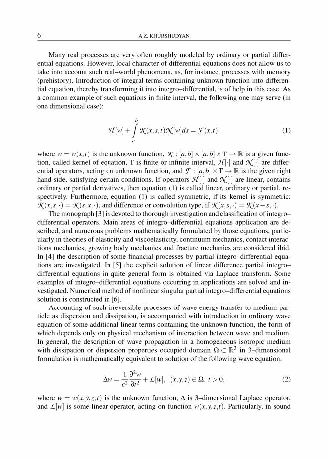
Let us add, that σk = O(k) when k→∞, i.e. for k large enough they became equidis-tant. Moreover, as a result of calculations was observed, that Mpk = O(k−3), p = 1;2,when k→∞, which justifies truncation of infinite system (15), at that they do not dependon factor α in range [0.01,10] for large k. Boundary optimal control function (22) is plot-ted in Fig. 1–2, when n = 80 and a = 0.25; 0.5; 1; 2. From this graphs it is obvious, thatwhen parameter a increases, absolute value of controls also increases.

Figure 1. Optimal control function for n = 80: uo80(t).

As second illustrative example, let us consider L2–optimal solution of system (17)for the second problem, when

φ(t) = cos(t), ψ(t) = sin(2t), w−π(x) = (x−1)cos(πx), w−π =−2xcos(πx),

wπ(x) = (x−1)cos(2πx), wπ = 2xcos(2πx), (x, t) ∈ [0,1]× [−π,π],

and p(x) = δ(x− x0), κ(t) = −b|t|−1, t ∈ [−π,π], b = const ∈ R+. Note, that trans-mission conditions, concerning chosen data are satisfied. Kernel κ(t) in this case alsosatisfies condition a) of Corollary 1. Moreover, κ1(σ) = 2b(γ+ ln |σ|), where γ is Eu-ler‘s constant, and, therefore choosing parameter b in a certain manner one may satisfycondition b) of Corollary 1 as well. Substituting results in (14), we will obtain

zk =βk√

Λ(

β2k · e

1αb+2γ

) , β2k =

(πk)2

αb, k = 1,2,3, ...,


Figure 2. Optimal control function for n = 80: uo80(t).

where Λ(x) is Lambert‘s function [21]. Taking into account properties of that functionone may prove, that all roots zk, k = 1,2,3, ..., in this case are real, i.e. ςk = 0, andzk = O(k) and Mpk = O(k−3), p = 1;2, when k→ ∞ as well, at that they do not dependon factor α in range [0.01,10] for large k. Optimal control function (25) is plotted in Fig.3–6 when n = 80 and x0 = 0.685.

Figure 3. Optimal control function for b = 0.001.

20 A.Z. KHURSHUDYAN



It was discovered that when parameter b increases, absolute value and frequency ofcontrol impacts decrease, and for large values of that parameter coefficients Λo

1k of sines‘in expression (25) dominate coefficients Λo

2k of cosines‘, which is connected with choiceof boundary functions. It was also observed, that absolute value of control function doesnot signally depend on point x0 of control concentration except cases x0→ 0 and x0→ 1mentioned above.


Figure 6. Optimal control function for b = 20.

Note that for chosen parameters of system (8)–(9) the quantities (24) and (26) arealways positive.

7. Conclusions

In the paper solution of control problem of partial integro-differential equation ofconvolution type when control process is realized by boundary functions (the first prob-lem) or right hand side (the second problem) is reduced to minimization procedure ofchosen optimality criterion under constraints of equality type on unknown function andis obtained in explicit form (see (18) and (22) or (25)). According to the main result(Theorem 1) for determination of resolving optimal control is required:

Step 1. To find roots of a characteristic transcendent equation, containing only Fouriertransform of equation kernel (see (12)),

Step 2. Using those roots to separate real and imaginary parts of a system of equalitieswith respect to unknown function Fourier transform (see (11)) and to obtainthe corresponding system of moments problem (see (15)),

Step 3. Applying control formulae for corresponding optimality criterion (see (18) and(22) or (25)), to determine desired function of optimal control,

Step 4. To check if the necessary and sufficient condition of control problem solvabilityis satisfied (see (20) and (24) or (26)).

22 A.Z. KHURSHUDYAN

One of the main aims of this paper concerning efficiency of suggested control al-gorithms from numerical calculations viewpoint, we think, is achieved. As a matter offact, L1–optimal solution determination was reduced to conditional minimum problem,which can be attacked by well–known techniques of variational calculus [19], and L2–optimal solution determination was reduced to solution of a system of linear algebraicequations.

What concerns to criteria considered above, let us note that in fact, the first crite-rion is convenient to set, for instance, when one needs to have an electromagnetic outputpulse, and the second criterion -on the contrary, when one needs to have a continu-ous output signal from discrete input signal. We hope that this method will be appliedwith the same efficiency to control problems investigation for other equations, contain-ing convolution of unknown function, as ordinary as well as partial integro-differentialequations with variable limit of integration.

References

[1] A.G. BUTKOVSKII: Methods of Control of Distributed Parameters Systems. Naukapubl., Moscow, 1975, (in Russian).

[2] V.D. BLONDEL and A. MEGRETSKI (ED): Unsolved Problems in MathematicalSystems and Control Theory. Princeton University Press, Princeton, 2004.

[3] J.M. APPEL, A.S. KALITVIN and P.P. ZABREJKO: Partial Integral Operators andIntegro–Differential Equations. M. Dekkar, New York, 2000.

[4] E.W. SACHS and A.K. STRAUSS: Efficient solution of partial integro–differentialequation in finance. Applied Numerical Math., 58(11) (2008), 1687-1703.

[5] J. THORWE and S. BHALEKAR: Solving partial integro–differential equations usingLaplace transform method. American J. of Computational and Applied Math., 2(3)(2012), 101-104.

[6] J.M. SANZ-SERNA: A numerical method for a partial integro–differential equation.SIAM J. Numerical Analysis, 25(2) (1998), 319-327.

[7] M.B. VINOGRADOVA, O.V. RUDENKO and A.P. SUKHORUKOV: Theory ofWaves, 2nd ed., Nauka publ., Moscow, 1990, (in Russian).

[8] K. BALACHANDRAN and E.R. ANANDHI: Boundary controllability of integrodif-ferential systems in Banach spaces. Proc. of Indian Academy of Sciences, 111(1)(2001), 127-135.

[9] SH. CHIANG: Numerical minimum time control to a class of singular integro–differential equations. Abstracts of MMAAMOE, Tartu, Estonia, (2013).


[10] S. KERBAL and Y. JIANG: General integro–differential equations and optimal con-trols in Banach spaces. J. of Industrial and Management Optimization, 3(1) (2007),119-128.

[11] A.S. SMYSHLYAEV: Explicit and parameter–adaptive boundary control laws forparabolic partial differential equations. PhD thesis, University of California, SanDiego, 2006.

[12] A.ZH. KHURSHUDYAN: On optimal boundary control of non–homogeneous stringvibrations under impulsive concentrated perturbations with delay in controls. Math-ematical Bulletin of T. Shevchenko Scientific Society, 10 (2013), 203-203.

[13] A.ZH. KHURSHUDYAN and SH.KH. ARAKELYAN: Delaying control of non–homogeneous string forced vibrations under mixed boundary conditions. IEEE Pro-ceedings on Control and Communication, 10 (2013), 1-5.

[14] N.N. KRASOVSKII: Motion Control Theory. Nauka publ, Moscow, 1968, (in Rus-sian).

[15] G.E. SHILOV: Mathematical Analysis. The Second Special Course, 2nd ed. MSUpubl., Moscow, 1984, (in Russian).

[16] P. HILLION: Electromagnetic pulse propagation in dispersive media, Progress inElectromagnetics Research, 35 (2002), 299-314.

[17] F.D. GAKHOV and YU.I. CHERSKII: Convolution Type Equations, Nauka publ.Moscow, 1978, (in Russian).

[18] A.F. VORONIN: Necessary and sufficient well–posedness conditions for a convo-lution equation of the second kind with even kernel on a finite interval. SiberianMath. Journal, 48(4) (2008), 601-611.

[19] J.T. BETTS: Practical Methods of Optimal Control Using Nonlinear Programming.SIAM, Advances in Design and Control, 2001.

[20] E.KH. GRIGORYAN and K.L. AGHAYAN: On a new method of asymptotic formu-las determination in waves diffraction problems. Reports of NAS of Armenia, 110(3)(2010), 261-271.

[21] R.M. CORTES, G.H. GONNET, D.E.G. HARE, J.D. JEFFREY and D.E. KNUTH:On the Lambert W function. Advances in Computational Mathematics. 5(1) (1996),329-359.

24 A.Z. KHURSHUDYAN

Appendix

Proof [Proof of Theorem 1]According to method of Cauchy, the fundamental solution of system (10) can be

written as follows:w1(x,σ) = a+eχ(σ)x +a−e−χ(σ)x+

+1

χ(σ)

x∫0

[U1(ξ,σ)+W (ξ,σ)

]sinh[(x−ξ)χ(σ)]dξ, (A1)

(x,σ) ∈ (0,1)×R,

where

a±(σ) =[ψ1(σ)−Φ(σ)]e±χ(σ)−φ1(σ)

e±2χ(σ)−1, χ(σ) = i|σ|

√1+ακ1(σ), (A2)

Φ(σ) =1

χ(σ)

1∫0

[U1(ξ,σ)+W (ξ,σ)

]sinh[(1−ξ)χ(σ)]dξ,

As w1(x, t) is compactly supported function in [−θ,θ] then it is well known [15], that itsFourier generalized transform w1(x,z) is an analytical entire function in whole complexplane z = σ+ iς, satisfying inequality

|zρ ·w1(x,z)|¬ Aρeθ|ς|

for all x ∈ [0,1]; ρ = 0,1,2, ..., and some corresponding constant Aρ 0.In view of W (·, t) is compactly supported in [−θ,θ], one may show that if U1(·, t)

is compactly supported in [−θ,θ] as well, integral term on the right hand side of (A1)extended for all z = σ+ iς is analytic entire function. Therefore, using that extension onemay prove that the function w1(x,z) satisfies recalled theorem conditions if and only ifa± = a±(z) are analytic entire functions. From expressions (A2) extended for all z∈C itis easy to see, that they are entire or not simultaneously. Thus, for example, a+ = a+(z)is an entire analytical function if and only if conditions (11) and (12) are satisfied.

The same reasoning was made in the case of distributed control.When proving Corollary 1, instead of formula (A1) and (A2) the following must be

used:w1(x,σ) = φ1(σ)cos(χ(σ)x)+

+[ψ1(σ)−Φ(σ)]−φ1(σ)cos(χ(σ))

sin(χ(σ))sin(χ(σ)x)+

+1

χ(σ)

x∫0

[U1(ξ,σ)+W (ξ,σ)

]sin[(x−ξ)χ(σ)]dξ, (x,σ) ∈ (0,1)×R,


where

Φ(σ) =1

χ(σ)

1∫0

[U1(ξ,σ)+W (ξ,σ)

]sin[(1−ξ)χ(σ)]dξ,

χ(σ) = |σ|√

1+ακ1(σ)> 0.

The rest part of the proof is similar to proof of Theorem 1.It should be noted, that conditions a) and b) of Corollary 1 have simple physical

treatment. It turns out, that the quantity ε(σ) = 1+ακ1(σ) is complex dielectric per-mittivity of isotropic medium with dispersion property [7, 16], and those conditions areequivalent to assumption, that quantity ε(σ), σ ∈ R, is real–valued, because if so it ispositive for all known materials. On the other hand, with increase of propagating sig-nal frequency to values similar to eigenfrequency of medium, the difference betweendielectric and conducting abilities of medium decreases, and it turns out, that existenceof imaginary part in dielectric permittivity expression from macroscopic point of view isindistinguishable from conducting ability; they both lead to heat evaluation. Thus, bothconditions of Corollary 1 are practically realizable.

If one needs to obtain controlled electromagnetic wave, he has to apply Fourierinverse generalized transform to (A1).

Proof [Proof of Theorem 3]Necessary and sufficient condition (20) is obtained from general existence theorem

for moments problem solution [14]. According to it, for solvability of system (17) it isnecessary and sufficient, that the norm of functions ho

n(t) in space, adjoint to the space ofcontrol function to be finite and non–zero. Since the space L1[−θ,θ] is taken as controlfunction space, and the space adjoint to it is the space of infinite measurable functionsL∞[−θ,θ] with norm ||ho

n||L∞[−θ,θ] = supt∈[−θ,θ] |hon(t)| ≡ [ρo

n]−1, therefore in view of (18)

and (19) we will get (20). Note, that topology in L∞ instead of sup–norm might beintroduced through esssup–norm denoting essential sup of a function [14].

Further, the countable system (15) is resolvable if and only if finite system (17) isresolvable for all n ∈ N [1]. Thus, theorem is proved.

Proof [Proof of Theorem 4]is similar to proof of Theorem 3, but in this case in view of selfadjointness of space

L2[−θ,θ] we have ρon =

[||uo

n(t)||L2[−θ,θ]]−2.

On Optimal Boundary and Distributed Control of Partial Integro-Differential Equations. Об...

Documents

Transcript of On Optimal Boundary and Distributed Control of Partial Integro-Differential Equations. Об...