Digital Object Identifier (DOI) 10.1007/s00211-004-0530-0Numer. Math. (2004) Numerische

Mathematik

Convergence of numerical schemes for viscositysolutions to integro-differential degenerate parabolicproblems arising in financial theory

Maya Briani1, Claudia La Chioma2, Roberto Natalini3

1 Universita di Roma “La Sapienza”, Dipartimento per le Decisioni Economiche e Finan-ziarie, Via del Castro Laurenziano, 00161 Roma, Italy; e-mail: m.briani@iac.cnr.it

2 Universita di Roma “La Sapienza”, Dipartimento di Matematica Pura ed Applicata,Piazzale Aldo Moro, 2, 00161 Roma, Italy; e-mail: c.lachioma@iac.cnr.it

3 Istituto per le Applicazioni del Calcolo “Mauro Picone”, Consiglio Nazionale delleRicerche, Viale del Policlinico, 137, 00161 Roma, Italy; e-mail: r.natalini@iac.cnr.it

Received March 25, 2002 / Revised version received February 13, 2003 /Published online August 6, 2004 – c© Springer-Verlag 2004

Summary. We study the numerical approximation of viscosity solutions forintegro-differential, possibly degenerate, parabolic problems. Similar modelsarise in option pricing, to generalize the celebrated Black–Scholes equation,when the processes which generate the underlying stock returns may con-tain both a continuous part and jumps. Convergence is proven for monotoneschemes and numerical tests are presented and discussed.

Mathematics Subject Classification (1991): 65M12, 35K55, 49L25

1. Introduction

In this paper we study the numerical approximation of a class of semilinearstrongly degenerate parabolic integro-differential Cauchy problems of thefollowing form:

{∂tu− LI(x, t, I,D,D2)u+H(x, t,Du, Iu) = 0,

u(x, 0) = u0(x),(1.1)

where u0 is a continuous initial data, LI is a linear degenerate elliptic opera-tor andH is a nonlinear first order operator. Here Iu is an integral term givenby

Correspondence to: R. Natalini

M. Briani et al.

Iu =∫

RD

M(u(x + z, t), u(x, t))µx,t (dz),(1.2)

where µx,t is a positive bounded measure and M is a function which is nondecreasing in the first argument, M(u, u) = 0 and such that

M(u, v)−M(w, z) ≤ c((u− w)+ + |v − z|).Problems in this form arise when considering a financial derivative con-structed on an underlying asset given, as in Merton [31], by a jump-diffusionprocess instead of the classical diffusion dynamics, in order to have a morerealistic description of the market than the one obtained with the Black–Scho-les model [11]. In particular, using the original Black–Scholes formula, theimplied volatilities vary for different strikes and maturities, producing theso–called volatility skew or smile. On the contrary, a suitable choice of thejump process parameters can allow the model to fit the observed volatility.For some recent works concerning jump-diffusion models see [1,7,10,20,27]. Another recent domain of interest is the analytical modeling of jumpsin fixed-income markets, [8,13,14,17,18,20,33]. The choice of a jump dif-fusion model in this setting seems to be the natural one [25,18]; it is worthnoticing that this choice preserves the mean reverting behaviour of the inter-est rate curve. More direct numerical issues are considered in [6] and in thebook by D. Tavella and C. Randall [35].

From a mathematical perspective, the problem of existence and unique-ness of solutions to these equations has been intensively studied in the frame-work of classical solutions and for uniformly parabolic operators, see [21–23]and references therein. Unfortunately, due to the possible degeneracy of theparabolic operator, typical of incomplete markets [30,3,4], and the pres-ence of nonlinear terms, as for instance in Example 2.2, we have to considerweaker (not continuously differentiable) solutions. This last is not a mathe-matical complication, as the typical example of nonlinearity is given by thelarge investor model, in which the movements of big amounts of money by asingle investor influence the market itself, in particular the interest rate. More-over it is worth noticing that in the real world banks apply different rates forborrowing or lending and this also brings nonlinear effects in the model. Anatural approach is given by viscosity solutions [15]. In this framework, theintegro-differential problems have been first studied by Alvarez and Tourin[2]. In particular they studied the equation

∂tu+ F(x, t, u,Du,D2u) = Iu,where F is a pure differential second order elliptic operator, F ∈ C(RD ×(0, T ]×R×R

D×SD), and Iu is defined as above. We follow their approach,using an extended notion of viscosity solutions and viscosity inequalities,considering that the classical theory of [15] was simply concerned with the

Convergence of numerical schemes arising in financial theory

purely differential case. More general results and problems can be found in[3–5] and references therein.

A great deal has been done for the numerical approximation of viscositysolutions, starting from [16]. For second order problems let us refer to thefundamental paper by Barles and Souganidis [9], who first showed conver-gence results for a large class of numerical schemes to the solution of fullynonlinear second order elliptic or parabolic PDE. Following their tracks, wehere extend their arguments to the class of numerical schemes for integro-differential problems.

Let us also recall that in the framework of linear problems with constantcoefficients, this new integral term was already considered in [6]. In that paperthe authors proposed to use an operator splitting method compared with thedrawbacks of a pure Crank-Nicholson one. In that context, the method wasshown to be quite effective: it had a lighter computational burden and allowedto couple the differential part, with an implicit finite difference method, andthe integral part, with an FFT method. The FFT method requires a constantgrid step, however it could diminish the numerical precision of the schemein some areas; it is possible to overcome this difficulty using an asymptoticprofile of the solution or a particular feature of the integral operator. A closerdiscussion of this method is done in Section 7. We here wish to underlinethat its rigorous assessing, as well as its extension to fully nonlinear stronglydegenerate problems, which are the main objectives of our investigation,seems to be quite difficult and still has to be done.

Another difficult problem stems from the integral term. It is necessary totruncate the problem domain on one hand, and the integral domain on theother. As µx,t is a bounded measure, for a fixed ν > 0 we can choose abounded computational domain Dν for the integral term, such that

∣∣∣∫

RD

µx,t (dz)−∫Dν

µx,t (dz)

∣∣∣ < ν,

and we can consider a new problem with Iνu = ∫DνM(u(x + z, t),

u(x, t))µx,t (dz) instead of Iu; after that, we have to truncate the domainof the problem.

Unfortunately, due to the non-local nature of the integral term, once wehave found a given domain, we still need to use some approximation of thesolution in a larger computational domain. The common approach consistsin replacing the original problem with an homogeneous one, i.e. withoutthe integral term, or to use some asymptotic representation formula for thesolution.

Here we try a different approach. First we show that our original problemcan be well approximated by a pure differential problem with an artificial dif-fusion. We apply this remark to implement an effective numerical boundary

M. Briani et al.

condition, giving as a consequence a full convergence result for the globalapproximation scheme.

The article is organized as follows: in Section 2 we briefly describe thebasic financial models, and in particular we introduce some details of the non-linear model for a large investor; in Section 3 we recall some basic definitionsand results concerning viscosity solutions, while the main convergence resultis given in Section 4; Section 5 is devoted to the study of the numerical compu-tation of the integral term and the study of the scheme in the one dimensionalcase; in Section 6 we show that we can approximate the integro–differentialoperator by a suitable diffusive differential model. In Section 7 we focus onnumerical simulations: after a short review of some recent numerical meth-ods for the linear PIDE, we give a quite complete description of our explicitscheme. In particular Subsection 7.2 deals with the numerical boundary con-ditions and proves that, under proper assumptions on the measure µx,t andon the grid steps, the whole scheme is second order accurate.

We conclude, in Section 8, by presenting some numerical examples. Firstwe deal with the classical Morton equation. A two dimensional problem isstudied in Subsection 8.2. In Subsection 8.3, we consider the large investornonlinear case.

2. The financial model - option pricing with jump-diffusion processes

For the basic notions on financial markets we refer to [12]. Following theseminal paper by Merton [31], we consider models which take into accountabrupt price movements caused by exogenous events or information. The aimis to avoid the discrepancies between the results given by the standard Black–Scholes model [11] and empirical evidence. For instance it is well-known thatthe implied volatility, fitted by using historical data in the Black–Scholes for-mula, is not a constant, but depends on the strike price and on the expirationtime. Actually, in addition to small variations from the trend, which maybe described by a Brownian motion, the analysis of price evolution revealssudden and rare breaks. Therefore, from a probabilistic point of view, it isnatural to model such behavior by some point processes that count the occur-rences of rare and random events. We then consider a market whose moneymarket account evolves according to the differential equation

dS0t = S0

t rdt,

where r stands for a deterministic interest rate, while S = (S1, ..., SD), therisky assets, are described by a stochastic differential system of jump-diffu-sion type:

dSit = Sit−[µidt +

P∑j=1

σijdWjt +

M∑k=1

γikdNkt

], i = 1, ..., D.

Convergence of numerical schemes arising in financial theory

Here Wt = (W 1t , ...,W

Pt ) is a P -dimensional Brownian motion, Nt =

(N1t , ..., N

Mt ) is a M-dimensional Poisson process.

Remark 2.1. If all the γik are zero, and the functions µ and σ are constant,we have the standard Black–Scholes model, where the stock price follows alog-normal random walk:

dSt = St(µdt + σdWt).

It is well known that Black and Scholes assumed ideal conditions inthe market: there are no arbitrage opportunities and the market is complete.Constructing directly the hedging strategy, that is given deterministically as afunction of (St , t), we get the arbitrage price of the European contingent claim(T ,G) as the solution of the linear final value problem on (0,+∞)× (0, T ):

−∂tV = 1

2σ 2S2∂2

SSV + r∂SSV − rV ,

V (S, T ) = G(S).

(2.1)

Example 2.1. [Merton model] The prototype of jump-diffusion market hasbeen first proposed by Merton [31]. The underlying process’ dynamics aregiven by the following equation:

dSt

St= (µ− λk)dt + σdWt + (η − 1)dNt .

where dWt is a standard Brownian motion, dNt is a Poisson counting processof intensity λ, that is:

dNt =

0 with probability 1 − λdt

1 with probability λdt.

Moreover we are assuming that η is a log-normally distributed jump ampli-tude with probability density:

�δ(η) = exp(− 12 (

log ηδ)2)√

2πδη,(2.2)

k is the expectation E(η−1), and the Brownian and the Poisson processes are

uncorrelated. Setting J V (S) = λ( ∫

D

V (Sη)�δ(η)dη − V)

, we promptly

obtain by the Ito formula the following pricing equation

∂V

∂t+ 1

2σ 2S2 ∂

2V

∂S2+ (r − λk)S

∂V

∂S− rV + J V

= ∂V

∂t+ LJ V = 0,(2.3)

M. Briani et al.

with D = [0,+∞) and the final condition

V (T , ST ) = VT (ST ).

Following [3,4,36], it is possible to consider more sophisticated models,namely the large investor economy: let ξ(V,DV,J V ) = V −Sσθ0 ·DV −φ0 ·J V denote the amount of money invested in stocks by the agent, obtainedchoosing a proper replicating portfolio; then the interest rate r is influencedby the agents by means of ξ . Usually r is a non-increasing function of ξ , butwe shall suppose that r(·, ξ)ξ is non decreasing with respect to ξ . In addition,we do not impose that r is continuous with respect to ξ at zero, in order toinclude interesting examples. For details about the parameters θ0 and φ0 werefer to [3].

In this setting the function V must solve the following quasi-linear finalvalue problem:

∂tV + LJ V = H(S, t, V ,J V,DV ),

V (S, T ) = G(S),

(2.4)

where we have simply rewritten equation (2.3) with the addition of the non-linear first order operator:

H(S, t, V ,J V,DV ) = r(S, t, ξ) · ξ.(2.5)

Obviously, if all the parameters of the model r , µi , σij and γij are determin-istic function of (S, t), the problem is linear and we obtain the so called smallinvestor economy.

Example 2.2. [Completion of the market in the large investor model] It is eas-ily proven that a jump-diffusion market is incomplete because of the arbitrageopportunities arising at the jump time (see [12]). To overcome the difficultyof pricing a derivative it is possible to complete the jump-diffusion market byadding another derivative on the same underlying asset. A standard approachis to add a call whose parameters are taken directly from the market, and notby Ito rule. Therefore we can suppose that our market is described by

dS0

t = S0t r(X, t, ξ)dt,

dX = Xαdt + XβdWt + X(γ − 1)dWt,

+Xt (γ 1)dNt

where Xt = diag(St , Ct ) and the vectors of expectation α, volatility β, andjump γ are:

α =(µ− λk

µC

), β =

(σ

σC

), γ =

(η

ηC

).

Convergence of numerical schemes arising in financial theory

The jump amplitude γ is now lognormally distributed with density

�(γ ) = �(η) · �C(ηC).

In this frameset the pricing equation is the extension of (2.3) to the multidi-mensional case:

∂tV + LJ V = H(S, t, V ,J V,DV ),

V (X, T ) = G(X).

Here, the operator

LJ V = 1

2tr[(Xβ)(Xβ)TD2V ] + X[α + βθ ] · DV − φ · J V,

is linearly degenerate elliptic. MoreoverH has the same form as (2.5), withXplaying the role of S, and J V as previously withD = [0,+∞)× [0,+∞).We can note that in this case the diffusion matrix is degenerate, since

rk((Xβ)(Xβ)T ) < 2.

If we apply a change of variable in order to have diffusion only in one direc-tion: (

x

y

)=

(cosϑ sin ϑ

− sin ϑ cosϑ

)·(

log SlogC

),

with ϑ = arctg σCσ

, and proper coefficients A, B, C, D we obtain:

∂tu+ 1

2(σ 2 + σ 2

C)∂2xxu+ A∂xu+ B∂yu− φIu

= r(x, y, t, u+ C∂xu+D∂yu− φ0Iu

)

×(u+ C∂xu+D∂yu− φ0Iu

),(2.6)

where:

Iu = λ( ∫ +∞

−∞

∫ +∞

−∞u(x + ξ, y + ζ, t)

exp (− ξ2+ζ 2

2δ2 )

2πδρ

· exp(

− (δ2 − ρ2)(ξ sin θ + ζ cos θ)2

2δ2ρ2

)dξdζ − u(x, y, t)

).

This example shows the need for a theory of strongly degenerate nonlinearparabolic operators in financial applications.

M. Briani et al.

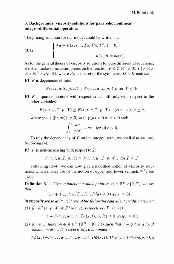
3. Backgrounds: viscosity solutions for parabolic nonlinearintegro-differential operators

The pricing equation for our model could be written as:∂tu+ F(x, t, u, Iu,Du,D2u) = 0,

u(x, 0) = u0(x),

(3.1)

As for the general theory of viscosity solutions for pure differential equations,we shall make some assumptions on the function F ∈ C(RD × [0, T ] × R ×R × R

D × SD,R), where SD is the set of the symmetric D ×D matrices.

F1 F is degenerate elliptic:

F(x, t, u, I, p,X ) ≥ F(x, t, u, I, p,Y), for X ≤ Y;F2 F is quasi-monotone with respect to u, uniformly with respect to the

other variables:

F(x, t, u, I, p,X ) ≥ F(x, t, v, I, p,X )− γ (u− v), u ≥ v,

where γ ∈ C([0,∞)), γ (0) = 0, γ (u) > 0 as u > 0 and:∫ ε

0

du

γ (u)= ∞ for all ε > 0.

To rely the dependency of F on the integral term, we shall also assume,following [4],

F3 F is non-increasing with respect to I:

F(x, t, u, I, p,X ) ≥ F(x, t, u,J , p,X ), for I ≤ J .Following [2–4], we can now give a modified notion of viscosity solu-

tions, which makes use of the notion of upper and lower semijets P±, see[15].

Definition 3.1. Given a function u and a point (x, t) ∈ RD × [0, T ), we say

that:∂tu+ F(x, t, u, Iu,Du,D2u) ≤ 0 (resp. ≥ 0)

in viscosity sense at (x, t) if one of the following equivalent condition is met:

(1) for all (τ, p,X ) ∈ P+u(x, t) (respectively P−(x, t)):

τ + F(x, t, u(x, t), Iu(x, t), p,X ) ≤ 0 (resp. ≥ 0);(2) for each function φ ∈ C2,1(RD × [0, T )) such that u − φ has a local

maximum at (x, t) (respectively, a minimum):

∂tφ(x, t)+F(x, t, u(x, t), Iφ(x, t),Dφ(x, t),D2φ(x, t))≤0 (resp.≥0);

Convergence of numerical schemes arising in financial theory

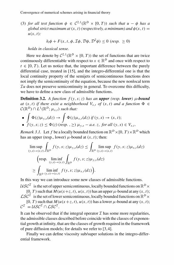
(3) for all test function φ ∈ C2,1(RD × [0, T )) such that u − φ has aglobal strict maximum at (x, t) (respectively, a minimum) and φ(x, t) =u(x, t):

∂tφ + F(x, t, φ, Iφ,Dφ,D2φ) ≤ 0 (resp. ≥ 0)

holds in classical sense.

Here we denote by C2,1(RD × [0, T )) the set of functions that are twicecontinuously differentiable with respect to x ∈ R

D and once with respect tot ∈ [0, T ). Let us notice that, the important difference between the purelydifferential case, treated in [15], and the integro-differential one is that thelocal continuity property of the semijets of semicontinuous functions doesnot imply the semicontinuity of the equation, because the new nonlocal termIu does not preserve semicontinuity in general. To overcome this difficulty,we have to define a new class of admissible functions.

Definition 3.2. A function f (y, s; z) has an upper (resp. lower) µ-boundat (x, t) if there exist a neighborhood Vx,t of (x, t) and a function � ∈C(RD) ∩ L1(RD;µx,t ) such that:

•∫�(z)µy,s(dz) →

∫�(z)µx,t (dz) if (y, s) → (x, t);

• f (y, s; z) ≤ �(z) (resp. ,≥) µy,s − a.e. z, for all (y, s) ∈ Vx,t .Remark 3.1. Let f be a locally bounded function on R

D×[0, T )×RD which

has an upper (resp., lower) µ-bound at (x, t); then:

lim sup(y,s)→(x,t)

∫RD

f (y, s; z)µy,s(dz) ≤∫

RD

lim sup(y,s)→(x,t)

f (y, s; z)µx,t (dz)(

resp. lim inf(y,s)→(x,t)

∫RD

f (y, s; z)µy,s(dz)

≥∫

RD

lim inf(y,s)→(x,t)

f (y, s; z)µx,t (dz)).

In this way we can introduce some new classes of admissible functions.

USCI is the set of upper semicontinuous, locally bounded functions on RD×

[0, T ) such thatM(u(x+z, t), u(x, t))has an upperµ-bound at any (x, t);LSCI is the set of lower semicontinuous, locally bounded functions on R

D×[0, T ) such thatM(u(x+z, t), u(x, t)) has a lowerµ-bound at any (x, t);

CI = USCI ∩ LSCI .

It can be observed that if the integral operator I has some more regularities,the admissible classes described before coincide with the classes of exponen-tial growth at infinity, that are the classes of growth required in the frameworkof pure diffusion models; for details we refer to [3,4].

Finally we can define viscosity sub/super solutions in the integro-differ-ential framework.

M. Briani et al.

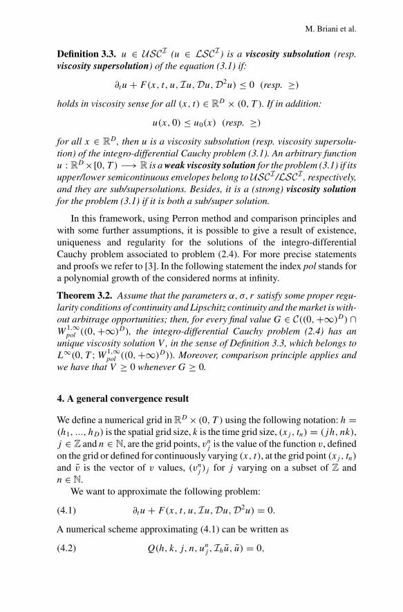
Definition 3.3. u ∈ USCI (u ∈ LSCI) is a viscosity subsolution (resp.viscosity supersolution) of the equation (3.1) if:

∂tu+ F(x, t, u, Iu,Du,D2u) ≤ 0 (resp. ≥)holds in viscosity sense for all (x, t) ∈ R

D × (0, T ). If in addition:

u(x, 0) ≤ u0(x) (resp. ≥)for all x ∈ R

D, then u is a viscosity subsolution (resp. viscosity supersolu-tion) of the integro-differential Cauchy problem (3.1). An arbitrary functionu : R

D×[0, T ) −→ R is a weak viscosity solution for the problem (3.1) if itsupper/lower semicontinuous envelopes belong to USCI /LSCI , respectively,and they are sub/supersolutions. Besides, it is a (strong) viscosity solutionfor the problem (3.1) if it is both a sub/super solution.

In this framework, using Perron method and comparison principles andwith some further assumptions, it is possible to give a result of existence,uniqueness and regularity for the solutions of the integro-differentialCauchy problem associated to problem (2.4). For more precise statementsand proofs we refer to [3]. In the following statement the index pol stands fora polynomial growth of the considered norms at infinity.

Theorem 3.2. Assume that the parameters α, σ, r satisfy some proper regu-larity conditions of continuity and Lipschitz continuity and the market is with-out arbitrage opportunities; then, for every final value G ∈ C((0,+∞)D) ∩W

1,∞pol ((0,+∞)D), the integro-differential Cauchy problem (2.4) has an

unique viscosity solution V , in the sense of Definition 3.3, which belongs toL∞(0, T ;W 1,∞

pol ((0,+∞)D)). Moreover, comparison principle applies andwe have that V ≥ 0 whenever G ≥ 0.

4. A general convergence result

We define a numerical grid in RD × (0, T ) using the following notation: h =

(h1, ..., hD) is the spatial grid size, k is the time grid size, (xj , tn) = (jh, nk),j ∈ Z and n ∈ N, are the grid points, vnj is the value of the function v, definedon the grid or defined for continuously varying (x, t), at the grid point (xj , tn)and v is the vector of v values, (vnj )j for j varying on a subset of Z andn ∈ N.

We want to approximate the following problem:

∂tu+ F(x, t, u, Iu,Du,D2u) = 0.(4.1)

A numerical scheme approximating (4.1) can be written as

Q(h, k, j, n, unj , Ihu, u) = 0,(4.2)

Convergence of numerical schemes arising in financial theory

where Ihu denotes the integral approximation. We want to prove that, undersuitable conditions, this scheme converges to the solution of the problem(4.1), provided that this problem satisfies proper conditions.

Properties of the scheme

H1 Monotonicity of the approximating integral.If u ≥ v and unj = vnj we have the following inequality:

Ihu ≥ Ihv;(4.3)

H2 Stability.

For all h, k a solution u does exist that is bounded

independently from (h, k);(4.4)

H3 Consistency.For all φ ∈ C∞

b (RD × [0, T ]) and for all (x, t) ∈ R

D × (0, T ) we have:

lim inf(h,k)→0

(jh,nk)→(x,t)

ξ→0

Q(h, k, j, n, φnj + ξ, Ih(φ + ξ), φ + ξ)

ρ(h, k)

≥ ∂tu+ F(x, t, u, Iu,Du,D2u);(4.5)

lim sup(h,k)→0

(jh,nk)→(t,x)

ξ→0

Q(h, k, j, n, φnj + ξ, Ih(φ + ξ), φ + ξ)

ρ(h, k)

≤ ∂tu+ F(x, t, u, Iu,Du,D2u);(4.6)

H4 Monotonicity.If u ≥ v and unj = vnj for all h, k ≥ 0 and 1 ≤ n ≤ N , we have:

Q(h, k, n, j, unj , Ihu, u) ≤ Q(h, k, n, j, vnj , Ihv, v).(4.7)

Remark 4.1. The theory of numerical approximation of fully nonlinear degen-erate parabolic problems [9] could be considered as a special case of thepresent one. We define the numerical scheme approximating the parabolicproblem:

∂tu+ F(x, t, u, 0,Du,D2u) = 0 in RD × (0, T ),(4.8)

M. Briani et al.

as:

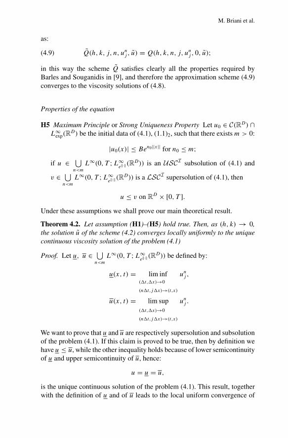
Q(h, k, j, n, unj , u) = Q(h, k, n, j, unj , 0, u);(4.9)

in this way the scheme Q satisfies clearly all the properties required byBarles and Souganidis in [9], and therefore the approximation scheme (4.9)converges to the viscosity solutions of (4.8).

Properties of the equation

H5 Maximum Principle or Strong Uniqueness Property Let u0 ∈ C(RD) ∩L∞

exp(RD) be the initial data of (4.1), (1.1)2, such that there existsm > 0:

|u0(x)| ≤ Ben0||x|| for n0 ≤ m;if u ∈ ⋃

n<m

L∞(0, T ;L∞e‖·‖(R

D)) is an USCI subsolution of (4.1) and

v ∈ ⋃n<m

L∞(0, T ;L∞e‖·‖(R

D)) is a LSCI supersolution of (4.1), then

u ≤ v on RD × [0, T ].

Under these assumptions we shall prove our main theoretical result.

Theorem 4.2. Let assumption (H1)–(H5) hold true. Then, as (h, k) → 0,the solution u of the scheme (4.2) converges locally uniformly to the uniquecontinuous viscosity solution of the problem (4.1)

Proof. Let u, u ∈ ⋃n<m

L∞(0, T ;L∞e‖·‖(R

D)) be defined by:

u(x, t) = lim inf(�t,�x)→0

(n�t,j�x)→(t,x)

unj ,

u(x, t) = lim sup(�t,�x)→0

(n�t,j�x)→(t,x)

unj .

We want to prove that u and u are respectively supersolution and subsolutionof the problem (4.1). If this claim is proved to be true, then by definition wehave u ≤ u, while the other inequality holds because of lower semicontinuityof u and upper semicontinuity of u, hence:

u = u = u,

is the unique continuous solution of the problem (4.1). This result, togetherwith the definition of u and of u leads to the local uniform convergence of

Convergence of numerical schemes arising in financial theory

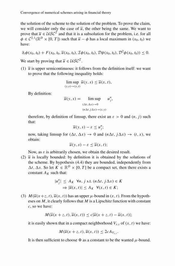
the solution of the scheme to the solution of the problem. To prove the claim,we will consider only the case of u, the other being the same. We want toprove that u ∈ USCI and that it is a subsolution for the problem, i.e. for allφ ∈ C2,1(RD × [0, T ]) such that u − φ has a local maximum in (x0, t0) wehave:

∂tφ(x0, t0)+ F(x0, t0, u(x0, t0), Iφ(x0, t0),Dφ(x0, t0),D2φ(x0, t0)) ≤ 0.

We start by proving that u ∈ USCI .

(1) u is upper semicontinuous: it follows from the definition itself: we wantto prove that the following inequality holds:

lim sup(y,s)→(x,t)

u(y, s) ≤ u(x, t),

By definition:u(y, s) = lim sup

(�t,�x)→0

(n�t,j�x)→(s,y)

unj ,

therefore, by definition of limsup, there exist an ε > 0 and (n, j) suchthat:

u(y, s)− ε ≤ unj ;now, taking limsup for (�t,�x) → 0 and (n�t, j�x) → (t, x), weobtain:

u(y, s)− ε ≤ u(x, t);Now, as ε is arbitrarily chosen, we obtain the desired result.

(2) u is locally bounded: by definition it is obtained by the solutions ofthe scheme. By hypothesis (4.4) they are bounded, independently from�t,�x. So let K ∈ R

D × [0, T ] be a compact set, then there exists aconstant AK such that:

|unj | ≤ AK ∀n, j s.t. (n�t, j�x) ∈ K⇒ |u(x, t)| ≤ AK ∀(x, t) ∈ K;

(3) M(u(x+z, t), u(x, t)) has an upperµ-bound in (x, t). From the hypoth-eses onM , it clearly follows thatM is a Lipschitz function with constantc, so we have:

M(u(x + z, t), u(x, t)) ≤ c|u(x + z, t)− u(x, t)|;it is easily shown that in a compact neighborhood Vx,t of (x, t) we have:

M(u(x + z, t), u(x, t)) ≤ 2cAVx,t .

It is then sufficient to choose� as a constant to be the wanted µ-bound.

M. Briani et al.

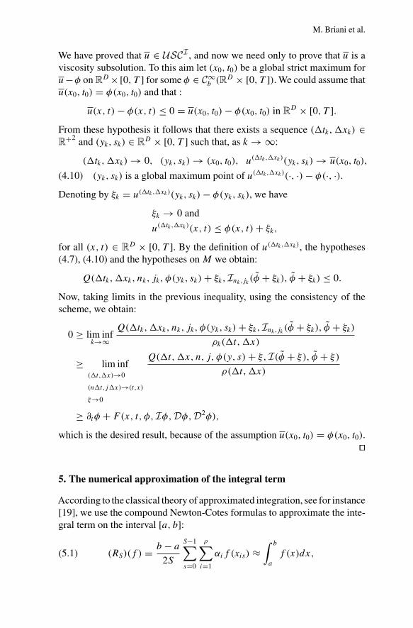
We have proved that u ∈ USCI , and now we need only to prove that u is aviscosity subsolution. To this aim let (x0, t0) be a global strict maximum foru−φ on R

D× [0, T ] for some φ ∈ C∞b (R

D × [0, T ]). We could assume thatu(x0, t0) = φ(x0, t0) and that :

u(x, t)− φ(x, t) ≤ 0 = u(x0, t0)− φ(x0, t0) in RD × [0, T ].

From these hypothesis it follows that there exists a sequence (�tk,�xk) ∈R

+2 and (yk, sk) ∈ RD × [0, T ] such that, as k → ∞:

(�tk,�xk) → 0, (yk, sk) → (x0, t0), u(�tk,�xk)(yk, sk) → u(x0, t0),

(yk, sk) is a global maximum point of u(�tk,�xk)(·, ·)− φ(·, ·).(4.10)

Denoting by ξk = u(�tk,�xk)(yk, sk)− φ(yk, sk), we have

ξk → 0 and

u(�tk,�xk)(x, t) ≤ φ(x, t)+ ξk,

for all (x, t) ∈ RD × [0, T ]. By the definition of u(�tk,�xk), the hypotheses

(4.7), (4.10) and the hypotheses on M we obtain:

Q(�tk,�xk, nk, jk, φ(yk, sk)+ ξk, Ink,jk (φ + ξk), φ + ξk) ≤ 0.

Now, taking limits in the previous inequality, using the consistency of thescheme, we obtain:

0 ≥ lim infk→∞

Q(�tk,�xk, nk, jk, φ(yk, sk)+ ξk, Ink,jk (φ + ξk), φ + ξk)

ρk(�t,�x)

≥ lim inf(�t,�x)→0

(n�t,j�x)→(t,x)

ξ→0

Q(�t,�x, n, j, φ(y, s)+ ξ, I(φ + ξ), φ + ξ)

ρ(�t,�x)

≥ ∂tφ + F(x, t, φ, Iφ,Dφ,D2φ),

which is the desired result, because of the assumption u(x0, t0) = φ(x0, t0).��

5. The numerical approximation of the integral term

According to the classical theory of approximated integration, see for instance[19], we use the compound Newton-Cotes formulas to approximate the inte-gral term on the interval [a, b]:

(RS)(f ) = b − a

2S

S−1∑s=0

ρ∑i=1

αif (xis) ≈∫ b

a

f (x)dx,(5.1)

Convergence of numerical schemes arising in financial theory

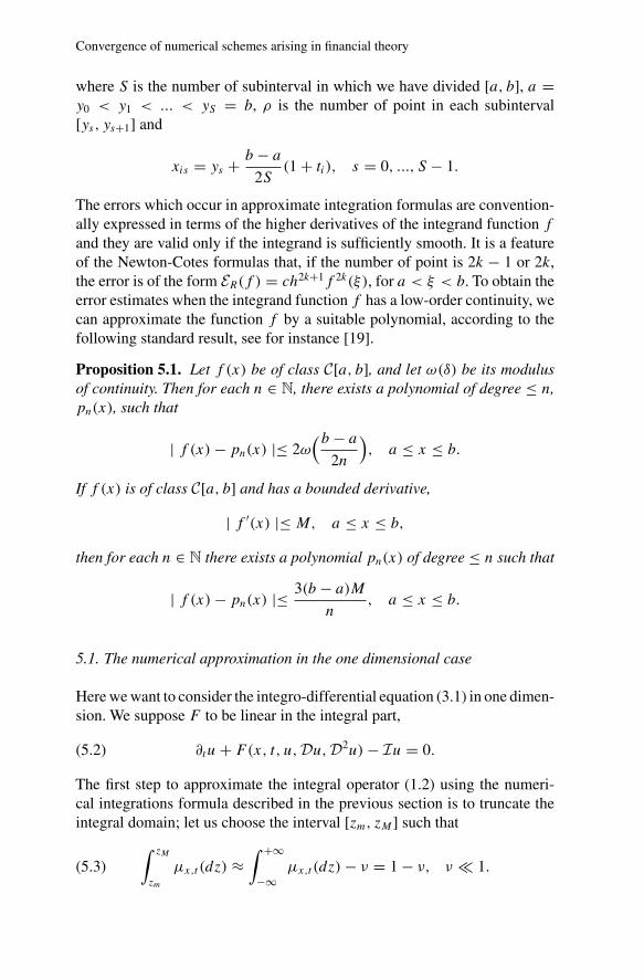
where S is the number of subinterval in which we have divided [a, b], a =y0 < y1 < ... < yS = b, ρ is the number of point in each subinterval[ys, ys+1] and

xis = ys + b − a

2S(1 + ti), s = 0, ..., S − 1.

The errors which occur in approximate integration formulas are convention-ally expressed in terms of the higher derivatives of the integrand function fand they are valid only if the integrand is sufficiently smooth. It is a featureof the Newton-Cotes formulas that, if the number of point is 2k − 1 or 2k,the error is of the form ER(f ) = ch2k+1f 2k(ξ), for a < ξ < b. To obtain theerror estimates when the integrand function f has a low-order continuity, wecan approximate the function f by a suitable polynomial, according to thefollowing standard result, see for instance [19].

Proposition 5.1. Let f (x) be of class C[a, b], and let ω(δ) be its modulusof continuity. Then for each n ∈ N, there exists a polynomial of degree ≤ n,pn(x), such that

| f (x)− pn(x) |≤ 2ω(b − a

2n

), a ≤ x ≤ b.

If f (x) is of class C[a, b] and has a bounded derivative,

| f ′(x) |≤ M, a ≤ x ≤ b,

then for each n ∈ N there exists a polynomial pn(x) of degree ≤ n such that

| f (x)− pn(x) |≤ 3(b − a)M

n, a ≤ x ≤ b.

5.1. The numerical approximation in the one dimensional case

Here we want to consider the integro-differential equation (3.1) in one dimen-sion. We suppose F to be linear in the integral part,

∂tu+ F(x, t, u,Du,D2u)− Iu = 0.(5.2)

The first step to approximate the integral operator (1.2) using the numeri-cal integrations formula described in the previous section is to truncate theintegral domain; let us choose the interval [zm, zM ] such that

∫ zM

zm

µx,t (dz) ≈∫ +∞

−∞µx,t (dz)− ν = 1 − ν, ν � 1.(5.3)

M. Briani et al.

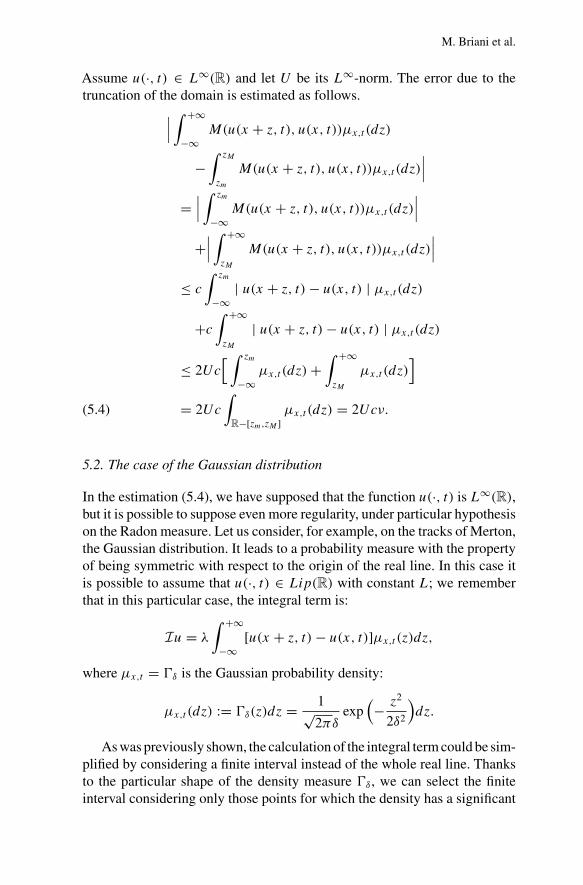
Assume u(·, t) ∈ L∞(R) and let U be its L∞-norm. The error due to thetruncation of the domain is estimated as follows.

∣∣∣∫ +∞

−∞M(u(x + z, t), u(x, t))µx,t (dz)

−∫ zM

zm

M(u(x + z, t), u(x, t))µx,t (dz)

∣∣∣=

∣∣∣∫ zm

−∞M(u(x + z, t), u(x, t))µx,t (dz)

∣∣∣+

∣∣∣∫ +∞

zM

M(u(x + z, t), u(x, t))µx,t (dz)

∣∣∣≤ c

∫ zm

−∞| u(x + z, t)− u(x, t) | µx,t (dz)

+c∫ +∞

zM

| u(x + z, t)− u(x, t) | µx,t (dz)

≤ 2Uc[ ∫ zm

−∞µx,t (dz)+

∫ +∞

zM

µx,t (dz)]

= 2Uc∫

R−[zm,zM ]µx,t (dz) = 2Ucν.(5.4)

5.2. The case of the Gaussian distribution

In the estimation (5.4), we have supposed that the function u(·, t) is L∞(R),but it is possible to suppose even more regularity, under particular hypothesison the Radon measure. Let us consider, for example, on the tracks of Merton,the Gaussian distribution. It leads to a probability measure with the propertyof being symmetric with respect to the origin of the real line. In this case itis possible to assume that u(·, t) ∈ Lip(R) with constant L; we rememberthat in this particular case, the integral term is:

Iu = λ

∫ +∞

−∞[u(x + z, t)− u(x, t)]µx,t (z)dz,

where µx,t = �δ is the Gaussian probability density:

µx,t (dz) := �δ(z)dz = 1√2πδ

exp(− z2

2δ2

)dz.

As was previously shown, the calculation of the integral term could be sim-plified by considering a finite interval instead of the whole real line. Thanksto the particular shape of the density measure �δ, we can select the finiteinterval considering only those points for which the density has a significant

Convergence of numerical schemes arising in financial theory

value and this choice would not introduce big errors. Choose a parameterε > 0 and select the interval [zm, zM ] as the set of all the points z that verify:

�δ(z) ≥ ε ⇐⇒ 1√2πδ

e− z2

2δ2 ≥ ε;

by simple calculation we can derive zm and zM :

−√

−2δ2 log(εδ√

2π) ≤ z ≤√

−2δ2 log(εδ√

2π).

As �δ is a symmetric function with respect to its axis (that in this case is theline z = 0), we define:

zM =√

−2δ2 log(εδ√

2π), zm = −zM.Under these hypotheses we have the following estimate:∣∣∣

∫ +∞

−∞M(u(x + z, t), u(x, t))�δ(dz)

−∫ zM

zm

M(u(x + z, t), u(z, t))�δ(dz)

∣∣∣≤ L

(∫ zm

−∞|z|�δ(dz)+

∫ +∞

zM

|z|�δ(dz)),

therefore∫ zm

−∞|z|�δ(dz)+

∫ +∞

zM

|z|�δ(dz)

= 2∫ +∞

zM

z1√2πδ

exp(− z2

2δ2

)dz = 2δ2

√2π

exp(

− z2M

2δ

)= 2δ2ε.(5.5)

Let us now apply the compound rule (5.1) to the truncated integral.

Ihu = λ(RS)(M�δ) = λzM − zm

2S

S−1∑s=0

ρ∑i=0

αi

×M(u(x + zis, t), u(x, t))�δ(zis).(5.6)

Since the function g(z) = M(u(x + z, t), u(x, t))�δ(z) has a low-ordercontinuity, to get an error estimate for the approximation (5.6), we applyProposition 5.1. Recall that for a generic function f we have

ER(f ) =∫ b

a

f (x)dx − R(f ) =∫ b

a

(f (x)− pn(x))dx

+∫ b

a

pn(x)dx − R(f )

=∫ b

a

(f (x)− pn(x))dx + R(pn − f ).

M. Briani et al.

Then

| ER(f ) |≤((b − a)+

ρ∑i=0

| αi |)

| f (x)− pn(x) | .

If αi > 0, using formula (5.1), we obtain

| ER(f ) |≤ 2(b − a) | f (x)− pn(x) | .An (RS) compound rule, applied to our function g, yields

ERS (g) =S−1∑s=0

ER(g) =S−1∑s=0

2(b − a

S

)| g(xs)− pn(xs) | .

Then there exists a polynomial of degree ≤ Sρ, pSρ(z), such that

| g(z)− pSρ(z) |≤ 2ω(zM − zm

2Sρ

).

There follows∣∣∣∫ zM

zm

g(z)dz− (RS)(g(z))

∣∣∣≤

∫ zM

zm

∣∣∣g(z)− pSρ(z)

∣∣∣dz+∣∣∣(RS)(pSρ(z)− g(z))

∣∣∣

≤((zM − zm)+ zM − zm

2S

S−1∑s=0

ρ∑i=0

| αi |)

2ω(zM − zm

2Sρ

)

≤ 2(zM − zm)(

1 + 1

2

ρ∑i=0

| αi |)ω

(h2

),(5.7)

where ω is the modulus of continuity for g.

5.3. Check of the hypotheses of Theorem 4.2 for the integral part

First, we have to approximate the differential operator ∂t + F : we take anumerical scheme Q that verifies the convergence (differential) conditions(H2)-(H4) of [9]. In particular, to keep the order of the convergence of theintegration formula (5.6), we assume that the space discretization grid of thenumerical operator Q coincides with the integral one, i.e. we set the commonspace step h such that

h ≤ zM − zm

p · S .

Then the approximation of the integro-differential equation (5.2) is given by:

Q(h, k, j, n, unj , Ihu, u) = Q(h, k, j, n, unj , u)− Ihu = 0,

We want to show that under the above assumption, this scheme satisfies con-ditions (4.3)-(4.7).

Convergence of numerical schemes arising in financial theory

1. Monotonicity of the approximating integralSince the function M is such that

M(u,w) ≤ M(v,w), if u ≤ v,

to get the monotonicity of the integral approximation it is sufficient thatthe weightsαi are greater than zero for all i. Clearly, if u ≤ v and unj = vnj ,we have

λzM − zm

2S

S−1∑s=0

p∑i=0

αiM(un(xj + zis), u

nj )�δ(zis)

≤ λzM − zm

2S

S−1∑s=0

p∑i=0

αiM(vn(xj + zis), v

nj )�δ(zis),

for all j ∈ Z and n ∈ N.2. Stability

It is a trivial consequence of the Q stability (4.4) and the monotonicity ofthe integral approximation.

3. ConsistencyLet φ ∈ C∞(R × (0, T )), from the consistency condition (4.5) on Q, weget the following inequality:

lim inf(h,k)→0

(jh,nk)→(x,t)

ξ→0

Q(h, k, j, n, φnj + ξ, φ + ξ)− Ih(φ + ξ)

ρ(h, k)

≥ ∂tu+ F(x, t, u,Du,D2u)− lim inf(h,k)→0

(jh,nk)→(x,t)

ξ→0

Ih(φ + ξ)

ρ(h, k).

From the error estimate of the integral approximation (5.7), we have

lim inf(h,k)→0

(jh,nk)→(x,t)

ξ→0

Ih(φ + ξ)

ρ(h, k)= Iφ − lim

(h,k)→0

ERS (φ + ξ)

ρ(h, k)= Iφ.

then, we get condition (4.5). Condition (4.6) follows by analogous consi-derations.

4. MonotonicityIt is a trivial consequence of the Q monotonicity (4.7) and the monoto-nicity of the integral approximation (point 1).

M. Briani et al.

Remark 5.2. In our numerical test, we have always considered a Radon mea-sure absolutely continuous with respect to the Lebesgue measure, i.e:

µx,t (dz) = λ�δ(z)dz.

It is even possible to consider a discrete measure, for example the Diracmeasure:

µx,t (dz) = δz0(z)dz.

In that case the numerical approximation is even simpler, thanks to the ab-sence of the integral term.

6. The diffusive effect of the integral operator

An important point in the numerical simulation for the problem we have pre-sented, is the behaviour of the solution at the limiting point of the truncatednumerical domain. In this particular framework, the presence of the integralterm which convolutes “internal” and “external” points requires a particulartool to deal with such a difficulty. One possibility is to look at the particularform of the integral term Iu with respect to the Gaussian parameter δ: weshow that a convenient way to deal with the integral operator is to replace it(locally) by an effective diffusion term. This result will be useful in the numer-ical simulations, as is shown next in Subsection 7.2. The following discussion,which is presented only in the linear case, has the main purpose of rigorouslyinvestigating the error generated by this approximation. Let us consider thetwo following one dimensional equations, for (x, t) ∈ R × (0, T ):

ut + aux − buxx + cu = Iu,(6.1)

vt + avx − bvxx + cv = λδ2

2vxx,(6.2)

with the same initial condition

u(x, 0) = v(x, 0) = u0(x), x ∈ R.

It is possible to prove that, under proper hypotheses on the density distri-bution �δ and on the solutions u and v, the integral problem (6.1) is wellapproximated by the advection-diffusion one (6.2).

Proposition 6.1. Let u be the solution of problem (6.1) and v the solution ofproblem (6.2) with the same initial condition u0 ∈ L1(R) ∩L∞(R). Then, ifδ � 1, there holds

||u− v||L∞(0,T ;L1(R)) ≤ O(T δ3).

Convergence of numerical schemes arising in financial theory

Proof. The functionw = u−v is a solution of the following problem (writtenin the weak formulation):

−∫ T

0

∫ +∞

−∞

[φt(x, t)+ aφx(x, t)+ bφxx(x, t)− cφ(x, t)

]w(x, t)dxdt

= λ

∫ T

0

∫ +∞

−∞

δ2

2φxx(x, t)w(x, t)dxdt

+λ∫ T

0

∫ +∞

−∞u(x, t)

∫ +∞

−∞

[φ(x + z, t)− φ(x, t)

−δ2

2φxx(x, t)

]�δ(z)dzdxdt,(6.3)

for every test function φ ∈ C∞0 (R × [0, T ]).

To estimate the inner integral in the second member of the RHS we cantake the Taylor expansion of φ, which leads to

φ(x + z, t)− φ(x, t)− δ2

2φxx(x, t)

= zφ(x, t)+ z2 − δ2

2φxx(x, t)

+z3

6

∫ 1

0(1 − k)3φxxx(x + (1 − k)z, t)dk.

We can estimate in term of the norm of u, the error made by using thisexpansion:

∣∣∣λ∫ T

0

∫ +∞

−∞u(x, t)

∫ +∞

−∞

[φ(x + z, t)− φ(x, t)

−z2

2φxx(x, t)

]�δ(z)dzdxdt

∣∣∣≤ λ

∣∣∣∫ T

0

∫ +∞

−∞u(x, t)

∫ +∞

−∞

z3

6

[ ∫ 1

0(1 − k)3φxxx

×(x + (1 − k)z, t)dk]�δ(z)dzdxdt

∣∣∣≤

∫ T

0||φ(·, t)||C3

0 (R)||u(·, t)||L1(R)dt

∫ +∞

−∞

|z|36�δ(z)dz

≤ λδ3

√2π

||φ||C30 (R×[0,T ])T ||u||L∞(0,T ;L1(R)) = O(T δ3).

M. Briani et al.

The RHS of (6.3) can be rewritten taking into account the last estimate:

−∫ T

0

∫ +∞

−∞

[φt(x, t)+ aφx(x, t)+ bφxx(x, t)− cφ(x, t)

]w(x, t)dxdt

= λ

∫ T

0

∫ +∞

−∞

δ2

2φxxw(x, t)dxdt

+λ∫ T

0

∫ +∞

−∞w(x, t)

∫ +∞

−∞

[φx(x, t)z+ z2 − δ2

2φxx(x, t)

]

×�δ(z)dzdxdt +O(T δ3).

Since for the inner integral, there holds

∫ +∞

−∞

[φx(x, t)z+ z2 − δ2

2φxx(x, t)

]�δ(z)dz = 0,

w is just the weak solution to problem

wt + awx −(b + λ

δ2

2

)wxx + cw = O(T δ3),

with initial datum

w(x, 0) = 0, x ∈ R,

which yields||w||L∞(0,T ;L1

loc(R))≤ O(T δ3).

Now, taking a suitable sequence of test functions such that supp φ(x) =[−R,R], and letting R → +∞, gives the result. ��

7. Finite difference methods for the one dimensional jump-diffusionmodel

In this section we introduce an explicit approximation for the linear PIDEarising from the jump-diffusion models and we give a convenient way to dealwith the problem of the numerical boundary conditions.

First of all it is important to recall that a huge literature exists for thepure diffusion Black-Scholes problem (2.1) within the subject of numericalapproximation for the linear convection-diffusion equations. Let us shortlyintroduce a standard explicit 3-points finite-difference scheme for the Black-Scholes equation

ut + Lu = ut − buxx + aux + cu = 0,(7.1)

Convergence of numerical schemes arising in financial theory

where a = −(r − σ 2/2), b = σ 2/2 and c = r > 0, is

Q(h, k, j, n, unj , u) = un+1j − unj

k+ a

unj+1 − unj−1

2h

−( q2k

+ b

h2)(unj+1 − 2unj + unj−1)+ cunj = 0.(7.2)

The q parameter is connected with the numerical viscosity of the scheme. Inorder to verify the monotonicity and stability hypotheses, the scheme has tosatisfy the following Courant-Friedrichs-Levy (CFL) condition

|a|kh

≤ 2bk

h2+ q ≤ 1 − ck.

Usual values of q are given by: q = 0, the standard central scheme, which issecond order, but stable only under the CFL condition k≤min( 2b

a2+2bc ,h2

2b+ch2 );

q = |a|kh

, the upwind scheme, which is first order, but stable for k ≤h2

2b+|a|h+ch2 .The most elementary way to avoid the CFL conditions is to use an implicit

scheme in time, such as a Crank-Nicholson scheme, given by

Q(h, k, j, n, unj , u) = un+1j − unj

k+ L

[θunj + (1 − θ)un+1

j

]= 0.(7.3)

with θ = 1/2.We extend now the discussion to the PIDE. After appropriate logarithmic

transformations the Merton problem (2.3) becomesut + aux = buxx − cu+ λ

( ∫ ∞

−∞u(x + z, t)�δ(z)dz− u

),

u(x, 0) = ψ(x),

(7.4)

where

a = −(r − λk − 12σ

2), b = 12σ

2, c = r, k = E(η − 1),

and the initial data ψ(x) is the payoff function of the European contingentclaim. Let the exercise price E be given, we have

ψ(x) = (ex − E)+ and ψ(x) = (E − ex)+,

for the call and the put option respectively.As done in (7.3), we can write the time approximation of the PIDE (7.4) inthe following “θ -form”:

un+1j − unj

k+ L

[θ1u

nj + (1 − θ1)u

n+1j

]+ θ2Iunj + (1 − θ2)Iun+1

j = 0,

(7.5)

M. Briani et al.

where θ1, θ2 ∈ [0, 1]. The choice θ1 = θ2 = 0 gives the explicit scheme, whileθ1 = θ2 = 1 gives an implicit time differencing scheme, unconditionally sta-ble, but not practically feasible. Actually the convolution integral introducesa significant complication for the numerical solution, since it couples gridpoints over an extended range, leading to a dense system of equations whichis hard to be solved. In fact, after discretizing the x-space into N points theinversion of a full N ×N matrices is required. For θ1 = 1/2, θ2 = 0 it givesan asymmetric treatment (implicit-explicit) of the differential and integralpart. This is a way to avoid dense systems, but it is only first order in time.

In the book [35], Tavella and Randall propose an iterative approach toavoid dense systems and to increase the convergence order in time. Theywrite the time-discretized equation as

um+1 − un

k+ Lu

m+1 + un

2+

−λ(∫ ∞

−∞

um(x + z)+ un(x + z)

2�δ(z)dz− um + un

2

) = 0.

At each time step, the iteration begins with um = un, then proceeds by solv-ing for um+1 and substituting the new um+1 for um. The iteration proceedsuntil a convergence criterion is met. Here they set um+1 ≈ un+1 and a newtime step begins.Due to the iteration procedure, this method turns out to be computationallyheavy and it is still not clear how to select a good stop criterion.

In the article [6], Andersen and Andreasen proposed an FFT-ADI (FastFourier Transform - Alternating Directions Implicit) to avoid the conditionalstability of explicit methods. The FFT technique is applied to the convolutionintegral and coupled with an ADI method where each time step is split intotwo half steps: the idea is to choose in the time approximation (7.5), θ1 = 1and θ2 = 0 for the half time step tn → tn+1/2 and θ1 = 0 and θ2 = 1 fortn+1/2 → tn+1. Then, the discrete version of (7.4) is

( 2k

+ L)un+ 12 = ( 2

k− λ+ λ�∗)un

( 2k

− λ+ λ�∗)un+1 = ( 2k

− L)un+ 12 ,

(7.6)

where � ∗un is the FFT approximation of the convolution term. As shown in[6], this scheme has the following good properties: (i) it is unconditionallystable in the von Neumann sense; (ii) for the case of deterministic parameters,the numerical solution of the scheme is locally accurate of orderO(k2 +h2);(iii) if M is the number of time steps and N is the number of steps in spatialdirection, the computational burden is O(MNlog2N).

Notice that this method is only proposed for the linear constant coefficientone dimensional case, namely for the original Merton equation. We point out

Convergence of numerical schemes arising in financial theory

that the main difference from the scheme (7.7) that we will present in thenext section, is not the FFT approximation of the convolution term. Actually,our integral approximation formula in (7.7), can be easily substituted by theFFT technique without changing the general behaviour of the scheme.

Instead, the main feature of that scheme is an original decomposition tosolve the implicit part. Actually, in the second half time step of (7.6), thevalues {un+1

j } are first computed in the Fourier space as

< un+1 >j=<

(2k

− L)un+

12 >j(

2k

− λ+ λ < � >j

) ,

and then transformed back by the inverse FFT. However, this procedure turnsout to be of difficult implementation and even the monotonicity property ofthe problem is far from being clear. Moreover, due to the nonlinearities anddegeneracies of the equations considered, the effectiveness of these methodsin the general case has still to be established.

7.1. An explicit finite difference method

In this section, we give an exhaustive description of the explicit scheme. Tosolve the integro-differential equation (7.4), first, we truncate the integraldomain. As we have previously described in Subsection 5.2, we choose theinterval [zm, zM ] such that (5.3) holds and we point out that a positive constantC exists such that

∫ ∞

−∞[u(x+z, t)−u(x, t)]�δ(z)dz=

∫ zM

zm

u(x+z, t)�δ(z)dz−u(x, t)+Cδ2ε.

We apply a compound rule to the integral term and a standard explicit finite-difference scheme for the differential part as done in (7.2). Then, our approx-imation of the equation (7.4) is given by,

Q(h, k, j, n, unj , Ihu, u) = un+1j − unj

k+ a

unj+1 − unj−1

2h

−( q

2k+ b

h2

)(unj+1 − 2unj + unj−1

)+ cunj

+λunj − λ∑p∈P

αpunj+p(�δ)p,(7.7)

where P is the index set of the integral approximation.

M. Briani et al.

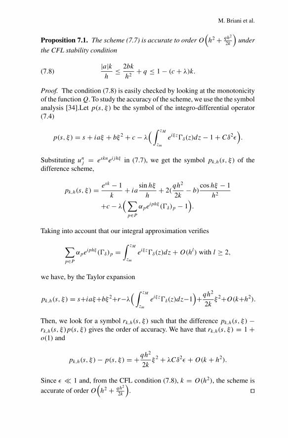
Proposition 7.1. The scheme (7.7) is accurate to orderO(h2 + qh2

2k

)under

the CFL stability condition

|a|kh

≤ 2bk

h2+ q ≤ 1 − (c + λ)k.(7.8)

Proof. The condition (7.8) is easily checked by looking at the monotonicityof the functionQ. To study the accuracy of the scheme, we use the the symbolanalysis [34].Let p(s, ξ) be the symbol of the integro-differential operator(7.4)

p(s, ξ) = s + iaξ + bξ 2 + c − λ( ∫ zM

zm

eiξz�δ(z)dz− 1 + Cδ2ε).

Substituting unj = eskneijhξ in (7.7), we get the symbol pk,h(s, ξ) of thedifference scheme,

pk,h(s, ξ) = esk − 1

k+ ia

sin hξ

h+ 2(

qh2

2k− b)

coshξ − 1

h2

+c − λ( ∑p∈P

αpeiphξ (�δ)p − 1

).

Taking into account that our integral approximation verifies

∑p∈P

αpeiphξ (�δ)p =

∫ zM

zm

eiξz�δ(z)dz+O(hl) with l ≥ 2,

we have, by the Taylor expansion

pk,h(s, ξ) = s+iaξ+bξ 2+r−λ( ∫ zM

zm

eiξz�δ(z)dz−1)+qh

2

2kξ 2+O(k+h2).

Then, we look for a symbol rk,h(s, ξ) such that the difference pk,h(s, ξ) −rk,h(s, ξ)p(s, ξ) gives the order of accuracy. We have that rk,h(s, ξ) = 1 +o(1) and

pk,h(s, ξ)− p(s, ξ) = +qh2

2kξ 2 + λCδ2ε +O(k + h2).

Since ε � 1 and, from the CFL condition (7.8), k = O(h2), the scheme is

accurate of order O(h2 + qh2

2k

). ��

Convergence of numerical schemes arising in financial theory

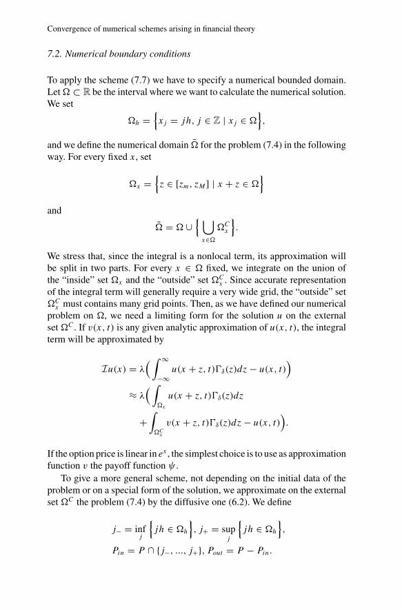
7.2. Numerical boundary conditions

To apply the scheme (7.7) we have to specify a numerical bounded domain.Let� ⊂ R be the interval where we want to calculate the numerical solution.We set

�h ={xj = jh, j ∈ Z | xj ∈ �

},

and we define the numerical domain � for the problem (7.4) in the followingway. For every fixed x, set

�x ={z ∈ [zm, zM ] | x + z ∈ �

}

and

� = � ∪{ ⋃x∈�

�Cx

}.

We stress that, since the integral is a nonlocal term, its approximation willbe split in two parts. For every x ∈ � fixed, we integrate on the union ofthe “inside” set �x and the “outside” set �Cx . Since accurate representationof the integral term will generally require a very wide grid, the “outside” set�Cx must contains many grid points. Then, as we have defined our numericalproblem on �, we need a limiting form for the solution u on the externalset �C . If v(x, t) is any given analytic approximation of u(x, t), the integralterm will be approximated by

Iu(x) = λ( ∫ ∞

−∞u(x + z, t)�δ(z)dz− u(x, t)

)

≈ λ( ∫

�x

u(x + z, t)�δ(z)dz

+∫�Cx

v(x + z, t)�δ(z)dz− u(x, t)).

If the option price is linear in ex , the simplest choice is to use as approximationfunction v the payoff function ψ .

To give a more general scheme, not depending on the initial data of theproblem or on a special form of the solution, we approximate on the externalset �C the problem (7.4) by the diffusive one (6.2). We define

j− = infj

{jh ∈ �h

}, j+ = sup

j

{jh ∈ �h

},

Pin = P ∩ {j−, ..., j+}, Pout = P − Pin.

M. Briani et al.

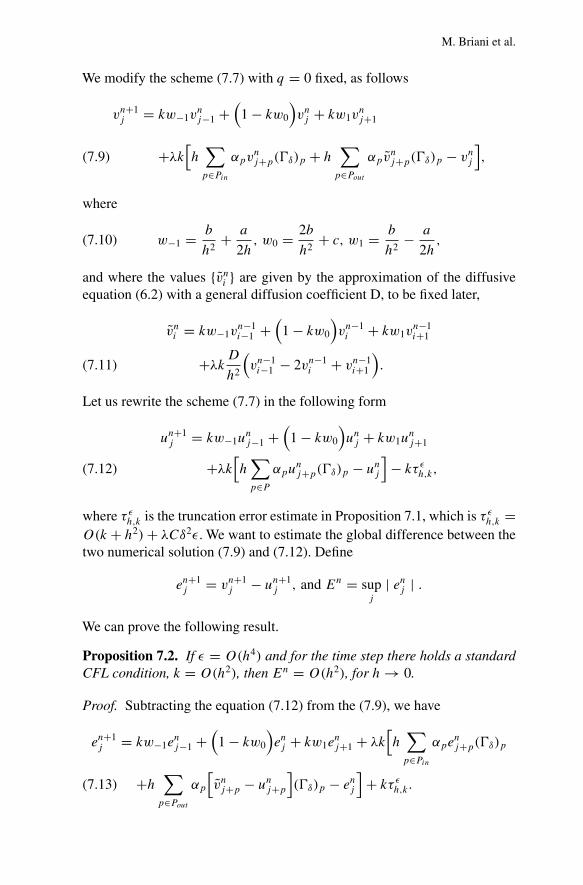
We modify the scheme (7.7) with q = 0 fixed, as follows

vn+1j = kw−1v

nj−1 +

(1 − kw0

)vnj + kw1v

nj+1

+λk[h

∑p∈Pin

αpvnj+p(�δ)p + h

∑p∈Pout

αpvnj+p(�δ)p − vnj

],(7.9)

where

w−1 = b

h2+ a

2h, w0 = 2b

h2+ c, w1 = b

h2− a

2h,(7.10)

and where the values {vni } are given by the approximation of the diffusiveequation (6.2) with a general diffusion coefficient D, to be fixed later,

vni = kw−1vn−1i−1 +

(1 − kw0

)vn−1i + kw1v

n−1i+1

+λk Dh2

(vn−1i−1 − 2vn−1

i + vn−1i+1

).(7.11)

Let us rewrite the scheme (7.7) in the following form

un+1j = kw−1u

nj−1 +

(1 − kw0

)unj + kw1u

nj+1

+λk[h

∑p∈P

αpunj+p(�δ)p − unj

]− kτ εh,k,(7.12)

where τ εh,k is the truncation error estimate in Proposition 7.1, which is τ εh,k =O(k + h2)+ λCδ2ε. We want to estimate the global difference between thetwo numerical solution (7.9) and (7.12). Define

en+1j = vn+1

j − un+1j , and En = sup

j

| enj | .

We can prove the following result.

Proposition 7.2. If ε = O(h4) and for the time step there holds a standardCFL condition, k = O(h2), then En = O(h2), for h → 0.

Proof. Subtracting the equation (7.12) from the (7.9), we have

en+1j = kw−1e

nj−1 +

(1 − kw0

)enj + kw1e

nj+1 + λk

[h

∑p∈Pin

αpenj+p(�δ)p

+h∑p∈Pout

αp

[vnj+p − unj+p

](�δ)p − enj

]+ kτ εh,k.(7.13)

Convergence of numerical schemes arising in financial theory

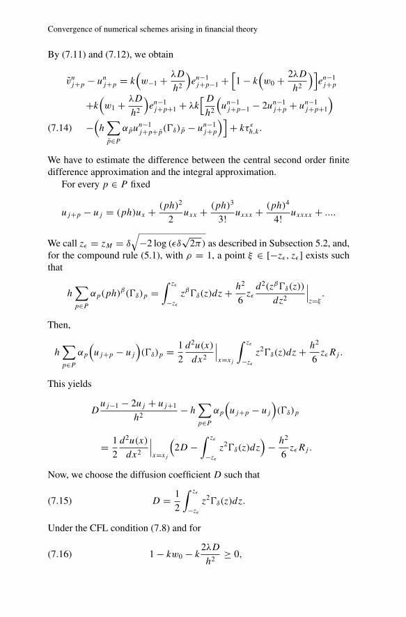
By (7.11) and (7.12), we obtain

vnj+p − unj+p = k(w−1 + λD

h2

)en−1j+p−1 +

[1 − k

(w0 + 2λD

h2

)]en−1j+p

+k(w1 + λD

h2

)en−1j+p+1 + λk

[Dh2

(un−1j+p−1 − 2un−1

j+p + un−1j+p+1

)

−(h

∑p∈P

αpun−1j+p+p(�δ)p − un−1

j+p)]

+ kτ εh,k.(7.14)

We have to estimate the difference between the central second order finitedifference approximation and the integral approximation.

For every p ∈ P fixed

uj+p − uj = (ph)ux + (ph)2

2uxx + (ph)3

3!uxxx + (ph)4

4!uxxxx + ....

We call zε = zM = δ

√−2 log (εδ

√2π) as described in Subsection 5.2, and,

for the compound rule (5.1), with ρ = 1, a point ξ ∈ [−zε, zε] exists suchthat

h∑p∈P

αp(ph)β(�δ)p =

∫ zε

−zεzβ�δ(z)dz+ h2

6zεd2(zβ�δ(z))

dz2

∣∣∣z=ξ.

Then,

h∑p∈P

αp

(uj+p − uj

)(�δ)p = 1

2

d2u(x)

dx2

∣∣∣x=xj

∫ zε

−zεz2�δ(z)dz+ h2

6zεRj .

This yields

Duj−1 − 2uj + uj+1

h2− h

∑p∈P

αp

(uj+p − uj

)(�δ)p

= 1

2

d2u(x)

dx2

∣∣∣x=xj

(2D −

∫ zε

−zεz2�δ(z)dz

)− h2

6zεRj .

Now, we choose the diffusion coefficient D such that

D = 1

2

∫ zε

−zεz2�δ(z)dz.(7.15)

Under the CFL condition (7.8) and for

1 − kw0 − k2λD

h2≥ 0,(7.16)

M. Briani et al.

from (7.13) and (7.14), we have

En+1 ≤[1 − kc + λkh

∑p∈Pin

(�δ)p − λk]En

+[λk

(1 − kc

)h

∑p∈Pout

αp(�δ)p

]En−1

+λ2k2h2

6zεh

∑p∈Pout

αp | Rj+p | (�δ)p

+λk2 | τ εh,k | h∑p∈Pout

αp(�δ)p + k | τ εh,k | .

This is, for some coefficients A, B and C,

En+1 ≤ AEn + BEn−1 + C.(7.17)

As a consequence, for any n+12 ≤ m < n we have

En+1 ≤ En−2m+1m∑k=0

(m

k

)(AE)kBm−k + C

m−1∑k=0

(A+ B)k.

When n− 2m+ 1 = 0, E0 = 0 it yields

En+1 ≤ C1 − (A+ B)

n+12

1 − (A+ B).(7.18)

Now, we have

h∑

p∈Pin,Pout(�δ)p ≤ 2zε max

z�δ = 2zε� and | Rj |≤ R.

The CFL condition (7.16) gives k = O(h2) and τ εh,k = O(h2 + ε). Then, forN = T/k, the global error (7.18) is estimated by

EN ≤(

1 − T

Nc − 2

T 2

N2λzε�

)N/2g(h, ε),

where

g(h, ε) = O(h4z2

ε + h4zε + h2εzε + h2 + ε

1 + h2zε

).

As h and k go to zero, we obtain

limN→∞

(A+ B)N/2 =(

1 − T

Nc − 2

T 2

N2λzε�

)N/2= e

TC2 .

Convergence of numerical schemes arising in financial theory

Then, to get the rate of convergence as h → 0, we observe that the minimalvalue of the function g(·, ε) is achieved for ε = O(h4).

Therefore, the conclusion follows, since

limN→∞

EN ≤ eTC2 g(h, h4) ≤ e

TC2

(− h4 logh4 + h4

√− logh4

+h6√

− logh4 + h2 + h4)

= O(h2).

��Remark 7.3. We point out that, for the Gaussian probability density (2.2) wehave

k = E(η − 1) = exp(δ2

2

)− 1 ≈ δ2

2+O(δ4), δ � 1,

then, solving the approximated problem (6.2) in�C is just solving the Black-Scholes equation (7.1) with coefficients

a = σ 2

2− r + λk ≈ σ 2

2− r + λ

δ2

2, b = σ 2

2+ λ

δ2

2.

Even if the scheme (7.9) needs for a CFL condition and its convergencein time is only first order accurate, we shall see in Subsection 8.1 that it isof simple practice application and computationally fast. It is easy to obtain ascheme which is second order in time, by applying the SSP (Strong StabilityPreserving) Runge-Kutta technique, as in [24] and references therein, but weobserve no real advantages for the total accuracy at least for the second ordercase. Then in what follows, we just use scheme (7.9).

8. Examples and Numerical tests

In this section we compute the order γ of the error in the following form

γ = log2

(e1

e2

),(8.1)

with

ep =‖ u( h

p, T )− u( h2p , T ) ‖1,∞

‖ u( h2p , T ) ‖1,∞, p = 1, 2,(8.2)

where u(h) denotes the numerical solution obtained with the space step dis-cretization equal to h, under the discrete norm l1 and l∞, respectively

‖ u(·, T ) ‖1= h∑i

| u(xi, T ) |, ‖ u(·, T ) ‖∞= maxi | u(xi, T ) | .

If not specified, in tables that follow we give the average convergence order.

M. Briani et al.

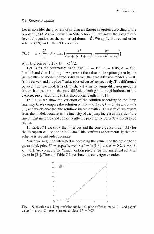
8.1. European option

Let us consider the problem of pricing an European option according to theproblem (7.4). As we showed in Subsection 7.1, we solve the integro-dif-ferential equation on the numerical domain �. We apply the second orderscheme (7.9) under the CFL condition

h ≤ 2b

a, k ≤ min

( h2

2b + 2λD + ch2,

h2

2b + ch2 + λh2

),(8.3)

with D given by (7.15), D = λδ2/2.Let us fix the parameters as follows: E = 100, r = 0.05, σ = 0.2,

δ = 0.2 and T = 1. In Fig. 1 we present the value of the option given by thejump-diffusion model (dotted-solid curve), the pure diffusion model (λ = 0)(solid curve), and the payoff value (dotted curve) respectively. The differencebetween the two models is clear: the value in the jump diffusion model islarger than the one in the pure diffusion setting in a neighborhood of theexercise price, according to the theoretical results in [31].

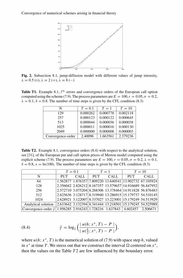
In Fig. 2, we show the variation of the solution according to the jumpintensity λ. We compare the solution with λ = 0.5 (�), λ = 2 (+) and λ = 8(−) and we observe that the solutions increase with λ. This is what we expectfrom the model, because as the intensity of the jump increases the risk of theinvestment increases and consequently the price of the derivative needs to behigher.

In Tables T 1 we show the l∞ errors and the convergence order (8.1) forthe European call option initial data. This confirms experimentally that thescheme is second order accurate.

Since we might be interested in obtaining the value u of the option for agiven stock price S∗ = exp(x∗), we fix x∗ = ln(100) and σ = 0.2, δ = 0.8,λ = 0.1. We compute the “exact” option price P by the analytical solutiongiven in [31]. Then, in Table T 2 we show the convergence order,

0

20

40

60

80

100

120

140

160

50 100 150 200 250

’bs’’jump’

’payoff’

Fig. 1. Subsection 8.1, jump-diffusion model (�), pure diffusion model (−) and payoffvalue (· · · ), with Simpson compound rule and h = 0.05

Convergence of numerical schemes arising in financial theory

0

20

40

60

80

100

120

140

160

50 100 150 200 250

’0.5’’2’’8’

’payoff’

Fig. 2. Subsection 8.1, jump-diffusion model with different values of jump intensity,λ = 0.5 (�), λ = 2 (+), λ = 8 (−)

Table T1. Example 8.1, l∞ errors and convergence orders of the European call optioncomputed using the scheme (7.9). The process parameters areE = 100, r = 0.05,σ = 0.2,λ = 0.1, δ = 0.8. The number of time steps is given by the CFL condition (8.3)

N T = 0.1 T = 1 T = 10129 0.000262 0.000778 0.002118257 0.000123 0.000122 0.000645513 0.000044 0.000036 0.0000381025 0.000011 0.000016 0.0001302049 0.000000 0.000008 0.000003

Convergence-order 2.40096 1.663561 2.379236

Table T2. Example 8.1, convergence orders (8.4) with respect to the analytical solution,see [31], of the European put and call option prices of Merton model computed using theexplicit scheme (7.9). The process parameters are E = 100, r = 0.05, σ = 0.2, λ = 0.1,δ = 0.8, x = ln(100). The number of time steps is given by the CFL condition (8.3)

T = 0.1 T = 1 T = 10N PUT CALL PUT CALL PUT CALL64 1.562877 1.876357 7.809220 13.640541 13.902732 67.105924

128 2.356042 2.826212 8.167357 13.579657 14.916689 56.847952256 2.572710 3.075204 8.268306 13.378464 14.911828 56.876483512 2.625636 3.128717 8.319940 13.286915 15.179737 54.5101451024 2.628921 3.122007 8.337027 13.223001 15.179249 54.513929

Analytical solution 2.633642 3.132394 8.341444 13.218501 15.179245 54.525989Convergence-order γ 1.956285 2.916243 1.728216 1.637843 4.602457 2.506671

γ = log2

( | u(h; x∗, T )− P || u(h2 ; x∗, T )− P |

),(8.4)

where u(h; x∗, T ) is the numerical solution of (7.9) with space step h, valuedin x∗ at time T . We stress out that we construct the interval� centered on x∗,then the values on the Table T 2 are few influenced by the boundary error.

M. Briani et al.

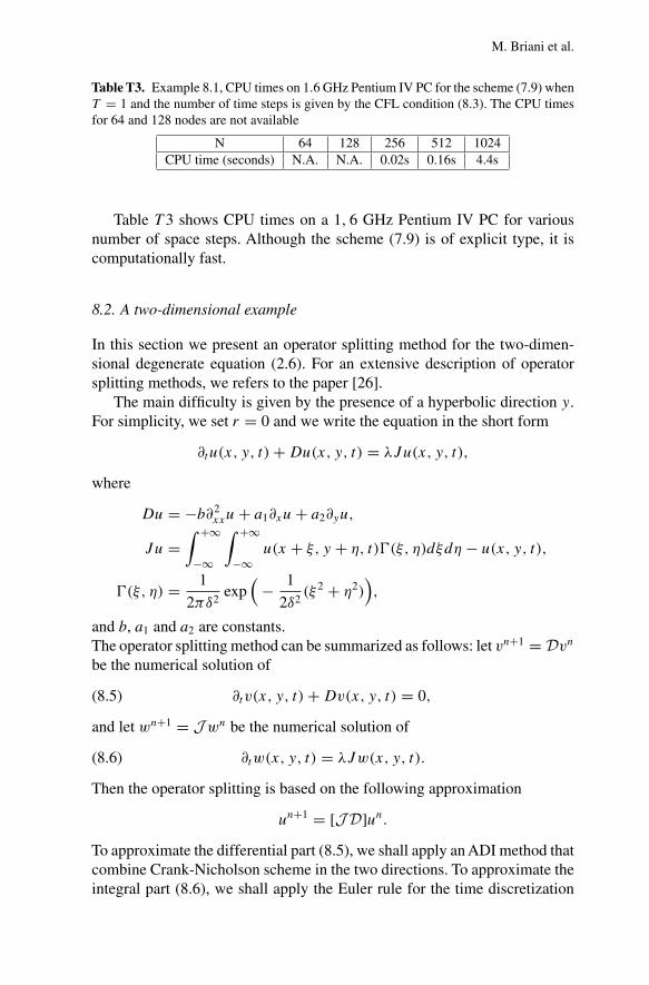
Table T3. Example 8.1, CPU times on 1.6 GHz Pentium IV PC for the scheme (7.9) whenT = 1 and the number of time steps is given by the CFL condition (8.3). The CPU timesfor 64 and 128 nodes are not available

N 64 128 256 512 1024CPU time (seconds) N.A. N.A. 0.02s 0.16s 4.4s

Table T 3 shows CPU times on a 1, 6 GHz Pentium IV PC for variousnumber of space steps. Although the scheme (7.9) is of explicit type, it iscomputationally fast.

8.2. A two-dimensional example

In this section we present an operator splitting method for the two-dimen-sional degenerate equation (2.6). For an extensive description of operatorsplitting methods, we refers to the paper [26].

The main difficulty is given by the presence of a hyperbolic direction y.For simplicity, we set r = 0 and we write the equation in the short form

∂tu(x, y, t)+Du(x, y, t) = λJu(x, y, t),

where

Du = −b∂2xxu+ a1∂xu+ a2∂yu,

Ju =∫ +∞

−∞

∫ +∞

−∞u(x + ξ, y + η, t)�(ξ, η)dξdη − u(x, y, t),

�(ξ, η) = 1

2πδ2exp

(− 1

2δ2(ξ 2 + η2)

),

and b, a1 and a2 are constants.The operator splitting method can be summarized as follows: let vn+1 = Dvnbe the numerical solution of

∂tv(x, y, t)+Dv(x, y, t) = 0,(8.5)

and let wn+1 = Jwn be the numerical solution of

∂tw(x, y, t) = λJw(x, y, t).(8.6)

Then the operator splitting is based on the following approximation

un+1 = [J D]un.

To approximate the differential part (8.5), we shall apply an ADI method thatcombine Crank-Nicholson scheme in the two directions. To approximate theintegral part (8.6), we shall apply the Euler rule for the time discretization

Convergence of numerical schemes arising in financial theory

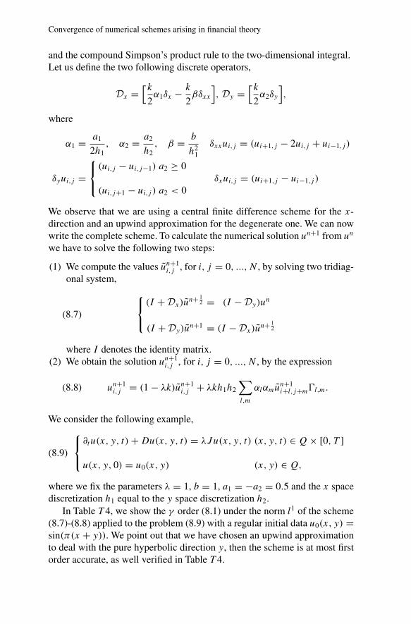
and the compound Simpson’s product rule to the two-dimensional integral.Let us define the two following discrete operators,

Dx =[k

2α1δx − k

2βδxx

], Dy =

[k2α2δy

],

where

α1 = a1

2h1, α2 = a2

h2, β = b

h21

δxxui,j = (ui+1,j − 2ui,j + ui−1,j )

δyui,j =(ui,j − ui,j−1) a2 ≥ 0

(ui,j+1 − ui,j ) a2 < 0δxui,j = (ui+1,j − ui−1,j )

We observe that we are using a central finite difference scheme for the x-direction and an upwind approximation for the degenerate one. We can nowwrite the complete scheme. To calculate the numerical solution un+1 from un

we have to solve the following two steps:

(1) We compute the values un+1i,j , for i, j = 0, ..., N , by solving two tridiag-

onal system,

(I + Dx)u

n+ 12 = (I − Dy)u

n

(I + Dy)un+1 = (I − Dx)u

n+ 12

(8.7)

where I denotes the identity matrix.(2) We obtain the solution un+1

i,j , for i, j = 0, ..., N , by the expression

un+1i,j = (1 − λk)un+1

i,j + λkh1h2

∑l,m

αlαmun+1i+l,j+m�l,m.(8.8)

We consider the following example,∂tu(x, y, t)+Du(x, y, t) = λJu(x, y, t) (x, y, t) ∈ Q× [0, T ]

u(x, y, 0) = u0(x, y) (x, y) ∈ Q,(8.9)

where we fix the parameters λ = 1, b = 1, a1 = −a2 = 0.5 and the x spacediscretization h1 equal to the y space discretization h2.

In Table T 4, we show the γ order (8.1) under the norm l1 of the scheme(8.7)-(8.8) applied to the problem (8.9) with a regular initial data u0(x, y) =sin(π(x + y)). We point out that we have chosen an upwind approximationto deal with the pure hyperbolic direction y, then the scheme is at most firstorder accurate, as well verified in Table T 4.

M. Briani et al.

TableT4. Convergence order γ , defined in (8.1), and errors, for the solution of the problem(8.9) with u0(x, y) = sin(π(x + y)), b = 1, a1 = −a2 = 0.5

δ = 10−4 δ = 10−2

h1 = h2 γ ep γ ep0.025 0.099739 0.089381

0.0125 1.308349 0.040273 1.485643 0.0319170.00625 0.557111 0.027372 0.9416737 0.016169

0.003125 0.9288881 0.014378 0.447856 0.011854

8.3. The nonlinear case

As we have already seen in Section 2, the option pricing in large investoreconomy leads to a quasilinear differential problem. From equation (2.4),by the standard change of variable x = log S, we get the following generalequation

ut + LIuu = H(x, t, u, Iu,Du),where LI is a linear degenerate elliptic integro-differential operator and His a nonlinear integro-differential Hamilton-Jacobi operator.

The numerical approximation of Hamilton-Jacobi equations has beenintensively studied, both for first and second order equations. We refer againto [16,9] for classical results and to [32,29,28] for recent developments ofhigh order accurate schemes, such as ENO, WENO, and central schemes.

Let us introduce some standard notations:

u± = �±uj = ±(uj±1 − uj )

h,

�2uj = uj+1 − 2uj + uj−1

h2, H (u+, u−),

where H is a Lipschitz continuous numerical flux, which is monotone andconsistent with H [16], i.e.:

H (p, p) = H(p).

Monotonicity here means that H in non-increasing in its first argument andnondecreasing in the other one. Two of the most useful admissible numericalfluxes are the local Lax-Friedrichs (LLF) flux and the Godunov flux, [32].

Example 8.1. [Large institutional investor]. Let us consider the Merton modelfor the large investor economy. As we have seen in the Example 2.1, the inter-est rate r depends on the wealth ξ invested in stocks and the price functionsolves the quasi-linear final value problem (2.4). In the specific case of thelarge institutional investor, the interest rate decreases when too much wealthis invested in bonds, according to the law r(S, t, ξ) = R(S, t)f (ξ) where fis a positive continuous function such that, for a given wealth ξ0 ≥ 0 fixed,

Convergence of numerical schemes arising in financial theory

f (ξ) = 1 as ξ ≤ ξ0 and f is decreasing as ξ > ξ0, but f (ξ)ξ non decreasing.A good prototype of such type function f is given by

f (ξ) =

1, ξ ≤ ξ0

α + βξ0ξ−γ ξ > ξ0,

for all α, β and γ such that α, β > 0, 0 < γ ≤ 1 and α + βξ−γ+10 = 1. We

select,

γ = 12 , β = 1

2√ξ0

⇒ α = 12 ,

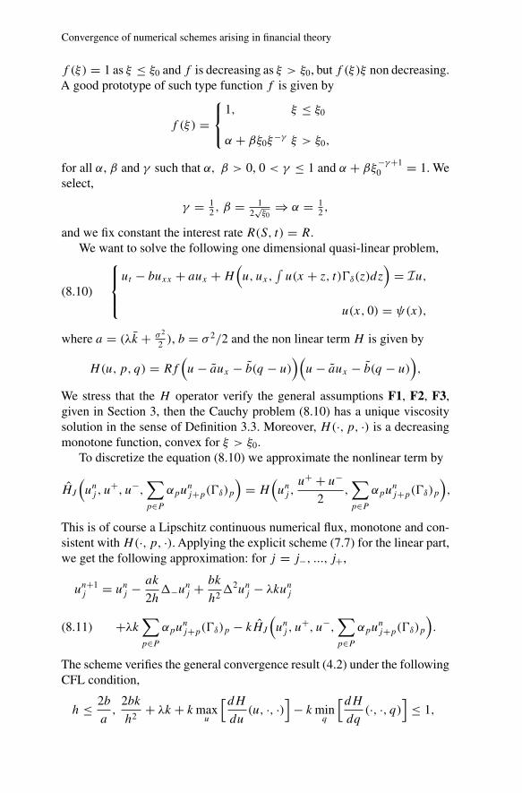
and we fix constant the interest rate R(S, t) = R.We want to solve the following one dimensional quasi-linear problem,

ut − buxx + aux +H

(u, ux,

∫u(x + z, t)�δ(z)dz

)= Iu,

u(x, 0) = ψ(x),

(8.10)

where a = (λk + σ 2

2 ), b = σ 2/2 and the non linear term H is given by

H(u, p, q) = Rf(u− aux − b(q − u)

)(u− aux − b(q − u)

),

We stress that the H operator verify the general assumptions F1, F2, F3,given in Section 3, then the Cauchy problem (8.10) has a unique viscositysolution in the sense of Definition 3.3. Moreover, H(·, p, ·) is a decreasingmonotone function, convex for ξ > ξ0.

To discretize the equation (8.10) we approximate the nonlinear term by

HJ

(unj , u

+, u−,∑p∈P

αpunj+p(�δ)p

)= H

(unj ,

u+ + u−

2,∑p∈P

αpunj+p(�δ)p

),

This is of course a Lipschitz continuous numerical flux, monotone and con-sistent withH(·, p, ·). Applying the explicit scheme (7.7) for the linear part,we get the following approximation: for j = j−, ..., j+,

un+1j = unj − ak

2h�−unj + bk

h2�2unj − λkunj

+λk∑p∈P

αpunj+p(�δ)p − kHJ

(unj , u

+, u−,∑p∈P

αpunj+p(�δ)p

).(8.11)

The scheme verifies the general convergence result (4.2) under the followingCFL condition,

h ≤ 2b

a,

2bk

h2+ λk + kmax

u

[dHdu

(u, ·, ·)]

− kminq

[dHdq

(·, ·, q)]

≤ 1,

M. Briani et al.

As it has been done for the linear problem (7.4), on the numerical bound-ary domain�C we approximate the integral term Iu in (8.10) by the diffusiveone Duxx and we solve the following equation,

ut − buxx + aux +H(u, ux,Duxx

)= λDuxx, (x, t) ∈ �C × (0, T ],

under the condition

2bk

h2+ 2λDk

h2+ kmax

u

[dHdu

(u, ·, ·)]

−Dkminq

[dHdq

(·, ·, q)]

≤ 1.(8.12)

We fix a = a, b = b, the parameters E = 100, R = 0.05, σ = 0.2,λ = 0.1, δ = 0.4 and the initial data ψ(x) = (ex − E)+ as the call optionpayoff function.

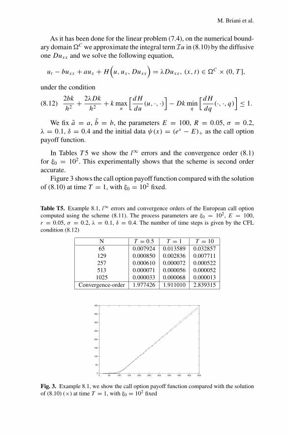
In Tables T 5 we show the l∞ errors and the convergence order (8.1)for ξ0 = 102. This experimentally shows that the scheme is second orderaccurate.

Figure 3 shows the call option payoff function compared with the solutionof (8.10) at time T = 1, with ξ0 = 102 fixed.

Table T5. Example 8.1, l∞ errors and convergence orders of the European call optioncomputed using the scheme (8.11). The process parameters are ξ0 = 102, E = 100,r = 0.05, σ = 0.2, λ = 0.1, δ = 0.4. The number of time steps is given by the CFLcondition (8.12)

N T = 0.5 T = 1 T = 1065 0.007924 0.013589 0.032857129 0.000850 0.002836 0.007711257 0.000610 0.000072 0.000522513 0.000071 0.000056 0.0000521025 0.000033 0.000068 0.000013

Convergence-order 1.977426 1.911010 2.839315

0

50

100

150

200

250

300

350

400

0 50 100 150 200 250 300 350 400 450 500

Fig. 3. Example 8.1, we show the call option payoff function compared with the solutionof (8.10) (×) at time T = 1, with ξ0 = 102 fixed

Convergence of numerical schemes arising in financial theory

Acknowledgements. The first two authors would like to thank the whole staff of IAC-CNRfor their kind hospitality during the development of this work.

References

1. Ait-Sahalia,Y., Wang,Y.,Yared, F.: Do option markets correctly price the probabilitiesof movements of the underlying asset?. Working paper, Univ. of Chicago, 1998

2. Alvarez, O., Tourin,A.:Viscosity solutions of nonlinear integro-differential equations.Ann. Inst. Henri Poincare Anal. Non Lineaire 13(3), 293–317 (1996)

3. Amadori, A.L.: Differential And Integro–Differential Nonlinear Equations of Degen-erate Parabolic Type Arising in the Pricing of Derivatives in Incomplete Markets.Ph.D. Thesis, Universita di Roma “La Sapienza”, 2000

4. Amadori, A.L.: Nonlinear integro-differential evolution problems arising in optionpricing: a viscosity solutions approach. J. Differential and Integral Equations 16(7),787–811 (2003)

5. Amadori,A.L.: The obstacle problem for nonlinear integro–differential operators aris-ing in option pricing Quaderno IAC, Q21-000, (2000)

6. Andersen, L., Andreasen, J.: Jump-Diffusion Processes: volatility smile fitting andnumerical methods for pricing. Rev. Derivative Res. 4, 231–262 (2000)

7. Andersen, L., Benzoni, L., Lund, J.: Estimating jump–diffusions for equity returns.Working paper, Northweterns Univ. and Aarhus School of Business, 1999

8. Attari, M.: Discontinuous interest rate processes: an equilibrium model of bond optionprices. Working paper, Univ. Madison (Winsconsin), 1997

9. Barles, G., Souganidis, P.E.: Convergence of approximation schemes for fully non-linear second order equations. Asymptotic Anal 4(3), 271–283 (1991)

10. Bates, D.: Jumps and stochastic volatility: exchange rate processes implicit in Deutschmark options. Review of financial studies 9, 69–107 (1996)

11. Black, F., Scholes, M.: The pricing of option and corporate liabilities. J. PoliticalEconom. 72, 637–659 (1973)

12. Bjork, T.: Arbitrage Theory in Continuous Time. Oxford: Oxford University Press,1998

13. Bjork, T., Kabanov, Y., Runggaldier, W.: Bond market structure in the presence ofmarked point processes. Math. Finance 7(2), 211–239 (1997)

14. Burneta, A.N., Ritchken, P.: On rational jump-diffusion models in the Flesaker-Hugh-ston paradigm, Working paper, Case western reserves University, 1996

15. Crandall, M.G., Ishi, H., Lions, P.L.: Users’ guide to viscosity solutions of secondorder partial differential equations. Bull. Am. Math. Soc., (New Ser.) 27(1), 1–67(1992)

16. Crandall, M.G., Lions, P.L.: Two approximations of solutions of Hamilton-Jacobiequations. Math. Comput. 43(167), 1–19 (1994)

17. Das, S., Foresi, S.: Exact solutions for bond and option prices with systematic jumprisk. J. Financ. Quantitative Anal. 34, 211–240 (1999)

18. Das, S.R.: The surprise element: jumps in interest rates. J. Econometrics 106(1), 27–65(2002)

19. Davis, P.J., Rabinowitz, P.: Methods of numerical integration. Academic Press, Inc.(1975)

20. Duffie, D., Pan, J., Singleton, K.: Transform analysis and asset pricing for affinejump-diffusions. Econometrica 68(6), 1343–1376 (2000)

21. Garroni, M.G., Menaldi, J.L.: Green functions for second order parabolic integro-dif-ferential problems. Pitman Res. Notes Math. Ser. (1992)

M. Briani et al.

22. Garroni, M.G., Menaldi, J.L.: Regularizing effect for integro-differential parabolicequations. Commun. Partial Differential Equations 18(12), 2023–2025 (1993)

23. Garroni, M.G., Menaldi, J.L.: Maximum principle for integro-differential parabolicoperators. Differ. Integral Equ. 8(1), 161–182 (1995)

24. Gottlieb, S., Shu, C.-W., Tadmor, E.: Strong stability-preserving high-order time dis-cretization methods. SIAM Rev. 43, 89–112 (2001)

25. Jarrow, R., Madan, D.: Option pricing using the term structure of interest rates to hedgesystematic discontinuities in asset returns. Math. Finance 5(4), 311–336 (1995)

26. Karlsen, K.H., Risebro, N.H.: An operator splitting method for nonlinear convection-diffusion equations. Numer. Math. 77(3), 365–382 (1997)

27. Kou, S.G.:A jump diffusion model for option pricing. Management Science 48, 1086–1101 (2002)

28. Kurganov, A., Tadmor, E.: New High-Resolution Semi-Discrete Central Schemes forHamilton-Jacobi Equations. J. Comput. Phys. 160(2), 720–742 (2000)

29. Lin, C.-T., Tadmor, E.: High-resolution non-oscillatory central scheme for Hamilton-Jacobi equations. SIAM J. Sci. Comput. 21, 2163–2186 (2000)

30. Magill, M., Quinzii, M.: Theory of incomplete markets. vol. 1 – MIT Press, 199631. Merton, R.C.: Option pricing when the underlying stocks returns are discontinuous.

J. Financ. Econ. 5, 125–144 (1976)32. Osher, S., Shu, C.-W.: High-order essentially non-oscillatory schemes for Hamilton-

Jacobi equations. SIAM J. Numer. Anal. 28(4), 907–922 (1991)33. Page, F.H., Sanders, A.B.: A general derivation of the jump process option pricing

formula. J. Financial and Quantitative Anal. 21, 437–446 (1986)34. Strikwerda, J.C.: Finite Difference Schemes and Partial Differential Equations. Chap-

man & Hall, New York35. Tavella, D., Randall, C.: Pricing financial instruments - the finite difference method.

John Wiley & Sons, Inc. 200036. Yong, J., Zhou, X.Y.: Stochastic controls. Hamiltonian systems and HJB equations.

Applications of Mathematics, 43. New York: Springer-Verlag, 1999