This is a postprint version of the following document:

Martín-Peréz, J., Malandrino,F., Chiasserini,C. F., Bernardos, C. J.(2020). OKpi: All-KPI Network Slicing Through Efficient Resource Allocation. In IEEE INFOCOM 2020 - IEEE Conference on Computer Communications, pp. 804-813.

DOI: https://doi.org/10.1109/INFOCOM41043.2020.9155263

© 2020 IEEE. Personal use of this material is permitted. Permission from IEEE must be obtained for all other uses, in any current or future media, including reprinting/republishing this material for advertising or promotional purposes, creating new collective works, for resale or redistribution to servers or lists, or reuse of any copyrighted component of this work in other works.

OKpi: All-KPI Network SlicingThrough Efficient Resource Allocation

J. Martın-Perez†, F. Malandrino‡,§, C. F. Chiasserini∗,‡,§, C. J. Bernardos†

† Universidad Carlos III de Madrid, Spain – ‡ CNR-IEIIT, Italy – ∗ Politecnico di Torino, Italy – § CNIT, Italy

Abstract—Networks can now process data as well as trans-porting it; it follows that they can support multiple services,each requiring different key performance indicators (KPIs).Because of the former, it is critical to efficiently allocate networkand computing resources to provide the required services, and,because of the latter, such decisions must jointly consider allKPIs targeted by a service. Accounting for newly introducedKPIs (e.g., availability and reliability) requires tailored modelsand solution strategies, and has been conspicuously neglected byexisting works, which are instead built around traditional metricslike throughput and latency. We fill this gap by presenting a novelmethodology and resource allocation scheme, named OKpi, whichenables high-quality selection of radio points of access as well asVNF (Virtual Network Function) placement and data routing,with polynomial computational complexity. OKpi accounts forall relevant KPIs required by each service, and for any availableresource from the fog to the cloud. We prove several importantproperties of OKpi and evaluate its performance in two real-world scenarios, finding it to closely match the optimum.

I. INTRODUCTION

Network Function Virtualization (NFV) enables mobile net-works to expand their capabilities beyond data transport and tosupport software-based applications on demand. Under sucha paradigm, third party industries (“verticals”) specify theirservices through a graph of virtual network functions (VNFs),then it is the mobile network’s task to run such services. Thisrequires selecting suitable radio points of access (PoAs) aswell as placing and connecting the VNFs across computingand network resources1, in order to deliver the vertical serviceswith the required quality of service. Importantly, differentresources can be employed to achieve this goal, ranging fromthose in the cloud to the ones at the edge of the network infras-tructure (i.e., through multi-access edge computing (MEC))or in the fog (i.e., in devices such as smartphones, vehicles,robots). Note that which and how many resources are usedis a critical issue, as their associated cost, performance, andavailability vary significantly. This is confirmed by [1]–[4],highlighting how cost is a grave concern for both the mobileoperators owning the cellular infrastructure and the verticalspaying for the services mobile systems should support.In spite of the fact that the VNF placement problem has

been already addressed in the literature (see Sec. II for amore in-depth discussion), virtually all existing approachesonly focus on throughput and latency as performance metrics,ignoring what is one of the most disruptive innovations of

1Although memory and storage resources have been omitted for brevity,our framework can handle them as well.

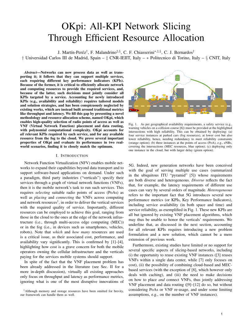
Fig. 1. As per geographical availability requirements, a safety service (e.g.,warning vehicles on a collision course [6]) must be provided at the highlightedintersections with high reliability. This can be obtained by deploying: (a)four service instances at parked cars (fog resources), at lower cost but alsolower reliability, hence, needing redundancy to meet reliability constraints(orange option); (b) three instances at the points of access (PoA), e.g., eNBs,covering the intersections (MEC resources, blue option); (c) deploying onlyone instance in the cloud, but with larger delay (green option).

5G. Indeed, new generation networks have been conceivedwith the goal of serving multiple use cases (summarizedin the ubiquitous ITU “pyramid” [5]) whose requirementsare both diverse and heterogeneous. Diverse reflects the factthat, for example, the latency requirements of different usecases can vary by several orders of magnitude. Heterogeneousrefers to the important fact that 5G introduces several newperformance metrics (or KPIs, Key Performance Indicators),including service availability (in both space and time) andservice reliability, as exemplified in Fig. 1. These new KPIs areall but ignored by existing VNF placement algorithms, whichmay thus be unable to honor the verticals’ requirements. Weunderline that, as discussed in the next section, accountingfor all relevant KPIs requires introducing a new problemformulation and a new solution, which cannot be a mereextension of previous work.Furthermore, existing studies have limited or no support for

several specific aspects of slicing-based networks, including(i) the opportunity to reuse existing VNF instances ([3] reusesVNFs within a single data center, while [7] only focuses oncost), (ii) the possibility of combining cloud-based and MEC-based services (with the exception of [8], which however onlydeals with caching), and (iii) the need to make decisionson how to place and connect VNFs, thus jointly addressingVNF placement and data routing ([9]–[12] do so, but withoutconsidering PoAs or VNF re-usage, and under some limitingassumptions, e.g., on the number of VNF instances).

1

Our contribution and methodology. We fill this gap byintroducing OKpi, an efficient framework able to create high-quality, end-to-end network slices. Specifically, OKpi advancesthe state-of-the-art in the following main ways:(i) it effectively tackles the 5G-defined network slicing KPIs;(ii) it leverages fog, MEC, and cloud resources, allowing

VNFs to be placed at any layer of the network topology;(iii) it accounts for the fact that already-deployed VNF in-

stances can be reused for newly-requested services2;(iv) in such a general setting, it makes joint decisions on

PoA selection, VNF placement, and traffic routing, whichminimize the cost of the resources, thus addressing bothmobile operators and verticals’ concerns;

(v) it exhibits a low, namely, polynomial, complexity.We remark that, not only the problem we pose is novel,but also our methodology to solve it blends together graphtheory and optimization, in a unique fashion. In particular,we describe possible decisions through a graph that reflectstheir effect on KPIs. Such a graph is then translated into amulti-dimensional expanded graph, which allows us to effi-ciently find feasible decisions leveraging simple shortest-pathalgorithms. The expanded graph can be built with differentlevels of detail and size, which results into a tuneable tradeoffbetween computational complexity and optimality.In the remainder of the paper, we first review related works

in Sec. II, highlighting which KPIs they consider and thenovelty of our study. After that, we introduce the system modelin Sec. III, and the problem formulation in Sec. IV. The OKpisolution and algorithm are described in Sec. V; then Sec. VIproves several relevant properties of OKpi and discusses itscomputational complexity. Sec. VII compares OKpi againstthe optimum in a small-scale, yet practically relevant roboticsscenario, and shows its performance in a real-world, large-scale automotive scenario. Finally, Sec. VIII concludes thepaper and highlights current research directions.

II. RELATED WORK

One of the pioneering works on VNF placement is [13],which casts placement as a generalized assignment problem(GAP) and proposes a near-optimal solution based on bi-criteria approximation. Very recent works [10], [12], [14]focus on the mutual influence of VNF placement and trafficrouting. Others tackle the VNF placement problem throughgraph theory [9], [15] and set-covering [4], obtaining verygood competitive ratios (constant in specific cases for [4]).In the context of MEC, some works tackle tasks different

from sheer data processing; as an example, [11], [16] aimat jointly optimizing computation and caching offloadingbetween cloud-based and MEC-based infrastructure. Othersfocus on additional decisions that can be made in slicing sce-narios, e.g., priority assignment in [3]. A body of works con-siders incremental deployment, i.e., service requests arrivingat different times: in this case, it is possible to share existing

2This is possible if the services share a common subset of VNFs and noservice isolation constraints exist.

VNF instances [3], [7], [17], augment routing paths instead ofcomputing them from scratch [7], [17], and minimize the dif-ference between current and future network configuration [17].Among the few works tackling non-functional requirements,[2] performs resilient VNF placement, to achieve robustness toequipment failures. More recently, [18] considered the problemof jointly placing the VNFs and the data they need.VNF placement, along with the closely-related problem of

VNF chaining, has been studied in the software-defined net-working and cloud-computing contexts as well. For instance,[19] focuses on updating the placement in order to react totraffic changes, and [20] deals with the parallelization oppor-tunities offered by VNF graphs. Other works [10], [21] focuson the choice between MEC- and cloud-based computationresources, while [8] studies which cache storage (i.e., MEC-or cloud-based) to access, balancing miss probability and cost.Several works aim at simplifying the problem of VNF

placement by characterizing and/or predicting the traffic de-mand. In particular, [22] exploits the spatial and temporalvariability of traffic demand to serve it with as little resourcesas possible; as for demand prediction, popular approachesinclude reinforcement learning [23]. In a similar spirit, [24]estimates the resources needed by an incoming service requestbefore deciding whether or not it shall be accepted.Finally, a body of work addresses the slicing of the radio

access network; in particular, [25] proposes solutions that letdifferent virtual operators use the radio resources without inter-fering, while [26] develops a stochastic model to investigatethe throughput and delay of a slice as functions of the cellparameters. Although such specific aspects are out of the scopeof our work, we do tackle the problem of selecting radiotechnologies and points of access that honor the required KPItargets and minimize the cost.Novelty. Remarkably, none of the existing works accounts

for fundamental KPIs in network slicing such as availabilityor reliability: due to their pioneering nature, such works focuson traditional performance metrics, namely, service latencyand/or network throughput. Although some approaches couldbe extended to account for additional KPIs, such extensionswould not be trivial and would, in general, jeopardize theircomplexity and/or competitive ratio properties. OKpi, on thecontrary, is designed from the start to support multiple, het-erogeneous KPIs in an effective and efficient manner, besideaccounting for all types of resources and their location, fromthe fog to the cloud. Our methodology combining graph theoryand optimization is also unique, and provides an effective wayto tradeoff optimality and complexity.

III. SYSTEM MODEL

Our model concisely describes the two main componentsof mobile, slicing-based networks: the services they support(Sec. III-A), and the computing and network resources theyinclude (Sec. III-B). Each of them is modeled through a graph– the service graph and the physical graph, respectively. Wethen describe how such graphs can be combined in Sec. III-C.

2

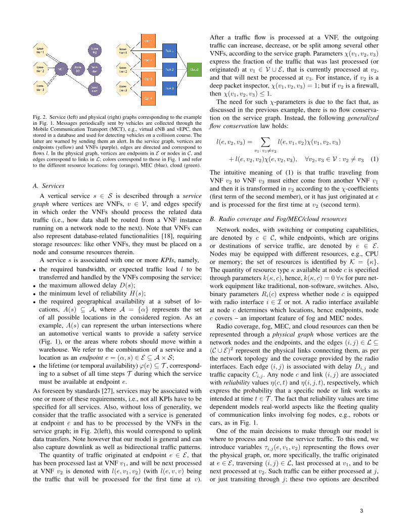
Fig. 2. Service (left) and physical (right) graphs corresponding to the examplein Fig. 1. Messages periodically sent by vehicles are collected through theMobile Communication Transport (MCT), e.g., virtual eNB and vEPC, thenstored in a database and used for detecting vehicles on a collision course. Thelatter are warned by sending them an alert. In the service graph, vertices areendpoints (yellow) and VNFs (purple), edges are directed and correspond toflows l. In the physical graph, vertices are endpoints in E or nodes in C, andedges correspond to links in L; colors correspond to those in Fig. 1 and referto the different resource locations: fog (orange), MEC (blue), cloud (green).

A. Services

A vertical service s ∈ S is described through a servicegraph where vertices are VNFs, v ∈ V , and edges specifyin which order the VNFs should process the related datatraffic (i.e., how data shall be routed from a VNF instancerunning on a network node to the next). Note that VNFs canalso represent database-related functionalities [18], requiringstorage resources: like other VNFs, they must be placed on anode and consume resources therein.A service s is associated with one or more KPIs, namely,

• the required bandwidth, or expected traffic load l to betransferred and handled by the VNFs composing the service;

• the maximum allowed delay D(s);• the minimum level of reliability H(s);• the required geographical availability at a subset of lo-cations, A(s) ⊆ A, where A = {α} represents the setof all possible locations in the considered region. As anexample, A(s) can represent the urban intersections wherean automotive vertical wants to provide a safety service(Fig. 1), or the areas where robots should move within awarehouse. We refer to the combination of a service and alocation as an endpoint e = (α, s) ∈ E ⊆ A× S;

• the lifetime (or temporal availability) ϕ(e) ⊆ T , correspond-ing to a subset of all time steps T during which the servicemust be available at endpoint e.

As foreseen by standards [27], services may be associated withone or more of these requirements, i.e., not all KPIs have to bespecified for all services. Also, without loss of generality, weconsider that the traffic associated with a service is generatedat endpoint e and has to be processed by the VNFs in theservice graph; in Fig. 2(left), this would correspond to uplinkdata transfers. Note however that our model is general and canalso capture downlink as well as bidirectional traffic patterns.The quantity of traffic originated at endpoint e ∈ E , that

has been processed last at VNF v1, and will be next processedat VNF v2 is denoted with l(e, v1, v2) (with l(e, v, v) beingthe traffic that will be processed for the first time at v).

After a traffic flow is processed at a VNF, the outgoingtraffic can increase, decrease, or be split among several otherVNFs, according to the service graph. Parameters χ(v1, v2, v3)express the fraction of the traffic that was last processed (ororiginated) at v1 ∈ V ∪ E , that is currently processed at v2,and that will next be processed at v3. For instance, if v2 is adeep packet inspector, χ(v1, v2, v3) = 1; but if v2 is a firewall,then χ(v1, v2, v3) ≤ 1.

The need for such χ-parameters is due to the fact that, asdiscussed in the previous example, there is no flow conserva-tion on the service graph. Instead, the following generalizedflow conservation law holds:

l(e, v2, v3) =�

v1: v1 �=v2

l(e, v1, v2)χ(v1, v2, v3)

+ l(e, v2, v2)χ(e, v2, v3), ∀v2, v3 ∈ V : v2 �= v3 (1)

The intuitive meaning of (1) is that traffic traveling fromVNF v2 to VNF v3 must either come from another VNF v1and then it is transformed in v2 according to the χ-coefficients(first term of the second member), or it has just originated at eand is processed for the first time at v2 (second term).

B. Radio coverage and Fog/MEC/cloud resources

Network nodes, with switching or computing capabilities,are denoted by c ∈ C, while endpoints, which are originsor destinations of service traffic, are denoted by e ∈ E .Nodes may be equipped with different resources, e.g., CPUor memory; the set of resources is identified by K = {κ}.The quantity of resource type κ available at node c is specifiedthrough parameters k(κ, c), hence, k(κ, c) = 0 ∀κ for pure net-work equipment like traditional, non-software, switches. Also,binary parameters Ri(c) express whether node c is equippedwith radio interface i ∈ I or not. A radio interface availableat node c determines which locations, hence endpoints, nodec covers – an important feature of fog and MEC nodes.Radio coverage, fog, MEC, and cloud resources can then be

represented through a physical graph whose vertices are thenetwork nodes and the endpoints, and the edges (i, j) ∈ L ⊆(C ∪ E)2 represent the physical links connecting them, as perthe network topology and the coverage provided by the radiointerfaces. Each edge (i, j) is associated with delay Di,j andtraffic capacity Ci,j . Any node c and link (i, j) are associatedwith reliability values η(c, t) and η(i, j, t), respectively, whichexpress the probability that a specific node or link works asintended at time t ∈ T . The fact that reliability values are timedependent models real-world aspects like the fleeting qualityof communication links involving fog nodes, e.g., robots orcars, as in Fig. 1.One of the main decisions to make through our model is

where to process and route the service traffic. To this end, weintroduce variables τi,j(e, v1, v2) representing the flows overthe physical graph, or, more specifically, the traffic originatedat e ∈ E , traversing (i, j) ∈ L, last processed at v1, and to benext processed at v2. Such traffic can be either processed at j,or just transiting through j; these two options are described

3

by the two real variables pi,j(e, v1, v2) and ti,j(e, v1, v2) andby imposing: τi,c(e, v1, v2) = pi,c(e, v1, v2) + ti,c(e, v1, v2).Furthermore, the traffic going out of c must be equal to thesum of that transiting through c and that just processed at c:

�

(c,h)∈Lτc,h(e, v2, v3)=

�

(i,c)∈L

�ti,c(e, v2, v3)+pi,c(e, v2, v2)·

χ(e, v2, v3) +�

v1∈Vpi,c(e, v1, v2)χ(v1, v2, v3)

�. (2)

Finally, each physical link (i, j) cannot carry more traffic thanits capacity, i.e.,

�e

�v1,v2

τi,j(e, v1, v2) ≤ Ci,j .

C. Deploying VNFs and assigning resources

A node can process traffic of a VNF if it hosts an instance ofthat VNF; this is modeled through binary variables ρ(v, c) ∈{0, 1}, expressing whether VNF v is deployed at node c.Variables ac(e, v,κ), instead, express the quantity of resourcesof type κ that are assigned to the instance of VNF v deployedat node c and used for traffic generated at endpoint e. Suchquantities cannot exceed the node capabilities, i.e., for any cand κ,

�e∈E

�v∈V ac(e, v,κ) ≤ k(κ, c).

Importantly, for any κ ∈ K, the quantity of traffic pro-cessed by v at node c cannot exceed the ratio between thequantity ac(e, v,κ) of resource type κ assigned to the VNF,and the quantity rκ(v) of resource type k needed by VNF vto process one unit of traffic:

�

(i,c)∈L

�

e∈E

�

v1∈Vpi,c(e, v1, v2) ≤

ac(e, v,κ)

rκ(v2)∀κ ∈ K . (3)

Also, node c’s resources can be assigned to a VNF v onlyif the latter is deployed therein: ac(e, v,κ) ≤ ρ(v, c)k(κ, c),for any c, κ, and v. These conditions imply that no traffic isprocessed at a node where no instance of a VNF is deployed.Last, we ensure that VNFs are placed only at nodes where

all the needed radio interface(s) are available, e.g., an MCTmay work only at nodes equipped with specific radio inter-faces. Thus, for any node c, interface i, and VNF v, we have:ρ(v, c)ri(v) ≤ Ri(c), where ri(v) ∈ {0, 1} are parametersspecifying whether interface i is needed by VNF v, and Ri(c)specifies whether such an interface is available at c.Matching service and physical flows. Since our system

model includes two graphs, we must ensure that service flows land physical flows τ match. To this end, we impose that theflow incoming the first VNF of a service graph correspondsto one or more traffic flows on the physical graph:

l(e, v, v) =�

(e,c)∈Lτe,c(e, v, v), ∀e ∈ E , v ∈ V. (4)

Once (4) is met, then (1) and (2) ensure that the traffic onsubsequent links is processed as specified by the χ-parameters.

IV. PROBLEM FORMULATION

In this section, we formalize the problem of creating end-to-end network slices that meet all the required KPI targets(Sec. IV-A) while minimizing the total cost (Sec. IV-B). Theproblem complexity is then discussed in Sec. IV-C.

A. Meeting service KPIs

To handle more easily the service KPIs, we define a string,w ∈ Wc, over the physical graph as a sequence of physicallinks traversed by a flow, with the first item of the string beingan endpoint. Similarly to [28], the possible strings can be pre-computed and stored for later usage.Since a service flow can be split across different strings, we

define f(e, v1, v2, w) as the fraction of service flow l(e, v1, v2)traversing string w. Clearly, such fractions must sum to 1.We also introduce string-wise equivalents to τi,j(e, v1, v2),ti,j(e, v1, v2), and pi,j(e, v1, v2). Specifically, τi,j(e, v1, v2, w)represents the traffic of service flow l(e, v1, v2) traversing link(i, j) on its journey through string w ∈ W , and then imposeτi,j(e, v1, v2) =

�w∈W τi,j(e, v1, v2, w). Similar definitions

and conditions hold for ti,j(e, v1, v2, w) and pi,j(e, v1, v2, w).Furthermore, the fraction of service flow over a certain

string w must match the physical traffic on the correspondinglinks, i.e., for all endpoints, VNFs v1 and v2, links, and strings,we have: f(e, v1, v2, w)l(e, v1, v2) = τi,j(e, v1, v2)1w(i,j),where 1w(i,j) denotes that link (i, j) ∈ L belongs to w.

1) Service latency: it has two components: network delaydue to traffic traversing links and switches, and processingtimes at the nodes hosting VNF instances. Given endpoint e,the average network delay can be computed as the weightedsum of the delays associated with the individual strings takenby the traffic originated at e:

dnet(e) =�

w∈W

�

v1,v2∈Vf(e, v1, v2, w)

�

(i,j)∈w

Di,j . (5)

As for the processing time, let fc(e, v1, v2) be the fraction ofthe service traffic flow l(e, v1, v2) processed at the instance ofVNF v2 located at node c. Then the quantity of traffic λc(e, v2)originating at e and processed at the instance of v2 in c is:

λc(e, v2) =�

v1∈Vfc(e, v1, v2)l(e, v1, v2).

Note that such traffic may come from different physical links.Next, we model VNF instances as M/M/1-PS queues (see,

e.g., [13]); the choice of the processor sharing (PS) policyclosely emulates the behavior of a multi-threaded applica-tion running on a virtual machine. Hence, the total pro-cessing time at the instance of v2 deployed at node c is:1/(ac(e, v2, cpu)−rcpu(v2)λc(e, v2)). Summing over all flows,the total processing delay incurred by traffic originating at ecan be written as:

dproc(e)=�

v1,v2∈V,c∈Cfc(e, v1, v2)

1

ac(e, v2, cpu)− rcpu(v2)λc(e, v2).

(6)Combining the above equation with (5), and recalling thatD(s) is the maximum target delay for service s, the servicelatency constraint for its endpoints can be stated as:

dnet(e) + dproc(e) ≤ D(s), ∀e ∈ E .Finally, note that the relationship between assigned CPU and

processing time in the expression of dproc(e) also means that

4

the CPU has a different role from the other types of resources.Indeed, for resources other than CPU, we can assign to eachVNF instance exactly the amount needed to honor (3), as agreater amount would yield no benefit. With CPU, instead,there is an additional degree of freedom we can play with:assigning more CPU results in shorter processing times, buthigher costs.2) Service geographical availability: by service availability

requirements, all locations in A(s) ⊆ A must be covered byservice s. In other words, for all endpoints e = (α, s) : α ∈A(s), there must be a link (e, c) on the physical graph to anode c that is equipped with a radio interface covering α andthat runs (or it is connected to another node running) the firstVNF of the service graph.3) Service reliability and temporal availability: the relia-

bility of a string can be computed as the product between thereliability values of all links and nodes belonging to it. We cantherefore ensure that the reliability H(s) required for services is honored, by considering a weighted sum of the per-stringreliability values. In symbols, ∀e ∈ E , t ∈ ϕ(e),

�

v1,v2∈V

�

w∈Wf(e, v1, v2, w)

�

(i,j)∈w

η(j, t)η(i, j, t) ≥ H(s) .

Note that imposing the above constraint for every time instantduring the service lifetime also ensures that the target temporalavailability is met.

B. Objective

As mentioned in Sec. I, cost is one of the main concernsrelated to service virtualization and network slicing. Such costmainly comes from using network and computation resources.To model this issue, we define:

• a fixed cost cc(v), due to the creation at node c of a VNFinstance v; this cost is null if an existing VNF instance canbe reused;

• a cost cc(κ), incurred when using a unit resource κ at node c;• a cost ci,j , incurred when one unit traffic traverses link (i, j).

Then, upon receiving a request to deploy a service instances, we formulate the following cost-minimization problem:

min�

c

�

v

�cc(v) +

�

e

�

κ

cc(κ)ac(e, v,κ)

�

+�

(i,j)

�

e

�

v1,v2

ci,jτi,j(e, v1, v2)

subject to the constraints reported in Secs. III-A–IV-A.We recall that the endpoints e to consider depend on

the service and on its geographic availability requirements,while the VNFs are those specified by the service graph.Furthermore, a solution to the above problem will always optfor reusing an existing instance of a VNF, whenever possible,as this would nullify the instantiation cost cc(v).

C. Nature and complexity of the problem

The problem of jointly making VNF placement and datarouting decisions is notoriously hard; indeed, simpler versionsthereof (considering one KPI only) have been proven to beNP-hard via reductions from the generalized assignment [13],[14] and set covering [4] problems. Thus, directly solving theabove problem is impractical for all but very small instances.We also observe that our problem can be seen as a more

complex version of a multi-constrained path (MCP) problem,where the cost (hence, the weight of the edges in the MCPgraph) changes at every hop. Although known solutions to theMCP problem, e.g., [29], are not applicable, such a similaritymotivates us to propose an effective and efficient heuristic,called OKpi, for which we prove that:• it provides high-quality VNF placement and data routingdecisions, whose feasibility is guaranteed;

• such decisions are made in polynomial time;• under mild homogeneity assumptions, decisions are optimal;• in the general case, they can be arbitrarily close to theoptimum.

V. THE OKPI SOLUTION

Our solution includes three main steps. First, by leveragingthe physical graph, we create a decision graph �G = ( �N, �E),summarizing the service deployment decisions that can bemade and their effect on the KPIs (Sec. V-A). Then wetranslate this graph into an expanded graph, and use thelatter, along with the service graph in Sec. III-A, to identify aset of feasible decisions as well as to select, among them,the lowest-cost one (Secs. V-B and V-C). For presentationclarity, we present OKpi in the case where the service graphis a chain starting from an endpoint e and including NVNFs v1 . . . vN , and only one instance of each VNF can beplaced. As discussed in Sec. V-D, both limitations can bedropped: OKpi works with arbitrary service graphs requiringany number of instances of each VNF.

A. The decision graph

Given the physical graph modeling the service endpointsand the fog, MEC, and cloud resources, we build the deci-sion graph �G with the aim to represent the possible servicedeployment decisions and their effects on the service KPIs.As a preliminary step, we consider the computation-capable

nodes in the physical graph (hence, a subset of C), and for eachof them we create (|V| − 1) replicas. Consistently, we createauxiliary edges (i) connecting each node c and its replicas ina chain fashion, and assign them zero delay, infinite capacity,and reliability 1, and (ii) connecting any replica of c withany computing node d, for which a link (c, d) ∈ L exists.Crucially, introducing node replicas enables us to account forthe possibility to deploy multiple VNFs at the same nodewithout introducing self-loops in the decision graph. Indeed,as it will be more clear later, given that a VNF is placed inc, each replica thereof represents the possibility to deploy thenext VNF again in c.Let then �G = ( �N, �E) be the decision graph where:

5

• �N includes the endpoints in E , and the computation-capablenodes in the physical graph as well as their replicas;

• �E is the set of (i) the aforementioned auxiliary links, and(ii) the virtual links (i.e., single physical links or sequencesthereof) connecting the vertices in �N .

Every edge (n1, n2) in �E representing a virtual link has thefollowing properties:

• its capacity �Cn1,n2is set to the minimum of the individual

capacities of the physical links composing the virtual link;• its delay �Dn1,n2 is set to the sum of the individual delaysof the physical links composing the virtual link;

• its reliability �ηn1,n2is set to the product of the reliability

values of physical links and nodes (both computation andpure-routing capable) included in the virtual link.

We stress that, when some services are already active in thenetwork, we build the decision graph considering the residualcapabilities of physical links and nodes, i.e., those not assignedto already-running services. Similarly, in case of virtual linkssharing the same physical links, their capacity is updated astraffic is allocated to the physical links.

B. The expanded graph: finding decisions honoring availabil-ity and additive KPIs

Given the decision graph �G, our first purpose is to identify aset of feasible service deployment decisions that are consistentwith the target KPIs. To this end, as a preliminary step,we ensure to meet the geographical and temporal availabilityrequirements by pruning from �G the vertices and edges thatdo not satisfy such constraints.Then, for the additive KPIs, we proceed as follows. To

any edge (n1, n2) in the decision graph, we assign a multi-dimensional weight w(n1, n2), defined as:

w(n1, n2) =

��Dn1,n2

D(s),log �ηn1,n2

logH(s)

�. (7)

The intuition behind (7) is that the weight of edge (n1, n2)corresponds to the fraction of the target delay and reliabilitythat will be “consumed” by taking that edge, i.e., by deployinga VNF at n1 and the subsequent one at n2. We stress thatusing logarithms in the second term of the weight allowsus to translate a multiplicative performance index (namely,reliability) into an additive one3.Next, we take an approach inspired by [29] and build

a multi-dimensional, expanded graph. Specifically, given apositive integer value of resolution γ:

1) for each vertex n in the decision graph, create (γ + 1)2

vertices4 n0,0, n0,1 . . . , n0,γ . . . , nγ,γ ;2) for every edge (n1, n2) ∈ �E with capacity �Cn1,n2

greater or equal to the amount of traffic to process,

3It is easy to see that �ηn1,n2�ηn2,n3 ≥ H(s) translates intolog �ηn1,n2logH(s)

+log �ηn2,n3logH(s)

≤ 1.4The exponent 2 corresponds to the number of additive KPIs.

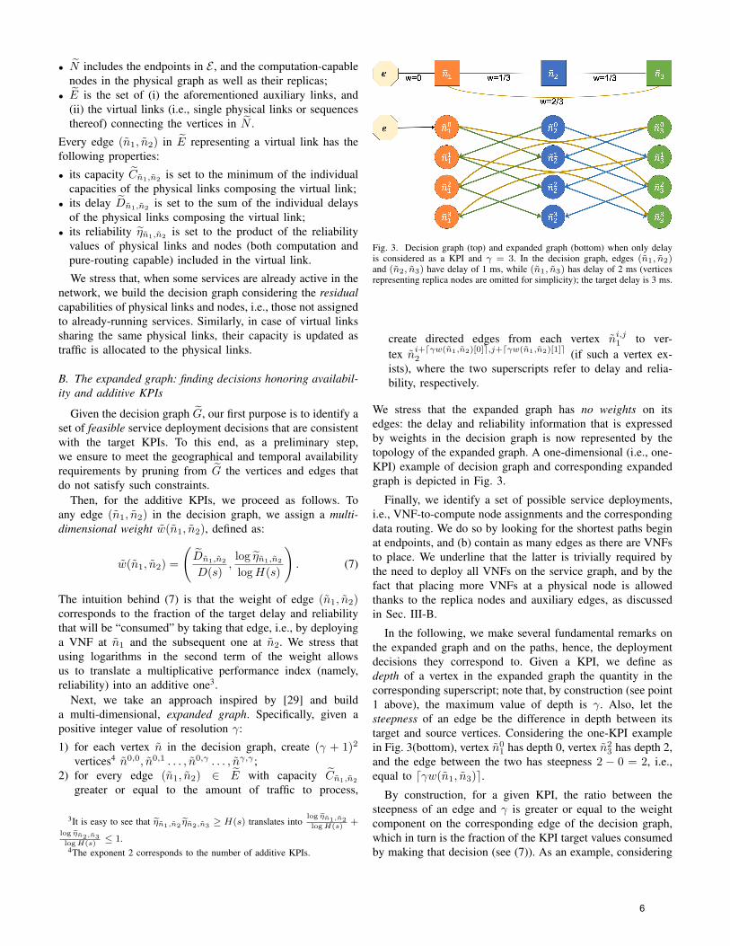
Fig. 3. Decision graph (top) and expanded graph (bottom) when only delayis considered as a KPI and γ = 3. In the decision graph, edges (n1, n2)and (n2, n3) have delay of 1 ms, while (n1, n3) has delay of 2 ms (verticesrepresenting replica nodes are omitted for simplicity); the target delay is 3 ms.

create directed edges from each vertex ni,j1 to ver-

tex ni+�γw(n1,n2)[0]�,j+�γw(n1,n2)[1]�2 (if such a vertex ex-

ists), where the two superscripts refer to delay and relia-bility, respectively.

We stress that the expanded graph has no weights on itsedges: the delay and reliability information that is expressedby weights in the decision graph is now represented by thetopology of the expanded graph. A one-dimensional (i.e., one-KPI) example of decision graph and corresponding expandedgraph is depicted in Fig. 3.

Finally, we identify a set of possible service deployments,i.e., VNF-to-compute node assignments and the correspondingdata routing. We do so by looking for the shortest paths beginat endpoints, and (b) contain as many edges as there are VNFsto place. We underline that the latter is trivially required bythe need to deploy all VNFs on the service graph, and by thefact that placing more VNFs at a physical node is allowedthanks to the replica nodes and auxiliary edges, as discussedin Sec. III-B.

In the following, we make several fundamental remarks onthe expanded graph and on the paths, hence, the deploymentdecisions they correspond to. Given a KPI, we define asdepth of a vertex in the expanded graph the quantity in thecorresponding superscript; note that, by construction (see point1 above), the maximum value of depth is γ. Also, let thesteepness of an edge be the difference in depth between itstarget and source vertices. Considering the one-KPI examplein Fig. 3(bottom), vertex n0

1 has depth 0, vertex n23 has depth 2,

and the edge between the two has steepness 2 − 0 = 2, i.e.,equal to �γw(n1, n3)�.By construction, for a given KPI, the ratio between the

steepness of an edge and γ is greater or equal to the weightcomponent on the corresponding edge of the decision graph,which in turn is the fraction of the KPI target values consumedby making that decision (see (7)). As an example, considering

6

edge (n01, n

23) in Fig. 3(bottom), we have:

steepnessγ

=2

3≥ w(n0

1, n23) =

Dn1,n3

D(s)=

2

3. (8)

The observations above allow us to state a very relevantproperty of the decisions corresponding to the paths on theexpanded graph.

Lemma 1. The decisions corresponding to any path on theexpanded graph honor all additive KPIs.

Proof: By definition, the depth of a vertex correspondsto the total steepness of the path required to reach it fromendpoint e. Given that the maximum depth in the expandedgraph is γ, there is no path with total steepness5 greaterthan γ. Thanks to the relation between weight and KPI targets(exemplified in (8)), this implies that, given a path on theexpanded graph, the sum of the weights of the correspondingedges in the decision graph cannot exceed 1, i.e., the corre-sponding decisions honor additive KPIs (including, thanks tothe logarithmic weights, reliability).Importantly, the smaller the resolution γ, the fewer the

possible values of depth and steepness in the expanded graph,the fewer the levels of consumption of the KPI target valueswe are able to distinguish, which corresponds to introducingan error, akin to quantization. Indeed, γ+1 can be seen as thenumber of quantization levels6 we admit: in the extreme caseof γ = 1, all edges would have a steepness of 1, which alsocorresponds to exhausting the whole KPI target in one hop.Such a quantization error may lead to discarding some feasiblesolutions, and thus, in the most general case, may jeopardizethe optimality of OKpi. However, two important facts standout: (i) even enumerating all feasible paths in the decisiongraph is NP-hard, as proven in [29], hence, quantization isnecessary; (ii) by increasing γ, OKpi can get arbitrarily closeto the optimum (at the price of higher complexity).Finally, we remark that all paths on the expanded graph

honor additive KPIs constraints, with the possible exceptionof delay. Indeed, unlike other KPIs, whether or not the delaytarget is violated depends not only on the network latency,hence, the VNF placement, but also on the processing time,i.e., the quantity ac(e, v, cpu) of CPU assigned to each VNF,which in turn impacts the deployment cost. We can accountfor this important aspect thanks to the M/M/1-PS model usedfor (6). In particular, below we show how to determine, givena possible deployment, whether there is a CPU assignmentconsistent with the target delay, and the cost thereof.

C. Minimizing the cost

We now need (i) for every path found in Sec. V-B, toidentify the minimum-cost CPU assignment, i.e., the optimalvalues of the ac(e, v, cpu) variables – if such an assignmentexists –, and (ii) to determine the path that minimizes theoverall cost.

5The steepness of a path should be not confused with the length of a path.6Using logarithms for reliability values, which are all typically very close

to 1, is akin to performing adaptive quantization.

To this end, for each path (hence, for a fixed e and forVNFs v1 . . . vN to be deployed at computing nodes n1 . . . nN ,respectively), we solve the following problem:

min�

n,v

an(e, v, cpu)cn(cpu) s.t. (9)

�

n1,n2

�Dn1,n2+

1

an2(e, v2, cpu)−rcpu(v2)λn2

(e, v2)

�≤D(s).

If the problem above is infeasible for a given path, then thatpath (and the corresponding decisions) is incompatible withthe delay target KPI and must be discarded.Once the problem in (9) is solved for all paths identified

in the expanded graph, we compute the total cost associatedwith each path (including all components defined in Sec. IV-B)and select and enact the lowest-cost deployment, thus fulfillingOKpi’s purpose. Importantly, the problem is convex, hence, itcan be efficiently solved in polynomial time [30]. The proofsimply follows from observing that the objective in (9) is linearand the second derivatives of the delay constraint are positivein the decision variables, hence, the constraint itself is convex.

D. General scenarios

We now show how OKpi tackles arbitrary scenarios.1) Arbitrary service graphs: If the service graph is more

complex than a chain, as in Fig. 2(left), we can proceed by (i)decomposing the graph into a set of chains (e.g., one in uplink,from the MCT to the DB, and one in downlink, from thedetector back to the MCT). OKpi is then applied subsequentlyto each chain, and the deployment decisions are cascaded.The case where multiple endpoints have to be covered, as inFig. 2(left), is handled in the same way.2) Multiple VNF instances: If the problem described in

Sec. V-C is infeasible for all possible paths found in Sec. V-B,a possible reason could be the need to split the processingburden across multiple instances of the same VNF. This caseis handled by first identifying the bottleneck VNF, i.e., takingthe longest to process the service traffic, and then increasingby one the number of instances of that VNF in the servicegraph. OKpi is then re-run on the modified service graph.

VI. OKPI ANALYSIS

In this section, we prove several properties about OKpi; westart with the most essential aspect related to its effectiveness,i.e., its ability to meet all service KPIs.

Property 1. OKpi’s decisions honor all KPI targets.

Proof: By Lemma 1, all decisions honor the additiveKPIs. Concerning delay, it is guaranteed that such a KPItarget is met, thanks to the delay constraint imposed whileperforming the CPU assignment. As noted in Sec. V-C, deci-sions resulting in an infeasible problem are discarded, hence,the selected decision honors the delay target. Finally, theavailability constraints are satisfied through the initial selectionof the vertices of the decision graph (see Sec. V-B).Next, we address the computational complexity of OKpi.

7

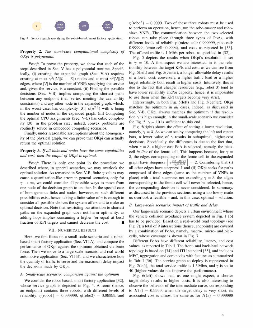
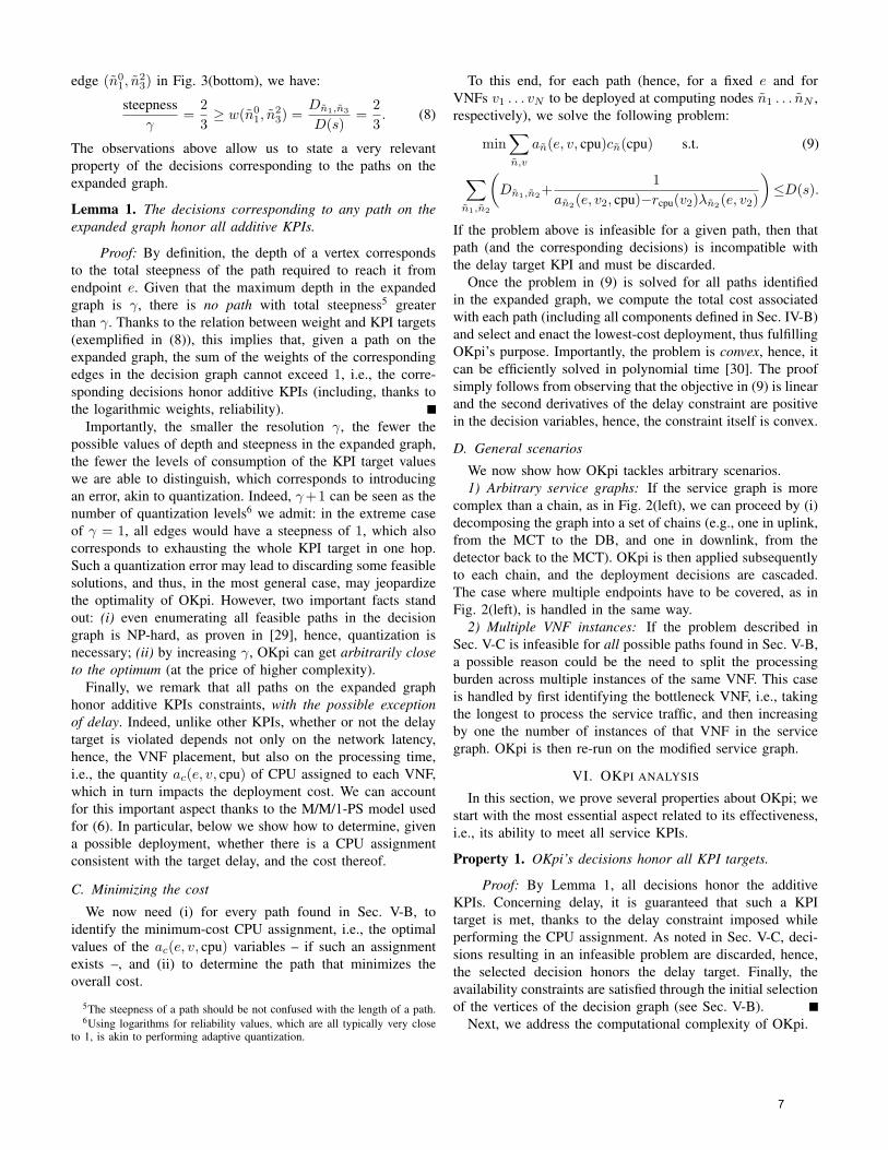
Fig. 4. Service graph specifying the robot-based, smart factory application.

Property 2. The worst-case computational complexity ofOKpi is polynomial.

Proof: To prove the property, we show that each of thesteps described in Sec. V has a polynomial runtime. Specif-ically, (i) creating the expanded graph (Sec. V-A) requirescreating at most γ2(|V||C|+ |E|) nodes and at most γ2|V||L|edges, where |V| is the number of VNFs specifying the serviceand, given the service, is a constant. (ii) Finding the possibledecisions (Sec. V-B) implies computing the shortest pathsbetween any endpoint (i.e., vertex meeting the availabilityconstraints) and any other node in the expanded graph, which,in the worst case, has complexity [31] o(n2.3) with n beingthe number of nodes in the expanded graph. (iii) Computingthe optimal CPU assignments (Sec. V-C) has cubic complex-ity [30] in the problem size; indeed, convex problems areroutinely solved in embedded computing scenarios.Finally, under reasonable assumptions about the homogene-

ity of the physical graph, we can prove that OKpi can actuallyreturn the optimal solution.

Property 3. If all links and nodes have the same capabilitiesand cost, then the output of OKpi is optimal.

Proof: There is only one point in the procedure wedescribed where, in general scenarios, we may overlook theoptimal solution. As remarked in Sec. V-B, finite γ values maycause a quantization-like error: in general scenarios, only forγ → ∞, we could consider all possible ways to move fromone node of the decision graph to another. In the special caseof homogeneous links and nodes, however, no such differentpossibilities exist, hence, taking a finite value of γ is enough toconsider all possible choices the system offers and to make anoptimal decision. Note that restricting our attention to shortestpaths on the expanded graph does not harm optimality, asadding hops implies consuming a higher (or equal at best)fraction of KPI targets and cannot decrease the cost.

VII. NUMERICAL RESULTS

Here, we first focus on a small-scale scenario and a robot-based smart factory application (Sec. VII-A), and compare theperformance of OKpi against the optimum obtained via bruteforce. Then we move to a large-scale scenario and real-worldautomotive application (Sec. VII-B), and we characterize howthe quantity of traffic to serve and the maximum delay impactthe decisions made by OKpi.

A. Small-scale scenario: comparison against the optimum

We consider the robot-based, smart factory application [32],whose service graph is depicted in Fig. 4. A room (hence,an endpoint) contains three robots, with different levels ofreliability: η(robo1) = 0.999999, η(robo2) = 0.99999, and

η(robo3) = 0.9999. Two of these three robots must be usedto perform an operation, hence, run the robo-master and robo-slave VNFs. The communication between the two selectedrobots can take place through three types of PoAs, withdifferent levels of reliability (micro-cell: 0.999999, pico-cell:0.99999, femto-cell: 0.9994), and costs as reported in [33].The offered traffic is 1 Mb/s per robot, as specified in [32].Fig. 5 depicts the results when OKpi’s resolution is set

to γ = 10. A first aspect we are interested in is the rela-tionship between the target KPIs and cost: as we can see fromFig. 5(left) and Fig. 5(center), a longer allowable delay resultsin a lower cost; conversely, a higher traffic load or a highertarget reliability both result in higher costs. Intuitively, this isdue to the fact that cheaper resources (e.g., robot 3) tend tohave lower reliability and/or capacity, hence, it is impossibleto use them when the KPI targets become very strict.Interestingly, in both Fig. 5(left) and Fig. 5(center), OKpi

matches the optimum in all cases. Indeed, as discussed inSec. V-B, OKpi always matches the optimum if the resolu-tion γ is high enough; in the small-scale scenario we considerfor Fig. 5, γ = 10 is sufficient to this end.Fig. 5(right) shows the effect of setting a lower resolution,

namely, γ = 3. As we can see by comparing the left and centerbars, a lower value of γ results in suboptimal, higher-costdecisions. Specifically, the difference is due to the fact that,when γ = 3, a higher-cost PoA is selected, namely, the pico-cell in lieu of the femto-cell. This happens because, for γ =3, the edges corresponding to the femto-cell in the expandedgraph have steepness

�γ log 0.9994

log 0.999

�= 2. Considering that (i)

all other edges have steepness 1 and (ii) OKpi seeks for pathscomposed of three edges (same as the number of VNFs toplace) with a total steepness not exceeding γ = 3, the edgescorresponding to the femto-cell will never be selected, hence,the corresponding decision is never considered. In summary,as discussed in the previous sections, using a too-low γ madeus overlook a feasible – and, in this case, optimal – solution.

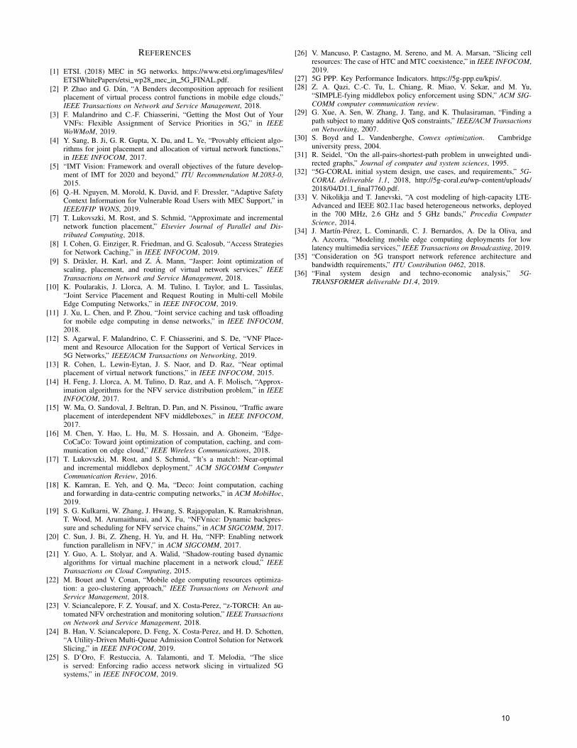
B. Large-scale scenario: impact of traffic and delay

Our large-scale scenario depicts a urban environment wherethe vehicle collision avoidance system depicted in Fig. 1 [6]has to be provided. Based on a real-world road topology (seeFig. 7), a total of 9 intersections (hence, endpoints) are coveredby a combination of PoAs, namely, macro-, micro- and pico-cells, whose coverage is shown in Fig. 7.Different PoAs have different reliability, latency, and cost

values, as reported in Tab. I. The front- and back-haul networktopology is based on [34] and ITU standard [35], and includesMEC, aggregation and core nodes with features as summarizedin Tab. I [36]. The service graph to deploy is represented inFig. 2(left), the total service traffic is 1.5Mb/s, and γ is set to40 (higher values do not improve the performance).Fig. 6(left) shows that, as one might expect, a shorter

target delay results in higher costs. It is also interesting toobserve the behavior of the intermediate curve, correspondingto H(s) = 0.9999: when the target delay is very short, itsassociated cost is almost the same as for H(s) = 0.999999

8

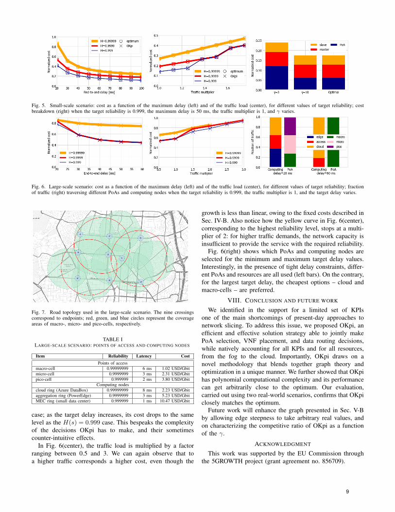
Fig. 5. Small-scale scenario: cost as a function of the maximum delay (left) and of the traffic load (center), for different values of target reliability; costbreakdown (right) when the target reliability is 0.999, the maximum delay is 50 ms, the traffic multiplier is 1, and γ varies.

Fig. 6. Large-scale scenario: cost as a function of the maximum delay (left) and of the traffic load (center), for different values of target reliability; fractionof traffic (right) traversing different PoAs and computing nodes when the target reliability is 0.999, the traffic multiplier is 1, and the target delay varies.

Fig. 7. Road topology used in the large-scale scenario. The nine crossingscorrespond to endpoints; red, green, and blue circles represent the coverageareas of macro-, micro- and pico-cells, respectively.

TABLE ILARGE-SCALE SCENARIO: POINTS OF ACCESS AND COMPUTING NODES

Item Reliability Latency CostPoints of access

macro-cell 0.99999999 6 ms 1.02 USD/Gbitmicro-cell 0.9999999 3 ms 2.31 USD/Gbitpico-cell 0.999999 2 ms 3.80 USD/Gbit

Computing nodescloud ring (Azure DataBox) 0.99999999 8 ms 2.23 USD/Gbitaggregation ring (PowerEdge) 0.9999999 3 ms 5.23 USD/GbitMEC ring (small data center) 0.999999 1 ms 10.47 USD/Gbit

case; as the target delay increases, its cost drops to the samelevel as the H(s) = 0.999 case. This bespeaks the complexityof the decisions OKpi has to make, and their sometimescounter-intuitive effects.In Fig. 6(center), the traffic load is multiplied by a factor

ranging between 0.5 and 3. We can again observe that toa higher traffic corresponds a higher cost, even though the

growth is less than linear, owing to the fixed costs described inSec. IV-B. Also notice how the yellow curve in Fig. 6(center),corresponding to the highest reliability level, stops at a multi-plier of 2: for higher traffic demands, the network capacity isinsufficient to provide the service with the required reliability.Fig. 6(right) shows which PoAs and computing nodes are

selected for the minimum and maximum target delay values.Interestingly, in the presence of tight delay constraints, differ-ent PoAs and resources are all used (left bars). On the contrary,for the largest target delay, the cheapest options – cloud andmacro-cells – are preferred.

VIII. CONCLUSION AND FUTURE WORK

We identified in the support for a limited set of KPIsone of the main shortcomings of present-day approaches tonetwork slicing. To address this issue, we proposed OKpi, anefficient and effective solution strategy able to jointly makePoA selection, VNF placement, and data routing decisions,while natively accounting for all KPIs and for all resources,from the fog to the cloud. Importantly, OKpi draws on anovel methodology that blends together graph theory andoptimization in a unique manner. We further showed that OKpihas polynomial computational complexity and its performancecan get arbitrarily close to the optimum. Our evaluation,carried out using two real-world scenarios, confirms that OKpiclosely matches the optimum.Future work will enhance the graph presented in Sec. V-B

by allowing edge steepness to take arbitrary real values, andon characterizing the competitive ratio of OKpi as a functionof the γ.

ACKNOWLEDGMENT

This work was supported by the EU Commission throughthe 5GROWTH project (grant agreement no. 856709).

9

REFERENCES

[1] ETSI. (2018) MEC in 5G networks. https://www.etsi.org/images/files/ETSIWhitePapers/etsi wp28 mec in 5G FINAL.pdf.

[2] P. Zhao and G. Dan, “A Benders decomposition approach for resilientplacement of virtual process control functions in mobile edge clouds,”IEEE Transactions on Network and Service Management, 2018.

[3] F. Malandrino and C.-F. Chiasserini, “Getting the Most Out of YourVNFs: Flexible Assignment of Service Priorities in 5G,” in IEEEWoWMoM, 2019.

[4] Y. Sang, B. Ji, G. R. Gupta, X. Du, and L. Ye, “Provably efficient algo-rithms for joint placement and allocation of virtual network functions,”in IEEE INFOCOM, 2017.

[5] “IMT Vision: Framework and overall objectives of the future develop-ment of IMT for 2020 and beyond,” ITU Recommendation M.2083-0,2015.

[6] Q.-H. Nguyen, M. Morold, K. David, and F. Dressler, “Adaptive SafetyContext Information for Vulnerable Road Users with MEC Support,” inIEEE/IFIP WONS, 2019.

[7] T. Lukovszki, M. Rost, and S. Schmid, “Approximate and incrementalnetwork function placement,” Elsevier Journal of Parallel and Dis-tributed Computing, 2018.

[8] I. Cohen, G. Einziger, R. Friedman, and G. Scalosub, “Access Strategiesfor Network Caching,” in IEEE INFOCOM, 2019.

[9] S. Draxler, H. Karl, and Z. A. Mann, “Jasper: Joint optimization ofscaling, placement, and routing of virtual network services,” IEEETransactions on Network and Service Management, 2018.

[10] K. Poularakis, J. Llorca, A. M. Tulino, I. Taylor, and L. Tassiulas,“Joint Service Placement and Request Routing in Multi-cell MobileEdge Computing Networks,” in IEEE INFOCOM, 2019.

[11] J. Xu, L. Chen, and P. Zhou, “Joint service caching and task offloadingfor mobile edge computing in dense networks,” in IEEE INFOCOM,2018.

[12] S. Agarwal, F. Malandrino, C. F. Chiasserini, and S. De, “VNF Place-ment and Resource Allocation for the Support of Vertical Services in5G Networks,” IEEE/ACM Transactions on Networking, 2019.

[13] R. Cohen, L. Lewin-Eytan, J. S. Naor, and D. Raz, “Near optimalplacement of virtual network functions,” in IEEE INFOCOM, 2015.

[14] H. Feng, J. Llorca, A. M. Tulino, D. Raz, and A. F. Molisch, “Approx-imation algorithms for the NFV service distribution problem,” in IEEEINFOCOM, 2017.

[15] W. Ma, O. Sandoval, J. Beltran, D. Pan, and N. Pissinou, “Traffic awareplacement of interdependent NFV middleboxes,” in IEEE INFOCOM,2017.

[16] M. Chen, Y. Hao, L. Hu, M. S. Hossain, and A. Ghoneim, “Edge-CoCaCo: Toward joint optimization of computation, caching, and com-munication on edge cloud,” IEEE Wireless Communications, 2018.

[17] T. Lukovszki, M. Rost, and S. Schmid, “It’s a match!: Near-optimaland incremental middlebox deployment,” ACM SIGCOMM ComputerCommunication Review, 2016.

[18] K. Kamran, E. Yeh, and Q. Ma, “Deco: Joint computation, cachingand forwarding in data-centric computing networks,” in ACM MobiHoc,2019.

[19] S. G. Kulkarni, W. Zhang, J. Hwang, S. Rajagopalan, K. Ramakrishnan,T. Wood, M. Arumaithurai, and X. Fu, “NFVnice: Dynamic backpres-sure and scheduling for NFV service chains,” in ACM SIGCOMM, 2017.

[20] C. Sun, J. Bi, Z. Zheng, H. Yu, and H. Hu, “NFP: Enabling networkfunction parallelism in NFV,” in ACM SIGCOMM, 2017.

[21] Y. Guo, A. L. Stolyar, and A. Walid, “Shadow-routing based dynamicalgorithms for virtual machine placement in a network cloud,” IEEETransactions on Cloud Computing, 2015.

[22] M. Bouet and V. Conan, “Mobile edge computing resources optimiza-tion: a geo-clustering approach,” IEEE Transactions on Network andService Management, 2018.

[23] V. Sciancalepore, F. Z. Yousaf, and X. Costa-Perez, “z-TORCH: An au-tomated NFV orchestration and monitoring solution,” IEEE Transactionson Network and Service Management, 2018.

[24] B. Han, V. Sciancalepore, D. Feng, X. Costa-Perez, and H. D. Schotten,“A Utility-Driven Multi-Queue Admission Control Solution for NetworkSlicing,” in IEEE INFOCOM, 2019.

[25] S. D’Oro, F. Restuccia, A. Talamonti, and T. Melodia, “The sliceis served: Enforcing radio access network slicing in virtualized 5Gsystems,” in IEEE INFOCOM, 2019.

[26] V. Mancuso, P. Castagno, M. Sereno, and M. A. Marsan, “Slicing cellresources: The case of HTC and MTC coexistence,” in IEEE INFOCOM,2019.

[27] 5G PPP. Key Performance Indicators. https://5g-ppp.eu/kpis/.[28] Z. A. Qazi, C.-C. Tu, L. Chiang, R. Miao, V. Sekar, and M. Yu,

“SIMPLE-fying middlebox policy enforcement using SDN,” ACM SIG-COMM computer communication review.

[29] G. Xue, A. Sen, W. Zhang, J. Tang, and K. Thulasiraman, “Finding apath subject to many additive QoS constraints,” IEEE/ACM Transactionson Networking, 2007.

[30] S. Boyd and L. Vandenberghe, Convex optimization. Cambridgeuniversity press, 2004.

[31] R. Seidel, “On the all-pairs-shortest-path problem in unweighted undi-rected graphs,” Journal of computer and system sciences, 1995.

[32] “5G-CORAL initial system design, use cases, and requirements,” 5G-CORAL deliverable 1.1, 2018, http://5g-coral.eu/wp-content/uploads/2018/04/D1.1 final7760.pdf.

[33] V. Nikolikja and T. Janevski, “A cost modeling of high-capacity LTE-Advanced and IEEE 802.11ac based heterogeneous networks, deployedin the 700 MHz, 2.6 GHz and 5 GHz bands,” Procedia ComputerScience, 2014.

[34] J. Martın-Perez, L. Cominardi, C. J. Bernardos, A. De la Oliva, andA. Azcorra, “Modeling mobile edge computing deployments for lowlatency multimedia services,” IEEE Transactions on Broadcasting, 2019.

[35] “Consideration on 5G transport network reference architecture andbandwidth requirements,” ITU Contribution 0462, 2018.

[36] “Final system design and techno-economic analysis,” 5G-TRANSFORMER deliverable D1.4, 2019.

10