Int J Adv Manuf Technol (2011) 53:1129–1139DOI 10.1007/s00170-010-2906-x

ORIGINAL ARTICLE

Scheduling wafer slicing by multi-wire saw manufacturingin photovoltaic industry: a case study

Luis Guimarães · Rui Santos · Bernardo Almada-Lobo

Received: 5 April 2010 / Accepted: 16 August 2010 / Published online: 14 September 2010© Springer-Verlag London Limited 2010

Abstract Wafer slicing in photovoltaic industry ismainly done using multi-wire saw machines. The selec-tion of set of bricks (parallelepiped block of crystallinesilicon) to be sawn together poses difficult productionscheduling decisions. The objective is to maximize theutilization of the available cutting length to improvethe process throughput. We address the problem pre-senting a mathematical formulation and an algorithmthat aims to solve it in very short running times whiledelivering superior solutions. The algorithm employs areactive greedy randomized adaptive search procedurewith some enhancements. Computational experimentsproved its effectiveness and efficiency to solve real-world based problems and randomly generated in-stances. Implementation of an on-line decision systembased on this algorithm can help photovoltaic industryto reduce slicing costs making a contribution for itscompetitiveness against other sources of energy.

Keywords Multi-wire saw wafer slicing · Operationalresearch · Production scheduling · Mixed integerprogramming · Metaheuristics

1 Introduction

Photovoltaic (PV) technology generates renewable en-ergy by directly converting sunlight into electricity. PVsystems provide a quiet, clean, and safe energy offering

L. Guimarães · R. Santos · B. Almada-Lobo (B)Faculdade de Engenharia da Universidade do Porto,Porto, Portugale-mail: almada.lobo@fe.up.pt

a way to replace the use of finite fossil resources respon-sible for greenhouse gas emissions. A large variety ofapplications are available ranging from consumer prod-uct modules placed on roofs of houses or integrated ina building skin up to industrial applications and largepower stations. PV also fits well in the existing in-frastructure and offers possibilities to make intelligentmatches between electricity supply and demand.

Historically, the PV industry has enjoyed stronggrowth driven by renewable energy incentives policiesand governmental subsidy programs. The Europeanmarket evolved from 1.200 MW of cumulative installedcapacity of solar PV systems in 2000 to an impressivefigure of 9.200 MW by the end of 2007, representingin 2005 a annual market of e13 billion according toEuropean Photovoltaic Industry Association andGreenpeace [1] report.

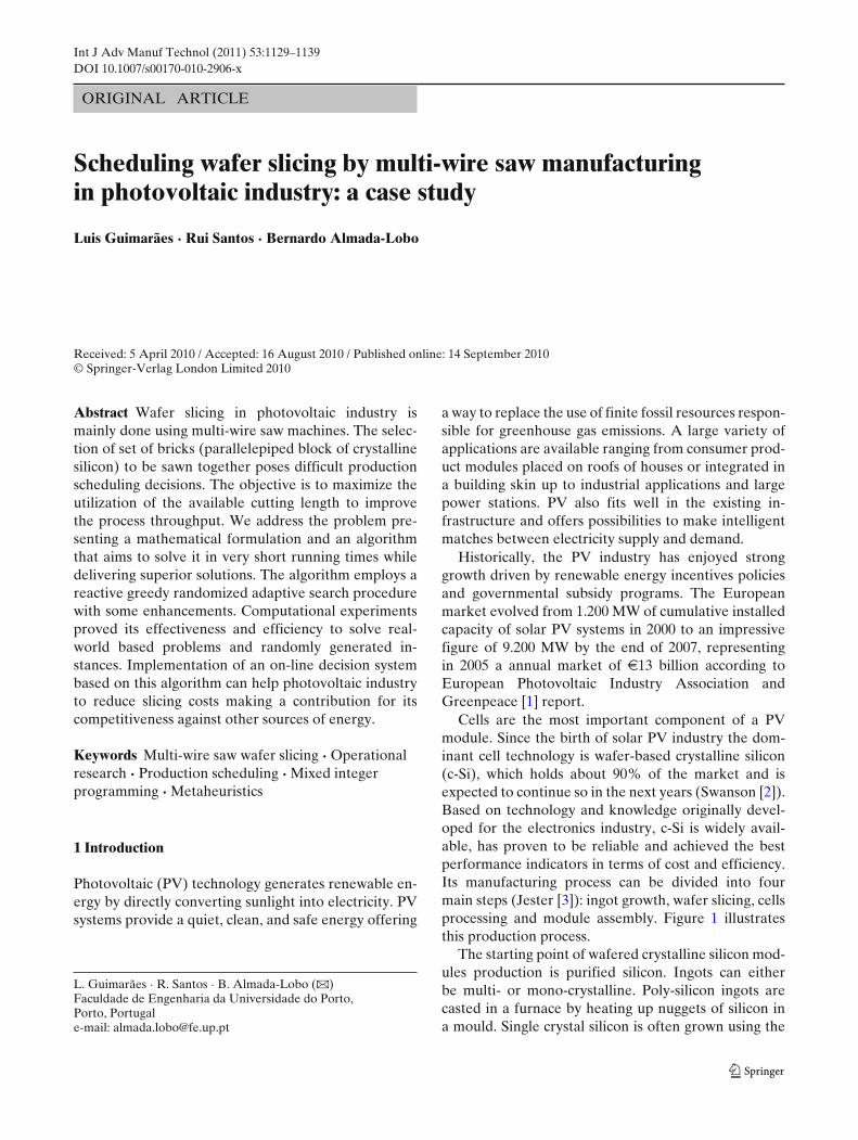
Cells are the most important component of a PVmodule. Since the birth of solar PV industry the dom-inant cell technology is wafer-based crystalline silicon(c-Si), which holds about 90% of the market and isexpected to continue so in the next years (Swanson [2]).Based on technology and knowledge originally devel-oped for the electronics industry, c-Si is widely avail-able, has proven to be reliable and achieved the bestperformance indicators in terms of cost and efficiency.Its manufacturing process can be divided into fourmain steps (Jester [3]): ingot growth, wafer slicing, cellsprocessing and module assembly. Figure 1 illustratesthis production process.

The starting point of wafered crystalline silicon mod-ules production is purified silicon. Ingots can eitherbe multi- or mono-crystalline. Poly-silicon ingots arecasted in a furnace by heating up nuggets of silicon ina mould. Single crystal silicon is often grown using the

1130 Int J Adv Manuf Technol (2011) 53:1129–1139

Fig. 1 Solar cells productionprocess

Czochralski process (Zulehner [4]) forming cylindricalingots, which need to be cropped into square shape.The ingots are then cut into bricks in the final squareprofile of the solar cell. Multi-wire slurry saws slice thebricks into wafers. After sliced wafers are separated,washed and inspected. Following the quality inspection,wafers are processed into solar cells and integrated insolar modules designed to be weather-proof packages.

Nowadays, the PV industry eagerly seeks furthercost reduction in order to become more competitivein relation to other power sources. A wide range offields such as search of efficiency, energy yield, sta-bility and lifetime, high-productivity manufacturing,in-process monitoring & control, environmental sus-tainability and applicability drive the undergoing re-search. The cost per watt (e/W) is the ultimate keymetric for assessing PV industry competitiveness and,therefore, also for wafer-based crystalline silicon tech-nology. In Cañizo et al. [5], a cost analysis of thecrystalline silicon manufacturing process and the po-tential for cost reduction are studied. Since the waferproduction is one of the most expensive steps of crys-talline silicon-based PV manufacturing flow, reducingwafer fabrication cost is critical to the goal of makingsolar energy competitive. We address high-productivemanufacturing by studying the crystalline silicon wafersslicing process in multi-wire saw machines, PV mar-ket main slicing technique. The aim is to improvethe process throughput through efficient productionscheduling. Increasing the throughput of the processmeans correctly allocate bricks to holders before pro-ceed to the sawing machine. Bricks have different

lengths while the holders represent a fix cutting length.The final objective is to maximize the usage of theavailable cutting length. Our motivation comes fromone of the biggest players worldwide that performsthis key scheduling step manually. To the best of ourknowledge, we are first to develop a solution proce-dure to solve this problem. Results obtained in pseudo-real-world instances clearly validate the suggestedalgorithm.

The remainder of the paper is organized as follows.Section 2 describes the problem in detail. A mixedinteger linear formulation is introduced in Section 3.Several solution algorithms are presented in Section 4.Experimental results are reported in Section 5 followedby concluding remarks made in Section 6.

2 Problem description

The wafer slicing process uses multi-wire saw machinesthat have a limited available cutting length. To producea cut, a single strand of wire moves from a feed reel to atake-up reel. In between, the wire goes through the en-trance side of storage system called the “carriage” andinto the rectangular arrangement of fixed shafts with re-placeable wire guides. The wire wraps around the wireguides which have hundreds of grooves. This creates amultiple net of parallel wires known as web, the totalweb length equals the available cutting length. Beforebeing fed together with an abrasive slurry in order to besliced into wafers, bricks are glued and mounted into aholder. Glueing, as it is called, is the procedure under

Int J Adv Manuf Technol (2011) 53:1129–1139 1131

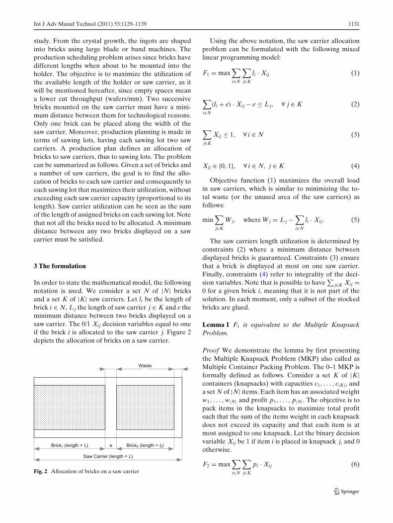
study. From the crystal growth, the ingots are shapedinto bricks using large blade or band machines. Theproduction scheduling problem arises since bricks havedifferent lengths when about to be mounted into theholder. The objective is to maximize the utilization ofthe available length of the holder or saw carrier, as itwill be mentioned hereafter, since empty spaces meana lower cut throughput (wafers/mm). Two successivebricks mounted on the saw carrier must have a mini-mum distance between them for technological reasons.Only one brick can be placed along the width of thesaw carrier. Moreover, production planning is made interms of sawing lots, having each sawing lot two sawcarriers. A production plan defines an allocation ofbricks to saw carriers, thus to sawing lots. The problemcan be summarized as follows. Given a set of bricks anda number of saw carriers, the goal is to find the allo-cation of bricks to each saw carrier and consequently toeach sawing lot that maximizes their utilization, withoutexceeding each saw carrier capacity (proportional to itslength). Saw carrier utilization can be seen as the sumof the length of assigned bricks on each sawing lot. Notethat not all the bricks need to be allocated. A minimumdistance between any two bricks displayed on a sawcarrier must be satisfied.

3 The formulation

In order to state the mathematical model, the followingnotation is used. We consider a set N of |N| bricksand a set K of |K| saw carriers. Let li be the length ofbrick i ∈ N, L j the length of saw carrier j ∈ K and e theminimum distance between two bricks displayed on asaw carrier. The 0/1 Xij decision variables equal to oneif the brick i is allocated to the saw carrier j. Figure 2depicts the allocation of bricks on a saw carrier.

\

L

1 l1 2 l2

Fig. 2 Allocation of bricks on a saw carrier

Using the above notation, the saw carrier allocationproblem can be formulated with the following mixedlinear programming model:

F1 = max∑

i∈N

∑

j∈K

li · Xij (1)

∑

i∈N

(li + e) · Xij − e ≤ L j, ∀ j ∈ K (2)

∑

j∈K

Xij ≤ 1, ∀ i ∈ N (3)

Xij ∈ {0, 1}, ∀ i ∈ N, j ∈ K (4)

Objective function (1) maximizes the overall loadin saw carriers, which is similar to minimizing the to-tal waste (or the unused area of the saw carriers) asfollows:

min∑

j∈K

W j, where W j = L j −∑

i∈N

li · Xij. (5)

The saw carriers length utilization is determined byconstraints (2) where a minimum distance betweendisplayed bricks is guaranteed. Constraints (3) ensurethat a brick is displayed at most on one saw carrier.Finally, constraints (4) refer to integrality of the deci-sion variables. Note that is possible to have

∑j∈K Xij =

0 for a given brick i, meaning that it is not part of thesolution. In each moment, only a subset of the stockedbricks are glued.

Lemma 1 F1 is equivalent to the Multiple KnapsackProblem.

Proof We demonstrate the lemma by first presentingthe Multiple Knapsack Problem (MKP) also called asMultiple Container Packing Problem. The 0–1 MKP isformally defined as follows. Consider a set K of |K|containers (knapsacks) with capacities c1, . . . , c|K|, anda set N of |N| items. Each item has an associated weightw1, . . . , w|N| and profit p1, . . . , p|N|. The objective is topack items in the knapsacks to maximize total profitsuch that the sum of the items weight in each knapsackdoes not exceed its capacity and that each item is atmost assigned to one knapsack. Let the binary decisionvariable Xij be 1 if item i is placed in knapsack j, and 0otherwise.

F2 = max∑

i∈N

∑

j∈K

pi · Xij (6)

1132 Int J Adv Manuf Technol (2011) 53:1129–1139

∑

i∈N

wi · Xij ≤ c j, ∀ j ∈ K (7)

∑

j∈K

Xij ≤ 1, ∀ i ∈ N (8)

Xij ∈ {0, 1}, ∀ i ∈ N, j ∈ K (9)

It is easy to see that F1 equals to F2, making pi = li,wi = li + e and c j = L j + e. ��

The MKP has attracted attention from theoreticiansand practicians and has enjoyed a great popularity(Martello and Toth [6]). It has a simple structure andcan be used as sub-problems of more complicated ver-sions. For instance, it can model several real-worldapplications such as vehicle/container loading (Eilonand Christofides [7]), cutting stock and capital budget.

The MKP is NP-hard in the strong sense. State-of-the-art algorithms for solving it are based onbranch-and-bound (Pisinger [8] and Fukunaga [9]).Nevertheless, exact approaches tend to fail when largedimension instances are to be solved. Some work isavailable on approximation algorithms (Caprara et al.[10] and Martello and Toth [11]). Khuri et al. [12], Raidl[13] and Fukunaga [14]) employ genetic algorithmsto solve this problem. Extended overviews on MKPcan be found in Kellerer et al. [15] and Martello andToth [6].

The purpose of this paper is to develop a fast andefficient algorithm capable of solving the aforemen-tioned problem in very short computational time whiledelivering superior solutions, making it able to beimplemented in a real-world application. Such proce-dure needs to be robust and its performance instance-independent. The output of this approach will becompared with the exact algorithm of Pisinger [8]. TheMulknap, as it is called, is an item-oriented branch-and-bound algorithm, similar to the MTM algorithm ofMartello and Toth [11]. At each node, the algorithmtries to validate the surrogate relaxed multiple knap-sack problem, which is equivalent to solve a 0–1 singleknapsack problem. An item reduction and capacitytightening procedures are also performed in each node.This algorithm has proved to be extremely powerful.For many problems, the optimal solutions found at theroot node, making it a good comparison basis for ourapproach.

4 The solution approach

The practicability and conditions of our case study werethe focus during the design options of our algorithm.

We have applied concepts derived from greedy ran-domize adaptive search procedure (GRASP). GRASPis a metaheuristic that has been applied with greatsuccess to solve combinatorial problems, see Feo andResende [16] for a general presentation. GRASP isa multi-start method, consisting in two phases: initialsolution construction and local search. The construc-tion phase iteratively builds a feasible solution oneelement at time. Since constructed solutions are likelyto be locally sub-optimal, the local search phase ex-plores their neighbourhood seeking for a local opti-mum. The overall best solution achieved is returnedas result.

At each iteration of the construction phase a setof feasible elements to be incorporated in the solu-tion under construction is evaluated according to agreedy function. The greedy function measures theincremental benefit or cost associated with the selectionof the evaluated element, leading to the creation ofthe so-called restricted candidate list (RCL) formed bythe best elements. The amount of greediness of thealgorithm can be controlled by a threshold parame-ter α ∈ [0, 1]. The best elements composing the RCLare those whose quality, assessed by the incremen-tal cost function f (e), is within the acceptance range[ fmin, fmin + α( fmax − fmin)]. A pure greedy algorithmcan be obtained setting α = 0, while defining α = 1results in a complete random construction algorithm.Afterwards, an element is probabilistic chosen fromRCL and inserted in the partial solution. The can-didates are re-evaluated to reflect the changes de-rived from the previous selections and RCL is updatedmaking the algorithm adaptive. This process allowsthe creation of solutions with different characteristicsthroughout the iterations.

The local search phase attempts to improve theconstructed solution until a local optimum is found.It replaces the current solution by a better one in itsneighbourhood. The neighbourhood structure, searchtechnique and evaluation scheme of neighbours arevery important when designing local search since theydirectly affect its effectiveness. To assure quick itera-tions, often a simple neighbourhood is chosen.

Diverse successful applications of GRASP havebeen reported such as in [17–20]. GRASP was pre-ferred due to its relatively simple structure and smallnumber of parameters to be set and tuned. In fact,it has mainly two parameters: the stopping criterionand the threshold parameter. The former is usuallydetermined by a maximum number of iterations and thelatter tends to be user-defined. Like any metaheuristic,GRASP provides a general structure and its design isproblem-specific. In the next subsections, we present a

Int J Adv Manuf Technol (2011) 53:1129–1139 1133

specialization of GRASP to deal with the saw carrierallocation problem.

4.1 Construction phase

The construction phase builds a feasible solution by al-locating the available bricks on stock saw carrier by sawcarrier until all are loaded. At each step only one sawcarrier is analysed. In preliminary tests such approachrevealed to be more efficient than that considering allsaw carriers at each iteration. Recall that i ∈ N denotesa brick and li its length, L j the length of saw carrierj ∈ K and e the minimum distance between two bricksdisplayed on a saw carrier. While constructing the ini-tial solution, we also need to define d j as the availablespace in the saw carrier j, u j as the number of assignedbricks to saw carrier j and � as the set of unassignedbricks. In each instant, the candidates correspond tothe unassigned bricks (i ∈ �) with length inferior tolmax

jn (u jn) given by:

lmaxjn (u jn) =

{d jn , if u jn = 0d jn − e , if u jn > 0

(10)

where jn denotes the current saw carrier. Let this setof “feasible” bricks be expressed as �. The greedyfunction h(i) evaluates the “feasible” bricks accordingto the remaining available space in the current underloading saw carrier jn in case brick i ∈ � is assigned.The best fit decreasing heuristic inspired the greedyfunction.

h(i) ={

d jn − li , if u jn = 0d jn − li − e , if u jn > 0

(11)

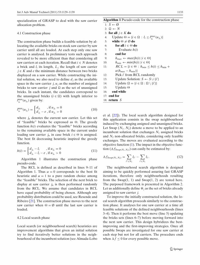
Algorithm 1 illustrates the construction phasepseudo-code.

The RCL is defined as described in lines 9–11 ofAlgorithm 1. Thus α = 0 corresponds to the best fitheuristic and α = 1 to a pure random choice amongthe “feasible” bricks. The selection of the next brick todisplay at saw carrier jn is then performed randomlyfrom the RCL. We assume that candidates in RCLhave equal probability of being chosen. Although anyprobability distribution could be used, see Resende andRibeiro [21]. The construction phase moves to the nextsaw carrier when � = Ø until the last saw carrier isloaded.

4.2 Local search phase

Local search (or neighbourhood search) heuristics areimprovement algorithms that given an initial solutiontry to find iteratively better solutions in the neigh-bourhood of the incumbent solution (see Almada-Lobo

Algorithm 1 Pseudo-code for the construction phase1: S ← Ø2: � ← N3: for all j ∈ K do4: Update � = {i ∈ � : li ≤ lmax

jn (u jn)}5: while � �= Ø do6: for all i ∈ � do7: Evaluate h(i)8: end for9: hmax ← max{h(i) | i ∈ �}

10: hmin ← min{h(i) | i ∈ �}11: RCL = {i ∈ � : hmin ≤ h(i) ≤ hmin +

α(hmax − hmin)}12: Pick i′ from RCL randomly13: Update Solution: S ← S ∪ {i′}14: Update � = {i ∈ � : � \ {i′}}15: Update �

16: end while17: end for18: return S

et al. [22]). The local search algorithm designed forthis application consists in the swap neighbourhoodinduced by exchanging assigned and unassigned bricks.Let Swap (N1, N2) denote a move to be applied to anincumbent solution that exchanges N1 assigned bricksand N2 non-allocated bricks, considering only feasibleexchanges. The moves are evaluated according to theobjective function (1). The impact in the objective func-tion (� fSwap(N1,N2)) can easily be estimated by:

� fSwap(N1,N2) =∑

i′′∈N2

li′′ −∑

i′∈N1

li′ . (12)

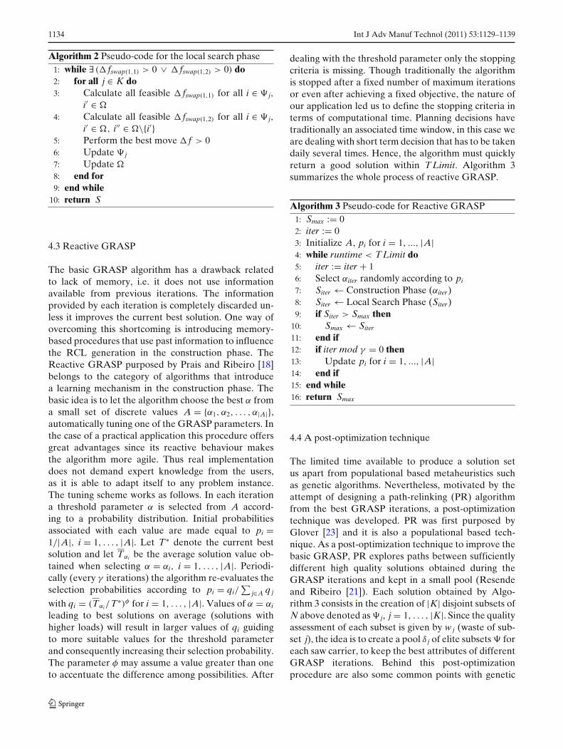
The neighbourhood search algorithm is designedaiming to be quickly performed assuring fast GRASPiterations, therefore only neighbourhoods resultingfrom the Swap(1, 1) and Swap(1, 2) are tested here.The purposed framework is presented in Algorithm 2.Let us additionally define � j as the set of bricks alreadyassigned to saw carrier j.

To improve the initially constructed solution, the lo-cal search algorithm proceeds similarly to the construc-tion phase. It analyses for one saw carrier at a time allfeasible solutions of the defined neighbourhoods (lines3–4). Then it performs the best move (line 5) updatingthe bricks sets (lines 6–7) before moving forward intothe next saw carrier. This design hybridizes the best-improving and the first-improving strategies. Once allpossible Swaps are investigated for one saw carrier ateach step but not for all carriers. The procedure endswhen � f ≤ 0 for every possible move.

1134 Int J Adv Manuf Technol (2011) 53:1129–1139

Algorithm 2 Pseudo-code for the local search phase1: while ∃ (� fswap(1,1) > 0 ∨ � fswap(1,2) > 0) do2: for all j ∈ K do3: Calculate all feasible � fswap(1,1) for all i ∈ � j,

i′ ∈ �

4: Calculate all feasible � fswap(1,2) for all i ∈ � j,

i′ ∈ �, i′′ ∈ �\{i′}5: Perform the best move � f > 06: Update � j

7: Update �

8: end for9: end while

10: return S

4.3 Reactive GRASP

The basic GRASP algorithm has a drawback relatedto lack of memory, i.e. it does not use informationavailable from previous iterations. The informationprovided by each iteration is completely discarded un-less it improves the current best solution. One way ofovercoming this shortcoming is introducing memory-based procedures that use past information to influencethe RCL generation in the construction phase. TheReactive GRASP purposed by Prais and Ribeiro [18]belongs to the category of algorithms that introducea learning mechanism in the construction phase. Thebasic idea is to let the algorithm choose the best α froma small set of discrete values A = {α1, α2, . . . , α|A|},automatically tuning one of the GRASP parameters. Inthe case of a practical application this procedure offersgreat advantages since its reactive behaviour makesthe algorithm more agile. Thus real implementationdoes not demand expert knowledge from the users,as it is able to adapt itself to any problem instance.The tuning scheme works as follows. In each iterationa threshold parameter α is selected from A accord-ing to a probability distribution. Initial probabilitiesassociated with each value are made equal to pi =1/|A|, i = 1, . . . , |A|. Let T∗ denote the current bestsolution and let Tαi be the average solution value ob-tained when selecting α = αi, i = 1, . . . , |A|. Periodi-cally (every γ iterations) the algorithm re-evaluates theselection probabilities according to pi = qi/

∑j∈A q j

with qi = (Tαi/T∗)φ for i = 1, . . . , |A|. Values of α = αi

leading to best solutions on average (solutions withhigher loads) will result in larger values of qi guidingto more suitable values for the threshold parameterand consequently increasing their selection probability.The parameter φ may assume a value greater than oneto accentuate the difference among possibilities. After

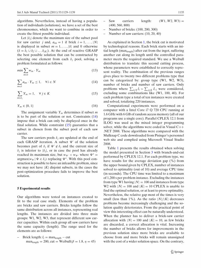
dealing with the threshold parameter only the stoppingcriteria is missing. Though traditionally the algorithmis stopped after a fixed number of maximum iterationsor even after achieving a fixed objective, the nature ofour application led us to define the stopping criteria interms of computational time. Planning decisions havetraditionally an associated time window, in this case weare dealing with short term decision that has to be takendaily several times. Hence, the algorithm must quicklyreturn a good solution within T Limit. Algorithm 3summarizes the whole process of reactive GRASP.

Algorithm 3 Pseudo-code for Reactive GRASP1: Smax := 02: iter := 03: Initialize A, pi for i = 1, ..., |A|4: while runtime < T Limit do5: iter := iter + 16: Select αiter randomly according to pi

7: Siter ← Construction Phase (αiter)8: Siter ← Local Search Phase (Siter)9: if Siter > Smax then

10: Smax ← Siter

11: end if12: if iter mod γ = 0 then13: Update pi for i = 1, ..., |A|14: end if15: end while16: return Smax

4.4 A post-optimization technique

The limited time available to produce a solution setus apart from populational based metaheuristics suchas genetic algorithms. Nevertheless, motivated by theattempt of designing a path-relinking (PR) algorithmfrom the best GRASP iterations, a post-optimizationtechnique was developed. PR was first purposed byGlover [23] and it is also a populational based tech-nique. As a post-optimization technique to improve thebasic GRASP, PR explores paths between sufficientlydifferent high quality solutions obtained during theGRASP iterations and kept in a small pool (Resendeand Ribeiro [21]). Each solution obtained by Algo-rithm 3 consists in the creation of |K| disjoint subsets ofN above denoted as � j, j = 1, . . . , |K|. Since the qualityassessment of each subset is given by w j (waste of sub-set j), the idea is to create a pool δ j of elite subsets � foreach saw carrier, to keep the best attributes of differentGRASP iterations. Behind this post-optimizationprocedure are also some common points with genetic

Int J Adv Manuf Technol (2011) 53:1129–1139 1135

algorithms. Nevertheless, instead of having a popula-tion of individuals (solutions), we have a set of the bestchromosomes, which we want to combine in order tocreate the fittest possible individual.

Let |δ j| denote the maximum size of the subset poolfor saw carrier j and, aim = 1 if brick i = 1, . . . , |N|is displayed in subset m = 1, . . . , |δ| and 0 otherwise(δ = δ1 ∪ δ2 ∪ . . . δ|K|). At the end of reactive GRASPthe best possible solution that can be constructed byselecting one element from each δ j pool, solving aproblem formulated as follows:

min∑

m∈δ

wm · Ym (13)

∑

m∈δ

aim · Ym ≤ 1, ∀ i ∈ N (14)

∑

m∈δ j

Ym = 1, ∀ j ∈ K (15)

Ym ∈ {0, 1} (16)

The assignment variable Ym determines if subset mis to be part of the solution or not. Constraints (14)impose that a brick can only be displayed once in thefinal solution. While constraint (15) guaranties that asubset in chosen from the subset pool of each sawcarrier.

The saw carriers pools δ j are updated at the end ofeach GRASP iteration. A subset � ′ of the solutionbecomes part of δ j if � ′ �∈ δ j and the current size ofδ j is inferior to |δ j|, or in case the pool has alreadyreached its maximum size, but w� ′ < w�∗ where �∗ =argmax(w� | � ∈ δ j) replacing �∗. With this pool con-struction is possible to have an infeasible problem, sincewe may not have |K| disjoint subsets, in the cases thepost-optimization procedure fails to improve the bestsolution.

5 Experimental results

Our algorithms were tested on instances created tofit to the real case study. Elements of the problemare bricks and saw carriers. Bricks lengths follow thesame distribution across all instances, representing reallengths. The instances are divided into three maingroups: W1, W2, W3, that represent different saw car-rier capacities. Within each group all saw carriers havethe same capacity (length). The range used for theelements are as follows:

– Brick length: li = maxlength − cutmaxlength = 200, cut = Weibull(β = 1.8, η = 45)

– Saw carriers length: (W1, W2, W3) =(400, 560, 800)

– Number of bricks: (100, 200, 300)– Number of saw carriers: (10, 20, 40)

As explained in Section 1, the brick cut is motivatedby technological reasons. Each brick starts with an ini-tial length (maxlength) after cut from the ingot, sufferinganother cut along its length until the controlled para-meter meets the required standard. We use a Weibulldistribution to translate this second cutting process,whose parameters were established to correctly repre-sent reality. The combination of the previous rangesgives place to twenty two different problems type thatcan be categorized by: group type (W1, W2, W3),number of bricks and number of saw carriers. Onlyproblems where

∑i∈N li >

∑j∈K L j were considered,

excluding some combinations like (W1, 100, 40). Foreach problem type a total of ten instances were createdand solved, totalizing 220 instances.

Computational experiments were performed on acomputer with a Intel Core i7 Q 720 CPU running at1.6 GHz with 6 GB of random access memory (all of ourprograms use a single core). Parallel CPLEX 12.1 fromILOG was used as the mixed integer programmingsolver, while the algorithms were coded in Visual C++.NET 2008. These algorithms were compared with theMulknap C code downloaded from Pisinger’s personnelweb site and complied using Microsoft Visual Studio2008.

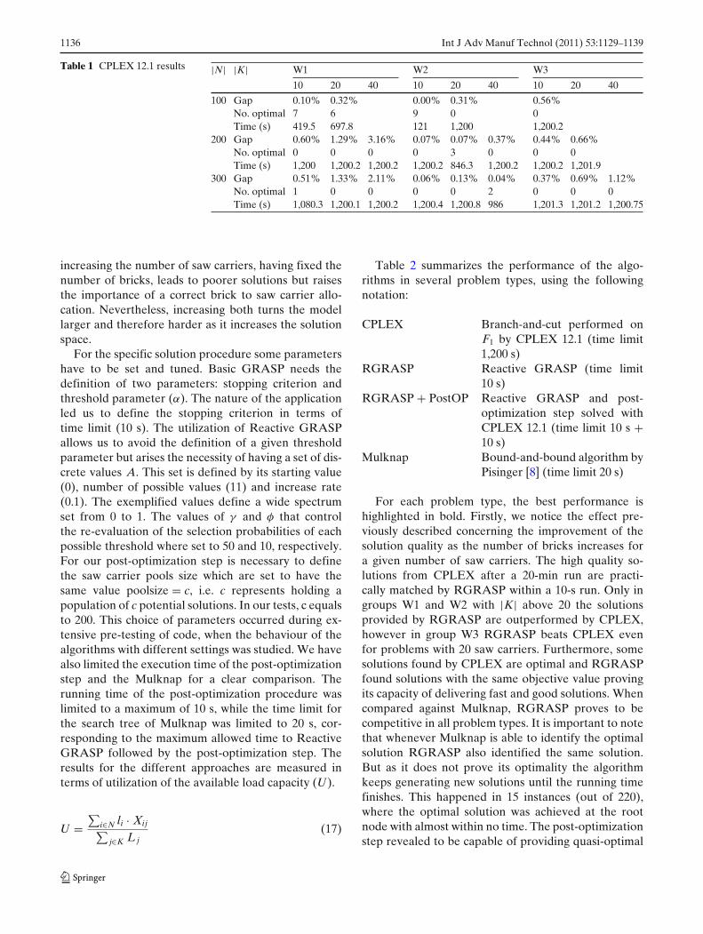
Table 1 presents the results obtained when solvingthe model presented in Section 3 with branch-and-cutperformed by CPLEX 12.1. For each problem type, wehave results for the average deviation gap (%) fromthe upper bound given by CPLEX, number of instancessolved to optimality (out of 10) and average CPU time(in seconds). The CPU time was limited to a maximumof 1,200 s per problem instance. Excluding the instancesfrom type W1 having |N| = 100 and instances from typeW2 with |N| = 100 and |K| = 10 CPLEX is unable tofind the optimal solution, or at least to prove optimality.Nevertheless, the relative gap most of the times is verysmall (less than 1%). As the ratio |N|/|K| decreasesproblems become increasingly challenging and the so-lution quality deteriorates. From the practical point ofview this interesting effect can be naturally understood.When the planner has to deliver a brick-saw carrierallocation with |N| = 100 and |K| = 10, as few bricksare discarded, a correct allocation is vital. Increasingthe number of bricks allows for improvements in theprevious solution since more bricks are available tochoose from and more bricks will remain unassignedwith the cost of a wider solution space. On the contrary,

1136 Int J Adv Manuf Technol (2011) 53:1129–1139

Table 1 CPLEX 12.1 results |N| |K| W1 W2 W3

10 20 40 10 20 40 10 20 40

100 Gap 0.10% 0.32% 0.00% 0.31% 0.56%No. optimal 7 6 9 0 0Time (s) 419.5 697.8 121 1,200 1,200.2

200 Gap 0.60% 1.29% 3.16% 0.07% 0.07% 0.37% 0.44% 0.66%No. optimal 0 0 0 0 3 0 0 0Time (s) 1,200 1,200.2 1,200.2 1,200.2 846.3 1,200.2 1,200.2 1,201.9

300 Gap 0.51% 1.33% 2.11% 0.06% 0.13% 0.04% 0.37% 0.69% 1.12%No. optimal 1 0 0 0 0 2 0 0 0Time (s) 1,080.3 1,200.1 1,200.2 1,200.4 1,200.8 986 1,201.3 1,201.2 1,200.75

increasing the number of saw carriers, having fixed thenumber of bricks, leads to poorer solutions but raisesthe importance of a correct brick to saw carrier allo-cation. Nevertheless, increasing both turns the modellarger and therefore harder as it increases the solutionspace.

For the specific solution procedure some parametershave to be set and tuned. Basic GRASP needs thedefinition of two parameters: stopping criterion andthreshold parameter (α). The nature of the applicationled us to define the stopping criterion in terms oftime limit (10 s). The utilization of Reactive GRASPallows us to avoid the definition of a given thresholdparameter but arises the necessity of having a set of dis-crete values A. This set is defined by its starting value(0), number of possible values (11) and increase rate(0.1). The exemplified values define a wide spectrumset from 0 to 1. The values of γ and φ that controlthe re-evaluation of the selection probabilities of eachpossible threshold where set to 50 and 10, respectively.For our post-optimization step is necessary to definethe saw carrier pools size which are set to have thesame value poolsize = c, i.e. c represents holding apopulation of c potential solutions. In our tests, c equalsto 200. This choice of parameters occurred during ex-tensive pre-testing of code, when the behaviour of thealgorithms with different settings was studied. We havealso limited the execution time of the post-optimizationstep and the Mulknap for a clear comparison. Therunning time of the post-optimization procedure waslimited to a maximum of 10 s, while the time limit forthe search tree of Mulknap was limited to 20 s, cor-responding to the maximum allowed time to ReactiveGRASP followed by the post-optimization step. Theresults for the different approaches are measured interms of utilization of the available load capacity (U).

U =∑

i∈N li · Xij∑j∈K L j

(17)

Table 2 summarizes the performance of the algo-rithms in several problem types, using the followingnotation:

CPLEX Branch-and-cut performed onF1 by CPLEX 12.1 (time limit1,200 s)

RGRASP Reactive GRASP (time limit10 s)

RGRASP + PostOP Reactive GRASP and post-optimization step solved withCPLEX 12.1 (time limit 10 s +10 s)

Mulknap Bound-and-bound algorithm byPisinger [8] (time limit 20 s)

For each problem type, the best performance ishighlighted in bold. Firstly, we notice the effect pre-viously described concerning the improvement of thesolution quality as the number of bricks increases fora given number of saw carriers. The high quality so-lutions from CPLEX after a 20-min run are practi-cally matched by RGRASP within a 10-s run. Only ingroups W1 and W2 with |K| above 20 the solutionsprovided by RGRASP are outperformed by CPLEX,however in group W3 RGRASP beats CPLEX evenfor problems with 20 saw carriers. Furthermore, somesolutions found by CPLEX are optimal and RGRASPfound solutions with the same objective value provingits capacity of delivering fast and good solutions. Whencompared against Mulknap, RGRASP proves to becompetitive in all problem types. It is important to notethat whenever Mulknap is able to identify the optimalsolution RGRASP also identified the same solution.But as it does not prove its optimality the algorithmkeeps generating new solutions until the running timefinishes. This happened in 15 instances (out of 220),where the optimal solution was achieved at the rootnode with almost within no time. The post-optimizationstep revealed to be capable of providing quasi-optimal

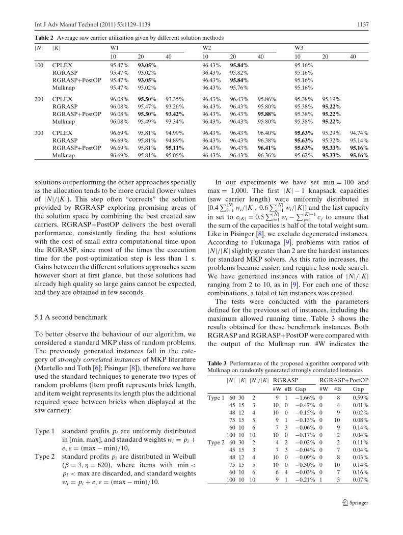
Int J Adv Manuf Technol (2011) 53:1129–1139 1137

Table 2 Average saw carrier utilization given by different solution methods

|N| |K| W1 W2 W3

10 20 40 10 20 40 10 20 40

100 CPLEX 95.47% 93.05% 96.43% 95.84% 95.16%RGRASP 95.47% 93.02% 96.43% 95.82% 95.16%RGRASP+PostOP 95.47% 93.05% 96.43% 95.84% 95.16%Mulknap 95.47% 93.02% 96.43% 95.76% 95.16%

200 CPLEX 96.08% 95.50% 93.35% 96.43% 96.43% 95.86% 95.38% 95.19%RGRASP 96.08% 95.47% 93.26% 96.43% 96.43% 95.80% 95.38% 95.22%RGRASP+PostOP 96.08% 95.50% 93.42% 96.43% 96.43% 95.88% 95.38% 95.22%Mulknap 96.08% 95.49% 93.34% 96.43% 96.43% 95.80% 95.38% 95.22%

300 CPLEX 96.69% 95.81% 94.99% 96.43% 96.43% 96.40% 95.63% 95.29% 94.74%RGRASP 96.69% 95.81% 94.89% 96.43% 96.43% 96.38% 95.63% 95.32% 95.14%RGRASP+PostOP 96.69% 95.81% 95.11% 96.43% 96.43% 96.41% 95.63% 95.33% 95.16%Mulknap 96.69% 95.81% 95.05% 96.43% 96.43% 96.36% 95.62% 95.33% 95.16%

solutions outperforming the other approaches speciallyas the allocation tends to be more crucial (lower valuesof |N|/|K|). This step often “corrects” the solutionprovided by RGRASP exploring promising areas ofthe solution space by combining the best created sawcarriers. RGRASP+PostOP delivers the best overallperformance, consistently finding the best solutionswith the cost of small extra computational time uponthe RGRASP, since most of the times the executiontime for the post-optimization step is less than 1 s.Gains between the different solutions approaches seemhowever short at first glance, but those solutions hadalready high quality so large gains cannot be expected,and they are obtained in few seconds.

5.1 A second benchmark

To better observe the behaviour of our algorithm, weconsidered a standard MKP class of random problems.The previously generated instances fall in the cate-gory of strongly correlated instances of MKP literature(Martello and Toth [6]; Pisinger [8]), therefore we haveused the standard techniques to generate two types ofrandom problems (item profit represents brick length,and item weight represents its length plus the additionalrequired space between bricks when displayed at thesaw carrier):

Type 1 standard profits pi are uniformly distributedin [min, max], and standard weights wi = pi +e, e = (max − min)/10,

Type 2 standard profits pi are distributed in Weibull(β = 3, η = 620), where items with min <

pi < max are discarded, and standard weightswi = pi + e, e = (max − min)/10.

In our experiments we have set min = 100 andmax = 1,000. The first |K| − 1 knapsack capacities(saw carrier length) were uniformly distributed in[0.4

∑|N|i=1 wi/|K|, 0.6

∑|N|i=1 wi/|K|] and the last capacity

in set to c|K| = 0.5∑|N|

i=1 wi − ∑|K|−1j=1 c j to ensure that

the sum of the capacities is half of the total weight sum.Like in Pisinger [8], we exclude degenerated instances.According to Fukunaga [9], problems with ratios of|N|/|K| slightly greater than 2 are the hardest instancesfor standard MKP solvers. As this ratio increases, theproblems became easier, and require less node search.We have generated instances with ratios of |N|/|K|ranging from 2 to 10, as in [9]. For each one of thesecombinations, a total of ten instances was created.

The tests were conducted with the parametersdefined for the previous set of instances, including themaximum allowed running time. Table 3 shows theresults obtained for these benchmark instances. BothRGRASP and RGRASP+PostOP were compared withthe output of the Mulknap run. #W indicates the

Table 3 Performance of the proposed algorithm compared withMulknap on randomly generated strongly correlated instances

|N| |K| |N|/|K| RGRASP RGRASP+PostOP

#W #B Gap #W #B Gap

Type 1 60 30 2 9 1 −1.66% 0 8 0.59%45 15 3 10 0 −0.47% 0 4 0.01%48 12 4 10 0 −0.15% 0 9 0.02%75 15 5 9 1 −0.13% 0 10 0.08%60 10 6 7 3 −0.06% 0 9 0.14%

100 10 10 10 0 −0.17% 0 2 0.04%Type 2 60 30 2 4 2 −0.02% 0 2 0.11%

45 15 3 7 3 −0.04% 0 7 0.04%48 12 4 10 0 −0.09% 0 8 0.03%75 15 5 10 0 −0.30% 0 10 0.14%60 10 6 6 4 −0.03% 0 7 0.16%

100 10 10 9 1 −0.21% 1 3 0.07%

1138 Int J Adv Manuf Technol (2011) 53:1129–1139

number of instances in which the output of the com-pared algorithm was worst than Mulknap and #B reg-isters the number of times the solution was better. TheGap column represents the average difference betweenthe output of the incumbent algorithm when comparedwith Mulknap: (z∗ − z)/z, where z is the solution pro-vided by Mulknap and z∗ the solution of the incumbentalgorithm.

Mulknap provided better solutions than RGRASPspecially in Type 1 instances, where the averagegap is bigger. The post-optimization step revelled itsefficiency again in these tests. Only in one out of120 instances the solution provided by Mulknap wasbetter than RGRASP+PostOP. The overhead of thepost-optimization step remains less than a secondon average. The number of solutions improved byRGRASP+PostOP does not appear to change amongthe two types, while the gap is more appealing inType 2. Looking at the effect of the different ratios(|N|/|K|) it is more evident in the borders of the range.For a ratio of 2 for Type 1 instances, RGRASP pre-sented its poorer performance and RGRASP+PostOPits better performance when compared with Mulknap.This attest the difficulty of these instances and alsothe effectiveness of the post-optimization step. As ex-pected from previous studies, Mulknap performs bet-ter when the ratio is increased to 10, in both typesof problems, leaving smaller room for improvementby RGRASP+PostOP. Once again optimal solutionsfound by Mulknap (12 out of 120) were matchedby RGRASP+PostOP, except in one case. Over-all RGRASP shown its competitiveness comparedwith Mulknap, specially if enhanced by the post-optimization step.

6 Conclusions

We give some insights into a scheduling problem thatarises during wafer slicing process in the photovoltaicindustry. Firstly, we model the problem, as a MultipleKnapsack Problem type. Secondly, as our case studydemands a real-world application with the ability of fastdelivering solutions, we have developed a quick localsearch algorithm. The algorithm is based on a greedyrandomized adaptive search procedure improved bya reactive mechanism. This mechanism allows the al-gorithm to self adapt to different problem instancesrepresenting a powerful feature to real-world applica-tions. Hence, little or none effort and knowledge fromusers is required during its utilization. Its effectivenessand performance are illustrated in a series of testsran on instances created from real ones and randomly

generated. In these tests, the algorithm was comparedwith a state of the art Multiple Knapsack Problem exactalgorithm (Pisinger [8]). The results show the capacityof the algorithm of delivering very good solutions inshort computational time enabling the creation of anon-line system to support production scheduling deci-sions. Such system can be a powerful tool to achievehigher throughput in the multi wire sawing process con-tributing for further wafer production cost reduction.Thirdly, to find better solutions we have developeda post-optimization procedure combining parts of thebest solutions found during the main algorithm.

Our algorithm can be easily adapted to solve otherMKP-type problems, pointing a possible area of futureresearch.

Acknowledgements The authors thank the four anonymousreferees for their useful comments and suggestions that helpedus improving the quality of the paper, and are also grateful toDavid Pisinger for making available the code of his algorithm.The first author is also grateful to the Portuguese Foundation forScience and Technology for awarding him a grant (SFRH/BD/62010/2009).

References

1. EPIA European Photovoltaic Industry Association andGreenpeace (2005) Solar generation v. Technical report

2. Swanson RM (2006) A vision for crystalline silicon pho-tovoltaics. Prog Photovolt: Research and Applications14(5):443–453

3. Jester TL (2002) Crystalline silicon manufacturing progress.Prog Photovolt: Research and Applications 10(2):99–106

4. Zulehner W (2000) Historical overview of silicon crystalpulling development. Mater Sci Eng B 73(1–3):7–15

5. del Cañizo C, del Coso G, Sinke WC (2009) Crystalline siliconsolar module technology: towards the 1 euro per watt-peakgoal. Prog Photovolt: Research and Applications 17(3):199–209

6. Martello S, Toth P (1990) Knapsack problems: algorithmsand computer implementations. Wiley, New York

7. Eilon S, Christofides N (1971) The loading problem. ManageSci 17(5):259–268

8. Pisinger D (1999) An exact algorithm for large multiple knap-sack problems. Eur J Oper Res 114(3):528–541

9. Fukunaga A (2009) A branch-and-bound algorithm for hardmultiple knapsack problems. Ann Oper Res. doi:10.1007/s10479-009-0660-y

10. Caprara A, Kellerer H, Pferschy U (2003) A 3/4-approximation algorithm for multiple subset sum. JHeuristics 9(2):99–111

11. Martello S, Toth P (1981) Heuristic algorithms for the multi-ple knapsack problem. Computing 27(2):93–112

12. Khuri S, Bäck T, Heitkötter J (1994) The zero/one multipleknapsack problem and genetic algorithms. In: Proceedingsof the 1994 ACM symposium on applied computing. ACM,Phoenix, Arizona, USA, pp 188–193

13. Raidl GR (1999) A weight-coded genetic algorithm for themultiple container packing problem. In: Proceedings of the1999 ACM symposium on applied computing. ACM, SanAntonio, Texas, USA, pp 291–296

Int J Adv Manuf Technol (2011) 53:1129–1139 1139

14. Fukunaga AS (2008) A new grouping genetic algorithm forthe multiple knapsack problem. In: IEEE congress on evolu-tionary computation, 2008. CEC 2008, IEEE world congresson computational intelligence, pp 2225–2232

15. Kellerer H, Pferschy U, Pisinger D (2004) Knapsack prob-lems. Springer, Berlin

16. Feo TA, Resende MGC (1995) Greedy randomized adaptivesearch procedures. J Glob Optim 6(2):109–133

17. Binato S, Hery WJ, Loewenstern DM, Resende MGC (2000)A grasp for job shop scheduling. In: Essays and surveys onmetaheuristics. Kluwer, Dordrecht, pp 59–79

18. Prais M, Ribeiro CC (2000) Reactive grasp: an application toa matrix decomposition problem in tdma traffic assignment.INFORMS J Comput 12(3):164–176

19. Adil GK, Ghosh JB (2005) Forming gt cells incrementallyusing grasp. Int J Adv Manuf Tech 26(11):1402–1408

20. Prabhaharanl G, Shahul Hamid Khan B, Rakesh L (2006)Implementation of grasp in flow shop scheduling. Int J AdvManuf Tech 30(11):1126–1131

21. Resende M, Ribeiro C (2003) Greedy randomized adaptivesearch procedures. Kluwer, Dordrecht. pp 219–249

22. Almada-Lobo B, Oliveira JF, Carravilla MA (2008) Produc-tion planning and scheduling in the glass container industry:a vns approach. Int J Prod Econ 114(1):363–375

23. Glover F (1996) Tabu search and adaptive memory pro-graming advances, applications and challenges. In: Inter-faces in computer science and operations research. Kluwer,Dordrecht, pp 1–75