Region-based adaptive slicing

Region-based adaptive slicing

K. Mani, P. Kulkarni, D. Dutta*

Department of Mechanical Engineering, The University of Michigan, Ann Arbor, MI 48109, USA

Received 19 October 1998; received in revised form 3 March 1999; accepted 12 March 1999

Abstract

In this paper, we describe a method for region-based adaptive slicing. Whereas in traditional adaptive slicing the user can impose a singlesurface finish (cusp height) requirement for the whole object, in region-based adaptive slicing, user has the flexibility to impose differentsurface finish requirements on different surfaces of the model. We describe the method and its implementation. Two example parts were builtusing the slicing technique and the results are included.q 1999 Elsevier Science Ltd. All rights reserved.

Keywords:Layered manufacturing; Slicing; CAD/CAM; Process planning

1. Introduction

1.1. Layered manufacturing

Layered manufacturing (LM) is a method for fabricationof physical parts, layer-by-layer, using computer control.An important characteristic of the method is that thegeometric complexity of the part is relatively unimportant.It is equally easy to manufacture a simple cube and acomplex object bounded by freeform surfaces. The accuracyof the manufactured object is directly related to slicing, akey process planning task.

1.2. Slicing for layered manufacturing

Slicing refers to intersecting a CAD model with a plane inorder to determine two dimensional contours on whichmaterial is to be deposited. The 2.5D entity formed bydepositing material inside the contour is referred to as alayer. The slicing can either be uniform, where the layerthickness is kept constant, or adaptive, where the layerthickness changes based on the surface geometry of theCAD model. Uniform slicing is commonly practiced inindustry. However, several inaccuracies can result whenemploying uniform slicing and are briefly described below.

1.2.1. Inaccuracies related to slicingThese inaccuracies are a direct consequence of manufac-

turing the part by stacking 2.5D layers.

1.2.1.1. Staircase inaccuraciesLayered manufacturedparts exhibit a staircase effect (see Fig. 1). Thisinaccuracy reflects the deviation of the surface of theCAD model from the vertically built LM part.

The error associated with the staircase effect can be quan-tified by considering the cusp height (d in Fig. 1). The cuspheight of a layerL is the maximum distance measured alonga surface normal, between the CAD surface and the layer.Uniform slicing typically results in an increase in the buildtime (many thin layers) or a poor surface finish (fewer thicklayers). A balance between the surface accuracy and buildtime is achieved by employing adaptive slicing.

1.2.1.2. Deposition inaccuraciesThis situation can beexplained using planar profiles as shown in Fig. 2.Between the CAD modelP and the manufactured objectQ, the following can occur:

(a) P # Q(b) Q # P(c) Q ÷ P andP ÷ Q

Situation (a) implies extra material has been deposited bythe LM process and a polishing operation can result in agood surface quality as well as the realization of the circularprofile. We refer to this condition as excess deposition.Situation (b) is referred to as deficient deposition and isuseful if the LM part is to act, for example, as a masterpattern for making cores. Situation (c) is clearly undesirableand the removal of cusps by polishing does not yield thedesired circular profile.

Computer-Aided Design 31 (1999) 317–333

COMPUTER-AIDEDDESIGN

0010-4485/99/$ - see front matterq 1999 Elsevier Science Ltd. All rights reserved.PII: S0010-4485(99)00033-0

www.elsevier.com/locate/cad

* Corresponding author. Tel.:1 1-734-936-3567; fax:1 1-734-647-3170.

E-mail address:[email protected] (D. Dutta)

1.2.2. Adaptive slicing

1.2.2.1. Concept and limitationsAdaptive slicing involvesslicing of the CAD model with varying layer thicknesses.For example, in [2], the user can specify a maximum allow-able cusp height for the object and also a deposition require-ment (excess or deficient). In order to achieve the userspecifications, surfaces of high curvature are sliced withthinner layer thicknesses and surfaces of low curvature aresliced with thicker layer thicknesses. Adaptive slicing yieldsbetter surface quality, as the staircase effect decreases andthe variations in the cusp height across the layers is mini-mized. The main advantage of adaptive slicing is that itgives the user explicit control over the surface quality.

However, most adaptive slicing routines use a singlecusp height for the whole model. This implies, allsurfaces have the same surface finish requirement.But, there are applications where certain part featuresare critical and only these features have specific surfacefinish requirements. This situation is analogous tomachining select surfaces on a cast part. In this paperwe describe a method for region-based adaptive slicing.It allows the user to specify distinct cusp height valuesfor different surfaces of the CAD model.

1.2.2.2. Prior work Prior work in slicing and adaptiveslicing for LM has been reported in [1–3,5,8–10]. For a

survey on various slicing methods and other processplanning tasks for LM, refer [13]. In all the aboveslicing strategies, the layer thickness varies only inthe vertical direction. Sabourin et al. [4] developed ahigh precision exterior, high speed interior slicingstrategy of STL models. The interior of the model issliced with thick layers and the exterior with adaptivelayer thicknesses. But, the surface finish requirementson all the surfaces of the model are restricted to bethe same. Tyberg [6] proposed a local adaptive slicingtechnique for a group of STL models. Each model issliced independently and the branches within a modelare also sliced independently. The surface finishrequirement on the group of models is restricted to bethe same. Krause et al. [7] describe a method for slicingin which the CAD model is decomposed into verticalsegments. Each segment is sliced independentlydepending on the surface finish requirement.

In this paper, we extend our earlier work [2] on adaptiveslicing of CAD models. We describe a slicing technique thatpermits the fastest layer manufacture of an object that hasdifferent surface finish requirements on different surfaces.The user can select surfaces of the model and for eachimpose a distinct cusp height requirement. Furthermore,for the whole model, a deposition condition (excess or defi-cient) can also be imposed. The method yields the slices aswell as an interference-free deposition sequence for theslices.

The balance of this paper is structured as follows. Section2 presents the decomposition of the CAD model into regionsand the layer thickness determination for each region. Thealgorithm for the region-based adaptive slicing scheme isdescribed in Section 3. We present implemented examplesin Section 4 and in Section 5 we remark on the applicabilityof the proposed slicing strategy for various LM processes.We conclude the paper in Section 6 and suggest some futureresearch tasks.

K. Mani et al. / Computer-Aided Design 31 (1999) 317–333318

Fig. 1. Staircase inaccuracies and cups height (d).

Fig. 2. Deposition inaccuracies.

2. Analysis of region-based adaptive slicing

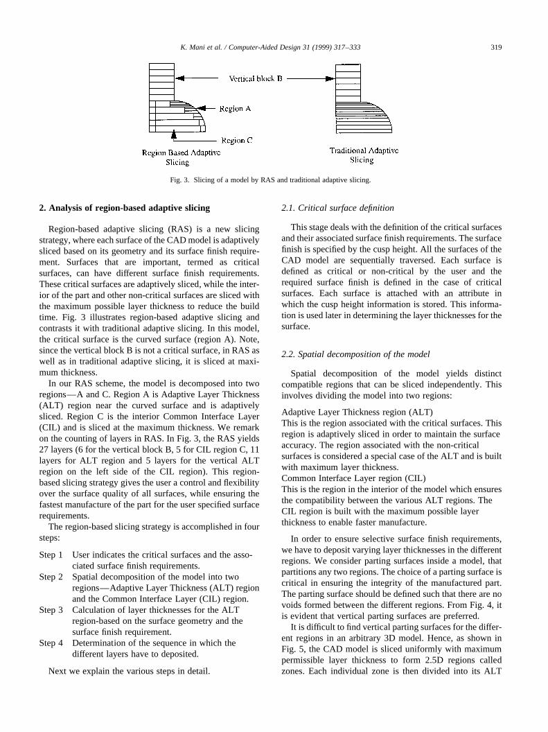
Region-based adaptive slicing (RAS) is a new slicingstrategy, where each surface of the CAD model is adaptivelysliced based on its geometry and its surface finish require-ment. Surfaces that are important, termed as criticalsurfaces, can have different surface finish requirements.These critical surfaces are adaptively sliced, while the inter-ior of the part and other non-critical surfaces are sliced withthe maximum possible layer thickness to reduce the buildtime. Fig. 3 illustrates region-based adaptive slicing andcontrasts it with traditional adaptive slicing. In this model,the critical surface is the curved surface (region A). Note,since the vertical block B is not a critical surface, in RAS aswell as in traditional adaptive slicing, it is sliced at maxi-mum thickness.

In our RAS scheme, the model is decomposed into tworegions—A and C. Region A is Adaptive Layer Thickness(ALT) region near the curved surface and is adaptivelysliced. Region C is the interior Common Interface Layer(CIL) and is sliced at the maximum thickness. We remarkon the counting of layers in RAS. In Fig. 3, the RAS yields27 layers (6 for the vertical block B, 5 for CIL region C, 11layers for ALT region and 5 layers for the vertical ALTregion on the left side of the CIL region). This region-based slicing strategy gives the user a control and flexibilityover the surface quality of all surfaces, while ensuring thefastest manufacture of the part for the user specified surfacerequirements.

The region-based slicing strategy is accomplished in foursteps:

Step 1 User indicates the critical surfaces and the asso-ciated surface finish requirements.

Step 2 Spatial decomposition of the model into tworegions—Adaptive Layer Thickness (ALT) regionand the Common Interface Layer (CIL) region.

Step 3 Calculation of layer thicknesses for the ALTregion-based on the surface geometry and thesurface finish requirement.

Step 4 Determination of the sequence in which thedifferent layers have to deposited.

Next we explain the various steps in detail.

2.1. Critical surface definition

This stage deals with the definition of the critical surfacesand their associated surface finish requirements. The surfacefinish is specified by the cusp height. All the surfaces of theCAD model are sequentially traversed. Each surface isdefined as critical or non-critical by the user and therequired surface finish is defined in the case of criticalsurfaces. Each surface is attached with an attribute inwhich the cusp height information is stored. This informa-tion is used later in determining the layer thicknesses for thesurface.

2.2. Spatial decomposition of the model

Spatial decomposition of the model yields distinctcompatible regions that can be sliced independently. Thisinvolves dividing the model into two regions:

Adaptive Layer Thickness region (ALT)This is the region associated with the critical surfaces. Thisregion is adaptively sliced in order to maintain the surfaceaccuracy. The region associated with the non-criticalsurfaces is considered a special case of the ALT and is builtwith maximum layer thickness.Common Interface Layer region (CIL)This is the region in the interior of the model which ensuresthe compatibility between the various ALT regions. TheCIL region is built with the maximum possible layerthickness to enable faster manufacture.

In order to ensure selective surface finish requirements,we have to deposit varying layer thicknesses in the differentregions. We consider parting surfaces inside a model, thatpartitions any two regions. The choice of a parting surface iscritical in ensuring the integrity of the manufactured part.The parting surface should be defined such that there are novoids formed between the different regions. From Fig. 4, itis evident that vertical parting surfaces are preferred.

It is difficult to find vertical parting surfaces for the differ-ent regions in an arbitrary 3D model. Hence, as shown inFig. 5, the CAD model is sliced uniformly with maximumpermissible layer thickness to form 2.5D regions calledzones. Each individual zone is then divided into its ALT

K. Mani et al. / Computer-Aided Design 31 (1999) 317–333 319

Fig. 3. Slicing of a model by RAS and traditional adaptive slicing.

and CIL regions. The CIL region ensures that the variousALT regions are boundary compatible by providing a verti-cal parting surface.

2.2.1. Determining CIL region in a zoneThe CIL region forms the interior of the zone and ensures

the boundary compatibility between the various ALTregions by providing vertical parting surfaces.

The CIL region is determined by analyzing the top andthe bottom slices of a zone. Fig. 6 shows examples of slicetopologies that need to be considered. The slices can becomposed of one or more contours. External contoursbound the model while internal contours are formed dueto voids in the model. The CIL is determined in two steps.

Step 1 Determine the ‘inner curves of intersection’ of theexternal contours and the ‘outer curves of inter-section’ of the internal contours.

Step 2 Determine the offsets to these curves of intersec-tion.

We elaborate on these two steps in the subsequent para-graphs.

2.2.1.1. Step 1: Determining the curves of intersectionThetop and the bottom slices of the zone are projected onto acommon horizontal plane. If the contours do not intersect,then one of the contours (bottom/top) will be completelycontained within the other (top/bottom). The contourcompletely contained is labeled the “inner curve”.

When the top and the bottom contours intersect, the“inner” and “outer” curves of intersection is found by aboolean intersection of the slices. This is done in order toensure that the offset to these curves of intersection, whenextruded from the bottom of the zone to the top, does notinfringe onto the surface of the model. Fig. 7(a) illustratesthe intersection of a contour from the top slice (dark) with acontour from the bottom slice (light). Also shown in Fig.

7(b,c) are the inner and outer curves of intersection of thecontour.

2.2.1.2. Step 2: Determining offsets to the curves ofintersection The inner curves of intersection are offsetby a positive distance, while the outer curves ofintersection are offset by a negative distance. A positiveoffset distance means that the offset curve is to the left,and negative offset distance means the offset curve is tothe right, of the curve of intersection when the curve ofintersection is traversed in the counter-clockwise (CCW)direction. The offset curves, determined for all the curvesof intersection, may or may not intersect each other. Offsetcurves that intersect are trimmed to ensure closed offsetcontours.

These offset contours are extruded down from the top tothe bottom of the zone to form a surface referred to asextruded-offset parting surface. This surface separates azone into exterior and interior regions. The interior regionof the zone is the CIL region and is deposited as a singlelayer, while the exterior region is composed of ALT regions.The extruded-offset parting surface is a vertical partingsurface and ensures the compatibility between the variousALT regions. The offset distance should be at least twice theroad width for depositing a contour. We chose the offsetdistance to be six times the road width to ensure properbonding between the various regions. The decompositionof the exterior region into the various ALT regions isdescribed in the next section.

2.2.2. Determining ALT regions in a zoneALT regions are sub-regions of the exterior region

mentioned in the previous paragraph. The sub-regionsnear the critical surfaces are deposited with adaptive thick-ness layers to maintain the surface quality. The sub-regionsnear the non-critical surfaces are deposited with maximumpermissible layer thickness to reduce the build time. The


Fig. 5. Spatial decomposition of a CAD model.

Fig. 4. Vertical parting surface between two different regions for compatibility.

decomposition of the exterior region into the various ALTsub-regions is done taking into account the surfaces thatbound the zone.

Recall that a slice of the zone can be composed of one ormore contours. Each contour is made up of distinct curvesegments. These segments are generated by the intersectionof the horizontal slicing plane with the surfaces that boundthe zone. We explain the determination of the ALT regionfor a critical surfaceS, that bounds a zone. SurfaceS isassociated with end pointsL and M (shown in Fig. 8(a)),on the extruded-offset surface, that are closest to the startand end points of the curve segment fromS in the bottomslice of the zone. Fig. 8(b) shows the contour of the ALTregion at heightZi. It comprises of four segments:

Segment 1Curve segment derived from surfaceSat heightZi.Segment 2This segment is part of the offset curve.Segment 3 and 4These are straight line segments PA and QB where, A and Bare points directly above L and M at heightZi.

The deposition requirements (excess or deficient) cannotbe satisfied by sweeping this contour (APQBA) from heightZi to Zi11 (whereZi11 is determined based on the layer thick-ness deposited). To satisfy the containment requirements,the inner or outer curves of intersections for the contours at

Zi andZi11 need to be determined (as explained in Section2.2.1). The contour of deposition is the outer curve of inter-section for excess deposition and the inner curve of inter-section for deficient deposition. The ALT region is thestack-up of all these contours of deposition evaluatedfrom the bottom of the zone to the top of the zone, basedon the layer thicknesses for the ALT region. The precedingdiscussion leads us to the following step-wise procedure forALT region determination.

Step 1 Determine points L and M on the offset contourthat are closest to the curve segment of surfaceSinthe bottom slice. The heightZi is set to the height ofthe bottom slice.

Step 2 Determine the layer thickness (Li) to be depositedfor the surface (described in the next section).

Step 3 Generate the contours atZi andZi11, whereZi11 is(Zi 1 Li). This contour comprises of the foursegments explained before in this section.

Step 4 Determine the inner/outer curve of intersection ofthe contours atZi andZi11, depending on the defi-cient/excess deposition requirement. IncrementZi

to Zi11.Step 5 Repeat steps 2 to 4 till the top of the zone is

reached.

Next we describe the calculation of layer thicknesses foran ALT region.

2.3. Layer thickness generation

The adaptive layer thicknesses for the ALT region in azone are determined based on the geometry, the surfacefinish requirements for the critical surfaces and the deposi-tion requirement as specified by the user. Layer thicknessgeneration starts from the bottom zone to the top zone.Within a zone layer thickness determination proceedsfrom bottom to top of the zone. TheZ height of the bottomand the top of the zone are referred to as bot_z and top_z,respectively.

The procedure we use for determining the layer thicknessis described in Ref. [2]. We summarize the method below.The slice obtained by slicing the model at bot_z comprisesthe various curve segments corresponding to the varioussurfaces that bound the zone. If the corresponding surfaceis non-critical, the layer thickness for the surface segment isset to ZT (zonal thickness). If the surface is critical, the cuspheight information is retrieved from the attribute stored withthe surface. Let curveC represent the curve segment of asurfaceS that bounds the model. In Fig. 9, Let P be a pointon the curveC. The vertical normal curvature of the surfaceS at the point P is determined. The normal section of thesurface at point P is locally approximated as a circle with theradius given by the reciprocal of the absolute value of thevertical curvature at point P. Using this circular approxima-tion at P, the optimal layer thickness at point P is foundbased on the deposition requirement (excess or deficient)


Fig. 6. Types of slices: (a) single contour slice; (b) multiple contour slice.

Fig. 7. Curves of intersection: (a) projected upper and lower slices; (b)inner curve of intersection; (c) outer curve of intersection.

and the cusp height requirement (d i) on that surface. Anoptimization procedure computes the layer thicknessd inFig. 9. See Ref. [2] for details.

TheZ height for the zone is incremented byd. The modelis sliced with a horizontal plane at this newZ height and thenew curve segment for surfaceS is determined. The nextlayer thickness is determined based on the new curvesegment and the cusp height. The above process is repeatedtill the Z height exceeds the top_z, i.e. the sum of the layerthicknesses for the ALT region is greater than or equal to thezonal thickness (ZT).

The deposition of layers in RAS is done zone by zone.Within a zone, the ALT regions are deposited first followedby CIL. This results in a constraint that the sum of thethicknesses of the adaptively sliced layers must equal theCIL thickness (ZT). Fig. 10 shows the cross section of azone with two ALT regions—A1 and A2. As it is evidentfrom the figure, for compatibility between zones, the sum ofthe layer thicknesses in each ALT regions A1 and A2 shouldbe equal to ZT. Hence, the final layer thickness is readjustedsuch that this constraint is satisfied. Similar layer thick-nesses are found for all the other surfaces in the zone.

2.4. Deposition sequence generation

After evaluating the layer thicknesses for each surface,the sequence for the deposition of layers has to be deter-mined based on the manufacturing constraint illustrated inFig. 11. The deposition of a layer takes place as shown inFig. 11(a).

Each ALT region yields a different set of layer thick-nesses. Therefore, at a particularz-height the deposition oflayers of different thicknesses might be required. Hence, it ispossible to encounter a situation shown in Fig. 11(b), wherethe nozzle interferes with the previously deposited material(P) while depositing region (R). To ensure an obstacle freepath for the nozzle, the smaller thickness region (R) shouldbe deposited before the thicker region (P). This manufactur-ing constraint requires a sequencing of the deposition of thelayers in the zone. The layers in the different ALT regionsare deposited in a sequence that ensures an obstacle free

path for the nozzle. The ALT regions are deposited firstand then the interior CIL region. The algorithm for thissequencing is described in Section 3.5.

The interplay between layer thicknesses in ALT regionsand sequence of deposition can sometimes result in subtleproblems. Consider Fig. 12(a) showing a zone in the frontview of a model composed of a spherical and a conicalsurface. This zone comprises of two ALT regions namely,the conical and spherical side ALT regions. The conical sideALT region is comprised of two layers say L1 (bottomlayer) and L2 (top layer). Similarly, the spherical sideALT region-based on different surface finish requirementmaybe comprised of four layers say S1, S2, S3 and S4from the bottom to the top of the zone. Fig. 12(b) showsthe top view of the zone with the ALT layers. From Fig.12(b), it is evident that there is no unique parting surfacebetween the ALT regions due to varying layer thicknesses.This leads to voids and overlapping of regions at the partingsurface between the ALT regions. If the sequence of deposi-tion is, for example, S1, S2, L1, S3, S4, L2, when S2 isdeposited on S1, the regions under the dark shaded portionsare voids (shown in Fig. 12(c)). Similarly, there is an over-lap between the layers L1 and S2. But these imperfectionsoccur in very small regions and does not affect the overallbuilding procedure or the surface quality of the parts (as willbe seen in the examples manufactured).


Fig. 9. Normal vertical section.

Fig. 8. (a) Top view of bottom slice; (b) top view of a contour in ALT region.

3. Algorithm

The input to RAS is an ACIS.sat model, cusp heightsd ison the critical surfaces, minimum and maximum allowablefabrication thicknesses,Lmin andLmax. The slices are outputin the Stratasys SLC format.

The flow chart for the proposed algorithm is shown in Fig.13. The initial Pre-Processingstep is performed on themodel to prepare it for the RAS procedure. Next, the bottomzone for the model is generated with maximum layer thick-ness.Contour analysisis required to ensure that the localchanges in geometry and topology are captured inside azone. The next step,offset evaluation, determines theboundary of the CIL region which forms the vertical partingsurface. The individual layer thicknesses are then deter-mined in the layer thickness calculationstep. The finalstep in the procedure is thecontour evaluation, where theboundaries of the ALT region and the order in which theALT regions are deposited, is determined. Each of the fivesteps is elaborated in the following sub-sections.

3.1. Pre-processing

Pre-processing of the model is done in three steps asshown in Fig. 14.

The first two steps are pre-processing steps on thesurfaces that bound the model. Set_Cusp_Height initializesthe cusp height requirement for each surface of the modeland Set_Surface_Tags places a unique tag on each surface.All the surfaces that bound the model are sequentiallytraversed and highlighted. The user is given the option ofdefining the particular surface highlighted as either criticalor non-critical. For critical surfaces, the required surfaceaccuracy is specified by the cusp height. These cusp heightsare stored asattributes on the surfaces using the ACIS

geometric kernel. This data can then be retrieved whilecalculating the layer thickness for each surface.

The final step, Block_Division, is the procedure to ensurethat sharp features, like the vertices, are not missed. This isthe same procedure as described in Ref. [2]. At the verticesof an object, the procedure used for layer thickness calcula-tion (Section 2.3) may result in erroneous results as shownin Fig. 15. At point P, the layer thickness determined by thecircular approximation is, say,d. Depositing a layer ofthicknessd will miss the vertex. Thus, to ensure the verticesare not missed, the model is first sliced at each vertex. Thevertices are then stored by theZ coordinates and the portionbetween two successive vertices is referred to as a “block”.Each block is then divided into zones in order to performRAS.

The output from the pre-processing step is:

• SetS—All the surfaces that bound the model.• Set C—All the critical surfaces of the model. These

surfaces may have different surface finish requirements.Note: C # S

• Set B—Blocks obtained by intersecting planes passingthrough the vertices.

3.2. Contour analysis

The aim of the contour analysis is to ensure that the“surface associativity” condition is satisfied within thezone. Surface associativity refers to the condition wherethe number of contours and their progenitor surfaces inthe upper and the lower slices of the zone are the same.

Recall, that the zones are created from the bottom to thetop of a block by slicing uniformly with maximum permis-sible layer thickness. Local geometry changes within thezone can create a mismatch between the upper and thelower contours of the zone. The aim of contour analysis is


Fig. 11. (a) Layer deposition in FDM; (b) obstruction.

Fig. 10. Cross section of a zone.


Fig. 13. Flow chart.

Fig. 12. Voids and overlapping regions at the common boundary: (a) zone; (b) top view of the zone; (c) top view of ALT (spherical slide).

to detect such mismatches and to create a transition zonewhose upper and lower slices do not have any mismatch,i.e., satisfy surface associativity. Let NB (NT) denote thecontours on the lower (upper) slice and SB (ST) the corre-sponding progenitor surfaces. As illustrated in Fig. 16, eachzone when created is checked for the surface associativitycondition. When SB± ST, a transition zone (from thebottom to some intermediate thickness) within the originalzone is determined. This transition zone ensures that theprogenitor surfaces, of the upper and the bottom slices ofthe transition zone, are the same. Similarly, if NB± NT forthe newly determined transition zone or the original zone (ifSB � ST), another transition zone is created. This finaltransition zone satisfies the surface associativity conditionand is used for further processing. The next zone is obtainedby slicing with maximum layer thickness from the upperslice of the final transition zone, which is then tested forsurface associativity. In the subsequent paragraphs, weelaborate on how to deal with situations when the surfaceassociativity condition is not satisfied.

1. When the progenitor surfaces are the same in the upperand the lower slices of the zone (SB� ST): The sub casesare:

(a) When the number of contours are the same(NB �NT): In such situations, we assume that there is nopossibility of any local changes within the zone. Thisassumption is valid as the maximum layer thickness isof the order of a thousandth of an inch (0.015 in forFDM) and the variations within the zone is nearlyimpossible.(b) When the number of contours are different(NB ±

NT): This is typically the case, when the surfacebranches are as shown in the Fig. 17.Layer thickness calculation is done from the bottom tothe top of the zone. Determining the layer thickness inthis fashion can result in overlooking the point P. Toeliminate these inaccuracies, point P is determined andthe model is sliced at this height to form a transitionzone from the bottom of the zone to the slice at P. Thistransition zone satisfies the surface associativity andcan be decomposed into the ALT and the CIL regions.Note that the zonal thickness of the transition zone isless thanLmax.

2. When the progenitor surfaces are different in the upperand the lower slices of the zone (SB± ST):Fig. 18 depicts a situation where the progenitor surfacesof the upper and the lower slices of the zone are different.This zone has two progenitor surfaces at the bottom slice,namely, the spherical and the conical surfaces. At the toponly the conical surface is present. The point P, where theconical and spherical surface meet, is not a point of hori-zontal tangency. Since the layer thickness calculation isdone from the bottom of the zone to the top, point P canbe missed. So we may end up with a situation shown inFig. 18(b), where the last layer deposited on the sphericalside (Lsphere) overshoots point P into the conical region.But for the conical surface at the bottom slice, the layerthickness (Lcone1) is calculated independently from thebottom of the zone. This results in unequalZ heights(Lcone1 and Lcone2) for the same conical ALT region. Toovercome this situation, a transition zone is formed fromthe bottom slice to the slice at P (Fig. 18(c)). This transi-tion zone has the same set of surfaces at the upper and thelower slices of the zone. After this a check is made on thenumber of contours to ensure that there are no localchanges within the newly formed zone.

The contour analysis algorithm described below deter-mines the transition zone for zones with local changes.

Algorithm Contour_AnalysisInput : Top_Slice, Bot_SliceOutput : Zone satisfying “surface associativity”


Fig. 15. Error introduced by the presence of a vertex.

Fig. 14. Pre-processing steps.

begin(ST,SB)( Set of the progenitor surfaces in upper and

lower slices of the zone(NT,NB)( Number of contours in the upper and lower

slices of the zoneif SB± STthen

evaluate_transition_ZT(condition: SB� ST)evaluate_new_upper_slice(ZT)

if NB ± NT thenevaluate_transition_ZT(condition: NB� NT)evaluate_new_lower_slice(ZT)

endreturn ZT

end

The function evaluate_transition_ZT determines the ZTfor the new zone used in the analysis. This evaluates the newZT in an iterative procedure until no local change happensin a zone. As seen from the algorithm, contour analysis isdone in two steps. The first step is a check on the equality ofthe set of progenitor surfaces in the upper and lower slices.Next step is a check on the equality of the number ofcontours in the upper and lower slices of the zone. Afterpassing these two checks, the zone would satisfy the surfaceassociativity.

3.3. Offset evaluation

Offset evaluation is required for the generation of the

parting surface between the CIL and the ALT regions.Recall that the decomposition of the exterior region intovarious ALT regions is dependent on these offset contours.A slice can have one or more external contours. Each exter-nal contour corresponds to a branch of the object. In thisstep, we evaluate the ALT and the CIL regions within eachbranch. Each branch has an external contour and its internaland offset contours. These contours are grouped together toform a ‘cluster’. We also use the term cluster to representthe set of surfaces comprising the group (Fig. 19).

There are cases when it is not possible to decompose thebranch into the ALT and the CIL regions. Such cases, asdescribed below, are identified and the cluster (representingthe branch) is classified as RAS_feasible or RAS_infeasible.

1. CIL region does not exist in the cluster: CIL region in thecluster may not exist because the offset distance may betoo large. Fig. 20(a) shows the case when the offsets toboth the external and internal contours lie outside theboundaries of the model. Fig. 20(b) shows the casewhen no offset curve exists because of a large offsetdistance. Such cases are again manufactured with theminimum of the layer thicknesses determined for eachsurface segment in the contour. In these situations we seethat there is no CIL region defined.

2. CIL regions resulting due to the intersection of the offsetcontours: This results in the ambiguity in the definition ofthe ALT regions. Consider a solid sphere with a cylind-rical void eccentric from the center. Both the sphericaland the cylindrical surfaces can be critical with differentsurface finish requirements. Fig. 20(c) shows the topview of the bottom slice of a zone and the offset contour.It is not possible to define the ALT regions for the twosurfaces since the two offset contours intersect eachother. In such cases, the exterior region is manufacturedas a single region just as in conventional adaptive slicing.The layer thickness is the minimum of the layer thick-nesses determined for the sphere and the cylinder indivi-dually, hence maintaining the cusp height requirement onboth the surfaces.

3. Case of infeasibility, when the offset contours do notintersect: These are the situations when the offsets tothe contours in the cluster do not intersect. But, due tosmall feature sizes, it is not possible to define ALTregions for some surfaces in the cluster. Fig. 20(d)shows a bottom slice comprising of one external contourand its offset. The curve segment A is from a criticalsurface. It is not possible to define an ALT region forthis surface. Such cases are again manufactured as adap-tive exterior region and a single interior region (CIL) ofmaximum layer thickness.

The algorithm below describes the offset curves and clas-sifies the clusters. The curves of intersection are determinedas explained in Section 2.2.1. Offsets to these curves ofintersection form the contours of deposition for the CILregion.


Fig. 17. Surface branching.

Fig. 16. Cases that arise by comparing the upper and the lower slices of thezone.

Algorithm_Offset_EvaluationInput : Top_Slice, Bot_SliceOutput : Offset contoursbegin

generate_curves_of_intersection(Top_Slice,Bot_Slice)

generate_offset_contours(curves of intersection)if (Offset_Contours� NULL) then

Adaptive_Slicing(zone)else

form_groups_and_clusters(Bot_Slice)check_RAS_feasible_clusters(C-Set of clusters)

end {if}end

3.4. Layer thickness calculation

This procedure retrieves the cusp-height informationfrom the surfaces and calculates the layer thicknesses forthe ALT regions. Before evaluating the layer thicknesses forindividual ALT regions, we determine if any surface yields

more than one curve segment in the bottom slice. Fig. 21shows one such model, which when sliced yields two curvesegments from the same surface S1. Though the curvesegments are from the same surface (same cusp height),circular approximation during layer thickness calculation(Section 2.3) may yield different layer thicknesses foreach curve segment. Hence, we need to define sub-regionswithin an ALT region. Every curve segment from the samesurface is associated with sub-regions near them. Tags areplaced on curve segments from the same surface in thebottom slice to distinguish one from the other. The layerthicknesses for each sub-region is then evaluated indepen-dently.

If a cluster is RAS-infeasible, then the layer thickness isdetermined as in traditional adaptive slicing. The minimumof the layer thicknesses evaluated for the tagged surfaces inthe cluster is set as the layer thickness for all the surfaces inthe cluster. For RAS-feasible clusters, the layer thicknessesare evaluated individually for each surface segment tag inthe cluster.

Evaluating layer thicknesses from the bottom to the top of


Fig. 19. A bottom slice of the zone with the clusters.

Fig. 18. Zone with surface non-associativity.

a zone can lead to situations where the final layer thicknessfor an ALT region may be less thanLmin. In such cases, aredistribution of layer thicknessesis done. We explain thiswith an example. Let the ZT be 0.015 in. The maximum(Lmax) and minimum (Lmin) allowable fabrication layer thick-nesses are 0.015 and 0.003 in, respectively. Let an ALTregion be composed of three layers. The layer thicknessesfor the first two layers (L1 andL2) being 0.006 and 0.007.The final layer thickness determined from the circularapproximation is, say, 0.007. Due to the constraint on thelayer thicknesses, the layer thickness (L3) for the third layerhas to be 0.002. But, this is lesser thanLmin and is notmanufacturable. In such situations, the layer thicknessesare redistributed such that the final layer thickness isLmin.In this case,L2 is reassigned as 0.006 andL3 is 0.003. Thiswill ensure that the cusp height requirement on all thesurfaces is satisfied.

Algorithm_evaluate_layer_thicknessesInput : Bot_Slice, Set C, E/D - excess/deficient depositionrequirement

Output : Layer thicknesses for all the ALT regions.begin

set_surface_segments_tags(Bot_Slice)TCi ( Represents the set of tagged surfaces in cluster

Ci

while (C ± 0) doIf (Ci ! RAS_feasible� TRUE) then

while (TCi ± 0) doevaluate_layer_thickness(TCi, E/D)

elseevaluate_layer_thickness(Ci, E/D)

end {if}end {while}

end

3.5. Contour evaluation

Contour evaluation involves generating the boundariesof the various contours of deposition and determiningthe sequence of their deposition to ensure that the


Fig. 21. (a) Model; (b) slice atZ.

Fig. 20. Top view of the bottom slice; (a) offsets to the contours intersect; (b),(c) offset distance is large; (d) special cases of infeasibility.

manufacturing constraint is satisfied. Recall, that a cluster isformed by mapping the external and internal contours withthe offset contours in the bottom slice. Each contour (exter-nal/internal) is associated with a unique offset contour in aRAS-feasible cluster. Contour evaluation for the ALTregions proceeds by mapping the surface segments in thebottom slice with points on the offset contour as explainedin Section 2.2.2. Although this mapping is from a curve tocurve, it is actually a mapping of the surface segment tagswith a corresponding set of points on the offset contour. Thesame set of offset points are used for the contours in an ALTregion. The various contours are deposited in such a waythat theZ level of the nozzle is always above the alreadydeposited layers. This ensures that the manufacturingconstraint is not violated.

Algorithm_Contour_EvaluationInput : Set S, Set C, Set TCi Bot_Slice, E/D-excess/defi-cient depositionOutput : Contours of deposition in sequencebegin

check_all_layers_max() {returns all_max_layersUTRUE if all layers are maximum}

if (all_max_layers� TRUE) thengenerate_complete_contour(Bot_Slice, E/D)

elsez � bottom of the zoneTCij ( representsjth tag in the setTCi

while C ± 0 dowhile TCi ± 0 do

If (RAS_feasible)thenevaluate_offset_pts_for_ALT_contour(Bot_-

Slice,TCij)dij � current_layer_thickness(TCij)setzij � z 1 dij

end {while}end {while}Do

MTC( Tagged surface with minimumZ heightMC( Cluster to which MTC belongsIf (MC ! RAS_feasible� TRUE) then

generate_alt_slice(MTC, E/D)update_current_layer_thickness(MTC)update_cur_z(MTC)

elsegenerate_cluster_as_a_single_slice(MC, E/D)update_layer_thickness(MC)update_z

until (all ALT layers deposited)generate_CIL_layer(zone)

end

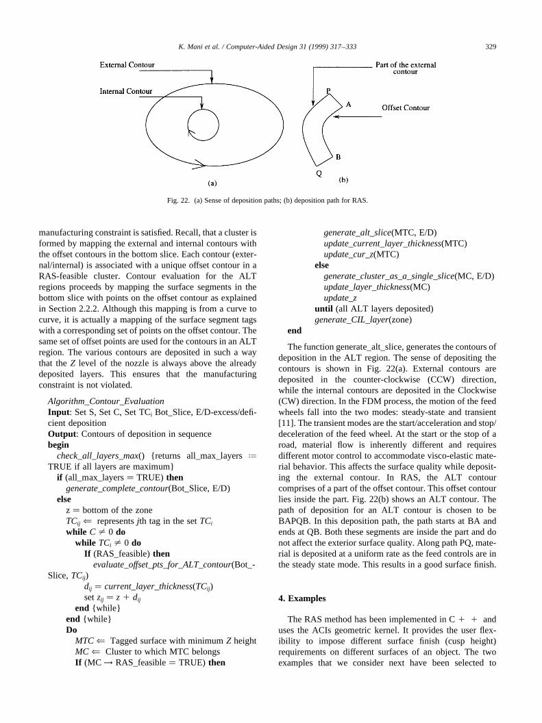
The function generate_alt_slice, generates the contours ofdeposition in the ALT region. The sense of depositing thecontours is shown in Fig. 22(a). External contours aredeposited in the counter-clockwise (CCW) direction,while the internal contours are deposited in the Clockwise(CW) direction. In the FDM process, the motion of the feedwheels fall into the two modes: steady-state and transient[11]. The transient modes are the start/acceleration and stop/deceleration of the feed wheel. At the start or the stop of aroad, material flow is inherently different and requiresdifferent motor control to accommodate visco-elastic mate-rial behavior. This affects the surface quality while deposit-ing the external contour. In RAS, the ALT contourcomprises of a part of the offset contour. This offset contourlies inside the part. Fig. 22(b) shows an ALT contour. Thepath of deposition for an ALT contour is chosen to beBAPQB. In this deposition path, the path starts at BA andends at QB. Both these segments are inside the part and donot affect the exterior surface quality. Along path PQ, mate-rial is deposited at a uniform rate as the feed controls are inthe steady state mode. This results in a good surface finish.

4. Examples

The RAS method has been implemented in C1 1 anduses the ACIs geometric kernel. It provides the user flex-ibility to impose different surface finish (cusp height)requirements on different surfaces of an object. The twoexamples that we consider next have been selected to


Fig. 22. (a) Sense of deposition paths; (b) deposition path for RAS.

highlight the following points. First, RAS should yieldfaster build times compared to traditional adaptive slicing.This is because the interior of an RAS object is built fasterand the fact that even within a zone, only surfaces with cuspheight requirements are sliced accordingly, the othersurfaces are sliced at maximum layer thickness. The secondpoint to be made is that this discriminatory slicing within azone can result in small raster lengths and increased ancil-lary functions (indexing, idle motions, etc.). Consequently,there is likely to be a threshold size (of an object) belowwhich RAS might not yield faster manufacture.

4.1. Example 1

Shown in Fig. 23(a) is the solid model of a part. Alsoshown in Fig. 23(b) and (c) are the front and the top viewswith dimensions in inches. The model was sliced by RASand by the ASM (Adaptive Slicing Method referred to inRef. [2]). In both cases, the minimum layer thickness (Lmin)was set to 0.002 in while the maximum layer thickness(Lmax) was 0.015 in. Both models were fabricated by theStratasys FDM machine. Table 1 shows the data and theresults obtained for both slicing strategies. In RAS, weimpose a cusp height of 0.003 on the cylindrical surfaces,while no surface finish requirement is given on the rib. Thecylindrical surfaces are adaptively sliced to maintain thecusp height requirement and other surfaces are sliced withmaximum layer thickness. Cusp height for the whole objectwhen using ASM, was chosen to be 0.003, to meet thesurface finish requirement on the cylindrical surfaces.

4.1.1. Results and discussionThe ALT regions ensures that the surface finish require-

ments are satisfied on the individual cylindrical surfaces.The layer thicknesses for the cylindrical side ALT regionsranged from 0.003 to 0.015 in, while the vertical surfacesand the rib surface were deposited with maximum layerthickness. The time to manufacture the model reduced by23% when RAS was used instead of ASM. The RAS yields903 layers, counted as explained in Section 2. The largernumber of layers in RAS does not result in longer time tomanufacture. Since the CIL region and the non criticalsurfaces are manufactured with maximum layer thickness,it decreases the overall time to manufacture.

4.2. Example 2

Now we consider an object from Ref. [4] and it is illus-trated in Fig. 24(a). Fig. 24(b) and (c) shows the front andthe top views of the object. We keep the same overalldimensions (0.4 in thick and 1.18 in wide) as in Ref. [4]and assume the curved surface is part of a torus. Accord-ingly we use 0.86 in as the radial width of the object asshown in the top view (Fig. 24(c)). As in Ref. [4], we specifya single cusp height of 0.005 in for the model and use0.015 in and 0.005 in as the maximum and minimum layerthicknesses, respectively.

This object was manufactured on the Stratasys FDMusing RAS and ASM in Ref. [2]. Results are shown inTable 2. Also, included are the results from Ref. [4]although meaningful comparisons cannot be made sincethe test part similarities have not been verified.


Fig. 23. (a) Solid model of Example 1; (b) front view of Example 1; (c) top view of Example 1.

Table 1

Cusp heights used (in) Number of layers Build time (minutes)

Adaptive slicing (ASM) 0.003 on all surfaces 213 508Region-based adaptive slicing (RAS) 0.003 on both the cylindrical surfaces 903 391

4.2.1. Results and discussionRAS yielded layers of maximum thickness for the vertical

surfaces, while the curved surfaces were adaptively sliced.However, for this example RAS required more time thanASM, contrary to our expectations. This can be attributed tothe following:

• Since the number of layers in RAS is greater than inASM, excess wait times were introduced betweenlayers.1 This excess time is usually offset by the deposi-tion of the CIL region and the non-critical ALT regionswith maximum layer thickness. But, in this particularexample, the (small) size of the model was a factor.Fig. 25(a) shows the top view of the bottom slice withthe boundaries of the ALT regions. The ALT regionscorresponding to the vertical surfaces were very small(Fig. 25(a)). Hence depositing them as separate layersincreases the time. One way to overcome this situationis to deposit the CIL and the non-critical ALT regions asa single compound layer of maximum thickness (Fig.25(b)).

• Up to aZ height of 0.255 in, all layers were of maximumthickness and were deposited as a single layer in RAS as

well as in ASM. The curved surface yielded layer thick-nesses in the range of 0.008–0.010 in after aZ height of0.255 in. Most of the layers were of 0.010 in thicknesses.In ASM, these layers are deposited as single layers of0.01 in thickness. But, in RAS we deposit layers of thick-nesses 0.010 in, 0.005 in due to the constraint on thelayer thicknesses in a zone. This deposition of smallerthickness layers, also resulted in increasing the buildtime.

Both the factors above point to the fact that the economiesof scale come into play. To test the hypothesis, the samemodel (Example 2) was scaled up by a factor of 2 andmanufactured after slicing by ASM and RAS. The resultsare shown in Table 3. The expected savings in time tomanufacture using RAS are realized for this larger model.

This indicates that there is a threshold size for a given setof parameters on a model, after which RAS will yieldsavings in time with respect to ASM. We investigate thisfurther.

The theoretical time to manufacture using ASM can beobtained using

TASM � 1R× V

� � XNASM

i�1

Ai 1 NASM·WT �1�

whereNASM is the number of layers in ASM,R the road


Fig. 24. (a) Solid model of Example 2; (b) front view of the model; (c) top view of the model.

1 In FDM, the machine needs to index its height after finishing eachlayer. This adds to the overall build time.

Table 2


Adaptive slicing (ASM) 0.005 33 44Region-based adaptive slicing (RAS) 0.005 81 46High precision exterior, high speed interior 0.005 38 49

width, V the speed of the nozzle,WT the indexing time andAi the area of deposition for theith layer.

Similarly, for RAS, the theoretical time to manufacture

TRAS � 1R× V

� �XNz

z�1

XNsz

j�1

XNljz

i�1

�AALT �ijz� 1 ACIL�z��0@ 1A

1 �NRAS·WT� �2�whereR, V and WT are as defined earlier. OnlyAi is nowreplaced by the sum of the areas of the ALT and CIL regionsfor each zone �PNsz

j�1

PNljz

i�1 �AALT �ijz� 1 ACIL�z�� and issummed over allNz zones.

The theoretical times for RAS and ASM slicing strategieswere calculated using Eqs. (1) and (2). Table 4 shows thatthe theoretical times do provide a lower bound for the buildtime. An indexing wait time (WT) of 4.48 s, determinedexperimentally, was used. A nozzle speed of 0.7 in/s and aroad width of 0.02 in (from actual manufacture) were usedin Eqs. (1) and (2).

Table 5 compares the theoretical build time for differentscales of the object in Example 2, using RAS and ASM. Ascan be seen, the cross over point (to realize benefits of RAS)is, for this particular example, a scale factor of 1.25.Economies of scale do exist and the extra work done inRAS (indexing, nozzle turns, etc.) is not without cost. The

theoretical build times can be used, prior to manufacture, todetermine if indeed RAS will yield a faster build. In general,for large complex objects RAS is likely to result in fastermanufacture.

5. Applicability to rapid prototyping processes

RAS has been successfully tested with Fused DepositionModeling (FDM)1 process. This slicing strategy is alsoapplicable to methods like Stereolithography (SLA) andSelective Laser Sintering (SLS). However, the physics ofthe SLA and SLS processes have to be taken into accountand might lead to modification to the algorithm presented.

In SLA, work area is spread with a thin layer of photo-polymer in which each cross sectional layer of the model isformed using a laser beam to solidify the layer of resin. Aseach layer is solidified, an elevator platform lowers theworkpiece to allow another layer of resin to be applied. Awiper smooths the layer to the proper thickness and the nextlayer is drawn, adhering it to the previous layer. The wiperintroduces the constraint on manufacturing explained inSection 2.2.1. The parting surface between the variousregions should be vertical, which is ensured in RAS.

In SLS, a high-power laser traverses a thin layer ofpowder in order to sinter the powder onto a previous


Fig. 25. Top view of the bottom slice with the ALT region boundaries marked: (a) small ALT regions (vertical surfaces); (b) compound layer (CIL and the non-critical ALT layer).

Table 3


Adaptive slicing (ASM) 0.005 66 317Region-based adaptive slicing (RAS) 0.005 175 295

layer. A roller does the job of the wiper in SLA. The rollerevenly distributes the powder on the bed. Hence, theconstraints discussed for FDM also applies to SLS. Carefulmodulation of the laser beam can ensure the adjacentregions are not affected while the laser beam cures thelayer. In all the three processes, the layer thickness can bevaried during fabrication.

6. Conclusions and suggestions for future work

A slicing strategy was described, where each surface ofthe CAD model was adaptively sliced based on its surfacefinish requirement and geometry. This new strategy givesthe user flexibility in defining the surface accuracy specifi-cation for the CAD model and also ensures the fastest manu-facture of the object. Two sample models were sliced usingthe algorithm and fabricated using the Stratasys 3D mode-ler. The time to manufacture the first example was found tobe lesser than that by traditional adaptive slicing routines,while the second one showed that the economies of scaleplay a role in the build time assessment. In general, thisslicing procedure is likely to yield better results for themanufacture of large complex parts which have surfacefinish requirements only on few critical surfaces. Thiswork can be further expanded to include heterogeneousmodels. A method for adaptive slicing of heterogeneousobjects (objects with varying material composition/micro-structure) taking into account both geometry and materialbased issues was presented in Ref. [12]. Similar to this work,the idea of region-based slicing can also be applied toheterogeneous objects by using different slice and layergeneration strategies for different material regions. Specifi-cally, the user defined tolerances on material variation fordifferent regions (apart from cusp height specifications)

would be utilized to perform region-based slicing. This isexpected to provide significant savings in build time.

Acknowledgements

We gratefully acknowledge the financial support fromONR (grant N00014-97-1-0245) and NSF (grant MIP9714951).

References

[1] Dolenc A, Makela I. Slicing procedures for layered manufacturingtechniques. Computer-Aided Design 1994;26(2):119–126.

[2] Kulkarni P, Dutta D. An accurate slicing procedure for layered manu-facturing. Computer-Aided Design 1996;28(9):683–697.

[3] Jamieson R, Hacker H. Direct slicing of CAD models for rapid proto-typing. Rapid Prototyping Journal 1995;1(2):4–12.

[4] Sabourin E. Adaptive high-precision exterior, high-speed interior,layered manufacturing. MS Thesis, Virginia Polytechnic Instituteand State University, Blacksburg, Virginia, USA, February 1996.

[5] Sabourin E, Houser SA, Bohn JH. Adaptive slicing using stepwiseuniform refinement. Rapid Prototyping Journal 1996;2(4):20–26.

[6] Tyberg JT. Local adaptive slicing. MS Thesis, Virginia PolytechnicInstitute and State University, Blacksburg, Virginia, USA, February1998.

[7] Krause FL, Ulbrich A, Ciesla M, Klocke F, Wirtz H. Improving rapidprototyping processing speeds by adaptive slicing. In: Dickens PM,editor. Proceedings of the Sixth European Conference on RapidPrototyping and Manufacturing, Nottingham, UK, July 1–3,1997:31–36.

[8] Suh YS, Wozny MJ. Adaptive slicing of solid freeform fabricationprocesses. In: Marcus HL et al., editors. Proceedings of the Solidfreeform Fabrication Symposium, University of Texas at Austin,Austin, Texas, USA, August 8–10, 1994:404–411.

[9] Novac AS, Lee CH, Thomas CL. Automated technique for adaptiveslicing in layered manufacturing. In: Proceedings of the SeventhInternational Conference on Rapid Prototyping, San Fransisco,March–April 1997:85–93.

[10] Guduri S, Crawford RH, Beaman JJ. A method to generate exactcontour files for solid freeform fabrication. In: Proceedings of theSolid Freeform Fabrication Symposium, University of Texas atAustin, Austin, Texas, August 3–5, 1992:95–101.

[11] Comb JW, Priederman WR, Turley PW. Layered manufacturingcontrol parameters and material selection criteria. ManufacturingScience and Engineering (ASME) 1994;68(2):547–556.

[12] Kumar V, Kulkarni P, Dutta D. Adaptive slicing of heterogeneoussolid models for layered manufacturing. In: ASME Design Engineer-ing Technical Conference, CIE 5698, Atlanta, Georgia, September13–16, 1998.

[13] Marsan A, Dutta D. Survey of process planning techniques for layeredmanufacturing. In: ASME Design Engineering Technical Conference,DAC 3988, Sacramento, California, September 14–17, 1997.


Table 4

Scale factor ASM RAS

Theoretical build time (minutes) Actual build time (minutes) Theoretical build time (minutes) Actual build time (minutes)

1 38.92 44 39.65 462 296.5 317 269.3 295

Table 5

Scale factor Theoretical time (minutes)

ASM RAS

0.5 5.64 7.0750.75 16.82 19.7791.25 74.00 74.331.50 125.7 120.471.75 197.81 187.79

Region-based adaptive slicing

Documents

Transcript of Region-based adaptive slicing