Offshore grid control of voltage source converters for integrating

offshore wind power plants

Muhammad Raza

ADVERTIMENT La consulta d’aquesta tesi queda condicionada a l’acceptació de les següents condicions d'ús: La difusió d’aquesta tesi per mitjà del r e p o s i t o r i i n s t i t u c i o n a l UPCommons (http://upcommons.upc.edu/tesis) i el repositori cooperatiu TDX ( h t t p : / / w w w . t d x . c a t / ) ha estat autoritzada pels titulars dels drets de propietat intel·lectual únicament per a usos privats emmarcats en activitats d’investigació i docència. No s’autoritza la seva reproducció amb finalitats de lucre ni la seva difusió i posada a disposició des d’un lloc aliè al servei UPCommons o TDX. No s’autoritza la presentació del seu contingut en una finestra o marc aliè a UPCommons (framing). Aquesta reserva de drets afecta tant al resum de presentació de la tesi com als seus continguts. En la utilització o cita de parts de la tesi és obligat indicar el nom de la persona autora.

ADVERTENCIA La consulta de esta tesis queda condicionada a la aceptación de las siguientes condiciones de uso: La difusión de esta tesis por medio del repositorio institucional UPCommons (http://upcommons.upc.edu/tesis) y el repositorio cooperativo TDR (http://www.tdx.cat/?locale-attribute=es) ha sido autorizada por los titulares de los derechos de propiedad intelectual únicamente para usos privados enmarcados en actividades de investigación y docencia. No se autoriza su reproducción con finalidades de lucro ni su difusión y puesta a disposición desde un sitio ajeno al servicio UPCommons No se autoriza la presentación de su contenido en una ventana o marco ajeno a UPCommons (framing). Esta reserva de derechos afecta tanto al resumen de presentación de la tesis como a sus contenidos. En la utilización o cita de partes de la tesis es obligado indicar el nombre de la persona autora.

WARNING On having consulted this thesis you’re accepting the following use conditions: Spreading this thesis by the i n s t i t u t i o n a l r e p o s i t o r y UPCommons (http://upcommons.upc.edu/tesis) and the cooperative repository TDX (http://www.tdx.cat/?locale-attribute=en) has been authorized by the titular of the intellectual property rights only for private uses placed in investigation and teaching activities. Reproduction with lucrative aims is not authorized neither its spreading nor availability from a site foreign to the UPCommons service. Introducing its content in a window or frame foreign to the UPCommons service is not authorized (framing). These rights affect to the presentation summary of the thesis as well as to its contents. In the using or citation of parts of the thesis it’s obliged to indicate the name of the author.

UPC

Departament d'Enginyeria Elètrica

UNIVERSITAT POLITÈCNICA DE CATALUNYA

Doctoral Thesis

Offshore Grid Control of VoltageSource Converters for Integrating

Offshore Wind Power Plants

Muhammad Raza

Thesis Supervisor:

Prof. Dr. Oriol Gomis Bellmunt

Barcelona, Spain

September 9th, 2017

Offshore Grid Control of Voltage Source Converters for

Integrating Offshore Wind Power Plants

by Muhammad Raza

Academic Years: 2014-2017

This thesis is submitted to Departament d’Enginyeria Electrica of EscolaTecnica Superior d’Enginyeria Industrial de Barcelona in partial fulfillmentof the requirements for the degree Doctor of Philosophy in Electrical Engi-neering at the Universitat Politecnica de Catalunya (UPC-BarcelonaTech)Barcelona Spain.

Examination Committee:

Prof. Dr. Dirk Van Hertem, University of Leuven, BelgiumProf. Dr. Andreas Sumper, Universitat Politecnica de Catalunya, SpainProf. Dr. Adriano da Silva Carvalho, University of Porto, Portugal

Universitat Politecnica de CatalunyaDepartament d’Enginyeria Electrica

Centre d’Innovacio Tecnologica enConvertidors Estatics i Accionaments

Av. Diagonal, 647. Pl. 208028 Barcelona, Spain

Copyright c©Muhammad Raza, 2017

The research leading to this thesis has received funding from the People Pro-gramme (Marie Curie Actions) of the European Union’s Seventh FrameworkProgramme (FP7/2007-2013) under REA grant agreement n.317221.

This page is intentionally left blank.

To My Little Angel

Hawra-e-Zahra...

Acknowledgements

Thanks to Almighty God who gave me an insight and strength to learn

and implement the mysteries of technology.

I would like to express my sincere gratitude to my research supervisor,

Prof. Dr. Oriol Gomis Bellmunt, for his guidance, unwavering support,

and collegiality. I highly admire his valuable comments and discussion as

well as for the financial support to execute this research. I must thank him

for providing me a great opportunity to be involved in the momentous EU

project ‘MEDOW’ that would set the foundation of future offshore grid.

I am obliged to European Commission for initiating MEDOW project

which was a great platform to express own ideas as well as to meet with the

experts of offshore wind energy research society.

I am highly obliged to the members of MEDOW team for their guidance

and knowledge sharing during the execution of the project. Specially, I am

thankful to the team of GE Renewable Energy Offshore Wind Barcelona

Spain for paving the ways for my professional growth and giving me the

technological insight.

I must pay thanks to all my research colleagues at Centre d’Innovacio Te-

cnologica en Convertidors Estatics i Accionaments of Universitat Politecnica

de Catalunya for their cooperation and encouragement.

I must thank the captivating beauty at Spain which was my real inspi-

ration during my stay.

In addition to all above, I owe to my family for their prayers and love

that drive me always to achieve my goals.

Summary

The offshore grid in North and Baltic Sea can help Europe to achieve 2020

and 2030 renewable energy target to counter climate changes. The formation

of offshore grid requires the interconnection between several offshore wind

power plants with multiple onshore grids. A voltage source converter based

high voltage direct current transmission system is suitable to operate such

an integrated offshore network. The offshore grid will enhance the trade

between countries, provide better infrastructure for offshore wind power

plants integration, and improve the energy market.

This thesis presents the control system design of voltage source converter

to operate an offshore grid. The offshore grid is built gradually, starting from

the integration of a single offshore wind power plant till combined offshore

AC and DC network in order to perform the power system analysis associated

with the networks such as steady-state power flow, dynamic behavior, network

stability, and short circuit response. The research presents the method of

determining control parameters with respect of power distribution and

network stability requirements.

The research presents the frequency and voltage droop schemes to enhance

the grid forming mode of voltage source converter to operate in parallel

in the offshore grid. A multi-objectives optimal power flow algorithm is

proposed to determine the frequency and voltage droop gains in order to

control the active and reactive power distribution among converters. Later,

the impact of these droop gains on network dynamics and stability are

analyzed. The study shows that the converter performance influences the

offshore AC network stability in conjunction with the droops control loop.

Furthermore, a short circuit and frequency coordinated control schemes

are presented for both offshore wind generation units and grid forming

converters. The frequency coordinated control scheme reduces the wind

ix

Summary

power up to the maximum available export capacity after the disturbance

in the offshore grid. It is suggested that the coordination control must have

both frequency and over voltage control for improved transient response.

In the end, converter control of multiterminal DC network and its inte-

gration with the offshore AC network has been presented. The research

demonstrate the converter ability to control the distribution of power among

the transmission system while ensuring the network stability. The finding of

the research can be applied to derive the information and recommendation

for the future wind power plant projects.

x

Resumen

Las redes electricas marıtimas en el Norte y en el Mar Baltico pueden ayudar

a Europa a conseguir los objetivos para 2020 y 2030 de combatir el cambio

climatico. La formacion de la red electrica marıtima requiere la interconexion

entre varios parques eolicos marinos con multiples redes electricas en tierra.

Un convertidor de la fuente de voltaje basado en el sistema de transmision

de corriente directa de alto voltaje es el apropiado para poder operar una red

marıtima integrada. Las redes electricas marıtimas aumentaran el comercio

entre paıses, proveeran una mejor infraestructura para la integracion de los

parques eolicos marinos y mejoraran el mercado energetico.

Esta tesis presenta el diseno del sistema de control del convertidor de las

fuentes de voltaje para operar una red electrica marıtima. La red electrica

marıtima se construye gradualmente, empezando por la integracion de un

solo parque eolico marino hasta la combinacion de redes electricas marıtimas

en CA y CD, esto para mejorar el analisis del sistema de potencia asociado

con las redes, tales como el flujo de potencia en estado estacionario, el

comportamiento dinamico, la estabilidad de la red y la respuesta en corto

circuito. La investigacion presenta el metodo de determinacion de parametros

de control con respecto a la distribucion de potencia y los requerimientos de

estabilidad de la red.

La investigacion presenta los esquemas de frecuencia y la caıda de voltaje

para mejorar el metodo de formacion de red del convertidor de la fuente de

voltaje y operar en paralelo con la red electrica marıtima. Se propone un

algoritmo de multiples objetivos para lograr un flujo de potencia optimo,

determinar las ganancias en la frecuencia y en la caıda de voltaje y ası lograr

controlar la distribucion de potencia activa y reactiva entre los convertidores.

Despues, se analiza el impacto de estas ganancias en la dinamica y estabilidad

de la red. El estudio nos muestra que el desempeno del convertidor influencıa

xi

Resumen

la estabilidad de la red electrica marıtima en CA en conjunto con el lazo de

control de la caıda.

Ası mismo, se presentan los esquemas de control coordinado de frecuencia y

corto circuito, aplicados para las unidades de generacion eolica marıtima y los

convertidores en red. El esquema de control coordinado de frecuencia reduce

la potencia eolica hasta la maxima capacidad de exportacion disponible

despues de las perturbaciones en la red electrica marıtima. Se sugiere que la

coordinacion del control debe de tener control sobre la frecuencia y el sobre

voltaje para mejorar la respuesta en transitorios.

Por ultimo, se presenta el control del convertidor de las multiterminales

en la red CD y su integracion con la red electrica marıtima en CA. La

investigacion demuestra la habilidad que posee el convertidor para controlar

la distribucion de potencia, junto con el sistema de transmision, mientras se

asegura la estabilidad de la red. Los hallazgos de esta investigacion pueden

ser aplicados para obtener informacion y recomendaciones en los futuros

proyectos de parques eolicos.

xii

Contents

Summary ix

Resumen xi

List of Figures xvii

List of Tables xxiii

1 Introduction 11.1 The Emergence of Offshore Wind Energy . . . . . . . . . . 1

1.2 MEDOW: A Solution to Global Warming . . . . . . . . . . 6

1.3 State of the Art . . . . . . . . . . . . . . . . . . . . . . . . . 7

1.4 Offshore Grid Challenges . . . . . . . . . . . . . . . . . . . 18

1.5 Objective and Research Questions . . . . . . . . . . . . . . 20

1.6 Contributions and Innovation . . . . . . . . . . . . . . . . . 21

2 Voltage Source Converter Control System 232.1 Introduction . . . . . . . . . . . . . . . . . . . . . . . . . . . 23

2.2 Voltage Source Converter Averaged Model . . . . . . . . . . 28

2.3 Grid Synchronous Control of VSC . . . . . . . . . . . . . . 31

2.3.1 Phase-Locked Loop for Grid Synchronization . . . . 32

2.3.2 Current Control . . . . . . . . . . . . . . . . . . . . 34

2.3.3 Power-Voltage Control . . . . . . . . . . . . . . . . . 43

2.4 Grid Forming Control of VSC . . . . . . . . . . . . . . . . . 52

2.5 VSC Substation Models for System Studies . . . . . . . . . 57

2.6 Summary . . . . . . . . . . . . . . . . . . . . . . . . . . . . 62

3 Offshore Network having Grid Forming VSC-HVDC System 633.1 Introduction . . . . . . . . . . . . . . . . . . . . . . . . . . . 63

3.2 Offshore AC Network Control and Operation . . . . . . . . 65

3.2.1 Active Power Control Using Frequency Droop . . . . 67

3.2.2 Reactive Power Control Using Voltage Droop . . . . 71

xiii

Contents

3.2.3 Method of Selecting Frequency and Voltage DroopGains . . . . . . . . . . . . . . . . . . . . . . . . . . 75

3.3 Offshore Grid Optimization and Reactive Power Management 833.3.1 System Configuration . . . . . . . . . . . . . . . . . 843.3.2 Optimization Problem . . . . . . . . . . . . . . . . . 853.3.3 Optimization Result Analysis . . . . . . . . . . . . . 91

3.4 Summary . . . . . . . . . . . . . . . . . . . . . . . . . . . . 100

4 Dynamic and Stability Analysis of an Offshore AC Network 1034.1 Introduction . . . . . . . . . . . . . . . . . . . . . . . . . . . 1034.2 Offshore AC Network Small-Signal Modeling . . . . . . . . 106

4.2.1 VSC Small-Signal Model . . . . . . . . . . . . . . . . 1084.2.2 Offshore Network Small-Signal Model . . . . . . . . 1134.2.3 State Feedback Matrix (K) . . . . . . . . . . . . . . 114

4.3 Case Study . . . . . . . . . . . . . . . . . . . . . . . . . . . 1164.3.1 Formation of Complete System Model . . . . . . . . 1174.3.2 Eigenvalue Analysis . . . . . . . . . . . . . . . . . . 1234.3.3 Nonlinear Dynamic Simulation Results . . . . . . . . 126

4.4 Summary . . . . . . . . . . . . . . . . . . . . . . . . . . . . 131

5 Short Circuit Analysis of an Offshore AC Network 1335.1 Introduction . . . . . . . . . . . . . . . . . . . . . . . . . . . 1335.2 Offshore Grid Configuration and VSC Control System . . . 136

5.2.1 Control of Wind Generation System . . . . . . . . . 1365.2.2 Control of Offshore VSC-HVDC System . . . . . . . 1385.2.3 Control of Onshore VSC-HVDC System . . . . . . . 139

5.3 Voltage and Current Operating Limits . . . . . . . . . . . . 1415.4 Short Circuit Analysis of an Offshore Grid . . . . . . . . . . 1435.5 Short Circuit and Frequency Coordinated Control System . 149

5.5.1 Offshore VSC-HVDC Short Circuit Control . . . . . 1505.5.2 Offshore VSC-HVDC Frequency Control . . . . . . . 1525.5.3 Wind Generation Short Circuit Control . . . . . . . 1535.5.4 Wind Generation Frequency Control . . . . . . . . . 1545.5.5 Onshore VSC Short Circuit Control . . . . . . . . . 157

5.6 Simulations and Results . . . . . . . . . . . . . . . . . . . . 1585.7 Summary . . . . . . . . . . . . . . . . . . . . . . . . . . . . 166

6 Analysis of Hybrid AC/DC Offshore Grid 1676.1 Introduction . . . . . . . . . . . . . . . . . . . . . . . . . . . 1676.2 Multiterminal VSC-HVDC System . . . . . . . . . . . . . . 171

6.2.1 Droop Gain Selection . . . . . . . . . . . . . . . . . 173

xiv

Contents

6.2.2 Dead-Band Droop Control . . . . . . . . . . . . . . . 1806.3 Integration of Offshore AC and DC Grids . . . . . . . . . . 1826.4 Summary . . . . . . . . . . . . . . . . . . . . . . . . . . . . 187

7 Conclusions, Applications, and Future Works 1897.1 Conclusions . . . . . . . . . . . . . . . . . . . . . . . . . . . 1897.2 Applications . . . . . . . . . . . . . . . . . . . . . . . . . . . 1937.3 Future Works . . . . . . . . . . . . . . . . . . . . . . . . . . 194

Appendix A: Author Publications 197A.1 Publication in Journals . . . . . . . . . . . . . . . . . . . . 197A.2 Publication in Conferences . . . . . . . . . . . . . . . . . . . 197A.3 Publication in Book . . . . . . . . . . . . . . . . . . . . . . 198

Appendix B: Mathematics for VSC System 199B.1 Per Unit System for Network Parameters . . . . . . . . . . 199B.2 Per Unit System for VSC Control . . . . . . . . . . . . . . . 200

Bibliography 205

xv

xvi

List of Figures

1.1 Annual onshore and offshore wind power in the EU. . . . . 2

1.2 Average water depth and distance to shore of offshore windpower plants (bubble size indicates the installed size). . . . 4

1.3 Future Offshore Grid: different scenarios of interconnectingwind power plants, offshore and onshore nodes. . . . . . . . 5

1.4 Basic setup of VSC and LCC based transmission system. . 9

1.5 Variants of offshore AC collector system for offshore windpower plants integration with the onshore grids. . . . . . . 11

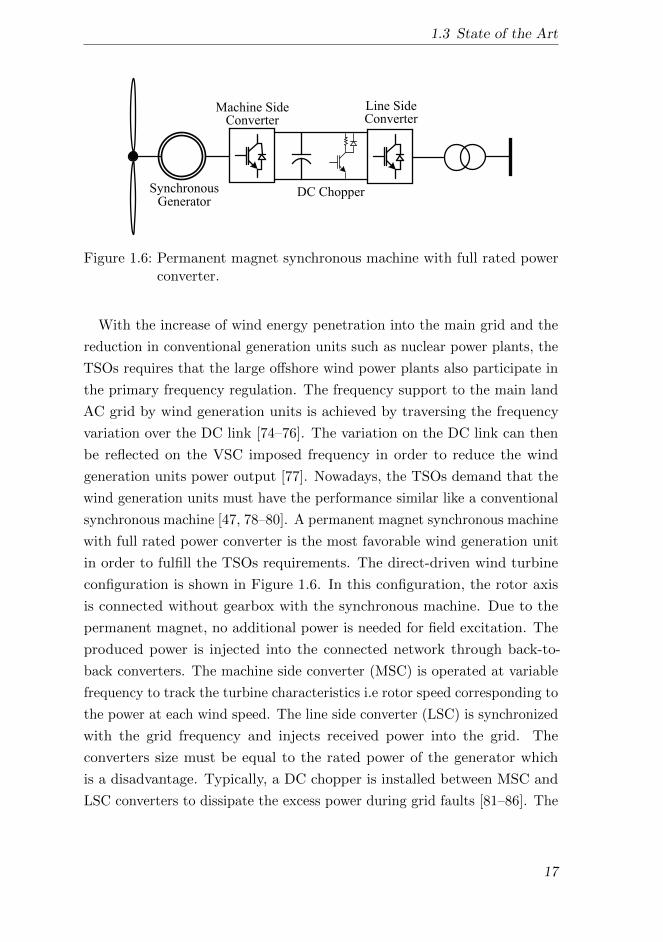
1.6 Permanent magnet synchronous machine with full ratedpower converter. . . . . . . . . . . . . . . . . . . . . . . . . 17

2.1 MIMO structures of two input two output system. . . . . . 24

2.2 Axis transformation from abc to dq0 frame. . . . . . . . . . 26

2.3 MMC VSC converter and an equivalent averaged model. . 29

2.4 Voltage source converter substation configuration. . . . . . 30

2.5 Overview of cascaded voltage source converter control. . . 31

2.6 Phase-locked loop control system for converter grid syn-chronization. . . . . . . . . . . . . . . . . . . . . . . . . . . 32

2.7 Converter current open loop model. . . . . . . . . . . . . . 34

2.8 A generalized closed loop control structure including statedecoupling scheme. . . . . . . . . . . . . . . . . . . . . . . 35

2.9 Open loop current model including decoupling scheme. . . 36

2.10 Closed loop feedback control system for current. . . . . . . 37

2.11 Root locus analysis of closed loop current control of theVSC HVDC system. . . . . . . . . . . . . . . . . . . . . . . 38

2.12 Under-damped performance analysis of the closed loop cur-rent control. . . . . . . . . . . . . . . . . . . . . . . . . . . 39

2.13 Bode plot for analyzing parametric sensitivity of VSC cur-rent closed loop control. . . . . . . . . . . . . . . . . . . . . 41

2.14 Current step response analysis for system sensitivity anddecoupled scheme verification. . . . . . . . . . . . . . . . . 42

xvii

List of Figures

2.15 Grid connected VSC open loop control block diagram withrespect to the outer controller. . . . . . . . . . . . . . . . . 43

2.16 Closed loop feedback diagram for power controller designin grid synchronous mode. . . . . . . . . . . . . . . . . . . 46

2.17 Active and reactive power control analysis of VSC in gridsynchronous mode. . . . . . . . . . . . . . . . . . . . . . . . 47

2.18 Closed loop block diagram of VSC DC voltage control. . . 48

2.19 Frequency response analysis and nonlinear time domainsimulation results of VSC DC voltage control. . . . . . . . 49

2.20 AC voltage nonlinear control implementation of VSC ingrid synchronous mode. . . . . . . . . . . . . . . . . . . . . 50

2.21 Dynamic and stability analysis of VSC AC voltage controlin grid synchronous mode. . . . . . . . . . . . . . . . . . . 51

2.22 Block diagram of voltage d− and q− component decouplingfor grid forming control. . . . . . . . . . . . . . . . . . . . . 53

2.23 VSC Closed loop block diagram of grid forming control. . . 54

2.24 Bode analysis of VSC grid forming voltage control. . . . . . 55

2.25 Nonlinear simulation results of VSC grid forming voltagecontrol. . . . . . . . . . . . . . . . . . . . . . . . . . . . . . 56

2.26 Offshore substation configuration of VSC HVDC transmis-sion system. . . . . . . . . . . . . . . . . . . . . . . . . . . 57

2.27 Onshore substation configuration of VSC HVDC transmis-sion system. . . . . . . . . . . . . . . . . . . . . . . . . . . 59

2.28 Grid side wind turbine VSC substation configuration. . . . 61

3.1 Configuration of an offshore AC network to integrate windpower plants using VSC HVDC transmission system withseveral onshore grids. . . . . . . . . . . . . . . . . . . . . . 65

3.2 The grid forming control of the offshore converter for paralleloperation of VSC HVDC transmission systems. . . . . . . . 66

3.3 Comparison of active power sharing techniques. . . . . . . 68

3.4 Illustration of frequency and active power distribution usingset-points. . . . . . . . . . . . . . . . . . . . . . . . . . . . 69

3.5 Illustration of frequency response and active power distri-bution using droop gains of an offshore AC network. . . . . 71

3.6 An impedance diagram of an offshore AC network for powerflow analysis. . . . . . . . . . . . . . . . . . . . . . . . . . . 72

3.7 The comparison of VSC power flow response with andwithout droop scheme. . . . . . . . . . . . . . . . . . . . . 74

xviii

List of Figures

3.8 Illustration of the frequency and voltage droop effects onthe VSC power flow. . . . . . . . . . . . . . . . . . . . . . . 80

3.9 Nonlinear simulation result of offshore AC network havingmultiple grid forming VSC HVDC transmission system. . . 82

3.10 The response of voltage d -component of the VSCs control-ling busbars. . . . . . . . . . . . . . . . . . . . . . . . . . . 83

3.11 Configuration of an offshore AC network interconnectingtwo onshore grid using VSC HVDC transmission system. . 84

3.12 Total active power losses of the system. . . . . . . . . . . . 92

3.13 Wind profile according to the FINO 1, 2, and 3 database,and ENERCON wind turbine power curve. . . . . . . . . . 93

3.14 Pareto Front analysis of objective functions with respect toobjective weighting factor (γ). . . . . . . . . . . . . . . . . 94

3.15 Offshore grid busbars voltage probability at the given γ andα. . . . . . . . . . . . . . . . . . . . . . . . . . . . . . . . . 95

3.16 The response of reactive power sharing with respect to αand γ. . . . . . . . . . . . . . . . . . . . . . . . . . . . . . . 96

3.17 The responses of active power loss comparison with andwithout voltage droop control, and the frequencies at α =0.3 and γ = 1.0. . . . . . . . . . . . . . . . . . . . . . . . . 97

3.18 Comparison of the reactive power support by wind powerplants at α = 0.3, and γ = 1.0 with and without voltagedroop control. . . . . . . . . . . . . . . . . . . . . . . . . . 98

3.19 Comparison of the reactive power support by VSC-HVDCsystem at α = 0.3, and γ = 1.0 with and without voltagedroop control. . . . . . . . . . . . . . . . . . . . . . . . . . 99

4.1 An overview of an offshore AC network interconnectingseveral offshore wind power plants with different onshoregrids. . . . . . . . . . . . . . . . . . . . . . . . . . . . . . . 104

4.2 Grid forming voltage source converter control system foran offshore AC network. . . . . . . . . . . . . . . . . . . . . 105

4.3 An open loop block diagram of an offshore AC networksmall signal model in the state space representation. . . . . 107

4.4 Illustration of VSC variables transformation into commonreference frame. . . . . . . . . . . . . . . . . . . . . . . . . 110

4.5 A simplified diagram for modeling offshore AC networkbranches and busbars. . . . . . . . . . . . . . . . . . . . . . 114

4.6 Offshore AC network having two frequency controlled voltagesource converter. . . . . . . . . . . . . . . . . . . . . . . . . 116

xix

List of Figures

4.7 Poles-Zeros map of offshore AC network having multiplegrid forming VSCs. . . . . . . . . . . . . . . . . . . . . . . 124

4.8 Poles maps of the offshore AC network with or withoutincluding low-pass filter on power measurements. . . . . . . 125

4.9 The nonlinear time domain simulation plots of converterscontrolling busbar. . . . . . . . . . . . . . . . . . . . . . . . 126

4.10 The frequency response analysis of the VSC-1 output voltageand the network frequency change with respect of windactive current. . . . . . . . . . . . . . . . . . . . . . . . . . 127

4.11 Power response of the VSCs without having low pass filtersat the power measurements. . . . . . . . . . . . . . . . . . 128

4.12 Power response of the VSCs having low pass filters at thepower measurements. . . . . . . . . . . . . . . . . . . . . . 129

4.13 Nonlinear simulation response of VSCs frequencies. . . . . 130

4.14 A nonlinear simulation test for the validation of stabilityrange and sensitivity analysis. . . . . . . . . . . . . . . . . 131

5.1 Configuration of offshore AC network integrating two on-shore grids with three wind power plants using VSC HVDCtransmission system in point to point configuration. . . . . 135

5.2 Control system of wind generation units including shortcircuit scheme. . . . . . . . . . . . . . . . . . . . . . . . . . 137

5.3 The outer voltage control of wind generation unit. . . . . . 138

5.4 Offshore VSC control for HVDC system including shortcircuit scheme. . . . . . . . . . . . . . . . . . . . . . . . . . 139

5.5 Onshore VSC control for HVDC system including shortcircuit scheme. . . . . . . . . . . . . . . . . . . . . . . . . . 140

5.6 An equivalent impedance diagram of voltage source conver-ter substation to analyze PQ characteristic. . . . . . . . . . 141

5.7 PQ characteristic analysis of VSC HVDC substation todetermine voltage and current operational limits. . . . . . . 142

5.8 Simplified offshore AC network diagram for short circuitanalysis. . . . . . . . . . . . . . . . . . . . . . . . . . . . . 144

5.9 Effect of fault impedance magnitude on busbar voltages. . 145

5.10 Offshore network voltages level in polar coordinates. . . . . 147

5.11 Offshore network voltages with and without wind powerplant current infeed. . . . . . . . . . . . . . . . . . . . . . . 148

5.12 The over limit current control of HVDC transmission systemoffshore side voltage source converter. . . . . . . . . . . . . 151

xx

List of Figures

5.13 Frequency control power limit with droop control for off-shore VSC HVDC system. . . . . . . . . . . . . . . . . . . 152

5.14 Voltage support control scheme of wind generation units. . 153

5.15 Chopper control scheme to control DC link of wind genera-tion unit during fault. . . . . . . . . . . . . . . . . . . . . . 154

5.16 Voltage and frequency dependent active current reductionscheme of wind generation unit. . . . . . . . . . . . . . . . 155

5.17 Short circuit response of VSC 1 and 2 substation currentsand voltages for fault at 33kV wind turbine busbar. . . . . 159

5.18 VSC 1 and 2 substation voltage phase angles for fault at33kV wind turbine busbar. . . . . . . . . . . . . . . . . . . 160

5.19 Voltage short circuit response of 150kV busbar fault. . . . 161

5.20 Frequency and current short circuit response of 150kVHVAC cable fault. . . . . . . . . . . . . . . . . . . . . . . . 162

5.21 Response of the offshore AC network in the event of VSC 2substation disconnection. . . . . . . . . . . . . . . . . . . . 164

5.22 The network short circuit voltage and current response ofthe fault applied at country A onshore grid. . . . . . . . . 165

6.1 Offshore AC and DC grid interconnection with the onshoregrids. . . . . . . . . . . . . . . . . . . . . . . . . . . . . . . 168

6.2 The characteristic curve of master-slave and voltage margincontrol principle. . . . . . . . . . . . . . . . . . . . . . . . . 169

6.3 Onshore VSC substation and its control scheme for MTDCnetwork. . . . . . . . . . . . . . . . . . . . . . . . . . . . . 170

6.4 U-I characteristic of onshore VSCs DC voltage control tooperate MTDC network. . . . . . . . . . . . . . . . . . . . 172

6.5 Offshore multiterminal HVDC network. . . . . . . . . . . . 175

6.6 DC current and voltage responses of the MTDC system atα1 = α2 = 0.33, and α3 = 0.34. . . . . . . . . . . . . . . . . 177

6.7 DC current and voltage responses of the MTDC networkat α1 = α2 = 0.5, and α3 = 0.0. . . . . . . . . . . . . . . . 178

6.8 DC current and voltage response of the MTDC system atα1 = 0.1, α2 = 0.3, and α3 = 0.6. . . . . . . . . . . . . . . . 179

6.9 The dead-band droop characteristic and its control system. 180

6.10 DC current and voltage response of the MTDC system withdead-band droop control. . . . . . . . . . . . . . . . . . . . 181

6.11 Integration of offshore AC and DC networks. . . . . . . . . 183

6.12 The power response of offshore VSCs. . . . . . . . . . . . . 185

xxi

List of Figures

6.13 The response of offshore VSCs frequencies and their corre-sponding busbar voltages. . . . . . . . . . . . . . . . . . . . 186

6.14 The active power and DC voltage response of the onshoreconverters. . . . . . . . . . . . . . . . . . . . . . . . . . . . 187

xxii

List of Tables

1.1 Salient feature of voltage source and line commutated con-verter based HVDC transmission system . . . . . . . . . . 8

1.2 List of VSC based HVDC system projects . . . . . . . . . . 10

2.1 Offshore VSC HVDC substation network and control para-meters . . . . . . . . . . . . . . . . . . . . . . . . . . . . . . 58

2.2 Onshore VSC HVDC substation network and control para-meters . . . . . . . . . . . . . . . . . . . . . . . . . . . . . . 60

2.3 Wind generation unit network and control parameters . . . 62

3.1 Offshore AC network impedances for power flow analysis . 733.2 Droop gain values according to proposed method . . . . . . 793.3 Offshore AC network impedances for OPF algorithm . . . 85

4.1 Offshore AC network and control parameters for stabilityanalysis . . . . . . . . . . . . . . . . . . . . . . . . . . . . . 117

5.1 Cables and transformer parameters . . . . . . . . . . . . . 136

6.1 MTDC network operational scenarios and voltage controllergains . . . . . . . . . . . . . . . . . . . . . . . . . . . . . . 176

6.2 Network voltages and cables parameters for combined ACand DC grid . . . . . . . . . . . . . . . . . . . . . . . . . . 184

xxiii

xxiv

1 Introduction

This chapter explains the background of the thesis and the challenges that

future offshore wind power integration may face. The aim and contribution

of the thesis are also described in this chapter.

1.1 The Emergence of Offshore Wind Energy

The current era requires attention to unprecedented issues of security and

sustainability of energy generation. A threat of global warming is also added

in the existing challenges of diminishing fossil resources and increasing world

population [1]. The world must escape from the dependency of pollutant

technologies of energy generation, and move towards a clean and sustainable

source of generation to meet the future energy demand [2].

Renewable resources have made the biggest transition in the global energy

sector compared to fossil fuels. Among all the new power generation in-

stallation in EU in 2015, the share of renewable energy is 77 % whereas

more energy was from conventional power sources decommission compare

to their new install [3]. In Europe alone, 224 GW of renewables was added

over the last decade, of which 122 GW is produced by new installation of

wind power plants during 2005-2016 [3, 4]. Whereas, every year generation

from fossil fuels is reduced with an average of 10 GW installed capacity

[3]. Wind energy is the fastest growing technology among other renewables.

In 2016, wind energy with the capacity of 12.5 GW was installed in the

European Union which amounts to 51 % of all new installation [4]. Of

the total installed capacity in 2016, 10.923 GW was installed onshore and

1.567 GW offshore [4]. The annual growth of onshore and offshore wind

power is shown in Figure 1.1. By the end of 2016, the EU-28 countries

installed 153.7 GW wind power capacity, out of which 141.1 GW is onshore

1

1 Introduction

0.0

2.0

4.0

6.0

8.0

10.0

12.0

14.0

2005 2006 2007 2008 2009 2010 2011 2012 2013 2014 2015 2016

Po

wer

(G

W)

Years

Source: WindEuropeOnshore Offshore

Figure 1.1: Annual onshore and offshore wind power in the EU.

and 12.6 GW offshore. Germany is the leading country with the highest

number of installed wind power capacity, followed by Spain, UK, and France

[4]. During 2016, Germany has installed four wind power plants having total

number of 155 fully grid connected wind turbines with the total installed

power of 813 MW [5]. Until now, Germany has installed up to 50.0 GW of

cumulative onshore and offshore wind energy. Whereas, Spain has 23.1 GW

and UK has 14.5 GW of cumulative installed wind energy. This trend of

connecting wind energy into European grid will be continued in order to

achieved the target of EU 2030 climate and energy framework. The frame-

work set three main targets i.e reduction in greenhouse gas emissions up to

40 % since 1990 level, increase in renewable energy share of at least 27 %

of EU energy consumption, and at least 27 % improvement in the energy

efficiency [6].

Wind industry has emerged as a proven technology for the clean and

affordable energy in order to fulfill the ambitious energy policies of EU.

The wind energy resources are huge in Europe. However, the cost-effective

development is the key challenge. Onshore, high wind energy potential

is available in the industrial and agricultural areas. The environmental

and social constraints associated with land acquisition for onshore wind

power plant development are the main limiting factors in utilizing the wind

potential to its full extent. Also, the environmental and social constraints

such as Natura 2000 areas, shipping lane, and military areas leave up to

2

1.1 The Emergence of Offshore Wind Energy

4 % of offshore area within the 10 km of the EEA countries coast to build

wind power plants. This has reduced the offshore wind utilization potential

by more than 85 % of total available wind power near coast (2800 TWh

of 25000 TWh in 2020) [7]. These onshore and near to coast limitations

for wind power plants installation are forcing to go deeper into the Sea.

As illustrated in Figure 1.2, many offshore wind power plants are under

construction and consented for future installation far from the shore [8].

Future wind power plants are expected to be installed as far as 100 km and as

deep as 50 m. Around, 100 GW of offshore wind energy projects have already

been proposed in North and Baltic Sea. The grid integration of such huge

offshore energy requires an unique infrastructure. European Wind Energy

Association (EWEA) have proposed a 20 year offshore network development

plan which provides gradual approach to plan offshore grid in the North

and Baltic Seas. The future offshore grid will not only be a national grid

but it will become an European backbone for electricity trade. The future

transnational offshore grid will provide benefit to European countries such

as access to offshore wind energy, enhance the ability to trade electricity,

and smooth the wind energy variability in the markets [9]. The concept

of integrated network is not limited to Europe only but it is being given

importance worldwide [10]. Some of the initiatives that are taken worldwide

to construct international electrical grid are list below:

• Friends of SuperGrid: The Friends of Supergrid (FOSG) is a group

of companies and organizations who are promoting the concept of

Supergrid in Europe. According to them a SuperGrid is ‘a pan-

European transmission network facilitating the integration of large-

scale renewable energy and the balancing and the transportation of

electricity’. The FOSG proposed the SuperGrid technology roadmap

that provides a comprehensive overview on the energy transmission

technology evolution for interconnections between European countries

until 2050. The roadmap also propose EU level regulatory framework

which will accelerate the Supergrid projects.

• Offshore Grid: It is an European project which will set the offshore

grid regulatory framework considering economic, technical, policy and

3

1 Introduction

Source: WindEurope

Dis

tance

to s

hore

(km

)

Average Water depth (m)

Online

UnderConstruction

Consented 0

20

40

60

80

100

120

10 20 30 40 50

Figure 1.2: Average water depth and distance to shore of offshore wind powerplants (bubble size indicates the installed size).

regulatory aspects. In the first phase, the project focuses on the regions

of North Sea, Baltic Sea, the English Channel, and the Irish Sea. In

the second phase, the results will be applied for the Mediterranean

projects.

• Atlantic Wind Connection: This project will construct an offshore

electrical transmission system around the mid-Atlantic region. It will

be built in three phases over the period of ten years. In the first

phase, New Jersey Energy Link will be built which will connect the

South Jersey electrical network with North Jersey electrical grid. The

DelMARVA Energ Link will be built in the second phase in which wind

power plants more than 16.1 km off the coast of Delaware, Maryland

and Virginia will create three offshore hubs to connect with the onshore

grids. In the third phase, the Bay Link will be developed that will

complete the interconnection between the New Jersey Energy Link and

the Delmarva Energy Link forming the north-south offshore backbone.

• Medgrid: It is an Euro-Mediterranean electricity network planned to

build for providing inexpensive renewable electricity in North Africa

4

1.1 The Emergence of Offshore Wind Energy

AC Hub

DC Hub

HVDC Cable

HVAC Cable

Offshore

Onshore

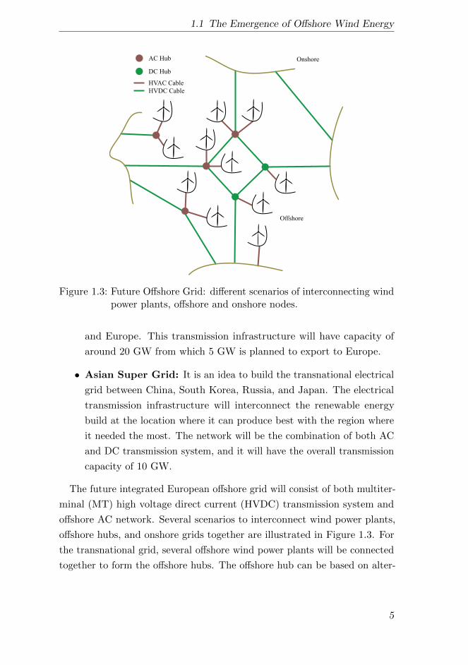
Figure 1.3: Future Offshore Grid: different scenarios of interconnecting windpower plants, offshore and onshore nodes.

and Europe. This transmission infrastructure will have capacity of

around 20 GW from which 5 GW is planned to export to Europe.

• Asian Super Grid: It is an idea to build the transnational electrical

grid between China, South Korea, Russia, and Japan. The electrical

transmission infrastructure will interconnect the renewable energy

build at the location where it can produce best with the region where

it needed the most. The network will be the combination of both AC

and DC transmission system, and it will have the overall transmission

capacity of 10 GW.

The future integrated European offshore grid will consist of both multiter-

minal (MT) high voltage direct current (HVDC) transmission system and

offshore AC network. Several scenarios to interconnect wind power plants,

offshore hubs, and onshore grids together are illustrated in Figure 1.3. For

the transnational grid, several offshore wind power plants will be connected

together to form the offshore hubs. The offshore hub can be based on alter-

5

1 Introduction

nating current (AC) and/or direct current (DC) technology. These offshore

hubs will act as the mediator between wind power plants and different coun-

tries. The net power from these hubs will be transferred where it is needed

hereby enhances trade and improves competition in the European energy

market. This will improve the connection between load centers around the

North and Baltic Sea, and develop more interconnection between countries

which avoid the bottleneck on the existing international inter-connectors [11].

Although the transactional grid have several economical benefits, it requires

further research to address technical challenges associated with it. Such as

what is the control and operational principle of an offshore AC or DC hub;

how to ensure the offshore grid stability; how power is distributed through

the AC or DC hub; what would be the behavior of the wind turbines and

transmission system during short circuit at offshore grid etc. In this context,

this thesis focus on the following key points:

• Control and operation of the HVDC transmission system for offshore

hubs

• Control of the active and reactive power flow within the offshore grids

• Integration of the offshore AC and DC hubs

1.2 MEDOW: A Solution to Global Warming

The threat of global warming has risen to an alarming level in last two

decades. There is an urgent need of reducing greenhouses gases, such as

carbon dioxide, to restrain the fast changes of climate. The energy generation

by burning fossil fuels, such as coal, oil, and natural gas, has highest impact

on the atmosphere than any other human activity. Globally, power generation

is adding almost 700 tonnes of CO2 emission every second and 23 billion

tonnes every year [12]. To reduce climate risks, the CO2 emissions must be

cut by deploying green power sources like wind energy. European Union (EU)

has taken several steps toward the clean energy generation prominently from

wind. Many research projects are ongoing to study the feasibility of wind

generation and its integration with the existing grid especially for offshore

6

1.3 State of the Art

wind power plants. One of these project is MEDOW: Multi-tErminal Dc

grid for Offshore Wind [13].

MEDOW is a Marie Curie Initial Training Network (ITN) which consists of

five universities and six industrial organizations. The objective of the project

is to find the solutions to the issues of offshore grid for integrating wind energy.

The overall objectives of the project are divided into four work packages (WP)

i.e connection of offshore wind power to DC grids (WP-1), investigation of

voltage source converters for DC grids (WP- 2), relaying protection (WP-3),

and interactive AC/DC grids (WP-4). The achievements from the project

will contribute in the technological development for integrating offshore

wind power with the onshore grids in European countries. The project has

suggested that the DC grid will be the key technology in realizing the future

European offshore ‘SuperGrid’. In addition, the project has also offered a

development path to researchers across Europe in the area of DC grids.

The presented thesis is the part of the MEDOW research work. The

thesis has contributed to achieve the following milestones and deliverables

of WP-1:

• Design of converter control and its operational mode characteristics.

• Evaluation of AC and DC grid configuration for offshore wind power

plants.

• Development of optimum power flow algorithm for offshore grids.

• Method of reducing wind power during disturbance.

During the execution of the thesis, the collaboration with MEDOW

partners have been done on varies aspect of the thesis research area.

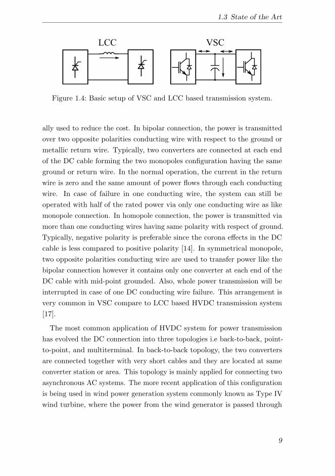
1.3 State of the Art

A voltage source converter (VSC) based high voltage direct current (HVDC)

transmission system is getting preference over line commutated converter

(LCC) based HVDC transmission system due to its operational principle.

Although the LCC technology is well developed and available for high power

7

1 Introduction

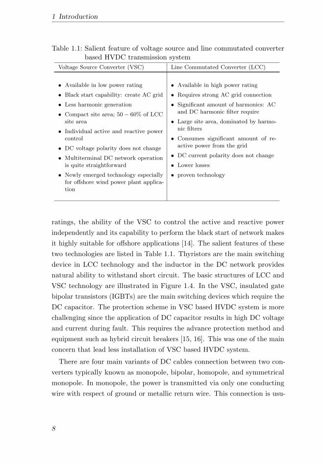
Table 1.1: Salient feature of voltage source and line commutated converterbased HVDC transmission system

Voltage Source Converter (VSC) Line Commutated Converter (LCC)

• Available in low power rating

• Black start capability: create AC grid

• Less harmonic generation

• Compact site area; 50 − 60% of LCCsite area

• Individual active and reactive powercontrol

• DC voltage polarity does not change

• Multiterminal DC network operationis quite straightforward

• Newly emerged technology especiallyfor offshore wind power plant applica-tion

• Available in high power rating

• Requires strong AC grid connection

• Significant amount of harmonics: ACand DC harmonic filter require

• Large site area, dominated by harmo-nic filters

• Consumes significant amount of re-active power from the grid

• DC current polarity does not change

• Lower losses

• proven technology

ratings, the ability of the VSC to control the active and reactive power

independently and its capability to perform the black start of network makes

it highly suitable for offshore applications [14]. The salient features of these

two technologies are listed in Table 1.1. Thyristors are the main switching

device in LCC technology and the inductor in the DC network provides

natural ability to withstand short circuit. The basic structures of LCC and

VSC technology are illustrated in Figure 1.4. In the VSC, insulated gate

bipolar transistors (IGBTs) are the main switching devices which require the

DC capacitor. The protection scheme in VSC based HVDC system is more

challenging since the application of DC capacitor results in high DC voltage

and current during fault. This requires the advance protection method and

equipment such as hybrid circuit breakers [15, 16]. This was one of the main

concern that lead less installation of VSC based HVDC system.

There are four main variants of DC cables connection between two con-

verters typically known as monopole, bipolar, homopole, and symmetrical

monopole. In monopole, the power is transmitted via only one conducting

wire with respect of ground or metallic return wire. This connection is usu-

8

1.3 State of the Art

VSCLCC

Figure 1.4: Basic setup of VSC and LCC based transmission system.

ally used to reduce the cost. In bipolar connection, the power is transmitted

over two opposite polarities conducting wire with respect to the ground or

metallic return wire. Typically, two converters are connected at each end

of the DC cable forming the two monopoles configuration having the same

ground or return wire. In the normal operation, the current in the return

wire is zero and the same amount of power flows through each conducting

wire. In case of failure in one conducting wire, the system can still be

operated with half of the rated power via only one conducting wire as like

monopole connection. In homopole connection, the power is transmitted via

more than one conducting wires having same polarity with respect of ground.

Typically, negative polarity is preferable since the corona effects in the DC

cable is less compared to positive polarity [14]. In symmetrical monopole,

two opposite polarities conducting wire are used to transfer power like the

bipolar connection however it contains only one converter at each end of the

DC cable with mid-point grounded. Also, whole power transmission will be

interrupted in case of one DC conducting wire failure. This arrangement is

very common in VSC compare to LCC based HVDC transmission system

[17].

The most common application of HVDC system for power transmission

has evolved the DC connection into three topologies i.e back-to-back, point-

to-point, and multiterminal. In back-to-back topology, the two converters

are connected together with very short cables and they are located at same

converter station or area. This topology is mainly applied for connecting two

asynchronous AC systems. The more recent application of this configuration

is being used in wind power generation system commonly known as Type IV

wind turbine, where the power from the wind generator is passed through

9

1 Introduction

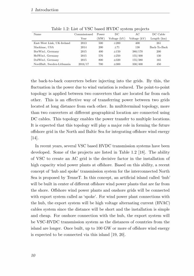
Table 1.2: List of VSC based HVDC system projectsName Commissioned Power DC AC DC Cable

Year (MW) Voltage (kV) Voltage (kV) Length (km)

East-West Link, UK-Ireland 2013 500 ±200 400 261

Mackinac, USA 2014 200 ±71 138 Back-To-Back

BorWin1, Germany 2015 400 ±150 380/170 200

HelWin1, Germany 2015 576 ±250 155/400 130

DolWin1, Germany 2015 800 ±320 155/380 165

NordBalt, Sweden-Lithuania 2016/17 700 ±300 330/400 450

the back-to-back converters before injecting into the grids. By this, the

fluctuation in the power due to wind variation is reduced. The point-to-point

topology is applied between two converters that are located far from each

other. This is an effective way of transferring power between two grids

located at long distance from each other. In multiterminal topology, more

than two converters at different geographical location are connected using

DC cables. This topology enables the power transfer to multiple locations.

It is expected that this topology will play a major role in forming the future

offshore grid in the North and Baltic Sea for integrating offshore wind energy

[14].

In recent years, several VSC based HVDC transmission systems have been

developed. Some of the projects are listed in Table 1.2 [18]. The ability

of VSC to create an AC grid is the decisive factor in the installation of

high capacity wind power plants at offshore. Based on this ability, a recent

concept of ‘hub and spoke’ transmission system for the interconnected North

Sea is proposed by TenneT. In this concept, an artificial island called ‘hub’

will be built in center of different offshore wind power plants that are far from

the shore. Offshore wind power plants and onshore grids will be connected

with export system called as ‘spoke’. For wind power plant connections with

the hub, the export system will be high voltage alternating current (HVAC)

cables system since the distance will be short and the installation is simple

and cheap. For onshore connection with the hub, the export system will

be VSC-HVDC transmission system as the distances of countries from the

island are longer. Once built, up to 100 GW or more of offshore wind energy

is expected to be connected via this island [19, 20].

10

1.3 State of the Art

AC Platform

HVDC Plateform

HVAC Cables

MVAC Cables

HVDC Cables

(a)

AC Platform

HVDC Plateform

HVAC Cables

MVAC Cables

HVAC Cables

HVDC Cables

(b)

AC Platform

HVDC Plateform

HVAC Cables

MVAC Cables

HVDC Cables

HVAC

Interconnection

(c)

AC Platform

HVDC Plateform

HVAC Cables

MVAC Cables

HVDC CablesHVDC

Interconnection

(d)

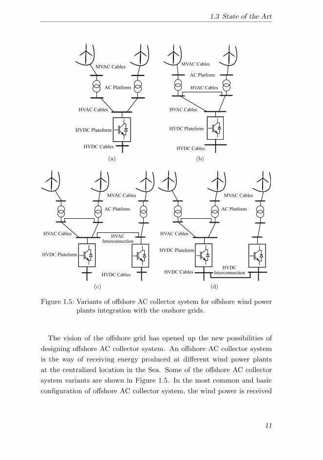
Figure 1.5: Variants of offshore AC collector system for offshore wind powerplants integration with the onshore grids.

The vision of the offshore grid has opened up the new possibilities of

designing offshore AC collector system. An offshore AC collector system

is the way of receiving energy produced at different wind power plants

at the centralized location in the Sea. Some of the offshore AC collector

system variants are shown in Figure 1.5. In the most common and basic

configuration of offshore AC collector system, the wind power is received

11

1 Introduction

at the offshore AC platform using MVAC cables. Typically, these MVAC

cables are the arrays of offshore wind power plant in radial or radial-ring

configuration. The offshore AC platform is then connected to an offshore

HVDC platform via HVAC cables, there the collected power is transferred to

the onshore grid using HVDC transmission system. The number of offshore

AC platforms depends on the wind power plant layout and capacity [21].

These AC platforms can belong to the same or different wind power plants.

By this, combined energy from wind power plants that are far from shore can

be transferred economically via single HVDC transmission system. In order

to increase the redundancy in the AC network, the offshore AC platforms

can be connected together as well using HVAC cable. Normally, the voltage

of the cables in the wind power plant array is in the range of 30− 36 kV.

And the HVAC cables have the typical voltage rating of 132, 150 or 220 kV.

The number of interconnected offshore wind power plants are limited by

the total power transfer capability of the offshore converter, also the power

is only transmitted to a single onshore grid in this configuration. In order

to increase the trade and overall capability of energy export, more than

one HVDC platform can be built and interconnected with each other either

using HVAC or HVDC cable depending on distance between them [22].

Nowadays, the export system between onshore grid and offshore wind

power plant is the main focus of the transmission system operators (TSOs).

Although the studies have highlighted the advantages of HVDC transmission

system over HVAC system, there are more offshore wind power plants

currently installed at North Sea using HVAC cables. This is due to the

simple installation procedure and the vast experience of the industries with it.

The reactive power flow through the offshore HVAC cables is the main barrier

in applying this technology for high capacity wind power plants, especially

for long distance [23]. The reactive power compensation increases the overall

cost of the system. The HVAC export system is usually applied for offshore

wind power plant distance less than 60 km from shore [24]. In literature,

there are some suggestion to use the non-standard frequencies to reduce the

over all cost of the system [25–27]. At higher frequencies, the size of the

transformer significantly reduces however the number of cable connections

increases as well as the cables charging current for longer distance. Lower

12

1.3 State of the Art

frequencies, such as 16.7 Hz, enable the high power transmission over long

distance. This may reduce the total number of cables and compensation

equipments. But, the low frequency AC (LFAC) system produces more

oscillation in the voltage transient, increased amount of low order harmonics,

increase in transformer cost, and high short circuit current in the network.

The feasibility study of using the non-standard frequencies for the offshore

network is at preliminary level, and it particularly requires a mechanism

to integrate existing offshore infrastructure with the future developments

to encompass the ‘SuperGrid’ concept. On the other hand, VSC based

multiterminal HVDC transmission systems provide more features and ease

in operational control such as control of power flow direction in the DC

network, independent active and reactive power control in the AC network,

frequency support etc.

With the introduction of modular multi-level converter (MMC) technology,

the overall system efficiency vs cost has been increased. The MMC generates

the AC output signal in hundreds of small steps and contain low harmonics

contents hereby require fewer AC filters. Due to the control structure of

MMC, all the semiconductors are not switched simultaneously and the

average switching frequency is between 100 to 200 HZ. This has reduced

the total converter losses down to 1 % [28]. Moreover, the converter is

designed in modular way which means that each arm is constructed by

connecting individual sub-modules in series. Each sub-module contains its

own DC capacitor which eliminates the need of additional DC capacitor at

the DC link. The output voltage level is then the function of the number of

sub-modules in each arm. By this design, the power rating of the converter

can just be increased by increasing the stack of the sub-modules [29–31].

With the increase of power electronics devices such as VSCs in the network,

the inertia in the system is reduced which affects the overall system dynamics,

and the VSCs must also ensure the system stability [32]. The interaction of

VSC with network for offshore wind power plant integration is happened

at three levels i.e at onshore grid connection point, in the DC network,

and in the offshore AC network. Typically, the VSC connected with the

onshore network is synchronized with grid frequency and controls the power

flow either by direct or vector control method [33]. The direct control

13

1 Introduction

method does not have the current limiting capability and its bandwidth is

limited due to AC resonance frequencies. On the other hand, the vector

control manipulates the current to control the power flow in the rotating

reference frame. The vector control method enables the decouple control

of active and reactive power flow, however the transformation of signals

into dq0 rotating frame introduces the 2ω cross-couple oscillation produced

by positive and negative sequence current injection under unbalanced grid

voltage condition [34]. This oscillation can be damped by employing active

and passive filtration methods [35–38]. There are different variants of passive

filters such as L, LC, LCL etc. Passive filter are required particularly in two

or three level PWM converters [39–42]. It is suggested that the LCL filter

are more cost-effective compared to L-filters since a smaller inductor can be

applied to achieve the same reduction in the switching harmonics [43]. For

MMC based converter, a simple L-filter can provide the necessary harmonic

reduction in the system.

Usually, onshore grids are operated at their maximum level to fully utilized

infrastructure. In this situation, the transient behavior of the system has

uttermost importance in order to prevent operational limits violations and

instability. The TSOs define the required characteristics in their grid codes for

the generation units (for example VSCs and wind turbines), which includes

both short circuit and normal operation such as voltage support, fault-ride

through, frequency support etc [44–46]. Among the grid code requirements,

fault-ride through (FRT) is the most critical and important requirement that

need to be fulfilled at the point of common coupling (PCC). In FRT support,

it is required that the generation units must not be disconnected after few

millisecond (approximately 150 ms) during a fault [47, 48]. In VSCs, such

a characteristic is achieved by employing a DC chopper [49]. During fault

period, the power is dissipated through DC chopper to maintain the DC

voltage within the operational limits. Furthermore, VSCs are required to

inject only reactive current to support the grid voltage during grid fault.

The stability of the DC network highly depends on the control of the

DC voltage [50]. In the VSC-HVDC system for integrating offshore wind

energy, the onshore converter has the main responsibility to control the

DC voltage regardless whether the DC network is a point-to-point link or

14

1.3 State of the Art

MTDC. In the point-to-point configuration, the onshore converter has the

sole responsibility to maintain the DC voltage which is typically achieved

by applying proportional-plus-integral (PI) control system [51]. For the

MTDC network, there are several voltage control strategies proposed in

the literature such as centralized DC slack bus control, voltage margin

control, and distributed voltage droop control [52]. Using droop control,

the responsibility to balance the DC voltage is distributed among several

onshore VSC in the MTDC system without communication signals. The

voltage droop control provide robust performance as well as power sharing

among converters [53, 54]. The voltage droop control is either based on

current or power feedback signal. The distribution of the net power in a

MTDC network among converters can be made by selecting appropriate

droop slopes, however the droop characteristic increases the complexity in

power flow. The power infeed into the onshore AC grids are of fluctuating

nature due to wind power variation. Furthermore, it is difficult to steer

power between converters with droop schemes. In order to compensate

these limitations, the enhancements in the droop control scheme have been

proposed such as dead-band droop control, ratio control, priority control etc

[55–58]. Generally, the control of the DC network regulate the DC voltage

that varies the power flows in the cables. Although the power losses in the

DC cable is less than the AC cable, an optimal power flow (OPF) algorithm

of the combined AC and DC network is required to achieve the desire steady-

state operating points [59–62]. Additionally, the OPF algorithm provides

the control parameters considering criteria such as minimizing losses, cost

function, voltage deviation etc.

The protection of the MTDC network is one of the important issue

nowadays [63, 64]. The DC circuit breaker is still a new technology which has

relatively high cost. There are several types of DC circuit break technologies

exist such as mechanical circuit breaker with passive or active resonance

circuit, hybrid technology which is the combination of mechanical and

controllable solid-state devices, and pure solid-state circuit breaker. The

performance of the DC circuit breaker is related to its interruption time,

power losses, and availability in different voltage and current rating. The DC

fault requires fast interruption time compared to AC fault. The mechanical

15

1 Introduction

circuit breaker can interrupt up to 60 ms whereas pure semiconductor based

circuit breaker interruption time can be achieved less than 1.0 ms. The

mechanical circuit breaker has the lowest power losses due to lower voltage

drop across the metallic contact of the main circuit breaker connected in

the normal conduction path. The power loss during normal operation is less

than 0.001 % in the mechanical circuit breaker, and the power loss up to

0.1 % may occur in the hybrid circuit breaker. Pure semiconductor based

circuit breaker has the highest power loss due to the presence of several

switching devices in the main current conduction path. The mechanical

circuit breaker is available in high voltage and current rating i.e up to 550 kV

and 8.0 kA. The hybrid circuit breaker has comparatively lower voltage

rating i.e 120 kV. However, its theoretical current rating can goes up to 16 kA.

Pure semiconductor circuit breakers are mainly available for medium voltage

level applications. The DC network protection scheme greatly depends on

the MTDC topologies (such as ring, star, star with central switching ring,

wind power plant ring, substation ring) based on the criteria of redundancy,

flexibility and need of communication [16, 65].

The offshore AC network connected with main land AC grid via only VSC

based HVDC transmission system is like an island network. The offshore

converters of VSC-HVDC transmission system needs to be operated in

the grid forming mode in order to operate offshore AC network. In grid

forming mode, VSCs impose the frequency and voltage on the offshore AC

network. Unlike the onshore grid, this isolated offshore network does not

have any natural inertia when the wind power plant is equipped with Type

IV wind turbines. The performance of VSC voltage and current control is

predominant against any disturbance in the network and they must ensure

the network stability [66]. In the grid forming mode, there is no direct

relationship between frequency and active power in the network. In order to

operate the offshore AC network similar to the principle of a network having

convention synchronous machines, frequency and voltage droop schemes can

be applied for parallel connected grid forming VSCs [67–71]. The active

power sharing among the grid forming converters can be controlled using

frequency droop control. And the reactive power contribution by each grid

forming VSCs is controlled through voltage droop control [72, 73].

16

1.3 State of the Art

SynchronousGenerator

Machine SideConverter

Line SideConverter

DC Chopper

Figure 1.6: Permanent magnet synchronous machine with full rated powerconverter.

With the increase of wind energy penetration into the main grid and the

reduction in conventional generation units such as nuclear power plants, the

TSOs requires that the large offshore wind power plants also participate in

the primary frequency regulation. The frequency support to the main land

AC grid by wind generation units is achieved by traversing the frequency

variation over the DC link [74–76]. The variation on the DC link can then

be reflected on the VSC imposed frequency in order to reduce the wind

generation units power output [77]. Nowadays, the TSOs demand that the

wind generation units must have the performance similar like a conventional

synchronous machine [47, 78–80]. A permanent magnet synchronous machine

with full rated power converter is the most favorable wind generation unit

in order to fulfill the TSOs requirements. The direct-driven wind turbine

configuration is shown in Figure 1.6. In this configuration, the rotor axis

is connected without gearbox with the synchronous machine. Due to the

permanent magnet, no additional power is needed for field excitation. The

produced power is injected into the connected network through back-to-

back converters. The machine side converter (MSC) is operated at variable

frequency to track the turbine characteristics i.e rotor speed corresponding to

the power at each wind speed. The line side converter (LSC) is synchronized

with the grid frequency and injects received power into the grid. The

converters size must be equal to the rated power of the generator which

is a disadvantage. Typically, a DC chopper is installed between MSC and

LSC converters to dissipate the excess power during grid faults [81–86]. The

17

1 Introduction

main advantage of this configuration is the independent control of active

and reactive power by LSC. By this, the wind generation units can fully

participate in the optimization procedure to optimally flow the power in the

network [87–89].

1.4 Offshore Grid Challenges

The offshore grid is inevitable for the integration of offshore wind energy

either it is trade driven or trade unconstrained [90]. There are various

technical challenges associated with the formation of offshore grids that has

to be addressed and solved. The three challenges which are identified in

this section are analyzed in this thesis. They arise because of no direct AC

connection exists between the offshore grid and the main onshore AC grids

and the governing principle of operational control do not apply directly as

on the onshore AC network.

System Integration and Power Flow Control: The future offshore grid

will not serve a single purpose. It will cover several application such as

integration of offshore wind energy, provides interconnections for power

balancing, international trade, bootstraps etc [10]. However, the unique

offshore grid infrastructure cannot be built at once rather it will grow

organically with time from simple initial phase to fully functional integrated

network. The main challenge is to adopt the approach of building the system

that can be expanded with minimum modification both from the prospective

of control and network infrastructure. The future offshore grid must evolve

from the network currently exists in the North and Baltic sea.

After the definition of a suitable network architecture, the next step is

to establish a mechanism of power flow control for the integrated AC and

DC network. Although the power electronics devices provide the flexibility

and sufficient control over the power flow, suitable control schemes and

optimization algorithms are required for both AC and DC network operation

especially considering the power sharing constraints of TSOs and long term

network stability.

18

1.4 Offshore Grid Challenges

Dynamics and Stability: The dynamics and stability of the network are

the major issues on which the successful operation of the offshore grid highly

rely. The offshore AC network control analogue to onshore network requires

the operation of inverters in parallel. The control schemes for inverters

connected in parallel have been introduced but so far is applied for small

scale micro-grid or island network [69]. The principle of controlling offshore

AC grid using frequency and voltage droop scheme in inverters makes power

balancing phenomena similar to the network with synchronous machines

[71]. However, the dynamic response of the offshore AC grid is different as

compared to onshore grid due to the absence of inertia and fast response of

power electronics. The droop gain analysis along with the inverter voltage

and current control performance is the key aspect that needs to be address

for the control design of offshore AC grids.

The main difference between island network and offshore AC grid is the

cable capacitive effects. The micro-grid or island network is assumed more

resistive while the offshore AC grid is more capacitive. The inverters in

the offshore AC grids are acting like reference machines or slack sources

which absorb the network power by controlling voltages. The rise in the

voltage set-point due to voltage droop scheme as the function of absorb

reactive power creates a chain reaction between network reactive power and

voltages. This effect is significant in offshore AC grid due to the high cable

capacitance which could produce the long term voltage instability [91, 92].

Thus, it is crucial to determine the criteria for the selection of voltage droop

gain to keep system stable while keeping the characteristic of reactive power

distribution by the VSCs.

Fault Behavior: The large wind energy generation must not be discon-

nected to ensure the onshore grid stability. It is desirable to have the same

characteristics for the future offshore grid as for onshore grid regarding

reliability and availability. The use of DC circuit breaker is imperative to

ensure the selectivity in the MTDC network [65]. The DC circuit breaker

technology is at an early stage of development however it is expected to be

available at the final stage of offshore grid development.

The fault protection scheme can be developed using AC circuit breaker

19

1 Introduction

for the offshore AC network that are either connected to a single or multiple

onshore grids using point-to-point VSC-HVDC system. Although the VSC

capability will not be the constraint of short circuit current level within the

offshore AC network due to the contribution of fault by the multiple wind

power plants, the short circuit current control characteristic of the inverters

is the main concern for the successful operation of the network. The offshore

inverter must also have current control to ensure the fast response against

faults and to be able to manipulate the short circuit current characteristic

directly [22]. Although the wind power curtailment requirements due to

the over frequency in the network could be derived from the onshore grid

codes, the offshore AC network frequency behavior and its operational

characteristics still must to be analyzed as the inertia is very low as compared

to onshore network [77]. A well coordinated frequency control system is still

needed considering the dynamic and stability limitation imposed by offshore

inverters.

1.5 Objective and Research Questions

Based on the offshore grid challenges identified, the aim of this research is

drafted around the operational principle of the network shown in Figure 1.3.

The main objective of the thesis is:

to design and analyze the control system of voltage source

converter in the offshore grid to interconnect offshore wind

power plants with multiple onshore grids

The above mentioned objective is achieved by formulating the research

questions and addressing each of them in the subsequent chapters. These

questions are given as follows:

1. What is the control architecture of voltage source converter that can be

extended to fulfill different operational modes necessary by the offshore

grid without changing its fundamental structure?

2. How can an offshore AC network consisting of multiple grid forming

20

1.6 Contributions and Innovation

voltage source converters be operated?

3. What is the impact of frequency and voltage droop control of the voltage

source converter on the offshore AC network dynamic and stability?

4. Which are the onshore and offshore AC fault management schemes of

the voltage source converter, and how can power reduction coordination

be established between wind generation units and offshore voltage source

converters?

5. How an offshore AC network can be integrated with a multiterminal

DC network?

1.6 Contributions and Innovation

The results of the thesis contribute in the aspects of modeling, power flow

control, short circuit control, dynamic, and stability analysis of the voltage

source converter for the offshore grid application. The main contributions

are listed as follows:

• A method of modeling the voltage source converter is proposed from

the prospective of its control operation, and its integration with the

offshore AC network. The linearized models are developed in order to

apply the linear control theory for dynamic and stability analysis.

• An enhancement in the voltage decoupling scheme has been proposed

for the grid forming control of VSC to improve the transient voltage

response.

• A method of performing stability analysis for VSC current, voltage,

and power control is proposed which provides the stability criteria of

each control loop. The VSC controller parameters are tuned based on

this method.

• The frequency and voltage droop scheme is developed for an offshore

AC network control by multiple grid forming VSC. The research

presents a method of selecting droop gains according to power sharing

21

1 Introduction

criteria. Also, a criteria to select voltage droop gain is proposed to

ensure long term voltage stability.

• A multi-objective optimal power flow algorithm is developed for an

offshore AC network having multiple grid forming VSC to minimize

active power losses and voltage deviation.

• A method of small-signal analysis for an offshore AC network is propo-

sed to determine the impacts of frequency and voltage control on the

network stability. The developed model includes the dynamics of the

VSC voltage and current control loop in conjunction with the droop

loop in order to consider the complete performance of the VSC in the

overall system response.

• A method of performing short circuit analysis is proposed for an

offshore AC network which integrates wind power plants with different

onshore grids. Based on the analysis, short circuit control for offshore

VSCs and wind generation units is developed.

• A coordinated frequency control is proposed for offshore VSCs and

wind generation units. The control scheme allows the reduction in

wind power generation without using communication signals in case

of over frequency. The control scheme provides the remedy of over

voltages during disturbance period that appears due to low inertia in

the network.

• An optimal DC power flow algorithm is developed to determine the

VSC DC voltage controller gains for an offshore multiterminal DC

network according to the power sharing criteria.

• Based on several case studies, the research presents a gradual approach

to build an integrated offshore AC and DC hub.

22

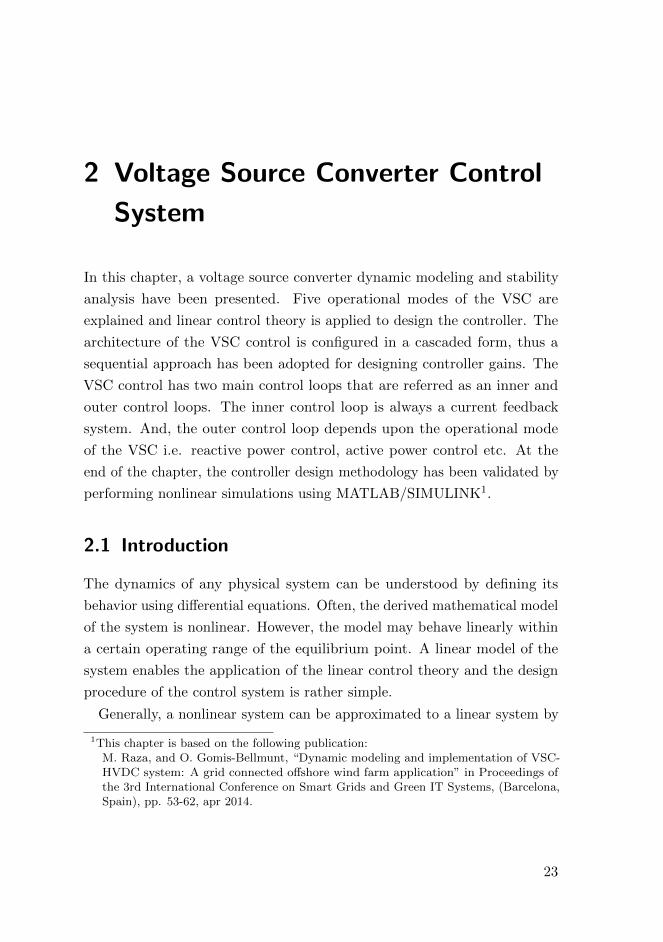
2 Voltage Source Converter Control

System

In this chapter, a voltage source converter dynamic modeling and stability

analysis have been presented. Five operational modes of the VSC are

explained and linear control theory is applied to design the controller. The

architecture of the VSC control is configured in a cascaded form, thus a

sequential approach has been adopted for designing controller gains. The

VSC control has two main control loops that are referred as an inner and

outer control loops. The inner control loop is always a current feedback

system. And, the outer control loop depends upon the operational mode

of the VSC i.e. reactive power control, active power control etc. At the

end of the chapter, the controller design methodology has been validated by

performing nonlinear simulations using MATLAB/SIMULINK1.

2.1 Introduction

The dynamics of any physical system can be understood by defining its

behavior using differential equations. Often, the derived mathematical model

of the system is nonlinear. However, the model may behave linearly within

a certain operating range of the equilibrium point. A linear model of the

system enables the application of the linear control theory and the design

procedure of the control system is rather simple.

Generally, a nonlinear system can be approximated to a linear system by

1This chapter is based on the following publication:M. Raza, and O. Gomis-Bellmunt, “Dynamic modeling and implementation of VSC-HVDC system: A grid connected offshore wind farm application” in Proceedings ofthe 3rd International Conference on Smart Grids and Green IT Systems, (Barcelona,Spain), pp. 53-62, apr 2014.

23

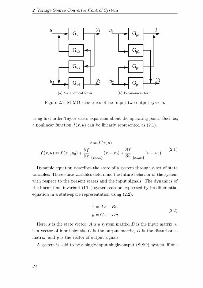
2 Voltage Source Converter Control System

Gv1

Gv2

Gv3

Gv4

u1 y1

u2 y2

(a) V-canonical form

Gp1

Gp2

Gp3

Gp4

u1 y1

u2y2

(b) P-canonical form

Figure 2.1: MIMO structures of two input two output system.

using first order Taylor series expansion about the operating point. Such as,

a nonlinear function f(x, u) can be linearly represented as (2.1).

x = f (x, u)

f (x, u) ≈ f (x0, u0) +∂f

∂x

∣∣∣∣x0,u0

(x− x0) +∂f

∂u

∣∣∣∣x0,u0

(u− u0)(2.1)

Dynamic equation describes the state of a system through a set of state

variables. These state variables determine the future behavior of the system

with respect to the present states and the input signals. The dynamics of

the linear time invariant (LTI) system can be expressed by its differential

equation in a state-space representation using (2.2).

x = Ax+Bu

y = Cx+Du(2.2)

Here, x is the state vector, A is a system matrix, B is the input matrix, u

is a vector of input signals, C is the output matrix, D is the disturbance

matrix, and y is the vector of output signals.

A system is said to be a single-input single-output (SISO) system, if one

24

2.1 Introduction

output is controlled by a single manipulated variable. However, most of

the systems do not exhibit such a simple control configuration. A system

may contain more than one output and being influenced by multiple input

signals. Such a control configuration is known as multi-input multi-output

(MIMO) system. In any MIMO system, there exist at least two or more

control loops and quit often these loops may act against each other in order

to achieve their respective objectives. Such an interaction between control

loops can cause the instability in the system. Several methods exist to

design control system for MIMO system such as singular value analysis,

pairing of controlled and manipulated variables, tuning of multi-loop PID

control systems, decoupling control strategies etc. A selection of a reliable

control technique depends on the structure of a linear system model in order

to ensure the control scheme resembles the dynamics of the system. The

two most common model representations of MIMO system are the V- and

P-canonical as illustrated in Figure 2.1. In the P-canonical form, the loop

interaction has the form of feed-forward coupling and in V-canonical form it

is feedback coupling. Contrary to P-canonical form, a change in one input

in V-canonical form will not only affect all outputs but it will also influence

the input signals. There is no explicit rule which model form is more useful.

However, any model form must represent the actual system dynamics and

should be able to give necessary data for the control system design.

In the dynamics of the power system components, the state variables

are voltage, current, power, and frequency. An instantaneous three phase

balanced voltage in an electrical network is a nonlinear time variant function

as expressed by (2.3). A time variant system explicitly depends on time and

is not stationary. A control system design is relatively complex for a time

variant system.

ua(t) = Um sin (ωt+ δ)

ub(t) = Um sin (ωt− 2π/3 + δ)

uc(t) = Um sin (ωt+ 2π/3 + δ)

(2.3)

Often, it is of interest for power system studies to analyze the change

in the network state variables with respect to the disturbances and the

25

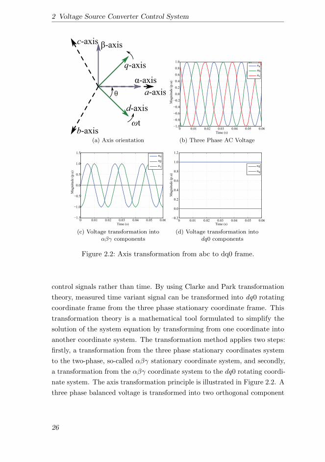
2 Voltage Source Converter Control System

a-axis

c-axis

b-axis

d-axis

q-axis

-axis

-axis

t

(a) Axis orientation

0 0.01 0.02 0.03 0.04 0.05 0.061.0

0.8

0.6

0.4

0.2

0.0

0.2

0.4

0.6

0.8

1.0ua

ub

uc

Time (s)

Mag

nit

ude

(p.u

)

(b) Three Phase AC Voltage

0 0.01 0.02 0.03 0.04 0.05 0.061.5

1.0

0.5

0.0

0.5

1.0

1.5u

u

u

Time (s)

Mag

nit

ude

(p.u

)

(c) Voltage transformation intoαβγ components

0 0.01 0.02 0.03 0.04 0.05 0.060.2

0.0

0.2

0.4

0.6

0.8

1.0

1.2

ud

uq

Time (s)

Mag

nit

ud

e (p

.u)

(d) Voltage transformation intodq0 components

Figure 2.2: Axis transformation from abc to dq0 frame.

control signals rather than time. By using Clarke and Park transformation

theory, measured time variant signal can be transformed into dq0 rotating

coordinate frame from the three phase stationary coordinate frame. This

transformation theory is a mathematical tool formulated to simplify the

solution of the system equation by transforming from one coordinate into

another coordinate system. The transformation method applies two steps:

firstly, a transformation from the three phase stationary coordinates system

to the two-phase, so-called αβγ stationary coordinate system, and secondly,

a transformation from the αβγ coordinate system to the dq0 rotating coordi-

nate system. The axis transformation principle is illustrated in Figure 2.2. A

three phase balanced voltage is transformed into two orthogonal component

26

2.1 Introduction

using (2.4). The α component is aligned with phase-a of the voltage signal.

The β component has a phase shift of −π/2 with respect to α, and the γ

component is always zero for a balanced system. Thus, voltage α and β

component can be expressed in complex form as (2.5).uα (t)

uβ (t)

uγ (t)

=2

3

1 −12 −1

2

0√

32 −

√3

212

12

12

ua (t)

ub (t)

uc (t)

(2.4)

uαβ = uα + juβ = Umej(δ(t)−π/2) ∵ δ(t) = ωt+ δ (2.5)

By rotating the coordinate frame with the angular frequency of the refe-

rence system, the two stationary orthogonal components can be transformed

into rotating components. Furthermore, if the rotating frame is aligned

with the measured busbar voltage, then the busbar is referred as reference

bus and the voltage d -component is Um, and the q-component is zero as

expressed by (2.6).

udq = ud + juq = uαβe−j(δ(t)−π/2) = Um + j0 (2.6)

Here, e−j(δ(t)−π/2) is the reference bus synchronization factor. Now, the

same approach is used to transform the measured current of a branch into

αβ components as expressed in (2.7).

iαβ = Imej(ψ(t)−π/2) ∵ ψ(t) = ωt+ ψ (2.7)

The current is then transformed into voltage synchronous rotating frame

by multiplying with the synchronization factor as given in (2.8). It is clear

that the current in the dq rotating frame is the function of current and load

angle.

idq = Imej(ψ(t)−π/2) · e−j(δ(t)−π/2)

= Ime−j(δ−ψ)

id + jiq = Im cos (δ − ψ)− j sin (δ − ψ)

(2.8)

The dq0 transformation matrix is orthogonal and it posses the property

27

2 Voltage Source Converter Control System

T (ωt) · T−1(ωt) = I. By applying inverse transformation, the signals can be

transformed from dq0 frame to abc frame i.e.

uabc(t) = T−1(δ(t))udq0ua (t)

ub (t)

uc (t)

=

sin (ωt) cos (ωt) 12

sin (ωt− 2π/3) cos (ωt− 2π/3) 12

sin (ωt+ 2π/3) cos (ωt+ 2π/3) 12

uduqu0

(2.9)

2.2 Voltage Source Converter Averaged Model

For the future offshore wind power plants development, it may be desired

for the application of HVDC system to have two main characteristics i.e

an ability to have bi-directional power flow (from AC to DC network, and

vice versa) without changing the voltage polarity, and the ability to create

an electrical grid. With the advancements in semiconductor devices such

as the insulated-gate bipolar transistor (IGBT), voltage source converters

(VSC) are gaining preference over line commutated converters (LCC). A

two-level converter is the simplest type of voltage source converter. As the

name implies, a two-level converter switches the output voltage between two

levels i.e +Udc/2 and −Udc/2, however it produces relatively more harmonics

compared to other types. Several pulse-width-modulation (PWM) techniques

are being developed to control the fundamental signal magnitude and to

reduce the harmonic in the output voltage. The most common modulation

strategies are selective harmonic elimination (SHE), sinusoidal pulse width

modulation (SPWM), and space vector modulation (SVM). In the PWM

technique, IGBTs are operated at a high frequency consequently converter

produces higher switching losses approx 2 to 3 %. Also, the step change in

the output voltage due to switching is large which limits the development of

high capacity converters.

In 2003, a new converter topology was developed, commonly known as

modular multilevel converter (MMC). The topology of a MMC-VSC is

illustrated in Figure 2.3. Each leg of the MMC is split into two arms

(upper and lower), and each arm consist of a series reactor and several

identical sub-modules connected in series. The sub-modules are individually

28

2.2 Voltage Source Converter Averaged Model

SM

SM

SM

SM

SM

SM

SM

SM

SM

SM

SM

SM

SM

SM

SM

SM

SM

SM

uaubuc

Udc

s1

s2Usm

ism

iaib

ic

SM

SM

SM

SM

SM

SM

Single Phase

SM

SM

SM

Lower Arm

Sub-Module

lau

lal

lbu lcu

lbl lcl

(a)

Idc

Pdc + Pac + Ploss = 0

Udcuabc(t)

iabc(t)

(b)

Figure 2.3: MMC VSC converter and an equivalent averaged model.

controllable and each have their own capacitive storage. There are different

sub-modules variants according to the semiconductor configuration, but the

most common one is a two level half bridge converter. In the two-level

half bridge variant, each sub-modules can produce two voltage levels i.e

Usm or zero. By connecting the sub-modules in series, the converter is able

to generate output voltage in high number of small discrete steps. The

converter output voltage can be generated very close to a sine-wave by

synthesizing the step voltages which can have very low harmonics content.

The use of voltage source converters has a large impact on the power

system and an appropriate model is required for the system analysis. The

detailed MMC-VSC model contains large number of switching devices which

slow down the simulation process due to the small simulation time steps. The

use of detailed models is restricted to component level and fault studies. An

averaged model which can reproduce the dynamic performance accurately is

sufficient for the study of slow dynamic stability phenomena and performance

analysis within a large scale AC network [93]. The averaged model of the

voltage source converter is given in Figure 2.3b. The ability of the VSC to

generate AC output voltage depends on the DC voltage level. Thus in the

29

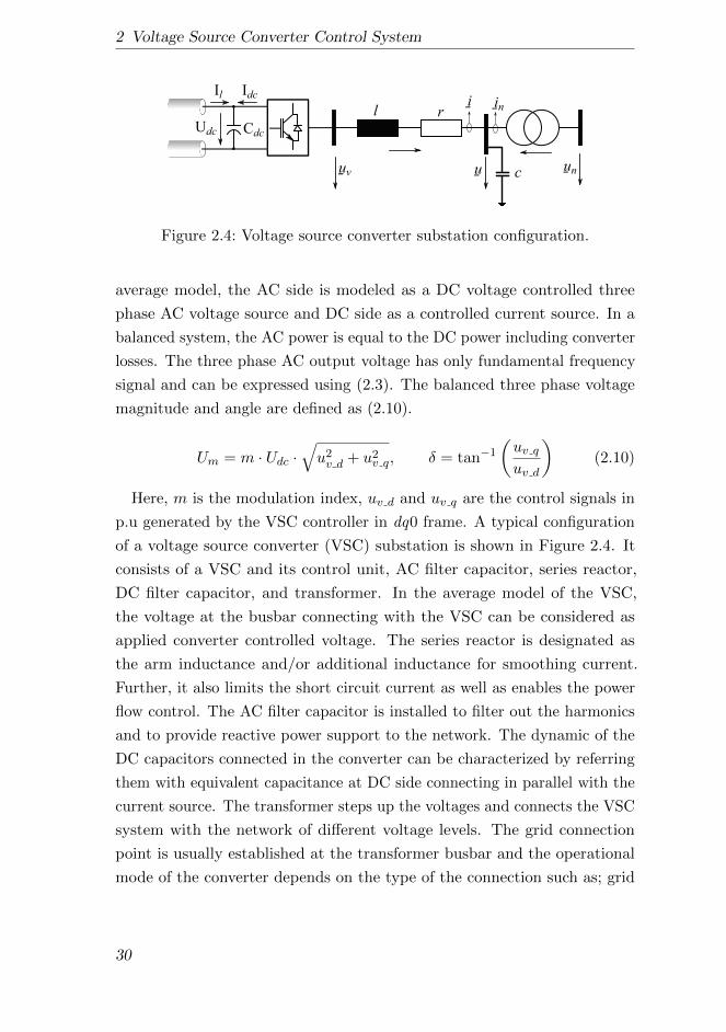
2 Voltage Source Converter Control System

i

Udc

l r

c

Cdc

Il Idcin

uv u un

Figure 2.4: Voltage source converter substation configuration.

average model, the AC side is modeled as a DC voltage controlled three

phase AC voltage source and DC side as a controlled current source. In a

balanced system, the AC power is equal to the DC power including converter

losses. The three phase AC output voltage has only fundamental frequency

signal and can be expressed using (2.3). The balanced three phase voltage

magnitude and angle are defined as (2.10).

Um = m · Udc ·√u2v d + u2

v q, δ = tan−1

(uv quv d

)(2.10)

Here, m is the modulation index, uv d and uv q are the control signals in

p.u generated by the VSC controller in dq0 frame. A typical configuration

of a voltage source converter (VSC) substation is shown in Figure 2.4. It

consists of a VSC and its control unit, AC filter capacitor, series reactor,

DC filter capacitor, and transformer. In the average model of the VSC,

the voltage at the busbar connecting with the VSC can be considered as

applied converter controlled voltage. The series reactor is designated as

the arm inductance and/or additional inductance for smoothing current.

Further, it also limits the short circuit current as well as enables the power

flow control. The AC filter capacitor is installed to filter out the harmonics

and to provide reactive power support to the network. The dynamic of the

DC capacitors connected in the converter can be characterized by referring

them with equivalent capacitance at DC side connecting in parallel with the

current source. The transformer steps up the voltages and connects the VSC

system with the network of different voltage levels. The grid connection

point is usually established at the transformer busbar and the operational

mode of the converter depends on the type of the connection such as; grid

30

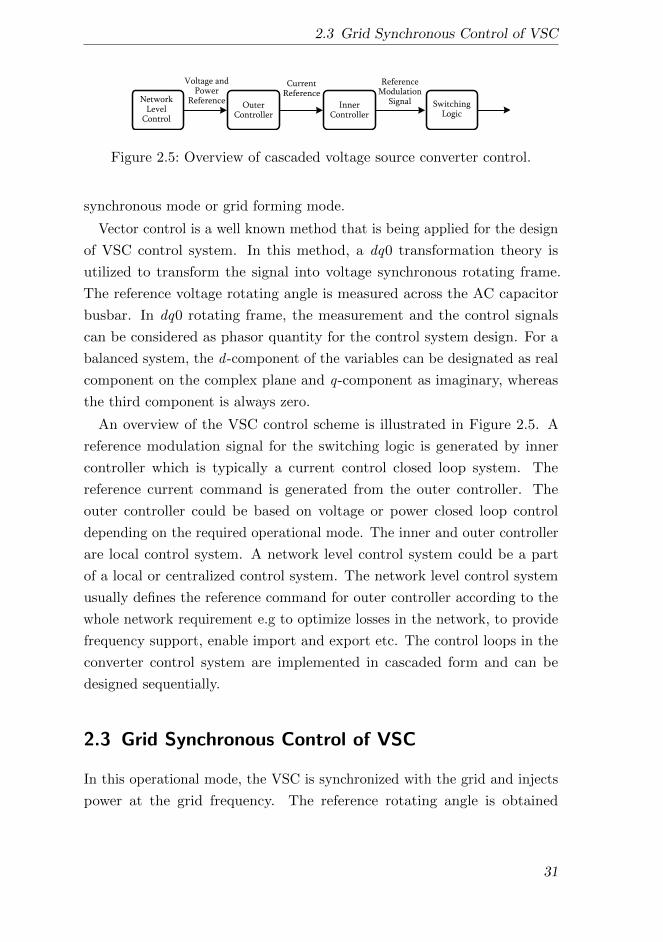
2.3 Grid Synchronous Control of VSC

InnerController

OuterController

NetworkLevel

Control

CurrentReference

ReferenceModulation

Signal

Voltage andPower

Reference SwitchingLogic

Figure 2.5: Overview of cascaded voltage source converter control.

synchronous mode or grid forming mode.

Vector control is a well known method that is being applied for the design

of VSC control system. In this method, a dq0 transformation theory is

utilized to transform the signal into voltage synchronous rotating frame.

The reference voltage rotating angle is measured across the AC capacitor

busbar. In dq0 rotating frame, the measurement and the control signals

can be considered as phasor quantity for the control system design. For a

balanced system, the d -component of the variables can be designated as real

component on the complex plane and q-component as imaginary, whereas

the third component is always zero.

An overview of the VSC control scheme is illustrated in Figure 2.5. A

reference modulation signal for the switching logic is generated by inner

controller which is typically a current control closed loop system. The

reference current command is generated from the outer controller. The

outer controller could be based on voltage or power closed loop control

depending on the required operational mode. The inner and outer controller

are local control system. A network level control system could be a part

of a local or centralized control system. The network level control system

usually defines the reference command for outer controller according to the

whole network requirement e.g to optimize losses in the network, to provide

frequency support, enable import and export etc. The control loops in the

converter control system are implemented in cascaded form and can be

designed sequentially.

2.3 Grid Synchronous Control of VSC

In this operational mode, the VSC is synchronized with the grid and injects

power at the grid frequency. The reference rotating angle is obtained

31

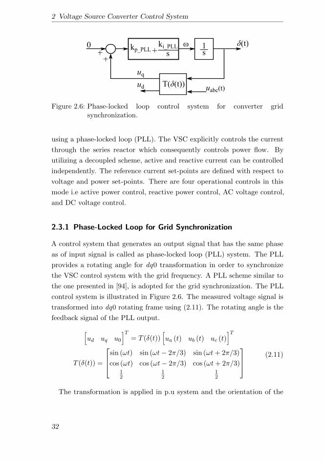
2 Voltage Source Converter Control System

1s

kp_PLLki_PLLs

(t)

T( (t))uabc(t)

0

ud

uq

Figure 2.6: Phase-locked loop control system for converter gridsynchronization.

using a phase-locked loop (PLL). The VSC explicitly controls the current

through the series reactor which consequently controls power flow. By

utilizing a decoupled scheme, active and reactive current can be controlled

independently. The reference current set-points are defined with respect to

voltage and power set-points. There are four operational controls in this

mode i.e active power control, reactive power control, AC voltage control,

and DC voltage control.

2.3.1 Phase-Locked Loop for Grid Synchronization

A control system that generates an output signal that has the same phase

as of input signal is called as phase-locked loop (PLL) system. The PLL

provides a rotating angle for dq0 transformation in order to synchronize

the VSC control system with the grid frequency. A PLL scheme similar to

the one presented in [94], is adopted for the grid synchronization. The PLL

control system is illustrated in Figure 2.6. The measured voltage signal is

transformed into dq0 rotating frame using (2.11). The rotating angle is the

feedback signal of the PLL output.[ud uq u0

]T= T (δ(t))

[ua (t) ub (t) uc (t)

]TT (δ(t)) =

sin (ωt) sin (ωt− 2π/3) sin (ωt+ 2π/3)

cos (ωt) cos (ωt− 2π/3) cos (ωt+ 2π/3)12

12

12

(2.11)

The transformation is applied in p.u system and the orientation of the

32

2.3 Grid Synchronous Control of VSC

dq frame is aligned such that at synchronization the d -component would be

1.0 p.u, and the q-component is zero. The proportional-plus-integral (PI)

control scheme is applied to acquire the desired performance and to ensure

system stability. By applying Laplace transformation, the PLL closed loop

control can be represented with the second order transfer function and the

selection of the controller gains can be made using (2.12).

G(s) =kp PLL · s+ ki PLL

s2 + kp PLL · s+ ki PLL

kp PLL = 2ωnζ, ki PLL =1

ω2n

(2.12)

Here, kp PLL, and ki PLL are the proportional and integral gains, ωn is the

natural frequency, and ζ is the damping factor. Further detail is given in [94].

This type of PLL is the simplest and widely applied in different power system

applications. It is also known as ‘Synchronous Frame PLL (SF-PLL)’. There

are other advanced methods of phase detection such as PQ-PLL based on

instantaneous real and imaginary power theory, double synchronous frame

PLL (DSF-PLL), sinusoidal signal integrator PLL (SSI-PLL), double second

order generalized integrator PLL (DSOGI-PLL), three phase magnitude PLL

(3M-PLL), enhanced PLL (EPLL), etc. The SF-PLL with high bandwidth

provides fast and precise phase detection of the non distorted input signal.

The SF-PLL can still exhibit sufficient performance with the input signal

having high order harmonics on the cost of PLL response speed. Furthermore,

SF-PLL scheme cannot be applied straightforward to single phase system and

it provides the average information of phase, frequency, and magnitude rather

than individual phases. In [95], it is highlighted that the SF-PLL may fail to

synchronize in some adverse conditions during start-up. It may achieved the

stable operational point in the presence of harmonics synchronized with the

subharmonic frequency. The PQ-PLL usually provides remedy to this issue.

Another scheme such as DSF-PLL, also cover the limitation of SF-PLL

by detecting the phase angle using both positive and negative sequence

components of the input signal. There are many more PLL schemes however

the selection of the suitable scheme depends on the specific requirements

and applications [96].

33

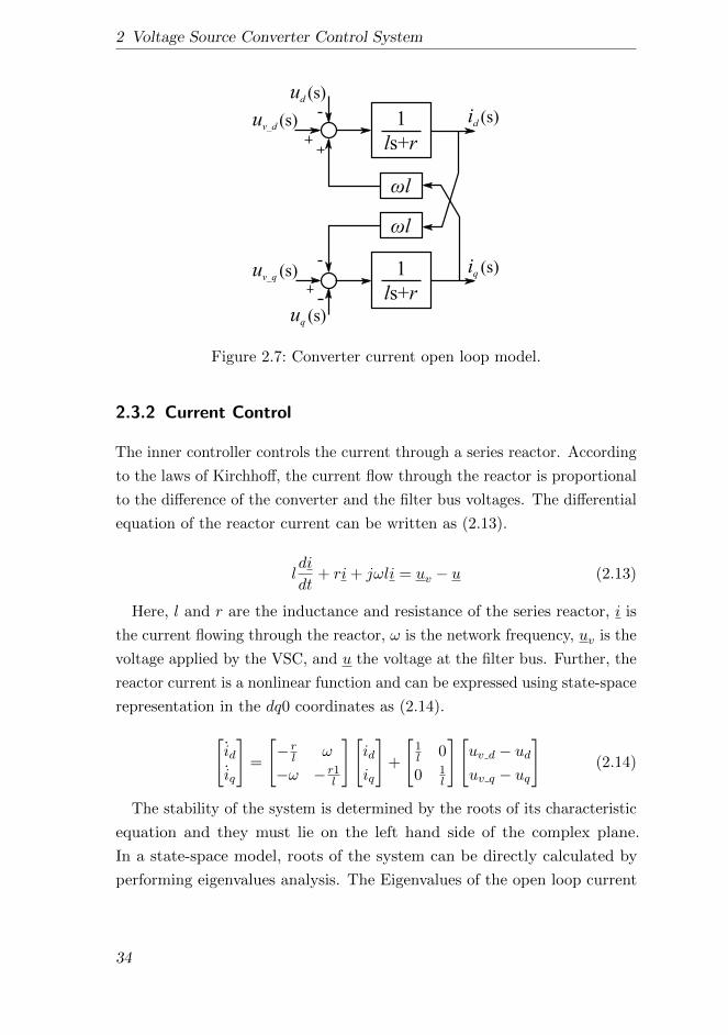
2 Voltage Source Converter Control System

1

ls+r

1

ls+r

l

l

id (s)

iq (s)

ud (s)

uq (s)

uv_d (s)

uv_q (s)

Figure 2.7: Converter current open loop model.

2.3.2 Current Control

The inner controller controls the current through a series reactor. According

to the laws of Kirchhoff, the current flow through the reactor is proportional

to the difference of the converter and the filter bus voltages. The differential

equation of the reactor current can be written as (2.13).

ldi

dt+ ri+ jωli = uv − u (2.13)

Here, l and r are the inductance and resistance of the series reactor, i is

the current flowing through the reactor, ω is the network frequency, uv is the

voltage applied by the VSC, and u the voltage at the filter bus. Further, the

reactor current is a nonlinear function and can be expressed using state-space

representation in the dq0 coordinates as (2.14).[id

iq

]=

[− rl ω

−ω − r1l

][id

iq

]+

[1l 0

0 1l

][uv d − uduv q − uq

](2.14)

The stability of the system is determined by the roots of its characteristic

equation and they must lie on the left hand side of the complex plane.

In a state-space model, roots of the system can be directly calculated by

performing eigenvalues analysis. The Eigenvalues of the open loop current

34

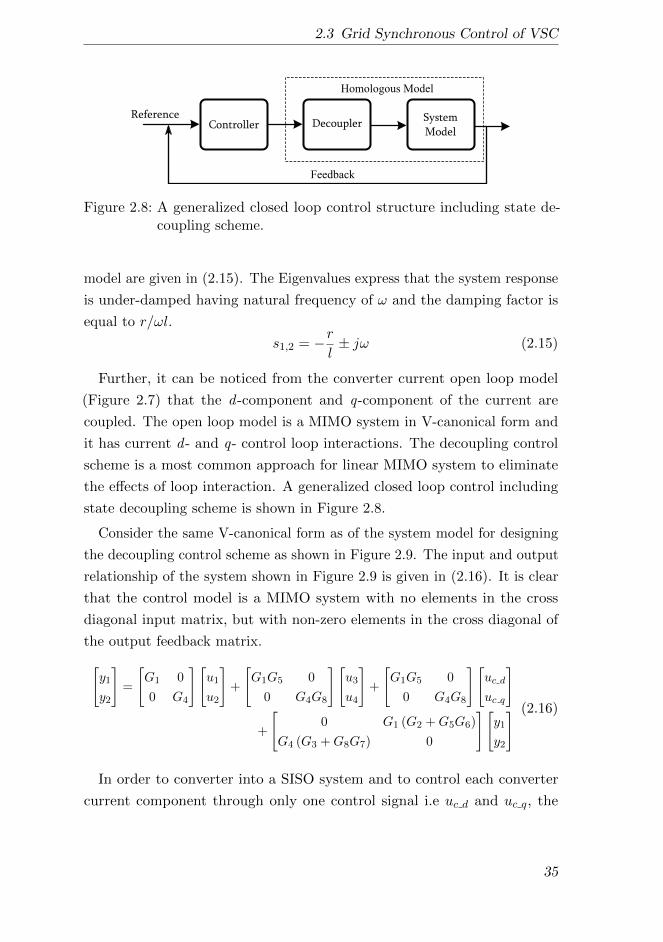
2.3 Grid Synchronous Control of VSC

DecouplerControllerReference System

Model

Homologous Model

Feedback

Figure 2.8: A generalized closed loop control structure including state de-coupling scheme.

model are given in (2.15). The Eigenvalues express that the system response

is under-damped having natural frequency of ω and the damping factor is

equal to r/ωl.

s1,2 = −rl± jω (2.15)

Further, it can be noticed from the converter current open loop model

(Figure 2.7) that the d -component and q-component of the current are

coupled. The open loop model is a MIMO system in V-canonical form and

it has current d - and q- control loop interactions. The decoupling control

scheme is a most common approach for linear MIMO system to eliminate

the effects of loop interaction. A generalized closed loop control including

state decoupling scheme is shown in Figure 2.8.

Consider the same V-canonical form as of the system model for designing

the decoupling control scheme as shown in Figure 2.9. The input and output

relationship of the system shown in Figure 2.9 is given in (2.16). It is clear

that the control model is a MIMO system with no elements in the cross

diagonal input matrix, but with non-zero elements in the cross diagonal of

the output feedback matrix.[y1

y2

]=

[G1 0

0 G4

][u1

u2

]+

[G1G5 0

0 G4G8

][u3

u4

]+

[G1G5 0

0 G4G8

][uc d

uc q

]

+

[0 G1 (G2 +G5G6)

G4 (G3 +G8G7) 0

][y1

y2

] (2.16)

In order to converter into a SISO system and to control each converter

current component through only one control signal i.e uc d and uc q, the

35

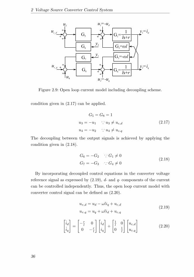
2 Voltage Source Converter Control System

1

ls+r

G2= l

y1=id

y2=iq

u1=-ud

u2=-uq

uc_d

uc_q

G1=

1

ls+rG4=

G3=- ly

1

y2

u3

u4

G5

G6

G7

G8

Figure 2.9: Open loop current model including decoupling scheme.

condition given in (2.17) can be applied.

G5 = G8 = 1

u3 = −u1 ∵ u3 6= uc d

u4 = −u2 ∵ u4 6= uc q

(2.17)

The decoupling between the output signals is achieved by applying the

condition given in (2.18).

G6 = −G2 ∵ G1 6= 0

G7 = −G3 ∵ G4 6= 0(2.18)

By incorporating decoupled control equations in the converter voltage

reference signal as expressed by (2.19), d- and q- components of the current

can be controlled independently. Thus, the open loop current model with

converter control signal can be defined as (2.20).

uv d = ud − ωliq + uc d

uv q = uq + ωlid + uc q(2.19)

[id

iq

]=

[− rl 0

0 − rl

][id

iq

]+

[1l 0

0 1l

][uc d

uc q

](2.20)

36

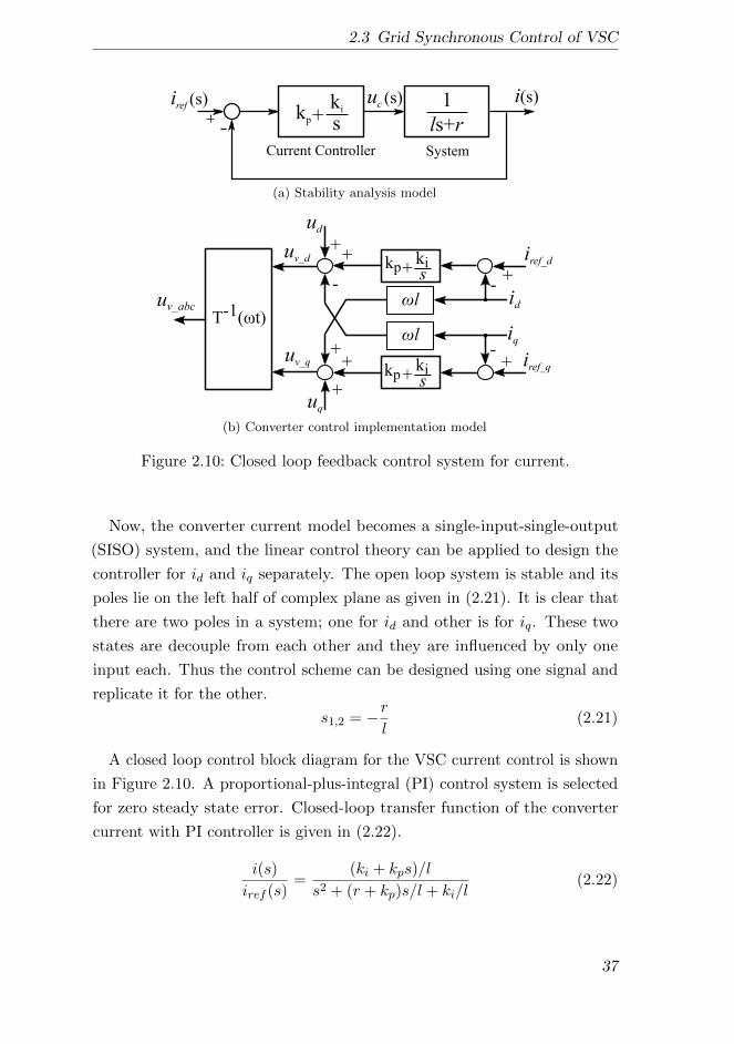
2.3 Grid Synchronous Control of VSC

i(s)uc (s)iref (s) 1

ls+rkp s

Current Controller System

ki+

(a) Stability analysis model

kp+kis

kp+kis

+

-+

+-

+

-

++

+

T-1( t)id

iq

ud

uq

l

l

iref_d

iref_q

uv_d

uv_q

uv_abc

(b) Converter control implementation model

Figure 2.10: Closed loop feedback control system for current.

Now, the converter current model becomes a single-input-single-output

(SISO) system, and the linear control theory can be applied to design the

controller for id and iq separately. The open loop system is stable and its

poles lie on the left half of complex plane as given in (2.21). It is clear that

there are two poles in a system; one for id and other is for iq. These two

states are decouple from each other and they are influenced by only one

input each. Thus the control scheme can be designed using one signal and

replicate it for the other.

s1,2 = −rl

(2.21)

A closed loop control block diagram for the VSC current control is shown

in Figure 2.10. A proportional-plus-integral (PI) control system is selected

for zero steady state error. Closed-loop transfer function of the converter

current with PI controller is given in (2.22).

i(s)

iref (s)=

(ki + kps)/l

s2 + (r + kp)s/l + ki/l(2.22)

37

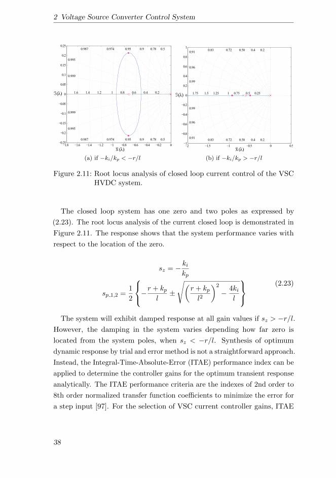
2 Voltage Source Converter Control System

1.8 1.6 1.4 1.2 1 0.8 0.6 0.4 0.2 00.25

0.2

0.15

0.1

0.05

0

0.05

0.1

0.15

0.2

0.250.50.780.90.950.9740.987

0.995

0.999

0.50.780.90.950.9740.987

0.995

0.999

0.20.40.60.811.21.41.6

( )

( )

(a) if −ki/kp < −r/l

2 1.5 1 0.5 0 0.51

0.8

0.6

0.4

0.2

0

0.2

0.4

0.6

0.8

10.20.40.580.720.83

0.91

0.96

0.99

0.20.40.580.720.830.91

0.96

0.99

0.250.50.7511.251.51.75

( )

( )

(b) if −ki/kp > −r/l

Figure 2.11: Root locus analysis of closed loop current control of the VSCHVDC system.

The closed loop system has one zero and two poles as expressed by

(2.23). The root locus analysis of the current closed loop is demonstrated in

Figure 2.11. The response shows that the system performance varies with

respect to the location of the zero.

sz = − kikp

sp 1,2 =1

2

−r + kpl±

√(r + kpl2

)2

− 4kil

(2.23)

The system will exhibit damped response at all gain values if sz > −r/l.However, the damping in the system varies depending how far zero is

located from the system poles, when sz < −r/l. Synthesis of optimum

dynamic response by trial and error method is not a straightforward approach.

Instead, the Integral-Time-Absolute-Error (ITAE) performance index can be

applied to determine the controller gains for the optimum transient response

analytically. The ITAE performance criteria are the indexes of 2nd order to

8th order normalized transfer function coefficients to minimize the error for

a step input [97]. For the selection of VSC current controller gains, ITAE

38

2.3 Grid Synchronous Control of VSC

600 500 400 300 200 100 0250

200

150

100

50

0

50

100

150

200

2500.20.40.560.70.810.9

0.955

0.988

0.20.40.560.70.810.9

0.955

0.988

100200300400500

( )

( )

(a) ξ = 0.7, wn = 286 rad/s

Time (s)

i(t)

0 0.005 0.01 0.015 0.02 0.0250

0.2

0.4

0.6

0.8

1

1.2

1.4

(b) Step response: Ts = 20 ms

Figure 2.12: Under-damped performance analysis of the closed loop currentcontrol.

criteria is applied by using (2.24) for zero-displacement error.

s2 + 1.4ωns+ ω2n = s2 + (r + kp)s/l + ki/l

kp = 1.4ωnl − r, ki = ω2nl

Ts =4

0.7ωn∵ ξ = 0.7

(2.24)

Here, Ts is the settling time, and ωn is the natural frequency of the closed

loop. It is to be noticed that the standard ITAE criteria is provided for the

transfer function without finite zeros. This criteria can also be applied up to

ξ < 0.8 for the transfer function that has one zero. The current closed loop

performance is shown in Figure 2.12 for the under-damped condition. The

overshoot in the current response can be observed in this condition. The

damping in the response is increased when zeros move toward the poles. The

zeros of the closed loop system influence the transient response significantly

when they are located near to the dominant poles.

The influence of the zero on the current closed loop system can be analyzed

by placing the zero at the dominate pole as expressed in (2.25). By substi-

tuting the value of ki in (2.23), the current closed loop transfer function can

be derived from the zeros and poles of the system as given by (2.26).

39

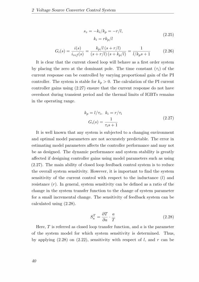
2 Voltage Source Converter Control System

sz = −ki/kp = −r/l,

ki = rkp/l(2.25)

Gi(s) =i(s)

iref (s)=

kp/l (s+ r/l)

(s+ r/l) (s+ kp/l)=

1

l/kps+ 1(2.26)

It is clear that the current closed loop will behave as a first order system

by placing the zero at the dominant pole. The time constant (τi) of the

current response can be controlled by varying proportional gain of the PI

controller. The system is stable for kp > 0. The calculation of the PI current

controller gains using (2.27) ensure that the current response do not have

overshoot during transient period and the thermal limits of IGBTs remains

in the operating range.

kp = l/τi, ki = r/τi

Gi(s) =1

τis+ 1

(2.27)

It is well known that any system is subjected to a changing environment

and optimal model parameters are not accurately predictable. The error in

estimating model parameters affects the controller performance and may not

be as designed. The dynamic performance and system stability is greatly

affected if designing controller gains using model parameters such as using

(2.27). The main ability of closed loop feedback control system is to reduce

the overall system sensitivity. However, it is important to find the system

sensitivity of the current control with respect to the inductance (l) and

resistance (r). In general, system sensitivity can be defined as a ratio of the

change in the system transfer function to the change of system parameter

for a small incremental change. The sensitivity of feedback system can be

calculated using (2.28).

STa =∂T

∂a· aT

(2.28)

Here, T is referred as closed loop transfer function, and a is the parameter

of the system model for which system sensitivity is determined. Thus,

by applying (2.28) on (2.22), sensitivity with respect of l, and r can be

40

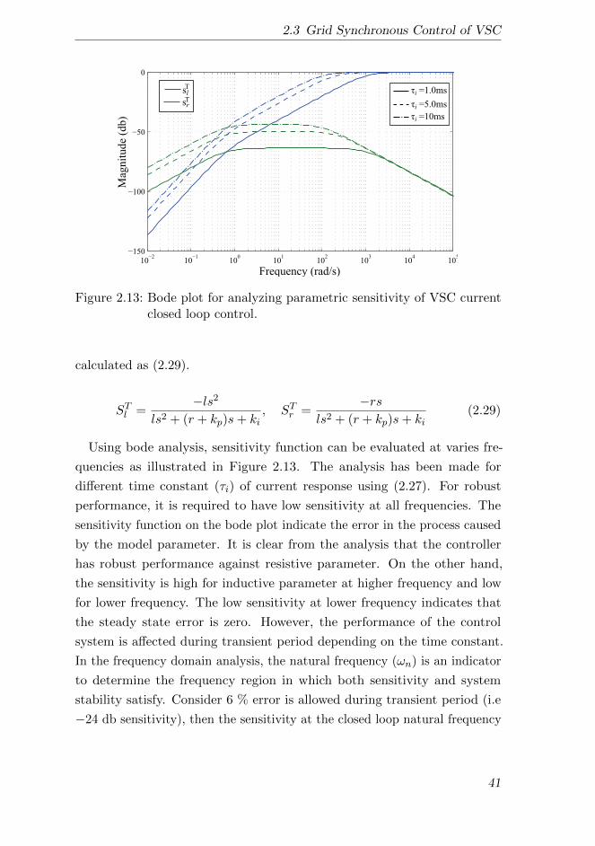
2.3 Grid Synchronous Control of VSC

102

101

100

101

102

103

104

105

150

100

50

0

Frequency (rad/s)

Mag

nit

ud

e (d

b)

srT

slT

i =1.0ms

i =5.0ms

i =10ms

Figure 2.13: Bode plot for analyzing parametric sensitivity of VSC currentclosed loop control.

calculated as (2.29).

STl =−ls2

ls2 + (r + kp)s+ ki, STr =

−rsls2 + (r + kp)s+ ki

(2.29)

Using bode analysis, sensitivity function can be evaluated at varies fre-

quencies as illustrated in Figure 2.13. The analysis has been made for

different time constant (τi) of current response using (2.27). For robust

performance, it is required to have low sensitivity at all frequencies. The

sensitivity function on the bode plot indicate the error in the process caused

by the model parameter. It is clear from the analysis that the controller

has robust performance against resistive parameter. On the other hand,

the sensitivity is high for inductive parameter at higher frequency and low

for lower frequency. The low sensitivity at lower frequency indicates that

the steady state error is zero. However, the performance of the control

system is affected during transient period depending on the time constant.

In the frequency domain analysis, the natural frequency (ωn) is an indicator

to determine the frequency region in which both sensitivity and system

stability satisfy. Consider 6 % error is allowed during transient period (i.e

−24 db sensitivity), then the sensitivity at the closed loop natural frequency

41

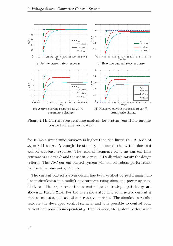
2 Voltage Source Converter Control System

0.98 0.99 1 1.01 1.02 1.03 1.04 1.05 1.06 1.07 1.08 1.09 1.10

0.2

0.4

0.6

0.8

1

Time (s)

i d (

p.u

)

iref

=1.0 ms

=5.0 ms

=10 ms

i

i

i

(a) Active current step response

1.48 1.49 1.5 1.51 1.52 1.53 1.54 1.55 1.56 1.57 1.58 1.59 1.60

0.1

0.2

0.3

0.4

0.5

i q (

p.u

)

iref

=1.0 ms

=5.0 ms

=10 ms

i

i

i

Time (s)

(b) Reactive current step response

0.98 0.99 1 1.01 1.02 1.03 1.04 1.05 1.06 1.07 1.08 1.09 1.10

0.2

0.4

0.6

0.8

1

iref

=1.0 ms

=5.0 ms

=10 ms

i

i

i

Time (s)

(c) Active current response at 20 %parametric change

1.48 1.49 1.5 1.51 1.52 1.53 1.54 1.55 1.56 1.57 1.58 1.59 1.60

0.1

0.2

0.3

0.4

0.5

iref

=1.0 ms

=5.0 ms

=10 ms

i

i

i

Time (s)

(d) Reactive current response at 20 %parametric change

Figure 2.14: Current step response analysis for system sensitivity and de-coupled scheme verification.

for 10 ms current time constant is higher than the limits i.e −21.6 db at

ωn = 8.41 rad/s. Although the stability is ensured, the system does not

exhibit a robust response. The natural frequency for 5 ms current time

constant is 11.5 rad/s and the sensitivity is −24.8 db which satisfy the design

criteria. The VSC current control system will exhibit robust performance

for the time constant τi ≤ 5 ms.

The current control system design has been verified by performing non-

linear simulation in simulink environment using simscape power systems

block set. The responses of the current subjected to step input change are

shown in Figure 2.14. For the analysis, a step change in active current is

applied at 1.0 s, and at 1.5 s in reactive current. The simulation results

validate the developed control scheme, and it is possible to control both

current components independently. Furthermore, the system performance

42

2.3 Grid Synchronous Control of VSC

1

ltrs+rtr

1

ltrs+rtr

1

is+1

ltr

ltr

c

c

1

c

1

c

1

is+1

iref_d

iref_q

id

iq

in_d

in_q

ud

uq

un_q

un_d

Figure 2.15: Grid connected VSC open loop control block diagram withrespect to the outer controller.

is more robust for less than 5 ms current time constant. The parametric

sensitivity is analyzed by changing the series reactor value by 20 %. It is

clear that the current transient response for time constant greater than 5 ms

is significantly influenced, and the steady state reaches very late. At slower

current controller, the transient decoupling between the current component

may also not be achieved properly.

2.3.3 Power-Voltage Control

The operational principle of the VSC in grid synchronous mode is defined

by the outer control mode which depends on the feedback signal employed

in the outer controller. The outer controller regulates the current reference

signal according to the measured voltage or power signal. The dynamics

of the outer controller depends on the network elements that are being

involved in the feedback signal. Typically, a VSC substation is connected

with the network at the transformer bus, but the outer controller perform

the voltage control either at the filter bus or the power control through the

series reactor. In this regard, the open loop dynamic model can be developed

for outer controller performance analysis by defining filter bus voltage and

43

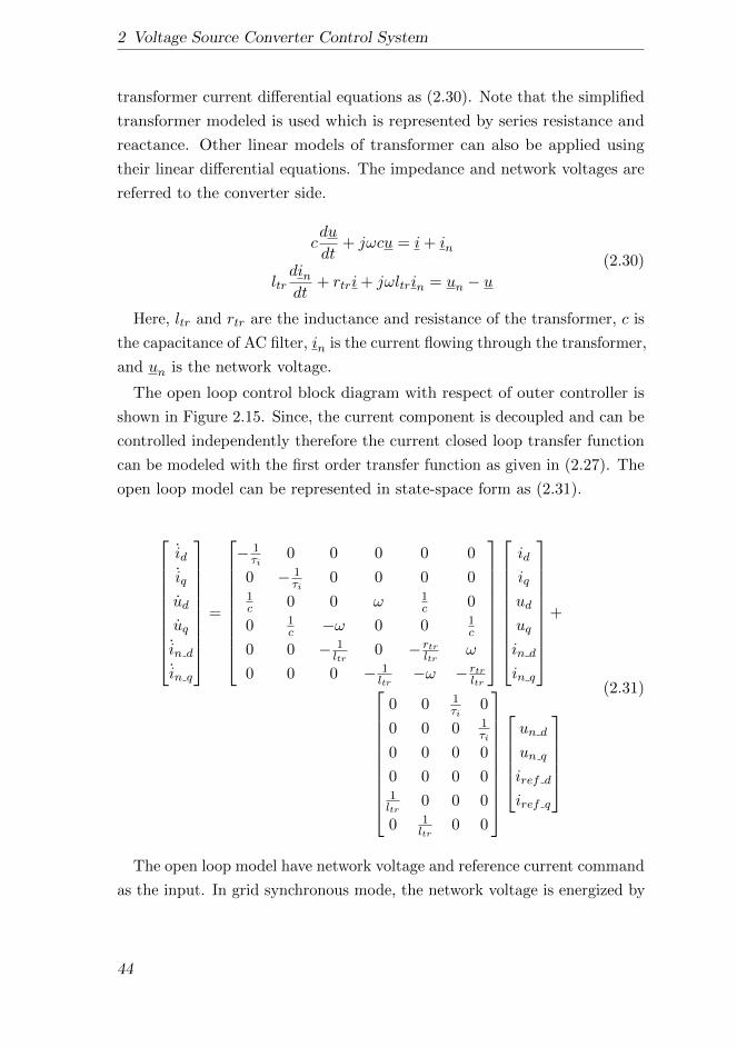
2 Voltage Source Converter Control System

transformer current differential equations as (2.30). Note that the simplified

transformer modeled is used which is represented by series resistance and

reactance. Other linear models of transformer can also be applied using

their linear differential equations. The impedance and network voltages are

referred to the converter side.

cdu

dt+ jωcu = i+ in

ltrdindt

+ rtri+ jωltrin = un − u(2.30)

Here, ltr and rtr are the inductance and resistance of the transformer, c is

the capacitance of AC filter, in is the current flowing through the transformer,

and un is the network voltage.

The open loop control block diagram with respect of outer controller is

shown in Figure 2.15. Since, the current component is decoupled and can be

controlled independently therefore the current closed loop transfer function

can be modeled with the first order transfer function as given in (2.27). The

open loop model can be represented in state-space form as (2.31).

id

iq

ud

uq

in d

in q

=

− 1τi

0 0 0 0 0

0 − 1τi

0 0 0 01c 0 0 ω 1

c 0

0 1c −ω 0 0 1

c

0 0 − 1ltr

0 − rtrltr

ω

0 0 0 − 1ltr

−ω − rtrltr

id

iq

ud

uq

in d

in q

+

0 0 1τi

0

0 0 0 1τi

0 0 0 0

0 0 0 01ltr

0 0 0

0 1ltr

0 0

un d

un q

iref d

iref q

(2.31)

The open loop model have network voltage and reference current command

as the input. In grid synchronous mode, the network voltage is energized by

44

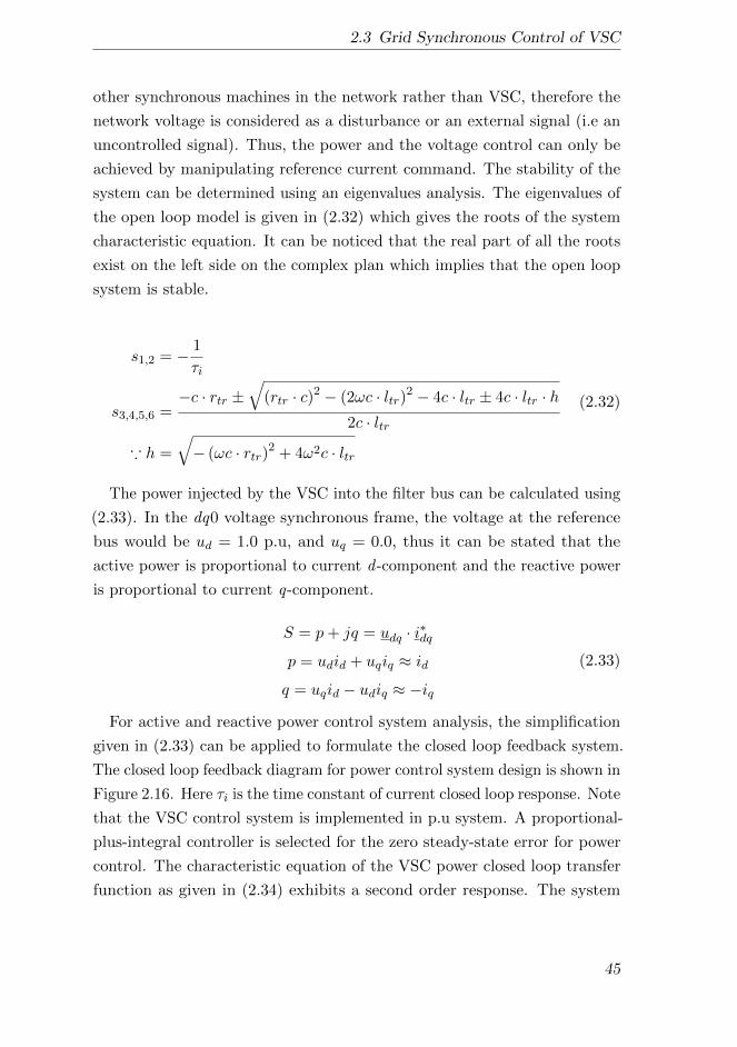
2.3 Grid Synchronous Control of VSC

other synchronous machines in the network rather than VSC, therefore the

network voltage is considered as a disturbance or an external signal (i.e an

uncontrolled signal). Thus, the power and the voltage control can only be

achieved by manipulating reference current command. The stability of the

system can be determined using an eigenvalues analysis. The eigenvalues of

the open loop model is given in (2.32) which gives the roots of the system

characteristic equation. It can be noticed that the real part of all the roots

exist on the left side on the complex plan which implies that the open loop

system is stable.

s1,2 = − 1

τi

s3,4,5,6 =−c · rtr ±

√(rtr · c)2 − (2ωc · ltr)2 − 4c · ltr ± 4c · ltr · h

2c · ltr

∵ h =

√− (ωc · rtr)2 + 4ω2c · ltr

(2.32)

The power injected by the VSC into the filter bus can be calculated using

(2.33). In the dq0 voltage synchronous frame, the voltage at the reference

bus would be ud = 1.0 p.u, and uq = 0.0, thus it can be stated that the

active power is proportional to current d -component and the reactive power

is proportional to current q-component.

S = p+ jq = udq · i∗dqp = udid + uqiq ≈ idq = uqid − udiq ≈ −iq

(2.33)

For active and reactive power control system analysis, the simplification

given in (2.33) can be applied to formulate the closed loop feedback system.

The closed loop feedback diagram for power control system design is shown in

Figure 2.16. Here τi is the time constant of current closed loop response. Note

that the VSC control system is implemented in p.u system. A proportional-

plus-integral controller is selected for the zero steady-state error for power

control. The characteristic equation of the VSC power closed loop transfer

function as given in (2.34) exhibits a second order response. The system

45

2 Voltage Source Converter Control System

1

is+1kois

kop+y(s)u(s)

iref (s)

(a) Power model for stability analysis

iref_dpset

p

kois

kop+

(b) Active power control implementation

iref_qqset koi

skop+

q(c) Reactive power control

implementation

Figure 2.16: Closed loop feedback diagram for power controller design ingrid synchronous mode.

response varies from over-damped to under-damped response according to

the location of zeros. The frequency and dynamic response of power control

for over-damped system is shown in Figure 2.17.

y(s)

u(s)=

kop (s+ koi/kop)

τis2 + (kop + 1) s+ koi

1/τi > koi/kop, kop > 0

(2.34)

Yet again, it is desirable to not to have overshoot during transient period

in the power to avoid stress on the IGBT. Therefore, the zero of the closed

loop transfer function must be placed according to the condition given in

(2.34). A nonlinear step analysis for over-damped system response is shown

in Figure 2.17c. For the analysis, a step change in active and reactive power

is applied at 1.0 s, and 1.5 s respectively. It can be seen that active and

reactive power are controlled individually and they are decoupled from each

other. Moreover, the bandwidth of power closed loop response is less than

the current response. The rise time of 100 ms is considered as a design

condition. Faster rise time may introduce transient coupling between active

and reactive power due to weak grid voltage.

Typically, active power control mode is set for performing import and

46

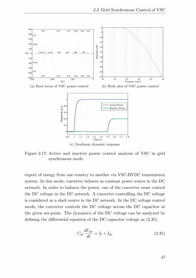
2.3 Grid Synchronous Control of VSC

1500 1000 500 0500

400

300

200

100

0

100

200

300

400

5000.240.480.660.780.870.93

0.97

0.992

0.240.480.660.780.870.93

0.97

0.992

2004006008001e+031.2e+03

( )

( )

(a) Root locus of VSC power control

100

101

102

103

104

105

50

45

40

35

30

25

20

15

10

5

0

Frequency (rad/s)

Mag

nit

ude

(dB

)

(b) Bode plot of VSC power control

0.9 1 1.1 1.2 1.3 1.4 1.5 1.6 1.7 1.8

0

0.2

0.4

0.6

0.8

1

Time (s)

Mag

nit

ud

e (p

.u) Active Power

Reactive Power

(c) Nonlinear dynamic response

Figure 2.17: Active and reactive power control analysis of VSC in gridsynchronous mode.

export of energy from one country to another via VSC-HVDC transmission

system. In this mode, converter behaves as constant power source in the DC

network. In order to balance the power, one of the converter must control

the DC voltage in the DC network. A converter controlling the DC voltage

is considered as a slack source in the DC network. In the DC voltage control

mode, the converter controls the DC voltage across the DC capacitor at

the given set-point. The dynamics of the DC voltage can be analyzed by

defining the differential equation of the DC capacitor voltage as (2.35).

CdcdUdcdt

= Il + Idc (2.35)

47

2 Voltage Source Converter Control System

1

is+1koi_dc

skop_dc +

Udc_ref (s) 1Cdcs

is+1is

Udc(s)

Il(s)

(a) Stability model of DC voltage control

koi_dc

skop_dc +

Udc_ref

Udc Il

iref_d

(b) DC voltage control implementation

Figure 2.18: Closed loop block diagram of VSC DC voltage control.

Here, Udc is the voltage across DC capacitor, Cdc is the DC capacitor

value, Il is the current injected by the DC network, and Idc is the DC current

of the VSC. In the lossless converter, AC active power is equal to DC active

power thus DC current can be approximated to d -axis of the AC current as

expressed by (2.36).

pac = pdc ⇒ udid = UdcIdc

id ≈ Idc(2.36)

The DC voltage control closed loop stability model and its implementation

for nonlinear simulation is illustrated in Figure 2.18. Note that in the

nonlinear control implementation Idc = −id to maintain the sign convention.

A proportional-plus-integral control scheme is applied for zero steady state

error. The dynamics of the DC voltage is the function of two inputs i.e the

network DC current and reference DC voltage set-point. The closed loop

transfer functions with respect of both inputs are given in (2.37).

Tu(s) =Udc(s)

Udc ref (s)=

kop dcs+ koi dcτiCdcs3 + Cdcs2 + kop dcs+ koi dc

Ti(s) =Udc(s)

Il(s)=

τis2

τiCdcs3 + Cdcs2 + kop dcs+ koi dc

(2.37)

48

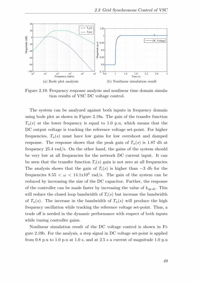
2.3 Grid Synchronous Control of VSC

100

101

102

103

104

105

100

80

60

40

20

0

20

40M

agnit

ude

(dB

)

Frequency (rad/s)

Tu(s)

Ti(s)

(a) Bode plot analysis

0.6 1 1.4 1.8 2.2 2.6 30.75

0.8

0.85

0.9

0.95

1

1.05

Time (s)

Mag

nit

ud

e (p

.u) DC Voltage

(b) Nonlinear simulation result

Figure 2.19: Frequency response analysis and nonlinear time domain simula-tion results of VSC DC voltage control.

The system can be analyzed against both inputs in frequency domain

using bode plot as shown in Figure 2.19a. The gain of the transfer function

Tu(s) at the lower frequency is equal to 1.0 p.u, which means that the

DC output voltage is tracking the reference voltage set-point. For higher

frequencies, Tu(s) must have low gains for low overshoot and damped

response. The response shows that the peak gain of Tu(s) is 1.87 db at

frequency 25.4 rad/s. On the other hand, the gains of the system should

be very low at all frequencies for the network DC current input. It can

be seen that the transfer function Ti(s) gain is not zero at all frequencies.

The analysis shows that the gain of Ti(s) is higher than −3 db for the

frequencies 8.55 < ω < 14.1x103 rad/s. The gain of the system can be

reduced by increasing the size of the DC capacitor. Further, the response

of the controller can be made faster by increasing the value of kop dc. This

will reduce the closed loop bandwidth of Ti(s) but increase the bandwidth

of Tu(s). The increase in the bandwidth of Tu(s) will produce the high

frequency oscillation while tracking the reference voltage set-point. Thus, a

trade off is needed in the dynamic performance with respect of both inputs

while tuning controller gains.

Nonlinear simulation result of the DC voltage control is shown in Fi-

gure 2.19b. For the analysis, a step signal in DC voltage set-point is applied

from 0.8 p.u to 1.0 p.u at 1.0 s, and at 2.5 s a current of magnitude 1.0 p.u

49

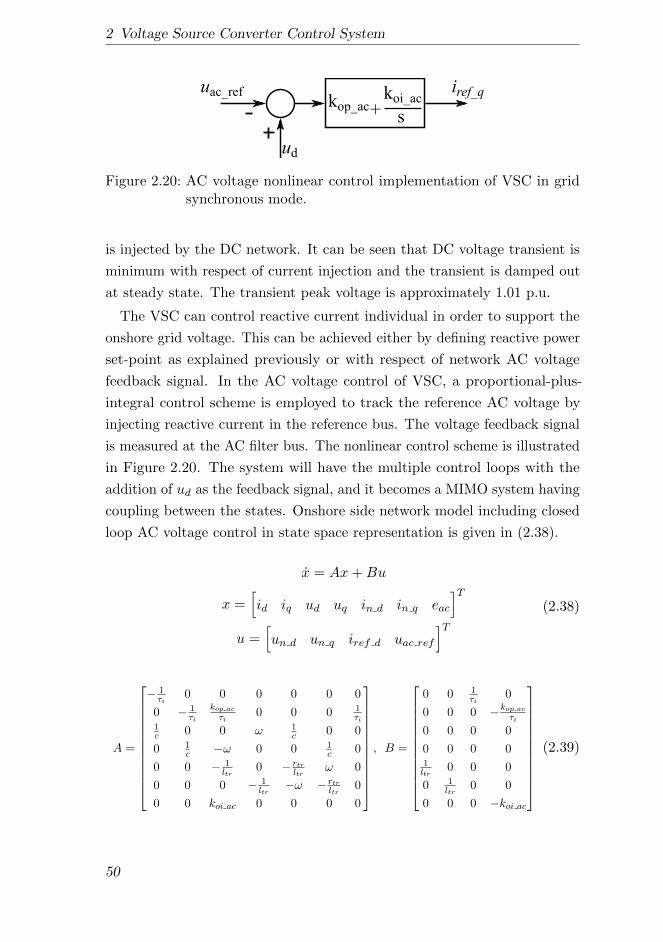
2 Voltage Source Converter Control System

koi_ac

skop_ac+

uac_ref

ud

iref_q

Figure 2.20: AC voltage nonlinear control implementation of VSC in gridsynchronous mode.

is injected by the DC network. It can be seen that DC voltage transient is

minimum with respect of current injection and the transient is damped out

at steady state. The transient peak voltage is approximately 1.01 p.u.

The VSC can control reactive current individual in order to support the

onshore grid voltage. This can be achieved either by defining reactive power

set-point as explained previously or with respect of network AC voltage

feedback signal. In the AC voltage control of VSC, a proportional-plus-

integral control scheme is employed to track the reference AC voltage by

injecting reactive current in the reference bus. The voltage feedback signal

is measured at the AC filter bus. The nonlinear control scheme is illustrated

in Figure 2.20. The system will have the multiple control loops with the

addition of ud as the feedback signal, and it becomes a MIMO system having

coupling between the states. Onshore side network model including closed

loop AC voltage control in state space representation is given in (2.38).

x = Ax+Bu

x =[id iq ud uq in d in q eac

]Tu =

[un d un q iref d uac ref

]T (2.38)

A =

− 1τi

0 0 0 0 0 0

0 − 1τi

kop ac

τi0 0 0 1

τi1c 0 0 ω 1

c 0 0

0 1c −ω 0 0 1

c 0

0 0 − 1ltr

0 − rtrltr

ω 0

0 0 0 − 1ltr

−ω − rtrltr

0

0 0 koi ac 0 0 0 0

, B =

0 0 1τi

0

0 0 0 −kop ac

τi

0 0 0 0

0 0 0 01ltr

0 0 0

0 1ltr

0 0

0 0 0 −koi ac

(2.39)

50

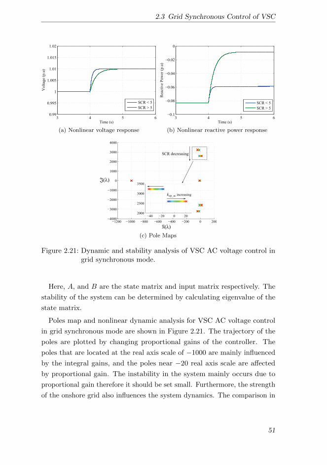
2.3 Grid Synchronous Control of VSC

3 4 5 60.99

0.995

1

1.005

1.01

1.015

1.02

Time (s)

Vo

ltag

e (p

.u)

SCR < 5

SCR > 5

(a) Nonlinear voltage response

3 4 5 60.1

0.08

0.06

0.04

0.02

0

Time (s)

Rea

ctiv

e P

ow

er (

p.u

)

SCR < 5

SCR > 5

(b) Nonlinear reactive power response

1200 1000 800 600 400 200 0 2004000

3000

2000

1000

0

1000

2000

3000

4000

40 20 0 202000

2500

3000

3500

( )

( )

SCR decreasing

kop_ac increasing

(c) Pole Maps

Figure 2.21: Dynamic and stability analysis of VSC AC voltage control ingrid synchronous mode.

Here, A, and B are the state matrix and input matrix respectively. The

stability of the system can be determined by calculating eigenvalue of the

state matrix.

Poles map and nonlinear dynamic analysis for VSC AC voltage control

in grid synchronous mode are shown in Figure 2.21. The trajectory of the

poles are plotted by changing proportional gains of the controller. The

poles that are located at the real axis scale of −1000 are mainly influenced

by the integral gains, and the poles near −20 real axis scale are affected

by proportional gain. The instability in the system mainly occurs due to

proportional gain therefore it should be set small. Furthermore, the strength

of the onshore grid also influences the system dynamics. The comparison in

51

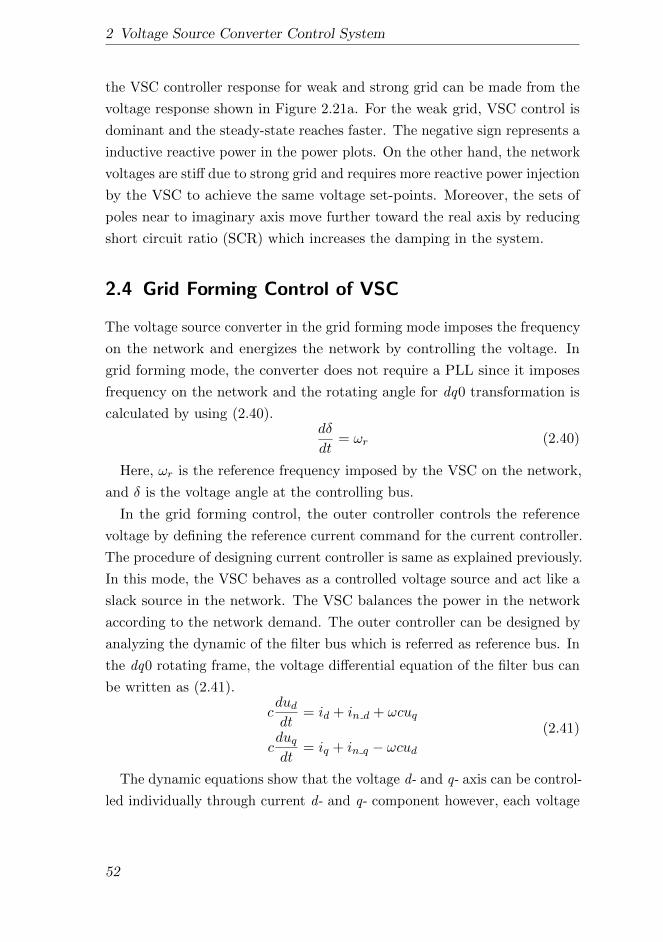
2 Voltage Source Converter Control System

the VSC controller response for weak and strong grid can be made from the

voltage response shown in Figure 2.21a. For the weak grid, VSC control is

dominant and the steady-state reaches faster. The negative sign represents a

inductive reactive power in the power plots. On the other hand, the network

voltages are stiff due to strong grid and requires more reactive power injection

by the VSC to achieve the same voltage set-points. Moreover, the sets of

poles near to imaginary axis move further toward the real axis by reducing

short circuit ratio (SCR) which increases the damping in the system.

2.4 Grid Forming Control of VSC

The voltage source converter in the grid forming mode imposes the frequency

on the network and energizes the network by controlling the voltage. In

grid forming mode, the converter does not require a PLL since it imposes

frequency on the network and the rotating angle for dq0 transformation is

calculated by using (2.40).dδ

dt= ωr (2.40)

Here, ωr is the reference frequency imposed by the VSC on the network,

and δ is the voltage angle at the controlling bus.

In the grid forming control, the outer controller controls the reference

voltage by defining the reference current command for the current controller.

The procedure of designing current controller is same as explained previously.

In this mode, the VSC behaves as a controlled voltage source and act like a

slack source in the network. The VSC balances the power in the network

according to the network demand. The outer controller can be designed by

analyzing the dynamic of the filter bus which is referred as reference bus. In

the dq0 rotating frame, the voltage differential equation of the filter bus can

be written as (2.41).

cduddt

= id + in d + ωcuq

cduqdt

= iq + in q − ωcud(2.41)

The dynamic equations show that the voltage d- and q- axis can be control-

led individually through current d- and q- component however, each voltage

52

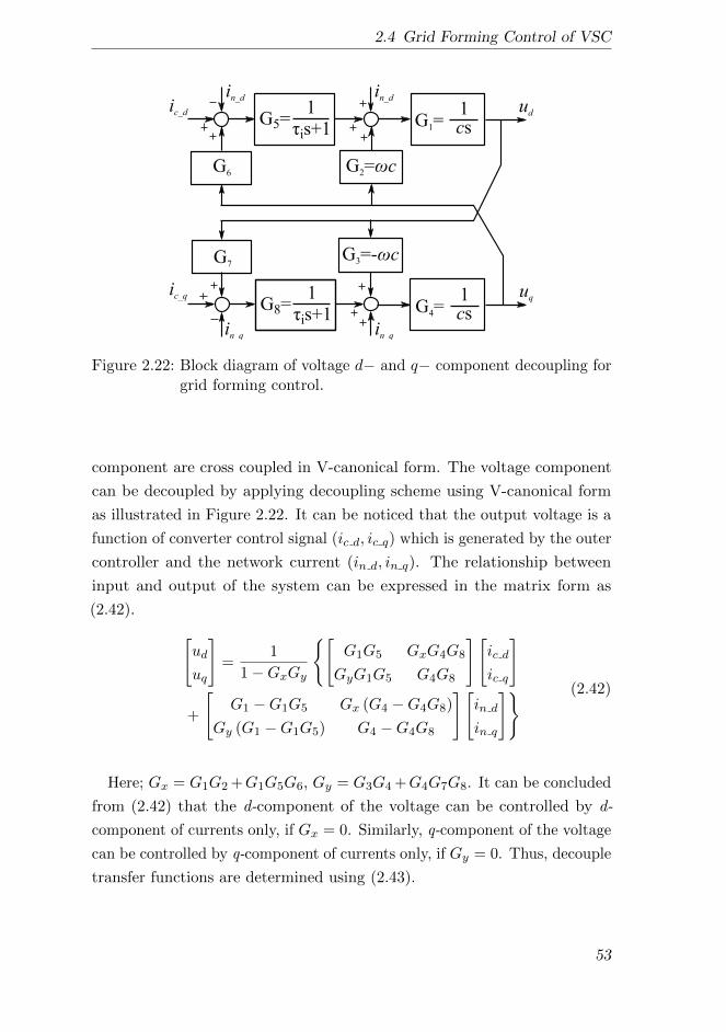
2.4 Grid Forming Control of VSC

G2= c

ud

uq

in_d

in_q

ic_d

ic_q

1

csG1=

G3=- c

G6

G7

G5=is+1

1

1

csG4=G8=

is+1

1

in_d

in_q

Figure 2.22: Block diagram of voltage d− and q− component decoupling forgrid forming control.

component are cross coupled in V-canonical form. The voltage component

can be decoupled by applying decoupling scheme using V-canonical form

as illustrated in Figure 2.22. It can be noticed that the output voltage is a

function of converter control signal (ic d, ic q) which is generated by the outer

controller and the network current (in d, in q). The relationship between

input and output of the system can be expressed in the matrix form as

(2.42). [ud

uq

]=

1

1−GxGy

[G1G5 GxG4G8

GyG1G5 G4G8

][ic d

ic q

]

+

[G1 −G1G5 Gx (G4 −G4G8)

Gy (G1 −G1G5) G4 −G4G8

][in d

in q

] (2.42)

Here; Gx = G1G2 +G1G5G6, Gy = G3G4 +G4G7G8. It can be concluded

from (2.42) that the d-component of the voltage can be controlled by d-

component of currents only, if Gx = 0. Similarly, q-component of the voltage

can be controlled by q-component of currents only, if Gy = 0. Thus, decouple

transfer functions are determined using (2.43).

53

2 Voltage Source Converter Control System

1

is+1koi_rs

kop_r +ur(s) 1

cs

is+1is

u(s)

in(s)

ic(s)

(a) Stability model

kop_r+koi_rs

c

+-

-+

+

+

+

-

in_d

in_q

ud

uq

uref_d

uref_q

iref_d

s+1ti( )

s+1ti( )

iref_q

ic_d

ic_q

c

-

-

kop_r+koi_rs

(b) Nonlinear implementation model

Figure 2.23: VSC Closed loop block diagram of grid forming control.

G6 =−G2

G5= −w · c1 · (τis+ 1)

G7 =−G3

G8= w · c1 · (τis+ 1)

(2.43)

Open loop voltage model including decouple transfer function in state-

space representation is given in (2.44).id

iq

ud

uq

=

− 1τi−ω ω2c −ωc

τi

ω − 1τi

ωcτi

ω2c1c 0 0 ω

0 1c −ω 0

id

iq

ud

uq

+

1τi

0 − 1τi−ω

0 1τi

ω − 1τi

0 0 1c 0

0 0 0 1c

ic d

ic q

in d

in q

(2.44)

Eigenvalues of the state matrix are calculated to determine the poles of

the system. From (2.45), it can be seen that the system has four poles, two

54

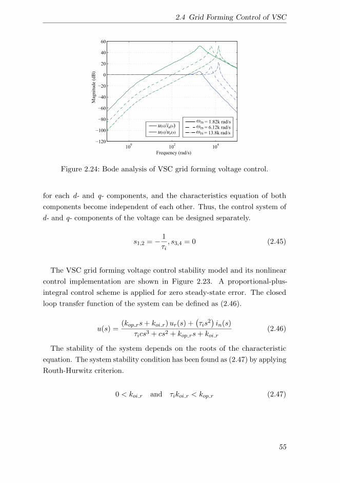
2.4 Grid Forming Control of VSC

100

102

104

120

100

80

60

40

20

0

20

40

60

Mag

nit

ude

(dB

)

Frequency (rad/s)

u(s)/ur(s)

u(s)/in(s)rs = 1.82k rad/s

rs = 6.12k rad/srs = 13.8k rad/s

Figure 2.24: Bode analysis of VSC grid forming voltage control.

for each d- and q- components, and the characteristics equation of both

components become independent of each other. Thus, the control system of

d- and q- components of the voltage can be designed separately.

s1,2 = − 1

τi, s3,4 = 0 (2.45)

The VSC grid forming voltage control stability model and its nonlinear

control implementation are shown in Figure 2.23. A proportional-plus-

integral control scheme is applied for zero steady-state error. The closed

loop transfer function of the system can be defined as (2.46).

u(s) =(kop rs+ koi r)ur(s) +

(τis

2)in(s)

τics3 + cs2 + kop rs+ koi r(2.46)

The stability of the system depends on the roots of the characteristic

equation. The system stability condition has been found as (2.47) by applying

Routh-Hurwitz criterion.

0 < koi r and τikoi r < kop r (2.47)

55

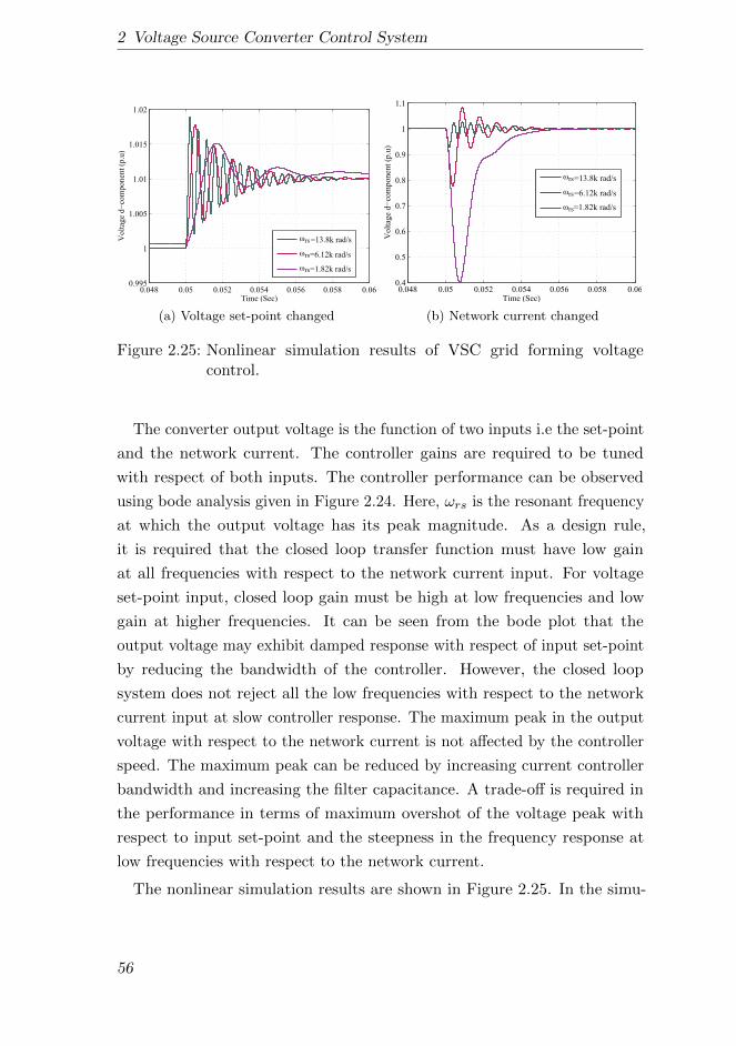
2 Voltage Source Converter Control System

0.048 0.05 0.052 0.054 0.056 0.058 0.060.995

1

1.005

1.01

1.015

1.02

Time (Sec)

Volt

age

dco

mponen

t (p

.u)

rs=13.8k rad/s

rs=6.12k rad/s

rs=1.82k rad/s

(a) Voltage set-point changed

0.048 0.05 0.052 0.054 0.056 0.058 0.060.4

0.5

0.6

0.7

0.8

0.9

1

1.1

Time (Sec)

Volt

age

dco

mpo

nen

t (p

.u)

rs=13.8k rad/s

rs=6.12k rad/s

rs=1.82k rad/s

(b) Network current changed

Figure 2.25: Nonlinear simulation results of VSC grid forming voltagecontrol.

The converter output voltage is the function of two inputs i.e the set-point

and the network current. The controller gains are required to be tuned

with respect of both inputs. The controller performance can be observed

using bode analysis given in Figure 2.24. Here, ωrs is the resonant frequency

at which the output voltage has its peak magnitude. As a design rule,

it is required that the closed loop transfer function must have low gain

at all frequencies with respect to the network current input. For voltage

set-point input, closed loop gain must be high at low frequencies and low

gain at higher frequencies. It can be seen from the bode plot that the

output voltage may exhibit damped response with respect of input set-point

by reducing the bandwidth of the controller. However, the closed loop

system does not reject all the low frequencies with respect to the network

current input at slow controller response. The maximum peak in the output

voltage with respect to the network current is not affected by the controller

speed. The maximum peak can be reduced by increasing current controller

bandwidth and increasing the filter capacitance. A trade-off is required in

the performance in terms of maximum overshot of the voltage peak with

respect to input set-point and the steepness in the frequency response at

low frequencies with respect to the network current.

The nonlinear simulation results are shown in Figure 2.25. In the simu-

56

2.5 VSC Substation Models for System Studies

i

Udc

l r

c

Cdc

Il Idc

inuv u un

kp+kis

kp+kis

+

-+

+-

+

-

++

+

T-1( (t))id

iq

ud

uq

l

l

iref_d

iref_q

uv_d

uv_q

uv_abc

kop_r+koi_rs

c

+-

-+

+

+

+

-

in_d

in_q

ud

uq

uref_d

uref_q

s+1ti( )

s+1ti( )

ic_d

ic_q

c

-

-

kop_r+koi_rs

T( (t))T( (t))T( (t))in u i1

sr

(t) uduq

idiq

in_d

in_q

110kVLL 150kVLL

+/-150kV

112MVA

Figure 2.26: Offshore substation configuration of VSC HVDC transmissionsystem.

lation, the network current is changed from zero to 1.0 p.u in active load

and the voltage set-point is changed from 1.0 p.u to 1.01 p.u. Note that

the performance has been analyzed with respect to both inputs by applying

step change one at a time. It is clear from the result that faster controller

response increases the peak overshoot and high oscillation in the output

voltage while changing input set-point. High controller gain value provide

better performance against high rate of change of network current. Further,

the offshore grid code may specify the maximum rate of change of power in

the offshore network to avoid large voltage deviation during transient.

2.5 VSC Substation Models for System Studies

In this thesis, three voltage source converter based substation configurations

are build to perform different case studies. An overview of these configu-

rations are given in this section. The VSC substation network elements

value and its control gain settings are also listed. The studies have been

performed using these parameters otherwise stated explicitly in each chapter.

Further, the control system is designed in p.u system to be able to adapt for

57

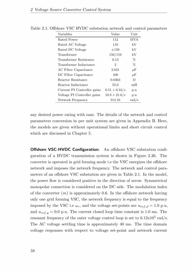
2 Voltage Source Converter Control System

Table 2.1: Offshore VSC HVDC substation network and control parameters

Variables Value Unit

Rated Power 112 MVA

Rated AC Voltage 110 kV

Rated DC Voltage ±150 kV

Transformer 150/110 kV

Transformer Resistance 0.12 %

Transformer Inductance 2 %

AC Filter Capacitance 2.631 µF

DC Filter Capacitance 100 µF

Reactor Resistance 0.0363 Ω

Reactor Inductance 55.0 mH

Current PI Controller gains 0.51 + 0.34/s p.u

Voltage PI Controller gains 10.8 + 21.6/s p.u

Network Frequency 314.16 rad/s

any desired power rating with ease. The details of the network and control

parameters conversion in per unit system are given in Appendix B. Here,

the models are given without operational limits and short circuit control

which are discussed in Chapter 5.

Offshore VSC-HVDC Configuration: An offshore VSC substation confi-

guration of a HVDC transmission system is shown in Figure 2.26. The

converter is operated in grid forming mode i.e the VSC energizes the offshore

network and imposes the network frequency. The network and control para-

meters of an offshore VSC substation are given in Table 2.1. In the model,

the power flow is considered positive in the direction of arrow. Symmetrical

monopolar connection is considered on the DC side. The modulation index

of the converter (m) is approximately 0.6. In the offshore network having

only one grid forming VSC, the network frequency is equal to the frequency

imposed by the VSC i.e ωr, and the voltage set-points are uref d = 1.0 p.u,

and uref q = 0.0 p.u. The current closed loop time constant is 1.0 ms. The

resonant frequency of the outer voltage control loop is set to 6.12x103 rad/s.

The AC voltage settling time is approximately 40 ms. The time domain

voltage responses with respect to voltage set-point and network current

58

2.5 VSC Substation Models for System Studies

i

Udc

lg rg

Cdc

Il Idc

uv u un

kp+kis

kp+kis

+

-+

+-

+

-

++

+

T-1( (t))

id

iq

ud

uq

l

l

iref_d

iref_q

uv_d

uv_q

uv_abc

T( (t))T( (t))u i

(t) uduq

idiq

110kVLL 220kVLL

112MVA

g

koi_dc

skop_dc +

Udc_ref

Udc

Il

+

+

PLLu

+

p

q

idq

udqp

q udq idq=s

gggg

gg

g

g

cg

ud

uac_ref koi_ac

skop_ac +g

g

--

-

Figure 2.27: Onshore substation configuration of VSC HVDC transmissionsystem.

infeed are shown in previous section. According to the analysis, a voltage

dip up to 0.8 p.u will occur when the step change in the network current is

applied from zero to rated value.

The grid forming control is further extended in the next chapter for the

offshore AC network control interconnecting several grid forming VSCs.

Onshore VSC-HVDC Configuration: The configuration of an onshore VSC

substation of a HVDC transmission system is shown in Figure 2.27. The

VSC is synchronized with the grid frequency thus requires a PLL. The outer

controller operates in the DC voltage and AC voltage control mode. The

onshore converter is controlling the DC voltage to balance the DC link.

In the point-to-point configuration of HVDC transmission system, the DC

voltage control is based on PI regulator as explained in previous section.

While the DC voltage control has proportional regulator in multiterminal

HVDC transmission system which is explained in Chapter 6. Also, an

AC voltage control mode is set in order to support the onshore AC grid

voltages. The set-points for AC and DC voltages are uac ref = 1.0 p.u and

Udc ref = 1.0 p.u respectively. The network and control parameters are given

59

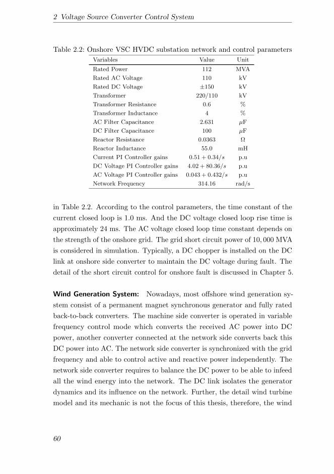
2 Voltage Source Converter Control System

Table 2.2: Onshore VSC HVDC substation network and control parameters

Variables Value Unit

Rated Power 112 MVA

Rated AC Voltage 110 kV

Rated DC Voltage ±150 kV

Transformer 220/110 kV

Transformer Resistance 0.6 %

Transformer Inductance 4 %

AC Filter Capacitance 2.631 µF

DC Filter Capacitance 100 µF

Reactor Resistance 0.0363 Ω

Reactor Inductance 55.0 mH

Current PI Controller gains 0.51 + 0.34/s p.u

DC Voltage PI Controller gains 4.02 + 80.36/s p.u

AC Voltage PI Controller gains 0.043 + 0.432/s p.u

Network Frequency 314.16 rad/s

in Table 2.2. According to the control parameters, the time constant of the

current closed loop is 1.0 ms. And the DC voltage closed loop rise time is

approximately 24 ms. The AC voltage closed loop time constant depends on

the strength of the onshore grid. The grid short circuit power of 10, 000 MVA

is considered in simulation. Typically, a DC chopper is installed on the DC

link at onshore side converter to maintain the DC voltage during fault. The

detail of the short circuit control for onshore fault is discussed in Chapter 5.

Wind Generation System: Nowadays, most offshore wind generation sy-

stem consist of a permanent magnet synchronous generator and fully rated

back-to-back converters. The machine side converter is operated in variable

frequency control mode which converts the received AC power into DC

power, another converter connected at the network side converts back this

DC power into AC. The network side converter is synchronized with the grid

frequency and able to control active and reactive power independently. The

network side converter requires to balance the DC power to be able to infeed

all the wind energy into the network. The DC link isolates the generator

dynamics and its influence on the network. Further, the detail wind turbine

model and its mechanic is not the focus of this thesis, therefore, the wind

60

2.5 VSC Substation Models for System Studies

i

Udc

lw rw

Cdc

Il Idc

uv u un

kp+kis

kp+kis

+

-+

+-

+

-

++

+

T-1( (t))

id

iq

ud

uq

l

l

iref_d

iref_q

uv_d

uv_q

uv_abc

T( (t))T( (t))u i

(t) uduq

idiq

900VLL 33kVLL

6.3MVA

w

koi_dc

skop_dc +

Udc_ref

Udc

Il

+

+

PLLu

qsetkois

kop +

q+

p

q

idq

udqp

q udq idq=s

ww

ww

ww

ww

w

w

Iwind

Figure 2.28: Grid side wind turbine VSC substation configuration.

generation system contains only network side converter in the study cases.

The wind generation substation configuration is shown in Figure 2.28.

The network and control parameters for the wind generation system are

given in Table 2.3. A step-up transformer is installed to connect the wind

model with the offshore wind power plant array. Typically, the wind power

plant array consist of medium voltage cables of 33 kV level. The converter is

set to control the DC voltage and the reactive power. According to the control

system design, the rise time of the DC voltage control loop is approximately

24 ms, and the DC voltage set-point is defined as Udc ref = 1.0 p.u. The time

constant of the reactive power control loop is approximately 20 ms. Moreover,

the reactive power set-point can be defined according the reactive power

support required by the network. The current closed loop time constant is

also set to 1.0 ms.

The wind energy infeed by the wind turbine is modeled as constant current

source. The wind energy variation can be incorporated in the network study

by using wind power to speed profile. Again, a DC chopper is required on

the DC link to control the voltage during fault. The detail of the chopper

control is explained in the Chapter 5.

61

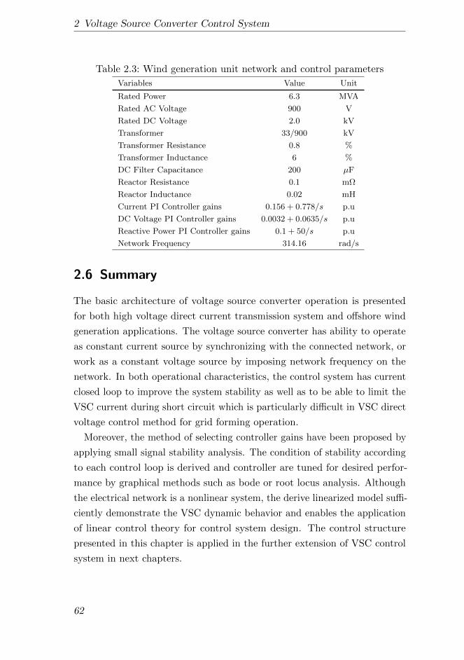
2 Voltage Source Converter Control System

Table 2.3: Wind generation unit network and control parameters

Variables Value Unit

Rated Power 6.3 MVA

Rated AC Voltage 900 V

Rated DC Voltage 2.0 kV

Transformer 33/900 kV

Transformer Resistance 0.8 %

Transformer Inductance 6 %

DC Filter Capacitance 200 µF

Reactor Resistance 0.1 mΩ

Reactor Inductance 0.02 mH

Current PI Controller gains 0.156 + 0.778/s p.u

DC Voltage PI Controller gains 0.0032 + 0.0635/s p.u

Reactive Power PI Controller gains 0.1 + 50/s p.u

Network Frequency 314.16 rad/s

2.6 Summary

The basic architecture of voltage source converter operation is presented

for both high voltage direct current transmission system and offshore wind

generation applications. The voltage source converter has ability to operate

as constant current source by synchronizing with the connected network, or

work as a constant voltage source by imposing network frequency on the

network. In both operational characteristics, the control system has current

closed loop to improve the system stability as well as to be able to limit the

VSC current during short circuit which is particularly difficult in VSC direct

voltage control method for grid forming operation.

Moreover, the method of selecting controller gains have been proposed by

applying small signal stability analysis. The condition of stability according

to each control loop is derived and controller are tuned for desired perfor-

mance by graphical methods such as bode or root locus analysis. Although

the electrical network is a nonlinear system, the derive linearized model suffi-

ciently demonstrate the VSC dynamic behavior and enables the application

of linear control theory for control system design. The control structure

presented in this chapter is applied in the further extension of VSC control

system in next chapters.

62

3 Offshore Network having Grid

Forming VSC-HVDC System

In this chapter, a concept of an offshore grid is introduced to interconnect

several offshore wind power plants with different onshore grids using VSC-

HVDC transmission system. The VSC grid forming control presented

in previous chapter has been extended to form an offshore AC network.

Frequency and voltage droop schemes have been implemented to control

the sharing of active and reactive power among VSC-HVDC transmission

systems. Furthermore, the voltage droop control provides additional degree

of freedom to manage the reactive power in the offshore AC network. Later in

the chapter, an optimization algorithm is developed to optimize the reactive

power flow in order to minimize the losses in the network2,3.

3.1 Introduction

Renewable energy is becoming a universally adopted primary source of

energy. A breakthrough in advanced power transmission system technologies,

specially in the power electronics devices, have enabled the installation of

renewable generation units at remote location. Wind energy among other

renewable sources has been a main focus in the last decade, particularly

offshore. Up to the mid of 2016, 3344 offshore wind turbines with a combined

power of 11.54 GW are installed in European waters [98].

2This chapter is based on the following publications:M. Raza, K. Schoenleber, and O. Gomis-Bellmunt, “Droop control design of multi-VSCsystem for offshore network to integrate wind energy”. Energies (MDPI), 9(10):826,oct 2016, doi: 10.3390/en9100826.

3M. Raza, C. Collados, and O. Gomis-Bellmunt, “Reactive power management in an off-shore ac network having multiple voltage source converters”. Applied Energy (Elseiver),206:793-803, nov 2017. ISSN 0306-2619. doi: 10.1016/j.apenergy.2017.08.182.

63

3 Offshore Network having Grid Forming VSC-HVDC System

The most common export system of an offshore wind power plant is the

high voltage alternating current (HVAC) cables link with an onshore grid,

typically at the voltage level of 150 kV. The HVAC export system is well

established technology as well as it provides grid forming interconnection to

offshore network. However, the HVAC cables have high effective capacitance

that limits the transmission of large active power over the long distance

through Sea, typically limited up to 90 km for 100 MW [21]. The voltage

source converter (VSC) based high voltage direct current (HVDC) transmis-

sion system eliminate the power export limitation due to the cable capacitive

effect and it has an ability to form the offshore network. However, the

current rating of the switching devices (IGBTs) restrains the power transfer

capacity.

Many experts are foreseeing the need of having offshore grid for better

trade and integration of large offshore wind energy generation. In [99], the

impact of an offshore grid on the European energy market has been studied

considering several technical concepts for grid connection. One of the concept

in the offshore grid is to create a multiterminal (MT) HVDC system to

connect the several offshore wind power plants and integrate them with

different onshore grids. However, the DC circuit breaker based protection

scheme in the MTDC system increases the overall development cost [60, 65].

On the contrary, an offshore AC network formed by connecting wind power

plants using HVAC cables and then using several VSC-HVDC systems in

a point-to-point configuration to link with different onshore grids provides

advantage to not to employee DC circuit breaker and the protection scheme

can be applied similar to conventional AC system. An offshore AC network

act as a mediator among several wind power plants and different countries

grids. In [22], several options of forming offshore AC network are considered

by connecting wind power plants center collection points with each other

using medium or high voltage AC cable (normally, at 150 kV). This offshore

AC network is then connected with the main grids of neighboring countries

via VSC-HVDC system. Offshore wind power plants that are far from

shore and are within the vicinity of 20 km from each other are economically

suitable to form an offshore AC network [100].

In a stand alone network such as an offshore AC network, the VSC-HVDC

64

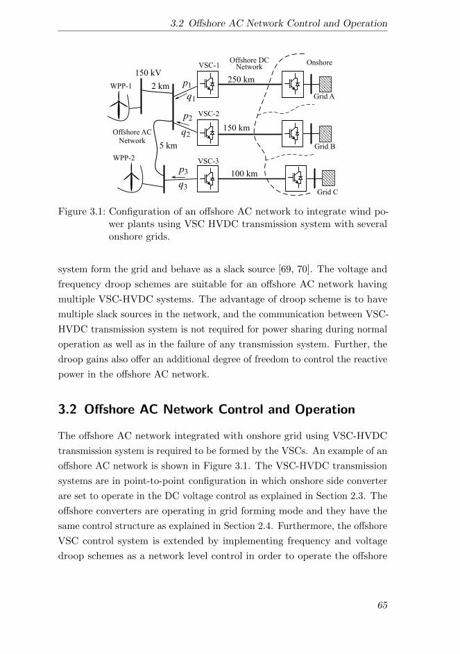
3.2 Offshore AC Network Control and Operation

q1

Onshore

Grid A

Grid B

Grid C

Offshore DCNetworkVSC-1

VSC-2

VSC-3

Offshore AC

Network

WPP-1

WPP-2

2 km

5 km

150 kV250 km

150 km

100 km

p1

q2

p2

q3

p3

Figure 3.1: Configuration of an offshore AC network to integrate wind po-wer plants using VSC HVDC transmission system with severalonshore grids.

system form the grid and behave as a slack source [69, 70]. The voltage and

frequency droop schemes are suitable for an offshore AC network having

multiple VSC-HVDC systems. The advantage of droop scheme is to have

multiple slack sources in the network, and the communication between VSC-

HVDC transmission system is not required for power sharing during normal

operation as well as in the failure of any transmission system. Further, the

droop gains also offer an additional degree of freedom to control the reactive

power in the offshore AC network.

3.2 Offshore AC Network Control and Operation

The offshore AC network integrated with onshore grid using VSC-HVDC

transmission system is required to be formed by the VSCs. An example of an

offshore AC network is shown in Figure 3.1. The VSC-HVDC transmission

systems are in point-to-point configuration in which onshore side converter

are set to operate in the DC voltage control as explained in Section 2.3. The

offshore converters are operating in grid forming mode and they have the

same control structure as explained in Section 2.4. Furthermore, the offshore

VSC control system is extended by implementing frequency and voltage

droop schemes as a network level control in order to operate the offshore

65

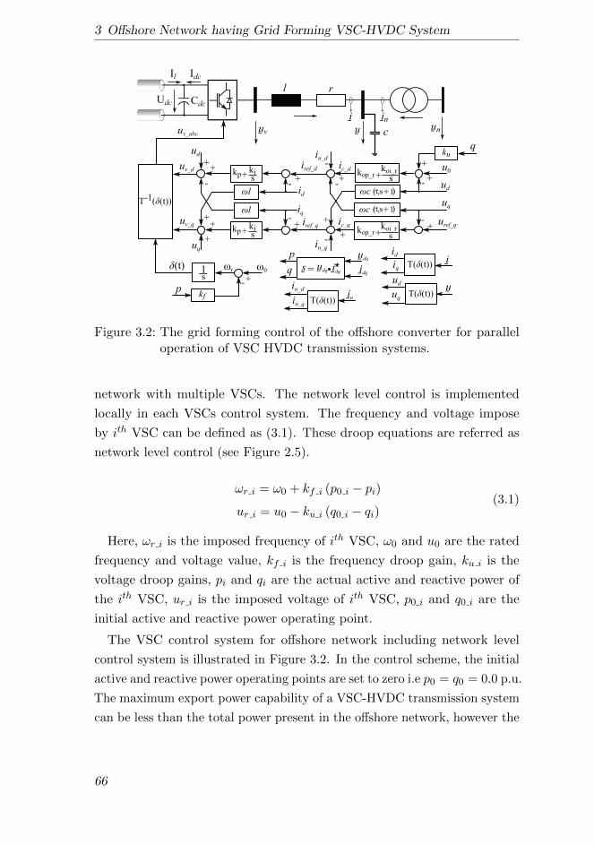
3 Offshore Network having Grid Forming VSC-HVDC System

i

Udc

l r

c

Cdc

Il Idc

inuv u un

kp+kis

kp+kis

+

-+

+-

+

-

++

+

T-1( (t))id

iq

ud

uq

l

l

iref_d

iref_q

uv_d

uv_q

uv_abc

kop_r+koi_rs

c

+-

-+

+

+

+

-

in_d

in_q

ud

uq

u0

uref_q

s+1ti( )

s+1ti( )

ic_d

ic_q

c

-

-

kop_r+koi_rs

T( (t))

T( (t))T( (t))

inu

i1s

r(t)

uduq

idiq

in_d

in_qkf

p-+

0 idq

udqp

q udq idq=s

ku+

q

Figure 3.2: The grid forming control of the offshore converter for paralleloperation of VSC HVDC transmission systems.

network with multiple VSCs. The network level control is implemented

locally in each VSCs control system. The frequency and voltage impose

by ith VSC can be defined as (3.1). These droop equations are referred as

network level control (see Figure 2.5).

ωr i = ω0 + kf i (p0 i − pi)

ur i = u0 − ku i (q0 i − qi)(3.1)

Here, ωr i is the imposed frequency of ith VSC, ω0 and u0 are the rated

frequency and voltage value, kf i is the frequency droop gain, ku i is the

voltage droop gains, pi and qi are the actual active and reactive power of

the ith VSC, ur i is the imposed voltage of ith VSC, p0 i and q0 i are the

initial active and reactive power operating point.

The VSC control system for offshore network including network level

control system is illustrated in Figure 3.2. In the control scheme, the initial

active and reactive power operating points are set to zero i.e p0 = q0 = 0.0 p.u.

The maximum export power capability of a VSC-HVDC transmission system

can be less than the total power present in the offshore network, however the

66

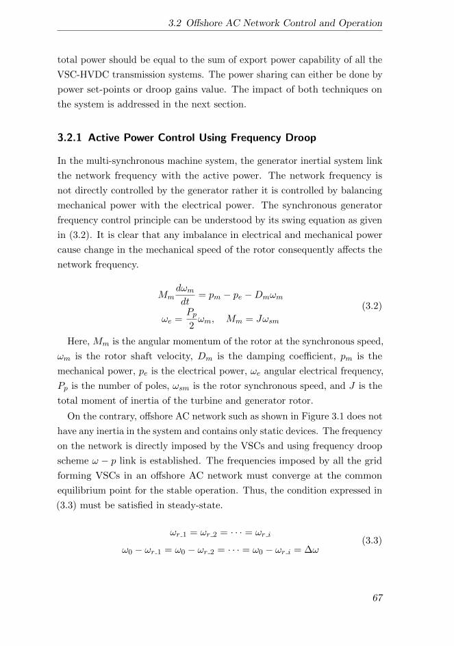
3.2 Offshore AC Network Control and Operation

total power should be equal to the sum of export power capability of all the

VSC-HVDC transmission systems. The power sharing can either be done by

power set-points or droop gains value. The impact of both techniques on

the system is addressed in the next section.

3.2.1 Active Power Control Using Frequency Droop

In the multi-synchronous machine system, the generator inertial system link

the network frequency with the active power. The network frequency is

not directly controlled by the generator rather it is controlled by balancing

mechanical power with the electrical power. The synchronous generator

frequency control principle can be understood by its swing equation as given

in (3.2). It is clear that any imbalance in electrical and mechanical power

cause change in the mechanical speed of the rotor consequently affects the

network frequency.

Mmdωmdt

= pm − pe −Dmωm

ωe =Pp2ωm, Mm = Jωsm

(3.2)

Here, Mm is the angular momentum of the rotor at the synchronous speed,

ωm is the rotor shaft velocity, Dm is the damping coefficient, pm is the

mechanical power, pe is the electrical power, ωe angular electrical frequency,

Pp is the number of poles, ωsm is the rotor synchronous speed, and J is the

total moment of inertia of the turbine and generator rotor.

On the contrary, offshore AC network such as shown in Figure 3.1 does not

have any inertia in the system and contains only static devices. The frequency

on the network is directly imposed by the VSCs and using frequency droop

scheme ω − p link is established. The frequencies imposed by all the grid

forming VSCs in an offshore AC network must converge at the common

equilibrium point for the stable operation. Thus, the condition expressed in

(3.3) must be satisfied in steady-state.

ωr 1 = ωr 2 = · · · = ωr i

ω0 − ωr 1 = ω0 − ωr 2 = · · · = ω0 − ωr i = ∆ω(3.3)

67

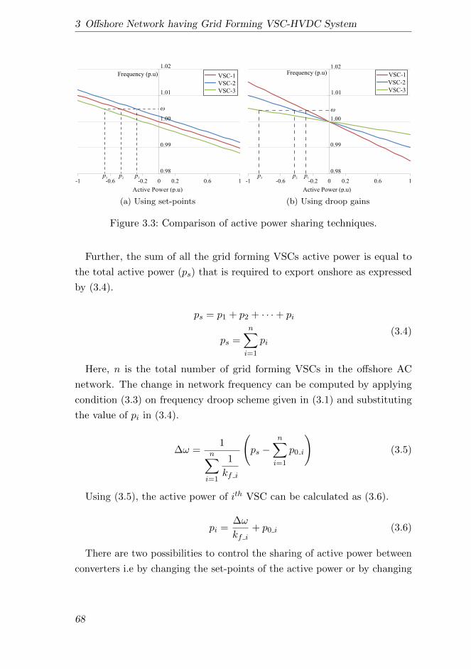
3 Offshore Network having Grid Forming VSC-HVDC System

0.98

0.99

1.00

1.01

1.02

-1 -0.6 -0.2 0.2 0.6 1

Frequency (p.u)

Active Power (p.u)

p1p2p3

VSC-1

VSC-2

VSC-3

0

(a) Using set-points

0.98

0.99

1.00

1.01

1.02

-1 -0.6 -0.2 0.2 0.6 1

Frequency (p.u)

Active Power (p.u)

p1p2p3

VSC-1

VSC-2

VSC-3

0

(b) Using droop gains

Figure 3.3: Comparison of active power sharing techniques.

Further, the sum of all the grid forming VSCs active power is equal to

the total active power (ps) that is required to export onshore as expressed

by (3.4).

ps = p1 + p2 + · · ·+ pi

ps =

n∑i=1

pi(3.4)

Here, n is the total number of grid forming VSCs in the offshore AC

network. The change in network frequency can be computed by applying

condition (3.3) on frequency droop scheme given in (3.1) and substituting

the value of pi in (3.4).

∆ω =1

n∑i=1

1

kf i

(ps −

n∑i=1

p0 i

)(3.5)

Using (3.5), the active power of ith VSC can be calculated as (3.6).

pi =∆ω

kf i+ p0 i (3.6)

There are two possibilities to control the sharing of active power between

converters i.e by changing the set-points of the active power or by changing

68

3.2 Offshore AC Network Control and Operation

0.8 1.0 1.2 1.4 1.6 1.8

1.0000

1.0005

1.0010

1.0015

1.0020

1.0025

Time (sec)

Fre

quen

cy(p

.u)

1

2

3

(a) VSCs frequencies

0.8 1.0 1.2 1.4 1.6 1.80.8

0.6

0.4

0.2

0.0

0.2

Time (sec)

Act

ive

Pow

er (

p.u

)

p1

p2

p3

(b) VSCs active powers

Figure 3.4: Illustration of frequency and active power distribution usingset-points.

the droop gains value. The comparison between these two techniques is

shown in Figure 3.3.

Active Power Sharing Using Set-points: In the first method, the distribu-

tion of the active power among converters is achieved by assigning different

active power set-points while keeping droop gains value for all grid forming

VSCs equal.

p0 1 6= p0 2 6= · · · 6= p0 i

kf 1 = kf 2 = · · · = kf i = kf 6= 0(3.7)

Thus, the steady-state change in network frequency and the ith VSC active

power can be calculated as (3.8) by applying condition given in (3.7) on

(3.5) and (3.6).

∆ω =kfn

(ps −

n∑i=1

p0 i

)

pi =1

n

ps − n∑j=1j 6=i

p0 j

+

(n− 1

n

)p0 i

(3.8)

69

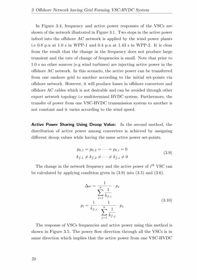
3 Offshore Network having Grid Forming VSC-HVDC System

In Figure 3.4, frequency and active power responses of the VSCs are

shown of the network illustrated in Figure 3.1. Two steps in the active power

infeed into the offshore AC network is applied by the wind power plants

i.e 0.8 p.u at 1.0 s in WPP-1 and 0.4 p.u at 1.43 s in WPP-2. It is clear

from the result that the change in the frequency does not produce large

transient and the rate of change of frequencies is small. Note that prior to

1.0 s no other sources (e.g wind turbines) are injecting active power in the

offshore AC network. In this scenario, the active power can be transferred

from one onshore grid to another according to the initial set-points via

offshore network. However, it will produce losses in offshore converters and

offshore AC cables which is not desirable and can be avoided through other

export network topology i.e multiterminal HVDC system. Furthermore, the

transfer of power from one VSC-HVDC transmission system to another is

not constant and it varies according to the wind speed.

Active Power Sharing Using Droop Value: In the second method, the

distribution of active power among converters is achieved by assigning

different droop values while having the same active power set-points.

p0 1 = p0 2 = · · · = p0 i = 0

kf 1 6= kf 2 6= · · · 6= kf i 6= 0(3.9)

The change in the network frequency and the active power of ith VSC can

be calculated by applying condition given in (3.9) into (3.5) and (3.6).

∆ω =1

n∑i=1

1

kf i

· ps

pi =1

kf i· 1

n∑j=1

1

kf j

· ps(3.10)

The response of VSCs frequencies and active power using this method is

shown in Figure 3.5. The power flow direction through all the VSCs is in

same direction which implies that the active power from one VSC-HVDC

70

3.2 Offshore AC Network Control and Operation

0.8 1.0 1.2 1.4 1.6 1.80.9999

1.0000

1.0001

1.0002

1.0003

1.0004

1.0005

1.0006

1.0007

1.0008

1.0009

1.0010

Time (sec)

Fre

quen

cy (

p.u

)

1

2

3

(a) VSCs frequencies

0.8 1.0 1.2 1.4 1.6 1.80.8

0.7

0.6

0.5

0.4

0.3

0.2

0.1

0.0

0.1

Time (sec)

Act

ive

Pow

er (

p.u

)

p1

p2

p3

(b) VSCs active powers

Figure 3.5: Illustration of frequency response and active power distributionusing droop gains of an offshore AC network.

transmission system will not be injected to another. Only the active power

infeed by the wind power plants will be exported to onshore grids. Such an

operation is like the slack source in the electrical network which is desirable

for VSCs to be exhibited in the offshore AC network. However, the different

droop gains may result in different imposed frequencies transient response

which may cause interaction between VSCs. The active power sharing

method using droop gain value is applied in rest of the thesis.

3.2.2 Reactive Power Control Using Voltage Droop

Unlike frequency, the VSCs control busbar voltages are not linked with the

common bus and each VSCs bus voltage converge to different equilibrium

point. Without voltage droop characteristics, VSCs maintain the respective

bus voltage level at the predefined value and the power flows through them

according to the impedance of the network. It is clear that the VSCs have

to balance the reactive power in the offshore AC network which depends on

the grid power flow. However, the contribution of reactive power balancing

by each VSC can be controlled using voltage droop scheme. Similar to

the active power sharing control, the reactive power sharing is controlled

using voltage droop gain instead of reactive power set-point as expressed by

(3.11). The impact of the voltage droop gains on the steady-state operating

71

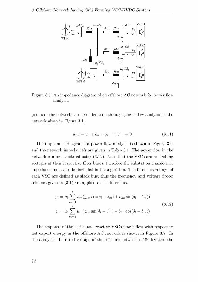
3 Offshore Network having Grid Forming VSC-HVDC System

VSC-1

VSC-2

VSC-3

u1 1

p1q1

u2 2

u3 3

u4 4 u5 5

u6 6

g15 jb15

jb1

jb45

g25 jb25

g36 jb36

jb2

jb3

p2q2

p3q3

p4q4

jb56

p6q6

WPP-1

WPP-2

Figure 3.6: An impedance diagram of an offshore AC network for power flowanalysis.

points of the network can be understood through power flow analysis on the

network given in Figure 3.1.

ur i = u0 + ku i · qi ∵ q0 i = 0 (3.11)

The impedance diagram for power flow analysis is shown in Figure 3.6,

and the network impedance’s are given in Table 3.1. The power flow in the

network can be calculated using (3.12). Note that the VSCs are controlling

voltages at their respective filter buses, therefore the substation transformer

impedance must also be included in the algorithm. The filter bus voltage of

each VSC are defined as slack bus, thus the frequency and voltage droop

schemes given in (3.1) are applied at the filter bus.

pl = ul

z∑m=1

um(glm cos(δl − δm) + blm sin(δl − δm))

ql = ul

z∑m=1

um(glm sin(δl − δm)− blm cos(δl − δm))

(3.12)

The response of the active and reactive VSCs power flow with respect to

net export energy in the offshore AC network is shown in Figure 3.7. In

the analysis, the rated voltage of the offshore network is 150 kV and the

72

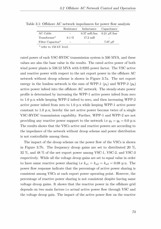
3.2 Offshore AC Network Control and Operation

Table 3.1: Offshore AC network impedances for power flow analysis

Resistance Inductance Capacitance

AC Cable - 0.37 mH/km 0.21 µF/km

Transformera 0.1 Ω 17.2 mH -

Filter Capacitora - - 7.07 µF

a refer to 150 kV level.

rated power of each VSC-HVDC transmission system is 500 MVA, and these

values are also the base value in the results. The rated active power of both

wind power plants is 538.52 MVA with 0.9285 power factor. The VSC active

and reactive power with respect to the net export power in the offshore AC

network without droop scheme is shown in Figure 3.7a. The net export

energy in the lossless network is the sum of WPP-1 (p4) and WPP-2 (p6)

active power infeed into the offshore AC network. The steady-state power

profile is determined by increasing the WPP-1 active power infeed from zero

to 1.0 p.u while keeping WPP-2 infeed to zero, and then increasing WPP-2

active power infeed from zero to 1.0 p.u while keeping WPP-1 active power

constant to 1.0 p.u, hereby the net active power become twice of a single

VSC-HVDC transmission capability. Further, WPP-1 and WPP-2 are not

providing any reactive power support to the network i.e q4 = q6 = 0.0 p.u.

The results shows that the VSCs active and reactive powers are according to

the impedance of the network without droop scheme and power distribution

is not controllable among them.

The impact of the droop scheme on the power flow of the VSCs is shown

in Figure 3.7b. The frequency droop gains are set to distributed 20 %,

32 %, and 48 % of the net export power among VSC-1, VSC-2, and VSC-3

respectively. While all the voltage droop gains are set to equal value in order

to have same reactive power sharing i.e ku1 = ku2 = ku3 = 0.08 p.u. The

power flow response indicate that the percentage of active power sharing is

consistent among VSCs at each export power operating point. However, the

percentage of reactive power sharing is not consistent despite having same

voltage droop gains. It shows that the reactive power in the offshore grid

depends on two main factors i.e actual active power flow through VSC and

the voltage droop gain. The impact of the active power flow on the reactive

73

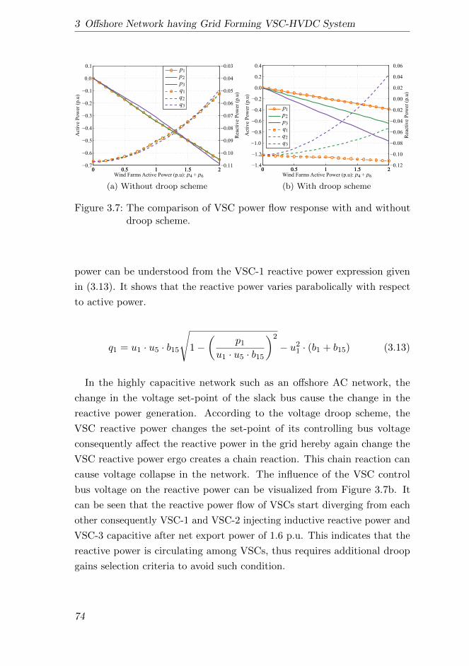
3 Offshore Network having Grid Forming VSC-HVDC System

0 0.5 1 1.5 20.7

0.6

0.5

0.4

0.3

0.2

0.1

0.0

0.1

Act

ive

Pow

er (

p.u

)

0 0.5 1 1.5 20.11

0.10

0.09

0.08

0.07

0.06

0.05

0.04

0.03

Rea

ctiv

e P

ow

er (

p.u

)

p1

p2

p3

q1

q2

q3

Wind Farms Active Power (p.u): p4 + p6

(a) Without droop scheme

0 0.5 1 1.5 21.4

1.2

1.0

0.8

0.6

0.4

0.2

0.0

0.2

0.4

Act

ive

Pow

er (

p.u

)

0 0.5 1 1.5 20.12

0.10

0.08

0.06

0.04

0.02

0.00

0.02

0.04

0.06

Rea

ctiv

e P

ow

er (

p.u

)

p1

p2

p3

q1

q2

q3

Wind Farms Active Power (p.u): p4 + p6

(b) With droop scheme

Figure 3.7: The comparison of VSC power flow response with and withoutdroop scheme.

power can be understood from the VSC-1 reactive power expression given

in (3.13). It shows that the reactive power varies parabolically with respect

to active power.

q1 = u1 · u5 · b15

√1−

(p1

u1 · u5 · b15

)2

− u21 · (b1 + b15) (3.13)

In the highly capacitive network such as an offshore AC network, the

change in the voltage set-point of the slack bus cause the change in the

reactive power generation. According to the voltage droop scheme, the

VSC reactive power changes the set-point of its controlling bus voltage

consequently affect the reactive power in the grid hereby again change the

VSC reactive power ergo creates a chain reaction. This chain reaction can

cause voltage collapse in the network. The influence of the VSC control

bus voltage on the reactive power can be visualized from Figure 3.7b. It

can be seen that the reactive power flow of VSCs start diverging from each

other consequently VSC-1 and VSC-2 injecting inductive reactive power and

VSC-3 capacitive after net export power of 1.6 p.u. This indicates that the

reactive power is circulating among VSCs, thus requires additional droop

gains selection criteria to avoid such condition.

74

3.2 Offshore AC Network Control and Operation

3.2.3 Method of Selecting Frequency and Voltage Droop Gains

The selection of frequency and voltage droop gains for the steady-state

operation depends on the operational requirement and the long term voltage

stability. The main operational requirement is the ability to control the

power distribution among the VSC-HVDC transmission systems which could

be an operator specification.

It is known that all VSCs active power flow direction would be same while

controlling the sharing of active power using droop gains. Thus, the active

power of VSC can be expressed as a factor α of the total power (ps) in the

offshore AC grid. The active power of each VSCs can be expressed as (3.14)

for n grid forming VSCs.

p1 = α1 · psp2 = α2 · ps

...

pn = αn · ps

(3.14)

Also, It is known that the total power must be equal to the sum of the

VSCs power, thus (3.14) can be simplified as (3.15).

ps = p1 + p2 + · · ·+ pn

ps =

(n∑i=1

αi

)ps

n∑i=1

αi = 1 ∀α ∈ < : 0 ≤ α ≤ 1

(3.15)

In order to satisfy condition given in (3.15), the nth VSC sharing factor

must be defined as (3.16).

αn = 1−n−1∑i=1

αi (3.16)

The condition of the nth VSC active power can be defined as (3.17) by

substituting (3.16) in (3.14).

75

3 Offshore Network having Grid Forming VSC-HVDC System

pn

(n−1∑i=1

αi

)−

(1−

n−1∑i=1

αi

)n−1∑i=1

pi = 0 (3.17)

For n − 1 VSCs, the distribution factor must be defined in order to

determine the droop values. This can be achieved by defining the relationship

between the distribution factor and the droop values by comparing (3.10)

with (3.14). Thus, the distribution factor of any ith VSC can be written as

(3.18).

αi =1

kf i· 1

n∑j=1

1

kf j

(3.18)

Similarly, consider β as the reactive power distribution factor then the

reactive power of each grid forming VSCs in the offshore AC network can

be expressed as (3.19).

q1 = β1 · qsq2 = β2 · qs

...

qn = βn · qs

(3.19)

Here, qs is the sum of the reactive power flowing through each grid forming

VSCs. Also, the reactive power sharing condition given in (3.20) must be

satisfied.

qs = q1 + q2 + · · ·+ qn =

n∑i=1

qi

n∑i=1

βi = 1 ∀β ∈ < : 0 ≤ β ≤ 1

(3.20)

Unlike frequency droop scheme, the relationship between reactive power

sharing factor (β) and the voltage droop gains (ku) cannot be explicitly

defined because of not having a common link between the VSCs control

busbars. However, the computation of voltage droop gains can be done with

76

3.2 Offshore AC Network Control and Operation

the common variable i.e reactive power. Thus, the condition for reactive

power sharing of ith VSCs can be defined as (3.21) for n grid forming VSCs

in the offshore AC network by substituting (3.20) into (3.19).

(1− βi) qi − βin∑j=1j 6=i

qj = 0 (3.21)

Note that n − 1 reactive power distribution factor (β) is required to

be defined in order to satisfy (3.20), also one system function would be

redundant if it is defined by (3.21) for all grid forming VSCs. Furthermore,

the busbars voltages are not considered in the selection of droop gains. As

explained in previous section that the reactive power flow of the VSCs

changes the controlling bus voltage level, and the difference between these

bus voltages may generate additional reactive power. The require reactive

power sharing can be achieved at high gain as well as at lower, however the

interaction between VSCs control busbars would be large at high voltage

droop gains. The impact of the voltage droop on the network can be

understood by analyzing the change it caused in the reactive power at the

load bus.

Consider that a load bus is directly connected with a VSC control bus.

The reactive power flow equation of the load bus given in (3.12) can be

expanded for the branches that are connected with the VSC control bus (i.e

filter bus) as (3.22).

ql − ulz−1∑m=1m 6=i

um glm sin(∆δlm)− blm cos(∆δlm)

−ului gli sin(∆δli)− bli cos(∆δli) = 0

(3.22)

Substitution of the voltage droop equation given in (3.11) into (3.22) yield

(3.23).

ql − ulz−1∑m=1m 6=i

umhlm − ulhli (u0 + ku iqi) = 0 (3.23)

77

3 Offshore Network having Grid Forming VSC-HVDC System

ql − ulz−1∑m=1m6=i

umhlm − ulu0hli

︸ ︷︷ ︸ku i=0

−ulku iqihli︸ ︷︷ ︸∆qk i

= 0 (3.24)

Here, z is the total number of AC busbars in the offshore AC network, i

is the VSC control busbar index, hlm = glm sin(∆δlm)− blm cos(∆δlm), and

hli = gli sin(∆δli)− bli cos(∆δli).

The first three terms in (3.24) are the reactive power mismatch without

voltage droop scheme at the load bus. The droop gain add the reactive

power (∆qk i) at the load bus as the function of VSC reactive power. In

case of one grid forming VSC in the network, this additional reactive power

largely impact on the network voltages since there are no sources available

other than cable capacitance to absorb it. The voltage droop scheme is not

required to be applied for single grid forming VSC in the offshore AC network.

However, the multiple grid forming VSCs in the offshore AC network can

exchange this additional reactive power (∆qk i) for balancing and to reduce

its impact on the network voltages. To achieve this, the criteria given in

(3.25) can be applied to determine the droop gains.

∆qk 1 + ∆qk 2 + · · ·+ ∆qk n = 0

n∑i=1

y∑l=1

ulku iqihli = 0 ∀i, l : i 6= l(3.25)

Here, y is the total number of busbars that is connected with ith VSCs

reference bus, n is the total number of grid forming VSCs in the offshore

AC network, ku i and qi are the voltage droop gain and reactive power of

ith VSC.

Steady-State Analysis: The optimum value of droop gains can be cal-

culated using above criteria to achieve desire power sharing among the

VSC-HVDC transmission system. To do so, an optimum power flow al-

gorithm is developed using (3.1), (3.10), (3.12), (3.17), (3.18), (3.21), and

(3.25) for the network shown in Figure 3.6. The solution is found using MAT-

78

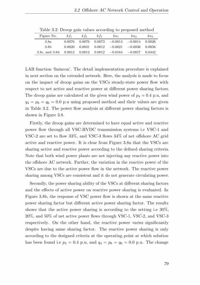
3.2 Offshore AC Network Control and Operation

Table 3.2: Droop gain values according to proposed method

Figure No. kf1 kf2 kf3 ku1 ku2 ku3

3.8a 0.0076 0.0076 0.0073 −0.0014 −0.0014 0.0026

3.8b 0.0020 0.0031 0.0012 −0.0021 −0.0036 0.0056

3.8c, and 3.8d 0.0012 0.0012 0.0012 −0.0164 −0.0857 0.0442

LAB function ‘fmincon’. The detail implementation procedure is explained

in next section on the extended network. Here, the analysis is made to focus

on the impact of droop gains on the VSCs steady-state power flow with

respect to net active and reactive power at different power sharing factors.

The droop gains are calculated at the given wind power of p4 = 0.4 p.u, and

q4 = p6 = q6 = 0.0 p.u using proposed method and their values are given

in Table 3.2. The power flow analysis at different power sharing factors is

shown in Figure 3.8.

Firstly, the droop gains are determined to have equal active and reactive

power flow through all VSC-HVDC transmission systems i.e VSC-1 and

VSC-2 are set to flow 33%, and VSC-3 flows 34% of net offshore AC grid

active and reactive power. It is clear from Figure 3.8a that the VSCs are

sharing active and reactive power according to the defined sharing criteria.

Note that both wind power plants are not injecting any reactive power into

the offshore AC network. Further, the variation in the reactive power of the

VSCs are due to the active power flow in the network. The reactive power

sharing among VSCs are consistent and it do not generate circulating power.

Secondly, the power sharing ability of the VSCs at different sharing factors

and the effects of active power on reactive power sharing is evaluated. In

Figure 3.8b, the response of VSC power flow is shown at the same reactive

power sharing factor but different active power sharing factor. The results

shows that the active power sharing is according to the setting i.e 30%,

20%, and 50% of net active power flows through VSC-1, VSC-2, and VSC-3

respectively. On the other hand, the reactive power varies significantly

despite having same sharing factor. The reactive power sharing is only

according to the designed criteria at the operating point at which solution

has been found i.e p4 = 0.4 p.u, and q4 = p6 = q6 = 0.0 p.u. The change

79

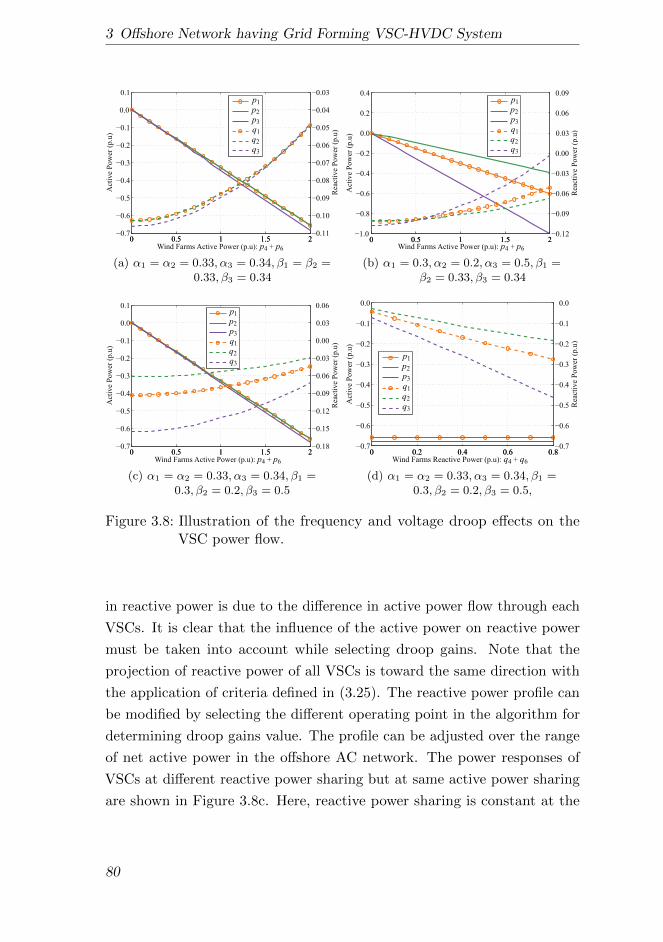
3 Offshore Network having Grid Forming VSC-HVDC System

0 0.5 1 1.5 20.7

0.6

0.5

0.4

0.3

0.2

0.1

0.0

0.1

Act

ive

Pow

er (

p.u

)

0 0.5 1 1.5 20.11

0.10

0.09

0.08

0.07

0.06

0.05

0.04

0.03

Rea

ctiv

e P

ow

er (

p.u

)

p1

p2

p3

q1

q2

q3

Wind Farms Active Power (p.u): p4 + p6

(a) α1 = α2 = 0.33, α3 = 0.34, β1 = β2 =0.33, β3 = 0.34

0 0.5 1 1.5 21.0

0.8

0.6

0.4

0.2

0.0

0.2

0.4

Act

ive

Pow

er (

p.u

)

0 0.5 1 1.5 20.12

0.09

0.06

0.03

0.00

0.03

0.06

0.09

Rea

ctiv

e P

ow

er (

p.u

)

p1

p2

p3

q1

q2

q3

Wind Farms Active Power (p.u): p4 + p6

(b) α1 = 0.3, α2 = 0.2, α3 = 0.5, β1 =β2 = 0.33, β3 = 0.34

0 0.5 1 1.5 20.7

0.6

0.5

0.4

0.3

0.2

0.1

0.0

0.1

Act

ive

Pow

er (

p.u

)

0 0.5 1 1.5 20.18

0.15

0.12

0.09

0.06

0.03

0.00

0.03

0.06

Rea

ctiv

e P

ow

er (

p.u

)

p1

p2

p3

q1

q2

q3

Wind Farms Active Power (p.u): p4 + p6

(c) α1 = α2 = 0.33, α3 = 0.34, β1 =0.3, β2 = 0.2, β3 = 0.5

0 0.2 0.4 0.6 0.80.7

0.6

0.5

0.4

0.3

0.2

0.1

0.0

Act

ive

Pow

er (

p.u

)

0 0.2 0.4 0.6 0.80.7

0.6

0.5

0.4

0.3

0.2

0.1

0.0

Rea

ctiv

e P

ow

er (

p.u

)

Wind Farms Reactive Power (p.u): q4 + q6

p1

p2

p3

q1

q2

q3

(d) α1 = α2 = 0.33, α3 = 0.34, β1 =0.3, β2 = 0.2, β3 = 0.5,

Figure 3.8: Illustration of the frequency and voltage droop effects on theVSC power flow.

in reactive power is due to the difference in active power flow through each

VSCs. It is clear that the influence of the active power on reactive power

must be taken into account while selecting droop gains. Note that the

projection of reactive power of all VSCs is toward the same direction with

the application of criteria defined in (3.25). The reactive power profile can

be modified by selecting the different operating point in the algorithm for

determining droop gains value. The profile can be adjusted over the range

of net active power in the offshore AC network. The power responses of

VSCs at different reactive power sharing but at same active power sharing

are shown in Figure 3.8c. Here, reactive power sharing is constant at the

80

3.2 Offshore AC Network Control and Operation

designed value throughout the variation of net active power in the offshore

AC grid. Yet again, the reactive power projection is same in all VSCs which

demonstrate that the unnecessary reactive power is not generated in the

network.

Thirdly, the analysis of VSCs power response is shown in Figure 3.8d

with respect to the net reactive power injection of wind power plants i.e

qs = q4 + q6. Both wind power plants are injecting maximum active power

i.e p4 = p6 = 1.0 p.u. In the analysis, the active power sharing is set to

equal. Here, the reactive power contributions are 30%, 20%, and 50% by

VSC-1, VSC-2, and VSC-3 respectively. The power flow profile is created by

first changing the power factor of WPP-1 from 1.0 to 0.9285 leading while

keeping WPP-1 power factor to 1.0, and then changing WPP-2 power factor

from 1.0 to 0.9285 leading. It is evident that the VSCs active power sharing

is according to the designed criteria at all operating points and it is not

influenced by the reactive power flow. Further, the reactive power sharing

is also consistent among the VSCs. Note that the generator oriented sign

convention is used in the results.

Time Domain Analysis: The proposed method of selecting frequency and

voltage droop gains is validated by performing nonlinear simulation of

the network shown in Figure 3.1. The frequency droop gains are set as

kf1 = 0.0020 p.u, kf2 = 0.0031 p.u, and kf3 = 0.0012 p.u. The voltage droop

gains setting are ku1 = −0.0021 p.u, ku2 = −0.0036 p.u, and ku3 = 0.0056 p.u.

The wind power plants reactive power set-points are q4 = q6 = 0.0 p.u. For

the dynamic analysis, the WPP-1 wind active power is changed from zero

to 1.0 p.u at 2.0 s, and the WPP-2 active power is changed from zero to

1.0 p.u at 4.0 s. The power and frequency responses of the VSCs are shown

in Figure 3.9.

During first step change in power, the VSC-1 is exporting 0.3 p.u active

power to onshore whereas VSC-2 and VSC-3 are exporting 0.2 p.u and

0.5 p.u respectively. At the full power infeed by both wind power plants,

the VSC-1 reaches its active power export limit. According to the network

parameters, the maximum active power sharing factor (αi) that can be

assigned to any VSCs is 0.5 at maximum wind energy infeed. The wind

81

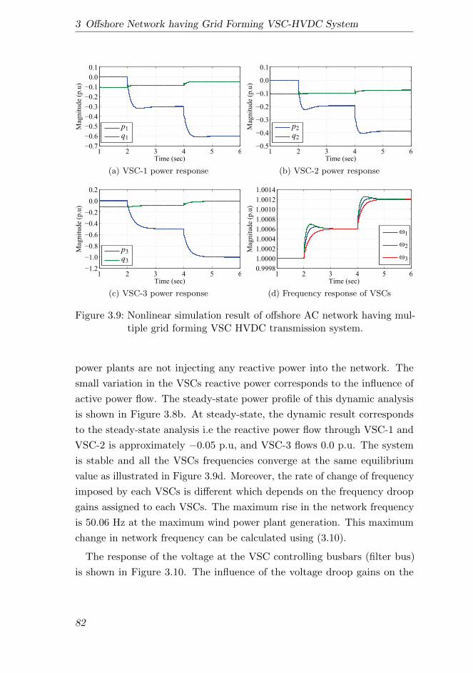
3 Offshore Network having Grid Forming VSC-HVDC System

1 2 3 4 5 60.7

0.6

0.5

0.4

0.3

0.2

0.1

0.0

0.1

Time (sec)

Mag

nit

ude

(p.u

)

p1

q1

(a) VSC-1 power response

1 2 3 4 5 60.5

0.4

0.3

0.2

0.1

0.0

0.1

Time (sec)

Mag

nit

ude

(p.u

)

p2

q2

(b) VSC-2 power response

1 2 3 4 5 61.2

1.0

0.8

0.6

0.4

0.2

0.0

0.2

Time (sec)

Mag

nit

ude

(p.u

)

p3

q3

(c) VSC-3 power response

1 2 3 4 5 60.9998

1.0000

1.0002

1.0004

1.0006

1.0008

1.0010

1.0012

1.0014

Time (sec)

Mag

nit

ude

(p.u

)

1

2

3

(d) Frequency response of VSCs

Figure 3.9: Nonlinear simulation result of offshore AC network having mul-tiple grid forming VSC HVDC transmission system.

power plants are not injecting any reactive power into the network. The

small variation in the VSCs reactive power corresponds to the influence of

active power flow. The steady-state power profile of this dynamic analysis

is shown in Figure 3.8b. At steady-state, the dynamic result corresponds

to the steady-state analysis i.e the reactive power flow through VSC-1 and

VSC-2 is approximately −0.05 p.u, and VSC-3 flows 0.0 p.u. The system

is stable and all the VSCs frequencies converge at the same equilibrium

value as illustrated in Figure 3.9d. Moreover, the rate of change of frequency

imposed by each VSCs is different which depends on the frequency droop

gains assigned to each VSCs. The maximum rise in the network frequency

is 50.06 Hz at the maximum wind power plant generation. This maximum

change in network frequency can be calculated using (3.10).

The response of the voltage at the VSC controlling busbars (filter bus)

is shown in Figure 3.10. The influence of the voltage droop gains on the

82

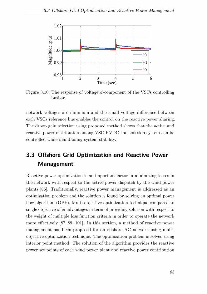
3.3 Offshore Grid Optimization and Reactive Power Management

1 2 3 4 5 60.98

0.99

1.00

1.01

1.02

Time (sec)

Mag

nit

ude

(p.u

)u1

u2

u3

Figure 3.10: The response of voltage d -component of the VSCs controllingbusbars.

network voltages are minimum and the small voltage difference between

each VSCs reference bus enables the control on the reactive power sharing.

The droop gain selection using proposed method shows that the active and

reactive power distribution among VSC-HVDC transmission system can be

controlled while maintaining system stability.

3.3 Offshore Grid Optimization and Reactive Power

Management

Reactive power optimization is an important factor in minimizing losses in

the network with respect to the active power dispatch by the wind power

plants [86]. Traditionally, reactive power management is addressed as an

optimization problem and the solution is found by solving an optimal power

flow algorithm (OPF). Multi-objective optimization technique compared to

single objective offer advantages in term of providing solution with respect to

the weight of multiple loss function criteria in order to operate the network

more effectively [87–89, 101]. In this section, a method of reactive power

management has been proposed for an offshore AC network using multi-

objective optimization technique. The optimization problem is solved using

interior point method. The solution of the algorithm provides the reactive

power set points of each wind power plant and reactive power contribution

83

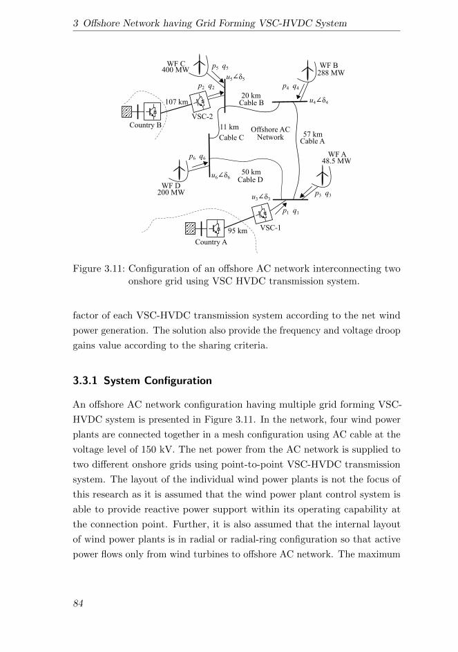
3 Offshore Network having Grid Forming VSC-HVDC System

Offshore ACNetwork

Country B

u5 5

WF C400 MW

WF B288 MW

WF A48.5 MW

WF D200 MW

Cable A57 km

Cable B20 km

Cable C

11 km

VSC-2

Country A

VSC-1

p5 q5

Cable D50 km

p4 q4

p3 q3

95 km

107 km

p6 q6

p2 q2

p1 q1

u4 4

u3 3

u6 6

Figure 3.11: Configuration of an offshore AC network interconnecting twoonshore grid using VSC HVDC transmission system.

factor of each VSC-HVDC transmission system according to the net wind

power generation. The solution also provide the frequency and voltage droop

gains value according to the sharing criteria.

3.3.1 System Configuration

An offshore AC network configuration having multiple grid forming VSC-

HVDC system is presented in Figure 3.11. In the network, four wind power

plants are connected together in a mesh configuration using AC cable at the

voltage level of 150 kV. The net power from the AC network is supplied to

two different onshore grids using point-to-point VSC-HVDC transmission

system. The layout of the individual wind power plants is not the focus of

this research as it is assumed that the wind power plant control system is

able to provide reactive power support within its operating capability at

the connection point. Further, it is also assumed that the internal layout

of wind power plants is in radial or radial-ring configuration so that active

power flows only from wind turbines to offshore AC network. The maximum

84

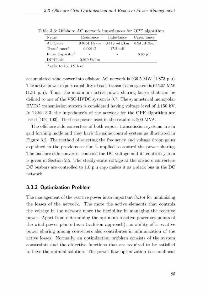
3.3 Offshore Grid Optimization and Reactive Power Management

Table 3.3: Offshore AC network impedances for OPF algorithm

Name Resistance Inductance Capacitance

AC Cable 0.0151 Ω/km 0.118 mH/km 0.24 µF/km

Transformera 0.099 Ω 17.2 mH -

Filter Capacitora - - 6.85 µF

DC Cable 0.019 Ω/km - -

a refer to 150 kV level.

accumulated wind power into offshore AC network is 936.5 MW (1.873 p.u).

The active power export capability of each transmission system is 655.55 MW

(1.31 p.u). Thus, the maximum active power sharing factor that can be

defined to one of the VSC-HVDC system is 0.7. The symmetrical monopolar

HVDC transmission system is considered having voltage level of ±150 kV.

In Table 3.3, the impedance’s of the network for the OPF algorithm are

listed [102, 103]. The base power used in the results is 500 MVA.

The offshore side converters of both export transmission systems are in

grid forming mode and they have the same control system as illustrated in

Figure 3.2. The method of selecting the frequency and voltage droop gains

explained in the previous section is applied to control the power sharing.

The onshore side converter controls the DC voltage and its control system

is given in Section 2.5. The steady-state voltage at the onshore converters

DC busbars are controlled to 1.0 p.u ergo makes it as a slack bus in the DC

network.

3.3.2 Optimization Problem

The management of the reactive power is an important factor for minimizing

the losses of the network. The more the active elements that controls

the voltage in the network more the flexibility in managing the reactive

power. Apart from determining the optimum reactive power set-points of

the wind power plants (as a tradition approach), an ability of a reactive

power sharing among converters also contributes in minimization of the

active losses. Normally, an optimization problem consists of the system

constraints and the objective functions that are required to be satisfied

to have the optimal solution. The power flow optimization is a nonlinear

85

3 Offshore Network having Grid Forming VSC-HVDC System

non-convex problem and it has large number of local minima. A local

minima can be designated as a global minima within the closed interval

define by the constraints and boundaries. The system constraints and limits

ensure that the same local minima is found at different initial values for the

given predefined conditions and sets of inputs or get no solution at all. An

optimization algorithm based on interior-point method is well suited to find

the solution of nonlinear system. For the analysis, the optimization problem

has been implemented using sets of nonlinear equations that are derived as

follows:

Constraints: The network configuration and the control conditions are defi-

ned as a nonlinear equalities and inequalities constraints for the formulation

of an optimization problem. In general, these constraints can be expressed

as (3.26).

System

g(x) ≤ 0

h(x) = 0(3.26)

According to the problem, these constraints consists of AC and DC

network topologies, VSCs droop control equations, power sharing criteria,

and optimization variables boundary limit.

a) Offshore AC and DC Network Topology : The network topology is an

equality constraint and it is usually defined by the power flow equation.

The power flow equations for the AC network are defined using (3.12).

In the DC network only the active power exists which can be defined

for the OPF algorithm as (3.27).

Pi = Ui

k∑j=1

UjGij (3.27)

The link between the AC and DC power flow is established by defining

active power loss function as (3.28).

pvsc + Pdc + Ploss = 0 (3.28)

86

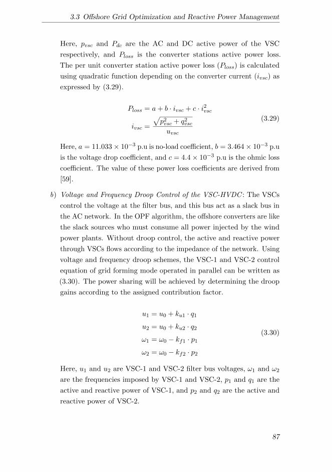
3.3 Offshore Grid Optimization and Reactive Power Management

Here, pvsc and Pdc are the AC and DC active power of the VSC

respectively, and Ploss is the converter stations active power loss.

The per unit converter station active power loss (Ploss) is calculated

using quadratic function depending on the converter current (ivsc) as

expressed by (3.29).

Ploss = a+ b · ivsc + c · i2vsc

ivsc =

√p2vsc + q2

vsc

uvsc

(3.29)

Here, a = 11.033× 10−3 p.u is no-load coefficient, b = 3.464× 10−3 p.u

is the voltage drop coefficient, and c = 4.4× 10−3 p.u is the ohmic loss

coefficient. The value of these power loss coefficients are derived from

[59].

b) Voltage and Frequency Droop Control of the VSC-HVDC : The VSCs

control the voltage at the filter bus, and this bus act as a slack bus in

the AC network. In the OPF algorithm, the offshore converters are like

the slack sources who must consume all power injected by the wind

power plants. Without droop control, the active and reactive power

through VSCs flows according to the impedance of the network. Using

voltage and frequency droop schemes, the VSC-1 and VSC-2 control

equation of grid forming mode operated in parallel can be written as

(3.30). The power sharing will be achieved by determining the droop

gains according to the assigned contribution factor.

u1 = u0 + ku1 · q1

u2 = u0 + ku2 · q2

ω1 = ω0 − kf1 · p1

ω2 = ω0 − kf2 · p2

(3.30)

Here, u1 and u2 are VSC-1 and VSC-2 filter bus voltages, ω1 and ω2

are the frequencies imposed by VSC-1 and VSC-2, p1 and q1 are the

active and reactive power of VSC-1, and p2 and q2 are the active and

reactive power of VSC-2.

87

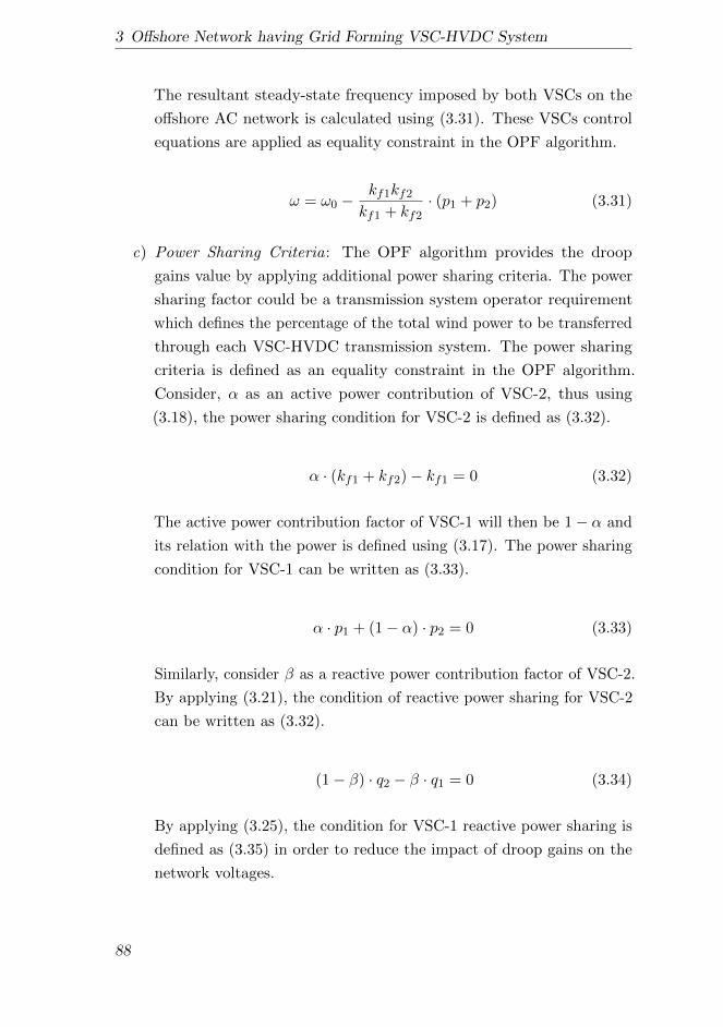
3 Offshore Network having Grid Forming VSC-HVDC System

The resultant steady-state frequency imposed by both VSCs on the

offshore AC network is calculated using (3.31). These VSCs control

equations are applied as equality constraint in the OPF algorithm.

ω = ω0 −kf1kf2

kf1 + kf2· (p1 + p2) (3.31)

c) Power Sharing Criteria: The OPF algorithm provides the droop

gains value by applying additional power sharing criteria. The power

sharing factor could be a transmission system operator requirement

which defines the percentage of the total wind power to be transferred

through each VSC-HVDC transmission system. The power sharing

criteria is defined as an equality constraint in the OPF algorithm.

Consider, α as an active power contribution of VSC-2, thus using

(3.18), the power sharing condition for VSC-2 is defined as (3.32).

α · (kf1 + kf2)− kf1 = 0 (3.32)

The active power contribution factor of VSC-1 will then be 1− α and

its relation with the power is defined using (3.17). The power sharing

condition for VSC-1 can be written as (3.33).

α · p1 + (1− α) · p2 = 0 (3.33)

Similarly, consider β as a reactive power contribution factor of VSC-2.

By applying (3.21), the condition of reactive power sharing for VSC-2

can be written as (3.32).

(1− β) · q2 − β · q1 = 0 (3.34)

By applying (3.25), the condition for VSC-1 reactive power sharing is

defined as (3.35) in order to reduce the impact of droop gains on the

network voltages.

88

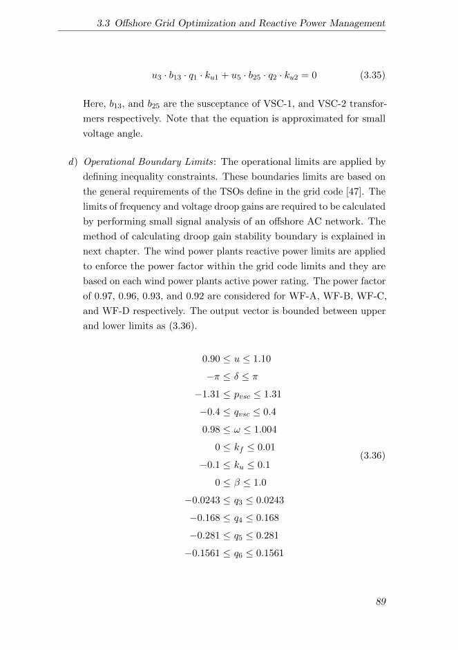
3.3 Offshore Grid Optimization and Reactive Power Management

u3 · b13 · q1 · ku1 + u5 · b25 · q2 · ku2 = 0 (3.35)

Here, b13, and b25 are the susceptance of VSC-1, and VSC-2 transfor-

mers respectively. Note that the equation is approximated for small

voltage angle.

d) Operational Boundary Limits: The operational limits are applied by

defining inequality constraints. These boundaries limits are based on

the general requirements of the TSOs define in the grid code [47]. The

limits of frequency and voltage droop gains are required to be calculated

by performing small signal analysis of an offshore AC network. The

method of calculating droop gain stability boundary is explained in

next chapter. The wind power plants reactive power limits are applied

to enforce the power factor within the grid code limits and they are

based on each wind power plants active power rating. The power factor

of 0.97, 0.96, 0.93, and 0.92 are considered for WF-A, WF-B, WF-C,

and WF-D respectively. The output vector is bounded between upper

and lower limits as (3.36).

0.90 ≤ u ≤ 1.10

−π ≤ δ ≤ π

−1.31 ≤ pvsc ≤ 1.31

−0.4 ≤ qvsc ≤ 0.4

0.98 ≤ ω ≤ 1.004

0 ≤ kf ≤ 0.01

−0.1 ≤ ku ≤ 0.1

0 ≤ β ≤ 1.0

−0.0243 ≤ q3 ≤ 0.0243

−0.168 ≤ q4 ≤ 0.168

−0.281 ≤ q5 ≤ 0.281

−0.1561 ≤ q6 ≤ 0.1561

(3.36)

89

3 Offshore Network having Grid Forming VSC-HVDC System

In addition, the maximum frequency deviation limit is imposed by

applying condition given in (3.10) at maximum power. It is a nonlinear

inequality constraint defined as (3.37).

pmax · kf1 · kf2 −∆ωmax (kf1 + kf2) < 0 (3.37)

Objective Functions: The objective function defines the criteria of finding

the best solution from all feasible solution for an optimization problem.

Multiple objective functions can also be applied for optimal solution. Ho-

wever, simultaneously optimizing each objective functions may not lead to

a single solution for nontrivial multi-objective optimization problem. In

that case, objective functions are said to be conflicting and the solution

of the system cannot be found without degrading the objective values. A

tradeoff is required between the functions in order to obtain a favorable

solution. The simplest approach to achieve the trade-off among the objective

functions is a weighted sum method [104]. In weighted sum method, a

single function is formulated by multiplying each objective function with

a predefined weighting factor as expressed by (3.38). The weighting factor

defines the relative magnitude of each function in the overall solution. Pareto

Front analysis of the objective functions can then be applied to choose the

optimal operating points and the best solution.

min F (x)

F (x) =

h∑m=1

γmfm (x) γm ∈ [0, 1](3.38)

Here, γm is the weight of the mth objective function. In general, the

weights are selected to satisfy (3.39).(h∑

m=1

γm

)= 1 (3.39)

An objective function can either be a loss function or profit function but all

objectives must be converted into one type for weighted sum method. Two

objective functions are selected for the optimization problem as expressed

90

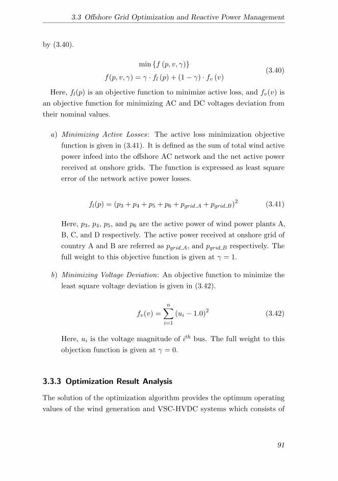
3.3 Offshore Grid Optimization and Reactive Power Management

by (3.40).

min f (p, v, γ)

f(p, v, γ) = γ · fl (p) + (1− γ) · fv (v)(3.40)

Here, fl(p) is an objective function to minimize active loss, and fv(v) is

an objective function for minimizing AC and DC voltages deviation from

their nominal values.

a) Minimizing Active Losses: The active loss minimization objective

function is given in (3.41). It is defined as the sum of total wind active

power infeed into the offshore AC network and the net active power

received at onshore grids. The function is expressed as least square

error of the network active power losses.

fl(p) = (p3 + p4 + p5 + p6 + pgrid A + pgrid B)2 (3.41)

Here, p3, p4, p5, and p6 are the active power of wind power plants A,

B, C, and D respectively. The active power received at onshore grid of

country A and B are referred as pgrid A, and pgrid B respectively. The

full weight to this objective function is given at γ = 1.

b) Minimizing Voltage Deviation: An objective function to minimize the

least square voltage deviation is given in (3.42).

fv(v) =

n∑i=1

(ui − 1.0)2 (3.42)

Here, ui is the voltage magnitude of ith bus. The full weight to this

objection function is given at γ = 0.

3.3.3 Optimization Result Analysis

The solution of the optimization algorithm provides the optimum operating

values of the wind generation and VSC-HVDC systems which consists of

91

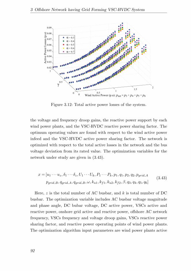
3 Offshore Network having Grid Forming VSC-HVDC System

00.5

11.5

2

0

0.5

1

0.02

0.03

0.04

0.05

0.06

0.07

0.08

0.09

Wind Active Power (p.u): pnet = p3 + p4 + p5 + p6

Act

ive

Pow

er L

oss

es (

p.u

)

= 0.3

= 0.4

= 0.5

= 0.6

= 0.7

Figure 3.12: Total active power losses of the system.

the voltage and frequency droop gains, the reactive power support by each

wind power plants, and the VSC-HVDC reactive power sharing factor. The

optimum operating values are found with respect to the wind active power

infeed and the VSC-HVDC active power sharing factor. The network is

optimized with respect to the total active losses in the network and the bus

voltage deviation from its rated value. The optimization variables for the

network under study are given in (3.43).

x = [u1 · · ·uz, δ1 · · · δz, U1 · · ·Uk, P1 · · ·Pk, p1, q1, p2, q2, pgrid A

pgrid B, qgrid A, qgrid B, ω, ku1, kf1, ku2, kf2, β, q3, q4, q5, q6](3.43)

Here, z is the total number of AC busbar, and k is total number of DC

busbar. The optimization variable includes AC busbar voltage magnitude

and phase angle, DC bubar voltage, DC active power, VSCs active and

reactive power, onshore grid active and reactive power, offshore AC network

frequency, VSCs frequency and voltage droop gains, VSCs reactive power

sharing factor, and reactive power operating points of wind power plants.

The optimization algorithm input parameters are wind power plants active

92

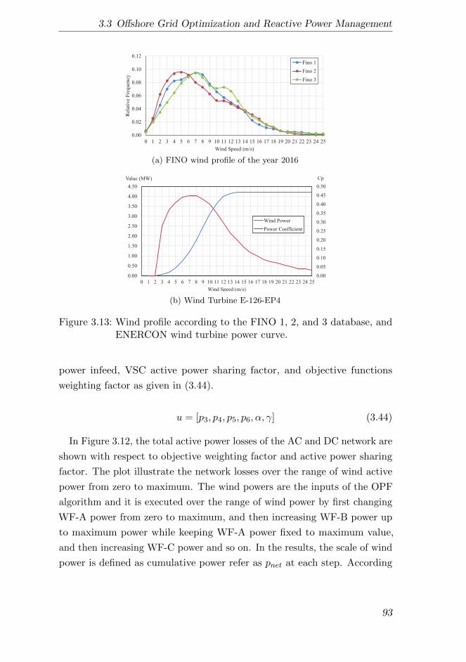
3.3 Offshore Grid Optimization and Reactive Power Management

0.00

0.02

0.04

0.06

0.08

0.10

0.12

0 1 2 3 4 5 6 7 8 9 10 11 12 13 14 15 16 17 18 19 20 21 22 23 24 25

Rel

ativ

e F

req

uen

cy

Wind Speed (m/s)

Fino 1

Fino 2

Fino 3

(a) FINO wind profile of the year 2016

0.00

0.05

0.10

0.15

0.20

0.25

0.30

0.35

0.40

0.45

0.50

0.00

0.50

1.00

1.50

2.00

2.50

3.00

3.50

4.00

4.50

0 1 2 3 4 5 6 7 8 9 10 11 12 13 14 15 16 17 18 19 20 21 22 23 24 25

CpValue (MW)

Wind Speed (m/s)

Wind Power

Power Coefficient

(b) Wind Turbine E-126-EP4

Figure 3.13: Wind profile according to the FINO 1, 2, and 3 database, andENERCON wind turbine power curve.

power infeed, VSC active power sharing factor, and objective functions

weighting factor as given in (3.44).

u = [p3, p4, p5, p6, α, γ] (3.44)

In Figure 3.12, the total active power losses of the AC and DC network are

shown with respect to objective weighting factor and active power sharing

factor. The plot illustrate the network losses over the range of wind active

power from zero to maximum. The wind powers are the inputs of the OPF

algorithm and it is executed over the range of wind power by first changing

WF-A power from zero to maximum, and then increasing WF-B power up

to maximum power while keeping WF-A power fixed to maximum value,

and then increasing WF-C power and so on. In the results, the scale of wind

power is defined as cumulative power refer as pnet at each step. According

93

3 Offshore Network having Grid Forming VSC-HVDC System

1.0302 1.0303 1.0304 1.0305 1.0306 1.0307 1.0308

x 103

2.28

2.31

2.34

2.37

2.40

2.43

2.46x 10

4

0 0.2 0.4 0.6 0.8 1

fv(v)

fl(p)

(a) Pareto Front at α = 0.5, andpnet = 0.688 p.u

6.210 6.215 6.220 6.225 6.230 6.235

x 103

0.7

0.8

0.9

1.0

1.1

1.2

1.3

1.4x 10

3

0 0.2 0.4 0.6 0.8 1

fv(v)

(b) Pareto Front at α = 0.5, andpnet = 1.8753 p.u

Figure 3.14: Pareto Front analysis of objective functions with respect toobjective weighting factor (γ).

to the result, the active power loss variation is relatively low with respect to

the objective function weighting factor. The variation of active power loss

with respect to the power sharing factor can be observed at high wind infeed

i.e the minimum losses in the network are at α = 0.5. Large wind power is

installed near country B therefore the network produces high active power

losses at α = 0.3.

The average power infeed by the wind power plants into the offshore AC

network is calculated using wind profile of FINO database [105]. FINO is a

research project started in 2002 having funding support by Federal Ministry

for the Environment, Nature, Conservation, Building and Nuclear Safety

(BMU) of Germany. The database provide meteorological and oceanographic

measurement made at three research platforms in the North and Baltic Seas.

The wind profile of FINO 1, 2 and 3 are shown in Figure 3.13a over the

period of one year. By considering FINO 1 wind profile for WF-C and WF-D,

the average wind speed of 8 m/s is considered for both wind power plants.

FINO 2 wind profile is considered for WF-A which give the wind speed of

5 m/s. And, the wind speed of 7 m/s is assumed for WF-B by considering

FINO 3 wind profile. By considering the power curve of ENERCON wind

turbine E-126-EP4 given in Figure 3.13b for all wind power plants, the most

94

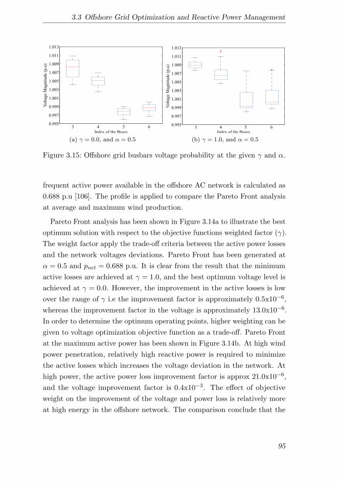
3.3 Offshore Grid Optimization and Reactive Power Management

0.995

0.997

0.999

1.001

1.003

1.005

1.007

1.009

1.011

1.013

3

Index of the Buses

Vo

ltag

e M

agn

itu

de

(p.u

)

4 5 6

(a) γ = 0.0, and α = 0.5

0.995

0.997

0.999

1.001

1.003

1.005

1.007

1.009

1.011

1.013

3Index of the Buses

Vo

ltag

e M

agn

itu

de

(p.u

)

4 5 6

(b) γ = 1.0, and α = 0.5

Figure 3.15: Offshore grid busbars voltage probability at the given γ and α.

frequent active power available in the offshore AC network is calculated as

0.688 p.u [106]. The profile is applied to compare the Pareto Front analysis

at average and maximum wind production.

Pareto Front analysis has been shown in Figure 3.14a to illustrate the best

optimum solution with respect to the objective functions weighted factor (γ).

The weight factor apply the trade-off criteria between the active power losses

and the network voltages deviations. Pareto Front has been generated at

α = 0.5 and pnet = 0.688 p.u. It is clear from the result that the minimum

active losses are achieved at γ = 1.0, and the best optimum voltage level is

achieved at γ = 0.0. However, the improvement in the active losses is low

over the range of γ i.e the improvement factor is approximately 0.5x10−6,

whereas the improvement factor in the voltage is approximately 13.0x10−6.

In order to determine the optimum operating points, higher weighting can be

given to voltage optimization objective function as a trade-off. Pareto Front

at the maximum active power has been shown in Figure 3.14b. At high wind

power penetration, relatively high reactive power is required to minimize

the active losses which increases the voltage deviation in the network. At

high power, the active power loss improvement factor is approx 21.0x10−6,

and the voltage improvement factor is 0.4x10−3. The effect of objective

weight on the improvement of the voltage and power loss is relatively more

at high energy in the offshore network. The comparison conclude that the

95

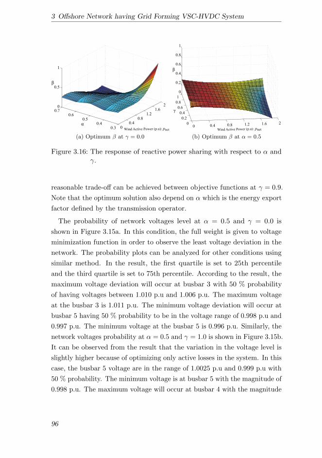
3 Offshore Network having Grid Forming VSC-HVDC System

00.4

0.81.2

1.62

0.30.4

0.50.6

0.70

0.5

1

Wind Active Power (p.u): pnet

(a) Optimum β at γ = 0.0

0 0.4 0.8 1.2 1.6 20

0.2

0.4

0.6

0.8

1

0

0.2

0.4

0.6

0.8

1

Wind Active Power (p.u): pnet

(b) Optimum β at α = 0.5

Figure 3.16: The response of reactive power sharing with respect to α andγ.

reasonable trade-off can be achieved between objective functions at γ = 0.9.

Note that the optimum solution also depend on α which is the energy export

factor defined by the transmission operator.

The probability of network voltages level at α = 0.5 and γ = 0.0 is

shown in Figure 3.15a. In this condition, the full weight is given to voltage

minimization function in order to observe the least voltage deviation in the

network. The probability plots can be analyzed for other conditions using

similar method. In the result, the first quartile is set to 25th percentile

and the third quartile is set to 75th percentile. According to the result, the

maximum voltage deviation will occur at busbar 3 with 50 % probability

of having voltages between 1.010 p.u and 1.006 p.u. The maximum voltage

at the busbar 3 is 1.011 p.u. The minimum voltage deviation will occur at

busbar 5 having 50 % probability to be in the voltage range of 0.998 p.u and

0.997 p.u. The minimum voltage at the busbar 5 is 0.996 p.u. Similarly, the

network voltages probability at α = 0.5 and γ = 1.0 is shown in Figure 3.15b.

It can be observed from the result that the variation in the voltage level is

slightly higher because of optimizing only active losses in the system. In this

case, the busbar 5 voltage are in the range of 1.0025 p.u and 0.999 p.u with

50 % probability. The minimum voltage is at busbar 5 with the magnitude of

0.998 p.u. The maximum voltage will occur at busbar 4 with the magnitude

96

3.3 Offshore Grid Optimization and Reactive Power Management

0.0 0.5 1.0 1.5 2.00.02

0.03

0.04

0.05

0.06

0.07

0.08

0.09A

ctiv

e P

ow

er L

oss

(p.u

)

Without Voltage Droop

Voltage Droop: =0.5

Wind Active Power(p.u): pnet

(a)

0.0 0.5 1.0 1.5 2.00.999

1.000

1.001

1.002

1.003

1.004

1.005

Fre

quen

cy (

p.u

)

Network

VSC 1 (Interpolated)

VSC 2 (Interpolated)

Wind Active Power (p.u): pnet

(b)

Figure 3.17: The responses of active power loss comparison with and withoutvoltage droop control, and the frequencies at α = 0.3 andγ = 1.0.

of 1.012 p.u. The results show that the voltages are within the required

operating range.

To achieve the minimum loss, the reactive power sharing (β) between

converters must also be optimally chosen. The response of β with respect to

the wind power infeed and α is shown in Figure 3.16a. Here, the weighting

factor is assigned to γ = 0.0. It is clear that more reactive power contribution

is required by the VSC-2 when the large power is transferred to the country

A at high wind penetration. Furthermore, the VSC-2 need to have more

reactive power compared to VSC-1 for α < 0.5 and almost all of the reactive

power must be provided by VSC-1 at α = 0.7, when the net wind power is

greater than 1.0 p.u. On the other hand, the reactive power sharing factor

is approximately 0.3 up to 1.0 p.u net wind power.

The influence of the weighting factor can be observed on the β from

Figure 3.16b for α = 0.5. It can be seen that β is relatively constant with

respect of γ and changes mainly with respect of wind power. As the affect

of γ is significant on the minimization of two objective functions at high

power. It can be seen that more contribution is required from the VSC-1 at

high wind power in order to minimize the voltage deviation.

The comparison of the active power losses with and without voltage droop

97

3 Offshore Network having Grid Forming VSC-HVDC System

0.0 0.5 1.0 1.5 2.00.03

0.02

0.01

0.00

0.01

WP

PA

Rea

ctiv

e P

ow

er (

p.u

)Without Voltage Droop

Voltage Droop: = 0.5

Wind Active Power (p.u): pnet

(a)

0.0 0.5 1.0 1.5 2.00.18

0.15

0.12

0.09

0.06

0.03

0.00

0.03

WP

PB

Rea

ctiv

e P

ow

er (

p.u

)

Without Voltage Droop

Voltage Droop: = 0.5

(b)

0.0 0.5 1.0 1.5 2.00.30

0.25

0.20

0.15

0.10

0.05

0.00

0.05

WP

PC

Rea

ctiv

e P

ow

er (

p.u

)

Without Voltage Droop

Voltage Droop: = 0.5

(c)

0.0 0.5 1.0 1.5 2.00.16

0.12

0.08

0.04

0.00

0.04

WP

PD

Rea

ctiv

e P

ow

er (

p.u

)

Without Voltage Droop

Voltage Droop: = 0.5

Wind Active Power (p.u): pnet

(d)

Figure 3.18: Comparison of the reactive power support by wind power plantsat α = 0.3, and γ = 1.0 with and without voltage droop control.

schemes is shown in Figure 3.17a. No voltage droop scheme means that both

offshore converters of HVDC transmission system are controlling the bus

voltages at the fixed set-points i.e 1.0 p.u. In this case, the reactive power

flow depends on the network impedance and converter active power. Thus,

it is not possible to control the contribution of each VSCs reactive power.

The response shows that the active power loss is same in both cases however

the application of the voltage droop provides additional degree to control

the reactive power sharing of the VSCs. The transmission operator can

additionally optimize the cost with the control over reactive power sharing.

The steady-state frequencies respons are shown in Figure 3.17b. It is clear

98

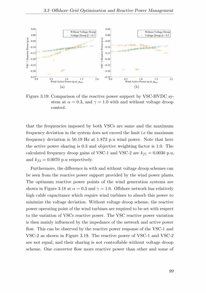
3.3 Offshore Grid Optimization and Reactive Power Management

0.0 0.5 1.0 1.5 2.00.35

0.30

0.25

0.20

0.15

0.10

0.05

0.00

0.05V

SC

1 R

eact

ive

Pow

er (

p.u

)

Without Voltage Droop

Voltage Droop: = 0.5

Wind Active Power (p.u): pnet

(a)

0.0 0.5 1.0 1.5 2.00.35

0.30

0.25

0.20

0.15

0.10

0.05

0.00

0.05

VS

C2 R

eact

ive

Pow

er (

p.u

)

Without Voltage Droop

Voltage Droop: = 0.5

Wind Active Power (p.u): pnet

(b)

Figure 3.19: Comparison of the reactive power support by VSC-HVDC sy-stem at α = 0.3, and γ = 1.0 with and without voltage droopcontrol.

that the frequencies imposed by both VSCs are same and the maximum

frequency deviation in the system does not exceed the limit i.e the maximum

frequency deviation is 50.19 Hz at 1.873 p.u wind power. Note that here

the active power sharing is 0.3 and objective weighting factor is 1.0. The

calculated frequency droop gains of VSC-1 and VSC-2 are kf1 = 0.0030 p.u,

and kf2 = 0.0070 p.u respectively.

Furthermore, the difference in with and without voltage droop schemes can

be seen from the reactive power support provided by the wind power plants.

The optimum reactive power points of the wind generation systems are

shown in Figure 3.18 at α = 0.3 and γ = 1.0. Offshore network has relatively

high cable capacitance which require wind turbines to absorb this power to

minimize the voltage deviation. Without voltage droop scheme, the reactive

power operating point of the wind turbines are required to be set with respect

to the variation of VSCs reactive power. The VSC reactive power variation

is then mainly influenced by the impedance of the network and active power

flow. This can be observed by the reactive power response of the VSC-1 and

VSC-2 as shown in Figure 3.19. The reactive power of VSC-1 and VSC-2

are not equal, and their sharing is not controllable without voltage droop

scheme. One converter flow more reactive power than other and some of

99

3 Offshore Network having Grid Forming VSC-HVDC System

the reactive power operating points are near to their limits, consequently

reactive power operating point of wind power plants are influenced. On the

other hand, reactive power flow is consistent and equally shared by both

VSC-HVDC transmission systems using voltage droop scheme. The voltage

droop scheme provides better control of reactive power in the offshore AC

network, and they are well within the limits. The desire reactive power

contribution by each VSCs can be assigned by setting voltage and frequency

droop gains value acquire through optimization algorithm. For the studied

system, the voltage droop gains at α = 0.3, β = 0.5, and γ = 1.0 are found

as ku1 = −0.0446 p.u, and ku2 = 0.0451 p.u.

3.4 Summary

Large offshore wind power plants installed at North Sea will make future

European energy efficient and affordable. The concept of offshore AC

network enables the integration of such high wind energy generations with

the onshore grids. In this chapter, the control scheme of grid forming voltage

source converters is proposed for an offshore AC network that has multiple

VSC-HVDC transmission systems. Frequency and voltage droop schemes

are proposed to share active and reactive power among transmission systems.

Later, a method to select these gains according to operational requirement

is presented. The proposed method is analyzed both for steady-state and

dynamic performance. It is concluded that the frequency and voltage droops

are interlinked and required to be designed by considering both active and

reactive power flows. Furthermore, it has been demonstrated that the VSCs

can control the power flow using droop scheme which provides additional

degree of freedom to manage power losses in the network. In the end, an

optimization problem has been addressed to demonstrate the ability of

VSCs to manage reactive power in the offshore AC network. An offshore

AC network can be utilized as a mediator between two different countries

electrical transmission systems hereby enables the trade. In comparison to

an alternative MTDC HVDC transmission system topology, net active power

in the offshore AC network can be higher than a single HVDC transmission

system. In addition, it does not require DC circuit breaker and protection

100

3.4 Summary

can be done through conventional AC protection scheme. However, the

addition of the droop scheme influences the network stability which is studied

in the next chapter.

101

102

4 Dynamic and Stability Analysis of

an Offshore AC Network

This chapter presents a methodology to perform a small-signal analysis of an

offshore AC network which is formed by interconnecting several offshore wind

power plants. The offshore AC network is connected with different onshore

AC grids using point-to-point VSC-HVDC transmission systems. Each

offshore HVDC converters are operated in grid forming mode to increase

the reliability of the network operation. The offshore VSC grid forming

control is enhanced by using frequency and voltage droop schemes in order

to establish a coordinated grid control among the offshore converters as

explained in the previous chapter. In this chapter, a small-signal model of

an offshore AC network is developed which includes the HVAC cable model,

the converters current and voltage control model, frequency droop scheme,

and voltage droop scheme. Based on this model, an eigenvalue analysis is

performed in order to study the influence of the frequency and voltage droop

gains on the overall offshore AC network stability. Finally, the theoretical

analysis is validated by performing a nonlinear dynamic simulation4.

4.1 Introduction

The concept of an offshore grid has been introduced in Chapter 3. In that

chapter, the offshore grid control principle, its dynamic, and the steady-state

operation have been analyzed. In general, an offshore grid integrates several

offshore wind power plants and onshore grids as illustrated in Figure 4.1.

4This chapter is based on the following publication:M. Raza, E. Prieto-Araujo, and O. Gomis-Bellmunt, “Small signal stability analysis ofoffshore AC network having multiple voltage source converters”, IEEE Transactionson Power Delivery, doi: 10.1109/TPWRD.2017.2725982.

103

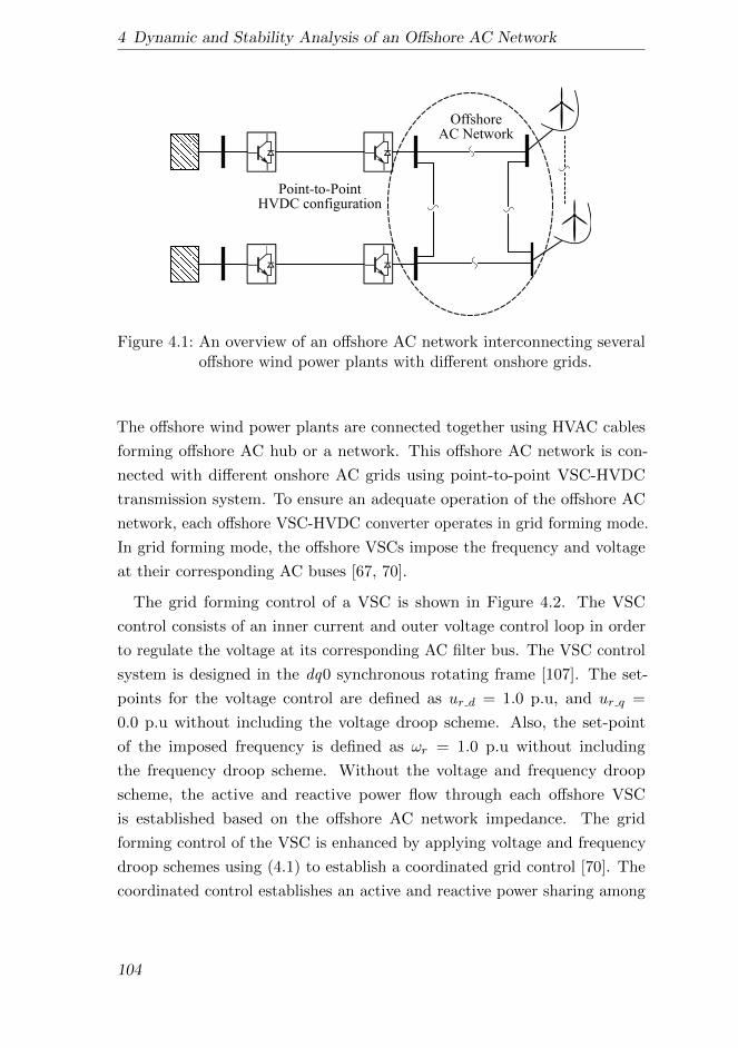
4 Dynamic and Stability Analysis of an Offshore AC Network

OffshoreAC Network

Point-to-PointHVDC configuration

Figure 4.1: An overview of an offshore AC network interconnecting severaloffshore wind power plants with different onshore grids.

The offshore wind power plants are connected together using HVAC cables

forming offshore AC hub or a network. This offshore AC network is con-

nected with different onshore AC grids using point-to-point VSC-HVDC

transmission system. To ensure an adequate operation of the offshore AC

network, each offshore VSC-HVDC converter operates in grid forming mode.

In grid forming mode, the offshore VSCs impose the frequency and voltage

at their corresponding AC buses [67, 70].

The grid forming control of a VSC is shown in Figure 4.2. The VSC

control consists of an inner current and outer voltage control loop in order

to regulate the voltage at its corresponding AC filter bus. The VSC control

system is designed in the dq0 synchronous rotating frame [107]. The set-

points for the voltage control are defined as ur d = 1.0 p.u, and ur q =

0.0 p.u without including the voltage droop scheme. Also, the set-point

of the imposed frequency is defined as ωr = 1.0 p.u without including

the frequency droop scheme. Without the voltage and frequency droop

scheme, the active and reactive power flow through each offshore VSC

is established based on the offshore AC network impedance. The grid

forming control of the VSC is enhanced by applying voltage and frequency

droop schemes using (4.1) to establish a coordinated grid control [70]. The

coordinated control establishes an active and reactive power sharing among

104

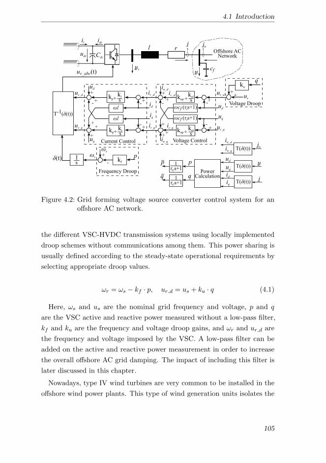
4.1 Introduction

i

udc

l r

cf

Cdc

il idc

kp+ki

s

+

-+

+-

+-

++

+

T-1( (t))

in

id

iq

ud

uq

1s

kf

+

-

s

p

T( (t))

ud

uq

id

iq

q

p

PowerCalculation

uv_abc(t)

l

l

T( (t))

T( (t))

uvu

in

u

i

cs+11

cs+11

kp+ki

s

kop +koi

s

in_d

in_q

ud

uq

ur_d

ur_q

ku

q

kop +koi

s

(t)

cf ( is+1)

+-

-+

+

+

+

++

-

+

cf ( is+1)

ir_d

ir_q

Current Control Voltage Control

uv_d

uv_q

+ us

Voltage Droop

r

Frequency Droop

Offshore ACNetwork

ic_d

ic_q

in_d

in_q

q

p

Figure 4.2: Grid forming voltage source converter control system for anoffshore AC network.

the different VSC-HVDC transmission systems using locally implemented

droop schemes without communications among them. This power sharing is

usually defined according to the steady-state operational requirements by

selecting appropriate droop values.

ωr = ωs − kf · p, ur d = us + ku · q (4.1)

Here, ωs and us are the nominal grid frequency and voltage, p and q

are the VSC active and reactive power measured without a low-pass filter,

kf and ku are the frequency and voltage droop gains, and ωr and ur d are

the frequency and voltage imposed by the VSC. A low-pass filter can be

added on the active and reactive power measurement in order to increase

the overall offshore AC grid damping. The impact of including this filter is

later discussed in this chapter.

Nowadays, type IV wind turbines are very common to be installed in the

offshore wind power plants. This type of wind generation units isolates the

105

4 Dynamic and Stability Analysis of an Offshore AC Network

offshore AC network from the turbine generator inertia. Also the offshore

AC network is isolated from the onshore synchronous generators inertia

due to the VSC-HVDC transmission systems. For such a network, the

grid frequency would be the average of the imposed frequencies by the grid

forming converters [108]. The frequency of the network (ω) can be calculated

using (4.2).

ω =1

z

z∑i=1

ωr i (4.2)

Here, ωr i is the frequency imposed by the ith VSC, and z is the total

number of grid forming VSCs in the network.

In a stable system, all the frequencies of the grid forming converters

converge at the same equilibrium value in steady-state, and the power is

shared according to the droop values. Generally, the droop values are selected

according to the steady-state operational requirements. These droop gains

not only affect the steady-state power sharing but also the offshore AC

network stability. Therefore, the selection of the droop values is crucial to

ensure both the network stability and an adequate dynamic performance

[109]. In Chapter 3, the method of selecting frequency and voltage droop

gains have been presented from the prospective of the steady-state operation.

However, the boundary of these droop gains are required to be determined

in which an offshore AC network remain stable. This can be achieved by

performing a small signal analysis on an offshore AC network.

4.2 Offshore AC Network Small-Signal Modeling

A linearized system model is best suitable to apply the linear control theory

for small-signal analysis. For z grid forming converters in the offshore

AC network, the complete network open loop small-signal model can be

developed according to the block diagram shown in Figure 4.3. The small

signal model of an offshore AC network is split into two sub-models. Firstly,

a VSC model that includes the differential equations of the converter AC

filter busbar voltage and the VSC control equations. Secondly, an offshore

106

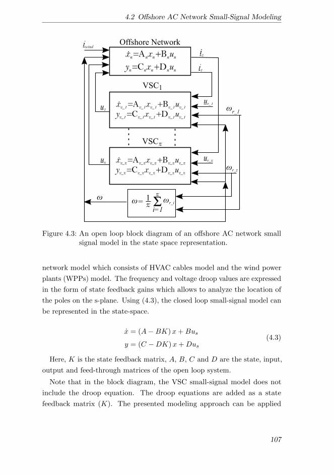
4.2 Offshore AC Network Small-Signal Modeling

Offshore Network

VSC1

VSCz

r_1

xn=Anxn+Bnunyn=Cnxn+Dnun

xv_z=Av_zxv_z+Bv_zuv_zyv_z=Cv_zxv_z+Dv_zuv_z

ur_z

iwind

r_z

xv_1=Av_1xv_1+Bv_1uv_1yv_1=Cv_1xv_1+Dv_1uv_1

uz

u1ur_1

i1

iz

= S1z

i=1z r_i

Figure 4.3: An open loop block diagram of an offshore AC network smallsignal model in the state space representation.

network model which consists of HVAC cables model and the wind power

plants (WPPs) model. The frequency and voltage droop values are expressed

in the form of state feedback gains which allows to analyze the location of

the poles on the s-plane. Using (4.3), the closed loop small-signal model can

be represented in the state-space.

x = (A−BK)x+Bus

y = (C −DK)x+Dus(4.3)

Here, K is the state feedback matrix, A, B, C and D are the state, input,

output and feed-through matrices of the open loop system.

Note that in the block diagram, the VSC small-signal model does not

include the droop equation. The droop equations are added as a state

feedback matrix (K). The presented modeling approach can be applied

107

4 Dynamic and Stability Analysis of an Offshore AC Network

easily on the large network. The model of individual components such as

converter, cable, and wind turbine can be modified and extended without

affecting other component models. Further, the system closed loop poles

trajectory can be analyzed with respect to only droop gains. The complete

model is formulated in the state-space form so that the system stability

can be determined using an eigenvalue analysis of the closed loop matrix

(Acl = A−BK). A system is stable if the real part of all the eigenvalues of

the closed loop state matrix lie on the left half of the s-plane.

4.2.1 VSC Small-Signal Model

The small-signal model of the VSC has been developed based on the control

system shown in Figure 4.2. The analysis is mainly focused on the impact

of frequency and voltage droop on the network stability. Therefore, the

dynamics of the DC side of the HVDC system are not included in the small

signal model. It is considered that the stability of the DC link is ensured

by the DC voltage control of the onshore VSC and the voltages are within

the operational limits. Thus, the small-signal model contains the dynamic

equations of the controlled AC busbar, and the VSC current and voltage

control equations.

Dynamics of VSC Controlled AC Busbar: In grid forming mode, the VSC

controls the voltage at the point of common coupling (PCC) that connects

the VSC substation with rest of the offshore network. The dynamics of

the PCC bus voltage can be derived from the differential equations of the

capacitor connected to it. This capacitor can be defined as an equivalent

offshore network cable capacitance at the controlling busbar or as an added

filter capacitance installed at the offshore substation [31]. The voltage

differential equations of the VSC controlled busbar can be defined as (4.4).

dunddt

=1

cf(ind + inn d − uq0cf (ω0 − ω) + ω0cfu

nq )

dunqdt

=1

cf(inq + inn q + ud0cf (ω0 − ω)− ω0cfu

nd )

(4.4)

108

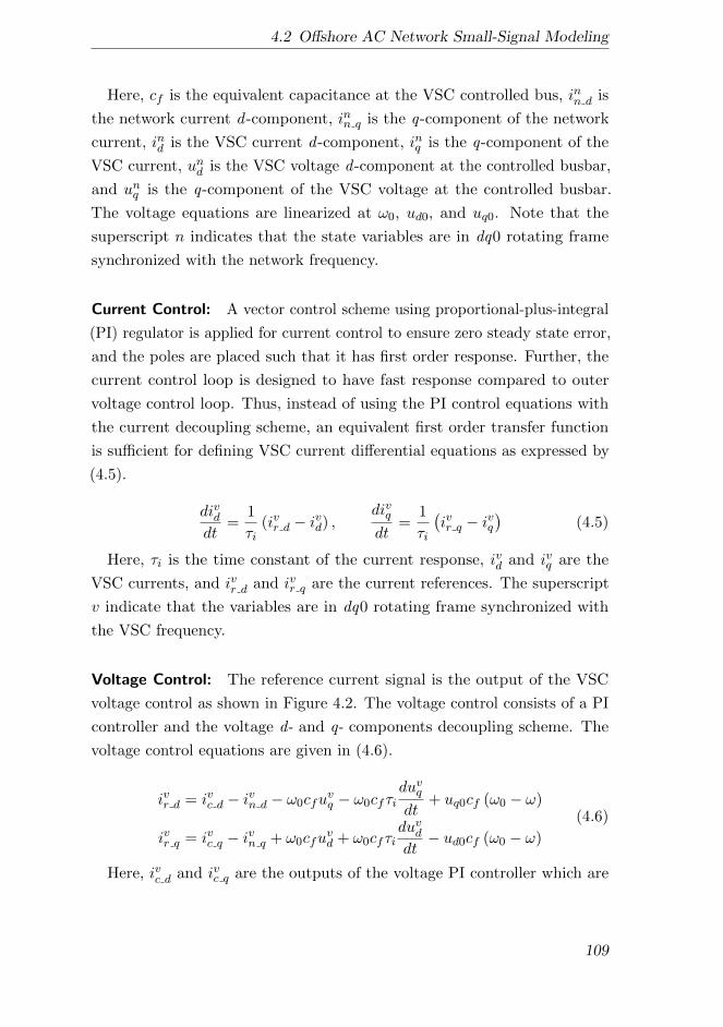
4.2 Offshore AC Network Small-Signal Modeling

Here, cf is the equivalent capacitance at the VSC controlled bus, inn d is

the network current d -component, inn q is the q-component of the network

current, ind is the VSC current d -component, inq is the q-component of the

VSC current, und is the VSC voltage d -component at the controlled busbar,

and unq is the q-component of the VSC voltage at the controlled busbar.

The voltage equations are linearized at ω0, ud0, and uq0. Note that the

superscript n indicates that the state variables are in dq0 rotating frame

synchronized with the network frequency.

Current Control: A vector control scheme using proportional-plus-integral

(PI) regulator is applied for current control to ensure zero steady state error,

and the poles are placed such that it has first order response. Further, the

current control loop is designed to have fast response compared to outer

voltage control loop. Thus, instead of using the PI control equations with

the current decoupling scheme, an equivalent first order transfer function

is sufficient for defining VSC current differential equations as expressed by

(4.5).

divddt

=1

τi(ivr d − ivd) ,

divqdt

=1

τi

(ivr q − ivq

)(4.5)

Here, τi is the time constant of the current response, ivd and ivq are the

VSC currents, and ivr d and ivr q are the current references. The superscript

v indicate that the variables are in dq0 rotating frame synchronized with

the VSC frequency.

Voltage Control: The reference current signal is the output of the VSC

voltage control as shown in Figure 4.2. The voltage control consists of a PI

controller and the voltage d- and q- components decoupling scheme. The

voltage control equations are given in (4.6).

ivr d = ivc d − ivn d − ω0cfuvq − ω0cfτi

duvqdt

+ uq0cf (ω0 − ω)

ivr q = ivc q − ivn q + ω0cfuvd + ω0cfτi

duvddt− ud0cf (ω0 − ω)

(4.6)

Here, ivc d and ivc q are the outputs of the voltage PI controller which are

109

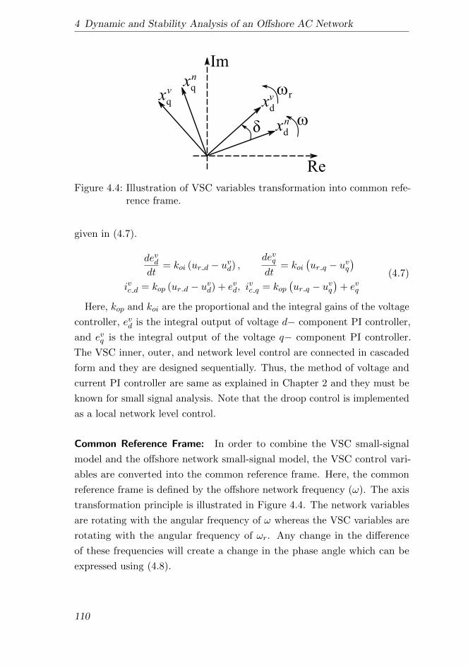
4 Dynamic and Stability Analysis of an Offshore AC Network

xdv

xqn

xdn

xqv r

Re

Im

Figure 4.4: Illustration of VSC variables transformation into common refe-rence frame.

given in (4.7).

devddt

= koi (ur d − uvd) ,devqdt

= koi(ur q − uvq

)ivc d = kop (ur d − uvd) + evd, i

vc q = kop

(ur q − uvq

)+ evq

(4.7)

Here, kop and koi are the proportional and the integral gains of the voltage

controller, evd is the integral output of voltage d− component PI controller,

and evq is the integral output of the voltage q− component PI controller.

The VSC inner, outer, and network level control are connected in cascaded

form and they are designed sequentially. Thus, the method of voltage and

current PI controller are same as explained in Chapter 2 and they must be

known for small signal analysis. Note that the droop control is implemented

as a local network level control.

Common Reference Frame: In order to combine the VSC small-signal

model and the offshore network small-signal model, the VSC control vari-

ables are converted into the common reference frame. Here, the common

reference frame is defined by the offshore network frequency (ω). The axis

transformation principle is illustrated in Figure 4.4. The network variables

are rotating with the angular frequency of ω whereas the VSC variables are

rotating with the angular frequency of ωr. Any change in the difference

of these frequencies will create a change in the phase angle which can be

expressed using (4.8).

110

4.2 Offshore AC Network Small-Signal Modeling

dδ

dt= ωr − ω (4.8)

The transformation between these two frames can be done using (4.9).

The rotation matrix (R (δ)) is orthogonal. It is derived from Euler formula

and posses the property of R (δ) ·R−1 (δ) = I.

xv = R (δ)xn[xvdxvq

]=

[cos(δ) sin(δ)

− sin(δ) cos(δ)

][xndxnq

](4.9)

Here, xnd and xnq are variables rotating with the network frequency, xvd and

xvq are variables rotating with the VSC imposed frequency, and δ is the phase

angle between these two references. To be used in a linear small-signal model,

the above transformation equation can be linearized at the equilibrium point

of δ0, xd0, and xq0. It is considered that both frames are initially aligned,

thus the linearized VSCs variables in the common frame can be defined

using (4.10).

xvd = xnd + xq0δ ∵ δ0 = 0

xvq = xnq − xd0δ(4.10)

The voltage state variables in the VSC voltage control equation can

be transformed into the common frame using above equation as (4.11).

Here, the voltage equilibrium points are set as xd0 = ud0 = 1.0 p.u, and

xq0 = uq0 = 0.0 p.u by considering a flat-start of the network.

uvd = und

uvq = unq − ud0δ(4.11)

Similarly, assuming that there is no current flowing at the equilibrium

point (flat-start) i.e xd0 = id0 = 0.0 p.u, and xq0 = iq0 = 0.0 p.u. Then, the

current state variables in the VSC current and voltage control equation can

be transformed in the common frame using (4.12).

111

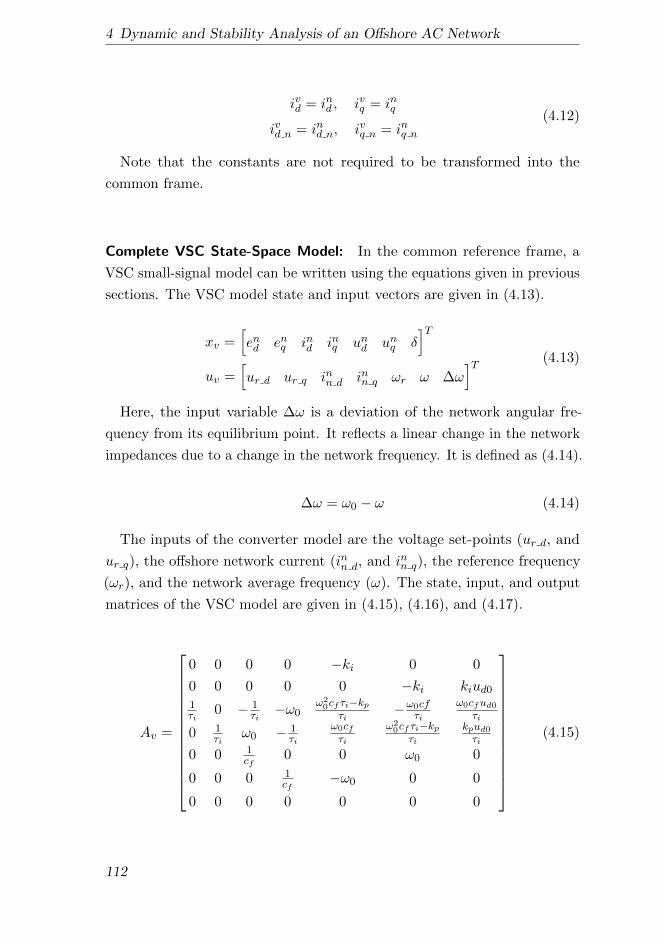
4 Dynamic and Stability Analysis of an Offshore AC Network

ivd = ind , ivq = inq

ivd n = ind n, ivq n = inq n(4.12)

Note that the constants are not required to be transformed into the

common frame.

Complete VSC State-Space Model: In the common reference frame, a

VSC small-signal model can be written using the equations given in previous

sections. The VSC model state and input vectors are given in (4.13).

xv =[end enq ind inq und unq δ

]Tuv =

[ur d ur q inn d inn q ωr ω ∆ω

]T (4.13)

Here, the input variable ∆ω is a deviation of the network angular fre-

quency from its equilibrium point. It reflects a linear change in the network

impedances due to a change in the network frequency. It is defined as (4.14).

∆ω = ω0 − ω (4.14)

The inputs of the converter model are the voltage set-points (ur d, and

ur q), the offshore network current (inn d, and inn q), the reference frequency

(ωr), and the network average frequency (ω). The state, input, and output

matrices of the VSC model are given in (4.15), (4.16), and (4.17).

Av =

0 0 0 0 −ki 0 0

0 0 0 0 0 −ki kiud0

1τi

0 − 1τi−ω0

ω20cf τi−kp

τi−ω0cf

τi

ω0cfud0τi

0 1τi

ω0 − 1τi

ω0cfτi

ω20cf τi−kp

τi

kpud0τi

0 0 1cf

0 0 ω0 0

0 0 0 1cf

−ω0 0 0

0 0 0 0 0 0 0

(4.15)

112

4.2 Offshore AC Network Small-Signal Modeling

Bv =

ki 0 0 0 0 0 0

0 ki 0 0 0 0 0kpτi

0 − 1τi−ω0 cfud0ω0 −cfud0ω0

−τicfud0ω0+cfuq0τi

0kpτi

ω0 − 1τi

0 0−τicfuq0ω0−cfud0

τi

0 0 1cf

0 0 0 −uq00 0 0 1

cf0 0 ud0

0 0 0 0 1 −1 0

(4.16)

Cv = I(7x7), Dv = 0 (4.17)

4.2.2 Offshore Network Small-Signal Model

A small-signal model of the offshore AC network can be constructed by

combining the branches current and voltage differential equations using

(4.18) and (4.19).

[ind kinq k

]=

[− rl ω0

−ω0 − rl

][ind kinq k

]+

[1l 0 −iq00 1

l id0

]∆und k∆unq k∆ω

(4.18)

Here, ind k and inq k are the currents of the branch in the common reference

frame. The voltages across the branch element are defined as ∆und k =

und m+1 − und m and ∆unq k = unq m+1 − unq m. Also, ∆ω is the frequency

deviation from its equilibrium point and it can be calculated using (4.14).

[und munq m

]=

[0 ω0

−ω0 0

][und munq m

]+

[1c 0 −uq00 1

c ud0

]∆ind m∆inq m∆ω

(4.19)

Here, und m and unq m are the voltages of the branch in the common reference

frame. The currents injected into the busbar are defined as ∆ind m = ind k+1 +

ind k + ind wind, and ∆inq m = inq k+1 + inq k + inq wind.

It is assumed that type IV wind turbines are installed at the offshore

wind power plants which can control the active and the reactive power

independently. Since the focus of the study is on the droop effects and not

113

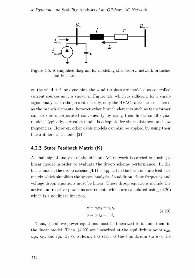
4 Dynamic and Stability Analysis of an Offshore AC Network

um+1

um

r

ik+1

iwind c

l

ik

Figure 4.5: A simplified diagram for modeling offshore AC network branchesand busbars.

on the wind turbine dynamics, the wind turbines are modeled as controlled

current sources as it is shown in Figure 4.5, which is sufficient for a small-

signal analysis. In the presented study, only the HVAC cables are considered

as the branch elements, however other branch elements such as transformer

can also be incorporated conveniently by using their linear small-signal

model. Typically, a π-cable model is adequate for short distances and low

frequencies. However, other cable models can also be applied by using their

linear differential model [24].

4.2.3 State Feedback Matrix (K)

A small-signal analysis of the offshore AC network is carried out using a

linear model in order to evaluate the droop scheme performance. In the

linear model, the droop scheme (4.1) is applied in the form of state feedback

matrix which simplifies the system analysis. In addition, these frequency and

voltage droop equations must be linear. These droop equations include the

active and reactive power measurements which are calculated using (4.20)

which is a nonlinear function.

p = udid + uqiq

q = uqid − udiq(4.20)

Thus, the above power equations must be linearized to include them in

the linear model. Then, (4.20) are linearized at the equilibrium point ud0,

uq0, id0, and iq0. By considering flat start as the equilibrium state of the

114

4.2 Offshore AC Network Small-Signal Modeling

offshore AC network, the linear droop equations for the small-signal model

can be written as (4.21).

ωr = ωs − kf ind , ∵ p = id

ur d = us − kuinq , ∵ q = −iq(4.21)

Here, ind , and inq are the VSC current dq- components in common reference

frame. The state feedback matrix can be defined using (4.22) for z grid

forming VSCs. The closed loop system is a multi-input multi-output (MIMO)

system and K is not a full state feedback matrix.

Kx =

kf 1 0 · · · 0

0 ku 1

.... . .

...

kf z 0

0 · · · 0 ku z

ind 1

inq 1...

ind zinq z

(4.22)

Here, x is the state vector and K is the state feedback matrix. Note that

the matrix K is defined without including a low-pass filter at the active and

reactive power measurements. Without including the low-pass filter, the

network voltage and frequency may have an oscillatory behavior due to the

droop schemes. In order to increase damping in the system, a low-pass filter

is included on the power measurements. The droop equations including the

low-pass filter can be defined as:

ωr = ωs − kf p, ∵ p =ωc

s+ ωcp

ur d = us + kuq, ∵ q =ωc

s+ ωcq

(4.23)

Here, ωc = 1/τc is the cutoff frequency of the low pass filters, and p, q

are the filtered active and reactive power outputs. Note that p = ind , and

q = −inq for the linearized small-signal model.

115

4 Dynamic and Stability Analysis of an Offshore AC Network

u3 u

1 VSC-1

VSC-2u2

l13

l23

i2

r13

r23

i1i

13

i23

iwind

r

r

l

l

VSC System 1

VSC System 2

Cable 1

Cable 2

c3* c3*

c3* c3*

cf*

cf*

Figure 4.6: Offshore AC network having two frequency controlled voltagesource converter.

4.3 Case Study

In this section, a small-signal analysis of the network shown in Figure 4.6 is

performed using the proposed method. The offshore AC network has two

VSCs and an equivalent wind power plant. In the presented case study, each

VSC system is connected with the AC hub bus (u3) using HVAC cables.

The length of the cables are 10 km each [11]. The network and control

parameters are given in Table 4.1. The cable parameters are taken from the

manufacturer data sheet listed in [102, 110]. Note that the filter capacitance

value in the VSC small-signal model is cf = c∗f + c∗3, and the equivalent

capacitance at the AC hub bus is c = c∗3 + c∗3. Where, c∗3 is the half of the

total cable capacitance, r13, r23 are the total cable resistances, and l13, l23

are the total cable inductances.

At first, a complete closed loop system small-signal model is obtained using

the proposed method. The closed loop system is defined in a state-space

form as given in (4.3). The eigenvalue analysis can then be performed using

the state matrix. The small-signal analysis determines the frequency and

voltage droop values at which the system becomes unstable. Finally, the

dynamic performance of the system and the stability conditions are validated

by performing a nonlinear simulation in Simulink SimPowerSystems.

116

4.3 Case Study

Table 4.1: Offshore AC network and control parameters for stability analysis

Variables Value Unit

Rated voltage 220 kV

Rated apparent power 500 MVA

Nominal angular frequency (ω) 314.16 rad/s

Cable resistance 0.032 Ω/km

Cable inductance 0.4 mH/km

Cable capacitance 0.17 µF/km

Length of cables 1, and 2 10 km

Filter capacitance(c∗f)

3.29 µF

VSC reactor resistance 0.5 mΩ

VSC reactor inductance 55.0 mH

VSC voltage control gain 0.3 + 0.15s

p.u

VSC current time constant (τi) 0.002 s

Cutoff frequency of low-pass filter (ωc) 25 rad/s

4.3.1 Formation of Complete System Model

The analytic procedure of connecting offshore network and VSCs model

is explained here to form the complete system model in the state-space

representation. The complete model can also be formed by using computati-

onal tools such as a MATLAB function ‘linmod’. The function obtains a

linear model of the system expressed as Figure 4.3 described in the Simulink

model. The input and output of the complete system must be assigned using

Simulink input and output port blocks.

In order to formulate the system complete model analytically, the resultant

state vector of the network can be written as (4.24). Note that the frame

superscript label is removed since both VSCs and offshore network model

are in common reference frame.

x =[x1 x2 x3

]x1 =

[ed 1 eq 1 id 1 iq 1 ud 1 uq 1 δ1

]Tx2 =

[ed 2 eq 2 id 2 iq 2 ud 2 uq 2 δ2

]Tx3 =

[id 13 iq 13 ud 3 uq 3 id 23 iq 23

]T(4.24)

117

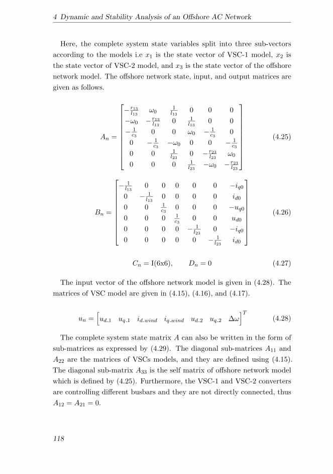
4 Dynamic and Stability Analysis of an Offshore AC Network

Here, the complete system state variables split into three sub-vectors

according to the models i.e x1 is the state vector of VSC-1 model, x2 is

the state vector of VSC-2 model, and x3 is the state vector of the offshore

network model. The offshore network state, input, and output matrices are

given as follows.

An =

− r13l13

ω01l13

0 0 0

−ω0 − r13l13

0 1l13

0 0

− 1c3

0 0 ω0 − 1c3

0

0 − 1c3−ω0 0 0 − 1

c3

0 0 1l23

0 − r23l23

ω0

0 0 0 1l23

−ω0 − r23l23

(4.25)

Bn =

− 1l13

0 0 0 0 0 −iq00 − 1

l130 0 0 0 id0

0 0 1c3

0 0 0 −uq00 0 0 1

c30 0 ud0

0 0 0 0 − 1l23

0 −iq00 0 0 0 0 − 1

l23id0

(4.26)

Cn = I(6x6), Dn = 0 (4.27)

The input vector of the offshore network model is given in (4.28). The

matrices of VSC model are given in (4.15), (4.16), and (4.17).

un =[ud 1 uq 1 id wind iq wind ud 2 uq 2 ∆ω

]T(4.28)

The complete system state matrix A can also be written in the form of

sub-matrices as expressed by (4.29). The diagonal sub-matrices A11 and

A22 are the matrices of VSCs models, and they are defined using (4.15).

The diagonal sub-matrix A33 is the self matrix of offshore network model

which is defined by (4.25). Furthermore, the VSC-1 and VSC-2 converters

are controlling different busbars and they are not directly connected, thus

A12 = A21 = 0.

118

4.3 Case Study

A =

A11 (7x7) A12 (7x7) A13 (7x6)

A21 (7x7) A22 (7x7) A23 (7x6)

A31 (6x7) A32 (6x7) A33 (6x6)

(4.29)

The matrix A13 connects the output of the network current with the input

of VSC-1. The network currents id 13 and iq 13 are the inputs to VSC-1

model. In order to link the offshore network model output with the VSC-1

model inputs, the corresponding columns of matrix Cn given in (4.27) are

multiplied with the corresponding columns of matrix Bv given in (4.16) as:

A13 =[Bv 1(7x2)× Cn 1(2x2) 0(7x4)

]Bv 1 =

[C3 C4

], Cn 1 =

[1 0

0 1

](4.30)

The network current id 23 and iq 23 are the inputs of VSC-2 model. The

matrix A23 can be found in a similar manner as given by (4.31). The

corresponding columns of matrix Bv for matrix Bv 2 are the same as of Bv 1.

The matrix Cn 2 is also an identity matrix.

A23 =[0(7x4) Bv 2(7x2)× Cn 2(2x2)

](4.31)

The matrix A31 connects the output voltage of the VSC-1 model with

the input of the offshore network model, and it can be defined as (4.32).

The state variables ud 1 and uq 1 of the VSC-1 model are the input of

network model, thus the column 1 and 2 of matrix Bn are multiplied by the

corresponding matrix of Cv.

A31 =[0(6x4) Bn 1(6x2)× Cv 1(2x3)

]Bn 1 =

[C1 C2

], Cv 1 =

[1 0 0

0 1 0

](4.32)

Similarly, the matrix A32 links the output voltage of the VSC-2 with the

network model, and its value is calculated using (4.33).

A32 =[0(6x4) Bn 2(6x2)× Cv 2(2x3)

](4.33)

119

4 Dynamic and Stability Analysis of an Offshore AC Network

Here, the matrix column of Cv for Cv 2 are same as of Cv 1 and they are

applied using VSC-2 parameters. The corresponding column indexes of Bn

for VSC-2 are 5 and 6.

The input vector u for the whole system can be defined in a similar manner.

The input vector can be split into two sub-vectors as (4.34).

u =[uvi(6x1) uω(3x1)

]Tuvi =

[ur d1 ur q1 ur d2 ur q2 id wind iq wind

]uω =

[ωr1 ωr2 ω0

] (4.34)

Here, uvi is the input vector containing the voltage set-points of VSCs and

the wind power plant current infeed. uω is the vector of input frequencies.

Thus, the B matrix can be written in the form of sub-matrices as (4.35).

B =

B11(7x2) 0 0 B14(7x3)

0 B22(7x2) 0 B24(7x3)

0 0 B33(6x2) B34(6x3)

(4.35)

The set-points of the VSC-1 and VSC-2 voltage controller are defined

by the matrices B11 and B22 respectively, and their respective columns 1

and 2 are extracted from (4.16). The matrix B33 corresponds to the input

of offshore network model and its respective column indexes are 3 and 4

extracted from (4.26).

The matrix B14 is an input matrix of frequencies for VSC-1 i.e ωr1, ω,

and ∆ω. In order to link the VSC-1 frequency with the network frequency

and VSC-2 frequency, input matrix can be rewritten by applying (4.2) and

(4.14). The input frequencies transformation matrix for VSC-1 is given in

(4.36). ωr1ω∆ω

=

1 0 0

0.5 0.5 0

−0.5 −0.5 1

ωr1ωr2

ω0

(4.36)

Thus, the B14 can be defined by extracting the corresponding columns

from (4.16) and multiplying with the transformation matrix given in (4.36)

120

4.3 Case Study

as

B14 =[C5 C6 C7

] 1 0 0

0.5 0.5 0

−0.5 −0.5 1

(4.37)

The matrix B24 is defined in a similar manner. However, the input

transformation matrix is modified according to VSC-2 input as (4.38).

B24 =[C5 C6 C7

] 0 1 0

0.5 0.5 0

−0.5 −0.5 1

(4.38)

The influence of the change in network frequency on the network elements

in term of frequencies set-points can be defined by multiplying the correspon-

ding column from (4.26) with the input frequency transformation matrix.

Thus, the matrix B34 is calculated using (4.39).

B34 =[C7

] [−0.5 −0.5 1

](4.39)

The vector of output variables define in (4.40) contains state and input

variables.

y =[id 1 iq 1 ud 1 uq 1 id 2 iq 2 ud 2 uq 2 ud 3 uq 3

ω ω1 ω2

]T (4.40)

The state output matrix C is a diagonal matrix whose values are calculated

using (4.17) and (4.27).

121

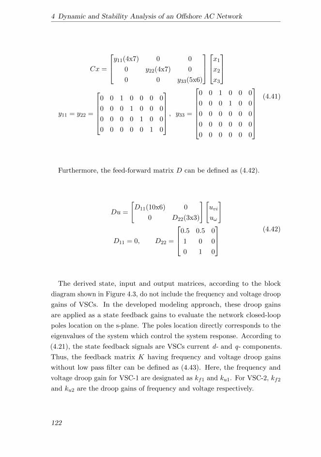
4 Dynamic and Stability Analysis of an Offshore AC Network

Cx =

y11(4x7) 0 0

0 y22(4x7) 0

0 0 y33(5x6)

x1

x2

x3

y11 = y22 =

0 0 1 0 0 0 0

0 0 0 1 0 0 0

0 0 0 0 1 0 0

0 0 0 0 0 1 0

, y33 =

0 0 1 0 0 0

0 0 0 1 0 0

0 0 0 0 0 0

0 0 0 0 0 0

0 0 0 0 0 0

(4.41)

Furthermore, the feed-forward matrix D can be defined as (4.42).

Du =

[D11(10x6) 0

0 D22(3x3)

][uvi

uω

]

D11 = 0, D22 =

0.5 0.5 0

1 0 0

0 1 0

(4.42)

The derived state, input and output matrices, according to the block

diagram shown in Figure 4.3, do not include the frequency and voltage droop

gains of VSCs. In the developed modeling approach, these droop gains

are applied as a state feedback gains to evaluate the network closed-loop

poles location on the s-plane. The poles location directly corresponds to the

eigenvalues of the system which control the system response. According to

(4.21), the state feedback signals are VSCs current d- and q- components.

Thus, the feedback matrix K having frequency and voltage droop gains

without low pass filter can be defined as (4.43). Here, the frequency and

voltage droop gain for VSC-1 are designated as kf1 and ku1. For VSC-2, kf2

and ku2 are the droop gains of frequency and voltage respectively.

122

4.3 Case Study

K =

0 0 0 ku1 0 0 0 0 0 0 0

0 0 0 0 0 0 0 0 0 0 0

0 0 kf1 0 0 0 0 0 0 0 0

0 0 0 0 0 0 0 0 0 0 ku2

0 0 0 0 0 0 0 0 0 0 0

0 0 0 0 0 0 0 0 0 kf2 0

0 0 0 0 0 0 0 0 0 0 0

0 0 0 0 0 0 0 0 0 0 0

0 0 0 0 0 0 0 0 0 0 0

0(9x9)

(4.43)

The closed loop state matrix given in (4.3) can now be computed to

analyze the system dynamics and its stability.

4.3.2 Eigenvalue Analysis

Using an eigenvalue (λ) analysis, the closed loop system poles and zeros

can be plotted on the s-plane as shown in Figure 4.7. In Figure 4.7, the

poles and zeroes of the system are plotted using the following droop values:

kf1 = 0.00165 p.u (VSC-1 frequency droop), ku1 = 0.0020 p.u (VSC-1 voltage

droop), kf2 = 0.00231 p.u (VSC-2 frequency droop), and ku2 = −0.0020 p.u

(VSC-2 voltage droop). As observed from the plot, the system is stable since

the real parts of all eigenvalues are negative.

There are two sets of poles that are influenced by the droop gains. One set

is mainly affected by the frequency droop gain and the other is influenced

by the voltage droop gain. To observe the influence of the frequency droop

gain on the system poles, the trajectories of the poles map are shown in

Figure 4.8a. These trajectories are generated by varying only the VSC-

1 frequency droop gain as 0.0 ≤ kf1 ≤ 0.01 p.u while keeping the other

parameters constant. In the plot, the poles move along the gradient from

blue (kf1 = 0.0 p.u) to red (kf1 = 0.01 p.u). It can be observed that the

poles located close to −0.5 and −50 of the real axis scale are dominant and

lead the system into instability for kf1 ≥ 0.003 p.u. The poles located close

to −200 of the real axis scale are not importantly affected by the frequency

123

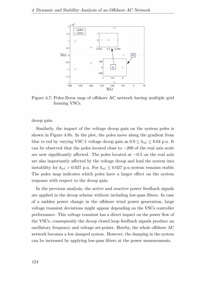
4 Dynamic and Stability Analysis of an Offshore AC Network

300 250 200 150 100 50 0 502

1.5

1

0.5

0

0.5

1

1.5

2x 10

4

1 0.5 0

200

0

200

0.502 0.5 0.4981

0

1

poleszeros

Figure 4.7: Poles-Zeros map of offshore AC network having multiple gridforming VSCs.

droop gain.

Similarly, the impact of the voltage droop gain on the system poles is

shown in Figure 4.8b. In the plot, the poles move along the gradient from

blue to red by varying VSC-1 voltage droop gain as 0.0 ≤ ku1 ≤ 0.04 p.u. It

can be observed that the poles located close to −200 of the real axis scale

are now significantly affected. The poles located at −0.5 on the real axis

are also importantly affected by the voltage droop and lead the system into

instability for ku1 > 0.027 p.u. For ku1 ≤ 0.027 p.u system remains stable.

The poles map indicates which poles have a larger effect on the system

response with respect to the droop gain.

In the previous analysis, the active and reactive power feedback signals

are applied in the droop scheme without including low-pass filters. In case

of a sudden power change in the offshore wind power generation, large

voltage transient deviations might appear depending on the VSCs controller

performance. This voltage transient has a direct impact on the power flow of

the VSCs, consequently the droop closed loop feedback signals produce an

oscillatory frequency and voltage set-points. Hereby, the whole offshore AC

network becomes a low damped system. However, the damping in the system

can be increased by applying low-pass filters at the power measurements.

124

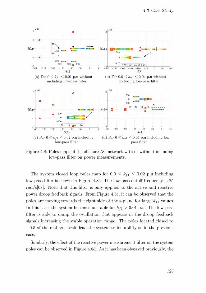
4.3 Case Study

300 250 200 150 100 50 0 502

1

0

1

2x 10

4

( )

( )

202 200 198

5000

0

5000

(a) For 0 ≤ kf1 ≤ 0.01 p.u withoutincluding low-pass filter

300 250 200 150 100 50 0 50 1002

1

0

1

2x 10

5

0.505 0.5 0.495 0.490.02

0

0.02( )

( )

(b) For 0.0 ≤ ku1 ≤ 0.04 p.u withoutincluding low-pass filter

300 250 200 150 100 50 0 502

1

0

1

2x 10

4

20 10 0 10

200

0

200

( )

(c) For 0 ≤ kf1 ≤ 0.02 p.u includinglow-pass filter

300 250 200 150 100 50 0 502

1

0

1

2x 10

5

60 40 20 0

200

0

200

( )

( )

(d) For 0 ≤ ku1 ≤ 0.04 p.u including lowpass filter

Figure 4.8: Poles maps of the offshore AC network with or without includinglow-pass filter on power measurements.

The system closed loop poles map for 0.0 ≤ kf1 ≤ 0.02 p.u including

low-pass filter is shown in Figure 4.8c. The low-pass cutoff frequency is 25

rad/s[68]. Note that this filter is only applied to the active and reactive

power droop feedback signals. From Figure 4.8c, it can be observed that the

poles are moving towards the right side of the s-plane for large kf1 values.

In this case, the system becomes unstable for kf1 > 0.01 p.u. The low-pass

filter is able to damp the oscillation that appears in the droop feedback

signals increasing the stable operation range. The poles located closed to

−0.5 of the real axis scale lead the system to instability as in the previous

case.

Similarly, the effect of the reactive power measurement filter on the system

poles can be observed in Figure 4.8d. As it has been observed previously, the

125

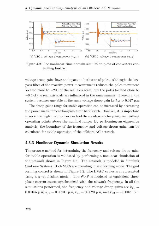
4 Dynamic and Stability Analysis of an Offshore AC Network

5.9 6.0 6.1 6.2 6.3 6.4 6.50.997

0.998

0.999

1.000

1.001

1.002

Time (sec)

Volt

age

(p.u

)

Without Low Pass Filter

With Low Pass Filter

(a) VSC-1 voltage d-component (ud 1)

5.9 6.0 6.1 6.2 6.3 6.4 6.50.997

0.998

0.999

1.000

1.001

1.002

Time (sec)

Volt

age

(p.u

)

Without Low Pass Filter

With Low Pass Filter

(b) VSC-2 voltage d-component (ud 2)

Figure 4.9: The nonlinear time domain simulation plots of converters con-trolling busbar.

voltage droop gains have an impact on both sets of poles. Although, the low-

pass filter of the reactive power measurement reduces the poles movement

located close to −200 of the real axis scale, but the poles located close to

−0.5 of the real axis scale are influenced in the same manner. Therefore, the

system becomes unstable at the same voltage droop gain i.e ku1 > 0.027 p.u.

The droop gains range for stable operation can be increased by decreasing

the power measurement low-pass filter bandwidth. However, it is important

to note that high droop values can lead the steady-state frequency and voltage

operating points above the nominal range. By performing an eigenvalue

analysis, the boundary of the frequency and voltage droop gains can be

calculated for stable operation of the offshore AC network.

4.3.3 Nonlinear Dynamic Simulation Results

The propose method for determining the frequency and voltage droop gains

for stable operation is validated by performing a nonlinear simulation of

the network shown in Figure 4.6. The network is modeled in Simulink

SimPowerSystems. Both VSCs are operating in grid forming mode. The grid

forming control is shown in Figure 4.2. The HVAC cables are represented

using a π−equivalent model. The WPP is modeled as equivalent three-

phase current source synchronized with the network frequency. In all the

simulations performed, the frequency and voltage droop gains are kf1 =

0.00165 p.u, kf2 = 0.00231 p.u, ku1 = 0.0020 p.u, and ku2 = −0.0020 p.u,

126

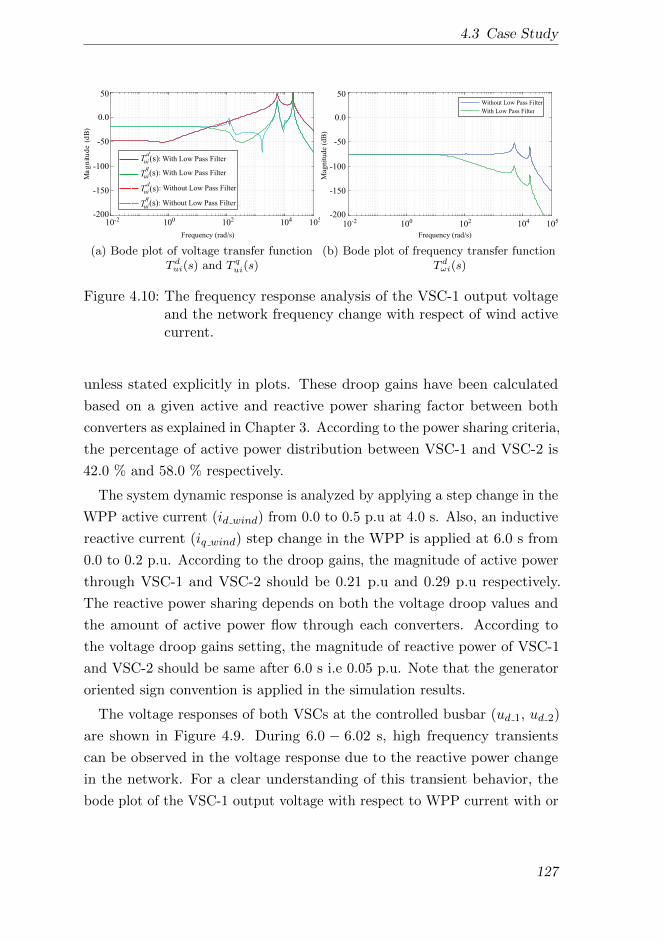
4.3 Case Study

Ma

gn

itu

de

(d

B)

Frequency (rad/s)

: With Low Pass FilterTuid(s)

: With Low Pass FilterqTui(s)

: Without Low Pass FilterTuid(s)

: Without Low Pass FilterqTui(s)

50

0.0

-50

-150

-200

-100

10-2 100 102 104 105

(a) Bode plot of voltage transfer functionT dui(s) and T q

ui(s)

Mag

nit

ud

e (d

B)

Frequency (rad/s)

10-2 100 102 104 105

50

0.0

-50

-150

-200

-100

Without Low Pass Filter

With Low Pass Filter

(b) Bode plot of frequency transfer functionT dωi(s)

Figure 4.10: The frequency response analysis of the VSC-1 output voltageand the network frequency change with respect of wind activecurrent.

unless stated explicitly in plots. These droop gains have been calculated

based on a given active and reactive power sharing factor between both

converters as explained in Chapter 3. According to the power sharing criteria,

the percentage of active power distribution between VSC-1 and VSC-2 is

42.0 % and 58.0 % respectively.

The system dynamic response is analyzed by applying a step change in the

WPP active current (id wind) from 0.0 to 0.5 p.u at 4.0 s. Also, an inductive

reactive current (iq wind) step change in the WPP is applied at 6.0 s from

0.0 to 0.2 p.u. According to the droop gains, the magnitude of active power

through VSC-1 and VSC-2 should be 0.21 p.u and 0.29 p.u respectively.

The reactive power sharing depends on both the voltage droop values and

the amount of active power flow through each converters. According to

the voltage droop gains setting, the magnitude of reactive power of VSC-1

and VSC-2 should be same after 6.0 s i.e 0.05 p.u. Note that the generator

oriented sign convention is applied in the simulation results.

The voltage responses of both VSCs at the controlled busbar (ud 1, ud 2)

are shown in Figure 4.9. During 6.0 − 6.02 s, high frequency transients

can be observed in the voltage response due to the reactive power change

in the network. For a clear understanding of this transient behavior, the

bode plot of the VSC-1 output voltage with respect to WPP current with or

127

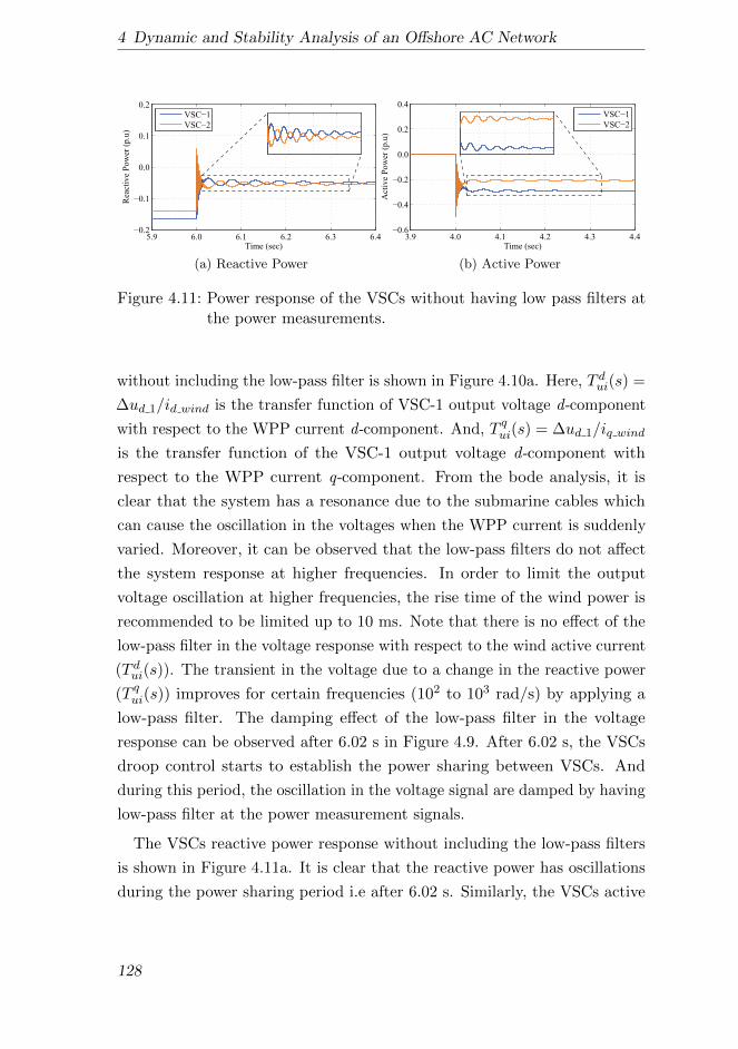
4 Dynamic and Stability Analysis of an Offshore AC Network

5.9 6.0 6.1 6.2 6.3 6.40.2

0.1

0.0

0.1

0.2

Time (sec)

Rea

ctiv

e P

ow

er (

p.u

)VSC 1

VSC 2

(a) Reactive Power

3.9 4.0 4.1 4.2 4.3 4.40.6

0.4

0.2

0.0

0.2

0.4

Time (sec)

Act

ive

Pow

er (

p.u

)

VSC 1

VSC 2

(b) Active Power

Figure 4.11: Power response of the VSCs without having low pass filters atthe power measurements.

without including the low-pass filter is shown in Figure 4.10a. Here, T dui(s) =

∆ud 1/id wind is the transfer function of VSC-1 output voltage d-component

with respect to the WPP current d-component. And, T qui(s) = ∆ud 1/iq wind

is the transfer function of the VSC-1 output voltage d-component with

respect to the WPP current q-component. From the bode analysis, it is

clear that the system has a resonance due to the submarine cables which

can cause the oscillation in the voltages when the WPP current is suddenly

varied. Moreover, it can be observed that the low-pass filters do not affect

the system response at higher frequencies. In order to limit the output

voltage oscillation at higher frequencies, the rise time of the wind power is

recommended to be limited up to 10 ms. Note that there is no effect of the

low-pass filter in the voltage response with respect to the wind active current

(T dui(s)). The transient in the voltage due to a change in the reactive power

(T qui(s)) improves for certain frequencies (102 to 103 rad/s) by applying a

low-pass filter. The damping effect of the low-pass filter in the voltage

response can be observed after 6.02 s in Figure 4.9. After 6.02 s, the VSCs

droop control starts to establish the power sharing between VSCs. And

during this period, the oscillation in the voltage signal are damped by having

low-pass filter at the power measurement signals.

The VSCs reactive power response without including the low-pass filters

is shown in Figure 4.11a. It is clear that the reactive power has oscillations

during the power sharing period i.e after 6.02 s. Similarly, the VSCs active

128

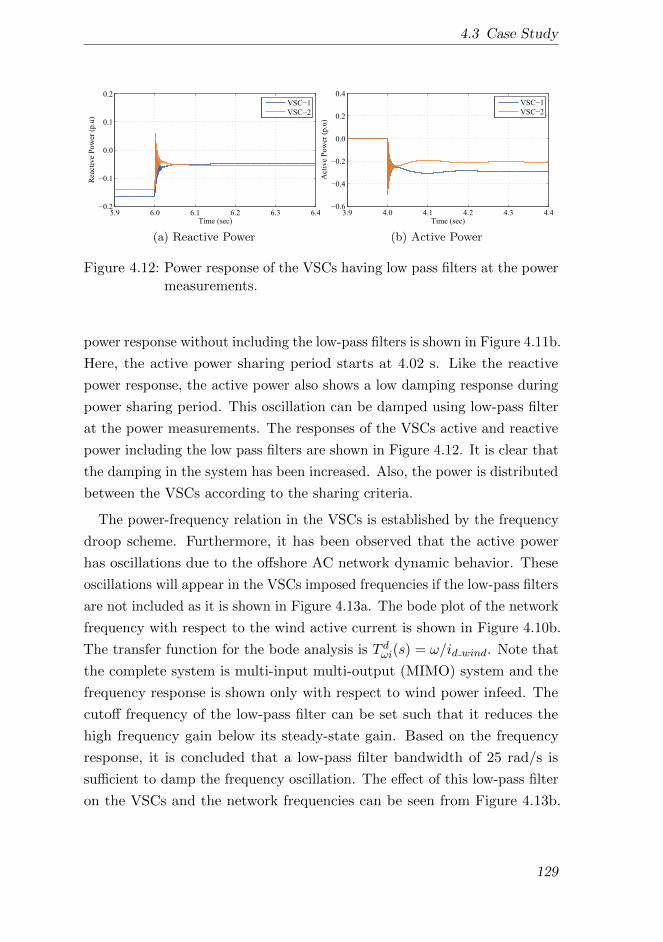
4.3 Case Study

5.9 6.0 6.1 6.2 6.3 6.40.2

0.1

0.0

0.1

0.2

Time (sec)

Rea

ctiv

e P

ow

er (

p.u

)

VSC 1

VSC 2

(a) Reactive Power

3.9 4.0 4.1 4.2 4.3 4.40.6

0.4

0.2

0.0

0.2

0.4

Time (sec)

Act

ive

Pow

er (

p.u

)

VSC 1

VSC 2

(b) Active Power

Figure 4.12: Power response of the VSCs having low pass filters at the powermeasurements.

power response without including the low-pass filters is shown in Figure 4.11b.

Here, the active power sharing period starts at 4.02 s. Like the reactive

power response, the active power also shows a low damping response during

power sharing period. This oscillation can be damped using low-pass filter

at the power measurements. The responses of the VSCs active and reactive

power including the low pass filters are shown in Figure 4.12. It is clear that

the damping in the system has been increased. Also, the power is distributed

between the VSCs according to the sharing criteria.

The power-frequency relation in the VSCs is established by the frequency

droop scheme. Furthermore, it has been observed that the active power

has oscillations due to the offshore AC network dynamic behavior. These

oscillations will appear in the VSCs imposed frequencies if the low-pass filters

are not included as it is shown in Figure 4.13a. The bode plot of the network

frequency with respect to the wind active current is shown in Figure 4.10b.

The transfer function for the bode analysis is T dωi(s) = ω/id wind. Note that

the complete system is multi-input multi-output (MIMO) system and the

frequency response is shown only with respect to wind power infeed. The

cutoff frequency of the low-pass filter can be set such that it reduces the

high frequency gain below its steady-state gain. Based on the frequency

response, it is concluded that a low-pass filter bandwidth of 25 rad/s is

sufficient to damp the frequency oscillation. The effect of this low-pass filter

on the VSCs and the network frequencies can be seen from Figure 4.13b.

129

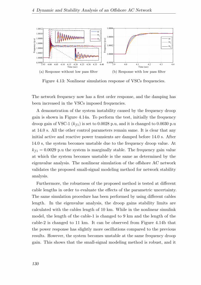
4 Dynamic and Stability Analysis of an Offshore AC Network

3.95 4.00 4.05 4.10 4.15 4.20 4.25 4.30 4.350.9998

1.0000

1.0002

1.0004

1.0006

1.0008

1.0010

1.0012

Time (sec)

Fre

quen

cy (

p.u

)1

2

4.40

(a) Response without low pass filter

3.9 4.0 4.1 4.2 4.3 4.40.9998

1.0000

1.0002

1.0004

1.0006

Time (sec)

Fre

quen

cy (

p.u

)

1

2

(b) Response with low pass filter

Figure 4.13: Nonlinear simulation response of VSCs frequencies.

The network frequency now has a first order response, and the damping has

been increased in the VSCs imposed frequencies.

A demonstration of the system instability caused by the frequency droop

gain is shown in Figure 4.14a. To perform the test, initially the frequency

droop gain of VSC-1 (kf1) is set to 0.0028 p.u, and it is changed to 0.0030 p.u

at 14.0 s. All the other control parameters remain same. It is clear that any

initial active and reactive power transients are damped before 14.0 s. After

14.0 s, the system becomes unstable due to the frequency droop value. At

kf1 = 0.0029 p.u the system is marginally stable. The frequency gain value

at which the system becomes unstable is the same as determined by the

eigenvalue analysis. The nonlinear simulation of the offshore AC network

validates the proposed small-signal modeling method for network stability

analysis.

Furthermore, the robustness of the proposed method is tested at different

cable lengths in order to evaluate the effects of the parametric uncertainty.

The same simulation procedure has been performed by using different cables

length. In the eigenvalue analysis, the droop gains stability limits are

calculated with the cables length of 10 km. While in the nonlinear simulink

model, the length of the cable-1 is changed to 9 km and the length of the

cable-2 is changed to 11 km. It can be observed from Figure 4.14b that

the power response has slightly more oscillations compared to the previous

results. However, the system becomes unstable at the same frequency droop

gain. This shows that the small-signal modeling method is robust, and it

130

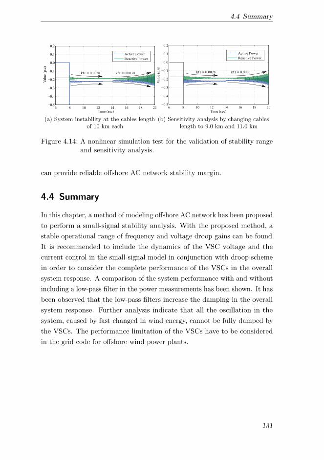
4.4 Summary

6 8 10 12 14 16 18 200.5

0.4

0.3

0.2

0.1

0.0

0.1

0.2

Time (sec)

Val

ue

(p.u

)

Active Power

Reactive Power

kf1 = 0.0028 kf1 = 0.0030

(a) System instability at the cables lengthof 10 km each

6 8 10 12 14 16 18 200.5

0.4

0.3

0.2

0.1

0.0

0.1

0.2

Time (sec)

Val

ue

(p.u

)

Active Power

Reactive Power

kf1 = 0.0028 kf1 = 0.0030

(b) Sensitivity analysis by changing cableslength to 9.0 km and 11.0 km

Figure 4.14: A nonlinear simulation test for the validation of stability rangeand sensitivity analysis.

can provide reliable offshore AC network stability margin.

4.4 Summary

In this chapter, a method of modeling offshore AC network has been proposed

to perform a small-signal stability analysis. With the proposed method, a

stable operational range of frequency and voltage droop gains can be found.

It is recommended to include the dynamics of the VSC voltage and the

current control in the small-signal model in conjunction with droop scheme

in order to consider the complete performance of the VSCs in the overall

system response. A comparison of the system performance with and without

including a low-pass filter in the power measurements has been shown. It has

been observed that the low-pass filters increase the damping in the overall

system response. Further analysis indicate that all the oscillation in the

system, caused by fast changed in wind energy, cannot be fully damped by

the VSCs. The performance limitation of the VSCs have to be considered

in the grid code for offshore wind power plants.

131

132

5 Short Circuit Analysis of an

Offshore AC Network

This chapter presents the short circuit analysis of an offshore AC network

that interconnects the offshore wind power plants with different onshore

grids using VSC-HVDC transmission system. The short circuit control

system is presented for the wind turbines, onshore and offshore VSCs. The

chapter presents a method to calculate the control limits of VSCs considering

operational capability. Furthermore, the short circuit analysis of a network

has been performed to propose the suitable control scheme. In order to verify

the proposed short circuit control scheme, three phase symmetric faults are

applied on a wind turbine busbar, offshore HVAC busbar, at the offshore AC

cable that interconnects the VSC-HVDC systems, and at the onshore grid.

Additionally, a frequency coordination control scheme is proposed between

wind power generation and offshore VSCs of HVDC systems without using

communication signal. The methodology and control system are validated

by performing a nonlinear simulation5,6.

5.1 Introduction

An offshore grid has importance in the integration of the future large

offshore wind power plants with the onshore grids [111]. The concept

5This chapter is based on the following publications:M. Raza, M. Aragues-Penalba, and O. Gomis-Bellmunt, “Short circuit analysis of anoffshore AC network having multiple VSCs imposing frequency” International Journalof Electrical Power and Energy Systems, Elseiver (peer-reviewed).

6M. Raza and O. Gomis-Bellmunt, “Control design strategy to enhance the fault ridethrough capability of VSC-HVDC transmission system interconnecting offshore windpower plant”, in EWEA Annual Conference and Exhibition 2015, (Paris, France), nov2015.

133

5 Short Circuit Analysis of an Offshore AC Network

of the offshore grid control principle has been presented in the previous

chapters. The control principle covers the operation of the network with

respect of steady state behavior, dynamic response, and small signal stability.

The complete successful operation of an offshore grid further requires that

the wind generation units and offshore VSCs should continue operating

during fault for short period of time, and they must continue to function

after isolation of faulted area [112]. The grid integration requirements are

usually provided by transmission operators in their grid codes [47]. The

fault ride through (FRT) capability is required even at very low fault voltage.

For the onshore grid connection, the grid code requirements are fulfilled

by onshore converters of VSC-HVDC transmission system at the point of

common coupling (PCC) [113]. During low voltage ride through or fault,

it is recommended to inject the reactive current in order to support the

onshore grid voltage. However during recovery period, this reactive current

must be removed as fast as possible, and the rate of active power recovery

should also be high to ensure system stability [83].

In the network such as illustrated in Figure 5.1, VSCs of HVDC transmis-

sion system decouple the offshore grid from the mainland grid which makes

offshore grid vulnerable to dynamic voltage events due to low short circuit

power in the network [114]. The short circuit power in the offshore network is

limited by the maximum rated power of the HVDC transmission system and

wind turbines. The offshore network formation by interconnecting several

offshore wind power plants may increase the short circuit current level in the

network compare to a single wind power plant connection with an onshore

grid. However, it is important that the offshore VSCs of HVDC systems

must ensure the voltage stability during fault and post fault states. In the

event of fault, the VSC operation is switched from control voltage source

to current source once current limit reaches. In this situation, the network

complex voltage at the VSC controlling busbar appears according to the

equivalent fault impedance and the VSC current [83]. Depending on the VSC

current angle infeed, the fault voltage angle could deviate significantly from

its pre-fault state. The large angle deviation can cause instability during

recovery period [82]. This requires a suitable control scheme to improve the

voltage phase angle during fault close to the level of pre-fault state. This

134

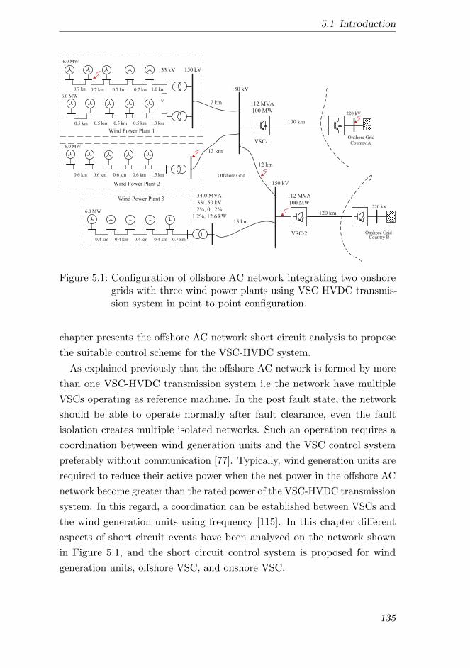
5.1 Introduction

7 km

13 km

1.0 km0.7 km0.7 km

15 km

12 km

100 km

120 km

0.6 km 0.6 km 1.5 km

150 kV

34.0 MVA

33/150 kV

2%, 0.12%

1.2%, 12.6 kW

6.0 MW

0.7 km

0.6 km

0.4 km 0.4 km 0.7 km0.4 km

6.0 MW

6.0 MW

33 kV

0.5 km 0.5 km0.5 km

6.0 MW

1.3 km

112 MVA

100 MW

112 MVA

100 MW

VSC-1

VSC-2

150 kV

0.7 km

0.5 km

0.6 km

0.4 km

150 kV

Wind Power Plant 1

Wind Power Plant 2

Wind Power Plant 3

220 kV

220 kV

Country A

Country B

Offshore Grid

Onshore Grid

Onshore Grid

Figure 5.1: Configuration of offshore AC network integrating two onshoregrids with three wind power plants using VSC HVDC transmis-sion system in point to point configuration.

chapter presents the offshore AC network short circuit analysis to propose

the suitable control scheme for the VSC-HVDC system.

As explained previously that the offshore AC network is formed by more

than one VSC-HVDC transmission system i.e the network have multiple

VSCs operating as reference machine. In the post fault state, the network

should be able to operate normally after fault clearance, even the fault

isolation creates multiple isolated networks. Such an operation requires a

coordination between wind generation units and the VSC control system

preferably without communication [77]. Typically, wind generation units are

required to reduce their active power when the net power in the offshore AC

network become greater than the rated power of the VSC-HVDC transmission

system. In this regard, a coordination can be established between VSCs and

the wind generation units using frequency [115]. In this chapter different

aspects of short circuit events have been analyzed on the network shown

in Figure 5.1, and the short circuit control system is proposed for wind

generation units, offshore VSC, and onshore VSC.

135

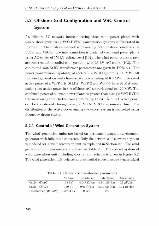
5 Short Circuit Analysis of an Offshore AC Network

5.2 Offshore Grid Configuration and VSC Control

System

An offshore AC network interconnecting three wind power plants with

two onshore grids using VSC-HVDC transmission systems is illustrated in

Figure 5.1. The offshore network is formed by both offshore converters i.e

VSC-1 and VSC-2. The interconnection is made between wind power plants

using AC cables of 150 kV voltage level [102]. The wind power plants arrays

are constructed in radial configuration with 33 kV AC cables [103]. The

cables and 150/33 kV transformer parameters are given in Table 5.1. The

power transmission capability of each VSC-HVDC system is 100 MW. All

the wind generation units have active power rating of 6.0 MW. The rated

active power of a WPP-1 is 60 MW, WPP-2 and WPP-3 have 30 MW each,

making net active power in the offshore AC network equal to 120 MW. The

combined power of all wind power plants is greater than a single VSC-HVDC

transmission system. In this configuration, up to 83.3 % of net active power

can be transferred through a signal VSC-HVDC transmission line. The

distribution of the active power among the export system is controlled using

frequency droop control.

5.2.1 Control of Wind Generation System

The wind generation units are based on permanent magnet synchronous

generator with fully rated converter. Only the network side converter system

is modeled for a wind generation unit as explained in Section 2.5. The wind

generation unit parameters are given in Table 2.3. The control system of

wind generation unit including short circuit scheme is given in Figure 5.2.

The wind generation unit behaves as a controlled current source synchronized

Table 5.1: Cables and transformer parameters

Voltage Resistance Inductance Capacitance

Cable (MVAC) 33 kV 0.047 Ω/km 0.34 mH/km 0.3 µF/km

Cable (HVAC) 150 kV 0.06 Ω/km 0.44 mH/km 0.14 µF/km

Transformer (HV-MV) 150/33 kV 0.12% 2% -

136

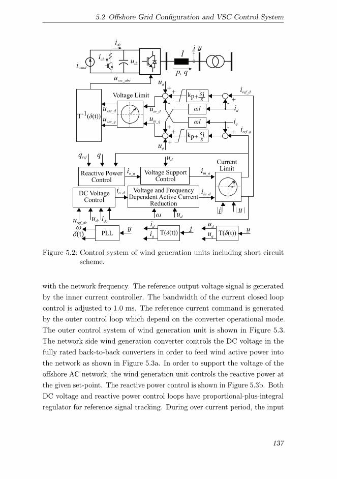
5.2 Offshore Grid Configuration and VSC Control System

iwind

udc

i ul

idc

ich

kp+kis

kp+kis

+

-+

+-

+

-

++

+

T-1( (t))

id

iq

ud

uq

T( (t))

Voltage Limit

l

l

T( (t))

CurrentLimit

Voltage and FrequencyDependent Active Current

Reduction

iref_d

iref_q

iin_d

iin_q

DC VoltageControl

Voltage SupportControl

Reactive PowerControl

uref_dc

qref

PLL

ud

uq

uid

iq

iu

p, q

q

udc

uvsc_abc

io_q

io_d

uin_d

uin_q

uvsc_d

uvsc_q

ud

ud

| u |

idc

(t)

Figure 5.2: Control system of wind generation units including short circuitscheme.

with the network frequency. The reference output voltage signal is generated

by the inner current controller. The bandwidth of the current closed loop

control is adjusted to 1.0 ms. The reference current command is generated

by the outer control loop which depend on the converter operational mode.

The outer control system of wind generation unit is shown in Figure 5.3.

The network side wind generation converter controls the DC voltage in the

fully rated back-to-back converters in order to feed wind active power into

the network as shown in Figure 5.3a. In order to support the voltage of the

offshore AC network, the wind generation unit controls the reactive power at

the given set-point. The reactive power control is shown in Figure 5.3b. Both

DC voltage and reactive power control loops have proportional-plus-integral

regulator for reference signal tracking. During over current period, the input

137

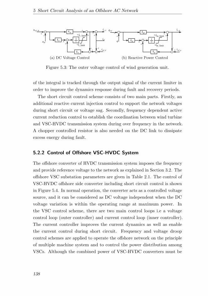
5 Short Circuit Analysis of an Offshore AC Network

kvp

udc

io_d

+

idc

-

s1kvi

+

+

kvi

++

iref_d-+

+-

uref_dc

+-

+ir_limit

-ir_limit

(a) DC Voltage Control

kqp

q

io_q

s1kqi

++

kqi

++

iref_q-+

+

-

qref

+im_limit

-im_limit

(b) Reactive Power Control

Figure 5.3: The outer voltage control of wind generation unit.

of the integral is tracked through the output signal of the current limiter in

order to improve the dynamics response during fault and recovery periods.

The short circuit control scheme consists of two main parts. Firstly, an

additional reactive current injection control to support the network voltages

during short circuit or voltage sag. Secondly, frequency dependent active

current reduction control to establish the coordination between wind turbine

and VSC-HVDC transmission system during over frequency in the network.

A chopper controlled resistor is also needed on the DC link to dissipate

excess energy during fault.

5.2.2 Control of Offshore VSC-HVDC System

The offshore converter of HVDC transmission system imposes the frequency

and provide reference voltage to the network as explained in Section 3.2. The

offshore VSC substation parameters are given in Table 2.1. The control of

VSC-HVDC offshore side converter including short circuit control is shown

in Figure 5.4. In normal operation, the converter acts as a controlled voltage

source, and it can be considered as DC voltage independent when the DC

voltage variation is within the operating range at maximum power. In

the VSC control scheme, there are two main control loops i.e a voltage

control loop (outer controller) and current control loop (inner controller).

The current controller improves the current dynamics as well as enable

the current control during short circuit. Frequency and voltage droop

control schemes are applied to operate the offshore network on the principle

of multiple machine system and to control the power distribution among

VSCs. Although the combined power of VSC-HVDC converters must be

138

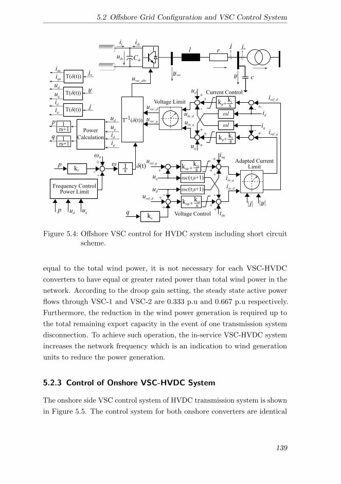
5.2 Offshore Grid Configuration and VSC Control System

i

udc

l r

c

Cdc

il idc

kp+ki

s

kop +koi

s

c( is+1)

+

- +

+-

-+

+-

+

-

++

+

+

++

++

-

T-1( (t))

in

id

iq

idn

inq

ud

uq

ud

uq

uref_d

uref_q

ku

+

1skf

+

-

0

p

q

T( (t))

uduqidiq

q

p

Power

Calculation

uvsc_abc

Voltage Limit

Adapted CurrentLimit

idniqn

Frequency ControlPower Limit

-

p

l

l

T( (t))

T( (t))

iref_d

iref_q

uvsc uin

u

i

uduqidiq

uin_duin_q

uvsc_d

uvsc_q

iin_d

iin_q

Current Control

c( is+1)

ud uq

|u|

Voltage Control

|i|

s+11

s+11 kp+

ki

s

kop +koi

s

(t)

Figure 5.4: Offshore VSC control for HVDC system including short circuitscheme.

equal to the total wind power, it is not necessary for each VSC-HVDC

converters to have equal or greater rated power than total wind power in the

network. According to the droop gain setting, the steady state active power

flows through VSC-1 and VSC-2 are 0.333 p.u and 0.667 p.u respectively.

Furthermore, the reduction in the wind power generation is required up to

the total remaining export capacity in the event of one transmission system

disconnection. To achieve such operation, the in-service VSC-HVDC system

increases the network frequency which is an indication to wind generation

units to reduce the power generation.

5.2.3 Control of Onshore VSC-HVDC System

The onshore side VSC control system of HVDC transmission system is shown

in Figure 5.5. The control system for both onshore converters are identical

139

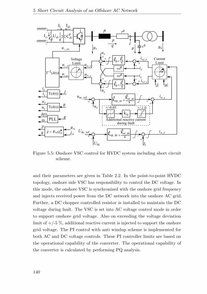
5 Short Circuit Analysis of an Offshore AC Network

i

Udc

lg rg

Cdc

Il Idc

uv u un

kp+kis

kp+kis

+

-+

+-

+

-

++

+

T-1( (t))

id

iq

ud

uq

l

l

iref_d

iref_q

uv_d

uv_q

uv_abc

T( (t))u

uduq

T( (t))i

idiq

g

koi_dc

skop_dc +

Udc_ref

Udc Il

++

(t)PLL

u

+

p

q

idq

udqp

q udq idq=s gg

gg

gg

g

g

cg

ud

uac_ref koi_ac

skop_ac +g

g

--

-

uin_d

uin_q

VoltageLimit

CurrentLimit

kiq

+/-0.05

Additional reactive currentduring fault

+/-1.0

++

|u||i|

Ich

iin_q

iin_d

Figure 5.5: Onshore VSC control for HVDC system including short circuitscheme.

and their parameters are given in Table 2.2. In the point-to-point HVDC

topology, onshore side VSC has responsibility to control the DC voltage. In

this mode, the onshore VSC is synchronized with the onshore grid frequency

and injects received power from the DC network into the onshore AC grid.

Further, a DC chopper controlled resistor is installed to maintain the DC

voltage during fault. The VSC is set into AC voltage control mode in order

to support onshore grid voltage. Also on exceeding the voltage deviation

limit of +/-5 %, additional reactive current is injected to support the onshore

grid voltage. The PI control with anti windup scheme is implemented for

both AC and DC voltage controls. These PI controller limits are based on

the operational capability of the converter. The operational capability of

the converter is calculated by performing PQ analysis.

140

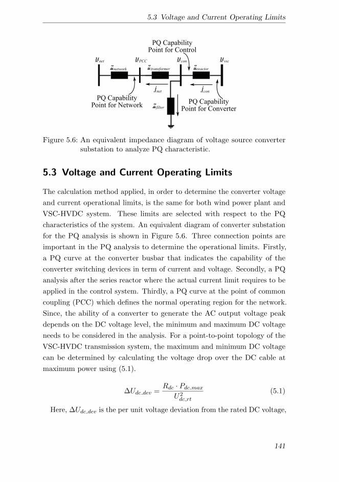
5.3 Voltage and Current Operating Limits

icon

uvsczreactor

zfilter

ztransformerznetwork

uconuPCCunet

inet

PQ CapabilityPoint for Converter

PQ CapabilityPoint for Control

PQ CapabilityPoint for Network

Figure 5.6: An equivalent impedance diagram of voltage source convertersubstation to analyze PQ characteristic.

5.3 Voltage and Current Operating Limits

The calculation method applied, in order to determine the converter voltage

and current operational limits, is the same for both wind power plant and

VSC-HVDC system. These limits are selected with respect to the PQ

characteristics of the system. An equivalent diagram of converter substation

for the PQ analysis is shown in Figure 5.6. Three connection points are

important in the PQ analysis to determine the operational limits. Firstly,

a PQ curve at the converter busbar that indicates the capability of the

converter switching devices in term of current and voltage. Secondly, a PQ

analysis after the series reactor where the actual current limit requires to be

applied in the control system. Thirdly, a PQ curve at the point of common

coupling (PCC) which defines the normal operating region for the network.

Since, the ability of a converter to generate the AC output voltage peak

depends on the DC voltage level, the minimum and maximum DC voltage

needs to be considered in the analysis. For a point-to-point topology of the

VSC-HVDC transmission system, the maximum and minimum DC voltage

can be determined by calculating the voltage drop over the DC cable at

maximum power using (5.1).

∆Udc dev =Rdc · Pdc max

U2dc rt

(5.1)

Here, ∆Udc dev is the per unit voltage deviation from the rated DC voltage,

141

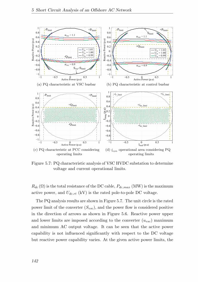
5 Short Circuit Analysis of an Offshore AC Network

1 0.5 0 0.5 11

0.8

0.6

0.4

0.2

0

0.2

0.4

0.6

0.8

1

Active Power (p.u)

Rea

ctiv

e P

ow

er (

p.u

)

Udc = 0.99Udc = 1.00Udc = 1.01

+Plimit-Plimit

-Qlimit

uvsc = 0.9

uvsc = 1.1

Svsc=Slimit

(a) PQ characteristic at VSC busbar

1 0.5 0 0.5 11

0.8

0.6

0.4

0.2

0

0.2

0.4

0.6

0.8

1

Active Power (p.u)

Rea

ctiv

e P

ow

er (

p.u

)

Udc = 0.99Udc = 1.00Udc = 1.01

+Plimit-Plimit

+Qlimit

uvsc = 0.9

uvsc = 1.1

Slimit

(b) PQ characteristic at control busbar

1 0.5 0 0.5 11

0.8

0.6

0.4

0.2

0

0.2

0.4

0.6

0.8

1

Active Power (p.u)

Rea

ctiv

e P

ow

er (

p.u

)

-Plimit +Plimit

+Qlimit

-Qlimit

(c) PQ characteristic at PCC consideringoperating limits

1 0.5 0 0.5 11

0.8

0.6

0.4

0.2

0

0.2

0.4

0.6

0.8

1

I im

ag (

p.u

)

Ireal (p.u)

+ir_limit-ir_limit

+im_limit

-im_limit

(d) icon operational area considering PQoperating limits

Figure 5.7: PQ characteristic analysis of VSC HVDC substation to determinevoltage and current operational limits.

Rdc (Ω) is the total resistance of the DC cable, Pdc max (MW) is the maximum

active power, and Udc rt (kV) is the rated pole-to-pole DC voltage.

The PQ analysis results are shown in Figure 5.7. The unit circle is the rated

power limit of the converter (Svsc), and the power flow is considered positive

in the direction of arrows as shown in Figure 5.6. Reactive power upper

and lower limits are imposed according to the converter (uvsc) maximum

and minimum AC output voltage. It can be seen that the active power

capability is not influenced significantly with respect to the DC voltage

but reactive power capability varies. At the given active power limits, the

142

5.4 Short Circuit Analysis of an Offshore Grid

inductive reactive power (−Qlimit) is determined at minimum AC voltage

and at maximum DC voltage, as illustrated in Figure 5.7a. Care must be

taken while selecting reactive power limits to not to violate all limits on

PQ capability curve at both converter and control busbar. The maximum

capacitive reactive power limit (Qlimit) is set by PQ curves at control busbar

at maximum AC and at minimum DC voltage as illustrated in Figure 5.7b. It

can be noticed that capacitive reactive power limit is further reduced due to

losses in the reactor. The operating region at the point of common coupling

considering active and reactive power limits is shown in Figure 5.7c. Further,

maximum steady state current limit can be determined from Figure 5.7d.

Also, the maximum required modulation index can be calculated using (5.2).

m =uac maxUdc min

· 2up rtUdc rt

(5.2)

Here, uac max (p.u) is the maximum AC output voltage, Udc min (p.u) is

the minimum DC voltage for normal operation, up rt (kV) is the rated AC

output voltage, and Udc rt (kV) is the rated DC voltage.

5.4 Short Circuit Analysis of an Offshore Grid

The principle of VSC short circuit control can be understood by performing

circuit theory analysis on a simplified network given in Figure 5.8. The wind

power plants fault current is represented by the net current (i7) injecting at

the fault busbar (u7). The VSCs behave as controlled voltage sources in the

pre-fault state. However, these converters are required to be operated as

control current sources during fault period and inject short circuit current

up to their maximum capability. The impact of the short circuit current

on the network voltages during fault can be analyzed by defining the net

current infeed (ivsc) of the VSCs and the wind power plant current at

the cable-1 ends as redrawn in Figure 5.8b. Here, zfault is the parallel

combination of the fault impedance and the cable capacitive impedance

(zc1 f ). In parallel combination, the fault impedance is dominant due to

smaller in value therefore only the fault impedance is shown in the equivalent

network diagram. The bus voltages as a function of VSC and wind power

143

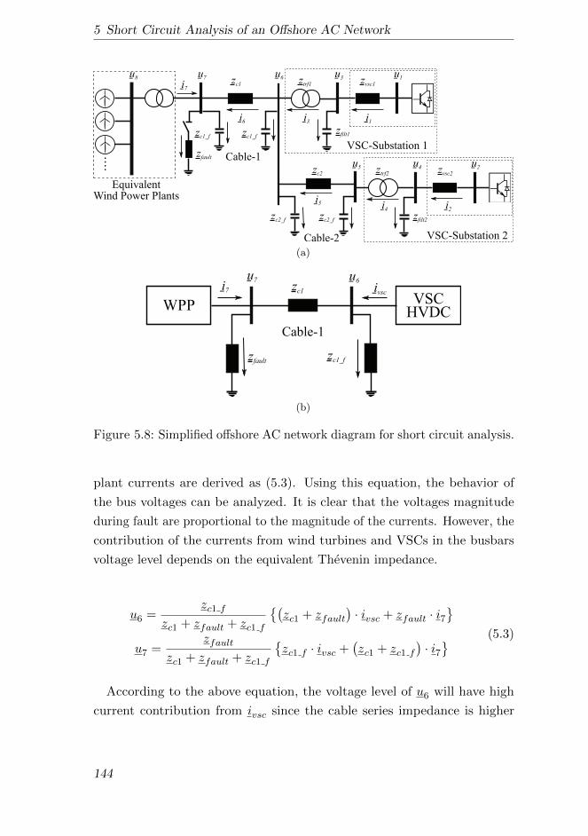
5 Short Circuit Analysis of an Offshore AC Network

u6 zvsc1

zfilt1

ztrf1zc1u1

u2

u3

i1

zfault

i7

zc1_fzc1_f

i2

u5

i5

u7

zvsc2

zfilt2

ztrf2u4

i3

u8

i4

i6

zc2

zc2_fzc2_f

VSC-Substation 1

VSC-Substation 2

EquivalentWind Power Plants

Cable-1

Cable-2

(a)

u6

zc1_f

zc1u7

ivsc

zfault

VSCHVDC

WPP

i7

Cable-1

(b)

Figure 5.8: Simplified offshore AC network diagram for short circuit analysis.

plant currents are derived as (5.3). Using this equation, the behavior of

the bus voltages can be analyzed. It is clear that the voltages magnitude

during fault are proportional to the magnitude of the currents. However, the

contribution of the currents from wind turbines and VSCs in the busbars

voltage level depends on the equivalent Thevenin impedance.

u6 =zc1 f

zc1 + zfault + zc1 f

(zc1 + zfault

)· ivsc + zfault · i7

u7 =

zfaultzc1 + zfault + zc1 f

zc1 f · ivsc +

(zc1 + zc1 f

)· i7 (5.3)

According to the above equation, the voltage level of u6 will have high

current contribution from ivsc since the cable series impedance is higher

144

5.4 Short Circuit Analysis of an Offshore Grid

0.05

0.1

0.15

30

210

60

240

90

270

120

300

150

330

180 0

u6u7

zfault

(a)

1

2

3

4

30

210

60

240

90

270

120

300

150

330

180 0

zfault = 0

zfault

6

(b)

Figure 5.9: Effect of fault impedance magnitude on busbar voltages.

than the fault impedance i.e(zc1 + zfault

)> zfault. Similarly, the voltage

level of u7 will be improved mainly by wind turbine current infeed. Apart

of the current, the equivalent impedances also have high impact on the

busbars voltage. The fault impedance introduces the voltage phase angle

shift or phase angle jump due to difference in the equivalent impedance in

fault and pre-fault states [116]. The power electronic devices are sensitive

to phase angle jump which lead to their mal-operation and cause instability

in the network. During fault, the busbar voltage phase angle difference

needs to be analyzed with respect to its pre-fault value as well as from other

voltage source bus phase angle. In order to do so, the effect of the fault

impedance on the voltage phase angle is analyzed by phasor diagram as

shown in Figure 5.9. The fault is considered as three phase resistive. In

the results, the wind power plants are not injecting any current i.e i7 = 0.0,

and the VSC injects rated current i.e ivsc = 1.0∠0.0 deg. Note that the

(5.3) represents the steady state voltage values during fault. Further, the

converters are operating as controlled current sources during short circuit

therefore its current can be taken as the reference vector on the complex

plane. The voltage, current and impedance variables are expressed in polar

coordinate to simply the notation as:

145

5 Short Circuit Analysis of an Offshore AC Network

u6 = u6ejδ6

u7 = u7ejδ7

i7 = i7ejψ7

ivsc = ivscejψvsc

zfault = zfejθf

zc1 = zcejθc

zc1 f = zcfejθcf

(5.4)

Typically, pre-fault voltage phase angle is near 0.0 deg from the reference

bus considering no phase shifting transformer included. Figure 5.9a illustrate

that the phase angle of δ6 changes significant with the reduction in the

magnitude of the fault impedance. Also, the phase difference of both busbar

i.e δ6 − δ7 increases proportionally. These large angle deviations can cause

instability during fault and recovery period. Further, δ7 is not changed from

its pre-fault value since the wind turbines current is zero and the voltage

level is due to converter current. Note that zf only influences u7 but not δ7.

To quantify the voltage angle deviation as function of equivalent impedance,

a complex voltage ratio η6

is defined for busbar 6 as given by (5.5). Note

that in the equation i7 = 0.0 p.u.

η6

=u6

u06

=1 +

zfzcej(θf−θc)

1 +zfzxej(θf−θx)

(5.5)

Here, zx = zc1 + zc1 f . Also, u06 refers to the voltage at the busbar 6 when

the fault impedance is zero. Figure 5.9b illustrate the relative deviation

in η6

with respect to voltage when the fault impedance is zero. On the

complex plane, the reference vector is u06 i.e 1.0∠0.0 deg. The impedance

of the cable capacitance is high relative to the fault impedance therefore

denominator in (5.5) is constant i.e 1 >> zf/zx. Thus, the voltage angle

deviation mainly occurs due to the cable series impedance angle which is

inductive i.e θc ≈ 90 deg. With the increase in the zf , the voltage at busbar 6

increases since the condition 1 < zf/zc is applied. In the plot, θf is constant

at the value of 0.0 deg. This has demonstrated that the phase angle jump is

the function of the equivalent fault impedance which varies according to the

146

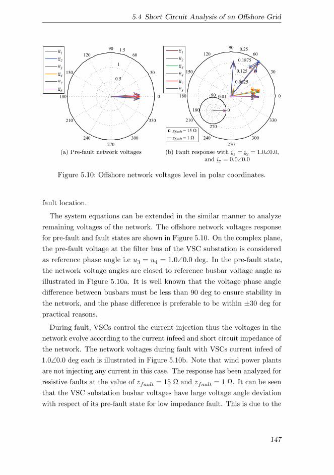
5.4 Short Circuit Analysis of an Offshore Grid

0.5

1

1.5

30

210

60

240

90

270

120

300

150

330

180 0

u1

u2

u3

u4

u7

u8

(a) Pre-fault network voltages

0.0625

0.125

0.1875

0.25

30

210

60

240

90

270

120

300

150

330

180 0

u1

u2

u3

u4

u7

u8

0.01

0

90

270

180

zfault = 15

zfault = 1

(b) Fault response with i1 = i2 = 1.0∠0.0,and i7 = 0.0∠0.0

Figure 5.10: Offshore network voltages level in polar coordinates.

fault location.

The system equations can be extended in the similar manner to analyze

remaining voltages of the network. The offshore network voltages response

for pre-fault and fault states are shown in Figure 5.10. On the complex plane,

the pre-fault voltage at the filter bus of the VSC substation is considered

as reference phase angle i.e u3 = u4 = 1.0∠0.0 deg. In the pre-fault state,

the network voltage angles are closed to reference busbar voltage angle as

illustrated in Figure 5.10a. It is well known that the voltage phase angle

difference between busbars must be less than 90 deg to ensure stability in

the network, and the phase difference is preferable to be within ±30 deg for

practical reasons.

During fault, VSCs control the current injection thus the voltages in the

network evolve according to the current infeed and short circuit impedance of

the network. The network voltages during fault with VSCs current infeed of

1.0∠0.0 deg each is illustrated in Figure 5.10b. Note that wind power plants

are not injecting any current in this case. The response has been analyzed for

resistive faults at the value of zfault = 15 Ω and zfault = 1 Ω. It can be seen

that the VSC substation busbar voltages have large voltage angle deviation

with respect of its pre-fault state for low impedance fault. This is due to the

147

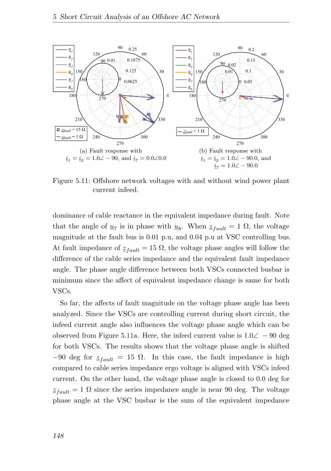
5 Short Circuit Analysis of an Offshore AC Network

0.0625

0.125

0.1875

0.25

30

210

60

240

90

270

120

300

150

330

180 0

u1

u2

u3

u4

u7

u8

0.01

0

90

180

270

zfault = 15

zfault = 1

(a) Fault response withi1 = i2 = 1.0∠− 90, and i7 = 0.0∠0.0

0.05

0.1

0.15

0.2

30

210

60

240

90

270

120

300

150

330

180 0

u1

u2

u3

u4

u7

u8

0.01

0.02

0

90

180

270

zfault = 1

(b) Fault response withi1 = i2 = 1.0∠− 90.0, and

i7 = 1.0∠− 90.0

Figure 5.11: Offshore network voltages with and without wind power plantcurrent infeed.

dominance of cable reactance in the equivalent impedance during fault. Note

that the angle of u7 is in phase with u8. When zfault = 1 Ω, the voltage

magnitude at the fault bus is 0.01 p.u, and 0.04 p.u at VSC controlling bus.

At fault impedance of zfault = 15 Ω, the voltage phase angles will follow the

difference of the cable series impedance and the equivalent fault impedance

angle. The phase angle difference between both VSCs connected busbar is

minimum since the affect of equivalent impedance change is same for both

VSCs.

So far, the affects of fault magnitude on the voltage phase angle has been

analyzed. Since the VSCs are controlling current during short circuit, the

infeed current angle also influences the voltage phase angle which can be

observed from Figure 5.11a. Here, the infeed current value is 1.0∠ − 90 deg

for both VSCs. The results shows that the voltage phase angle is shifted

−90 deg for zfault = 15 Ω. In this case, the fault impedance is high

compared to cable series impedance ergo voltage is aligned with VSCs infeed

current. On the other hand, the voltage phase angle is closed to 0.0 deg for

zfault = 1 Ω since the series impedance angle is near 90 deg. The voltage

phase angle at the VSC busbar is the sum of the equivalent impedance

148

5.5 Short Circuit and Frequency Coordinated Control System

angle and VSC current angle. It can be concluded that the VSC current

is required to be controlled according to the equivalent impedance as seen

from its controlling busbar (filter bus) in order to keep its busbar voltage

angle near to pre-fault state. Further, the magnitude of the VSC substation

voltages are not affected by the current angle rather they are proportional

to the magnitude of the current. Thus, the VSCs must inject current of

maximum magnitude in order to maximize the voltages during fault.

As it has been observed that the voltages at the wind power plants busbar

(u8) mainly depends on the fault busbar voltages. The further improvement

in the voltage at the busbar 8 can be done by wind power plant current

injections as shown in Figure 5.11b. It is clear that the current injection with

the angle −90 deg by the wind power plants improves both the magnitude

and angle of u8. The fault bus voltage can be calculated using (5.6).

u7 = zfault · (i7 + i6) where i6 ≈ i1 + i2 (5.6)

5.5 Short Circuit and Frequency Coordinated Control

System

There are two aspects of large signal disturbance that need to be considered

in the control system for an offshore AC network. Firstly, a short circuit

in the network leads to low voltages. In this case, converters behave as a

controlled current source injecting maximum current. After fault isolation,

the network must be restored as fast as possible and even create more than

one isolated network if needed, such as in case of fault on interconnected

cable (12 km) as shown in Figure 5.1. Secondly, the availability of more

power in the offshore AC network than the export capacity. Such situation

may appear when one VSC-HVDC transmission system is disconnected and

the remaining in-operation transmission system has less export capacity

than net power available in the network. In this case, the network frequency

needs to be increased by the VSC-HVDC system to indicate wind generation

systems to reduce their power generation up to the limit of export capacity.

In this section, the control scheme is designed with respect of both scenarios.

149

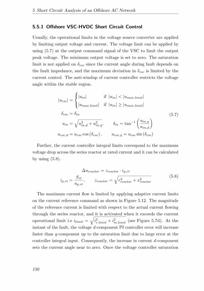
5 Short Circuit Analysis of an Offshore AC Network

5.5.1 Offshore VSC-HVDC Short Circuit Control

Usually, the operational limits in the voltage source converter are applied

by limiting output voltage and current. The voltage limit can be applied by

using (5.7) at the output command signal of the VSC to limit the output

peak voltage. The minimum output voltage is set to zero. The saturation

limit is not applied on δvsc since the current angle during fault depends on

the fault impedance, and the maximum deviation in δvsc is limited by the

current control. The anti-windup of current controller restricts the voltage

angle within the stable region.

|uvsc| =

|uin| if |uin| < |umax limit|

|umax limit| if |uin| ≥ |umax limit|

δvsc = δin

uin =√u2in d + u2

in q, δin = tan−1

(uin quin d

)uvsc d = uvsc cos (δvsc) , uvsc q = uvsc sin (δvsc)

(5.7)

Further, the current controller integral limits correspond to the maximum

voltage drop across the series reactor at rated current and it can be calculated

by using (5.8).

∆ureactor = zreactor · ip rt

ip rt =Srtup rt

, zreactor =√r2reactor + x2

reactor

(5.8)

The maximum current flow is limited by applying adaptive current limits

on the current reference command as shown in Figure 5.12. The magnitude

of the reference current is limited with respect to the actual current flowing

through the series reactor, and it is activated when it exceeds the current

operational limit i.e ilimit =√i2r limit + i2m limit (see Figure 5.7d). At the

instant of the fault, the voltage d -component PI controller error will increase

faster than q-component up to the saturation limit due to large error at the

controller integral input. Consequently, the increase in current d -component

sets the current angle near to zero. Once the voltage controller saturation

150

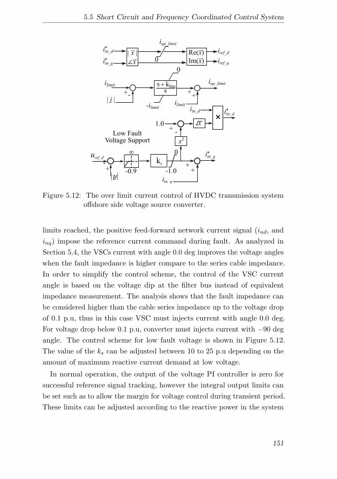
5.5 Short Circuit and Frequency Coordinated Control System

iin_q

iin_d iref_d

iref_q

| x | Re(x)

Im(x)

iup_limit

s

0

++

iup_limit

+-

ilimit

| i |

x 0

ks

-0.9+-

uref_d

|u|

++

iin_q

iin_q

iin_diin_d

x2

x+

1.0

0

-1.0

-Low FaultVoltage Support

-ilimitilimit

s + klim

Figure 5.12: The over limit current control of HVDC transmission systemoffshore side voltage source converter.

limits reached, the positive feed-forward network current signal (ind, and

inq) impose the reference current command during fault. As analyzed in

Section 5.4, the VSCs current with angle 0.0 deg improves the voltage angles

when the fault impedance is higher compare to the series cable impedance.

In order to simplify the control scheme, the control of the VSC current

angle is based on the voltage dip at the filter bus instead of equivalent

impedance measurement. The analysis shows that the fault impedance can

be considered higher than the cable series impedance up to the voltage drop

of 0.1 p.u, thus in this case VSC must injects current with angle 0.0 deg.

For voltage drop below 0.1 p.u, converter must injects current with −90 deg

angle. The control scheme for low fault voltage is shown in Figure 5.12.

The value of the ks can be adjusted between 10 to 25 p.u depending on the

amount of maximum reactive current demand at low voltage.

In normal operation, the output of the voltage PI controller is zero for

successful reference signal tracking, however the integral output limits can

be set such as to allow the margin for voltage control during transient period.

These limits can be adjusted according to the reactive power in the system

151

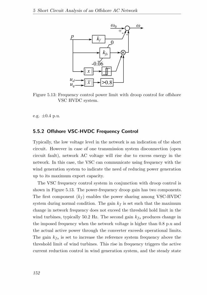
5 Short Circuit Analysis of an Offshore AC Network

0

-0.06

| x |

0

kfp

+- -

| x |uduq

>0.8

kfs

Figure 5.13: Frequency control power limit with droop control for offshoreVSC HVDC system.

e.g. ±0.4 p.u.

5.5.2 Offshore VSC-HVDC Frequency Control

Typically, the low voltage level in the network is an indication of the short

circuit. However in case of one transmission system disconnection (open

circuit fault), network AC voltage will rise due to excess energy in the

network. In this case, the VSC can communicate using frequency with the

wind generation system to indicate the need of reducing power generation

up to its maximum export capacity.

The VSC frequency control system in conjunction with droop control is

shown in Figure 5.13. The power-frequency droop gain has two components.

The first component (kf ) enables the power sharing among VSC-HVDC

system during normal condition. The gain kf is set such that the maximum

change in network frequency does not exceed the threshold hold limit in the

wind turbines, typically 50.2 Hz. The second gain kfs produces change in

the imposed frequency when the network voltage is higher than 0.8 p.u and

the actual active power through the converter exceeds operational limits.

The gain kfs is set to increase the reference system frequency above the

threshold limit of wind turbines. This rise in frequency triggers the active

current reduction control in wind generation system, and the steady state

152

5.5 Short Circuit and Frequency Coordinated Control System

-

ud

+

uo

-0.05

io_q iin_q

kwq

0.05

+

+

Figure 5.14: Voltage support control scheme of wind generation units.

in the system is achieved at the reduced wind power generation limited up

to the export transmission capacity. According to the design setting, the

maximum frequency rise is set up to 1.06 p.u.

5.5.3 Wind Generation Short Circuit Control

The wind generation converter output voltage limit is applied in a similar

manner by using (5.7). The integral output of the current controller is also

set by calculating maximum voltage drop across series reactor at rated power

flow using (5.8). The wind generation converter system is operated in a grid

synchronous mode and its behavior in the network is as a controlled current

source. Therefore, a priority based current limit is applied as expressed

by (5.9) and (5.10). The priority is given to the reactive current if the

network voltage drop below 0.8 p.u otherwise active current has priority.

As per requirement of the grid codes, additional reactive power is injected

to support the grid voltage for the voltage deviation of ±0.05 p.u from the

rated voltage. The control scheme for additional reactive power infeed is

shown in Figure 5.14.

iref d =

χ · i∗in d if |u| < 0.8 ∧ |i| ≥ 1.0

iin d otherwise

i∗in d = min√

1− i2in q, |iin d|, χ =

1 if iin d > 0

−1 if iin d < 0

(5.9)

153

5 Short Circuit Analysis of an Offshore AC Network

uref_dc

-+

udc

ich_refk

ch

0

-10

Figure 5.15: Chopper control scheme to control DC link of wind generationunit during fault.

iref q =

ν · i∗in q if |u| > 0.8 ∧ |i| ≥ 1.0

iin q otherwise

i∗in q = min

√1− i2in d, |iin q|

, ν =

1 if iin q > 0

−1 if iin q < 0

(5.10)

During fault, the VSC of wind generation unit no longer controls their

corresponding DC link. The chopper control is then activated to maintain

the DC voltage. The control scheme to activate the chopper control is shown

in Figure 5.15.

Transient stability of the offshore network during fault is improved with

the injection of reactive current by the wind turbine. However, active

current must be reduced depending on the network voltage to avoid loss of

synchronization [117]. The under-voltage dependent active current reduction

scheme is shown in Figure 5.16. This scheme also enables the gradual rise

in wind energy infeed during post fault state.

5.5.4 Wind Generation Frequency Control

Frequency dependent active current reduction scheme for the wind generation

unit is shown in Figure 5.16. The reduction in the wind power generation is

based on two quantities i.e the change in the frequency and the rise in the

voltages. The offshore AC network that has only VSCs lacks in possessing

inertia within it since the DC link in the back-to-back converter of wind

154

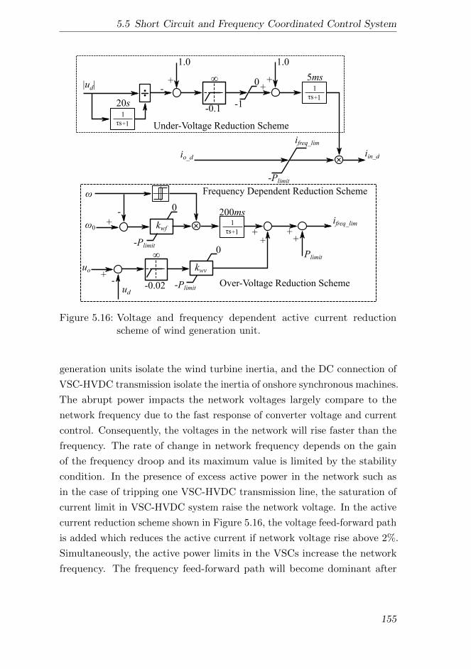
5.5 Short Circuit and Frequency Coordinated Control System

0 kwf+

-ud

ifreq_lim

+

Plimitkwv

++

+

0

0

+-

uo

-0.02

-Plimit

-Plimit

-Plimit

io_d

ifreq_lim

1

s+1

0

-1-0.1

++

+-

1.0 1.0

iin_d

|ud|

1

s+1

20s

5ms

Under-Voltage Reduction Scheme

Frequency Dependent Reduction Scheme

1

s+1

200ms

Over-Voltage Reduction Scheme

Figure 5.16: Voltage and frequency dependent active current reductionscheme of wind generation unit.

generation units isolate the wind turbine inertia, and the DC connection of

VSC-HVDC transmission isolate the inertia of onshore synchronous machines.

The abrupt power impacts the network voltages largely compare to the

network frequency due to the fast response of converter voltage and current

control. Consequently, the voltages in the network will rise faster than the

frequency. The rate of change in network frequency depends on the gain

of the frequency droop and its maximum value is limited by the stability

condition. In the presence of excess active power in the network such as

in the case of tripping one VSC-HVDC transmission line, the saturation of

current limit in VSC-HVDC system raise the network voltage. In the active

current reduction scheme shown in Figure 5.16, the voltage feed-forward path

is added which reduces the active current if network voltage rise above 2%.

Simultaneously, the active power limits in the VSCs increase the network

frequency. The frequency feed-forward path will become dominant after

155

5 Short Circuit Analysis of an Offshore AC Network

the network frequency upper limit exceeds i.e 1.004 p.u. Consequently, the

current through VSC-HVDC system comes back within its operational limits

and reinstates the reference voltage control which enforce the voltages in

the network to be within the normal operational limits. The equilibrium in

the system will be achieved at reduced wind power generation that would

be equal to the export capacity of the transmission line. However, the

steady-state network frequency will be higher than the nominal frequency.

In case of over frequency in the network, the change in network frequency

can be calculated using wind power frequency dependent reduction and the

VSC frequency droop scheme. In the offshore AC network, the sum of all

the wind turbine power is equal to the sum of the power received by the

in-service VSC-HVDC transmission systems. Thus, the condition given in

(5.11) must be satisfied.

z∑n=1

pn +

y∑m=1

pm = 0 (5.11)

Here, y is the total number of in-service VSC-HVDC system, z is the

total number of wind generation system, pn is the active power of nth wind

generation unit, and pm is the active power of mth VSC-HVDC system. The

frequency droop control equation of mth VSC-HVDC system can be defined

as (5.12) as illustrated in Figure 5.13.

ωm = ω0 − (kf m + kfs m) pm (5.12)

Note that all the impose frequencies by each VSC-HVDC system will be

equal to network frequency at steady-state, then the active power for mth

VSC-HVDC system can be defined as (5.13).

ω1 = ω2 = · · · = ωm = ω

pm =∆ω

kf m + kfs m∵ ∆ω = ω0 − ω

(5.13)

The frequency dependent wind power reduction control equation of nth

wind generation unit can be defined as (5.14).

156

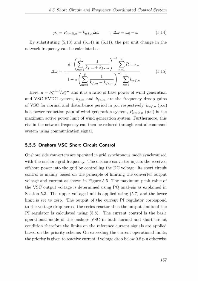
5.5 Short Circuit and Frequency Coordinated Control System

pn = Plimit n + kwf n∆ω ∵ ∆ω = ω0 − ω (5.14)

By substituting (5.13) and (5.14) in (5.11), the per unit change in the

network frequency can be calculated as

∆ω = −a ·

(y∑

m=1

1

kf m + kfs m

)−1 z∑n=1

Plimit n

1 + a

(y∑

m=1

1

kf m + kfs m

)−1 z∑n=1

kwf n

(5.15)

Here, a = Swindb /Svscb and it is a ratio of base power of wind generation

and VSC-HVDC system, kf m and kfs m are the frequency droop gains

of VSC for normal and disturbance period in p.u respectively, kwf n (p.u)

is a power reduction gain of wind generation system, Plimit n (p.u) is the

maximum active power limit of wind generation system. Furthermore, this

rise in the network frequency can then be reduced through central command

system using communication signal.

5.5.5 Onshore VSC Short Circuit Control

Onshore side converters are operated in grid synchronous mode synchronized

with the onshore grid frequency. The onshore converter injects the received

offshore power into the grid by controlling the DC voltage. Its short circuit

control is mainly based on the principle of limiting the converter output

voltage and current as shown in Figure 5.5. The maximum peak value of

the VSC output voltage is determined using PQ analysis as explained in

Section 5.3. The upper voltage limit is applied using (5.7) and the lower

limit is set to zero. The output of the current PI regulator correspond

to the voltage drop across the series reactor thus the output limits of the

PI regulator is calculated using (5.8). The current control is the basic

operational mode of the onshore VSC in both normal and short circuit

condition therefore the limits on the reference current signals are applied

based on the priority scheme. On exceeding the current operational limits,

the priority is given to reactive current if voltage drop below 0.8 p.u otherwise

157

5 Short Circuit Analysis of an Offshore AC Network

active current has priority. These current limits are applied by using (5.9)

and (5.10).

The output of the DC voltage outer controller defines the reference current

d -component and the AC voltage outer controller output defines reference

current q-component. The saturation limit values on these controllers output

are determined from Figure 5.7d. During fault, the outer control loop is

isolated due to current limits consequently converter no longer controls the

DC voltage. In this condition, the DC chopper is activated to dissipate the

excess energy in the DC link.

5.6 Simulations and Results

The methodology and control system is validated by performing nonlinear

simulation of the network shown in Figure 5.1. The network is modeled in

Simulink environment using SimPower blockset. There are five locations

within the network where faults have been applied for the analysis. First

fault is applied at the MV busbar in the wind power plant. Second fault is

applied at the HV busbar in the offshore AC network. Third fault is applied

on the interconnecting cable that connect VSC-1 and VSC-2 at the voltage

level of 150 kV. In fourth case, an open circuit fault is applied in the VSC-2.

An onshore fault has been simulated as the fifth case study. A resistive three

phase symmetrical fault of 1.0 Ω is applied for all fault analysis. In the

case studies, different aspects of VSC control for offshore and onshore short

circuit has been analyzed such as FRT capability, reduction in voltage phase

angle jump during fault, ability to operate split network after fault, and

frequency coordination scheme between VSC-HVDC transmission system

and wind generation units.

Fault at MVAC Busbar: In this case, a fault is applied at wind power plant

busbar at the voltage level of 33 kV. The fault is applied for 100 ms at 5.0 s.

The response of the VSC voltage and current is shown in Figure 5.17. It can

be observed that the voltage at the reference busbar of both VSCs drops up

to 0.4 p.u. In this condition, the VSCs are directed to inject current with

the rated peak. As the voltage drop at the reference busbar is above 0.1 p.u,

158

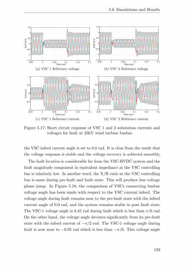
5.6 Simulations and Results

4.95 5 5.05 5.1 5.15 5.21.5

1

0.5

0

0.5

1

1.5u

3(t

) (p

.u)

Time (sec)

(a) VSC 1 Reference voltage

4.95 5 5.05 5.1 5.15 5.21.5

1

0.5

0

0.5

1

1.5

u4(t

) (p

.u)

Time (sec)

(b) VSC 2 Reference voltage

4.95 5 5.05 5.1 5.15 5.21

0.5

0

0.5

1

i 1(t

) (p

.u)

Time (sec)

(c) VSC 1 Reference current

4.95 5 5.05 5.1 5.15 5.21

0.5

0

0.5

1

i 2(t

) (p

.u)

Time (sec)

(d) VSC 2 Reference current

Figure 5.17: Short circuit response of VSC 1 and 2 substation currents andvoltages for fault at 33kV wind turbine busbar.

the VSC infeed current angle is set to 0.0 rad. It is clear from the result that

the voltage response is stable and the voltage recovery is achieved smoothly.

The fault location is considerable far from the VSC-HVDC system and the

fault magnitude component in equivalent impedance at the VSC controlling

bus is relatively low. In another word, the X/R ratio at the VSC controlling

bus is same during pre-fault and fault state. This will produce less voltage

phase jump. In Figure 5.18, the comparison of VSCs connecting busbar

voltage angle has been made with respect to the VSC current infeed. The

voltage angle during fault remains near to the pre-fault state with the infeed

current angle of 0.0 rad, and the system remains stable in post fault state.

The VSC-1 voltage angle is 0.45 rad during fault which is less than π/6 rad.

On the other hand, the voltage angle deviates significantly from its pre-fault

state with the infeed current of −π/2 rad. The VSC-1 voltage angle during

fault is now near to −0.95 rad which is less than −π/6. This voltage angle

159

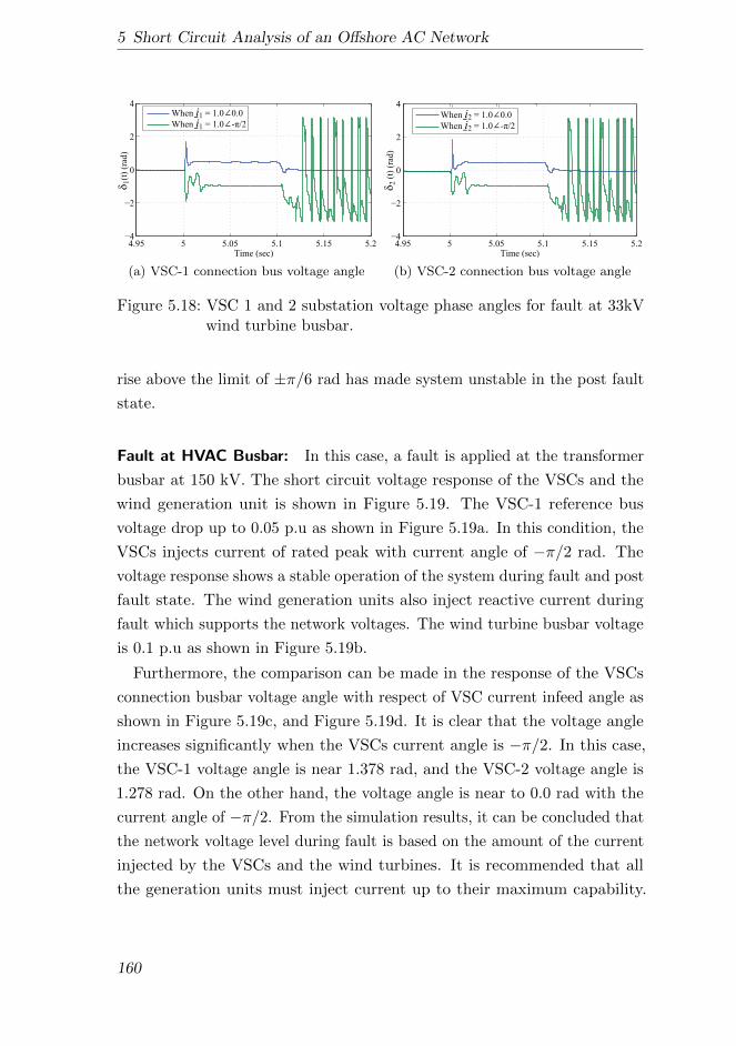
5 Short Circuit Analysis of an Offshore AC Network

4.95 5 5.05 5.1 5.15 5.24

2

0

2

4

Time (sec)

1(t

) (r

ad)

When i1 = 1.0 0.0

When i1 = 1.0 - /2

(a) VSC-1 connection bus voltage angle

4.95 5 5.05 5.1 5.15 5.24

2

0

2

4

Time (sec)

When i2 = 1.0 0.0

When i2 = 1.0 - /2

2 (

t) (

rad)

(b) VSC-2 connection bus voltage angle

Figure 5.18: VSC 1 and 2 substation voltage phase angles for fault at 33kVwind turbine busbar.

rise above the limit of ±π/6 rad has made system unstable in the post fault

state.

Fault at HVAC Busbar: In this case, a fault is applied at the transformer

busbar at 150 kV. The short circuit voltage response of the VSCs and the

wind generation unit is shown in Figure 5.19. The VSC-1 reference bus

voltage drop up to 0.05 p.u as shown in Figure 5.19a. In this condition, the

VSCs injects current of rated peak with current angle of −π/2 rad. The

voltage response shows a stable operation of the system during fault and post

fault state. The wind generation units also inject reactive current during

fault which supports the network voltages. The wind turbine busbar voltage

is 0.1 p.u as shown in Figure 5.19b.

Furthermore, the comparison can be made in the response of the VSCs

connection busbar voltage angle with respect of VSC current infeed angle as

shown in Figure 5.19c, and Figure 5.19d. It is clear that the voltage angle

increases significantly when the VSCs current angle is −π/2. In this case,

the VSC-1 voltage angle is near 1.378 rad, and the VSC-2 voltage angle is

1.278 rad. On the other hand, the voltage angle is near to 0.0 rad with the

current angle of −π/2. From the simulation results, it can be concluded that

the network voltage level during fault is based on the amount of the current

injected by the VSCs and the wind turbines. It is recommended that all

the generation units must inject current up to their maximum capability.

160

5.6 Simulations and Results

4.95 5 5.05 5.1 5.15 5.21.5

1

0.5

0

0.5

1

1.5

Time (sec)

u3 (

t) (

p.u

)

(a) VSC 1 reference bus voltage

4.95 5 5.05 5.1 5.15 5.22

1

0

1

2

Win

d T

urb

ine

Vo

ltag

e (p

.u)

Time (sec)

(b) Voltage at wind turbine busbar

4.95 5 5.05 5.1 5.15 5.24

2

0

2

4

Time (sec)

1 (

t) (

rad)

When i1 = 1.0 0.0

When i1 = 1.0 - /2

(c) VSC 1 connection bus voltage angle

4.95 5 5.05 5.1 5.15 5.24

2

0

2

4

Time (sec)

2 (t

) (r

ad)

- /2

(d) VSC 2 connection bus voltage angle

Figure 5.19: Voltage short circuit response of 150kV busbar fault.

Furthermore, the proposed short circuit scheme to mitigate the voltage phase

angle jump ensure that the phase angle remains near to its pre-fault state.

The analysis conclude that the VSC-HVDC transmission system offshore

converters current angle must be controlled according to the voltage drop in

order to ensure the network stability during fault and post fault state.

Fault at HVAC Cable: The reference frequency control of the offshore AC

network through more than one VSC-HVDC transmission systems not only

enable the trade between onshore grids but it can also operate two isolated

networks as well. To demonstrate such ability, a fault has been applied on

the cable that interconnects two VSC substations in the offshore network.

The length of the cable is 12 km. A permanent fault is applied at 5.0 s and

the AC circuit breaker at both ends of the cable is opened after 100 ms.

After fault isolation, there are two isolated networks. After isolation, wind

power plant 1 and 2 are connected with VSC-1 and the net power of these

161

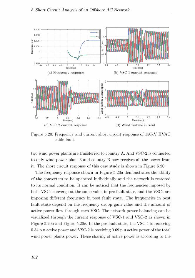
5 Short Circuit Analysis of an Offshore AC Network

4.6 4.7 4.8 4.9 5 5.1 5.2 5.3 5.40.9999

1

1

1.0001

1.0001

1.0002

1.0002

Time (sec)

Fre

quen

cy (

p.u

)1

2

(a) Frequency response

4.8 4.9 5 5.1 5.2 5.3 5.41

0.5

0

0.5

1

Time (sec)

i 1 (

t) (

p.u

)

(b) VSC 1 current response

4.8 4.9 5 5.1 5.2 5.3 5.41

0.5

0

0.5

1

Time (sec)

i 2 (

t) (

p.u

)

(c) VSC 2 current response

4.8 4.9 5 5.1 5.2 5.3 5.42

1

0

1

2

Win

d T

urb

ine

Curr

ent

(p.u

)

Time (sec)

(d) Wind turbine current

Figure 5.20: Frequency and current short circuit response of 150kV HVACcable fault.

two wind power plants are transferred to country A. And VSC-2 is connected

to only wind power plant 3 and country B now receives all the power from

it. The short circuit response of this case study is shown in Figure 5.20.

The frequency response shown in Figure 5.20a demonstrates the ability

of the converters to be operated individually and the network is restored

to its normal condition. It can be noticed that the frequencies imposed by

both VSCs converge at the same value in pre-fault state, and the VSCs are

imposing different frequency in post fault state. The frequencies in post

fault state depend on the frequency droop gain value and the amount of

active power flow through each VSC. The network power balancing can be

visualized through the current response of VSC-1 and VSC-2 as shown in

Figure 5.20b and Figure 5.20c. In the pre-fault state, the VSC-1 is receiving

0.34 p.u active power and VSC-2 is receiving 0.69 p.u active power of the total

wind power plants power. These sharing of active power is according to the

162

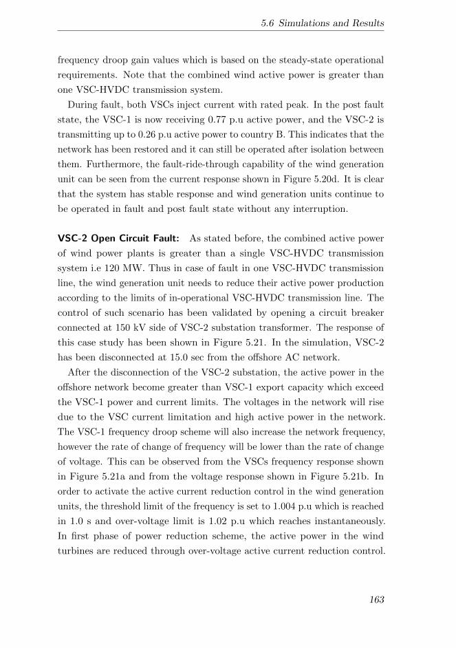
5.6 Simulations and Results

frequency droop gain values which is based on the steady-state operational

requirements. Note that the combined wind active power is greater than

one VSC-HVDC transmission system.

During fault, both VSCs inject current with rated peak. In the post fault

state, the VSC-1 is now receiving 0.77 p.u active power, and the VSC-2 is

transmitting up to 0.26 p.u active power to country B. This indicates that the

network has been restored and it can still be operated after isolation between

them. Furthermore, the fault-ride-through capability of the wind generation

unit can be seen from the current response shown in Figure 5.20d. It is clear

that the system has stable response and wind generation units continue to

be operated in fault and post fault state without any interruption.

VSC-2 Open Circuit Fault: As stated before, the combined active power

of wind power plants is greater than a single VSC-HVDC transmission

system i.e 120 MW. Thus in case of fault in one VSC-HVDC transmission

line, the wind generation unit needs to reduce their active power production

according to the limits of in-operational VSC-HVDC transmission line. The

control of such scenario has been validated by opening a circuit breaker

connected at 150 kV side of VSC-2 substation transformer. The response of

this case study has been shown in Figure 5.21. In the simulation, VSC-2

has been disconnected at 15.0 sec from the offshore AC network.

After the disconnection of the VSC-2 substation, the active power in the

offshore network become greater than VSC-1 export capacity which exceed

the VSC-1 power and current limits. The voltages in the network will rise

due to the VSC current limitation and high active power in the network.

The VSC-1 frequency droop scheme will also increase the network frequency,

however the rate of change of frequency will be lower than the rate of change

of voltage. This can be observed from the VSCs frequency response shown

in Figure 5.21a and from the voltage response shown in Figure 5.21b. In

order to activate the active current reduction control in the wind generation

units, the threshold limit of the frequency is set to 1.004 p.u which is reached

in 1.0 s and over-voltage limit is 1.02 p.u which reaches instantaneously.

In first phase of power reduction scheme, the active power in the wind

turbines are reduced through over-voltage active current reduction control.

163

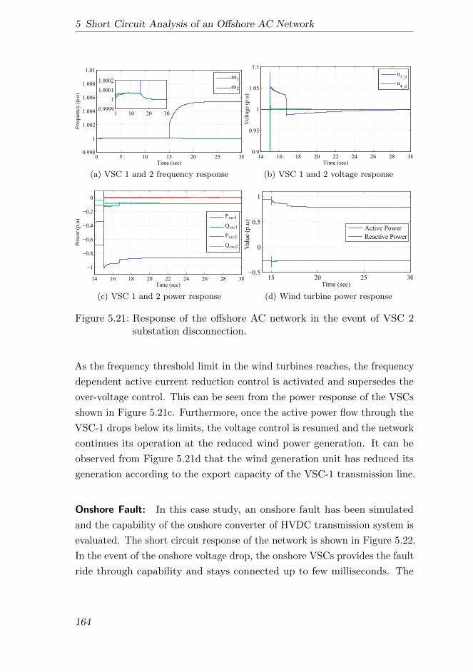
5 Short Circuit Analysis of an Offshore AC Network

0 5 10 15 20 25 300.998

1

1.002

1.004

1.006

1.008

1.01

Time (sec)

Fre

qu

ency

(p

.u)

1

2

10 20 300.9999

1

1.0001

1.0002

1

(a) VSC 1 and 2 frequency response

14 16 18 20 22 24 26 28 300.9

0.95

1

1.05

1.1

Time (sec)

Vo

ltag

e (p

.u)

u3_d

u4_d

(b) VSC 1 and 2 voltage response

14 16 18 20 22 24 26 28 30

1

0.8

0.6

0.4

0.2

0

Time (sec)

Po

wer

(p

.u)

Pvsc1

Qvsc1

Pvsc2

Qvsc2

(c) VSC 1 and 2 power response

15 20 25 300.5

0

0.5

1

Val

ue

(p.u

)

Time (sec)

Active Power

Reactive Power

(d) Wind turbine power response

Figure 5.21: Response of the offshore AC network in the event of VSC 2substation disconnection.

As the frequency threshold limit in the wind turbines reaches, the frequency

dependent active current reduction control is activated and supersedes the

over-voltage control. This can be seen from the power response of the VSCs

shown in Figure 5.21c. Furthermore, once the active power flow through the

VSC-1 drops below its limits, the voltage control is resumed and the network

continues its operation at the reduced wind power generation. It can be

observed from Figure 5.21d that the wind generation unit has reduced its

generation according to the export capacity of the VSC-1 transmission line.

Onshore Fault: In this case study, an onshore fault has been simulated

and the capability of the onshore converter of HVDC transmission system is

evaluated. The short circuit response of the network is shown in Figure 5.22.

In the event of the onshore voltage drop, the onshore VSCs provides the fault

ride through capability and stays connected up to few milliseconds. The

164

5.6 Simulations and Results

4.8 5.0 5.2 5.4 5.6 5.8

0.0

0.5

1.0

Time (sec)

Vo

ltag

e (p

.u) ud

uq

-0.4

1.4

(a) Onshore VSC filter bus voltages

4.8 5.0 5.2 5.4 5.6 5.8-1.0

-0.5

0.0

0.5

1.0

Time (sec)

Cu

rren

t (p

.u)

id

iq

(b) Current injected by onshore VSC

4.8 5 5.2 5.4 5.6 5.80.98

0.99

1.00

1.01

1.02

Time (sec)

Volt

age

(p.u

)

Udc_offshore

Udc_onshore

(c) DC voltage at onshore and offshore DCbubar

4.8 5 5.2 5.4 5.6 5.81

0.5

0

0.5

1

Time (sec)

Val

ue

(p.u

)

pvsc1

qvsc1

(d) Active and reactive power response ofVSC-1 (offshore)

Figure 5.22: The network short circuit voltage and current response of thefault applied at country A onshore grid.

DC voltage of the HVDC transmission system is then controlled through a

chopper that dissipate energy through the DC resistor.

To evaluate the onshore converter short circuit control system, the country-

A onshore grid voltage is dropped to 0.1 p.u at 5.0 s for 100 ms. The response

of the onshore VSC voltage in dq0 frame is shown in Figure 5.22a. Typically,

it is defined in the transmission system grid code that the generation units

must inject reactive current during fault to support the grid voltage. In this

regard, the onshore VSC injects the reactive current which can be observed

from Figure 5.22b. It can be seen that the current d -component reduces

to zero and the q-component is increased for maximum reactive current

injection. In the post fault state, both current components are restored as

fast as possible in order to maintain the network stability. The DC voltage

response at both ends of the DC cable is shown in Figure 5.22c. Since the PI

165

5 Short Circuit Analysis of an Offshore AC Network

control of the onshore VSC DC voltage control is isolated during fault, the

DC voltage is no longer controlled to 1.0 p.u. Instead the chopper control,

which is like a proportional controller, maintain the DC voltage. It can be

seen from the DC voltage response that the voltages remain with in the

limit at both ends. Although, the offshore VSC has DC voltage independent

control scheme but the ability of a converter to generate AC output voltage

depends on the DC voltage. The variation in the DC voltage may appear

on the AC output voltage consequently effect the power flow through the

VSC. This can be observed through the power response of VSC-1 shown in

Figure 5.22d. These variations can be minimized by increasing the stiffness

of the offshore VSC voltage control.

5.7 Summary

This chapter presents the control system of the VSC-HVDC system for an

offshore AC network for normal and short circuit operation. The offshore AC

network is created by two VSCs using frequency and voltage droop control

schemes. During short circuit, both VSCs inject current up to their maximum

capability. It has been concluded that the VSCs must inject active current to

ensure the system stability for the fault voltage above 0.1 p.u. Furthermore,

the reactive current injection by the VSCs improves the network voltages

for low voltage fault and keeps the network bus voltage angle near to pre-

fault state. Through simulation, it has been proven that the control of the

offshore AC network reference voltage and frequency via more than one VSC-

HVDC system provides operational redundancy and the network can still

be operated if isolation occurs between VSC-HVDC systems. Furthermore,

the proposed coordinated control ensure the continuous operation of the

network at reduced export capacity. The presented study and proposed

control system can be a useful tool for establishing offshore grid codes.

166

6 Analysis of Hybrid AC/DC

Offshore Grid

The focus of this chapter is on the application of integrating an offshore

AC grid with an offshore DC grid. The future ‘SuperGrid’ may require

the benefit of both offshore AC network and MTDC grid. To analyze the

integrated AC and DC network, first the basic principle of the MTDC

network control is discussed. Later, the aspects of the MTDC operation

are addressed with respect to the VSCs ability to control the wind power

distribution. The DC voltage droop control is applied for the distributed

control of the MTDC network. The active power infeed into onshore grids

has fluctuation according to the wind variation. In order to flow the constant

power between onshore grids via offshore MTDC network, the dead-band

droop control scheme is implemented in the onshore VSCs control system.

The network operational principle has been demonstrated using nonlinear

simulation. In the end, the operation of the combined offshore AC network

and MTDC network is demonstrated.

6.1 Introduction

An efficient, economical, and reliable offshore wind power plant transmission

system has utmost importance for the development of the future ‘SuperGrid’

[118]. The selection between the HVAC or HVDC transmission for the

offshore wind power plant connection mainly depends on its distance from

the shore and the installed capacity [119]. For the long distances, HVDC

transmission system has preference over HVAC cables since the latter has

higher losses and requires additional reactive power compensation. The

offshore wind power plants located within the distance of 60 km from

167

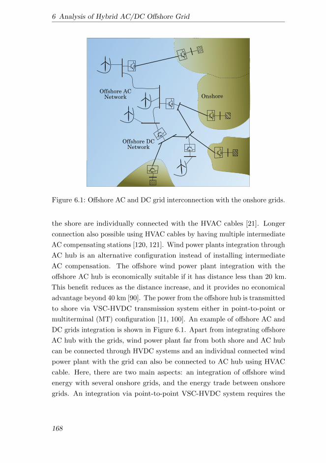
6 Analysis of Hybrid AC/DC Offshore Grid

Offshore DC

Network

Offshore AC

Network Onshore

Figure 6.1: Offshore AC and DC grid interconnection with the onshore grids.

the shore are individually connected with the HVAC cables [21]. Longer

connection also possible using HVAC cables by having multiple intermediate

AC compensating stations [120, 121]. Wind power plants integration through

AC hub is an alternative configuration instead of installing intermediate

AC compensation. The offshore wind power plant integration with the

offshore AC hub is economically suitable if it has distance less than 20 km.

This benefit reduces as the distance increase, and it provides no economical

advantage beyond 40 km [90]. The power from the offshore hub is transmitted

to shore via VSC-HVDC transmission system either in point-to-point or

multiterminal (MT) configuration [11, 100]. An example of offshore AC and

DC grids integration is shown in Figure 6.1. Apart from integrating offshore

AC hub with the grids, wind power plant far from both shore and AC hub

can be connected through HVDC systems and an individual connected wind

power plant with the grid can also be connected to AC hub using HVAC

cable. Here, there are two main aspects: an integration of offshore wind

energy with several onshore grids, and the energy trade between onshore

grids. An integration via point-to-point VSC-HVDC system requires the

168

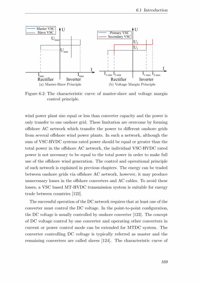
6.1 Introduction

I

U

Imax

Imin

Umax

Umin

InverterRectifier

Master VSC

Slave VSC

(a) Master-Slave Principle

I

U

I2-maxI2-min

InverterRectifier

Primary VSCSecondary VSC

U2

U1

I1-maxI1-min

(b) Voltage Margin Principle

Figure 6.2: The characteristic curve of master-slave and voltage margincontrol principle.

wind power plant size equal or less than converter capacity and the power is

only transfer to one onshore grid. These limitation are overcome by forming

offshore AC network which transfer the power to different onshore grids

from several offshore wind power plants. In such a network, although the

sum of VSC-HVDC systems rated power should be equal or greater than the

total power in the offshore AC network, the individual VSC-HVDC rated

power is not necessary to be equal to the total power in order to make full

use of the offshore wind generation. The control and operational principle

of such network is explained in previous chapters. The energy can be traded

between onshore grids via offshore AC network, however, it may produce

unnecessary losses in the offshore converters and AC cables. To avoid these

losses, a VSC based MT-HVDC transmission system is suitable for energy

trade between countries [122].

The successful operation of the DC network requires that at least one of the

converter must control the DC voltage. In the point-to-point configuration,

the DC voltage is usually controlled by onshore converter [123]. The concept

of DC voltage control by one converter and operating other converters in

current or power control mode can be extended for MTDC system. The

converter controlling DC voltage is typically referred as master and the

remaining converters are called slaves [124]. The characteristic curve of

169

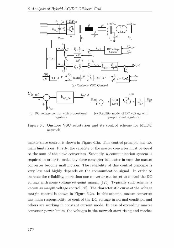
6 Analysis of Hybrid AC/DC Offshore Grid

i

Udc

lg rg

Cdc

Il Idc

uv u un

kp+kis

kp+kis

+

-+

+-

+

-

++

+

T-1( (t))

id

iq

ud

uq

l

l

iref_d

iref_q

uv_d

uv_q

uv_abc

T( (t))T( (t))u i

(t) uduq

idiq

110kVLL 220kVLL

112MVA

g

Udc_ref

Udc

PLLu

+

p

q

idq

udqp

q udq idq=s

gg

gg

g

g

cg

ud

uac_ref koi_ac

skop_ac +g

g

-

DC VoltageControl

(a) Onshore VSC Control

kop_dc

Udc_ref

Udc

iref_d

(b) DC voltage control with proportionalregulator

is+1

G(s)Ur (s) 1Cdcs

U(s)

Il (s)

(c) Stability model of DC voltage withproportional regulator

Figure 6.3: Onshore VSC substation and its control scheme for MTDCnetwork.

master-slave control is shown in Figure 6.2a. This control principle has two

main limitations. Firstly, the capacity of the master converter must be equal

to the sum of the slave converters. Secondly, a communication system is

required in order to make any slave converter to master in case the master

converter become malfunction. The reliability of this control principle is

very low and highly depends on the communication signal. In order to

increase the reliability, more than one converter can be set to control the DC

voltage with some voltage set-point margin [125]. Typically such scheme is

known as margin voltage control [56]. The characteristic curve of the voltage

margin control is shown in Figure 6.2b. In this scheme, master converter

has main responsibility to control the DC voltage in normal condition and

others are working in constant current mode. In case of exceeding master

converter power limits, the voltages in the network start rising and reaches

170

6.2 Multiterminal VSC-HVDC System

voltage threshold limits at the slave converter busbar, hereby enforcing slave

converter to regulate DC voltage instead of current [126]. In this control

scheme, it is important that the master converter voltage set-point must be

less than the slave converter threshold limit. As a disadvantage, the voltage

margin control only allow fixed power sharing and it needs several control

loops which make the voltage regulation slower [57].

Usually, any DC voltage regulation that requires communication at some

extent are considered as centralized control system. A decentralized control

system such as droop control increases the controllability and reliability in

the system. The principle of the droop control is similar to the frequency

regulation in the AC system. In this control scheme, all or selected onshore

converters in the MTDC offshore network can have the droop control in

order to control the DC voltages. In the droop control, the change in DC

power received by the converter proportionally changes the DC voltage. For

a stiff voltage control, the net power in the offshore DC grid can then be

shared among onshore converters by adjusting the slope of the droop values.

Furthermore, the network can be operated even if one or more onshore

converters malfunction [127].

6.2 Multiterminal VSC-HVDC System

In the MTDC system for the offshore wind integration, all the onshore side

VSCs can be set to control the DC voltage. A concept of the DC voltage

control of VSC in point-to-point configuration is explained in Section 2.3.

Usually, the DC resistance in the network is relatively small even for long

cables (e.g 0.019 Ω/km). The DC voltage control using proportional-plus

integral (PI) regulator in the MTDC system makes VSCs to react as voltage

sources connecting in parallel at the common bus with very low equivalent

resistance. This could cause large active power flow among them and lead

system into instability. Thus, a proportional (P) control can be applied

instead of PI regulator for DC voltage control. A proportional controller

does not enforce the bus voltage at the given set-point rather the error in

the voltage from the set-point enable the balancing of the network through

multiple VSCs. The modified onshore substation and its control system is

171

6 Analysis of Hybrid AC/DC Offshore Grid

I

U

I3

Inverter Rectifier

Ur

I1

I2

VSC-1

VSC-2

VSC-3

Figure 6.4: U-I characteristic of onshore VSCs DC voltage control to operateMTDC network.

shown in Figure 6.3 for MTDC network.

The feed-forward network current input (Il) is removed to control with

only voltage feedback signal to avoid conflict between VSCs in MTDC

configuration. Note that the summation sign shown in Figure 6.3b are

reversed to adjust the sign convention between DC and AC network. The

closed loop transfer function can be derived from the stability model of the

DC voltage control of a VSC given in Figure 6.3c.

U(s) =G(s)Ur(s) + (τis+ 1)Il(s)

Cdcτis2 + Cdcs+G(s)(6.1)

Here, τi is the time constant of the current closed loop, Cdc is the DC

capacitance, G(s) is the DC voltage controller, Ur(s) is the voltage set-point,

Il(s) is the network current, and U(s) is the output voltage. Note that

the closed loop transfer function given in (6.1) represents a single VSC

DC voltage control dynamics. The stability conditions of only one VSC

controlling DC voltage in the DC network are: τi > 0 and kop dc > 0. Using

(6.1), the steady-state DC voltage equation of a VSC can be determined by

setting all the derivatives to zero i.e s→ 0.

U(s) = Ur(s) +1

kop dcIl(s) ∵ G(s) = kop dc

U(s) = Ur(s)−1

kop dcIdc(s) ∵ Il(s) + Idc(s) = 0

(6.2)

172

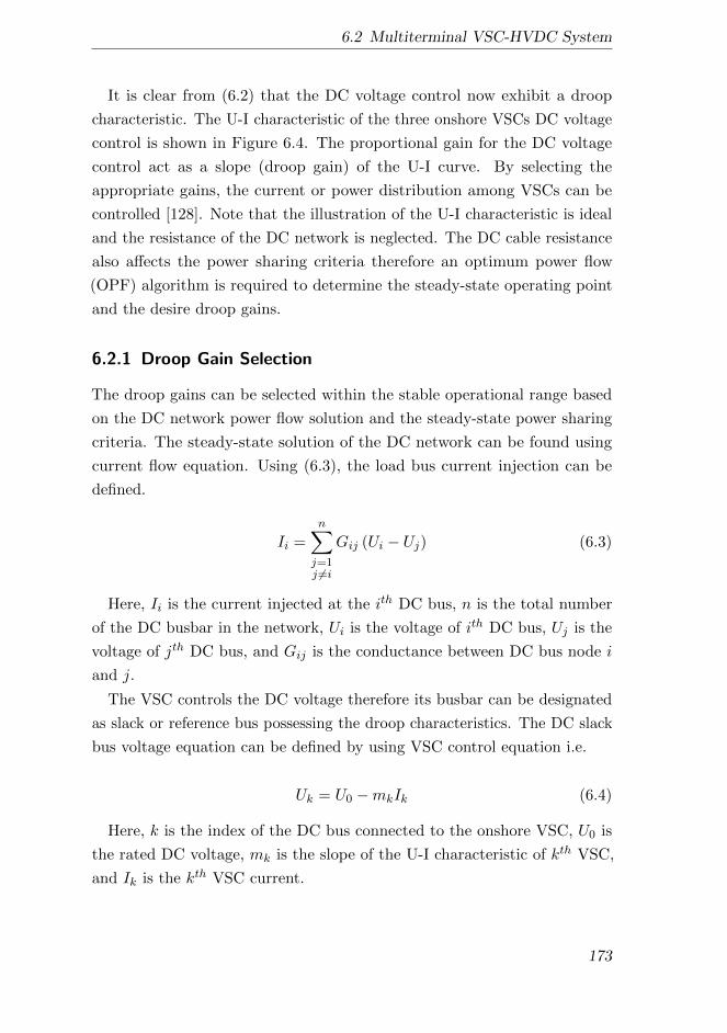
6.2 Multiterminal VSC-HVDC System

It is clear from (6.2) that the DC voltage control now exhibit a droop

characteristic. The U-I characteristic of the three onshore VSCs DC voltage

control is shown in Figure 6.4. The proportional gain for the DC voltage

control act as a slope (droop gain) of the U-I curve. By selecting the

appropriate gains, the current or power distribution among VSCs can be

controlled [128]. Note that the illustration of the U-I characteristic is ideal

and the resistance of the DC network is neglected. The DC cable resistance

also affects the power sharing criteria therefore an optimum power flow

(OPF) algorithm is required to determine the steady-state operating point

and the desire droop gains.

6.2.1 Droop Gain Selection

The droop gains can be selected within the stable operational range based

on the DC network power flow solution and the steady-state power sharing

criteria. The steady-state solution of the DC network can be found using

current flow equation. Using (6.3), the load bus current injection can be

defined.

Ii =n∑j=1j 6=i

Gij (Ui − Uj) (6.3)

Here, Ii is the current injected at the ith DC bus, n is the total number

of the DC busbar in the network, Ui is the voltage of ith DC bus, Uj is the

voltage of jth DC bus, and Gij is the conductance between DC bus node i

and j.

The VSC controls the DC voltage therefore its busbar can be designated

as slack or reference bus possessing the droop characteristics. The DC slack

bus voltage equation can be defined by using VSC control equation i.e.

Uk = U0 −mkIk (6.4)

Here, k is the index of the DC bus connected to the onshore VSC, U0 is

the rated DC voltage, mk is the slope of the U-I characteristic of kth VSC,

and Ik is the kth VSC current.

173

6 Analysis of Hybrid AC/DC Offshore Grid

The OPF algorithm can be implemented using MATLAB function ‘fmincon’

using interior-point method to solve the network equations. The network

equations are applied as equality constraints. Further, the OPF algorithm

provides the network voltages and currents as the results. The slope of the

droop (mk) can also be determined based on the current sharing criteria

among onshore VSCs. The current of the kth VSC can be written as the

sharing factor of the total current received by all the DC voltage control

VSCs.

Ik = αkItot (6.5)

Here, αk is the current sharing factor of kth VSC, and Itot is the sum

of all the VSC current that has droop characteristic. For any z converters

controlling DC voltage, Itot can be calculated as

Itot =

z∑j=1

Ij (6.6)

By substituting (6.6) in (6.5), the current sharing equation can be defined

for any kth DC voltage controlling VSC as given in (6.7). Furthermore, the

sharing factor must satisfy the condition given in (6.8).

(1− αk) Ik − αkz∑j=1j 6=k

Ij = 0 (6.7)

z∑j=1

αj = 1 (6.8)

The state variables of the OPF algorithm can be defined as

x =[U1 · · ·Un, I1 · · · Iz,m1 · · ·mz

]∴ kop dc z =

1

mz(6.9)

Note that the VSC voltage controller proportional gain is the reciprocal

of the droop gain, and the OPF algorithm only provides the solution based

on the steady-state requirements. Therefore, the upper and lower boundary

of the state variables must be defined by considering their stable operational

174

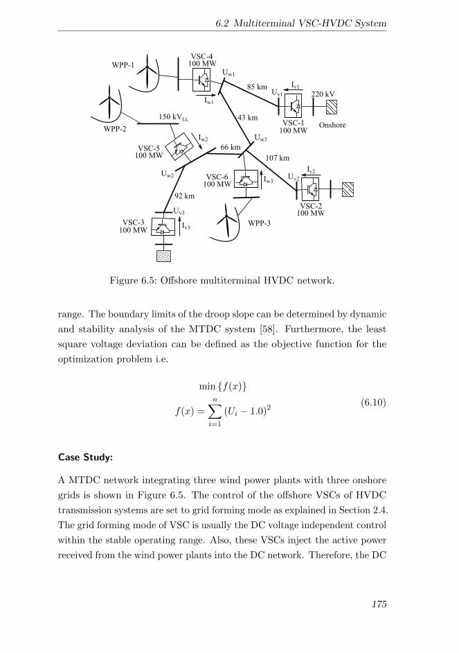
6.2 Multiterminal VSC-HVDC System

Onshore

150 kVLL

220 kV

85 km

43 km

107 km

66 km

92 km

100 MW

100 MW

100 MW

100 MW

100 MW

100 MWWPP-1

WPP-2

WPP-3

VSC-4

VSC-5

VSC-6

VSC-1

VSC-2

VSC-3

Iw3

Iw1

Iw2

Iv1

Iv2

Iv3

Uw1

Uw3

Uw2

Uv1

Uv2

Uv3

Figure 6.5: Offshore multiterminal HVDC network.

range. The boundary limits of the droop slope can be determined by dynamic

and stability analysis of the MTDC system [58]. Furthermore, the least

square voltage deviation can be defined as the objective function for the

optimization problem i.e.

min f(x)

f(x) =

n∑i=1

(Ui − 1.0)2(6.10)

Case Study:

A MTDC network integrating three wind power plants with three onshore

grids is shown in Figure 6.5. The control of the offshore VSCs of HVDC

transmission systems are set to grid forming mode as explained in Section 2.4.

The grid forming mode of VSC is usually the DC voltage independent control

within the stable operating range. Also, these VSCs inject the active power

received from the wind power plants into the DC network. Therefore, the DC

175

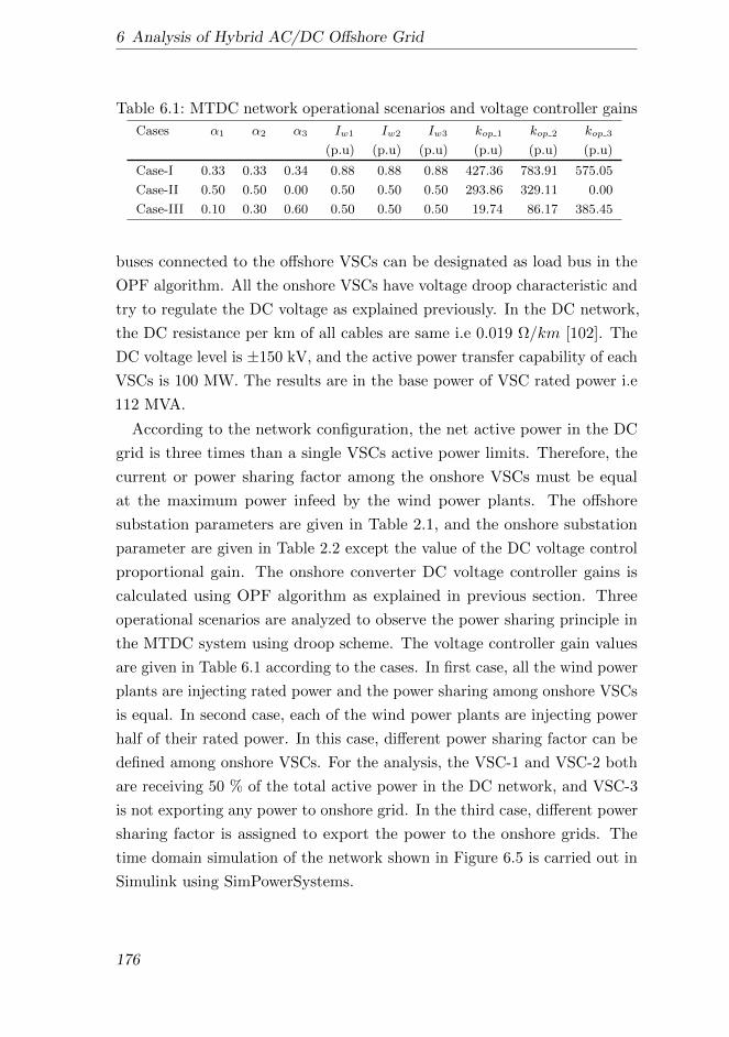
6 Analysis of Hybrid AC/DC Offshore Grid

Table 6.1: MTDC network operational scenarios and voltage controller gains

Cases α1 α2 α3 Iw1 Iw2 Iw3 kop 1 kop 2 kop 3

(p.u) (p.u) (p.u) (p.u) (p.u) (p.u)

Case-I 0.33 0.33 0.34 0.88 0.88 0.88 427.36 783.91 575.05

Case-II 0.50 0.50 0.00 0.50 0.50 0.50 293.86 329.11 0.00

Case-III 0.10 0.30 0.60 0.50 0.50 0.50 19.74 86.17 385.45

buses connected to the offshore VSCs can be designated as load bus in the

OPF algorithm. All the onshore VSCs have voltage droop characteristic and

try to regulate the DC voltage as explained previously. In the DC network,

the DC resistance per km of all cables are same i.e 0.019 Ω/km [102]. The

DC voltage level is ±150 kV, and the active power transfer capability of each

VSCs is 100 MW. The results are in the base power of VSC rated power i.e

112 MVA.

According to the network configuration, the net active power in the DC

grid is three times than a single VSCs active power limits. Therefore, the

current or power sharing factor among the onshore VSCs must be equal

at the maximum power infeed by the wind power plants. The offshore

substation parameters are given in Table 2.1, and the onshore substation

parameter are given in Table 2.2 except the value of the DC voltage control

proportional gain. The onshore converter DC voltage controller gains is

calculated using OPF algorithm as explained in previous section. Three

operational scenarios are analyzed to observe the power sharing principle in

the MTDC system using droop scheme. The voltage controller gain values

are given in Table 6.1 according to the cases. In first case, all the wind power

plants are injecting rated power and the power sharing among onshore VSCs

is equal. In second case, each of the wind power plants are injecting power

half of their rated power. In this case, different power sharing factor can be

defined among onshore VSCs. For the analysis, the VSC-1 and VSC-2 both

are receiving 50 % of the total active power in the DC network, and VSC-3

is not exporting any power to onshore grid. In the third case, different power

sharing factor is assigned to export the power to the onshore grids. The

time domain simulation of the network shown in Figure 6.5 is carried out in

Simulink using SimPowerSystems.

176

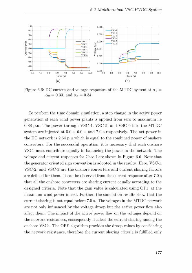
6.2 Multiterminal VSC-HVDC System

3.0 4.0 5.0 6.0 7.0 8.0 9.0 10.0

Time (s)

-1.0

-0.8

-0.6

-0.4

-0.2

0.0

0.2

0.4

0.6

0.8

1.0C

urr

ent

(p.u

) VSC-1

VSC-2

VSC-3

VSC-4

VSC-5

VSC-6

(a)

3.0 4.0 5.0 6.0 7.0 8.0 9.0 10.0

Time (s)

0.998

1.000

1.002

1.004

1.006

1.008

1.010

Vo

ltag

e (p

.u)

VSC-1

VSC-2

VSC-3

VSC-4

VSC-5

VSC-6

(b)

Figure 6.6: DC current and voltage responses of the MTDC system at α1 =α2 = 0.33, and α3 = 0.34.

To perform the time domain simulation, a step change in the active power

generation of each wind power plants is applied from zero to maximum i.e

0.88 p.u. The power through VSC-4, VSC-5, and VSC-6 into the MTDC

system are injected at 5.0 s, 6.0 s, and 7.0 s respectively. The net power in

the DC network is 2.64 p.u which is equal to the combined power of onshore

converters. For the successful operation, it is necessary that each onshore

VSCs must contribute equally in balancing the power in the network. The

voltage and current responses for Case-I are shown in Figure 6.6. Note that

the generator oriented sign convention is adopted in the results. Here, VSC-1,

VSC-2, and VSC-3 are the onshore converters and current sharing factors

are defined for them. It can be observed from the current response after 7.0 s

that all the onshore converters are sharing current equally according to the

designed criteria. Note that the gain value is calculated using OPF at the

maximum wind power infeed. Further, the simulation results show that the

current sharing is not equal before 7.0 s. The voltages in the MTDC network

are not only influenced by the voltage droop but the active power flow also

affect them. The impact of the active power flow on the voltages depend on

the network resistances, consequently it affect the current sharing among the

onshore VSCs. The OPF algorithm provides the droop values by considering

the network resistance, therefore the current sharing criteria is fulfilled only

177

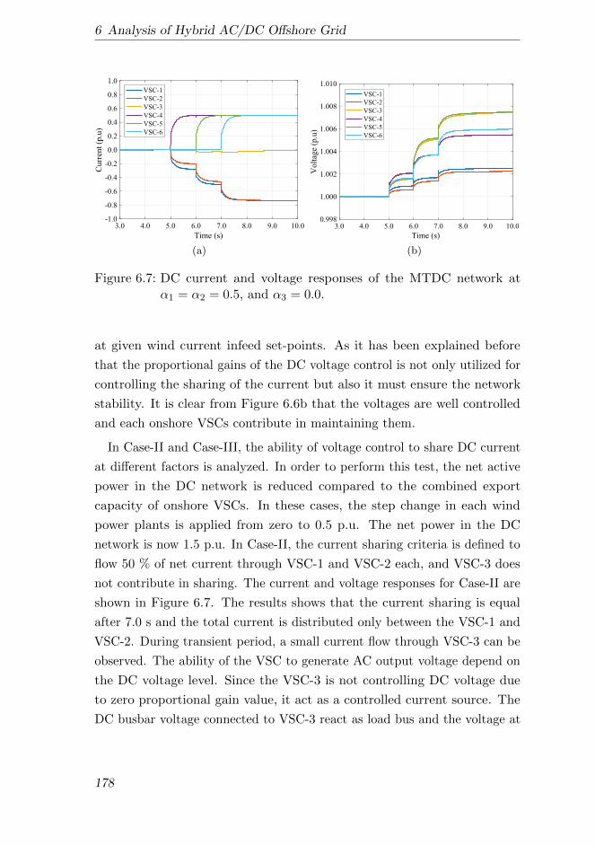
6 Analysis of Hybrid AC/DC Offshore Grid

3.0 4.0 5.0 6.0 7.0 8.0 9.0 10.0

Time (s)

-1.0

-0.8

-0.6

-0.4

-0.2

0.0

0.2

0.4

0.6

0.8

1.0

Curr

ent

(p.u

)VSC-1

VSC-2

VSC-3

VSC-4

VSC-5

VSC-6

(a)

3.0 4.0 5.0 6.0 7.0 8.0 9.0 10.0

Time (s)

0.998

1.000

1.002

1.004

1.006

1.008

1.010

Vo

ltag

e (p

.u)

VSC-1

VSC-2

VSC-3

VSC-4

VSC-5

VSC-6

(b)

Figure 6.7: DC current and voltage responses of the MTDC network atα1 = α2 = 0.5, and α3 = 0.0.

at given wind current infeed set-points. As it has been explained before

that the proportional gains of the DC voltage control is not only utilized for

controlling the sharing of the current but also it must ensure the network

stability. It is clear from Figure 6.6b that the voltages are well controlled

and each onshore VSCs contribute in maintaining them.

In Case-II and Case-III, the ability of voltage control to share DC current

at different factors is analyzed. In order to perform this test, the net active

power in the DC network is reduced compared to the combined export

capacity of onshore VSCs. In these cases, the step change in each wind

power plants is applied from zero to 0.5 p.u. The net power in the DC

network is now 1.5 p.u. In Case-II, the current sharing criteria is defined to

flow 50 % of net current through VSC-1 and VSC-2 each, and VSC-3 does

not contribute in sharing. The current and voltage responses for Case-II are

shown in Figure 6.7. The results shows that the current sharing is equal

after 7.0 s and the total current is distributed only between the VSC-1 and

VSC-2. During transient period, a small current flow through VSC-3 can be

observed. The ability of the VSC to generate AC output voltage depend on

the DC voltage level. Since the VSC-3 is not controlling DC voltage due

to zero proportional gain value, it act as a controlled current source. The

DC busbar voltage connected to VSC-3 react as load bus and the voltage at

178

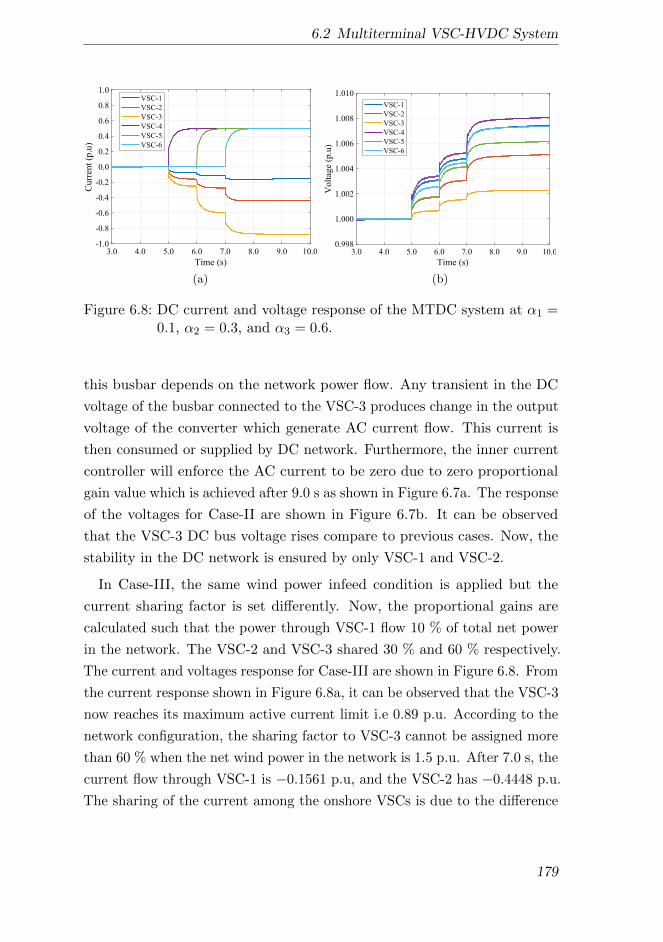
6.2 Multiterminal VSC-HVDC System

3.0 4.0 5.0 6.0 7.0 8.0 9.0 10.0

Time (s)

-1.0

-0.8

-0.6

-0.4

-0.2

0.0

0.2

0.4

0.6

0.8

1.0C

urr

ent

(p.u

)

VSC-1

VSC-2

VSC-3

VSC-4

VSC-5

VSC-6

(a)

3.0 4.0 5.0 6.0 7.0 8.0 9.0 10.0

Time (s)

0.998

1.000

1.002

1.004

1.006

1.008

1.010

Vo

ltag

e (p

.u)

VSC-1

VSC-2

VSC-3

VSC-4

VSC-5

VSC-6

(b)

Figure 6.8: DC current and voltage response of the MTDC system at α1 =0.1, α2 = 0.3, and α3 = 0.6.

this busbar depends on the network power flow. Any transient in the DC

voltage of the busbar connected to the VSC-3 produces change in the output

voltage of the converter which generate AC current flow. This current is

then consumed or supplied by DC network. Furthermore, the inner current

controller will enforce the AC current to be zero due to zero proportional

gain value which is achieved after 9.0 s as shown in Figure 6.7a. The response

of the voltages for Case-II are shown in Figure 6.7b. It can be observed

that the VSC-3 DC bus voltage rises compare to previous cases. Now, the

stability in the DC network is ensured by only VSC-1 and VSC-2.

In Case-III, the same wind power infeed condition is applied but the

current sharing factor is set differently. Now, the proportional gains are

calculated such that the power through VSC-1 flow 10 % of total net power

in the network. The VSC-2 and VSC-3 shared 30 % and 60 % respectively.

The current and voltages response for Case-III are shown in Figure 6.8. From

the current response shown in Figure 6.8a, it can be observed that the VSC-3

now reaches its maximum active current limit i.e 0.89 p.u. According to the

network configuration, the sharing factor to VSC-3 cannot be assigned more

than 60 % when the net wind power in the network is 1.5 p.u. After 7.0 s, the

current flow through VSC-1 is −0.1561 p.u, and the VSC-2 has −0.4448 p.u.

The sharing of the current among the onshore VSCs is due to the difference

179

6 Analysis of Hybrid AC/DC Offshore Grid

I

U

Inverter Rectifier

Ur

VSC-1

VSC-2

VSC-3

U

Umax

Umin

(a) Droop principle with dead-bandcharacteristics

kop_dcUmax

Udciref_d

kop_dcUmin

Iset

2.0

0.0

0.0

-2.0

(b) DC voltage control with dead-bandcharacteristic

Figure 6.9: The dead-band droop characteristic and its control system.

in the busbar voltages of the VSCs. The change in the network voltages are

mainly caused by droop characteristics of voltage controller. While selecting

the proportional gain with respect of sharing criteria, it is also important

to keep the network voltage within the operational limits. The voltages

response shown in Figure 6.8b indicate that the change in network voltages

are less than 1.0 %. The results show that the power or current distribution

can be achieved through DC voltage controller while maintaining the DC

network stability. Also, all the onshore VSCs are controlling DC voltage

which provides the redundancy in the MTDC network.

6.2.2 Dead-Band Droop Control

The flow of DC current in the MTDC network can be controlled by adjusting

the proportional gain of the DC voltage control as demonstrated in the

previous section. Although, the distribution of the wind power infeed among

onshore VSCs into the MTDC network is relatively easy but a constant

power export is difficult between two onshore grids. A droop principle can be

combined with constant current scheme in order to achieve export between

onshore grids. This scheme is commonly known as dead-band droop control.

The dead-band droop characteristic curve is illustrated in Figure 6.9a. In

the MTDC network control principle, at least one of the VSC must have the

180

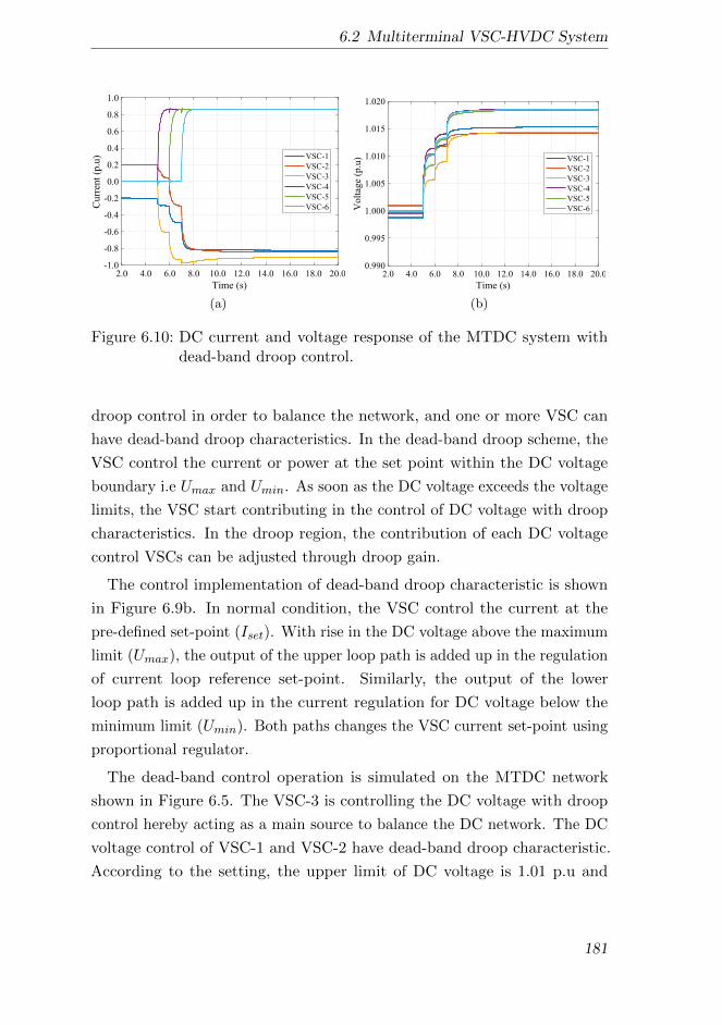
6.2 Multiterminal VSC-HVDC System

2.0 4.0 6.0 8.0 10.0 12.0 14.0 16.0 18.0 20.0

Time (s)

-1.0

-0.8

-0.6

-0.4

-0.2

0.0

0.2

0.4

0.6

0.8

1.0C

urr

ent

(p.u

) VSC-1

VSC-2

VSC-3

VSC-4

VSC-5

VSC-6

(a)

2.0 4.0 6.0 8.0 10.0 12.0 14.0 16.0 18.0 20.0

Time (s)

0.990

0.995

1.000

1.005

1.010

1.015

1.020

Vo

ltag

e (p

.u) VSC-1

VSC-2

VSC-3

VSC-4

VSC-5

VSC-6

(b)

Figure 6.10: DC current and voltage response of the MTDC system withdead-band droop control.

droop control in order to balance the network, and one or more VSC can

have dead-band droop characteristics. In the dead-band droop scheme, the

VSC control the current or power at the set point within the DC voltage

boundary i.e Umax and Umin. As soon as the DC voltage exceeds the voltage

limits, the VSC start contributing in the control of DC voltage with droop

characteristics. In the droop region, the contribution of each DC voltage

control VSCs can be adjusted through droop gain.

The control implementation of dead-band droop characteristic is shown

in Figure 6.9b. In normal condition, the VSC control the current at the

pre-defined set-point (Iset). With rise in the DC voltage above the maximum

limit (Umax), the output of the upper loop path is added up in the regulation

of current loop reference set-point. Similarly, the output of the lower

loop path is added up in the current regulation for DC voltage below the

minimum limit (Umin). Both paths changes the VSC current set-point using

proportional regulator.

The dead-band control operation is simulated on the MTDC network

shown in Figure 6.5. The VSC-3 is controlling the DC voltage with droop

control hereby acting as a main source to balance the DC network. The DC

voltage control of VSC-1 and VSC-2 have dead-band droop characteristic.

According to the setting, the upper limit of DC voltage is 1.01 p.u and

181

6 Analysis of Hybrid AC/DC Offshore Grid

the lower limit is 0.99 p.u. The gain values of the DC voltage proportional

control of VSC-1, VSC-2, and VSC-3 are 120 p.u, 250 p.u, and 100 p.u.

The current and voltage responses of the system are shown in Figure 6.10.

Initially, VSC-2 is set to export 0.2 p.u energy and VSC-1 is set to import

0.2 p.u. In the absence of wind power in the DC network, VSC-3 does not

import or export power since the net power is balanced between VSC-1 and

VSC-2. With the injection of the wind power, the VSC-3 start receiving

this power to balance the network until the DC voltages at the VSC-1 and

VSC-2 busbar reach the upper limit. Once the busbars voltage exceed the

limits, all the onshore VSCs then import the wind power. The contribution

of each VSCs in balancing the power in the DC network can be adjusted by

the voltage limits and proportional gains.

6.3 Integration of Offshore AC and DC Grids

The realization of a ‘SuperGrid’ at the North and Baltic Sea may require

the benefits of both offshore AC collector system and MTDC networks. An

offshore AC network allows the centralized collection of offshore energies

located at long distances, and the MTDC network can provide the mean

of transferring this collected energy at different onshore grids and enable

the trade between them. An example of an offshore grid formed by the

combination of offshore AC network and MTDC network is shown in Fi-

gure 6.11. In the network, three wind power plants are connected together

with HVAC cables to form offshore AC collector system. The fourth wind

power plant is located far from both onshore grids and the collector system

therefore it is interlinked with the HVDC system. Three onshore grids

are connected with the offshore AC collector system via MT-VSC HVDC

transmission system, and an onshore grid is interconnected with the AC

collector system via VSC-HVDC system in the point-to-point configuration.

All the VSCs have the same rated active power i.e 100 MW, and the rated

apparent power is 112 MVA. The network voltages and cables parameters

are given in Table 6.2.

The offshore VSCs ‘Off-VSC-1’, ‘Off-VSC-2’, and ‘Off-VSC-3’ are opera-

ting in the grid forming mode with frequency and voltage droop schemes

182

6.3 Integration of Offshore AC and DC Grids

Off-VSC-1

Off-VSC-2

Off-VSC-3

OnshoreOffshore

7 km

18 km

4 km

15 km

6 km

1 km

100 km

85 km

43 km

107 km66 km

92 km

110 MW

90 MW

40 MW

100 MW

WPP-1

WPP-2

WPP-3

WPP-4

Grid-1

Grid-2

Grid-3

Grid-4

100 MW

100 MW

100 MW

100 MW

100 MW

100 MW

100 MW

100 MW

Off-VSC-4

On-VSC-1

On-VSC-2

On-VSC-3

On-VSC-4

AC Bus

DC Bus

AC Cable

DC Cable

Figure 6.11: Integration of offshore AC and DC networks.

as explained in Chapter 3, and their substation configuration is based on

Figure 5.4. This network is referred as offshore AC network in this chapter.

The net maximum active power in the offshore AC network is 240 MW. The

active power sharing is considered as equal among the offshore VSCs thus all

of them have same frequency droop gains i.e kf 1 = kf 2 = kf 3 = 0.0002 p.u.

The voltage droop gain for ‘Off-VSC-1’, ‘Off-VSC-2’, and ‘Off-VSC-3’ are cal-

culated as ku 1 = 0.001, ku 2 = 0.001 p.u and ku 3 = −0.001 p.u respectively.

The offshore VSC ‘Off-VSC-4’ is also operated in grid forming mode but

without frequency and voltage droop scheme, and it substation configuration

is same as shown in Figure 5.4 with kf 4 = ku 4 = 0.0 p.u.

The onshore VSC ‘On-VSC-1’ is controlling the DC voltage solely since it

is connected in the point-to-point configuration. Its substation configuration

is based on Figure 5.5. Furthermore, the onshore VSCs ‘On-VSC-2’, ‘On-

183

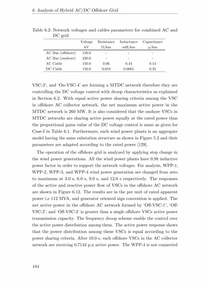
6 Analysis of Hybrid AC/DC Offshore Grid

Table 6.2: Network voltages and cables parameters for combined AC andDC grid

Voltage Resistance Inductance Capacitance

kV Ω/km mH/km µ/km

AC Bus (offshore) 150.0 - - -

AC Bus (onshore) 220.0 - - -

AC Cable 150.0 0.06 0.44 0.14

DC Cable 150.0 0.019 0.0001 0.35

VSC-3’, and ‘On-VSC-4’ are forming a MTDC network therefore they are

controlling the DC voltage control with droop characteristics as explained

in Section 6.2. With equal active power sharing criteria among the VSC

in offshore AC collector network, the net maximum active power in the

MTDC network is 260 MW. It is also considered that the onshore VSCs in

MTDC networks are sharing active power equally at the rated power thus

the proportional gains value of the DC voltage control is same as given for

Case-I in Table 6.1. Furthermore, each wind power plants is an aggregate

model having the same substation structure as shown in Figure 5.2 and their

parameters are adapted according to the rated power [129].

The operation of the offshore grid is analyzed by applying step change in

the wind power generations. All the wind power plants have 0.98 inductive

power factor in order to support the network voltages. For analysis, WPP-1,

WPP-2, WPP-3, and WPP-4 wind power generation are changed from zero

to maximum at 3.0 s, 6.0 s, 9.0 s, and 12.0 s respectively. The responses

of the active and reactive power flow of VSCs in the offshore AC network

are shown in Figure 6.12. The results are in the per unit of rated apparent

power i.e 112 MVA, and generator oriented sign convention is applied. The

net active power in the offshore AC network formed by ‘Off-VSC-1’, ‘Off-

VSC-2’, and ‘Off-VSC-3’ is greater than a single offshore VSCs active power

transmission capacity. The frequency droop scheme enable the control over

the active power distribution among them. The active power response shows

that the power distribution among these VSCs is equal according to the

power sharing criteria. After 10.0 s, each offshore VSCs in the AC collector

network are receiving 0.7143 p.u active power. The WPP-4 is not connected

184

6.3 Integration of Offshore AC and DC Grids

2.0 4.0 6.0 8.0 10.0 12.0 14.0

Time (s)

-1.0

-0.8

-0.6

-0.4

-0.2

0.0

0.2A

ctiv

e P

ow

er (

p.u

)

Off-VSC-1

Off-VSC-2

Off-VSC-3

Off-VSC-4

(a) Active Power Response

2.0 4.0 6.0 8.0 10.0 12.0 14.0

Time (s)

-0.4

-0.3

-0.2

-0.1

0.0

0.1

0.2

0.3

0.4

Rea

ctiv

e P

ow

er (

p.u

)

Off-VSC-1

Off-VSC-2

Off-VSC-3

Off-VSC-4

(b) Reactive Power Response

Figure 6.12: The power response of offshore VSCs.

with the AC collector network thus ‘Off-VSC-4’ is receiving the full wind

power generation i.e 0.9 p.u. Although, wind power plants are absorbing the

reactive power (inductive) from the network, the VSCs in the offshore AC

network requires to flow inductive reactive power as shown in Figure 6.12b.

This is due to the offshore AC cable capacitance which is comparatively

higher than the onshore AC cables. On the other hand, the ‘Off-VSC-4’ is

flowing capacitive reactive power since the AC cable connected with WPP-4

is not long. However, the reactive power can be managed in the offshore AC

network by both offshore wind power plants and VSCs.

The offshore VSCs formed the AC collector network by imposing the

frequencies and controlling the voltages. The response of the offshore VSCs

frequencies and voltages are shown in Figure 6.13. It can be observed that

the offshore AC network frequency is raised above the nominal value at

steady-state. This change in the frequency enable the power distribution

among the offshore VSCs. On the other hand, the frequency imposed by

‘Off-VSC-4’ is constant since there is no other VSC to share the active power.

The energizing of the offshore network is mainly done by controlling the

voltage through VSC outer voltage control. Note that there is lack of inertia

in the offshore AC network since only static devices (only VSCs) exist in

it. Any sudden change in the power imbalance in the network will directly

impact the voltages, and VSCs voltage control has to ensure the network

185

6 Analysis of Hybrid AC/DC Offshore Grid

2.0 4.0 6.0 8.0 10.0 12.0 14.0

Time (s)

0.9997

0.9998

0.9999

1.0000

1.0001

1.0002

1.0003

Fre

qu

ency

(p

.u)

Off-VSC-1

Off-VSC-2

Off-VSC-3

Off-VSC-4

(a) Frequencies Imposed by Offshore VSCs

2.0 4.0 6.0 8.0 10.0 12.0 14.0

Time (s)

0.98

1.00

1.02

1.04

1.06

1.08

1.10

AC

Vo

ltag

e M

agn

itu

de

(p.u

)

Off-VSC-1

Off-VSC-2

Off-VSC-3

Off-VSC-4

2.99 3.00 3.01

1.00

1.02

1.04

3.02

(b) AC Voltages at VSCs Busbars

Figure 6.13: The response of offshore VSCs frequencies and their correspon-ding busbar voltages.

stability. The response of the offshore network AC voltages are shown in

Figure 6.13b. It is clear that the VSC voltage control is robust and the

network voltage reaches to steady-state value fast to ensure network stability

i.e current response settling time is 20 ms. The maximum voltage rise in

the offshore AC network is 1.04 p.u, and the voltage rise due to change in

WPP-4 wind power is approximately 1.10 p.u.

The response of the active power flowing through the onshore VSCs and

the DC voltages at these converters busbars are shown in Figure 6.14. The

‘On-VSC-1’ is injecting approximately 0.7143 p.u active power into the

‘Grid-1’. The active power supply into this grid can only be increased by

altering the power sharing factor of ‘Off-VSC-1’. However, the supply of

active power into other onshore grids can be controlled either by the power

sharing factor within the MTDC network or with the increase in the MTDC

network net power through ‘Off-VSC-2’, and ’Off-VSC-3’ converters. Note

that the frequency droop scheme in the offshore VSCs do not permit the

different active power flow directions with respect to each other. In other

words, all the offshore VSCs will supply the active power into the offshore

AC network to compensate the network losses when there is no wind power

generation. And, they all will receive the active power in case of wind energy

generation. This is evidence from the active power response of Figure 6.12a.

186

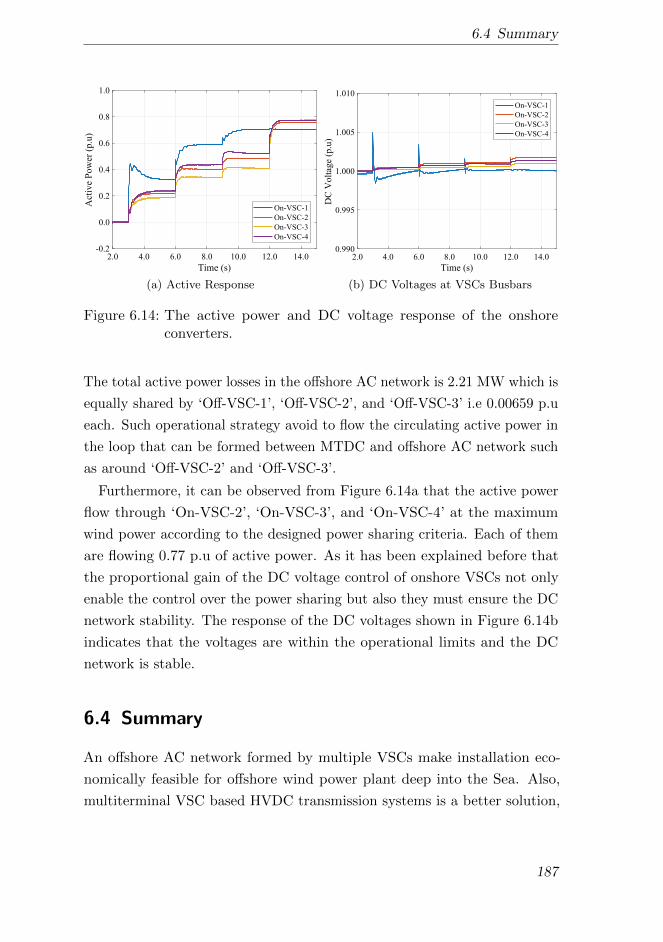
6.4 Summary

2.0 4.0 6.0 8.0 10.0 12.0 14.0

Time (s)

-0.2

0.0

0.2

0.4

0.6

0.8

1.0A

ctiv

e P

ow

er (

p.u

)

On-VSC-1

On-VSC-2

On-VSC-3

On-VSC-4

(a) Active Response

2.0 4.0 6.0 8.0 10.0 12.0 14.0

Time (s)

0.990

0.995

1.000

1.005

1.010

DC

Vo

ltag

e (p

.u)

On-VSC-1

On-VSC-2

On-VSC-3

On-VSC-4

(b) DC Voltages at VSCs Busbars

Figure 6.14: The active power and DC voltage response of the onshoreconverters.

The total active power losses in the offshore AC network is 2.21 MW which is

equally shared by ‘Off-VSC-1’, ‘Off-VSC-2’, and ‘Off-VSC-3’ i.e 0.00659 p.u

each. Such operational strategy avoid to flow the circulating active power in

the loop that can be formed between MTDC and offshore AC network such

as around ‘Off-VSC-2’ and ‘Off-VSC-3’.

Furthermore, it can be observed from Figure 6.14a that the active power

flow through ‘On-VSC-2’, ‘On-VSC-3’, and ‘On-VSC-4’ at the maximum

wind power according to the designed power sharing criteria. Each of them

are flowing 0.77 p.u of active power. As it has been explained before that

the proportional gain of the DC voltage control of onshore VSCs not only

enable the control over the power sharing but also they must ensure the DC

network stability. The response of the DC voltages shown in Figure 6.14b

indicates that the voltages are within the operational limits and the DC

network is stable.

6.4 Summary

An offshore AC network formed by multiple VSCs make installation eco-

nomically feasible for offshore wind power plant deep into the Sea. Also,

multiterminal VSC based HVDC transmission systems is a better solution,

187

6 Analysis of Hybrid AC/DC Offshore Grid

compare to point-to-point configuration, for the trade between the onshore

grids via offshore grid. The DC voltage droop control is a simplest and

effective control scheme to control the MTDC network with multiple onshore

converters, which also enable the control over the power sharing. However,

the trade between onshore grids become difficult using droop control. The

enhancement of the simple droop scheme as a dead-band droop control can

over come this limitation. Further, it is demonstrated that an offshore AC

network formed by connecting several offshore wind power plants using AC

cables interconnection can also be connected with MTDC network with ease.

188

7 Conclusions, Applications, and

Future Works

The overall research findings are summarized in this chapter. The possible

applications and future works have also been highlighted in this chapter.

7.1 Conclusions

The offshore grid has diverse benefits for the transnational electrical network

and future offshore wind power integration. Future offshore grid at North

and Baltic sea would be the combination of AC and DC network. To build

such a network, a gradual approach have to be taken that must utilize the

existing electrical grid infrastructure at offshore and reaches the stage of

fully functional integrated network. In this regard, the aim of this thesis

is to design the control of voltage source converter for high voltage direct

current transmission system to cover the operational aspects of offshore grid.

The different stages of offshore grid evolution have been analyzed started

from point-to-point configuration up to the combined operation of offshore

AC and multiterminal DC network.

In the first stage, the control of the VSC is designed from the prospective of

the HVDC transmission system in point-to-point configuration. In this confi-

guration, the control design establishes the fundamental control structure of

the VSC which consists of inner and outer control system. The inner control

loop is always a current closed loop while the outer control loop depends on

the operational mode such as voltage or power control. The control loops are

cascaded which imply that the reference of the inner control loop is set by the

outer control loop. By this, the control loops can be designed sequentially as

well as extended for network level control. The current closed loop inclusion

189

7 Conclusions, Applications, and Future Works

for both grid synchronous and grid forming mode enables the possibility of

restraining the current flow by controller limits as well as react fast against

any disturbances. This gives an advantage over other schemes of VSC grid

forming control such as direct voltage control. The VSC controller design

method for each operational mode, and the stability conditions for controller

gains selection is addressed in Chapter 2. The chapter also established the

fundamental control structure for offshore, onshore and wind generation unit

substations which has been applied through out the research.

In the second stage of offshore grid development, interconnections of

different wind power plants can be made using HVAC cables and the net

energy can be exported to different onshore grids via VSC-HVDC trans-

mission system in point-to-point configuration. Such a network is formed

by multiple grid forming VSCs operating in parallel. Using frequency and

voltage droop scheme as the VSC network level control, the offshore AC

grid can be operated on the analogue principle of onshore grid with multiple

synchronous machines. The droop gains provide the ability to control the

power distribution among the offshore VSCs which can be set according to

the energy export requirement of the onshore grids. The ability to control

the power distribution is an additional degree of freedom to optimize network

operation for minimizing losses and voltage deviation in the network. Howe-

ver, the application of voltage droop scheme could lead to long term voltage

instability due to reactive power generation by changing VSC controlling

busbar voltage. Thus, the criteria of selecting voltage droop gains has been

developed for better control over reactive power in the offshore AC network

which is presented in Chapter 3.

Apart from the steady-state operation requirement, the frequency and

voltage droop gains must also be selected according to the offshore AC

network stability conditions. By performing small-signal stability analysis,

the stable boundary condition of droop gain can be determined. This study

is presented in Chapter 4. The results suggest that the impact of the droop

gains on the network stability are correlated with the performance of the

VSC. Thus, in order to analyze the complete system stability, the VSC

current and voltage control loops dynamics is essential to be included in

the small-signal modeling of offshore AC network. By analyzing frequency

190

7.1 Conclusions

response using developed model, it has been concluded that the sufficient

damping in the system cannot be achieved at all the high frequencies due to

the performance limitation of the VSC. Although the VSC low-pass filter at

the power measurement may increase damping in the voltage and frequency

response, wind generation units also need to limit the rate of change of

power injection for better system performance.

For long distance energy transmission especially from offshore wind power

plant, the concept of offshore DC hub may have precedence over AC hub but

the lack of DC circuit breaker availability for high DC voltage application

restrains the development of multiterminal HVDC transmission system. On

the other hand, the protection schemes in offshore AC network formed by

multiple grid forming VSCs can be based on the conventional AC circuit

breaker. Since the HVDC transmission system is in point-to-point configura-

tion, the DC fault can be isolated by opening IGBTs and AC circuit breaker.

In the offshore AC network, the selectivity can be ensured using AC circuit

breaker. The fault-ride-through capability is needed in both offshore VSCs

and wind generation units to allow sufficient time for protection devices to

isolate the faulty cable. The short circuit analysis of an offshore AC network

is presented in Chapter 5. The research concludes that the current control in

the VSC grid forming mode enables the direct control over the current during

short circuit to protect the IGBTs, and allow the continue operation in post

fault state after network voltage restored. During fault, the transmission

system VSC switches from voltage control to current control, the voltages

in the network are generated based on the network impedance, and the

current infeed by the VSCs and wind generation units. The magnitude of the

voltage is directly proportional to the fault current, and it is recommended

to inject current with maximum magnitude by VSCs and wind generation

units. Since the voltage phase angle at the VSC controlling busbar is esta-

blished according to the equivalent impedance of the network, the nature of

current infeed either active or reactive depends on the magnitude of the fault

resistance. In order to keep the network stable during fault and post fault

state, it is desirable to keep the voltage phase angle as closed as possible to

its pre-fault state. Usually, the voltage phase angle in the network remains

with in ±π/6 due to stability constraint. For low magnitude fault resistance,

191

7 Conclusions, Applications, and Future Works

the cable series impedance angle is dominant in the equivalent impedance,

hereby requires VSCs to inject capacitive reactive power to keep voltage

phase angle closed to its pre-fault state. On the other hand, it is required

to inject active current for high magnitude fault resistance. The analysis

presents fault behavior of the network at different locations in the offshore

AC network.

Multiple grid forming VSCs provides redundancy in the offshore AC

network and the network can continue to be operated in case of one VSC

failure. In case of malfunction of one ore more grid forming VSCs, the

sum of power infeed by the wind turbine could be greater than the sum

of the combined export capacity of in-operation VSC-HVDC transmission

system. The wind energy is then required to be reduced up to the remaining

export capacity. A frequency coordination control system of VSCs and wind

generation units is developed to reduce the wind generation units power

production without communication signals. The analysis shows that large

transient will appear in the network voltages at the instant of disturbance.

This transient appears due to no inertia in the network and the impacts

of large variation in the power on the network frequency is slower than

on the voltages. The slow reaction of frequency change with respect of

active power delays the process of reducing the wind power consequently

the VSC operational limits is violated. To improve the system response, an

over voltage active current reduction scheme in conjunction of frequency

dependent active current reduction scheme for offshore wind generation units

is proposed. In the proposed scheme, the wind power reduction is made

during initial transient by voltage dependent power reduction scheme later

frequency dependent power reduction scheme supersede and the network

continues to be operated at reduce power with nominal voltages in the

network. The proposed short circuit control scheme is robust and fulfills

the grid code requirements such as FRT, operating split networks, improve

voltage response during fault and post fault state etc.

A MTDC network is preferable solution for the trade between three or

more onshore grids. The formation of offshore AC network can also be

used for energy trade between onshore grids however extra power losses

generated in the offshore converters and cables make the trade process less

192

7.2 Applications

efficient. In Chapter 6, the VSC control scheme is developed for MTDC

network considering the network operational reliability and trade require-

ments. The analysis have shown that the active power distribution in the

MTDC network is possible using DC voltage droop control, and it also

introduced the redundancy of operating MTDC network through multiple

onshore VSCs. The control scheme for onshore VSC for MTDC network

operation is developed with simple modification in the DC voltage control.

For MTDC network operation, all the onshore VSCs have the proportional

control scheme for DC voltage control instead of proportional-plus-integral

control scheme. This has modified the U-I characteristic of VSCs which

now exhibit the principle of DC voltage droop control. A DC optimum

power flow algorithm is developed to determine the DC voltage proportional

controller gains according to the require distribution factor. The DC voltage

control now have to ensure both the stability of the network and trade

requirement. The setting of upper and lower boundary limits for droop gains

in the OPF algorithm by considering the stability limits can provide the

satisfactory solution. Although the DC droop control increase reliability

in the MTDC network, it is difficult to steer power between onshore grids

because of having only one variable (i.e voltage) to control the power both

for balancing and trade. The trade between onshore grids can be improved

by applying dead-band droop characteristics.

As the last stage of the offshore grid development, the thesis presents the

combined operation of the integrated offshore AC and MTDC network.

7.2 Applications

This research can be applied to derive the information and recommendations

for the future wind power plant projects. The results could be useful for

developers, planners and operators as well as to national and international

authorities. The analysis in this research could:

• Assess the information and recommendations for future HVDC trans-

mission systems.

• Beneficial for pre-project planning and realization of offshore wind

193

7 Conclusions, Applications, and Future Works

power plants.

• Demonstrate the possibilities for reliable technical solution for offshore

wind power integration.

• Provide the industry with the open source design tools of VSC based

HVDC transmission system.

• Explore the possibilities for connecting the offshore wind power plants

to the onshore grid, particularly options of an offshore grid extension.

• Provide the tools for optimal operational design of interconnected

offshore and onshore electrical grid, and give insight of its transient

behavior.

The findings of the presented research can be utilized in the definition of

offshore grid codes, and in some of the ongoing European energy projects

such as SuperGrid, MedGrid, Offshore Grid etc.

7.3 Future Works

The concept of an offshore grid is at its earlier state. The presented research

consolidates the key aspects of offshore grids and open up the new ideas in

the said field. Following is a list of ideas that can be considered for future

work.

• In general, the average model of the voltage source converter is sufficient

for power system dynamic and stability analysis. The average model

is usually applied in order to speed up the simulation process. As a

future work, the detailed MMC based VSCs model can be applied

to evaluate the converter performance using proposed VSC control

system design methodology.

• The Real Time Digital Simulator (RTDS) technology has revolutionized

the power system modeling, analysis and control system design. The

RTDS technology enables the testing and analysis of power system

products under simulated condition close to actual system behavior

194

7.3 Future Works

through ‘Power-Hardware in the loop’. The RTDS can be utilized

to model and analyze the hybrid AC/DC offshore grid presented in

the thesis more specifically offshore AC and DC grids, wind farms

generators, converter, and operational control schemes to evaluate the

effectiveness of the proposed control strategies.

• In the thesis, the short circuit analysis and control system for an

offshore grid is proposed for symmetrical three phase balance fault.

The unbalance faults and disturbances in the offshore AC network

can also be analyzed as the future extension of the proposed control

scheme.

• DC fault analysis is another key issue that needs to be addressed for

an offshore AC network that is connected either with MTDC network

or point-to-point VSC-HVDC transmission system.

• Large offshore wind power plants are required to provide the frequency

support to the onshore grids. In the presented control scheme, the

offshore AC network is operated at variable frequency in order to control

the distribution of active power among the transmission system. The

frequency droop gain designing procedure consider that the maximum

over frequency limit must not exceed for all normal operating points i.e

50.2 Hz. Thus, the provision of frequency support by the wind power

plants can be designed above this limit. In this regard, the extension

of the presented control scheme is to incorporate the onshore grid

frequency control scheme with the control of active power distribution

of offshore AC network. Also, the discussion and analysis needs to be

done on; what would be the over frequency limit in the offshore grid

code?

195

196

Appendix A

Author Publications

A.1 Publication in Journals

1. M. Raza, K. Schoenleber, and O. Gomis-Bellmunt, “Droop control

design of multi-VSC system for offshore network to integrate wind

energy” Energies (MDPI), 9(10):826, oct 2016, doi: 10.3390/en9100826.

2. M. Raza, E. Prieto-Araujo, and O. Gomis-Bellmunt, “Small signal

stability analysis of offshore AC network having multiple voltage source

converters” IEEE Transactions on Power Delivery, doi: 10.1109/TP-

WRD.2017.2725982.

3. M. Raza, C. Collados, and O. Gomis-Bellmunt, “Reactive power ma-

nagement in an offshore AC network having multiple voltage source

converters” Applied Energy (Elseiver), 206:793-803, nov 2017. ISSN

0306-2619. doi: 10.1016/j.apenergy.2017.08.182.

4. M. Raza, M. Aragues-Penalba, and O. Gomis-Bellmunt, “Short circuit

analysis of an offshore AC network having multiple VSCs imposing fre-

quency” International Journal of Electrical Power and Energy Systems,

Elseiver (peer-reviewed).

A.2 Publication in Conferences

1. M. Raza, and O. Gomis-Bellmunt, “Dynamic modeling and implemen-

tation of VSC-HVDC system: A grid connected offshore wind farm

application” in Proceedings of the 3rd International Conference on

197

Appendix A Author Publications

Smart Grids and Green IT Systems, (Barcelona, Spain), pp. 53-62,

apr 2014.

2. M. Raza, and O. Gomis-Bellmunt, “Multi infeed control of VSC HVDC

transmission system for offshore wind power plant integration” in 13th

International Workshop on Large-Scale Integration of Wind Power

into Power Systems as well as on Transmission Networks for Offshore

Wind Power Plants, (Berlin), pp. 376-381, nov 2014.

3. M. Raza and O. Gomis-Bellmunt, “Control design strategy to en-

hance the fault ride through capability of VSC-HVDC transmission

system interconnecting offshore wind power plant” in EWEA Annual

Conference and Exhibition 2015, (Paris, France), nov 2015.

4. M. Raza and O. Gomis-Bellmunt, “Control system of voltage source

converter to interconnect offshore AC hub with multiple onshore grids”

in 4th International Conference on Renewable Energy Research and

Application, (Palermo, Italy), nov 2015.

5. M. Raza, C. Collados, and O. Gomis-Bellmunt, “Reactive power ma-

nagement in an offshore AC network having multiple voltage source

converters” in 16th IEEE International Conference on Environment

and Electrical Engineering, Florence, Italy, 7-10 jun 2016.

A.3 Publication in Book

1. M. Raza, “Load flow calculation and its application” in PowerFactory

Applications for Power System Analysis SE - 1 (F. M. Gonzalez-

Longatt and J. Luis Rueda, eds.), Power Systems, pp. 1-25, Springer

International Publishing, 2014.

198

Appendix B

Mathematics for VSC System

B.1 Per Unit System for Network Parameters

Usually, it is convenient to design the control and perform the analysis in per

unit (p.u) system. It simplify the computational process by eliminating the

units. The base values for the principle variables are selected such that they

are equal to one per unit under rated condition. For the network parameters,

the base value of power and voltage are defined while current and impedance

base values are calculated using ohm laws.

With the definition of the base power, frequency, and three phase AC

voltage, the base of AC current can be calculated using (B.1). The subscript

b is the notation of base variable.

sb = pb = qb =√

3ubib

ib =sb√3ub

(B.1)

Here, ub is the rated line-to-line RMS voltage, ib is the rated line RMS

current, sb is the base apparent power, pb is the base active power, and qb is

the base reactive power. The base values of the impedance and admittances

can be calculated using (B.2).

zb =u2b

sb, yb =

1

zb(B.2)

Also, the base values of inductance and capacitance are calculated using

(B.3). The resistance base value is equal to the zb.

199

Appendix B Mathematics for VSC System

lb =zbωb, cb =

ybωb

(B.3)

Here, ωb = 2πfb is the network angular frequency base value. Similarly,

the base value for DC network variables can be calculated by defining DC

active power and voltage base values. The DC quantities are notated using

capitalized letter. The base value of current and resistance can then be

calculated using (B.4). Usually, the DC base power is defined equal to the

AC base power.

Ib =PbUb, Rb =

UbIb

(B.4)

B.2 Per Unit System for VSC Control

The three phase voltages and currents are the measurement quantities in the

VSC control system. The Clark transformation matrix given in Chapter 2

preserve the peak of the measurement quantities, in another words it is

called as voltage and current invariant transformation. In phasor notation,

the measured three phase balanced voltage and current can be written as

(B.5) in αβ0 frame.

uαβ0 pu(t) = Um puej(ωt+δ), iαβ0 pu(t) = Im pue

j(ωt+ψ), (B.5)

Here, Um pu and Im pu are the peak voltages and current in per unit, δ is

the voltage phase angle, ψ is the current phase angle, and ω is the network

frequency. The complex power is calculated using (B.6) for analytical

analysis. As explained in previous section, the base values are selected so

that the measured signals are equal to 1.0 p.u at the rated values. Thus

for the measurement signals, the base values are rated peak voltage of

line-to-ground voltage (ub =√

2/3ULL) and the rated peak line current

(ib =√

2ILL).

spu(t) = uαβ0 pu(t) · i∗αβ0 pu(t)

spu = Um puIm puej(δ−ψ)

(B.6)

200

B.2 Per Unit System for VSC Control

Let us compare the power calculation using per unit quantity with the

actual value calculation. The matrices for signal transformation into αβ0

frame and its inverse is given in (B.7).

Tαβ0 =2

3

1 −12 −1

2

0√

32 −

√3

212

12

12

, T−1αβ0 =

1 0 1

−12

√3

2 1

−12 −

√3

2 1

(B.7)

The instantaneous three phase power can be calculated as (B.8) using

three phase voltage and current measurement in matrix representation.

s(t) = uTabc(t)iabc(t) =[ua(t) ub(t) uc(t)

]ia(t)ib(t)

ic(t)

(B.8)

By applying the Clark transformation principle on the voltage and current,

the power equation yield as (B.9).

s(t) =(T−1αβ0 · uαβ0(t)

)T· T−1

αβ0 · iαβ0(t)

s(t) = uTαβ0(t) ·(T−1αβ0

)T· T−1

αβ0 · iαβ0(t)

(T−1αβ0

)T· T−1

αβ0 =

32 0 0

0 32 0

0 0 3

(B.9)

First two components are orthogonal in which α component is align with

the a-phase and β components is lagging by −π/2. Third component of

three phase voltage and current is zero in αβ0 frame for the balanced system,

therefore the third component of power is also zero. Thus, power, voltage

and current can be written in instantaneous vector form as expressed by

(B.10). Note that the quantities are in actual values.

s =3

2uαβ0(t) · i∗αβ0(t)

uαβ0(t) = uα(t) + juβ(t), iαβ0(t) = iα(t) + jiβ(t)(B.10)

Further, it can be observed from (B.6) that the calculation of power will

201

Appendix B Mathematics for VSC System

become the time invariant function after the product of voltage and current

in αβ0 frame. Thus, power equation can be written in Cartesian coordinate

representation as

P =3

2(uαiα + uβiβ)

Q =3

2(uβiα − uαiβ)

(B.11)

Substitute the actual voltage and current values in (B.10) with the per

unit variables and base values as given in (B.12). It can be observed that the

factor of 3/2 is not required to calculate the power when using measurement

signals in per unit.

s =3√

2√

2

2√

3ULL · ILL · uαβ0 pu(t) · i∗αβ0 pu(t)

s =√

3ULL · ILL · uαβ0 pu(t) · i∗αβ0 pu(t)

spu = uαβ0 pu(t) · i∗αβ0 pu(t)

(B.12)

Normally, the small signal analysis or control system design methods

are performed using actual quantities of the variables. These analysis and

methods provide the controller gains in units of actual quantities. For the

control system implementation in per unit system, these controller gains

need to be converted appropriately. In the presented thesis, the controller

gains that are designed for VSC is belong to either one of the three main

control systems i.e inner, outer, and network level controller.

The inner control is the current control loops in which input is current

and output signal is voltage. Thus, the unit of inner current controller gains

is V/A, and the actual controller gain value must be divided by the AC

impedance base value for per unit control system.

The outer controller gains unit depends on the control loop. For active

and reactive power control loop, the controller gains are unit less since the

per unit absolute value of power and current are same in dq0 frame. For

AC voltage control in both grid forming and grid synchronous mode, the

output of the controller is the current and input is voltage ergo the controller

gain unit is A/V and the gains must be multiplied by the AC impedance

202

B.2 Per Unit System for VSC Control

base value for per unit control implementation. For DC voltage control, the

input is DC voltage and output is the current which makes its unit as A/V

therefore DC base resistance needs to be multiplied with the controller gains

to set in per unit control system.

The network level control mainly consists of frequency and voltage droop

control. The unit of voltage droop gain is V/Var and the factor that needs

to multiply with the voltage droop value is sb/ub. Similarly, the unit of

frequency droop gain is Hz/W and the gain is multiplied with the factor

calculated as sb/ωb. Note that the droop gain value determined by the OPF

algorithm is in per unit variables, and they are not required to be converted.

203

204

Bibliography

[1] Nathalie Girouard, Elianna Konialis, Cecilia Tam, and Peter Taylor.

Energy. OECD Green Growth Studies. OECD Publishing, jan 2012.

ISBN 9789264115101. doi: 10.1787/9789264115118-en.

[2] Mihai Tomescu, Ils Moorkens, Wouter Wetzels, Lukas Emele, Hannah

Foerster, and Benjamin Greiner. Renewable energy in Europe 2016:

Recent growth and knock-on effects. Technical report, European

Envirnoment Agency, mar 2016. doi: 10.2800/6803.

[3] Daniel Fraile, Giorgio Corbetta, and Ivan Pineda. Making transition

work. Technical report, Wind Europe, sep 2016. URL https://

windeurope.org/.

[4] Ivan Pineda and Pierre Tardieu. Wind in power: 2016 European

statistics. Technical report, Wind Europe, feb 2017. URL https:

//windeurope.org/.

[5] Ivan Pineda and Pierre Tardieu. The European offshore wind industry:

key trends and statistics 2016. Technical report, Wind Europe, jan

2017. URL https://windeurope.org/.

[6] European council 23/24 october 2014 - conclusion: 2030 climate and

energy policy framework, oct 2014. URL https://ec.europa.eu/

clima/policies/strategies/2030_en.

[7] Ayla Uslu. Europe onshore and offshore wind energy potential.

Technical report, European Environment Agency, jun 2009. doi:

10.2800/11373.

[8] Athanasia Arapogianni and Anne Benedicte Genachte. Deep wa-

ter: The next step for offshore wind energy. Technical report,

205

Bibliography

WindEurope, jul 2013. URL https://windeurope.org/about-wind/

reports//deep-water/.

[9] Nicolas Fichaux and Justin Wilkes. Oceans of opportunity. harnessing

Europe’s largest domestic energy resource. Technical report, European

Wind Energy Association, sept 2009. URL http://www.ewea.org/

policy-issues/offshore/.

[10] Stijn Cole, Karim Karoui, Til Kristian Vrana, Olav Bjarte Fosso,

Jean Baptiste Curis, Anne Marie Denis, and Chen Ching Liu. A

European supergrid: Present state and future challenges. In Power

Systems Computation Conference (PSCC). ETH Zurich, aug 2011.

[11] Jan De Decker, Paul Kreutzkamp, Achim Woyte, and Carlos Dierckx-

sens. The impact of large scale offshore electricity transmission: the

European project offshore grid. In 2012 9th International Conference

on the European Energy Market. IEEE, may 2012. ISBN 978-1-4673-

0833-5. doi: 10.1109/EEM.2012.6254680.

[12] WWF. Threats: Effects of climate change, 2017. URL https://www.

worldwildlife.org/threats/effects-of-climate-change. Acces-

sed on 30-05-2017.

[13] MEDOW. Multi terminal DC grid for offshore wind, 2017. URL

http://sites.cardiff.ac.uk/medow/. Accessed on 30-05-2017.

[14] Nikolas Flourentzou, Vassilios Georgios Agelidis, and Georgios Deme-

triades. VSC-Based HVDC power transmission systems: An overview.

IEEE Transactions on Power Electronics, 24(3):592–602, mar 2009.

ISSN 0885-8993. doi: 10.1109/TPEL.2008.2008441.

[15] Fujin Deng and Zhe Chen. Design of protective inductors for HVDC

transmission line within DC grid offshore wind farms. IEEE Tran-

sactions on Power Delivery, 28(1):75–83, jan 2013. ISSN 0885-8977.

doi: 10.1109/TPWRD.2012.2224384.

[16] Ataollah Mokhberdoran, Helder Leite, Adriano Carvalho, and Nuno

Silva. A review on HVDC circuit breakers. In 3rd Renewable Power

206

Bibliography

Generation Conference (RPG 2014). IET, sep 2014. ISBN 978-1-84919-

917-9. doi: 10.1049/cp.2014.0859.

[17] Robert Sellick and Markus Akerberg. Comparison of HVDC light

(VSC) and HVDC classic (LCC) site aspects, for a 500MW 400kV

HVDC transmission scheme. In 10th IET International Conference on

AC and DC Power Transmission (ACDC 2012). IET, dec 2012. ISBN

978-1-84919-700-7. doi: 10.1049/cp.2012.1945.

[18] Mike Barnes. VSC-HVDC Newsletter. University of Manchester, UK,

5(4), apr 2017.

[19] Jeroen Brouwers. Tennet News: TenneT presents Hub and Spoke

concept for large scale wind energy on the North Sea, jun 2016.

URL https://www.tennet.eu/news/detail/tennet-presents-

hub-and-spoke-concept-for-large-scale-wind-energy-on-

the-north-sea/. Accessed on 23-06-2017.

[20] Jeroen Brouwers. Tennet News: Three TSOs sign agreement

on North Sea wind power hub, mar 2017. URL https:

//www.tennet.eu/news/detail/three-tsos-sign-agreement-

on-north-sea-wind-power-hub/. Accessed on 23-06-2017.

[21] Paola Bresesti, Wil Kling, Ralph Hendriks, and Riccardo Vailati.

HVDC connection of offshore wind farms to the transmission system.

IEEE Transactions on Energy Conversion, 22(1):37–43, mar 2007.

ISSN 0885-8969. doi: 10.1109/TEC.2006.889624.

[22] Peter Sandeberg, Paul Moran, Alessio Lomardi, Alvaro Hernan-

dez Manchola, Christian Feltes, and Douglas Ramsay. Special consi-

derations for AC collector systems and substations associated with

HVDC connected wind power plants. Technical Report WG SC B3.36,

CIGRE International Council on Large Electric Systems, mar 2015.

[23] Christof Humpert. Long distance transmission systems for the future

electricity supply: Analysis of possibilities and restrictions. Energy,

207

Bibliography

48(1):278–283, dec 2012. ISSN 03605442. doi: 10.1016/j.energy.2012.

06.018.

[24] Joseph Song Manguelle, Maja Harfman Todorovic, Song Chi, Satish

Gunturi, and Rajib Datta. Power transfer capability of HVAC cables

for subsea transmission and distribution systems. IEEE Transactions

on Industry Applications, 50(4):2382–2391, jul 2014. ISSN 0093-9994.

doi: 10.1109/TIA.2013.2291934.

[25] Wang Xifan, Cao Chengjun, and Zhou Zhichao. Experiment on

fractional frequency transmission system. IEEE Transactions on

Power Systems, 21(1):372–377, feb 2006. ISSN 0885-8950. doi:

10.1109/TPWRS.2005.860923.

[26] Nan Qin, Shi You, Zhao Xu, and Vladislav Akhmatov. Offshore wind

farm connection with low frequency AC transmission technology. In

2009 IEEE Power and Energy Society General Meeting. IEEE, jul

2009. ISBN 978-1-4244-4241-6. doi: 10.1109/PES.2009.5275262.

[27] Jose Luis Dominguez Garcia, Daniel Rogers, Carlos Ernesto

Ugalde Loo, Jun Liang, and Oriol Gomis Bellmunt. Effect of non-

standard operating frequencies on the economic cost of offshore AC

networks. Renewable Energy, 44:267–280, aug 2012. ISSN 09601481.

doi: 10.1016/j.renene.2012.01.093.

[28] Qingrui Tu, Zheng Xu, and Lie Xu. Reduced switching frequency

modulation and circulating current suppression for modular multilevel

converters. IEEE Transactions on Power Delivery, 26(3):2009–2017,

jul 2011. ISSN 0885-8977. doi: 10.1109/TPWRD.2011.2115258.

[29] Weixing Lin, Dragan Jovcic, Samuel Nguefeu, and Hani Saad. Full

bridge MMC converter optimal design to HVDC operational require-

ments. IEEE Transactions on Power Delivery, 31(3):1342–1350, jun

2016. ISSN 0885-8977. doi: 10.1109/TPWRD.2015.2475130.

[30] Jakob Glasdam, Jesper Hjerrild, Lukasz Hubert Kocewiak, and

Claus Leth Bak. Review on multi-level voltage source converter based

208

Bibliography

HVDC technologies for grid connection of large offshore wind farms.

In 2012 IEEE International Conference on Power System Techno-

logy (POWERCON). IEEE, oct 2012. ISBN 978-1-4673-2868-5. doi:

10.1109/PowerCon.2012.6401377.

[31] Michal Sztykiel, Rodrigo da Silva, Remus Teodorescu, Lorenzo Zeni,

Lars Helle, and Philip Carne Kjaer. Modular multilevel converter

modelling, control and analysis under grid frequency deviations. In

2013 15th European Conference on Power Electronics and Applications

(EPE). IEEE, sep 2013. ISBN 978-1-4799-0116-6. doi: 10.1109/EPE.

2013.6634747.

[32] Lidong Zhang, Hans Peter Nee, and Lennart Harnefors. Analysis of

stability limitations of a VSC HVDC link using power synchronization

control. IEEE Transactions on Power Systems, 26(3):1326–1337, aug

2011. ISSN 0885-8950. doi: 10.1109/TPWRS.2010.2085052.

[33] Wenyuan Wang, Antony Beddard, Mike Barnes, and Ognjen Mar-

janovic. Analysis of active power control for VSC HVDC. IEEE

Transactions on Power Delivery, 29(4):1978–1988, aug 2014. ISSN

0885-8977. doi: 10.1109/TPWRD.2014.2322498.

[34] Manuel Reyes, Pedro Rodriguez, Sergio Vazquez, Alvaro Luna, Remus

Teodorescu, and Juan Manuel Carrasco. Enhanced decoupled double

synchronous reference frame current controller for unbalanced grid

voltage conditions. IEEE Transactions on Power Electronics, 27(9):

3934–3943, sep 2012. ISSN 0885-8993. doi: 10.1109/TPEL.2012.

2190147.

[35] Jiabing Hu and Ziqiang Zhu. Improved voltage vector sequences on

dead beat predictive direct power control of reversible three phase

grid connected voltage source converters. IEEE Transactions on

Power Electronics, 28(1):254–267, jan 2013. ISSN 0885-8993. doi:

10.1109/TPEL.2012.2194512.

[36] Mehrdad Yazdanian and Ali Mehrizi Sani. Internal model based

current control of the RL filter based voltage sourced converter. IEEE

209

Bibliography

Transactions on Energy Conversion, 29(4):873–881, dec 2014. ISSN

0885-8969. doi: 10.1109/TEC.2014.2353035.

[37] Salvatore D’Arco, Jon Are Suul, and Olav Bjarte Fosso. Small signal

modeling and parametric sensitivity of a virtual synchronous machine

in islanded operation. International Journal of Electrical Power and

Energy Systems, 72:3–15, mar 2015. ISSN 01420615. doi: 10.1016/j.

ijepes.2015.02.005.

[38] Michael Bierhoff and Friedrich Wilhelm Fuchs. Active damping for

three phase PWM rectifiers with high order line side filters. IEEE

Transactions on Industrial Electronics, 56(2):371–379, feb 2009. ISSN

0278-0046. doi: 10.1109/TIE.2008.2007950.

[39] Aleksandr Reznik, Marcelo Godoy Simoes, and Ahmed Al-Durra. LCL

filter design and performance analysis for grid interconnected systems.

IEEE Transactions on Industry Applications, 50(2):1225–1232, mar

2014. ISSN 0093-9994. doi: 10.1109/TIA.2013.2274612.

[40] Fei Li, Xing Zhang, Hong Zhu, Haoyuan Li, and Changzhou Yu. An

LCL-LC filter for grid connected converter: Topology, parameter and

analysis. IEEE Transactions on Power Electronics, 30(9):5067–5077,

sep 2014. ISSN 0885-8993. doi: 10.1109/TPEL.2014.2367135.

[41] Dragan Jovcic, Lu Zhang, and Masood Hajian. LCL VSC Converter

for high power applications. IEEE Transactions on Power Delivery,

28(1):137–144, jan 2013. ISSN 0885-8977. doi: 10.1109/TPWRD.2012.

2219560.

[42] Remus Beres, Xiongfei Wang, Frede Blaabjerg, Claus Leth Bak, and

Marco Liserre. A review of passive filters for grid connected voltage

source converters. In 2014 IEEE Applied Power Electronics Conference

and Exposition, pages 2208–2215. IEEE, mar 2014. ISBN 978-1-4799-

2325-0. doi: 10.1109/APEC.2014.6803611.

[43] Bozo Terzic, Goran Majic, and Alojz Slutej. Stability analysis of

three phase PWM converter with LCL filter by means of nonlinear

210

Bibliography

model. Journal for Control, Measurement, Electronics, Computing and

Communications (AUTOMATIKA), 51(3):221–232, sep 2010. ISSN

00051144.

[44] Antony Beddard and Mike Barnes. AC fault ride through of MMC

VSC HVDC systems. In 7th IET International Conference on Power

Electronics, Machines and Drives (PEMD 2014). IET, apr 2014. ISBN

978-1-84919-815-8. doi: 10.1049/cp.2014.0382.

[45] Yan Liu and Zhe Chen. A flexible power control method of VSC HVDC

link for the enhancement of effective short circuit ratio in a hybrid

multi infeed HVDC system. IEEE Transactions on Power Systems,

28(2):1568–1581, may 2013. ISSN 0885-8950. doi: 10.1109/TPWRS.

2012.2222057.

[46] Osman Addalan Kalcon Giddani, Abdelaziz Yousif Mohamed Abbas,

Grain P. Adam, Olimpo Anaya Lara, and Kwok Lun Lo. Multi task

control for VSC HVDC power and frequency control. International

Journal of Electrical Power and Energy Systems, 53:684–690, dec 2013.

ISSN 01420615. doi: 10.1016/j.ijepes.2013.05.002.

[47] Tennet TSO GmbH. Requirements for offshore grid con-

nections in the grid of TenneT TSO GmbH, dec 2012.

URL http://www.tennet.eu/de/en/customers/grid-customers/

grid-connection-regulations.html.

[48] Tennet TSO GmbH. Grid code, high and extra high voltage,

dec 2012. URL http://www.tennet.eu/de/en/customers/grid-

customers/grid-connection-regulations.html.

[49] Arjen van der Meer, Mario Ndreko, Madeleine Gibescu, and Mart

van der Meijden. The effect of FRT behavior of VSC HVDC connected

offshore wind power plants on AC/DC system dynamics. IEEE Tran-

sactions on Power Delivery, 31(2):878–887, apr 2016. ISSN 0885-8977.

doi: 10.1109/TPWRD.2015.2442512.

211

Bibliography

[50] Agusti Egea Alvarez, Jef Beerten, Dirk Van Hertem, and Oriol Go-

mis Bellmunt. Primary and secondary power control of multiterminal

HVDC grids. In 10th IET International Conference on AC and DC

Power Transmission (ACDC 2012). Institution of Engineering and

Technology, dec 2012. doi: 10.1049/cp.2012.1989.

[51] Christian Feltes, Holger Wrede, Friedrich Koch, and Istvan Erlich.

Enhanced fault ride through method for wind farms connected to the

grid through VSC based HVDC transmission. IEEE Transactions

on Power Systems, 24(3):1537–1546, aug 2009. ISSN 0885-8950. doi:

10.1109/TPWRS.2009.2023264.

[52] Francisco Gonzalez Longatt. Optimal steady state operation of a

MTDC system based on DC independent system operator objectives. In

11th IET International Conference on AC and DC Power Transmission.

IET, feb 2015. ISBN 978-1-84919-982-7. doi: 10.1049/cp.2015.0031.

[53] Eduardo Prieto Araujo, Agusti Egea Alvarez, Sajjad Fekri, and Oriol

Gomis Bellmunt. DC voltage droop control design for multi-terminal

HVDC systems considering AC and DC grid dynamics. IEEE Tran-

sactions on Power Delivery, 31(2):575–585, apr 2016. ISSN 0885-8977.

doi: 10.1109/TPWRD.2015.2451531.

[54] Giddani Kalcon, Grain Philip Adam, Olimpo Anaya Lara, Stephen

Lo, and Kjetil Uhlen. Small signal stability analysis of multi-terminal

VSC-based DC transmission systems. IEEE Transactions on Power

Systems, 27(4):1818–1830, nov 2012. ISSN 08858950. doi: 10.1109/

TPWRS.2012.2190531.

[55] Lie Xu and Liangzhong Yao. DC voltage control and power dispatch

of a multi terminal HVDC system for integrating large offshore wind

farms. IET Renewable Power Generation, 5(3):223, may 2011. ISSN

17521416. doi: 10.1049/iet-rpg.2010.0118.

[56] Zhuo di Wang, Ke Jun Li, Jing guo Ren, Li Jun Sun, Jian Guo Zhao,

Yong Liang Liang, Wei Jen Lee, Zhao hao Ding, and Ying Sun. A

coordination control strategy of voltage source converter based MTDC

212

Bibliography

for offshore wind farms. IEEE Transactions on Industry Applications,

51(4):2743–2752, jul 2015. ISSN 0093-9994. doi: 10.1109/TIA.2015.

2407325.

[57] Wenyuan Wang and Mike Barnes. Power flow algorithms for multi

terminal VSC HVDC with droop control. IEEE Transactions on

Power Systems, 29(4):1721–1730, jul 2014. ISSN 0885-8950. doi:

10.1109/TPWRS.2013.2294198.

[58] Rodrigo Teixeira-pinto. Multi-terminal DC network: System integra-

tion, dynamics and control. PhD thesis, Delft University of Technology,

2014.

[59] Jef Beerten, Stijn Cole, and Ronnie Belmans. Generalized steady

state VSC MTDC model for sequential AC/DC power flow algorithms.

IEEE Transactions on Power Systems, 27(2):821–829, may 2012. ISSN

0885-8950. doi: 10.1109/TPWRS.2011.2177867.

[60] Monica Aragues-Penalba, Agusti Egea-Alvarez, Samuel Galceran Arel-

lano, and Oriol Gomis Bellmunt. Droop control for loss minimization

in HVDC multi-terminal transmission systems for large offshore wind

farms. Electric Power Systems Research, 112:48–55, jul 2014. ISSN

03787796. doi: 10.1016/j.epsr.2014.03.013.

[61] Wang Feng, Anh Le Tuan, Lina Bertling Tjernberg, Anders Mannikoff,

and Anders Bergman. A new approach for benefit evaluation of multi-

terminal VSC HVDC using a proposed mixed AC and DC optimal

power flow. IEEE Transactions on Power Delivery, 29(1):432–443, feb

2014. ISSN 0885-8977. doi: 10.1109/TPWRD.2013.2267056.

[62] Roger Wiget and Goeran Andersson. Optimal power flow for combined

AC and multi-terminal HVDC grids based on VSC converters. In 2012

IEEE Power and Energy Society General Meeting. IEEE, jul 2012.

ISBN 978-1-4673-2729-9. doi: 10.1109/PESGM.2012.6345448.

[63] Lianxiang Tang and Boon Teck Ooi. Locating and isolating DC faults

in multi-terminal DC systems. IEEE Transactions on Power Delivery,

213

Bibliography

22(3):1877–1884, jul 2007. ISSN 0885-8977. doi: 10.1109/TPWRD.

2007.899276.

[64] Bernardo Silva, Carlos Leal Moreira, Helder Leite, and Joao Pecas

Lopes. Control strategies for AC fault ride through in multi-terminal

HVDC grids. IEEE Transactions on Power Delivery, 29(1):395–405,

feb 2014. ISSN 0885-8977. doi: 10.1109/TPWRD.2013.2281331.

[65] Oriol Gomis Bellmunt, Jun Liang, Janaka Ekanayake, Rosemary King,

and Nicholas Jenkins. Topologies of multiterminal HVDC VSC trans-

mission for large offshore wind farms. Electric Power Systems Research,

81:271–281, feb 2011. ISSN 03787796. doi: 10.1016/j.epsr.2010.09.006.

[66] Hanchao Liu and Jian Sun. Voltage stability and control of offshore

wind farms with AC collection and HVDC transmission. IEEE Journal

of Emerging and Selected Topics in Power Electronics, 2(4):1181–1189,

dec 2014. ISSN 2168-6777. doi: 10.1109/JESTPE.2014.2361290.

[67] Telles Brunelli Lazzarin, Guilherme Bauer, and Ivo Barbi. A control

strategy for parallel operation of single phase voltage source inverters:

analysis, design, and experimental results. IEEE Transactions on

Industrial Electronics, 60(6):2194–2204, jun 2013. ISSN 0278-0046.

doi: 10.1109/TIE.2012.2193856.

[68] Wanderley Alves Parreira, Henrique Jose Avelar, Joao Batista Vieira,

Luiz Carlos Freitas, Luiz Carlos Gomes de Freitas, and Ernane Anto-

nio Alves Coelho. Small signal analysis of parallel connected voltage

source inverters using a frequency and voltage droop control inclu-

ding an additional phase shift. Journal of Control, Automation and

Electrical Systems, 25(5):597–607, oct 2014. ISSN 2195-3880. doi:

10.1007/s40313-014-0143-5.

[69] Ernane Antonio Alves Coelho, Porfirio Cabaleiro Cortizo, and Pedro

Francisco Donoso Garcia. Small signal stability for parallel connected

inverters in stand alone AC supply systems. IEEE Transactions on

Industry Applications, 38(2):533–542, mar 2002. ISSN 00939994. doi:

10.1109/28.993176.

214

Bibliography

[70] Charles Sao and Peter Lehn. Autonomous load sharing of voltage

source converters. IEEE Transactions on Power Delivery, 20(2):1009–

1016, apr 2005. ISSN 0885-8977. doi: 10.1109/TPWRD.2004.838638.

[71] Karel De Brabandere, Bruno Bolsens, Jeroen Van den Keybus, Achim

Woyte, Johan Driesen, and Ronnie Belmans. A voltage and frequency

droop control method for parallel inverters. IEEE Transactions on

Power Electronics, 22(4):1107–1115, jul 2007. ISSN 0885-8993. doi:

10.1109/TPEL.2007.900456.

[72] Hisham Mahmood, Dennis Michaelson, and Jin Jiang. Accurate

reactive power sharing in an islanded microgrid using adaptive virtual

impedances. IEEE Transactions on Power Electronics, 30(3):1605–

1617, mar 2015. ISSN 0885-8993. doi: 10.1109/TPEL.2014.2314721.

[73] Yixin Zhu, Fang Zhuo, Feng Wang, Baoquan Liu, and Yangjie Zhao.

A wireless load sharing strategy for islanded microgrid based on feeder

current sensing. IEEE Transactions on Power Electronics, 30(12):6706–

6719, dec 2015. ISSN 0885-8993. doi: 10.1109/TPEL.2014.2386851.

[74] Martin Andreasson, Roger Wiget, Dimos Dimarogonas, Karl Johans-

son, and Goran Andersson. Distributed primary frequency control

through multi-terminal HVDC transmission systems. In 2015 Ame-

rican Control Conference (ACC), pages 5029–5034. IEEE, jul 2015.

ISBN 978-1-4799-8684-2. doi: 10.1109/ACC.2015.7172122.

[75] Samy Akkari, Marc Petit, Jing Dai, and Xavier Guillaud. Inte-

raction between the voltage droop and the frequency droop control

for multi-terminal HVDC systems. IET Generation, Transmission

and Distribution, 10(6):1345–1352, apr 2016. ISSN 1751-8687. doi:

10.1049/iet-gtd.2015.0814.

[76] Jiebei Zhu, Campbell Booth, Grain Philip Adam, and Andrew Roscoe.

Inertia emulation control of VSC-HVDC transmission system. In 2011

International Conference on Advanced Power System Automation and

Protection, volume 1. IEEE, oct 2011. ISBN 978-1-4244-9621-1. doi:

10.1109/APAP.2011.6180514.

215

Bibliography

[77] Xiaobo Hu, Jun Liang, Daniel Rogers, and Yalou Li. Power flow and

power reduction control using variable frequency of offshore AC grids.

IEEE Transactions on Power Systems, 28(4):3897–3905, nov 2013.

ISSN 0885-8950. doi: 10.1109/TPWRS.2013.2257884.

[78] Ahmed Moawwad, Mohamed Shawky El Moursi, and Weidong Xiao.

A novel transient control strategy for VSC-HVDC connecting offshore

wind power plant. IEEE Transactions on Sustainable Energy, 5(4):1056–

1069, oct 2014. ISSN 1949-3029. doi: 10.1109/TSTE.2014.2325951.

[79] Istvan Erlich, Fekadu Shewarega, Christian Feltes, Friedrich Koch,

and Jens Fortmann. Offshore wind power generation technologies.

Proceedings of the IEEE, 101(4):891–905, apr 2013. ISSN 0018-9219.

doi: 10.1109/JPROC.2012.2225591.

[80] Zhe Chen and Hui Li. Overview of different wind generator systems and

their comparisons. IET Renewable Power Generation, 2(2):123–138,

jun 2008. ISSN 1752-1416. doi: 10.1049/iet-rpg:20070044.

[81] Mario Ndreko, Marjan Popov, and Mart van der Meijden. Study on

FRT compliance of VSC-HVDC connected offshore wind plants during

AC faults including requirements for the negative sequence current

control. International Journal of Electrical Power and Energy Systems,

85:97–116, feb 2017. ISSN 01420615. doi: 10.1016/j.ijepes.2016.08.009.

[82] Omer Goksu, Remus Teodorescu, Claus Leth Bak, Florin Iov, and

Philip Carne Kjaer. Instability of wind turbine converters during

current injection to low voltage grid faults and PLL frequency based

stability solution. IEEE Transactions on Power Systems, 29(4):1683–

1691, jul 2014. ISSN 0885-8950. doi: 10.1109/TPWRS.2013.2295261.

[83] Bernd Weise. Impact of K-factor and active current reduction during

fault ride through of generating units connected via voltage sourced con-

verters on power system stability. IET Renewable Power Generation,

9(1):25–36, jan 2015. ISSN 1752-1416. doi: 10.1049/iet-rpg.2014.0116.

216

Bibliography

[84] Reigh Walling, Ekrem Gursoy, and Bruce English. Current contributi-

ons from Type 3 and Type 4 wind turbine generators during faults.

In 2011 IEEE Power and Energy Society General Meeting. IEEE, jul

2011. ISBN 978-1-4577-1000-1. doi: 10.1109/PES.2011.6039740.

[85] Tobias Neumann, Thomas Wijnhoven, Geert Deconinck, and Istvan Er-

lich. Enhanced dynamic voltage control of Type 4 wind turbines during

unbalanced grid faults. IEEE Transactions on Energy Conversion, 30

(4):1650–1659, 2015. ISSN 0885-8969. doi: 10.1109/TEC.2015.2470126.

[86] Istvan Erlich, Worawat Nakawiro, and Marcela Martinez Rojas. Opti-

mal dispatch of reactive sources in wind farms. In 2011 IEEE Power

and Energy Society General Meeting. IEEE, jul 2011. ISBN 978-1-

4577-1000-1. doi: 10.1109/PES.2011.6039534.

[87] Monica Alonso, Hortensia Amaris, and Carlos Alvarez Ortega. A

multiobjective approach for reactive power planning in networks with

wind power generation. Renewable Energy, 37(1):180–191, jan 2012.

ISSN 09601481. doi: 10.1016/j.renene.2011.06.021.

[88] Marcela Martinez Rojas, Andreas Sumper, Oriol Gomis Bellmunt, and

Antoni Sudria Andreu. Reactive power dispatch in wind farms using

particle swarm optimization technique and feasible solutions search.

Applied Energy, 88(12):4678–4686, dec 2011. ISSN 03062619. doi:

10.1016/j.apenergy.2011.06.010.

[89] Hoan Van Pham, Jose Luis Rueda, and Istvan Erlich. Online optimal

control of reactive sources in wind power plants. IEEE Transactions

on Sustainable Energy, 5(2):608–616, apr 2014. ISSN 1949-3029. doi:

10.1109/TSTE.2013.2272586.

[90] Jan De Deckar and Paul Kreutzkamp. Offshore electricity grid

infrastructure in Europe: A techno-economic assessment. Techni-

cal report, OffshoreGrid (3E Coordinator), oct 2011. URL http:

//www.offshoregrid.eu/.

217

Bibliography

[91] Ebrahim Rokrok and Mohamad Esmail Hamedani Golshan. Adaptive

voltage droop scheme for voltage source converters in an islanded

multibus microgrid. IET Generation, Transmission and Distribution,

4(5):562–578(16), may 2010. ISSN 17518687. doi: 10.1049/iet-gtd.

2009.0146.

[92] Donghwan Kim, Kyosun Jung, Kyungbae Lim, and Jaeho Choi. A

droop method for high capacity parallel inverters considering accurate

real power sharing. Journal of Power Electronics, 16(1):38–47, jan

2016. ISSN 1598-2092. doi: 10.6113/JPE.2016.16.1.38.

[93] Ngoc Tuan Trinh, Marcus Zeller, Klaus Wuerflinger, and Istvan Erlich.

Generic model of MMC VSC HVDC for interaction study with AC

power system. IEEE Transactions on Power Systems, 31(1):27–34, jan

2016. ISSN 0885-8950. doi: 10.1109/TPWRS.2015.2390416.

[94] Se Kyo Chung. A phase tracking system for three phase utility interface

inverters. IEEE Transactions on Power Electronics, 15(3):431–438,

may 2000. ISSN 08858993. doi: 10.1109/63.844502.

[95] Lus Guilherme Barbosa Rolim, Diogo Rodrigues da Costa, and Maurcio

Aredes. Analysis and software implementation of a robust synchro-

nizing PLL circuit based on the PQ theory. IEEE Transactions on

Industrial Electronics, 53(6):1919–1926, dec 2006. ISSN 0278-0046.

doi: 10.1109/TIE.2006.885483.

[96] XiaoQiang Guo, WeiYang Wu, and HeRong Gu. Phase locked loop

and synchronization methods for grid-interfaced converters: a review.

Przeglad Elektrotechniczny, 87(4), jan 2011. ISSN 0033-2097.

[97] Dunstan Graham and R. C. Lathrop. The synthesis of optimum

transient response: Criteria and standard forms. Transactions of the

American Institute of Electrical Engineers, Part II: Applications and

Industry, 72(5):273–288, nov 1953. ISSN 0097-2185. doi: 10.1109/TAI.

1953.6371346.

218

Bibliography

[98] Ivan Pineda, Kristian Ruby, Andrew Ho, Ariola Mbistrova, and Giorgio

Corbetta. The European offshore wind inductry: key trends and statis-

tics 1st half 2016. Technical report, European Wind Energy Associa-

tion, jul 2016. URL http://www.ewea.org/statistics/offshore/.

[99] Sascha Thorsten Schroder, Peter Meibom, Stephan Spiecker, and

Christoph Weber. Market impact of an offshore grid: A case study.

In 2010 IEEE Power and Energy Society General Meeting. IEEE, jul

2010. ISBN 978-1-4244-6549-1. doi: 10.1109/PES.2010.5590044.

[100] Jan De Decker, Jens Tambke, Jakob Voelker, and Katarzyna Micha-

lowska Knap. An offshore transmission grid for wind power integration:

The European techno-economic study offshore grid. In IEEE Power

and Energy Society General Meeting. IEEE, jul 2010. ISBN 978-1-

4244-6549-1. doi: 10.1109/PES.2010.5589887.

[101] Abbas Rabiee, Maziar Vanouni, and Mostafa Parniani. Optimal

reactive power dispatch for improving voltage stability margin using a

local voltage stability index. Energy Conversion and Management, 59:

66–73, jul 2012. ISSN 01968904. doi: 10.1016/j.enconman.2012.02.017.

[102] ABB. Product Catalog: XLPE submarine cable systems,

2017. URL http://new.abb.com/cables/cables/hvac-extruded-

cables/hvac-submarine-cables.

[103] Nexans. Product catalog: Nexans submarine power cables, 2013. URL

http://www.nexans.de.

[104] Giorgio Chiandussi, Marco Codegone, Simone Ferrero, and Federico Er-

minio Varesio. Comparison of multi objective optimization metho-

dologies for engineering applications. Computers and Mathematics

with Applications, 63(5):912–942, mar 2012. ISSN 08981221. doi:

10.1016/j.camwa.2011.11.057.

[105] Federal Ministry for Economic Affairs, Energy (BMWi), and Project

Executing Organization (PTJ). Wind speed data: FINO databank,

2017. URL http://fino.bsh.de/. Accessed on 23-03-2017.

219

Bibliography

[106] ENERCON. Product catalog: ENERCON product overview, 2017.

URL http://www.enercon.de/en/home/. Accessed on 23-03-2017.

[107] Amirnaser Yazdani and Iravani Reza. Voltage Control. In Voltage

sourced converters in power systems: Modeling, control, and applica-

tions, chapter Controlled frequency VSC system. A John Wiley and

Son, 2010. ISBN 9780470521564.

[108] Luis Fernando Costa Alberto and Newton Geraldo Bretas. Estimating

the frequencies of load buses and their effects on the critical clearing

time. In 1998 International Conference on Power System Technology

(POWERCON 98), volume 2, pages 1310–1314. IEEE, aug 1998. ISBN

0-7803-4754-4. doi: 10.1109/ICPST.1998.729298.

[109] Mohammad Hassanzahraee and Alireza Bakhshai. Transient droop

control strategy for parallel operation of voltage source converters

in an islanded mode microgrid. In 2011 IEEE 33rd International

Telecommunications Energy Conference (INTELEC). IEEE, oct 2011.

ISBN 9781457712494. doi: 10.1109/INTLEC.2011.6099827.

[110] Nkt-Cables. Product Catalog: High voltage cable system- cables and

accessories up to 550 kV, 2017. URL www2.nktcables.com.

[111] Janusz Bialek. European offshore power grid demonstration projects.

In 2012 IEEE Power and Energy Society General Meeting. IEEE, jul

2012. ISBN 978-1-4673-2729-9. doi: 10.1109/PESGM.2012.6345283.

[112] Mario Ndreko, Ana-Maria Bucurenciu, Marjan Popov, and Mart

van der Meijden. On grid code compliance of offshore MTDC grids:

modeling and analysis. In 2015 IEEE Eindhoven PowerTech. IEEE,

jun 2015. ISBN 978-1-4799-7693-5. doi: 10.1109/PTC.2015.7232398.

[113] Istvan Erlich, Christian Feltes, and Fekadu Shewarega. Enhanced

voltage drop control by VSC HVDC systems for improving wind farm

fault ride through capability. IEEE Transactions on Power Delivery,

29(1):378–385, feb 2014. ISSN 0885-8977. doi: 10.1109/TPWRD.2013.

2285236.

220

Bibliography

[114] Jorun Irene Marvik and Harald Georg Svendsen. Analysis of grid

faults in offshore wind farm with HVDC connection. Energy Procedia,

35:81–90, jan 2013. ISSN 18766102. doi: 10.1016/j.egypro.2013.07.161.

[115] Monica Aragues Penalba, Oriol Gomis Bellmunt, and Marcia Martins.

Coordinated control for an offshore wind power plant to provide fault

ride through capability. IEEE Transactions on Sustainable Energy, 5

(4):1253–1261, oct 2014. ISSN 1949-3029. doi: 10.1109/TSTE.2014.

2344172.

[116] Sungduck Kim, Medhat Morcos, and Juan Carlos Gomez. Voltage

sag magnitude and phase jump due to short circuits in distribution

systems with variable fault resistance. Electric Power Components and

Systems, 33(5):493–512, aug 2005. doi: 10.1080/15325000590504984.

[117] Istvan Erlich, Fekadu Shewarega, Stephan Engelhardt, Jorg Kret-

schmann, Jens Fortmann, and Friedrich Koch. Effect of wind tur-

bine output current during faults on grid voltage and the transient

stability of wind parks. In 2009 IEEE Power and Energy Society

General Meeting. IEEE, jul 2009. ISBN 978-1-4244-4241-6. doi:

10.1109/PES.2009.5275626.

[118] Peter Fairley. Germany jump-starts the Supergrid: New developements

in high voltage DC electronics could herald an epic shift energy delivery.

IEEE spectrum, may 2013. ISSN 0018-9235.

[119] Hakan Ergun, Dirk Van Hertem, and Ronnie Belmans. Transmission

system topology optimization for large scale offshore wind integration.

IEEE transactions on sustainable energy, 3(4):908–917, oct 2012. ISSN

1949-3037. doi: 10.1109/TSTE.2012.2199341.

[120] Stefano Lauria, Marco Maccioni, Francesco Palone, and Maddalena

Schembari. Very long distance connection of gigawatt size offshore wind

farms: Extra high voltage AC versus high voltage DC cost comparison.

IET Renewable Power Generation, 10(5):713–720, may 2016. ISSN

1752-1416. doi: 10.1049/iet-rpg.2015.0348.

221

Bibliography

[121] Bjorn Gustavsen and Olve Mo. Variable transmission voltage for loss

minimization in long offshore wind farm AC export cables. IEEE

Transactions on Power Delivery, 32(3):1422–1431, jun 2017. ISSN

0885-8977. doi: 10.1109/TPWRD.2016.2581879.

[122] Rodrigo Teixeira Pinto, Christian Alejandro, Monica Aragues Penalba,

Andreas Sumper, and Elmer Sorrentino. A fast methodology for solving

power flows in hybrid AC/DC networks: The European North Sea

Supergrid case study. In PCIM Europe 2016; International Exhibition

and Conference for Power Electronics, Intelligent Motion, Renewable

Energy and Energy Management, pages 2211–2218. VDE, may 2016.

ISBN 9783800741861.

[123] Yunhui Huang, Xiaoming Yuan, Jiabing Hu, Pian Zhou, and Dong

Wang. DC bus voltage control stability affected by AC bus voltage

control in VSCs connected to weak AC grids. IEEE Journal of Emer-

ging and Selected Topics in Power Electronics, 4(2):445–458, jun 2016.

ISSN 2168-6777. doi: 10.1109/JESTPE.2015.2480859.

[124] Roberto Sandano, Michael Farrell, and Malabika Basu. Enhanced

master slave control strategy enabling grid support services and offshore

wind power dispatch in a multi terminal VSC HVDC transmission

system. Renewable Energy, 113:1580–1588, dec 2017. ISSN 0960-1481.

doi: 10.1016/J.RENENE.2017.07.028.

[125] Haifeng Li, Chongru Liu, Gengyin Li, and Reza Iravani. An enhanced

DC voltage droop control for the VSC HVDC grid. IEEE Transactions

on Power Systems, 32(2):1520–1527, mar 2017. ISSN 0885-8950. doi:

10.1109/TPWRS.2016.2576901.

[126] Pierre Rault, Frederic Colas, Xavier Guillaud, and Samuel Nguefeu.

Method for small signal stability analysis of VSC-MTDC grids. In

2012 IEEE Power and Energy Society General Meeting. IEEE, jul

2012. ISBN 978-1-4673-2729-9. doi: 10.1109/PESGM.2012.6345318.

[127] Catalin Gavriluta, Ignacio Candela, Alvaro Luna, Antonio Gomez-

Exposito, and Pedro Rodriguez. Hierarchical control of HV MTDC

222

Bibliography

systems with droop based primary and OPF based secondary. IEEE

Transactions on Smart Grid, 6(3):1502–1510, may 2015. ISSN 1949-

3053. doi: 10.1109/TSG.2014.2365854.

[128] Florian Thams, Robert Eriksson, and Marta Molinas. Interaction of

droop control structures and its inherent effect on the power transfer

limits in multiterminal VSC HVDC. IEEE Transactions on Power

Delivery, 32(1):182–192, feb 2017. ISSN 0885-8977. doi: 10.1109/

TPWRD.2016.2600028.

[129] James Conroy and Ronald William Watson. Aggregate modelling of

wind farms containing full-converter wind turbine generators with per-

manent magnet synchronous machines: transient stability studies. IET

Renewable Power Generation, 3(1):39–52, mar 2009. ISSN 17521416.

doi: 10.1049/iet-rpg:20070091.

223