Off-policy TD(λ) with a true online equivalence

Hado van Hasselt A. Rupam MahmoodReinforcement Learning and Artificial Intelligence Laboratory

University of Alberta, Edmonton, AB T6G 2E8 Canada

Richard S. Sutton

Abstract

Van Seijen and Sutton (2014) recently proposeda new version of the linear TD(λ) learning algo-rithm that is exactly equivalent to an online for-ward view and that empirically performed bet-ter than its classical counterpart in both predic-tion and control problems. However, their al-gorithm is restricted to on-policy learning. Inthe more general case of off-policy learning, inwhich the policy whose outcome is predicted andthe policy used to generate data may be differ-ent, their algorithm cannot be applied. One rea-son for this is that the algorithm bootstraps andthus is subject to instability problems when func-tion approximation is used. A second reasontrue online TD(λ) cannot be used for off-policylearning is that the off-policy case requires so-phisticated importance sampling in its eligibilitytraces. To address these limitations, we gener-alize their equivalence result and use this gen-eralization to construct the first online algorithmto be exactly equivalent to an off-policy forwardview. We show this algorithm, named true on-line GTD(λ), empirically outperforms GTD(λ)(Maei, 2011) which was derived from the sameobjective as our forward view but lacks the ex-act online equivalence. In the general theoremthat allows us to derive this new algorithm, weencounter a new general eligibility-trace update.

1 Temporal difference learning

Eligibility traces improve learning in temporal-difference(TD) algorithms by efficiently propagating credit for laterobservations back to update earlier predictions (Sutton,1988), and can help speed up learning significantly. A goodway to interpret these traces, the extent of which is reg-ulated by a trace parameter λ ∈ [0, 1], is to consider theeventual updates to each prediction. For λ = 1 the up-

date for the prediction at time t is similar to a Monte Carloupdate towards the full return following t. For λ = 0 theprediction is updated toward only the immediately (reward)signal, and the rest of the return is estimated with the pre-diction at the next state. Such an interpretation is calleda forward view, because it considers the effect of futureobservations on the updates. In practice, learning is oftenfastest for intermediate values of λ (Sutton & Barto, 1998).

Traditionally, the equivalence to a forward view was knownto hold only when the predictions are updated offline. Inpractice TD algorithms are more commonly used online,during learning, but then this equivalence was only approx-imate. Recently, van Seijen and Sutton (2014) developedtrue online TD(λ), the first algorithm to be exactly equiv-alent to a forward view under online updating. For λ = 1the updates by true online TD(λ) eventually become ex-actly equivalent to a Monte Carlo update towards the fullreturn. As demonstrated by van Seijen and Sutton, such anonline equivalence is more than a theoretical curiosity, andleads to lower prediction errors than when using the tradi-tional TD(λ) algorithm that only achieves an offline equiv-alence. In this paper, we generalize this result and showexact online equivalences are possible for a wide range offorward views, leading to computationally efficient onlinealgorithms by exploiting a new generic trace update.

A limitation of the true online TD(λ) algorithm by vanSeijen and Sutton (2014) is that it is only applicable to on-policy learning, when the learned predictions correspondto the policy that is used to generate the data. Off-policylearning is important to be able to learn from demonstra-tions, to learn about many things at the same time (Suttonet al., 2011), and ultimately to learn about the unknown op-timal policy. A natural next step is therefore to apply ourgeneral equivalence result to an off-policy forward view.We construct such a forward view and derive an equivalentnew off-policy gradient TD algorithm, that we call true on-line GTD(λ). This algorithm is constructed to be equivalentfor λ = 0, by design, to the existing GTD(λ) algorithm(Maei, 2011). We demonstrate empirically that for higherλ the new algorithm is much better behaved due to its exact

equivalence to a desired forward view. In addition to thepractical potential of the new algorithm, this demonstratesthe usefulness of our general equivalence result and the re-sulting new trace update.

2 Problem setting

We consider a learning agent in an unknown environmentwhere at each time step t the agent performs an action Atafter which the environment transitions from the currentstate St to the next state St+1. We do not assume the stateitself can be observed and the agent instead observes a fea-ture vector φt ∈ Rn, which is typically a function of thestate St such that φt

.= φ(St). The agent selects its actions

according to a behavior policy b, such that b(a|St) denotesthe probability of selecting action At = a in state St. Typ-ically b(a|s) depends on s through φ(s).

After performing At, the agent observes a scalar (reward)signal Rt+1 and the process can either terminate or con-tinue. We allow for soft terminations, defined by a po-tentially time-varying state-dependent termination factorγt ∈ [0, 1] (cf. Sutton, Mahmood, Precup & van Hasselt,2014). With weight 1 − γt+1 the process terminates attime t + 1 and Rt+1 is considered the last reward in thisepisode. With weight γt+1 we continue to the next stateand observe φt+1

.= φ(St+1). The agent then selects a

new action At+1 and this process repeats. A special case isthe episodic setting where γt = 1 for all non-terminatingtimes t and γT = 0 when the episode ends at time T . Thetermination factors are commonly called discount factors,because they discount the effect of later rewards.

The goal is to predict the sum of future rewards, discountedby the probabilities of termination, under a target policy π.The optimal prediction is thus defined for each state s by

vπ(s).= Eπ

[ ∞∑t=1

Rt

t−1∏k=1

γk | S0 = s

],

where Eπ[ · ] .= E[ · | At ∼ π(·|St),∀t ] is the expectancyconditional on the policy π. We estimate the values vπ(s)with a parameterized function of the observed features. Inparticular we consider linear functions of the features, suchthat θ>t φt ≈ vπ(St) is the estimated value of the state attime t according to a weight vector θt. The goal is then toimprove the predictions by updating θt.

We desire online algorithms with a constant O(n) per-stepcomplexity, where n is the number of features in φ. Suchcomputational considerations are important in settings witha lot of data or when φt is a large vector. For instance, wewant our algorithms to be able to run on a robot with manysensors and limited on-board processing power.

3 General online equivalence betweenforward and backward views

We can think about what the ideal update would be for aprediction after observing all relevant future rewards andstates. Such an update is called a forward view, because itdepends on observations from the future. A concrete ex-ample is the on-policy Monte Carlo return, consisting ofthe discounted sum of all future rewards.

In practice, full Monte Carlo updates can have high vari-ance. It can be better to augment the return with the then-current predictions at the visited states. When we con-tinue after some time step t, with weight γt+1, we replacea portion of 1 − λt+1 of the remaining return with ourcurrent prediction of this return at St+1. Making use oflater predictions to update earlier predictions in this wayis called bootstrapping. The process then continues to thenext action and reward with total weight γt+1λt+1, whereagain we terminate with 1 − γt+2 and then bootstrap with1 − λt+2, and so on. When λt+1 = 0 we get the usualone-step TD return Rt+1 + γt+1φ

>t+1θt. If λt = 1 for

all t, we obtain a full (discounted) Monte Carlo return. Inthe on-policy setting, when we do not have to worry aboutdeviations from the target policy, we can then update theprediction made at time t towards the on-policy λ-returndefined by

Gλt = Rt+1 + γt+1

[(1− λt+1)φ>t+1θt + λt+1G

λt+1

].

The discount factors γt are normally considered a propertyof the problem, but the bootstrap parameters λt can be con-sidered tunable parameters. The full return (obtained forλ = 1) is an unbiased estimate for the value of the be-havior policy, but its variance can be high. The value es-timates are typically not unbiased, but can be considerablyless variable. As such, one can interpret the λ parameters astrading off bias and variance. Typically, learning is fastestfor intermediate values of λ.

If termination never occurs, Gλt is never fully defined. Toconstruct a well-defined forward view, we can truncate therecursion at the current data horizon (van Seijen & Sutton,2014; Sutton et al., 2014) to obtain interim λ-returns. If wehave data up to time t, all returns are truncated as if λt = 0and we bootstrap on the most recent value estimateφ>t θt−1of the current state. This gives us, for each 0 ≤ k < t

Gλk,t = Rk+1 + γk+1

[(1− λk+1)φ>k+1θk + λk+1G

λk+1,t

]and Gλt,t = φ>t θt−1. In this definition of Gλk,t, for eachtime step j with k < j ≤ t the value of state Sj is estimatedusing φ>j θj−1, because θj−1 is the most up-to-date weightvector at the moment we reach this state.

Using these interim returns, we can construct an interimforward view which, in contrast to conventional forward

views, can be computed before an episode has concludedor even if the episode never fully terminates. For instance,when we have data up to time t the following set of linearupdates for all times k < t is an interim forward view:

θtk+1 = θtk + αk(Gλk,t − φ>k θtk)φk , k < t , (1)

where θt0.= θ0 is the initial weight vector. The subscript

on θtk (first index on Gλk,t) corresponds to the state for thekth update, the superscript (second index on Gλk,t) denotesthe current data horizon.

The forward view (1) is well-defined and computable atevery time t, but it is not very computationally efficient.For each new observation, when t increments to t + 1, wepotentially have to recompute all the updates, as Gλk,t+1

might differ from Gλk,t for arbitrary many k. The resultingcomputational complexity is O(nt) per time step, whichis problematic when t becomes large. Therefore, forwardviews are not meant to be implemented as is. They serve asa conceptual update, in which we formulate what we wantto achieve after observing the relevant data.

In the next theorem, we prove that for many forward viewsan efficient and fully equivalent backward view exists thatexploits eligibility traces to construct online updates thatuse only O(n) computation per time step, but that still re-sult in exactly the same weight vectors. The theorem isconstructive, allowing us to find such backward views au-tomatically for a given forward view.

Theorem 1 (Equivalence between forward and backwardviews). Consider any forward view that updates towardssome interim targets Y tk with

θtk+1 = θtk + ηk(Y tk − φ>k θtk)φk + xk , 0 ≤ k < t ,

where θt0 = θ0 for some initial θ0 and where xk ∈ Rnis any vector that does not depend on t. Assume that thetemporal differences Y t+1

k − Y tk for different k are relatedthrough

Y t+1k − Y tk = ck(Y t+1

k+1 − Ytk+1) , ∀k < t , (2)

where ck is a scalar that does not depend on t. Then, thefinal weights θtt at each t are equal to the weights θt asdefined by e0 = η0φ0 and the backward view

θt+1 = θt + (Y t+1t −Y tt )et + ηt(Y

tt −φ>t θt)φt + xt ,

et = ct−1et−1 + ηt(1− ct−1φ>t et−1)φt , t > 0 . (3)

Proof. We introduce the fading matrix Ft.= I − ηtφtφ>t ,

such that θtk+1 = Fkθtk + ηkY

tkφk. We subtract θtt from

θt+1t+1 to find the change when t increments. Expanding

θt+1t+1 , we get

θt+1t+1 − θtt

= Ftθt+1t − θtt + ηtY

t+1t φt + xt

= Ft(θt+1t − θtt) + ηtY

t+1t φt + (Ft − I)θtt + xt

= Ft(θt+1t − θtt) + ηtY

t+1t φt − ηtφtφ>t θtt + xt

= Ft(θt+1t − θtt) + ηt(Y

t+1t − φ>t θtt)φt + xt . (4)

We now repeatedly expand both θt+1t and θtt to get

θt+1t − θtt

= Ft−1(θt+1t−1 − θtt−1) + ηt−1(Y t+1

t−1 − Y tt−1)φt−1

= Ft−1Ft−2(θt+1t−1 − θtt−1)

+ ηt−2(Y t+1t−2 − Y tt−2)Ft−1φt−2

+ ηt−1(Y t+1t−1 − Y tt−1)φt−1

= . . . (Expand until reaching θt+10 − θt0 = 0.)

= Ft−1 · · ·F0(θt+10 − θt0)

+

t−1∑k=0

ηkFt−1· · ·Fk+1(Y t+1k − Y tk )φk

=

t−1∑k=0

ηkFt−1· · ·Fk+1(Y t+1k − Y tk )φk

=

t−1∑k=0

ηkFt−1· · ·Fk+1ck(Y t+1k+1 − Y

tk+1)φk (Using (2))

= . . . (Apply (2) repeatedly.)

= ct−1

t−1∑k=0

ηk

t−2∏j=k

cj

Ft−1· · ·Fk+1φk︸ ︷︷ ︸.= et−1

(Y t+1t − Y tt )

= ct−1et−1(Y t+1t − Y tt ) . (5)

The vector et can be computed with the recursion

et =

t∑k=0

ηk

t−1∏j=k

cj

Ft · · ·Fk+1φk

=

t−1∑k=0

ηk

t−1∏j=k

cj

Ft · · ·Fk+1φk + ηtφt

= ct−1Ft

t−1∑k=0

ηk

t−2∏j=k

cj

Ft−1 · · ·Fk+1φk + ηtφt

= ct−1Ftet−1 + ηtφt

= ct−1et−1 + ηt(1− ct−1φ>t et−1)φt .

We plug (5) back into (4) and obtain

θt+1t+1 − θtt

= ct−1Ftet−1(Y t+1t − Y tt ) + ηt(Y

t+1t − φ>t θt)φt + xt

= (et − ηtφt)(Y t+1t − Y tt ) + ηt(Y

t+1t − φ>t θt)φt + xt

= (Y t+1t − Y tt )et + ηt(Y

tt − φ>t θt)φt + xt .

Because θ0,t.= θ0 for all t, the desired result follows

through induction.

The theorem shows that under condition (2) we can turn ageneral forward view into an equivalent online algorithmthat only uses O(n) computation per time step. Comparedto previous work on forward/backward equivalences, thisgrants us two important things. First, the obtained equiva-lence is both online and exact; most previous equivalenceswere only exact under offline updating, when the weightsare not updated during learning (Sutton & Barto, 1998;Sutton et al., 2014). Second, the theorem is constructive,and gives an equivalent backward view directly from a de-sired forward view, rather than having to prove such anequivalence in hindsight (as in, e.g., van Seijen & Sutton,2014). This is perhaps the main benefit of the theorem:rather than relying on insight and intuition to construct effi-cient online algorithms, Theorem 1 can be used to derive anexact backward view directly from a desired forward view.We exploit this in Section 6 when we turn a desired off-policy forward view into an efficient new online off-policyalgorithm.

We refer to traces of the general form (3) as dutch traces.The trace update can be interpreted as first shrinking thetraces with c, for instance c = γλ, and then updating thetraces for the current state, φ>e, towards one with a stepsize of η. In contrast, traditional accumulating traces, de-fined by et = ct−1et−1 + φt, add to the trace value of thecurrent state rather than updating it toward one. This cancause the accumulating traces to grow large, potentially re-sulting in high-variance updates.

To demonstrate one advantage of Theorem 1, we apply itto the on-policy TD(λ) forward view defined by (1).

Theorem 2 (Equivalence for true online TD(λ)). Defineθt0 = θ0. Then, θtt as defined by (1) equals θt as definedby the backward view

δt = Rt+1 + γφ>t+1θt − φ>t θt−1 ,et = γλet−1 + αt(1− γλφ>t et−1)φt ,

θt+1 = θt + δtet + αt(φ>t θt−1 − φ>t θt)φt .

Proof. In Theorem 1, we substitute xt = 0, ct = γλ andY tk = Gλk,t, such that Y t+1

t − Y tt = δt and Y tt = φ>t θt−1.The desired result follows immediately.

The backward view in Theorem 2 is true online TD(λ), asproposed by van Seijen and Sutton (2014). Using The-orem 1, we have proved equivalence to its forward viewwith a few simple substitutions, whereas the original proofis much longer and more complex.

4 Off-policy learning

In this section, we turn to off-policy learning with functionapproximation. In constructing an off-policy forward viewtwo issues arise that are not present in the on-policy set-ting. First, we need to estimate the value of a policy thatis different than the one used to obtain the observations.Second, using a forward view such as (1) under off-policysampling can cause it to be unstable, potentially resultingin divergence of the weights (Sutton et al., 2008). Theseissues can be avoided by constructing our off-policy algo-rithms to minimize a mean-squared projected Bellman er-ror (MSPBE) with gradient descent (Sutton et al., 2009;Maei & Sutton, 2010; Maei, 2011).

The MSPBE was previously used to derive GTD(λ) (Maei,2011), which is an online algorithm that can be used tolearn off-policy predictions. GTD(λ) was not constructedto be exactly equivalent to any forward view and it is anatural question whether the algorithm can be improvedfrom having such an equivalence, just as was the case withTD(λ) and true online TD(λ). In this section, we introducean off-policy MSPBE and show how GTD(λ) can be de-rived. In the next section, we use the same MSPBE to con-struct a new off-policy forward view from which we willderive an exactly equivalent online backward view.

To obtain estimates for one distribution when the samplesare generated under another distribution, we can weight theobservations by the relative probabilities of these observa-tions occurring under the target policy, as compared to thebehavior distribution. This is called importance sampling(Rubinstein, 1981; Precup, Sutton & Singh, 2000). Re-call that b(a|s) and π(a|s) denote the probabilities of se-lecting action a in state s according to the behavior policyand the target policy, respectively. After selecting an ac-tion At in a state St according to b, we observe a rewardRt+1. The expected value of this reward is Eb[Rt+1], but ifwe multiply the reward with the importance-sampling ratioρt

.= π(At|St)/b(At|St) the expected value is

Eb[ρtRt+1|St] =∑a

b(a|St)π(a|St)b(a|St)

E[Rt+1 | St, At = a]

=∑a

π(a|St)E[Rt+1 | St, At = a]

= Eπ[Rt+1 | St] .

Therefore ρtRt+1 is an unbiased sample for the rewardunder the target policy. This technique can be applied toall the rewards and value estimates in a given λ-return.

For instance, if we want to obtain an unbiased sample forthe reward under the target policy n steps after the cur-rent state St, the total weight applied to this reward shouldbe ρtρt+1 · · · ρt+n−1. An off-policy λ-return starting fromstate St is given by

Gλρt (θ) = ρt

(Rt+1 + γk+1(1− λk+1)φ>k+1θ (6)

+ γk+1λk+1Gλk+1(θ)

).

In contrast to Gλt , this return is defined as a function of asingle weight vector θ. This is useful later, when we wishto determine the gradient of this return with respect to θ.

When using function approximation it is generally not pos-sible to estimate the value of each state with full accu-racy or, equivalently, to reduce the conditional expectedTD error for each state to zero at the same time. Moreformally, let vθ be a parameterized value function definedby vθ(s) = θ>φ(s) and let Tλπ be a parametrized Bellmanoperator defined, for any v : {s} → R, by

(Tλπ v)(s) =

Eπ[R1 + γ1(1− λ1)v(S1) + γ1λ1(Tλπ v)(S1) | S0 = s

].

In general, we then cannot achieve vθ = Tλπ vθ, becauseTλπ vθ is not guaranteed to be a function that we can rep-resent with our chosen function approximation. It is, how-ever, possible to find the fixed point defined by

vθ = ΠTλπ vθ . (7)

where Πv is a projection of v into the space of representablefunctions {vθ | θ ∈ Rn}. Let d be the steady-state distri-bution of states under the behavior policy. The projectionof any v is then defined by

Πv = vθv , where θv = arg minθ

‖vθ − v‖2d ,

where ‖ · ‖2d is a norm defined by ‖f‖2d.=∑s d(s)f(s)2.

Following Maei (2011), the projection is definedin terms of the steady-state distribution result-ing from the behavior policy, which means thatd(s) = limt→∞ P(St = s | Aj ∼ b(·|Sj),∀j). Thisimplies our objective weights the importance of theaccuracy of the prediction in each state according to therelative frequency that this state occurs under the behaviorpolicy, which is a natural choice for online learning.

The fixed point in (7) can be found by minimizing theMSPBE defined by (Maei, 2011)

J(θ) = ‖vθ −ΠTλπ vθ‖2d (8)

= Eb[δπk (θ)φk]>Eb

[φkφ

>k

]−1 Eb[δπk (θ)φk] ,

where δπk (θ).= (Tλπ vθ)(Sk) − vθ(Sk) and where the ex-

pectancies are with respect to the steady-state distribution

d, as induced by the behavior policy b. The ideal gradientupdate for time step k is then

θk+1 = θk −1

2α∇θ J(θ)|θk , (9)

where

− 1

2∇θ J(θ)|θk

= −Eb[∇θδπk (θ)φ>k

]Eb[φkφ

>k

]−1 Eb[δπk (θk)φk]

= Eb[(φk −∇θGλρk (θ))φ>k

]Eb[φkφ

>k

]−1Eb[δπk (θk)φk]

= Eb[δπk (θk)φk]

− Eb[∇θGλρk (θ)φ>k

]Eb[φkφ

>k

]−1 Eb[δπk (θk)φk]

= Eb[δπk (θk)φk]− Eb[∇θGλρk (θ)φk

]>w∗ , (10)

with Gλρk as defined in (6), and where

w∗.= Eb

[φkφ

>k

]−1 Eb[δπk (θk)φk] .

Update (9) can be interpreted as an expected forward view.

The derivation of the GTD(λ) algorithm proceeds by ex-ploiting the expected equivalences (Maei, 2011)

Eb[∇θGk(θ)φ>k

]= Eb

[ρkγk+1(1− λk+1)φk+1φ

>k

]+ Eb

[ρkγk+1λk+1∇θGk+1(θ)φ>k

]= Eb

[ρkγk+1(1− λk+1)φk+1φ

>k

]+ Eb

[ρk−1γkλk∇θGk(θ)φ>k−1

]= Eb

[ρkγk+1(1− λk+1)φk+1φ

>k

]+ Eb

[ρk−1γkλkρkγk+1(1− λk+1)φk+1φ

>k−1]

+ Eb[ρk−1γkλkρkγk+1λk+1∇θGk+1(θ)φ>k−1

]= Eb

[ρkγk+1(1− λk+1)φk+1φ

>k

]+ Eb

[ρk−1γkλkρkγk+1(1− λk+1)φk+1φ

>k−1]

+ Eb[ρk−2γk−1λk−1ρk−1γkλk∇θGk(θ)φ>k−2

]= . . . (Repeat until we reach φ0.)

= Eb[γk+1(1− λk+1)φk+1 ρk

k∑j=0

k∏i=j+1

ρi−1γiλi

φ>j︸ ︷︷ ︸.= (e∇k )>

]

= Eb[γk+1(1− λk+1)φk+1(e∇k )>

], (11)

and, similarly, Eb[δπk (θk)φk] = Eb[δk(θk)e∇k ], where

e∇t = ρt(γtλte∇t−1 + φt) , (12)

δt(θ) = Rt+1 + γt+1φ>t+1θ − φ>t θ .

The auxiliary vector wt ≈ w∗ can be updated with leastmean squares (LMS) (Sutton et al., 2009; Maei, 2011), us-ing the sample δt(θt)e∇t ≈ Eb[δt(θt)e∇t ] = Eb[δπt (θt)φt]

and the update

wt+1 = wt + βtδt(θt)e∇t − βtφ>t wtφt .

The complete GTD(λ) algorithm is then defined by1

δt = Rt+1 + γt+1φ>t+1θt − φ>t θt ,

e∇t = ρt(γtλte∇t−1 + φt) ,

θt+1 = θt + αtδte∇t − αtγt+1(1− λt+1)w>t e

∇t φt+1 ,

wt+1 = wt + βtδte∇t − βtφ>t wtφt .

5 An off-policy forward view

In this section, we define an off-policy forward view whichwe turn into a fully equivalent backward view in the nextsection, using Theorem 1. GTD(λ) is derived by first turn-ing an expected forward view into an expected backwardview, and then sampling. We propose instead to samplethe expected forward view directly and then invert the sam-pled forward view into an equivalent online backward view.This way we obtain an exact equivalence between forwardand backward views instead of the expected equivalence ofGTD(λ). This was previously not known to be possible, butit has the advantage that we can use the precise (potentiallydiscounted and bootstrapped) sample returns consisting ofall future rewards and state values in each update. This canresult in more accurate predictions, as confirmed by our ex-periments in Section 7.

The new forward view derives from the MSPBE, as definedin (8), and more specifically from the gradient update de-fined by (9) and (10). To find an implementable interimforward view, we need sampled estimates of all three partsin (10). We discuss each of these parts separately.

Our interim forward view is defined in terms of a datahorizon t, so the gradient of the MSPBE is taken to θtkrather than θk. Furthermore, δπk is defined as the errorbetween a λ-return and a current estimate, and thereforewe need to construct an interim λ-return. To estimatethe first term of (10) we therefore need an estimate forEb[δπk (θtk)φk] = Eb[Gλρk,t − φ>k θtk], for some suitably de-fined Gλρk,t.

The variance of off-policy updates is often lower when weweight the errors (that is, the difference between the returnand the current estimate) with the importance-sampling ra-tios, rather than weighting the returns (Sutton et al., 2014).Let δk = Rk+1 + γk+1φ

>k+1θk − φ>k θk−1 denote a one-

step TD error. The on-policy return used in the forwardview (1) can then be written as a sum of such errors:

Gλk,t = φ>k θk−1 +

t−1∑j=k

(j∏

i=k+1

γiλi

)δj .

1Dann, Neumann and Peters (2014) call this algorithmTDC(λ), but we use the original name by Maei (2011).

We apply the importance-sampling weights to the one-stepTD errors, rather than just to the reward and bootstrappedvalue estimate.2 This does not affect the expected value,because Eb

[ρkφ

>k θk−1 | Sk

]= Eb

[φ>k θk−1 | Sk

], but it

can have a beneficial effect on the variance of the resultingupdates. A sampled off-policy error is then

Gλρk,t − ρkφ>k θ

tk ≈ Eb

[δπk (θtk)φk

], (13)

where

Gλρk,t.= ρkφ

>k θk−1 + ρk

t−1∑j=k

(j∏

i=k+1

γiλiρi

)δj .

An equivalent recursive definition for Gλρk,t is

Gλρk,t = ρk

(Rk+1 + γk+1(1− λk+1ρk+1)φ>k+1θk

+ γk+1λk+1Gλρk+1,t

), (14)

for k < t, and Gλρt,t.= ρtφ

>t θt−1. In the on-policy case,

when ρk = 1 for all k,Gλρk,t reduces exactly toGλk,t, as usedin the forward view (1) for true online TD(λ). Furthermore,Eb[Gλρk,t | Sk = s] = Eπ[Gλk,t | Sk = s] for any s.

For the second term in (10), which can be thought of as thegradient correction term, we need an estimate wk ≈ w∗.As in the derivation of GTD(λ), we use a LMS update. As-suming we have data up to t, the ideal forward-view updatefor wt

k is then

wtk+1 = wt

k + βk(δλρk,t − φ>k w

tk)φk , (15)

for some appropriate sample δλρk,t ≈ Eb[δπk (θk)]. A naturalinterim estimate is defined by

δλρk,t = ρk(δk + γk+1λk+1δλρk+1,t) , (16)

where δλρt,t = 0 and

δk = Rk+1 + γk+1θ>k φk+1 − θ>k φk .

This is not the only possible way to estimate w∗, butthis choice ensures the resulting algorithm is equivalent toGTD(0) when λ = 0, allowing us to investigate the effectsof the true online equivalence and the resulting new traceupdates in some isolation without having to worry aboutother potential differences between the algorithms. In thenext section we construct an equivalent backward view for(15) to compute the sequence {wt}, where wt = wt

t , ∀t.

2For the PTD(λ) and PQ(λ) algorithms, Sutton et al. (2014)propose another weighting based on weighting flat return errorscontaining multiple rewards. In contrast, our weighting is chosento be consistent with GTD(λ). True online versions of PTD(λ)and PQ(λ) exist, but we do not consider them further in this paper.

Finally, we use the expected equivalence proved in (11),and then sample to obtain

γk+1(1− λk+1)φk+1(e∇k )> ≈ Eb[∇θGk(θ)φ>k

], (17)

with e∇k as defined in (12).

We now have all the pieces to state the off-policy forwardview for θ. We approximate the expected forward viewas defined by (9) and (10) by using the sampled estimates(13), (17) and wk = wk

k ≈ w∗, with wkk as defined by

(15). This gives us the interim forward view

θtk+1 = θtk + αk(Gλρk,t − ρkφ>k θ

tk)φk (18)

− αkγk+1(1− λk+1)φk+1w>k e∇k ,

with Gλρk,t as defined in (14).

6 Backward view: true online GTD(λ)

In this section, we apply Theorem 1 to convert the off-policy forward view as given by (18) into an efficient onlinebackward view. First, we consider w.

Theorem 3 (Auxiliary vectors). The vector wtt , as defined

by the forward view in (15), is equal towt as defined by thebackward view

ewt = ρt−1γtλtewt−1 + βt(1− ρt−1γtλtφ>t ewt−1)φt ,

wt+1 = wt + ρtδtewt − βtφ>t wtφt ,

where ew0 = β0φ0, w0 = wt0,∀t, and

δt.= Rt+1 + γt+1φ

>t+1θt − φ>t θt .

Proof. We apply Theorem 1 by substituting θt = wt, ηt =βt, xt = 0 and Y tk = δλρk,t, as defined in (16). Then

δλρk,t+1 − δλρk,t = ρkγk+1λk+1(δλρk+1,t+1 − δ

λρk+1,t) ,

which implies ck = ρkγk+1λk+1. Finally, Y tt = δλρt,t = 0

and Y t+1t − Y tt = δλρt,t+1 = ρtδt. Inserting these substi-

tutions into the backward view in Theorem 1 immediatelyyields the backward view in the current theorem.

Theorem 4 (True online GTD(λ)). For any t, the weightvector θtt as defined by forward view in (18) is equal to θt,as defined by the backward view

et = ρt(γtλtet−1 + αt(1− ρtγtλtφ>t et−1)φt) ,

e∇t = ρt(γtλte∇t−1 + φt) ,

θt+1 = θt + δtet + (et − αtρtφt)(θt − θt−1)>φt

− αtγt+1(1− λt+1)w>t e∇t φt+1 ,

with wt and δt as defined in Theorem 3.

Proof. Again, we apply Theorem 1. Substitute ηt = ρtαt,xk = −αkγk+1(1−λk+1)φk+1w

>k e∇k , Y tt = θ>t−1φt and

Y tk = Rk+1+γk+1[(1−λk+1ρk+1)θ>k φk+1+λk+1Gλρk+1,t] .

This last substitution implies

Y t+1k − Y tk = γk+1λk+1ρk+1(Y t+1

k+1 − Ytk+1) ,

so that ck = γk+1λk+1ρk+1. Furthermore,

Y t+1t − Y tt = Rt+1 + γt+1θ

>t φt+1 − θ>t−1φt

= δt + (θt − θt−1)>φt .

Applying Theorem 1 with these substitutions, and replac-ing wt

t with the equivalent wt, yields the backward view

θt+1 = θt + (δt + (θt − θt−1)>φt)et

+ αtρt(θ>t−1φt − θ>t φt)φt

− αtγt+1(1− λt+1)w>t e∇t φt+1 ,

= θt + δtet + (et − αtρtφt)φ>t (θt − θt−1)

− αtγt+1(1− λt+1)w>t e∇t φt+1 ,

where e0 = α0ρ0φ0 andet = ρtγtλtet−1 + αtρt(1− ρtγtλte>t−1φt)φt .

True online GTD(λ) algorithm is then defined by

δt = Rt+1 + γt+1φ>t+1θt − φ>t θt ,

et = ρt(γtλtet−1 + αt(1− ρtγtλtφ>t et−1)φt) ,

e∇t = ρt(γtλte∇t−1 + φt) ,

ewt = ρt−1γtλtewt−1 + βt(1− ρt−1γtλtφ>t ewt−1)φt ,

θt+1 = θt + δtet + (et − αtρtφt)(θt − θt−1)>φt

− αtγt+1(1− λt+1)w>t e∇t φt+1 ,

wt+1 = wt + ρtδtewt − βtφ>t wtφt .

The traces et and ewt are dutch traces. The trace e∇t is anaccumulating trace that follows from the gradient correc-tion, as discussed in Section 4. It might be possible to adaptthe forward view to replace e∇t with et. This is alreadypossible in practice and in preliminary experiments the re-sulting algorithm performed similar to true online GTD(λ).A more detailed investigation of this possibility is left forfuture work.

For λ = 0 the algorithm reduces to

θt+1 = θt + αtρtδtφt − αtρtγt+1w>t φtφt+1 ,

wt+1 = wt + βtρtδtφt − βtφ>t wtφt ,

which is precisely GTD(0).3

3The on-policy variant of this algorithm, with ρt = 1 for all t,is known as TDC (Sutton et al., 2009; Maei, 2011).

7 Experiments

We compare true online GTD(λ) to GTD(λ) empirically invarious settings. The main goal of the experiments is to testthe intuition that true online GTD(λ) should be more robustto high step sizes and high λ, due to its true online equiv-alence and better behaved traces. This was shown to bethe case for true online TD(λ) (van Seijen & Sutton, 2014),and the experiments serve to verify that this extends to theoff-policy setting with true online GTD(λ). This is relevantbecause it implies true online GTD(λ) should then be easierto tune in practice, and because these parameters can effectthe limiting performance of the algorithms as well.

Both algorithms optimize the MSPBE, as given in (8),which is a function of λ. When the state representationis of poor quality, the solution that minimizes the MSPBEcan still have a high mean-sqared error (MSE): ‖vθ−vπ‖2d.This means that with a low λ we are not always guaranteedto reach a low MSE, even asymptotically. The closer λ isto one, the closer the MSPBE becomes to the MSE, withequality for λ = 1. In practice this implies that sometimeswe need a high λ to be able to obtain an sufficiently accu-rate predictions, even if we run the algorithms a long time.

To illustrate these points, we investigate a fairly simpleproblem. The problem setting is a random walk consist-ing of 15 states that can be thought to lie on a horizontalline. In each state we have two actions: move one state tothe left, or one state to the right. If we move left in the left-most state, s1, we bounce back into that state. If we moveright in the right-most state, s15, the episode ends and weget a reward of +1. On all other time steps, the reward iszero. Each episode starts in s1, which is the left-most state.

This problem setting is similar to the one used by vanSeijen and Sutton (2014), with three differences. First, weuse 15 rather than 11 states, but this makes little differenceto the conclusions. Second, we turn it into an off-policylearning problem, as we describe in a moment. Third, weuse different state representations. This last point is be-cause we want to test the performance of the algorithm notjust with features that can accurately represent the valuefunction, as used by van Seijen and Sutton, but also withfeatures that cannot reduce the MSE all the way to zero.

In the original problem, there was a 0.9 probability of mov-ing right in each state (van Seijen & Sutton, 2014). Here,we interpret these probabilities as begin due to a behaviorpolicy that selects the ‘right’ action with probability 0.9.Then, we formulate a target policy that moves right moreoften, with probability 0.95. The stochastic target policydemonstrates that our algorithm is applicable to arbitraryoff-policy learning tasks, and that the results do not dependon the target policy being deterministic. We did also testthe performance for a deterministic policy that moves rightalways and the results are similar to those given below. Be-

10−5

10−4

10−3

10−2

10−1

100

tabu

larφ

MS

E

GTD(λ)

10−2

10−1

100

bina

ryφ

MS

E

λ = 1

λ = 0

0.03 0.1 0.3 1α

10−610−510−410−310−210−1

100

mon

oton

icφ

MS

E

true online GTD(λ)

0.03 0.1 0.3 1α

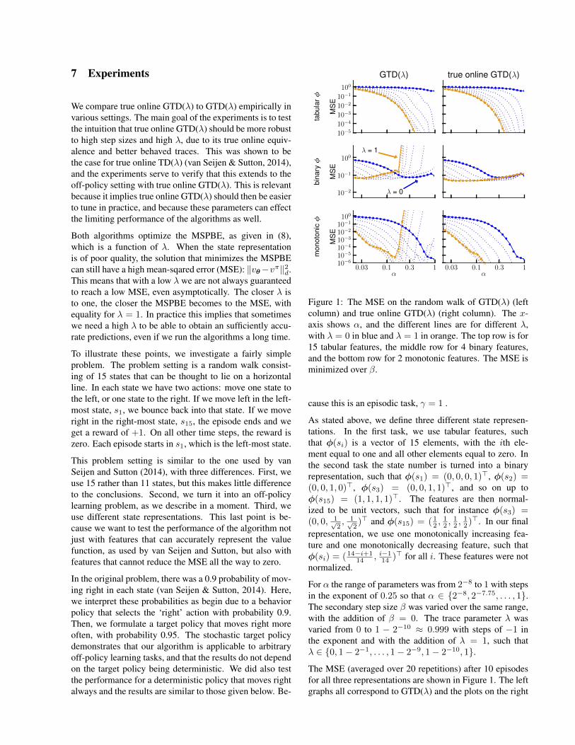
Figure 1: The MSE on the random walk of GTD(λ) (leftcolumn) and true online GTD(λ) (right column). The x-axis shows α, and the different lines are for different λ,with λ = 0 in blue and λ = 1 in orange. The top row is for15 tabular features, the middle row for 4 binary features,and the bottom row for 2 monotonic features. The MSE isminimized over β.

cause this is an episodic task, γ = 1 .

As stated above, we define three different state represen-tations. In the first task, we use tabular features, suchthat φ(si) is a vector of 15 elements, with the ith ele-ment equal to one and all other elements equal to zero. Inthe second task the state number is turned into a binaryrepresentation, such that φ(s1) = (0, 0, 0, 1)>, φ(s2) =(0, 0, 1, 0)>, φ(s3) = (0, 0, 1, 1)>, and so on up toφ(s15) = (1, 1, 1, 1)>. The features are then normal-ized to be unit vectors, such that for instance φ(s3) =(0, 0, 1√

2, 1√

2)> and φ(s15) = ( 1

2 ,12 ,

12 ,

12 )>. In our final

representation, we use one monotonically increasing fea-ture and one monotonically decreasing feature, such thatφ(si) = (14−i+1

14 , i−114 )> for all i. These features were notnormalized.

For α the range of parameters was from 2−8 to 1 with stepsin the exponent of 0.25 so that α ∈ {2−8, 2−7.75, . . . , 1}.The secondary step size β was varied over the same range,with the addition of β = 0. The trace parameter λ wasvaried from 0 to 1 − 2−10 ≈ 0.999 with steps of −1 inthe exponent and with the addition of λ = 1, such thatλ ∈ {0, 1− 2−1, . . . , 1− 2−9, 1− 2−10, 1}.

The MSE (averaged over 20 repetitions) after 10 episodesfor all three representations are shown in Figure 1. The leftgraphs all correspond to GTD(λ) and the plots on the right

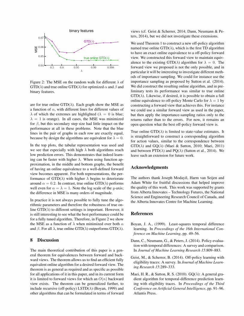
0.5 0.8 0.95 0.99 0.998λ

0.04

0.05

0.06

0.07M

SE

GTD(λ)

true online GTD(λ)

binary features

Figure 2: The MSE on the random walk for different λ ofGTD(λ) and true online GTD(λ) for optimized α and β andbinary features.

are for true online GTD(λ). Each graph show the MSE asa function of α, with different lines for different values ofλ of which the extremes are highlighted (λ = 0 is blue;λ = 1 is orange). In all cases, the MSE was minimizedfor β, but this secondary step size had little impact on theperformance at all in these problems. Note that the bluelines in the pair of graphs in each row are exactly equal,because by design the algorithms are equivalent for λ = 0.

In the top plots, the tabular representation was used andwe see that especially with high λ both algorithms reachlow prediction errors. This demonstrates that indeed learn-ing can be faster with higher λ. When using function ap-proximation, in the middle and bottom graphs, the benefitof having an online equivalence to a well-defined forwardview becomes apparent. For both representations, the per-formance of GTD(λ) with higher λ begins to deterioratearound α = 0.2. In contrast, true online GTD(λ) performswell even for α = λ = 1. Note the log scale of the y-axis;the difference in MSE is many orders of magnitude.

In practice it is not always possible to fully tune the algo-rithmic parameters and therefore the robustness of true on-line GTD(λ) to different settings is important. However, itis still interesting to see what the best performance could befor a fully tuned algorithm. Therefore, in Figure 2 we showthe MSE as a function of λ when minimized over both αand β. For all λ, true online GTD(λ) outperforms GTD(λ).

8 Discussion

The main theoretical contribution of this paper is a gen-eral theorem for equivalences between forward and back-ward views. The theorem allows us to find an efficient fullyequivalent online algorithm for a desired forward view. Thetheorem is as general as required and as specific as possiblefor all applications of it in this paper, and in its current formit is limited to forward views for which an O(n) backwardview exists. The theorem can be generalized further, toinclude recursive (off-policy) LSTD(λ) (Boyan, 1999) andother algorithms that can be formulated in terms of forward

views (cf. Geist & Scherrer, 2014; Dann, Neumann & Pe-ters, 2014), but we did not investigate these extensions.

We used Theorem 1 to construct a new off-policy algorithmnamed true online GTD(λ), which is the first TD algorithmto have an exact online equivalence to a off-policy forwardview. We constructed this forward view to maintain equiv-alence to the existing GTD(λ) algorithm for λ = 0. Theforward view we proposed is not the only possible, and inparticular it will be interesting to investigate different meth-ods of importance sampling. We could for instance use theimportance sampling as proposed by Sutton et al. (2014).We did construct the resulting online algorithm, and in pre-liminary tests its performance was similar to true onlineGTD(λ). Likewise, if desired, it is possible to obtain a fullonline equivalence to off-policy Monte Carlo for λ = 1 byconstructing a forward view that achieves this. For instancewe could use a similar forward view as used in the paper,but then apply the importance-sampling ratios only to thereturns rather than to the errors. For now, it remains anopen question what the best off-policy forward view is.

True online GTD(λ) is limited to state-value estimates. Itis straightforward to construct a corresponding algorithmfor action values, similar to the correspondence betweenGTD(λ) and GQ(λ) (Maei & Sutton, 2010; Maei, 2011)and between PTD(λ) and PQ(λ) (Sutton et al., 2014). Weleave such an extension for future work.

Acknowledgments

The authors thank Joseph Modayil, Harm van Seijen andAdam White for fruitful discussions that helped improvethe quality of this work. This work was supported by grantsfrom Alberta Innovates – Technology Futures, the NationalScience and Engineering Research Council of Canada, andthe Alberta Innovates Centre for Machine Learning.

References

Boyan, J. A., (1999). Least-squares temporal differencelearning. In Proceedings of the 16th International Con-ference on Machine Learning, pp. 49–56.

Dann, C., Neumann, G., & Peters, J. (2014). Policy evalua-tion with temporal differences: A survey and comparison.In Journal of Machine Learning Research 15:809–883.

Geist, M., & Scherrer, B. (2014). Off-policy learning witheligibility traces: A survey. In Journal of Machine Learn-ing Research 15:289–333.

Maei, H. R., & Sutton, R. S. (2010). GQ(λ): A general gra-dient algorithm for temporal-difference prediction learn-ing with eligibility traces. In Proceedings of the ThirdConference on Artificial General Intelligence, pp. 91–96.Atlantis Press.

Maei, H. R. (2011). Gradient Temporal-Difference Learn-ing Algorithms. PhD thesis, University of Alberta.

Precup, D., Sutton, R. S., & Singh, S. (2000). Eligibilitytraces for off-policy policy evaluation. In Proceedings ofthe 17th International Conference on Machine Learning,pp. 759–766. Morgan Kaufmann.

Rubinstein, R. Y. (1981). Simulation and the Monte Carlomethod. New York, Wiley.

Sutton, R. S. (1988). Learning to predict by the methods oftemporal differences. Machine Learning 3:9–44.

Sutton, R. S., Barto, A. G. (1998). Reinforcement Learn-ing: An Introduction. MIT Press.

Sutton, R. S., Mahmood, A. R. , Precup, D., & van Has-selt, H. (2014). A new Q(λ) with interim forward viewand Monte Carlo equivalence. In Proceedings of the 31stInternational Conference on Machine Learning. JMLRW&CP 32(2).

Sutton, R. S., Maei, H. R., Precup, D., Bhatnagar, S., Sil-ver, D., Szepesvari, Cs., & Wiewiora, E. (2009). Fastgradient-descent methods for temporal-difference learn-ing with linear function approximation. In Proceedingsof the 26th Annual International Conference on MachineLearning, pp. 993–1000, ACM.

Sutton, R. S., Modayil, J., Delp, M., Degris, T., Pilarski,P. M., White, A., & Precup, D. (2011). Horde: A scal-able real-time architecture for learning knowledge fromunsupervised sensorimotor interaction. In Proceedings ofthe 10th International Conference on Autonomous Agentsand Multiagent Systems, pp. 761–768.

Sutton, R. S., Szepesvari, Cs., & Maei, H. R. (2008).A convergent O(n) algorithm for off-policy temporal-difference learning with linear function approximation.In Advances in Neural Information Processing Systems21, pp. 1609–1616. MIT Press.

van Seijen, H., & Sutton, R. S. (2014). True online TD(λ).In Proceedings of the 31st International Conference onMachine Learning. JMLR W&CP 32(1):692–700.