
Pkp Tk Pengembangan Kemampuan Berbahasa Melalui Metode Bercakap cakap Pada Anak Kelompok b Tk

FUNDAMENTALS OF HYDROCARBON EXPLORATION AND APPRAISAL
CONTENTSINTRODUCTION 1. THE FIELD LIFE CYCLE 1.1 Exploration Phase1.2 Appraisal Phase1.3 Development Planning1.4 Production Phase
2. EXPLORATION 2.1 Hydrocarbon Accumulations Overview2.2 Exploration Methods and Techniques
3. DRILLING ENGINEERING 4. SAFETY AND THE ENVIRONMENT 5. RESERVOIR DESCRIPTION, 5.1 Reservoir geology5.2 Data Gathering5.3 Data Interpretation

6. VOLUMETRIC ESTIMATION 7. FIELD APPRAISAL 8. RESERVOIR DYNAMIC BEHAVIOUR 9. GAS RESERVOIR 10. FLUID DISPLACEMENT IN THE RESERVOIR 11. RESERVOIR SIMULATION 12. ESTIMATING THE RECOVERY FACTOR 13. ESTIMATING THE PRODUCTION PROFILE 14. ENHANCED OIL RECOVERY 15. WELL DYNAMIC BEHAVIOUR 16. SURFACE FACILITIES 17. PRODUCTION OPERATIONS AND MAINTENANCE 18. PETROLEUM ECONOMICS 19. MANAGING THE PRODUCING FIELD 20. MANAGING DECLINE 21. DECOMMISSIONING REFERENCES
CONTENTS

1. THE FIELD LIFE CYCLE
Keywords: exploration, appraisal, feasibility, development planning, production profile, production, abandonment, project economics, cash flow.
Figure 1: The Field Life Cycle and a Simplified Business Model

Phases of a typical oil (or gas) field life cycle. Modified from the Oil & Gas Journal.

1.1 Exploration Phase
Figure 2: Phasing and expenditure of a typical exploration program

1.2 Appraisal Phase
The purpose of development appraisal is therefore to reduce the uncertainties, in particular those related to the producible volumes contained within the structure.
Consequently, the purpose of appraisal in the context of field development is not to find additional volumes of oil or gas.
.

1.3 Development PlanningBased on the results of the feasibility study, and assuming that at least one option is economically viable, a field development plan can now be formulated and subsequently executed. The plan is a key document used for achieving proper communication, discussion and agreement on the activities required for the development of a new field, or extension to an existing development.The field development plan's prime purpose is to serve as a conceptual project specification for subsurface and surface facilities, and the operational and maintenance philosophy required to support a proposal for the required investments.

1.3 Development Planning
It should give management and shareholders confidence that all aspects of the project have been identified, considered and discussed between the relevant parties:
Objectives of the development Petroleum engineering data Operating and maintenance principles Description of engineering facilities Cost and manpower estimates Project planning Budget proposal

Once the field development plan (FDP) is approved, there follows a sequence of activities prior to the first production from the field:
Field Development Plan (FDP) Detailed design of the facilities Procurement of the materials of construction Fabrication of the facilities Installation of the facilities Commissioning of all plant and equipment
1.3 Development Planning

1.4 Production PhaseThe production phase commences with
the first commercial quantities of hydrocarbons ("first oil") flowing through the wellhead.
This marks the turning point from a cash flow point of view, since from now on cash is generated and can be used to pay back the prior investments, or may be made available for new projects.
The production profile shown in Figure 1 is characterised by three phases:
1. Build up period:During this period newly drilled producers are progressively brought on stream.
2. Plateau period: Initially new wells may still be brought on stream but the older wells start to decline. A constant production rate is maintained. This period is typically 2 to 5 years for an oil field, but longer for a gas field.
3. Decline period: During this final (and usually longest) period all producers will exhibit declining production.
1.4 Production Phase

1.5 DecommissioningThe economic lifetime of a project
normally terminates once its net cash flow turns permanently negative, at which moment the field is decommissioned. Since towards the end of field life the capital spending and asset depreciation are generally negligible, economic decommissioning can be defined as the point at which gross income no longer covers operating costs (and royalties). It is of course still technically possible to continue producing the field, but at a financial loss.
Most companies have at least two ways in which to defer the decommissioning of a field or installation:
reduce the operating costs, or increase hydrocarbon throughput

Figure 3: Using money in The Field Life Cycle
1.5 Decommissioning

2. EXPLORATIONKeywords: plate tectonics, sedimentary basins, source rocks, maturation, migration, reservoir rocks, traps, seismic, gravity survey, magnetic survey, geochemistry, mudlogs, field studies.Exploration activities are aimed at finding new volumes of hydrocarbons, thus replacing the volumes being produced. The success of a company's exploration efforts determines its prospects of remaining in business in the long term.
2.1 Hydrocarbon Accumulations Overview
The first of these is an area in which a suitable sequence of rocks has accumulated over geologic time, the sedimentary basin. Within that sequence there needs to be a high content of organic matter, the source rock. Through elevated temperatures and pressures these rocks must have reached maturation, the condition at which hydrocarbons are expelled from the source rock.
Migration describes the process which has transported the generated hydrocarbons into a porous type of sediment, the reservoir rock. Only if the reservoir is deformed in a favorable shape or if it is laterally grading into an impermeable formation does a trap for the migrating hydrocarbons exist.
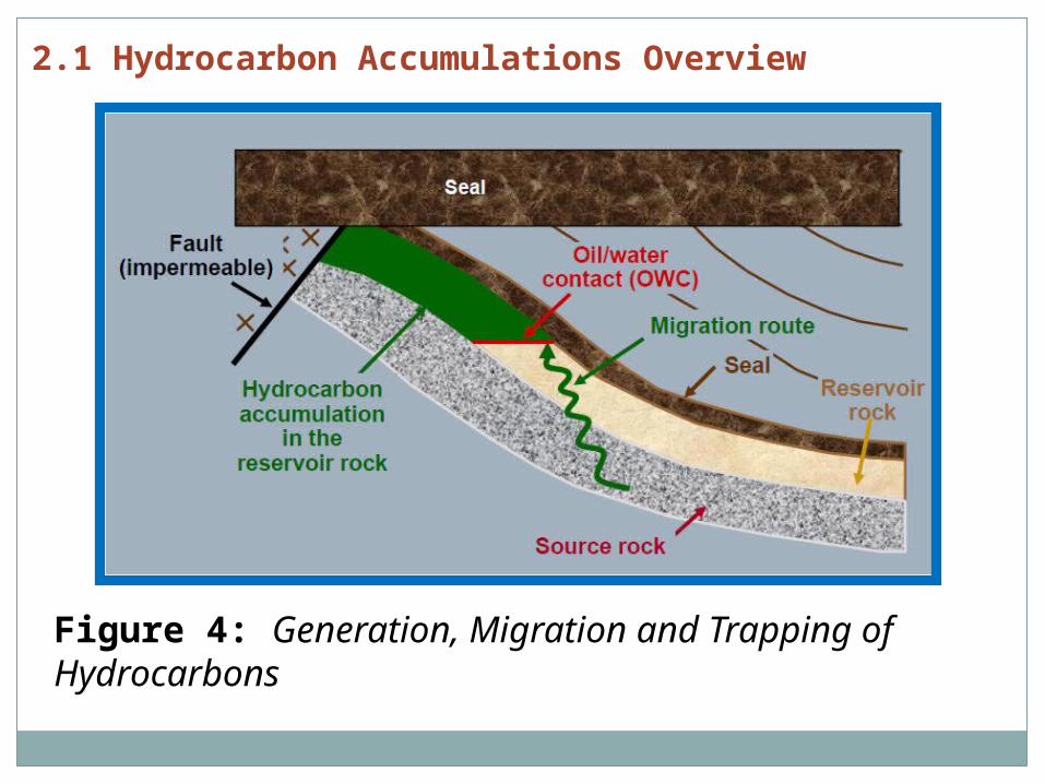
Figure 4: Generation, Migration and Trapping of Hydrocarbons
2.1 Hydrocarbon Accumulations Overview

Figure 5: Global plate configuration
One of the geo-scientific breakthroughs of this century has been the acceptance of the concept of plate tectonics. It is beyond the scope of this book to explore the underlying theories in any detail.
Sedimentary Basins
2.1 Hydrocarbon Accumulations Overview
Sedimentary Basins
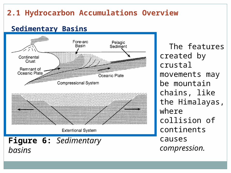
Figure 6: Sedimentary basins
The features created by crustal movements may be mountain chains, like the Himalayas, where collision of continents causes compression.
2.1 Hydrocarbon Accumulations Overview

Source Rocks About 90% of all the organic matter found in sediments is contained in shales. For the deposition of these source rocks several conditions have to be met: organic material must be abundant and a lack of oxygen must prevent the decomposition of the organic remains. Continuous sedimentation over a long period of time causes burial of the organic matter.
2.1 Hydrocarbon Accumulations Overview

Maturation The conversion of sedimentary organic matter into petroleum is termed maturation. The resulting products are largely controlled by the composition of the original matter.
Figure 7: Hydrocarbon migration
2.1 Hydrocarbon Accumulations Overview
MigrationThe maturation of source rocks is followed by the migration of the produced hydrocarbons from the deeper, hotter parts of the basin into suitable structures. During primary migration the very process of kerogen transformation causes micro-fracturing of the impermeable and low porosity source rock which allows hydrocarbons to move into more permeable strata. In the second stage of migration the generated fluids move more freely along bedding planes and faults into a suitable reservoir structure.
2.1 Hydrocarbon Accumulations Overview

Reservoir rock Reservoir rocks are either of clastic or carbonate composition. The former are composed of silicates, usually sandstone, the latter of biogenetically derived detritus, such as coral or shell fragments. For a reservoir to be effective, the pores need to be in communication to allow migration, and also need to allow flow towards the borehole once a well is drilled into the structure. The pore space is referred to as porosity in oil field terms. Permeability measures the ability of a rock to allow fluid flow through its pore system.
2.1 Hydrocarbon Accumulations Overview
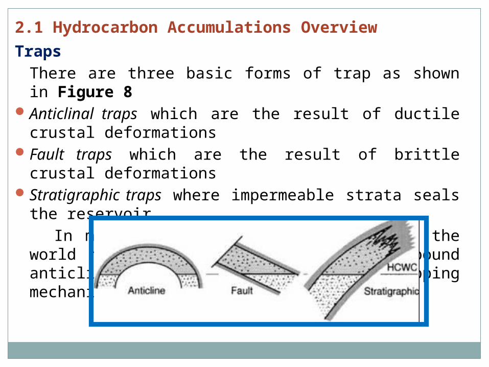
TrapsThere are three basic forms of trap as shown in Figure 8
Anticlinal traps which are the result of ductile crustal deformations
Fault traps which are the result of brittle crustal deformations
Stratigraphic traps where impermeable strata seals the reservoir
In many oil and gas fields throughout the world hydrocarbons are found in fault bound anticlinal structures. This type of trapping mechanism is called a combination trap.
2.1 Hydrocarbon Accumulations Overview
Traps
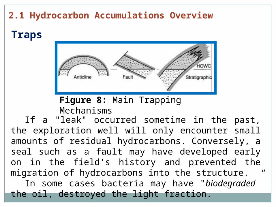
Figure 8: Main Trapping Mechanisms
If a "leak" occurred sometime in the past, the exploration well will only encounter small amounts of residual hydrocarbons. Conversely, a seal such as a fault may have developed early on in the field's history and prevented the migration of hydrocarbons into the structure.
In some cases bacteria may have "biodegraded” the oil, destroyed the light fraction.
2.1 Hydrocarbon Accumulations Overview

PHÂN LOẠI MỎ THEO QUY MÔ
Kích thöôùc moû
Tröõ löôïng khai thaùc (daàu
Tr.T/ khí caân ñoái tyû m3)
Dieän tích moû,
(km2/beà daøy væa saûn phaåm
m)
Khoaûng caùch TB giöõa caùc GK, Km
Moû ñôn giaûn
Moû phöùc taïp
Moû raát phöùc taïp
Cöïc lôùn
>300>500
>1001015
1012 810 58
Raát Lôùn
100300100500
>1001015
4.0(3.54.5)
2.9(2.73.2)
1.8(1.53.0)
Lôùn 30100 25100812
3.0(2.73.3)
2.1(1.82.5)
1.2(0.81.5)
Trung bình
1030 1050510
2.2(1.52.5)
1.5(1.21.7)
1.0(0.81.3)
Nhoû
32538
1.5(1.21.7)
1.5(1.21.7)
1.0(0.51.5)

2.2 Exploration Methods and Techniques
The objective of any exploration venture is to find new volumes of hydrocarbons at a low cost and in a short period of time.The usual sequence of activities once an area has been selected for exploration starts with the definition of a basin.
The mapping of gravity anomalies and magnetic anomalies will be the first two methods applied. In many cases today this data will be available in the public domain or can be bought as a "non exclusive" survey.
Next, a coarse two- dimensional (2D) seismic grid, covering a wide area, will be acquired in order to define leads, areas which show for instance a structure which potentially could contain an accumulation.

Gravity SurveysThe gravity method measures small variations of the earth's gravity field caused by density variations in geological structures. The sensing element is a sophisticated form of spring balance. Variations in the earth's gravity field cause changes in the length of the spring, which are measured
2.2 Exploration Methods and Techniques
Figure 9: Principle of gravity surveys

Magnetic SurveysThe magnetic method detects changes in the earth's magnetic field caused by variations in the magnetic properties of rocks. In particular basement and igneous rocks are relatively highly magnetic and if close to the surface give rise to short wavelength, high amplitude anomalies in the earth's magnetic field (Fig. 10). The method is airborne (plane or satellite) which permits rapid surveying and mapping with good areal coverage. Like the gravity technique this survey is often employed at the beginning of an exploration venture.
2.2 Exploration Methods and Techniques

Magnetic Surveys
Figure 10: Principle of magnetic surveys
2.2 Exploration Methods and Techniques
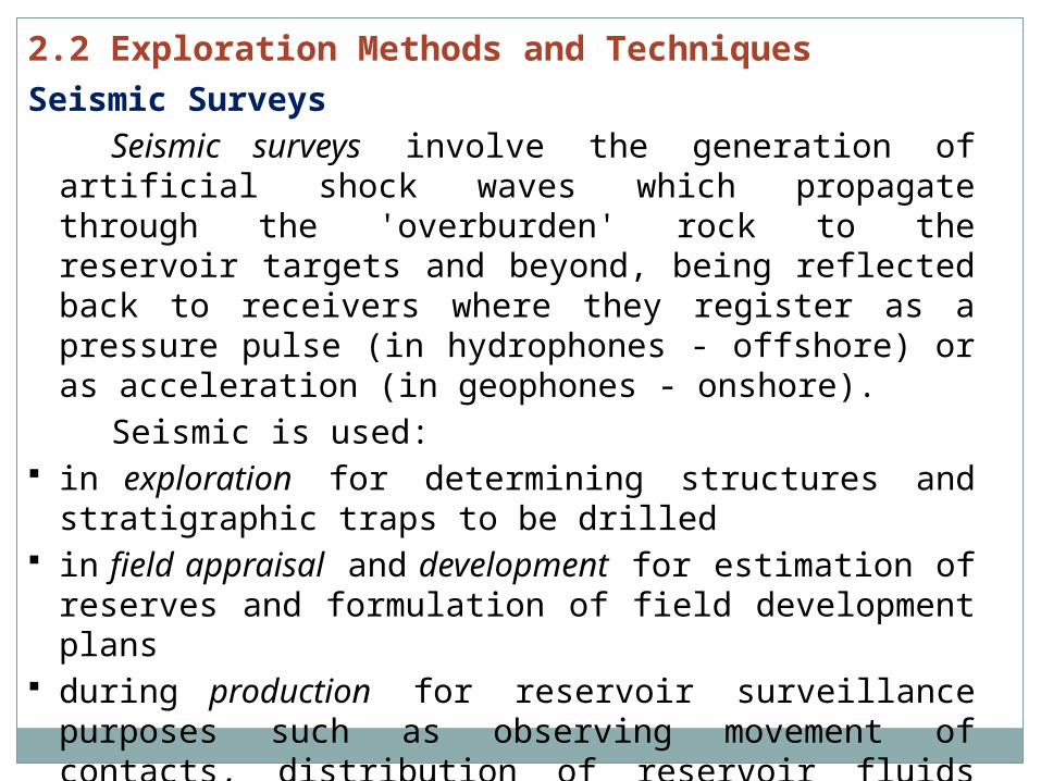
Seismic SurveysSeismic surveys involve the generation of
artificial shock waves which propagate through the 'overburden' rock to the reservoir targets and beyond, being reflected back to receivers where they register as a pressure pulse (in hydrophones - offshore) or as acceleration (in geophones - onshore).
Seismic is used: in exploration for determining structures and stratigraphic traps to be drilled
in field appraisal and development for estimation of reserves and formulation of field development plans
during production for reservoir surveillance purposes such as observing movement of contacts, distribution of reservoir fluids and changes in pressure
2.2 Exploration Methods and Techniques

Seismic Surveys There are actually different wave types that propagate in solid rock, but the first arrival (i.e. fastest ray path) is normally the compressional or P wave. The two attributes that are measured are
reflection time (related to depth of the reflector, and velocity in the overburden), and
amplitude, related to rock properties in the reflecting interval, as well as to various extraneous influences that have to be removed in processing.
2.2 Exploration Methods and Techniques
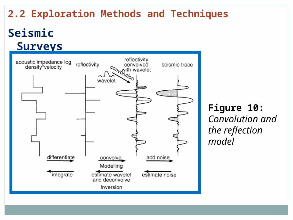
Seismic Surveys
Figure 10: Convolution and the reflection model
2.2 Exploration Methods and Techniques

Seismic Surveys
Figure 11: acquisition system
2.2 Exploration Methods and Techniques

Seismic SurveysInterpretation involvesPicking intervals or horizons of interest deriving the structure of the field or potential trap (both the stratigraphic detail and the faulting) getting some insight into the reservoir quality variations, such as porosity, of interest to the petroleum engineer or geologist.
2.2 Exploration Methods and Techniques

GeochemistryGeochemistry is employed for the following reasons:
To detect surface anomalies caused by hydrocarbon accumulations: often very small amounts of petroleum compounds have leaked into the overlying strata and to the surface. On land, these compounds, mostly gases, may be detectable in soil samples.
To assess potential yield and maturity of source rocks and classify those according to their "vitrinite reflectance".
2.2 Exploration Methods and Techniques

Geochemistry
Figure 12: Analysis of crude oil components
2.2 Exploration Methods and Techniques

Field studiesDetailed investigation of a suitable outcrop can often be used as a predictive tool to model:
presence, maturity and distribution of source rock porosity and permeability of a reservoir detailed reservoir framework, including flow units, barriers and baffles to fluid flow
frequency, orientation and geological history of fractures and sub-seismic faults
lateral continuity of sands and shales quantitative description of all of the above for numerical reservoir simulations
2.2 Exploration Methods and Techniques

Mudlogging The technique of mudlogging is covered in this section because it is one of the first direct evaluation methods available during the drilling of an exploration well. As such, the mudlog remains an important and often under-used source of original information.
This first information about the reservoir is recorded, as a function of depth, in the form of several columns.
2.2 Exploration Methods and Techniques
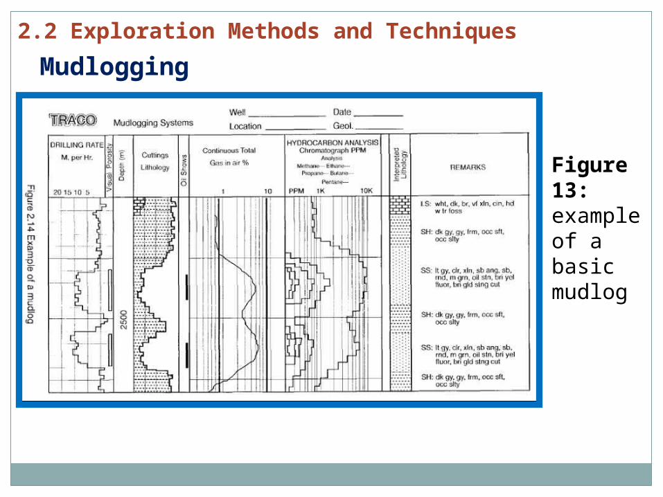
Mudlogging
Figure 13: example of a basic mudlog
2.2 Exploration Methods and Techniques

In summary, exploration activities require the integration of different techniques and disciplines. Clear definition of survey objectives is needed. When planning and executing an exploration campaign the duration of data acquisition and interpretation has to be taken into account.
Figure 14: Summary of exploration objectives and menthods
2.2 Exploration Methods and Techniques

3. DRILLING ENGINEERINGKeywords: well objectives, well planning, rig selection, rotary drilling, site preparation, shallow gas, directional drilling, drilling fluids, rig types, drilling problems, extended reach drilling, slimhole drilling, horizontal wells, coiled tubing drilling, contracts, drilling costs
3.1 Well PlanningCareful planning of drilling activities will
avoid unnecessary expenditure or risks. The planning process is vital for achieving the objectives of a well. Usually, wells are drilled with one, or a combination, of the following objectives:
to gather information to produce hydrocarbons « to inject gas or water
to relieve a blowout

3.2 Rig Types and Rig SelectionThe type of rig which will be selected depends upon a number of parameters, in particular:
cost and availabilitywater depth of location (offshore)mobility / transportability (onshore)depth of target zone and expected formation pressures
prevailing weather conditions in the area of operation
quality of the drilling crew
3. DRILLING ENGINEERING

3.2 Rig Types and Rig Selection
Figure 15: Offshore rig type
3. DRILLING ENGINEERING
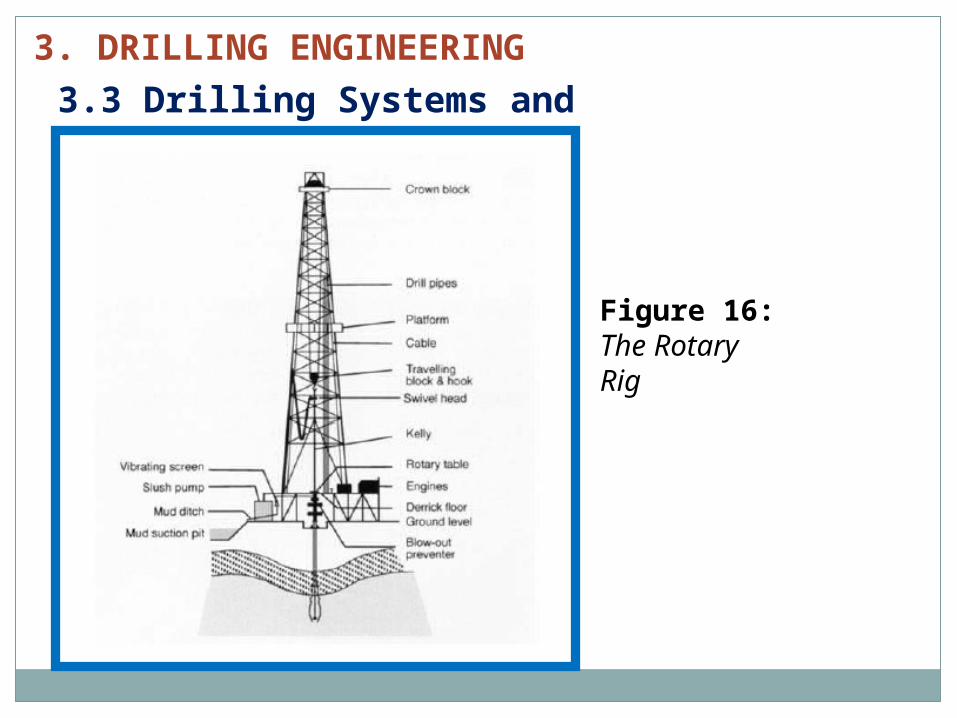
3.3 Drilling Systems and Equipment
Figure 16: The Rotary Rig
3. DRILLING ENGINEERING

4. RESERVOIR DESCRIPTION
The success of oil and gas field development is largely determined by the reservoir; its size, complexity, productivity, and the type and quantity of fluids it contains. To optimise a development plan, the characteristics of the reservoir must be well defined. The section is divided into four parts:
Reservoir geologyHydrocarbon fluidsData gatheringData interpretation
4.1 Reservoir geology
The objective of reservoir geology is the description and quantification of geologically controlled reservoir parameters and the prediction of their lateral variation. Three parameters broadly define the reservoir geology of a field:
depositional environmentstructurediagenesis

4.1.1 Depositional EnvironmentThe two main categories are siliciclastic
rocks, usually referred to as 'clastics' or 'sandstones', and carbonate rocks.
Before looking at the significance of depositional environments for the production process let us investigate some of the main characteristics of both categories.
ClasticsThe deposition of a clastic rock is preceded
by the weathering and transport of material.Weathering results in the breaking up of
rock into smaller components which then can be transported by agents such as water (rivers, sea currents), wind (deserts) and ice (glaciers).
Transport energy determines the size, shape and degree of sorting of sediment grains. Sorting is an important parameter controlling properties such as porosity.

4.1.1 Depositional EnvironmentClastics
The deposition of a clastic rock is preceded by the weathering and transport of material.
Mechanical weathering will be induced if a rock is exposed to severe temperature changes or freezing of water in pores and cracks (e.g. in some desert environments).
The action of plant roots forcing their way into bedrock is another example of mechanical weathering.
Substances (e.g. acid waters) contained in surface waters can cause chemical weathering. During this process minerals are dissolved and the less stable ones, like feldspars are leached.
Chemical weathering is particularly severe in tropical climates.
Impact of sorting on reservoir quality.Quartz (Si02) is one of the most stable minerals and is therefore the main constituent of sandstones which have undergone the most severe weathering and transportation over considerable distance. These sediments are called 'mature' and provide 'clean' high quality reservoir sands. In theory, porosity is not affected by the size of the grains but is purely a percentage of the bulk rock volume. In nature however, sands with large well sorted components may have higher porosities than the equivalent sand comprising small components. This is simply the result of the higher transport energy required to move large components, hence a low probability of fine (light) particles such as clay being deposited.

Figure 17: Types of clay distribution

Carbonate rocks Weathering and transportation is followed by the sedimentation of material. The depositional environment can be defined as an area with a typical set of physical, chemical and biological processes which result in a specific type of rock. The characteristics of the resulting sediment package are dependent on the intensity and duration of these processes. The physical, chemical, biological and geomorphic variables show considerable differences between and within particular environments. As a result, we have to expect very different behaviour of such reservoirs during hydrocarbon production. Depositional processes control porosity, permeability, net to gross ratio, extent and lateral variability of reservoir properties. Hence the production profile and ultimate recovery of individual wells and accumulations are heavily influenced by the environment of deposition.

• There exists an important relationship between the depositional environment, reservoir distribution and the production characteristics of a field (Figure 18-1, 18-2)

Depositional Environment
Reservoir Distribution
Production Characteristic
Deltaic (distributary
channel)
Isolated or stacked channels usually with tine grained sands. May or may not be in communication
Good producers: permeabilities of 500÷5000mD. Insufficient communication between channels may require infill wells in late stage of development
Shallow marine/coastal
(clastic)
Sand bars, tidal channels. Generally coarsening High subsidence rate results in 'stacked' reservoirs. Reservoir distribution dependent on wave and tide action
Prolific producers as a result of 'clean' and continuous sand bodies. Shale layers may cause vertical barriers to fluid flax
Figure 18-1

Depositional Environment
Reservoir Distribution
Production Characteristic
Shallow water carbonate (reefs & carbonate muds)
Reservoir quality governed by diagenetic processes and structural history (fracturing)
Prolific production from karstified carbonates. High and early water production possible. 'Dual porosity' systems in fractured carbonates. Dolomites may produce H2S
Shelf (elastics) Sheet-like sandbodies resulting from storms or transgression. Usually thin but very continuous sands, well sorted and coarse between marine clays
Very high productivity but high quality sands may act as 'thief zones' during water or gas injection. Action of sediment burrowing organisms may impact on reservoir quality
Figure 18-2

4.1.2 Reservoir Structures
Like any other material, rocks may react to stress with an elastic, ductile or brittle response, as described in the stress-strain diagram in Figure 19.
Figure 19: The stress - strain diagram for a reservoir rock

Four mechanisms have been suggested to explain how faults provide seals. The most frequent case is that of clay smear and juxtaposition (Figure. 20)
Clay smear: soft clay, often of marine origin, is smeared into the fault plane during movement and provides an effective seal.
Juxtaposition: faulting has resulted in an impermeable rock 'juxtaposed' against a reservoir rock.
Other, less frequent fault seals are created by:
Diagenetic Healing: late precipitation of minerals on or near the fault plane has created a sealing surface (see "diagenesis" for more detail).
Cataclasis: the fault movement has destroyed the rock matrix close to the fault plane. Individual quartz grains have been 'ground up' creating a seal comprising of "rock flour".

Figure 20: Fault seal as a result of clay smear and juxtaposition

Folds are features related to compressional, ductile deformation (Fig. 21). They form some of the largest reservoir structures known. A fold pair consists of anticline and syncline.
Figure 21: Fold terminology

4.3 Data GatheringIntroduction and commercial application: Data gathering is an activity which provides the geologist and engineer with the information required to estimate the volume of the reservoir, its fluid content, productivity, and potential for development. Data gathering is not only carried out at the appraisal and development planning stage of the field life cycle, but continues throughout the field life. This section will focus on the data gathered for field development planning; data gathering for managing the field during the production period is discussed in Section 14.0.
The timely acquisition of static and dynamic reservoir data is critical for the optimisation of development options and production operations. Reservoir data enables the description and quantification of fluid and rock properties. The amount and accuracy of the data available will determine the range of uncertainty associated with estimates made by the subsurface engineer.

4.3 Data Gathering 4.3.1 Classification of methodsThe basic data gathering methods are direct
methods which allow visual inspection or at least direct measurement of properties, and indirect methods whereby we infer reservoir parameters from a number of measurements taken in a borehole. The main techniques available within these categories are summarised in the following table:Direct Indirect
Coring WirelineSidewall sampling Logging while
drilling (LWD)Mudlogging SeismicFormation pressure samplingFluid sampling

To gain an understanding of the composition of the reservoir rock, inter-reservoir seals and the reservoir pore system it is desirable to obtain an undisturbed and continuous reservoir core sample. Cores are also used to establish physical rock properties by direct measurements in a laboratory. They allow description of the depositional environment, sedimentary features and the diagenetic history of the sequence.
In the pre-development stage, core samples can be used to test the compatibility of injection fluids with the formation, to predict borehole stability under various drilling conditions and to establish the probability of formation failure and sand production.
Coring is performed in between drilfing operations. Once the formation for which a core is required has been identified on the mud log, the drilling assembly is pulled out of hole. For coring operations a special assembly is run on drill pipe (Fig. 22) comprising a core bit and a core barrel.
4.3 Data Gathering 4.3.2 Coring and core analysis
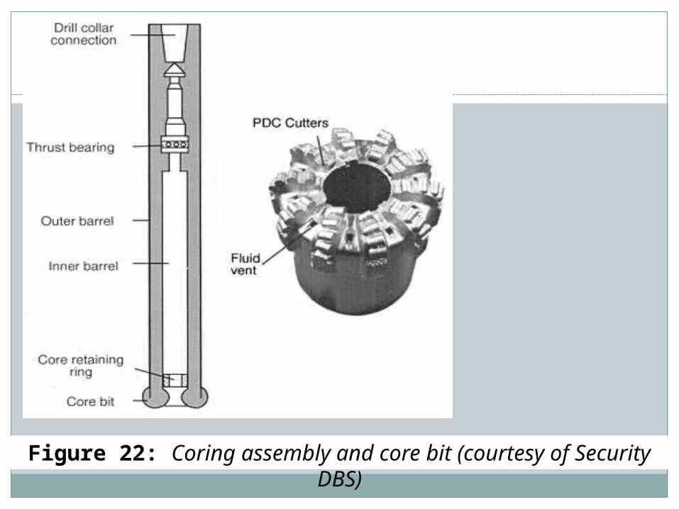
Figure 22: Coring assembly and core bit (courtesy of Security DBS)

The sidewall sampling tool (SWS) can be used to obtain small plugs (2 cm diameter, 5 cm length, often less) directly from the borehole wall. The tool is run on wireline after the hole has been drilled. Some 20 to 30 individual bullets are fired from each gun (Fig. 23) at different depths. The hollow bullet will penetrate the formation and a rock sample will be trapped inside the steel cylinder. By pulling the tool upwards, wires connected to the gun pull the bullet and sample from the borehole wall.
SWS are useful to obtain direct indications of hydrocarbons (under UV light) and to differentiate between oil and gas. The technique is applied extensively to sample microfossils and pollen for stratigraphic analysis (age dating, correlation, depositional environment). Qualitative inspection of porosity is possible, but very often the sampling process results in a severe crushing of the sample thus obscuring the true porosity and permeability.
4.3 Data Gathering4.3.3 Sidewall sampling

Figure 23: Sidewall coring tool

Wireline logs represent a major source of data for geoscientists and engineers investigating subsurface rock formations. Logging tools are used to look for reservoir quality rock, hydrocarbons and source rocks in exploration wells, support volumetric estimates and geological modelling during field appraisal and development, and provide a means of monitoring the distribution of remaining hydrocarbons during the production life time.
A large investment is made by oil and gas companies in acquiring open hole log data. Logging activities can represent up to 10% of the total well cost. It is important therefore to ensure that the cost of acquisition can be justified by the value of information generated and that thereafter the information is effectively managed.
4.3 Data Gathering4.3.4 Wireline logging

Figure 24: Principle of wireline logging Figure 25: MDT tool
configuration for permeability measurement
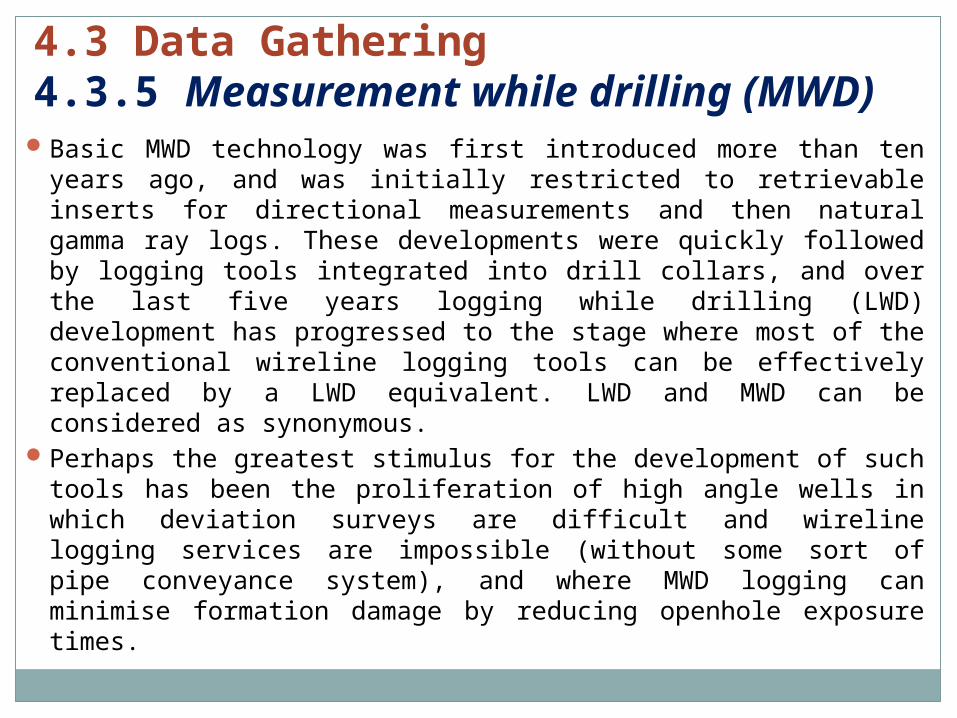
Basic MWD technology was first introduced more than ten years ago, and was initially restricted to retrievable inserts for directional measurements and then natural gamma ray logs. These developments were quickly followed by logging tools integrated into drill collars, and over the last five years logging while drilling (LWD) development has progressed to the stage where most of the conventional wireline logging tools can be effectively replaced by a LWD equivalent. LWD and MWD can be considered as synonymous.
Perhaps the greatest stimulus for the development of such tools has been the proliferation of high angle wells in which deviation surveys are difficult and wireline logging services are impossible (without some sort of pipe conveyance system), and where MWD logging can minimise formation damage by reducing openhole exposure times.
4.3 Data Gathering4.3.5 Measurement while drilling (MWD)

Whilst providing deviation and logging options in high angle wells is a considerable benefit, the greatest advantage offered by MWD technology, in either conventional or high angle wells, is the acquisition of real time data at surface. Most of the MWD applications which are now considered standard exploit this feature in some way, and include:
real time correlation for picking coring and casing points
real time overpressure detection in exploration wellsreal time logging to minimise 'out of target' sections (geosteering)
real time formation evaluation to facilitate 'stop drilling' decisions
4.3 Data Gathering4.3.5 Measurement while drilling (MWD)

Introduction and Commercial Application: This section introduces the main methods used to convert raw well data into useful information; information with which to characterise the reservoir. A huge volume of data is generated by drilling and logging a typical well. Collecting and storing data requires substantial investment but unless it is processed and presented appropriately much of the potential value is not realised. Describing a reservoir can be a simple task if it has been laid down as a thick blanket of sand, but becomes increasingly complex where hydrocarbons are found in, for example, ancient estuarine or reef deposits. In all cases however there are two main issues which need to be resolved; firstly how much oil does the reservoir contain (the hydrocarbons initially in place - HCIIP), and secondly how much can be recovered (the ultimate recovery - UR). There are a number of ways to determine these volumes (which will be explained in Section 7.0) but the basic physical parameters for describing the reservoir remain the same:
net reservoir thickness hydrocarbon saturation Porosity Permeability
4.4 Data Interpretation

Well correlation is used to establish and visualise the lateral extent and the variations of reservoir parameters. In carrying out a correlation we subdivide the objective sequence into lithologic units and follow those units or their generic equivalent laterally through the area of interest. As we have seen earlier the reservoir parameters such as net to gross ratio (N/G), porosity, permeability etc. are to a large extent controlled by the reservoir geology, in particular the depositional environment. Thus, by correlation we can establish lateral and vertical trends of those parameters throughout the structure. This will enable us to calculate hydrocarbon volumes in different parts of a field, predict production rates and optimise the location for appraisal and development wells.
Usually well logs are only one type of data used to establish a correlation. Any meaningful interpretation will need to be supported by palaeontological data (micro fossils) and palynological data (pollen of plants). The logs most frequently used for correlation are : GR, density logs, sonic log, dipmeter, formation imaging tools. On a detailed scale, these curves should always be calibrated with core data as described below.
4.4 Data Interpretation 4.4.1 Well correlation

On a larger scale, for example in a regional context, seismic stratigraphy will help to establish a reliable correlation. It is employed in combination with the concept of sequence stratigraphy. This technique, initially introduced some 15 years ago by Exxon Research, and since then considerably refined, postulates that global ('eustatid) sea level changes create unconformities which can be used to subdivide the stratigraphic record. These unconformities are modified and affected by more local ('relative') changes in sea level as a result of local tectonic movements, climate and the resulting impact on sediment supply. The most significant stratigraphic discontinuities used in a sequence stratigraphic approach are regressive surfaces of erosion, caused by a lowering of sea level
transgressive surfaces of erosion, caused by an increase in sea level
maximum flooding surfaces at times of 'highest' sea level
4.4 Data Interpretation 4.4.1 Well correlation
Sequence stratigraphy integrates information gleaned from seismic, cores, well logs and often outcrops. In many cases it has increased the understanding of reservoir geometry and heterogeneity and improved the correlation of individual drainage units. Sequence stratigraphy has also proved a powerful tool to predict presence and regional distribution of reservoirs. For instance, shallow marine regressive surfaces may indicate the presence of turbidites in a nearby, deeper marine area.
4.4 Data Interpretation 4.4.1 Well correlation

In preparation for a field wide 'quick look' correlation, all well logs need to be corrected for borehole inclination. This is done routinely with software which uses the measured depth below the derrick floor ('alonghole depth' below derrick floor AHBDFor 'measured depth', MD ) and the acquired directional surveys to calculate the true vertical depth subsea (TVSS). This is the vertical distance of a point below a common reference level, for instance chart datum (CD) or mean sea level (MSL). Figure 26 shows the relationship between the different depth measurements.
4.4 Data Interpretation 4.4.1 Well correlation

To start the correlation process we take the set of logs and select a datum plane. This is a marker which can be traced through all data points (three wells in the example of Figure 27). A good datum plane would be a continuous shale because we can assume that it represents a 'flooding surface' present over a wide area. Since shales are low energy deposits we may also assume that they have been deposited mostly horizontally, blanketing the underlying sediments thus 'creating' a true datum plane.
4.4 Data Interpretation 4.4.1 Well correlation

Figure 26: Depth measurements used
Next, we align all logs at the datum plane which now becomes a straight horizontal line. Note that by doing so we ignore all structural movements to which the sequence has been exposed.
We can now correlate all 'events' below or above the datum plane by comparing the log response. In many instances
4.4 Data Interpretation 4.4.1 Well correlation

Figure 27: Datum plane correlation

Introduction and Commercial Application: The objective of performing appraisal activities on discovered accumulations is to reduce the uncertainty in the description of the hydrocarbon reservoir, and to provide information with which to make a decision on the next action. The next action may be, for example, to undertake more appraisal, to commence development, to stop activities, or to sell the prospect. In any case, the appraisal activity should lead to a decision which yields a greater value than the outcome of a decision made in the absence of the information from the appraisal. The improvement in the value of the action, given the appraisal information, should be greater than the cost of the appraisal activities, otherwise the appraisal effort is not worthwhile.
5.0 FIELD APPRAISAL
• Appraisal activity should be prioritised in terms of the amount of reduction of uncertainty it provides, and its impact on the value derived from the subsequent action.
• The objective of appraisal activity is not necessarily to prove more hydrocarbons. For example, appraisal activity which determines that a discovery is non-commercial should be considered as worthwhile, since it saves a financial loss which would have been incurred if development had taken place without appraisal.
• This section will consider the role of appraisal in the field life cycle, the main sources of uncertainty in the description of the reservoir, and the appraisal techniques used to reduce this uncertainty. The value of the appraisal activity will be compared with its cost to determine whether such activity is justified.
5.0 FIELD APPRAISAL

• Appraisal activity, if performed, is the step in the field life cycle between the discovery of a hydrocarbon accumulation and its development. The role of appraisal is to provide cost-effective information with which the subsequent decision can be made. Cost effective means that the value of the decision with the appraisal information is greater than the value of the decision without the information. If the appraisal activity does not add more value than its cost, then it is not worth doing. This can be represented by a simple flow diagram, in which the cost of appraisal is $A, the profit (net present value) of the development with the appraisal information is $(D2-A), and the profit of the development without the appraisal information is $D1.
5.0 FIELD APPRAISAL 5.1 The role of appraisal in the field life cycle

Figure 28: Net present value with and without appraisal
The appraisal activity is only worthwhile if the value of the outcome with the appraisal information is greater than the value of the outcome without the information
i.e. D2 -A > D1or A < D2-D1
In other words, the cost of the appraisal must be less than the improvement in the value of the development which it provides. It is often necessary to assume outcomes of the appraisal in order to estimate the value of the development with these outcomes.
5.0 FIELD APPRAISAL 5.1 The role of appraisal in the field life cycle

Field appraisal is most commonly targeted at reducing the range of uncertainty in the volumes of hydrocarbons in place, where the hydrocarbons are, and the prediction of the performance of the reservoir during production.
The parameters which are included in the estimation of STOIIP, GIIP and ultimate recovery, and the controlling factors are shown in the following table.
5.0 FIELD APPRAISAL5.2 Identifying and quantifying sources of uncertainty
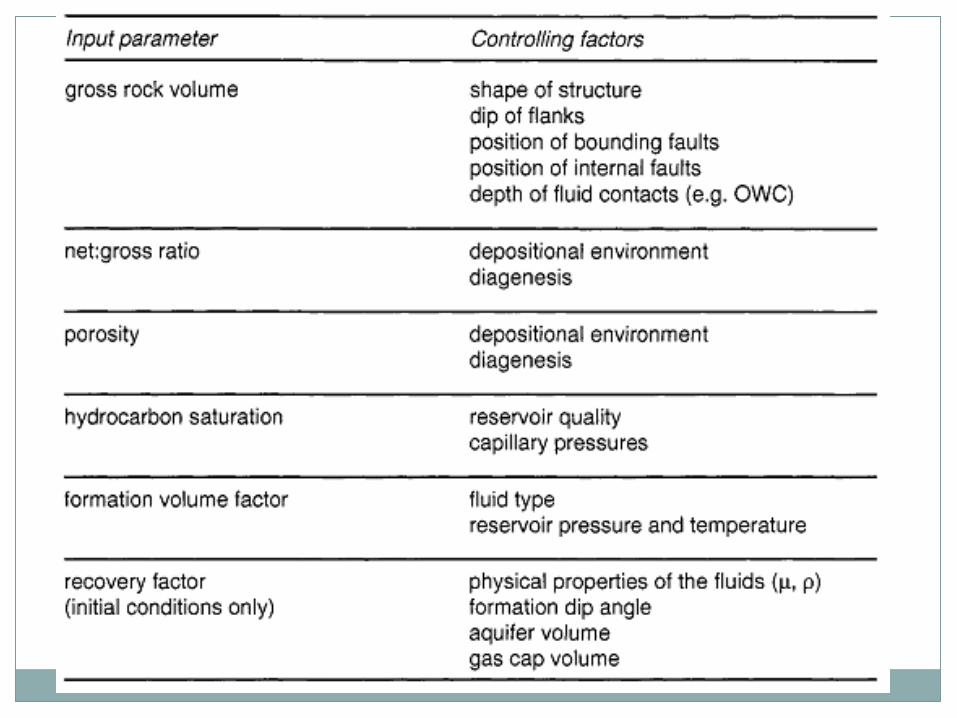

It should be noted that the recovery factor for a reservoir is highly dependent upon the development plan, and that initial conditions alone cannot be used to determine this parameter.
In determining an estimate of reserves for an accumulation, all of the above parameters will be used. When constructing an expectation curve for STOMP, GIIP, or ultimate recovery, a range of values for each input parameter should be used, as discussed in Section 6.2. In determining an appraisal plan, it is necessary to determine which of the parameters contributes most to the uncertainty in STOIIP, GIIP, or UR.
Take an example of estimating gross rock volume, based on seismic data and the results of two wells in a structure (Fig. 29). The following cross-section has been generated, and a base case GRV has been calculated.
5.0 FIELD APPRAISAL5.2 Identifying and quantifying sources of uncertainty

The general list of factors influencing the uncertainty in the gross rock volume included the shape of structure, dip of flanks, position of bounding faults, position of internal faults, and depth of fluid contacts (in this case the OWC). In the above example, the OWC is penetrated by two wells, and the dip of the structure can be determined from the measurements made in the wells which in turn will allow calibration of the 3D seismic.
5.0 FIELD APPRAISAL5.2 Identifying and quantifying sources of uncertainty
The most significant sources of uncertainty in GRV are probably the position and dip of the bounding fault, and the extent of the field in the plane perpendicular to this section. By looking at the quality of the seismic data, an estimate may be made of the uncertainty in the position of the fault, and any indications of internal faulting which may affect the volumetrics. The determination of geological uncertainties requires knowledge of the environment of deposition, diagenesis, and the structural pattern of the field. The quantification often starts with a subjective estimate based on regional knowledge of the geology. In cases where little data is available, "guesstimates" may need to be supplemented with data or reservoir trends observed in neighbouring fields.
5.0 FIELD APPRAISAL5.2 Identifying and quantifying sources of uncertainty

Figure 29: Partially appraised structure

The example illustrates some important steps in identifying the uncertainties and then beginning to quantify them:
consider the factors which influence the parameter being assessed
rank the factors in order of the degree of influence
consider the uncertainties in the data used to describe the factor
The same procedure may be used to rank the parameters themselves (GRV, N/G, <j>, Sh, B0, recovery factor), to indicate which has the greatest influence on the HCIIP or ultimate recovery (UR).
The ranking process is an important part of deciding an appraisal programme, since the activities should aim to reduce the uncertainty in those parameters which have the most impact on the range of uncertainty in HCIIP or UR.
5.0 FIELD APPRAISAL5.2 Identifying and quantifying sources of uncertainty

The main tools used for appraisal are those which have already been discussed for exploration, namely drilling wells and shooting 2-D or 3-D seismic surveys.
Appraisal activity may also include re-processing an existing old seismic survey (again, 2-D or 3-D) using new processing techniques to improve the definition. It is not necessary to re-process the whole survey data set; a sample may be re-processed to determine whether the improvement in definition is worthwhile. In the majority of cases where only 2D seismic is available, time and money will be better spent on shooting a new 3D seismic survey.
5.0 FIELD APPRAISAL5.3 Appraisal tools

Seismic surveys are traditionally an exploration and appraisal tool. However, 3-D seismic is now being used more widely as a development tool, i.e. applied for assisting in selecting well locations, and even in identifying remaining oil in a mature field. This was discussed in Section 2.0. Seismic data acquired at the appraisal stage of the field life is therefore likely to find further use during the development period.
Appraisal activity should be based upon the information required.
The first step is therefore to determine what uncertainties appraisal is trying to reduce, and then what information is required to tie down those uncertainties. For example, if fluid contacts are a major source of uncertainty, drilling wells to penetrate the contacts is an appropriate tool; seismic data or well testing may not be.
5.0 FIELD APPRAISAL5.3 Appraisal tools

Other examples of appraisal tools are:an interference test between two wells to determine pressure communication across a faulta well drilled in the flank of a field to improve the control of the dips seen on seismica well drilled with a long enough horizontal section to emerge from the flanks of the reservoir, and determine the extent of the reservoir in the flanks (horizontal wells may provide significantly more appraisal information about reservoir continuity than vertical wells)
5.0 FIELD APPRAISAL5.3 Appraisal tools
Other examples of appraisal tools are:a production test on a well to determine the productivity from future development wells
coring and production testing of the water leg in a field to predict aquifer behaviour during production, or to test for injectivity in the water leg
deepening a well to investigate possible underlying reservoirs
coring a well to determine diagenetic effects
5.0 FIELD APPRAISAL5.3 Appraisal tools

The most informative method of expressing uncertainty in HCIIP or ultimate recovery (UR) is by use of the expectation curve, as introduced in Section 6.2. The high (H) medium (M) and low (L) values can be read from the expectation curve. A mathematical representation of the uncertainty in a parameter (e.g. STOIIP) can be defined as :
% uncertainty = ((H - L)/2M)*100%The stated objective of appraisal activity is to reduce uncertainty. The impact of appraisal on uncertainty can be shown on an expectation curve, if an outcome is assumed from the appraisal. The following illustrates this process.
Suppose that four wells have been drilled in a field, and the geologist has identified three possible top sands maps based on the data available. These maps, along with the ranges of data for the other input parameters (N/G, S0, <J>, B0) have been used to generate an expectation curve for STOIIP.
5.0 FIELD APPRAISAL5.4 Expressing reduction of uncertainty
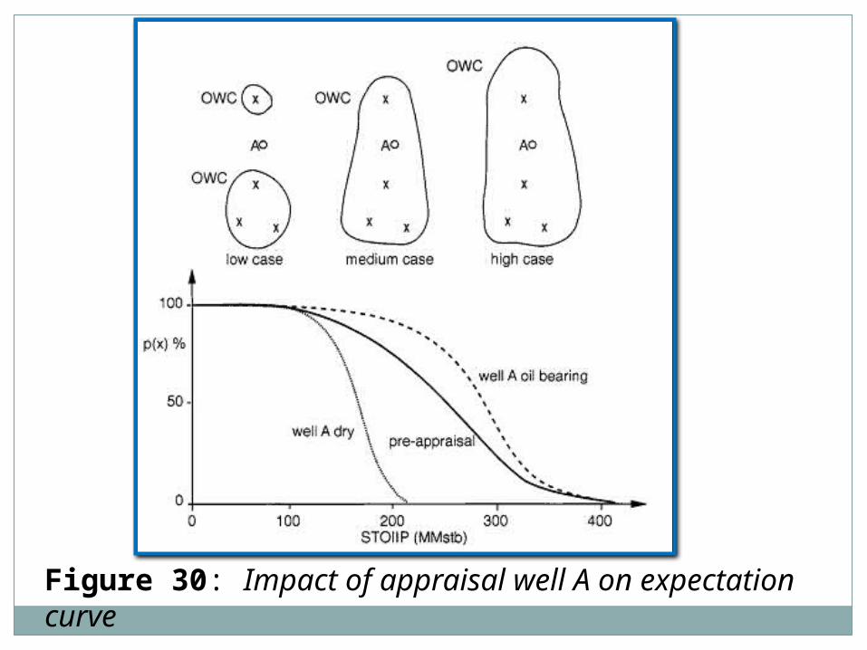
Figure 30: Impact of appraisal well A on expectation curve

If well A is oil bearing, then the low case must increase, though the high case may not be affected. If well A is water bearing (dry), then the medium and high cases must reduce, though the low case may remain the same. For both outcomes, the post-appraisal expectation curve becomes steeper, and the range of uncertainty is reduced.
Note that it is not the objective of the appraisal well to find more oil, but to reduce the range of uncertainty in the estimate of STOMP. Well A being dry does not imply that it is an unsuccessful appraisal well.
The choice of the location for well A should be made on the basis of the position which reduces the range of uncertainty by the most. It may be for example, that a location to the north of the existing wells would actually be more effective in reducing uncertainty. Testing the appraisal well proposal using this method will help to identify where the major source of uncertainty lies.
5.0 FIELD APPRAISAL5.4 Expressing reduction of uncertainty

• As discussed at the beginning of this section, the value of information from appraisal is the difference between the outcome of the decision with the information and the outcome of the decision without the information.
• The determination of the value of the information is assisted by the use of decision trees. Consider the following decision tree as a method of justifying how much should be spent on appraisal. Suppose the range of uncertainty in STOMP prior to appraisal is (20, 48, 100 MMstb; L,M,H values). One can perform appraisal which will determine which of the three cases is actually true, and then tailor a development plan to the STOMP, or one can go ahead with a development in the absence of the appraisal information, only finding out which of the three STOIIPs exist after committing to the development.
• There are two types of nodes in the decision tree: decision nodes (rectangular) and chance nodes (circular). Decision nodes branch into a set of possible actions, while chance nodes branch into all possible results or situations.
5.0 FIELD APPRAISAL5.5 Cost-benefit calculations for appraisal

• The decision tree can be considered as a road map which indicates the chronological order in which a series of actions will be performed, and shows several possible courses, only one of which will actually be followed.
• The tree is drawn by starting with the first decision to be taken, asking which actions are possible, and then considering all possible results from these actions, followed by considering future actions to be taken when these results are known, and so on. The tree is constructed in chronological order, from left to right.
• Then the values of the leaves are placed on the diagram, starting in the far most future; the right hand side. The values represent the NPVs of the cash flows which correspond to the individual leaves.
• The probabilities of each branch from chance nodes are then estimated and noted on the diagram.
5.0 FIELD APPRAISAL5.5 Cost-benefit calculations for appraisal

• Finally, the evaluation can be performed by "rolling back" the tree, starting at the leaves, and working backwards towards the trunk of the tree.
• For chance nodes it is not possible to foretell the outcome, so each result is considered with its corresponding probability. The value of a chance node is the statistical (weighted) average of all its results.
• For decision nodes, it is assumed that good management will lead us to decide on the action which will result in the highest NPV. Hence the value of the decision node is the optimum of the values of its actions.
5.0 FIELD APPRAISAL5.5 Cost-benefit calculations for appraisal

Figure 31: Decision tree for appraisal

• In the example, the first decision is whether or not to appraise. If one appraises, then there are three possible outcomes represented by the chance node: the high, medium, or low STOIIP. On the branches from the chance node, the estimated probability of these outcomes in noted (0.33 in each case). The sum of the probabilities on the branches from a chance node must be 1.0, since the branches should describe all possible outcomes. The next decision is whether to develop or not. The development plan in each case will be tailored to the STOIIP, and will have different costs and production profiles. It can be seen that for the low case STOIIP, development would result in a negative net present value (NPV).
5.0 FIELD APPRAISAL5.5 Cost-benefit calculations for appraisal

• If no appraisal was performed, and the development was started based, say, on the medium case STOIIP of 48 MMstb, then the actual STOIIP would not be found until the facilities were built and the early development wells were drilled. If it turned out that the STOIIP was only 20 MMstb, then the project would lose $40 million, because the facilities were oversized.
• If the STOIIP is actually 48 MMstb, then the NPV is assumed to be the same as for the medium case after appraisal.
• If the STOIIP was actually 100 MMstb, then the NPV of +$40 million is lower than for the case after appraisal (+$66 million) since the facilities are too small to handle the extra production potential.
5.0 FIELD APPRAISAL5.5 Cost-benefit calculations for appraisal
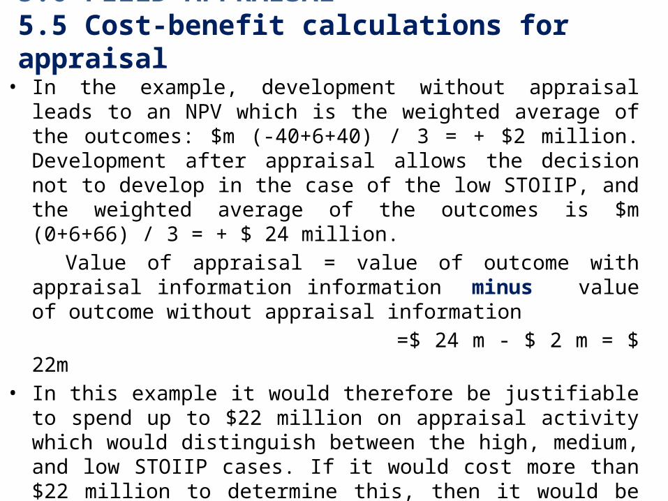
• In the example, development without appraisal leads to an NPV which is the weighted average of the outcomes: $m (-40+6+40) / 3 = + $2 million. Development after appraisal allows the decision not to develop in the case of the low STOIIP, and the weighted average of the outcomes is $m (0+6+66) / 3 = + $ 24 million.
Value of appraisal = value of outcome with appraisal information information minus value of outcome without appraisal information
=$ 24 m - $ 2 m = $ 22m
• In this example it would therefore be justifiable to spend up to $22 million on appraisal activity which would distinguish between the high, medium, and low STOIIP cases. If it would cost more than $22 million to determine this, then it would be better to go ahead without the appraisal. The decision tree has therefore been used to place a value on the appraisal activity, and to indicate when it is no longer worthwhile to appraise.
5.0 FIELD APPRAISAL5.5 Cost-benefit calculations for appraisal

• The benefit of using the decision tree approach is that it clarifies the decision-making process. The discipline required to construct a logical decision tree may also serve to explain the key decisions and to highlight uncertainties.
• The fiscal regime (or tax system) in some countries allows the cost of exploration and appraisal (E&A) activity to be offset against existing income as a fiscal allowance before the taxable income is calculated. For a taxpaying company, the real cost of appraisal is therefore reduced, and this should be recognised in performing the cost-benefit calculations.
5.0 FIELD APPRAISAL5.5 Cost-benefit calculations for appraisal

• In addition to the cost-benefit aspects of appraisal activities, there are frequently other practical considerations which affect appraisal planning, such as
• time pressure to start development (e.g. resulting from production sharing contracts which limit the exploration and appraisal period)
• the views of the partners in the block• availability of funds of operator and partners• increased incentives to appraise due to tax relief available on appraisal
• rig availability
5.0 FIELD APPRAISAL5.6 Practical aspects of appraisal

• Appraisal wells are often abandoned after the required data has been collected, by placing cement and mechanical plugs in the well and capping the well with a sealing device. If development of the field appears promising, consideration should be given to suspending the appraisal wells. This entails securing the well in an approved manner using safety devices which can later be removed, allowing the well to be used for production or injection during the field development. Approval must normally be given by the host
• government authority to temporarily suspend the well. Such action may save some of the cost of drilling a new development well, though in offshore situations the cost of re-using an appraisal well by later installing a subsea wellhead, a tie-back flowline and a riser may be comparable with that of drilling a new well.
5.0 FIELD APPRAISAL5.6 Practical aspects of appraisal

In locations where the addition of facilities for production is relatively cheap, phased development of a field may be an option. Instead of reducing the uncertainty to optimise the development plan before development starts, appraisal and development may be performed simultaneously. The results of appraisal during the early development are used to determine the next part of the development plan. This has the advantage of combining the data gathering with early production, which considerably helps the cash flow of a project
Phased development with simultaneous appraisal is more appropriate to onshore and shallow water developments, where facilities costs are lower. In deep water offshore developments, using single integrated drilling and production platforms, there is a much stronger incentive to get the facilities design correct at an early stage, since later additions and modifications are much more expensive
5.0 FIELD APPRAISAL5.6 Practical aspects of appraisal

•Gas reservoirs are produced by expansion of the gas contained in the reservoir. •The high compressibility of the gas relative to the water in the reservoir (either connate water or underlying aquifer) make the gas expansion the dominant drive mechanism. •Relative to oil reservoirs, the material balance calculation for gas reservoirs is rather simple.
•A major challenge in gas field development is to ensure a long sustainable plateau (typically 10 years) to attain a good sales price for the gas; the customer usually requires a reliable supply of gas at an agreed rate over many years.
•The recovery factor for gas reservoirs depends upon how low the abandonment pressure can be reduced, which is why compression facilities are often provided on surface.
• Typical recovery factors are in the range 50 to 80 %.
7.0 GAS RESERVOIR

• The main differences between oil and gas field development are associated with: The economics of transporting gasThe market for gasProduct specificationsThe efficiency of turning gas into energy
• Per unit of energy generated, the transportation of gas is significantly more expensive than transporting oil, due to the volumes required to yield the same energy.
• On a calorific basis approximately 6000 scf of gas is equivalent to one barrel (5.6 scf) of oil.
7.0 GAS RESERVOIR7.1 Major differences between oil and gas field development

• The compression costs of transporting gas at sufficient pressure to make transportation more economic are also high. This means that unless there are sufficiently large quantities of gas in the reservoir to take advantage of economies of scale, development may be uneconomic.
• For an offshore field, recoverable volumes of less than 0.5 trillion scf (Tcf) are typically uneconomic to develop. This would equate to an oil field with recoverable reserves of approximately 80 MMstb.
• When a customer agrees to purchase gas, product quality is specified in terms of the calorific value of the gas, measured by the Wobbe index (MJ/m3 or Btu/scf), the hydrocarbon dew point and the water dew point, and the fraction of other gases such as N2, CO2, H2S.
• H2S is undesirable because of its toxicity and corrosive properties. CO2 can cause corrosion in the presence of water, and N2 simply reduces the calorific value of the gas as it is inert.
7.0 GAS RESERVOIR7.1 Major differences between oil and gas field development
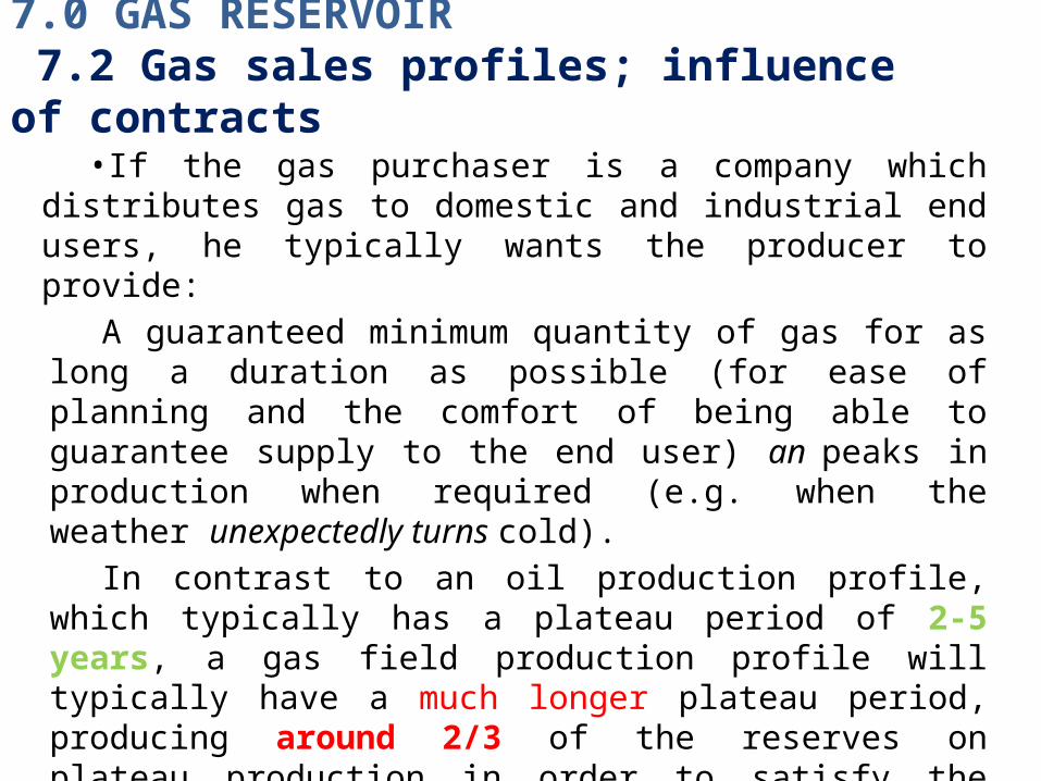
•If the gas purchaser is a company which distributes gas to domestic and industrial end users, he typically wants the producer to provide:
A guaranteed minimum quantity of gas for as long a duration as possible (for ease of planning and the comfort of being able to guarantee supply to the end user) an peaks in production when required (e.g. when the weather unexpectedly turns cold).
In contrast to an oil production profile, which typically has a plateau period of 2-5 years, a gas field production profile will typically have a much longer plateau period, producing around 2/3 of the reserves on plateau production in order to satisfy the needs of the distribution company to forecast their supplies. The Figure 39 compares typical oil and gas field production profiles.
7.0 GAS RESERVOIR 7.2 Gas sales profiles; influence of contracts

Figure 39: Comparison of typical oil and gas field production profiles
7.0 GAS RESERVOIR 7.2 Gas sales profiles; influence of contracts
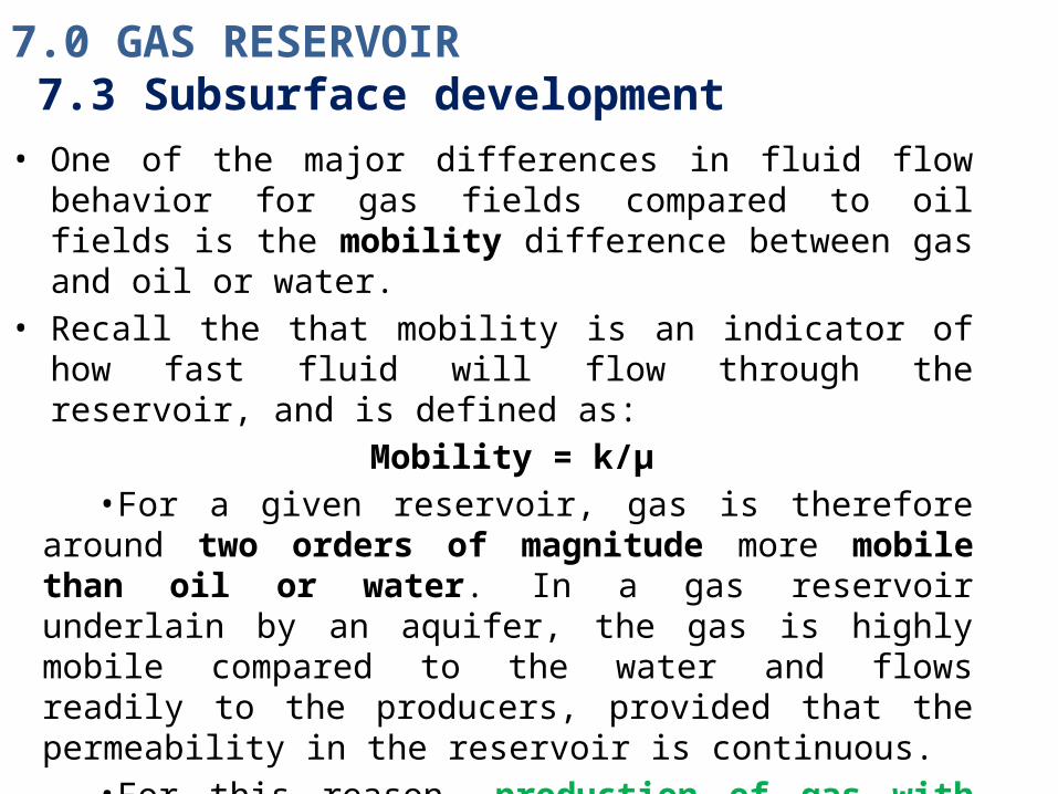
• One of the major differences in fluid flow behavior for gas fields compared to oil fields is the mobility difference between gas and oil or water.
• Recall the that mobility is an indicator of how fast fluid will flow through the reservoir, and is defined as:
Mobility = k/µ•For a given reservoir, gas is therefore
around two orders of magnitude more mobile than oil or water. In a gas reservoir underlain by an aquifer, the gas is highly mobile compared to the water and flows readily to the producers, provided that the permeability in the reservoir is continuous.
•For this reason, production of gas with zero water cut is common, at least in the early stages of development when the perforations are distant from the gas-water contact.
7.0 GAS RESERVOIR 7.3 Subsurface development

Location of wells•In a gas field development, producers are
typically positioned at the crest of the reservoir, in order to place the perforations as far away from the rising gas water contact as possible.
Movement of gas -water contact during production
•As the gas is produced, the pressure in the reservoir drops, and the aquifer responds to this by expanding and moving into the gas column.
•As the gas water contact moves up, the risk of coning water into the well increases, hence the need to initially place the perforations as high as possible in the reservoir.
7.0 GAS RESERVOIR 7.3 Subsurface development

Movement of gas -water contact during production
The above descriptions may suggest that rather few wells, placed in the crest of the field are required to develop a gas field. There are various reasons why gas field development requires additional wells:
The reservoir will not be homogeneous and certain areas will require closer well spacing to drain tighter parts of the reservoir in the same time as the more permeable areas are drained.
The reservoir may not be continuous and dedicated producers will be required to drain isolated fault blocks.
The reservoir may have a flat structure and therefore it may be impossible to place perforations at sufficient height above the water contact to avoid water coning. In this case, a lower production rate is necessary, implying more wells to meet the required production rate.
7.0 GAS RESERVOIR 7.3 Subsurface development
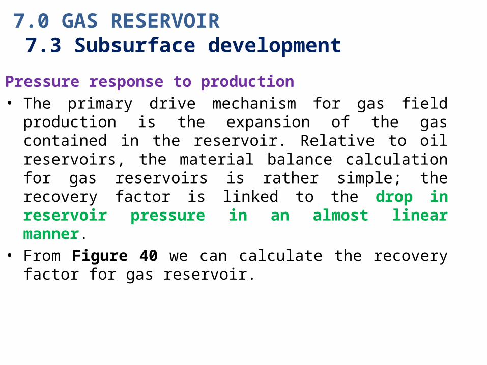
Pressure response to production• The primary drive mechanism for gas field production is the expansion of the gas contained in the reservoir. Relative to oil reservoirs, the material balance calculation for gas reservoirs is rather simple; the recovery factor is linked to the drop in reservoir pressure in an almost linear manner.
• From Figure 40 we can calculate the recovery factor for gas reservoir.
7.0 GAS RESERVOIR 7.3 Subsurface development

7.0 GAS RESERVOIR Pressure response to production
Figure 40: The "P over z" plot for gas reservoirs
The subscript "i" refers to the initial pressure, and the subscript "ab" refers to the abandonment pressure; the pressure at which the reservoir can no longer produce gas to the surface. If the abandonment conditions can be predicted, then an estimate of the recovery factor can be made from the plot. Gp is the cumulative gas produced, and G is the gas initially in place (GIIP).
Typical recovery factors for gas field development are in the range 50 to 80 percent, depending on the continuity and quality of the reservoir

7.0 GAS RESERVOIR Alternative uses for gas
A gas discovery may be a useful source of energy for supporting pressure in a neighbouring oil field, or for a miscible gas drive.
Selling the gas is not the only method of exploiting a gas field.
Gas reservoirs may also be used for storage of gas. For example a neighbouring oil field may be commercial to develop for its oil reserves, but the produced associated gas may not justify a dedicated export pipeline.
This gas can be injected into a gas reservoir, which can act as a storage facility, and possibly back produced at a later date if sufficient additional gas is discovered to justify building a gas export system.
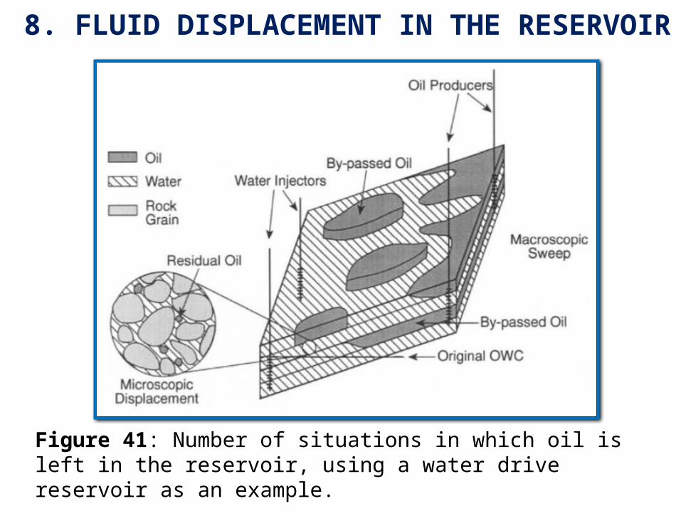
8. FLUID DISPLACEMENT IN THE RESERVOIR
Figure 41: Number of situations in which oil is left in the reservoir, using a water drive reservoir as an example.

8. FLUID DISPLACEMENT IN THE RESERVOIR
Figure 42: ‘Residual’ Saturation Distribution when displacing oil by water

Figure 43: Relative permeability curve for oil and water
kw = k* krw
Permeability water (kw) can be determined from the absolute permeability (k) and the relative permeability (krw) as follows:
8. FLUID DISPLACEMENT IN THE RESERVOIR

When water is displacing oil in the reservoir, the mobility ratio determines which of the fluids moves preferentially through the pore space. The mobility ratio for water displacing oil is defined as:
Mobility ratio (M) =(krw/µw)/(kro/µo)If the mobility ratio is greater than 1.0,
then there will be a tendency for the water to move preferentially through the reservoir, and give rise to an unfavourable displacement front which is described as viscous fingering. If the mobility ratio is less than unity, then one would expect stable displacement, as shown in Figure 44.
8. FLUID DISPLACEMENT IN THE RESERVOIR
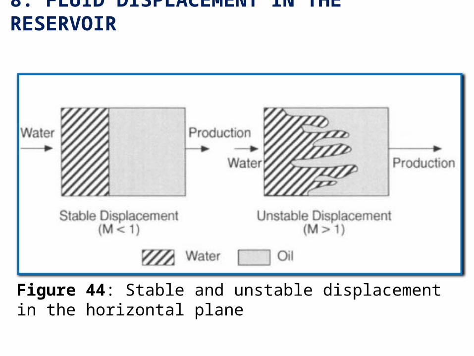
Figure 44: Stable and unstable displacement in the horizontal plane
8. FLUID DISPLACEMENT IN THE RESERVOIR

So far we have looked only at the viscous forces (which are a measure of the resistance to flow) acting on reservoir fluids.
Another important force which determines flow behaviour is the gravity force. The effect of the gravity force is to separate fluids according to their density.
During displacement in the reservoir, both gravity forces and viscous forces play a major role in determining the shape of the displacement front.
Consider the following example of water displacing oil in a dipping reservoir.
Assuming a mobility ratio less than 1.0, the viscous forces will encourage water to flow through the reservoir faster than oil, while the gravity forces will encourage water to remain at the lowest point in the reservoir.
8. FLUID DISPLACEMENT IN THE RESERVOIR

Figure 45: Gravity tonguing
8. FLUID DISPLACEMENT IN THE RESERVOIR
9.0 ESTIMATING THE RECOVERY FACTOR
Recall that the recovery factor (RF) defines the relationship between the hydrocarbons initially in place (HCIIP) and the ultimate recovery for the field.Ultimate Recovery = HCIIP * Recovery Factor [stb] or [scf]Reserves = UR - Cumulative Production [stb] or [scf] The main techniques for estimating the recovery factor are: field analogues analytical models (displacement calculations, material balance)
reservoir simulationField analogues should be based on reservoir rock type (e.g. tight sandstone, fractured carbonate), fluid type, and environment of deposition.
This technique should not be overlooked, especially where little information is available, such as at the exploration stage.
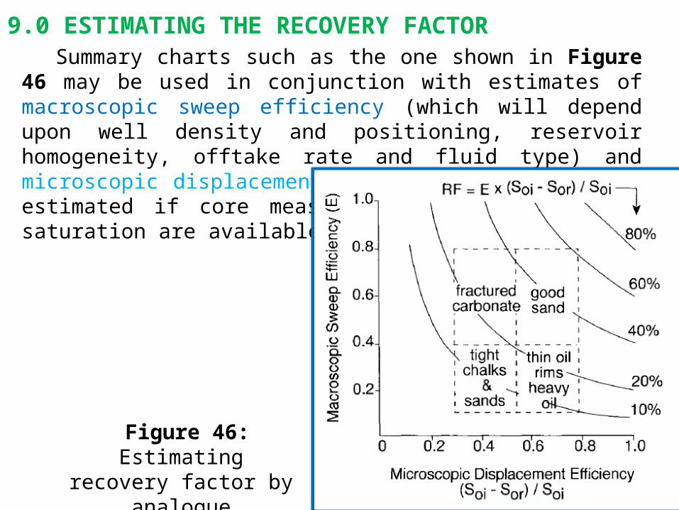
Summary charts such as the one shown in Figure 46 may be used in conjunction with estimates of macroscopic sweep efficiency (which will depend upon well density and positioning, reservoir homogeneity, offtake rate and fluid type) and microscopic displacement efficiency (which may be estimated if core measurements of residual oil saturation are available).
Figure 46: Estimating
recovery factor by analogue
9.0 ESTIMATING THE RECOVERY FACTOR

Analytical models using classical reservoir engineering techniques such as material balance, aquifer modeling and displacement calculations can be used in combination with field and laboratory data to estimate recovery factors for specific situations.
These methods are most applicable when there is limited data, time and resources, and would be sufficient for most exploration and early appraisal decisions.
However, when the development planning stage is reached, it is becoming common practice to build a reservoir simulation model, which allows more sensitivities to be considered in a shorter time frame.
9.0 ESTIMATING THE RECOVERY FACTOR
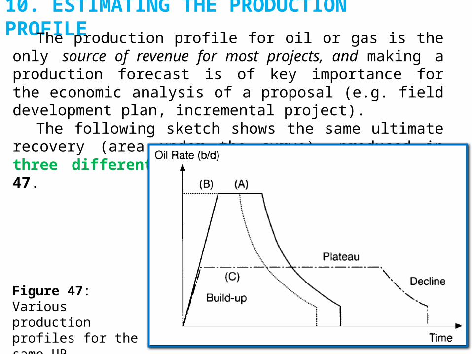
10. ESTIMATING THE PRODUCTION PROFILEThe production profile for oil or gas is the only source of revenue for most projects, and making a production forecast is of key importance for the economic analysis of a proposal (e.g. field development plan, incremental project).
The following sketch shows the same ultimate recovery (area under the curve), produced in three different production profiles in Figure 47.
Figure 47: Various production profiles for the same UR

In the build-up period, profile A illustrates a gradual increase of production as the producing wells are drilled and brought on steam; the duration of the build-up period is directly related to the drilling schedule. Profile B, in which some wells have been predrilled starts production at plateau rate.
The advantage of pre-drilling is to advance the production of oil, which improves the project cashflow, but the disadvantages are the that the cost of drilling has been advanced, and that the opportunity has been lost to gather early production information from the first few wells, which may influence the location of subsequent wells. Economic criteria (the impact on the profitability of the project) are used to decide whether to pre-drill.
10. ESTIMATING THE PRODUCTION PROFILE

The plateau production rates for cases A and B differ significantly from that in case C, which has a lower but longer plateau. The advantage of profile C is that it requires smaller facilities and probably less wells to produce the same UR.
This advantage in reduced costs must be considered using economic criteria against the delayed production of oil (which is bad for the cashflow). One additional advantage of profile C is that the lower Production rate, and therefore slower displacement in the reservoir, may improvethe UR.
10. ESTIMATING THE PRODUCTION PROFILE
Finally, external constraints on the production profile may arise fromproduction ceilings (e.g. OPEC production quotas)host government requirements (e.g. generating long period of stable income)customer demand (e.g. gas sales contract for 10 year stable delivery)production license duration (e.g. limited production period under a Production Sharing Contract)
10. ESTIMATING THE PRODUCTION PROFILE

11. ENHANCED OIL RECOVERYEnhanced oil recovery (EOR) techniques seek
to produce oil which would not be recovered using the primary or secondary recovery methods discussed so far. Three categories of enhanced oil recovery exist : thermal techniques; chemical techniques; miscible processes
Thermal techniques are used to reduce the viscosity of heavy crudes, thereby improving the mobility, and allowing the oil to be displaced to the producers.
This is the most common of the EOR techniques, and the most widely used method of heat generation is by injecting hot water or steam into the reservoir.
This can be done in dedicated injectors (hot water or steam drive), or by alternately injecting into, and then producing from the same well (steam soak).
A more ambitious method of generating heat in the reservoir is by igniting a mixture of the hydrocarbon gases and oxygen, and is called insitu combustion.

Chemical techniques change the physical properties of either the displacing fluid, or of the oil, and comprise of polymer flooding and surfactant flooding.
Polymer flooding aims at reducing the amount of by-passed oil by increasing the viscosity of the displacing fluid, say water, and thereby improving the mobility ratio (M).
Mobility ratio (M) =(krw/µw)/(kro/µo)This technique is suitable where the natural
mobility ratio is greater than 1.0. Polymer chemicals such as polysaccharides are added to the injection water.
Surfactant flooding is targeted at reducing the amount of residual oil left in the pore space, by reducing the interfacial tension between oil and water and allowing the oil droplets to break down into small enough droplets to be displaced through the pore throats.
Very low residual oil saturations (around 5%) can be achieved. Surfactants such as soaps and detergents are added to the injection water.
11. ENHANCED OIL RECOVERY

Miscible processes are aimed at recovering oil which would normally be left behind as residual oil, by using a displacing fluid which actually mixes with the oil.
Because the miscible drive fluid is usually more mobile than oil, it tends to bypass the oil giving rise to a low macroscopic sweep efficiency.
The method is therefore best suited to high dip reservoirs. Typical miscible drive fluids include hydrocarbon solvents, hydrocarbon gases, carbon dioxide and nitrogen.
11. ENHANCED OIL RECOVERY

Figure 48: Illustrate when considering secondary or enhanced oil recovery, it is important to establish where the remaining oil lies.
11. ENHANCED OIL RECOVERY

12.0 WELL DYNAMIC BEHAVIOURThe wells provide the conduit for production
from the reservoir to the surface, and are therefore the key link between the reservoir and surface facilities.
The type and number of wells required for development will dictate the drilling facilities needed, and the operating pressures of the wells will influence the design of the production facilities.
The application of horizontal or multi-lateral wells may where appropriate greatly reduce the number of wells required, which in time will have an impact on the cost of development.
Horizontal or multi-lateral wells can also be used to cost efficiently access remaining oil in mature fields.

12.0 WELL DYNAMIC BEHAVIOUR12.1 Estimating the number of development wells
The type and number of wells required for development will influence the surface facilities design and have a significant impact on the cost of development. Typically the drilling expenditure for a project is between 20 and 40% of the total CAPEX. A reasonable estimate of the number of wells required is therefore important.
When preparing feasibility studies, it is often sufficient to estimate the number of wells by consideringthe type of development (e.g. gas cap drive, water injection, natural depletion)the production/injection potential of individual wells

The number of producing wells needed to attain this profile can then be estimated from the plateau production rate and the initial production rates (well initial) achieved during the production tests on the exploration and appraisal wells.
12.0 WELL DYNAMIC BEHAVIOUR12.1 Estimating the number of development wells
No of production wells=plateau production rate [stb/d]assumed well initial [stb/d]

There will be some uncertainty as to the well initials, since the exploration and appraisal wells may not have been completed optimally, and their locations may not be representative of the whole of the field.
A range of well initials should therefore be used to generate a range of number of wells required.
The individual well performance will depend upon the fluid flow near the wellbore, the type of well (vertical, deviated or horizontal), the completion type and any artificial lift techniques used.
The number of injectors required may be estimated in a similar manner, but it is unlikely that the exploration and appraisal activities will have included injectivity tests.
Estimating the injection potential depended on an assessment of reservoir quality in the water column, which may be reduced by the effects of compaction and diagenesis.
12.0 WELL DYNAMIC BEHAVIOUR12.1 Estimating the number of development wells

Development plans based on water injection or natural aquifer drive, since appraisal activity to establish the reservoir properties in the water column is frequently overlooked. In the absence of any data, a range of assumptions of injectivity should be generated, to yield a range of number of wells required. If this range introduces large uncertainties into the development plan, then appraisal effort to reduce this uncertainty may be justified.
12.0 WELL DYNAMIC BEHAVIOUR12.1 Estimating the number of development wells

12.0 WELL DYNAMIC BEHAVIOUR12.1 Estimating the number of development wells

Figure 49: The presence of faults is another element that may change the number of injection/production wells required.
12.0 WELL DYNAMIC BEHAVIOUR12.1 Estimating the number of development wells

12.0 WELL DYNAMIC BEHAVIOUR12.2 Fluid flow near the wellbore
The pressure drop around the wellbore of a vertical producing well is described in the simplest case by the following profile of fluid pressure against radial distance from the well.
Figure 50: Pressure distribution around the wellbore

The difference between the flowing wellbore pressure (Pwf) and the average reservoir pressure reservoir pressure (P) is the pressure drawdown (∆ PDD). ∆PDD = Pa - Pwf [psi] or [bar]
The relationship between the flowrate (Q) towards the well and the pressure drawdown is approximately linear, and is defined by the productivity index (PI).
PI = Q/ ∆PDD [bbl/d/psi] or [m3/d/ bar]For an oil reservoir a productivity index of
1bbl/d/psi would be low for a vertical well, and a PI of 50 bbl/d/psi would be high.
12.0 WELL DYNAMIC BEHAVIOUR12.2 Fluid flow near the wellbore

The flowrate of oil into the wellbore is also influenced by the reservoir properties of:•permeability (k) and •reservoir thickness (h), •by the oil properties viscosity (µ) •and formation volume factor (Bo) and •by any change in the resistance to flow near the wellbore which is represented by the dimensionless term called skin (S)
12.0 WELL DYNAMIC BEHAVIOUR12.2 Fluid flow near the wellbore
The damage is caused by the invasion of solids from the drilling mud or from the cementing of the casing. The solid particles partially block the pore space and cause a resistance to flow, giving rise to an undesirable pressure drop near the wellbore. This so called damage skin.
Another common cause of skin is partial perforation of the casing across the reservoir which causes the fluid to converge as it approaches the wellbore, again giving rise to increased pressure drop near the wellbore. This component of skin is called geometric skin, and can be reduced by adding more perforations.
At very high flowrates, the flow regime may switch from laminar to turbulent flow, giving rise to an extra pressure drop, due to turbulent skin; this is more common in gas wells, where the velocities are considerably higher than in oil wells.
12.0 WELL DYNAMIC BEHAVIOUR12.2 Fluid flow near the wellbore

Figure 51: Pressure drop due to skinIn gas wells, the inflow equation which
determines the production rate of gas (Q) can be expressed as∆PDD = AQ + FQ2
The first term (AQ) is the pressure drop due to laminar flow, and the FQ 2 term is the pressure drop due to turbulent flow.
12.0 WELL DYNAMIC BEHAVIOUR12.2 Fluid flow near the wellbore

When the radial flow of fluid towards the wellbore comes under the Iocalised influence of the well, the shape of the interface between two fluids may be altered. The following diagrams show the phenomena of coning and cusping of water, as water is displacing oil towards the well.
Coning occurs in the vertical plane, and only when the otherwise stable oil-water contact lies directly below the producing well. Water is "pulled up" towards the perforations, and once it reaches the perforations, the well will produce at excessive water cuts.
Cusping occurs in the horizontal plane, that is the stabilised OWC does not lie directly beneath the producing well. The unwanted fluid, in this case water, is pulled towards the producing well along the dip of the formation.
12.0 WELL DYNAMIC BEHAVIOUR12.2 Fluid flow near the wellbore

The tendency for coning and cusping increases if:the flowrate in the well increasesthe distance between the stabilised OWC and the perforations reducesthe vertical permeability increasesthe density difference between the oil and water reduces
12.0 WELL DYNAMIC BEHAVIOUR12.2 Fluid flow near the wellbore

12.4 Production testing and bottom hole pressure testing
The production testing through the surface separator gathers information at surface. Another important set of information collected during bottom hole pressure testing is downhole pressure data, which is used to determine the reservoir properties such as permeability and skin. In a production well, which will have been completed with a production tubing and packer, the downhole pressure measurement is typically taken by running a pressure gauge, on wireline, to the depth of the reservoir interval. The downhole pressure gauge is then able to record the pressure while the well is flowing or when the well is shut in.
12.4 Production testing and bottom hole pressure testing
A static bottom hole pressure survey (SBHP) is useful for determining the reservoir pressure near the well, undisturbed by the effects of production. This often cannot be achieved by simply correcting a surface pressure measurement, because the tubing contents may be unknown, or the tubing contains a compressible fluid whose density varies with pressure (which itself has an unknown profile).
A flowing bottom hole pressure survey (FBHP) is useful in determining the pressure drawdown in a well (the difference between the average reservoir pressure and the flowing bottom hole pressure, Pwf) from which the productivity index is calculated.
By measuring the FBHP with time for a constant production rate, it is possible to determine the parameters of permeability and skin, and possibly the presence of a nearby fault
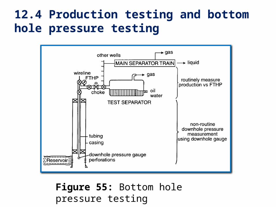
12.4 Production testing and bottom hole pressure testing
Figure 55: Bottom hole pressure testing

12.4 Production testing and bottom hole pressure testing
It is common practice to record the bottom hole pressure firstly during a flowing period (pressure drawdown test), and then during a shut-in period (pressure build-up test). During the flowing period, the FBHP is drawn down from the initial pressure, and when the well is subsequently shut in, the bottom hole pressure builds up.
Drawdown and build-up surveys are typically performed once a production well has been completed, to establish the reservoir property of permeability (k), the well completion efficiency as denoted by its skin factor (S), and the well productivity index (PI).

12.4 Production testing and bottom hole pressure testing
Figure 56: Pressure drawdown and build-up survey
12.4 Production testing and bottom hole pressure testing
In exploration wells which show hydrocarbon indications, it is often required to test the productivity of the well, and to capture a fluid sample. This can be used as proof of whether further exploration and appraisal is justified. If the well is unlikely to be used as a production well, a method of well testing is needed which eliminates the cost of running casing across the prospective interval and installing a production tubing, packer and wellhead. In such a case, a drill stem test (DST) may be performed using a dedicated drill string, called a test string, which has gas-tight seals at the joints.

12.4 Production testing and bottom hole pressure testing
Figure 57: Drill stem testing (DST)
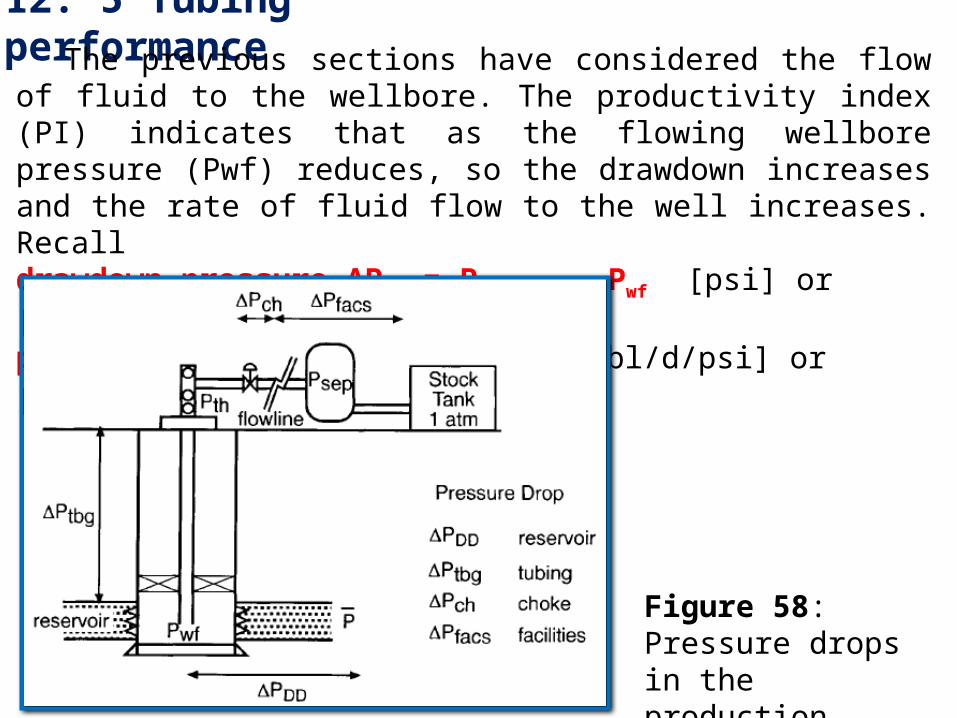
12. 5 Tubing performanceThe previous sections have considered the flow of fluid to the wellbore. The productivity index (PI) indicates that as the flowing wellbore pressure (Pwf) reduces, so the drawdown increases and the rate of fluid flow to the well increases. Recalldrawdown pressure ∆PDD = Paverage – Pwf [psi] or [bar]productivity index PI = Q/∆PDD [bbl/d/psi] or [m3/d/bar]
Figure 58: Pressure drops in the production process

12. 5 Tubing performance
The pressure drops in the production process can be split into three parts; the reservoir, the tubing and the surface facilities, with the linking pressures being the flowing wellbore pressure (Pwf) and the tubing head pressure (Pth).
To overcome the choke and facilities pressure drops a certain tubing head pressure is required.
To overcome the vertical pressure drop in the tubing due to the hydrostatic pressure of the fluid in the tubing and friction pressure drops, a certain flowing wellbore pressure is required.

Assuming for the moment a fixed required tubing head pressure, an equilibrium must exist between the reservoir performance (which delivers more fluid for lower values of Pwf) and the tubing performance (which delivers more fluid for higher values of Pwf)- This equilibrium is ensured by the correct selection of tubing size for the well, and depends upon the required tubing head pressure and the fluid type (GOR, BS&W).
The following diagram shows an example of the equilibrium between the inflow performance relationship (IPR) of the reservoir and the tubing performance curve (TPC) for two tubing sizes.
12. 5 Tubing performance

12. 5 Tubing performance
Figure 59: Reservoir performance and tubing performance

12. 5 Tubing performance
For the reservoir with IPR 1, the larger tubing does not achieve an equilibrium, and the well would not flow if the 51/2" tubing was installed. However, a different reservoir with IPR 2 would benefit from a larger tubing size which would allow greater production, and the correct selection of tubing size would be the 51/2" tubing if one wanted to maximise the early production from the well.
An understanding of the tubing performance (which can be predicted) and the reservoir performance (which requires reservoir data gathering) is important for the correct selection of tubing size.

12. 5 Tubing performance
The end of field life is often determined by the lowest reservoir pressure which can still overcome all the pressure drops described and provide production to the stock tank. As the reservoir pressure approaches this level, the abandonment conditions may be postponed by reducing some of the pressure drops, either by changing the choke and separator pressure drops as mentioned, or by introducing some form of artificial lift mechanism.
In gas field development, the recovery factor is largely determined by how low a reservoir pressure can be achieved before finally reaching the abandonment pressure.

12.6 Well completionsWhen a production or injection well is
drilled, it is common practice to cement in place a casing which extends across the reservoir interval. The alternative is to leave the reservoir uncased, in a so-called bare foot completion, which is rarely done. When the drilling department finishes its work on the well, it is often left in the state of a cased hole, as on the left of Figure 60.The figure on the right shows the well with a simple well completion including a production tubing with packer, a series of surface safety valves called a Christmas tree, a subsurface safety valve (SSSV), a circulating sleeve, and a series of perforations through the casing.

The purpose of the weft completion is to provide a safe conduit for fluid flow from the reservoir to the flowline. The perforations in the casing are typically achieved by running a perforating gun into the well on electrical wireline. The gun is loaded with a charge which, when detonated, fires a high velocity jet through the casing and on into the formation for a distance of around 15-30 cm. In this way communication between the wellbore and the reservoir is established. Wells are commonly perforated after the completion has been installed and pressure tested.
12.6 Well completions
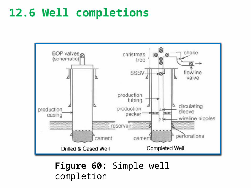
Figure 60: Simple well completion
12.6 Well completions
During production, the tubing may be exposed to corrosive and erosive fluids, and may need to be replaced before the end of the field lifetime. This is another safety feature of the completion; a corroded or eroded tubing can be safely replaced during a workover.
If it were the casing that had become damaged during production, this could not be removed, and a major well repair or even abandonment might have been the result.
Well completions are usually tailored to individual wells, and many variations exist.
The following diagrams show a completion with a gravel pack, designed to exclude sand production downhole, and a dual completion, designed to allow controlled production from two separate reservoirs.
12.6 Well completions

Figure 61: Gravel pack completion and dual completion
12.6 Well completions

In the internal gravel pack shown, carefully sorted sand grains, called gravel, are placed between a wire wrapped screen and the perforations with the objective of stopping loosely consolidated reservoir sand from being produced into the wellbore. The dual completion is useful in controlling the offtake from two separate reservoirs, and allows the production from each reservoir to be monitored independently. The alternative would be to produce both reservoirs through a single production tubing in commingled production.
Completions in horizontal wells are also tailored to the individual reservoir.
The bare foot completion, which leaves an open hole section below the previous casing, is cheap, simple and suitable for consolidated formations which have little tendency to collapse.
12.6 Well completions

The slotted finer is an uncemented section of casing with small intermittent slots cut along its length, which prevents the hole from collapsing, but allows no selectivity of the interval which will be produced.
The cased and cemented horizontal completion does allow a choice of which intervals will be perforated and produced. None of these examples provides any effective sand exclusion; if this is required a gravel pack or a pre-packed liner can be used.
12.6 Well completions
Figure 61: Horizontal well completions

12.7 Artificial liftSome wells may simply flow more efficiently
on artificial lift, others require artificial lift to get started and will then proceed to flow on natural lift, others yet may not flow at all on natural flow.
In any of these cases, the cost of the artificial lift system must be offset against the gains. In clear cut cases, such as on-shore stripper wells where the bulk of the operating costs are the lifting costs, the problem can be quite transparent.
Artificial lift systems are mostly required later in a field's life, when reservoir pressures decline and therefore well productivities drop.
If a situation is anticipated where artificial lift will be required or will be cost effective later in a field's life, it may be advantageous to install the artificial lift equipment up front and use it to accelerate production throughout the field's life, provided the increased revenues from the accelerated production offset the cost of the earlier investment.

In other cases it may be beneficial to install multiple artificial lift systems to cater for different wells, or to change the artificial lift system in the life of the well to cater for the different operating conditions.
Typical examples are wells that are converted to ESP (Electrical Submersible Pump) lift later in life as watercut increases.
The following types of artificial lift are commonly available today:
Gas Lift Electric Submersible Pump (ESP) Beam Pump (Sucker Rod Pump) Jet (Venturi) Pump Progressing Cavity Pump (PCP) Plunger Lift Hydraulic Lift
12.7 Artificial lift

Artificial Lift Operating Constraints (1)Sucker rod pump Progressing
cavity pumpGas lift
Maximum operating depth, ft TVD
16,000 6,000 15,000
Operating fluid volume, bbl/day
20 – 5,000 5 – 4,500 250 – 30,000
Maximum operating temperature, oF
550 250 400
Corrosion handling
Good to excellent Fair to good Good to excellent
Gas handling Fair to good Good ExcellentSolids handling Fair to good Excellent Good to excellentFluid gravity, oAPI
> 8 < 35 > 15
Servicing Workover or pulling rig
Workover or pulling rig
Wireline or workover rig
Wellbore deviation
0 – 90o landed pump; 15o/100ft build angle
0 – 90o landed pump; 15o/100ft build angle
0 – 70o short to medium radius
Prime mover Gas or electric Gas or electric CompressorOffshore application
Poor Good Excellent
Gas/liquid ratio, scf/bbl/1,000ft depth
- - -

Plunger lift Hydraulic lift Electric submersible pump
Maximum operating depth, ft TVD
14,000 17,000 (piston)15,000 (jet)
15,000
Operating fluid volume, bbl/day
50 – 200 50 – 4,000 (piston)300 – > 15,000 (jet)
200 – 30,000
Maximum operating temperature, oF
500 500 400
Corrosion handling Excellent Good to excellent Good
Gas handling Excellent Fair to good Poor to fair
Solids handling Poor to fair Poor to good Poor to fair
Fluid gravity, oAPI
- > 8 > 10
Servicing Wellhead catcher or wireline
Hydraulic or wireline Workover or pulling rig
Wellbore deviation 80o 0 – 90o pump placement; <15o/100ft build angle
(piston)>24o/100ft build angle
(jet)
0 – 90o pump placement,
<10o build angle
Prime mover Well’s natural energy
Multicylinder or electric
Electric motor
Offshore application
N/A Good to excellent Excellent
Gas/liquid ratio, scf/bbl/1,000ft depth
400 - -
Artificial Lift Operating Constraints (2)
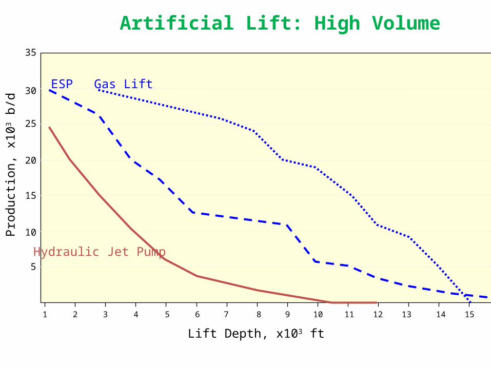
35
30
25
20
15
10
5
Prod
uction
, x1
03 b
/d
1 2 3 4 5 6 7 8 9 10 11 12 13 14 15 16
Lift Depth, x103 ft
Hydraulic Jet Pump
ESP Gas Lift
Artificial Lift: High Volume

Artificial Lift: Low Volume4.5
4.0
3.5
3.0
2.0
1.5
0.5
Barr
els pe
r day,
x10
3
1 2 3 4 5 6 7 8 9 10 11 12 13 14 15 16
2.5
1.0Progressing cavity pump
Sucker rod lift
Reciprocating hydraulic
Lift Depth, x103 ft

Gas Lift Equipment
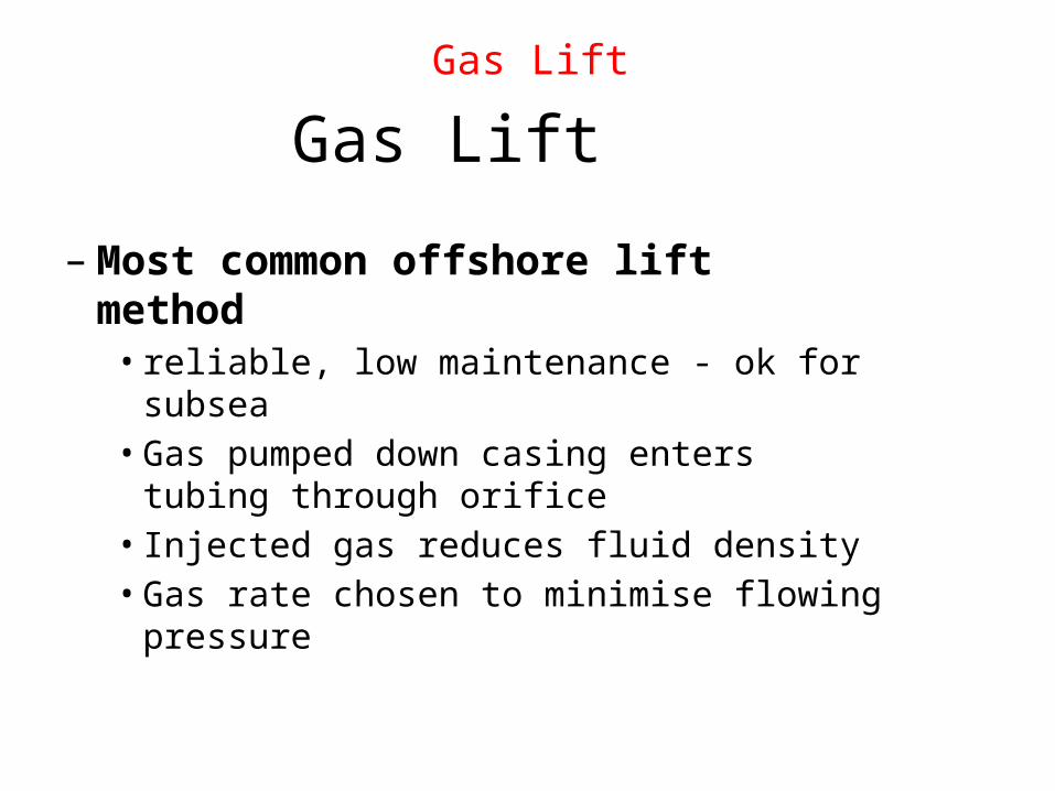
– Most common offshore lift method•reliable, low maintenance - ok for subsea
•Gas pumped down casing enters tubing through orifice
•Injected gas reduces fluid density•Gas rate chosen to minimise flowing pressure
Gas LiftGas Lift

Gas injection
Maximum Production
‘Optimum’ Injection
Prod
ucti
on Rat
e
Gas Lift Injection Rate
Well
Depth
Pressure
Gas Lift Principles

Electric Submersible Pump (ESP)

Motor Pump
ESP Equipment
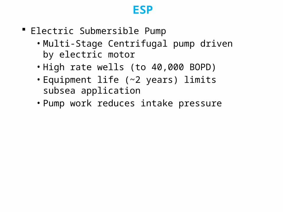
Electric Submersible Pump• Multi-Stage Centrifugal pump driven by electric motor
• High rate wells (to 40,000 BOPD)• Equipment life (~2 years) limits subsea application
• Pump work reduces intake pressure
ESP

ESP Flowing Gradient
0 900 1800 2700 360012000
9000
6000
3000
0
Pressure (psig)
Meas
ured
Dep
th
(fee
t)
0 1 2
Pump Depth
Pump Power Increases
Pressure Boosted by Pump
Artificial Lift Operating Constraints (1)

Electric Submersible Pump (ESP)Failure Analysis

95 96 97 98 99Dec Jan Feb Mar Apr May Jun Jul Aug Sep Oct Nov Dec Jan Feb Mar Apr May Jun Jul Aug Sep Oct Nov Dec Jan Feb Mar Apr May May Jun Jul Aug Sep Oct Nov Dec
D1#1 412D1#2 136D1#3 165
D2#1 282D2#2 437
D5#1 379D5#2 121D5#3 168
D7#1 492D7#2 18
D8#1 285D8#2 144D8#3 16D8#4 44D8#5 3D8#6 113
D11#1 365D11#2 3D11#3 243D11#4 101
D12#1 440D12#2 172
D15#1 318
D16#1 25
Days Run Electrically Available Switch over made to 3200 V tappings
Liverpool Bay Electric Submersible PumpsRun Life History

0
10000
20000
30000
40000
50000
60000
70000Oc
t-97
Nov-
97
Dec-
97
Jan-98
Feb-98
Mar-
98
Apr-98
May-98
Jun-98
Jul-98
Aug-98
Sep-98
Oct-98
Nov-98
Dec-98
Liverpool Bay Electric Submersible PumpsImpact on Oil Production
bopd
Timeline
Expected Production Level
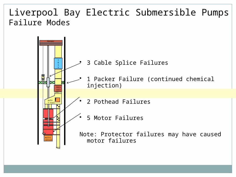
Hanger
TRSV
FBIVswivel
autoY-tool
multisensor
• 3 Cable Splice Failures
• 1 Packer Failure (continued chemical injection)
• 2 Pothead Failures
• 5 Motor Failures
Note: Protector failures may have caused motor failures
Liverpool Bay Electric Submersible PumpsFailure Modes

Critical factor was increasing power to pumps:• Increased production requirements• Increased off take, increased frequency, increased voltage, reduced intake pressure
Voltage V's Run Days Of Failed ESP's
0
100
200
300
400
2200-2800 3200Voltage
Days
Liverpool Bay Electric Submersible PumpsFailure Modes

• Electrical stress measured and reduced
– Monitoring of harmonics– Reduction of voltage
• Improved electrical robustness– Main power cable changed from
polypropylene to EPDM – Splice length increased to
allow application of additional insulation tape
– Power cable increased from 4KV to 5KV
– Low voltage high current motors
• Improved mechanical integrity– Changed protector
configuration– Introduced tandem protectors– Crimp connectors at pothead
replaced with bucket connectors
Hanger
TRSV
FBIVswivel
autoY-tool
multisensor
Liverpool Bay Electric Submersible PumpsImprovements Implemented

Beam Pump(Sucker Rod Pump)
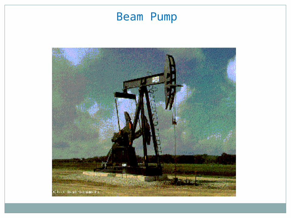
Beam Pump
‘Nodding Donkey’ pump Lowers BHP by lifting fluid in tubing Most common artificial lift method
Simple downhole plunger pump operated from surface via string of ‘sucker rods’
Low rate wells (20 BOPD up to ~4000 BOPD) Suitable for land operations (weight, maintenance)
Beam Pump

Sucker Rod Pump Production (bbl/day) Constants (1)Plunger diameter,
in.Cross-sectional plunger
area, sq. in.“C” pump constant
1 – 1/16 0.8866 0.13161 – 1/4 1.2272 0.18211 – 1/2 1.7671 0.26221 – 3/4 2.4053 0.3569
1 – 25/32 2.4900 0.36952 3.1416 0.4662
2 – 1/4 3.9671 0.59012 – 1/2 4.9087 0.72852 – 3/4 5.9396 0.88143 – 1/4 8.2958 1.23103 – 3/4 11.045 1.63904 – 3/4 17.721 2.6297

Efficiency expectations: tubing pump = 75% insert pump = 80%Formula: q = C x Sp x N x Ev
where: q = fluid production, bbl/dayC = pump constant = 0.1484 Ap
Ap = cross-sectional plunger area, sq. in.Sp = effective plunger stroke, in.N = pumping speed, strokes/minuteEv = volumetric efficiency
Sucker Rod Pump Production (bbl/day) Constants (2)
Formula: V = Cedp
where:V = m3/day/rpmC = 5.7 E-6
d = rotor minor diameter, mm
e = eccentricity, mmp = stator pitch, mm

EXERCISE
Copyright © 2022 FDOKUMEN