OF SJAN 14 993U - DTIC
346
AD-A259 231 OF SJAN 14 993U An Object-Oriented Computer Aided Design Program for Traditional Control Systems Analysis THESIS Wayne E. Bell, KLT. USAF --- , AFIT/GE/ENG/92D-03 ___ -u1 DEPARTMENT OF THE AIR FORCE AIR UNIVERSITY AIR FORCE INSTITUTE OF TECHNOLOGY Wright-Patterson Air Force Base, Ohio 93 1 08 040
-
Upload
khangminh22 -
Category
Documents
-
view
2 -
download
0
Transcript of OF SJAN 14 993U - DTIC

AD-A259 231
OF SJAN 14 993UAn Object-Oriented
Computer Aided Design Programfor
Traditional Control Systems Analysis
THESIS
Wayne E. Bell, KLT. USAF--- ,
AFIT/GE/ENG/92D-03 ___
-u1
DEPARTMENT OF THE AIR FORCE
AIR UNIVERSITY
AIR FORCE INSTITUTE OF TECHNOLOGY
Wright-Patterson Air Force Base, Ohio
93 1 08 040
AFIT/GE/ENG/92D-03
An Object-OrientedComputer Aided Design Program
forTraditional Control Systems Analysis
THESIS
Wayne E. Bell, 1LT, USAF
AFIT/GE/ENG/92D-03
Approved for public release; distribution unlimited
AFIT/GE/ENG/92D-03
An Object-OrientedComputer Aided Design Program
forTraditional Control Systems Analysis
THESIS
Presented to the Faculty of the School of Engineeringof the Air Force Institute of Technology
Air UniversityIn Partial Fulfillment of the
Requirements for the Degree ofMaster of Science in Electrical Engineering
Wayne E. Bell, B.S.1LT, USAF :;;;8ion For
NTIS GRA&I 1" 'December 1992 DTIC TAB 0
Unannou~noed 00Justi fication
By
Dstribution/Availability Codes
Avail and/orDist Spooial
Approved for public release; distribution unlimited
" "I) 7L
Preface
When I began doing homework in the controls sequence here at AFIT, it quickly
became obvious that all work had to be done on a computer. The complexity of the available
software became obvious just as quickly. MatLab, Matrixx, and Mathmatica were all available,
but only on the Sun workstations at school, and they weren't very user friendly. ICECAP-PC
quickly became the program of choice because of its user friendly interface and its availability
on home computers. However, ICECAP-PC's shine began to tarnish as the coursework became
more advanced and ICECAP-PC proved to be highly unreliable and underpowered.
Being a programmer from way back, I took it upon myself to be the champion of the
Class of '92 and began debugging ICECAP-PC. What began as an interest became an
obsession and grew into the scope of an entire thesis. ICECAP-PC was really the perfect
thesis topic for me. My primary sequence is Digital Engineering and my secondary sequence
is Digital Controls. The algorithms, literature reviews, example problems, etc. associated with
working on ICECAP-PC provided a remarkable education in both Digital Engineering and
Controls. And extending ICECAP-PC into the QFT toolboxes provided an opportunity to learn
some things beyond just traditional control algorithms.
ICECAP-PC version 10 represents the extent of the work I and Fred Trevino have been
able to achieve in bringing ICECAP-PC into the 21st Century. I only hope that thesis workers
will follow us sooner than we followed our predecessors. The longer the code is left without
thesis students, the harder it is for the new students to bring it back up to speed with current
technology. However, we have provided ICECAP-PC thesis students with an object-oriented,
algorithmically sound foundation for at least five years of adding new toolboxes. This means
that follow-on students can add toolboxes for LQG, Kalman filtering, Butterworth filter
templates, Lag-Lead controller design, discrete QFT, nonlinear QFT, etc. before any of them
have to worry about porting to the latest language. My guess is that the next port will be to
ii

a Microsoft Windows environment that is hosted within a 64-bit operating system (no 640K
barrier due to DOS). This is fully possible using the new Borland PASCAL 7.0. Whatever
ICECAP-PC's future code development holds, I firmly believe students are better off using
ICECAP-PC than they are using the commercial packages. ICECAP-PC teaches the process
more than just spitting out a computer generated answer.
I would like to thank Dr Horowitz for his many pearls of wisdom on both life and QFT.
It is indeed an honor to have such an esteemed man of history as part of my thesis committee.
I also thank Dr Houpis for being another controls powerhouse on my committee. I especially
want to mention his work in putting together the QFT Symposium. That symposium and the
Proceedings had to be the single largest contributor to my education in QFT. And to meet the
people whose names were on all the papers and texts I have read was truly significant.
And now for a man who deserves his own paragraph on this page of personal salutes:
Dr Lamont. Never again should such a respectable professor have to persevere such an
obnoxious thesis student as I. As much as Fred is every professors wet dream, I am the
nightmare that wakens them at night in a cold sweat. Thank you, Dr Lamont, for being a
helluva guy to hang around at OktoberFests and for being just as helluvan educator. P.S. If
you ever add any FORTRAN code to our beautiful PASCAL, I'll come back for a PhD!
On a personal level, I thank my wife Donna for living through all the nights the tippy-
tapping on the keyboard kept her awake till dawn. And I thank her for all those other nights
she was awake till dawn. I also thank my venerable thesis buddy, Fred-dude. Bravo for his
understanding of object-oriented code, matrix algorithms, and loud-mouthed lieutenants
("kids"). Don't you all just love old guys?
Wayne E. Bell
111ii
Table of Contents
Introduction .................................................. 11.1 History of CACSD ...................................... 11.2 History of ICECAP-PC ................................... 31.3 General Objectives ...................................... 4
1.3.1 The Object-Oriented CACSD Environment ............. 51.3.2 The Refinement Of Numerical Methods ............... 51.3.3 Toolboxes ....................................... 6
1.4 Report Organization .................................... 71.5 Sum m ary ............................................. 8
2 Technical Review .............................................. 92.1 Object-Oriented Design Discussion and Terminology ............ 10
2.1.1 Terminology ................................... 112.1.2 The OOD Process ................................ 172.1.3 Borland Turbo Vision ............................. 202.1.4 Advantages of OOP Over Functional Programming ...... 252.1.5 Disadvantages of OOP Over Functional
Programming ................................... 282.1.6 Summary of OOD and OOP ........................ 29
2.2 Literature Review of Human Interface Design ................. 302.2.1 ICECAP-PC 9.0 ................................ 312.2.2 Human Factors Engineering ....................... 342.2.3 Commercial Packages ............................ 382.2.4 CACSD Packages ................................ 422.2.5 Summary of User Interfaces ....................... 45
2.3 Literature Review of the Quantitative Feedback Theory .......... 452.3.1 The Design Problem ............................. 452.3.2 The Design Approach ............................. 462.3.3 The Design Procedure ............................ 462.3.4 Summary of QFT ................................ 47
2.4 Sum m ary ............................................. 47
3 Requirements and Specifications ................................... 493.1 General Traits ......................................... 50
3.1.1 Accuracy ...................................... 503.1.2 Speed ........................................ 503.1.3 Reusability .................................... 513.1.4 Portability ..................................... 513.1.5 Accessibility .................................... 523.1.6 Graphics Presentation ............................. 523.1.7 Intuitive Interface ............................... 53
3.2 Programming Standards .................................. 543.3 Mathematical Specification ............................... 56
iv
3.4 Human Interface Specification ............................. 593.4.1 Menuing System ................................ 593.4.2 On-Line Help ................................... 603.4.3 Data Display ................................... 60
3.5 Sum m ary ............................................. 61
4 Design and Implementation - ICECAP-PC ........................... 624.1 PASCAL .............................................. 624.2 Object-Orientation ...................................... 64
4.2.1 M odularity ..................................... 644.2.2 Independence ................................... 644.2.3 Testability ..................................... 654.2.4 Reliability ..................................... 65
4.3 ICECAP-PC 9.0 to ICECAP-PC 9.OA ........................ 654.3.1 Fast Prototyping ................................ 664.3.2 Unit Decomposition .............................. 664.3.3 Validating the Code .............................. 67
4.4 ICECAP-PC 9.OA to ICECAP-PC 10 ......................... 674.4.1 Variable Names ................................. 704.4.2 Data Structures ................................. 714.4.3 Global Records .................................. 744.4.4 Object Support .................................. 794.4.5 Error Handling Routines .......................... 824.4.6 Algorithm Improvement ........................... 834.4.7 Unit Decomposition .............................. 874.4.8 Compiler/Memory Issues .......................... 88
4.5 User Interface Development ............................... 904.5.1 The Menuing System ............................. 904.5.2 Number Format ................................. 954.5.3 User Configuration Files .......................... 964.5.4 On-Line Help System ............................ 964.5.5 Data Presentation ............................... 97
4.6 Summ ary ............................................ 100
5 Toolbox Design and Implementation - MISO QFT ..................... 1015.1 The Toolbox Concept ................................... 1015.2 The MISO QFT Toolbox ................................. 1025.3 The MISO Process ..................................... 1035.4 Code Development ..................................... 109
5.4.1 The MISO Data Structure ........................ 1095.4.2 The MISO Object ............................... 111
5.5 User Interface Development .............................. 1115.5.1 The MISO Menu Structure ....................... 1115.5.2 Interactive Graphics ............................ 111
5.6 Summ ary ............................................ 113
v
6 Testing and Validation ......................................... 1156.1 Black Box Testing ..................................... 1156.2 M acro File Object ...................................... 1166.3 W hite Box Testing ..................................... 1176.4 User Requests ........................................ 1226.5 MIMO QFT and LQR/LQG Example ........................ 1226.6 The Root Finder ....................................... 1236.7 Sum m ary ............................................ 124
7 Conclusions and Recommendations ................................ 1267.1 Conclusions .......................................... 126
7.1.1 General Objectives .............................. 1277.1.2 General Traits ................................. 1277.1.3 Programming Standards ......................... 1287.1.4 Mathematical Specifications ...................... 1287.1.5 Human Interface Specifications .................... 128
7.2 Recommendations ...................................... 1297.2.1 Error Handling Routine .......................... 1307.2.2 Database Object ................................ 1307.2.3 The Root Finder ............................... 1327.2.4 Multiple Windows .............................. 1327.2.5 Interactive Graphics ............................ 1337.2.6 Interactive Tracking Specification Generation ......... 1347.2.7 Augmented Model Bound Generation ................ 1347.2.8 Interface to Commercial Packages .................. 1357.2.9 System Build Toolbox ........................... 1367.2.10 Discrete Toolboxes .............................. 1367.2.11 Nonlinear Toolbox .............................. 1367.2.12 Time Delay Toolbox ............................. 1377.2.13 Transcendental Functions Toolbox .................. 137
7.3 Summary ............................................ 138
Appendices ......................................................... 139Appendix A Bibliography ...................................... 140Appendix B Testing and Validation .............................. 141Appendix C ICECAP-PC User's Manual ........................... 142Appendix D ICECAP-PC Programmer's Manual ..................... 143Appendix E QFT Toolbox User's Manual .......................... 144
vi
List of Figures
Figure 1 MISO QFT System Model ...................................... 45
Figure 2 The ICECAP-PC menuing system, button bar, and status bar ............ 91
Figure 3 A pull down menu example ..................................... 92
Figure 4 A dialog box example .......................................... 93
Figure 5 An example help window ....................................... 96
Figure 6 A log file example ............................................ 98
Figure 7 The full screen editor .......................................... 99
Figure 8 Stability bound generation ..................................... 106
Figure 9 Resulting roots given 1 / (82 + as + b), 1<a<5, 1<b<5 ................. 107
Figure 10 Convex Hull violation by ill-behaved bound ........................ 109
Figure 11 The MISO QFT Toolbox menu .................................. 112
vii
List of Listings
Listing 1 Basic Inheritance ............................................. 15
Listing 2 Abbreviated Turbo Vision Family Tree ............................. 21
Listing 3 Hypothetical DSP Object Cless .................................. 22
Listing 4 Event Handler For Hypothetical DSP Object ........................ 24
Listing 5 Internal Procedure Format ...................................... 55
Listing 6 Embedded Debugging Code ..................................... 55
Listing 7 Temporarily Commenting Out Code ............................... 55
Listing 8 Desired Mathematical Capabilities for ICECAP-PC ................... 58
Listing 9 The Extended Complex Data Structure ............................ 72
Listing 10 The Polynomial Data Structures ................................. 73
Listing 11 The Transfer Function Record ................................... 74
Listing 12 The Time Response data structure ................................ 76
Listing 13 The Frequency Response data structure ............................ 77
Listing 14 The Graphics data structure .................................... 79
Listing 15 MISO data structures ........................................ 110
Listing 16 Original IsZero function ....................................... 119
Listing 17 Second IsZero function ........................................ 120
Listing 18 Third IsZero function ......................................... 121
Listing 19 IsZero function with local ABSOL function ......................... 121
Listing 20 Possible Numerical Definitions .................................. 133
viii
Abstract
This thesis is a continuation of the ICECAP-PC research project conducted under Prof.
Gary B. Lamont at the Air Force Institute of Technology. It is an ongoing development of a
public domain Computer Aided Design package for Control Engineering and Digital Signal
Processing students, faculty and practitioners with a special emphasis on education.
This investigation begins with the software maintenance task of restructuring,
debugging, and testing the functional version of ICECAP-PC 9.0. This is done for both
transfer function and matrix portions of the package as well as continuous and discrete
portions. The continuous, traditional portions are then ported to a new object-oriented
program structure which is the primary focus of this effort. New interactive graphics
capabilities are then added as well as new procedures for the time and frequency response
plots. All basic math algorithms are rewritten to be more accurate within a contemporary
personal computer environment. All algorithms are optimized for speed, performance, and
memory requirements on personal computers. A new user-programmable macro file capability
is then designed and implemented to assist in the black box testing of the new code. Finally,
using a program extension concept called a toolbox, a Multiple-Input-Single-Output (MISO)
Quantitative Feedback Theory (QFT) toolbox is created. This toolbox allows manual,
interactive, and automatic QFT design for continuous, linear, time invariant MISO control
system problems.
ix
An Object-OrientedComputer Aided Design Program
forTraditional Control Systems Analysis
1 Introduction
Computer Aided Control System Design (CACSD) software development is a-I
inherently complex process because of (1) the multitude of mathematical operations and
capabilities required, and (2) the variety of requirements posed by the end users. Most
programs today are modular in structure and tasks are compartmentalized into functional
procedures (subroutines). User commands given are processed through a hierarchical tree of
procedures until the commanded function is fully executed. Relatively new, and growing
rapidly, is the use of object-oriented programming (OOP) techniques. While the software
engineering community embraces this technique with open arms, other engineering disciplines,
control systems engineering included, have been slow to adopt this technology. This is
unfortunate since object-orientation provides an ideal structure for CACSD program design,
because structural complexities are elegantly resolved. This thesis will break new ground in
applying OOP to CACSD software.
This chapter will introduce this topic by presentuig a history of CACSD development,
then a history of ICECAP-PC development, and finally the goals of this thesis effort.
1.1 History of CACSD [Iheir, 19881
The evolution of CACSD directly follows the evolution of control system theory itself.
The defense industry has been the major driving force in the development of automatic control
systems since World War II as increasingly sophisticated weapon systems have been needed.
In the period between 1930 to 1950, the largest category of problems was the SISO (Single-
Input Single-Output) systems, and design was predominantly performed in the frequency
domain. Prominent figures were W. R. Evans and H. Nyquist. Early control system problems
were solved without the aid of computers, and only simple cases (by today's standards) could
be considered.
As systems became more complex and MIMO (Multiple-Input Multiple-Output)
problems were presented, the frequency domain graphical techniques of the earlier decades
failed to produce solutions. Among others, R. Kalman led engineers into the time domain
where systems were represented in state space by a set of first-order differential equations in
place of nth-order ordinary differential equations. Concurrent with these developments was
the advent of the computer age. Engineers began producing code to solve very specific
problems. However, there was no single collection of routines unified under a single package
until the late seventies. [Dongarra, 1979; O'Brian, 1977; Smith, 19761 In the early days of
computing, the largest obstacle was the lack of interactive systems. Programs were placed on
punch cards and run in batch mode--a process that was extremely time consuming.
In the early seventies, researchers began to again look at the frequency domain for
control systems solutions, and diversification of theory began to rapidly take place. Different
approaches were presented for different classes of problems. Concurrent with these
developments, was the development of collections of routines, each being developed for a
specific purpose. In 1977, Fredrick L. O'Brian in his masters thesis at the Air Force Institute
of Technology developed the Consolidated Computer Program for Control System Design which
was a collection of these routines. [O'Brian, 19771 In 1978, follow on work at AFIT produced
TOTAL, recogr ad as the first interactive CACSD program. In 1979, another such product,
INTOPS was produced. In the fall of 1989, K. J. Astrom and G. Golub held the first
2
Conference On Numerical Techniques in Control. At this conference, Cleve Moler,
demonstrated the newly released MATLAB software package which has since become the most
widely used program for control systems design.
MATLAB was not designed for CACSD use at all and had many shortcomings. [Kheir,
1988:6441 Several other software progrsms have since come to the surface to address these
shortcomings including Matrixx by Integrated Systems and Control-C from Systems Control.
Many of these programs, now much more mature, offer considerable power but come at
considerable price. There still exists a need for a quality public domain CACSD program
directed at the educational community. ICECAP-PC fulfills this requirement.
1.2 History of ICECAP-PC
Since 1977, graduate students at the Air Force Institute of Technology (AFIT), under
the direction of Prof. Gary B. Lamont, have contributed to the Interactive Control Engineering
Computer Analysis Package (ICECAP-PC) program. ICECAP-PC traces its origin to a masters
thesis entitled Consolidated Computer Program for Control System Design by Fredrick L.
O'Brian. [O'Brian, 1977] As a follow on effort, Stanley Larimer, in his thesis effort entitled
An Interactive Computer-Aided Design Program for Discrete and Continuous Control System
Analysis and Synthesis created the program known as TOTAL. [Larimer, 1978] TOTAL
incorporated the ability to analyze systems in both the discrete and the continuous time
domains and was developed in FORTRAN for the CDC Cyber. In 1981, Glen Logan rehosted
TOTAL for the DEC VAX-11/780 and renamed the program ICECAP-PC. In 1982, Charles
Gembarowski researched human factors engineering concepts and added the menu driven
interface implemented in Pascal. Work continued on the VAX version of ICECAP-PC through
many thesis cycles and in 1985, Susan Mashiko and Gary Tarczynski developed the program
for the personal computer, renaming it ICECAP-PC. This version of ICECAP-PC went through
3
nine design revisions, the last being 9.0. The current task and subject of this thesis
development is the rehosting of ICECAP-PC into an object-oriented (00) format and the
expansion of its capabilities through add-on modules called toolboxes.
Object-orientation provides an advanced logic and implementation structure, and
effectively addresses the software engineering issues of extendibility, maintainability,
reusability, etc. Additionally, the addition of toolboxes provides extended capabilities to
ICECAP-PC by implementing new control system theories without modification of the core
ICECAP-PC code. In this latest edition of ICECAP-PC, both MISO and MIMO QFT toolboxes
are included.
ICECAP-PC is a public domain CACSD tool targeted for educational use. Every effort
is made to ensure that ICECAP-PC Release 10 is mathematically correct, rich in capability,
and both easy and quick to use. The purpose is simply to challenge the state-of-the-art in
CACSD software design. Thus, the new ICECAP-PC is easier to use, more accurate, faster,
leaner, more capable, and more robust than any prior version.
1.3 General Objectives
This project encompassed three basic objectives: The development of an object-
oriented, user friendly CACSD environment, the refinement of numerical methods used by
ICECAP-PC in the solution of modern and classical control problems, and the development and
inclusion of MISO and MIMO QFI' toolboxes. For a discussion of the modern controls and
MIMO QFT toolbox, reference nrrevino, 19921.
The long-standing guiding goal for ICECAP-PC design has always been to emphasize
an educational interface and data presentation, while at the same time emphasizing algorithm
design and computational power. Because of this, most ICECAP-PC functions have at least
two options for the user: interactive design for the new student and automatic mode for the
4
advanced user. The interactive screens hold the student's hand and walk him through the
design process teaching him the techniques the computer uses to generate its results. In
automatic mode, ICECAP-PC executes its algorithms with no interaction with the student and
quickly produces its results.
1.3.1 The Object-Oriented CACSD Environment. The first general objective
is to provide a CACSD environment to perform basic control system analysis functions. These
functions include polynomial and matrix manipulations and time and frequency domain
analysis. The environment must also include a user-friendly interface including graphical
presentations, help, and macro facilities. While these exist already in the current functional
version of ICECAP-PC, they are not provided with the sophistication available with modem
software design techniques. In the case of ICECAP-PC, both structural and interface
sophistication are lacking. Very few engineering programs are written with human factors
concepts included in the design process. A good interface is not merely a luxury but frees the
engineer to concentrate on the problem at hand not having to struggle with the computer
itself.
1.3.2 The Refinement Of Numerical Methods. The second objective, the
refinement of numerical methods used in ICECAP-PC is important for two reasons. First,
mathematical procedures of previous ICECAP-PC versions are dated, having been developed
in the late seventies and early eighties. Much progress has been made since then, and even
the standard usage of Linpack [Dongarra, 19791 and Eispack [Smith, 1976] routines no longer
provides optimal speed and accuracy. Second, the mathematical engine of previous ICECAP-
PC versions was developed by a series of control systems engineering students with little focus
on computer engineering and numerical methodology. The current thesis work is being
5

accomplished by students with primary experience in digital and software engineering and
secondary experience in control engineering. As a result, the algorithms in the previous
ICECAP-PC mirrored solution techniques taught in standard math courses taken by
engineering students. Some of these methods can be unstable or inaccurate when coded into
a computer program. A very good example of this is the quadratic equation. Coding the
quadratic equation directly can yield very large roundoff error in the vicinity of b2 = 4ac,
because the subtraction of small similar numbers on a computer leads to a loss of significant
digits. However, a more computer-optimized numerical solution of the quadratic equation is
easily obtained from a number of numerical methods texts and is now included in ICECAP-
PC.
This investigation specifically revises the algorithms used for polynomial and transfer
function manipulation, including basic math operations as well as response type algorithms.
This effort also provides a new mathematical engine, including transcendental functions, basic
math, and numerical conditioning. Much additional work in this area is reported in [Trevino,
19921.
1.3.3 Toolboxes. In order to project ICECAP-PC into the future, it is
necessary to provide extendibility of the basic ICECAP-PC program. While the basic ICECAP-
PC provides many useful functions, it does not include many of the more powerful and recent
control theories such as H--, LQG and QFT. An early design decision [Trevino, 1992] was to
provide hooks for their future implementation using a toolbox concept. In this new concept,
future control engineering students can add to ICECAP-PC by devising a toolbox to implement
a specific theory. In fact, the final design goal is the development of QFT toolboxes for the
solution of MISO and MIMO control systems problems. This is of special interest to the Air
Force and to flight control problems because of its ability to incorporate plant variation. While
6
much work has been done in the area of MISO QFT program design [Yaniv, 1992; Sating,
1992; Bailey, 1992], this research seeks a program specifically tailored to educational purposes.
The referenced CAD packages are all used in educational environments; however, each is
designed to be more functional than tutorial. For example, their help systems provide
information on how to use the programs, but no tutorial insight into the underlying equations
and assumptions or engineering insight into the design process. Also each package uses
advanced computer algorithm techniques to enhance the QFT design process (e.g. Sating's use
of ML contour tangency to templates instead of the traditional UHFB). While it is desirable
to eventually include as many of these advanced techniques as possible in ICECAP-PC, it is
the primary goal of ICECAP-PC to provide the traditional techniques the student must learn
in order to solve QFT design problems by hand. Therefore, the use of the UHFB and the
inclusion of interactive boundary specification and interactive loop shaping methodology is
appropriate. With these tools, a student can manually generate bounds on a graphics terminal
as well as modify the L. curve. After learning the theory behind these techniques, the student
can do subsequent designs in the automatic generation mode or using some advanced computer
techniques.
1.4 Report Organization
This report presents the results of this design effort by developing three subject areas
(object-oriented design, user-interface and Quantitative Feedback Theory) from general concept
to specific implementation. Chapter 2 presents the research conducted. It does so in a
general manner exploring numerous alternatives and discussing basic concepts. Chapter 3
gives a set of specific requirements for ICECAP-PC based on the research presented in
Chapter 2. Chapters 4 and 5 discuss the actual design and implementation of ICECAP-PC.
The discussion of Chapter 4 presents the development of the ICECAP-PC 9.OA code from the
7
version 9.0 code, the porting of the ICECAP-PC 9.OA into the new object-oriented version 10,
and the design of the new user interface. Chapter 5 presents both an in-depth look at the
toolbox concept and specifically at the MISO QFT toolbox. Chapter 6 provides a discussion
on the testing methodology used in the development of the ICECAP-PC code in general and
of the numerical methods developed. Chapter 7 contains the concluding remarks and
recommendations for future ICECAP-PC development.
1.5 Summary
In summary, this investigation covers three major engineering disciplines. First, 00
software engineering-the ability to design, write, and validate 00 computer programs-is
central to this effort. Second, the coding of advanced control system algorithms and the
application of problem solving techniques are equally important. Third, mathematical rigor
is fundamental to any CACSD program and much attention is paid to this discipline in this
investigation.
2 Technical Review
This chapter presents the research conducted in preparation for the project design.
A literature review and investigation are accomplished in three subject areas: (1) 00 modeling
and design, (2) user interfaces, and (3) quantitative feedback theory. Thus it forms a general
basis of knowledge upon which program specifications are constructed and a final design
implemented. A literature review of 00 modeling and design was considered necessary to
provide the techniques necessary to redesign ICECAP-PC into an 00 environment. A
literature review of user-interfaces was accomplished in order to piggy-back on the extensive
work already accomplished in the field of human factors engineering by government
researchers and software publishing companies. A literature review of QFT was necessary to
provide a full understanding of the assumptions and theory underlying a computer-based
implementation of QFT design. The only other area in which a literature review was deemed
necessary to this thesis development is in the area of numerical analysis. This review topic
is addressed in [Trevino, 19921.
Section 2.1, Object-Oriented Design Discussion and Terminology, gives a general
discussion on the emerging and still somewhat nebulous field of 00 analysis (OOA), modeling,
and design (OOD). Object-orientation is not a mere program structure, but a unique logic
methodology that views a problem space in a different context than any classical problem
solving approach. An 00 structure models the real world, which is a collection of things or
objects, more closely than a functionally decomposed design. As mentioned above, it is still
a developing field, and there are as many modeling systems as there are authors; all of which
differ in syntax but agree in basic logical decomposition. This project adheres to the modeling
system presented by Rumbaugh as well as borrowing some ideas from Pressman. [Rumbaugh,
1991; Pressman, 19871
9
Section 2.2, Literature Review of Human Interface Design, examines user interfaces
of existing computer software packages as well as Human Factors Engineering (HFE: the
science which studies human interaction with machines) guidance on the topic. A full
understanding of HFE was crucial to the successful completion of this project, and much work
was accomplished to insure that the ICECAP-PC user interface was efficient for the advanced
user while at the same time tutorial for the beginning student.
Section 2.3, Literature Review of the Quantitative Feedback Theory, covers the
mathematical and theoretical foundations of the Quantitative Feedback Theory developed by
Dr Isaac Horowitz. This section is included herein because it forms the general basis of
knowledge for the development of the MISO QFT and MIMO QFT toolboxes.
Another research topic of special interest to this project is the design of numerical
algorithms. This research is presented by another student who was also involved in the
ICECAP-PC project [Trevino, 19921. The reader is referred to this study for the general
conceptual development of the numerical engine within ICECAP-PC.
2.1 Object-Oriented Design Discussion and Terminology
In the software design process, the objective is to develop a high-level design and then
to decompose this design into lower level modules until reaching the primitive level
(implementation/coding). Two software design approaches to decomposition are functional and
object-oriented design (0OD).
Most packages today are written using functional programming techniques. Tasks are
modularized into functional procedures (subroutines). Commands given by the user are
processed through a hierarchical tree of procedures until the commanded function is fully
carried out. Thus a functional program is a collection of sequential statements which the
10
program sequentially executes, operating on its information in the way each program line
instructs.
An 00 program is also modular except the modules are objects. Objects are executable
records that contain both data and procedures (methods) that operate on that data. Further,
00 programs are not sequential in nature but are event-driven. An event is, for example, the
user selecting a command from a menu object. The menu object contains an event-handler
that sends appropriate messages to the other objects in the program telling each of them what
object function the user has asked to be performed. Each object can operate on its data in
order to achieve that function. Thus the big difference between 00 programs and functional
programs can be viewed as nouns doing verbs (objects responding to messages) instead of verbs
acting on nouns (sequential statements doing something to stored data). This section explains
what is involved in using OOD, and what advantages and disadvantages OOD has over
functional design.
2.1.1 Terminology. In order to understand OOD, the reader needs a
comprehensive understanding of the terms used in the 00 field. The following section is an
exhaustive dictionary of the terms used in this section.
Abstract Data Types: Examples of data types can include integers, characters, and
boolean variables. However, the state of the data can be viewed after associated operations.
A more formal method of defining these data types is the concept of abstract data types
(ADT). By formal definition, an ADT is a three-tuple, (D, F, A), where D represents the
domains of the data type, F the functions, methods, or operations on the data type, and A is
a set of axioms (first-order predicate calculus) that encode the desired semantics of the
operations. Generally, an ADT is an encapsulated data structure and associated operations
without an explicit enumeration of the axioms in order to provide ease of development. The
11
invisibility of an ADT's state and the separation of its interface component from its
implementation are the distinguishing features which separate an ADT from a simple data
type such as an integer.
Object: In order to understand the concept of an object, several preliminary concepts
dealing with computers and computer programs must be understood. All computer programs
operate on structured data sets. Typical data structures are stacks, queues, arrays and
records. A reasonably new and important data structure is that of an object. An object is an
instance of an object class ADT and contains both data and methods (executable procedures)
that operate on that data. Thus an object is unlike other typical computer data structures
because it can modify its information and can send instructions to other objects to change their
information. An object is implemented in a computer program by three main parts: its data,
an event handler, and methods. Two of these are, in fact, the (D, F) of the ADT data type
mentioned previously. The domain data is the useful information the object maintains and
is stored in the computer's memory under the object's name. The event handler is a listing
of messages to which the object can respond and the functional methods the object should
enact if the corresponding message is received. The methods are the typical computer
program instructions which operate on the object's information and which send messages to
other objects.
Methods: As was mentioned previously in the definition of Object, methods (also called
operations or functions) are executable procedures that operate on the object's data. Their
counterpart in functional programming would be subroutines. The set of object methods can
be further classified by their functional type. Although these terms are useful for
understanding, most applications do not classify specific object operational types.
Constructors: These methods generate or construct memory locations for an object's
instantiated (see below) variables.
12

Destructors: These methods remove an instantiated object from the computer's memory
and release that memory for later use.
Selectors: These methods perform a selection of the current state generally to output
some data or make a decision as to the next process (a series of tasks or methods).
Iterators: These operations perform an iteration over the object data structure.
Exceptions: These methods, after determining that an error has occurred, perform a
desired set of tasks.
Class: A class is a higher level of abstraction than an object, that is, a set of objects
can share a common structure and common behavior. A class is defined as a collection of
operations (methods) and the data types the methods operate on. When the data and methods
can be accessed by other objects, they are visible by definition. If they can not be accessed by
another object, then the data and methods are defined as invisible; i.e., information hiding.
The class interface consists of public (visible) elements, private (not visible) elements, and
protected (visible only to subclasses) elements. In selecting a class, the criteria includes
reusability, complexity, and applicability. This definition represents a general ADT concept
as previously presented.
Instantiation: An object is by definition an instantiation or instance of a class. An
instance can be thought of as the variable name where the class is the type the variable name
is defined as being. So while a class defines the methods to operate on data and describes the
data types to describe the data structure, classes do not contain any real data until they are
instantiated into existence as an object. Objects of the same class, therefore, share the same
methods but not the same instantiated variables! Two objects of the same class may each own
a variable named DATA-ITEM, but if Objectl changes its instance of the variable, the
DATA-ITEM in Object2 is unchanged. However, the method they each run to modify that
DATA-ITEM is indeed the same method inherited from their common parent class.
13
Inheritance: An important property of an object is inheritance. Class inheritance is
a relationsuip among classes whereby one class shares the structure and behavior defined in
one or more other classes. An object by definition inherits the methods and data types of its
associated class when it is instantiated. Thus, under instantiation, unique data variables are
created for the object, but the class methods are used for the object methods. In addition the
instantiated object can have new code defining its own unique methods. This is called
polymorphism and is discussed later. An inheritance hierarchy of objects is a tree structure
that permits any object in the tree to inherit and operate using any method or data type in an
object class higher in the tree. Thus the object has inherited the methods and data structures
higher in the tree. The utility of this inheritance is that once an object type has been fully
written and tested, the programmer never needs to modify it again. These same tested
capabilities can be used by future objects by simply declaring them to be children of the first
object's class. This vastly simplifies the process of software development and maintenance
providing far better reusability than simple functional software design.
Inheritance and instantiation differ in the way they are implemented in different
programming languages. Object classes in Turbo Pascal V 6.0 are defined with the type
statement and brought into existence upon being instantiated in the var section of the
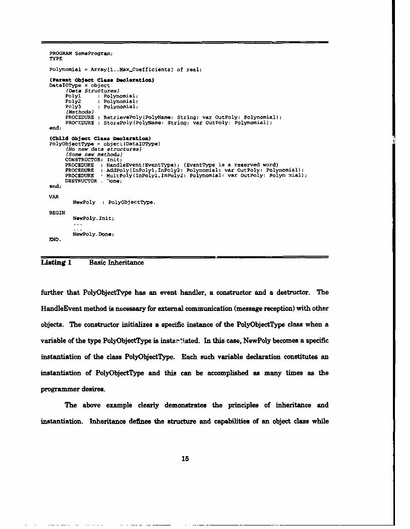
program. For example, an object called NewPoly, an instantiation of class PolyObjectType
which is a child of the parent class DataIOType, could be declared with the statements in
Listing 1.
In this example, a parent object class called DataIOType is defined to have three
polynomials (two operands and a result) and basic file 1/0 procedures to retrieve and store the
polynomials to file. The object class PolyObjectType is declared as a child of DataIOType.
Thus, it inherits all three polynomials and the two 1/0 procedures (methods) from DataIOType.
They are present in PolyObjectType just as though they had been explicitly declared. Note
14
PROGRAM SomeProgram;
TYPE
Polynomial = Array[1..MaxCoefficients] of real;
(Parent Object Class Declaration)DataIOType = object
(Data Structures)Polyl : Polynomial;Poly2 : Polynomial;Poly3 Polynomial;(Methods)
PROCEDURE RetrievePoly(PolyName: String; var OutPoly: Polynomial);PROCEDURE StorePoly(PolyName: String; var OutPoly: Polynomial);
end;
(Child Object Class Declaration)PolyObjectType = objecL(DataIOType)
(No new data structures)(Some new methods)
CONSTRUCTOR: Init;PROCEDURE : HandleEvent(EventType); {EventType is a reserved word)PROCEDURE : AddPoly(InPolylInPoly2: Polynomial: var OutPoly: Polynomial);PROCEDURE MultPoly(InPolyl,InPoly2: Polynomial: var OutPoly: Polyn mial);DESTRUCTOR . )one;
end;
VARNewPoly : PolyObjectType;
BEGINNewPoly. Init;
NewPoly. Done;END.
Listing I Basic Inheritance
further that PolyObjectType has an event handler, a constructor and a destructor. The
HandleEvent method is necessary for external communication (message reception) with other
objects. The constructor initializes a specific instance of the PolyObjectType class when a
variable of the type PolyObjectType is instartiated. In this case, NewPoly becomes a specific
instantiation of the class PolyObjectType. Each such variable declaration constitutes an
instantiation of PolyObjectType and this can be accomplished as many times as the
programmer desires.
The above example clearly demonstrates the principles of inheritance and
instantiation. Inheritance defines the structure and capabilities of an object class while
15
instantiation defines lines of ownership and control of actual data. The two concepts are quite
different and understanding this difference is key to understanding OOP.
Polymorphism: If a child class redefines a method of its parent class, it is said to be
polymorphing that method. For example, if the previous example class PolyObjectType defined
a method called RetrievePolyjust like in its parent, and then changed the program statements
RetreivePoly executes, then one would say PolyObjectType polymorphed the method
RetreivePoly. [Borland, undated:95]
Object-Oriented Analysis (OQA): OOA is an approach to problem definition and
partitioning. OOA initially generates the high level design of objects from which OOD is then
initiated. OOA attempts to identify the classes and objects that model the application context.
Domain analysis attempts to identify the classes, objects, operations and relationships that
are common to all applications within a specified domain. Classification of classes in this
proceas can be quite difficult in general. Approaches to classification include categorization,
clustering and prototyping. Categorization groups entities together based upon properties or
characteristics that form a predefined category. Clustering refers to grouping entities
according to some high level description such as name. Prototyping refers to the predefining
of a prototypical type for a class of objects and other objects are members of that class if they
resemble this type. [Pressman, 1987:146-148]
Object-Oriented Design (QOD): OOD is a design methodology using 00 decomposition
with appropriate icons for 2D presentation. The OOD process consists of identifying the
classes and objects at some level of abstraction, identifying the data and operations of each
class and object, identifying the relationships between classes and objects, and implementing
classes and objects into modules. [Pressman, 1987:334]
Object-Oriented Programming (00P): OOP is a programming technique in which the
data structures are represented as cooperating collections of objects, each object being an
16
instance of a class within a hierarchy of classes that permit inheritance. OOD and OOP
evaluation of objects (or classes) can be done using standard programming discipline metrics
such as object coupling, cohesion, sufficiency, completeness and primitiveness. Coupling refers
to the relationship between objects, cohesion refers to the relationship between internal object
constructs, sufficiency and completeness refer to the object having enough of all possible
behaviors so as to be useful, and primitiveness is when a desired program behavior can only
be implemented by accessing invisible structures of an object. [Pressman, 1987:230-2321
OOD Notation: Notation of OOD can be expressed in a set of hierarchical graphs:
class diagrams, object diagrams, module diagrams, process diagrams, state transition diagrams
and timing diagrams. Although not elucidated here, specific icons are associated with the
characteristics of each diagram. A class diagram presents each class and its relationship with
other classes. The dynamic behavior of the class is represented by a state transition diagram
which portrays the transition from state to state as caused by an event as well as the actions
resulting from a state change. The object diagram presents each object and its relationship
to others. Since objects are created and destroyed during program execution, the object
diagram represents the dynamics of the object. Object diagrams are prototypical
classifications, so it follows that class and object diagram development documents the logical
design of the system. Module diagrams present the encapsulation of classes and objects. All
the diagrams should be evaluated in terms of the formerly mentioned programming metrics.
Furthermore, message synchronization between objects should be defined on these diagrams.
Message synchronization types include simple, synchronous, balking, timeout, and
asynchronous.
2.1.2 The OOD Process. The OOD process consists of identifying the classes
and objects at some level of abstraction, identifying the data and operations of each class and
17
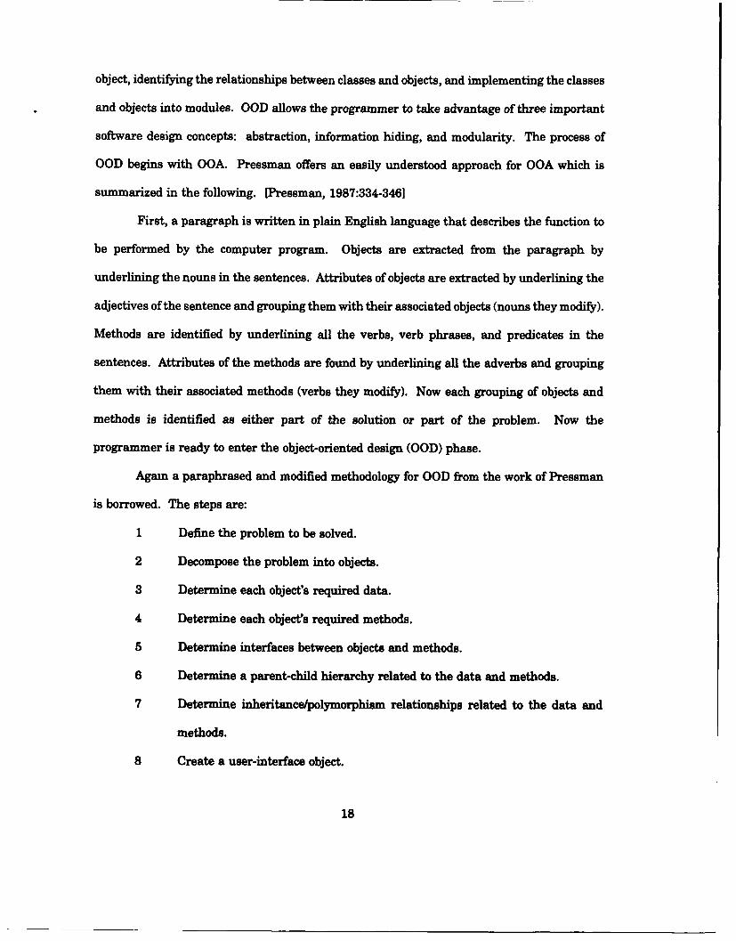
object, identifying the relationships between classes and objects, and implementing the classes
and objects into modules. OOD allows the programmer to take advantage of three important
software design concepts: abstraction, information hiding, and modularity. The process of
OOD begins with OOA. Pressman offers an easily understood approach for OOA which is
summarized in the following. [Pressman, 1987:334-3461
First, a paragraph is written in plain English language that describes the function to
be performed by the computer program. Objects are extracted from the paragraph by
underlining the nouns in the sentences. Attributes of objects are extracted by underlining the
adjectives of the sentence and grouping them with their associated objects (nouns they modify).
Methods are identified by underlining all the verbs, verb phrases, and predicates in the
sentences. Attributes of the methods are found by underlining all the adverbs and grouping
them with their associated methods (verbs they modify). Now each grouping of objects and
methods is identified as either part of the solution or part of the problem. Now the
programmer is ready to enter the object-oriented design (OOD) phase.
Again a paraphrased and modified methodology for OOD from the work of Pressman
is borrowed. The steps are:
1 Define the problem to be solved.
2 Decompose the problem into objects.
3 Determine each object's required data.
4 Determine each objects required methods.
5 Determine interfaces between objects and methods.
6 Determine a parent-child hierarchy related to the data and methods.
7 Determine inheritance/polymorphism relationships related to the data and
methods.
8 Create a user-interface object.
18

9 Create each object.
The first four steps are already arrived at in the OOA phase of the design. Obviously,
there exist many techniques for iteratively applying these four steps further down levels of
abstraction until finally arriving at the primitive level. At this lowest level the objects
required to solve the problem are obvious, as are the methods they need to perform, and the
data they need to own.
Determining interfaces between objects and methods is done by determining how each
object depends on the others. From this it can be determined what mpssages each object needs
to send to the other objects and when. Thus event-handling routines are designed for each
object, so they can perform the desired methods when the message is received.
The next two steps are very much related and display one of the advantages of OOP
at the implementation level. The objects that have methods and data types in common are
grouped into classes. These classes can be completely separate from one another, or they may
have common data items or common methods. Whenever possible, blocks of code should not
be repeated, so the common data and methods are grouped into a class of their own and other
classes are made children of that new class. This class may not make sense as an object in
itself and there may never be an object who is a direct instantiation of it, but its children have
tighter code since they have this library of ready-made methods to use.
Now the step of creating an object who serves as the menuing system and output
screen interface between the human user and the internal objects is added. This object
contains the overall event-handling method as well as most of the Mfie I/O and screen 1/0.
The final step is to pick a particular language and implement the design in code. The
next section describes just such a language.
19
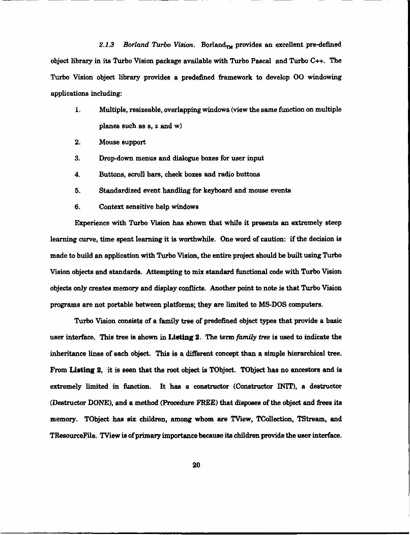
2.1.3 Borland Turbo Vision. BorlandTM provides an excellent pre-defined
object library in its Turbo Vision package available with Turbo Pascal and Turbo C++. The
Turbo Vision object library provides a predefined framework to develop 00 windowing
applications including:
1. Multiple, resizeable, overlapping windows (view the same function on multiple
planes such as s, z and w)
2. Mouse support
3. Drop-down menus and dialogue boxes for user input
4. Buttons, scroll bars, check boxes and radio buttons
5. Standardized event handling for keyboard and mouse events
6. Context sensitive help windows
Experience with Turbo Vision has shown that while it presents an extremely steep
learning curve, time spent learning it is worthwhile. One word of caution: if the decision is
made to build an application with Turbo Vision, the entire project should be built using Turbo
Vision objects and standards. Attempting to mix standard functional code with Turbo Vision
objects only creates memory and display conflicts. Another point to note is that Turbo Vision
programs are not portable between platforms; they are limited to MS-DOS computers.
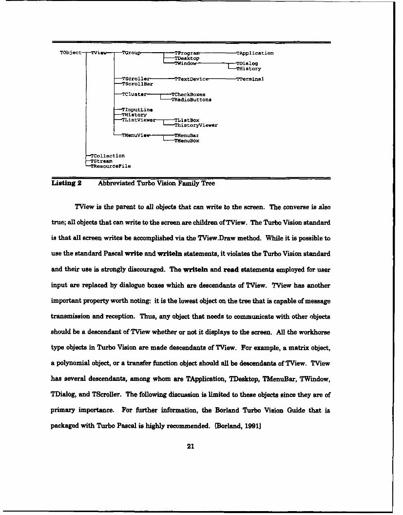
Turbo Vision consists of a family tree of predefined object types that provide a basic
user interface. This tree is shown in Listing 2. The term family tree is used to indicate the
inheritance lines of each object. This is a different concept than a simple hierarchical tree.
From Listing 2, it is seen that the root object is TObject. TObject has no ancestors and is
extremely limited in function. It has a constructor (Constructor INIT), a destructor
(Destructor DONE), and a method (Procedure FREE) that disposes of the object and frees its
memory. TObject has six children, among whom are TView, TCollection, TStream, and
TResourceFile. TView is of primary importance because its children provide the user interface.
20
TObject- -TView-- -TGrou - ITProgra.t TApplication--TDesktopTWndo Dialog
L--Tistory
-- TScroller- TTextDevic-----------TTerminal-- TScrollBar
-- TCluster --- TCheckBoxes---- TRadioButtons
-- TInputLine-- THistory--- TListViewer-----TListBox
--- ThistoryViewer
-- TMenuView--I7-TMenuBar"•----TMenuBox
ollection
Stream-esourceFile
Listing 2 Abbreviated Turbo Vision Family Tree
TView is the parent to all objects that can write to the screen. The converse is also
true; all objects that can write to the screen are children of TView. The Turbo Vision standard
is that all screen writes be accomplished via the TView.Draw method. While it is possible to
use the standard Pascal write and writein statements, it violates the Turbo Vision standard
and their use is strongly discouraged. The writein and read statements employed for user
input are replaced by dialogue boxes which are descendants of TView. TView has another
important property worth noting: it is the lowest object on the tree that is capable of message
transmission and reception. Thus, any object that needs to communicate with other objects
should be a descendant of TView whether or not it displays to the screen. All the workhorse
type objects in Turbo Vision are made descendants of TView. For example, a matrix object,
a polynomial object, or a transfer function object should all be descendants of TView. TView
has several descendants, among whom are TApplication, TDesktop, TMenuBar, TWindow,
TDialog, and TScroller. The following discussion is limited to these objects since they are of
primary importance. For further information, the Borland Turbo Vision Guide that is
packaged with Turbo Pascal is highly recommended. [Borland, 19911
21
Also from Listing 2 it is seen that TApplication is a child of TProgram which is a child
of TGroup which is a child of TView. Thus TApplication is a descendant, several generations
removed, of TView. The focal point of any Turbo Vision program is always a child of
TApplication which the programmer must define. This object owns all other objects through
instantiation, owns the screen desktop, handles all message dispatching, communicates
directly with the main menu, manages idle times, and processes computer errors.
Furthermore, there should only be one TApplication object for any given program, because
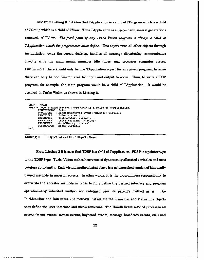
there can only be one desktop area for input and output to occur. Thus, to write a DSP
program, for example, the main program would be a child of TApplication. It would be
declared in Turbo Vision as shown in Listing 3.
PDSP = ^TDSPTDSP = Object(TApplication)(Note TDSP is a child of TApplication)
CONSTRUCTOR: Init;PROCEDURE : HandleEvent(var Event: TEvent); virtual;PROCEDURE : Idle; virtual;PROCEDURE : InitMenuBar; virtual;PROCEDURE : InitStatusLine; virtual;PROCEDURE : OutOfMemory; virtual;DESTRUCTOR : Done; virtual;
end;
Listing 3 Hypothetical DSP Object Class
From Listing 3 it is seen that TDSP is a child of TApplication. PDSP is a pointer type
to the TDSP type. Turbo Vision makes heavy use of dynamically allocated variables and uses
pointers abundantly. Each virtual method listed above is a polymorphed version of identically
named methods in ancestor objects. In other words, it is the programmers responsibility to
overwrite the ancestor methods in order to fully define the desired interface and program
operation--any inherited method not redefined uses its parent's method as is. The
InitMenuBar and InitStatusLine methods instantiate the menu bar and status line objects
that define the user interface and menu structure. The HandleEvent method processes all
events (menu events, mouse events, keyboard events, message broadcast events, etc.) and
22
sends messages to the proper objects in response to these events. The OutOfMemory method
guards against memory overflow errors and the Idle method does background maintenance
during idle periods when the user has not requested any commands.
TDialog is a child of TWindow which is a child of TGroup which is a child of TView.
Descendants of TDialog provide pop-up dialogue boxes for user input. Dialogue boxes contain
radio buttons, check boxes, list boxes, and input lines. Radio buttons are input devices that
allows the user to choose only one item among a list of options. Check boxes are input devices
that allow the user to choose any combination of items among a list of options. List boxes
provide a list of items to choose from such as files on disk or directories. Input lines provide
text entry of string variables. Each of these (radio buttons, check boxes, list boxes and input
lines) are themselves object descendants of TView. Specifically TRadioButtons is the radio
button object, TCheckBoxes is the check box object, TListBox is the list box object and
TInputLine is the input line object. Each are polymorphed and instantiated into a descendant
of a TDialog object by the programmer. Examples are abundant in the Turbo Vision Guide.
[Borland, 19911
Other objects worth brief mention are TDesktop, TMenuBar, TStatusLine, and
TWindow. TDesktop is a child of TGroup which is a child of TView. It is simply the
background view upon which all other visible views appear. TMenuBar is the menu bar object
that displays and controls drop down menus. TStatusLine provides a bottom frame to display
and control shortcut keystrokes and other useful information such as remaining heap size.
TWindow is merely a frame that borders views with a frame.
Event Handling is always a big design concern in OOP. In Turbo Vision, all event
handling is processed via a TEvent type record. TEvent is a record that identifies the type of
event that has occurred and the specific command that has been requested. All events are not
commands; however, all commands are events. For example, the movement of a mouse pointer
23

is not a command, but it is an event. All Turbo Vision objects have event handlers to process
TEvent records; however, the polymorphed descendant of TApplication is the focal point for
all event handling. Assume the basic event handler in Listing 4 is defined for the TDSP
descendant of TApplication described in Listing 3.
PROCEDURE TDSP.HandleEvent(var Event: TEvent);{Note the Event variable is a record of TEvent type)
procedure DosShell;begin
end;
beginTApplication.MandleEvent (Event);if Event.What = evKeyDown then begin
(Desktop Hotkeys)'A', 'a': About;'C', 'c': Calculator;'X', Ix': DosShell;
end;
if Event.What = evConmand then begincase event.comnand of
cmTFCopy Message(TransFunction, evBroadcast, brTFCopy , nil);cmTFDefine : Message(TransFunction, evsroadcast, brTFDefine nil);cmTFDisplay : Message(TransFunction, evBroadcast, brTFDisplay, nil);
end;end;
end;
Listing 4 Event Handler For Hypothetical DSP Object
This example shows the basic operation of a hypothetical TDSP event handler. Note
that the first action taken is a call to the parent's event handler (TApplication.HandleEvent).
This is to process non-command events such as mouse movement and cursor key presses.
Turbo Vision does a nice job of handling these maintenance events and relieves the software
engineer from a great burden! If the Event.What field is equal to the predefined integer
constant named evKeyDown and the key pressed is an a, c, or x, the appropriate subroutines
are called. For proper OOP, these subroutines should be local to the TDSP.HandleEvent
method. If the Event.What field is equal to one of the predefined integer constants named
cmTFCopy, cmTFDefine, or cmTFDisplay, TDSP.HandleEvent sends a message to an object
instantiated as TransFunction. Note that (1) the message is directed to a specific instantiated
24
object and that (2) message transmission is a predefined function of Turbo Vision. Thus the
software engineer is again relieved of a great burden! The message is transmitted as an event
of evBroadCast type and sends the command brTF... which is a predefined integer constant
(the software engineer must predefine these constants in a global unit). The TransFunction
object must then contain its own event handler to receive this message and process it
accordingly.
As demonstrated in the previous paragraph, Turbo Vision provides several tools to
relieve the software engineer of many mundane chores of interface design while allowing all
the benefits of programming in a standard high-level language. Execution speed, numerical
precision, and mathematical algorithms are all designed with far greater control and efficiency
in a fourth generation language (4GL) than could ever be attained by commercial control
system packages designed with their own language interpreters. Once the initial steep
obstacle of learning OOP and the Turbo Vision 4GL are mastered, building applications
becomes a quick and rewarding task.
2.1.4 Advantages of OOP Over Functional Programming. The following
opinions were formed from specific experiences in modifying and debugging the functional
version of ICECAP-PC and then translating it into 00 code. While the experiences discussed
here are from a specific package, they can certainly-based on current literature of similar
design projects--be generalized.
A typical danger spot in functional programming is opening a data file in one section
of the code and then closing the fie in some later section of code. The danger is in forgetting
to close the fie or in bypassing the close command with an unexpected conditional branching
statement. In OOP, a database-type object is used that is the only object in the program that
can get and save data from a particular file. Therefore, for each data file only one open
25
command and one close command are used for the entire program. This abstracts the file I/O
function so that the programmer need only call the database object to read or write to the file
without worrying about opening or closing the file. The drawback to this approach is speed.
If each read from a data file must open and close the file, reading in an entire frequency
response listing will take considerable time. Furthermore, it is easier to store some data files
as sequential files, not as random access files which the data base object approach requires.
Thus, in some situations the data base concept has been abandoned for the traditional
approach; however, strict adherence to a single open and close command per ifie is still
vehemently enforced.
Another drawback in functional programming is the clutter that arises from the user
interface code. Again OOP uses an object to abstract this task from the programmer. The
user interface object abstracts the programmer from having to worry about any user I/O while
writing the mathematical code, etc. One object deals with user requests and translates them
into event messages to be sent to the workhorse objects. Likewise, the same object returns the
workhorse answers to the user in some appropriate screen format.
The same nature of abstraction in OOP allows the software engineer to abstract a
problem to a higher level for debugging or original design. For example, if the programmer
is developing code in the math object and needs to tell the user interface object to print an
answer to screen, he does not need to know how the user interface object does it, he just sends
the user interface object a message telling it what information to print, and the user interface
object can take care of it. From the software engineer's point of view during debugging or
design, he can design at the highest level of abstraction listing the upper level tasks that need
to be done to solve the problem and assume that some object can do each task. Then the
programmer moves down one level of abstraction and takes each task and breaks it down into
sub-tasks assuming some object (or method) can do each sub-task. This is done down to the
26
primitive/coding level. Debugging is broken down the same way. The programmer looks at
the input and output of the highest level object. If it is wrong, he looks at the input and
output of each of the objects in the next level down. He then only has to break down the
object that has incorrect output. Because each object is self-contained, it makes maintenance
very easy.
After the main objects in the program have been fully defined in terms of what data
they need and what methods they need, inheritance is used to decrease the size of the code.
Parent objects are defined for all the main categories of workhorse objects. The parent objects
contain all the methods that the workhorse objects hold in common. This means that each of
the workhorse objects can be smaller because they can globally access the methods they inherit
from their parent. The parent contains methods to decipher user textual input, ones to work
with data files, and other general purpose type methods.
OOP disciplines produce more reliable code due to modular debugging and using
existing objects that have been debugged through years of use. In the case of ICECAP-PC, the
benefits of two worlds have been inherited. At the lowest level, the program has its I/O based
on a commercially produced and tested package (Turbo Vision). At mid-level, the object
methods are based on the basic control system algorithms from ICECAP-PC (developed over
several thesis projects and used by a large student body for many years). After the 00
program had been tested at all levels of abstraction and it was apparent that each object
performed its functions properly and that all the objects communicated among themselves
properly, new objects could be added to the existing reliable code with a high degree of
confidence in the reliability of the CACSD package as a whole.
The same OOP disciplines produce more maintainable code due to the self-sufficiency
of objects. Proper OOP techniques avoid the use of global variables and low functional
independence which often plagues functional program modules. If each object is compiled
27
separately and it responds with expected output responses to test inputs, then it does not
display the undesirable dependence qualities of low cohesion or coupling with some other
object. This research finds that following proper OOP disciplines results in highly cohesive
code, because each object is functionally bound to operate on its data alone. Of course, while
objects higher on the parent-child tree own more data, they still perform only one higher level
function: it receives messages to change its data in some way, and it can do it. Then that
higher level object is made up of smaller objects who are each functionally bound to operate
on their more specific piece of data. This recurses down through the object tree until the
primitive level is reached. At this lowest level, very cohesive methods (subroutines) are
written. In the same way, following proper OOP disciplines results in low coupling between
objects, because each object is again functionally bound to operate on its data alone.
2.1.5 Disadvantages of OOP Gver Functional Programming. Only two
disadvantages with using OOP have been experienced, neither of which are directly related
to OOP itself. The first can be attributed to learning a new programming language and
learning a new way of thinking about algorithms to solve problems. The second can be
attributed to the decision to operate within an MS-DOS environment.
Any time a new programming syntax must be adopted, there is a learning curve that
must be overcome. With OOP this is doubly true, because not only must the syntax of Turbo
Vision, or some other 00 language package, be learned, but the software engineer must also
change their logical concept of problem solution. Humans typically think in functional (data
flow) terms. For example, if a person wants to sign their name on a piece of paper, the
algorithm they might imagine to solve this problem might be:
28
(a) I he'd inkpen.
(b) I lay paper flat on table.
(c) I move inkpen to trace out my name.
The person who thinks in terms of objects might imagine this algorithm:
MAN: Name, sign yourself.
NAME: Paper, display me.
PAPER: Hand, lay me flat on the table.
INKPEN: Hand, use me to trace out the NAME pattern on the PAPER
In this example, consider the HAND as being the primitive level or the coding level
of the methods. Humans tend to think more in terms of the first example scenario; therefore,
the transition into OOP is not as intuitively easy as using functional programming techniques.
Any time code is developed within the MS-DOS environment, limitations are placed
on how much memory room is available for use by the program. A stack cannot be larger than
64K, variable declarations cannot be larger than 64K, and the compiled program and heap
space (dynamic variable space) cannot exceed 640K. The 640K barrier can be overcome in
Turbo Pascal by breaking the compiled code into overlay units, but even then each overlay unit
cannot be larger than 64K and must be able to be compiled to some extent separately from the
other units. These memory restrictions place some limit on how closely a programmer can
follow the generally accepted rules of OOP.
2.1.6 Summary of OOD and OOP. Object-oriented design and programming
have grown to a standard practice because of benefits over functional design and
programming. Such advantages include the reuse of existing software components, more
maintainable systems, reduction of developmental risk, and use of OOP language constructs.
Disadvantages include the higher cost of development and possible performance degradation
29
due to message passing, the multi-layer abstraction, hierarchy of classes, and associated
memory and execution overhead.
The 00 approach generally results in smaller systems because of reusable subsystems
and thus are more amenable, providing a economic framework for evolution. The original
ICECAP-PC was developed using the functional design approach as were its predecessors. The
new 00 version of ICECAP-PC provides for better maintenance and user interface.
2.2 Literature Review of Human Interface Design
The quality of a computer package's user-interface is important to the user as well as
to the software developer, because if the user does not like to use the software, it may become
what the industry calls shelfware and never be used. It is a common trap for a software
developer to take the attitude that his software is so powerful that the customer would be
crazy to not want to use it. But while professional salesmen can make any good package look
amazingly powerful during the in-store demonstration, it is the great package that can be
brought back to the office and allow the practicing engineers to make it look amazingly
powerful. The difference between these good and great packages is the user-interface.
Desiring ICECAP-PC to be a great CACSD package, the goal of this thesis effort is to design
a user-interface which engineers feel comfortable using.
AFIT thesis students have been developing ICECAP-PC since 1984, and it has gained
a large user base that spans the US. It is a living package in that user response forms are
constantly received and used to improve the software. The user response forms typically cover
three main topics: can a new capability be added to ICECAP-PC, can an existing capability
be corrected, and can an interface function be corrected/modified. A vast majority of the
response forms and complaints from local users deal with the last topic: user-interface. Many
students have at times become frustrated with the ICECAP-PC interface as they spend
30

valuable homework time traversing the hierarchical menu structure trying to get the package
to produce the desired results. Even though advanced users can type in complete strings of
commands at one time, access to the underlying commands are still not very easily accessed.
This is why it is important for AFIT thesis work to focus on improving the ICECAP-PC
user-interface. Furthermore, providing AFIT students and government engineers with a free
CACSD package fills a potentially expensive need for the US Government. Software licenses
for commercial packages with no more capability than ICECAP-PC can cost $1000 per user.
Thus, ICECAP-PC fills a viable need by remaining a state-of-the-art CACSD package. With
new object-oriented technology and advanced menuing techniques along with HFE principles,
ICECAP-PC can once again challenge the state-of-the-art in user-interfaces.
The first part of this section describes the current ICECAP-PC user-interface. The
second part describes the technical implications of HFE rules to user-interface design. The
third part describes the user-interfaces of current commercial packages. The combination of
the information described in these sections then produces new design criteria for the improved
ICECAP-PC user-interface.
2.2.1 ICECAP-PC 9.0. ICECAP-PC 9.0 has a user-interface that was
cutting-edge for its time (mid-80s), but the new graphical user-interfaces of today's commercial
software have significantly increased the expectations of today's computer user. The
user-interface for ICECAP-PC 9.0 requires typing in command words, offers no
mouse-activated menus, offers no hot keys (press one function key or CONTROLIALT key
sequence to represent a long command string), offers very rudimentary semi-context-sensitive
on-line help, and offers no interactive graphics displays for plots and graphs.
When the user runs ICECAP-PC, they are presented with a listing of the highest level
command words--one of which is HELP. HELP can be requested fr x basic system use or for
31
specific commands [Moore, 1984:Ch III, 24]. Typing in the word HELP gives pseudo context
sensitive help information. At the highest menu level, help can be requested for the overall
system instead of a menu item. Help is not available at the dialogue screen levels.
The command listing is in the form of four columns sorted alphabetically across the
screen and displayed above a command prompt. The menu command words for different menu
levels are grouped sometimes functionally and sometimes logically (Display, Define, Transform
but then DSP, QFT). The user types in one of the command words (abbreviations are allowed)
at the prompt and is then either presented with a lower level listing of command words or a
question-and-answer dialogue screen in which to enter ranges and other parameters required
to properly display the requested information. An example of a lower level menu might be if
the user types in the command DEFINE at the highest menu level, the next menu level might
list MATRIX, POLYNOMIAL, or TRANSFER FUNCTION in order to specify what is to be
DEFINED. These lower level menus extend four levels deep at the lowest level, before
dialogue screens are finally reached. Two levels deep is the average. Advanced users can
avoid reading all the menu listings by typing in a whole sequence of command words at once.
For example, if an expert user desired a root locus plot, they could type DISPLAY LOCUS TF2
AUTOMATIC, instead of typing each command separately and waiting for a new menu listing
before typing in the next command word. [Moore, 1984:Ch II, 131
After the user has specified the information they desire to see by entering up to four
levels of command words, they then must answer question dialogue screens up to four screens
deep. Dialogue screens request the user's desired axis ranges, data format, plot titles, forcing
functions, etc. Once the graph or listing is displayed on screen, the user has no way to
interact with it. They cannot change the scale or change some model parameter to see how
it affects the graph. Their only recourse is to press the ENTER key and be sent all the way
32
back to the highest menu again where they type in the same command words and reanswer
the dialogue screens.
Another symptom of an aging user interface is the uninformative error messages
ICECAP 9.0 generates for the user. If the user types in a number wrong-- if they accidentally
enter a letter--or if they enter an unrecognized command, the program responds with the
message "input not a number" or "invalid command," and returns the user to the blank prompt
to reenter the text. It gets worse when an error in the program causes the whole system to
crash, because then all the user is given is a cryptic Turbo Pascal error number and the
hexadecimal memory location where it occurred, and the program exits unceremoniously to the
DOS prompt. All the user can do then is restart the program and begin again.
A third shortcoming of the interface system is that some program commands assume
other commands have been previously performed. For example, for no apparent reason to the
new user, ICECAP-PC does not display a requested graph. No error message is given; just
the wrong graph or an empty graph is displayed. The more experienced user has learned that
sometimes hidden sequences of commands must be entered before certain operations perform
as desired. To display a root locus of OLTF, it is assumed that OLTF has already been
defined. Transforming from the S to the Z domain assumes that the sampling period has
already been set under the MODIFY command. Even worse, MultiPlots assume you have
already saved the data files using the UPDATE command. To display a graph of a frequency
response assumes you have already displayed a listing of the frequency response. This type
of pseudo-error grows more common as the user enters the more advanced toolboxes within
ICECAP-PC, like the digital signal processing or the root locus sections.
There are some further annoyances with the graphic routines within ICECAP-PC.
First, the dialogue screens for graphics have only a few options per screen so the user is
brought through several screens before they see any graphs. Second, the many dialogue
33
screens do not offer default values for their data fields, and the data must be entered every
time because the fields have no memory of what they were the last time. Third, when a
frequency response listing for a certain range of frequencies is generated, the graph can be
displayed for different ranges of frequencies, but the data file is not regenerated. This means
that while the limits of the graph has changed, the resolution of the data has not changed.
And the final annoyance is that all graphics displays are non-interactive. Even to just change
the range of frequencies displayed on the graph, the user must exit from the graph all the way
back to the very top menu and reenter every command and every dialogue screen to redisplay
the graph with new limits. And if they want that better resolution, they must first go through
all the commands to regenerate the listing of the response data.
In summary, ICECAP-PC offers the functions required to do CACSD, but it lacks the
polish today's user expects from a software package. However, while the user must type in
command words through several layers of menus to finally get to the data display, at least all
their options are always displayed for them at every prompt. So while it is cumbersome to
use, users do eventually figure out how to get the results they desire.
2.2.2 Human Factors Engineering. It has not been until the last few years
that HFE has become an essential part of software design. It has not been that software
designers consider HFE unimportant, they just could not accommodate the added overhead
HFE techniques required. The limitations of computer resources in processing power, graphics
resolution, and memory size limited software designers to worrying only about accomplishing
tasks; limited resources were available for worrying about how a task was accomplished. But
in the last five years, personal computers have exploded the amount of resources available to
software designers. The Intel 486 processor and Super VGA graphics and four-megabyte
memory chips allow plenty of resources to not only accomplish a task but also offer enough
34
power to handle the overhead of an elaborate graphical user-interface system. So now that
the computer industry can accommodate the demands of the HFE community, HFE specialists
have a voice in the design of new software systems. The following paragraphs discuss some
of these current voices.
2.2.2.1 Ravn. Ole Ravn made an insightful summarization of
the HFE shortcomings of most CACSD package user-interfaces. He said that most CACSD
packages today "do not support the user in the iteration process of solving a design problem."
He explains that these packages are just a collection of toolboxes into which the user can put
an input and get some output, but that "the combination of these tools are [sic] up to the user.
... It is up to the user to evaluate the results and decide what to do next." He also explains
that most packages do not offer user interaction with the displayed data allowing the user to
change some parameter and see how it affects the displayed graph (or whatever). He closes
by pointing to the inability of most packages to allow the user to interact in one domain
(frequency, time, etc.) and watch the effects on a display in another domain. His work in
designing user-interfaces shows the best method is to allow the user to communicate their
desired command by selecting labeled buttons on graphics screens using a mouse. The
resulting information display remains on the same screen as the command buttons allowing
it to be iteratively changed by adjusting model parameters, etc. The user is able to modify
what command buttons appear on the screen and even to modify what they do when selected.
Multiple views of the same information can be put on the screen at the same time thereby
allowing changes made in one domain to be displayed in other domains or graph types. Each
view is updated once the user changes the parameters in any of the other views. Context
sensitive help is available on any object or command on the screen just by pointing to it with
the mouse and pressing a mouse button. [Ravn, 1989: 35-38]
35

2.2.2.2 Barker. H. A. Barker and several other British
engineers from the University College of Swansea also grilled the state-of-the-art command
line driven CACSD packages and called for mouse-driven, interactive graphical user-interfaces.
These authors also describe mouse-selectable labeled buttons and warn against hierarchical
menus which can have many levels of depth and slow down the user. These authors also point
out five important advantages of graphical user-interfaces to the engineering user. First,
novice users find graphical interfaces easier to learn and more like the way they might solve
the problem with pencil and paper. Second, the graphical interface may allow new design
techniques by grouping large amounts of input information into a single icon or by displaying
information in ways never before practical. Third, multiple windows allow the engineer to see
how data changed in the design window directly affects the data presented in the simulation
window. Or perhaps the engineer might display three different simulation windows to see how
his changes affect different experiments. Fourth, pictures of everyday items can make the
data presentation seem more intuitive to the user and remove a layer of haze from the design
process. Finally, if all CACSD packages use a standard graphical representation of data, new
packages or new additions to packages will be easier to learn. [Barker, 1989:881
2.2.2.3 Smith. Sidney L. Smith has been publishing guidance
on applying HFE to software for over 30 years. His document to be summarized herein
contains over 944 HFE guidelines for designing software user-interfaces, and is probably the
most complete and practical work in the field. The guidelines cover the areas of data entry,
data display, data transmission, data protection, sequence control, and user guidance. While
122 of his guidelines directly apply to the new ICECAP-PC user-interface, listing and
discussing each of them is beyond the scope of this paper. However, some of his more general
statements are listed here. It is also important to note that the two areas of data transmission
36

and data protection are not discussed at all, because they are not needed for the ICECAP-PC
user-interface.
First, Smith presents the general objectives of good data entry design. "The general
objectives of designing data entry functions are to establish consistency of data entry
transactions, minimize input actions and memory load on the user, ensure compatibility of
data entry with data display, and provide flexibility of user control of data entry." He goes on
to give hundreds of specific rules for keystrokes, text editing, forms and tables, plots and
drawings, and default values. [Smith, 1986:111
Second, Smith presents the general concepts for data display. He says context,
consistency, and flexibility are the most important concepts. "Somehow a means must be
found to provide and maintain context in data displays so that the user can find needed
information.... Design guidelines must emphasize the value of displaying no more data than
the user needs, and the importance of maintaining consistent display formats so that the user
always knows where to look for different kinds of information, on any one display and from
one display to another." He again goes on to give hundreds of specific rules for text and
graphic displays, forms and tables, data ordering and spacing, colors, and windowing
techniques. [Smith, 1986:931
Third, Smith presents the general guidelines for sequence control. He explains that
while both consistency of control actions and minimal control actions required of the user are
both important, consistency must always win in a trade-off. This is because while the designer
might think he is helping the user by reducing required keystrokes by designing some clever
key sequence, the user will probably end up resenting the additional learning and confusion.
The clever key sequences can be included for expert users, but should be invisible to the novice
who wants to see every action executed the same way. This novice-expert flexibility should
be present throughout the user-interface. It guarantees a minimal memory load on the user.
37
He goes on to say that an alternative to special hot keys (this term refers to any keyboard key
combinations that are pressed simultaneously) would be to have command icons displayed on
the screen and allow their activation by a pointing device. He warns against long,
multileveled menus activated by a mouse. The last general guideline for sequence control is
to make the most frequently accomplished tasks the easiest to transact. [Smith, 1986:213-215]
The final topic Smith presents concerns user guidance. "The fundamental objectives
of user guidance are to promote efficient system use (i.e., quick and accurate use of full
capabilities), with minimal memory load on the user and hence minimal time required to learn
system use, and with flexibility for supporting users of different skill levels." Smith presents
scores of rules dealing with error messages, alarms, prompts, labels, and documentation. He
proclaims the need for context sensitive help down to the command or error message level.
He also says that the help system should allow general browsing through its contents allowing
the user to read all available help on every topic. [Smith, 1986:291, 330-331]
2.2.3 Commercial Packages. This section analyzes each commercial package
against three criteria. First, the menuing system must be efficient and intuitive. It must be
flexible enough to teach and guide the novice without hindering the expert from quickly
accessing the power of the underlying routines. It must not add considerable time overhead
which significantly increases the time required to solve the problem at hand. Second, the
on-line help must provide guidance at appropriate levels. Third, the presentation of
information on the computer screen must enhance the utility of the system. For example, the
color or the way information is displayed must not be distracting or awkward to the engineer.
And if the displayed information does not look the same as it would if the engineer were
working the problem on paper, the differences must add some new insight into the data and
not just be arbitrarily chosen to be different. Also, the user should be able to interact with the
38
graphics display in order to modify parameters and watch the effects these changes have on
the graphics display. These systems are not being ranked or graded, rather, their best aspects
are mimicked and their worst aspects are avoided.
2.2.3.1 MicroSoft Windows
2.2.3.1.1 Menuing System [Microsoft, 1990:251. In the
last year, Microsoft Windows 3.0 has quickly become the standard menuing system for both
business and entertainment software. While this is probably due more to Microsoft's
dominance of the software industry than to their application of HFE to Windows' graphical
user-interface, any user-interface designer should weigh the advantages of emulating the
Windows menuing system. New users of their system would learn the interface quickly since
it looks and feels like their other Windows software. Microsoft has certainly invested immense
assets into HFE studies on how to design a good user-interface, so by emulating their results,
the new design would probably inherit the benefits of their research. And finally, there are
many software development tools available on the market to provide this Windows emulation.
The Windows menuing system is a list of commands displayed across the top line of
the screen. Two specific commands always found are FILE (used for disk access) and HELP
(used for guidance). The novice user selects the desired command by pointing at the desired
command word with the mouse pointer and pressing the mouse button. This produces a
pop-down menu that extends a new list of command words below the command just selected.
The user then selects a command word from that list using the mouse. This command either
produces the desired output or displays a dialogue box prompting for further details before
producing the desired output. The slightly more advanced user can trace through the menu
system without using the mouse by holding down the ALT key and typing the activation letter
39
(activation letters are the underlined letter in a command word display) of the command they
desire. The expert user can also just type a hot key combination corresponding to the
command they desire. A hot key combination can be any combination of the ALT, SHIFT,
CONTROL, alphanumerics, or function keys.
Windows also offers a menuing system enhancement which Microsoft calls a toolbar.
This toolbar is a few rows of icons on the lines right below the menu line. These toolbars are
user-definable to represent any command found in the menuing system. Thus, they offer a
type of mouse-sensitive hot keys. Some of these icons have pop-down menus built into them
that are activated when the icon is selected. These pop-down menus do not contain command
words, instead they contain the options available for whatever the icon represents. For
example, if the icon were the FONT icon and it were selected, its menu would display all the
available fonts for the text, and when the user then selected one, it would become the current
font.
2.2.3.1.2 On-Line Help [Microsoft, 1990:70]. Microsoft
has developed a very elaborate help system for Windows. Help is available either by selecting
the help command word from the main menu or by pressing the first function key (Fl). If the
user selects the menu command word, a pop-down menu is presented offering the opportunity
to browse all on-line help topics. If the user presses F1, context-sensitive help is provided for
whatever command they were currently executing. The help appears in a separate window
with its own menu line and toolbar. The user can open help volumes for any installed
Windows applications, they can search for the occurrence of a specific word or topic in the
current help volume, and they can do other functions related to reading the help files.
2.2.3.2 Directory Commander (dCOM)
2.2.3.2.1 Menuing System [DAC, undated:25-301. The
40
dCOM program is a DOS shell. A DOS shell is simply a user-interface for DOS--DOS, by the
way, stands for Disk Operating System and is simply the command structure that controls the
lowest level computer functions, like looking at the contents of disks and copying disk files.
dCOM is a perfect example of a program whose menu system allows access to any command
by a single hot key combination. When the user presses a hot key, the command is executed
and the results are immediately displayed on the screen. For example, if the screen contains
a listing of all the files on a disk, and the user presses the hot key ALT-T (hold the ALT key
down and press T at the same time), a tag marker appears next to every filename. Then if the
user presses the hot key D, all the tagged files are Deleted. While there are thousands of DOS
shell programs on the market, none are more efficient in their menuing system as dCOM.
dCOM is more efficient than Windows because every possible command has its own hot key,
whereas in Windows less than a quarter of the commands have been assigned hot keys.
2.2.3.2.2 On-Line Help [DAC, undated:44]. VAl*i ft
dCOM menuing system is extremely powerful for the experienced user, it has a very high
learning curve for the new user. There are no command prompts or menu lists asking the user
what to do next, and the on-line help is neither context-sensitive nor very extensive. Pressing
H brings up the only available help. This help is basically just a listing of all the hot keys and
the DOS commands to which they correspond.
2.2.3.3 Turbo Vision
2.2.3.3.1 Menuing System [Borland,1990:7-221. Turbo
Vision is a command library for the programming language Turbo Pascal. Applications written
in Turbo Pascal can use the user-interface support offered by the Turbo Vision package. Turbo
Vision offers the best features of dCOM and Windows as discussed above. It allows either the
mouse or the keyboard to drive the hierarchical menu system and dialogue boxes of Windows.
41
It allows the bypassing of the menu levels by use of a toolbar or hot keys. And it allows, at
the expense of programmer effort, each command to be assigned a hot key as with the dCOM
interface.
2.2.3.3.2 On-Line Help [Borland, 1990:1301. Turbo Vision
allows help messages to be context sensitive down to the current view, where a view is the
current command in a menu listing or the current dialogue box or the current display window.
So the user can use the mouse to select an object they want help on and press the help hot
key, or they can select the help command word from the menu and browse through the help
files. As with Windows, all help appears in a separate window. Commands offered in the help
window include commands to display a table of contents of all help topics and an alphabetical
index of words in the help file. All the functions offered by the Microsoft Windows help system
are available with Turbo Vision, but the displays look different (presumably to avoid a
lawsuit).
2.2.4 CACSD Packages. This study evaluated numerous commercial CACSD
packages. Their menuing systems and help systems were all simple variants of those already
described and are not discussed here. However, these packages offer new information in
determining design rules for the data display portion of a CACSD package user-interface. The
analysis of these packages investigates how they use the display of information to give
engineers new insights into the problems they are trying to solve, and also how they provide
the user with some way to interact with the graphics display in order to see directly the effects
of changing parameters on the graphics display. The packages evaluated are Program CC,
Mathcad for Windows, MatrixX, and Matlab.
42
2.2.4.1 Program CC [Thompson, 1985:Ch 2, 21-261. Program CC is
perhaps the commercial CACSD package most similar to ICECAP-PC. It offers comparable
functions and menuing system and on-line help; however, its data display is slightly superior
in the way it allows user interaction. After a graph is drawn, a menu of display format
commands is also presented. With this menu, the user can change limits of axes, move a
cursor that reports useful screen location data, change foreground and background options,
print the screen, add labels, thicken lines, center the plot, zoom in and out, change the state
output being displayed, add more points in a given range, and compute some figure of merit
values. While allowing the user to interact with the format of the data display is an
improvement over the norm, it still does not allow the user to change the model parameters
and see how this affects the graph. However, Program CC does demonstrate all the necessary
ingredients needed for user-interactive graphics design.
2.2.4.2 Mathcad for Windows [MathSoft, 1991: 13-381. While Mathcad
for Windows is not a CACSD package, it is a complex-math package; therefore, its data display
characteristics are fully transferable to a CACSD package user-interface. The feature that
makes Mathcad unique among all the other packages analyzed is that its input and output
format looks exactly as it would if the user wrote it on paper (in terms of symbol placement,
not in terms of freehand drawing). Answers and graphs are presented just as they would look
on paper drawn manually. Output graphs are generated in resizable regions right on the same
screen as the equations that generated them. And if the user changes any of the equations
affecting the graph (by clicking on them with the mouse and retyping some of the parameters)
the graph is instantly updated. Mathcad is certainly a good demonstration of the technology
desperately needed in today's CACSD packages.
43
2.2.4.3 Matrixx and System-Build. Matrixx is available for
personal computers (PCs) as well as for Sun workstations. The PC version offers no new
information to this investigation, but the Sun version presents a third method for allowing the
user to interact with the graphics display. The basic user-interface is a command line where
the user types in long, complicated command sentences. When the user types in the command
to generate a graph, a graphics window appears at the top right comer of the screen and the
plot is generated. The user can continue typing commands at the command line screen and
add plots to the graph, change the format of the graph, etc. However, the user still cannot
change model parameters and see the changes reflected in the graph. They can change the
model parameters and then request a new graph of these changes to be drawn on the same
graph as the old plot. This is very close to the desired, but still is not very easy to use.
[Integrated Systems, 1986a]
SystemBuild is an add-on package to Matrixx, specifically it is an "interactive,
menu-driven graphical environment for building, modifying, and editing computer simulation
models." Matrixx's SystemBuild package is the best system building interface in the industry.
The user connects icons with input/output lines and defines the icons to represent formulas
and functions. While SystemBuild is clearly part of the data input system, it is mentioned
here in the discussion of data output because if SystemBuild could be paired with the
interactive graphics displays of MatrixX, i.e., if the changes the user made to the graphical
representation of the system model-SystemBuild--could be automatically represented in the
graphics display, a superior user-interface would be the result. This interface would offer the
desired interactive ability and still be very easy to use. [Integrated Systems, 1986b]
2.2.4.4 Matlab [Moler, 1987J. While Matlab is by far the
industry standard for CACSD packages in terms of performance, it is one of the worst for
44
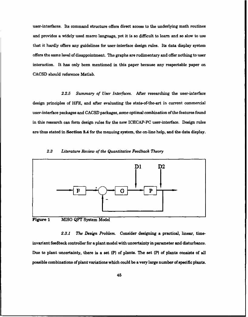
user-interfaces. Its command structure offers direct access to the underlying math routines
and provides a widely used macro language, yet it is so difficult to learn and so slow to use
that it hardly offers any guidelines for user-interface design rules. Its data display system
offers the same level of disappointment. The graphs are rudimentary and offer nothing to user
interaction. It has only been mentioned in this paper because any respectable paper on
CACSD should reference Matlab.
2.2.5 Summary of User Interfaces. After researching the user-interface
design principles of HFE, and after evaluating the state-of-the-art in current commercial
user-interface packages and CACSD packages, some optimal combination of the features found
in this research can form design rules for the new ICECAP-PC user-interface. Design rules
are thus stated in Section 3.4 for the menuing system, the on-line help, and the data display.
2.3 Literature Review of the Quantitative Feedback Theory
D1 D2
Figure 1 MISO QFT System Model
2.3.1 The Design Problem. Consider designing a practical, linear, time-
invariant feedback controller for a plant model with uncertainty in parameter and disturbance.
Due to plant uncertainty, there is a set (P) of plants. The set (P) of plants consists of all
possible combinations of plant variations which could be a very large number of specific plants.
45
The QFT method, developed by Dr Isaac Horowitz, quantitatively defines the problem in the
form of (1) sets {TR) of acceptable command or tracking input/output relations and (2) sets {TD}
of acceptable disturbance input/output relations and (3) a set {P) of possible plants. The design
objective is to guarantee that the control ratio, TR = Y/R, is a member of {TR} for all P in (P).
2.3.2 The Design Approach. The QFT design (QFD) approach is a frequency
domain technique that provides robust performance despite plant uncertainties and
disturbances. The general model has three inputs: a tracking input R, a plant input
disturbance D1 and a disturbance D2 (this can be sensor noise, wind gusts, etc) as shown in
Figure 1. P is the symbol for the plant, G is the compensator to be designed and F is a pre-
filter that also requires design. L = GP is defined as the loop transmission (open-loop transfer
function). If only G is available as a design parameter, the system is referred to as a single
degree of freedom control loop. If F is added, two degrees of freedom are available. Thus, the
QFT method is a two degree of freedom design. This approach has sufficient generality for
modelling a variety of systems.
2.3.3 The Design Procedure. The ICECAP-PC QFT package closely follows
the design procedure specified by Dr Horowitz and Dr Houpis [ID'Azzo, 1988:728). This
procedure is summarized as follows:
1. Synthesize upper and lower tracking response transfer functions TRu
and TRL to meet minimum and maximum specifications.
2. Synthesize TD, the upper disturbance response transfer function.
46

3. Define a set of plants {Pj) from all possible (P) such that the frequency
response of the set (P,) defines the perimeter of all possible frequency
responses of (P).
4. Select a representative nominal plant P. from the set {P(}. Normally,
the best selection is the lower-left plant as seen on a Nichols chart
template.
5. Determine the disturbance bounds BD on the loop transmission L0.
6. Determine the tracking bound BR.
7. Define the composite bounds as the most restrictive combination of the
bounds determined in steps 6 and 7.
8 Design the loop transmission Lo for the nominal plant Po to meet, as
closely as possible, the composite bounds determined in step 7.
9. Synthesize the prefilter F.
10. Simulate system behavior to verify correct design.
2.3.4 Summary of QFT. A detailed discussion of the MISO QFT method and
literature search can be found in the QFT Toolbox User's Manual in Appendix E and is not
repeated here for the sake of brevity.
2.4 Summary
In this chapter, we developed a general basis of knowledge in three critical areas.
First, we discussed the general concepts of object-oriented programming including the analysis,
design, and implementation of 00 program structures. We discussed 00 terminology, talked
about Borland's Turbo Vision 00 fourth generation language, and discussed the advantages
and disadvantages of object-orientation. We found that from the standpoint of software
47
engineering goals, reusability, extendibility, etc, object-orientation is far superior to any other
known construct. However, it does present a steep learning curve as it requires both a
different logic structure and a different implementation structure, presenting the new
programmer with unknowns in both the problem space and the implementation space of a
computer program.
The second general area of discussion was user interfaces. We discovered that there
are many design decisions to be made with the user interface due to the many different ways
of presenting information to the user. We examined the HFE guidelines developed from
scientific research as well as the field-tested interfaces of popular commercial software
packages.
Finally, we developed the general mathematical background for the Quantitative
Feedback Theory. This development provides a roadmap for future implementation of QFT
toolboxes (a complete discussion on the toolbox concept is given in Chapter 4).
The general knowledge attained from the research outlined in this chapter forms the
basis for the specifications given in Chapter 3 and for the actual implementation of ICECAP-
PC as given in Chapters 4 and 5. The next task is to develop the specifications for ICECAP-
PC.
48
3 Requirements and Specifications
This chapter defines the specific requirements of the ICECAP-PC program. First, we
consider general traits such as accessibility, portability, etc. While many of these traits seem
obvious, they do bear on the final platform selection and program structure. Second, we
describe the desired human interface. Third, we develop a list of desired mathematical
capabilities that define the basic math engine of ICECAP-PC.
We do not develop an OOA model as described in Chapter 2. While a complete OOA
model would certainly be expected in large government software contracts, experience dictates
that future ICECAP-PC programmers are unlikely to use it. Little use was found for previous
functional models; therefore, they are deemed an unnecessary expenditure of valuable
development time for this thesis effort. Furthermore, most of the work in developing a highly
complex object structure was accomplished by Borland in developing the Turbo Vision 4GL
which ICECAP-PC inherited in its entirety. The only additional work done in the ICECAP-PC
object structure was to extend the structure with the new ICECAP-PC objects. Therefore, only
a basic object model of ICECAP-PC is given within [Trevino, 19921, and specific object
descriptions are expanded in Chapter 4 as needed to aid in the discussion of the actual
ICECAP-PC structure. By being able to avoid a full OOA of ICECAP-PC and apply a more
prototypical approach to the code design, we are able to produce the broad capabilities of a
CACSD package in the short period of time of a thesis effort. Programmers who desire to work
with the ICECAP-PC code will gain all the insight required by reading this thesis and
[Trevino, 19921. Appendix D, ICECAP-PC Programmer's Manual, provides all the specifics
required to make calls to the ICECAP-PC object methods, while the 00 PASCAL code itself
provides self-documentation.
49
3.1 General Traits
3.1.1 Accuracy. As discussed in Section 1.3.2, numerical accuracy is
fundamental in any CACSD program. We want to provide the best possible numerical support
for control engineering calculations. This has several implications. First, we must insure that
we are using state-of-the-art numerical techniques. To insure this, every major algorithm
must undergo thorough review with outdated procedures being rewritten. Second, because
ICECAP-PC specifically addresses control systems engineering, we can make certain
assumptions. For instance, we can assume that a realizable transfer function has real
coefficients in both numerator and denominator. This directly bears on our root finder as we
can implement a faster and more accurate algorithm by assuming exact conjugates for complex
pairs. Also, we can assume a set range of expected values. Very few control systems--and
certainly no educational control systems--have transfer functions with coefficients less than
1 x 10⁶ or greater than 1 x 10⁸. Thus, the range of numbers where we desire the greatest
accuracy is quite achievable and reasonably defined. Third, the accuracy requirement
encourages the use of the highest precision floating point number supported by standard
software, the IEEE Std 754 80-bit extended real number, for all calculations as discussed in
[Trevino, 1992; IEEE, 19851.
3.1.2 Speed. We desire ICECAP-PC to be very fast in interface and
calculation. First, we seek a nimble, responsive interface that provides rapid command access
and execution. This requires (1) concise interface code, (2) the intelligent use of memory (a
scarce resource in MS-DOS), and (3) an interface based on the fewest possible keystrokes for
command execution. Command line interfaces provide rapid access to commands and direct
control over command options but may be frustrating to an expert control engineer who is not
completely familiar with the package. Menu based interfaces are often sluggish and present
50
too much overhead. We need to combine the best of both worlds providing rapid menus and
single line data (matrix, polynomial, transfer function) definitions. Second we seek rapid
numerical solution wherever possible without risking accuracy.
3.1.3 Reusability. ICECAP-PC is a two-way educational program. First it
provides educational support for the control systems student--the user. Second, it provides an
educational experience for contributing authors who over the years have developed the
program. ICECAP-PC code should be structured in such a way as to provide support to other
engineering students in programming projects. For instance, the mathematical engine should
be easily ported to other programs in other disciplines. This is a matter of code design and
placement.
3.1.4 Portability. ICECAP-PC need not be portable across different platforms
because of the prevailing accessibility of MS-DOS machines on which ICECAP-PC was meant
to run. However, ICECAP-PC should run independently and not require the purchase of
additional software or hardware other than a 80286 or better personal computer. Because of
the numerical sophistication required by ICECAP-PC algorithms, we decided not to support
micro-processors lower than the 80286.
MS-DOS compatible computers come in a variety of configurations, and where possible
we should support advanced features such as expanded memory, math co-processors, high
resolution graphics, etc. Many high level languages specifically address these features as
compiler options and our choice of platform includes these considerations. Indeed, personal
computers based on the 80386 and 80486 family of processors offer considerable improvements
in performance in math operations as well as memory availability.
51

3.1.5 Accessibility. ICECAP-PC should be readily available to the widest
audience possible. Ideally, ICECAP-PC should be available to every controls engineering
student across the country. The best way of achieving this is to write the program for the MS-
DOS compatible platforms as this is by far the most popular computer platform available.
Additionally, the ICECAP-PC program must be an .EXE file, rather than a macro of some
other mathematical program. This keeps a potential user from needing to purchase an
expensive commercial package to host the macro files. In order to make the program
accessible, we also need to provide it at a minimal expense. As ICECAP-PC is a public domain
program, we provide it free of charge to any interested party.
3.1.6 Graphics Presentation. Graphical representation of system responses
is basic to the study of control systems. ICECAP-PC has always provided a rich set of
graphical tools that are easy to use and understand. However, we desire to improve the
graphics engine by (1) providing direct plots of graphic screens to printers, (2) providing
interactive graphics for educational purposes, and (3) providing multiple graphics windows.
Interactive graphics allow the user to modify a transfer function and watch the effect on a
frequency or time response. Thus the user can see directly the effect of added poles and zeros
on a transfer function. This is especially important for the QFT problem. Multiple graphics
windows would allow the display of several graphs at once. For instance, the user should be
able to view both a time and frequency domain plot of a transfer function simultaneously.
Each of these would greatly improve ICECAP-PC. However, we must emphasize that this is
a relatively low priority in this project being superseded by the structural redesign of the
program itself.
52
3.1.7 Intuitive Interface. In Section 1.8.1, we stated that a msjor design goal
was the development of a truly intuitive user interface. Now, based on the research done in
Section 2.2, we list the general characteristics of this interface.
1. The interface should be based on a pull-down menu structure
accessible via keyboard or mouse for ease of use.
2. Keyboard commands should be executed with minimal keystrokes. The
ideal number of keystrokes for a given command execution is 1.
3. The interface should be event-driven. An event driven interface is one
that provides the user maximum control rather than constraining user
actions through a hierarchical menu structure.
4. The interface should be very fast and responsive. Command access
speed should be limited only by the user.
5. The interface should display efficient use of memory and leave as much
as possible for data manipulation. This is of primary importance in a
PC environment with limited memory.
6. Data entry for matrices, polynomials and transfer functions should be
in a format common to several commercial engineering programs such
as MatLab and Matrixx thus providing a smooth learning curve for
new users. Direct entry of complex numbers should be allowed.
7. The interface should provide a log file capability so that work
performed is saved to a formatted ASCII file that can be turned in as
homework or examined by a practicing engineer.
8. Mathematical structures should appear in commonly accepted forms.
Matrices should look like matrices, polynomials should look like
polynomials, etc.
53
9. Both scientific notation and fixed decimal numerical display should be
available to the user.
10. A pop-up context sensitive help facility should be provided and easily
accessible.
11. All graphics data should be written to an ASCII text file so that it can
be imported to other programs.
12. A user programmable macro language should be provided.
3.2 Programming Standards
Programming standards are extremely important in any project involving different
working groups separated by long periods of time. However, no previous thesis developed a
complete set of guidelines for program structure. We now present the following set of basic
rules to follow in the development of ICECAP-PC. These rules are arbitrary and stated for the
sake of continuity.
Program Code
- Indents are to be made with three spaces. No tab characters are allowed in the
source code.
- All main procedures are to be visible in the interface section of their prospective
units and listed in alphabetical order. There are to be no hidden procedures.
- All units are to be listed in the uses clause of the main program file whether or not
the main program file calls the unit directly. Experience shows that some
compilers (Borland Turbo Pascal) cause intermittent mathematical errors in units
not listed in the uses clause.
54
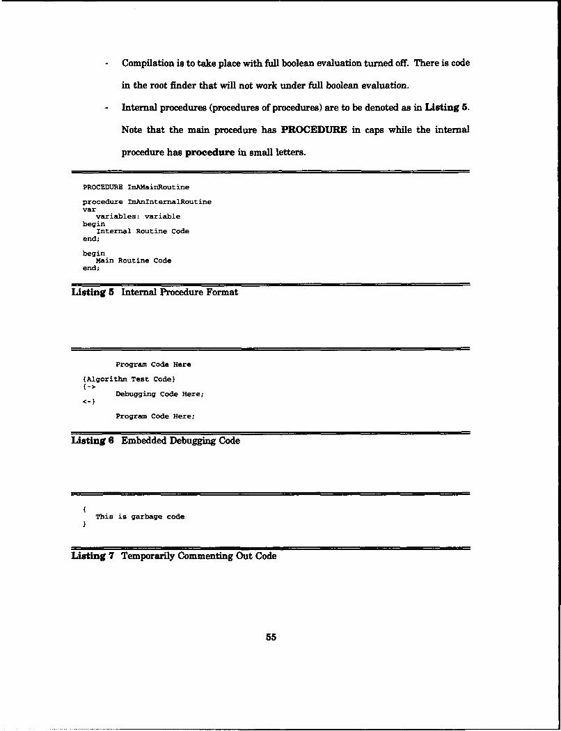
Compilation is to take place with full boolean evaluation turned off. There is code
in the root finder that will not work under full boolean evaluation.
Internal procedures (procedures of procedures) are to be denoted as in Listing 5.
Note that the main procedure has PROCEDURE in caps while the internal
procedure has procedure in small letters.
PROCEDURE ImAMainRoutine
procedure ImAnInternalRoutinevar
variables: variablebegin
Internal Routine Codeend;
beginMain Routine Code
end;
Listing 5 Internal Procedure Format
Program Code Here
{Algorithm Test Code)
Debugging Code Here;
Program Code Here;
Listing 6 Embedded Debugging Code
(This is garbage codeI
Listing 7 Temporarily Commenting Out Code
55
Comments
- Comments are to be denoted with I and ) to facilitate proper software maintenance.
- Code that is temporarily commented out is to have brackets placed on the left
hand margin. For example, Listing 6 shows the proper way to temporarily
comment out unneeded code.
- Embedded debugging code that is left in place is to be commented out as shown
in Listing 7. From this listing, note that the debugging code is commented out
with (-> and <-) placed at the left hand margin. Also note that the debugging code
is indented properly with the normal program code. Finally, the debugging code
is noted with a {Algorithm Test Code) header placed on the left hand margin. The
advantage to using this system is that debugging code is readily activated by
completing the (->I and (<-I symbols.
3.3 Mathematical Specification
The mathematical engine of ICECAP-PC is based on complex arithmetic. This infers
two things. First, this means that the entire data structure of the previous versions of
ICECAP-PC must be redefined as they are based on real numbers rather than complex
numbers. Second, this means that we must allow for the direct entry of complex numbers for
polynomial and transfer function factors (but not their coefficients) and for matrices.
The first requirement to be determined was that of how many significant digits must
internal numbers represent. Specifically, how accurate must numbers be to do discrete 3x3
MIMO QFT for 10 plants when each plant is 10th order with no common terms. How many
significant digits per root or coefficient? Using engineering judgement (Dr Lamont's
experience) and the fact that this is only an educational package, the number of significant
digits for roots and coefficients was specified to be twelve and the maximum order was
56
specified to be twelve also. The problem is that the IEEE extended number data structure can
only provide 19-20 significant digits per number stored. Given ,,.velve 12-significant-digit
roots, thirteen 144-significant-digit coefficients would be needed for exact reconstruction when
moving between root and polynomial form. A simple example helps to explain why this is so.
Assume a polynomial has two roots, -1.12 and -2.43, which are stored in a number format that
maintains three significant digits. The coefficient form of this polynomial would then be found
by multiplying (1.00s + 1.12)(1.00s + 2.43). The resulting coefficients would be 1.00, 3.5500,
and 2.7216. Now assume we want to return to the root form at a later time and we know one
root is -1.12. We know the last coefficient is the product of the two roots, so we simply divide
2.7216 by -1.12 to find the value of the second root, -2.43. Or at least this is how we would
have done it by hand. Remember now that the numbers could only be stored for three
significant digits. Suddenly the three coefficient values become 1.00, 3.55, and 2.72. At first,
this does not seem significant, we only lost 0.0016 off the last coefficient. However, repeat
the dividing of the last coefficient by the known root to find the remaining root and you get
2.72 / -1.12 = 2.42! The actual answer would have been 2.42857... and you would have
expected the computer to round up to 2.43 before storing the answer; however, this would only
be true if your computer was designed to do so, and it probably is not. Thus, approximately
half the significant digits are lost for each multiplication/division pair. Thus, for the above
stated requirements of twelve 12-significant-digit roots, thirteen 144-significant-digit
coefficients would be required. This requirement is not directly obtainable using the IEEE
extended number format and the standard mathematical routines provided by PASCAL. One
solution would be to mimic the solution used in Mathmatica and provide higher significant
digit representation by rewriting all math functions and using a new number format. In effect,
to get one number to represent 144 significant digits, you would use 8 numbers each represent
19 to 20 significant digits. Another solution is to utilize iterative methods when moving
57

between root and polynomial form, using error bounds to gain the required number of
significant digits in reconstruction and to design math algorithms specifically to avoid loss of
significant digits. The latter solution was chosen and implemented.
The other mathematical specification after accuracy is that of scope. The required
scope of ICECAP-PC's mathematical operations is presented in Listing 8. This compendium
Matrix Operations Transfer Function OperationsAddition AdditionAdjoint Domain Conversion (s,z,w')Controllability Matrix L^Hospitals RuleDeterminant MultiplicationEigenvalues Partial Fraction ExpansionEigenvectors (Modal Matrix) SubtractionHermite Normal Form Time Domain ResponseInverse Time Domain EquationLinear Quadratic Regulator Transfer Function to State SpaceMultiplicationObservability Matrix Time Domain AnalysisRank • Figures of MeritResolvent Matrix Responses to InputsScaler MultiplicationState Space to Transfer Function Fretuency Domain AnalysisSubtraction a Bode Plots, InteractiveTranspose Margins (gain and phase)
Nichols Charts, InteractivePolnomia Polar PlotsA ition " Root Locus, InteractivePolynomial Curve Fitting
* MultiplicationSubtraction
Listing 8 Desired Mathematical Capabilities for ICECAP-PC
of capabilities is for the most part simply an inheritance from the previous versions of
ICECAP-PC. Additions have been made to the matrix functions to accommodate the new
MIMO QFr toolbox (which also accounts for the new LAHospitals Rule within the transfer
function capabilities). This scope of function covers a majority of the CACSD capabilities listed
in exhaustive form in [Kheir, 19881.
58
3.4 Human Interface Specification
Section 3.1 lists a set of general goals for an intuitive interface. A set of specific
specifications based on the research reported in Section 2.2 are now given to meet these goals.
They are defined as follows:
3.4.1 Menuing System. The menuing system must allow access to any
command by three ways: (1) a hierarchical menu activated by a mouse or by keyboard, (2) a
toolbar icon activated by a mouse, or (3) by pressing a hot key on the keyboard. The menuing
system must maintain the look and feel of Microsoft Windows 3.1. The menu must be a list
of command words displayed across the top line of the screen. The user selects the desired
command by pointing at the desired command word with the mouse pointer and pressing the
mouse button. This produces a pop-down menu that extends a new list of command words
below the command just selected. If selected, these commands must either produce the desired
output or display a dialogue box prompting for further details before producing the desired
output. If a menu command produces a dialogue box and not immediate output, then the
command word will be followed by an ellipsis (...) to so indicate to the user. Under no
circumstances may the menu levels exceed below the pop-down menus.
Commands that require a certain sequence in activation are made unavailable until
th• user completes the prior commands. This must be conveyed to the user by displaying
unavailable commands in a different color in the menu listings and by making them
insensitive to activation. Also these commands must appear in their chronological order in the
menu listing to assist the user in remembering the sequence of design steps.
The input of large collections of data must be represented in pictorial form whenever
possible. One example of this is a system build function where the user connects icons with
input/output lines and then defines what functions the icons represents. This system build
59
function must be able to drive graphic displays allowing the user easy interaction with the
iterative design process.
3.4.2 On-Line Help. Context sensitive help must be available down to the
command and error message level. The help content should provide instructions for program
use, but should also provide engineering insight into the design process. The system must
allow activation of the help window either by a hot key or icon activation or by menu selection.
Help must appear in a separate window and always allow access to a list of keywords and
topics. By selecting from these lists, the user must be able to read all available help on every
topic.
3.4.3 Data Display. The package must display information in a form which
gives the user insight into the problem being solved. listed information must be orderly and
legible and able to be displayed in graphical form. Graphics should provide full color and high
resolution to not impair the users understanding of the graph.
Because ICECAP-PC is an educational tool, all information must be able to be
presented in a report format suitable for handing in with homework. Session activity should
be separate from large data listings and graphical plots to provide the processor a clearer
understanding of what the student did as opposed to what the student got.
Multiple graphics windows must be allowed to be viewed and updated simultaneously.
All command executions must update all active windows and create new windows if
appropriate. Menus and icons must be accessible during graphics displays allowing the user
to modify model parameters in one window and watch the effects on a display in another
window. Different windows must allow their data to be displayed in different domains (time,
frequency, etc.).
60
3.5 Summary
This chapter lays the foundation for the implementation of ICECAP-PC by giving a set
of specifications for the program. The specifications were first given in general form in
Section 3.1. Here we saw a set of desired characteristics for the ICECAP-PC program. All
of these characteristics will be satisfied in an 00 format. Section 3.2 gives a set of guidelines
for the structure of the code. Section 3.3 lists a set of mathematical capabilities that must
be included in ICECAP-PC. Section 3.4 specified the desired human interface. The interface
itself was not specified because it is dependant on the choice of platform given in Section 4.1.
However, the look, feel and behavior of the interface is clearly specified. These specifications
now form the basis for the development of the program itself.
61
4 Design and Implementation - ICECAP-PC
This chapter describes the design, structure and implementation specifics of ICECAP-
PC Version 10. Discussion covers improving ICECAP-PC 9.0, porting ICECAP-PC 9.OA,
implementing the new user interface, updating mathematical algorithms, and creating a new
macro language. As in any programming project, several design iterations occurred, some
minor and some extensive, such as the change from simple objects to object families and
actors. As the effort progressed, the concept evolved from a very simple model to a more
complex modular model that was required to meet the speed and memory limitations of a
personal computer.
4.1 PASCAL
In way of introduction to this section on design decisions, we start by answering the
overall question of why we chose to use PASCAL. While Ada and C++ were considered viable
options, the decision was made to design ICECAP-PC 10 using PASCAL. [see Section 2.13
in this thesis and Trevino, 19921 This decision was made because Turbo PASCAL 6.0 with
Turbo Vision provides a CASE environment as described by Chikofsky. [Chikofsky, undated]
As such it provides all the software development tools to accomplish the specifications given
in Chapter 3.
A full blown CASE environment, as currently available, is not easy enough to use to
provide the limited time scale of a master's thesis with enough advantages to warrant such
a large expenditure of cash. Furthermore, Lempp and Lauber highlight a specific weakness
in current CASE tools is their inability to provide a graphical representation of program data
flow, function flow, and control flow--the largest problem associated with rewriting ICECAP-PC
9A. [Lempp, undated:1051 However, the underlying goals of a CASE environment are still
62

desirable: to force disciplined techniques in software development, to increase productivity,
and to decrease maintenance required later as the program is modified. [Lempp, undated:1051
The Integrated Development Environment (IDE) within Turbo PASCAL coupled with
the 00 language of Turbo Vision satisfies most of the goals of a CASE environment.
[Chikofsky, undated; Borland, undated; Borland, 1991] The IDE provides a productive
environment in which to write code. The integrated debugger allows the programmer to
single step through the code and watch variable states change while at the same time
watching the program output. The program profiler allows the programmer to optimize
completed code for speed and efficiency by analyzing procedure call frequency, overlay file
access frequency, and disk access frequency, along with other useful datums. The integrated
editor provides a full function word processor to allow quick code writing with minimal
overhead. And at any time during the code writing, the programmer can use the integrated
compiler to find errors in the new code. All of these integrated tools when combined together
into one environment provide the software development tools typically provided by a CASE
environment. However, it is the Turbo Vision package which forces a structured approach on
the code development and provides easy follow-on maintenance and expandability/portability
due to its 00 structure. These are also important aspects of a CASE environment.
Borland Turbo C++ For Windows with Object Vision would have provided the same
IDE and object-orientation. It was initially believed that C++ would make an easier port later
to XWindows on the SUN workstations. However, after analyzing the SUN work station
technical capabilities, it was discovered that XWindows is not at all compatible with Microsoft
Windows. The main problem is with the graphics routines. DOS graphics is done using .BGI
screen driver files and the GRAPH.TPU command unit, but these do not work on a UNIX
workstation which uses ANSII exclusively. Also, the existing ICECAP-PC code was already
in Turbo PASCAL. Thus porting ICECAP-PC 9A into C++ and then later into UNIX would
63
be two very difficult ports, where porting from ICECAP-PC 9A into PASCAL Turbo Vision and
later into UNIX would only be one difficult port. Because time for porting the code had to be
balanced with time required to write the new QFT functions, the decision was made to keep
ICECAP-PC in PASCAL and not convert to C++. Ada was not chosen because there is no
available CASE environment for Ada.
4.2 Object-Orientation
Another introductory design decision was made to implement the new ICECAP-PC
using 00 technology. [refer back to Section 2.1 for details on OOPI
After thoroughly understanding the functional version of ICECAP-PC, it became clear
that a new approach to developing large, complex CAD packages was required. This new
approach would have to ensure that the new code provided modularity to assist follow-on
students in working with the code. It would have ta provide independence of the modules so
that different students could develop different modules at different times. It would have to
provide testability of the modules so that each could be independently validated. And the new
approach would have to ensure reliability of the CAD package as a whole, because a tool that
is not reliable cannot be used by an engineer even for educational purposes. This new
approach was found to be 00 technology.
4.2.1 Modularity. 00 discipline forces modularity on the design through
logical decomposition of the problem into smaller and smaller elements. It brings the modular
programming of PASCAL to its ultimate conclusion. [Pressman, 1987:3361
4.2.2 Independence. With strict modularity, comes the reward of self-
contained modules with a single input and output. Objects force independence through
64

keeping their procedures and data hidden from other objects; no object can directly access the
methods of another object. This is referred to also as encapsulation. [Pressman, 1987:3401
4.2.3 Testability. With a well-defined input/output pair, testability is gained.
It becomes a simple task to apply a test set of inputs and validate proper output responses.
4.2.4 Reliability. After thorough testing, reliability of the module can be
concluded. If all the modules are reliable, the whole program is reliable. Furthermore, with
object inheritance, a piece of code can be reused repeatedly once it has been proven reliable
only once.
These concepts are nothing new to good modular programming in PASCAL; however,
the degree of the discipline is forcibly higher in OOP. OOP also offers a new way of looking
at problem solutions and a new way of grouping up subroutines into tight little bundles called
objects. So along with the traditional values, some new advantages are gained ae well.
4.3 ICECAP-PC 9.0 to ICECAP-PC 9.OA
This investigation begins with the software maintenance task of debugging and testing
the functional version of ICECAP-PC 9.0 and restructuring it into a more modular form in
ICECAP-PC 9.OA. This is done for both transfer function (traditional) and matrix (modem)
portions of the package as well as continuous and discrete portions. This new version of
ICECAP-PC was produced in order to provide a bug-free, algorithmically reliable version of
the functional ICECAP-PC. With this version, the 00 ICECAP-PC could loe developed by just
cutting and pasting in the basic subroutines from 9.0A.
65
4.3.1 Fast Prototyping. Fast prototyping was used both in the past and
current development of the ICECAP-PC code. This is appropriate. Studies have shown that
for "educational" programs, fast prototyping is more suitable than specifying. [Curtis,
undated:2981 Specifically, it was found that prototyping yielded smaller programs which were
lower in functionality and robustness, but easier to use and learn. Also fast prototyping
yielded designs which were harder to integrate with other parts of the software package. The
largest benefit of fast prototyping for thesis students is the absence of the planning and
documentation overhead associated with specifying. However, fast prototyping should not
become an excuse for lazy coding. True use of fast prototyping would be to throw together code
that proves something can be done, and then throwing it all away and design the code from
scratch using the specification method. The method of fast prototyping used in developing
ICECAP-PC is slightly different. The prototype is put together with more care and attention
to detail--less "fast". When the concept is proven to work, the prototype code is polished into
the final product using the IDE.
4.3.2 Unit Decomposition. One problem with the old code was that the
version of Turbo PASCAL which was current when the unit decomposition was accomplished
(version 3.0) only supported units with a maximum compiled size of 64K. The design decision
was made back then to decompose the ICECAP-PC program according to functional
classification--a typical decision made in functional programming. This resulted in a large
number of small units which each contained a large number of routines whose only
relationship grouping them together was a similarity in their function. Thus, all the basic
math routines were grouped in a unit, all the display routines were together, all the frequency
response routines were together, all the time response routines were together, etc. When the
units grew to be larger than 64K, it would be divided into two units, then three, etc. The units
66
grew quickly as the package's power increased. For example, where there was first only an
s-domain frequency response procedure with all its supporting routines in a unit, there later
grew a z-domain routine and then a w-domain routine. As the package grew over the years,
the functional connection between the routines in a unit became more abstract and tenuous,
and thus as a later programmer tried to trace through a high level routine, they found
themselves searching through many units trying to find the location of the procedure called
in the high level routine they were modifying.
4.3.3 Validating the Code. The original plan was to validate the algorithms
in the functional version of the code, so they could be brought directly into the new 00 version
of the code without revision. This goal was unachievable due to an inability to compile the
code within the Integrated Development Environment (IDE) of Turbo PASCAL. The IDE is
the CASE environment we were to use to debug and trace through the algorithms. Memory
limitations and the size of the functional version units would not allow a successful
compilation within the IDE. Therefore, the decision was made to move ahead to the 00
version of the code which, due to the nature of 00 code, would allow use of the IDE.
4.4 ICECAP-PC 9.OA to ICECAP-PC 10
As stated in Section 4.2, ICECAP-PC was to be ported to an 00 structure. Thus,
ICECAP 9.0 was debugged and made more modular to prepare for the port to an 00 structure.
This intermediate version was named ICECAP 9.0A. After 9.OA was completed, the new 00
framework was developed for ICECAP-PC 10.0. Complete details of the initial design of the
00 program structure can be found in a companion thesis. [Trevino, 19921 The original
intent was to completely validate the algorithms within 9.OA and to bring these algorithms
directly into an 00 menuing system and help environment. There were two main reasons this
67

idea was abandoned. First, as stated above, the algorithms within 9.OA were unable to be
validated due to the inability to use the IDE. Second, mixing the two technologies did not
provide a very effective way to marry the two output techniques. The functional output
technique writes directly to the computer screen, erasing anything that gets in the way. The
00 output technique passes information to be displayed to a desktop object which maintains
a windowed environment and writes information to the windows. This same type of
incompatibility prevented any usable way to abort out of a functional algorithm and return
to the 00 menuing system. This hybrid system was tested on users at the 1992 QFT
Symposium at Wright-Patterson AFB, OH but was not well received due to these inadequacies.
Therefore, the decision was made to not only bring the algorithms into the new 00 menuing
environment, but also to recode the algorithms as objects. However, rewriting code takes
considerably more time than validating code when the code was written using the fast
prototyping technique. And it was the extreme prototypical state of the functional ICECAP-PC
code that preempted work in the z- and w'-domains-time was only available to rewrite and
validate the S-domain code.
Because the goal of this thesis effort was to follow all the rules of proper software
engineering, all prototypical code had to be discarded as only "proof of concept" examples, and
the routines completely recoded and validated on a broad range of problem exemplars. This
was achieved for all the S-domain routines in the basic ICECAP-PC package. It was achieved
to a large degree on the MISO toolbox code, and completely on the MIMO toolbox code. It was
also done for the new macro toolbox. In fact, the MIMO and macro toolboxes are the first
toolboxes developed completely during this thesis period, all other modules inherited to some
degree code from the functional version of ICECAP-PC.
We tried to implement the concepts in the paper "In Search of Elegance". [Fisher,
1992:37-461 Elegance maintains that while there are several ways to solve problems, the
68

better way is that way which has tighter code, less confusion, and the more clever solution.
The old ICECAP-PC worked, but it was not elegant. The new 00 version of the code is much
more elegant. The paper also points out that object-orientation in itself does not guarantee
elegance. The author encourages the programmer to not be afraid to throw out objects and
replace them with objects that make more sense, even if it seems like the time designing the
first object is wasted. The time is not wasted, the design just progressed to a higher level with
the first object being an initial design step. We designed many objects which were eventually
eleganced right out of the program. Several math algorithms were coded in several different
ways, with only the most elegant solution remaining in the final code. The root finding
algorithm is probably the largest example of this [reference Section 4.4.6.1 as well as Trevino,
19921.
Our method of elegant fast prototyping was not very successful in designing ICECAP-
PC 9A since the IDE was unavailable to us, but it has proven extremely successful with
ICECAP-PC 10. The difference is the use of our CASE environment (the IDE and Turbo
Vision is discussed in Section 4.1). ICECAP-PC 9.OA would not compile within the IDE due
to memory limitations. These limitations disappeared with the use of OOP; therefore, the
decision was made to not waste valuable design time trying to validate the algorithms without
the use of the IDE tools and to move forward to ICECAP-PC 10. Thus, most of the algorithm
analysis and validation was done, not in ICECAP-PC 9.OA as originally planned, but in
ICECAP-PC 10.0 using our IDE CASE environment. The CASE environment allows
construction of better initial code, and much better polishing techniques for the final code.
With ICECAP-PC 9A the only insight the programmer had into how the code was working was
to put in some WRITELN statements here and there that would dump the internal variable
states from time to time. With ICECAP-PC 10's development inside the CASE environment,
the programmer can see the program output in one window, the variables and their values in
69
another window, and the code statements being executed in a third window. It becomes very
easy to fully understand what the code is doing in such an environment.
One by one the functions were brought into ICECAP-PC 10.0 from 9.OA. This process
involved
(1) globally changing variable names to match the more English-language-oriented
names of 10.0,
(2) creating the data structures for the routine,
(3) creating the object support (broadcast message designators, menubar
commands, etc) for the routine,
(4) providing error handling support for the routine (abort codes and their
associated text messages),
(5) exploring newer algorithms more appropriate for computer environments,
(6) accomplishing white box testing on the algorithm during runtime using the
Turbo Pascal Integrated Development Environment,
(7) accomplishing black box testing on the routine using a page or two of test
cases,
(8) writing macro files to represent the black box examples for ease of use, and
(9) optimizing the compilation of the code for memory and speed.
4.4.1 Variable Names. Extensive translation from nondescriptive variable
names to very long and descriptive variable names was accomplished. For example, the
variable idisangle has now been translated to MISOData^.ObservePhase. This variable
holds the integer value of the phase angle the user wishes to observe during MISO boundary
calculiatins. The use of very descriptive variable names and procedure names provides almost
70
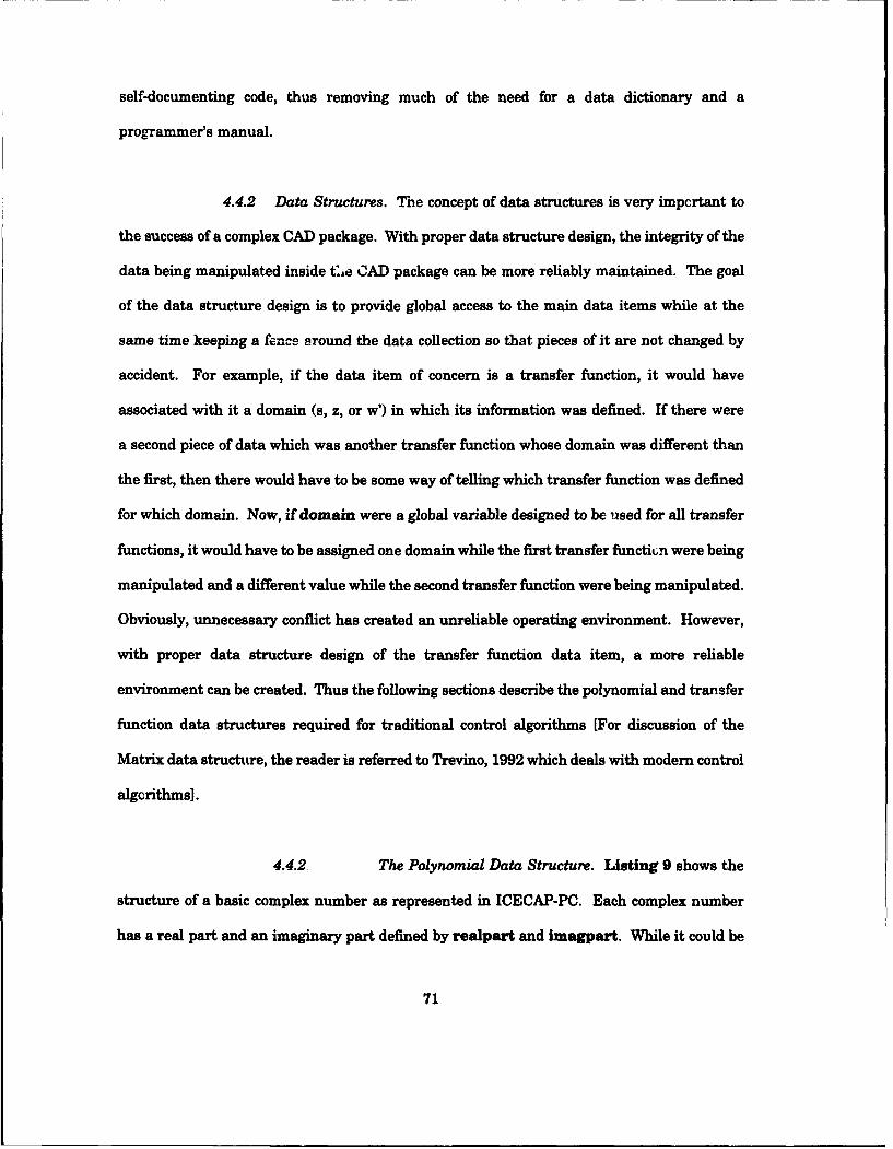
self-documenting code, thus removing much of the need for a data dictionary and a
programmer's manual.
4.4.2 Data Structures. The concept of data structures is very important to
the success of a complex CAD package. With proper data structure design, the integrity of the
data being manipulated inside t.,e C•AD package can be more reliably maintained. The goal
of the data structure design is to provide global access to the main data items while at the
same time keeping a fence around the data collection so that pieces of it are not changed by
accident. For example, if the data item of concern is a transfer function, it would have
associated with it a domain (s, z, or w') in which its information was defined. If there were
a second piece of data which was another transfer function whose domain was different than
the first, then there would have to be some way of telling which transfer function was defined
for which domain. Now, if domain were a global variable designed to be used for all transfer
functions, it would have to be assigned one domain while the first transfer functiun were being
manipulated and a different value while the second transfer function were being manipulated.
Obviously, unnecessary conflict has created an unreliable operating environment. However,
with proper data structure design of the transfer function data item, a more reliable
environment can be created. Thus the following sections describe the polynomial and transfer
function data structures required for traditional control algorithms [For discussion of the
Matrix data structure, the reader is referred to Trevino, 1992 which deals with modern control
algorithms].
4.4.2 The Polynomial Data Structure. Listing 9 shows the
structure of a basic complex number as represented in ICECAP-PC. Each complex number
has a real part and an imaginary part defined by realpart and imagpart. While it could be
71
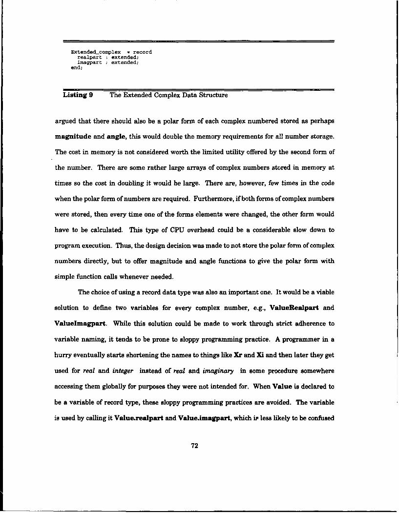
Extended complex = recordrealpart extended;imagpart extended;
end;
Listing 9 The Extended Complex Data Structure
argued that there should also be a polar form of each complex numbered stored as perhaps
magnitude and angle, this would double the memory requirements for all number storage.
The cost in memory is not considered worth the limited utility offered by the second form of
the number. There are some rather large arrays of complex numbers stored in memory at
times so the cost in doubling it would be large. There are, however, few times in the code
when the polar form of numbers are required. Furthermore, if both forms of complex numbers
were stored, then every time one of the forms elements were changed, the other form would
have to be calculated. This type of CPU overhead could be a considerable slow down to
program execution. Thus, the design decision was made to not store the polar form of complex
numbers directly, but to offer magnitude and angle functions to give the polar form with
simple function calls whenever needed.
The choice of using a record data type was also an important one. It would be a viable
solution to define two variables for every complex number, e.g., ValueRealpart and
ValueImagpart. While this solution could be made to work through strict adherence to
variable naming, it tends to be prone to sloppy programming practice. A programmer in a
hurry eventually starts shortening the names to things like Xr and Xi and then later they get
used for real and integer instead of real and imaginary in some procedure somewhere
accessing them globally for purposes they were not intended for. When Value is declared to
be a variable of record type, these sloppy programming practices are avoided. The variable
is used by calling it Value.realpart and Value.imagpart, which if less likely to be confused
72
later and used globally for a purpose for which it was not intended. The advantage of using
record types becomes more pronounced as we get into the polynomial and transfer function
data structures where instead of only having two fields, there are many.
Listing 10 shows the final form of the polynomial data structure. Through extensive
RootPolyType = array[l..MaxDegree] of extended.complex;
CoeffPolyType = array[ 1..MaxDegreel] of extended;
Polynomial = recordname string; {Holds Poly Name)gain extended;degree integer;Factored Root_PolyType;PolyForm: CoeffPolyType;
end;
PolyPtr = ^Polynomial;
Listing 10 The Polynomial Data Structures
experience with the old ICECAP-PC code, it was determined that the pieces of data needed to
fully define a polynomial were as listed. The name field holds a string that uniquely describes
each polynomial. The names used in ICECAP-PC are Polynomial A, Polynomial B, etc. The
gain field holds the value of the gain coefficient for the polynomial. The degree field holds
the order of the polynomial. The Factored field is an array that holds Max-Degree complex
numbers representing the roots of the polynomial. Max-Degree is currently set to 20. The
PolyForm field is an array that holds Max.Degreel numbers representing the coefficients of
the polynomial. MaxDegreel is always one more than Max-Degree. The RootPolyType and
CoeffPolyType are defined separately because they are often needed for temporary variable
types inside routines. The PolyPtr is a pointer variable to a polynomial type and is also
defined separately for use in typing local variables and procedure parameters.
73
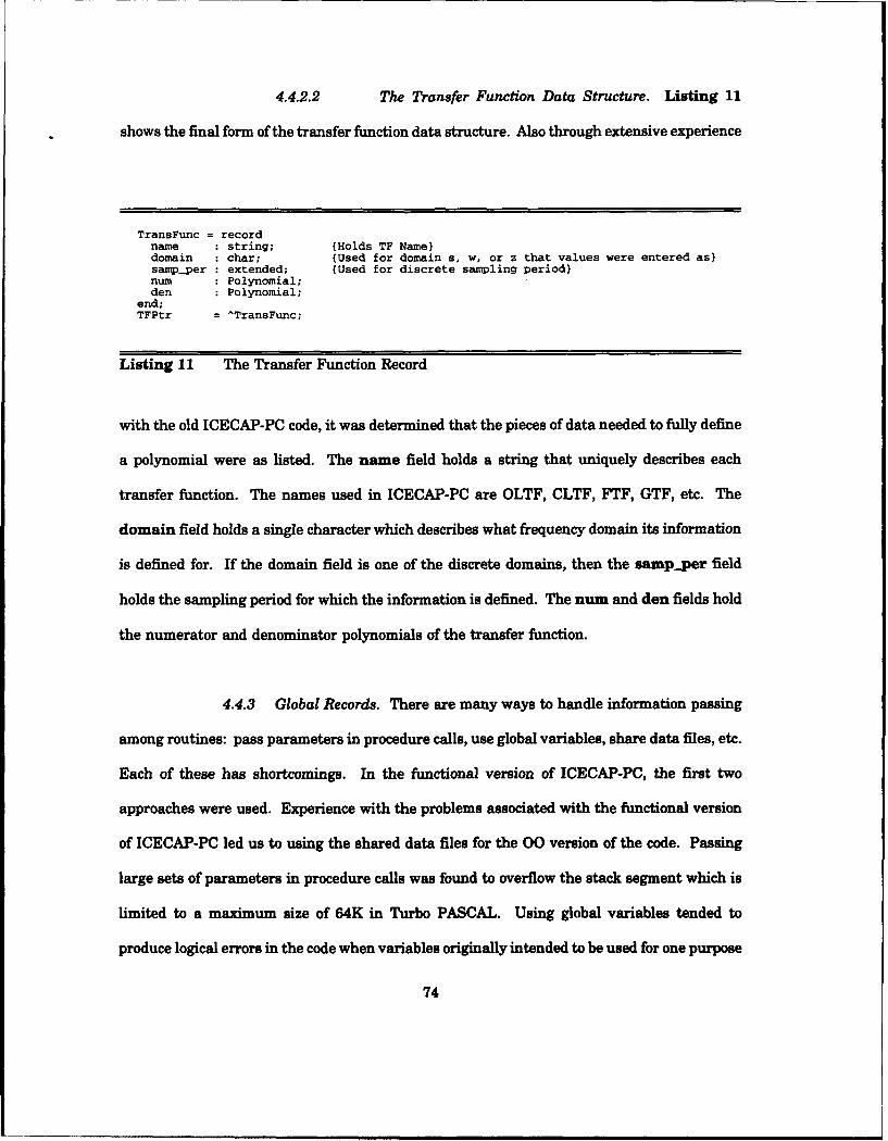
4.4.2.2 The Transfer Function Data Structure. Listing 11
shows the final form of the transfer function data structure. Also through extensive experience
TransFunc = recordname string; {Holds TF Name)domain char; {Used for domain s, w, or z that values were entered as)samp__per extended; {Used for discrete sampling period)num Polynomial;den Polynomial;
end;TFPtr = ^TransFunc;
Listing 11 The Transfer Function Record
with the old ICECAP-PC code, it was determined that the pieces of data needed to fully define
a polynomial were as listed. The name field holds a string that uniquely describes each
transfer function. The names used in ICECAP-PC are OLTF, CLTF, FTF, GTF, etc. The
domain field holds a single character which describes what frequency domain its information
is defined for. If the domain field is one of the discrete domains, then the samp.per field
holds the sampling period for which the information is defined. The num and den fields hold
the numerator and denominator polynomials of the transfer function.
4.4.3 Global Records. There are many ways to handle information passing
among routines: pass parameters in procedure calls, use global variables, share data files, etc.
Each of these has shortcomings. In the functional version of ICECAP-PC, the first two
approaches were used. Experience with the problems associated with the functional version
of ICECAP-PC led us to using the shared data files for the 00 version of the code. Passing
large sets of parameters in procedure calls was found to overflow the stack segment which is
limited to a maximum size of 64K in Turbo PASCAL. Using global variables tended to
produce logical errors in the code when variables originally intended to be used for one purpose
74
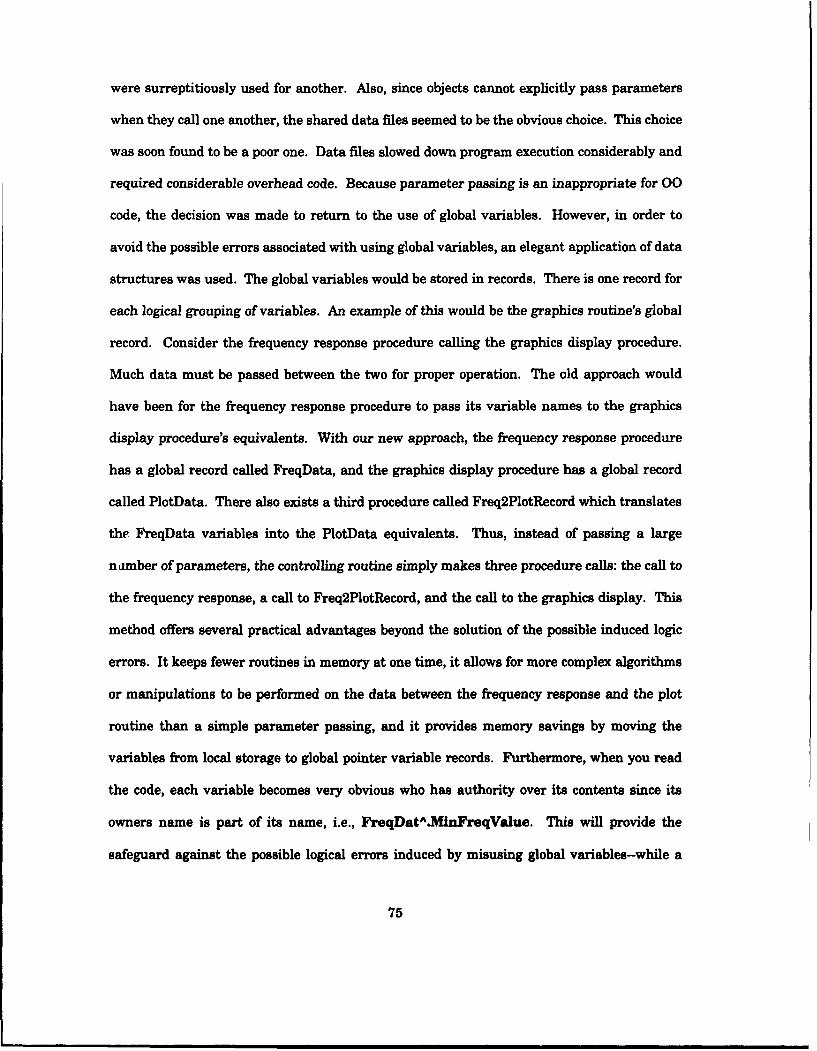
were surreptitiously used for another. Also, since objects cannot explicitly pass parameters
when they call one another, the shared data files seemed to be the obvious choice. This choice
was soon found to be a poor one. Data files slowed down program execution considerably and
required considerable overhead code. Because parameter passing is an inappropriate for 00
code, the decision was made to return to the use of global variables. However, in order to
avoid the possible errors associated with using global variables, an elegant application of data
structures was used. The global variables would be stored in records. There is one record for
each logical grouping of variables. An example of this would be the graphics routine's global
record. Consider the frequency response procedure calling the graphics display procedure.
Much data must be passed between the two for proper operation. The old approach would
have been for the frequency response procedure to pass its variable names to the graphics
display procedure's equivalents. With our new approach, the frequency response procedure
has a global record called FreqData, and the graphics display procedure has a global record
called PlotData. There also exists a third procedure called Freq2PlotRecord which translates
the FreqData variables into the PlotData equivalents. Thus, instead of passing a large
n amber of parameters, the controlling routine simply makes three procedure calls: the call to
the frequency response, a call to Freq2PlotRecord, and the call to the graphics display. This
method offers several practical advantages beyond the solution of the possible induced logic
errors. It keeps fewer routines in memory at one time, it allows for more complex algorithms
or manipulations to be performed on the data between the frequency response and the plot
routine than a simple parameter passing, and it provides memory savings by moving the
variables from local storage to global pointer variable records. Furthermore, when you read
the code, each variable becomes very obvious who has authority over its contents since its
owners name is part of its name, i.e., FreqDatA^MiFreqValue. This will provide the
safeguard against the possible logical errors induced by misusing global variables-while a
75
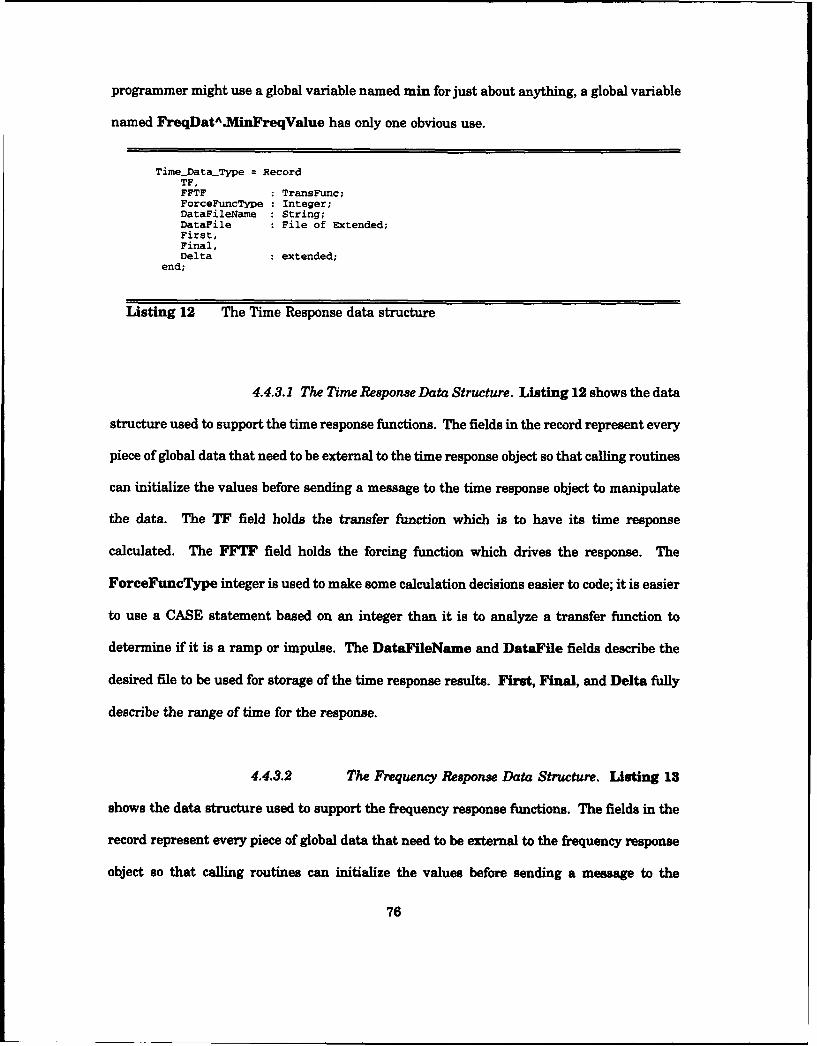
programmer might use a global variable named min for just about anything, a global variable
named FreqDatAMinFreqValue has only one obvious use.
Time_DataType = RecordTF,FFTF TransFunc;ForceFuncType Integer;DataFileName String;DataFile File of Extended;First,Final,Delta extended;
end;
Listing 12 The Time Response data structure
4.4.3.1 The Time Response Data Structure. Listing 12 shows the data
structure used to support the time response functions. The fields in the record represent every
piece of global data that need to be external to the time response object so that calling routines
can initialize the values before sending a message to the time response object to manipulate
the data. The TF field holds the transfer function which is to have its time response
calculated. The FFTF field holds the forcing function which drives the response. The
ForceFuncType integer is used to make some calculation decisions easier to code; it is easier
to use a CASE statement based on an integer than it is to analyze a transfer function to
determine if it is a ramp or impulse. The DataFileName and DataFile fields describe the
desired file to be used for storage of the time response results. First, Final, and Delta fully
describe the range of time for the response.
4.4.3.2 The Frequency Response Data Structure. Listing 13
shows the data structure used to support the frequency response functions. The fields in the
record represent every piece of global data that need to be external to the frequency response
object so that calling routines can initialize the values before sending a message to the
76
FreqRangeType = (LOW, MED, HIGH, USER);
FreaDataType = RecordTF TransFunc;DataFileName String;DataFile File of Extended;FreqArray Array[l..MaxPlotGlb] of extended;FreqArrayString Array[l..MaxPlotGlb] of string[13];FreqRange FreqRangeType;First,Final,Delta extended;HzOrRad,LogOrLinear,MagOrPhase,NormOrDec,NumDecade,NumPoint,PowerOfTen,RadOrDeg Integer
end;
Listing 13 The Frequency Response data structure
frequency response object to manipulate the data. The TF field holds the transfer function
which is to have its frequency response calculated. The DataFileName and DataFile fields
describe the desired file to be used for storage of the frequency response results. The
specification of the range of frequencies for which to take the response is not nearly as straight
forward as the time response is. First of all, FreqArray and FreqArrayltring are required
to hold each value of frequency for which a response point is to be calculated--the array of
numbers is for manipulation, the array of strings is for use in dialog boxes where the user
types them in directly. This preassignment of values is requ•red to provide enough flexibility
for the routines to be used for toolboxes like QFT which only take frequency responses at
discrete frequency points and not over ranges of frequencies. Forcing all toolboxes to assign
a discrete list of frequencies for the response, loses nothing since computer frequency response
algorithms calculate discrete points anyway. What is gained is the generality that a toolbox
which requests a continuous response can fill the discrete array of frequencies using its first,
last, and delta, while with the same routine, a toolbox which requests a response at only
specific frequencies can fill the array with those specific frequencies. The FreqRange field
77
is currently only being used by the MISO QFT toolbox, and allows the user to fill the
FreqArray fields with some default sets of frequencies, if desired. First, Final, and Delta
while no longer used in response calculations are still used in requesting the user's desires and
in parts of the plot routine. HzOrRad if assigned a value of zero signals the user desires
frequencies listed in Hertz. A value of one signals radians/second to be used. This clever
combination of variable name and logical use (Hz or Rad, 0 or 1) is maintained throughout the
ICECAP-PC code, replacing the more common use of boolean flags. This convention makes the
use of global variables more intuitive to the programmer who needs to make calls to the
procedures they are used for. If a boolean was used, the programmer would always be asking
himself whether false meant Hertz or radians/sec. LogOrLinear when assigned a value of
zero signals the user desires any plot to be shown with a logarithmic frequency axis. A value
of one signals a linear axis. If a logarithmic response is requested, then the NumDecade field
holds the number of decades the user desires to have calculated and the PowerOfren field
holds the power of ten at which the user desires to begin the calculation, e.g., 10.1, 102, etc.
If a linear response is requested, then the NumPoint field holds the number of frequencies
to be calculated. This value is, of course, calculated automatically from First, Last, and Delta
and is only stored for ease of coding counter loops within the response procedures. The
MagOrPhase flag is used in the plot routines. ICECAP-PC displays frequency plots as two
separate plots--one for magnitude and one for phase; however, mechanically there is nothing
different between them. The old ICECAP-PC code had separate routines to print magnitude
and phase plots, but using the MagOrPhase flag allows the new ICECAP-PC code to use the
same routine for both. Basically, the frequency response is stored in a 3 position array- the
first position holds the frequency, the second holds the magnitude, and the third holds the
phase. All the flag does is increments the position which is read from the array for the value
axis of the plot. The NormOrDec field communicates the user's desire for normal or decibel
78
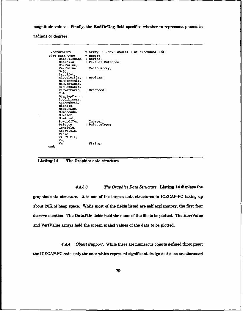
magnitude values. Finally, the RadOrDeg field specifies whether to represents phases in
radians or degrees.
VectorArray = array[ 1..MaxPlotGlbl I of extended; (7k}PlotDataType = Record
DataFileName String;DataFile File of Extended;HorzValue,VertValue VectorArray;Grid,LastPlot,NicColorFlag Boolean;MaxHorzAxis,MaxVertAxis,MinHorzAxis,MinVertAxis Extended;Color,DisplayCount,LogorLinear,MagAngBoth,Nichols,NormOrDec,NumDecade,NumPlot,NunPoint,PowerOfTen Integer;Palette PaletteType;GenTitle.HorzTitle,Title,VertTitle,MM,wm String;
end;
Listing 14 The Graphics data structure
4.4.3.3 The Graphics Data Structure. Listing 14 displays the
graphics data structure. It is one of the largest data structures in ICECAP-PC taking up
about 20K of heap space. While most of the fields listed are self explanatory, the first four
deserve mention. The DataFile fields hold the name of the file to be plotted. The HorzValue
and VertValue arrays hold the screen scaled values of the data to be plotted.
4.4.4 Object Support. While there are numerous objects defined throughout
the ICECAP-PC code, only the ones which represent significant design decisions are discussed
79
herein. For a complete discussion of the design of the ICECAP-PC objects reference Trevino,
1992. The following sections describe the transfer function, time response, frequency response,
graphics, root locus, menu control, and file viewing objects.
4.4.4.1 The TFUNC Object Structure. The TFUNC object
structure is a family of actor objects which handle all polynomial and transfer function
operations. This object is fully addressed in Trevino, 1992.
4.4.4.2 The TIME Object Structure. This object provides all
support for time responses, time equations, figures of merit, and partial fraction expansions.
Methods can be accessed with user interface dialog boxes or directly like procedure calls.
4.4.4.3 The FREQ Object Structure. This object provides all
support for frequency responses. Methods can be accessed with user interface dialog boxes or
directly like procedure calls.
4.4.4.4 The GRAPHICS Object Structure. This object handles
graphics in a vastly more efficient manner than the old ICECAP-PC code. In the first place,
the old ICECAP-PC had extremely large data structures supporting its graphics routines,
while this routines only takes about 20K of data. Further, the methods are modularized so
that the same routines can be called in different sequences in order to produce a plot of a
single function, or a plot of multiple functions. In the old ICECAP-PC, this required
completely separate routines. Finally, all graphics (except the root locus) is done using this
single object and its data structure. This relieves the problem with the old code where each
routine that needed to do graphics had large local variables to hold the data.
80
4.4.4.5 The Root Locus Object Structure. The root locus
algorithms within ICECAP-PC are still based on the Newton-Raphson technique as described
in (Ash, 1968:576-5821 and are among the best on the market. What is new about the root
locus routines in ICECAP-PC is that they are now interactive. The user can move a cursor
using the arrow keys. As the cursor traces along the root locus, it displays the gain and root
position.
4.4.4.6 The Control Object Structure. The Control object
provides a means of memory management. When an object is instantiated, it takes up large
pieces of heap memory. All the Control object does is serve as a central reception point for
messages being passed between objects. When Control receives a message, it instantiates the
receiving object and sends it the message. When the object has accomplished what the
message asked, Control uninstantiates it from memory. The Control object concept coupled
with use of overlay files is as effective at reducing memory requirements as the actor concept.
However, on '286 computers and some slow '386 computers, speed is degraded appreciably
using the Control object. Using both actors and control objects has proven to be the best
solution. The control objects provide the centralized message interface and memory
management, while the small size of the actor objects ensure that speed is maintained.
The Control object also provides a layer of abstraction for toolbox programmers. All
functions in ICECAP-PC are called by sending a message simply to the Desktop. Since the
Control object is instantiated into the Desktop, it receives the message and handles it. What
this means to the programmer is that all they need to know is a listing of messages; they do
not need to know which object handles a message, that is decided within the Control object.
Furthermore, any number of control objects can be instantiated into the Desktop at the same
81
time, so all a toolbox programmer must do to make his object methods accessible to the rest
of ICECAP-PC is provide a control object which handles his message events.
4.4.4.7 The FileView Object Structure. The FileView object is
a full screen editor provided as a part of the Turbo Vision package. It provides a prebuilt
capability for ICECAP-PC to display frequency response listings and other long listings of data
which would otherwise clutter the main viewer window on the ICECAP-PC desktop. It allows
the listings to be saved as any filename the user or program specifies. It also provides editing,
scrolling, and searching of the text. It will even allow opening several files at once. The
limitation is that each file opened be smaller than 64K and that there be at least 100K of heap
space available when the editor is first called.
4.4.4.8 Other Objects. There are several other objects defined
for the traditional control portion of ICECAP-PC. There is a Digital Signal Processing object
and others in differing levels of development. These are not considered important parts of this
thesis effort and are left for detailed coverage within the Programmer's Manual in Appendix
D.
4.4.5 Error Handling Routines. Error handling routines are extremely
important to a user friendly package. It is imperative that the program never crash to DOS
without telling the user why. The ultimate error handling routine would detect the error, trap
the error, try to solve the error itself and continue with the program, or at least send a
message to the user describing what happened and then return to some stable state and
continue with the program. Turbo PASCAL provides the tools necessary to accomplish this;
82
however, the time required to write the routines to handle all the functions in ICECAP-PC
would be impractical for thesis students.
The current solution is to use a global AbortCode variable which is tested after each
function call for an error condition. Each object in ICECAP-PC has a HandleAbort method
which displays an error message box to the user and exits the current procedure. The
limitation of this solution is that it only works for errors that can be detected before the
runtime module aborts to DOS.
4.4.6 Algorithm Improvement. All the basic algorithms which provide the
kernel of math support for ICECAP-PC are rewritten to be more accurate within a digital
computer environment. The algorithms are also optimized for speed and memory requirements
on personal computers. The details of this discussion are provided in a companion thesis
[Trevino, 1992] and are not discussed here. However, there are four topics which are general
enough to be addressed here under this heading: the root finder algorithms, the logarithm plot
algorithms, zero testing, and conditioning numbers.
4.4.6.1 The Root Finder. For a complete discussion of the root
finder upgrade, reference [Trevino, 19921. The root finder is the centerpiece of any CACSD
package. It is important to be able to move between polynomial form and factored form of a
polynomial. There are errors in the accuracy of a given set of roots as well as a reconstruction
inaccuracy in terms of how well those roots can regenerate the original polynomial coefficients.
We have tried to provide some insight to the student as to how accurate the roots currently
being displayed for a polynomial really are. The only way to know the accuracy of the
individual root values is to know what the actual roots are supposed to be. Thus, in real time
operation, the only test for root accuracy is their accuracy in reconstructing the original
83
polynomial coefficients. There are several quick and easy tests that can be used tU detenrine
the coefficient reconstruction accuracy. The two easiest, and the two chosen for
implementation within ICECAP-PC are that (1) the sum of all roots should equal the second
polynomial coefficient and (2) the product of all roots should equal the last coefficient. The
largest of these two errors is then taken as the root accuracy. This raw number can be printed
for the user, or it can be divided by the value of the smallest coefficient and multiplied by 100
to give a percentage error term. ICECAP-PC currently displays the latter.
In order to improve the root finder, first a baseline set of test exemplars was collected.
We used the old code to generate a page of boundary test cases; one example for every order
polynomial, twice, triple, quad, and hept repeated real and complex roots, six to ten repeated
real roots, and all purely imaginary roots. Second, the error bound routine was added to the
old code. Then the error bounds for each of the test cases were generated. Third, the new root
finding algorithms were added to the code and the test cases were rerun to generate new error
terms. The best algorithms could then be chosen based on the error bound results.
The results of the upgrade were mixed. While the old code produced more accurate
roots in examples with several repeated roots, the new code produced extremely better roots
in polynomials with no repeated roots. Further it was found that in the old code while the
roots were not nearly as close to the actual root values as those the new code found, the
reconstruction error terms generated by the code were smailer for the less accurate roots of
the old code. For example, the new algorithm finds roots correctly to 19-20 significant digits,
but the old algorithm only finds them to 8-12 significant digits. However, the reconstruction
errors for the old code were being reported at values suggesting 30-50 significant digits, while
the new code's errors suggested roots with only 10-15 significant digits. The reason for this
disparity phenomenon is that the root errors in the old code were always symmetrical about
the actual root values. If one root is a little less than its actual value, the next root will be
84
a little more than its actual value. Because of these mixed results, both the old and new root
finder algorithms are maintained in the code, and an optimizing algorithm calls both routines
and compares their resulting error terms to determine which roots to accept. This is only a
temporary solution. The more accurate roots of the new algorithm is more desirable for most
modern control techniques using matrices or when doing repeated transfer function
multiplications, while the more accurate factored to polynomial form transition capability is
more desirable for doing most traditional controls algorithms or when doing repeated transfer
function additions.
4.4.6.2 Logarithm Plots. New algorithms for displaying
logarithm plots had to be generated due to the new plot routines. The old routines always
produced the maximum possible number of discrete points along the horizontal axis using
spline techniques. This meant that each point was evenly spaced along the axis, thus the
logarithmic nature of the plot was produced in the routines which generated the valut. -' the
points along that horizontal axis, i.e., it would generate fewer points in the lower part of a
decade and more points in the upper part of a decade so that when it plots, the points are
evenly spaced on the screen. This approach required much overhead in preprocessing data
before plotting and would not allow plotting of discrete values along the horizontal axis-there
always had to be exactly the maximum number of points. The new ICECAP-PC is more
elegant in its approach. Any number of points with any spacing between themn can be sent
directly to the response routines and then to the plotting routines with no preprocessing. The
plotting routines calculate the required location of the data point along the horizontal axis at
plot time based on a simple logarithmic formula. An added advantage of this new approach
to plotting graphics is that the graph produced is a true representation of the points calculated
in the response routines. In the old ICECAP-PC, the spline routines would produce a smooth
85
curve that might mislead the user by producing peak frequencies or rise times that were
simply not true. The results were a function of the number of points generated and the value
of the delta time or frequency used. Future versions of ICECAP-PC will add the spline
smoothing algorithm as a user option.
4.4.6.3 Zero Testing. There were extensive problems in the
algorithms in the old code not testing for zero and causing runtime errors when divide by zeros
occurred. There were further problems with the PASCAL language itself generating floating
point errors when operations were done on zero or near-zero values. This has been taken care
of in the new code by being very careful to do frequent zero testing of variables, and by a bug-
fix/code patch from Borland for our PASCAL compiler. This is discussed in further detail in
Section 6.3.
4.4.6.4 Conditioning Numbers. It was found that a large
number of the runtime errors caused in the old code were due to operations being performed
on variables which had not been initialized to a zero value. While some compilers handle this
task automatically, Turbo PASCAL does not. Therefore, routines were written to initialize
matrices, polynomials, and transfer functions to zero values.
Another aspect of conditioning numbers is that of truncation. Even though extended
number types within PASCAL can represent numbers as small as 3.4E-4932, the algorithms
and mathematical functions cannot practically operate at these accuracies since they can only
maintain 19-20 significant digits. What this means is that there can be significant
quantization error introduced into mathematical results. We found that setting the arbitrary
floor on numerical representation at 1E-100 tended to produce more precise answers.
Basically, the way this floor is used is to condition operands before an operation and the
86
results afterwards. To condition a number, you simply set it equal to 0.0 if it is less than 1E-
100. In the root finder, we even go so far as to truncate all fractional parts of numbers below
1E-100. This tends to keep the root finder more stable. An interesting note is that the old
ICECAP-PC truncated fractional parts of roots below 1E-6, even for discrete domains. The
problem with setting these arbitrarily assumed floors is that someone's entire design might
exist at values of very small magnitude poles--especially in a discrete design. The simple
solution is to keep the user informed through help screens about any assumptions like these
which are made. All they would have to do is simply scale all their design values by a few
orders of magnitude to bring it back up to a level which is practical on a computer. Obviously,
1E-100 is not a pragmatically provable optimum number, and future thesis work should
include some analysis of performance improvements by tweaking this global number.
4.4.7 Unit Decomposition. With the newer version of Turbo PASCAL
allowing units larger than 64K and with the use of OOP, the newer version of ICECAP-PC
offers a decomposition that is easier to use and maintain. In the first object decomposition of
ICECAP-PC, there were basically three objects: Matrix, TransFunc, and Graphics [ for a
complete object decomposition reference Trevino, 1992, but for this discussion it is accurate
enough to only refer to the three main objects). Each object was defined by two units. One
unit held the object definition along with all the user interface overhead, and one unit held the
basic math routines associated with the object. This dual unit concept provided a single unit
to contain the 00 support for the menu system, and a single unit to be used by new toolboxes
for lower level math support. For example, the code inside the main ICECAP-PC program to
handle menubar requests for a frequency response would generate a message to the TransFunc
object inside the TransFunc unit. The TransFunc object would then produce a dialog box to
allow the user to select which transfer function to display a response for and how to display
87

the results. However, the code inside the MISO QFT toolbox to handle menubar requests for
template generation would generate a message to whatever object handles template generation
and would display a dialog box appropriate to that function. But when that object began to
calculate the templates and needed to generate frequency responses for them, it would directly
call the frequency response procedure inside the PolyTFMath unit. The TransFunc object
would thus be avoided so that no dialog boxes concerning frequency responses are generated.
This dual unit decomposition was later decomposed further into actors. [Trevino, 1992]
The actors are just a further object decomposition of the three major ICECAP-PC objects into
three object families. For example, instead of having the Matrix object contain methods for
MatrixAdd and MatrixMultiply, the methods were made objects themselves. Thus the basic
Matrix object is called MatrixBasic, and the MatrixAdd method was made a child object of
MatrixBasic and is called MatrixAdd. Each of these new actor objects are stored in their own
units. Thus MatrixBasic is stored in unit MatBasic (the name was shortened to be a valid 8-
character DOS file name), and MatrixAdd is stored in unit MatAdd. The advantage of these
single-method objects and single-object units is speed. The small units make the time required
to swap the units in and out of the overlay file very short. And while the number of unit files
on disk is very large, the naming convention being very similar to the actual method name
avoids the old confusion of wondering what unit a certain method is stored in.
4.4.8 Compiler/Memory Issues. The basic ICECAP-PC CAD package
represents 1155 compiled lines of code and almost 500K of executable code. If one includes
all the toolboxes, the package has over 1 Meg of executable code and almost 1.5 Meg of
PASCAL programs. It is obvious that some type of magic must be worked to get a 1 Meg
program to execute in the 640K that a PC offers any program. This magic is worked by the
PASCAL compiler. Through a combination of overlays, actors, control objects, pointer
88
variables, and expanded memory, an ICECAP-PC CAD environment is created that can offer
the user a library of toolboxes that are unlimited by size or number. The following paragraphs
discuss this compiler magic.
There is considerable trade off in the compilation structure of ICECAP-PC. The
slowest XT can run ICECAP-PC, but we can lessen the amount of overlays and compile
without 286 instructions to improve reliability and speed on the underpowered XT processor.
A 486 on the other hand can take full advantage of expanded memory overlays and special
compiler instructions to maximize available heap to solve larger problems.
The more we overlay during compilation time, the more heap space that is available
for larger order transfer functions, etc. The display buffer size, maximum number of response
values, maximum screen resolution, maximum order or transfer functions and matrices, etc.
are all chosen arbitrarily at compile time. This allows ICECAP-PC to be tailored for individual
use. In fact, through the control objects, one could delete every other function of ICECAP-PC
and its toolboxes quickly and easily to allow only one type of problem to be solved. This would
free up enough heap space to maybe double or triple the maximum order of the problem to be
allowed.
Many lessons were learned about which parts of ICECAP-PC could be put into overlays
to free up heap space. It was found through the use of the Turbo Profiler that overlaying the
basic Turbo Vision units such as App, Memory, Objects, Dialogs, Menus, and Views would give
50K of additional heap space, but only at the sacrifice of severe overlay access--thus slow
response--on 286 machines. Also overlaying any unit whose .TPU file compiled to more than
64K also severely slows down the system. Also any unit accessed in the ICECAP-PC.IDLE
routine should not be overlaid or a constant disk read results from swapping in and out that
unit. Furthermore, sending broadcasts simply to the Desktop requires every single unit to be
read in from the overlay one at a time to see how it responds to the broadcast. For this
89
reason, it is best to specify one unit in all broadcast commands. Finally, storing the overlay
file in expanded memory or on a RAM disk vastly improve performance.
In addition to the use of overlays, is the use of actors and control objects discussed
previously. By applying all the tricks we have learned, it is possible to run ICECAP-PC in as
little as 100K of RAM. This is quite an achievement for a package of such power, and makes
ICECAP-PC very portable over personal computer platforms--XTs, laptops, etc. However, the
best performance is produced by running ICECAP-PC in 640K of RAM with a few hundred
kilobytes of expanded memory available for the overlay files. With the new Borland PASCAL
7.0 discussed in Chapter 7, it becomes possible to avoid the 640K RAM barrier and run
ICECAP-PC in up to 16 Meg of RAM. This is due to Borland PASCAL's new ability to exploit
the protected mode of the new '386 and '486 CPUs.
4.5 User Interface Development
4.5.1 The Menuing System. Figure 2 shows the friendly user interface Turbo
Vision has enabled ICECAP-PC to provide. Every command within ICECAP-PC can be
accessed through a single-level pull-down menu system. The matrix pull down menu is shown
as an example in Figure 3. The internal mechanics of the menus are very simple to
implement for the programmer. For every key word shown on the menus, there is a
corresponding hot key specified (Fl, Alt-X, etc), a help context topic (hcFrequencyResponse,
hcFileOpen, etc), and a command word to generate (cmFrequencyResponse, cmfileOpen, etc).
When the user clicks the right mouse button on a menu item, the help context topic is sent to
the help object which then displays the relevant help dialog boxes for that menu item. If the
left mouse button is clicked on the menu item, its command word is sent to the ICECAP-PC
HandleEvent method. The HandleEvent method then searches a large CASE statement to find
what action should be taken to respond to the user's selection of the menu item. Typically this
90
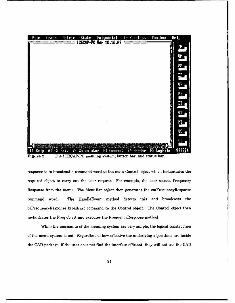
ICECAP-PC Uer IA.i0.9
Figure 2 The ICECAP-PC menuing system, button bar, and status bar.
response is to broadcast a command word to the main Control object which instantiates the
required object to carry out the user request. For example, the user selects Frequency
Response from the menu. The MenuBar object then generates the cmFrequencyResponse
command word. The HandleEvent method detects this and broadcasts the
brFrequencyResponse broadcast command to the Control object. The Control object then
instantiates the Freq object and executes the FrequencyResponse method.
While the mechanics of the menuing system are very simple, the logical construction
of the menu system is not. Regardless of how effective the underlying algorithms are inside
the CAD package, if the user does not find the interface efficient, they will not use the CAD
91
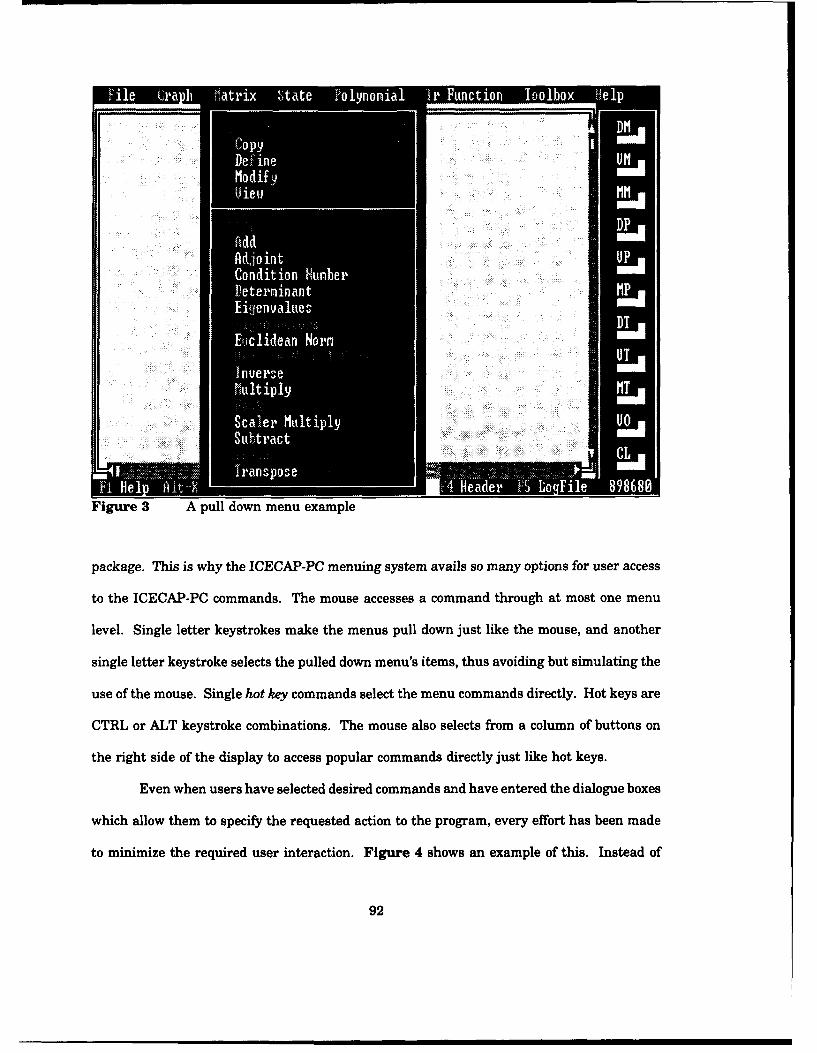
De i n3 I
Figure 3 A pull down menu example
package. This is why the ICECAP-PC menuing system avails so many options for user access
to the ICECAP-PC commands. The mouse accesses a command through at most one menu
level. Single letter keystrokes make the menus pull down just like the mouse, and another
single letter keystroke selects the pulled down menu's items, thus avoiding but simulating the
use of the mouse. Single hot key commands select the menu commands directly. Hot keys are
CTRL or ALT keystroke combinations. The mouse also selects from a column of buttons on
the right side of the display to access popular commands directly just like hot keys.
Even when users have selected desired commands and have entered the dialogue boxes
which allow them to specify the requested action to the program, every effort has been made
to minimize the required user interaction. Figure 4 shows an example of this. Instead of
92
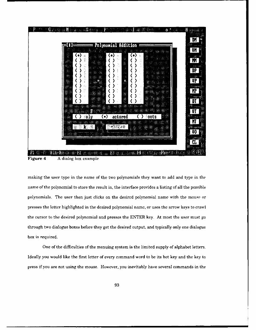
W ýactoredm
Figure 4 A dialog box example
making the user type in the name of the two polynomials they want to add and type in the
name of the polynomial to store the result in, the interface provides a listing of all the possible
polynomials. The user then just clicks on the desired polynomial name with the mouse or
presses the letter highlighted in the desired polynomial name, or uses the arrow keys to crawl
the cursor to the desired polynomial and presses the ENTER key. At most the user must go
through two dialogue boxes before they get the desired output, and typically only one dialogue
box is required.
One of the difficulties of the menuing system is the limited supply of alphabet letters.
Ideally you would like the first letter of every command word to be its hot key and the key to
press if you are not using the mouse. However, you inevitably have several commands in the
93
mmm • nm() ()m
same menu that start with the same letter. The solution is to either think of other command
words that mean the same thing and start with unique letters or use the second, third, or last
letter to specify that command word. Another difficulty was found with the hot keys. Turbo
Vision only supports recognition of the ALT key. The plan originally was to have each main
pull down menu to have its own key designation. For example, every command in the Matrix
menu could be accessed by pressing the Alt key and the letter of the matrix command word
desired, whereas every command in the Transfer Function menu could be accessed by using
the CTRL key. However, with eight main pull down menus, the supply of unique hot keys was
soon used up. With some research, it was found that the Left Shift, Right Shift, ALT, and
CTRL keys as well as any combination of the four could be detected in Turbo Vision with some
fancy coding in the Get Event. This was not given a high priority, and is thus left for future
development.
Even the appearance of the menuing system was studied and made as aesthetically
pleasing as possible. The colors were selected based on proven HFE knowledge on the impact
of colors on the human mind. [Smith, 1986:180-1861 The main menu commands were all
selected to be nouns with all the pull down menu commands being verbs. This has been found
to be the most understandable interface for humans. [Smith, 1986:23'-247] In the ICECAP-
PC package the menu commands were ordered alphabetically since the order is not as
important as speed of finding the desired command. But in the current QFT toolboxes, which
are more tutorial in nature, it was important for the user to have the commands in the
chronological order in which the QFT design method demands them to be executed. The menu
was also placed on the top of the screen instead of to the side. A status bar is always kept
visible at the bottom of the screen. A toolbar is always kept visible to the right of the screen.
Further, the attempt was made to make the menuing system as intelligent as possible.
In the old ICECAP-PC, if the user requested a graph of a frequency response that had not yet
94
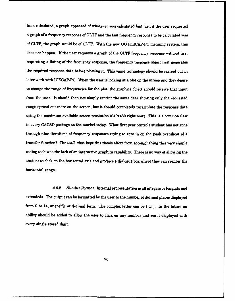
been calculated, a graph appeared of whatever was calculated last, i.e., if the user requested
a graph of a frequency response of OLTF and the last frequency response to be calculated was
of CLTF, the graph would be of CLTF. With the new 00 ICECAP-PC menuing system, this
does not happen. If the user requests a graph of the OLTF frequency response without first
requesting a listing of the frequency response, the frequency response object first generates
the required response data before plotting it. This same technology should be carried out in
later work with ICECAP-PC. When the user is looking at a plot on the screen and they desire
to change the range of frequencies for the plot, the graphics object should receive that input
from the user. It should then not simply reprint the same data showing only the requested
range spread out more on the screen, but it should completely recalculate the response data
using the maximum available screen resolution (640x480 right now). This is a common flaw
in every CACSD package on the market today. What first year controls student has not gone
through nine iterations of frequency responses trying to zero in on the peak overshoot of a
transfer function? The wall that kept this thesis effort from accomplishing this very simple
coding task was the lack of an interactive graphics capability. There is no way of allowing the
student to click on the horizontal axis and produce a dialogue box where they can reenter the
horizontal range.
4.5.2 Number Format. Internal representation is all integers or longints and
extendeds. The output can be formatted by the user to the number of decimal places displayed
from 0 to 14, scientific or decimal form. The complex letter can be i or j. In the future an
ability should be added to allow the user to click on any number and see it displayed with
every single stored digit.
95
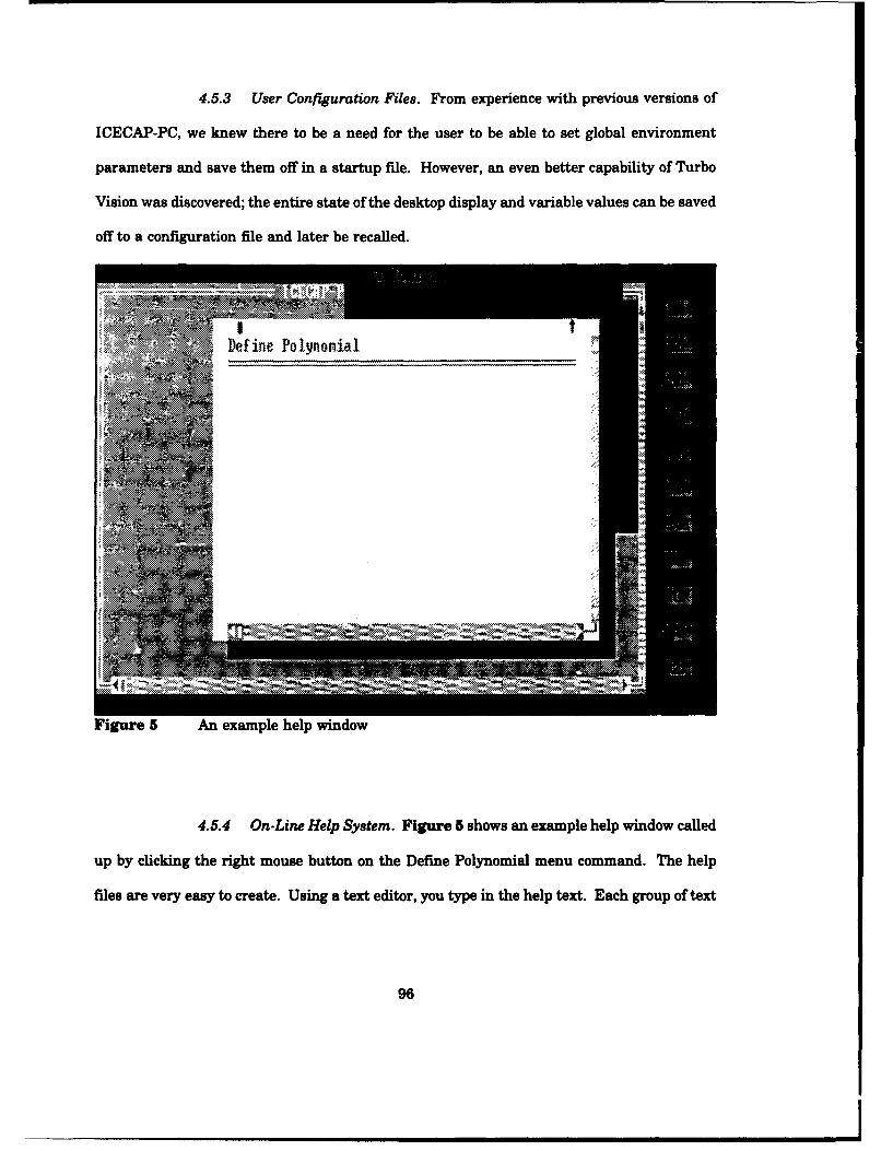
4.5.3 User Configuration Files. From experience with previous versions of
ICECAP-PC, we knew there to be a need for the user to be able to set global environment
parameters and save them off in a startup file. However, an even better capability of Turbo
Vision was discovered; the entire state of the desktop display and variable values can be saved
off to a configuration file and later be recalled.
Define Polynonial
Figure 5 An example help window
4.5.4 On-Line Help System. Figure 5 shows an example help window called
up by clicking the right mouse button on the Define Polynomial menu command. The help
files are very easy to create. Using a text editor, you type in the help text. Each group of text
96
on a certain topic is started with a keyword which ties it to a menu command or dialog box.
Then a separate help compiler is run on the help file to produce a runtime help system file.
It is important that these help files not only contain information on how to use the
program and the allowed format of entries, but also information to educate the user. This type
of information includes engineering rules of thumb for design, the formulae used by the code
for the chosen algorithm, assumptions made in the chosen algorithm, as well as the AFIT
professor engineering experience and insight into the design process. With this type of on-line
help, ICECAP-PC would be more valuable than any commercial package for its help system
alone regardless of how well it cranked out answers to problems.
4.5.5 Data Presentation. Several breakthroughs were made in the area of
designing ICECAP-PC's routines for data presentation. These include session logging, data
listings, and interactive graphics.
As discussed in Section 3.4.3, it is important that output reports produced by an
educational package be different than those produced by commercial packages. The professor
must be able to easily separate session log files from long data listings and graphics plots. By
keeping these separate, he can determine what the student did to produce the incorrect
answers in the listings and plots. ICECAP-PC has been designed to provide that separation
[Trevino, 1992]. The session logging function within ICECAP-PC, shown in Figure 7, first
allows the student to put a header at the beginning of the session file which displays his name
and the class and session information. The logging function then pipes all data displayed in
the main display window to an ASCII file whose format is exactly as it appears on the
computer screen. During this log, the student can enter directly any comments he might want
to make about what is on the screen. When a long listing, such as a frequency response, is
produced by ICECAP-PC, the output is not listed in the main window but in a full screen
97

F1 ie a-G Matrix State P3lComi n Ia F4 unction Tool oxe p• e
Waynre 6B All o fieexm
Std ento widw ssoni iur .A rt"suetha de n omnso
Trvies trany sferfulotions suh pssroblemn a.3 isgiearhng Feor- a ldsuso fth
3.itor (ucinsee Scion 4.4.4.+7.000 Whnagahcceni rdcd h tdNt a sn
(s + 2.00tj.00)S+400)D
it All thisrinte being loggerna ator packaext f vile l wtIEC -P b UTnopatf
-U
Figured inteActgie examphissresaeasoaalbewtieIEA-Ceea
etdentor voinedow as affhtown inFigro.Atr the studendPrgamC ot hacs adddnyctommnt wihsows
formatstiong othe desies, hn er csyucangsae the fiegoanainvamuehhoe. Thinew fulltereien grapitor
Seveilty ral ineatvbgahcceens adde als avilbeheti ICECAP-PC. rotcsruies lonwpo evueralo
98
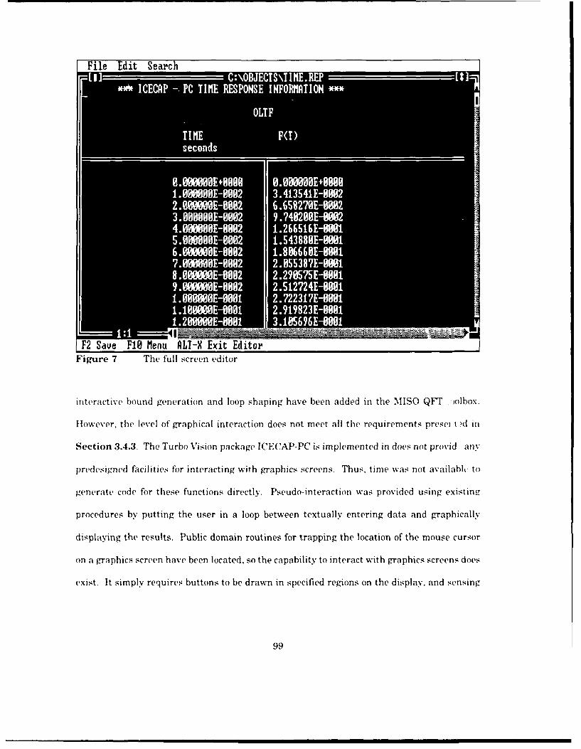
File Edit Search
Figure 7 The full screen editor
interactive bound generation and ioop shaping have been added in the MISO QFT , olbox.
Htowev'er, the level of graphical interaction does not meet all the requirements presei t d in
Section 3.4.3 The Turbo Vision package ICECAP-PC is implemented in does not provid any
predesigned facilities for interacting with graphics screens. Thus, time was not availabh, to
generate code for these functions directly. Pseudo-interaction was provided using existiniz
procedures by putting the user in a loop between textually entering data and graphically
displaying the results. Public domain routines for trapping the location of the mouse cursor
on a graphics screen have been located, so the capability to interact with graphics screens does
exist. It simply requires buttons to be drawn in specified regions on the display, and sensing
99
when that region is activated by the mouse. Then all that is left is writing procedures to
produce the function associated with each button on the screen.
4.6 Summary
This section has discussed the design, alternatives, and implementation of the
ICECAP-PC program. Section 4.1 discussed the decision to used Borland Turbo PASCAL
with Turbo Vision as the language to implement the design in. Section 4.2 reiterated the
importance of object-orientation to the code design. The code development from ICECAP-PC
9.0 to ICECAP-PC 9.OA was presented in Section 4.3. Section 4.4 contains the bulk of the
text of this section. It describes the design decisions made in porting ICECAP-PC 9.OA into
the 00 version 10. The user interface implementation is deliberated in Section 4.5.
100
5 Toolbox Design and Implementation - MISO QFT
This chapter describes the design, structure and implementation specifics of the MISO
QFT Toolbox. First the toolbox concept is discussed in terms of why it was chosen, then the
MISO QFT toolbox design is discussed.
5.1 The Toolbox Concept
The toolbox idea is meant to make ICECAP-PC infinitely expandable. Reference
Section 1.3.3 for a detailed discussion of the utility of the toolbox concept. For the design of
toolboxes, there are two possible approaches: (1) make each toolbox a separate .EXE file, or
(2) make each toolbox a separate object.
If option 1 is used, the toolbox program is run using the EXEC command inside the
ICECAP-PC HandleEvent when the toolbox is chosen from the ICECAP-PC menubar. The
.EXE file creates its own desktop and menubar and global variables; in fact, the main
ICECAP-PC program is not even executing. One advantage of this option is it provides the
highest level of independent compiling between ICECAP-PC and its toolboxes. Indeed, there
are no references at all within ICECAP-PC to anything regarding the toolbox. Another
advantage is that if the toolbox is unavailable, a dummy .EXE file can easily be substituted
and print some type of nonavailability message. The primary disadvantage is that data is
shared only through data files saved to disk. The other disadvantage is that this option uses
much more memory than option 2 because there is twice the heap overhead in memory at one
time since both programs are held in memory at once.
If option 2 is used, the toolbox object is called like any other object, except it replaces
the menubar and button bar with its own. Its disadvantage is that this swapping must be
done inside the ICECAP-PC code, so independent compiling is not possible. An advantage to
this option is that data is shared through common global variables as well as data files.
101
Another advantage is that memory use is very efficient because the toolbox object requires very
little overhead memory, and its unit can be put in ICECAP-PC's overlay file.
The decision was made to use both options in order to gain the advantages of both.
During code development, the toolboxes are developed as separate .EXE files. This provides
more memory space for the IDE tools to operate, as well as keeps the developing code
completely separate from the finished ICECAP-PC product. Once the toolbox has been
completely written and tested, the toolbox object definition can be made a part of ICECAP-PC.
This is a simple transition, so there is little overhead time involved by using both options. The
PASCAL file is changed from a PROGRAM file to a UNIT fie with the change of a single file
header word and the addition of an INTERFACE and IMPLEMENTATION section. The
toolbox object is then changed from being a child of TApplication to being a child of TView.
With a slight modification to the INIT method, the new toolbox object is part of the ICECAP-
PC object family.
5.2 The MISO QFT Toolbox
As the focus of this thesis effort, a Multiple-Input-Single-Output (MISO) Quantitative
Feedback Theory (QFT) toolbox was created. This toolbox allows manual, interactive, and
automatic QFT design for continuous, linear, time-invariant MISO control systems problems.
The implementation of this toolbox is discussed in the following sections.
In way of introduction, I will first offer some motivation as to why we needed to create
yet another MISO QFT package since several very fine packages already exist. [Bailey, 1992;
Sating, 1992; Yanev, 1992] First, it was desired to have a package which kept its menuing
system, help text, and output true to the standard terminology offered by [Houpis, 1992c].
Second, it was desired to have a package which offered the user several different design
approaches instead of just being a demonstration of the author's newly discovered
102

methodology. Also these different design approaches should include options to enter the design
data directly, allow interactive design, or produce a fully automatic design. Third, it was
desired to have a package which remained true to Dr Horowitz's original concepts and the
methods one would need to solve the problem by hand--the basis for ICECAP-PC is not to solve
a problem, but to teach the user how to solve a problem. An example of this would be the way
several packages abandon the concept of the UHFB for the more advanced method of
calculating tangencies between the desired ML contour and each template. While this is a good
technique for computer packages to offer, and ICECAP-PC will offer it as an option, the
student must be shown how the UHFB works. Fourth, no other MISO QFT CAD package is
based on 00 technology, and we desired to see if object-orientation offered any new insights
into the design algorithms or data displays. Finally, it is the goal of AFIT to spread the use
of the QFT method as wide as possible. Because ICECAP-PC already has a very large
international user base, it was desirable to offer a public domain QFT extension to ICECAP-
PC.
5.3 The MISO Process
A complete explanation of the QFT MISO design process (of which this is a summary)
can be found in the QFT Toolbox User's Manual in Appendix E of this thesis. For brevity's
sake and to avoid useless repetition, only the philosophy behind the process is discussed here
in the thesis body.
Above all other goals the author holds for the QFT MISO Toolbox is that it teaches the
user how to do basic QFT design by hand. The danger in automating a design process to the
level of leaving out the human entirely is the same danger in giving a loaded shotgun to an
infant who does not understand what it is for or how to use it safely. It is only fruitful for a
computer program to handle the mundane detailed calculations of a long design process, if the
103

human could have done them by hand if they had the time. If the user could not do it by
hand, then they do not have the insight into the assumptions and tradeoffs made by the
computer to ensure the final design is adequate. It is this belief that has driven the design
of the MISO QFT toolbox. Whenever possible (time permitting) three approaches to each
design step have been included: (1) the user accomplishes the design by hand and enters the
results directly, (2) the user interactively accomplishes the design with the computer package,
and (3) the computer package accomplishes the design with no user involvement.
Furthermore, the help screens for each step include insightful information into the formulas
and algorithms used, assumptions made, tradeoffs made, etc.
Another design goal was to keep the design process true to Dr Horowitz's methods.
[Horowitz, 19811 An example of this would be the way the package handles the use of the
Ultra High Frequency Bound (UHFB) and the choice of the nominal plant. [Ballance, 1992:741
The purpose of the UHFB is to guarantee stability of the design at high frequencies, and the
choice of the nominal is to give a point to design for to insure that none of the template
intersects the specified ML contour. With the computational power available to today's
computers, it would have been possible to eliminate the need for the traditional UHFB by
simply using tha -act ML contour specified and doing many more computations than possible
by hand in ensuring that no plants intersect the ML contour. However, the goal is to teach
students to understand the concepts, not to find the least conservative design, so the UHFB
is left in the design process. Further, it is commonly not mentioned in text books [see [D'Azzo,
1988:7041 and their reference to [Horowitz, 19811 for example, also [D'Azzo, 1988:728]] that
the choice of the nominal plant is not random. The later Houpis & Lamont text makes the
point that the nominal plant must be the plant from the given set of plant variations with the
smallest magnitude and most negative phase. [Houpis 1992, 541] However, no explanation
is given that this choice is so the UHFB can be used as the actual stability bound. [Ballance,
104
1992:761 If any other nominal plant were chosen, the UHFB would have to be calculated very
differently. [Houpis, 1992:532] The template would have to be moved all around the specified
ML contour and the points of tangency would be the top of the ashcan. The vertical portion
of the ashcan would be the old UHFB plus the distance from the correct nominal point to the
selected nominal point. Figure 8 illustrates this. If the nominal plant is chosen to be the
most negative phase and lowest magnitude point on the template (lower lefthand corner) then
the ML contour becomes the top of the stability bound since the nominal point moves tangently
right along it. And if the templates become a simple straight line of height V at very high
frequencies, then the bottom of the stability bound would be the bottom of the ML contour
lowered by V distance, thus forming an ashcan shape. While ICECAP-PC does not allow the
student to choose any point as the nominal other than the one just discussed, part of the
toolbox design process presents this issue to the student.
The ashcan form of the stability bounds used in ICECAP-PC is not always valid. One
example is if a MIMO design uses different phase margins for each row of the plant matrix,
then the templates at very high frequencies do not tend to a vertical line. They have widths
which are a multiple of 90 degrees. [D'Azzo, 1988:7061
The toolbox is rather unique in the variety of ways the plant variations can be
generated. The student can enter the plant transfer functions directly, specify coefficient
variations, or specify pole/zero variations, or specify the latter two combined with convex hulls
as discussed in the following paragraph. Each of the functions are pretty obvious how they
would be implemented, however, it is perhaps not so obvious if these variations actually
generate a valid set of plants. Given a transfer function 1 / (s2 + as + b), and the specification
that 'a' and V' vary between 1 and 5, how can one prove that selecting a set of 25 plants (one
for (a,b) = (1,1), (1,2) ... (1,5) ... (5,5)) provides a valid controller designed to satisfy those 25
plants. Perhaps the 26th plant would have been invalid for the designed controller. Perhaps
105
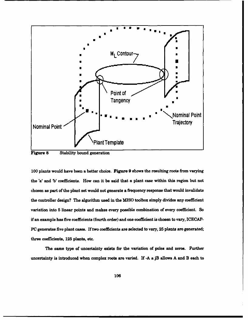
U U
U U
• * MLContour"
*• Tangency
f * 0 "--,Nominal Point
Nominal Point Trajectory
PlantTemplate
Figure 8 Stability bound generation
100 plants would have been a better choice. Figure 9 shows the resulting roots from varying
the 'a' and W' coefficients. How can it be said that a plant case within this region but not
chosen as part of the plant set would not generate a frequency response that would invalidate
the controller design? The algorithm used in the MISO toolbox simply divides any coefficient
variation into 5 linear points and makes every possible combination of every coefficient. So
if an example has five coefficients (fourth order) and one coefficient is chosen to vary, ICECAP-
PC generates five plant cases. If two coefficients are selected to vary, 25 plants are generated;
three coefficients, 125 plants, etc.
The same type of uncertainty exists for the variation of poles and zeros. Further
uncertainty is introduced when complex roots are varied. If -A ± jB allows A and B each to
106
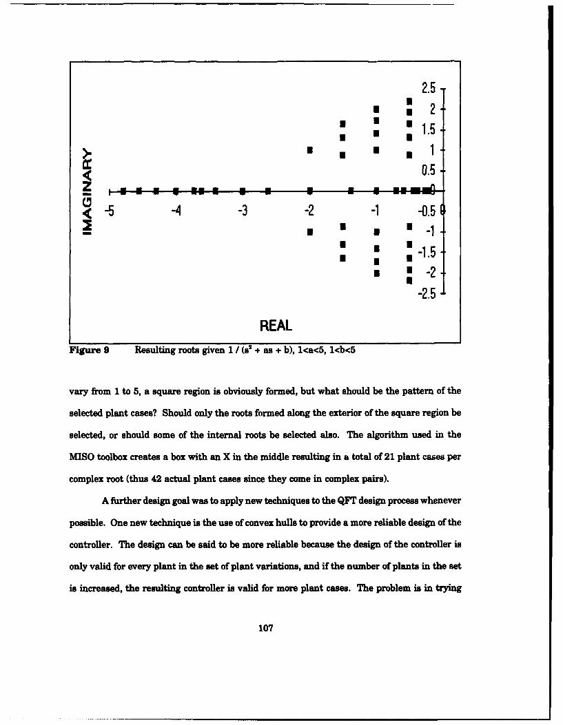
2.5* :2
* 1.5
0.5
< - -3 -2 -1 -0.5
• •.5 -1.
* : * -2-2.5
REALFigure 9 Resulting roots given 1 /W( + as + b), 1<a<5, 1<b<5
vary from 1 to 5, a square region is obviously formed, but what should be the pattern of the
selected plant cases? Should only the roots formed along the exterior of the square region be
selected, or should some of the internal roots be selected also. The algorithm used in the
MISO toolbox creates a box with an X in the middle resulting in a total of 21 plant cases per
complex root (thus 42 actual plant cases since they come in complex pairs).
A further design goal was to apply new techniques to the QFT design process whenever
possible. One new technique is the use of convex hulls to provide a more reliable design of the
controller. The design can be said to be more reliable because the design of the controller is
only valid for every plant in the set of plant variations, and if the number of plants in the set
is increased, the resulting controller is valid for more plant cases. The problem is in trying
107
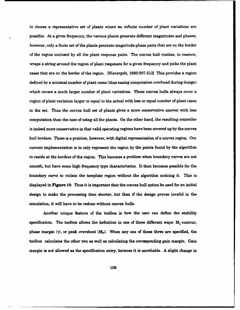
to choose a representative set of plants where an infinite number of plant variations are
possible. At a given frequency, the various plants generate different magnitudes and phases;
however, only a finite set of the plants generate magnitude-phase pairs that are on the border
of the region enclosed by all the plant response pairs. The convex hull routine, in essence,
wraps a string around the region of plant responses for a given frequency and picks the plant
cases that are on the border of the region. [Nievergelt, 1993:307-313] This provides a region
defined by a minimal number of plant cases (thus easing computation overhead during design)
which covers a much larger number of plant variations. These convex hulls always cover a
region of plant variation larger or equal to the actual with less or equal number of plant cases
in the set. Thus the convex hull set of plants gives a more conservative answer with less
computation than the case of using all the plants. On the other hand, the resulting controller
is indeed more conservative in that valid operating regions have been covered up by the convex
hull borders. These is a problem, however, with digital representation of a convex region. Our
current implementation is to only represent the region by the points found by the algorithm
to reside at the borders of the region. This becomes a problem when boundary curves are not
smooth, but have some high frequency type characteristics. It then becomes possible for the
boundary curve to violate the template region without the algorithm noticing it. This is
displayed in Figure 10. Thus it is important that the convex hull option be used for an initial
design to make the processing time shorter, but then if the design proves invalid in the
simulation, it will have to be redone without convex hulls.
Another unique feature of the toolbox is how the user can define the stability
specification. The toolbox allows the definition in one of three different ways: ML-contour,
phase margin (y), or peak overshoot (Mp). When any one of these three are specified, the
toolbox calculates the other two as well as calculating the corresponding gain margin. Gain
margin is not allowed as the specification entry, because it is unreliable. A slight change in
108
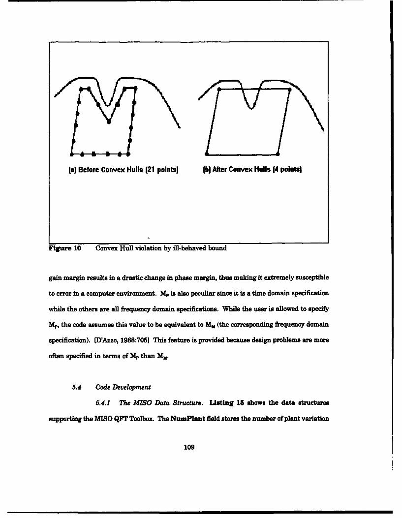
(a) Before Convex Hulls (21 points) (b) After Convex Hulls (4 points)
Figure 10 Convex Hull violation by ill-behaved bound
gain margin results in a drastic change in phase margin, thus making it extremely susceptible
to error in a computer environment. Me is also peculiar since it is a time domain specification
while the others are all frequency domain specifications. While the user is allowed to specify
Me, the code assumes this value to be equivalent to M. (the corresponding frequency domain
specification). [D'Azzo, 1988:7051 This feature is provided because design problems are more
often specified in terms of Mp than MM.
5.4 Code Development
5.4.1 The MISO Data Structure. Listing 15 shows the data structures
supporting the MISO QFT Toolbox. The NumPlant field stores the number of plant variation
109
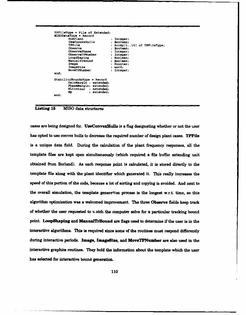
TPFileType = File of Extended;MISODataType = Record
NumPlant Integer;UseConvexHulls .Boolean;TPFile Array[l..16] of TPFileType;Observe Boolean;ObservePhase Integer;ObserveTPNumber Integer;LoopShaping : Boolean;ManualTrBound Boolean;Image . Pointer;ImageSize . word;MoveTPNumber . Integer;
end;
StabilityBoundsType = RecordGainMargin : extended;PhaseMargin: extended;MLContour extended;MP : extended;
end;
Listing 15 MISO data structures
cases are being designed for. UseConvexHulls is a flag designating whether or not the user
has opted to use convex hulls to decrease the required number of design plant cases. TPFile
is a unique data field. During the calculation of the plant frequency responses, all the
template files are kept open simultaneously (which required a fie buffer extending unit
obtained from Borland). As each response point is calculated, it is stored directly to the
template file along with the plant identifier which generated it. This really increases the
speed of this portion of the code, because a lot of sorting and copying is avoided. And next to
the overall simulation, the template genere.ion process is the longest w.r.t. time, so this
algorithm optimization was a welcomed improvement. The three Observe fields keep track
of whether the user requested to watch the computer solve for a particular tracking bound
point. LoopShaping and ManualTrBound are flags used to determine if the user is in the
interactive algorithms. This is required since some of the routines must respond differently
during interactive periods. Image, ImageSize, and MoveTPNumber are also used in the
interactive graphics routines. They hold the information about the template which the user
has selected for interactive bound generation.
110

The StabilityBoundsType record is used to hold the stability specifications. It is self
explanatory from its field names.
5.4.2 The MISO Object. The MISO Object itself really consists of little more
than the support for the menubar. Its only job is to act as the go-between for the user and its
constituent objects. There are six of these constituent objects within MISO: QBounds,
QSpecPla, QDistTem, QFilter, QLoopSha, and QSimulat. Essentially, there is one object per
main menu noun. Each object contains the methods to handle each of the verbs in their
respective pull down menu. These objects have not be,, decomposed into actors; however,
MISO does use the Control object concept as discussed in Section 4.4.4.6.
5.5 User Interface Development
5.5.1 The MISO Menu Structure. Figure 11 shows the desktop for the MISO
QFT toolbox. The menu command words are all nouns and are listed in chronological design
order. Beyond that, the menuing system design is identical to that of the main ICECAP-PC
package.
5.5.2 Interactive Graphics.
5.5.2.1 Loop shaping. There are three overall approaches to
loop shaping within a CAD package: (1) manual, (2) interactive, and (3) automatic. Manual
loop shaping has been implemented. Manual loop shaping requires the student to leave the
MISO toolbox, and use ICECAP-PC to build an L. that meets the tracking and boundary
restraints. When the Lo transfer function has been found, the student returns to the MISO
toolbox and enters that L. directly. Interactive loop shaping provides the student with ar
iterative loop of entering poles and zeros and seeing the resulting graph with the tracking and
111
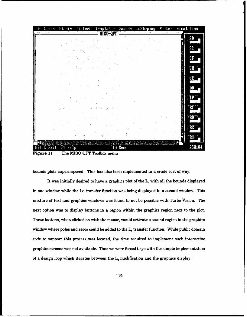
"ISO-QFT
Figure 11 The MISO QFT Toolbox menu
bounds plots superimposed. This has also been implemented in a crude sort of way.
It was initially desired to have a graphics plot of the Lo with all the bounds displayed
in one window while the Lo transfer function was being displayed in a second window. This
mixture of text and graphics windows was found to not be possible with Turbo Vision. The
next option was to display buttons in a region within the graphics region next to the plot.
These buttons, when clicked on with the mouse, would activate a second region in the graphics
window where poles and zeros could be added to the Lo transfer function. While public domain
code to support this process was located, the time required to implement such interactive
graphics screens was not available. Thus we were forced to go with the simple implementation
of a design loop which iterates between the L. modification and the graphics display.
112
The fully automated construction of an L. was also not implemented due to the same
time constraints. The implementation, however, would be a straight forward port of Dr
Thompson's linear programming code. [Thompson, 1990]
5.5.2.2 Bound Generation. The same issues associated with
interactive graphics screens for the loop shaping routines apply to bound generation. However,
more progress has been made with the bound generation interaction than with the loop
shaping due to the simplicity of the bound generation task. The user can choose to interact
with the tracking bound generation routines in two ways. First, they can watch the computer
display textual listings of the calculations it is making for a particular template for a
particular bound point. Or secondly, they can choose to move a plant template around on the
L. graphics screen using the cursor keys. The screen displays several pertinent position values
as the template moves around. When the user finds a position of the template that matches
the 8R value for that template at that phase, they press the INSERT key to mark a point on
the screen representing a point on the tracking bound. When they finish marking a collection
of points, they are saved to the same file which the computer would have generated
automatically if automatic generation had been selected.
5.6 Summary
This chapter appears short compared to the previous chapter while the work done was
the bulk of the thesis effort. This is misleading. In order to make this thesis body less
cluttered and more modular-much like the code-the bulk of this chapter is really contained
within Appendix E.
Section 5.1 presented the options available in implementing the toolbox concept.
Section 5.2 introduced the MISO QFT Toolbox design. Section 5.3 highlighted wine of the
113
more pertinent design decisions made during the MISO process implementation. Section
5.4.1 discussed the design of the MISO data structure. Section 5.4.2 presented the MISO
object design. Section 5.5.1 detailed the design of the MISO user interface. Finally, Section
5.5.2 presented the implementation of interactive graphics routines within the bound
generation and loop shaping functions.
114
6 Testing and Validation
This chapter covers the testing and validation of numerical algorithms used in
ICECAP-PC as well as the correct operation of the user interface. It does not contain code
certification tests because the Turbo-Pascal integrated environment contains several excellent
debugging tools including the ability to allocate and de-allocate break points on the fly, the
ability to monitor and change variable values during program execution, and a watch window
where the software engineer can watch a complete range of variables while single stepping
through the code. Virtually all code used in this project was validated using this environment
and very little was left in the way of script files, text reports, etc.
We did perform extensive testing on algorithms to ensure the best possible numerical
accuracy. It was impossible to include all these tests; therefore, this chapter contains a
representative sample.
6.1 Black Box Testing
Black box testing treats a program as a black box that accepts an input, operates on
it, and generates an output. Using a large test set of previously solved exemplars, a program
can be validated to work over a large range of problems. Text books proved to be a source for
examples, but not the best source for examples. Text books tend to have problems worked on
dated software packages that may not have the numerical precision of ICECAP-PC. A better
source tends to be MATRIXx and MATLAB. The best source, of course, are problems worked
by hand.
An important group of black box problems is to use zero transfer functions or zero
matrices, etc. These examples oftea uncover divide by zero errors and floating point overflows.
Another important group of exemplars were those for the transfer function, polynomial,
or matrix definition lines. Different users input the item definition in different ways. Spaces
115
are put in different places, commas are used instead of spaces, complex conjugate pairs may
both be entered or not, the complex letter could be put either before or after the sign of the
complex value (i.e., 2 -j2 or 2 j-2), etc. The effort was made to keep as few rules as possible
placed on the user. To do this, there was required a large number of exemplars to try to cover
every foreseeable type of user input.
6.2 Macro File Object
The purpose of the macro files is to store all of the black box example pages for easy
rerun after any significant change to the ICECAP-PC package. The same examples can be
used for tutorial purposes by new users to watch the ICECAP-PC commands in execution. The
macro file object operates on a simple principle: it replicates the keystrokes the user would
use. The macro files consist of a single keystroke per line. The macro object simply reads the
line and enters the keystroke directly into ICECAP-PC's GetEvent method simulating the
human keyboard input. There are also special commands for inserting comments and pauses
and end of file.
Later work could easily add a macro recording function to allow users to record
keystroke sequences into a macro file for later rerun. This would be easy to implement by just
reversing the code in the macro object.
The difficulty of creating the macro object was in determining what event codes were
generated when the user pressed a key. The Event.What field is equal to evKeyDown. The
Event.KeyCode field is equal to a HEX value unique for each character. The Event.CharCode
is equal to the ASCII character for the key. The Event.ScanCode is equal to a HEX value
unique for each key. ALT and CTRL key combinations follow the same rules. Some special
keys like the ENTER or ALT key combinations also have unique settings for the Event.Buttons
field and the Event.Command field.
116
If not for the IDE, it would have been impractical to trap these events during runtime
and examine their content. A single keystroke can generate several separate events (updating
screen colors, updating what is displayed, internal flags, etc), so several conditions must be
checked on the trap you set. However, once every possible keystroke was trapped and the
event record examined, it was easy to recreate the keystroke from within a macro file.
6.3 White Box Testing
White box testing is like black box testing, but it does not ignore the internal code
implementation of the algorithm. To do white box testing, an example must be constructed
to test every decision point in the code. If it were not for the IDE, this task would have been
insurmountable to test a package as large as ICECAP-PC. However, with the IDE each
routine could be single stepped through while watching a window showing all the variables.
This is the single greatest contributor to the reliability of the new ICECAP-PC code. "Playing
computer" by watching the state transitions of the data allowed us to not only completely
debug our code but also to create better algorithms more suitable to a computer
implementation. By watching all the variables, you become aware of which very large
numbers are being added to very small ones, which variables are being divided by variables
very close to zero, etz.
The highest contributor to the unreliability of the old ICECAP-PC code was that it
used too much memory to run within the IDE. Its only white box testing was accomplished
using print statements inside the code to dump variable values now and then. The IDE is
infinitely more powerful than this antiquated method of white box testing.
Another error in the old ICECAP-PC not found in the new ICECAP-PC due to
advanced white box testing is the opening of files which are never closed. In the new ICECAP-
PC, only two object methods open, access, and close any file. One method writes to the file and
117
one method reads from the file. An example is that GetTF and StoreTF are the only two
places in ICECAP-PC where the transfer function data file is ever accessed.
Another error discovered in the old ICECAP-PC by white box testing not to be found
in the new ICECAP-PC is passing parameters to procedures in the wrong order. First, the
object-oriented nature of the new code made procedures more single-input, single-output in
nature so much of this problem was relieved. But for the procedures that still required large
amounts of data transfer, global records were used, as discussed in Section. An example of
this would be the frequency response procedure calling the graphics display procedure. Much
data must be passed between the two for proper operation. The old approach would have been
for the frequency response procedure to pass its variable names to the graphics display
procedure's equivalents. With our new approach, the frequency response procedure has a
global record called FreqData, and the graphics display procedure has a global record called
PlotData. There also exists a third procedure called Freq2PlotRecord which translates the
FreqData variables into the PlotData equivalents. Thus, instead of passing a large number
of parameters, the controlling routine simply makes three procedure calls: the call to the
frequency response, a call to Freq2PlotRecord, and the call to the graphics display. This
method offers several practical advantages beyond the solution of the white box testing errors.
It keeps fewer routines in memory at one time, it allows for more complex algorithms or
manipulations to be performed on the data between the frequency response and the plot
routine than a simple parameter passing, and it provides memory savings by moving the
variables from local storage to global pointer variable records. Furthermore, when you read
the code, each variable becomes very obvious who has authority over its contents since its
owners name is part of its name, i.e., FreqDat^.MinFreqValue.
The third major white box testing error uncovered in the old code was testing on a real
type variable against exact zero, i.e., if x - 0.0 then do something. It is obvious to
118
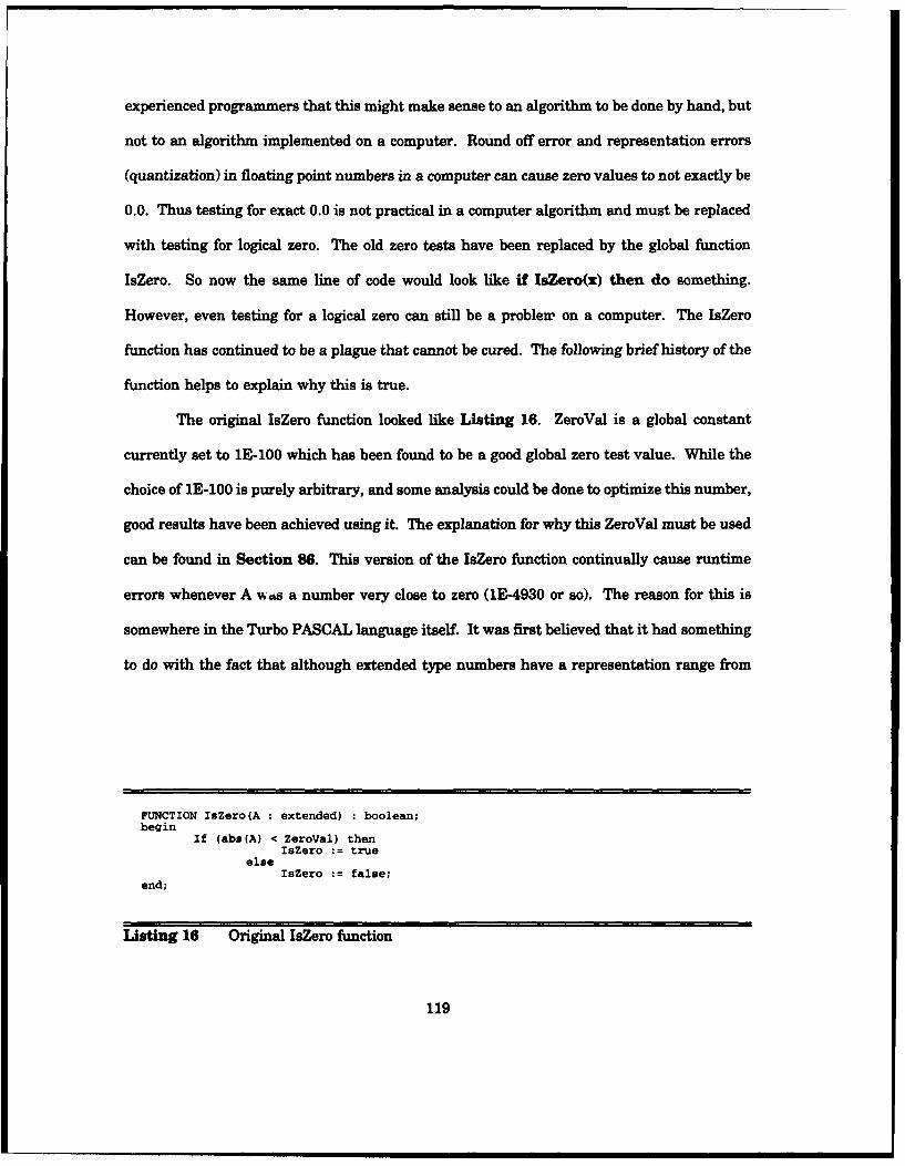
experienced programmers that this might make sense to an algorithm to be done by hand, but
not to an algorithm implemented on a computer. Round off error and representation errors
(quantization) in floating point numbers in a computer can cause zero values to not exactly be
0.0. Thus testing for exact 0.0 is not practical in a computer algorithm and must be replaced
with testing for logical zero. The old zero tests have been replaced by the global function
IsZero. So now the same line of code would look like if IsZero(x) then do something.
However, even testing for a logical zero can still be a problew on a computer. The IsZero
function has continued to be a plague that cannot be cured. The following brief history of the
function helps to explain why this is true.
The original IsZero function looked like Listing 16. ZeroVal is a global constant
currently set to 1E-100 which has been found to be a good global zero test value. While the
choice of 1E-100 is purely arbitrary, and some analysis could be done to optimize this number,
good results have been achieved using it. The explanation for why this ZeroVal must be used
can be found in Section 86. This version of the IsZero function continually cause runtime
errors whenever A as a number very close to zero (1E-4930 or so). The reason for this is
somewhere in the Turbo PASCAL language itself. It was first believed that it had something
to do with the fact that although extended type numbers have a representation range from
FUNCTION IsZero(A : extended) : boolean;begin
If (abs(A) < ZeroVal) thenIsZero true
elseIsZero false;
end;
Listing 16 Original IsZero function
119
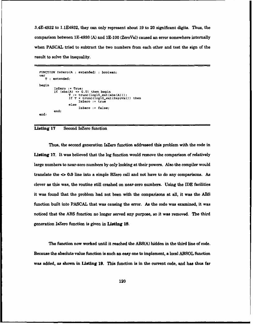
3.4E-4932 to 1.1E4932, they can only represent about 19 to 20 significant digits. Thus, the
comparison between 1E-4930 (A) and 1E-100 (ZeroVal) caused an error somewhere internally
when PASCAL tried to subtract the two numbers from each other and test the sign of the
result to solve the inequality.
FUNCTION IsZero(A : extended) : boolean;var
T extended;
beginIsZero := True;If (abs(A) <> 0.0) then begin
T := trunc(logl0_ext(abs(A)));If T < trunc(loglOext(ZeroVal)) then
IsZero trueelse
IsZero false;end;
end;
Listing 17 Second IsZero function
Thus, the second generation IsZero function addressed this problem with the code in
Listing 17. It was believed that the log function would remove the comparison of relatively
large numbers to near-zero numbers by only looking at their powers. Also the compiler would
translate the <> 0.0 line into a simple BZero call and not have to do any comparisons. As
clever as this was, the routine still crashed on near-zero numbers. Using the IDE facilities
it was found that the problem had not been with the comparisons at all, it was the ABS
function built into PASCAL that was causing the error. As the code was examined, it was
noticed that the ABS function no longer served any purpose, so it was removed. The third
generation IsZero function is given in Listing 18.
The function now worked until it reached the ABS(A) hidden in the third line of code.
Because the absolute value function is such an easy one to implement, a local ABSOL function
was added, as shown in Listing 19. This function is in the current code, and has thus far
120
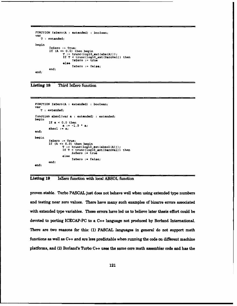
FUNCTION IsZero(A : extended) : boolean;var
T extended;
beginIsZero := True;If (A <> 0.0) then begin
T := trunc(logl0_ext(abs(A)));If T < trunc(loglOext(ZeroVal)) then
IaZero trueelse
IsZero false;end;
end;
Listing 18 Third IsZero function
FUNCTION IsZero(A : extended) : boolean;var
T : extended;
function absol(var a : extended) extended;begin
If a < 0.0 thena := -1.0 * a;
absol := a;end;
beginIsZero := True;If (A <> 0.0) then begin
T := trunc(logl0_ext(absol(A)));If T < trunc(loglO0ext(ZeroVal)) then
IsZero trueelse
IsZero false;end;
end;
Listing 19 IsZero function with local ABSOL function
proven stable. Turbo PASCAL just does not behave well when using extended type numbers
and testing near zero values. There have many such examples of bizarre errors associated
with extended type variables. These errors have led us to believe later thesis effort could be
devoted to porting ICECAP-PC to a C++ language not produced by Borland International.
There are two reasons for this: (1) PASCAL languages in general do not support math
functions as well as C++ and are less predictable when running the code on different machine
platforms, and (2) Borland's Turbo C++ uses the same core math assembler code and has the
121
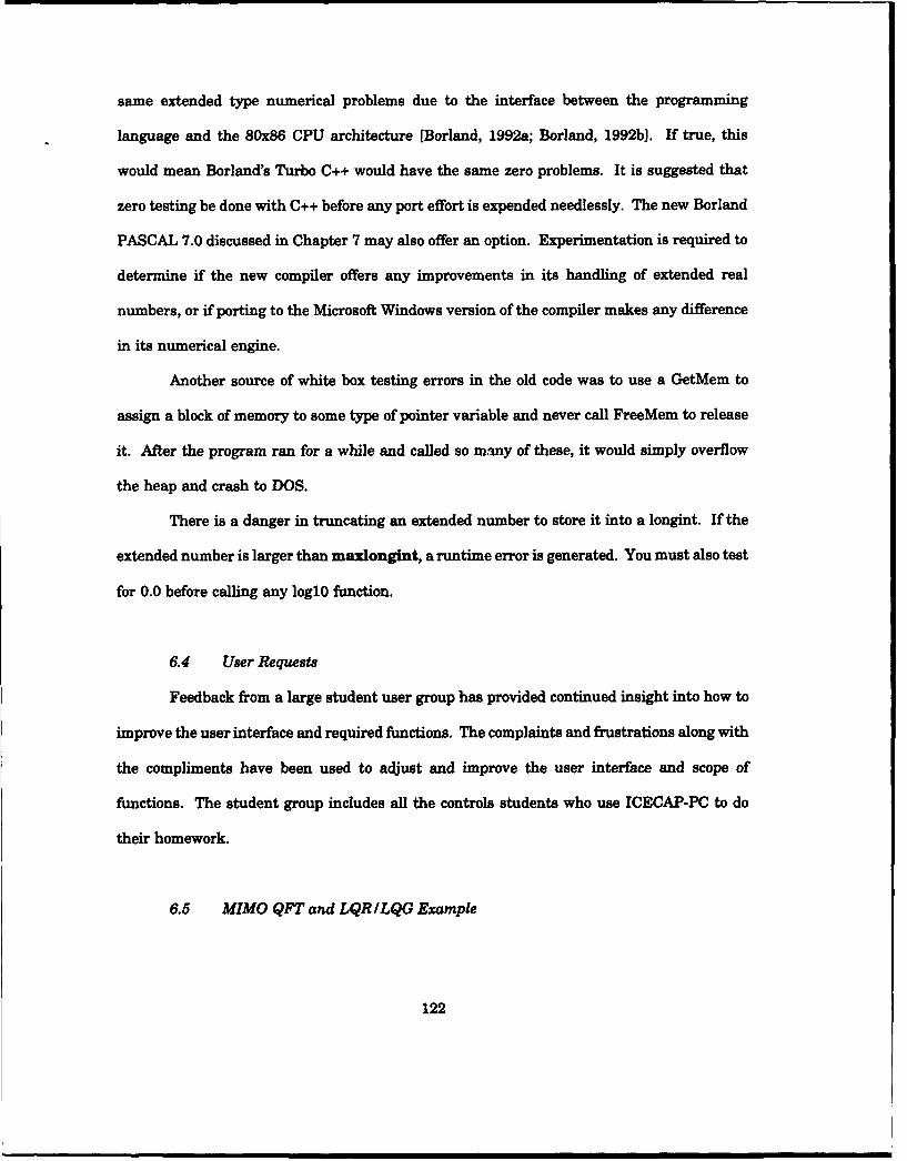
same extended type numerical problems due to the interface between the programming
language and the 80x86 CPU architecture [Borland, 1992a; Borland, 1992b]. If true, this
would mean Borland's Turbo C++ would have the same zero problems. It is suggested that
zero testing be done with C++ before any port effort is expended needlessly. The new Borland
PASCAL 7.0 discussed in Chapter 7 may also offer an option. Experimentation is required to
determine if the new compiler offers any improvements in its handling of extended real
numbers, or if porting to the Microsoft Windows version of the compiler makes any difference
in its numerical engine.
Another source of white box testing errors in the old code was to use a GetMem to
assign a block of memory to some type of pointer variable and never call FreeMem to release
it. After the program ran for a while and called so many of these, it would simply overflow
the heap and crash to DOS.
There is a danger in truncating an extended number to store it into a longint. If the
extended number is larger than maxIongint, a runtime error is generated. You must also test
for 0.0 before calling any logl0 function.
6.4 User Requests
Feedback from a large student user group has provided continued insight into how to
improve the user interface and required functions. The complaints and frustrations along with
the compliments have been used to adjust and improve the user interface and scope of
functions. The student group includes all the controls students who use ICECAP-PC to do
their homework.
6.5 MIMO QFT and LQR/LQG Example
122

A full MIMO 3x3 S-domain (PCT) problem was worked from beginning to end by hand
and by using ICECAP-PC 10.0 to validate its results and to gain insight in both its user
interface and missing capabilities. The example chosen was taken from a 1989 AFIT thesis
by Capt David Bossert. [Bossert, 19891 The same problem was also solved using LQR/LQG
by hand and by using MATRIXx to try to gain insight on the advantages or disadvantages of
other modern control techniques versus QFT as well as commercial CACSD packages versus
ICECAP-PC. Of course, working a MIMO problem not only validates the MIMO toolbox, but
the MISO toolbox as well, along with the core ICECAP package, since each of these pieces are
needed to solve a MIMO problem.
Capt Bossert used ICECAP to design the system and validated his solutions using
Macsyma to simulate the controlled system. The differences between his results and ours can
be explained by his use of pole cancellation assumptions. He was using an older version of
ICECAP which only supported transfer functions of order 10 or less. Therefore, to keep his
intermediates from growing too large during the matrix inversions, he had to manually cancel
some pole-zero pairs that would not otherwise have been cancelled.
6.6 The Root Finder
Appendix B shows listings of our tests comparing ICECAP-PC's root finder with that
of PC-Matlab. In all cases we exceed the accuracy attained in Matlab, often by several decimal
places. However, in the process we noticed something that forced us to modify our algorithm.
The ICECAP-PC root finder first calls the Laguerre method [Vetterling, 1985] to make the
initial cut at the roots. The Laguerre method returns a set of values whose error with the
actual roots is symmetrical with the actual roots in the case of root multiplicity. Hence
coefficient reconstruction is extremely accurate after root finding with the Laguerre algorithm.
The second step used by the ICECAP-PC root finder is the polishing of the rough roots with
123
either the Bairstow method [Vetterling, 19851 in the case of real pairs or with Brents method
[Vetterling, 19851 in the case of single real roots or high root multiplicity. We were able to
achieve extremely accurate roots with these two polishing methods. Improvements of 4-5
decimal places over Laguerre's method was common. However this added accuracy came at
a loss of error symmetry about the actual values. Polynomial coefficient reconstruction is often
degraded with the better roots found by the polishing methods! We finally modified our
algorithm as follows.
We modified the root finder to take the first cut using Laguerre, store the Laguerre
roots, take the second cut using Bairstow and Brent, and store the polished roots, reconstruct
the polynomial coefficients with the Laguerre roots and find a reconstruction error, reconstruct
the polynomial coefficients with the polished roots and find the polished reconstruction error,
and compare the two errors taking the root set yielding the least reconstruction error. Very
often ICECAP-PC settles on the less accurate set of roots because the coefficient reconstruction
error is minimized.
6.7 Summary
While much work has been done to validate the ICECAP-PC 10 code, much work
remains. Code validation is a process which never ends for the life of the program. Each time
the code is examined and each time a new problem example is solved using the package,
improvements and enhancements are made. No computer program is ever fully verified. No
matter how many thesis students offer their experience to the evolution of ICECAP-PC, there
will always be Achilles' heels in the algorithms--one more example that the algorithms cannot
solve or one more error that has been overlooked. However, if constant application of the
validation tools discussed in this chapter is maintained, ICECAP-PC will remain a stable
platform in which to design control systems.
124
In Section 6.1 the black box testing validation tool was discussed. In Section 6.2 we
described how the macro file object is used to support black box testing. In Section 6.3 we
explained the use of the IDE for white box testing and how this testing turned up problems
with the older version of ICECAP-PC. In Section 6.4 the feedback received from the local
AFIT controls student users group was discussed. Section 6.5 discussed the large design
problem used to validate both QFT toolboxes as well as the core ICECAP-PC package and how
these results were compared to the results obtained from using LQR/LQG on Matrixx. Finally,
validation of the root finder was discussed in Section 6.6 and compared to results obtained
from PC-MATLAB.
125
7 Conclusions and Recommendations
7.1 Conclusions
The purpose of this research project was the development of a CACSD program to meet
the needs of an ever more sophisticated educational system. In a day when computer analysis
and simulation pl ys an increasingly important role, control systems engineers need a solid
grasp of the computer sciences. This project exercises the disciplines required by today's
control systems engineer: mathematical rigor, numerical analysis proficiency, advanced OOP
skills, human interface engineering, and control systems engineering. The end product is a
fast, efficient and accurate program with inherent expansion capability.
Fundamental control systems engineering is, of course, the heart of the ICECAP-PC
program. While engineers of other disciplines will undoubtedly find utility in the basic
ICECAP-PC program, they are in fact directed at the control systems engineer. Both classical
and modem control capabilities are provided in the basic ICECAP-PC program. Furthermore,
the Quantitative Feedback Theory is implemented in both its MISO and MIMO forms. The
addition of interactive bounds generation and interactive L0 development provides an ideal
educational platform for QFT.
Because the object library from Borland Turbo Vision was available for use,
productivity in this thesis effort was much higher than would be typically expected in software
development. The functional version of ICECAP-PC always suffered in the contemporary
human factors engineering area because only so much time could be devoted to menuing
systems, output screen formatting, and context sensitive help screens. Using the
professionally packaged object library of Turbo Vision, the we were able to focus almost
completely on mathematical algorithms and let the commercial package take care of user 1/0.
Because of this, the authors have been able to work on expanding ICECAP-PC's CACSD
toolboxes beyond that which could otherwise have been accomplished. Furthermore, future
126
thesis students will be able to go even farther since the overhead of porting the ICECAP-PC
subroutines into an 00 environment has already been accomplished.
7.1.1 General Objectives. The general objectives of this research effort are
presented in Section 1.3 as the development of an 00 CACSD environment, the refinement
of numerical methods, and the development of a MISO QFT toolbox. Each objective was
achieved. The implementation of the 00 environment is discussed in Chapter- 4. Numerical
analysis, an art often overlooked by engineers, was fundamental to the success of this project.
Virtually every numerical algorithm in ICECAP-PC underwent some form of modification.
Much of this is discussed in Section 4.4. Finally, the implementation of the MISO QFT
toolbox is presented in Chapter 5.
The specific design requirements and specifications for this research effort are
presented in Chapter 8. Each of these specifications were met and are discussed in the
following.
7.1.2 General Traits. The general traits presented in Section 3.1 were
largely accomplished through the use of 00 technology. 00 development and programming,
which involves not only a new code structure but an entirely new logic and modeling process,
is the software development basis of the future. 00 decomposition provides software
reusability, extendibility, and maintenance in a way functional decomposition never could.
This is why virtually all new commercial operating system development is taking place using
object-orientation. The engineering disciplines are late comers to object-orientation and none
of the commercial CACSD packages are built on this paradigm as of yet. In this regard,
ICECAP-PC is now a pioneer in the area of placing a CACSD package in an 00 format.
Certainly, this should draw much attention from outside institutions.
127
7.1.3 Programming Standards. The programming standards discussed in
Section 3.2 were all accomplished. The resulting code is very easy to read and follow, and we
consider it self-documenting.
7.1.4 Mathematical Specifications. The mathematical specifications
presented in Section 3.3 were achieved and discussed throughout Section 4.4 as well as all
of Chapter 6. There is considerable improvement in the numerical accuracy, reliability, and
scope of function of ICECAP-PC 10 vs. ICECAP-PC 9.0. Accuracy and reliability have been
improved by improving and validating the mathematical algorithms within ICECAP-PC as
well as making every internal number representation an extended real type-some algorithms
within 9.0 were still using normal real types. An important example of this is the root finder.
For nonrepeated roots, the new algorithms can find the roots to the accuracy of machine
representation (19-20 significant digits) as opposed to 9.0's ability to find the roots to 8-12
significant digits. The scope of ICECAP-PC's matrix math functions have been greatly
enhanced in order to provide modern technique support for the MIMO toolbox.
7.1.5 Human Interface Specifications. Finally, the user interface
requirements given in Section 3.4 were achieved and discussed in Section 4.5. The menuing
system allows effective access to the ICECAP-PC commands for both the novice and
experienced user. The on-line help is so advanced, it may one day become more valuable than
ICECAP-PC's problem solving functions. The desired data display capabilities of ICECAP-PC
were achieved (except the ability to display multiple graphics windows), but this area needs
further research and development.
The user interface of ICECAP-PC 10 is state-of-the-art and far surpasses that
of all previous ICECAP-PC versions as well as surpassing the interfaces in most commercial
128
CACSD packages. The on-line help facility available within ICECAP-PC is also vastly
improved and as convenient and effective as any available in other CACSD packages. The
ability to just click the right mouse button on anything help is desired on is very effective.
The data presentation part of ICECAP-PC's user interface is currently only average, but with
further development of the interactive graphics routines, they could be superior to any CACSD
package currently available.
At this point, we must emphasize that excellence in all of the above disciplines mean
nothing if the human interface is ignored. In todays business climate, intuitiveness is key
rather than superfluous to software design. An intuitive program is quickly learned saving
expensive engineering time for the actual design process. The adage that "the utility of a
program is inversely proportional to its interface" is absolute nonsense. There are many
excellent 00 interface development tools that remove much of the burden of interface
development such as mouse support, drop down menus, etc. ICECAP-PC uses one such tool,
the Borland Turbo Vision language extension.
The result of exercising the above disciplines is a CACSD program that challenges the
state-of-the-art in CACSD program design in form, in use, and in utility. There is still much
work to be done. However, we laid complete, cohesive foundation paving the way for future
development of ICECAP-PC and broke new ground in applying object-orientation to CACSD
packages.
7.2 Recommendations
ICECAP-PC would be considered in the software industry to be a medium sized
software development project. To a single thesis student, this translates into an
insurmountable task. It was never expected that all our goals for ICECAP-PC would be
129
achieved in an 18-month thesis period. The following paragraphs outline the most important
remaining goals.
7.2.1 Error Handling Routine. There is a need for an object which can trap
all system error interrupts before the program crashes to DOS. The routine could then print
a message to the user describing what has happened, clear all the system flags, and return to
execution.
7.2.2 Database Object. The original data file storage/retrieval system was
at first a single file. Single file in the beginning, but then broke into TFs, POLYs, MATRIX.
There is an extensive need for future thesis effort to address the construction of a
database object. This new object would serve at least two purposes: (1) consolidate all the
data files into one, and (2) serve as a data dictionary for the code development. The same
database object could maintain the two separate databases.
Having a database object that can keep track of the various sets of data has become
more important as the MIMO QFT toolbox has matured. There is both overhead in the code
and user interface for keeping the MISO equivalent session files straight as well as disk
clutter overhead for all the MIMO datafiles. There are also some tricky techniques in the code
to take care of the different transfer function names and filenames between the basic ICECAP-
PC and the MISO QFT toolbox. A global TransFuncFileName variable is used to make the
GetTF and StoreTF, etc procedures global. And a special type of header variable had to be
made global for all the transfer function dialogue boxes to work in both QFT and normal
ICECAP-PC. A database object could be used as an overseeing monitor to keep these types
of differences straight. It would also make the code more purely 00 by representing this
130

database function as an object structure instead of the spread out pieces of functional code we
have patched the problem with.
The importance of a database object is also seen in our lack of a data dictionary for our
code. While a data dictionary is viewed as a traditional part of a large CAD package such as
ICECAP-PC, it was not given a large priority in this thesis effort. We believe we have
replaced the need for a data dictionary by using global records instead of separate global
variables. For example, all the global variables needed to allow any toolbox to use the
graphics object are maintained in the PlotData record. This has some profound advantages
over the old technique of putting all global variables in the global file called ICEDEL.PAS.
First, there is no confusion on what variables must be set before a graphics call; set
each of the variables in the record that pertain to the call about to be made.
Second, the despicable practice of using a global variable for one purpose in one section
of code and then using it for another in a different set of code is eliminated; who would even
think of using PlotData.HorzGraphSize as a counter variable in a frequency response
procedure.
Third, the PlotData record can be made into a pointer variable so that no matter how
large the arrays become inside the record, they are always stored in heap space (640K) instead
of the data segment (64K); this has a profound impact on making the size and number of
toolboxes available to ICECAP-PC virtually unlimited.
Fourth, while the global variables needed for the graphics object, for example, could
be made part of the interface section of the graphics object itself-and perhaps this is the most
purely 00 approach--this is not a practical solution. This would mean that for the frequency
response object to send its response data to the graphics object for plotting, the frequency
object would have to instantiate the graphics object inside itself. It is obvious that the levels
of this object instantiation could become very memory expensive very quickly. By using the
131
global records, only one object must be maintained in memory at any one time along with one
pointer for every object's global data record. Thus, the frequency response object builds its
data variables and then assigns them appropriately into the graphics object's data record.
Then the frequency response object is removed from memory since its job is complete, and the
graphics object is instantiated and signaled to operate its plot method on its global data record.
Finally, if the database object is ever created, the record structure will make the
implementation of the database object almost invisible to the current code.
7.2.3 The Root Finder. The current root finder, crucial to MIMO QFT,
reaches performs at the level of the floating point resolution of the machine. This isn't good
enough. ICECAP-PC should guarantee root finding to 20 significant decimal digits. In order
to do this, calculations must be performed with far greater resolution, say 100-200 decimal
digits. None of the IEEE 754 floating point number definitions provide for this. Therefore,
the root finder must declare its own data structure and operate this way. Defining a new data
structure for a number entails defining all the base mathematical routines such as addition,
subtraction, etc. Several optior 3 are available and should be studies. Consider the following
definitions
In the first example, a number is defined as a record of two extended numbers.
Operations on this type would be very fast, but may lack in other areas. The second example
defines a number as two very large integer arrays and the third defines a number as two
string variables. Each of these definitions could yield advantages and disadvantages and
should be studied for possible use in the root finder.
7.2.4 Multiple Windows. Future thesis work should build multi-windowed
displays which allow the student to view several different types of plots at one time for the
132
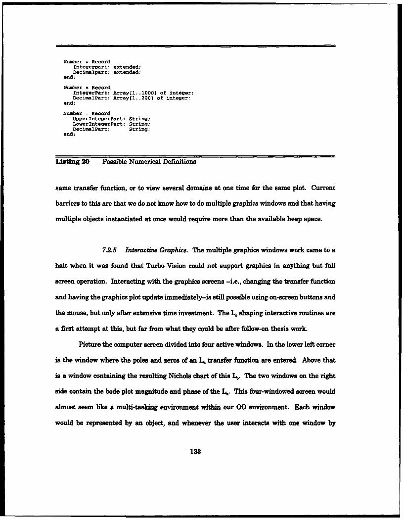
Number = RecordIntegerpart: extended;Decimalpart: extended;
end;
Number = RecordIntegerPart: Array[l..1000] of integer;DecimalPart: Array[1..200] of integer;
end;
Number = RecordUpperlntegerPart: String;LowerlntegerPart: String;DecimalPart: String;
end;
Listing 20 Possible Numerical Definitions
same transfer function, or to view several domains at one time for the same plot. Current
barriers to this are that we do not know how to do multiple graphics windows and that having
multiple objects instantiated at once would require more than the available heap space.
7.2.5 Interactive Graphics. The multiple graphics windows work came to a
halt when it was found that Turbo Vision could not support graphics in anything but full
screen operation. Interacting with the graphics screens -i.e., changing the transfer function
and having the graphics plot update immediately-is still possible using on-screen buttons and
the mouse, but only after extensive time investment. The L4 shaping interactive routines are
a first attempt at this, but far from what they could be after follow-on thesis work.
Picture the computer screen divided into four active windows. In the lower left corner
is the window where the poles and zeros of an L4 transfer function are entered. Above that
is a window containing the resulting Nichols chart of this L4. The two windows on the right
side contain the bode plot magnitude and phase of the L4. This four-windowed screen would
almost seem like a multi-tasking environment within our 00 environment. Each window
would be represented by an object, and whenever the user interacts with one window by
133
creating an event, each object would receive the event message. Each object would react to
the events. If the user selects the lower left window area and modifies a pole or zero, that
windows event would react by redrawing the transfer function. The other three objects would
also react by redrawing the graphs in their windows for the new transfer function.
7.2.6 Interactive Tracking Specification Generation. Currently the QFT
Toolbox requires TRu and TRL to be designed off-line by the user and entered manually. The
design of these specification transfer functions is crucial to a successful QFT design, and an
educational package like ICECAP-PC should include a tutorial type environment to assist the
user in constructing these transfer functions. Valuable insights into their construction could
be offered through the help facilities during their design. One example of the kind of help
that should be made available is a simultaneous display of 8R so the user can readily see if
the current TRu and TRL transfer functions provide a 8 R which is monotonically increasing for
all frequencies. Another example would be some text screens of the engineering wisdom of the
AFIT staff. For example, a recent situation arose where the figure of merit specifications on
TRu and TRL were such that an all-real-pole transfer function would not work. [Houpis, 1992b]
A complex pair of poles was added near a real pole to provide a response which had a quicker
rise time, but no overshoot. This type of engineering insight would be an invaluable addition
to every help screen for every function within ICECAP-PC. Indeed, if ICECAP-PC's help
facilities became a depository for engineering experience and rules of thumb, the value of the
help screens would quickly surpass the value of the package for educational purposes.
7.2.7 Augmented Model Bound Generation. As discussed in the QFT Users
Manual, it is important that TRu and TRL be designed so that 6R is monotonically increasing
for all frequencies. It is suggested that at the highest frequency of performance concern, a zero
134
be added to TRU and a pole be added to TRL to avoid problems at high frequencies. Later work
on ICECAP-PC should add an AUGMENT MODEL command which does this for the user who
may not have known to do it in the initial design of TRu and TRL.
The MISO QFT toolbox needs to allow the user to adjust the BI and Bu tracking
responses to account for disturbance from cross terms in a MIMO design. [Sating, 1992] The
new code would simply need to allow the user to modify the listing of values for 8. to make
them more strict--smaller. The tracking bounds would then be generated using the new values
of8.
Another technique for augmenting the model was discovered during a telephone
conversation with Capt David Bossert [Bossert, 19921. He is currently researching a way to
implement an upper bound on the magnitude of L. at each design frequency to account for
device saturation. He cites examples in his work where the large error gains associated with
QFT design saturate actuators in systems for which he designs QFT controllers. These bounds
would be used as upper bounds on the traditional composite bounds. ICECAP-PC should add
a capability in the composite bound generation and in the loop shaping algorithms to account
for this.
7.2.8 Interface to Commercial Packages. Because commercial packages offer
such a wide variety of specific techniques, ICECAP-PC will never be able to offer all of them.
Perhaps the largest lacking function is an ability to do state-time simulations. Because all of
these functions cannot be offered directly, an ability to generate information in ICECAP-PC
and then port this information to the other packages is desirable. Porting information in the
reverse direction is also important. One might want to construct a very large system using
Matrixx's System Build facilities and then input this information into ICECAP-PC in the form
of matrices or transfer functions. ASCII formatted data files appear to be the standard media
135
of choice for most popular commercial CACSD packages. The problem is not in generating a
properly formatted file in ICECAP-PC or reading a file into ICECAP-PC, the problem is in
obtaining the file format for each commercial package. ICECAP-PC has the required
functionality, what is now required is development time to build the required file formats.
7.2.9 System Build Toolbox. We believe a crude but effective system build
type function could be easily constructed using the type of dialog box built for the FORM CLTF
option. Many possible systems can be built from the one dialogue box. Several different basic
types of dialogue boxes could be made available for hundreds of possible systems. The
possibilities could grow exponentially if some of the dialogue boxes included other dialogue
boxes as one of their element choices.
7.2.10 Discrete Toolboxes. Considerably more time was required in porting
ICECAP-PC 9.0 to the 00 ICECAP-PC 10 than was originally expected. This resulted in an
incomplete incorporation of the discrete domain capabilities. Some of the work has been done,
and more will be completed during the weeks after this thesis period ends, but work wil!
remain for following thesis students.
7.2.11 Nonlinear Toolbox. A nonlinear toolbox is a larger task than most of
the others listed here. The basic idea is to provide the user with an interactive environment
in which to model nonlinearities as linear functions. The user then compares the time and
frequency response characteristics of the model to those of nonlinear system and iterates the
model design until the datums match within specifications.
136
7.2.12 Time Delay Toolbox. In order to solve the large class of problems which
contain time delay elements, a time delay toolbox will need to be added to ICECAP-PC. This
toolbox must handle time delays in both the time and frequency domains, both discrete and
continuous. The transfer function routines must be augmented to allow the entry of a time
delay symbol during transfer function definition.
7.2.13 Transcendental Functions Toolbox. There is a need for a screen to
provide transfer function approximations to transcendental functions. For example, if a
student has a transfer function with e" which cannot be entered directly into the transfer
function definition, he could enter the approximation screen and generate a pole-zero
combination to approximate that function over some range. Possible functions would be the
exponential, sine, and cosine.
7.2.14 Borland PASCAL 7.0. In the final weeks of this thesis period, Borland
shipped the upgrade to Turbo PASCAL 6.0 as well as a new Turbo Vision. This new version
provides some startling breakthroughs. The 640K memory barrier for personal computers is
eliminated with a new DOS Protected Mode Interface (DPMI) driver which has been released
to public access. This results in increased speed for ICECAP-PC since the use of overlay files
are no longer needed. It also results in higher order problems and higher resolution listings
and plots. The new Integrated Development Environment (IDE) further expands its CASE-like
features. Also new compilers and dialog box builders allow ICECAP-PC to be easily ported to
the Microsoft Windows environment, if desired. Finally, if the user has a '386 or '486 machine,
the new compiler allows mathematical enhancement instructions which can increase math
performance up to five times. The disadvantage of the new PASCAL is that it no longer
supports XT machines, at least a '286 processor is required.
137
7.3 Summary
In summary of both Chapter 7 and the research paper as a whole, the author must
emphasize his enthusiasm for what has been achieved with ICECAP-PC 10. AFIT has had a
long and proud tradition of producing state-of-the-art CACSD packages for the public domain.
TOTAL was the first at AFIT and the first in the world. ICECAP-PC 10 is also a first in the
world: the first 00 CACSD package for the public domain. Its 00 user interface has no equal
both for beginning users who need extra help and for the advanced users who want direct
access to the functions they need. The full screen editor and the log file options ICECAP-PC
now provides allow the student to produce extremely readable output reports to hand in with
their homework. The elegance of the 00 code and the extensive white and black box testing
accomplished provide protection against both runtime errors and unreliable answers. By far,
ICECAP-PC 10 is the best choice for students and professors alike in their choice for CACSD
software to use for class and thesis work.
138
Appendices

Appendix A Bibliography
Appendix A: Bibliography
Ash, Raymond H. and Gerald R. Ash. "Numerical Computation of Root Loci Using theNewton-Raphson Technique," IEEE Transactions on Automatic Control. 376-382. October1968.
Bailey, F. N. and others. "The Loop Gain-Phase Shaping Design Programs," QuantitativeFeedback Theory Symposium Proceedings WL-TR-92-3063. 565-574. Wright-Patterson AirForce Base OH: Wright Laboratory (ASD), August 1992.
Ballance, D. J. and P. J. Gawthrop. "QFT, the UHB, and the Choice of the TemplateNominal Point," Quantitative Feedback Theory Symposium Proceedings WL-TR-92-3063.74-79. Wright-Patterson Air Force Base OH: Wright Laboratory (ASD), August 1992.
Barker, H. A. "User Interface Standards for Control System Design Applications," 1989IEEE Control Systems Society Workshop on Computer-Aided Control System Design(CACSD). 86-93. New York: The Institute of Electrical and Electronics Engineers, Inc.,1989.
Borland International, Inc. Tubro Pascal 6.0 Programmers Guide, Scotts Valley, CA:Borland International Inc, undated.
Borland International, Inc. Tubro Pascal 6.0 Turbo Vision Guide, Scotts Valley, CA:Borland International Inc, 1991.
Borland International, Inc. Charlie Clabert on Turbo PASCAL user support hotline.Telephone Interview. 18 November 1992a.
Borland International, Inc. Jacqueline on Turbo C++ user support hotline. TelephoneInterview. 18 November 1992b.
Bossert, David Edward. Design of Pseudo-Continuous Time Quantitative Feedback TheoryRobot Controllers. MS Thesis, AFIT/GE/ENG/89D-2. School of Engineering, Air ForceInstitute of Technology (AU), Wright-Patterson AFB OH, December 1989.
Bossert, David Edward, Captain US Air Force. Telephone Interview. Air Force Academy,13 November 1992.
Burden, Richard L. and Douglas J. Faires. Numerical Analysis. Boston: PWS-KentPublishing Company, 1981.
Chapra Stephen C. and Raymond P. Canale. Numerical Methods for Engineers. New York:McGraw-Hill Book Company, 1988.
Chiang, Richard Y. and Michael G. Safanov. Robust Control Toolbox User's Guide. NatickMA: The Math Works, Inc, 1 June 1988.
Chikofsky, E. J. Software Development: Computer-Aided Software Engineering (CASE).IEEE Computer Society Press Technology Series.
I
Curtis, Bill. "Prototyping Versus Specifying: A Multiproject Experiment," Tutorial:Human Factors in Software Development. pg 298.
DAC Micro Systems. dCOM The Directory Commander. Lancaster CA: DAC MicroSystems, undated.
D'Azzo, John J. and Constaintine H. Houpis. Linear Control System Analysis & Design(Third Edition). New York: McGraw-Hill Book Company, 1988.
Dongarra J. J. Linpack Users Guide. Philadelphia: SIAM, 1979.
Fisher, Jeff and Dale Gipson. "In Search of Elegance," Computer Language, 37-46(November, 1992).
Frederick, D. K. and M. Rimer. "Benchmark Problems for Computer-Aided Control SystemDesign," Computer Aided Design in Control Systems (IFAC 1988). 1988.
Frdberg, Carl_Erik. Numerical Mathematics. Menlo Park: The Benjamin/CummingsPublishing Company, Inc, 1985.
Gerald, Curtis F. Applied Numerical Analysis. Menlo Park: Addison-Wesley PublishingCompany, 1978.
Grace, Andrew. Optimization Toolbox User's Guide. Natick MA: The Math Works, Inc.,November 1990.
Horowitz, Isaac and Clayton Loecher, "Design of a 3x3 multivariable feedback system withlarge plant uncertainty," International Journal of Control, Vol 33 No 4:677-699, 1981.
Houpis, Constaintine. Quantitative Feedback Theory Technique for DesigningMultivariable Control Systems. AFWAL-TR-86-3107. Wright-Patterson AFB OH: AirForce Wright Aeronautical Laboratories, 1987.
Houpis, Constantine H. and Gary B. Lamont. Digital Control Systems: Theory, Hardware,Software (Second Edition). New York: McGraw-Hill, Inc, 1992.
Houpis, Constantine H. AFIT Guidance and Controls Chairman. Personal Interview. AirForce Institute of Technology (AU), Wright-Patterson AFB OH, 13 November 1992b.
Houpis, Constantine H. "List of Quantitative Feedback Theory (QFT) Symbols,"Quantitative Feedback Theory Symposium Proceedings WL-TR-92-3063. 19-24. Wright-Patterson Air Force Base OH: Wright Laboratory (ASD), August 1992c.
IEEE. Binary Floating-Point Arithmetic. IEEE Std 754. New York: IEEE, 1985.
Integrated Systems, Inc. MatrixX User's Guide Version 6.0. Santa Clara CA: IntegratedSystems, Inc, May 1986a.
Integrated Systems, Inc. System._Build User's Guide. Santa Clara CA: IntegratedSystems, Inc, May 1986b.
2
Jones, John. "Stabilization of NonLinear Time-Varying Control Systems," SoutheasternSimulation Conference Proceedings, 1993.
Kheir, Naim. Systems Modeling and Computer Simulation. New York: Marcel DekkerInc., 1988.
Kobylarz, Thomas J. Flight Controller Design with Nonlinear Aerodynamics, LargeParameter Uncertainty and Pilog Compensation. MS Thesis. School of Engineering, AirForce Institute of Technology (AU), Wright-Patterson AFB OH, December 1988.
Kreyszig, Erwin, Advanced Engineering Mathematics (Fifth Edition), New York, JohnWiley & Sons, 1983.
Larimer, Stanley, An Interactive Computer-Aided Design Program for Discrete andContinuous Control System Analysis and Systhesis. MS Thesis. School of Engineering, AirForce Institute of Technology (AU), Wright-Patterson AFB OH, 1978.
Lempp, Peter and Rudolf Lauber. Software Development: Computer-Aided SoftwareEngineering (CASE). IEEE Computer Society Press Technology Series.
Lial, Margaret L. and Charles D. Miller. Algebra and Trigonometry (Second Edition).Dallas: Scott, Foresman and Company, 1980.
MathSoft, Inc. Mathcad 3.0 User's Guide. Cambridge MA. MathSoft Inc, June 1991.
Microsoft Corporation. Microsoft Windows User's Guide. Document No. 620299-00 REV A.Microsoft Corporation, Redmond WA, 1990.
Mashiko, Susan and Gary Tarcjynski. Development of a Computer Aided Design Packagefor Control System Design and Analysis for a Personal Compute. Vol I and II.ADA163940(I), ADA164044(II). MS Thesis, AFIT/ENG/86D8. School of Engineering, AirForce Institute of Technology (AU), Wright-Patterson AFB OH, December 1985.
Moler, Cleve and others. PC-MATLAB for MS-DOS Personal Computers User's GuideVersion 3.2-PC. Sherborn MA: The Math Works, Inc, 8 June 1987.
Moore, Paul A. Extension of the Software Development Workbench to IncludeMicrocomputer Workstations. ADA151903. MS Thesis, AFIT/GCS/ENG/84D-18. Vol I andII. School of Engineering, Air Force Institute of Technology (AU), Wright-Patterson AFBOH, December 1984.
Nievergelt, Jurg and Klaus H. Hinrichs. Algorithms and Data Structures. EnglewoodCliffs, NJ:Prentice Hall. 307-313. 1993.
O'Brian, Fredrick L, Consolidated Computer Program for Control System Design. MSThesis, AFIT/GE/ENG/84D-18. School of Engineering, Air Force Institute of Technology(AU), Wright-Patterson AFB OH, December 1977.
3
Parisi, V.M., Development of a Computer-Aided Design Package for Control System Designand Analysis for Use on a Personal Computer, Vol I and II. ADA138065. MS Thesis, AirForce Institute of Technology, Wright-Patterson AFB, Dayton, OH, December, 1983.
Press, William H. Numerical Recipes: The Art of Scientific Computing London: CambridgeUniversity Press, 1989.
Pressman, Roger S, Software Engineering: A Practitioner's Approach (Second Edition).New York: McGraw-Hill Pub Co, 1987.
Rabinowitz, P. A First Course in Numerical Analysis (Second Edition). New York:McGraw-Hill, 1978.
Ravn, Ole. "On User-Friendly Interface Construction for CACSD Packages," 1989 IEEEControl Systems Society Workshop on Computer-Aided Control System Design (CACSD). pp35-40. New York: The Institute of Electrical and Electronics Engineers, Inc., 1989.
Reid, Gary J. Linear System Fundamentals. New York: McGraw-Hill Book Company,1983.
Rumbaugh, James. Object-Oriented Modeling and Design. Englewood Cliffs: PrenticeHall, 1991.
Sating, Richard R. Development of an Analog MIMO QFT Cad Package. MS Thesis.School of Engineering, Air Force Institute of Technology (AU), Wright-Patterson AFB OH,December 1992.
Smith, Sidney L. and Jane N. Mosier. Guidelines for Designing User Interface Software.ESD-TR-86-278. Contract MTR-10090. Bedford MA: MITRE, August 1986 (AD-A177 198).
Smith. Matrix Eigensystem Routines: EISPACK Guide. Berlin: Springer-Verlag, 1976.
Tannenbaum, Andrew S. Stuctured Computer Organization. Englewood Cliffs: PrenticeHall.
Thompson, D. F. "Optimal and Sub-Optimal Loop Shaping in Quantitative FeedbackTheory," PhD. Thesis, School of Mechanical Engineering, Purdue University, WestLafayette, IN. August, 1990.
Thompson, Peter M. User's Guide to Program CC, Version 3. Contract F33657-83-0242.Hawthorne CA: Systems Technology, Inc., March 1985.
Trevino, Fred. An Object Oriented Computer Aided Design Program for Modern ControlSystems Analysis. MS Thesis, AFIT/GE/ENG/92D. School of Engineering, Air ForceInstitute of Technology (AU), Wright-Patterson AFB OH, December 1992.
Vetterling, William T. and others. Numerical Recipes: The Art of Scientific Computing.Cambridge: Cambridge University Press, 1985.
4

Wheaton, David G. Automatic Flight Control System Design for an Unmanned ResearchVehicle using Discrete Quantitative Feedback Theory. MS Thesis. School of Engineering,Air Force Institute of Technology (AU), Wright-Patterson AFB OH, December 1990.
Yaniv, Oded. Multiple Input Single Output (MISO) QFT-CAD Users Manual. Tel-AvivUniversity, 1992.
Extensive information can be found on some older aspects of ICECAP-PC in the references,including old version data dictionaries and programming manuals. Copies of thesedocuments can be obtained from Defense Technology Information Center (DTIC) using theindicated AD number. The appropriate address for the above documents is:
Defense Logistic AgencyDefense Technology Information Center (DTIC)Cameron StationAlexandria, VA 22304-6145

Appendix B Testing and Validation
Appendix B: Testing and Validation
This appendix contains several test results for numerical algorithms used inICECAP-PC. This is a representative sample and not a complete list simply because thereare far too many tests to include with any meaning.
1. Matrix Condition Number Test (pg B-4)This test of the matrix condition number algorithm first finds the condition number
of a given matrix per eq 2-2. It then finds the inverse of the matrix and determines thedifference between the actual roundoff error and the projected roundoff error (eq 2-3). Wefound that for matrix inversion, the actual roundoff error sometimes exceeded the projectederror. However, for other operations (not shown) the projected roundoff error gave a goodmaximum error estimate. We performed this test because at one point in the project weconsidered using the error anticipated by eq 2-2 to round off the resultant matrix elements.It remains an open option, but one we did not implement.
2. QR Shift Algorithm Test (pg B-5)Our development of the QR Shift algorithm is based on the code given in Numerical
Recipes for Pascal (Press, 1988). This source implements the QR Shift for the general realvalued matrix that may contain complex eigenvalues in conjugate pairs. It recommends athree part sequence of balancing, upper Hessenberg conversion, and QR Shift (Sec II).However Numerical Recipes says nothing about a general complex valued matrix that mayhave single complex eigenvalues. No other reference that handled this case either. Weinstead build a test bench in Matlab to perform the QR Shift. The effort was a near failureuntil our discovery that after the QR Shift algorithm, complex eigenvalues can be hiddenas eigenvalues of a 2x2 block along the main diagonal! With this discovery, we were ableto modify the code from Numerical Recipes to handle the general complex valued matrix.This algorithm now appears in ICECAP-PC replacing that of previous versions that usedroots of the characteristic equation. The listing for test 2 yielded this discovery!
3. QR Shift Code Modification Test (pg B-9)Section 4.3 shows the testing performed on the final version of the ICECAP-PC QR
Shift algorithm. It is included as an example of setting test points inside a numericalmethod to watch variables under iterations.
4. QR Shift Final Verification for multiple eigenvalues (pg B-29)Section 4.4 shows some final validation tests for the QR Shift algorithm as
implemented in ICECAP to determine behavior in the presence in multiple realeigenvalues. We found that in the presence of multiple real eigenvalues, the errorassociated with the calculated eigenvalues was symmetric about the actual eigenvalues.Therefore, we gave careful consideration to using the eigenvalue algorithm to perform rootfinding for polynomials via the fabrication of Jordan-Canonical matrices. However, asJordan-Canonical matrices are notoriously ill-conditioned and imbalanced, this processwould yield considerable error for high order polynomials. Therefore, standard root findingtechniques are used for polynomials in ICECAP-PC.
5. LU Decomposition (pg B-30)Section B-5 shows the final stage of testing for the LU Decomposition algorithm
used for the general complex matrix. The purpose of this test was simply to take several
m m m m m | || |1
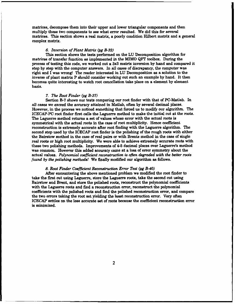
matrices, decompose them into their upper and lower triangular components and thenmultiply these two components to see what error resulted. We did this for severalmatrices. This section shows a real matrix, a poorly condition Hilbert matrix and a generalcomplex matrix.
6. Inversion of Plant Matrix (pg B-32)This section shows the tests performed on the LU Decomposition algorithm for
matrices of transfer function as implemented in the MIMO QFT toolbox. During theprocess of testing this code, we worked out a 3x3 matrix inversion by hand and compared itstep by step with the computer answers. In all cases of discrepancy, the computer wasright and I was wrong! The reader interested in LU Decomposition as a solution to theinverse of plant matrix P should consider working out such an example by hand. It thenbecomes quite interesting to watch root cancellation take place on a element by elementbasis.
7. The Root Finder (pg B-37)Section B-7 shows our tests comparing our root finder with that of PC-Matlab. In
all cases we exceed the accuracy attained in Matlab, often by several decimal places.However, in the process we noticed something that forced us to modify our algorithm. TheICECAP-PC root finder first calls the Laguerre method to make the initial cut at the roots.The Laguerre method returns a set of values whose error with the actual roots issymmetrical with the actual roots in the case of root multiplicity. Hence coefficientreconstruction is extremely accurate after root finding with the Laguerre algorithm. Thesecond step used by the ICECAP root finder is the polishing of the rough roots with eitherthe Bairstow method in the case of real pairs or with Brents method in the case of singlereal roots or high root multiplicity. We were able to achieve extremely accurate roots withthese two polishing methods. Improvements of 4-5 decimal places over Laguerre's methodwas common. However this added accuracy came at a loss of error symmetry about theactual values. Polynomial coefficient reconstruction is often degraded with the better rootsfound by the polishing methods! We finally modified our algorithm as follows.
8. Root Finder Coefficient Reconstruction Error Test (pg B-40)After encountering the above mentioned problem we modified the root finder to
take the first cut using Laguerre, store the Laguerre roots, take the second cut usingBairstow and Brent, and store the polished roots, reconstruct the polynomial coefficientswith the Laguerre roots and find a reconstruction error, reconstruct the polynomialcoefficients with the polished roots and find the polished reconstruction error, and comparethe two errors taking the root set yielding the least reconstruction error. Very oftenICECAP settles on the less accurate set of roots because the coefficient reconstruction erroris minimized.
2
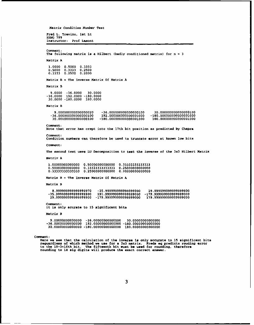
Matrix Condition Number Test
Fred L. Trevino, 1st LtEENG 799Instructor: Prof Lamont
Comment:
The following matrix is a Hilbert (badly conditioned matrix) for n 3
Matrix A
1.0000 0.5000 0.33330.5000 0.3333 0.25000.3333 0.2500 0.2000
Matrix B = The Inverse Matrix Of Matrix A
Matrix B
9.0000 -36.0000 30.0000-36.0000 192.0000 -180.000030.0000 -180.0000 180.0000
Matrix B
9.000000000000000020 -36.000000000000000100 30.000000000000000100-36.000000000000000100 192.000000000000001000 -180.000000000000001000
30.000000000000000100 -180.000000000000001000 180.000000000000001000
Comment:Note that error has crept into the 17th bit position as predicted by Chapra
Comment:Condition numbers can therefore be used to truncate error at known low bits
Comment:
The second test uses LU Decomposition to test the inverse of the 3x3 Hilbert Matrix
Matrix A
1.00000000000000 0.50000000000000 0.333333333333330.50000000000000 0.33333333333333 0.250000000000000.33333333333333 0.25000000000000 0.20000000000000
Matrix B = The Inverse Matrix Of Matrix A
Matrix B
8.999999999999999970 -35.999999999999999900 29.999999999999999900-35.999999999999999900 191.999999999999999000 -179.99999999999999900029.999999999999999900 -179.999999999999999000 179.999999999999999000
Comment:it is only acurate to 15 significant bits
Matrix B
9.00000000000000 -36.00000000000000 30.00000000000000-36.00000000000000 192.00000000000000 -180.00000000000000
30.00000000000000 -180.00000000000000 180.00000000000000
Comment:Here we see that the calculation of the inverse is only accurate to 15 significant bitsreguardless of which method we use for a 3x3 matrix. Freds eq predicts rouding errorto the 19-3=16th bit. The fifteenth bit must be used for rounding, thereforerounding to 14 sig digits will produce the exact correct answer.
3

Eigenvalues using QR Shift
Fred L. Trevino25 June 92Thim is a test of Dr Jones QR Shift Algorithm for a general complex matrixwith single eigenvalues. This will validate the formation of the Householdermatrix by the method taught by Dr Jones.
a=
1.0000 + 1.0000i 4.0000 - 2.0000i 3.0000 - 1.0000i4.0000 + 2.0000i 4.0000 6.0000 + 8.0000i
0 + 1.0000i 3.0000 1.0000 + 7.0000i
SInMat = balance(a)
InMat =
1.0000 + 1.0000i 4.0000 - 2.0000i 1.5000 - 0.5000i4.0000 + 2.0000i 4.0000 3.0000 + 4.0000i
0 + 2.0000i 6.0000 1.0000 + 7.0000i
InMat = hess(InMat)
InMat =
1.0000 + 1.0000i 4.1079 - 1.3693i 1.3693 + 1.3693i4.3818 + 2.1909i 3.6667 + 0.8333i 4.9333 + 6.3000i
0 3.0000 + 0.1667i 1.3333 + 6.1667i
SeigtstW Undefined function or variable.
Symbol in question -^P eigtst
Seigentst
-----.Main Menu
1) Input Matrix2) Specify Ctr3) Run Test4) Display Result5) Quit
Select a menu number:Enter Iteration Count:
Ctr =
25
Ctr =
25
Press Enter To Continue
-----.Main Menu
1) Input Matrix2) Specify Ctr3) Run Test4) Display Result5) Quit
Select a menu number: Running .....Iteration:
i=
4
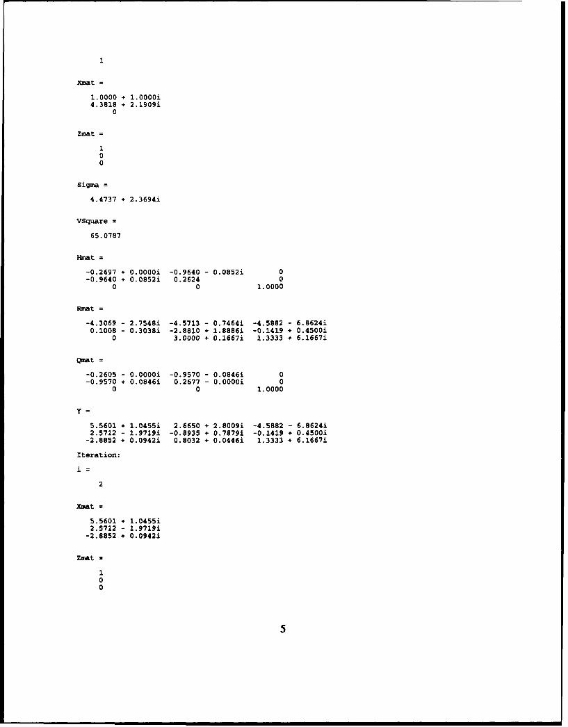
Xmat =
1.0000 + 1.0000i4.3818 + 2.1909i
0
Zmat =
100
Sigma =
4.4737 + 2.3694i
VSquare =
65.0787
Hmat =
-0.2697 + 0.0000i -0.9640 - 0.0852i 0-0.9640 + 0.0852i 0.2624 0
0 0 1.0000
Rmat =
-4.3069 - 2.7548i -4.5713 - 0.7464i -4.5882 - 6.8624i0.1008 - 0.3038i -2.8810 + 1.8886i -0.1419 + 0.4500i
0 3.0000 + 0.1667i 1.3333 + 6.1667i
Omat =
-0.2605 - 0.0000i -0.9570 - 0.0846i 0-0.9570 + 0.0846i 0.2677 - 0.0000i 0
0 0 1.0000
y =
5.5601 + 1.0455i 2.6650 + 2.8009± -4.5882 - 6.8624i2.5712 - 1.9719i -0.8935 + 0.7879i -0.1419 + 0.4500i
-2.8852 + 0.0942i 0.8032 + 0.0446± 1.3333 + 6.1667i
Iteration:
i=
2
Xmat =
5.5601 + 1.0455i2.5712 - 1.97191
-2.8852 + 0.09421
Zmat=
100
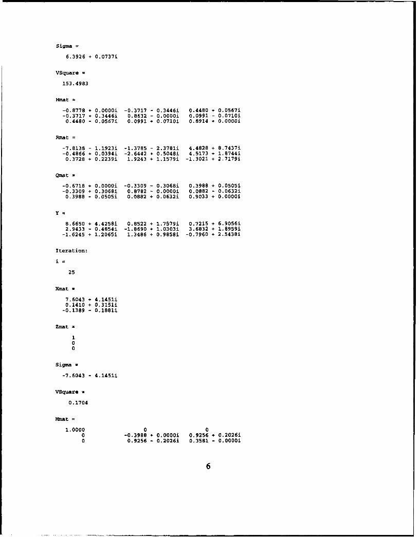
Sigma =
6.3926 + 0.0737i
VSquare =
153.4983
Hmat =
-0.8778 + 0.0000i -0.3717 - 0.3446i 0.4480 + 0.0567i-0.3717 + 0.3446i 0.8632 - 0.0000i 0.0991 - 0.0710i0.4480 - 0.0567i 0.0991 + 0.0710i 0.8914 + 0.0000i
Rmat =
-7.8138 - 1.1923i -1.3785 - 2.3781i 4.4828 + 8.7437i-0.4866 + 0.0394i -2.6442 + 0.5048i 4.5173 + 1.8744i0.3728 + 0.2239i 1.9243 + 1.1579i -1.3021 + 2.7179i
Qmat =
-0.6718 + 0.0000i -0.3309 - 0.3068i 0.3988 + 0.0505i-0.3309 + 0.3068i 0.8782 - 0.0000i 0.0882 - 0.0632i0.3988 - 0.0505i 0.0882 + 0.0632i 0.9033 + 0.0000i
y =
8.6650 + 4.4258i 0.8522 + 1.7579± 0.7215 + 6.9056i2.9433 - 0.4854i -1.8690 + 1.0303i 3.6832 + 1.8959i
-1.6245 + 1.2065i 1.3486 + 0.9858i -0.7960 + 2.5438i
Iteration:
i=
25
Xmat =
7.6043 + 4.1451i0.1410 + 0.3151i
-0.1389 - 0.1881i
Zmat=
100
Sigma =
-7.6043 - 4.1451±
VSquare =
0.1704
Hmat =
1.0000 0 00 -0.3988 + 0.00001 0.9256 * 0.2026i0 0.9256 - 0.20261 0.3581 - 0.0000i
6
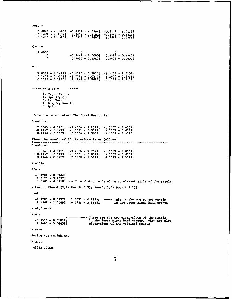
Rmat =
7.6043 + 4.1451i -2.6219 - 6.2994i -0.4115 - 5.0033i-0.1467 - 0.3279i 3.5471 - 1.2151i -0.4863 - 0.6414i0.1446 + 0.1957i 0.0817 + 2.9607i 1.7685 + 3.2964i
Qmat =
1.0000 0 00 -0.3441 - 0.0000i 0.8895 + 0.1947i0 0.8895 - 0.1947i 0.3832 + 0.0000i
Y =
7.6043 + 4.1451i -0.4380 - 2.2024± -1.2532 - 8.0309i-0.1467 - 0.3279i -1.7781 - 0.0577i 3.2053 - 0.6359i
0.1446 + 0.1957i 2.1868 + 1.5689i 0.1739 + 3.9125i
----- Main Menu
1) Input Matrix2) Specify Ctr3) Run Test4) Display Result5) Quit
Select a menu number: The Final Result Is:
Result =
7.6043 + 4.1451i -0.4380 - 2.2024i -1.2632 - 8.0309i-0.1467 - 0.3279i -1.7781 - 0.0577± 3.2053 - 0.6359i
0.1446 + 0.1957i 2.1868 + 1.5689i 0.1739 + 3.9125i
%Now, the result of 25 iterations is as follows:
Result =
7.6043 + 4.1451i -0.4380 - 2.2024i -1.2632 - 8.0309i-0.1467 - 0.3279i -1.7781 - 0.0577i 3.2053 - 0.6359i
0.1446 + 0.1957i 2.1868 + 1.5689i 0.1739 + 3.9125i
eig(a)
ans =
-3.4786 + 0.5744i1.8179 + 3.4037i7.6607 + 4.0219i <- Note that this is close to element (1,1) of the result
Stest = [Result(2,2) Result(2,3); Result(3,2) Result(3,3)]
test =
-1.7781 - 0.0577i 3.2053 - 0.6359i r-> This is the two by two matrix2.1868 + 1.5689i 0.1739 + 3.9125i± in the lower right hand corner
eig(test)
ans => These are the two eigenvalues of the matrix
-3.4530 + 0.5103i in the lower right hand corner. They are also1.8487 + 3.3445i± eigenvalues of the original matrix.
save
Saving to: matlab.mat
Squit
42652 flops.
7

The QR Shift Algorithm Imnplemented in ICECAP
Fred L. TrevinoEENG 799Prof Gary I Lamont
: QRShift Test
Matrix C
0.0000 1.0000 0.00000.0000 0.0000 1.00006.0000 -1.0000 -4.0000
Balanced Form of Matrix C
0.0000 2.0000 0.00000.0000 0.0000 1.00003.0000 -1.0000 -4.0000
Hess-berg Form of Balanced Matrix C
0.0000 0.0000 2.00003.0000 -4.0000 -1.00000.0000 1.00n0 0.0000
TP 1TP 2TP 3TP 3TP 4TP 6TP 10TP 12
its 1nn: 3
P: 0.2500q: 0.0000r: 0.7500S: 1.3333t: 0.0000U: 0.55637508958790268E+0105v: 0.0000x: 0.00Vy: -4.0000z: 0.0000Eigenvalue 1 0.0000 0.0000Eigenvalue 2 0.0000 0.0000Eigenvalue 3 0.0000 0.0000TP 18TP 19TP 20TP 22TP 23
its 1nn: 3
p: 0.0000q: 0.0000r: 0.72088: 0.7906t: 0.0000U: 0.55637508958790268E+0105v: 0.0000x: 1.3162y: 0.0000Z: 0.9487Eigenvalue 1 0.0000 0.0000Eigenvalue 2 0.0000 0.0000Eigenvalue 3 0.0000 0.0000
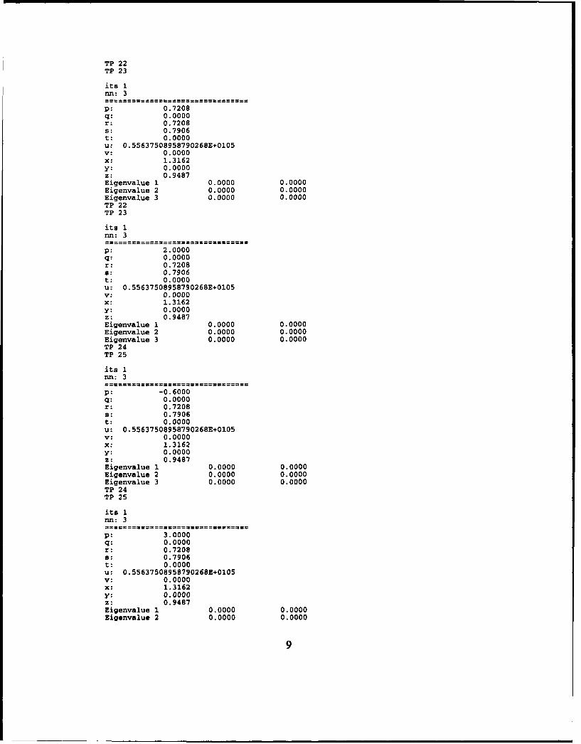
TP 22TP 23
its 1nf: 3
P: 0.7208Q: 0.0000r: 0.7208S: 0.7906t: 0.0000U: 0.55637508958790268E+0105v: 0.0000x: 1.3162y: 0.0000z: 0.9487Eigenvalue 1 0.0000 0.0000Eigenvalue 2 0.0000 0.0000Eigenvalue 3 0.0000 0.0000TP 22TP 23
its 1nn: 3
p: 2.0000q: 0.0000r: 0.7208s: 0.7906t: 0.0000u: 0.55637508958790268E+0105v: 0.0000x: 1.3162y: 0.0000Z: 0.9487Eigenvalue 1 0.0000 0.0000Eigenvalue 2 0.0000 0.0000Eigenvalue 3 0.0000 0.0000TP 24TP 25
its 1nn: 3
P: -0.6000Q: 0.0000r: 0.72088: 0.7906t: 0.0000u: 0.55637508958790268E+0105v: 0.0000x: 1.3162y: 0.0000z: 0.9487Eigenvalue 1 0.0000 0.0000Eigenvalue 2 0.0000 0.0000Eigenvalue 3 0.0000 0.0000TP 24TP 25
its 1Fin: 3
p: 3.00000.0000
r: 0.7208s: 0.7906t: 0.0000U: 0.55637508958790268E+0105v: 0.0000X: 1.3162y: 0.0000Z: 0.9487Eigenvalue 1 0.0000 0.0000Eigenvalue 2 0.0000 0.0000
9
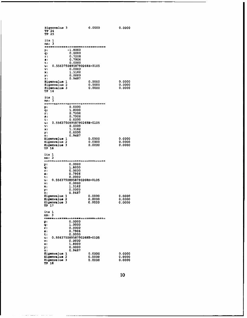
Eigenvalue 3 0.0000 0.0000TP 24TP 25
its 1nn: 3
p: -1.8000Q: 0.0000r: 0.7208s: 0.7906t: 0.0000u: 0.55637508958790268E+0105v: 0.0000x: 1.3162y: 0.0000z: 0.9487Eigenvalue 1 0.0000 0.0000Eigenvalue 2 0.0000 0.0000Eigenvalue 3 0.0000 0.0000TP 14
its 1nn: 3
p: 0.0000q: 1.8000r: 0.7208s: 0.7906t: 0.0000u: 0.55637508958790268E+0105v: 0.0000x: 1.3162y: 0.0000z: 0.9487Eigenvalue 1 0.0000 0.0000Eigenvalue 2 0.0000 0.0000Eigenvalue 3 0.0000 0.0000TP 16
its 1nn: 3
P: 0.0000q: 1.8000r: 0.00008: 0.7906t: 0.0000u: 0.55637508958790268E+0105v: 0.0000x: 1.3162y: 0.0000z: 0.9487Eigenvalue 1 0.0000 0.0000Eigenvalue 2 0.0000 0.0000Eigenvalue 3 0.0000 0.0000TP 17
its 1nn: 3
p: 0.0000Q: 1.0000r: 0.00008: 0.7906t: 0.0000u: 0.55637508958790268E+0105v: 0.0000x: 1.8000y: 0.0000z : 0.9487Eigenvalue 1 0.0000 0.0000Eigenvalue 2 0.0000 0.0000Eigenvalue 3 0.0000 0.0000TP 18
10

TP 19TP 21TP 22TP 22TP 24TP 24TP 24TP 26TP 3TP 3TP 4TP 6TP 10TP 12
its 2nn: 3
P: -0.3060q: 0.4113r: -0.2827s: 11.1845t: 0.0000U: 0.55637508958790268E+0105v: 0.0000x: -4.0000y: -0.6000Z: 0.6000Eigenvalue 1 0.0000 0.0000Eigenvalue 2 0.0000 0.0000Eigenvalue 3 0.0000 0.0000TP 18TP 19TP 20TP 22TP 23
its 2nn: 3
P: 1.4305q: -0.4614r: 0.31728: -0.5854t: 0.0000U: 0.55637508958790268E+0105v: 0.0000x: 1.5227y: -0.7025z: 0.4830Eigenvalue 1 0.0000 0.0000Eigenvalue 2 0.0000 0.0000Eigenvalue 3 0.0000 0.0000TP 22TP 23
its 2nn: 3
P: -0.5262q: -0.4614r: 0.31728: -0.5854t: 0.0000u: 0.55637508958790268E+0105v: 0.0000x: 1.5227y: -0.7025z: 0.4830Eigenvalue 1 0.0000 0.0000Eigenvalue 2 0.0000 0.0000Eigenvalue 3 0.0000 0.0000TP 22TP 23
11
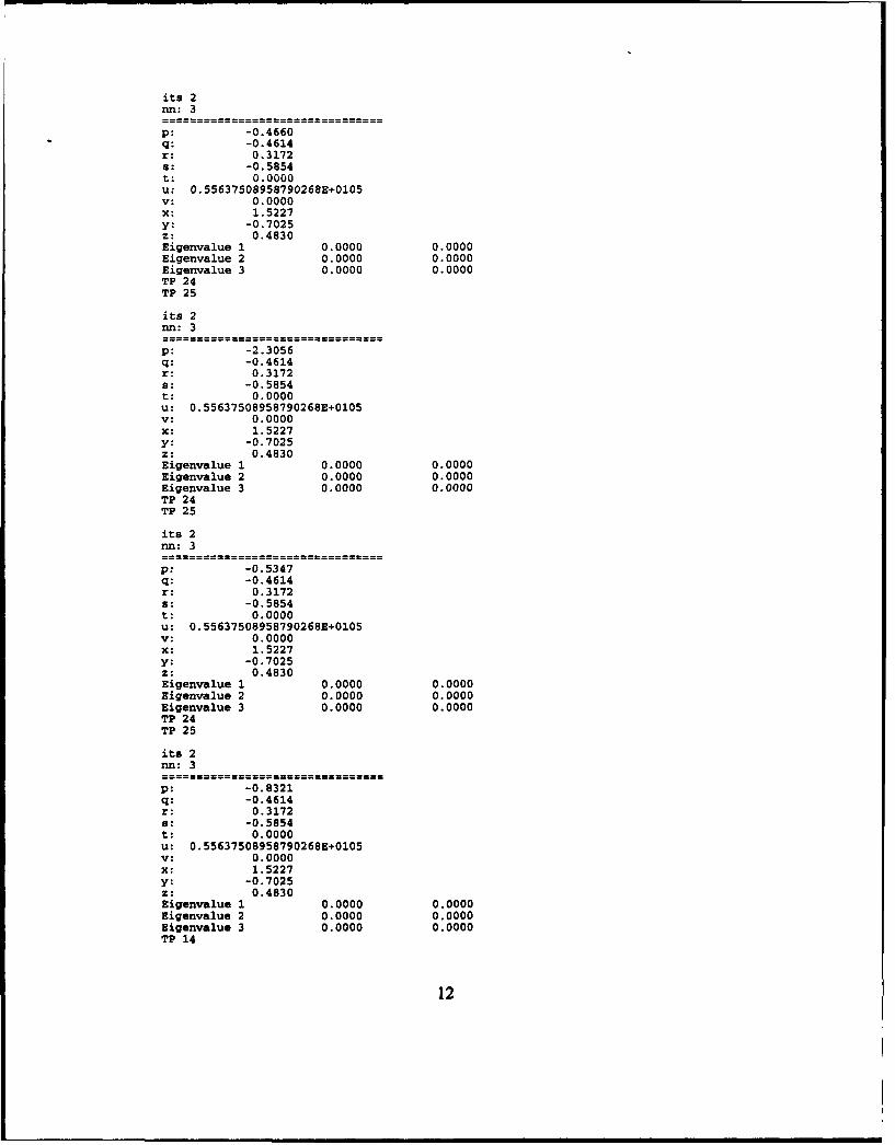
its 2nn: 3
p: -0.4660q: -0.4614r: 0.3172s: -0.5854t: 0.0000u: 0.55637508958790268E+0105v: 0.0000x: 1.5227y: -0.7025z: 0.4830Eigenvalue 1 0.0000 0.0000Eigenvalue 2 0.0000 0.0000Eigenvalue 3 0.0000 0.0000TP 24TP 25
its 2nn: 3
p: -2.3056q: -0.4614r: 0.3172s: -0.5854t: 0.0000U: 0.55637508958790268E+0105v: 0.0000x: 1.5227y: -0.7025z: 0.4830Eigenvalue 1 0.0000 0.0000Eigenvalue 2 0.0000 0.0000Eigenvalue 3 0.0000 0.0000TP 24TP 25
its 2nn: 3
-0.5347q: -0.4614r: 0.31728: -0.5854t: 0.0000u: 0.55637508958790268E+0105v: 0.0000X: 1.5227y: -0.7025z: 0.4830Eigenvalue 1 0.0000 0.0000Eigenvalue 2 0.0000 0.0000Eigenvalue 3 0.0000 0.0000TP 24TP 25
its 2nn: 3
p: -0.8321q: -0.4614r: 0.3172a: -0.5854t: 0.0000u: 0.55637508958790268E+0105v: 0.0000x: 1.5227y: -0.7025Z: 0.4830Eigenvalue 1 0.0000 0.0000Eigenvalue 2 0.0000 0.0000Eigenvalue 3 0.0000 0.0000TP 14
12
its 2nn: 3
p: -0.2603q: 0.1412r: 0.3172a: -0.5854t: 0.0000u: 0.55637508958790268E+0105v: 0.0000x: 1.5227y: -0.7025z: 0.4830Eigenvalue 1 0.0000 0.0000Eigenvalue 2 0.0000 0.0000Eigenvalue 3 0.0000 0.0000TP 16
its 2nn: 3
P: -0.2603Q: 0.1412r: 0.0000s: -0.5854t: 0.0000u: 0.55637508958790268E+0105v: 0.0000x: 1.5227y: -0.7025z: 0.4830Eigenvalue 1 0.0000 0.0000Eigenvalue 2 0.0000 0.0000Eigenvalue 3 0.0000 0.0000TP 17
its 2nn: 3
p: -0.6484q: 0.3516r: 0.0000s: -0.5854t: 0.0000u: 0.55637508958790268E+0105v: 0.0000x: 0.4015y: -0.7025z: 0.4830Eigenvalue 1 0.0000 0.0000Eigenvalue 2 0.0000 0.0000Eigenvalue 3 0.0000 0.0000TP 18TP 19TP 21TP 22TP 22TP 24TP 24TP 24TP 26TP 3TP 3TP 4TP 6TP 10TP 12
its 3nn: 3
0.8223q: 0.1344r: 0.0432a: 37.4230
13
t : 0.0000u: 0.55637508958790268E+0105v: 0.0000x: -4.3027y: -0.4247z: 0.7274Eigenvalue 1 0.0000 0.0000Eigenvalue 2 0.0000 0.0000Eigenvalue 3 0.0000 0.0000TP 18TP 19TP 20TP 22TP 23
its 3nn: 3
P: 0.7514q: 0.0811r: 0.0261s: 0.8344t: 0.0000u: 0.55637508958790268E+0105v: 0.0000x: 1.9856y: 0.1611z: 0.0518Eigenvalue 1 0.0000 0.0000Eigenvalue 2 0.0000 0.0000Eigenvalue 3 0.0000 0.0000TP 22TP 23
its 3nn: 3
P: 1.2018q: 0.0811r: 0.0261s: 0.8344t: 0.0000u: 0.55637508958790268E+0105v: 0.0000x: 1.9856y: 0.1611z: 0.0518Eigenvalue 1 0.0000 0.0000Eigenvalue 2 0.0000 0.0000Eigenvalue 3 0.0000 0.0000TP 22TP 23
its 3nn: 3
P: 1.8097q: 0.0811r: 0.02618: 0.8344t: 0.0000u: 0.55637508958790268E+0105v: 0.0000x: 1.9856y: 0.1611z: 0.0518Eigenvalue 1 0.0000 0.0000Eigenvalue 2 0.0000 0.0000Eigenvalue 3 0.0000 0.0000TP 24TP 25
its 3nn: 3
14
P: -1.7892Q: 0.0811r: 0.0261s: 0.8344t: 0.0000u: 0.55637508958790268E+0105v: 0.0000x: 1.9856y: 0.1611z: 0.0518Eigenvalue 1 0.0000 0.0000Eigenvalue 2 0.0000 0.0000Eigenvalue 3 0.0000 0.0000TP 24TP 25
its 3nn: 3
p: 0.1380q: 0.0811r: 0.0261s: 0.8344t: 0.0000u: 0.55637508958790268E+0105v: 0.0000x: 1.9856y: 0.1611z: 0.0518Eigenvalue 1 0.0000 0.0000Eigenvalue 2 0.0000 0.0000Eigenvalue 3 0.0000 0.0000TP 24TP 25
its 3nn: 3
p: -0.0545q: 0.0811r: 0.0261s: 0.8344t: 0.0000u: 0.55637508958790268E+0105v: 0.00Gjx: 1.9856y: 0.1611z: 0.0518Eigenvalue 1 0.0000 0.0000Eigenvalue 2 0.0000 0.0000Eigenvalue 3 0.0000 0.0000TP 14
its 3nn: 3
P: 0.0371q: 0.0156r: 0.0261s: 0.8344t: 0.0000U: 0.55637508958790268E+0105v: 0.0000x: 1.9856y: 0.1611z: 0.0518Eigenvalue 1 0.0000 0.0000Eigenvalue 2 0.0000 0.0000Eigenvalue 3 0.0000 0.0000TP 16
its 3n: 3
P: 0.0371
15

0.0156r: 0.0000a: 0.8344t: 0.0000u: 0.55637508958790268E+0105v: 0.0000X: 1.9856y: 0.1611z: 0.0518Eigenvalue 1 0.0000 0.0000Eigenvalue 2 0.0000 0.0000Eigenvalue 3 0.0000 0.0000TP 17
its 3nn: 3
P: 0.7042q: 0.2958r: 0.00008: 0.8344t: 0.0000U: 0.55637508958790268E+0105V: 0.0000X: 0.0527y: 0.1611z: 0.0518Eigenvalue 1 0.0000 0.0000Eigenvalue 2 0.0000 0.0000Eigenvalue 3 0.0000 0.0000TP 18TP 19TP 21TP 22TP 22TP 24TP 24TP 24TP 26TP 3TP 3TP 4TP 6TP 10TP 12
its 4nn: 3
p: -0.9840q: 0.0151r: -0.00108: 308.7020t: 0.0000U: 0.55637508958790268E+0105v: 0.0000X: -3.6282y: -1.3963z: 1.0246Eigenvalue 1 0.0000 0.0000Eigenvalue 2 0.0000 0.0000Eigenvalue 3 0.0000 0.0000TP 18TP 19TP 20TP 22TP 23
its 4nn: 3
P: 1.0249q: -0.0077r: 0.00058: -0.9841
16
t: 0.0000u: 0.55637508958790268E+0105v* 0.0000x. 1.9999y: -0.0153z: 0.0010Eigenvalue 1 0.0000 0.0000Eigenvalue 2 0.0000 0.0000Eigenvalue 3 0.0000 0.0000TP 22TP 23
its 4nf: 3
p: 1.5475q: -0.0077r: 0.0005s: -0.9841t: 0.0000U: 0.55637508958790268E+0105v: 0.0000x: 1.9999y: -0.0153z: 0.0010Eigenvalue 1 0.0000 0.0000Eigenvalue 2 0.0000 0.0000Eigenvalue 3 0.0000 0.0000TP 22TP 23
its 4nn: 3
P: -0.9831Q: -0.0077r: 0.0005s: -0.9841t: 0.0000U: 0.55637508958790268E+0105v: 0.0000x: 1.9999y: -0.0153Z: 0.0010Eigenvalue 1 0.0000 0.0000Eigenvalue 2 0.0000 0.0000Eigenvalue 3 0.0000 0.0000TP 24TP 25
its 4nn: 3
p: -2.0252q: -0.0077r: 0.00058: -0.9841t: 0.0000u: 0.55637508958790268E+0105v: 0.0000x: 1.9999y: -0.0153z: 0.0010Eigenvalue 1 0.0000 0.0000Eigenvalue 2 0.0000 0.0000Eigenvalue 3 0.0000 0.0000TP 24TP 25
its 4nn: 3
-0.0247-0.0077
r: 0.0005
17
S: -0.9841t: 0.0000u: 0.55637508958790268E+0105v: 0.0000x: 1.9999y: -0.0153z: 0.0010Eigenvalue 1 0.0000 0.0000Eigenvalue 2 0.0000 0.0000Eigenvalue 3 0.0000 0.0000TP 24TP 25
its 4nn: 3
P: -0.0010q: -0.0077r: 0.0005s: -0.9841t: 0.0000u: 0.55637508958790268E+0105v: 0.0000x,. 1.9999y: -0.0153z: 0.0010Eigenvalue 1 0.0000 0.0000Eigenvalue 2 0.0000 0.0000Eigenvalue 3 0.0000 0.0000TP 14
its 4nn: 3
p: 0.0002q: -0.0000r: 0.0005s: -0.9841t: 0.0000u: 0.55637508958790268E+0105v: 0.0000x: 1.9999y: -0.0153z: 0.0010Eigenvalue 1 0.0000 0.0000Eigenvalue 2 0.0000 0.0000Eigenvalue 3 0.0000 0.0000TP 16
its 4nn: 3
P: 0.0002q: -0.0000r: 0.0000s: -0.9841t: 0.0000u: 0.55637508958790268E+0105v: 0.0000x: 1.9999y: -0.0153z: 0.0010Eigenvalue 1 0.0000 0.0000Eigenvalue 2 0.0000 0.0000Eigenvalue 3 0.0000 0.0000TP 17
its 4nn: 3
P: 0.8760q: -0.1240r: 0.0000a: -0.9841t: 0.0000
18
U: 0.55637508958790268E+0105v: 0.0000x: 0.0002y: -0.0153z: 0.0010Eigenvalue 1 0.0000 0.0000Eigenvalue 2 0.0000 0.0000Eigenvalue 3 0.0000 0.0000TP 18TP 19TP 21TP 22TP 22TP 24TP 24TP 24TP 26TP 3TP 3TP 4TP 6TP 10TP 12
its 5nn: 3
P: -0.9999q: 0.0001r: 0.0000s: 69288.8960t: 0.0000u: 0.55637508958790268E+0105V: 0.0000X: -3.1570y: -1.8431z: 1.0001Eigenvalue 1 0.0000 0.0000Eigenvalue 2 0.0000 0.0000Eigenvalue 3 0.0000 0.0000TP 18TP 19TP 20TP 22TP 23
its 5nn: 3
p: 1.0001Q: -0.0000r: -0.0000s: -0.9999t: 0.0000U: 0.55637508958790268E+0105v: 0.0000x: 2.0000y: -0.0001z: -0.0000Eigenvalue 1 0.0000 0.0000Eigenvalue 2 0.0000 0.0000Eigenvalue 3 0.0000 0.0000TP 22TP 23
its 5nn: 3
P: 1.6997q: -0.0000r: -0.00008: -0.9999t: 0.0000u: 0.55637508958790268E+0105v: 0.0000
19
x: 2.0000y: -0.0001z : -0.0000Eigenvalue 1 0.0000 0.0000Eigenvalue 2 0.0000 0.0000Eigenvalue 3 0.0000 0.0000TP 22TP 23
its 5nn: 3
P: 0.7813-0.0000
r: -0.0000S: -0.9999t: 0.0000u: 0.55637508958790268E+0105v: 0.0000x: 2.0000y: -0.0001z: -0.0000Eigenvalue 1 0.0000 0.0000Eigenvalue 2 0.0000 0.0000Eigenvalue 3 0.0000 0.0000TP 24TP 25
its 5nn: 3
P: -2.0001q: -0.0000r: -0.0000s: -0.9999t: 0.0000u: 0.55637508958790268E+0105v: 0.0000x: 2.0000y: -0.0001z: -0.0000Eigenvalue 1 0.0000 0.0000Eigenvalue 2 0.0000 0.0000Eigenvalue 3 0.0000 0.0000TP 24TP 25
its 5nn: 3
p: -0.0001q: -0.0000r: -0.0000S: -0.9999t: 0.0000U: 0.55637508958790268E+0105v: 0.0000x: 2.0000y: -0.0001z: -0.0000Eigenvalue 1 0.0000 0.0000Eigenvalue 2 0.0000 0.0000Eigenvalue 3 0.0000 0.0000TP 24TP 25
its 5nn: 3
p: 0.0000q. -0.0000r: -0.00005: -0.9999t, 0.0000U: 0.55637508958790268E+0105
20
V: 0.0000x: 2.0000y: -0.0001z : -0.0000Eigenvalue 1 0.0000 0.0000Eigenvalue 2 0.0000 0.0000Eigenvalue 3 0.0000 0.0000TP 14
its 5nn: 3
P: 0.0000q: 0.0000r, -0.0000s: -0.9999t: 0.0000u: 0.55637508958790268E+0105V: 0.0000x: 2.0000y: -0.0001Z: -0.0000Eigenvalue 1 0.0000 0.0000Eigenvalue 2 0.0000 0.0000Eigenvalue 3 0.0000 0.0000TP 16
its 5nn: 3
P: 0.0000q: 0.0000r: 0.0000S: -0.9999t: 0.0000u: 0.55637508958790268E+0105V:. 0.0000x: 2.0000Y: -0.0001z: -0.0000Eigenvalue 1 0.0000 0.0000Eigenvalue 2 0.0000 0.0000Eigenvalue 3 0.0000 0.0000TP 17
its 5nn: 3
P: 0.9625q: 0.0375r: 0.0000a: -0.9999t: 0.0000u: 0.55637508958790268E+0105V: 0.0000X: 0.0000y: -0.0001z: -0.0000Eigenvalue 1 0.0000 0.0000Eigenvalue 2 0.0000 0.0000Eigenvalue 3 0.0000 0.0000TP 18TP 19TP 21TP 22TP 22TP 24TP 24TP 24TP 26TP 3TP 3TP 4TP 6TP 10
21
TP 12
its 6nn: 3
P: -1.0000q: 0.0000r: -0.0000s: 6298606684.8862t: 0.0000U: 0.55637508958790268E+0105v: 0.0000x: -3.0160y: -1.9840z: 1.0000Eigenvalue 1 0.0000 0.0000Eigenvalue 2 0.0000 0.0000Eigenvalue 3 0.0000 0.0000TP 18TP 19TP 20TP 22TP 23
its 6nn: 3
p: 1.0000q: -0.0000r: 0.0000s: -1.0000t: 0.0000U: 0.556375089587S0268E+0105v: 0.0000x: 22.0000y: -0.0000z: 00.0000Eigenvalue 1 0.0000 0.0000Eigenvalue 2 0.0000 0.0000Eigenvalue 3 0.0000 0.0000TP 22TP 23
its 6nn: 3
p: 1.7290q: -0.0000r: 00.0000s: -1.0000t: 0.0000u: 0.55637508958790268E+0105v: 0.0000x: 2.0000y : -0.0000z: 0.0000Eigenvalue 1 0.0000 0.0000Eigenvalue 2 0.0000 0.0000Eigenvalue 3 0.0000 0.0000TP 22TP 23
its 6nn: 3
p: -0.7146q: -0.0000r: 00.00008 : -1.0000t: 0.0000U: 0.55637508958790268E+0105v: 0.0000x: 2.0000y : -0.0000z: 0.0000
22
Eigenvalue 1 0.0000 0.0000Eigenvalue 2 0.0000 0.0000Eigenvalue 3 0.0000 0.0000TP 24TP 25
its 6nn: 3
P . .- 2.0000q: -0.0000r: 0.00008: -1.0000t: 0.0000U: 0.55637508958790268E÷0105v: 0.0000X: 2.0000y: -0.0000z : 0.0000Eigenvalue 1 0.0000 0.0000Eigenvalue 2 0.0000 0.0000Eigenvalue 3 0.0000 0.0000TP 24TP 25
its 6nn: 3
p: -0.0000q: -0.0000r: 0.0000a: -1.0000t: 0.0000U: 0.55637508958790268E+0105v: 0.0000x: 2.0000y: -0.0000z: 0.0000Eigenvalue 1 0.0000 0.0000Eigenvalue 2 0.0000 0.0000Eigenvalue 3 0.0000 0.0000TP 24TP 25
its 6nn: 3
P: =-0.0000q: -0.0000r: -0.00008: -1.0000t: 0.0000u: 0.55637508958790268E+0105v: 0.0000x: 2.0000y: -0.0000z: 0.0000Eigenvalue 1 0.0000 0.0000Eigenvalue 2 0.0000 0.0000Eigenvalue 3 0.0000 0.0000TP 14
its 6nn: 3
p: 0.0000q: -0.0000r: 0.00008: -1.0000t: 0.0000U: 0.55637508958790268E+0105V: 0.0000x: 2.0000y: -0.0000z: 0.0000
23
Eigenvalue 1 0.0000 0.0000Eigenvalue 2 0.0000 0.0000Eigenvalue 3 0.0000 0.0000TP 16
its 6nn: 3
p: 0.0000q: -0.0000r: 0.0000s: -1.0000t: 0.0000U: 0.55637508958790268E+0105V: 0.0000x: 2.0000y: -0.0000z: 0.0000Eigenvalue 1 0.0000 0.0000Eigenvalue 2 0.0000 0.0000Eigenvalue 3 0.0000 0.0000TP 17
its 6nn: 3
P: 0.9957q: -0.0043r: 0.0000s: -1.0000t: 0.0000U: 0.55637508958790268E+0105v: 0.0000x: 0.0000y: -0.0000z: 0.0000Eigenvalue 1 0.0000 0.0000Eigenvalue 2 0.0000 0.0000Eigenvalue 3 0.0000 0.0000TP 18TP 19TP 21TP 22TP 22TP 24TP 24TP 24TP 26TI 3TP 3TP 4TP 6TP 10TP 12
its 7nn: 3
P: -1.0000q: 0.0000r: 0.0000a: 66626453394759628100.0000t: 0.0000U: 0.55637508958790268E+0105v: 0.0000x: -3.0002y: -1.9998z: 1.0000Eigenvalue 1 0.0000 0.0000Eigenvalue 2 0.0000 0.0000Eigenvalue 3 0.0000 0.0000TP 18TP 19TP 20TP 22
24
TP 23
its 7nn: 3
P: 1.0000q: -0.0000r: -0.0000s: -1.0000t: 0.0000u: 0.55637508958790268E+0105v: 0.0000x: 2.0000y: -0.0000z: -0.0000Eigenvalue 1 0.0000 0.0000Eigenvalue 2 0.0000 0.0000Eigenvalue 3 0.0000 0.0000TP 22TP 23
its 7nn: 3
p: 1.7320q: -0.0000r: -0.0000s: -1.0000t: 0.0000u: 0.55637508958790268E+0105v: 0.0000x: 2.0000y: -0.0000z: -0.0000Eigenvalue 1 0.0000 0.0000Eigenvalue 2 0.0000 0.0000Eigenvalue 3 0.0000 0.0000TP 22TP 23
its 7nn: 3
p: 0.7072q: -0.0000r: -0.0000s: -1.0000t: 0.0000U: 0.55637508958790268E+0105v: 0.0000x: 2.0000y: -0.0000z : -0.0000Eigenvalue 1 0.0000 0.0000Eigenvalue 2 0.0000 0.0000Eigenvalue 3 0.0000 0.0000TP 24TP 25
its 7nn: 3
P: -2.0000q: -0.0000r: -0.00002: -1.0000t: 0.0000u: 0.55637508958790268E+0105v: 0.0000x: 2.0000y: -0.0000z: -0.0000Eigenvalue 1 0.0000 0.0000Eigenvalue 2 0.0000 0.0000Eigenvalue 3 0.0000 0.0000
25
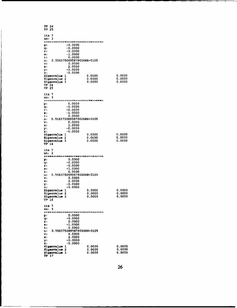
TP 24TP 25
its 7in: 3
-0.0000-0.0000
r: -0.0000s: -1.0000t: 0.0000u: 0.55637508958790268E+0105v: 0.0000x: 2.0000y: -0.0000z: -0.0000Eigenvalue 1 0.0000 0.0000Eigenvalue 2 0.0000 0.0000Eigenvalue 3 0.0000 0.0000TP 24TP 25
its 7nn: 3
p: 0.0000q: -0.0000r: -0.0000s: -1.0000t: 0.0000u: 0.55637508958790268E+0105v: 0.0000x: 2.0000y: -0.0000z: -0.0000Eigenvalue 1 0.0000 0.0000Eigenvalue 2 0.0000 0.0000Eigenvalue 3 0.0000 0.0000TP 14
its 7nn: 3
P: 0.0000q: -0.0000r: -0.0000s: -1.0000t: 0.0000U: 0.55637508958790268E+0105v: 0.0000x: 2.0000y: -0.0000z: -0.0000Eigenvalue 1 0.0000 0.0000Eigenvalue 2 0.0000 0.0000Eigenvalue 3 0.0000 0.0000TP 16
its 7nn: 3
P: 0.0000q: -0.0000r: 0.00008: -1.0000t: 0.0000U: 0.55637508958790268E+0105V: 0.0000X: 2.0000y: -0.0000z: -0.0000Eigenvalue 1 0.0000 0.0000Eigenvalue 2 0.0000 0.0000Eigenvalue 3 0.0000 0.0000TP 17
26
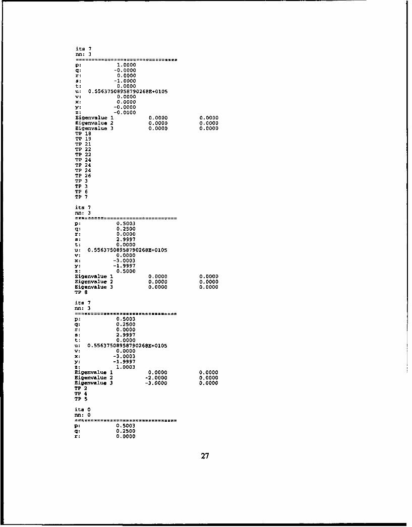
its 7nn: 3
P: 1.0000q: -0.0000r: 0.0000s: -1.0000t: 0.0000U: 0.55637508958790268E+0105v: 0.0000x: 0.0000y: -0.0000z: -0.0000Eigenvalue 1 0.0000 0.0000Eigenvalue 2 0.0000 0.0000Eigenvalue 3 0.0000 0.0000TP 18TP 19TP 21TP 22TP 22TP 24TP 24TP 24TP 26TP 3TP 3TP 6TP 7
its 7nn: 3
p: 0.5003q: 0.2500r: 0.0000S: 2.9997t: 0.0000u: 0.55637508958790268E+0105v: 0.0000x: -3.0003y: -1.9997z: 0.5000Eigenvalue 1 0.0000 0.0000Eigenvalue 2 0.0000 0.0000Eigenvalue 3 0.0000 0.0000TP 8
its 7nn: 3
P: 0.5003q: 0.2500r: 0.0000s: 2.9997t: 0.0000u: 0.55637508958790268E+0105v: 0.0000x: -3.0003y: -1.9997z: 1.0003Eigenvalue 1 0.0000 0.0000Eigenvalue 2 -2.0000 0.0000Eigenvalue 3 -3.0000 0.0000TP 2TP 4TP 5
its 0nn: 0
P: 0.5003q: 0.2500r: 0.0000
27
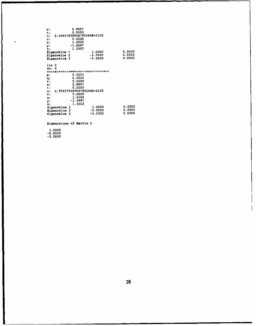
s: 2.9997t: 0.0000U: 0.55637508958790268E+0105v: 0.0000x: 1.0000y: -1.9997z: 1.0003Eigenvalue 1 1.0000 0.0000Eigenvalue 2 -2.0000 0.0000Eigenvalue 3 -3.0000 0.0000
its 0nn: 0
P: 0.5003q: 0.2500r: 0.0000s: 2.9997t: 0.0000u: 0.55637508958790268E+0105v: 0.0000x: 1.0000y: -1.9997z: 1.0003Eigenvalue 1 1.0000 0.0000Eigenvalue 2 -2.0000 0.0000Eigenvalue 3 -3.0000 0.0000
Eigenvalues of Matrix C
1.0000-2.0000-3.0000
28
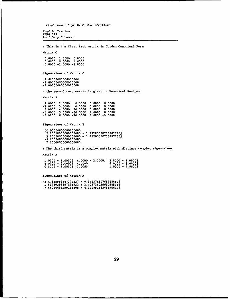
Final Test of QR Shift For ICECAP-PC
Fred L. TrevinoEENG 799Prof Gary I Lamont
: This is the first test matrix in Jordan Canonical Form
Matrix C
0.0000 1.0000 0.00000.0000 0.0000 1.00006.0000 -1.0000 -4.0000
Eigenvalues of Matrix C
1.00000000000000000-3.00000000000000000-2.00000000000000000
: The second test matrix is given in Numerical Recipes
Matrix E
1.0000 2.0000 0.0000 0.0000 0.0000-2.0000 3.0000 0.0000 0.0000 0.0000
3.0000 4.0000 50.0000 0.0000 0.0000-4.0000 5.0000 -60.0000 7.0000 0.0000-5.0000 6.0000 -70.0000 8.0000 -9.0000
Eigenvalues of Matrix E
50.000000000000000002.00000000000000000 - 1.73205080756887730j2.00000000000000000 + 1.73205080756887730j
-9.000000000000000007.00000000000000000
The third matrix is a complex matrix with distinct complex eigenvalues
Matrix A
1.0000 + 1.0000j 4.0000 - 2.0000j 3.0000 - 1.0000j4.0000 + 2.0000j 4.0000 6.0000 + 8.0000j0.0000 + 1.0000j 3.0000 1.0000 + 7.0000j
Eigenvalues of Matrix A
-3.47855955887271427 + 0.57437430768745852j1.81789299597115922 + 3.40373402863058531j7.66066656290155505 + 4.02189166368195617j
29

LU Decompsition
Fred L. TrevinoEENG 799Prof Gary I Lamont
Comment:This is a test of the LU Decomposition Method. I will Decompose three matricies,
multiply them back together and compare.
Matrix A
0.000000000000000 1.000000000000000 0.0000000000000000.000000000000000 0.000000000000000 1.0000000000000006.000000000000000 -1.000000000000000 -4.000000000000000
The LU Decomposition is Given By:
L Component
1.000000000000000 0.000000000000000 0.0000000000000000.000000000000000 1.000000000000000 0.0000000000000000.000000000000000 0.000000000000000 1.000000000000000
U Component
6.000000000000000 -1.000000000000000 -4.0000000000000000.000000000000000 1.0000OU0000000000 0.0000000000000000.000000000000000 0.000000000000000 1.000000000000000
The L and U Components Multiplied Together Equal:
Matrix B
0.000000000000000 1.000000000000000 0.0000000000000000.000000000000000 0.000000000000000 1.0000000000000006.000000000000000 -1.000000000000000 -4.000000000000000
Matrix A
0.000000000000000 1.000000000000000 0.0000000000000000.000000000000000 0.000000000000000 1.0000000000000006.000000000000000 -l.0000JO000000000 -4.000000000000000
Comment:This was a Jordan Canonical Form Matrix
Comment:
Comment:
The second test is to to a 5x5 Hilbert matrix
Matrix I
1.000000000000000 0.500000000000000 0.333333333333333 0.2500000000000000.200000000000000
0.500000000000000 0.333333333333333 0.250000000000000 0.2000000000000000.166666666666667
0.333333333333333 0.250000000000000 0.200000000000000 0.1666666666666670.142857142857143
0.250000000000000 0.200000000000000 0.166666666666667 0.1428571428571430.125000000000000
0.200000000000000 0.166666666666667 0.142857142857143 0.1250000000000000.111111111111111
The LU Decomposition is Given By:
L Component
1.000000000000000 0.000000000000000 0.000000000000000 0.0000000000000000.000000000000000
30
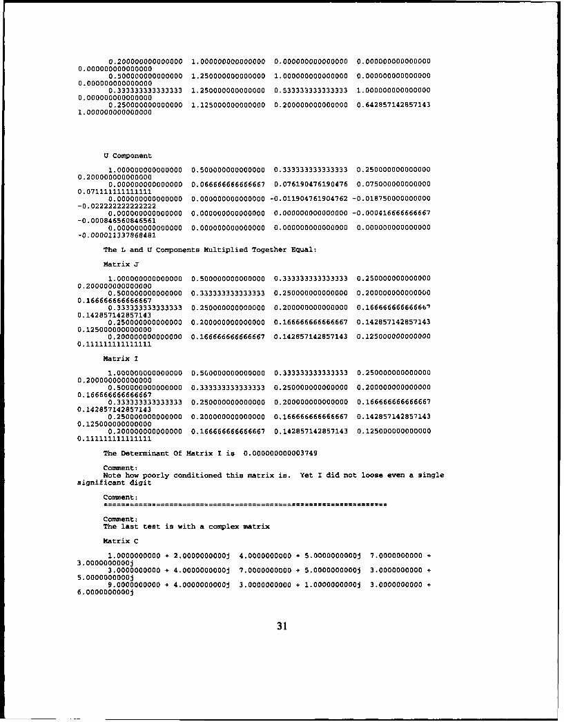
0.200000000000000 1.000000000000000 0.000000000000000 0.0000000000000000.000000000000000
0.500000000000000 1.250000000000000 1.000000000000000 0.0000000000000000.000000000000000
0.333333333333333 1.250000000000000 0.533333333333333 1.0000000000000000.000000000000000
0.250000000000000 1.125000000000000 0.200000000000000 0.6428571428571431.000000000000000
U Component
1.000000000000000 0.500000000000000 0.333333333333333 0.2500000000000000.200000000000000
0.000000000000000 0.066666666666667 0.076190476190476 0.0750000000000000.071111111111111
0.000000000000000 0.000000000000000 -0.011904761904762 -0.018750000000000-0.022222222222222
0.000000000000000 0.000000000000000 0.000000000000000 -0.000416666666667-0.000846560846561
0.000000000000000 0.000000000000000 0.000000000000000 0.000000000000000-0.000011337868481
The L and U Components Multiplied Together Equal:
Matrix J
1.000000000000000 0.500000000000000 0.333333333333333 0.2500000000000000.200000000000000
0.500000000000000 0.333333333333333 0.250000000000000 0.2000000000000000.166666666666667
0.333333333333333 0.250000000000000 0.200000000000000 0.1666666666666b60.142857142857143
0.250000000000000 0.200000000000000 0.166666666666667 0.1428571428571430.125000000000000
0.200000000000000 0.166666666666667 0.142857142857143 0.1250000000000000.111111111111111
Matrix I
1.000000000000000 0.500000000000000 0.333333333333333 0.2500000000000000.200000000000000
0.500000000000000 0.333333333333333 0.250000000000000 0.2000000000000000.1666666666666667
0.333333333333333 0.250000000000000 0.200000000000000 0.1666666666666670.142857142857143
0.250000000000000 0.200000000000000 0.166666666666667 0.1428571428571430.125000000000000
0.200000000000000 0.166666666666667 0.142857142857143 0.1250000000000000.111111111111111
The Determinant Of Matrix I is 0.000000000003749
Comment:Note how poorly conditioned this matrix is. Yet I did not loose even a single
significant digit
Comment:
Comment:
The last test is with a complex matrix
Matrix C
1.0000000000 + 2.OOOOOOOOOOj 4.0000000000 + 5.0000000000j 7.0000000000 +3.0000000000j
3.0000000000 + 4.0000000000j 7.0000000000 + 5.0000000000j 3.0000000000 +5.0000000000j
9.0000000000 + 4.OOOOOOOOOOj 3.0000000000 + 1.0000000000j 3.0000000000 +6.OOOOOOOOOOj
31
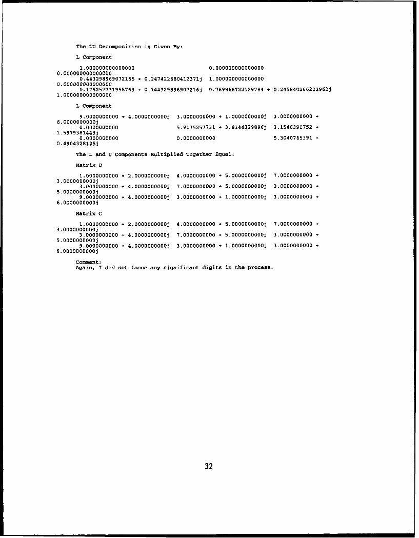
The LU Decomposition is Given By:
L Component
1.000000000000000 0.0000000000000000.000000000000000
0.443298969072165 + 0.247422680412371j 1.0000000000000000.000000000000000
0.175257731958763 + 0.144329896907216j 0.769966722129784 + 0.245840266222962j1.000000000000000
L Component
9.0000000000 + 4.0000000000j 3.0000000000 + 1.0000000000j 3.0000000000 +6.0000000000j
0.0000000000 5.9175257731 + 3.8144329896j 3.1546391752 +1.5979381443j
0.0000000000 0.0000000000 5.3040765391 -0.4904328125j
The L and U Components Multiplied Together Equal:
Matrix D
1.0000000000 + 2.0000000000j 4.0000000000 + 5.0000000000j 7.0000000000 +3.0000000000j
3.0000000000 + 4.0000000000j 7.0000000000 + 5.0000000000j 3.0000000000 +5.0000000000j
9.0000000000 + 4.0000000000j 3.0000000000 + 1.0000000000j 3.0000000000 +6.0000000000j
Matrix C
1.0000000000 + 2.0000000000j 4.0000000000 + 5.0000000000j 7.0000000000 +3.0000000000j
3.0000000000 + 4.0000000000j 7.0000000000 + 5.0000000000j 3.0000000000 +5.0000000000j
9.0000000000 + 4.0000000000j 3.0000000000 + 1.0000000000j 3.0000000000 +6.0000000000j
Comment:Again, I did not loose any significant digits in the process.
32
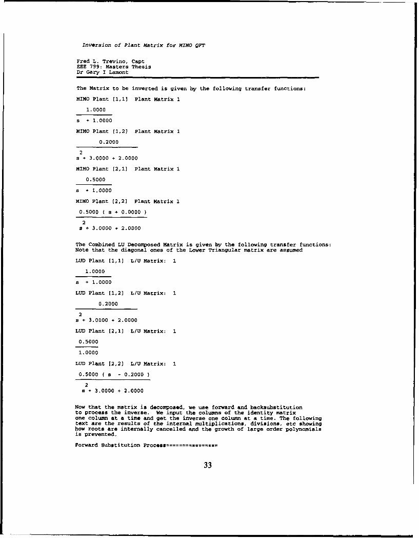
Inversion of Plant Matrix for MIMO QFT
Fred L. Trevino, CaptEEE 799: Masters ThesisDr Gary I Lamont
The Matrix to be inverted is given by the following transfer functions:
MIMO Plant [1,1] Plant Matrix 1
1.0000
s + 1.0000
MIMO Plant [1,2] Plant Matrix 1
0.2000
2s + 3.0000 + 2.0000
MIMO Plant [2,1] Plant Matrix 1
0.5000
s + 1.0000
MIMO Plant [2,2] Plant Matrix 1
0.5000 ( s + 0.0000
2a + 3.0000 + 2.0000
The Combined LU Decomposed Matrix is given by the following transfer functions:Note that the diagonal ones of the Lower Triangular matrix are assumed
LUD Plant [1,1] L/U Matrix: 1
1.0000
s + 1.0000
LUD Plant [1,2] L/U Matrix: 1
0.2000
2s + 3.0000 + 2.0000
LUD Plant [2,1] L/U Matrix: 1
0.5000
1.0000
LUD Plant [2,2] L/U Matrix: 1
0.5000 ( s - 0.2000
2s + 3.0000 + 2.0000
Now that the matrix is decomposed, we use forward and backsubstitutionto process the inverse. We input the columns of the identity matrixone column at a time and get the inverse one column at a time. The followingtext are the results of the internal multiplications, divisions, etc showinghow roots are internally cancelled and the growth of large order polynomialsis prevented.
Forward Substitution Process================
33
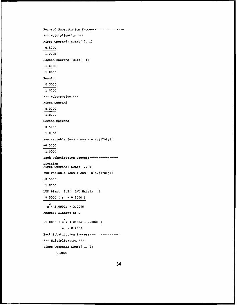
Forward Substitution Process================
*** Multiplication ***
First Operand: LUmat( 2, 1]
0.5000
1.0000
Second Operand: BMat 1 1]
1.0000
1.0000
Result
0.5000
1.0000
*** Subtraction ***
First Operand
0.0000
1.0000
Second Operand
0.5C00
1.0000
sum variable (sum = sum - a[i,j]*b[j])
-0.5000
1.0000
Back Substitution Process================
DivisionFirst Operand: LUmat[ 2, 2]
sum variable (sum = sum - a[i,j]*b[j])
-0.5000
1.0000
LUD Plant [2,2] L/U Matrix: 1
0.5000 ( a 0.2000
2s e 3.00009 + 2.0000
Answer: Element of Q
2-1.0000 ( a + 3.0000s + 2.0000
s - 0.2000
Back Substitution Process==
*** Multiplication ***
First Operand: LUmat[ 1, 2]
0.2000
34

28 , 3.0000s + 2.0000
Second Operand: EMat C 2]
2-1.0000 ( s + 3.0000s + 2.0000
a - 0.2000
Result
-0.2000
s - 0.2000
**Subtraction**
First Operand
1. 0000
1 .0000
Second Operand
-0. 2000
S- 0.2000
sum variable (sum =sum -a~i,jl~b[l))
a + 0.0000
s - 0.2000
Division
First Operand: LUmat] 1, 1]
a + 0.0000
s - 0.2000
Second Operand:
1.0000
s + 1.0000
Answer: Element of0
2s + 1.00008+ 0.0000
a-0.2000IForward Substitution Process=--------------
Forward Substitution Process========
Back Substitution Process================-
DivisionFirst Operand: LUmatt 2, 2]
One
1.0000
1.0000
35
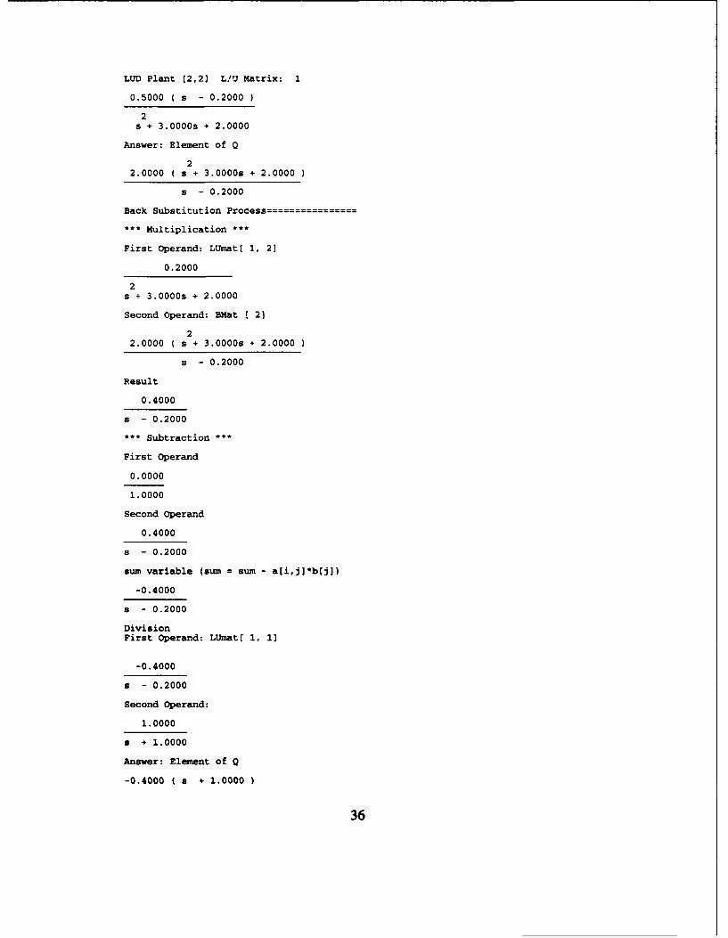
LUD Plant [2,2] L/U Matrix: 1
0.5000 ( s - 0.2000
2
S + 3.0000s + 2.0000
Answer: Element of Q
22.0000 ( s + 3.0000s + 2.0000
s - 0.2000
Back Substitution Process===
*** Multiplication ***
First Operand: LUmat( 1, 2]
0.2000
2s + 3.0000s + 2.0000
Second Operand: BMat 1 2]
2
2.0000 ( s + 3.0000s + 2.0000
s - 0.2000
Result
0.4000
s - 0.2000
*** Subtraction *
First Operand
0.0000
1.0000
Second Operand
0.4000
s - 0.2000
sum variable (sum = sum - a[i,j]*b(j])
-0.4000
s - 0.2000
DivisionFirst Operand: LUmat[ 1, 1]
-0.4000
s - 0.2000
Second Operand:
1.0000
s + 1.0000
Answer: Element of Q
-0.4000 C s + 1.0000
36
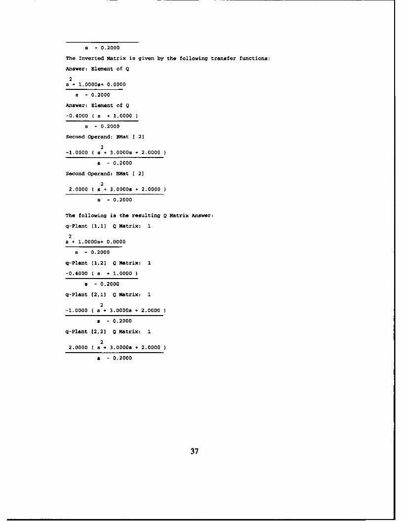
a - 0.2000
The Inverted Matrix is given by the following transfer functions:
Answer: Element of Q
2s + 1.0000s+ 0.0000
s - 0.2000
Answer: Element of Q
-0.4000 ( a + 1.0000
s - 0.2000
Second Operand: BMat [ 2]
2-1.0000 ( s + 3.0000s + 2.0000
s - 0.2000
Second Operand: BMat [ 2]
22.0000 ( s + 3.0000s + 2.0000
s - 0.2000
The following is the resulting Q Matrix Answer:
q-Plant [1,1] Q Matrix: 1
2s + 1.0000s+ 0.0000
a - 0.2000
q-Plant [1,2] Q Matrix: 1
-0.4000 ( a + 1.0000
s - 0.2000
q-Plant [2,1] Q Matrix: 1
2-1.0000 ( s + 3.0000s + 2.0000
a - 0.2000
q-Plant [2,2] Q Matrix: 1
22.0000 ( s + 3.0000s + 2.0000
s - 0.2000
37
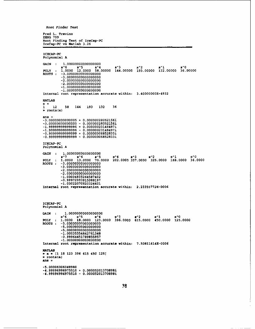
Root Finder Test
Fred L. TrevinoEENG 799Root Finding Test of IceCap-PCIceCap-PC vs Matlab 3.26
ICECAP-PCPolynomial A
GAIN 1.00000000000000000s^6 s^5 s^4 s^3 s^2 s'l s^0
POLY : 1.0000 12.0000 58.00000 144.00000 193.00000 132.00000 36.00000ROOTS -3.00000000000000000
-3.00000000000000000-2.00000000000000000-2.00000000000000000-1.00000000000000000-1.00000000000000000
Internal root representation accurate within: 3.40000000E-4932
MATLABe =1 12 58 144 193 132 36o roots(e)
ans =-3.00000000000005 + 0.00000028052156i-3.00000000000005 - 0.00000028052156i-1.99999999999996 + 0.00000023148497i-1.99999999999996 - 0.00000023148497i-0.99999999999999 + 0.00000006852833i-0.99999999999999 - 0.00000006852833i
ICECAP-PCPolynomial A
GAIN : 1.00000000000000000s^7 s^6 s^5 s^4 s^3 s^2 s^1 s^0
POLY : 1.0000 13.0000 70.0000 202.0000 337.0000 325.0000 168.0000 36.0000ROOTS -3.00000000000000000
-3.00000000000000000-2.00000000000000000-2.00000000000000000-1.00004935264587402-0.99972993915088197-1.00022070820324401
Internal root representation accurate within: 2.23355772E-0006
ICECAP-PCPolynomial A
GAIN : 1.00000000000000000s^6 s^5 s^4 s^3 s^2 s^1 s^0
POLY : 1.0000 18.0000 123.0000 396.0000 615.0000 450.0000 125.0000ROOTS : -5.00000000000000000
-5. 00000000000000000-5.00000000000000000-1.00035554842761348-0.99964451789855957-1.00000000000000000
Internal root representation accurate within: 7.50811614E-0006
MATLABa = E1 18 123 396 615 450 1251
Sroots(a)ans =
-5.00006006048980-4.99996996975510 + 0.00005201370898i-4.99996996975510 - 0.00005201370898i
38
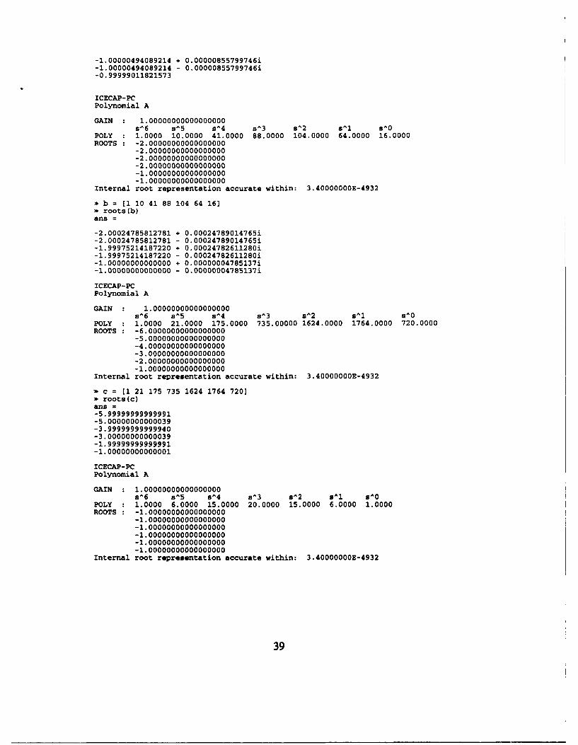
-1.00000494089214 + 0.00000855799746i-1.00000494089214 - 0.00000855799746i-0.99999011821573
ICECAP-PCPolynomial A
GAIN 1.00000000000000000s^6 s^5 s^4 s^3 s^2 s^l s^0
POLY 1.0000 10.0000 41.0000 88.0000 104.0000 64.0000 16.0000ROOTS : -2.00000000000000000
-2.00000000000000000-2.00000000000000000-2.00000000000000000-1.00000000000000000-1.00000000000000000
Internal root representation accurate within: 3.40000000E-4932
* b = [1 10 41 88 104 64 16]* roots(b)ans =
-2.00024785812781 + 0.00024789014765i-2.00024785812781 - 0.00024789014765i-1.99975214187220 + 0.00024782611280i-1.99975214187220 - 0.00024782611280i-1.00000000000000 + 0.00000004785137i-1.00000000000000 - 0.00000004785137i
ICECAP-PCPolynomial A
GAIN : 1.00000000000000000s^6 s^5 s^4 s^3 s^2 s^l s^0
POLY 1.0000 21.0000 175.0000 735.00000 1624.0000 1764.0000 720.0000ROOTS : -6.00000000000000000
-5.00000000000000000-4.00000000000000000-3.00000000000000000-2.00000000000000000-1.00000000000000000
Internal root representation accurate within: 3.40000000E-4932
Sc = (1 21 175 735 1624 1764 720]roots(c)
ans =-5.99999999999991-5.00000000000039-3.99999999999940-3.00000000000039-1.99999999999991-1.00000000000001
ICECAP-PCPolynomial A
GAIN : 1.00000000000000000s^6 s^5 s^4 s^3 s^2 s^l s^0
POLY : 1.0000 6.0000 15.0000 20.0000 15.0000 6.0000 1.0000ROOTS : -1.00000000000000000
-1.00000000000000000-1.00000000000000000-1.00000000000000000-1.00000000000000000-1.00000000000000000
Internal root representation accurate within: 3.40000000E-4932
39
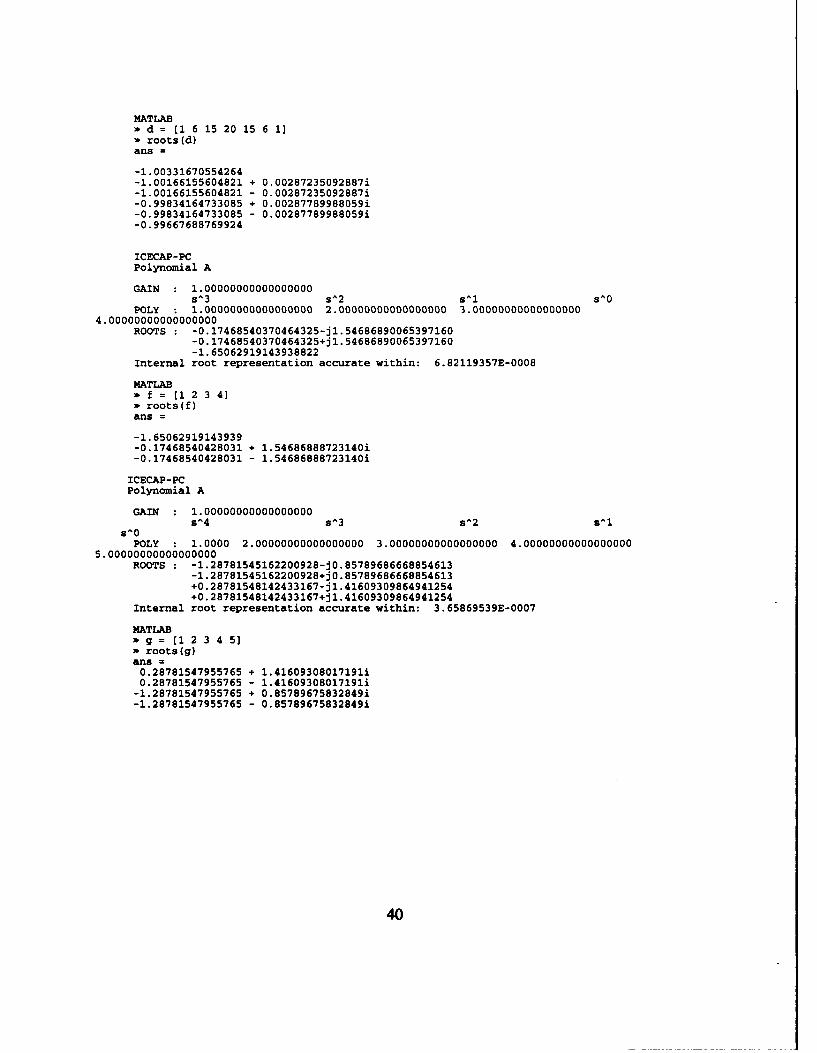
MATLABSd = [1 6 15 20 15 6 1]* roots (d)ans =
-1.00331670554264-1.00166155604821 + 0.00287235092887i-1.00166155604821 - 0.00287235092887i-0.99834164733085 + 0.00287789988059i-0.99834164733085 - 0.00287789988059i-0.99667688769924
ICECAP-PCPolynomial A
GAIN 1.00000000000000000s^3 s^2 s^l s^0
POLY : 1.00000000000000000 2.00000000000000000 3.000000000000000004.00000000000000000
ROOTS : -0.17468540370464325-jl.54686890065397160-0.17468540370464325+jl.54686890065397160-1.65062919143938822
Internal root representation accurate within: 6.82119357E-0008
MATLAB*f = [1 2 3 4]Sroots(f)ans =
-1.65062919143939-0.17468540428031 + 1.54686888723140i-0.17468540428031 - 1.54686888723140i
ICECAP-PCPolynomial A
GAIN : 1.00000000000000000s^4 s^3 s^2 s^l
s^0POLY : 1.0000 2.00000000000000000 3.00000000000000000 4.00000000000000000
5.00000000000000000ROOTS : -1.28781545162200928-jO.85789686668854613
-1.28781545162200928+j0.85789686668854613+0.28781548142433167-jl.41609309864941254+0.28781548142433167+jl.41609309864941254
Internal root representation accurate within: 3.65869539E-0007
MATLABg = (1 2 3 4 5]roots(g)
ans =0.28781547955765 + 1.41609308017191i0.28781547955765 - 1.41609308017191i
-1.28781547955765 + 0.85789675832849i-1.28781547955765 - 0.85789675832849i
40

Root Finder Coefficient Reconstruction Error TestFred L. Trevino, Capt, USAFElectrical Engineer
Unpolished Polynomial
Polynomial AGAIN : 1.0000
s^6 s^5 s^4 s^3 s^2 s^l s^0POLY : 1.0000 12.0000 58.0000 144.0000 193.0000 132.0000 36.0000ROOTS -0.99999986114853990
-1.00000013885151794-1.99999958484187777-2.00000041515827876-2.99999971614412451-3.00000028385566112
Internal root representation accurate within: 2.40238385E-0013 %
Unpolished Accuracy: 2.40238384741076E-0013
Polished Polynomial
Polynomial AGAIN : 1.0000
s^6 s^5 s^4 s^3 s^2 s^l s^0POLY : 1.0000 12.0000 58.0000 144.0000 193.0000 132.0000 36.0000ROOTS : -1.00000000000000000
-1.00000000000000000-2.00000000000000000-2.00000000000000000-3.00000000000000000-3.00000000000000000
Internal root representation accurate within: 0.OOOOOOOOE+0000 %
Polished Accuracy: 0.OOOOOOOOOOOOOOE+0000
Choosing Polished Polynomial
Unpolished Polynomial
Polynomial AGAIN : 1.0000
s^7 s^6 s^5 s^4 s^3 s^2 s^l s^0POLY : 1.0000 13.0000 70.0000 202.0000 337.0000 325.0000 168.0000 36.0000ROOTS : -0.99995061525371413
-1.00002469237289833-1.00002469786131161-1.99991445853344107-2.00008554146667941-2.99995722634657145-3.00004276816538401
Internal root representation accurate within: 7.31758333E-0009 %
Unpolished Accuracy: 7.31758333094579E-0009
Polished Polynomial
Polynomial AGAIN : 1.0000
s^7 s^6 s^5 s^4 s^3 s^2 s^1 s^0POLY : 1.0000 13.0000 70.0000 202.0000 337.0000 325.0000 168.0000 36.0000ROOTS : -1.00000114885965188
-1.00000082939761701-0.99999965957871331-2.00000000000000000-2.00000000000000000-3.00000000000000000-3.00000000000000000
Internal root representation accurate within: 5.89621054E-0005 %
41
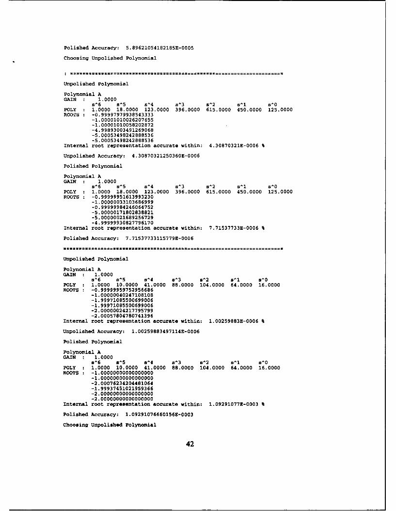
Polished Accuracy: 5.89621054182185E-0005
Choosing Unpolished Polynomial
Unpolished Polynomial
Polynomial AGAIN : 1.0000
s^6 s^5 s^4 s^3 s^2 s^l s^0POLY 1.0000 18.0000 123.0000 396.0000 615.0000 450.0000 125.0000ROOTS : -0.99997979938543333
-1.00001010026207655-1.00001010058202872-4.99893003491269068-5.00053498242888536-5.00053498242888536
Internal root representation accurate within: 4.30870321E-0006 %
Unpolished Accuracy: 4.30870321250360E-0006
Polished Polynomial
Polynomial AGAIN : 1.0000
s^6 s^5 s^4 s^3 s^2 s^l s^0POLY : 1.0000 18.0000 123.0000 396.0000 615.0000 450.0000 125.0000ROOTS : -0.99999951613993230
-1.00000033103686999-0.99999984246064752-5.00000171802838821-5.00000021689256729-4.99999930827796170
Internal root representation accurate within: 7.71537733E-0006 %
Polished Accuracy: 7.71537733115779E-0006
Unpolished Polynomial
Polynomial AGAIN : 1.0000
s^6 s^5 s^4 s^3 s^2 s^l s^0POLY : 1.0000 10.0000 41.0000 88.0000 104.0000 64.0000 16.0000ROOTS : -0.99999959752956686
-1.00000040247108108-1.99971085500699006-1.99971085500699006-2.00000024217795799-2.00057804780741396
Internal root representation accurate within: 1.00259883E-0006 %
Unpolished Accuracy: 1.00259883497114E-0006
Polished Polynomial
Polynomial AGAIN : 1.0000
s^6 s^5 s^4 s^3 s^2 s^1 s^0POLY : 1.0000 10.0000 41.0000 88.0000 104.0000 64.0000 16.0000ROOTS : -1.00000000000000000
-1.00000000000000000-2.00076234204481064-1.99937451021959366-2.00000000000000000-2.00000000000000000
Internal root representation accurate within: 1.09291077E-0003 %
Polished Accuracy: 1.09291076660156E-0003
Choosing Unpolished Polynomial
42

Unpolished Polynomial
Polynomial AGAIN 1.0000
s^6 s^5 s^4 s^3 s^2 s^l s^0POLY : 1.0000 21.0000 175.0000 735.0000 1624.0000 1764.0000 720.0000ROOTS -0.99999999999999868
-2.00000000000000659-2.99999999999998685-4.00000000000001295-4.99999999999999379-6.00000000000000114
Internal root representation accurate within: 1.59872116E-0013 %
Unpolished Accuracy: 1.59872115546023E-0013
Polished Polynomial
Polynomial AGAIN : 1.0000
s^6 s^5 s^4 s^3 s^2 s^l s^0POLY : 1.0000 21.0000 175.0000 735.0000 1624.0000 1764.0000 720.0000ROOTS : -2.00000000000000000
-1.00000000000000000-4.00000000000000000-3.00000000000000000-6.00000000000000000-5.00000000000000000
Internal root representation accurate within: 0.OOOOOOOOE+0000 %
Polished Accuracy: 0.OOOOOOOOOOOOOOE+0000
Unpolished Polynomial
Polynomial AGAIN : 1.0000
s^6 s^5 s^4 s^3 s^2 8^1 sA0POLY : 1.0000 6.0000 15.0000 20.0000 15.0000 6.0000 1.0000ROOTS : -1.00000000000000000
-1.00000000000000000-1.00000000000000000-1.00000000000000000-1.00000000000000000-1.00000000000000000
Internal root representation accurate within: 0.OOOOOOOOE+0000 %
Unpolished Accuracy: 0.00000000000000E+0000
Polished Polynomial
Polynomial AGAIN : 1.0000
s^6 s^5 s^4 s^3 s-2 sAl s^0POLY : 1.0000 6.0000 15.0000 20.0000 15.0000 6.0000 1.0000ROOTS : -1.00000000000000000
-1.00000000000000000-1.00000000000000000-1.00000000000000000-1.00000000000000000-1.00000000000000000
Internal root representation accurate within: 0.OOOOOOOOE+0000 %
Polished Accuracy: 0.00000000000000E+0000
Choosing Polished Polynomial
Unpolished Polynomial
43

Polynomial AGAIN 1.0000
s^3 s^2 s^l s^OPOLY : 1.0000 2.0000 3.0000 4.0000ROOTS : -0.17468540428030588-jl.54686888723139627
-0.17468540428030589+jl.54686888723139628-1.65062919143938823
Internal root representation accurate within: 2.36419161E-0017 %
Unpolished Accuracy: 2.36419160587147E-0017
Polished Polynomial
Polynomial AGAIN : 1.0000
s^3 s^2 s8l s^0POLY : 1.0000 2.0000 3.0000 4.0000ROOTS : -0.17468540428030588-jl.54686888723139624
-0.17468540428030588+jl.54686888723139624-1.65062919143938822
Internal root representation accurate within: 2.19008839E-0016 %
Polished Accuracy: 2.19008838842072E-0016
Choosing Unpolished Polynomial
Unpolished Polynomial
Polynomial AGAIN : 1.0000
s^4 s^3 s^2 s^l s^O
POLY : 1.0000 2.0000 3.0000 4.0000 5.0000ROOTS : -1.28781547955764792+jO.85789675832849048
-1.28781547955764819-j0.85789675832849027+0.28781547955764808+jl.41609308017190785+0.28781547955764803-jl.41609308017190806
Internal root representation accurate within: 1.61971028E-0015 %
Unpolished Accuracy: 1.61971028480621E-0015
Polished Polynomial
Polynomial AGAIN : 1.0000s^4 s^3 s^2 s^l s^0
POLY : 1.0000 2.0000 3.0000 4.0000 5.0000ROOTS : -1.28781547955764797-jO.85789675832849028
-1.28781547955764797+jO.85789675832849028+0.28781547955764797-jl.41609308017190794+0.28781547955764797+jl.41609308017190794
Internal root representation accurate within: 1.58293526E-0016 %
Polished Accuracy: 1.58293526465436E-0016
Choosing Unpolished Polynomial
44
Appendix C ICECAP-PC User's Manual
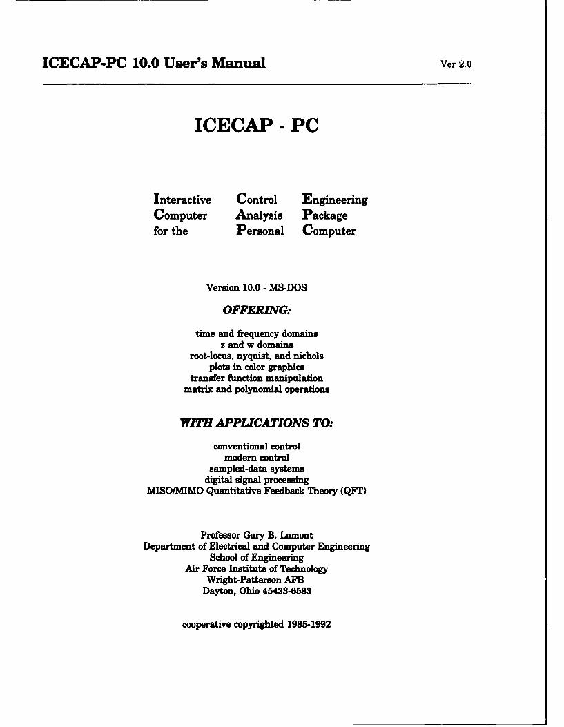
ICECAP-PC 10.0 User's Manual Ver 2.0
ICECAP- PC
Interactive Control EngineeringComputer Analysis Packagefor the Personal Computer
Version 10.0 - MS-DOS
OFFERING:
time and frequency domainsz and w domains
root-locus, nyquist, and nicholsplots in color graphics
transfer function manipulationmatrix and polynomial operations
WITH APPLICATIONS TO:
conventional controlmodern control
sampled-data systemsdigital signal processing
MISO/MIMO Quantitative Feedback Theory (QFT)
Professor Gary B. LamontDepartment of Electrical and Computer Engineering
School of EngineeringAir Force Institute of Technology
Wright-Patterson AFBDayton, Ohio 45433-6583
cooperative copyrighted 1985-1992

ICECAP-PC 10.0 User's Manual Ver 2.0
Rev. 12. 12/92
WELCOME to ICECAP-PC, an ongoing development of a public domain computer-aideddesign (CAD) package for students, faculty and practitioners of control engineering anddigital signea processing with special emphasis on education. Source code and executablefiles are available. If you are interested in adding additional code or have suggestions forimprovement please contact:
Professor Gary B. LamontDepartment of Electrical and Computer EngineeringSchool of EngineeringAir Force Institute of TechnologyWright-Patterson AFB OH 45433-6583(513) 255-3450(ARPANET [email protected])
cooperative copyright (C) 1985, 1986, 1987, 1988, 1989, 1990,1991,1992Gary B. Lamont, Susan KI Mashiko, Gary C. Tarczynski, D. Gelopulos, Paul A. Moore,Wayne E. Bell, Vincent M. Parisi, Fred Trevino, Mark W. Schiller, Ken A. Crosby
Permission to use, copy and distribute this software for educational purposes without feeis hereby granted provided that the copyright notice and this permission notice appear onall copies. Permission to modify the software is granted, but not the right to distribute themodified code. All modifications are to be distributed as changes to released versions byAFIT.
ICECAP-PC was written using Borland's Turbo PASCAL 6.0 and TurboVision, both ofwhich are registered trademarks and copyrighted by Borland International, Inc. 1800Green Hills Road, P.O. Box 660001, Scotts Valley, CA 95067-0001. The .BGI filesdistiLbuted with our package are released to public access by Borland.
All references to MS-DOS in this docur.,int refer to MicroSoft DOS which is a registeredtrademark and copyrighted by MicroSoft Corporation.
Edited By: Gary B. Lamont, Wayne E. Bell, and Fred Trevino; 1992
ICECAP-PC 10.0 User's Manual Ver 2.0
*** ICECAP-PC ver 10.0 USER'S MANUAL *
Introduction .................................................... 11.1 W hat is ICECAP-PC ....................................... 11.2 General Information ........................................ 11.3 Who Should Read This Section ................................ 11.4 Operating Systems/Configuration/Directories ..................... 11.5 Hardware Required ........................................ 21.6 ICECAP-PC Commands ..................................... 21.7 Algorithm s ............................................... 31.8 Accuracies ............................................... 41.9 Object-Oriented Technology .................................. 41.10 Testing Techniques ........................................ 4
2 Administrative Functions .......................................... 62.1 Session Files ............................................. 62.2 Log Files ................................................ 72.3 H elp .................................................... 72.4 About ................................................... 72.5 View Options ............................................. 82.6 Shelling to DOS ............................................. 82.7 Exiting ICECAP-PC .......................................... 8
3 M atrix Functions ................................................ 93.1 Copy M atrix .............................................. 93.2 Define M atrix ............................................. 93.3 M odify M atrix ............................................ 103.4 View M atrix .............................................. 113.5 Add M atrices ............................................. 113.6 M atrix Adjoint ............................................ 123.7 Matrix Condition Number ................................... 123.8 Matrix Determinant ........................................ 123.9 Matrix Eigenvalues ........................................ 133.10 Matrix Eigenvectors ....................................... 133.11 Matrix Euclidean Norm ..................................... 133.12 Matrix Hermite Normal Form ................................ 133.13 Matrix Inverse ............................................ 143.14 Matrix Multiplication ....................................... 143.15 M atrix Rank ............................................. 143.16 Matrix Subtraction ......................................... 153.17 M atrix Trace ............................................. 153.18 Matrix Transpose .......................................... 15
4 System Functions ............................................... 164.1 Defining Systems .......................................... 16
".2 Viewing Systems .......................................... 16.3 M odifying ................................................ 16
ICECAP-PC 10.0 User's Manual Ver 2.0
4.4 Copying ................................................. 164.5 Controllability Matrix ...................................... 164.6 Observability Matrix ....................................... 164.7 Phase Variable Form ....................................... 174.8 Observer Canonical Form .................................... 174.9 Observability Form ........................................ 174.10 Controllability Form ........................................ 174.11 Diagonal/Jordan Canonical Form .............................. 174.12 Tridiagonal Form .......................................... 174.13 Hessenberg Form .......................................... 174.14 Transform Domain ......................................... 174.15 State Space to Transfer Function .............................. 174.16 System Analysis Graphics ................................... 17
5 Polynomial Functions ............................................. 185.1 Defining Polynomials ....................................... 185.2 Viewing Polynomials ....................................... 195.3 Copying ................................................. 195.4 Adding .................................................. 205.5 Subtracting .............................................. 205.6 M ultiplying .............................................. 205.7 Scalar Multiplying ......................................... 20
6 Transfer Function Functions ....................................... 216.1 Defining Transfer Functions .................................. 216.2 Viewing Transfer Functions .................................. 236.3 Copying ................................................. 236.4 Adding .................................................. 236.5 Subtracting .............................................. 236.6 M ultiplying .............................................. 236.7 Scalar Multiplying ......................................... 236.8 Form CLTF .............................................. 236.9 Figures of Merit ........................................... 246.10 Time Equation ............................................ 256.11 Partial Fraction Expansion .................................. 256.12 Transform Domain ......................................... 256.13 Transfer Function to State Space .............................. 266.14 Transfer Function Analysis Graphics ........................... 26
7 Toolboxes ...................................................... 34
ICECAP-PC 10.0 User's Manual Ver 2.0
APPENDIX A. PRINTING .............................................. 35
APPENDIX B. IF PROBLEMS ARE ENCOUNTERED ......................... 36
APPENDIX C. Theoretical Background of ICECAP-PC Algorithms ................ 38
APPENDIX D. Basic Continuous Compensation Toolbox ........................ 39
APPENDIX E. Nonlinear Modelling Toolbox .............................. 40
APPENDIX F. System Build Toolbox ...................................... 41
APPENDIX G. Linear Quadratic Regulator/Gaussian/Compensator Toolbox ......... 42
APPENDIX H. Kalman Filtering Toolbox ................................... 43
APPENDIX I. H Infinite Toolbox ......................................... 44
APPENDIX J. Eigenstructure Assignment Toolbox ............................ 45
APPENDIX K. Multi-Porter Method Toolbox ................................ 46
APPENDIX L. Digital Signal Processing Toolbox ............................. 47
ICECAP-PC 10.0 User's Manual Ver 2.0
1 INTRODUCTION
1.1 What is ICECAP-PC
This is the User's Manual for the ICECAP-PC program which provides a windowedenvironment for control system design and analysis hosted on a personal computer. Thesystem is menu driven and provides on-line help upon request.
1.2 General Information
This is a living document. It is designed to reflect the CAD program ICECAP-PCas it is currently implemented. If any changes are made to the software that affects theoptions available, this document will be changed to reflect those changes.
1.3 Who Should Read This Section
This section should be read by all first time users of ICECAP-PC. It providesgeneral information about the operating system and hardware required to operate thisCAD package, as well as general information about ICECAP-PC.
1.4 Operating Systems/Configuration/Directories
At the time of this publication the ICECAP-PC system consists of an installationprogram and a user interface program written in Borland's Turbo Pascal. The installationprogram is a simple batch process which unarchives ICECAP-PC to the user's harddrive.ICECAP-PC is distributed with system default settings that make it operational on anyIBM PC 100% compatible machine with at least an 80286 CPU and 2 Meg of extendedRAM. After being installed, the ICECAP-PC subdirectory will contain the executable fileICE.EXE, several device drivers, data files, two system files, and an optional SOURCEdirectory with the code in it. There will also be a subdirectory here called "NICSDATA".The data files inside NICSDATA are used for nichols chart (section 3.1.3.8) constantmagnitude and angle curves. It is important that this subdirectory remain inside theICECAP subdirectory and keep the same name "NICSDATA". If ICECAP-PC does not findthis directory while drawing nichols charts, it will lock up-unless you turn the constantmagnitude and angle options off (3.1.10).
ICECAP-PC is designed to operate with the MS-DOS disk operating system version2.0 and later and is written in Borland Pascal 7.0. The DPMI DOS extension drivers arepublic domain and can be freely distributed with IECAP-PC. NO MORE 640KBARRIER!!! This DPMI driver can cause problems with some clones, so if your computerlocks up while trying to start ICECAP-PC, read the documentation that is shipped with theDPMI drivers.
If you are using MS-DOS the following file must be on the disk that you boot thesystem with: CONFIG.SYS. The CONFIG.SYS file in the root directory of your hard
1
ICECAP-PC 10.0 User's Manual Ver 2.0
drive may contain many lines of commands. Open your CONFIG.SYS file using a texteditor and be sure it contains these two lines as a minimum:
FILES = 25
If you make changes to your CONFIG.SYS file, remember to reboot before trying to runICECAP-PC. Changes to your CONFIG.SYS file will not take effect until after you rebootthe computer.
1.5 Hardware Required
ICECAP-PC is designed to operate on a hardware system that contains a minimumof 2 Meg of available extended RAM and a hard drive and an 80286 CPU or better. Theuse of a math coprocessor is highly recommended due to the large computationalrequirements of ICECAP-PC's mathematical algorithms. However, even without a mathcoprocessor, the PASCAL math coprocessor emulation software routines produce resultsquick enough to impress even non-coprocessor users.
There is an additional hardware requirement of an 80-column by 25-linemonochrome monitor. The monitor is the means by which ICECAP-PC communicates withthe user. ICECAP-PC can use color graphics for displays, so a color monitor does improvethe human interface somewhat. ICECAP-PC graphs use standard graphic configurations(CGA, EGA, VGA, Hercules, etc.).
1.6 ICECAP-PC Commands
To execute ICECAP-PC the user should first make the ICECAP subdirectorycurrent and type:
"ICECAP<CR>" (without quotes)
from the DOS prompt. ICECAP-PC will then display the first page of the "title slide",indicating that initialization is complete. If your screen is garbled with illegible characters,be sure your CONFIG.SYS file contains the call to ANSI.SYS as described in Section 2.2.The user is then prompted to enter a "carriage return" to continue. The second page of the"title slide" will then be displayed and the user will once again be prompted to enter acarriage return to continue.Figure 1 displays the ICECAP-PC main menu window.
FILE - Perform file related options.
GRAPH - Display time response graphs, frequency response graphs, NicholsCharts, etc.
MATRIX - Perform matrix mathematical functions
2

ICECAP-PC 10.0 User's Manual Vet 2.o
Si !! !iiiiiiiiiii!iiiiiii i !ii iiiii!!! iii iii!i! iiii!ii!iiii•ii!!iiiiii•!iiiiiiiiiii•iiiii!!i•.!iiiil !iiiiii•iiiiiiiiiiiiiiii!!i•iiii • !i•i•i-i• ii!iii• i•iii•!•i•iliiiiiiiil
if?: ??•:?::i•!?•i?:iii?•: !?::?!ii:•i?!;iiiiii•:?iii•i?•:ii•i?•i!ii•:•iii!:i?!?ii!!iii!•i ii:!iiii•ii•i??iiiiii?•iiiii•i?•i??ii?• ?•!i:i:ii? i•iiiiiiiiiiiii:•iii1•?•i!ii!ii•iiii•i•!i•:!iiii•i!i:•iii•i•ii!•iii•iiii•i•iiiiiiiii!•ii:.•iii•iii•!!i• iiii•iii•i•?i• ii• i•i•!• ii•iiiiiii!!i!i•!iiii•iiii?•iiii•
Figure 1 The ICECAP-PC Desktop
STATE Perform state space operations
POLY Perform polynomial operations
Tr FUNCTION Perform transfer function operations
TOOLBOX Call the advanced controls techniques toolboxes--currently available:DSP, MISO QFT, MIMO QFT.
HELP Context Sensitive Help
1.7 Algorithms
ICECAP-PC uses several state-of-the-art algorithms to accomplish its controlsystem functions. The root finder is based on Laguerre for finding rough roots. Laguerre
3
ICECAP-PC 10.0 User's Manual Ver 2.0
is a very stable 1st order approximation which does not require an initial estimate of theroot locations, it also will converge to any types of roots (real, complex, single, or multiple).Bairstow is then used to polish the root estimates. Bairstow is an unstable 2nd orderapproximation which polishes roots in pairs (quadratic factors). Brent's method is used topolish the rough roots for cases of multiple roots. It polishes roots one at a time and isguaranteed to converge at least linearly if an initial interval is given within which the rootlies.
The root locus algorithm is based on a Newton-Raphson technique for linearsystems. It is among the most accurate and quick on the market today. The algorithmstarts at a known point on each branch (the open loop poles and zeros) and then finds thenext point on the branch which is delta away from the current point and within a delta ofbeing an actual point on the locus. Breakaway points are calculated exactly. No a prioriinformation is required about how the locus changes with increasing gain. Also, errorsmade in the routine are absolute and not cumulative--this is a very important goal for allalgorithms implemented on digital computers.
1.8 Accuracies
Routines where accuracies or error terms are available, display this informationalong with the output. ICECAP-PC's global floating point representation is an extendedreal type which can represent 19-20 significant digits. Thus the absolute ceiling onaccuracy is 19-20 significant digits.
1.9 Object-Oriented Technology
ICECAP-PC's user interface as well as the internal algorithms are fully object-oriented.
1.10 Testing Techniques
1.10.1 MACRO Files
This interface to ICECAP-PC is simple yet effective. The method is initiated fromthe DOS prompt by following the ICECAP command with the name of the desired macrofile, for example:
ICECAP macrofilename<CR>
The Programmer's Manual contains information on the creation of macro files. Examplemacro files were installed with ICECAP-PC.
4
ICECAP-PC 10.0 User's Manual Ver 2.0
1.10.2 Test Cases
Each command in ICECAP-PC was validated using numerous exemplars for blackbox testing. All of these exemplars are maintained in macro files and are included withthe ICECAP-PC installation.
1.10.3 Modular OOP
One of the advantages gained by porting ICECAP-PC to an object-orientedenvironment is the concept of inheritance. When a low level math object is written andvalidated, its validated abilities can be inherited by a higher level object. Thus when thehigher level object uses these lower level math functions, they can be assumed to becorrect, because the lower level object has been previously validated. The reason this isdifferent from functional programming is that objects encapsulate, or protect, their dataand methods. In a functional program, the higher level routine might contain a copy of thelower level procedure. This copy could have been changed slightly to match the variablenames of the higher routine, or it could be out of date, etc. Inheriting objects is different.The higher level object has no control over the lower level object, it just sends a message tothe lower level object requesting a function to be performed on a set of data. The lowerlevel object then performs the required operations with no interaction from the higher levelobject; therefore, if the lower level object provided the correct output for a given input whenit was validated in isolation, it will provide that same output for the same input whencalled by another object.
5

ICECAP-PC 10.0 User's Manual Ver 2.0
2 Administrative Functions
IM~IPCK per 1U.18.99
2.1 Session Files
Session files may be saved in order to periodically write all of the contents ofICECAP-PC memory files, 'tf&pol.dat', 'matrix.dat', 'bode.dat' and 'time.dat' 'qf•_miso.dat' touser specified files. ICECAP-PC will provide prompts for the user name for each of thefiles. Just press <CR> for any files you do not wish to save. In later sessions you may usethe RECOVER command to retrieve the information for reuse. This command isparticularly useful when there is more than one user of ICECAP-PC or a single user isworking on more than one design in parallel.
Session fies can then be opened and the data files will be copied into ICECAP-PCmemory so that you can continue a previous session at the point where you left off. Theuser data files were previously saved with the UPDATE command (Section 3.1.9). You mayonly RECOVER files that exist on the disk.
6
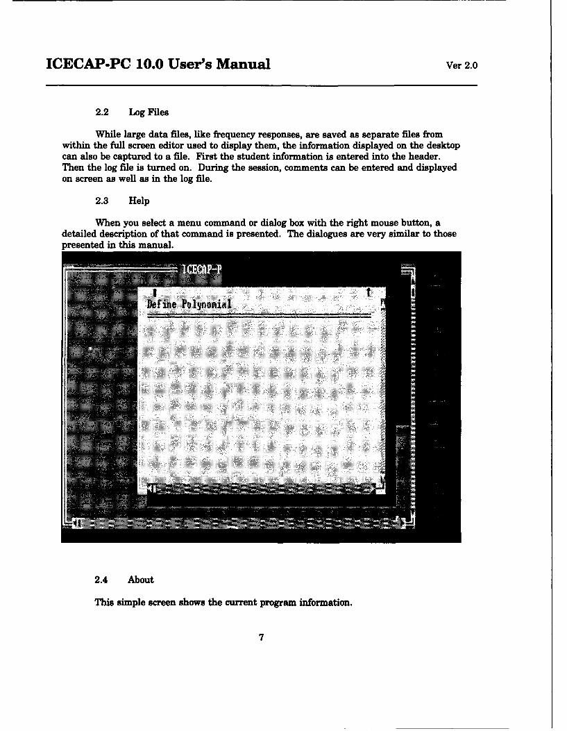
ICECAP-PC 10.0 User's Manual Ver 2.0
2.2 Log Files
While large data files, like frequency responses, are saved as separate fies fromwithin the full screen editor used to display them, the information displayed on the desktopcan also be captured to a file. First the student information is entered into the header.Then the log fie is turned on. During the session, comments can be entered and displayedon screen as well as in the log file.
2.3 Help
When you select a menu command or dialog box with the right mouse button, adetailed description of that command is presented. The dialogues are very similar to thosepresented in this manual.
D f n :••: F• iiPolynomial:i: i: :::i . :i::• :
2.4 About
This simple screen shows the current program information.
7
ICECAP-PC 10.0 User's Manual Ver 2.0
2.5 View Options
The appearance of numerical output is completely formattable. Numbers can bedisplayed in fixed decimal, or scientific notation. The number of significant digitsdisplayed can also be adjusted. Note that the internal processing will still use maximumfloating point accuracy, regardless of the ntimber of digits displayed. 25 or 50 vertical linescan be displayed. T or J' can be displayed as the complex letter.
2.6 Shelling to DOS
If while working in ICECAP-PC, you need to briefly run another application, simplyshell to DOS, run the application, exit the application, and type 'EXIT' at the DOS promptto return to ICECAP-PC.
2.7 Exiting ICECAP-PC
The FILE - EXIT menu command or ALT-X is used to exit gracefully fromICECAP-PC. Information is always stored in the ICECAP-PC default session file to returnyou to this point in the next startup. If you desire to save this information in a userspecified file, use the UPDATE command.
8
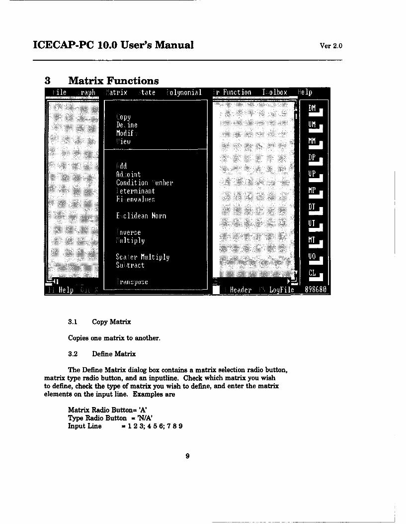
ICECAP-PC 10.0 User's Manual Ver 2.0
3 Matrix Functions
iI "I I. .. .
3.1 Copy Matrix
Copies one matrix to another.
3.2 Define Matrix
The Define Matrix dialog box contains a matrix selection radio button,matrix type radio button, and an inputine. Check which matrix you wishto define, check the type of matrix you wish to define, and enter the matrixelements on the input line. Examples are
Matrix Radio Button= 'AType Radio Button = 'N/AInput Line =12 3; 456; 78 9
9

ICECAP-PC 10.0 User's Manual Ver 2.0
gm S lub
. ........
Matrix Radio Button= 'B'Type Radio Button = 'Diag'Input Line = 1j2 3j4 5j6
Matrix Radio Button= 'C'Type Radio Button = 'Identity'Input Line = 3
3.3 Modify Matrix
The Modify Matrix dialog box contains a matrix selection radio button.Selection of a matrix results in a second dialog box on which to edit/redefineyour selected matrix. Check the type of matrix you wish to defineand modify or re-enter the matrix elements on the input line. Examples are
Matrix Radio Button= 'AType Radio Button = 'N/A'Input Line =12 3;4 56; 78 9
10
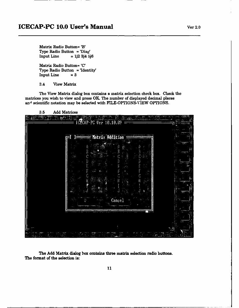
ICECAP-PC 10.0 User's Manual Ver 2.0
Matrix Radio Button= 'B'Type Radio Button = 'Diag'Input Line = 1j2 3j4 5j6
Matrix Radio Button= 'C'Type Radio Button = 'Identity'Input Line = 3
3.4 View Matrix
The View Matrix dialog box contains a matrix selection check box. Check thematrices you wish to view and press OK. The number of displayed decimal placesan'1 scientific notation may be selected with FILE-OPTIONS-VIEW OPTIONS.
3.5 Add Matrices
The Add Matrix dialog box contains three matrix selection radio buttons.
The format of the selection is:
11
ICECAP-PC 10.0 User's Manual Ver 2.0
A=B+C
Check the resultant radio button and the two operand radio buttons then pressOK to perform the operation. The resultant is displayed in the format chosenby the FILE-OPTIONS-VIEW OPTIONS setting.
3.6 Matrix Adjoint
The Matrix Adjoint dialog box contains two matrix selection check boxes.Check the matrices you wish to view and press OK. The format of the selectionis:
A = Adjoint(B)
The adjoint matrix can be calcuated in two ways. First it is the transpose of the cofactormatrix. Second it is the inverse times the determinant. ICECAP-PC uses the secondmethod. Select the resultant matrix on the left and the operand matrix on the right.The number of displayed decimal places and scientific notation may be selectedwith FILE-OPTIONS-VIEW OPTIONS.
3.7 Matrix Condition Number
The Matrix Condition Number dialog box contains a matrix selection check box.Check the matrix you wish to operate on and press OK. The format of the selectionis:
Condition Number(B)
The condition number is calculated as I IBI [ * I IB-I I.Select the resultant matrix on the left and the operand matrix on the right.The number of displayed decimal places and scientific notation may be selectedwith FILE-OPTIONS-VIEW OPTIONS.
3.8 Matrix Determinant
The Matrix Determinant dialog box contains two matrix selection check boxes.Check the matrices you wish to view and press OK. The format of the selectionis:
A = Determinant(B)
ICECAP-PC uses LU Decomposition to calculate the matrix determinant. Select theresultant matrix on the left and the operand matrix on the right. The number of displayeddecimal places and scientific notation may be selectedwith FILE-OPTIONS-VIEW OPTIONS.
12
ICECAP-PC 10.0 User's Manual Ver 2.0
3.9 Matrix Eigenvalues
The Matrix Eigenvalues dialog box contains a matrix selection check box.Check the matrix you wish to operate on and press OK The format of the selectionis:
Eigenvalues(B)
ICECAP-PC uses a three step process to calculate the eigenvalues. First, the matrix isbalances to produce an equivalent matrix containing the same eigenvalues but with a lowernorm. Second the matrix is converted to upper Hessenberg form using an orthogonalHouseholder transformation. Third, the eigenvalues are found using a double QR Shiftalgorithm. Select the resultant matrix on the left and the operand matrix on the right.The number of displayed decimal places and scientific notation may be selectedwith FILE-OPTIONS-VIEW OPTIONS.
3.10 Matrix Eigenvectors (The Modal Matrix)
The Matrix Eigenvectors dialog box contains a matrix selection check box.Check the matrix you wish to operate on and press OK. The format of the selectionis:
Eigenvectors(B)
Select the resultant matrix on the left and the operand matrix on the right.The number of displayed decimal places and scientific notation may be selectedwith FILE-OPTIONS-VIEW OPTIONS.
3.11 Matrix Euclidean Norm
The Matrix Euclidean Norm dialog box contains a matrix selection check box.Check the matrix you wish to operate on and press OK The format of the selectionis:
Euclidean Norm(B)
Select the resultant matrix on the left and the operand matrix on the right.The number of displayed decimal places and scientific notation may be selectedwith FILE-OPTIONS-VIEW OPTIONS.
3.12 Matrix Hermite Normal Form
The Matrix Hermite Normal Form dialog box contains a matrix selection check box.
Check the matrix you wish to operate on and press OK. The format of the selectionis:
13
ICECAP-PC 10.0 User's Manual Ver 2.0
Hermite Normal Form(B)
Select the resultant matrix on the left and the operand matrix on the right.The number of displayed decimal places and scientific notation may be selectedwith FILE-OPTIONS-VIEW OPTIONS.
3.13 Matrix Inverse
The Matrix Inverse dialog box contains two matrix selection check boxes.Check the matrices you wish to view and press OK. The format of the selectionis:
A = Inverse(B)
Select the resultant matrix on the left and the operand matrix on the right.The number of displayed decimal places and scientific notation may be selectedwith FILE-OPTIONS-VIEW OPTIONS.
3.14 Matrix Multiplication
The Multiply Matrix dialog box contains three matrix selection radio buttons.The format of the selection is:
A=BXC
Check the resultant radio button and the two operand radio buttons then pressOK to perform the operation. The resultant is displayed in the format chosenby the FILE-OPTIONS-VIEW OPTIONS setting.
3.15 Matrix Rank
The Matrix Rank dialog box contains a matrix selection check box.Check the matrix you wish to operate on and press OK. The format of the selectionis:
Rank(B)
Select the resultant matrix on the left and the operand matrix on the right.The number of displayed decimal places and scientific notation may be selectedwith FILE-OPTIONS-VIEW OPTIONS.
.topic MatrixScalerMultiplyff215Matrix Scaler Multiplication
The Matrix Scaler Multiply dialog box contains two matrix selection check boxes.Check the matrices you wish to view and press OK The format of the selectionis:
14
ICECAP-PC 10.0 User's Manual Ver 2.0
A = Scaler Multiple(B)
Select the resultant matrix on the left and the operand matrix on the right.The number of displayed decimal places and scientific notation may be selectedwith FILE-OPTIONS-VIEW OPTIONS.
3.16 Matrix Subtraction
The Subtract Matrix dialog box contains three matrix selection radio buttons.The format of the selection is:
A=B-C
Check the resultant radio button and the two operand radio buttons then pressOK to perform the operation. The resultant is displayed in the format chosenby the FILE-OPTIONS-VIEW OPTIONS setting.
3.17 Matrix Trace
The Matrix Trace dialog box contains two matrix selection check boxes.Check the matrices you wish to view and press OK. The format of the selectionis:
A = Trace(B)
Select the resultant matrix on the left and the operand matrix on the right.The number of displayed decimal places and scientific notation may be selectedwith FILE-OPTIONS-VIEW OPTIONS.
3.18 Matrix Transpose
The Matrix Transpose dialog box contains two matrix selection check boxes.Check the matrices you wish to view and press OK. The format of the selectionis:
A = Transpose(B)
Select the resultant matrix on the left and the operand matrix on the right.The number of displayed decimal places and scientific notation may be selectedwith FILE-OPTIONS-VIEW OPTIONS.
15

ICECAP-PC 10.0 User's Manual Ver 2.0
4 System Functions
iculator P3 Coutent P4 Heade
4.1 Defining Systems
4.2 Viewing Systems
4.3 Modifying
4.4 Copying
4.5 Controllability Matrix
The CNTABLE command determines if the system is controllable by generatingand finding the rank of the hermite form. The user is prompted for the plant matrix andthe control matrix.
4.6 Observability Matrix
16
ICECAP-PC 10.0 User's Manual Ver 2.0
The OBSABLE command determines if a system is observable by generating andfinding the rank of the hermite form. The user is prompted for the plant matrix and theobservation matrix.
4.7 Phase Variable Form
4.8 Observer Canonical Form
4.9 Observability Form
4.10 Controllability Form
4.11 Diagonal/Jordan Canonical Form
4.12 Tridiagonal Form
4.13 Hessenberg Form
4.14 Transform Domain
4.15 State Space to Transfer Function
The SSTOTF command generates the transfer function of a SISO state-spacesystem. The user specifies the matrix location of the system and the target transferfimction storage location. The specified system matrix should be in the form:
JAb
lcdI
4.16 System Analysis Graphics
4.16.1 Time Response
4.16.2 Frequency Response
4.16.3 Root Locus
4.16.4 Nichols Chart
4.16.5 Nyquist Plot
17
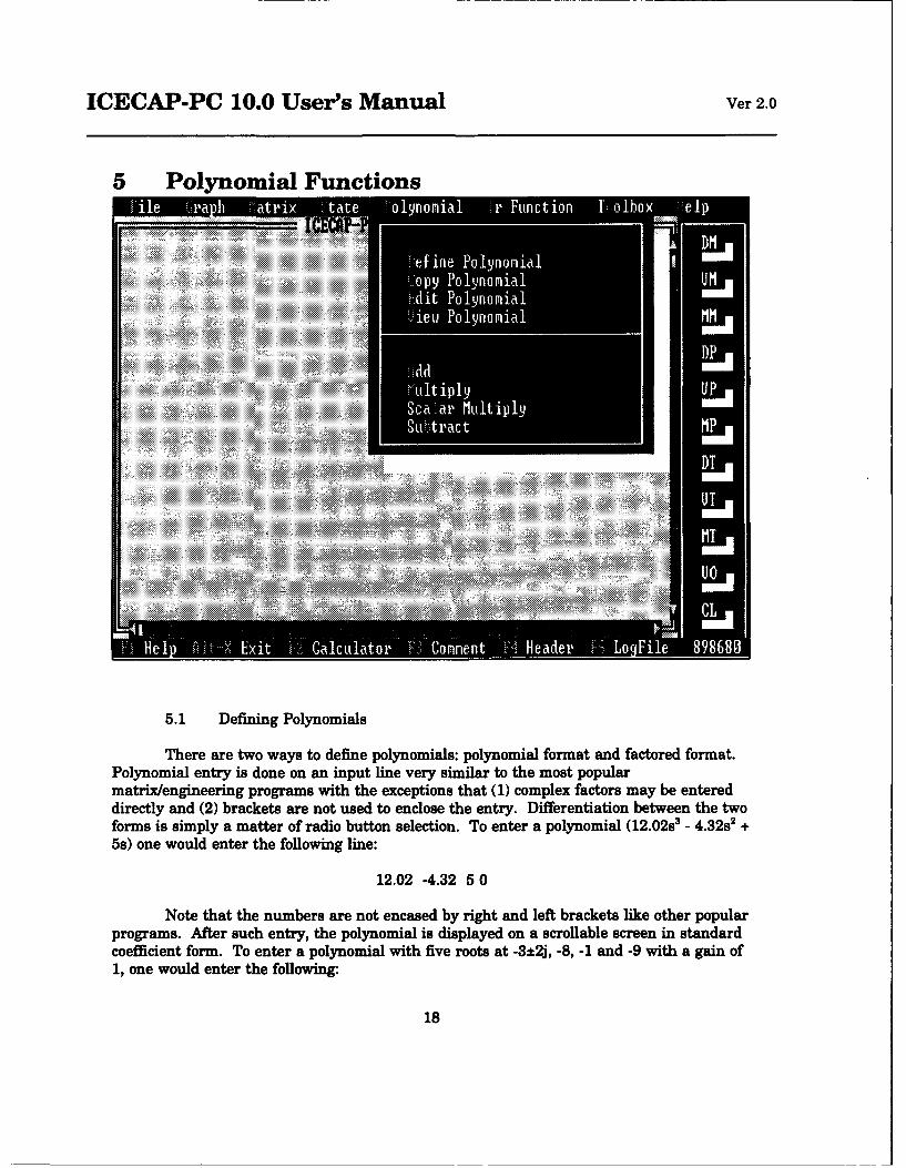
ICECAP-PC 10.0 User's Manual Ver 2.0
5 Polynomial Functions
I I
5.1 Defining Polynomials
There are two ways to define polynomials: polynomial format and factored format.Polynomial entry is done on an input line very similar to the most popularmatrix/engineering programs with the exceptions that (1) complex factors may be entereddirectly and (2) brackets are not used to enclose the entry. Differentiation between the twoforms is simply a matter of radio button selection. To enter a polynomial (12.02s3 - 4.3282 +5s) one would enter the following line:
12.02 -4.32 5 0
Note that the numbers are not encased by right and left brackets like other popularprograms. After such entry, the polynomial is displayed on a scrollable screen in standardcoefficient form. To enter a polynomial with five roots at -3*2j, -8, -1 and -9 with a gain of1, one would enter the following-
18

ICECAP-PC 10.0 User's Manual Ver 2.0
mam
-3j2 -8 -1 -9
Note the direct entry of the single complex variable. The entry of complex roots isalways done with an i or j preceding the complex element with no spaces allowed. Theentry of spaces in a complex number is taken to be a second root at an imaginary location.The entry of the complex conjugate is done automatically by the computer. Manual entryof the complex conjugate is allowed and will be detected by the program. After such entry,the polynomial is displayed on a scrollable screen in either factored form or in list formshowing the gain and root locations of the polynomial as selected by the user.
5.2 Viewing Polynomials
Select all polynomials desired to be viewed and a format for displaying them.
5.3 Copying
Select the polynomial to be copied, and then the storage location to which to copy itto.
19

ICECAP-PC 10.0 User's Manual Ver 2.0
5.4 Adding
Select the radio buttons for the two polynomials you want added together and thelocation for the result. If you desire, you may add POLYA and POLYA together and storethe result in POLYA.
5.5 Subtracting
Select the radio buttons for the two polynomials you want subtracted, in the ordershown--left minus right--and the location for the result. If you desire, you may subtractPOLYA from POLYA and store the result in POLYA.
5.6 Multiplying
Select the radio buttons for the two polynomials you want multiplied and thelocation for the result. If you desire, you may multiply POLYA and POLYA and store theresult in POLYA.
5.7 Scalar Multiplying
Select the polynomial you want to multiply by a gain factor, enter the gain factorvalue, and select a location for the result to be stored. Negative gain factors are allowed.
20
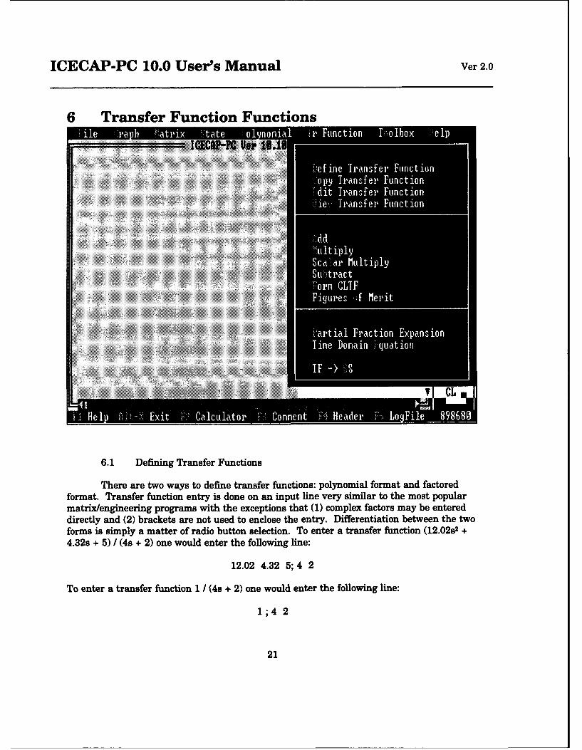
ICECAP-PC 10.0 User's Manual Ver 2.0
6 Transfer Function Functions
Itutip'11ly f.111
Sc .a ! ......
uuuli,.uIinb:tr1111
6.1 Defining Transfer Functions
There are two ways to define transfer functions: polynomial format and factoredformat. Transfer function entry is done on an input line very similar to the most popularmatrix/engineering programs with the exceptions that (1) complex factors may be entereddirectly and (2) brackets are not used to enclose the entry. Differentiation between the twoforms is simply a matter of radio button selection. To enter a transfer function (12.02s2 +
4.32s + 5) / (4s + 2) one would enter the following line:
12.02 4.32 5; 4 2
To enter a transfer function 1 / (4s + 2) one would enter the following line:
1;4 2
21
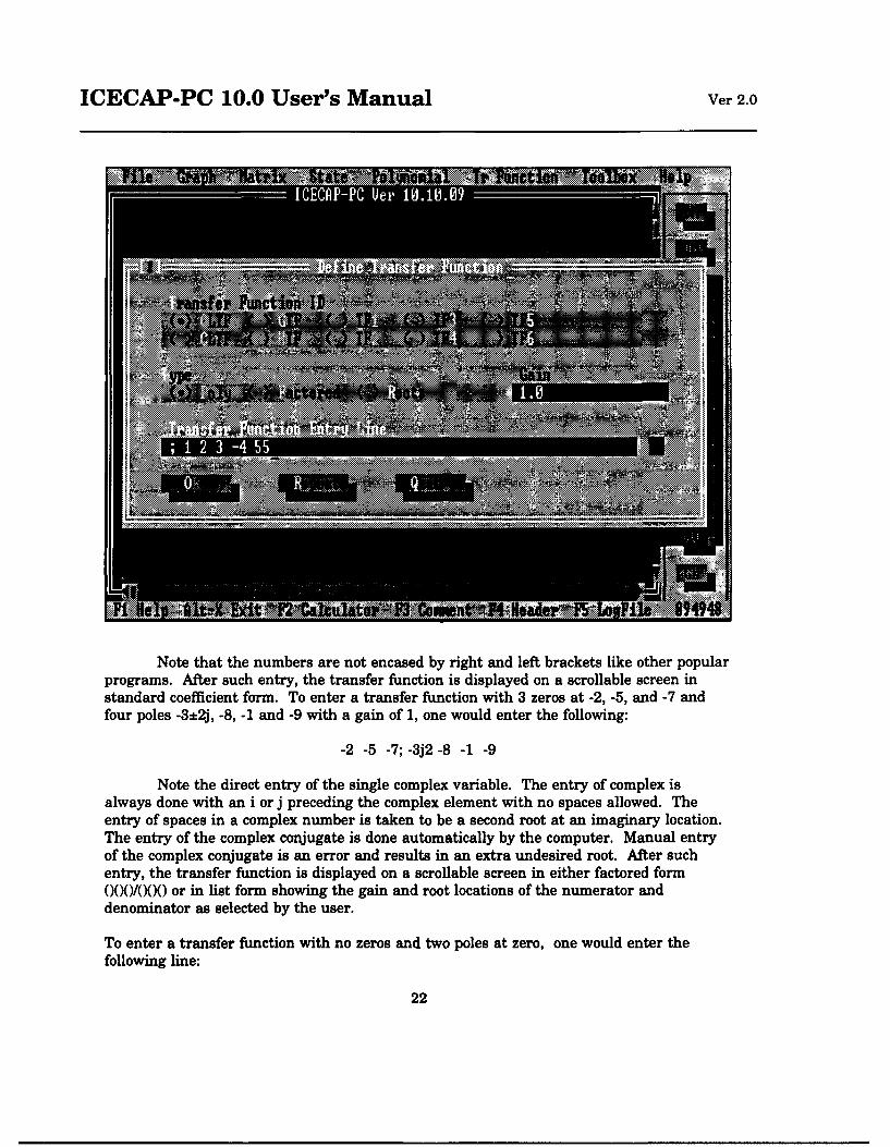
ICECAP-PC 10.0 User's Manual Ver 2.0
..... .....-
I..........
•" ::}:': "•: ::::•" ":: .•
Note that the numbers are not encased by right and left brackets like other popularprograms. After such entry, the transfer function is displayed on a scrollable screen instandard coefficient form. To enter a transfer function with 3 zeros at -2, -5, and -7 andfour poles -3*2j, -8, -1 and -9 with a gain of 1, one would enter the following:
-2 -5 -7; -3j2 -8 -1 -9
Note the direct entry of the single complex variable. The entry of complex isalways done with an i or j preceding the complex element with no spaces allowed. Theentry of spaces in a complex number is taken to be a second root at an imaginary location.The entry of the complex conjugate is done automatically by the computer. Manual entryof the complex conjugate is an error and results in an extra undesired root. After suchentry, the transfer function is displayed on a scrollable screen in either factored form000/(X)0 or in list form showing the gain and root locations of the numerator anddenominator as selected by the user.
To enter a transfer function with no zeros and two poles at zero, one would enter thefollowing line:
22
ICECAP-PC 10.0 User's Manual Ver 2.0
;00
6.2 Viewing Transfer Functions
Select all transfer functions desired to be viewed and a format for displaying them.
6.3 Copying
Select the transfer function to be copied, and then the transfer function location towhich to copy it to.
6.4 Adding
Select the radio buttons for the two transfer functions you want added together andthe location for the result. If you desire, you may add TF1 and TF1 together and store theresult in TF1.
6.5 Subtracting
Select the radio buttons for the two transfer functions you want subtracted, in theorder shown--left minus right-and the location for the result. If you desire, you maysubtract TF1 from TF1 and store the result in TF1.
6.6 Multiplying
Select the radio buttons for the two transfer functions you want multiplied and thelocation for the result. If you desire, you may multiply TF1 and TF1 and store the result inTF1.
6.7 Scalar Multiplying
Select the transfer function you want to multiply by a gain factor, enter the gainfactor value, and select a location for the result to be stored. Negative gain factors areallowed.
6.8 Form CLTF
The FORM command is used to produce the CLTF from either the OLTF or acombination of GFT and HFT. The formulas for producing the CLTF is as follows:
CLTF = (GAIN*GFT)/(1+GAIN*GFT*HFTr)CLTF = (GAIN * OLTF) / ( 1 + GAIN * OLTF)CLTF = GFT + HIFT ( In Parallel )
The FORM command will also form the OLTF from the GFT and the HTF. Theformula for that operation is:
23
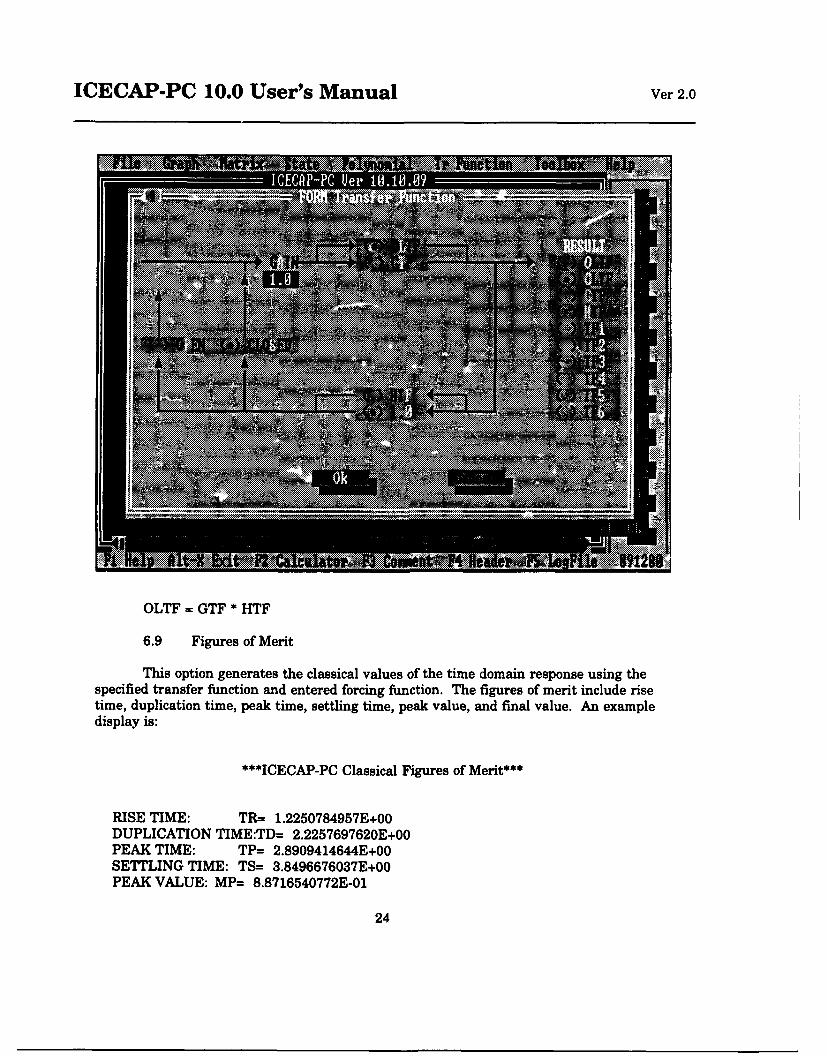
ICECAP-PC 10.0 User's Manual Ver 2.0
OLTF GTF * HTF
6.9 Figures of Merit
This option generates the classical values of the time domain response using thespecified transfer function and entered forcing function. The figures of merit include risetime, duplication time, peak time, settling time, peak value, and final value. An exampledisplay is:
***ICECAP-PC Classical Figures of Merit***
RISE TIME: TR= 1.2250784957E+00DUPLICATION TIME:TD= 2.2257697620E+00PEAK TIME: TP= 2.8909414644E+00SETTLING TIME: TS= 3.8496676037E+00PEAK VALUE: MP= 8.8716540772E-o01
24
ICECAP PC 10.0 User's Manual Ver 2.0
FINAL VALUE: FV= 8.4761565716E-01
6.10 Time Equation
This option displays the time-domain continuous or discrete equation terms for thespecified transfer function and input (for the continuous case using the Heavisidepartial-fraction expansion method). An example is:
*** Output Equation Terms for Specified Input ***
c(t)=
-0.203449 exp(-4.319476 t) sin(3.434581 t + 175.463663)
-1.697083 exp(-1.180524 t) sin(1.181357 t + 29.338792)
0.847616
6.11 Partial Fraction Expansion
This option displays the partial fraction coefficients of the specified transferfunction with entered forcing function. The polar representations are also displayed.Available forcing function functions are impulse, step, ramp, pulse and sinusoidal. Forexample, a resulting display is:
***ICECAP-PC Partial Fraction Expansion***
CLTF
Numerator Coefficient Corresponding Pole Order
-8.04553E-03 + j-1.01406E-01 -4.31948E+00 + j 3.43458E+00 1-8.04553E-03 + j 1.01406E-01 -4.31948E+00 + j -3.43458E+00 1-4.15762E-01 + j 7.39706E-01 -1.18052E+00 + j 1.18136E+00 1-4.15762E-01 + j-7.39706E-01 -1.18052E+00 + j -1.18136E+00 18.47616E-01 + j 0.OOOOOE+00 0.OOOOOE+00 + j 0.OOOOOE+00 1
6.12 Transform Domain
This command permits a specific domain transfer function to be transformed intothe desired domain using the following transformations:
z to s Inverse Z transformation INZ (impulse)s to z Tustin transformation SZJTUSTIP (bilinear)w' to z bilinear transformation - WPZ(BILIN
25
ICECAP-PC 10.0 User's Manual Ver 2.0
w to z bilinear transformation - WZ/BILINs to z z-transform - ZTRANS (impulse)z to w' bilinear transformation - ZWP/BILINz to w bilinear transformation - ZW/BILIN
The user selects one of the above transformations and the specific transfer functionhe desires to transform. The result is placed into the selected transfer function's data file,overwriting the previous domain's data.
The technique to perform the INZ and ZTRANS symbolic transformations uses thepartial fraction expansion approach.
Note that the ZTRANS exact Z transformation can transform an s-plane transferfunction with a root of maximum multiplicity 10! When using ZTRAN, ICECAP will askyou if you want to add a Zero-order hold (ZOH). The INZ can transform a z-plane transferfunction with a root of maximum multiplicity 2! The other transforms employ the standardbilinear transformation.
6.13 Transfer Function to State Space
The TFTOSS command generates the state space representation of a system usingthe phase variable technique. It is the inverse of the SSTOTF command.
6.14 Transfer Function Analysis Graphics
6.14.1 Time Response
This option lists the time response of a specified s-plane transfer function with enteredforcing function and time interval. The available forcing functions are impulse, step, ramp,pulse and sinusoidal.
Plotting Bounds: Users can enter their own plotting bounds as requested by the system.
Grid: The user can request a background (linear and log for bode plots or general plots).
6.14.2 Frequency Response
Given a continuous or discrete transfer function, the frequency response procedurecalculates the magnitude and phase angle for a range of frequencies. The procedure givesthe user a choice of units for frequency (radians/second or hertz), magnitude (normalizedunits or decibels), and phase angle (radians or degrees). A log frequency or linearfrequency range can be selected. If log frequency is selected, the user is requested to enterthe "number of cycles" and the "power of the starting frequency ", i.e. to begin at afrequency of 0.01, you want 10', so enter -2 as the starting power. The user can also selectlinear frequency (omega). A specific step size (del) and range can be entered for
26
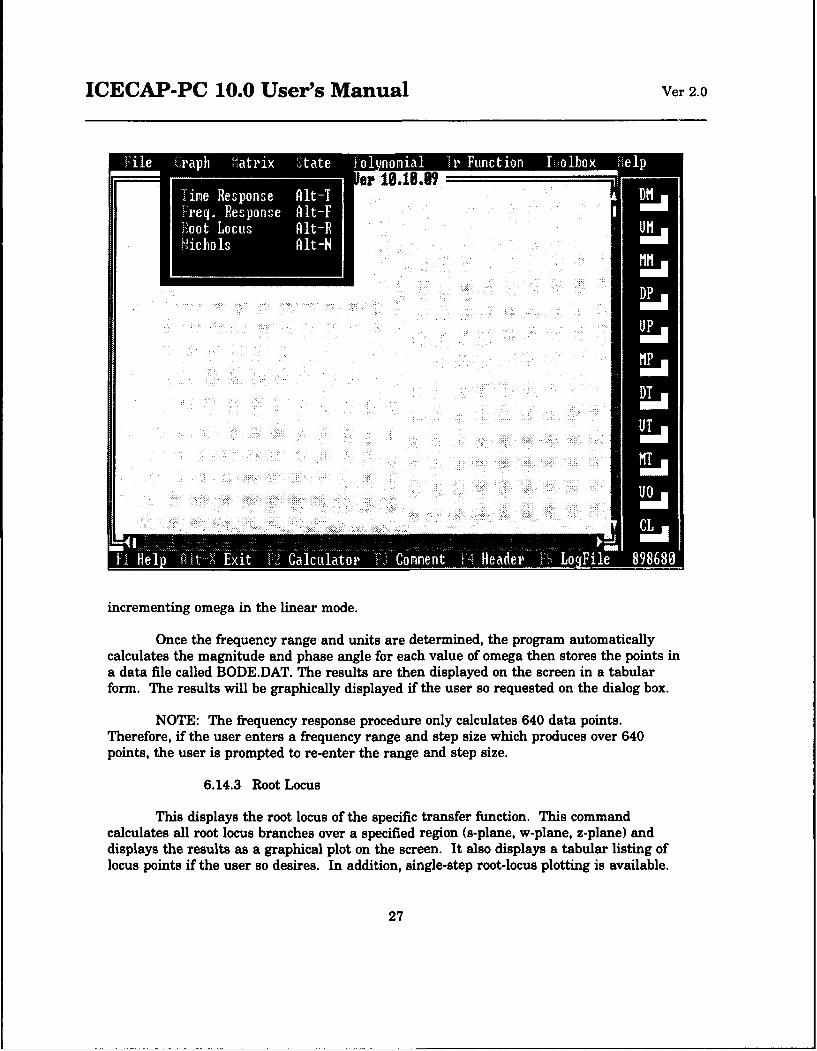
ICECAP-PC 10.0 User's Manual Ver 2.0
-- .1 8.8./
incrementing omega in the linear mode.
Once the frequency range and units are determined, the program automaticallycalculates the magnitude and phase angle for each value of omega then stores the points ina data file called BODE.DAT. The results are then displayed on the screen in a tabularform. The results will be graphically displayed if the user so requested on the dialog box.
NOTE: The frequency response procedure only calculates 640 data points.Therefore, if the user enters a frequency range and step size which produces over 640points, the user is prompted to re-enter the range and step size.
6.14.3 Root Locus
This displays the root locus of the specific transfer function. This commandcalculates all root locus branches over a specified region (s-plane, w-plane, z-plane) anddisplays the results as a graphical plot on the screen. It also displays a tabular listing oflocus points if the user so desires. In addition, single-step root-locus plotting is available.
27
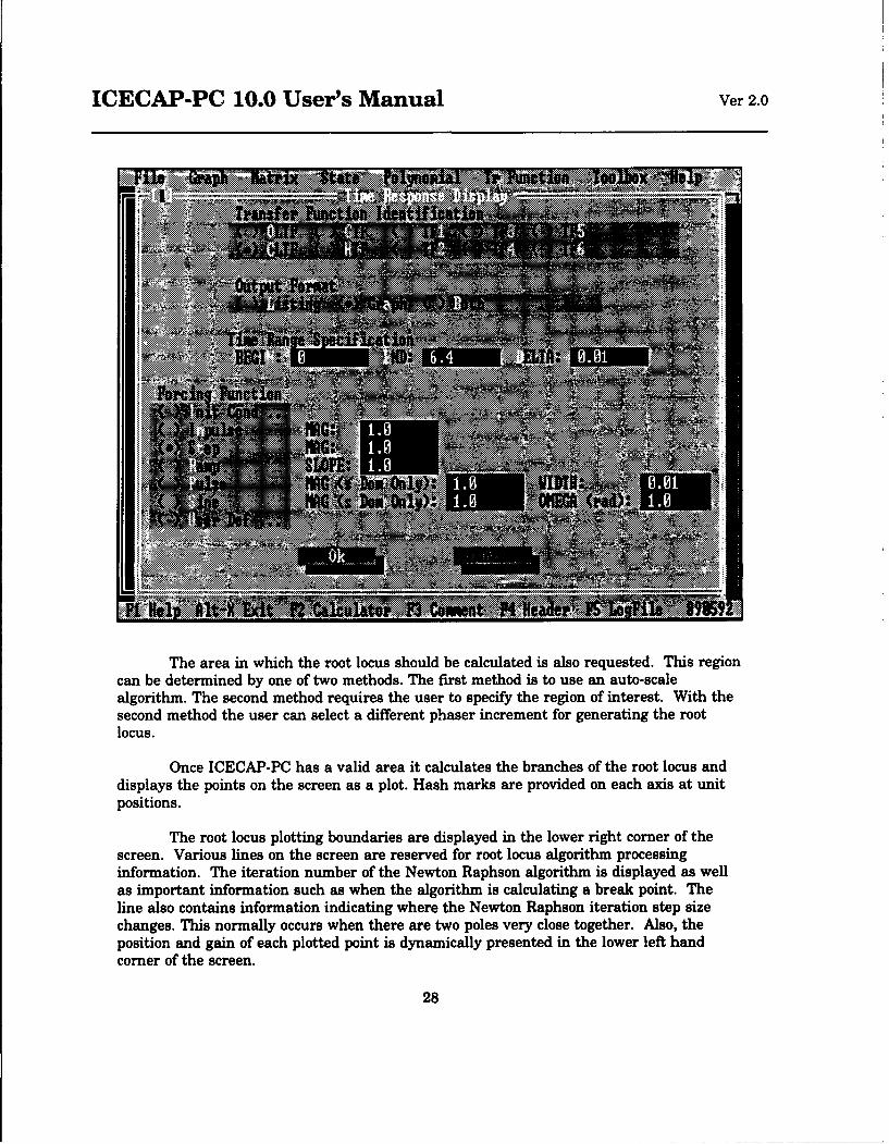
ICECAP-PC 10.0 User's Manual Ver 2.0
The area in which the root locus should be calculated is also requested. This regioncan be determined by one of two methods. The first method is to use an auto-scalealgorithm. The second method requires the user to specify the region of interest. With thesecond method the user can select a different phaser increment for generating the rootlocus.
Once ICECAP-PC has a valid area it calculates the branches of the root locus anddisplays the points on the screen as a plot. Hash marks are provided on each axis at unitpositions.
The root locus plotting boundaries are displayed in the lower right corner of thescreen. Various lines on the screen are reserved for root locus algorithm processinginformation. The iteration number of the Newton Raphson algorithm is displayed as wellas important information such as when the algorithm is calculating a break point. Theline also contains information indicating where the Newton Raphson iteration step sizechanges. This normally occurs when there are two poles very close together. Also, theposition and gain of each plotted point is dynamically presented in the lower left handcorner of the screen.
28
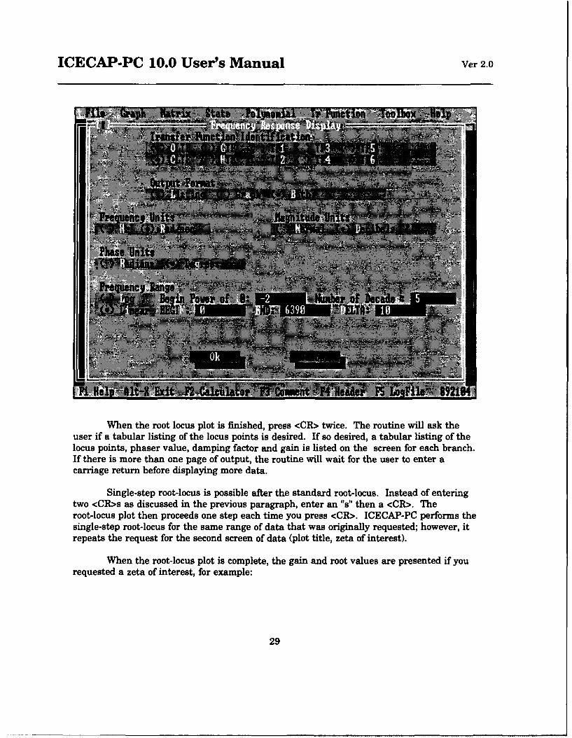
ICECAP-PC 10.0 User's Manual Ver 2.0
Ng:0
When the root locus plot is finished, press <CR> twice. The routine will ask theuser if a tabular listing of the locus points is desired. If so desired, a tabular listing of thelocus points, phaser value, damping factor and gain is listed on the screen for each branch.If there is more than one page of output, the routine will wait for the user to enter acarriage return before displaying more data.
Single-step root-locus is possible after the standard root-locus. Instead of enteringtwo <CR>s as discussed in the previous paragraph, enter an "s" then a <CR>. Theroot-locus plot then proceeds one step each time you press <CR>. ICECAP-PC performs thesingle-step root-locus for the same range of data that was originally requested; however, itrepeats the request for the second screen of data (plot title, zeta of interest).
When the root-locus plot is complete, the gain and root values are presented if yourequested a zeta of interest, for example:
29
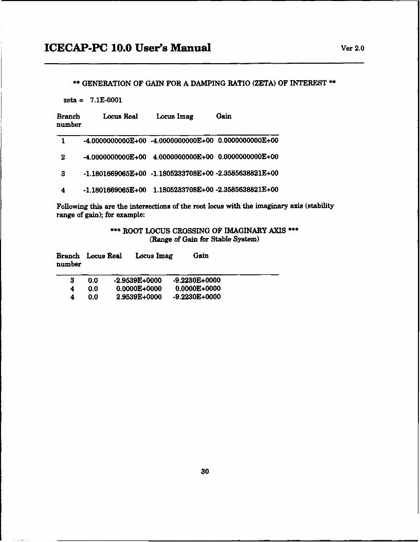
ICECAP-PC 10.0 User's Manual Ver 2.0
** GENERATION OF GAIN FOR A DAMPING RATIO (ZETA) OF INTEREST **
zeta = 7.1E-0001
Branch Locus Real Locus Imag Gainnumber
1 -4.OOOOOOOOOOE+00 -4.OOOOOOOOOOE+00 O.OOOOOOOOOOE+00
2 -4.OOOOOOOOOOE+00 4.OOOOOOOOOOE+00 0.OOOOOOOOOOE+00
3 -1.1801669065E+00 -1.1805233708E+00 -2.3585638821E+00
4 -1.1801669065E+00 1.1805233708E+00 -2.3585638821E+00
Following this are the intersections of the root locus with the imaginary axis (stabilityrange of gain); for example:
*** ROOT LOCUS CROSSING OF IMAGINARY AXIS ***
(Range of Gain for Stable System)
Branch Locus Real Locus Imag Gainnumber
3 0.0 -2.9539E+0000 -9.2230E+00004 0.0 0.OOOOE+0000 0.OOOOE+00004 0.0 2.9539E+0000 -9.2230E+0000
30

ICECAP-PC 10.0 User's Manual Ver 2.0
FIGURE 5
31
ICECAP-PC 10.0 User's Manual Ver 2.0
6.14.4 Nichols Chart
Constant Mp curves and constant angle curves for the closed loop are alsopresented over the following ranges:
Mp in db 13,8,5,3,2,1,0,-1,-2,-3,-5,-8, -13,-22;angle in degrees -340,-320,-300,-280,-260,-240,-220,-200,
-160,-140,-120,-100,-80,-60,-40,-20.
Displaying the constant Mp and angle curves is controlled by the SWITCH command (theconstant Mp curves default to "on", the constant angle curves default to "off") (Fig. 4).
A Nichols chart display of the data in the BODE.DAT file as generated using theFrequency Response routine can be requested. Constant Mp curves and constant anglecurves for the closed loop are also presented over the ranges as listed above.
Nyquist Plot
This option graphically displays the polar plot of the entered transfer functionalong with the associated gain margin and phase margin. Also, an optional plot title isrequested. See example display of Fig. 6.
32
ICECAP-PC 10.0 User's Manual Ver 2.0
FIGURE 6
33
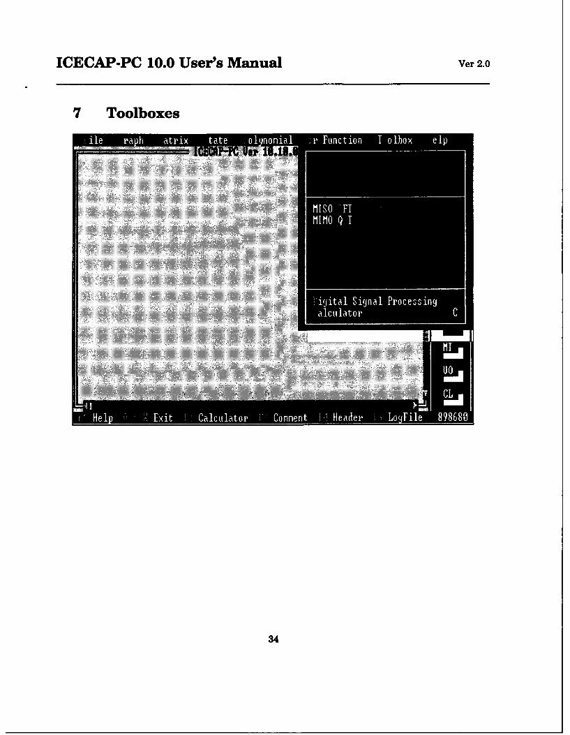
ICECAP-PC 10.0 User's Manual Ver 2.0
7 Toolboxes
I Io I
iiii~igta Signall Processingiiiii£•WlaQt-I -•-
34
ICECAP-PC 10.0 User's Manual Ver 2.0
APPENDIX A. PRINTING
All printing of graphics can be accomplished by using a screen-dump package.
EGA terminals should use "EGADMP" (Part of "CHART 4" package). We distributeEGADMP configured to work with an EPSON printer. For laser printers we distributeLJEGADMP, which is configured for an HP. EGADMP can be reconfigured for otherprinters.
CGA terminals should use "GRAPHICS" under MS-DOS.
For VGA terminals use of a commercial package such as "GRAPPLUS" issuggested. The proper graphics and printer drivers must be installed as prescribed by eachof those individual packages. If you have a VGA interface and do not own a commercialscreen dump program, reprogramming your monitor as an EGA terminal will usuallypermit the EGADMP routine to execute properly.
35
ICECAP-PC 10.0 User's Manual Ver 2.0
APPENDIX B. IF PROBLEMS ARE ENCOUNTERED
The following is a brief list of actions to take when problems are encounteredduring execution of ICECAP-PC.
6.1 Errors During Initialization
Make sure all files required by the ICECAP-PC reside in the same disk directory asICECAP-PC. Attempt to re-execute the program.
6.2 A "trashy" Title Slide Appears
1. Attempt to re-execute the program.
6.3 Graphics Display Problems
1. Since ICECAP-PC determines the type of graphic terminal interface (CGA, EGA,VGA,...) before plotting, the interface should be checked for proper switch selection(reference Turbo Pascal Graph Unit).
2. If the colors that are presented are not desired, change source code in
ICECAP-PC graphics modules. (reference Turbo Pascal Graph Unit).
3. Try to obtain a .BGI file from Borland to drive your unique monitor.
6.4 System Hang Up
1. Read the documentation that was shipped with the new DPMI drivers.
6.5 Problem Report Form
Attached is a blank problem report form. Please copy and submit comments asappropriate to the indicated address or use electronic mail.
36
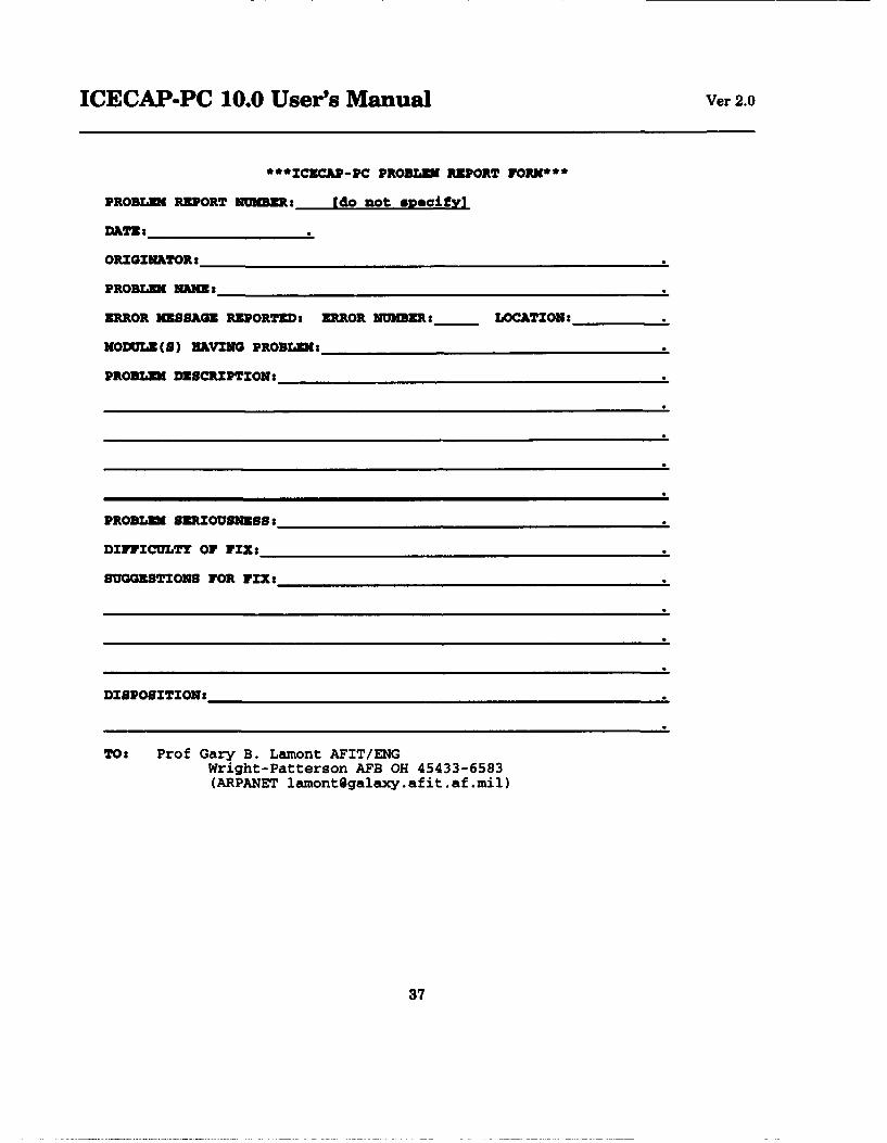
ICECAP-PC 10.0 User's Manual Ver 2.0
***XCZCIA1-1C PROBLDI REPORT FORK***
PROBLfh REPORT NUMB=: (do noat siDecify]
DATE: __ __ _
ORIOINATOR:
PRODLUI 3MM:
EDROR =SSAGE DEPORTED: EDROR NUMBE:___ LOCATION:_____
MODULE(S) HAVING PROBLDI:______ ____________
PROBLUE DESCRIPTION 2
PROBLEI SERIOUSNESS:_____________________
DIFFICULTY 01 VIZ:______________________
SUGGESTIONS FOR VIZ:____________________
DISPOSITION:
TO: Prof Gary B. Lamonit AFIT/ENGWright-Patterson AFB OH 45433-6583(ARPANET lamorit~galaxy.af it .af.mil)
37
ICECAP-PC 10.0 User's Manual Ver 2.0
APPENDIX C. Theoretical Background of ICECAP-PC Algorithms
(in progress)
38

ICECAP-PC 10.0 User's Manual Ver 2.0
APPENDIX D. Basic Continuous Compensation Toolbox
This toolbox provides the student several template-style filters to usefor control. The templates include Lead-Lag, Butterworth, and Chebychevfilters. The student specifies the performance requirements and the plant,and the toolbox generates the proper filter parameters.
39
ICECAP-PC 10.0 User's Manual Ver 2.0
APPENDIX E. Nonlinear Modelling Toolbox
40
ICECAP-PC 10.0 User's Manual Ver 2.0
APPENDIX F. System Build Toolbox
41
ICECAP-PC 10.0 User's Manual Ver 2.0
APPENDIX G. Linear Quadratic Regulator/Gaussian/Compensator Toolbox
This toolbox provides the student with an LQR when he provides theplant and Q and R parameters. It also will provide an LQG estimator andthe combination of the two into an LQ Compensator system.
The LQRCONT command solves the linear quadratic regulatorproblem by generating the solution to the Riccati equation (uses eigenvaluedecomposition), determining the constant control gain and generating theclosed-loop eigenvalues. The user is prompted for the plant, control andweighting matrices.
42
ICECAP-PC 10.0 User's Manual Ver 2.0
APPENDIX H. Kalman Filtering Toolbox
This toolbox is a port of Dr Maybeck's Matlab M-File program suitecalled KFEval. It allows the student to design Kalman filters.
43

ICECAP-PC 10.0 User's Manual Ver 2.0
APPENDIX I. H Infinite Toolbox
This toolbox allows the students to design controllers using the HInfinite method.
44
ICECAP-PC 10.0 User's Manual Ver 2.0
APPENDIX J. Eigenstructure Assignment Toolbox
This toolbox provides a matrix method for designing controllers.
45
ICECAP-PC 10.0 User's Manual Ver 2.0
APPENDIX K. Multi-Porter Method Toolbox
This toolbox provides a specific type of Eigenstructure Assignmentcalled the Multi-Porter Method.
46

ICECAP-PC 10.0 User's Manual Ver 2.0
APPENDIX L. Digital Signal Processing Toolbox
(Major Development by D. Gelopulos, Valparaiso University)
A set of Pascal programs have been incorporated that provideelementary digital signal processing analysis and synthesis functions. Themain DSP menu ICECAP provides looks like:
DEMOS DFT FF1: FOURSERHELP
3.1.4.1 DEMOS
The DEMOS command permits the following variety ofdemonstrations:
1) Convolution2) Fourier Series3) Phase4) Aliasing5) DFT test data generation
The user is initially requested to enter anumber corresponding to one of these demonstrations, which are describedin the following paragraphs.
"Convolution Demonstration"
This program asks the user to specify a discrete unit pulse response and aninput sequence. The program displays the response to each sample in theinput sequence and shows how it combines with the response to all previousinput samples to form the system response. The user may also request arecord of the experiment which will be recorded in a disk file in the form ofa convolution summation table. The user may name a file for saving thecalculation of the convolution with respect to the response to each inputsample as well as the total system response.
"Fourier Series Demonstration"
47
ICECAP-PC 10.0 User's Manual Ver 2.0
This Program Demonstrates The ability of the Fourier series to represent asquare wave. This program displays a square wave, and a truncated,Fourier series of the wave. The square wave (red), its Fourier series(yellow) and the previously exhibited series (green) can all be displayedtogether for comparison. To see "Gibbs" phenomenon, use high resolutiongraphics and more than 50 harmonics. The user enters the number ofharmonics he wishes to include after each display is produced. The usermay also interrupt the display at any time to enter the harmonic number.Enter a "0" to terminate the execution.
"Phase Demonstration"
This demo generates a complex phasor rotation and the associatedprojection of its real and imaginary parts. The user enters four phasors (amplitude and phase ), one at a time using amplitudes between 10 and 110.
"Aliasing Demonstration"
This Program Demonstrates The Aliasing of samples of a sinusoidal signal.The user enters a frequency. The program generates the alias signals, oneat a time. The user must identify how many periods of a sinusoid to display,and how frequently it is sampled. The program displays the sine wave andan alias sinusoid which has the same values at sample times. Each timethe program is re-run the next higher alias frequency is shown. The displayis interrupted at each sample time for emphasis. To Terminate theprogram, press "E" at the END of a display.
"DFT Test Data Generation:"
The following Pascal program generates the dft test data. To run theprogram as is and generate the data as is, just choose option 5 from theDSP DEMO menu. However, if you want to generate a different set of testdata, you could develop your own program based on this example. Todevelop your own program would require writing it and compiling andrunning it outside of ICECAP. Then run ICECAP and whenever it requestsa filename for the DFT routines, enter the name of the file your programcreated.
48

ICECAP-PC 10.0 User's Manual Ver 2.0
program dft-data.generation;
var j, n: integer; x, wit, w2t, dwlt, dw2t : real; out: text;
BeginClearscreen;Writeln(' Please input desired DFT data file name ');Reset(input);Read(filename);Assign( out, filename);Rewrite( out );Writeln( out, 'DFT test data: 5 sin(4 wo t) + 5 cos( 40 wo t )');Writeln( out);Writeln( out);n := 128;wit := 0;w2t := 0;dwlt := 8 * Pi / n;dw2t := 80 * pi / n;Forj := Ito n do
Beginx :=5*(sin(wlt)+cos(w2t));wlt := wit + dwit;w2t := w2t + dw2t;Writeln( out, (j-1):5, x:12:4)
End;Close( out );End. (end of program dfLdatageneration}
3.1.4.2 FFT: CALCULATION OF FAST FOURIER TRANSFORMCOEFFICIENTS
The samples to be Fourier transformed ( to have the D.F.T. evaluated), should be listed in a sequential file, one sample per line. The first lineshould contain a one-line heading and the next two lines may haveanything. The first sample should appear in line four.
To do an inverse D.F.T., the data file should have the followingformat: First line of the file should contain a one-line heading. Lines 2 & 3
49
ICECAP-PC 10.0 User's Manual Ver 2.0
can have anything. Line 4 has the real and imaginary part of the firstspectrum point. Line 5 has the next point, etc.
Line numbers may precede a data point, and will be ignored if the fileis declared by the user as "numbered" when asked by the program. Thenumber of data points must be a power of two. Do NOT use a blank for avalue of zero!
Data sets are limited to 4096 in length. A sample data file can begenerated under DSP DEMO.
3.1.4.3 DFT: GENERATION OF D.F.T. COEFFICIENTS FOR SMALLDATA
SETS
The form of the sequential data file is the same as that for the FFT.
Data sets are limited to 1024 in length because F.F.T. is NOTimplemented in this program. It is intended to be transparent code foracademic size problems. The DSP DEMOS option 5 can be used to generatea test file.
3.1.4.4 SERIES: CALCULATION OF FOURIER COEFFICIENTS
This procedure is programmed by the user to evaluate the wave forwhich the Fourier series is sought at "time = TIME". The general examplecalculates and graphically presents the series of a square wave whichequals "1" for the first half period and "0" for the last half.
This program is interactive. It is necessary to reprogram a functionto calculate the wave of interest. The user enters the period of the wave aswell as the number of harmonics to be calculated. If you wish to save theresponse, enter a file name. If a file name is not entered, the Fourier seriescoefficients are listed in two forms: the trigonometric coefficients with An(cosine) and Bn (sine), and then the polar form of the phasors with "sine" asreference. The nominal time step selected by the user is trimmed so thatan integer number of time steps fits exactly into one period.
50
Appendix D ICECAP-PC Programmer's Manual

ICECAP- PCVersion 10.0 - MS-DOS
Interactive Control Engineering Computer Analysis Packagefor the Personal Computer
Programmer's Manual v 1.0
Professor Gary B. LamontDepartment of Electrical and Computer Engineering
School of EngineeringAir Force Institute of Technology
Wright-Patterson AFBDayton, Ohio 45433-6583
cooperative copyrighted 1992
PREFACE
WELCOME to the Programmer's Manual for ICECAP-4C. ICECAP-PC is an ongoing development ofa public domain computer-aided design (CAD) package for students, faculty and practitioners of controlengineering and digital signal processing with special emphasis on education. Source code andexecutable files are available. If you are interested in adding additional code or have suggestions forimprovement please contact:
Professor Gary B. LamontDepartment of Electrical and Computer Engineering
School of EngineeringAir Force Institute of Technology
Wright-Patterson AFB OH 45433-6583(513) 255-3450
(ARPANET [email protected])
cooperative copyright (C) 1985, 1986, 1987, 1988, 1989, 1990,1991,1992 Gary B. Lamont, Susan K.Mashiko, Gary C. Tarczynski, D. Gelopulos, Paul A. Moore, Wayne E. Bell, Vincent M. Parisi, FredTrevino, Mark W. Schiller, Ken A. Crosby
This public domain CAD package is intended for the main purpose of education and thus theexecutable code can be distributed freely. Any use of the package in support of written publicationsshould be indicated as a reference. Changes to the public domain source code that improve and extendits capabilities are appreciated, however, all suggested changes should be communicated to the authorsfor updating and dissemination of the next official version.
Permission to use, copy and distribute this software for educational purposes without fee is herebygranted provided that the copyright notice and this permission notice appear on all copies. Permissionto modify the software is granted, but not the right to distribute the modified code. All modificationsare to be distributed as changes to released versions by AFIT.
ICECAP-PC is written in Borland'st Turbo PASCAL 6.0 and TurboVision, both of which are registeredtrademarks and copyrighted by Borland International, Inc. 1800 Green Hills Road, P.O. Box 660001,Scotts Valley, CA 95067-0001. The .BGI files distributed with our package are released to publicaccess by Borland.
All references to MS-DOS in this document refer to Microsoft-DOS which is a registered trademarkand copyrighted by MicroSoftl.. Corporation.
SYSTEM REQUIREMENTS
ICECAP-PC is designed to work on MS-DOSt 80286/80386/80486 computers with a minimum of 640KB of RAM and 5MB of hard disk space. ICECAP-PC supports all graphics terminals includingHerculest., EGA and VGA. Operation is greatly enhanced with expanded memory and a math co-processor. Installation of ICECAP-PC and its QFT Toolbox is done automatically with a providedinstall procedure (see ICECAP-PC manual).
Edited By: Gary B. Lamont , Wayne E. Bell, and Fred Trevino; 1992

Table of Contents
1 Introduction ........................................................ 2
2 The Programmer's Guide .............................................. 3
ICECAP-PC Programmer's Manual Ver 1.0
1 Introduction
ICECAP-PC is fully object-oriented. In order to call one of its internal routines, one needonly do the following:
(1) Fill the global record associated with the desired routine with the appropriate data.(2) Send a message to the DeskTop invoking the desired object.
The message is formatted like this:
Message(DeskTop, evBroadCast, brDesiredRoutineName, nil);
The brDesiredRoutineName is the only variable element in this message. All the br commandsand their associated routines are found in Chapter 2. If a routine has a global record for passingparameters associated with it, the global record is also listed along with the routines. Most of theglobal records further have associated with them transitional routines. These transitional routinesmake it easier to copy information from the global record of one routine to that of another. Theymust only be used when one is doing plots with multiple responses on the same plot. Typically,one must only call the main plot routine. For example, if one is currently working with thefrequency response routine and wants to call a graphics plot of the response, one would summonthe FreqDisplay routine with the following message:
Message(DeskTop, evBroadCast, brFreqDisplay, nil);
It is this ability to send anonymous messges to the Desktop, that makes object-oriented code soexpandable. Future development will include expanding this macro-type language support for ourcode, making it more convenient and flexible for future programmers to use our package as amacro language or 4GL.
2
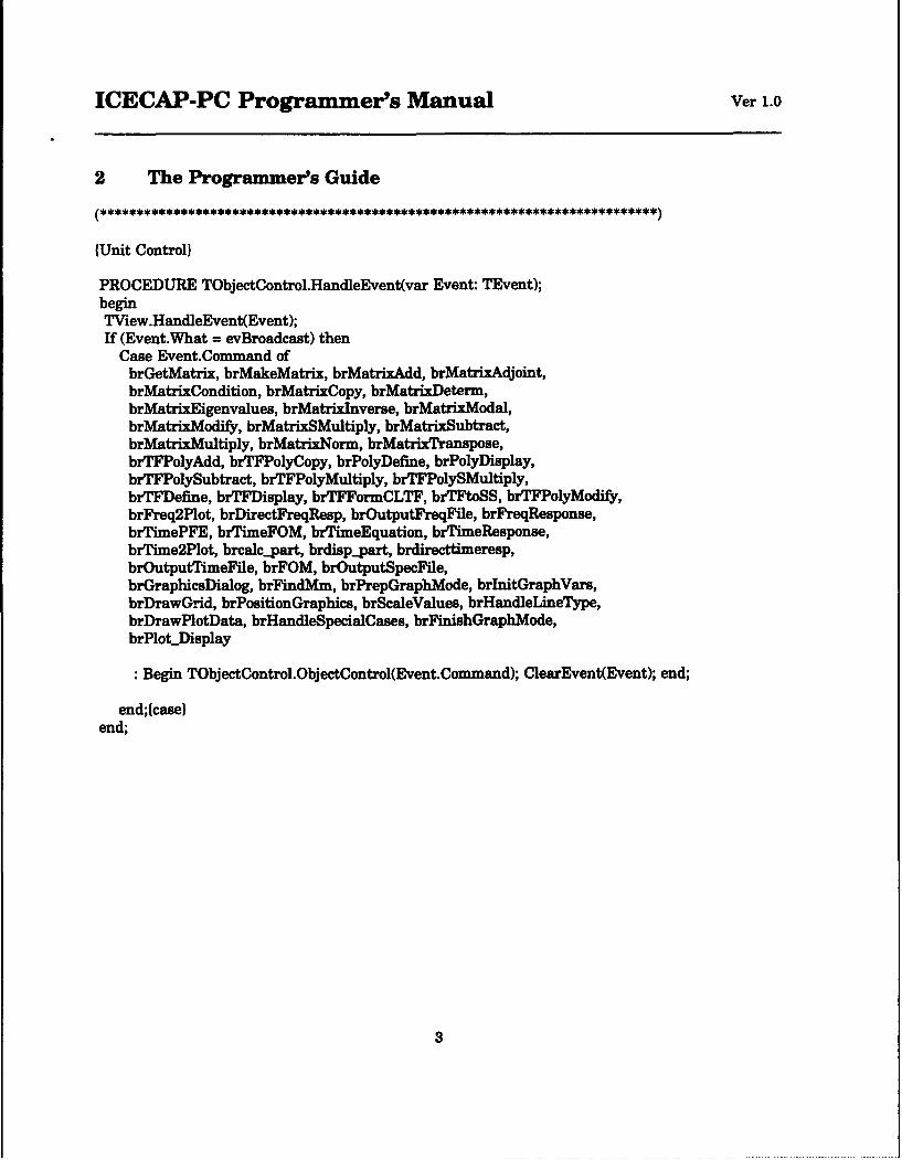
ICECAP-PC Programmer's Manual Ver 1.0
2 The Programmer's Guide
(Unit Control)
PROCEDURE TObjectControl.HandleEvent(var Event: TEvent);beginTView.HandleEvent(Event);If (Event.What = evBroadcast) then
Case Event.Command ofbrGetMatrix, brMakeMatrix, brMatrixAdd, brMatrixAdjoint,brMatrixCondition, brMatrixCopy, brMatrixDeterm,brMatrixEigenvalues, brMatrixlnverse, brMatrixModal,brMatrixModify, brMatrixSMultiply, brMatrix~ubtract,brMatzixMultiply, brMatrixNorm, brMatrixTranspose,brTFPolyAdd, brTF~olyCopy, brPolyDefine, brPolyDisplay,brTFPolySubtract, brTFPolyMultiply, brTFPolySMultiply,brTFDefine, brTFDisplay, brTFFormCLTF, brTFtoSS, brTFPolyModify,brFreq2Plot, brDirectFreqResp, brOutputFreqFile, brFreqResponse,brTimePFE, brfimeFOM, brfimeEquation, brTimeResponse,brTime2Plot, brcalc...psrt, brdisp-part, brdirecttimeresp,brOutputlimeFile, brFOM, brOutputSpecFile,brGraplucsDialog, brFindMm, brPrepGrapbMode, brlImtGraphVars,brDrawGrid, brPositionGraphics, brScaleValues, brHandleLineType,brDrawPlotData, brHandleSpecialCases, brFinishGraphMode,brPloiLDisplay
: Begin TObjectControl.ObjectControl(Event.Command); ClearEvent(Event); end;
end;(case)
end;
3
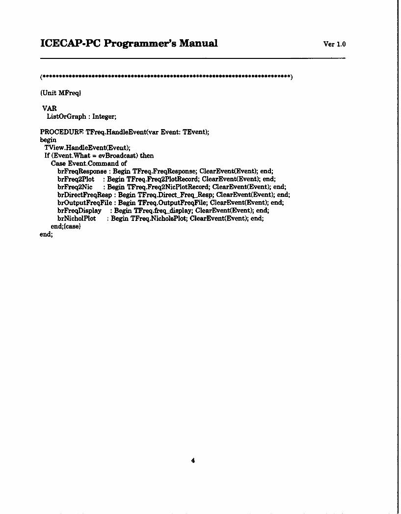
ICECAP-PC Programmer's Manual Ver 1.0
(Unit MFreqJ
VARListOrGraph :Integer;
PROCEDURE~ TFreq.HandleEvent(var Event: TEvent);begin
TWiew.HandleEvent(Event);If (Event.What = evBroadcast) then
Case Event.Command ofbrF'reqResponse : Begin TFreq.FreqResponse; ClearEvent(Event); end;brFreq2Plot :Begin TWreq.Freq2PlotRecord; ClearEvent(Event); end;brFreq2Nic :Begin TFreq.Freq2Nic~lotRecord; ClearEvent(Event); end;brDirectFreqResp :Begin TFreq.Direct Frec-Resp; ClearEvent(Event); end;brOutputFreqFile: Begin TFreq.OutputFreqFile; ClearEvent(Event); end;brF'reqDisplay : Begin TFreq.frecjdisplay; ClearEvent(Event); end;brNicholPlot :Begin TWreq.NicholsPlot; ClearEvent(Event); end;
end;{case)end;
4
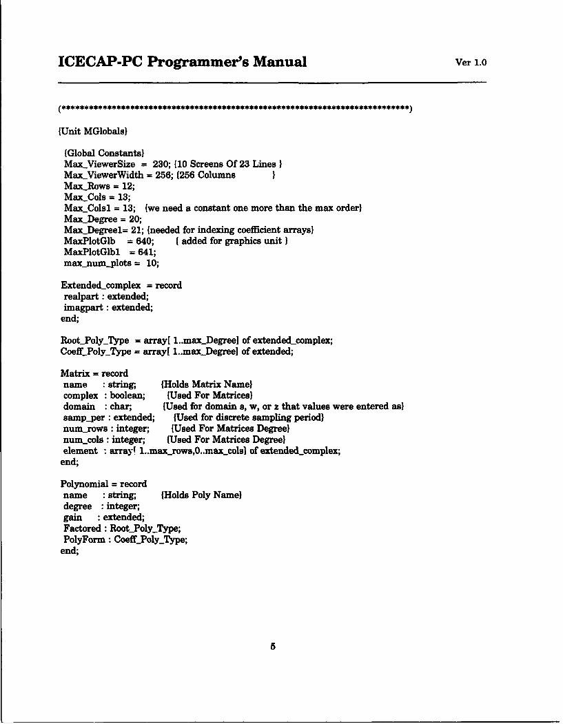
ICECAP-PC Programmer's Manual Ver 1.0
(Unit MGlobalsI
(Global Constants)MaxViewerSize = 230; 110 Screens Of 23 Lines)Max_ViewerWidth = 256; (256 ColumnsMaxRows = 12;Max_Cols = 13;MaxColsl = 13; (we need a constant one more than the max order)Max_Degree = 20;MaxDegreel= 21; (needed for indexing coefficient arrays)MaxPlotGlb = 640; (added for graphics unit IMaxPlotGlbl = 641;max_num-plots = 10;
Extended-complex = recordrealpart : extended;imagpart : extended;
end;
RootPolyType = array[ 1..maxDegreel of extended_complex;Coeff_PolyType = array[ 1..maxDegree] of extended;
Matrix = recordname string;, (Holds Matrix Name)complex boolean; (Used For Matrices)domain char; (Used for domain s, w, or z that values were entered as)samp-per : extended; {Used for discrete sampling period)numrows : integer; (Used For Matrices Degree)numcols integer; (Used For Matrices Degree)element array! 1..maxrows,0..max.cols] of extended_complex;
end;
Polynomial = recordname : string;, (Holds Poly Name)degree :integer;gain extended;Factored : RootPolyType;PolyForm - CoeffPolyType;
end;
5

ICECAP-PC Programmer's Manual Ver 1.0
TransFunc = recordname string; (Holds TF Name}domain :char; (Used for domain s, w, or z that values were entered as)samp-per : extended; (Used for discrete sampling period)num : Polynomial;den Polynomial;
end;
PolyPtr = APolynomial;TFPtr = ^TransFunc;MatPtr = AMatrix;
vectorarray = array[ 1..MaxPlotGlbl ] of extended; (7k)PlotDataType = Record
DataFileName : String;DataFile File of Extended;HorzValue,VertValue . VectorArray;Grid,LastPlot Boolean;MaxHorzAxis,MaxVertAxis,MinHorzAxis,MinVertAxis Extended;Color,DisplayCount,LogOrLinear,Nichols,NormOrDec,NumDecade,NumPlot,NumPoint,PowerOfTen Integer;Palette PaletteType;GenTitle,HorzTitle,Title,VertTitle,Mm,Wm String;
end;
6
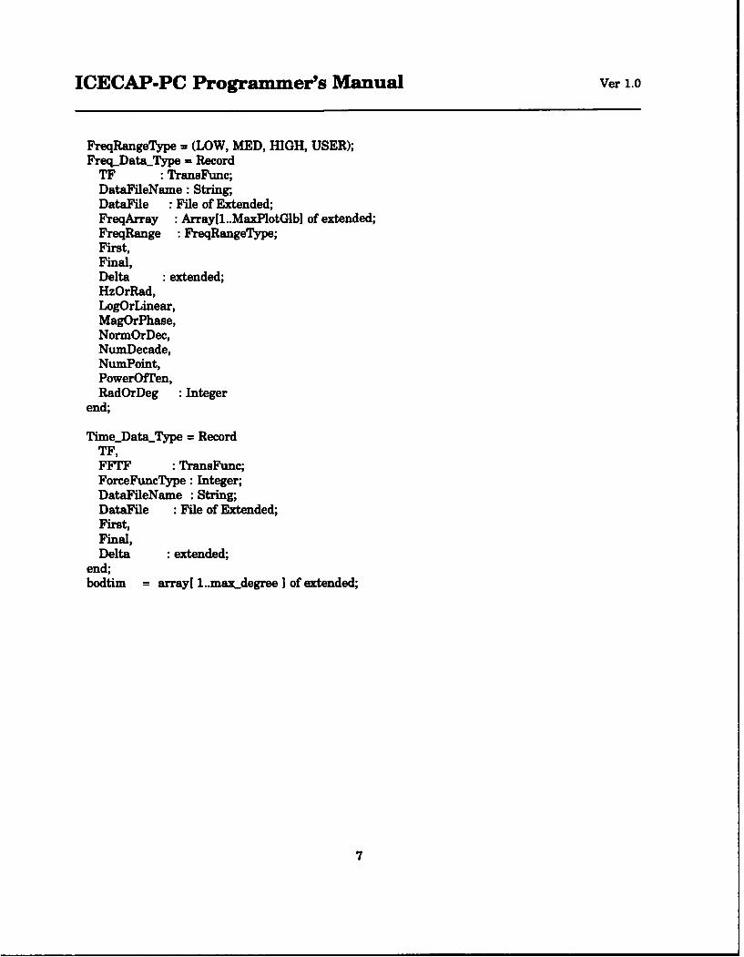
ICECAP-PC Programmrer's Manual Ver 1.0
FreqRangeType =(LOW, MED, HIGH, USER);FreqData-Type =Record
TF :TransFunc;DataFileName :String;DataFile File of Extended;FreqArray Array[1..MaxPlotGlb] of extended;FreqRange FreqRangeType;First,Final,Delta extended;HzOrRad,LogOrLinear,MagOrPhase,NormOrDec,NumDecade,NumPoint,PowerOffen,RadOrDeg :Integer
end;
Tine-Data-Type = RecordTF,FFTF TransFunc;ForceFuncType: Integer;DataFileName String;DataFile File of Extended;First,Final,Delta extended;
end;bodtim = array[l1..ma&xdegree I of extended;
7
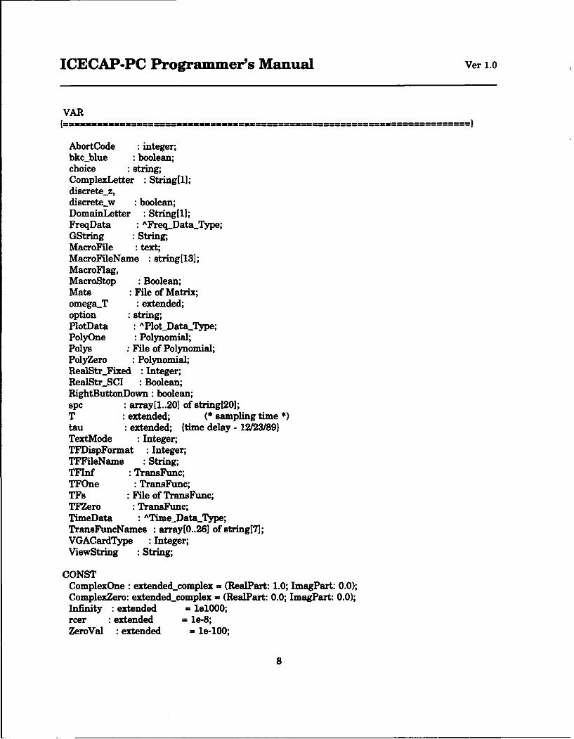
ICECAP-PC Programmer's Manual Ver 1.0
VAR
AbortCode integer;bkc-blue boolean;choice string;ComplexLetter :Stringil];discrete-z,discrete-w boolean;DomainLetter :String[ll;FreqData A~reC.Data.Type;GString String;MacroFile text;MacroFileNa~me :stringi 13];MacroFlag,MacroStop Boolean;mats File of Matrix;omegaT :extended;option string;PlotData A PlotDatajI'ype;PolyrOne Polynomial;Polys File of Polynomial;PolyZero :Polynomial;RealStrFixed Integer;RealStr_-SCI Boolean;RightButtonDown : boolean;spc arrayfl..20] of string[201;T extended; (* sampling time *tau extended; (time delay - 12/23/89)TextMode Integer;TFT~ispFormat Integer;TF~FleName String;TFInf TransFunc;TFOne :TransFunc;TFs .File of TransFunc;TFZero TransFunc;TimeData :A¶J~eDataType;TransFuncNames :array[O..261 of stringi?];VGACardTijpe :Integer;ViewString String;
CONSTComplexOne :extended-complex =(RealPart: 1.0; ImagPart: 0.0);ComplexZero: extended-complex =(RealPart: 0.0; ImagPart: 0.0);Infinity extended W eONO;rcer :extended =le-8;
ZeroVal :extended =le-100;
8
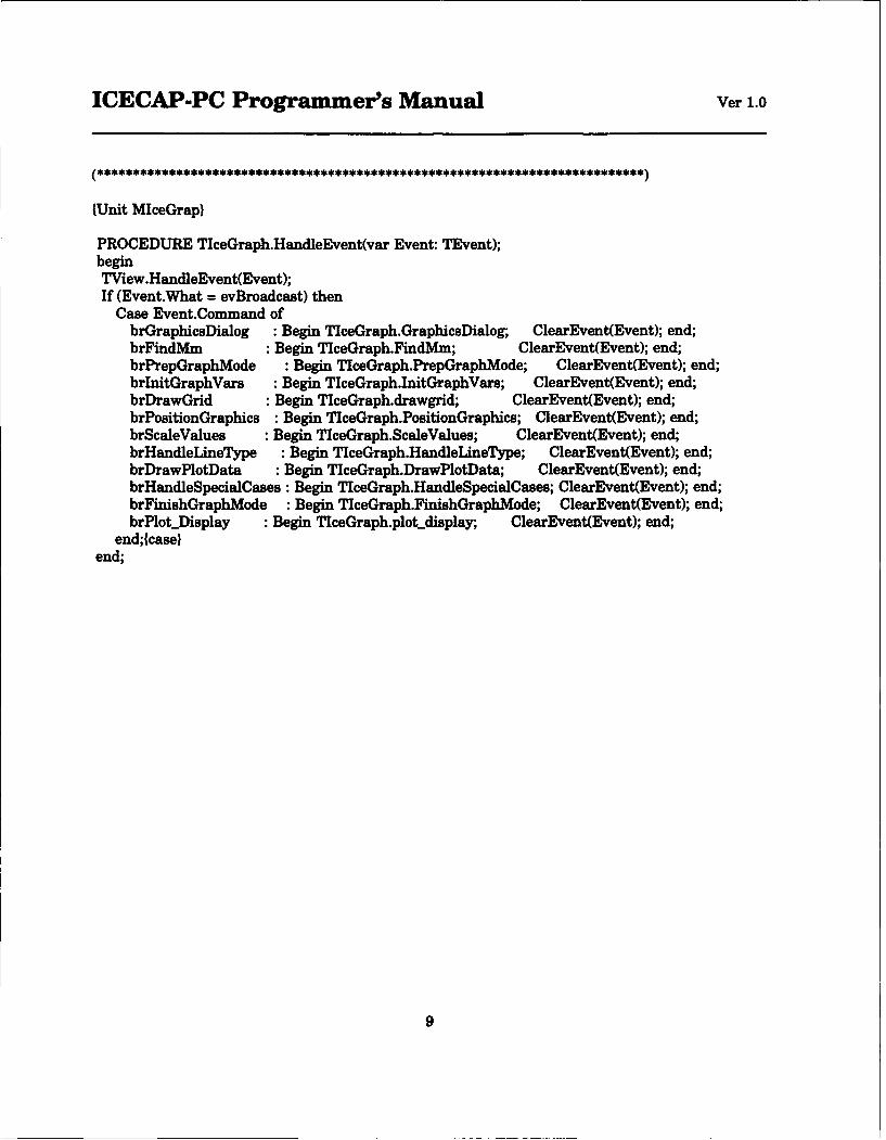
ICECAP-PC Programmer's Manual Ver 1.0
(Unit MlceGrap)
PROCEDURE TlceGraph.HandleEvent(var Event: TEvent);beginTView.HandleEvent(Event);If (Event.What = evBroadcast) then
Case Event.Command ofbrGraphicsDialog : Begin TlceGraph.GraphicoDialog; ClearEvent(Event); end;brFindMm : Begin TlceGraph.FindMm; ClearEvent(Event); end;brPrepGraphMode : Begin TlceGraph.PrepGraphMode; ClearEvent(Event); end;brlnitGraphVars :Begin TlceGraph.InitGraphVars; ClearEvent(Event); end;brDrawGrid : Begin TlceGraph.drawgrid; ClearEvent(Event); end;brPositionGraphics : Begin TlceGraph.PositionGraphics; ClearEvent(Event); end;brScaleValues : Begin TlceGraph.ScaleValues; ClearEvent(Event); end;brHandleLineType :Begin TlceGraph.HandleLineType; ClearEvent(Event); end;brDrawPlotData :Begin TlceGraph.DrawPlotData; ClearEvent(Event); end;brHandleSpecialCases : Begin TlceGraph.HandleSpecialCases; ClearEvent(Event); end;brFinishGrapbMode : Begin TlceGraph.FinishGrapbMode; ClearEvent(Event); end;brPlot-.Display :Begin TlceGraph.plot...isplay; ClearEvent(Event); end;
end;fcase)end;
9
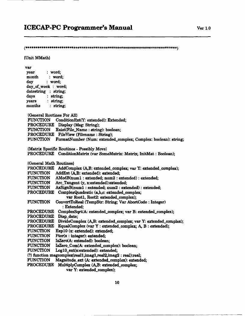
ICECAP-PC Programmer's Manual Ver 1.0
(Unit MMath)
varyear word;month word;day word;day.of_week : word;datestring : string;days : string;years : string;months string;
(General Routines For All)FUNCTION ConditionExt(Y: extended): Extended;PROCEDURE Display (Msg: String);FUNCTION Exist(FileName : string): boolean;PROCEDURE FileView (Filename : String);FUNCTION FormatNumber (Num: extendedcomplex; Complex: boolean): string;
(Matrix Specific Routines - Possibly Move)PROCEDURE ConditionMatrix (var SomeMatrix: Matrix; InitMat : Boolean);
(General Math Routines)PROCEDURE AddComplex (AB: extendedcomplex; var Y: extendedtcomplex);FUNCTION AddExt (AB: extended): extended;FUNCTION AModB(numl : extended; num2 : extended) : extended;FUNCTION Arcfangent (y, x:extended):extended;FUNCTION AxSignB(numl : extended; num2 : extended): extended;PROCEDURE ComplexQuadratic (a,b,c: extended_complex;
var Root1, Root2: extended-complex);FUNCTION ConvertToReal (TempStr: String; Var AbortCode : Integer)
: Extended;PROCEDURE ComplexSqrt(k extendedcomplex; var B: extendedcomplex);PROCEDURE Disp-date;PROCEDURE DivideComplex (AB: extended~complex; var Y: extended-complex);PROCEDURE EqualComplex (var Y : extended-complex; A, B : extended);FUNCTION Expl0 (x: extended): extended;FUNCTION Ftor(x : integer): extended;FUNCTION IsZero(A: extended): boolean;FUNCTION IsZeroCom(A: extended-complex): boolean;FUNCTION Logl0_ext(x:extended): extended;{?) function magcomplex(reallimagl,real2,imag2 : real):real;FUNCTION Magnitude-ext (A: extended-complex): extended;PROCEDURE MultiplyComplex (AB: extended-complex;
var Y: extended-complex);
10
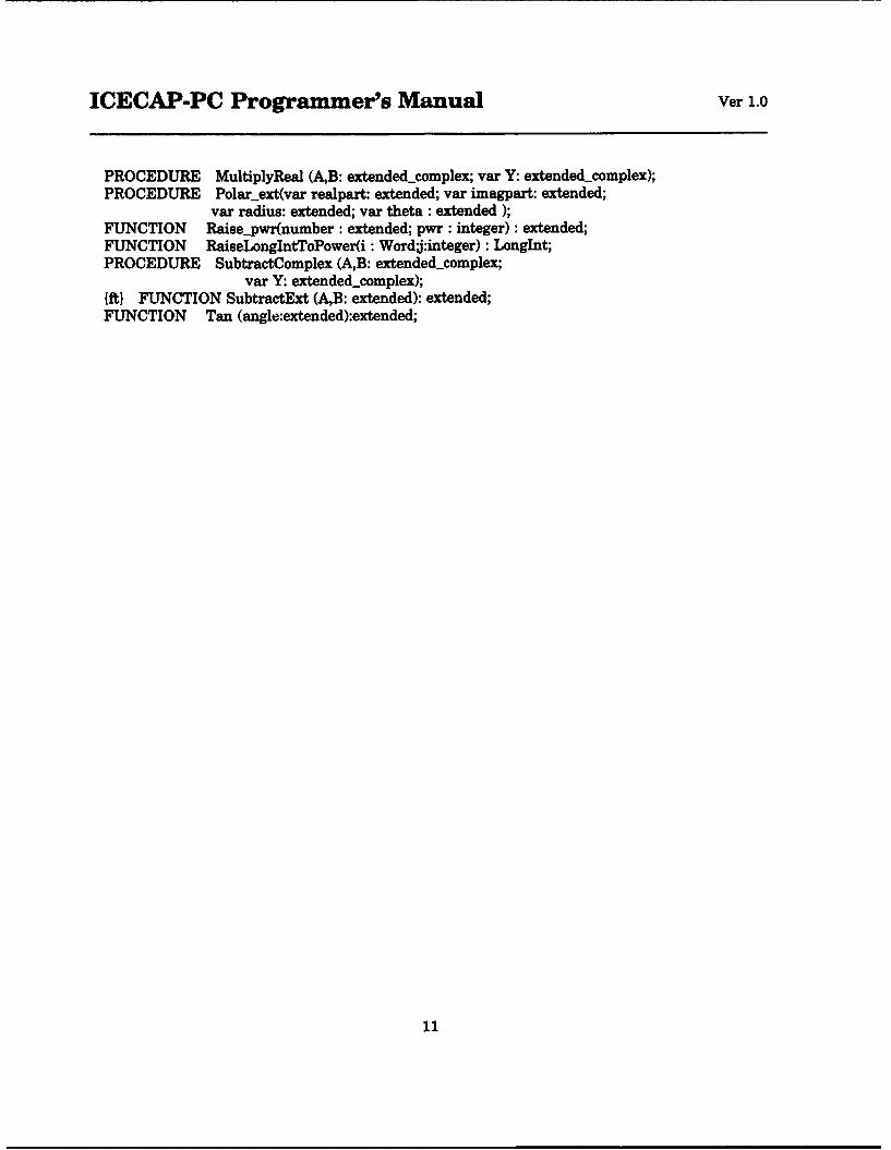
ICECAP-PC Programmer's Manual Ver 1.0
PROCEDURE MultiplyReal (AB: extendedcomplex; var Y: extended-complex);PROCEDURE Polar_ext(var realpart: extended; var imagpart: extended;
var radius: extended; var theta : extended );FUNCTION Raise-pwr(number : extended; pwr : integer): extended;FUNCTION RaiseLonglntToPower(i : Wordj:integer) : LongInt;PROCEDURE SubtractComplex (A,B: extended-complex;
var Y: extendedcomplex);Ift} FUNCTION SubtractExt (AB: extended): extended;FUNCTION Tan (angle:extended):extended;
11
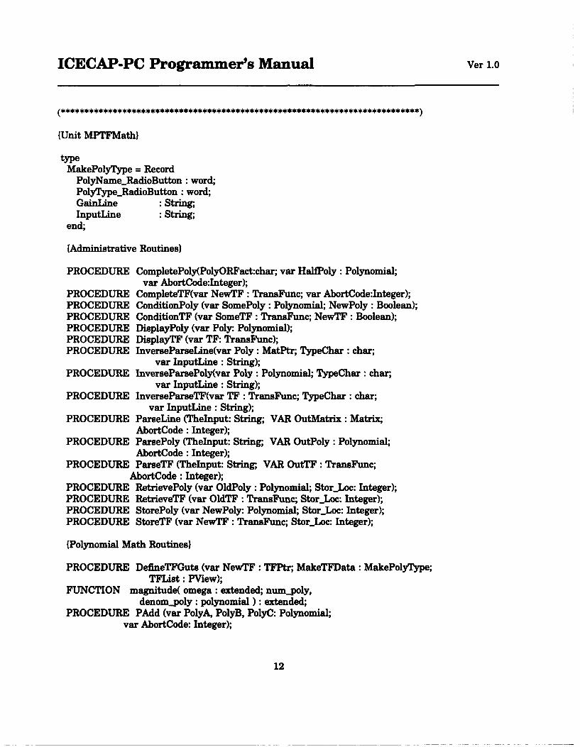
ICECAP-PC Programmer's Manual Ver 1.0
(Unit MPTFMath)
typeMakePolyType = Record
PolyNameRadioButton word;PolyTypeRadioButton : word;GainLine : String;InputLine String;
end;
(Administrative Routines)
PROCEDURE CompletePoly(PolyORFact:char; var HalfPoly Polynomial;var AbortCode:Integer);
PROCEDURE CompleteTF(var NewTF : TransFunc; var AbortCode:Integer);PROCEDURE ConditionPoly (var SomePoly: Polynomial; NewPoly: Boolean);PROCEDURE ConditionTF (var SomeTF : TransFunc; NewTF : Boolean);PROCEDURE DisplayPoly (var Poly: Polynomial);PROCEDURE DisplayTF (var TF: TransFunc);PROCEDURE InverseParseLine(var Poly: MatPtr; TypeChar : char;
var InputLine : String);PROCEDURE InverseParsePoly(var Poly : Polynomial; TypeChar : char;
var InputLine : String);PROCEDURE InverseParseTF(var TF : TransFunc; TypeChar : char;
var InputLine : String);PROCEDURE ParseLine (TheInput: String; VAR OutMatrix : Matrix;
AbortCode : Integer);PROCEDURE ParsePoly (TheInput: String-, VAR OutPoly :Polynomial;
AbortCode : Integer);PROCEDURE ParseTF (TheInput: String;, VAR OutTF : TransFunc;
AbortCode : Integer);PROCEDURE RetrievePoly (var OldPoly : Polynomial; StorLoc: Integer);PROCEDURE RetrieveTF (var OldTF : TransFunc; StorLoc: Integer);PROCEDURE StorePoly (var NewPoly: Polynomial; StorLoc: Integer);PROCEDURE StoreTF (var NewTF : TransFunc; Stor_.Loc: Integer);
(Polynomial Math Routines)
PROCEDURE DefineTFGuts (var NewTF : TFPtr; MakeTFData : MakePolyType;TFList: PView);
FUNCTION magnitude( omega: extended; num-poly,denom-.poly : polynomial ) : extended;
PROCEDURE PAdd (var PolyA, PolyB, PolyC: Polynomial;var AbortCode: Integer);
12

ICECAP-PC Programmer's Manual Ver 1.0
PROCEDURE PDivide (var N1, D1, NLSimplified, DlSimplified: Polynomial; var Abortcode : Integer);
FUNCTION phaseoangle( omega: extended; num.poly,denom-poly : polynomial ) : extended;
PROCEDURE PMult (var PolyA, PolyB, PolyC: Polynomial;var AbortCode: Integer);
PROCEDURE PScalarMult (number : extended; var PolyA,PolyB : Polynomial; var AbortCode : Integer);
PROCEDURE PSubtract (var PolyA, PolyB, PolyC: Polynomial;var AbortCode : Integer);
PROCEDURE RootCancel (var N1, D1, NSimplified, Dl_Simplified: Polynomial; var AbortCode : Integer);
PROCEDURE TFAdd(var TFA, TFB, TFC : TransFunc; var AbortCode:Integer);PROCEDURE TFDivide(var TFA, TFB, TFC : TransFunc;
var AbortCode:Integer);PROCEDURE TFMult(var TFA, TFB, TFC : TransFunc; var AbortCode:Integer);PROCEDURE TFScalarMult(ANumber : extended; var TFA, TFB : TransFunc;
var AbortCode : Integer);PROCEDURE TFSubtract(var TFA, TFB, TFC : TransFunc;
var AbortCode : Integer);
******** ********** ********** ** ****** ****** ***************** **** ***** ** *******
(Unit MRoots)
PROCEDURE Bairstow(VAR ThePoly: Polynomial; VAR b,c: extended; eps: extended);FUNCTION BrentsMethod(ThePoly: Polynomial; x.,x2,tol: extended): extended;PROCEDURE BuildFromRoots(var ReturnPoly : polynomial);PROCEDURE EvalThePoly(var ThisPoly: Polynomial; ForThisX: extended; var Ans, dp:
extended);PROCEDURE Laguer(VAR a: Root_PolyType; m: integer; VAR x: Extended_Complex);PROCEDURE LaguerreDriver(VAR ThePoly: Polynomial);FUNCTION NewtRap (var ThisPoly: Polynomial; x1 x2 xacc: extended): extended;PROCEDURE PolDiv(var u: Coeff_Polyfype; n: Integer; v: Coeff_PolyType; nv: Integer; var q,r:
Coeff_PolyType);PROCEDURE RootAccuracy (var Poly: Polynomial; var RtErrBound:extended);PROCEDURE RootFinder(var ThePoly: Polynomial);PROCEDURE SortRoots (var Poly: Polynomial);
13
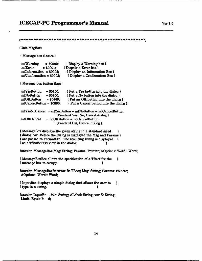
ICECAP-PC Programmer's Manual Ver 1.0
(Unit MsgBox)
( Message box classes }
mfWarning = $0000; (Display a Warning box)mfError = $0001; J Dispaly a Error box )mflnformation = $0002; ( Display an Information Box)mfConfirmation = $0003; (Display a Confirmation Box)
( Message box button flags)
mfYesButton = $0100; ( Put a Yes button into the dialog)mfNoButton = $0200; ( Put a No button into the dialog )mfOKButton = $0400; (Put an OK button into the dialog }mfCancelButton = $0800; (Put a Cancel button into the dialog)
mfYesNoCancel = mfYesButton + mfnNoButton + mfCancelButton;( Standard Yes, No, Cancel dialog)
mfOKCancel = mfOKButton + mfCancelButton;( Standard OK, Cancel dialog I
I MessageBox displays the given string in a standard sized II dialog box. Before the dialog is displayed the Msg and Params)I are passed to FormatStr. The resulting string is displayed( as a TStaticText view in the dialog.
function MessageBox(Msg: String; Params: Pointer; AOptions: Word): Word;
( MessageBoxRec allows the specification of a TRect for the( message box to occupy.
function MessageBoxRect(var R: TRect; Msg: String; Params: Pointer;AOptions: Word): Word;
I InputBox displays a simple dialog that allows the user to{ type in a string.
function InputB- Aitle: String; ALabel: String; var S: String;Limit: Byte): V A;
14
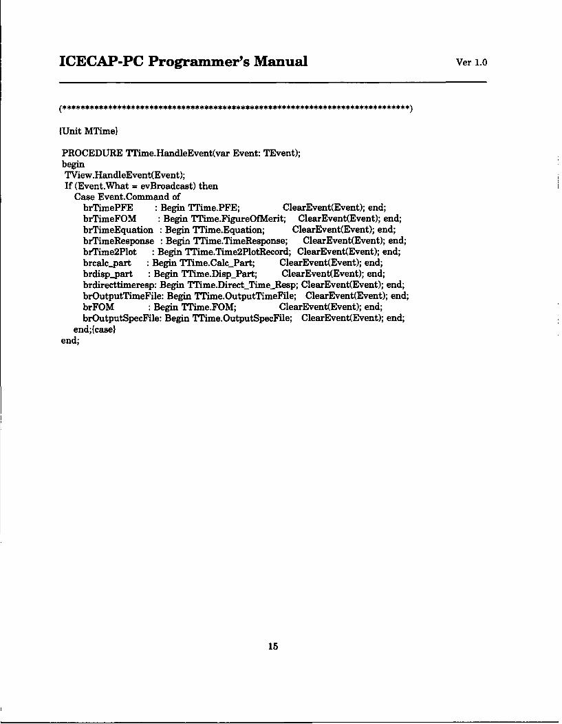
ICECAP-PC Programmer's Manual Ver 1.0
(Unit MWime)
PROCEDURE ¶I~me.HandleEvent(var Event: TEvent);beginTView.HandleEvent(Event);If (Event.What = evBroadcast) then
Case Event.Command ofbrTimePFE :Begin Tflime.PFE; ClearEvent(Event); end;brTimeFOM :Begin T7ime.FigureOfflerit; ClearEvent(Event); end;brfimeEquation :Begin T7ime.Equation; ClearEvent(Event); end;brTimeResponse :Begin TTime.TimeResponse; ClearEvent(Event); end;brTime2Plot : Begin Ti~me.Time2PotRecord; ClearEvent(Event); end;brcalc..part :Begin TMme.CalqPart; ClearEvent(Event); end;brdisp-part :Begin TWhme.Disp-Part; ClearEvent(Event); end;brdirecttimeresp: Begin TTime.DirectTiine..Resp; ClearEvent(Event); end;brOutputTimeFile: Begin TWime.OutputTimeFile; ClearEvent(Event); end;brFOM : Begin 7TIime.FOM; ClearEvent(Event); end;brOutputSpecFile: Begin 7Time.OutputSpecFile; ClearEvent(Event); end;
end;fcaselend;
15
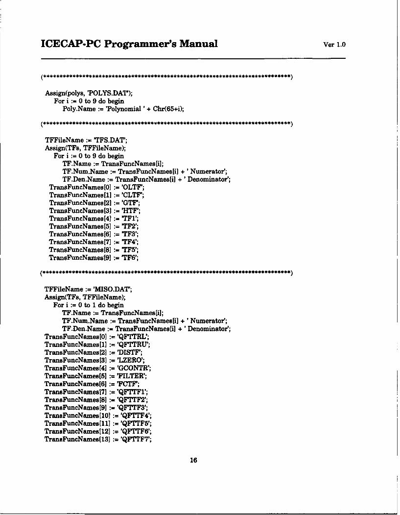
ICECAP-PC Programmer's Manual Ver 1.0
Assign(polys, 'POLYS.DAT');For i :=0 to 9 do begin
Poly.Name :='Polynomial ' + Cbr(65+i);
TFFileName:=TFS.DAT';Assign(TFs, TFFileName);
For i :=0 to 9 do beginTF.Name: TransFuncNamesfi];TF.Num.Name: TransFuncNames Ii] + 'Numerator';TF.Den.Name: TransFuncNames[iJ + 'Denominator';
TransFuncNames[0] :'OLTF";TransFuncNames [1] 'CLTF';TransFuncNames [2] 'GTF";TransFuncNames 131 'HTF';TransFuncNames [41 TF1';TransFuncNames [5] 'TF2;TransFuncNames [6] 'TF3';TransFuncNames [7] :=TF4';TransFuncNames[8] :=TF5';TransFuncNamesf91 :=TF6';
TFFileName:='MISO.DAT;Assign(TFs, TFFileName);
For i :=0 to 1 do beginTF.Name: TransFuncNames [i];TF.Num.Name: TransFuncNames[iJ + 'Numerator';TF.Den.Name: TransFuncNames[il + 'Denominator';
TransFuncNaines[0] :'QFITRL';TransFuncNames[l] :'QFTI'RU';TransFuncNames[2] 'DISTF';TransFuncNames[3] 'LZERO';TransFuncNames 141 'GCONTR';TransFuncNames[5] '=FILTER';TransFuncNames[61 := CTF";TransFuncNames 171 :'QFTTF1';TransFuncNames[81 '=QFITF2';TransFuncNames [9) := 'QFTIff3';TransFuncNames[10I :'QF1TF4';TransFuncNames[lll :'QFTI'F5';TransFuncNames[1212 :'QF-TT'F6';TransFuncNames[1313 :'QFTI'F7';
16
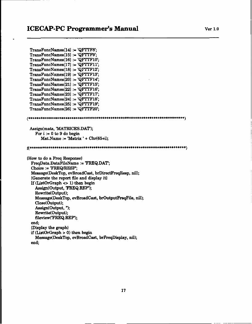
ICECAP-PC Programmer's Manual Ver 1.0
TransFuncNames[141 :'QFTTF8';TransFuncNames[15] :'QFTI'F9';TransFuncNames[1616 :'QF'JT.F10';TransFuncNames[17] :'QF'J.'I'F';TransFuncNames 1181 :'QFTITF 12';TransFuncNames[19J :'QFT.PF13';TransFuncNames[201 :'QFTI'F14';TransFuncNames[211 :'QF`ITF15';TransFuncNames[22] :'QFTI'F16';TransFuncNames[23] :'QFTI'F17';TransFuncNames[24] :'QFTTF18';TransFuncNames [25] '=QF¶1.F 19';TransFuncNames[26] :'QFTI'F20';
Assign(mats, WMATRICES.DAT");For i :=0 to 9 do begin
Mat.Name :='Matrix ' + Cbr(65+i);
(How to do a Freq ResponselFreqData.DataFileName :=FREQ.DAr;Choice: TREQIRESP';Message(DeskTop, evBroadCast, brDirectFreqResp, nil);(Generate the report ifile and display it)If (ListOrGraph <> 1) then begin
Assign(Output, 'FRQ.REP');Rewrite(Output);Message(DeskTop, evBroadCast, brOutputFreqFile, nil);CloweOutput);Assign(Output, )Rewrite(Output);ffileviewCFREQ.REP);
end;(Display the graph)if (ListOrGraph > 0) then begin
Message(DeskTop, evBroadCast, brFreqDisplay, nil);end;
17

ICECAP-PC Programmer's Manual Ver 1.0
(How to do a MultiTime Response)TimeData.DataFileName:='QFITfRUT.DATr;Choice :=I"MEIRESP';Message(DeskTop, evBroadCast, brDirectTimeResp, nil);If (List~rGraph <> 1) then begin
option :'QFTTRTY;Message(DeskTop, evBroadCast, brOutputTimeFfle, nil);
end;(Now do the Figures of Merit)Message(DeskTop, evBroadCast, brFOM, nil);If (ListOrGraph <> 1) then begin
Message(DeskTop, evBroadCast, brOutputSpecFfle, nil);Close(Output);Assign(Output, )
Rewrite(Output);fileview(TIMESPEC.REP);
end;if ListOrGraph > 0 then begin
PlotData.NumPlot: 2;TimeData.DataFileName:='QFIT1RUT.DAr';PlotData.DisplayCount: 1;Message(DeskTop, evBroadCast, brimie2Pot, nil);PlotData.LastPlot: FALSE;Message(DeskTop, evBroadCast, brplot-.display, nil);TimeData.DataFileName:='QFTTRLT.DAr;PlotData.DisplayCount: 2;Message(DeskTop, evBroadCast, brfime2Plot, nil);PlotData.LastPlot :=TRUE;Message(DeskTop, evBroadCast, brplotýdisplay, nil);
eud;
18

Appendix E QFT Toolbox User's Manual
ICECAP- PCVersion 10.0 - MS-DOS
Interactive Control Engineering Computer Analysis Packagefor the Personal Computer
QFT TOOLBOXQuantitative Feedback Theory (QFT)
User's Manual v 2.0
Professor Gary B. LamontDepartment of Electrical and Computer Engineering
School of EngineeringAir Force Institute of Technology
Wright-Patterson AFBDayton, Ohio 45433-6583
cooperative copyrighted 1992
PREFACE
WELCOME to the QFT Toolbox of ICECAP-PC. This Toolbox includes both multiple-input multiple-output (MIMO) and multiple-input single output (MISO) models in both continuous and discretedomains. ICECAP-PC is an ongoing development of a public domain computer-aided design (CAD)package for students, faculty and practitioners of control engineering and digital signal processingwith special emphasis on education. Source code and executable files are available. If you areinterested in adding additional code or have suggestions for improvement please contact:
Professor Gary B. LamontDepartment of Electrical and Computer Engineering
School of EngineeringAir Force Institute of Technology
Wright-Patterson AFB OH 45433-6583(513) 255-3450
(ARPANET [email protected])
cooperative copyright (C) 1985, 1986, 1987, 1988, 1989, 1990,1991,1992 Gary B. Lamont, Susan K.Mashiko, Gary C. Tarczynski, D. Gelopulos, Paul A. Moore, Wayne E. Bell, Vincent M. Parisi, FredTrevino, Mark W. Schiller, Ken A. Crosby
This public domain QFT-CAD package is intended for the main purpose of education and thus theexecutable code can be distributed freely. Any use of the package in support of written publicationsshould be indicated as a reference. Changes to the public domain source code that improve and extendits capabilities are appreciated, however, all suggested changes should be communicated to the authorsfor updating and dissemination of the next official version.
Permission to use, copy and distribute this software for educational purposes without fee is herebygranted provided that the copyright notice and this permission notice appear on all copies. Permissionto modify the software is granted, but not the right to distribute the modified code. All modificationsare to be distributed as changes to released versions by AFIT.
ICECAP-PC is written in Borland'st Turbo PASCAL 6.0 and TurboVision, both of which are registeredtrademarks and copyrighted by Borland International, Inc. 1800 Green Hills Road, P.O. Box 660001,Scotts Valley, CA 95067-0001. The .BGI files distributed with our package are released to publicaccess by Borland.
All references to MS-DOS in this document refer to Microsoft-DOS which is a registered trademarkand copyrighted by MicroSoftt Corporation.
QFT Notation as used in ICECAP-PC is consistent with [Houpis, 1992c].
SYSTEM REQUIREMENTS
ICECAP-PC is designed to work on MS-DOSt 80286/80386/80486 computers with a minimum of 640KB of RAM and 5MB of hard disk space. ICECAP-PC supports all graphics terminals includingHercules,, EGA and VGA. Operation is greatly enhanced with expanded memory and a math co-processor. Installation of ICECAP-PC and its QFT Toolbox is done automatically with a providedinstall procedure (see ICECAP-PC manual).
Edited By: Gary B. Lamont, Wayne E. Bell, and Fred Trevino; 1992
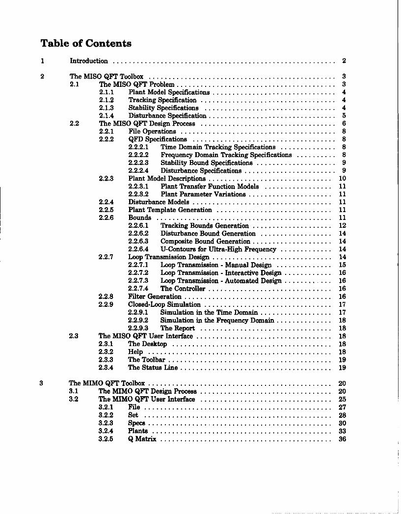
Table of Contents
Introduction ........................................................ 2
2 The MISO QFT Toolbox ............................................... 32.1 The MISO QFT Problem ........................................ 3
2.1.1 Plant Model Specifications ............................... 42.1.2 Tracking Specification .................................. 42.1.3 Stability Specifications ................................. 42.1.4 Disturbance Specification ................................ 5
2.2 The MISO QFT Design Process .................................. 62.2.1 File Operations ....................................... 82.2.2 QFD Specifications .................................... 8
2.2.2.1 Time Domain Tracking Specifications .............. 82.2.2.2 Frequency Domain Tracking Specifications .......... 82.2.2.3 Stability Bound Specifications .................... 92.2.2.4 Disturbance Specifications ....................... 9
2.2.3 Plant Model Descriptions ............................... 102.2.3.1 Plant Transfer Function Models ................. 112.2.3.2 Plant Parameter Variations ..................... 11
2.2.4 Disturbance Models ................................... 112.2.5 Plant Template Generation ............................. 112.2.6 Bounds.............................................11
2.2.6.1 Tracking Bounds Generation .................... 122.2.6.2 Disturbance Bound Generation .................. 142.2.6.3 Composite Bound Generation .................... 142.2.6.4 U-Contours for Ultra-High Frequency ............. 14
2.2.7 Loop Transmission Design .............................. 142.2.7.1 Loop Transmission - Manual Design .............. 152.2.7.2 Loop Transmission - Interactive Design ............ 162.2.7.3 Loop Transmission - Automated Design ............. 162.2.7.4 The Controller ............................... 16
2.2.8 Filter Generation ..................................... 162.2.9 Closed-Loop Simulation ................................ 17
2.2.9.1 Simulation in the Time Domain .................. 172.2.9.2 Simulation in the Frequency Domain .............. 182.2.9.3 The Report ................................. 18
2.3 The MISO QFT User Interface .................................. 182.3.1 The Desktop ........................................ 182.3.2 H elp .............................................. 182.3.3 The Toolbar ......................................... 192.3.4 The Status Line ...................................... 19
3 The MIMO QFT Toolbox .............................................. 203.1 The MIMO QFT Design Process ................................. 203.2 The MIMO QFT User Interface ................................. 25
3.2.1 File ............................................... 273.2.2 Set ............................................... 283.2.3 Specs .............................................. 303.2.4 Plants ............................................. 333.2.5 Q M atrix ........................................... 36

4 Design Examples ................................................... 384.1 MIMO QFT Design Example ................................... 384.2 MISO QFT Design Example .................................... 43
QFT Toolbox User's Manual Ver 2.0
1 Introduction
One objective of ICECAP-PC, as well as its associated toolboxes, is to provide a 4thgeneration language (4GL) interface for control engineering students and practitioners. This 4GLinterface allows ICECAP-PC's functions and operations to be used as an end product within itswindow-based desktop environment, or as an object-oriented macro language for new user productscalled toolbox extensions. The window-based desktop interface provides pull-down menus, speed-buttons, mouse support, hot keys and on-line, context-sensitive HELP, all of which combines tomake ICECAP-PC very user friendly as well as effective!
ICECAP-PC and the QFT toolbox was developed using Borland's, object-orientedTurboVision language (a 4GL) under Turbo Pascal. Top pull-down menu selections produce dialogboxes from which the user defines an operation. The pull-down menu is always accessibleproviding a truly event-driven and nimble interface. System parameters are quickly modified withrecall of past inputs providing efficient interactive analysis and synthesis of the controller. TheQFT toolbox is invoked from the ICECAP-PC main menu by selecting either the Toolbox - MIMOQFT or Toolbox - MISO QFT menu options.
The overviews of the MIMO and MISO model QFT design techniques are presented in thefollowing chapters. For supporting theoretical studies please consult references. Note that ( isused in place of jo simply to keep equations less cluttered. A complete design example is given atthe end of the manual.
2
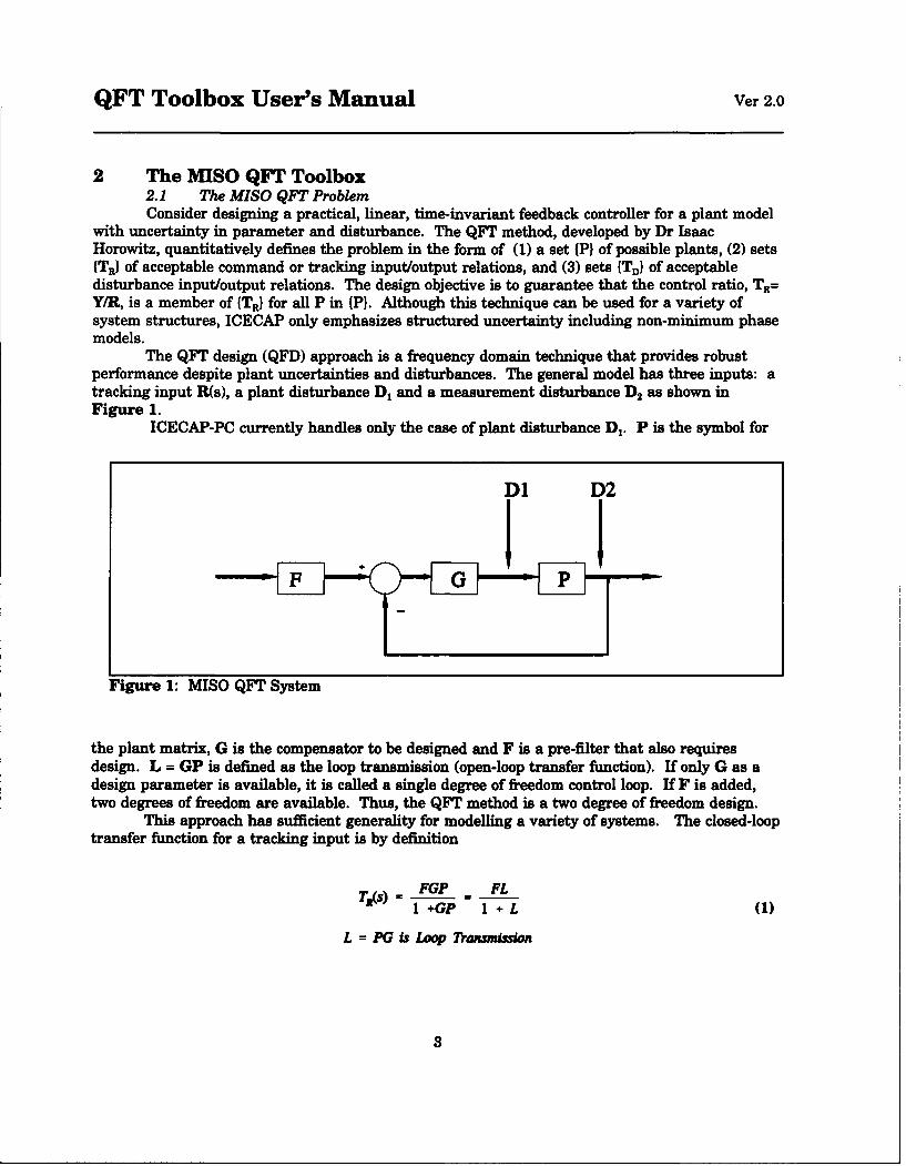
QFT Toolbox User's Manual Ver 2.0
2 The MISO QFT Toolbox2.1 The MISO QFT ProblemConsider designing a practical, linear, time-invariant feedback controller for a plant model
with uncertainty in parameter and disturbance. The QFT method, developed by Dr IsaacHorowitz, quantitatively defines the problem in the form of (1) a set {P} of possible plants, (2) sets{TRI of acceptable command or tracking input/output relations, and (3) sets {TD} of acceptabledisturbance input/output relations. The design objective is to guarantee that the control ratio, TR=
Y/R, is a member of (TRI for all P in (P). Although this technique can be used for a variety ofsystem structures, ICECAP only emphasizes structured uncertainty including non-minimum phasemodels.
The QFT design (QFD) approach is a frequency domain technique that provides robustperformance despite plant uncertainties and disturbances. The general model has three inputs: atracking input R(s), a plant disturbance D, and a measurement disturbance D2 as shown inFigure 1.
ICECAP-PC currently handles only the case of plant disturbance D,. P is the symbol for
D1 D2
Figure 1: MISO QFT System
the plant matrix, G is the compensator to be designed and F is a pre-filter that also requiresdesign. L = GP is defined as the loop transmission (open-loop transfer function). If only G as adesign parameter is available, it is called a single degree of freedom control loop. If F is added,two degrees of freedom are available. Thus, the QFT method is a two degree of freedom design.
This approach has sufficient generality for modelling a variety of systems. The closed-looptransfer function for a tracking input is by definition
TRW = FGP FLI GP 1+L (+)
L = PG is Loop Tr7waission
3
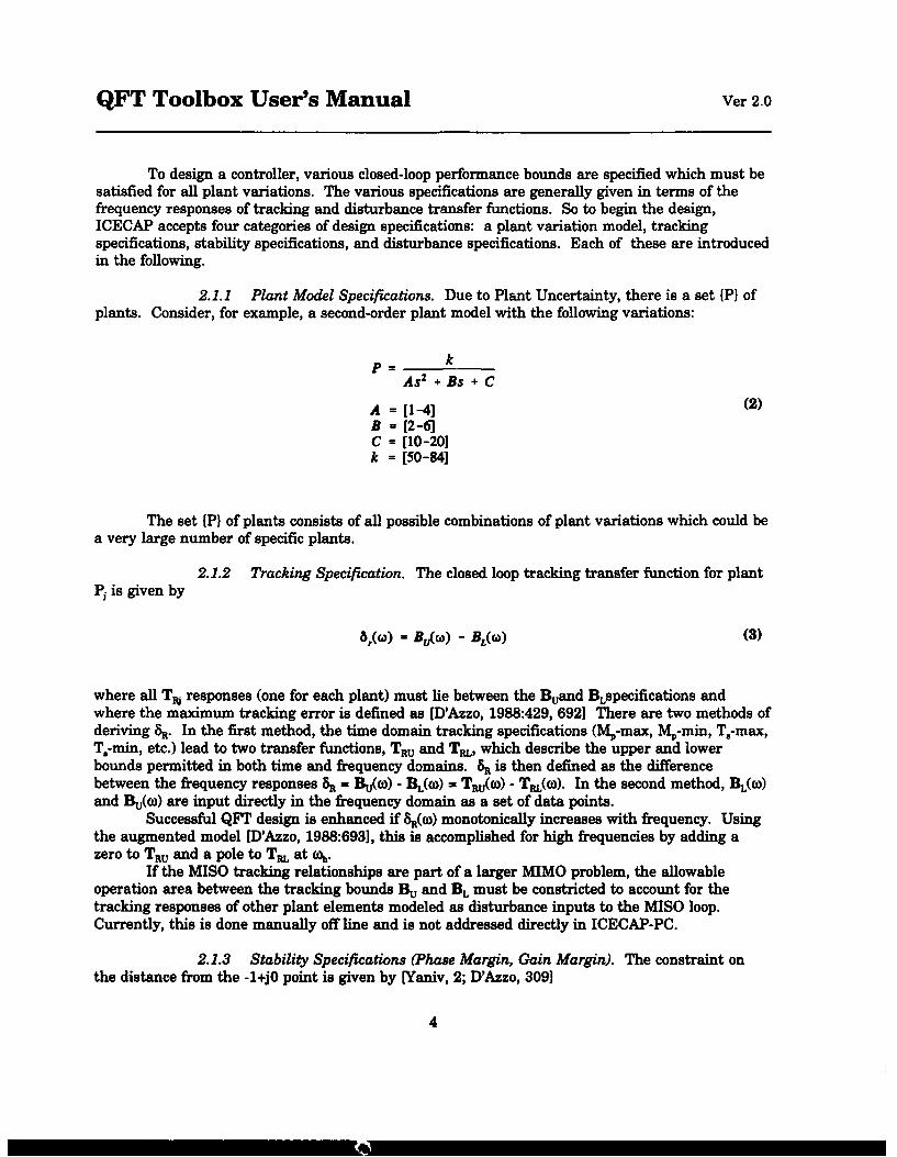
QFT Toolbox User's Manual Ver 2.0
To design a controller, various closed-loop performance bounds are specified which must besatisfied for all plant variations. The various specifications are generally given in terms of thefrequency responses of tracking and disturbance transfer functions. So to begin the design,ICECAP accepts four categories of design specifications: a plant variation model, trackingspecifications, stability specifications, and disturbance specifications. Each of these are introducedin the following.
2.1.1 Plant Model Specifications. Due to Plant Uncertainty, there is a set (P} ofplants. Consider, for example, a second-order plant model with the following variations:
k
As 2 + Bs + C
A [1-4] (2)B = [2-6]C - [10-201k = [50-84]
The set (P) of plants consists of all possible combinations of plant variations which could bea very large number of specific plants.
2.1.2 Tracking Specification. The closed loop tracking transfer function for plantPj is given by
8, = B0 ) - BL()(3)
where all T, responses (one for each plant) must lie between the Buand BLspecifications andwhere the maximum tracking error is defined as [D'Azzo, 1988:429, 692] There are two methods ofderiving 8R. In the first method, the time domain tracking specifications (Mp-max, Mp-min, T,-max,T.-min, etc.) lead to two transfer functions, TRu and TRL, which describe the upper and lowerbounds permitted in both time and frequency domains. 8R is then defined as the differencebetween the frequency responses 8R = Bj(o) - BL(w) = TRu(w) - TL(Q). In the second method, BL(0)and Bu(w) are input directly in the frequency domain as a set of data points.
Successful QFT design is enhanced if SR(w) monotonically increases with frequency. Usingthe augmented model [D'Azzo, 1988:693], this is accomplished for high frequencies by adding azero to TRu and a pole to TRL at wh.
If the MISO tracking relationships are part of a larger MIMO problem, the allowableoperation area between the tracking bounds Bu and BL must be constricted to account for thetracking responses of other plant elements modeled as disturbance inputs to the MISO loop.Currently, this is done manually off line and is not addressed directly in ICECAP-PC.
2.1.3 Stability Specifications (Phase Margin, Gain Margin). The constraint onthe distance from the -1+jO point is given by [Yaniv, 2; D'Azzo, 3091
4
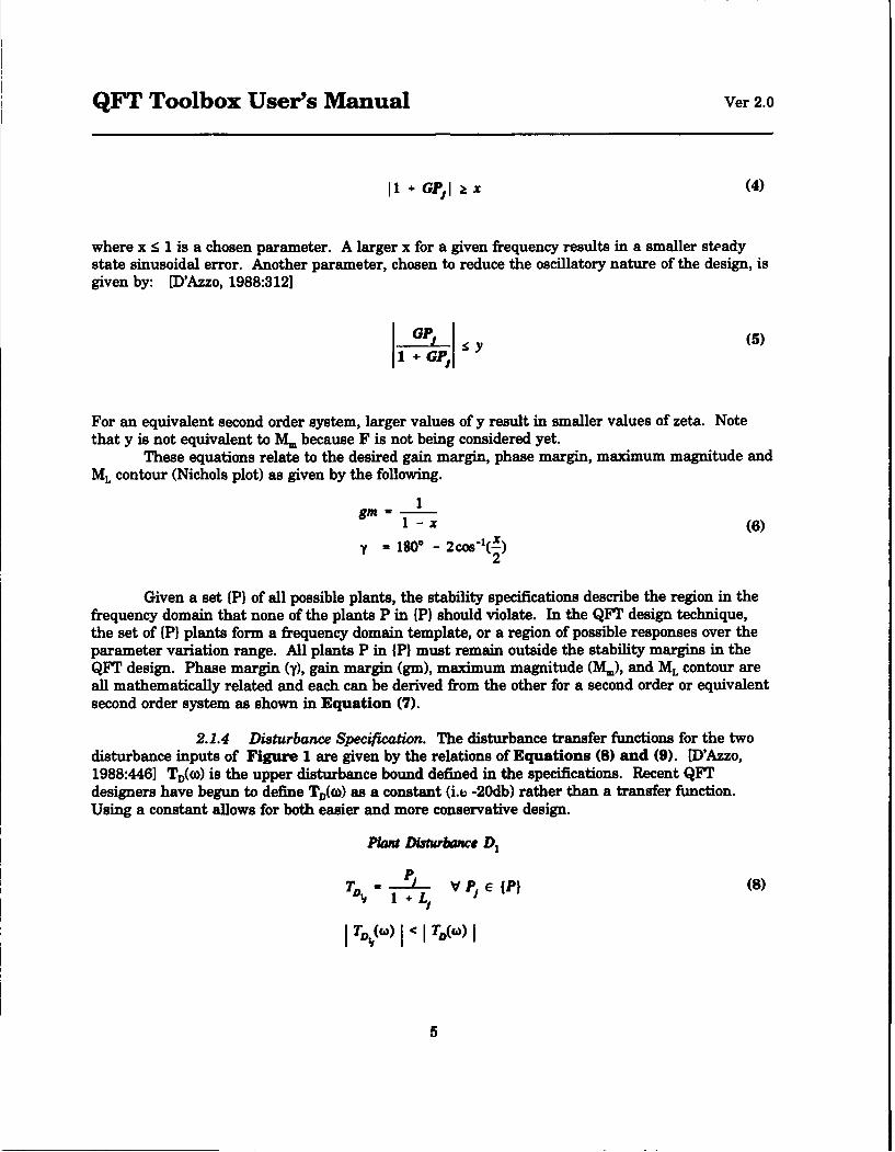
QFT Toolbox User's Manual Ver 2.0
I1 + GPJI I x (4)
where x < 1 is a chosen parameter. A larger x for a given frequency results in a smaller steadystate sinusoidal error. Another parameter, chosen to reduce the oscillatory nature of the design, isgiven by: [D'Azzo, 1988:312]
1GPj Y (5)
1+GP,
For an equivalent second order system, larger values of y result in smaller values of zeta. Notethat y is not equivalent to M. because F is not being considered yet.
These equations relate to the desired gain margin, phase margin, maximum magnitude andML contour (Nichols plot) as given by the following.
11m - X (6)
y = 180* - 2cos-1(2)2
Given a set (P) of all possible plants, the stability specifications describe the region in thefrequency domain that none of the plants P in {P) should violate. In the QFT design technique,the set of (P) plants form a frequency domain template, or a region of possible responses over theparameter variation range. All plants P in (P) must remain outside the stability margins in theQFT design. Phase margin (y), gain margin (gin), maximum magnitude (M,1), and ML contour areall mathematically related and each can be derived from the other for a second order or equivalentsecond order system as shown in Equation (7).
2.1.4 Disturbance Specification. The disturbance transfer functions for the twodisturbance inputs of Figure 1 are given by the relations of Equations (8) and (9). [D'Azzo,1988:446] TD(w) is the upper disturbance bound defined in the specifications. Recent QFTdesigners have begun to define TD(ow) as a constant (i.e -20db) rather than a transfer function.Using a constant allows for both easier and more conservative design.
Plat fiturbance DI
5
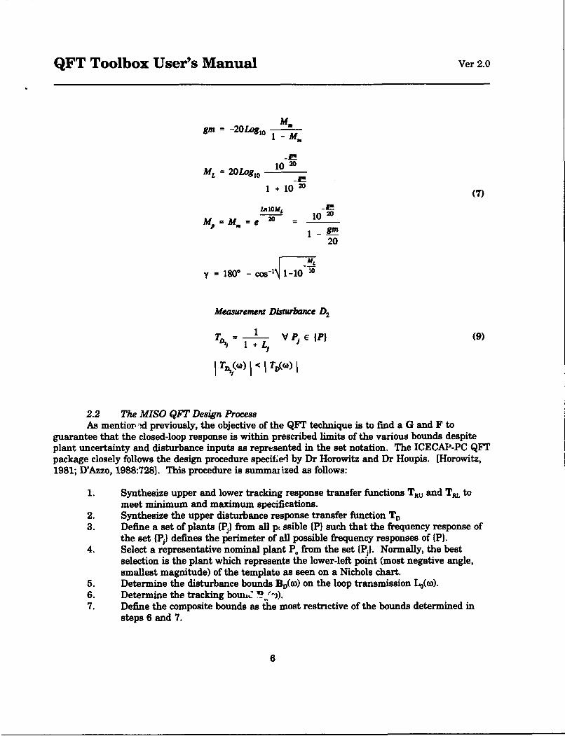
QFT Toolbox User's Manual Ver 2.0
M3gm = -20Log 1o 1 - M.
10 20
ML = 2OLog1o 0 2
1+1020 (7)
MP = mMN e 20 10 2
20
y = 180I - cos- 1-10"10
Measurement Disturbance D2
1 11 'E}(PI (9)TD + (L,
2.2 The MISO QFT Design ProcessAs mentior id previously, the objective of the QFT technique is to find a G and F to
guarantee that the closed-loop response is within prescribed limits of the various bounds despiteplant uncertainty and disturbance inputs as represented in the set notation. The ICECAP-PC QFTpackage closely follows the design procedure specified by Dr Horowitz and Dr Houpis. [Horowitz,1981; D'Azzo, 1988:728]. This procedure is summai ized as follows:
1. Synthesize upper and lower tracking response transfer functions Tsv and T. tomeet minimum and maximum specifications.
2. Synthesize the upper disturbance response transfer function TD
3. Define a set of plants {P,) from all p• ssible JP) surl that the frequency response ofthe set {P,) defines the perimeter of all possible frequency responses of (P).
4. Select a representative nominal plant P. from the set (PF). Normally, the bestselection is the plant which represents the lower-left point (most negative angle,smallest magnitude) of the template as seen on a Nichols chart.
5. Determine the disturbance bounds B0 (w) on the loop transmission L0(w).6. Determine the tracking bouu% ' .)).7. Define the composite bounds as the most restrictive of the bounds determined in
steps 6 and 7.
6
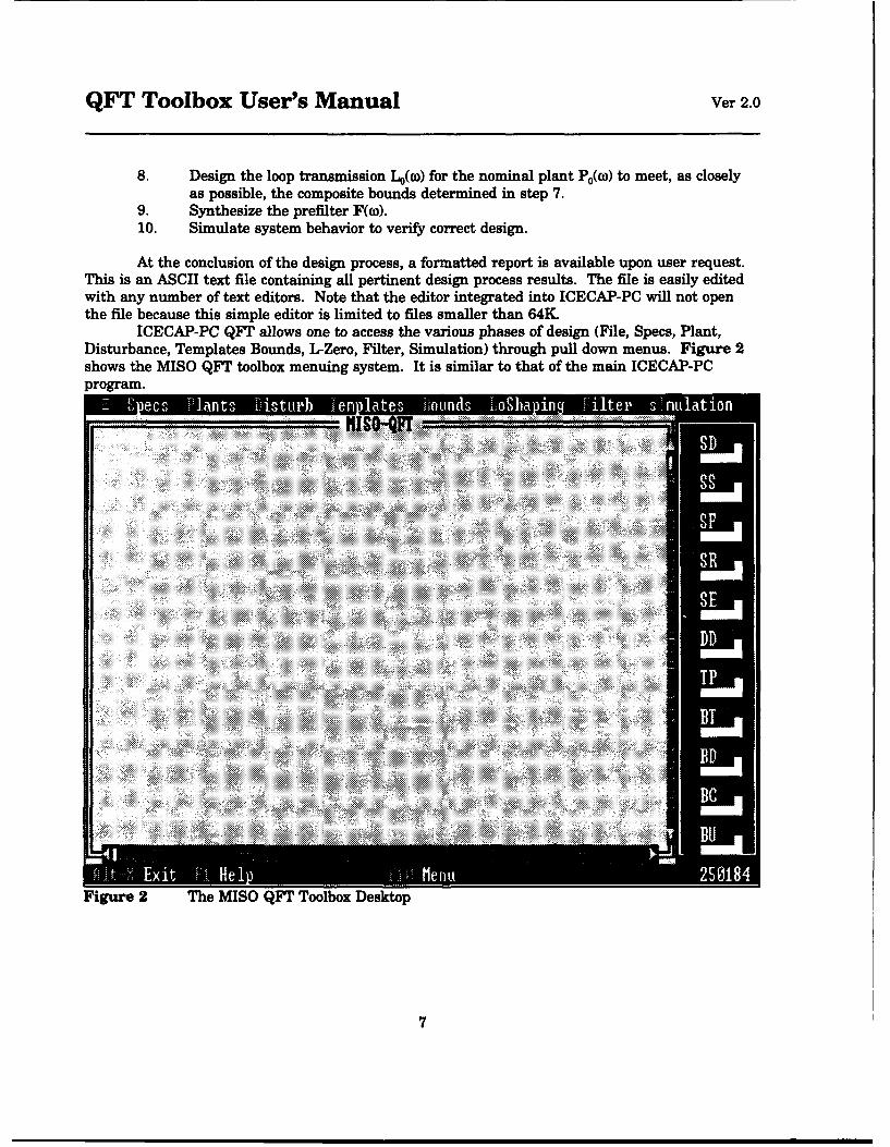
QFT Toolbox User's Manual Ver 2.0
8. Design the loop transmission Lo(o)) for the nominal plant Po(co) to meet, as closelyas possible, the composite bounds determined in step 7.
9. Synthesize the prefilter F(wo).10. Simulate system behavior to verify correct design.
At the conclusion of the design process, a formatted report is available upon user request.This is an ASCII text file containing all pertinent design process results. The file is easily editedwith any number of text editors. Note that the editor integrated into ICECAP-PC will not openthe fie because this simple editor is limited to files smaller than 64K.
ICECAP-PC QFT allows one to access the various phases of design (File, Specs, Plant,Disturbance, Templates Bounds, L-Zero, Filter, Simulation) through pull down menus. Figure 2shows the MISO QFT toolbox menuing system. It is similar to that of the main ICECAP-PCprogram.
F~ ii}!i iii ~i!'ii.............
Figure 2 The MISO QFT Toolbox Desktop
7
QFT Toolbox User's Manual Ver 2.0
The various menu items, corresponding to the high-level design steps, are initiated by using thearrow keys, mouse or control keys. For example, the introductory menu can be accessed bypressing the first letter of the desired menu selection. For example, the SPECS menu is pulleddown by S. F1 or the right mouse button displays a window with help information at the selectedlevel. Although a detailed step-by-step example could be provided, the use of the keys or mouse isself-evident. The QFT MISO example in Chapter 3 details each step of the design process asimplemented in the ICECAP-PC QFT Toolbox.
Note that during the design process, it is helpful to develop a commented log file of theunfolding design. ICECAP-PC provides this capability allowing the user to open a text log file andenter comments at any point of the design. This would be separate from the REPORT optionfound at the end of the design process.
2.2.1 File Operations. ICECAP-PC data files are generated and stored in binaryformat allowing rapid access to large amounts of data. On the other hand, all output files such astime and frequency response data, etc. are stored in ASCII form to allow easy interface to othergraphics programs. Additionally, ICECAP-PC will soon be able to read ASCII files generated fromother popular engineering programs. Such files will be checked for proper structure before theimport process begins. ICECAP-PC sessions can be saved and recalled by user defined names thusreturning the engineer to the place he left off during an interrupted design process. At the end ofthe design process, a printed report of the file contents presents the complete design record. Alsoof importance is the ability of the MISO QFT toolbox to read the separate MISO loop files createdby the MIMO toolbox. These files are opened as sessions within the MISO toolbox.
2.2.2 QFD Specifications. Three operational domains are available consisting ofthe continuous and discrete domains (s, z and w). Specifications in each case are defined in eitherthe time domain or frequency domain.
A priori synthesized tracking specifications can either be input as s-plane transferfunctions or frequency domain data. For transfer function input, the upper tracking functionbound (TRu) and the lower tracking function bound (TEL) are interactively synthesized or manuallyentered using the standard ICECAP-PC transfer function input. Transfer functions, in general,are entered in one of two forms: factored (gain, zeros and poles) or polynomial (gain andcoefficients). The time domain (TRu, TeL) or frequency domain specifications (8R(o)) can bepresented in a table or in graphical form as requested. The frequency domain data can be directlyentered as magnitude limits (max and min) vs. frequency.
Selection from the SPEC pull-down menu, Figure 3, produces a palette of options, each ofwhich result in a dialog box that defines specific actions. The options include system domain (s, z,or w), time-domain or frequency domain tracking and disturbance specification input.
2.2.2.1 Time Domain Tracking Specifications. Enter TRu(s) and TeL(s)bounds for step response tracking operations. Usually these bounds are defined in terms oftransfer functions that are synthesized from time domain specifications such as rise time, settlingtime, overshoot (the conventional figures of merit). Alternately, you may synthesize the boundsinteractively with the QFT toolboxes.
2.2.2.2 Frequency Domain Tracking Specifications. Enter TRu(co) and T.(w)bounds for the frequency range of interest. These usually are generated in transfer function. 8R(o))is the difference between Tsu(o)) and TL(W). It is desirable that TRu and TeL be synthesized suchthat 8R increases with frequency after TRu crosses the 0 dB line. An increasing 6R permits aneffective high frequency design technique. 8R can also be found from a given set of lower, BL(a)
8
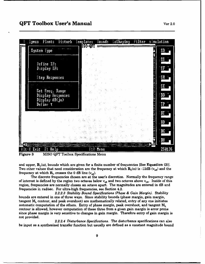
QFT Toolbox User's Manual Ver 2.0
-I
Figure 3 MISO QFT Toolbox Specifications Menu
and upper, Bu(co), bounds which are given for a finite number of frequencies [See Equation (3)].Two other values that need consideration are the frequency at which Bu(co) is -12dB (VhR) and thefrequency at which BU crosses the 0 dB line (V.R).
The discrete frequencies chosen are at the user's discretion. Normally the frequency rangeof interest is defined by the region two octaves below vR and two octaves above vhR. Inside of thisregion, frequencies are normally chosen an octave apart. The magnitudes are entered in dB andfrequencies in rad/sec. For ultra-high frequencies, see Section 4.2.
2.2.2.3 Stability Bound Specifications (Phase & Gain Margin). Stabilitybounds are entered in one of three ways. Since stability bounds (phase margin, gain margin,tangent ML contour, and peak overshoot) are mathematically related, entry of any one initiatesautomatic computation of the others. Entry of phase margin, peak overshoot, and tangent MLcontour is allowed, however computation of these three from a given gain margin is error pronesince phase margin is very sensitive to changes in gain margin. Therefore entry of gain margin isnot provided.
2.2.2.4 Disturbance Specifications. The disturbance specifications can alsobe input as a synthesized transfer function but usually are defined as a constant magnitude bound
9
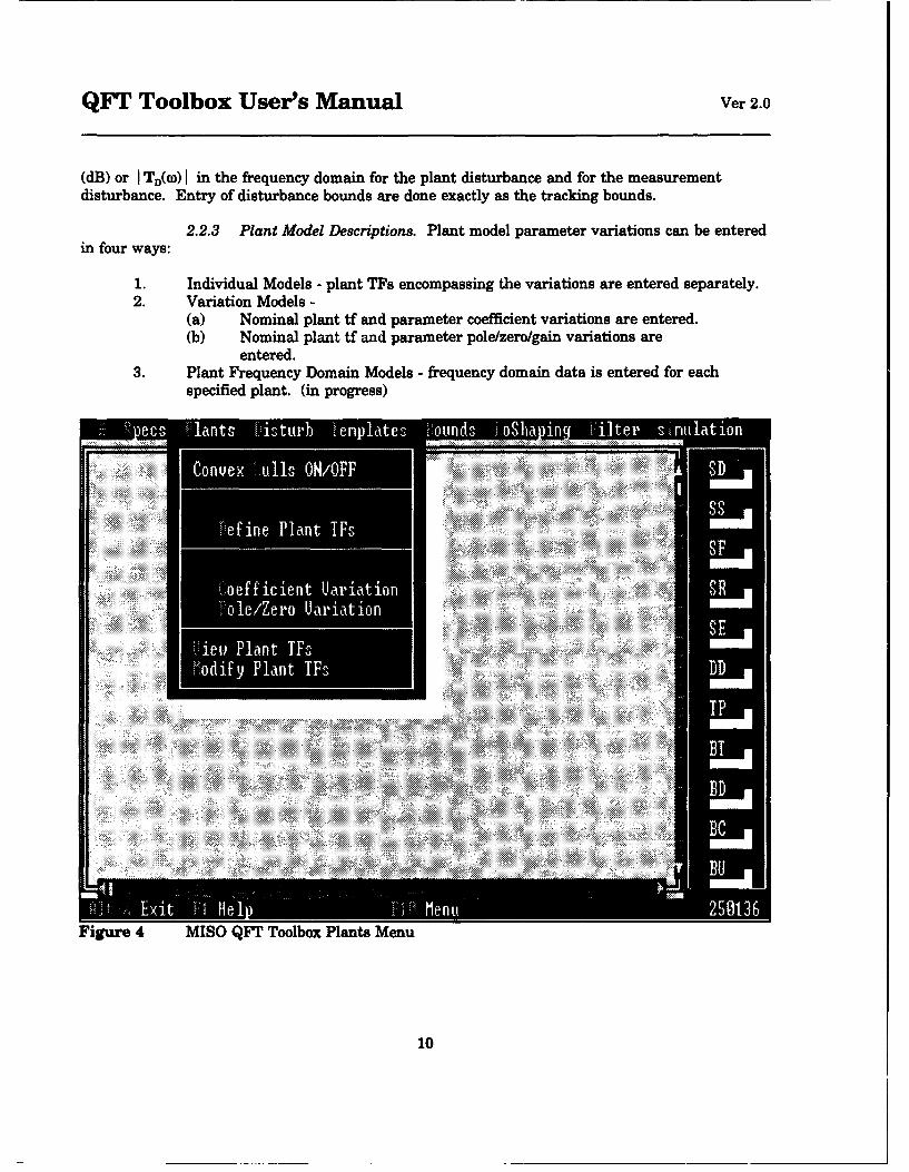
QFT Toolbox User's Manual Ver 2.0
(dB) or I TD(w) I in the frequency domain for the plant disturbance and for the measurementdisturbance. Entry of disturbance bounds are done exactly as the tracking bounds.
2.2.3 Plant Model Descriptions. Plant model parameter variations can be enteredin four ways:
1. Individual Models - plant TFs encompassing the variations are entered separately.2. Variation Models -
(a) Nominal plant tf and parameter coefficient variations are entered.(b) Nominal plant tf and parameter pole/zero/gain variations are
entered.3. Plant Frequency Domain Models - frequency domain data is entered for each
specified plant. (in progress)
Figure 4 MISO QFT Toolbox Plants Menu
10
QFT Toolbox User's Manual Ver 2.0
As can be seen from Figure 4, currently the first two methods are available withinICECAP.PC. With approach (1), the number of plants is first defined and then each plant isentered separately by specifying the gain and the zeros and poles in factored or unfactored formusing the standard ICECAP-PC input dialogue (order,gain, pole/zero-factored orcoefficients-polynomial). Each plant transfer function can be displayed and checked for properentry. Although not yet implemented, the user will have the ability to import plant models fromexternal ASCII files in a future release.
Approach (2a) requests the entry of the maximum and minimum for each numerator anddenominator coefficient. Currently the number of possible parameter variations is limited to fourbecause of memory size.
Approach (2b) requests the variation (max,min) in each zero, in each pole and in the plantgain. The user is requested to answer the following question concerning the polynomial form: "Doyou desire the transfer function roots (zeros/poles) to be represented as [s/a +1] or [s+a] for realroots or as [s2/(a2 + w2) + 2as/(a2 + w2) + 1] or [I2 + 2as + a2 + w2]?'
Observe that a user of this package can build a program that uses symbols to characterizethe coefficients or roots of the transfer function as related to some physical model. These symbolscan then be instantiated with specific values to generate the specific plants. In this way, the QFTtoolbox could be used to interactively design controllers for a variety of models in a givenapplication (automotive spring control, engine control, vehicle control, etc.).
2.2.3.1 Plant Transfer Function Models. First enter the number of plants tobe input (note that the 'tab' function highlights each section of the window). The plants are thenentered using the standard ICECAP-PC transfer function input dialog (num order, denom order,num gain, zeros, denom gain, poles) for each factored form.
2.2.3.2 Plant Parameter Variations. A nominal transfer function is enteredwith nominal parameters. The number of plant variations is requested. Then the positivevariation of each parameter (gain, zero, pole or coefficient) is entered in turn. The variation couldbe thought of as a uniform or a normal distribution. Depending upon the number of plantsrequested, a finite number (<= 625) of plant cases are defined.
2.2.4 Disturbance Models. Plant disturbance models are entered using thestandard ICECAP-PC format. The measurement disturbance model is not yet implemented. Gainis entered in real units not db.
2.2.5 Plant Template Generation. Because of plant uncertainty there exists a setof complex numbers {P(Oo)} for any frequency oa which are defined as plant templates. If individualplants are entered, then the package generates all the frequency domain points for each plant at agiven frequency. This data is then sorted by frequency to develop templates of uncertain plantresponse. The graphical structure of each template (one at each frequency) can also be displayedon the Nichols chart.
If the plant variation ranges are entered, then the package generates a convex hull aroundall the frequency domain points and selects only those point on the boundary of the hull forrepresenting the templates. This process reduces the number of plants since the maximumnumber of possible plants using the variation method is 625. This hull or template can also bedisplayed as a table or graphically on the Nichols chart.
2.2.6 Bounds. The tracking and disturbance bounds are generated in a similarmanner. However, in most cases, the disturbance bounds are generated from the disturbance
11
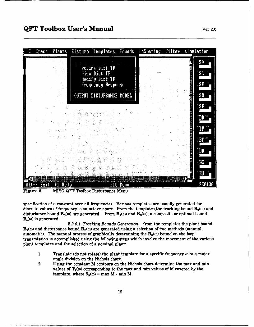
QFT Toolbox User's Manual Ver 2.0
Defin Dis ~IF I
Figure ISO QF'T oolbox Disturac Men
specification of a constant over all frequencies. Various templates are usually generated fordiscrete values of frequency (o an octave apart. From the templates,the tracking bound BR(co) anddisturbance bound Bd5w) are generated. From BR(w) and BD(w), a composite or optimal boundB0(co) is generated.
2.2.6.1 Tracking Bounds Generation. From the templates,the plant boundBR(o)) and disturbance bound Bd(o) are generated using a selection of two methods (manual,automatic). The manual process of graphically determining the BR(O) bound on the looptransmission is accomplished using the following steps which involve the movement of the variousplant templates and the selection of a nominal plant:
1. Translate (do not rotate) the plant template for a specific frequency 0o to a majorangle division on the Nichols chart.
2. Using the constant M contours on the Nichols chart determine the max and minvalues of TR(O) corresponding to the max and min values of M covered by thetemplate, where m(wo) = max M - min M.
12
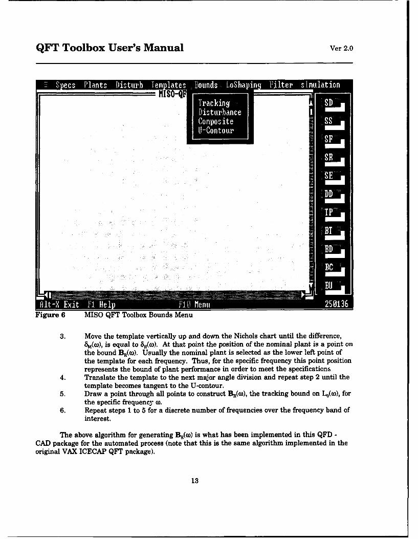
QFT Toolbox User's Manual Ver 2.0
Figure 6 MISO QFT Toolbox Bounds Menu
3. Move the template vertically up and down the Nichols chart until the difference,1ko(), is equal to 8 R(m). At that point the position of the nominal plant is a point on
the bound BR(w). Usually the nominal plant is selected as the lower left point ofthe template for each frequency. Thus, for the specific frequency this point positionrepresents the bound of plant performance in order to meet the specifications
4. Translate the template to the next major angle division and repeat step 2 until thetemplate becomes tangent to the U-contour.
5. Draw a point through all points to construct BR(wO), the tracking bound on L0(co), forthe specific frequency wo.
6. Repeat steps 1 to 5 for a discrete number of frequencies over the frequency band ofinterest.
The above algorithm for generating BR(co) is what has been implemented in this QFD -CAD package for the automated process (note that this is the same algorithm implemented in theoriginal VAX ICECAP QFT package).
13
QFT Toolbox User's Manual Ver 2.0
An educational interactive BR(to) generation mode is also available using movabletemplates on the Nichols Chart. Templates are entered for Nichols Chart display as tp#.dat.Template movement is possible with the use of the arrow keys. SR and 8. are displayed so thatthe student can move the template to the point where SR:5 S.. Points on the BR(co) curve at agiven frequency are stored with the press of the 'insert' key. The 'return' key provides exit frominteractive bounds generation.
2.2.6.2 Disturbance Bound Generation. The plant disturbancebound By(to) is determined by finding the minimum value of Lo(to) that satisfies the followingrelation:
P( < P°(e) Eq 10
across the range of plant uncertainty embodied in P(to). The tracking bounds can be listed andgraphed.
For the measurement disturbance the associated disturbance bound is found from theinequality using basically the same method:
I eo o(C) Eq 11
2.2.6.3 Composite Bound Generation. The combined or compositebound B. is generated by comparing the tracking and disturbance bounds and defining the highestboundary at each major angle division for a select number of frequencies which are an octaveapart. All bounds can be displayed on a Nichols chart for the synthesis of L4 in the next step.See Section 4.2 for information on the U-Contour.
2.2.6.4 U-Contours for Ultra-High Frequency. To help ensure that thesynthesized loop transmission Lo does not yield unstable roots or stable roots of the closed loopsystem close to the imaginary axis, an additional constraint is imposed. This constraint isexpressed as I V(1 + L) I < ML (the 82(w) constant) for all (o and all plant variations. In somecases this results in an ash can structure. The synthesized loop transmission must not penetratethis region on the Nichols chart.
The U-Contour or ultra-high frequency bound (UHFB) can be displayed in a table, graphand Nichols chart for the desired frequency range. It is based upon the desired phase angle andthe maximum variation of magnitude at high frequencies.
2.2.7 Loop Transmission Design. In order to develop the loop transmission, theLoop transmission, Lo, can be generated using a variety of techniques: manual, interactive, orautomatic. The loop shaping is accomplished by keeping the value of L4(o) above the compositebound B. at each distinct frequency while not violating the U-contour.
Currently, no CAD algorithm for completely automated design has been implemented. Aninitial L4 is selected and then modified by adding zeros and poles to meet the above criteria. A
14
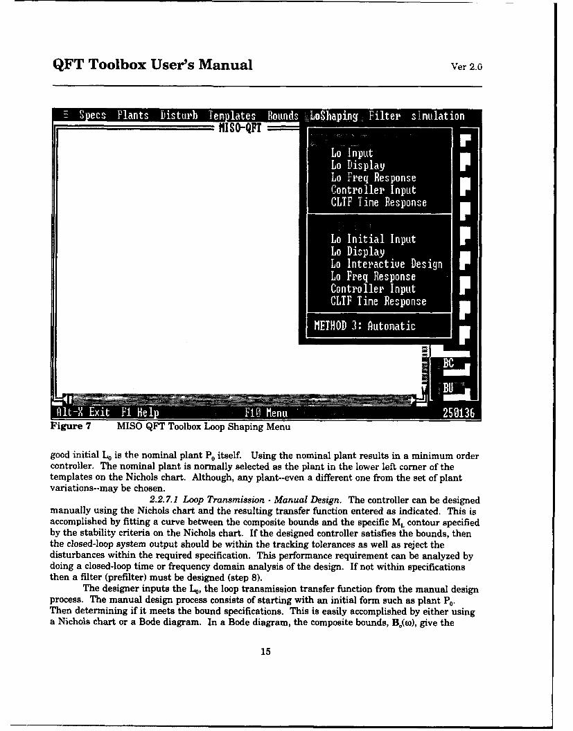
QFT Toolbox User's Manual Ver 2.0
""IS -QFT
Lo Inu
Figure~~~L 7re Responsole Lo Sapn Mn
Controller InptLo Inta Inpu
variatins--Lo beishosen2.2.~ ~ ~ ~ ~ ~ ~L 71LoTrnmsin-MnaDe Ign.theractvler Da besign e
Conrole Inu
Figure 7 MISO QFT Toolbox Loop Shaping Menu
good initial Lm is the nominal plant P0 itself Using the nominal plant results in a minimum ordercontroller. The nominal plant is normally selected as the plant in the lower left comer of thetemplates on the Nichols chart. Although, any plant--even a different one from the set of plantvariations--may be chosen.
2.2.7.1 Loop Transmission - Manual Design. The controller can be designedmanually using the Nichols chart and the resulting transfer function entered as indicated. This isaccomplished by fitting a curve between the composite bounds and the specific ML contour specifiedby the stability criteria on the Nichols chart. If the designed controller satisfies the bounds, thenthe closed-loop system output should be within the tracking tolerances as well as reject thedisturbances within the required specification. This performance requirement can be analyzed bydoing a closed-loop time or frequency domain analysis of the design. If not within specificationsthen a filter (prefilter) must be designed (step 8).
The designer inputs the L0, the loop transmission transfer function from the manual designprocess. The manual design process consists of starting with an initial form such as plant P0.Then determining if it meets the bound specifications. This is easily accomplished by either usinga Nichols chart or a Bode diagram. In a Bode diagram, the composite bounds, BJ(o), give the
15
QFT Toolbox User's Manual Ver 2.0
necessary magnitude and angle conditions for which L0 must be designed. Overdesign isminimized by placing L0 as close as possible to the bound. Zeros and poles are added to L4(W) inorder to meet and approach the composite bound. The U-contour corresponds to the phase marginbound on the Bode diagram while the composite bound Bok() on the Nichols chart defines theamplitude bound.
2.2.7.2 Loop Transmission - Interactive Design. After entering an initialL0(co), additional poles and zeros are added interactively. After each addition/subtraction of polesand zeros, an updated graph is generated. A recommended process is to locate the frequency atwhich the worst violation of the BO(W) bounds occurs. After finding this frequency, install one zeroin Lo(a)) for each 12 dB of violation at a frequency 1 octave (approx) below the violation frequency.An equal number of poles also needs to be installed 1 octave below this frequency to offset thezeros. Repeat this process until the B.(4) bounds are met while remaining outside and in closeproximity to the U-Contour to achieve minimum overdesign.
Poles are entered with 'shift p' and zeros are entered with 'shift z' commands. Entering the'return key' updates the Nichols chart with the new poles and zeros and stores the data to file.Use of the 'esc key' exits the procedure.
2.2.7.3 Loop Transmission - Automated Design. An automated design ofloop transmission is under current development. This process will provide the necessary tools forthe user to define a desired L4(o) at a distinct set of frequencies, a loop transmission orderconstraint, and a cost function such as a weighted least squares solution. The optimization processgenerates the transfer function coefficients that minimize the cost function.
2.2.7.4 The Controller. From Lo and the nominal plant, the compensator Gis generated from the equation L. = G * Po. This G is then employed as the robust controller. TheCLTF time responses can be generated for checking the design.
2.2.8 Filter Generation. The design of the controller G only guarantees thefrequency responses for any given P in (P) lies within a 8 R without regard to the actual position ofSR in the frequency domain. A prefilter translates the magnitude progression to lie between Buand BL frequency responses [D'Azzo, 1988:725].
In order to meet the original tracking frequency specifications for TR(w) = F.Lo()/(1 +Lo(co)), a fiter is employed to position the frequency domain closed-loop response within the desiredenvelope of TRU(o) and TR(ow). In some cases this is only a gain. The process consists of thefollowing 4 steps:
1. Place the nominal point of the plant template TP(W) on the point L4(0). DetermineT. and Tfi at that point using the M-contours. The entire perimeter (each plant)of the template must be inspected in order to determine the true T. and T.because the curvilinear nature of the ML Contour can be deceptive.
2. Obtain the values of TRu and TRL for various frequencies oo.3. From the values obtained in steps 1 and 2, plot [TRu - T.] and {TRL - T]J vs 0).
These values are the upper and lower bounds on the filter (prefilter). Thecommand Calculate Filter Transfer function generates this table.
4. Synthesis a filter that lies within the frequency plots by the use of straight lineapproximations. For a step forcing function, the following limit as s goes to zero (ortime goes to infinity) must be satisfied:
16
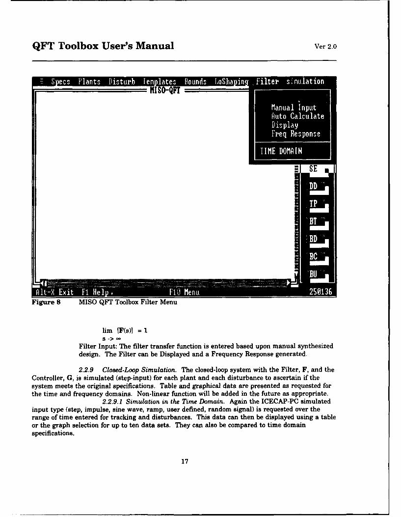
QFT Toolbox User's Manual Ver 2.0
Figure 8 MISO QFT Toolbox Filter Menu
uMn IF(s)l = 1
Filter Input: The filter transfer function is entered based upon manual synthesizeddesign. The Filter can be Displayed and a Frequency Response generated.
2.2.9 Closed.Loop Simulation. The closed-loop system with the Filter, F, and theController, G, is simulated (step-input) for each plant and each disturbance to ascertain if thesystem meets the original specifications. Table and graphical data are presented as requested forthe time and frequency domains. Non-linear function will be added in the future as appropriate.
2.2.9.1I Simulation in the Time Domain. Again the ICECAP-PC simulatedinput type (step, impulse, sine wave, ramp, user defined, random signal) is requested over therange of time entered for tracking and disturbances. This data can then be displayed using a tableor the graph selection for up to ten data sets. They can also be compared to time domainspecifications.
17
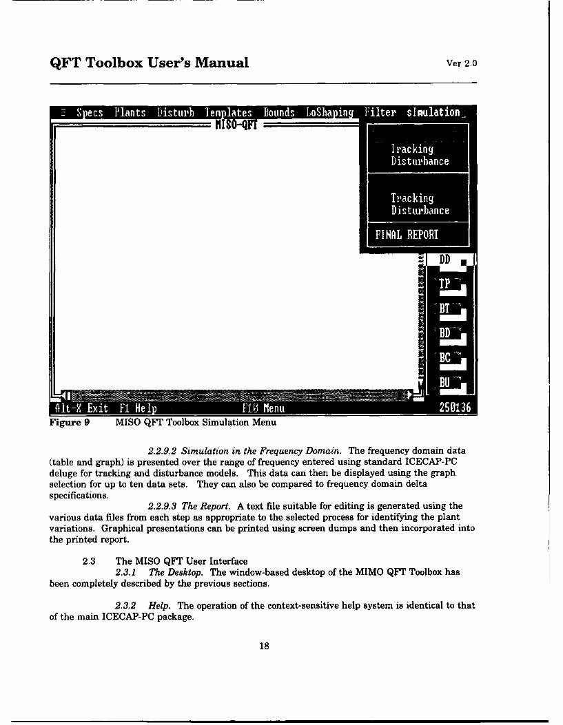
QFT Toolbox User's Manual Ver 2.0
HI SO-FT
Figure 9 MISO QFT Toolbox Simulation Menu
2.2.9.2 Simulation in the Frequency Domain. The frequency domain data(table and graph) is presented over the range of frequency entered using standard ICECAP-PGdeluge for tracking and disturbance models. This data can then be displayed using the graphselection for up to ten data sets. They can also be compared to frequency domain delta
specifications.2.2.9.3 The Report. A text file suitable for editing is generated using the
various data files from each step as appropriate to the selected process for identifying the plantvariations. Graphical presentations can be printed using screen dumps and then incorporated intothe printed report.
2.3 The MISO QFT User Interface2.3.1 The Desktop. The window-based desktop of the MIMO QFT Toolbox has
been completely described by the previous sections.
2.3.2 Help. The operation of the context-sensitive help system is identical to thatof the main ICECAP-PC package.
18
QFT Toolbox User's Manual Ver 2.0
2.3.3 The Toolbar. The operation of the toolbar is identical to that of the mainICECAP-PC package.
2.3.4 The Status Line. The operation of the status line is identical to that of themain ICECAP-PC package.
19
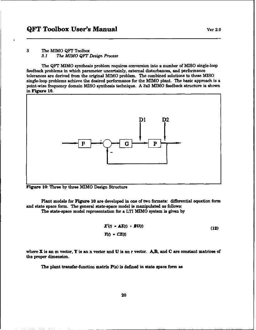
QFT Toolbox User's Manual Ver 2.0
3 The MIMO QFT Toolbox3.1 The MIMO QFT Design Process
The QFT MIMO synthesis problem requires conversion into a number of MISO single-loopfeedback problems in which parameter uncertainly, external disturbances, and performancetolerances are derived from the original MIMO problem. The combined solutions to these MISOsingle-loop problems achieve the desired performance for the MIMO plant. The basic approach is apoint-wise frequency domain MISO synthesis technique. A 3x3 MIMO feedback structure is shownin Figure 10.
D1 D2
Figure 10: Three by three MIMO Design Structure
Plant models for Figure 10 are developed in one of two formats: differential equation formand state space form. The general state-space model is manipulated as follows:
The state-space model representation for a LTI MIMO system is given by
X'(t) -AX(t) + BU(t) (12)
YWt) CX(t)
where X is an m vector, Y is an n vector and U is an r vector. AB, and C are constant matrices ofthe proper dimension.
The plant transfer-function matrix P(s) is defined in state space form as
20
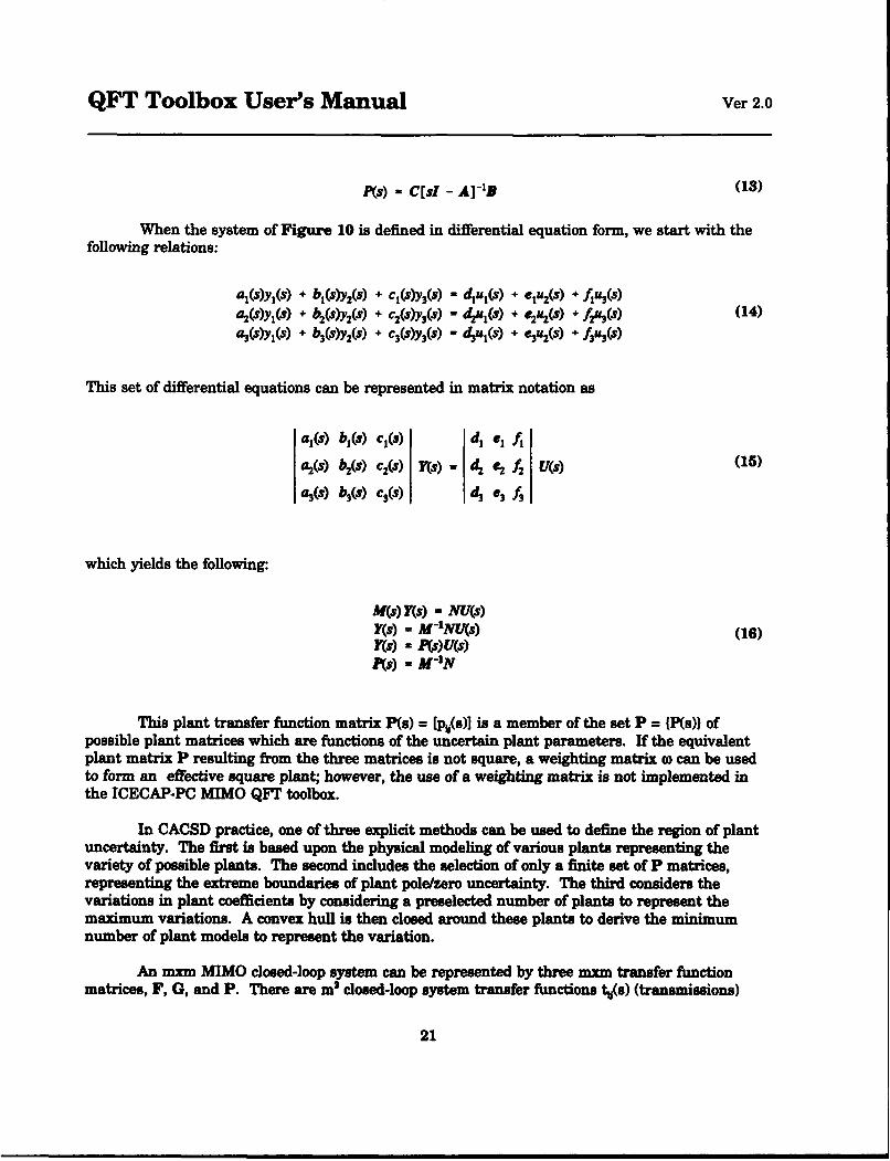
QFT Toolbox User's Manual Ver 2.0
P(s) - C[sl - A]'1 B (13)
When the system of Figure 10 is defined in differential equation form, we start with thefollowing relations:
aj(s)y,(s) + b1(s)y2(s) + cI(s)y3(s) - dju1 (s) + 1"2(S) + Iu3(s)a2(s)y1 (S) + b2(s)y(s) + c 2($)y3(s) - d2U(s) + . 2u2 (s) + fAu(s) (14)
a3(s)yI(s) + b3(s)yO(s) + c3(s)y3(s) - d3U1 (s) + e3A(s) + 3u3(s)
This set of differential equations can be represented in matrix notation as
a,(s) b,(s) c1(s) d, el f
a2(s) b2(s) C2(S) ¥(s) d2 e2 A U(s) (15)
a3(s) b3(S) c,(O) d3 e3 A
which yields the following:
M(s) Y(s) - NU(s)Y(s) = M-NI(s) (16)Y(s) - P(s)U(s)F(s) - M-'N
This plant transfer function matrix P(s) = [pv(s)] is a member of the set P = {P(s)) ofpossible plant matrices which are functions of the uncertain plant parameters. If the equivalentplant matrix P resulting from the three matrices is not square, a weighting matrix a can be usedto form an effective square plant; however, the use of a weighting matrix is not implemented inthe ICECAP-PC MIMO QFT toolbox.
In CACSD practice, one of three explicit methods can be used to define the region of plantuncertainty. The first is based upon the physical modeling of various plants representing thevariety of possible plants. The second includes the selection of only a finite set of P matrices,representing the extreme boundaries of plant pole/zero uncertainty. The third considers thevariations in plant coefficients by considering a preselected number of plants to represent themaximum variations. A convex hull is then closed around these plants to derive the minimumnumber of plant models to represent the variation.
An mxm MIMO closed-loop system can be represented by three mxm transfer functionmatrices, F, G, and P. There are m2 closed-loop system transfer functions N(s) (transmissions)
21
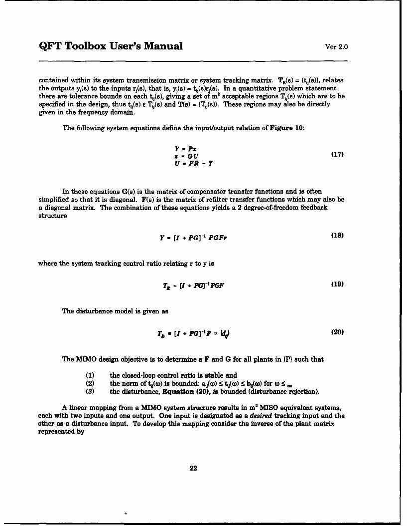
QFT Toolbox User's Manual Ver 2.0
contained within its system transmission matrix or system tracking matrix. TR(s) = ft•(s)}, relatesthe outputs y1(s) to the inputs r,(s), that is, yi(s) = tj(s)r(s). In a quantitative problem statementthere are tolerance bounds on each t,(s), giving a set of m2 acceptable regions T,(s) which are to bespecified in the design, thus t%(s) F T,(s) and T(s) = fT•(s)). These regions may also be directlygiven in the frequency domain.
The following system equations define the input/output relation of Figure 10:
Y = PXx w GU (17)U=FR - Y
In these equations G(s) is the matrix of compensator transfer functions and is oftensimplified so that it is diagonal. F(s) is the matrix of refilter transfer functions which may also bea diagonal matrix. The combination of these equations yields a 2 degree-of-freedom feedbackstructure
Y - [I + PG]-1 PGFr (18)
where the system tracking control ratio relating r to y is
T= = [I + PG-IPGF (19)
The disturbance model is given as
TD n [I + PG]-'P= - jJ (20)
The MIMO design objective is to determine a F and G for all plants in (P) such that
(1) the closed-loop control ratio is stable and(2) the norm of t%(0o) is bounded: a%((o) < %(W) < b,((o) for co <(3) the disturbance, Equation (20), is bounded (disturbance rejection).
A linear mapping from a MIMO system structure results in m2 MISO equivalent systems,each with two inputs and one output. One input is designated as a desired tracking input and theother as a disturbance input. To develop this mapping consider the inverse of the plant matrixrepresented by
22
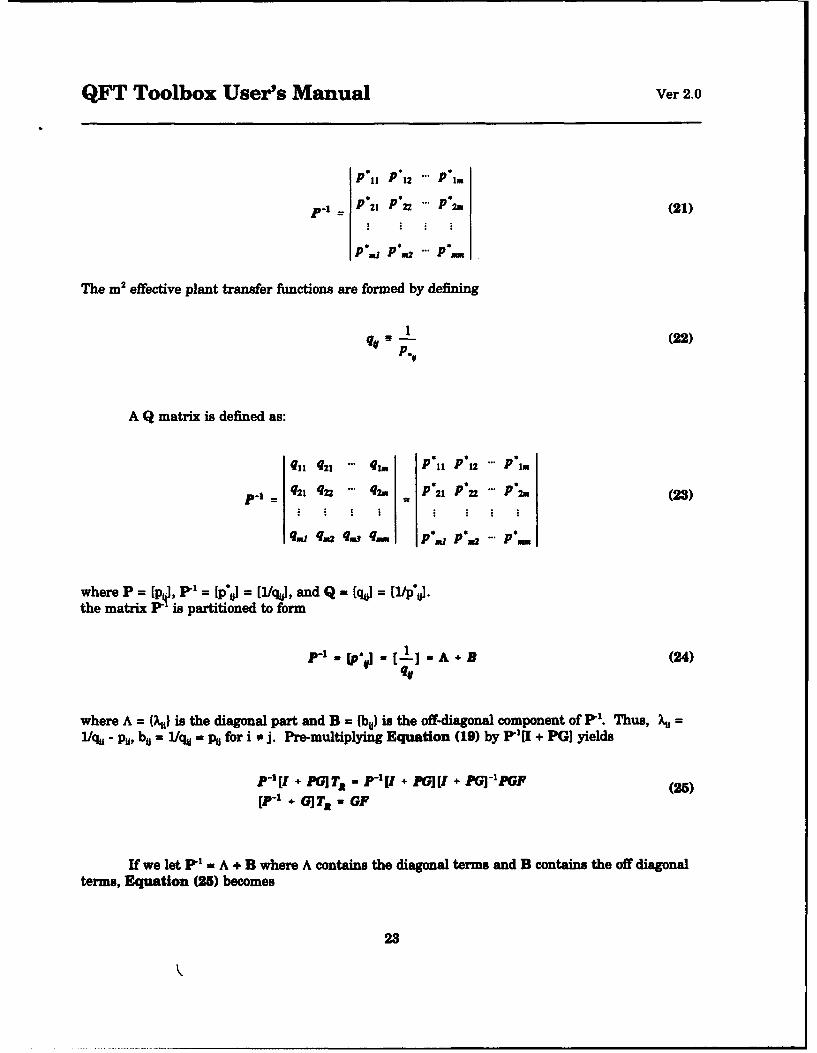
QFT Toolbox User's Manual Ver 2.0
Pol P' 12 P'Lra
p-I _ P021 P' 22 P'2 (21)
P*,1 P "2 P*.
The m2 effective plant transfer functions are formed by defining
q 1 - 1 (22)
A Q matrix is defined as:
qj, q2I qj1 Poll P'12 P'1.
p-I = 2 q22 q2 . = P*21 P'- P's. (23)
q.d q.2 q.3 q.- p*.d p*., .p*..
where P = , P 1 = f[p*4] = [1/qj], and Q = [Q]i [1/p10].the matrix F is partitioned to form
P-1. rp'j1 [1] A + B (24)qV
where A = {Au) is the diagonal part and B = {bu) is the off-diagonal component of P'. Thus, .=1/A - pi, bm = 1/% = PM for i o j. Pre-multiplying Equation (19) by F•1[I + PGI yields
P-'[ + IqT,, - P-1[I ÷ PGJ[I + PGM'ZPGP (25)
[P-1 + GITjt - GP
If we let 1 m = A + B where A contains the diagonal terms and B contains the off diagonalterms, Equation (25) becomes
23
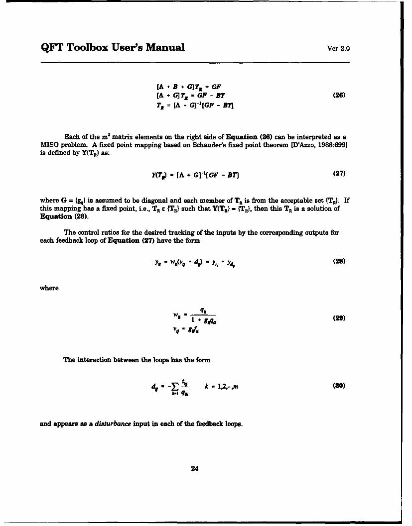
QFT Toolbox User's Manual Ver 2.0
[A+5 +GQTR = GF[A + G]TR = GF - BT (26)TR = [A + G]-'[GF - BT]
Each of the m2 matrix elements on the right side of Equation (26) can be interpreted as aMISO problem. A fixed point mapping based on Schauder's fixed point theorem [D'Azzo, 1988:699]is defined by Y(TR) as:
Y(T,) = [A + G]-'[GF - BT] (27)
where G = {g•} is assumed to be diagonal and each member of T. is from the acceptable set {TRI. Ifthis mapping has a fixed point, i.e., TR e {TR} such that Y(TR) = {TR}, then this TR is a solution ofEquation (26).
The control ratios for the desired tracking of the inputs by the corresponding outputs foreach feedback loop of Equation (27) have the form
yv = w,(v, + do - y,, + y, (28)
where
" + g- m (29)
vo- gim
The interaction between the loops has the form
k-l - - ,...rV (so)
kof qft
and appears as a disturbance input in each of the feedback loops.
24
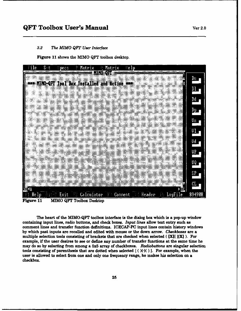
QFT Toolbox User's Manual Ver 2.0
3.2 The MIMO QFT User Interface
Figure 11 shows the MIMO QFT toolbox desktop.
F l .... ý, ec Mati r xM t ix i ie ilp! ~i!iiii.:i~
H NJN-FT Too Bo ntalled and Active
Figure 11 MIMO QFT Toolbox Desktop
The heart of the MIMO-QFT toolbox interface is the dialog box which is a pop-up windowcontaining input lines, radio buttons, and check boxes. Input lines allow text entry such ascomment lines and transfer function definitions. ICECAP-PC input lines contain history windowsby which past inputs are recalled and edited with mouse or the down arrow. Checkboxes are amultiple selection tools consisting of brackets that are checked when selected ( XI][ I[XI ). Forexample, if the user desires to see or define any number of transfer functions at the same time hemay do so by selecting from among a 5x5 array of checkboxes. Radiobuttons are singular selectiontools consisting of parenthesis that are dotted when selected [ ( )(9( ) 1. For example, when theuser is allowed to select from one and only one frequency range, he makes his selection on acheckbox.
25
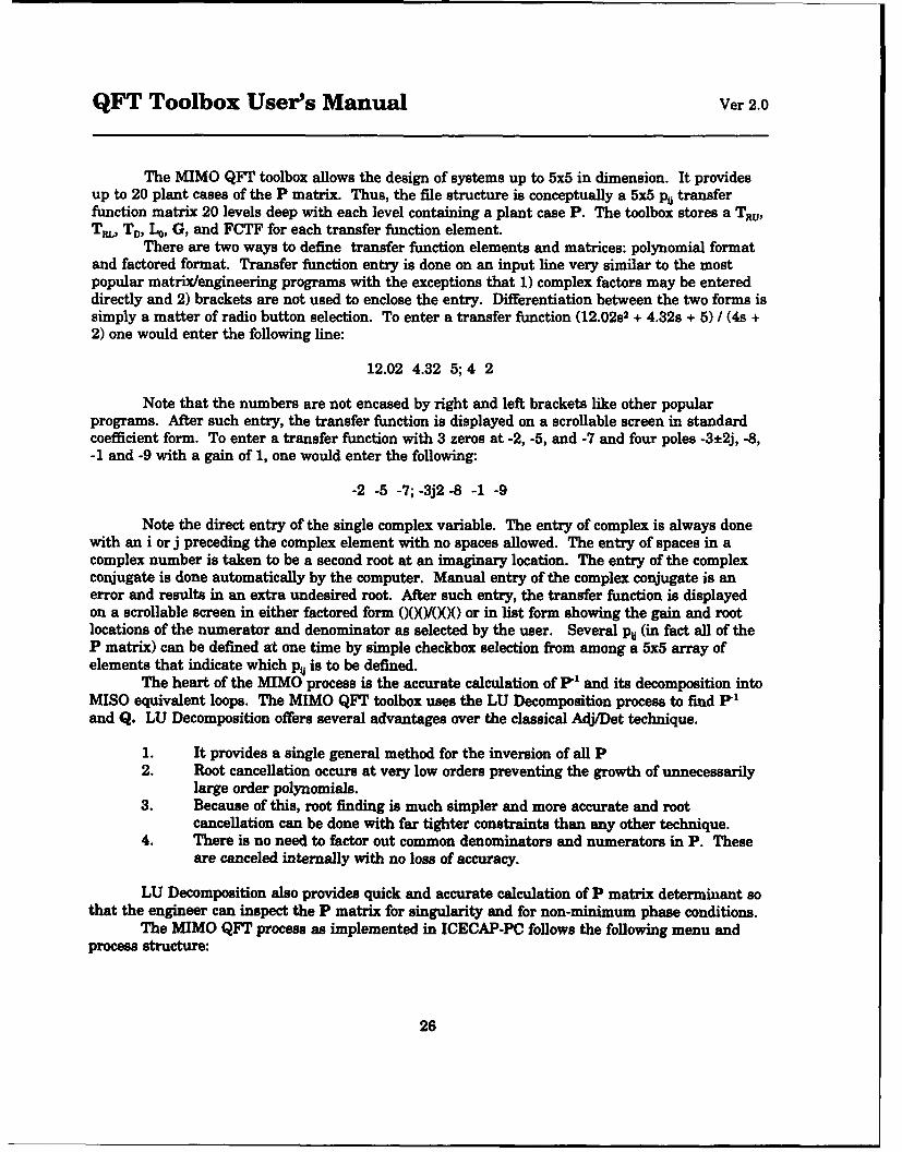
QFT Toolbox User's Manual Ver 2.0
The MIMO QFT toolbox allows the design of systems up to 5x5 in dimension. It providesup to 20 plant cases of the P matrix. Thus, the file structure is conceptually a 5x5 p, transferfunction matrix 20 levels deep with each level containing a plant case P. The toolbox stores a TRu,TRL, TD, L4, G, and FCTF for each transfer function element.
There are two ways to define transfer function elements and matrices: polynomial formatand factored format. Transfer function entry is done on an input line very similar to the mostpopular matrix/engineering programs with the exceptions that 1) complex factors may be entereddirectly and 2) brackets are not used to enclose the entry. Differentiation between the two forms issimply a matter of radio button selection. To enter a transfer function (12.02s 2 + 4.32s + 5) / (4s +2) one would enter the following line:
12.02 4.32 5; 4 2
Note that the numbers are not encased by right and left brackets like other popularprograms. After such entry, the transfer function is displayed on a scrollable screen in standardcoefficient form. To enter a transfer function with 3 zeros at -2, -5, and -7 and four poles -3±2j, -8,-1 and -9 with a gain of 1, one would enter the following:
-2 -5 -7; -3j2 -8 -1 -9
Note the direct entry of the single complex variable. The entry of complex is always donewith an i or j preceding the complex element with no spaces allowed. The entry of spaces in acomplex number is taken to be a second root at an imaginary location. The entry of the complexconjugate is done automatically by the computer. Manual entry of the complex conjugate is anerror and results in an extra undesired root. After such entry, the transfer function is displayedon a scrollable screen in either factored form (XX)/X) or in list form showing the gain and rootlocations of the numerator and denominator as selected by the user. Several p. (in fact all of theP matrix) can be defined at one time by simple checkbox selection from among a 5x5 array ofelements that indicate which p, is to be defined.
The heart of the MIMO process is the accurate calculation of F 1 and its decomposition intoMISO equivalent loops. The MIMO QFT toolbox uses the LU Decomposition process to find P'and Q. LU Decomposition offers several advantages over the classical Adj/Det technique.
1. It provides a single general method for the inversion of all P2. Root cancellation occurs at very low orders preventing the growth of unnecessarily
large order polynomials.3. Because of this, root finding is much simpler and more accurate and root
cancellation can be done with far tighter constraints than any other technique.4. There is no need to factor out common denominators and numerators in P. These
are canceled internally with no loss of accuracy.
LU Decomposition also provides quick and accurate calculation of P matrix determinant sothat the engineer can inspect the P matrix for singularity and for non-minimum phase conditions.
The MIMO QFT process as implemented in ICECAP-PC follows the following menu andprocess structure:
26

QFT Toolbox User's Manual Ver 2.0
3.2.1 File.
HI No QFltailed and Active
Figure 12 MIMO QFT Toolbox File Menu
Log File On: Activates the ICECAP-PC log file. All subsequent information displayed toscreen is also sent to the log file. The log file is a text file named LOGFILE.TXT and assuch can be viewed, printed or edited with any good text editor.
Log File Off. Turns log file off.
DOS Shell: Provides Temporary exit to DOS. Once in the DOS environment, return to theICECAP-PC MIMO QFT program is initiated with the 'Exit' DOS command. Caution: Donot attempt to edit an active log file by using this option.
Exit: Exits the ICECAP-PC MIMO QFT toolbox.
27

QFT Toolbox User's Manual Ver 2.0
3.2.2 Set.
Figure 13 MIMO QFT Toolbox Set Menu
Clear Display: Clears the screen.
CommentLine: Presents direct entry of comments into the design session. Comments canbe up to 132 characters long. If the log fie is active, comments are also sent to it.
Header: Provides a dialog box to record the user/student name, title and other headerinformation that should appear on top of log files. The header information is saved to diskand recalled each time the log file is turned on with the header option enabled.
View Options: Allows user to customize the session including the selection of highresolution screens, Number of decimal places displayed, fixed decimals or scientific notationdisplay selection, and complex letter (i or j) selection.
28
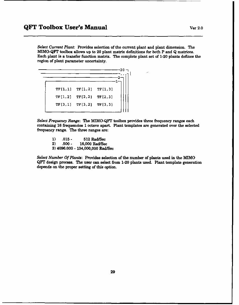
QFT Toolbox User's Manual Ver 2.0
Select Current Plant: Provides selection of the current plant and plant dimension. TheMIMO-QFT toolbox allows up to 20 plant matrix definitions for both P and Q matrices.Each plant is a transfer function matrix. The complete plant set of 1-20 plants defines theregion of plant parameter uncertainty.
20-
-2-
TF[1,1] TF[1,2] TF[1,3]
TF[1,2J TF[2,2J TF(2,3]
TF[3,1] TF[3,2] TF[3,33
Select Frequency Range: The MIMO-QFT toolbox provides three frequency ranges eachcontaining 16 frequencies 1 octave apart. Plant templates are generated over the selectedfrequency range. The three ranges are:
1) .015 - 512 Rad/Sec2) .500 - 16,000 Rad/Sec3) 4096.000 - 134,000,000 Rad/Sec
Select Number Of Plants: Provides selection of the number of plants used in the MIMOQFT design process. The user can select from 1-20 plants used. Plant template generationdepends on the proper setting of this option.
29
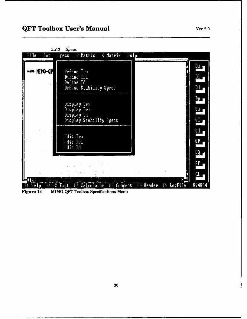
QFT Toolbox User's Manual Ver 2.0
3.2.3 Specs.
Nw*f iII 11%
Figure 4 MIMO fTn Stoolbox SpecifctossMn
F30
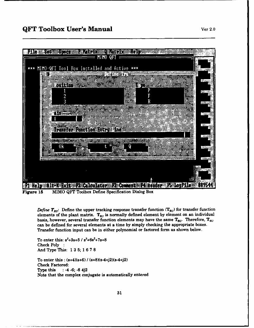
QFT Toolbox User's Manual Ver 2.0
.... .~ ...-
Figure 15 MIMO QFT Toolbox Define Specification Dialog Box
Define TRU: Define the upper tracking response transfer function (TRu) for transfer functionelements of the plant matrix. TRu is normally defined element by element on an individualbasis, however, several transfer function elements may have the same TRu. Therefore, TRu
can be defined for several elements at a time by simply checking the appropriate boxes.Transfer function input can be in either polynomial or factored form as shown below.
To enter this: s2+3s+5 / s3+6s2+7s+8Check Poly :And Type This: 13 5; 16 7 8
To enter this : (s+4Xs+6) / (s+8Xs-4+j2Xs-4+j2)Check Factored:Type this : -4 -6; -8 4j2Note that the complex conjugate is automatically entered
31
QFT Toolbox User's Manual Ver 2.0
Display TR.: Display TRu for any p. element/elements desired.
Edit TRzc: Edit TRu for any transfer function element of the plant matrix.
Define TSL: Define the lower tracking response transfer function (TRL) for transfer functionelements of the plant matrix. TRL cannot be defined for off-diagonal elements. TRL isnormally defined element by element on an individual basis, however, several transferfunction elements may have the same TRL. Therefore, TRL can be .. ,"fined for severaldiagonal elements at a time by simply checking the appropriate boxes. Transfer functioninput can be in either polynomial or factored form as shown below.To enter this: s2+3s+5 / s3+6s2+7s+8Check Poly :And Type This: 13 5; 16 7 8
To enter this : (s+4Xs+6) / (s+8Xs-4+j2Xs-4+j2)Check Factored:Type this : -4 -6; -8 4j2Note that the complex conjugate is automatically entered
Display Ts,: Display TRL for any PN element(s) desired. Since TRL is undefined for off-diagonal elements, the display of such TRL is disallowed.
Edit Tjm: Edit TRL for any transfer function element of the plant matrix.
Define TD" Define the disturbance tracking response transfer function (TD) for transferfunction elements of the plant matrix. TD is normally defined element by element on anindividual basis, however, several transfer fimction elements may have the same TD.
Therefore, TD can be defined for several elements at a time by simply checking theappropriate boxes. Transfer function input can be in either polynomial or factored form asshown below. However, it is common practice to simply define TD as some constant (i.e., .1for -20db)
To enter this: s2+3s+5 / sl+6s'+7s+8Check Poly :And Type This: 135;1678
To enter this : (s+4Xs+6) / (s+8Xs-4+j2Xs-4+j2)Check Factored:Type this : -4 -6; -8 4j2Note that the complex conjugate is automatically entered
Display Tz" Display Tb for any p. element(s) desired.
Edit TD: Edit TD for any transfer function element in the plant matrix.
Define Stability Specs: Stability specifications may be defined as either a phase margin (y),a ML contour, or a peak overshoot(M,). Specifications are entered one for each row in the
32

QFT Toolbox User's Manual Ver 2.0
design and multiple rows may be define simultaneously. The entry of gain margin isspecifically disallowed because 1) the sensitivity of phase margin with respect to gainmargin and 2) the ill conditioned nature of calculating the phase margin given a gainmargin which is error prone. Using any definition provided results in the printing of allspecs.
Display Stability Specs: Display stability specifications for any number of row(s) of the Pmatrix. The display will show phase margin, peak overshoot, Ml contour, and gain margin.
3.2.4 Plants.
-HtI•O-PT Tool -,"---'l"
Plant~ IIIet.
Figure 16 MIMO QFT Toolbox Plant Matrix Menu
Define Plant Elements p: Define the plant transfer function p, for transfer functionelements of the plant matrix P. p4 is normally defined element by element on anindividual basis, however, several transfer function elements may have the same definition.Therefore, p, can be defined for several elements at a time by simply checking the
appropriate boxes. Transfer function input can be in either polynomial or factored form asshown below. The current P is indicated in the dialog box and may be set using the Select
33

QFT Toolbox User's Manual Ver 2.0
Figure 17 MIMO QFT Toolbox Plant Matrix Definition Dialog Box
Current Plant option.
To enter this: s2+3s+5 / s3+6S2+7s+8Check Poly :And Type This: 13 5; 16 7 8
To enter this : (s+4Xs+6) / (s+8)(s-4+j2)(s-4+j2)Check Factored:Type this : -4 -6; -8 4j2Note that the complex conjugate is automatically entered
Define Plant Variation: Provides an automated method for generating 20 plant cases. Theuser defines two transfer functions at the minima and maxima in variation for any givenplant p,. Entry is allowed in polynomial or factored form by selection. The MIMO-QFTtoolbox will automatically generate 125 plant cases for each plant element p,, envelop theseplants (p,) with a convex hull, and choose 20 plants on its perimeter.
34
QFT Toolbox User's Manual Ver 2.0
Copy Plant Matrix P:
Display Plant Elements p: Provides for the display of 1-25 plants pý in a given plant P asselected in Select Current Plant (described above).
Display Plant Matrix P: Allows the rapid display of all p, in a given plant case P. This isa separate menu item from the Display Plants option because the selection of several p. ina matrix can be a time consuming task. Radio button selection allows selection of thedesired plant case and P dimension.
Edit Plant Elements p:
Find Plant Determinant: Calculates and displays the determinant for a selected P. P ischosen via radiobutton selection. In the QFT design process, all P must be checked fornon-singularity and for minimum phase conditions. Calculation of the determinant is viaLU Decomposition.
High Freq Sign Check: Calculates and displays the sign of diagonal elements pi of P forall plant P cases.
35

QFT Toolbox User's Manual Ver 2.0
3.2.5 Q Matrix.
S1I11-QFT Tool Box Installe
i~ruu~iRl1i1 11s1
Figure 18 MIMO QFT Toolbox Q Matrix Menu
Define Plant Elements q: Define the plant transfer function q• for transfer functionelements of the plant matrix Q. THE DIRECT DEFINITION OF Q IS AN ALTERNATIVETO THE NORMAL INVERSION OF P. %. is normally defined element by element on anindividual basis, however, several transfer function elements may have the same definition.Therefore, %. can be defined for several elements at a time by simply checking the
appropriate boxes. Transfer function input can be in either polynomial or factored form asshown below. The current P is indicated in the dialog box and may be set using the SelectCurrent Plant option.
To enter this: s2+3s+5 / S8+6S2+7s+8Check Poly :And Type This: 13 5; 16 7 8
To enter this : (s+4Xs+6) / (s+8Xs-4+j2Xs-4+j2)
36
QFT Toolbox User's Manual Ver 2.0
Check Factored:Type this : -4 -6; -8 4j2Note that the complex conjugate is automatically entered
Form Q Matrix: Inverts the selected matrix P via LU decomposition and then reciprocatesthe elements of P4 to form the matrix Q.
Verify Plant Inversion: Multiplies P x PF in order to verify the accuracy of the inversionprocess. Ideally in the absence of zero roundoff error, the result will be an identity matrix.In practice, finite roundoff error is detected via this process. Scientific notation displayshould be used with this option to detect low levels of roundoff.
Check Diagonal Dominance: Calculates the magnitude of each P in a selected P viaLAHospitals rule and displays the result along with an analysis as to the diagonaldominance of the plant Q. A dialog box provides radiobutton selection among 20 Q.
Display Plant Elements q: Provides a dialog box with checkbox input for the display of 1-25 plants q% in a given plant Q as selected in Select Current Plant (described above).
Display Plant Matrix Q: Allows the rapid display of all %. in a given plant case Q. This is"a separate menu item from the Display Plants option because the selection of several q6 in"a matrix can be a time consuming task. Radio button selection allows selection of thedesired plant case and Q dimension.
Edit Plant Elements q:
37

QFT Toolbox User's Manual Ver 2.0
4 Design Examples4.1 MIMO QFT Design Example
Students NameTeachers NameClass
This log provides demonstration of the entry modes and operation of: MIMO-QFT toolbox functions and operation.
: Step 1: Define T.., ., and TD for plant P. Only plant P1 is shown below:: Note that in this example, T'u and Tj, are the same for all rows.
MIMO T" [1,1]
1.8896 (s + 12.0000)
(s + 2.2857 ± j4.1775)
MIMO T,, [2,2]
1.8896 (s + 12.0000)
(s + 2.2857 ± j4.1775)
MIMO T,, [3,3]
1.8896 (s + 12.0000)
(s + 2.2857 ± j4.1775)
: I't for off diagonal elements is defined for all off diagonal plants as:
MIMO Tw [1,21
0.1000
1.0000
MIMO Tm (1,3]
0.1000
1.0000
MIMO T' (2,11
0.1000
1.0000
MIMO Tw (2,3]
0.1000
1.0000
MIMO Tw [3,1]
0.1000
1.0000
MIMO T' [3,21
0.1000
1.0000
38
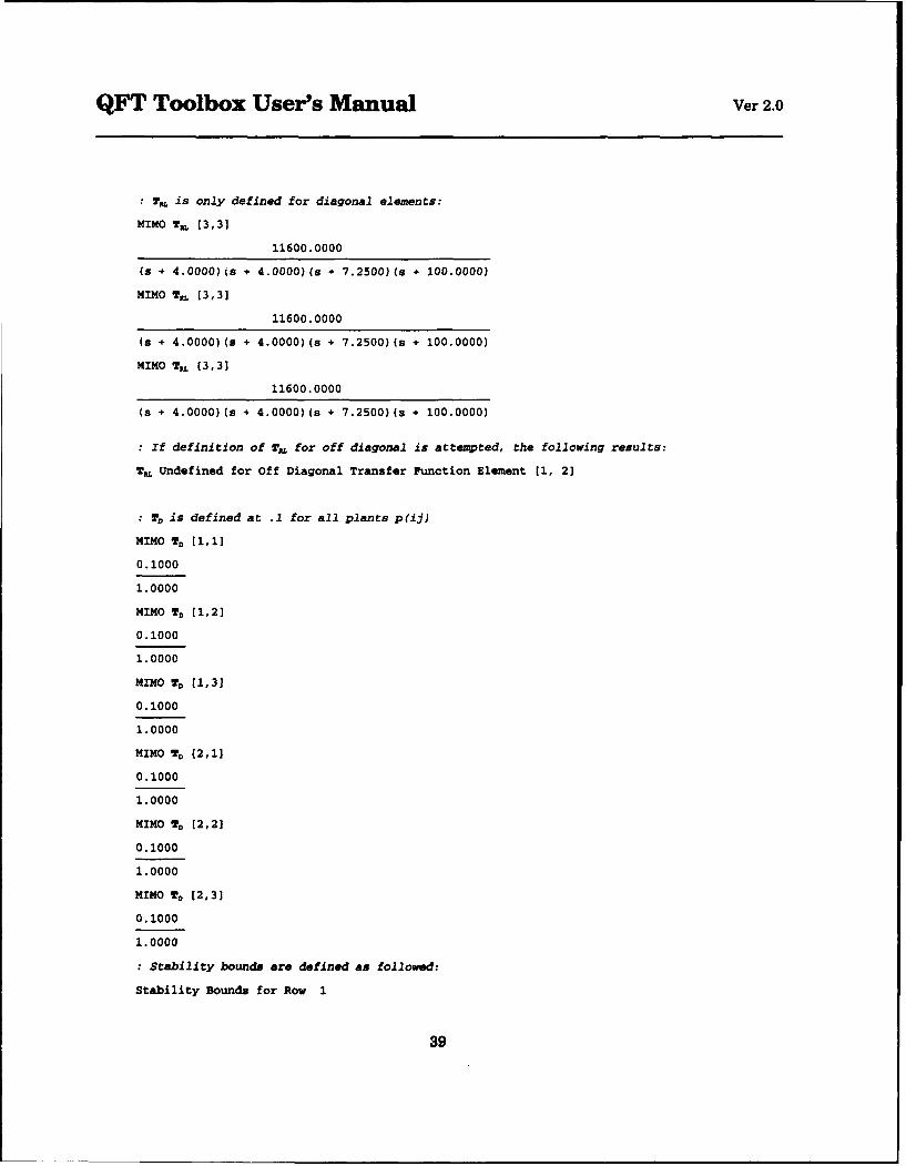
QFT Toolbox User's Manual Ver 2.0
: Tp is only defined for diagonal elements:
MIM0 T,, [3, 31
11600.0000
(s + 4.O000)(s + 4.0000)(s + 7.2500)(s + 100.0000)
MIMO Tn [3,3]
11600.0000
(s + 4.0000)(s + 4.0000)(s + 7.2500)(s + 100.0000)
MIM0 T,, [ 3, 3]
11600.0000
(s + 4.0000)(s + 4.0000)(s + 7.2500)(s + 100.0000)
: If definition of 7,, for off diagonal is attempted, the following results:
T! Undefined for Off Diagonal Transfer Function Element [1, 2]
: T is defined at .1 for all plants p(ij)
MIM0 T, [i,1]
0.1000
1.0000
MIMO T, [1,2]
0.1000
1.0000
MIMO TD [1,3]
0.1000
1.0000
MIM0 TD (2,1]
0.1000
1.0000
MIMO T,, [2,2]
0.1000
1.0000
MIO T, [2,3]
0.1000
1.0000
: Stability bounds are defined as followed:
Stability Bounds for Row 1
39
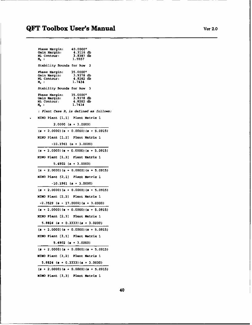
QFT Toolbox User's Manual Ver 2.0
Phase Margin: 40.00000Gain Margin: 4.3116 dbML Contour: 3.8387 dbM, : 1.5557
Stability Bounds for Row 2
Phase Margin: 35.00000Gain Margin: 3.9378 dbML Contour: 4.8282 dbM, : 1.7434
Stability Bounds for Row 3
Phase Margin: 35.00000Gain Margin: 3.9378 dbML Contour: 4.8282 dbMp : 1.7434
- Plant Case P, is defined as follows:
MIMO Plant (1,1] Plant Matrix 1
2.0000 (s + 3.0000)
(s + 2.0000) (s + 0.0000)(s + 5.0915)
MIMO Plant [1,2] Plant Matrix 1
-10.1961 (s + 3.0000)
(s + 2.0000)(s + 0.0000)(a + 5.0915)
MIMO Plant [1,3] Plant Matrix 1
5.4902 (a + 3.0000)
(s + 2.0000) ( + 0.0000)(a + 5.0915)
MIMO Plant [2,1] Plant Matrix 1
-10.1961 (a + 3.0000)
(a + 2.0000) (a + 0.0000)(s + 5.0915)
MIMO Plant [2,2] Plant Matrix 1
-2.3529 (a - 17.0000)(a + 3.0000)
(z + 2.0000) (a + 0.0000)(s + 5.0915)
MIMO Plant [2,3] Plant Matrix 1
5.8824 (a + 0.3333)(s + 3.0000)
(a + 2.0000) ( + 0.0000)(a + 5.0915)
MIMO Plant [3,1] Plant Matrix 1
5.4902 (a + 3.0000)
(a + 2.0000) (a + 0.0000)(a + 5.0915)
MIMO Plant (3,2] Plant Matrix 1
5.8824 (a + 0.3333)(s + 3.0000)
(a + 2.0000) (s + 0.0000)(s + 5.0915)
MIMO Plant [3,3] Plant Matrix 1
40
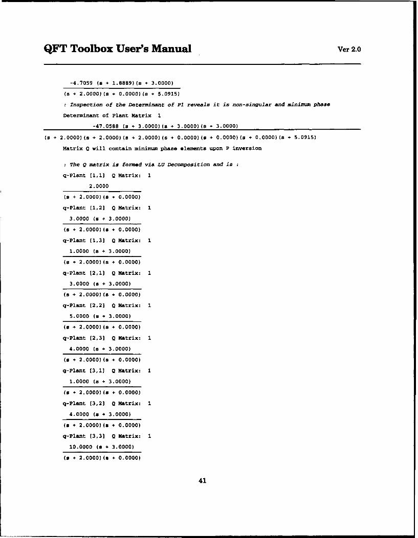
QFT Toolbox User's Manual Ver 2.0
-4.7059 (s + 1.8889)(s + 3.0000)
(s + 2.0000)(s + O.0000(s + 5.0915)
: Inspection of the Determinant of P1 reveals it is non-singular and minimum phase
Determinant of Plant Matrix 1
-47.0588 (s + 3.0000)(s + 3.0000)(s + 3.0000)
(s + 2.0000)(s + 2.0000)(s + 2.0000)(s + 0.0000)(s + 0.0000)(s + 0.0000)(s + 5.0915)
Matrix Q will contain minimum phase elements upon P inversion
: The Q matrix is formed via LU Decomposition and is
q-Plant [1,1] Q Matrix: 1
2.0000
(s + 2.0000)(s + 0.0000)
q-Plant [1,2] Q Matrix: 2
3.0000 (s + 3.0000)
(a + 2.0000)(s + 0.0000)
q-Plant [1,3] Q Matrix: 2
1.0000 (s + 3.0000)
(a + 2.0000)(s + 0.0000)
q-Plant [2,1] Q Matrix: 2
3.0000 (s + 3.0000)
(s + 2.0000) (s + 0.0000)
q-Plant [2,2] Q Matrix: 1
5.0000 (a + 3.0000)
(a + 2.0000) (a + 0.0000)
q-Plant (2,3] Q Matrix: 1
4.0000 (a + 3.0000)
(s + 2.0000)(a + 0.0000)
q-Plant (3,1] Q Matrix: 1
1.0000 (a + 3.0000)
(s + 2.0000)(a + 0.0000)
q-Plant [3,2] Q Matrix: 1
4.0000 (a + 3.0000)
(a + 2.0000)(s + 0.0000)
q-Plant (3,3] Q Matrix: 1
10.0000 (a + 3.0000)
(a + 2.0000)(8 + 0.0000)
41
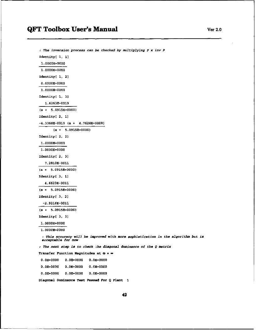
QFT Toolbox User's Manual Ver 2.0
: The inversion process can be checked by multiplying P x inv P
Identity[ 1, 1]
1.0000E+0000
1.0000E÷0000
Identity[ 1, 2)
0.0000E+0000
1.o000E+0000
Identity[ 1, 31
1.6263E-0019
(s + 5.0915E+0000)
Identity[ 2, 1]
-4.3368E-0019 (a + 4.7624E+0008)
(s + 5.0915E+0000)
Identity[ 2, 2]
1.0000+E0000
1.OOOOE+0000
Identity[ 2, 3]
7.2810E-0011
(s + 5.0915E+0000)
Identity[ 3, 1]
4.6623E-0011
(s + 5.0915E+0000)
Identity[ 3, 21
-2.9216E-0011
(s + 5.0915E+0000)
Identity[ 3, 3]
1.OOOOE+0000
1.00001+0000
: This accuracy will be imroved with more sophistication in the algorithm but isacceptable for now
The next step Is to check -he diagonal dominance of the Q matrix
Transfer Function Magnitudes at w =
0.OE+0000 0.0E+0000 0.OE+0000
0.0E+0000 0.0E+0000 0.01+0000
0.0E+0000 0.01+0000 0.0E+0000
Diagonal Dominance Test Passed For Q Plant 1
42
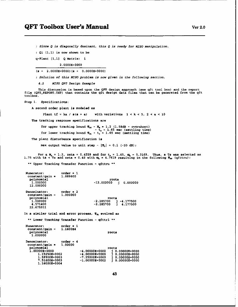
QFT Toolbox User's Manual Ver 2.0
: Since Q is diagonally dominant, this Q is ready for MISO manipulation.
: Q1 (1,1) is now shown to be
q-Plant [1,1] Q Matrix: 1
2.OOOOE+0000
(s + 2.OOOOE+0000)(s + 0.OOOOE+0000)
* Solution of this MISO problem is now given in the following section.
4.2 MISO QFT Design Example
This discussion is based upon the QFT design approach (see qft tool box) and the reportfile (QFTREPORT.TXT) that contains the qft design data files that can be generated from the qfttoolbox.
Step 1. Specifications:
A second order plant is modeled as
Plant tf = ka / s(s + a) with variations 1 < k < 5, 2 < a < 10
The tracking response specifications are
for upper tracking bound N. - M, = 1.2 (1.58dB - overshoot)- t. = 1.65 sec (settling time)
for lower tracking bound TR - t. = 1.65 sec (settling time)
The plant disturbance specification is
max output value to unit step - ITDI = 0.1 (-20 dB);
For a M, = 1.2, zeta = 0.4559 and for t. = 1.65, e16 = 5.3169. Thus, a Ts was selected as1.75 with ts < Ts and zeta = 0.48 with a. = 4.7619 resulting in the following Tm (qfttru):
** Upper Tracking Transfer Function - qfttru *
Numerator: order = 1constant/gain = 1.889600polynomial roots
1.000000 -12.000000 j 0.00000012.000000
Denominator: order = 2constant/gain = 1.000000polynomial roots
1.000000 -2.285700 j -4.1775004.571400 -2.285700 j 4.177500
22.675931
In a similar trial and error process, Tv, evolved as
** Lower Tracking Transfer Function - qfttrl
Numerator: order = 1constant/gain = 1.1600E4polynomial roots
1.000000
Denominator: order = 4constant/gain = 1.00000polynomial roots1.00000E÷0000 -4.00000E÷0000 j 0.00000.E0000
1.15250E÷0002 -4.OOOOOE÷0000 j 0.00000+E00001.59900E÷0003 -7.25000E+0000 j 0.00000E÷00007.51600E÷0003 -1.OOOOOE÷0002 j 0.OOOOOE÷00001.16000E÷0004
43
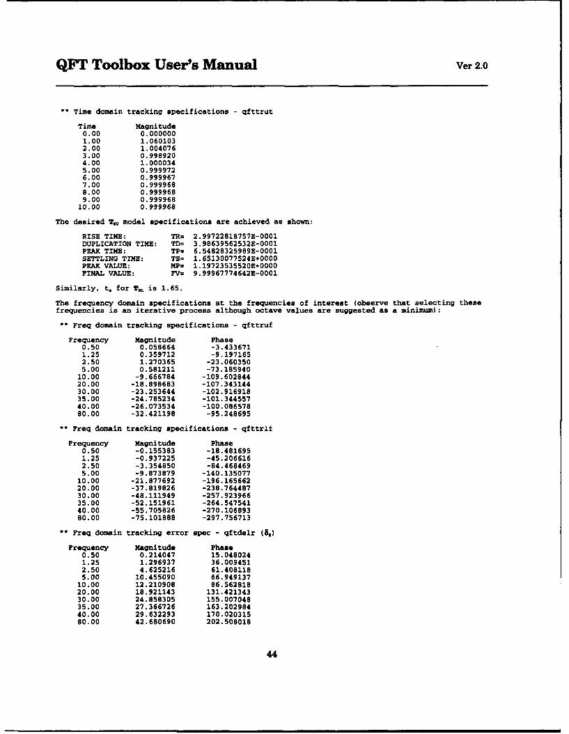
QFT Toolbox User's Manual Ver 2.0
** Time domain tracking specifications - qfttrut
Time Magnitude0.00 0.0000001.00 1.0601032.00 1.0040763.00 0.9989204.00 1.0000345.00 0.9999726.00 0.9999677.00 0.9999688.00 0.9999689.00 0.999968
10.00 0.999968
The desired Tu model specifications are achieved as shown:
RISE TIME: TR= 2.99722818757E-0001DUPLICATION TIME: TD= 3.98639562532E-0001PEAK TIME: TP= 6.54828325989E-0001SETTLING TIME: TS= 1.65130077524E+0000PEAK VALUE: MP= 1.19723535520E+0000FINAL VALUE: FV= 9.99967774642E-0001
Similarly, t. for TRL is 1.65.
The frequency domain specifications at the frequencies of interest (observe that selecting thesefrequencies is an iterative process although octave values are suggested as a minimum):
** Freq domain tracking specifications - qfttruf
Frequency Magnitude Phase0.50 0.058664 -3.4336711.25 0.359712 -9.1971652.50 1.270365 -23.0603505.00 0.581211 -73.185940
10.00 -9.666784 -109.60284420.00 -18.898683 -107.34314430.00 -23.253644 -102.91691835.00 -24.785234 -101.34455740.00 -26.073534 -100.08657880.00 -32.421198 -95.248695
** Freq domain tracking specifications - qfttrlf
Frequency Magnitude Phase0.50 -0.155383 -18.4816951.25 -0.937225 -45.2066162.50 -3.354850 -84.4684695.00 -9.873879 -140.135077
10.00 -21.877692 -196.16566220.00 -37.819826 -238.76448730.00 -48.111949 -257.92396635.00 -52.151961 -264.54754140.00 -55.705826 -270.10689380.00 -75.101888 -297.756713
** Freq domain tracking error spec - qftdelr (83)
Frequency Magnitude Phase0.50 0.214047 15.0480241.25 1.296937 36.0094512.50 4.625216 61.4081185.00 10.455090 66.949137
10.00 12.210908 86.56281820.00 18.921143 131.42134330.00 24.858305 155.00704835.00 27.366726 163.20298440.00 29.632293 170.02031580.00 42.680690 202.508018
44
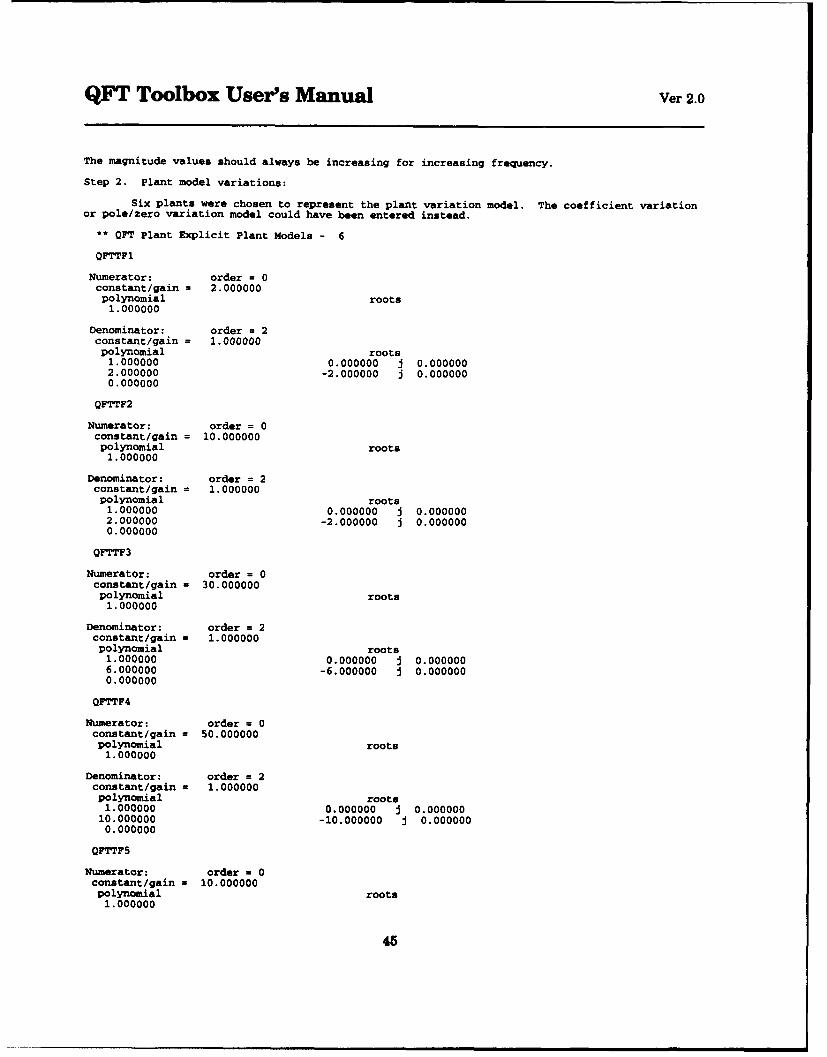
QFT Toolbox User's Manual Ver 2.0
The magnitude values should always be increasing for increasing frequency.
Step 2. Plant model variations:
Six plants were chosen to represent the plant variation model. The coefficient variationor pole/zero variation model could have been entered instead.
** QFT Plant Explicit Plant Models - 6
QFTTFl
Numerator: order = 0constant/gain = 2.000000polynomial roots
1.000000
Denominator: order = 2constant/gain = 1.000000polynomial roots
1.000000 0.000000 j 0.0000002.000000 -2.000000 j 0.0000000.000000
QFTTF2
Numerator: order = 0constant/gain = 10.000000polynomial roots
1.000000
Denominator: order = 2constant/gain = 1.000000polynomial roots
1.000000 0.000000 j 0.0000002.000000 -2.000000 j 0.0000000.000000
QFTTF3
Numerator: order = 0constant/gain = 30.000000polynomial roots
1.000000
Denominator: order = 2constant/gain = 1.000000polynomial roots
1.000000 0.000000 j 0.0000006.000000 -6.000000 j 0.0000000.000000
QFTTF4
Numerator: order = 0constant/gain = 50.000000polynomial roots
1.000000
Denominator: order = 2constant/gain = 1.000000polynomial roots
1.000000 0.000000 j 0.00000010.000000 -10.000000 j 0.0000000.000000
QFTTF5
Numerator: order a 0constant/gain = 10.000000polynomial roots
1.000000
45
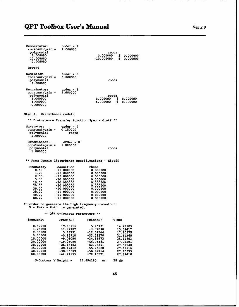
QFT Toolbox User's Manual Ver 2.0
Denominator: order = 2constant/gain = 1.000000polynomial roots
1.000000 0.000000 j 0.00000010.000000 -10.000000 j 0.0000000.000000
QFTTF6
Numerator: order = 0constant/gain = 6.000000polynomial roots
1.000000
Denominator: order = 2constant/gain = 1.000000polynomial roots
1.000000 0.000000 j 0.0000006.000000 -6.000000 j 0.0000000.000000
Step 3. Disturbance model:
** Disturbance Transfer Function Spec - distf *
Numerator: order = 0constant/gain = 0.100000polynomial roots
1.000000
Denominator: order = 0constant/gain = 1.000000polynomial roots
1.000000
** Freq domain disturbance specifications - distff
Frequency Magnitude Phase0.50 -20.000000 0.0000001.25 -20.000000 0.0000002.50 -20.000000 0.0000005.00 -20.000000 0.000000
10.00 -20.000000 0.00000020.00 -20.000000 0.00000030.00 -20.000000 0.00000035.00 -20.000000 0.00000040.00 -20.000000 0.00000080.00 -20.000000 0.000000
In order to generate the high frequency u-contour,
V = Pmax - Pmin is generated.
** QFT U-Contour Parameters *
frequency Pmax(dB) Pmin(dB) V(dB)
0.50000 19.98916 5.75731 14.231851.25000 11.97387 -3.37030 15.344172.50000 5.75731 -12.04544 17.802755.00000 -0.96910 -22.58278 21.61368
10.00000 -9.03090 -34.14973 25.1188320.00000 -19.03090 -46.06381 27.0329130.00000 -25.56303 -53.08351 27.5204835.00000 -28.12412 -55.75628 27.6321640.00000 -30.36629 -58.07264 27.7063580.00000 -42.21153 -70.10571 27.89418
U-Contour V Height = 27.894180 or 28 db
46
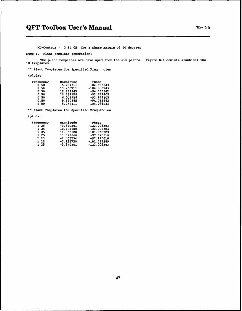
QFT Toolbox User's Manual Ver 2.0
ML-Contour = 3.84 dB for a phase margin of 40 degrees
Step 4. Plant template generation:
The plant templates are developed from the six plants. Figure B.1 depicts graphical the10 templates.
** Plant Templates for Specified Freqi-ncies
tpl.dat
Frequency Magnitude Phase0.50 5.757311 -104.0362430.50 19.736711 -104.0362430.50 19.969945 -94.7636420.50 19.989156 -92.8624050.50 6.009756 -92.8624050.50 5.990545 -94.7636420.50 5.757311 -104.036243
** Plant Templates for Specified Frequencies
tp2.dat
Frequency Magnitude Phase1.25 -3.370301 -122.0053831.25 10.609100 -122.0053831.25 11.856680 -101.7682891.25 11.973866 -97.1250161.25 -2.005534 -97.1250161.25 -2.122720 -101.7682891.25 -3.370301 -122.005383
47

QFT Toolbox User's Manual Ver 2.0
Fig B. 1
48
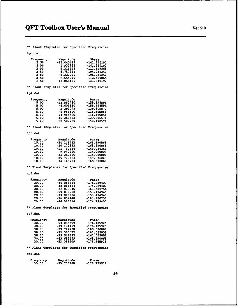
QFT Toolbox User's Manual Ver 2.0
** Plant Templates for Specified Frequencies
tp3.dat
Frequency Magnitude Phase2.50 -12.045439 -141.3401922.50 1.933961 -141.3401922.50 5.325358 -112.6198652.50 5.757311 -104.0362432.50 -8.222090 -104.0362432.50 -8.654042 -112.6198652.50 -12.045439 -141.340192
** Plant Templates for Specified Frequencies
tp4.dat
Frequency Magnitude Phase5.00 -22.582780 -158.1985915.00 -8.603380 -158.1985915.00 -2.290273 -129.8055715.00 -0.969100 -116.5650515.00 -14.948500 -116.5650515.00 -16.269673 -129.8055715.00 -22.582780 -158.198591
** Plant Templates for Specified Frequencies
tp5.dat
Frequency Magnitude Phase10.00 -34.149733 -168.69006810.00 -20.170333 -168.69006810.00 -11.792964 -149.03624310.00 -9.030900 -135.00000010.00 -23.010300 -135.00000010.00 -25.772364 -149.03624310.00 -34.149733 -168.690068
"* Plant Templates for Specified Frequencies
tp6.dat
Frequency Magnitude Phase20.00 -46.063814 -174.28940720.00 -32.084414 -174.28940720.00 -22.873040 -163.30075620.00 -19.030900 -153.43494920.00 -33.010300 -153.43494920.00 -36.852440 -163.30075620.00 -46.063814 -174.289407
** Plant Templates for Specified Frequencies
tp7.dat
Frequency Magnitude Phase30.00 -53.083509 -176.18592530.00 -39.104109 -176.18592530.00 -29.712758 -168.69006830.00 -25.563025 -161.56505130.00 -39.542425 -161.56505130.00 -43.692159 -168.69006830.00 -53.083509 -176.185925
"" Plant Templates for Specified Frequencies
tp8.dat
Frequency Magnitude Phase35.00 -55.756280 -176.729512
49
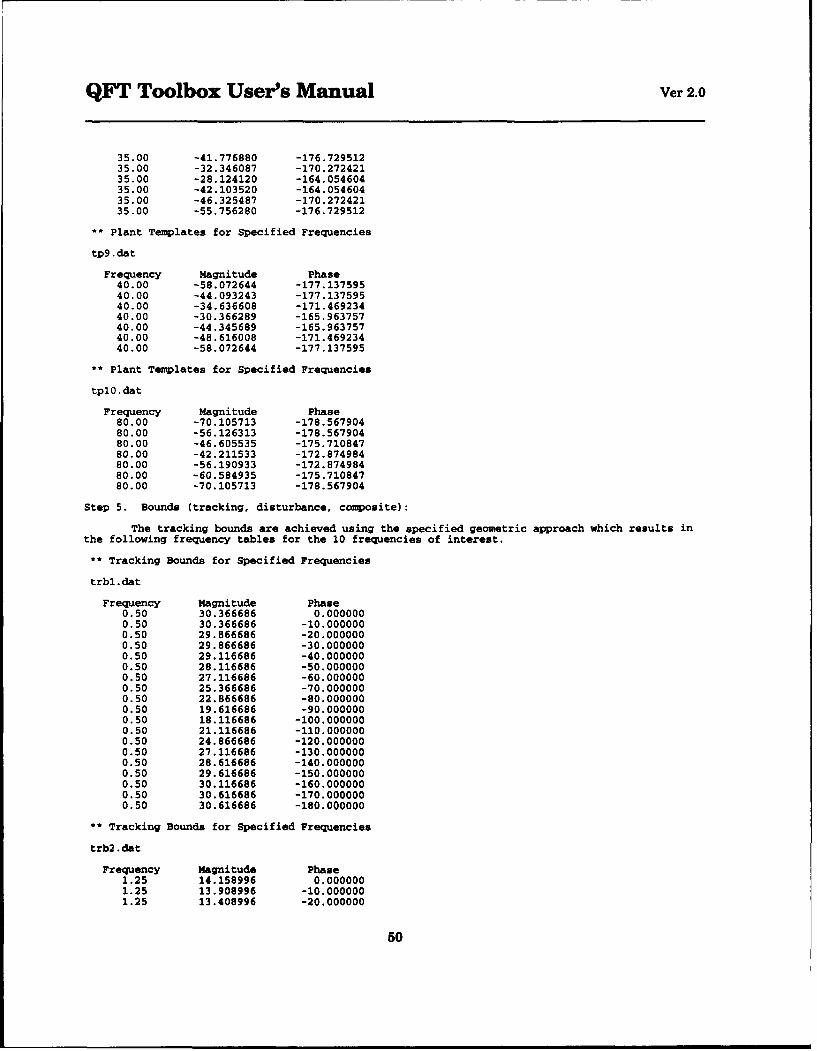
QFT Toolbox User's Manual Ver 2.0
35.00 -41.776880 -176.72951235.00 -32.346087 -170.27242135.00 -28.124120 -164.05460435.00 -42.103520 -164.05460435.00 -46.325487 -170.27242135.00 -55.756280 -176.729512
** Plant Templates for Specified Frequencies
tp9.dat
Frequency Magnitude Phase40.00 -58.072644 -177.13759540.00 -44.093243 -177.13759540.00 -34.636608 -171.46923440.00 -30.366289 -165.96375740.00 -44.345689 -165.96375740.00 -48.616008 -171.46923440.00 -58.072644 -177.137595
** Plant Templates for Specified Frequencies
tplO.dat
Frequency Magnitude Phase80.00 -70.105713 -178.56790480.00 -56.126313 -178.56790480.00 -46.605535 -175.71084780.00 -42.211533 -172.87498480.00 -56.190933 -172.87498480.00 -60.584935 -175.71084780.00 -70.105713 -178.567904
Step 5. Bounds (tracking, disturbance, composite):
The tracking bounds are achieved using the specified geometric approach which results inthe following frequency tables for the 10 frequencies of interest.
** Tracking Bounds for Specified Frequencies
trbl.dat
Frequency Magnitude Phase0.50 30.366686 0.0000000.50 30.366686 -10.0000000.50 29.866686 -20.0000000.50 29.866686 -30.0000000.50 29.116686 -40.0000000.50 28.116686 -50.0000000.50 27.116686 -60.0000000.50 25.366686 -70.0000000.50 22.866686 -80.0000000.50 19.616686 -90.0000000.50 18.116686 -100.0000000.50 21.116686 -110.0000000.50 24.866686 -120.0000000.50 27.116686 -130.0000000.50 28.616686 -140.0000000.50 29.616686 -150.0000000.50 30.116686 -160.0000000.50 30.616686 -170.0000000.50 30.616686 -180.000000
" Tracking Bounds for Specified Frequencies
trb2.dat
Frequency Magnitude Phase1.25 14.158996 0.0000001.25 13.908996 -10.0000001.25 13.408996 -20.000000
50
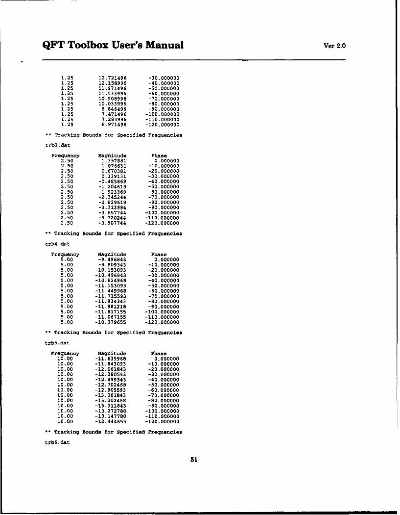
QFT Toolbox User's Manual Ver 2.0
1.25 12.721496 -30.0000001.25 12.158996 -40.0000001.25 11.971496 -50.0000001.25 11.533996 -60.0000001.25 10.908996 -70.0000001.25 10.033996 -80.0000001.25 8.846496 -90.0000001.25 7.471496 -100.0000001.25 7.283996 -110.0000001.25 8.971496 -120.000000
Tracking Bounds for Specified Frequencies
trb3.dat
Frequency Magnitude Phase2.50 1.357881 0.0000002.50 1.076631 -10.0000002.50 0.670381 -20.0000002.50 0.139131 -30.0000002.50 -0.485869 -40.0000002.50 -1.204619 -50.0000002.50 -1.923369 -60.0000002.50 -2.345244 -70.0000002.50 -2.829619 -80.0000002.50 -3.313994 -90.0000002.50 -3.657744 -100.0000002.50 -3.720244 -110.0000002.50 -3.907744 -120.000000
** Tracking Bounds for Specified Frequencies
trb4.dat
Frequency Magnitude Phase5.00 -9.496843 0.0000005.00 -9.809343 -10.0000005.00 -10.153093 -20.0000005.00 -10.496843 -30.0000005.00 -10.824968 -40.0000005.00 -11.153093 -50.0000005.00 -11.449968 -60.0000005.00 -11.715593 -70.0000005.00 -11.934343 -80.0000005.00 -11.981218 -90.0000005.00 -11.817155 -100.0000005.00 -11.067155 -110.0000005.00 -10.379655 -120.000000
** Tracking Bounds for Specified Frequencies
trb5.dat
Frequency Magnitude Phase10.00 -11.639968 0.00000010.00 -11.843093 -10.00000010.00 -12.061843 -20.00000010.00 -12.280593 -30.00000010.00 -12.499343 -40.00000010.00 -12.702468 -50.00000010.00 -12.905593 -60.00000010.00 -13.061843 -70.00000010.00 -13.202468 -80.00000010.00 -13.311843 -90.00000010.00 -13.272780 -100.00000010.00 -13.147780 -110.00000010.00 -12.444655 -120.000000
** Tracking Bounds for Specified Frequencies
trb6.dat
51

QFT Toolbox User's Manual Ver 2.0
Frequency Magnitude Phase20.00 -21.967134 0.00000020.00 -22.154634 -10.00000020.00 -22.264009 -20.00000020.00 -22.295259 -30.00000020.00 -22.248384 -40.00000020.00 -22.123384 -50.00000020.00 -21.920259 -60.00000020.00 -21.639009 -70.00000020.00 -21.310884 -80.00000020.00 -20.912446 -90.00000020.00 -20.474946 -100.00000020.00 -20.014009 -110.00000020.00 -19.326509 -120.000000
** Tracking Bounds for Specified Frequencies
trb7.dat
Frequency Magnitude Phase30.00 -35.676283 0.00000030.00 -35.863783 -10.00000030.00 -35.895033 -20.00000030.00 -35.707533 -30.00000030.00 -35.363783 -40.00000030.00 -34.801283 -50.00000030.00 -34.051283 -60.00000030.00 -33.082533 -70.00000030.00 -31.926283 -80.00000030.00 -30.582533 -90.00000030.00 -29.113783 -100.00000030.00 -27.582533 -110.00000030.00 -26.098158 -120.000000
** Tracking Bounds for Specified Frequencies
trb8.dat
Frequency Magnitude Phase35.00 -56.928155 0.00000035.00 -57.178155 -10.00000035.00 -57.178155 -20.00000035.00 -56.928155 -30.00000035.00 -56.178155 -40.00000035.00 -55.428155 -50.00000035.00 -54.178155 -60.00000035.00 -52.428155 -70.00000035.00 -49.928155 -80.00000035.00 -46.428155 -90.00000035.00 -41.303155 -100.00000035.00 -35.803155 -110.00000035.00 -31.365655 -120.000000
The disturbance bounds are achieved using the specified geometric approach which results
in the following frequency tables for the 10 frequencies of interest.
** Disturbance Bounds for Specified Frequencies
dbl.dat
Frequency Magnitude Phase0.50 4.841138 -10.0000000.50 4.866419 -20.0000000.50 4.932439 -30.0000000.50 5.022113 -40.0000000.50 5.132764 -50.0000000.50 5.261063 -60.0000000.50 5.403127 -70.0000000.50 5.554625 -80.0000000.50 5.710920 -90.000000
52
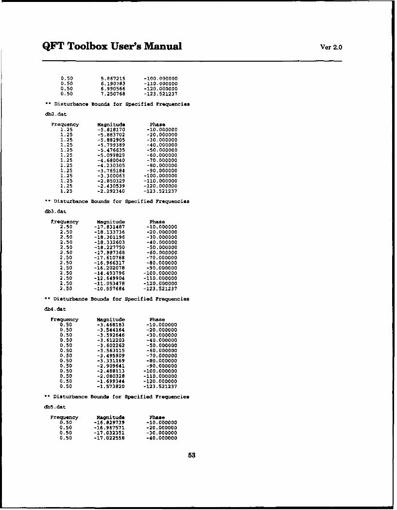
QFT Toolbox User's Manual Ver 2.0
0.50 5.867215 -100.0000000.50 6.190783 -110.0000000.50 6.990566 -120.0000000.50 7.250768 -123.521237
** Disturbance Bounds for Specified Frequencies
db2.dat
Frequency Magnitude Phase1.25 -5.818170 -10.0000001.25 -5.883702 -20.0000001.25 -5.882905 -30.0000001.25 -5.799389 -40.0000001.25 -5.476635 -50.0000001.25 -5.099829 -60.0000001.25 -4.680040 -70.0000001.25 -4.230305 -80.0000001.25 -3.765184 -90.0000001.25 -3.300063 -100.0000001.25 -2.850329 -110.0000001.25 -2.430539 -120.0000001.25 -2.292340 -123.521237
** Disturbance Bounds for Specified Frequencies
db3.dat
Itrequency Magnitude Phase2.50 -17.831487 -10.0000002.50 -18.133736 -20.0000002.50 -18.301196 -30.0000002.50 -18.332603 -40.0000002.50 -18.227750 -50.0000002.50 -17.987368 -60.0000002.50 -17.610768 -70.0000002.50 -16.966317 -80.0000002.50 -16.202078 -90.0000002.50 -14.493796 -100.0000002.50 -12.649904 -110.0000002.50 -11.053478 -120.0000002.50 -10.557684 -123.521237
** Disturbance Bounds for Specified Frequencies
db4.dat
Frequency Magnitude Phase0.50 -3.468183 -10.0000000.50 -3.544164 -20.0000000.50 -3.592646 -30.0000000.50 -3.612203 -40.0000000.50 -3.602262 -50.0000000.50 -3.563115 -60.0000000.50 -3.495909 -70.0000000.50 -3.331169 -80.0000000.50 -2.909641 -90.0000000.50 -2.488113 -100.0000000.50 -2.080328 -110.0000000.50 -1.699344 -120.0000000.50 -1.573820 -123.521237
** Disturbance Bounds for Specified Frequencies
db5.dat
Frequency Magnitude Phase0.50 -16.829739 -10.0000000.50 -16.967571 -20.0000000.50 -17.032351 -30.0000000.50 -17.022558 -40.000000
53
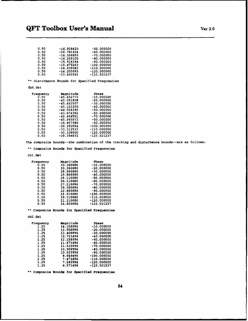
QFT Toolbox User's Manual Ver 2.0
0.50 -16.938420 -50.0000000.50 -16.781924 -60.0000000.50 -16.556893 -70.0000000.50 -16.269100 -80.0000000.50 -15.926364 -90.0000000.50 -15.475263 -100.0000000.50 -14.839083 -110.0000000.50 -14.203693 -120.0000000.50 -13.403941 -123.521237
** Disturbance Bounds for Specified Frequencies
db6.dat
Frequency Magnitude Phase0.50 -45.452773 -10.0000000.50 -45.591908 -20.0000000.50 -45.493507 -30.0000000.50 -45.153305 -40.0000000.50 -44.556190 -50.0000000.50 -43.674382 -60.0000000.50 -42.464581 -70.0000000.50 -40.865973 -80.0000000.50 -38.807586 -90.0000000.50 -36.252094 -100.0000000.50 -33.312533 -110.0000000.50 -30.336900 -120.0000000.50 -29.356833 -123.521237
The composite bounds--the combination of the tracking and disturbance bounds--are as follows:
** Composite Bounds for Specified Frequencies
cbl.dat
Frequency Magnitude Phase0.50 30.366686 -10.0000000.50 30.366686 -20.0000000.50 29.866686 -30.0000000.50 29.866686 -40.0000000.50 29.116686 -50.0000000.50 28.116686 -60.0000000.50 27.116686 -70.0000000.50 25.366686 -80.0000000.50 22.866686 -90.0000000.50 19.616686 -100.0000000.50 18.116686 -110.0000000.50 21.116686 -120.0000000.50 24.866686 -123.521237
** Composite Bounds for Specified Frequencies
cb2.dat
Frequency Magnitude Phase1.25 14.158996 -10.0000001.25 13.908996 -20.0000001.25 13.408996 -30.0000001.25 12.721496 -40.0000001.25 12.158996 -50.0000001.25 11.971496 -60.0000001.25 11.533996 -70.0000001.25 10.908996 -80.0000001.25 10.033996 -90.0000001.25 8.846496 -100.0000001.25 7.471496 -110.0000001.25 7.283996 -120.0000001.25 8.971496 -123.521237
** Composite Bounds for Specified Frequencies
54
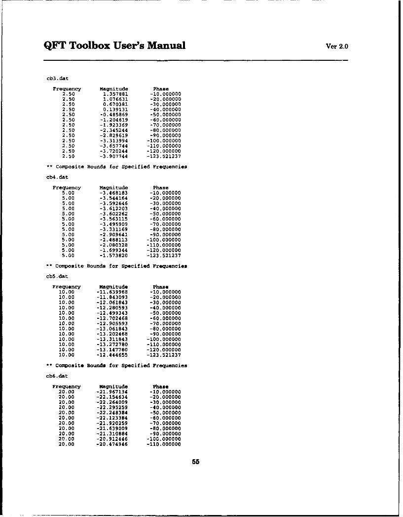
QFT Toolbox User's Manual Ver 2.0
cb3. da t
Frequency Magnitude Phase2.50 1.357881 -10.0000002.50 1.076631 -20.0000002.50 0.670381 -30.0000002.50 0.139131 -40.0000002.50 -0.485869 -50.0000002.50 -1.204619 -60.0000002.50 -1.923369 -70.0000002.50 -2.345244 -80.0000002.50 -2.829619 -90.0000002.50 -3.313994 -100.0000002.50 -3.657744 -110.0000002.50 -3.720244 -120.0000002.50 -3.907744 -123.521237
** Composite Bounds for Specified Frequencies
cb4.dat
Frequency Magnitude Phase5.00 -3.468183 -10.0000005.00 -3.544164 -20.0000005.00 -3.592646 -30.0000005.00 -3.612203 -40.0000005.00 -3.602262 -50.0000005.00 -3.563115 -60.0000005.00 -3.495909 -70.0000005.00 -3.331169 -80.0000005.00 -2.909641 -90.0000005.00 -2.488113 -100.0000005.00 -2.080328 -110.0000005.00 -1.699344 -120.0000005.00 -1.573820 -123.521237
** Composite Bounds for Specified Frequencies
cb5.dat
Frequency Magnitude Phase10.00 -11.639968 -10.00000010.00 -11.843093 -20.00000010.00 -12.061843 -30.00000010.00 -12.280593 -40.00000010.00 -12.499343 -50.00000010.00 -12.702468 -60.00000010.00 -12.905593 -70.00000010.00 -13.061843 -80.00000010.00 -13.202468 -90.00000010.00 -13.311843 -100.00000010.00 -13.272780 -110.00000010.00 -13.147780 -120.00000010.00 -12.444655 -123.521237
** Composite Bounds for Specified Frequencies
cb6.dat
Frequency Magnitude Phase20.00 -21.967134 -10.00000020.00 -22.154634 -20.00000020.00 -22.264009 -30.00000020.00 -22.295259 -40.00000020.00 -22.248384 -50.00000020.00 -22.123384 -60.00000020.00 -21.920259 -70.00000020.00 -21.639009 -80.00000020.00 -21.310884 -90.00000020.00 -20.912446 -100.00000020.00 -20.474946 -110.000000
55
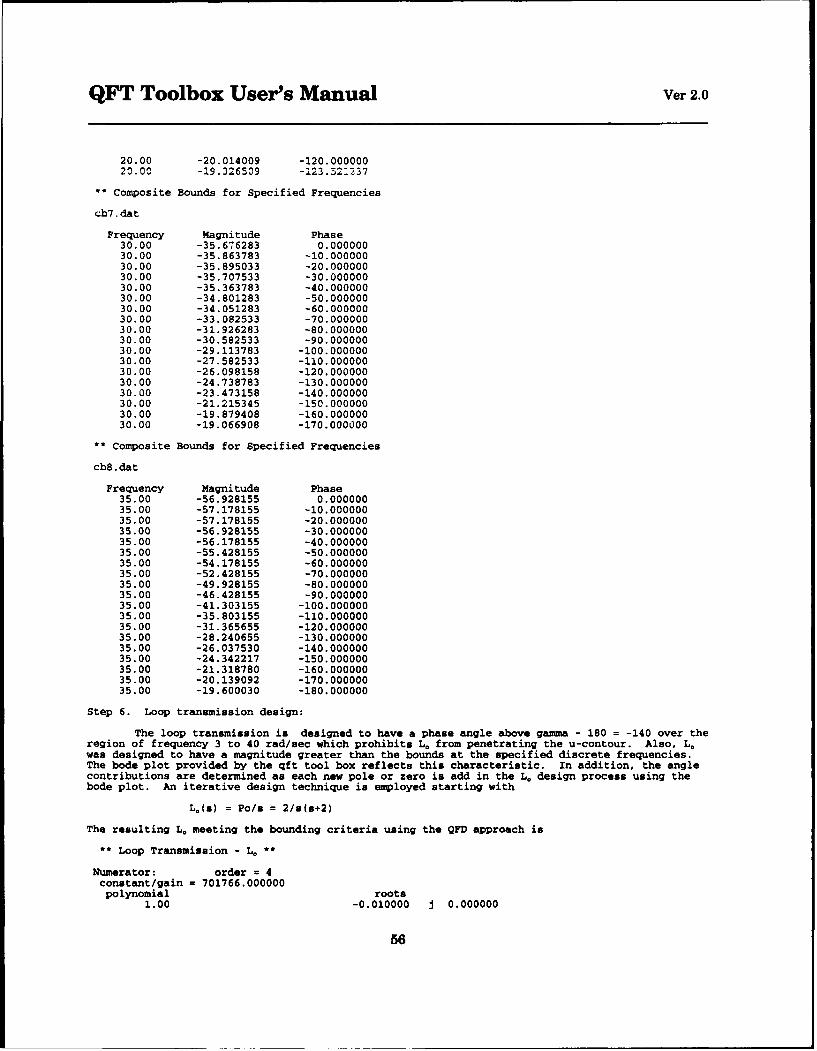
QFT Toolbox User's Manual Ver 2.0
20.00 -20.014009 -120.00000020.00 -19.326509 -123.52:237
** Composite Bounds for Specified Frequencies
cb7.dat
Frequency Magnitude Phase30.00 -35.676283 0.00000030.00 -35.863783 -10.00000030.00 -35.895033 -20.00000030.00 -35.707533 -30.00000030.00 -35.363783 -40.00000030.00 -34.801283 -50.00000030.00 -34.051283 -60.00000030.00 -33.082533 -70.00000030.00 -31.926283 -80.00000030.00 -30.582533 -90.00000030.00 -29.113783 -100.00000030.00 -27.582533 -110.00000030.00 -26.098158 -120.00000030.00 -24.738783 -130.00000030.00 -23.473158 -140.00000030.00 -21.215345 -150.00000030.00 -19.879408 -160.00000030.00 -19.066908 -170.000000
** Composite Bounds for Specified Frequencies
cb8.dat
Frequency Magnitude Phase35.00 -56.928155 0.00000035.00 -57.178155 -10.00000035.00 -57.178155 -20.00000035.00 -56.928155 -30.00000035.00 -56.178155 -40.00000035.00 -55.428155 -50.00000035.00 -54.178155 -60.00000035.00 -52.428155 -70.00000035.00 -49.928155 -80.00000035.00 -46.428155 -90.00000035.00 -41.303155 -100.00000035.00 -35.803155 -110.00000035.00 -31.365655 -120.00000035.00 -28.240655 -130.00000035.00 -26.037530 -140.00000035.00 -24.342217 -150.00000035.00 -21.318780 -160.00000035.00 -20.139092 -170.00000035.00 -19.600030 -180.000000
Step 6. Loop transmission design:
The loop transmission is designed to have a phase angle above ganma - 180 = -140 over theregion of frequency 3 to 40 rad/sec which prohibits L. from penetrating the u-contour. Also, L.was designed to have a magnitude greater than the bounds at the specified discrete frequencies.The bode plot provided by the qft tool box reflects this characteristic. In addition, the anglecontributions are determined as each new pole or zero is add in the L. design process using thebode plot. An iterative design technique is employed starting with
L0 (s) = Po/s = 2/s(s+2)
The resulting L. meeting the bounding criteria using the QFD approach is
** Loop Transmission - L. **
Numerator: order = 4constant/gain = 701766.000000polynomial roots
1.00 -0.010000 j 0.000000
56
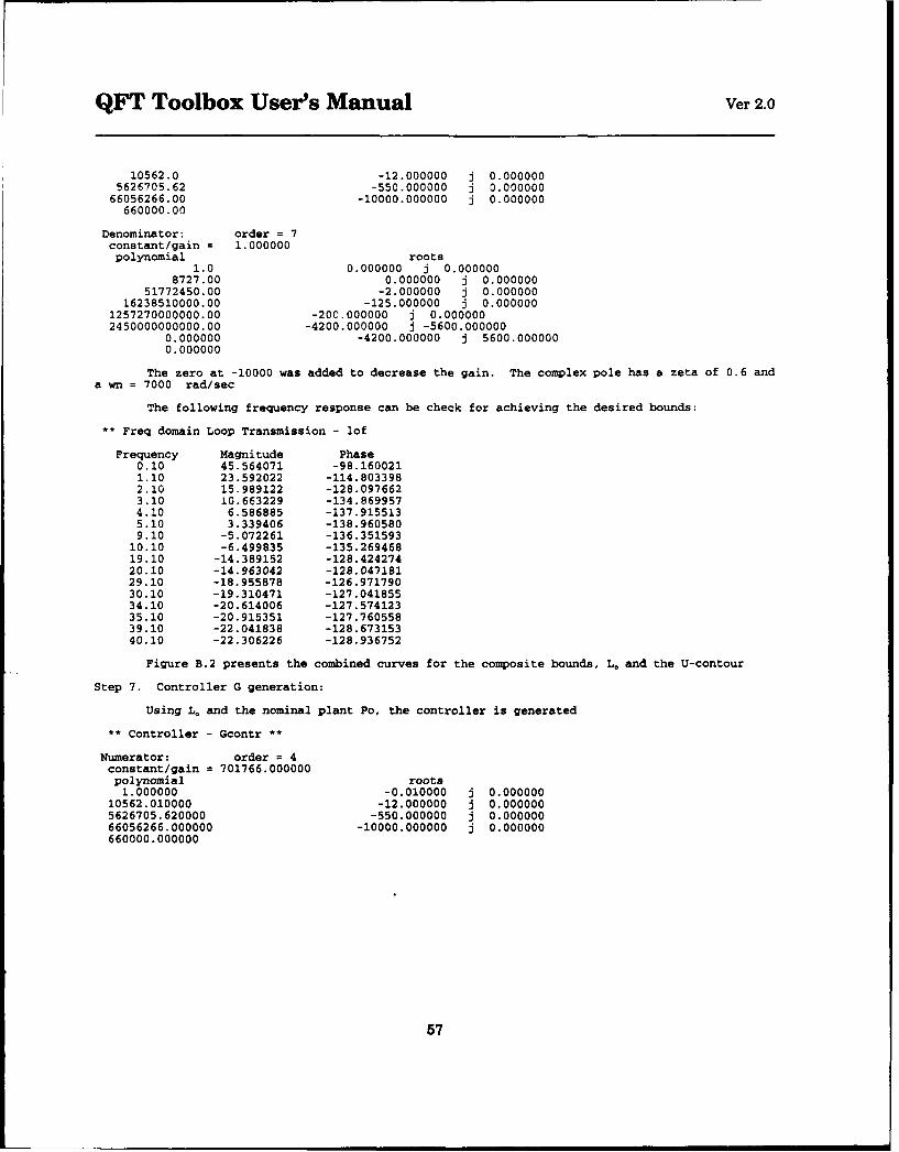
QFT Toolbox User's Manual Ver 2.0
10562.0 -12.000000 j 0.0000005626705.62 -550.000000 j 0.000000
66056266.00 -10000.000000 j 0.000000660000.00
Denominator: order = 7constant/gain f 1.000000polynomial roots
1.0 0.000000 j 0.0000008727.00 0.000000 j 0.000000
51772450.00 -2.000000 j 0.00000016238510000.00 -125.000000 j 0.000000
1257270000000.00 -20C.000000 j 0.0000002450000000000.00 -4200.000000 j -5600.000000
0.000000 -4200.000000 j 5600.0000000.000000
The zero at -10000 was added to decrease the gain. The complex pole has a zeta of 0.6 anda wn = 7000 rad/sec
The following frequency response can be check for achieving the desired bounds:
** Freq domain Loop Transmission - lof
Frequency Magnitude Phase0.10 45.564071 -98.1600211.10 23.592022 -114.8033982.10 15.989122 -128.0976623.10 10.663229 -134.8699574.10 6.586885 -137.9155135.10 3.339406 -138.9605809.10 -5.072261 -136.351593
10.10 -6.499835 -135.26946819.10 -14.389152 -128.42427420.10 -14.963042 -128.04718129.10 -18.955878 -126.97179030.10 -19.310471 -127.04185534.10 -20.614006 -127.57412335.10 -20.915351 -127.76055839.10 -22.041838 -128.67315340.10 -22.306226 -128.936752
Figure B.2 presents the combined curves for the composite bounds, L. and the U-contour
Step 7. Controller G generation:
Using L. and the nominal plant Po, the controller is generated
** Controller - Gcontr **
Numerator: order = 4constant/gain = 701766.000000polynomial roots
1.000000 -0.010000 j 0.00000010562.010000 -12.000000 j 0.0000005626705.620000 -550.000000 j 0.00000066056266.000000 -10000.000000 j 0.000000660000.000000
57
QFT Toolbox User's Manual Ver 2.0
Fig B.2
58
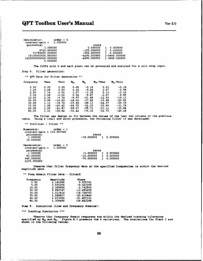
QFT Toolbox User's Manual Ver 2.0
Denominator: order = 5constant/gain = 2.000000polynomial roots
1.000000 0.000000 j 0.0000008725.000000 -125.000000 j 0.000000
51755000.000000 -200.000000 j 0.00000016135000000.000000 -4200.000000 j-5600.000000
1225000000000.000000 -4200.000000 j 5600.0000000.000000
The CLTFs with G and each plant can be generated and analyzed for a unit step input.
Step 8. Filter generation:
** QFT Data for Filter Generation **
frequency Tmax Tmin T1, TL TRu-Tmax TIL-Tmin
0.50 0.05 0.00 0.06 -0.16 0.01 -0.161.25 0.29 0.00 0.36 -0.94 0.07 -0.942.50 1.14 0.01 1.27 -3.35 0.13 -3.365.00 3.56 -0.02 0.58 -9.87 -2.97 -9.85
10.00 2.36 -3.74 -9.67 -21.88 -12.03 -18.1320.00 0.98 -14.00 -18.90 -37.82 -19.88 -23.8230.00 1.11 -18.72 -23.25 -48.11 -24.37 -29.3935.00 1.06 -20.42 -24.79 -52.15 -25.85 -31.7440.00 1.03 -21.87 -26.07 -55.71 -27.11 -33.8480.00 1.31 -29.82 -32.42 -75.10 -33.73 -45.28
The filter was design to fit between the values of the last two columns of the previoustable. Using a trail and error procedure, the following filter tf was developed:
"* Prefilter - filter **
Numerator: order = Iconstant/gain = 116.667000polynomial roots
1.000000 -18.000000 j 0.00000018.000000
Denominator: order = 3constant/gain = 1.000000polynomial roots
1.000000 -3.000000 j 0.00000083.000000 -10.000000 j 0.000000
940.000000 -70.000000 j 0.0000002100.000000
Observe that filter frequency data at the specified frequencies is within the desiredmagnitude band.
** Freq domain Filter Data - filterd
Frequency Magnitude Phase2.50 1.142266 0.0057015.00 3.555355 -0.023358
10.00 2.359959 -3.74395520.00 0.982747 -13.99525530.00 1.111816 -18.72476335.00 1.064837 -20.41644940.00 1.033052 -21.86713180.00 1.306490 -29.822368
Step 9. Simulation (time and frequency domains):
Tracking Simulation ***
Observe that frequency domain responses are within the desired tracking tolerancesspecified by Tm and T.. Figure B.3 presents the 6 variations. The simulations for Plant 1 areshown in the following tables:
59
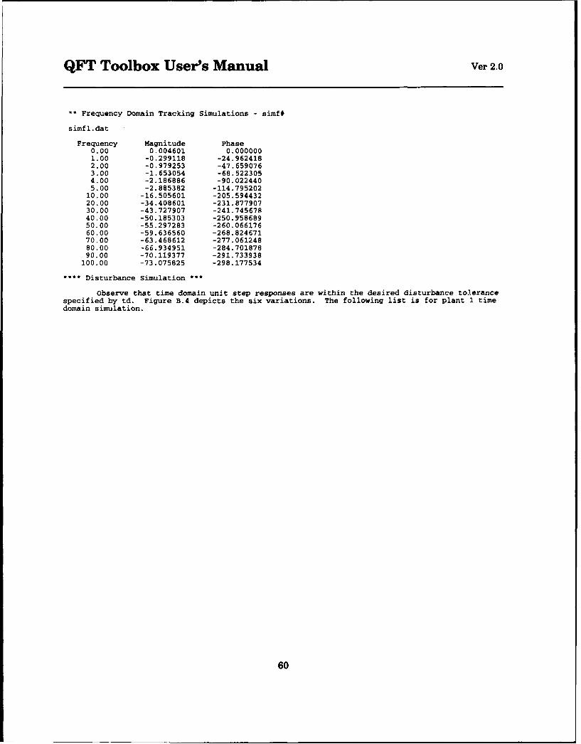
QFT Toolbox User's Manual Ver 2.0
** Frequency Domain Tracking Simulations - simf#
simfl.dat
Frequency Magnitude Phase0.00 0.004601 0.0000001.00 -0.299118 -24.9624182.00 -0.979253 -47.6590763.00 -1.653054 -68.5223054.00 -2.186886 -90.0224405.00 -2.885382 -114.795202
10.00 -16.505601 -205.59443220.00 -34.408601 -231.87790730.00 -43.727907 -241.74567840.00 -50.185303 -250.95868950.00 -55.297283 -260.06617660.00 -59.636560 -268.82467170.00 -63.468612 -277.06124880.00 -66.934951 -284.70187890.00 -70.119377 -291.733938
100.00 -73.075825 -298.177534
* Disturbance Simulation *
Observe that time domain unit step responses are within the desired disturbance tolerancespecified by td. Figure B.4 depicts the six variations. The following list is for plant 1 timedomain simulation.
60
QFT Toolbox User's Manual Ver 2.0
Fig B. 3
61
QFT Toolbox User's Manual Ver 2.0
Fig B.4
62
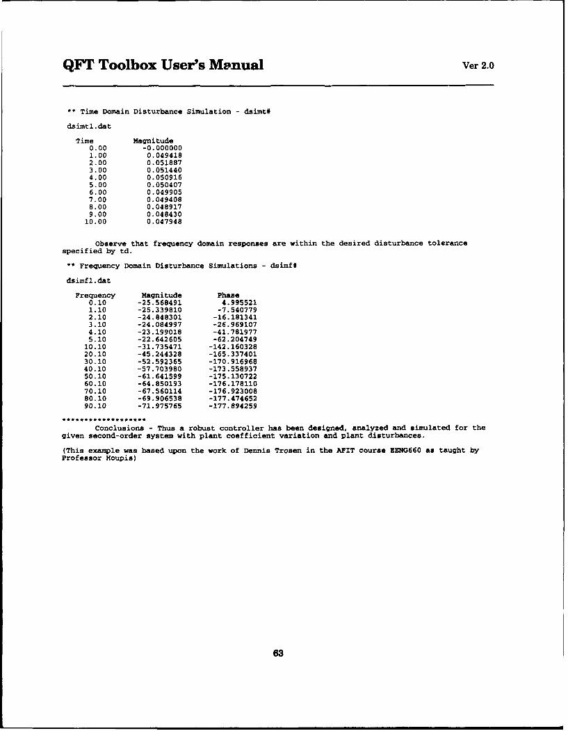
QFT Toolbox User's Menual Ver 2.0
** Time Domain Disturbance Simulation - dsimt#
dsimtl.dat
Time Magnitude0.00 -0.0000001.00 0.0494182.00 0.0518873.00 0.0514404.00 0.0509165.00 0.0504076.00 0.0499057.00 0.0494088.00 0.0489179.00 0.048430
10.00 0.047948
Observe that frequency domain responses are within the desired disturbance tolerance
specified by td.
** Frequency Domain Disturbance Simulations - dsimf#
dsimfl.dat
Frequency Magnitude Phase0.10 -25.568491 4.9955211.10 -25.339810 -7.5407792.10 -24.848301 -16.1813413.10 -24.084997 -26.9691074.10 -23.199018 -41.7819775.10 -22.642605 -62.204749
10.10 -31.735471 -142.16032820.10 -45.244328 -165.33740130.10 -52.592365 -170.91696840.10 -57.703980 -173.55893750.10 -61.641599 -175.13072260.10 -64.850193 -176.17811070.10 -67.560114 -176.92300880.10 -69.906538 -177.47465290.10 -71.975765 -177.894259
Conclusions - Thus a robust controller has been designed, analyzed and simulated for thegiven second-order system with plant coefficient variation and plant disturbances.
(This example was based upon the work of Dennis Trosen in the AFIT course EENG660 as taught byProfessor Houpis)
63

RFrf• T f D, OCU MENTAT!ON PAGE
.. .r•• TYPE AN) DAlft'i COV '
iDECEMBER 1992 Master's Thesis
777.77 5UNDi'd.. NU•MBERS
AN OBJECT-ORIENTED COMPUTER AIDED DESIGN PROGRAM FORTRADITIONAL CONTROL SYSTEMS ANALYSIS
Wayne E. Bell, ILT, USAF
-K1RT NJ,16ER
Air Force Institute of Technology, WPAFB OH 45433-5000
4CINCY N(. MEEP
AFIT/GE/ENG/92D-03
11 V\ *! A F: ý -, *AlfA FO Ij '21 F~~- k.N ý.C
Approved for public release; distribution unlimited
This thesis is a continuation of the ICECAP-PC research project conducted underProf. Gary B. Lamont at the Air Force Institute of Technology. It is an ongoingdevelopment of a public domain Computer Aided Design package for ControlEngineering and Digital Signal Processing students, faculty and practitionerswith a special emphasis on education. This investigation begins with thesoftware maintenance task of restructuring, debugging, and testing the functionalversion of ICECAP-PC 9.0. The continuous, traditional portions are then portedto a new object-oriented program structure which is the primary focus of thiseffort. New interactive graphics capabilities are then added as well as newprocedures for the time and frequency response plots. All basic math algorithmsare rewritten to be more accurate within a contemporary personal computerennvironment. Finally, using a program extension concept called a toolbox, aMultiple-Input-Single-Output (MISO) Quantitative Feedback Theory (OFT) toolbox iscreated. This toolbox allows manual, interactive, and automatic QFT design forcontinuous, linear, time invariant MISO control system problems.
1 ~1, NUI-BýR C,- PAGES
Computer Aided Control System Design (CACSD), Controls, 319Computer Aided Oesign(CAO),Quantitative Feedback Theory (OFT) 16 PqiE CODE
! (7177' t . ' (- , i y 7: ThON 19. SECURITY (IASSIF, ATIGN 2( ,'MTATIC'N Of ABSTRACT
Unclassified !Jd PHied UAnc OF ABSTRArs T U
Unclassified l#nclassi fied Unclassified UL