Ocean Emission Effects on Aerosol-Cloud Interactions: Insights from Two Case Studies

Hindawi Publishing CorporationAdvances in MeteorologyVolume 2010, Article ID 301395, 9 pagesdoi:10.1155/2010/301395

Research Article

Ocean Emission Effects on Aerosol-Cloud Interactions:Insights from Two Case Studies

Armin Sorooshian1, 2 and Hanh T. Duong1

1 Department of Chemical and Environmental Engineering, University of Arizona, P.O. Box 210011, Tucson, AZ 85721, USA2 Department of Atmospheric Sciences, University of Arizona, P.O. Box 210081, Tucson, AZ 85721, USA

Correspondence should be addressed to Armin Sorooshian, [email protected]

Received 9 January 2010; Revised 28 February 2010; Accepted 24 April 2010

Academic Editor: Markus D. Petters

Copyright © 2010 A. Sorooshian and H. T. Duong. This is an open access article distributed under the Creative CommonsAttribution License, which permits unrestricted use, distribution, and reproduction in any medium, provided the original work isproperly cited.

Two case studies are discussed that evaluate the effect of ocean emissions on aerosol-cloud interactions. A review of the first casestudy from the eastern Pacific Ocean shows that simultaneous aircraft and space-borne observations are valuable in detecting linksbetween ocean biota emissions and marine aerosols, but that the effect of the former on cloud microphysics is less clear owingto interference from background anthropogenic pollution and the difficulty with field experiments in obtaining a wide range ofaerosol conditions to robustly quantify ocean effects on aerosol-cloud interactions. To address these limitations, a second case wasinvestigated using remote sensing data over the less polluted Southern Ocean region. The results indicate that cloud drop size isreduced more for a fixed increase in aerosol particles during periods of higher ocean chlorophyll A. Potential biases in the resultsowing to statistical issues in the data analysis are discussed.

1. Introduction

Since oceans cover ∼70% of the earth surface, they representa massive source of gaseous and aerosol emissions thatmix with ship and continental emissions to form a highlycomplex soup of marine aerosol particles. Aerosols directlyinteract with solar radiation via scattering and absorption oflight, and they also serve as cloud condensation nuclei (CCN)and influence cloud properties and reflectivity. Attentionto the importance of aerosols in cloud and rain formationcan be traced back several decades ago to observations thatmaritime clouds exhibit lower droplet concentrations thansimilar clouds influenced by anthropogenic emissions overcontinental areas, and that the maritime clouds often rainin less than 30 minutes [1–3]. Since that time, researchhas pointed to two critical pieces of information linkingaerosols to warm clouds: (i) more numerous subcloudaerosol particles result in more reflective clouds (all elsebeing fixed) because of more abundant and smaller clouddroplets [4] and (ii) for more numerous and smaller clouddroplets, suppressed droplet collision-coalescence resultsin less precipitation [5]. But observational and modeling

studies often provide conflicting results with regard to themagnitude and even the sign of aerosol effects on clouds andprecipitation [6]. Furthermore, aerosol-cloud interactionsrepresent the largest uncertainty in assessments of the totalanthropogenic radiative forcing [7].

As shown in Figure 1 (see red arrows), aerosols areat the heart of the effect of ocean emissions on cloudproperties. The sources and nature of marine aerosols areinfluenced by some combination of ocean emissions, shipexhaust, and transported continental emissions. The task ofcharacterizing the optically and CCN-relevant properties ofmarine aerosols is overwhelming owing to the difficulty intheir measurement, their short atmospheric lifetime in themarine atmosphere, their spatial inhomogenieties, and thecomplexity of their composition. Just the organic fractionof aerosols alone is thought to comprise over thousands ofspecies that are virtually impossible to speciate altogether[8]. While it has long been known that ocean-emitteddimethylsulfide (DMS) plays a major role in influencing themarine CCN budget [9–11], recent studies have pointed tothe importance of other trace gas emissions such as isoprene[12–15] and organic amines [16, 17], which can partition

2 Advances in Meteorology

Aerosol

CCNactivation

Cloud microphysics

Precipitation

Wetscavenging

Meteorology

Radiativetransfer

Ocean

Ship exhaust +transported

continental emissions

Figure 1: Illustration of the interactive processes between oceans,aerosols, clouds, meteorology, and radiation in the marine atmo-sphere. The red arrows represent the sources of aerosols and thegreen and blue arrows collectively encompass the microphysicalprocesses associated with aerosol-cloud-precipitation interactions.

into the aerosol phase via secondary formation mechanisms[18–31]. Also, the importance of primary emissions of seaspray aerosols has long been recognized, but the significanceof primary biological aerosol particles is becoming moreevident as they have been shown to influence marineatmospheric processes more than previously assumed [32–41]. Although more will be learned about the physico-chemical properties of marine aerosols with advances ininstrumentation, a remaining uncertainty is the extent towhich various aerosol physicochemical properties affect thecloud microphysical and radiative response of clouds.

The effect of aerosols on clouds begins with the process ofcloud drop activation (Figure 1, green arrow). Observationaland modeling studies suggest that aside from dynamic effects(e.g., cloud base updraft velocity), the most importantaerosol physicochemical parameter governing cloud dropnumber concentration (Nd) is the aerosol size distribution[42–46], while aerosol composition is argued to be of sec-ondary importance [45]. However, under certain conditionsrelated to the degree of aerosol abundance or updraft velocitystrength, chemical effects have been shown to rival theaerosol size distribution with regard to the value of Nd

[47]. The current understanding of the drop activationprocess has benefited from both aerosol-CCN (e.g., [48–52]) and aerosol/CCN-Nd closure studies (e.g., [44, 53–55]).Although past closure studies have been met with limitedsuccess, one study in particular, that carried out an aerosol-Nd closure analysis using a cloud parcel model and aircraftmeasurements from a single platform [44], showed that Nd

within adiabatic cloud regions was within 15% (on average)of predictions. The accuracy of the drop activation processin models will continue to benefit from future studies of thisnature using improved experimental techniques.

In addition to drop activation, the overall microphysicalresponse of clouds (e.g., drop size) to aerosols is highlyuncertain owing to the difficulty in untangling aerosol effectson clouds in a buffered system [56]. Observational studiesface the challenging task of relating aerosol perturbationsto cloud microphysical responses (Figure 1, green and bluearrows) while removing meteorological effects. A failure toaccount for such meteorological factors, which refer to large-scale thermodynamic and dynamic parameters that dictatecloud properties on a larger scale, will yield misleadingresults. The introduction of state-of-the-art observationaltools such as NASA’s A-Train constellation of satellites[57] has provided valuable information related to aerosoland cloud properties with a high degree of spatial andtemporal coverage that cannot be obtained with dedicatedfield studies. Therefore, although there are many holes inthe current knowledge related to marine aerosols and theireffect on clouds and climate, new observational platformsare providing an unprecedented view of ocean-aerosol-cloudinteractions.

The goal of this work is twofold: (i) present two casestudies that examine ocean effects on aerosol-cloud inter-actions, specifically examining the steps leading from oceanemissions to a change in cloud drop size and (ii) discuss howresults from these case studies can improve future attemptsto quantify the links between oceans, aerosol particles, andclouds. Experimental methods used in this work are firstbriefly summarized. Then results are highlighted from arecent case study in the eastern Pacific Ocean region, wherethe drawbacks of that work are used to motivate a secondcase study in the Southern Ocean region that is subsequentlydescribed in detail.

2. Experimental Methods

Two case studies are presented below to explore oceaneffects on aerosol-cloud interactions. In both case studies,ocean chlorophyll A data are used from the Sea-viewingWide Field-of-view Sensor (Sea-WiFS; 8-day averaged data).Chlorophyll A is a proxy measurement of phytoplanktonbiomass and caution must be exercised when interpretingit as a proxy for primary production (i.e., biota emissions).The first case study focusing on the eastern Pacific Oceanregion (35.5◦ N–37◦ N, 122◦ W–123.5◦ W) is described indetail elsewhere [17], but is revisited here to highlightfindings that motivate the second case study. Briefly, aerosol,cloud, and meteorological measurements were carried outon-board the Center for Interdisciplinary Remotely-PilotedAircraft Studies (CIRPAS) Twin Otter as part of theMarine Stratus/Stratocumulus Experiment (MASE II) inJuly 2007. The relevant instrumentation ([17, see Table 1])included a forward scattering spectrometer probe (clouddrop distribution), a particle-into-liquid sampler (water-soluble composition) [58], a differential mobility analyzer(aerosol size distribution), and a continuous flow thermalgradient cloud condensation nuclei counter [59].

The second case study examines the spatial domain inthe Southern Ocean region encompassed by the following

Advances in Meteorology 3

Table 1: Summary of correlative relationships (r2) between ocean chlorophyll A, marine aerosols, and stratocumulus clouds during thethree-week MASE II field campaign in July 2007, during which chlorophyll A levels ranged between 1.01–3.58 mg m−3. Owing to the shortduration of the study and limited measurements of chlorophyll A (n = 3), all data have been averaged to correspond to the time durationscorresponding to each chlorophyll A measurement. Details related to the mean, standard deviation, and range of values of these parametersare discussed in detail by Sorooshian et al. [17]. (Chl A = chlorophyll A; DEA = diethylamine; MSA = methanesulfonate; Nd = cloud dropnumber concentration; TKE = turbulent kinetic energy).

Chl A DEA MSA Particle Conc. CCN (0.3%) Nd TKE

DEA 0.99

MSA 1.00 0.98

Particle Conc. 0.10 0.05 0.07

CCN (0.3%) 0.59 0.69 0.65 0.13

Nd 0.97 0.92 0.95 0.23 0.42

TKE 0.97 1.00 0.99 0.02 0.75 0.89

Wind speed 0.78 0.86 0.94 0.03 0.96 0.62 0.95

coordinates: 42◦ S–60◦ S, 180◦ W–180◦ E. Cloud and aerosolparameters are obtained from the Moderate ResolutionImaging Spectroradiometer (MODIS), specifically the 1◦

gridded aerosol index (Level 3, MODIS Collection 5) [60]and the drop effective radius (Level 2, 1-km resolution) [61].Aerosol index (AI) is taken as the product of the 0.55 μmaerosol optical depth × 0.55/0.867 μm Angstrom exponent,where the latter parameter accounts for the aerosol sizedistribution. MODIS is also used to derive cloud liquid waterpath (LWP; a product of the drop effective radius and cloudoptical depth). Lower tropospheric static stability (LTSS= potential temperature difference between 700 hPa and1000 hPa) estimates are derived from the European Centrefor Medium Range Weather Forecasts (ECMWF) analyses.This parameter serves as a proxy for the thermodynamic stateof the atmosphere [62]. A detailed screening procedure usingdata from the CloudSat cloud profiling radar, ECMWF-AUXiliary analysis (ECMWF-AUX), and MODIS is used toisolate only warm clouds for this case study analysis [63].

3. Case Study in the Eastern PacificOcean Region

A recent study off the coast of California pointed to theadvantage of simultaneously using multiple platforms ofanalysis to study ocean-aerosol-cloud interactions, while alsohighlighting experimental limitations to studying these inter-active processes in the coupled ocean-atmosphere system[17]. Table 1 presents a reanalysis of data from that study,specifically summarizing the degree of correlation betweenSea-WiFS-derived chlorophyll A, meteorological parameters,and aerosol and cloud properties. Biogenic tracers weredetected in the boundary layer aerosols during periodsof enhanced ocean emissions, including methanesulfonate(MSA, a dimethylsulfide oxidation product) and diethy-lamine (DEA). These two species were highly correlated withboth chlorophyll A and low-level wind speed (r2 > 0.86).Amines were shown to be a source of secondary organicaerosol in the marine atmosphere, which together with MSAaccounted for as high as 14% of the mass of sulfate duringthe peak chlorophyll A period. It is argued that rather than

predominantly being produced via new particle formationor being primarily emitted, that amines partitioned to theaerosol phase by condensation onto preexisting aerosols; thisis supported by the lack of a correlation between particleconcentration and either DEA/MSA/chlorophyll A (r2 ≤0.1), and with independent field [16, 64] and laboratorymeasurements [65] related to particulate amine production.

Subsaturated aerosol hygroscopic growth measurementsindicated that the organic component during periods of highchlorophyll A and wind speed exhibited considerable wateruptake ability. However, a critical limitation of the studywas the inability to distinguish between the effect of ocean-derived organics and other organics (e.g., ship emissions)on overall hygroscopicity. Enhanced CCN activity was alsoobserved, which was attributed to both size distribution andchemical effects, but again it was not possible to confidentlyattribute the change in CCN activity to the ocean-derivedorganics owing to the region of analysis.

Although in Table 1 it is shown that MSA/DEA/ chloro-phyll A are highly correlated with Nd (r2 ≥ 0.92), othermeteorological proxies such as turbulent kinetic energy (r2 =0.89) are also highly correlated with Nd. In order to quantifythe cloud microphysical response to an aerosol perturbation,it is necessary to account for meteorological conditions. Inother words, clouds with similar LWP (or some closely-related proxy) should be compared when determining howcloud droplet size varies with the subcloud aerosol concen-tration. Short-term field studies are faced with the challengeof obtaining a significant range of aerosol variability in binsof cloud LWP to afford a robust calculation of an aerosoleffect on cloud properties. For example, after removingdata clearly influenced by anthropogenic pollution (usingparticle concentration data and back-trajectory analysis) inthe current case study, only three events can be identifiedexhibiting a narrow range of meteorological conditions(turbulent kinetic energy was used as the meteorologicalproxy) to compare subcloud CCN to Nd (r2 = 0.41).Similarly, only three events were isolated with a narrow rangeof subcloud CCN concentration to correlate the turbulentkinetic energy to Nd (r2 = 0.95). Therefore, the limiteddataset indicates that meteorology influenced Nd to a greaterextent than aerosol effects, and that aerosol perturbations as


a result of higher chlorophyll A and wind speed may have hada secondary effect on Nd.

Two key limitations in this case study included the regionof analysis and the difficulty in obtaining a sufficiently widerange of aerosol conditions with surface- and aircraft-basedmeasurements to robustly quantify links between aerosolperturbations and cloud microphysical responses at fixedmeteorological conditions (i.e., LWP). The region off thecoast of California is characterized by a significant amountof background anthropogenic pollution, which makes itdifficult to identify a causal relationship between oceanemissions and cloud properties (i.e., change in drop size).Generally speaking, targeting links between ocean emissionsand aerosol and cloud properties may be difficult in manyregions of the globe where field studies are carried out owingto the significant amount of background pollution in theform of aged ship emissions and transported continentalemissions. A region that likely qualifies as a better ambientlaboratory to study the effects of marine biota emissionson cloud properties is the Southern Ocean, which is thefocus of the next case study that leverages satellite data.Limitations in data from dedicated field campaigns, as notedabove, strongly motivate the use of satellite data, which affordgreater temporal and spatial coverage (i.e., greater chance ofachieving a wide range of aerosol conditions as a function ofcloud regime).

4. Case Study in the Southern Ocean Region

This case study is motivated by previous work based onsatellite-based observations in the Southern Ocean region,which indicated that a link exists between phytoplanktonand cloudiness [13]. More specifically, cloud drop effectiveradius was shown to be reduced during periods of enhancedchlorophyll A, suggesting that enhanced phytoplanktonemissions lead to higher Nd. However, there is uncertaintyas to whether the inverse correlation between chlorophyll Aand drop effective radius is a robust relationship in differentglobal regions [17, 66].

The cloud microphysical response to aerosol pertur-bations is quantified in this analysis using the followingAerosol-Cloud Interaction metric [67]:

ACIr = −∂ ln re∂ lnα

(range = 0–0.33

), (1)

where re is the drop effective radius (at cloud top usingMODIS), α is a subcloud CCN proxy (AI in this analysis),and the partial derivative is evaluated with meteorologicalconditions held fixed (i.e., LWP). A higher value of ACIr canbe interpreted as meaning that for a fixed increase in AI,drop radius decreases more (all else fixed). The analysis isconducted for 11 LWP bins between 50 and 350 g m−2 andfor varying degrees of atmospheric stability, where data areseparated into conditions of relatively low stability (LTSS <15◦C) and high stability (LTSS > 18◦C). While the data arestratified into meteorological bins, it is noted that there stillis room for meteorological variability owing to measurementuncertainties and because the bins still exhibit a finite rangeof values. Satellite-derived ACIr values are reported only

0.8

0.7

0.6

0.5

0.4

0.3

0.2

0.1

Ch

loro

phyl

lA(m

gm−3

)

1/1/2000 1/1/2002 1/1/2004 1/1/2006 1/1/2008

UTC

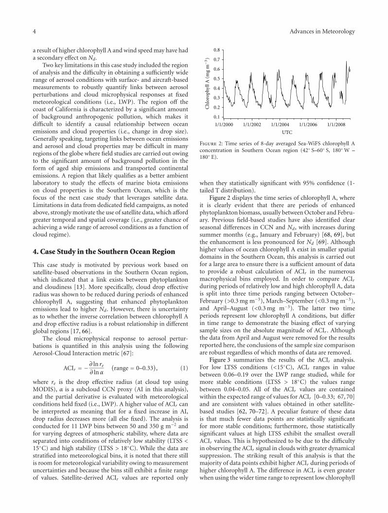
Figure 2: Time series of 8-day averaged Sea-WiFS chlorophyll Aconcentration in Southern Ocean region (42◦ S–60◦ S, 180◦ W –180◦ E).

when they statistically significant with 95% confidence (1-tailed T distribution).

Figure 2 displays the time series of chlorophyll A, whereit is clearly evident that there are periods of enhancedphytoplankton biomass, usually between October and Febru-ary. Previous field-based studies have also identified clearseasonal differences in CCN and Nd, with increases duringsummer months (e.g., January and February) [68, 69], butthe enhancement is less pronounced for Nd [69]. Althoughhigher values of ocean chlorophyll A exist in smaller spatialdomains in the Southern Ocean, this analysis is carried outfor a large area to ensure there is a sufficient amount of datato provide a robust calculation of ACIr in the numerousmacrophysical bins employed. In order to compare ACIrduring periods of relatively low and high chlorophyll A, datais split into three time periods ranging between October–February (>0.3 mg m−3), March–September (<0.3 mg m−3),and April–August (<0.3 mg m−3). The latter two timeperiods represent low chlorophyll A conditions, but differin time range to demonstrate the biasing effect of varyingsample sizes on the absolute magnitude of ACIr . Althoughthe data from April and August were removed for the resultsreported here, the conclusions of the sample size comparisonare robust regardless of which months of data are removed.

Figure 3 summarizes the results of the ACIr analysis.For low LTSS conditions (<15◦C), ACIr ranges in valuebetween 0.06–0.19 over the LWP range studied, while formore stable conditions (LTSS > 18◦C) the values rangebetween 0.04–0.05. All of the ACIr values are containedwithin the expected range of values for ACIr [0–0.33; 67, 70]and are consistent with values obtained in other satellite-based studies [62, 70–72]. A peculiar feature of these datais that much fewer data points are statistically significantfor more stable conditions; furthermore, those statisticallysignificant values at high LTSS exhibit the smallest overallACIr values. This is hypothesized to be due to the difficultyin observing the ACIr signal in clouds with greater dynamicalsuppression. The striking result of this analysis is that themajority of data points exhibit higher ACIr during periods ofhigher chlorophyll A. The difference in ACIr is even greaterwhen using the wider time range to represent low chlorophyll


Table 2: Statistical summary of the ACIr analysis shown in Figure 3. The numbers reported below represent ratios of a particular parameterbetween periods of relatively high chlorophyll A (>0.3 mg m−3; October–February) versus low chlorophyll A (<0.3 mg m−3; April–August).The average and standard deviation calculations are based on 11 values representing individual LWP bins between 50 and 350 g m−2. Theseresults represent 27 months of data starting in June 2006 for the Southern Ocean region (42◦ S–60◦ S, 180◦ W–180◦ E). (AI = aerosol index;AOD = aerosol optical depth; ANG = Angstrom exponent; re = cloud drop effective radius; min = minimum value; max = maximum value).

AI(min)

AI(max)

AI(range)

AOD(min)

AOD(max)

AOD(range)

ANG(min)

ANG(max)

ANG(range)

re(min)

re(max)

re(range)

Average 3.46 1.69 1.55 1.51 1.20 1.19 2.57 1.39 1.33 1.15 0.99 0.94

Std.Dev.

0.77 0.38 0.39 0.47 0.37 0.39 1.18 0.34 0.34 0.38 0.03 0.14

0.3

0.25

0.2

0.15

0.1

0.05

0

AC

I(C

hlA

>0.

3m

gm−3

)

0.30.250.20.150.10.050

ACI (Chl A < 0.3 mg m−3)

LTSS < 15 C, same sample size for high and low Chl ALTSS > 18 C, same sample size for high and low Chl A

LTSS < 15 C, 1.5–2 times as many points for low Chl A

Figure 3: Comparison of ACIr values (1) for periods of relativelyhigh and low chlorophyll A concentration in the Southern Oceanregion based on data over a span of 27 months starting in June 2006.Marker sizes are proportional to LWP between 50 and 350 g m−2 (11total LWP bins).

A conditions; this is presumably a result of larger samplesizes (greater by a factor of ∼1.5–2), and consequently adampening of the ACIr signal owing to a greater likelihoodof mixing different macrophysical conditions. To emphasizethat using a larger sample size at similar chlorophyll Aconditions will reduce the ACIr signal, ACIr is larger duringthe April–August time frame by a factor of 1.35 ± 0.28 ascompared to the March–September period.

When comparing comparable sample sizes for conditionsof high chlorophyll A and low chlorophyll A (April–August),the value of ACIr during the former period is greater bya factor of 1.3 ± 0.3. This result suggests that duringperiods of higher phytoplankton biomass a fixed increasein aerosol particles more strongly suppresses re because ofmore droplets for a fixed amount of cloud water. If this isthe case, a potential explanation for these results is that thosemarine aerosols during periods of higher chlorophyll A may

exhibit more favorable physicochemical properties (i.e., sizedistribution and chemical properties) with regard to dropletactivation. However, cautionary notes apply with regardto this conclusion owing to measurement and statisticaluncertainties. Table 2 highlights the issue of whether a “fair”statistical comparison was conducted during the identifiedperiods of high and low chlorophyll A conditions; it ishypothesized that a wider dynamic range in AI duringperiods of high chlorophyll A results in a more pronouncedACI signal using satellite data. Several ratios (minimum,maximum, range) are reported between periods of highversus low chlorophyll A for AI, AOD, Angstrom exponent,and re. It is shown that during periods of higher chlorophyllA, the minimum, maximum, and overall range of AI valueswas larger than those for low chlorophyll A conditions. Ofthe two AI subcomponents (AOD and Angstrom exponent),the range in the Angstrom exponent was larger (∼1.33) ascompared to AOD (1.19) during high chlorophyll A periodsversus low chlorophyll A periods. (It is noted that usingAOD as the subcloud CCN proxy in (1) results in an ACIrenhancement of 1.23 ± 0.66, which is slightly less than thatwhen using AI.) No enhancement was evident for cloud dropeffective radius (when analyzed in bins of cloud LWP), whichwas relatively similar for the two chlorophyll A conditions.Owing to the wider range of AI (and higher overall absolutevalues) during the period of enhanced chlorophyll A, it issuspected that the ACIr signal is more pronounced. Thelikely reason that the re values were more similar as comparedto AI (and its subcomponents) is that marine aerosolsare more closely linked physically to ocean emissions thanclouds (Figure 1). Therefore, although a link between higherchlorophyll A and enhanced AI values seems to be evident,the effect on cloud properties cannot be identified withhigh confidence using this dataset owing at least partly tostatistical factors in this analysis.

5. Conclusions

Two case studies were discussed that explore ocean effectson aerosol-cloud interactions in regions with different levelsof background anthropogenic pollution: off the Californiacoast and the Southern Ocean. The first study that isreviewed briefly in this work off the California coast [17]leveraged simultaneous satellite and field measurements toshow a direct link between ocean emissions and aerosol


physicochemical properties during periods of enhancedchlorophyll A and low-level wind speed, which otherwisewould not have been identified with any one measurementplatform alone. That work also pointed to the advantageof each individual platform of analysis (ground, airborne,satellite); for example, the aircraft measurements providedunique insight into the detailed aerosol physicochemicalproperties and their vertical atmospheric profiles. But adrawback with the aircraft and ground-based measurementswas the difficulty in obtaining a wide range of aerosolconditions at fixed meteorological conditions to robustlyquantify the cloud microphysical response to aerosol per-turbations during periods of varying ocean productivity.Furthermore, that region is characterized by a significantamount of background anthropogenic pollution, whichmade it challenging to isolate the effect of ocean biotaemissions on cloud properties.

Owing to the ambiguity of the results related to oceanemissions on aerosol-cloud interactions in the first casestudy, a second investigation was carried out for the SouthernOcean region owing to its lower amount of backgroundanthropogenic pollution. In order to examine aerosol effectson clouds in this area during periods of relatively low andhigh chlorophyll A conditions, ACIr (1) was quantified whileaccounting for macrophysical factors such as atmosphericstability and cloud LWP. The cloud microphysical responseto aerosol perturbations was stronger (higher ACIr) duringperiods of higher chlorophyll A. This indicates that clouddrop size experiences a greater reduction for a fixed increasein aerosol concentration, potentially as a result of aerosolswith more favorable physicochemical properties for dropletactivation. But a causal relationship is difficult to establishowing to biasing factors in the datasets. It is shown thatduring periods of higher chlorophyll A, the range andminimum/maximum values of AI and its subcomponents(AOD and Angstrom exponent) are higher than thoseduring low-chlorophyll A periods. Although this points tohigher aerosol concentrations during times characterized byenhanced phytoplankton biomass, it also suggests that theACIr signal may be more pronounced owing to the widerrange in AI. It is argued that this does not allow for a“fair” comparison and it points to the need to considersuch issues in future studies. Another factor shown to biasACIr values is sample size, where an increase in the amountof data led to a reduction in ACIr for conditions of lowchlorophyll A presumably owing to a greater likelihood ofmixing data across a wider range of meteorological and cloudconditions.

The topic of ocean-aerosol-cloud interactions will benefitfrom future analyses with more extensive datasets at higherspatial resolution. Field measurements are needed in addi-tion to satellite observations to quantify the physicochemicalproperties of marine aerosols (e.g., size and composition)and to probe more detailed issues such as the role ofsurface-active and directly-emitted aerosol particles [73–78]in influencing Nd and cloud albedo. In addition, comple-mentary modeling-based studies (e.g., [79–84]), are essentialin advancing predictions of marine aerosol emissions andtheir impacts on clouds and climate.

Acknowledgments

We acknowledge support from Office of Naval Researchgrant N00014-10-1-0811. The authors acknowledge MattLebsock for assistance with satellite data. Ocean chlorophyllA data used in this study were acquired using the GES-DISCInteractive Online Visualization ANd aNalysis Infrastructure(Giovanni) as part of the NASA’s Goddard Earth Sciences(GES) Data and Information Services Center (DISC).

References

[1] P. Squires, “The microstructure of cumuli in maritime andcontinental air,” Tellus, vol. 8, pp. 443–444, 1956.

[2] P. Squires, “Penetrative downdraughts in cumuli,” Tellus, vol.10, pp. 381–389, 1958.

[3] P. Squires and S. Twomey, “A comparison of cloud nucleusmeasurements over central north america and caribbean sea,”Journal of the Atmospheric Sciences, vol. 23, pp. 401–404, 1966.

[4] S. Twomey, “Influence of pollution on shortwave albedo ofclouds,” Journal of the Atmospheric Sciences, vol. 34, pp. 1149–1152, 1977.

[5] B. A. Albrecht, “Aerosols, cloud microphysics, and fractionalcloudiness,” Science, vol. 245, no. 4923, pp. 1227–1230, 1989.

[6] A. P. Khain, “Notes on state-of-the-art investigations ofaerosol effects on precipitation: a critical review,” Environmen-tal Research Letters, vol. 4, no. 1, Article ID 015004, 2009.

[7] IPCC, “Summary for policymakers,” in Climate Change 2007:The Physical Science Basis. Contribution of Working Group I tothe Fourth Assessment Report of the Intergovernmental Panel onClimate Change, S. Solomon, D. Qin, M. Manning, et al., Eds.,Cambridge University Press, New York, NY, USA, 2007.

[8] A. H. Goldstein and I. E. Galbally, “Known and unexploredorganic constituents in the earth’s atmosphere,” EnvironmentalScience and Technology, vol. 41, no. 5, pp. 1514–1521, 2007.

[9] M. O. Andreae and H. Raemdonck, “Dimethyl sulfide in thesurface ocean and the marine atmosphere: a global view,”Science, vol. 221, no. 4612, pp. 744–747, 1983.

[10] G. E. Shaw, “Bio-controlled thermostasis involving the sulfurcycle,” Climatic Change, vol. 5, no. 3, pp. 297–303, 1983.

[11] R. J. Charlson, J. E. Lovelock, M. O. Andreae, and S. G. Warren,“Oceanic phytoplankton, atmospheric sulphur, cloud albedoand climate,” Nature, vol. 326, no. 6114, pp. 655–661, 1987.

[12] M. Claeys, B. Graham, G. Vas et al., “Formation of secondaryorganic aerosols through photooxidation of isoprene,” Science,vol. 303, no. 5661, pp. 1173–1176, 2004.

[13] N. Meskhidze and A. Nenes, “Phytoplankton and cloudinessin the southern ocean,” Science, vol. 314, no. 5804, pp. 1419–1423, 2006.

[14] S. R. Arnold, D. V. Spracklen, J. Williams et al., “Evaluation ofthe global oceanic isoprene source and its impacts on marineorganic carbon aerosol,” Atmospheric Chemistry and Physics,vol. 9, no. 4, pp. 1253–1262, 2009.

[15] S. Ekstrom, B. Noziere, and H.-C. Hansson, “The cloudcondensation nuclei (CCN) properties of 2-methyltetrols andC3-C6 polyols from osmolality and surface tension measure-ments,” Atmospheric Chemistry and Physics, vol. 9, no. 3, pp.973–980, 2009.

[16] M. C. Facchini, S. Decesari, M. Rinaldi et al., “Importantsource of marine secondary organic aerosol from biogenicamines,” Environmental Science and Technology, vol. 42, no. 24,pp. 9116–9121, 2008.


[17] A. Sorooshian, L. T. Padro, A. Nenes, et al., “On the linkbetween ocean biota emissions, aerosol, and maritime clouds:airborne, ground, and satellite measurements off the coast ofCalifornia,” Global Biogeochemical Cycles, vol. 23, no. 4, ArticleID GB4007, p. 15, 2009.

[18] C. D. O’Dowd and G. de Leeuw, “Marine aerosol production:a review of the current knowledge,” Philosophical Transactionsof the Royal Society A, vol. 365, no. 1856, pp. 1753–1774, 2007.

[19] J. Liggio, S.-M. Li, and R. McLaren, “Heterogeneous reactionsof glyoxal on particulate matter: identification of acetals andsulfate esters,” Environmental Science and Technology, vol. 39,no. 6, pp. 1532–1541, 2005.

[20] R. Volkamer, P. J. Ziemann, and M. J. Molina, “Secondaryorganic aerosol formation from acetylene (C2H 2): seed effecton SOA yields due to organic photochemistry in the aerosolaqueous phase,” Atmospheric Chemistry and Physics, vol. 9, no.4, pp. 1907–19028, 2009.

[21] A. L. Corrigan, S. W. Hanley, and D. O. De Haan, “Uptakeof glyoxal by organic and inorganic aerosol,” EnvironmentalScience and Technology, vol. 42, no. 12, pp. 4428–4433, 2008.

[22] C. J. Hennigan, M. H. Bergin, J. E. Dibb, and R. J. Weber,“Enhanced secondary organic aerosol formation due to wateruptake by fine particles,” Geophysical Research Letters, vol. 35,no. 18, Article ID L18801, 5 pages, 2008.

[23] J. D. Blando and B. J. Turpin, “Secondary organic aerosolformation in cloud and fog droplets: a literature evaluationof plausibility,” Atmospheric Environment, vol. 34, no. 10, pp.1623–1632, 2000.

[24] P. Warneck, “In-cloud chemistry opens pathway to the for-mation of oxalic acid in the marine atmosphere,” AtmosphericEnvironment, vol. 37, no. 17, pp. 2423–2427, 2003.

[25] K. K. Crahan, D. Hegg, D. S. Covert, and H. Jonsson, “Anexploration of aqueous oxalic acid production in the coastalmarine atmosphere,” Atmospheric Environment, vol. 38, no. 23,pp. 3757–3764, 2004.

[26] B. Ervens, G. Feingold, G. J. Frost, and S. M. Kreidenweis,“A modeling of study of aqueous production of dicarboxylicacids: 1. Chemical pathways and speciated organic massproduction,” Journal of Geophysical Research, vol. 109, no. 15,Article ID D15205, 20 pages, 2004.

[27] J. Z. Yu, X.-F. Huang, J. Xu, and M. Hu, “When aerosol sulfategoes up, so does oxalate: implication for the formation mech-anisms of oxalate,” Environmental Science and Technology, vol.39, no. 1, pp. 128–133, 2005.

[28] A. Sorooshian, V. Varutbangkul, F. J. Brechtel et al., “Oxalicacid in clear and cloudy atmospheres: analysis of datafrom international consortium for atmospheric research ontransport and transformation 2004,” Journal of GeophysicalResearch, vol. 111, no. 23, Article ID D23S45, 17 pages, 2006.

[29] A. Sorooshian, M.-L. Lu, F. J. Brechtel et al., “On the sourceof organic acid aerosol layers above clouds,” EnvironmentalScience and Technology, vol. 41, no. 13, pp. 4647–4654, 2007.

[30] A. G. Carlton, B. J. Turpin, K. E. Altieri et al., “Atmosphericoxalic acid and SOA production from glyoxal: results of aque-ous photooxidation experiments,” Atmospheric Environment,vol. 41, no. 35, pp. 7588–7602, 2007.

[31] K. E. Altieri, S. P. Seitzinger, A. G. Carlton, B. J. Turpin, G.C. Klein, and A. G. Marshall, “Oligomers formed through in-cloud methylglyoxal reactions: chemical composition, proper-ties, and mechanisms investigated by ultra-high resolution FT-ICR mass spectrometry,” Atmospheric Environment, vol. 42,no. 7, pp. 1476–1490, 2008.

[32] M. L. Wells and E. D. Goldberg, “Occurrence of small colloidsin sea water,” Nature, vol. 353, no. 6342, pp. 342–344, 1991.

[33] M. L. Wells and E. D. Goldberg, “Colloid aggregation inseawater,” Marine Chemistry, vol. 41, no. 4, pp. 353–358, 1993.

[34] R. Benner, J. D. Pakulski, M. McCarthy, J. I. Hedges, and P. G.Hatcher, “Bulk chemical characteristics of dissolved organicmatter in the ocean,” Science, vol. 255, no. 5051, pp. 1561–1564, 1992.

[35] M. L. Wells, “Marine colloids—a neglected dimension,”Nature, vol. 391, no. 6667, pp. 530–531, 1998.

[36] E. K. Bigg, C. Leck, and L. Tranvik, “Particulates of thesurface microlayer of open water in the central Arctic Oceanin summer,” Marine Chemistry, vol. 91, no. 1–4, pp. 131–141,2004.

[37] C. Leck and E. K. Bigg, “Biogenic particles in the surfacemicrolayer and overlaying atmosphere in the central ArcticOcean during summer,” Tellus, Series B, vol. 57, no. 4, pp. 305–316, 2005.

[38] C. Leck and E. K. Bigg, “Source and evolution of the marineaerosol—a new perspective,” Geophysical Research Letters, vol.32, no. 19, Article ID L19803, 4 pages, 2005.

[39] R. Jaenicke, “Abundance of cellular material and proteins inthe atmosphere,” Science, vol. 308, no. 5718, 73 pages, 2005.

[40] E. K. Bigg, “Sources, nature and influence on climate of marineairborne particles,” Environmental Chemistry, vol. 4, no. 3, pp.155–161, 2007.

[41] V. R. Despres, J. F. Nowoisky, M. Klose, R. Conrad, M.O. Andreae, and U. Poschl, “Characterization of primarybiogenic aerosol particles in urban, rural, and high-alpineair by DNA sequence and restriction fragment analysis ofribosomal RNA genes,” Biogeosciences, vol. 4, no. 6, pp. 1127–1141, 2007.

[42] J. W. Fitzgerald, “Effect of aerosol composition on clouddroplet size distribution—numerical study,” Journal of theAtmospheric Sciences, vol. 31, pp. 1358–1367, 1974.

[43] G. Feingold, “Modeling of the first indirect effect: analysis ofmeasurement requirements,” Geophysical Research Letters, vol.30, no. 19, pp. 7–4, 2003.

[44] W. C. Conant, T. M. VanReken, T. A. Rissman et al., “Aerosol-cloud drop concentration closure in warm cumulus,” Journalof Geophysical Research, vol. 109, no. 13, Article ID D13204, 12pages, 2004.

[45] B. Ervens, G. Feingold, and S. M. Kreidenweis, “Influenceof water-soluble organic carbon on cloud drop numberconcentration,” Journal of Geophysical Research, vol. 110, no.18, Article ID D18211, 14 pages, 2005.

[46] U. Dusek, G. P. Frank, L. Hildebrandt et al., “Size mattersmore than chemistry for cloud-nucleating ability of aerosolparticles,” Science, vol. 312, no. 5778, pp. 1375–1378, 2006.

[47] A. Nenes, R. J. Charlson, M. C. Facchini, M. Kulmala, A.Laaksonen, and J. H. Seinfeld, “Can chemical effects on clouddroplet number rival the first indirect effect?” GeophysicalResearch Letters, vol. 29, no. 17, article 1848, 4 pages, 2002.

[48] T. M. VanReken, T. A. Rissman, G. C. Roberts et al., “Towardaerosol/cloud condensation nuclei (CCN) closure duringCRYSTAL-FACE,” Journal of Geophysical Research, vol. 108, no.D20, article 4633, 18 pages, 2003.

[49] P. S. K. Liu, W. R. Leaitch, C. M. Banic, S.-M. Li, D. Ngo, andW. J. Megaw, “Aerosol observations at chebogue point duringthe 1993 North Atlantic regional experiment: relationshipsamong cloud condensation nuclei, size distribution, andchemistry,” Journal of Geophysical Research, vol. 101, no. 22,pp. 28971–28990, 1996.


[50] D. S. Covert, J. L. Gras, A. Wiedensohler, and F. Stratmann,“Comparison of directly measured CCN with CCN modeledfrom the number-size distribution in the marine boundarylayer during ACE 1 at Cape Grim, Tasmania,” Journal ofGeophysical Research, vol. 103, no. 13, pp. 16597–16608, 1998.

[51] W. Cantrell, G. Shaw, G. R. Cass et al., “Closure betweenaerosol particles and cloud condensation nuclei at kaashidhooclimate observatory,” Journal of Geophysical Research, vol. 106,no. 22, pp. 28711–28718, 2001.

[52] J. R. Snider, S. Guibert, J.-L. Brenguier, and J.-P. Putaud,“Aerosol activation in marine stratocumulus clouds: 2. Kohlerand parcel theory closure studies,” Journal of GeophysicalResearch, vol. 108, no. 15, article 8629, 23 pages, 2003.

[53] S. Twomey and J. Warner, “Comparison of measurements ofcloud droplets and cloud nuclei,” Journal of the AtmosphericSciences, vol. 24, pp. 702–703, 1967.

[54] J. W. Fitzgerald and P. Spyers-Duran, “Changes in cloudnucleus concentration and cloud droplet size distributionassociated with pollution from St. Louis,” Journal of AppliedMeteorology, vol. 30, pp. 511–516, 1973.

[55] J. R. Snider and J.-L. Brenguier, “Cloud condensation nucleiand cloud droplet measurements during ACE-2,” Tellus, SeriesB, vol. 52, no. 2, pp. 828–842, 2000.

[56] B. Stevens and G. Feingold, “Untangling aerosol effects onclouds and precipitation in a buffered system,” Nature, vol.461, no. 7264, pp. 607–613, 2009.

[57] G. L. Stephens, D. G. Vane, R. J. Boain et al., “The cloudsatmission and the a-train: a new dimension of space-basedobservations of clouds and precipitation,” Bulletin of theAmerican Meteorological Society, vol. 83, no. 12, pp. 1771–1742, 2002.

[58] A. Sorooshian, F. J. Brechtel, Y. L. Ma, et al., “Modelingand characterization of a particle-into-liquid sampler (PILS),”Aerosol Science and Technology, vol. 40, pp. 396–409, 2006.

[59] G. C. Roberts and A. Nenes, “A continuous-flow streamwisethermal-gradient CCN chamber for atmospheric measure-ments,” Aerosol Science and Technology, vol. 39, no. 3, pp. 206–221, 2005.

[60] L. A. Remer, Y. J. Kaufman, D. Tanre et al., “The MODISaerosol algorithm, products, and validation,” Journal of theAtmospheric Sciences, vol. 62, no. 4, pp. 947–973, 2005.

[61] S. Platnick, M. D. King, S. A. Ackerman et al., “The MODIScloud products: algorithms and examples from terra,” IEEETransactions on Geoscience and Remote Sensing, vol. 41, no. 2,pp. 459–473, 2003.

[62] S. A. Klein and D. L. Hartmann, “The seasonal cycle of lowstratiform clouds,” Journal of Climate, vol. 6, no. 8, pp. 1587–1606, 1993.

[63] M. D. Lebsock, G. L. Stephens, and C. Kummerow, “Theseasonal cycle of low stratiform clouds,” Journal of GeophysicalResearch, vol. 113, no. 8, Article ID D15205, 12 pages, 2008.

[64] A. Sorooshian, S. M. Murphy, S. Hersey et al., “Comprehensiveairborne characterization of aerosol from a major bovinesource,” Atmospheric Chemistry and Physics, vol. 8, no. 17, pp.5489–5520, 2008.

[65] S. M. Murphy, A. Sorooshian, J. H. Kroll, et al., “Secondaryaerosol formation from atmospheric reactions of aliphaticamines,” Atmospheric Chemistry and Physics, vol. 7, no. 9, pp.2313–2337, 2007.

[66] M. A. Miller and S. E. Yuter, “Lack of correlation between chlA and cloud droplet effective radius in shallow marine clouds,”Geophysical Research Letters, vol. 35, Article ID L13807, 7pages, 2008.

[67] G. Feingold, L. A. Remer, J. Ramaprasad, and Y. J. Kaufman,“Analysis of smoke impact on clouds in Brazilian biomassburning regions: an extension of Twomey’s approach,” Journalof Geophysical Research, vol. 106, no. 19, pp. 22907–22922,2001.

[68] G. P. Ayers and J. L. Gras, “Seasonal relationship betweencloud condensation nuclei and aerosol methanesulphonate inmarine air,” Nature, vol. 353, no. 6347, pp. 834–835, 1991.

[69] S. S. Yum and J. G. Hudson, “Wintertime/summertime con-trasts of cloud condensation nuclei and cloud microphysicsover the Southern Ocean,” Journal of Geophysical Research, vol.109, no. 6, Article ID D06204, 14 pages, 2004.

[70] F.-M. Breon, D. Tanre, and S. Generoso, “Aerosol effect oncloud droplet size monitored from satellite,” Science, vol. 295,no. 5556, pp. 834–838, 2002.

[71] T. Matsui, H. Masunaga, R. A. Pielke Sr., and W.-K. Tao,“Impact of aerosols and atmospheric thermodynamics oncloud properties within the climate system,” GeophysicalResearch Letters, vol. 31, no. 6, Article ID L06109, 4 pages,2004.

[72] J. Quaas, O. Boucher, and F.-M. Breon, “Aerosol indirecteffects in POLDER satellite data and the laboratoire deMeteorologie dynamique-zoom (LMDZ) general circulationmodel,” Journal of Geophysical Research, vol. 109, no. 8, ArticleID D08205, 9 pages, 2004.

[73] E. J. Hoffman and R. A. Duce, “Factors influencing the organiccarbon content of marine aerosols: a laboratory study,” Journalof Geophysical Research, vol. 81, no. 21, pp. 3667–3670, 1976.

[74] R. M. Gershey, “Characterization of seawater organic-matter carried by bubble-generated aerosols,” Limnology andOceanography, vol. 28, pp. 309–319, 1983.

[75] D. C. Blanchard, “The ejection of drops from the sea andtheir enrichment with bacteria and other materials: a review,”Estuaries, vol. 12, no. 3, pp. 127–137, 1989.

[76] R. S. Tseng, J. T. Viechnicki, R. A. Skop, and J. W. Brown,“Sea-to-air transfer of surface-active organic compounds bybursting bubbles,” Journal of Geophysical Research, vol. 97, no.4, pp. 5201–5206, 1992.

[77] A. M. Middlebrook, D. M. Murphy, and D. S. Thomson,“Observations of organic material in individual marine par-ticles at cape grim during the first aerosol characterizationexperiment (ACE 1),” Journal of Geophysical Research, vol. 103,no. 13, pp. 16475–16483, 1998.

[78] C. D. O’Dowd, M. C. Facchini, F. Cavalli et al., “Biogenicallydriven organic contribution to marine aerosol,” Nature, vol.431, no. 7009, pp. 676–680, 2004.

[79] G. J. Roelofs, “A GCM study of organic matter in marineaerosol and its potential contribution to cloud drop activa-tion,” Atmospheric Chemistry and Physics, vol. 8, no. 3, pp.709–719, 2008.

[80] D. V. Spracklen, S. R. Arnold, J. Sciare, K. S. Carslaw, andC. Pio, “Globally significant oceanic source of organic carbonaerosol,” Geophysical Research Letters, vol. 35, no. 12, ArticleID L12811, 5 pages, 2008.

[81] B. Langmann, C. Scannell, and C. O’Dowd, “New directions:organic matter contribution to marine aerosols and cloudcondensation nuclei,” Atmospheric Environment, vol. 42, no.33, pp. 7821–7822, 2008.

[82] C. D. O’Dowd, B. Langmann, S. Varghese, C. Scannell, D.Ceburnis, and M. C. Facchini, “A combined organic-inorganicsea-spray source function,” Geophysical Research Letters, vol.35, no. 1, Article ID L01801, 5 pages, 2008.


[83] B. Gantt, N. Meskhidze, and D. Kamykowki, “A newphysically-based quantification of isoprene and primaryorganic aerosol emissions from the world’s oceans,” Atmo-spheric Chemistry and Physics, vol. 9, pp. 4915–4927, 2009.

[84] B. Gantt, N. Meskhidze, Y. Zhang, and J. Xu, “The effect ofmarine isoprene emissions on secondary organic aerosol andozone formation in the coastal United States,” AtmosphericEnvironment, vol. 44, no. 1, pp. 115–121, 2009.

Submit your manuscripts athttp://www.hindawi.com

Hindawi Publishing Corporationhttp://www.hindawi.com

Volume 2013

Geological ResearchJournal of

Volume 2013

ISRN Paleontology

Hindawi Publishing Corporationhttp://www.hindawi.com

Geochemistry

Hindawi Publishing Corporationhttp://www.hindawi.com Volume 2013

Journal of

ISRN Geophysics


Journal ofPetroleum Engineering


Paleontology JournalHindawi Publishing Corporationhttp://www.hindawi.com Volume 2013

OceanographyInternational Journal of


ISRN Oceanography


EarthquakesJournal of


Hindawi Publishing Corporation http://www.hindawi.com Volume 2013

International Journal of

Geophysics

ISRN Atmospheric Sciences



MineralogyInternational Journal of

ISRN Meteorology


Meteorology


Advances in

Hindawi Publishing Corporation http://www.hindawi.com Volume 2013Hindawi Publishing Corporation http://www.hindawi.com Volume 2013

The Scientific World Journal

Mining


Journal of

ScientificaHindawi Publishing Corporationhttp://www.hindawi.com Volume 2013

ISRN Geology


Atmospheric SciencesInternational Journal of


Ocean Emission Effects on Aerosol-Cloud Interactions: Insights from Two Case Studies

Documents

Transcript of Ocean Emission Effects on Aerosol-Cloud Interactions: Insights from Two Case Studies