MBL cloud in an LES with bulk aerosol

ACPD13, 18143–18203, 2013

MBL cloud in an LESwith bulk aerosol

A. H. Berner et al.

Title Page

Abstract Introduction

Conclusions References

Tables Figures

J I

J I

Back Close

Full Screen / Esc

Printer-friendly Version

Interactive Discussion

Discussion

Paper

|D

iscussionP

aper|

Discussion

Paper

|D

iscussionP

aper|

Atmos. Chem. Phys. Discuss., 13, 18143–18203, 2013www.atmos-chem-phys-discuss.net/13/18143/2013/doi:10.5194/acpd-13-18143-2013© Author(s) 2013. CC Attribution 3.0 License.

EGU Journal Logos (RGB)

Advances in Geosciences

Open A

ccess

Natural Hazards and Earth System

Sciences

Open A

ccess

Annales Geophysicae

Open A

ccess

Nonlinear Processes in Geophysics

Open A

ccess

Atmospheric Chemistry

and Physics

Open A

ccess

Atmospheric Chemistry

and Physics

Open A

ccess

Discussions

Atmospheric Measurement

Techniques

Open A

ccess

Atmospheric Measurement

Techniques

Open A

ccess

Discussions

Biogeosciences

Open A

ccess

Open A

ccess

BiogeosciencesDiscussions

Climate of the Past

Open A

ccess

Open A

ccess

Climate of the Past

Discussions

Earth System Dynamics

Open A

ccess

Open A

ccess

Earth System Dynamics

Discussions

GeoscientificInstrumentation

Methods andData Systems

Open A

ccess

GeoscientificInstrumentation

Methods andData Systems

Open A

ccess

Discussions

GeoscientificModel Development

Open A

ccess

Open A

ccess

GeoscientificModel Development

Discussions

Hydrology and Earth System

Sciences

Open A

ccess

Hydrology and Earth System

Sciences

Open A

ccess

Discussions

Ocean Science

Open A

ccess

Open A

ccess

Ocean ScienceDiscussions

Solid Earth

Open A

ccess

Open A

ccess

Solid EarthDiscussions

The Cryosphere

Open A

ccess

Open A

ccess

The CryosphereDiscussions

Natural Hazards and Earth System

Sciences

Open A

ccess

Discussions

This discussion paper is/has been under review for the journal Atmospheric Chemistryand Physics (ACP). Please refer to the corresponding final paper in ACP if available.

Marine boundary layer cloud regimes andPOC formation in an LES coupled toa bulk aerosol schemeA. H. Berner1, C. S. Bretherton1, R. Wood1, and A. Muhlbauer2

1Department of Atmospheric Science, University of Washington, Seattle, Washington, USA2Joint Institute for the Study of the Atmosphere and Ocean, University of Washington, Seattle,Washington, USA

Received: 21 June 2013 – Accepted: 25 June 2013 – Published: 8 July 2013

Correspondence to: A. H. Berner ([email protected])

Published by Copernicus Publications on behalf of the European Geosciences Union.

18143

http://www.atmos-chem-phys-discuss.net

http://www.atmos-chem-phys-discuss.net/13/18143/2013/acpd-13-18143-2013-print.pdf

http://www.atmos-chem-phys-discuss.net/13/18143/2013/acpd-13-18143-2013-discussion.html

http://creativecommons.org/licenses/by/3.0/

ACPD13, 18143–18203, 2013


A. H. Berner et al.

Title Page



Tables Figures

J I

J I

Back Close

Full Screen / Esc



Discussion

Paper

|D

iscussionP

aper|

Discussion

Paper

|D

iscussionP

aper|

Abstract

A large-eddy simulation (LES) coupled to a new bulk aerosol scheme is used to studylong-lived regimes of aerosol-boundary layer cloud-precipitation interaction and the de-velopment of pockets of open cells (POCs) in subtropical stratocumulus cloud layers.The aerosol scheme prognoses mass and number concentration of a single log-normal5

accumulation mode with surface and entrainment sources, evolving subject to process-ing of activated aerosol and scavenging of dry aerosol by cloud and rain.

The LES with the aerosol scheme is applied to a range of steadily-forced simu-lations idealized from a well-observed POC case. The long-term system evolutionis explored with extended two-dimensional simulations of up to 20 days, mostly with10

diurnally-averaged insolation. One three-dimensional two-day simulation confirms theinitial development of the corresponding two-dimensional case. With weak mean sub-sidence, an initially aerosol-rich mixed layer deepens, the capping stratocumulus cloudslowly thickens and increasingly depletes aerosol via precipitation accretion, then theboundary layer transitions within a few hours into an open-cell regime with scattered15

precipitating cumuli, in which entrainment is much weaker. The inversion slowly col-lapses for several days until the cumulus clouds are too shallow to efficiently precipi-tate. Inversion cloud then reforms and radiatively drives renewed entrainment, allowingthe boundary layer to deepen and become more aerosol-rich, until the stratocumuluslayer thickens enough to undergo another cycle of open-cell formation. If mean sub-20

sidence is stronger, the stratocumulus never thickens enough to initiate drizzle andsettles into a steady state. With lower initial aerosol concentrations, this system quicklytransitions into open cells, collapses, and redevelops into a different steady state witha shallow, optically thin cloud layer. In these steady states, interstitial scavenging bycloud droplets is the main sink of aerosol number. The system is described in a re-25

duced two-dimensional phase plane with inversion height and boundary-layer averageaerosol concentrations as the state variables. Simulations with a full diurnal cycle show

18144





ACPD13, 18143–18203, 2013


A. H. Berner et al.

Title Page



Tables Figures

J I

J I

Back Close

Full Screen / Esc



Discussion

Paper

|D

iscussionP

aper|

Discussion

Paper

|D

iscussionP

aper|

similar evolutions, except that open-cell formation is phase-locked into the early morn-ing hours.

The same steadily-forced modeling framework is applied to the development andevolution of a POC and the surrounding overcast boundary layer. An initial aerosolperturbation applied to a portion of the model domain leads that portion to transition5

into open-cell convection, forming a POC. Reduced entrainment in the POC inducesa negative feedback between areal fraction covered by the POC and boundary layerdepth changes. This stabilizes the system by controlling liquid water path and precipi-tation sinks of aerosol number in the overcast region, while also preventing boundary-layer collapse within the POC, allowing the POC and overcast to coexist indefinitely in10

a quasi-steady equilibrium.

1 Introduction

Marine stratocumulus clouds cover broad swaths of the world ocean, exerting a strongnet radiative cooling effect on climate due to their high albedo (Hartmann et al., 1992).The turbulent circulations maintaining marine stratocumulus are on the order of the15

boundary layer thickness (1 km), far below the spatial scale resolved by global cli-mate models (GCMs). Marine stratocumulus clouds are thin (100–500 m deep), andare usually capped by a sharp, strong temperature inversion. These sharp gradientsare not resolved by GCMs and a challenge to parameterize. They are maintained bystrong feedbacks between turbulence, cloudiness, radiation, aerosols and precipitation;20

in a GCM these are parameterized processes involving substantial subgrid variability.These factors combined make marine stratocumulus a key challenge for simulating cli-mate, including two central uncertainties in simulating anthropogenic climate change– boundary cloud feedbacks (Bony and Dufresne, 2005) and cloud-aerosol interaction(Quaas et al., 2009).25

Cloud microphysical properties are modulated by natural and anthropogenic sourcesof cloud condensation nuclei (CCN). Their influence on net cloud radiative forcing is

18145





ACPD13, 18143–18203, 2013


A. H. Berner et al.

Title Page



Tables Figures

J I

J I

Back Close

Full Screen / Esc



Discussion

Paper

|D

iscussionP

aper|

Discussion

Paper

|D

iscussionP

aper|

usually discussed in terms of the first and second aerosol indirect effects. The firstindirect effect (Twomey, 1977) refers to the increase of cloud albedo for constant liquidwater path (LWP) when cloud droplet number concentration (Nd) is increased. Thesecond indirect effect (Albrecht, 1989) describes a broader class of feedbacks relatingto the impact of changes in Na on Nd and albedo via cloud macrophysical properties5

such as fractional cloud cover, LWP, and lifetime by means of interactions betweenmicrophysical perturbations and cloud dynamics.

Cloud microphysics and dynamics also affect the aerosol. For instance, the dropletcollision-coalescence that forms precipitation also reduces aerosol number concentra-tion Na, increasing cloud droplet size and further enhancing precipitation in a positive10

feedback loop. Baker and Charlson (1990) suggested that this feedback process couldlead a cloud layer to evolve toward one of two very different aerosol concentrations(“multiple equilibria”) for a single set of large-scale forcings. Their simple steady statemodel was based on a mixed layer capped by a stratocumulus cloud of fixed liquidwater content (LWC). They predicted marine boundary layer (MBL) aerosol concentra-15

tion given a specified surface aerosol source, treating aerosol sinks due to coagulation,collision-coalescence, and drizzle fall-out. Over a commonly-realized range of aerosolsource strengths, their model predicted that an MBL with initial Na below a thresholdvalue would evolve over a few days toward a drizzling state with aerosol concentration∼10 cm−3 and small cloud albedo, while an MBL with initial Na above the threshold20

value would evolve toward a non-precipitating state with very high aerosol concentra-tion ∼1000 cm−3 and much larger cloud albedo. Ackerman et al. (1994) approachedthe same problem using a column model including a cloud layer which respondedto the aerosol, parameterized turbulent vertical transports, sophisticated microphysicsand radiation. Unlike Baker and Charlson (1990), they found no evidence for bistability,25

obtaining instead a smooth increase in equilibrium aerosol concentration with sourcestrength, because the total aerosol sink term in their model was an increasing functionof Na. The relevance of aerosol bistability to real stratocumulus cloud regimes remainsan open question, to be further discussed in this paper.

18146





ACPD13, 18143–18203, 2013


A. H. Berner et al.

Title Page



Tables Figures

J I

J I

Back Close

Full Screen / Esc



Discussion

Paper

|D

iscussionP

aper|

Discussion

Paper

|D

iscussionP

aper|

An observable manifestation of a positive aerosol-cloud feedback and perhaps bista-bility is the formation of pockets of open cells, or POCs (Stevens et al., 2005), low-albedo regions of cumuliform, open-cellular convection embedded within a sheet ofhigh-albedo closed-cell stratocumulus convection. Early aircraft observations of POCsduring the EPIC (Bretherton et al., 2004) and DYCOMS-II (Stevens et al., 2003) field5

campaigns (Comstock et al., 2005, 2007; van Zanten and Stevens, 2005) documentedthe contrasts between POCs and surrounding stratocumulus regions. Subsequent ob-servations indicated that the aerosol concentration within POCs is also highly depleted,especially in an “ultraclean layer” just below the inversion (Petters et al., 2006; Woodet al., 2011a). Satellite observations showed POCs form preferentially in the early10

morning, when stratocumulus cloud is typically thickest and drizzliest, and persist onceformed (Wood et al., 2008). The VOCALS Regional Experiment (REx; Wood et al.,2011b) in September–October 2008, targeting the massive and persistent stratocumu-lus deck off the west coast of Chile, was designed in part to systematically documentPOC structure. VOCALS Research Flight 06 comprehensively sampled a mature POC15

one day after its formation, providing an invaluable dataset for modeling and analysis(Wood et al., 2011a). Four other POCs were also sampled by the NCAR/NSF C-130during VOCALS-REx (Wood et al., 2011b). However, observations alone cannot defini-tively explain how POCs are formed and maintained – this requires a model, and thechallenges of resolution and parameterization uncertainties make GCMs nonideal for20

this task.Our study focuses on large-eddy simulation (LES) of the MBL as a means to under-

stand the complexities of stratocumulus-aerosol-precipitation interaction and their rolein POC formation and maintenance. LES of MBL turbulence and clouds explicitly sim-ulate the larger, most energetic eddies that dominate turbulent fluxes. Like GCMs, they25

require parameterizations of moist thermodynamics, cloud microphysics, radiation, andsubgrid turbulence, but they do not require the elaborate formulations of subgrid vari-ability that make these parameterizations complex and uncertain in GCMs. Early LESstudies of aerosol impacts on cloud dynamics included Ackerman et al. (2003) and

18147





ACPD13, 18143–18203, 2013


A. H. Berner et al.

Title Page



Tables Figures

J I

J I

Back Close

Full Screen / Esc



Discussion

Paper

|D

iscussionP

aper|

Discussion

Paper

|D

iscussionP

aper|

Ackerman et al. (2004), which examined the response of a small-domain simulation ofmarine stratocumulus to specified changes in cloud droplet concentration. Their sim-ulations found a low-aerosol, heavy drizzle regime in which the cloud cover increasedand thickened with more aerosol and a higher-aerosol, nearly nondrizzling regime inwhich the cloud thinned with more aerosol.5

Recent LES modeling studies in domains with sizes on the order of tens of kmhave examined the influence of aerosol changes on the ubiquitous mesoscale cellularvariability in stratocumulus cloud regimes (Wood and Hartmann, 2006). Some stud-ies focused on cloud response to specified Nd or aerosol. Savic-Jovcic and Stevens(2008) and Xue et al. (2008) found increased open-cellular organization with decreas-10

ing cloud droplet or aerosol concentration, though the simulations didn’t exhibit asmarked a decrease in cloud cover as found in POCs. Berner et al. (2011) simulatedthe VOCALS-REx RF06 POC case, imposing observationally based Nd differencesbetween the POC and the surrounding overcast region, and reasonably reproducedthe observed contrasts in cloud, precipitation and boundary layer structure across the15

POC boundary. Their simulations also revealed that the overcast region entrained muchmore strongly than inside the POC, yet the mean inversion height across the domainremained essentially level, with mesoscale circulations compensating the reduced en-trainment in the POC.

A full understanding of the role of aerosol-cloud interactions in the climate sys-20

tem requires simulation of the feedback of cloud processes on aerosols. For this pur-pose, several models have added a simple CCN budget including a number sink dueto precipitation-related processes. Mechem and Kogan (2003) used this approach ina mesoscale model (not an LES) with horizontal resolution of 2 km. They simulatedtransitions from aerosol-rich stratocumulus layers to aerosol-poor, precipitating lay-25

ers with partial cloud cover. Mechem et al. (2006) also included a prescribed surfaceCCN source and varying free troposphere (FT) CCN concentration. They identified en-trainment of FT CCN as an important buffering mechanism for MBL CCN, becausethe surface CCN source is often too weak to balance the collision-coalescence sink.

18148





ACPD13, 18143–18203, 2013


A. H. Berner et al.

Title Page



Tables Figures

J I

J I

Back Close

Full Screen / Esc



Discussion

Paper

|D

iscussionP

aper|

Discussion

Paper

|D

iscussionP

aper|

Subsequent studies have used LES with simple CCN budgets in mesoscale-size do-mains. Wang and Feingold (2009a) used 300 m (barely eddy-resolving) resolution tolook at the evolution of a stratocumulus layer with three initial CCN concentrations,finding sensitivities similar to Mechem and Kogan (2003). Wang and Feingold (2009b)used a 60km×180km domain with an initial linear gradient in CCN, showing that the5

development of open-cell organization smoothly increased as initial CCN decreased.Wang et al. (2010) showed that POCs could be rapidly triggered by reducing the initialaerosol concentration in a mesoscale region within a solid stratocumulus layer, andthat the resulting aerosol perturbations and POC structure persist for the 8 h lengthof their simulation. They also showed that depending on the initial aerosol concentra-10

tion, a stratocumulus-capped boundary layer with the same initial cloud characteristicscould either quickly transition into open cells that further reduced aerosol concentra-tion, or persist in a high-aerosol, nearly nonprecipitating state for the length of a 36 hsimulation.

Several LES studies have also included more complete models of aerosol processes15

in cloud-topped boundary layers. Feingold et al. (1996) coupled bin aerosol micro-physics to a 2-D LES and analyzed the role of aqueous chemistry. Feingold and Krei-denweis (2002) explored the effects of different initial aerosol distributions and aque-ous chemistry on cloud dynamics over periods up to eight hours, and coined the term“run-away precipitation sink” for the increasingly efficient removal of aerosol via pre-20

cipitation processes at lower values of Nd. Ivanova and Leighton (2008) implementeda three mode, two moment bulk aerosol scheme within a mesoscale model based onthe approximation that aerosol mass within rain or cloud water droplets is proportionalto their water mass, but coagulates into one aerosol particle per droplet, as suggestedby Flossmann et al. (1985). This approach allows for the inclusion of relatively complete25

aerosol microphysics with a minimum of additional advected scalars. Kazil et al. (2011)coupled detailed aerosol and gas chemistry into an LES to simulate open-cell convec-tion within the VOCALS RF06 POC, obtaining a realistic simulation of the vertical dis-tribution of aerosol and of the ultraclean layer, and simulating an episode spontaneous

18149





ACPD13, 18143–18203, 2013


A. H. Berner et al.

Title Page



Tables Figures

J I

J I

Back Close

Full Screen / Esc



Discussion

Paper

|D

iscussionP

aper|

Discussion

Paper

|D

iscussionP

aper|

nucleation of new aerosols within the ultraclean layer. Arguably, this is the most real-istic LES depiction of coupled aerosol-stratocumulus cloud-precipitation interactions todate.

In this paper, we build on prior aerosol-cloud-precipitation studies to analyze themultiday evolution and equilibrium states of the coupled stratocumulus cloud-aerosol5

system subject to a range of constant forcings and initial conditions. For this purpose,we couple a new intermediate-complexity aerosol model to our LES. We recognize thatin reality, MBL air is always advecting over a changing SST and subject to changingsynoptic forcings and free-tropospheric conditions. However, it is still reasonable to askwhether one can define preferred “regimes” through which the aerosol-cloud system10

tends to evolve, and if so, whether the system can be expected to evolve smoothlybetween regimes or whether there are circumstances favoring rapid transitions, or inwhich the system evolution is sensitive to small changes in the external forcings or initialconditions, and lastly, how such results bear on the aerosol bistability controversy.

Our aerosol model is slightly more complete than schemes which only predict CCN15

number. It prognoses mass as well as number for a single log-normal accumulationmode, a simplified form of an approach used by Ivanova and Leighton (2008) that iseasily coupled into the warm rain portion of the Morrison et al. (2005) double-momentmicrophysics package used in our LES. Feingold (2003) showed that aerosol geomet-ric mean radius affects the activated fraction of aerosol and thereby aerosol indirect ef-20

fects. In addition to the processes usually included in simple CCN-predicting schemes(parameterized surface source, entrainment from the FT, collision-coalescence, andprecipitation fall out), we include interstitial scavenging by cloud and rain, which wefind to be an important number sink in less heavily precipitating stratocumulus. Unlikea full-complexity aerosol scheme like that of Kazil et al. (2011), our scheme is still com-25

putationally efficient enough for the extended runs used for the present study, at leastwhen run in two spatial dimensions (2-D).

Our study is organized as follows: we develop a single-mode, double-moment bulkaerosol scheme inspired by Ivanova and Leighton (2008). Section 2 describes the LES

18150





ACPD13, 18143–18203, 2013


A. H. Berner et al.

Title Page



Tables Figures

J I

J I

Back Close

Full Screen / Esc



Discussion

Paper

|D

iscussionP

aper|

Discussion

Paper

|D

iscussionP

aper|

and the aerosol scheme. Section 3 describes how our mostly 2-D simulations are ini-tialized and forced, and Sect. 4 gives an overview of the different simulations. In Sect. 5,we discuss a control simulation which undergoes a transition from closed cell stratocu-mulus to more cumuliform drizzle cells that is qualitatively consistent with observationsfrom the VOCALS field campaign, as well as prior simulations of Mechem and Kogan5

(2003) and Wang et al. (2010). We also show that a identically forced two-day 3-Drun has a qualitatively similar aerosol-cloud evolution as the 2-D control run. Section 6demonstrates that a small increase in subsidence forcing leads to a stable, overcastequilibrium state instead of the control run evolution, and sensitivity runs test the role ofthe availability of FT aerosol and the diurnal cycle of insolation. In Sect. 7, we examine10

a set of identically-forced simulations initialized with different MBL aerosol concentra-tions with a phase plane analysis similar to Bretherton et al. (2010). We use this phaseplane to discuss the concept of regimes and their transitions, and we show that therecan be multiple equilibria as a function of the initial aerosol state. Finally, in Sect. 8,we use runs initialized with an initial gradient of aerosol concentration to examine the15

formation of a POC and the subsequent evolution and long-term stability of the coupledsystem comprised of two cloud regimes – a POC and the surrounding overcast stra-tocumulus. We find that this system can achieve long-term stability due to entrainmentfeedbacks.

2 Model formulation20

The simulations in this paper are performed using version 6.9 of the System for At-mospheric Modeling (SAM; Khairoutdinov and Randall, 2003). SAM uses an anelasticdynamical core. An f -plane approximation with Coriolis force appropriate for the spec-ified latitude is used. In our simulations, the clouds are liquid phase only, and SAMpartitions water mass into vapor mixing ratio qv, cloud water mixing ratio qc (drops25

smaller than 20 micron radius), and rain water mixing ratio qr (drops larger than 20micron radius). These mixing ratios are separately advected in our version, along with

18151





ACPD13, 18143–18203, 2013


A. H. Berner et al.

Title Page



Tables Figures

J I

J I

Back Close

Full Screen / Esc



Discussion

Paper

|D

iscussionP

aper|

Discussion

Paper

|D

iscussionP

aper|

liquid-ice static energy sli = cpT +gz−Lql (neglecting ice). Here cp is the isobaric heatcapacity of air, g is gravity, z is height, L is the latent heat of vaporization, and the liquidwater mixing ratio ql is the sum of qc and qr. Microphysical tendencies are computedusing two-moment Morrison microphysics (Morrison and Grabowski, 2008; Morrisonet al., 2005), which requires that we also prognose a cloud water number concentra-5

tion Nd and a rain number concentration Nr; saturation adjustment is used to repartitionbetween qv and qc each time step. We have modified SAM to advect scalars using theselective piecewise-parabolic method of Blossey and Durran (2008), which is less nu-merically diffusive than SAM’s default advection scheme. The 1.5 order TKE schemeof Deardorff (1980) is used as the sub-grid turbulence closure (SGS). The SGS length10

scale is chosen as the vertical grid spacing, as this inhibits unrealistically large mixingon the highly anisotropic grids (large horizontal relative to vertical spacing) needed toefficiently resolve both the inversion and mesoscale structure in stratocumulus LESs.Surface fluxes are computed in each column from Monin-Obukhov theory. Radiation iscalculated every 15 s using the Rapid Radiative Transfer Model (RRTM; Mlawer et al.,15

1997); the solar zenith angle is set for the VOCALS RF06 POC location at 17.5◦ S79.5◦ W. Drizzle has been included in the radiation calculation by specifying a com-bined cloud-drizzle water effective radius within each grid cell, computed to give thesum of the optical depths due separately to cloud and drizzle drops in that grid layer.

2.1 Single-mode aerosol scheme20

We have implemented a new, computationally efficient, single mode, double momentaerosol scheme for warm clouds which tightly couples with Morrison microphysics, in-cluding surface fluxes, entrainment, collision-coalescence, evaporation, and scaveng-ing of interstitial aerosol. The aerosol is described by a single log-normal distributionwith prognostic mass and number concentration. All the aerosol is assumed to be25

equally hygroscopic, with the properties of ammonium sulfate. Where condensate (ei-ther cloud or rain water) is present, we assume that the “wet” fraction of the distribution

18152





ACPD13, 18143–18203, 2013


A. H. Berner et al.

Title Page



Tables Figures

J I

J I

Back Close

Full Screen / Esc



Discussion

Paper

|D

iscussionP

aper|

Discussion

Paper

|D

iscussionP

aper|

that resides in the condensate particles will correspond to the largest (and hence mosteasily activated) aerosol particles.

The prognosed aerosol should loosely be thought of as corresponding to the accu-mulation mode. Since we do not represent the Aitken mode, some processes such asspontaneous nucleation of new aerosol particles, or the growth of a population of small5

aerosol particles via deposition of gasses such as SO2, are not represented. However,the single-mode approximation does capture a variety of important aerosol-cloud in-teraction processes, as we will see, and its simplicity and efficiency make it especiallyattractive for more idealized simulations.

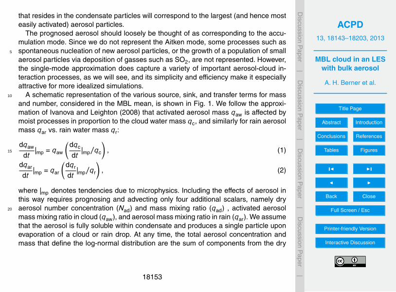
A schematic representation of the various source, sink, and transfer terms for mass10

and number, considered in the MBL mean, is shown in Fig. 1. We follow the approxi-mation of Ivanova and Leighton (2008) that activated aerosol mass qaw is affected bymoist processes in proportion to the cloud water mass qc, and similarly for rain aerosolmass qar vs. rain water mass qr:

dqaw

dt|mp = qaw

(dqc

dt|mp/qc

), (1)15

dqar

dt|mp = qar

(dqr

dt|mp/qr

), (2)

where |mp denotes tendencies due to microphysics. Including the effects of aerosol inthis way requires prognosing and advecting only four additional scalars, namely dryaerosol number concentration (Nad) and mass mixing ratio (qad) , activated aerosol20

mass mixing ratio in cloud (qaw), and aerosol mass mixing ratio in rain (qar). We assumethat the aerosol is fully soluble within condensate and produces a single particle uponevaporation of a cloud or rain drop. At any time, the total aerosol concentration andmass that define the log-normal distribution are the sum of components from the dry

18153





ACPD13, 18143–18203, 2013


A. H. Berner et al.

Title Page



Tables Figures

J I

J I

Back Close

Full Screen / Esc



Discussion

Paper

|D

iscussionP

aper|

Discussion

Paper

|D

iscussionP

aper|

(unactivated) aerosol, cloud droplets and rain drops:

Na = Nad +Nd +Nr, (3)

qa = qad +qaw +qar. (4)

Ivanova and Leighton included three modes in their scheme: unprocessed aerosol,5

cloud-processed aerosol, and a coarse mode resulting from evaporated precipitation.By simplifying their approach to a single accumulation mode, we keep the number ofauxiliary scalar fields to a minimum. We carry the aerosol mass mixing ratio in additionto number concentration for compatibility with the droplet activation parameterizationof Abdul-Razzak and Ghan (2000) used by the Morrison microphysics scheme (which10

requires these aerosol parameters), and compatibility with a newly developed scaveng-ing parameterization for interstitial aerosol. In the interstitial scheme, described furtherin the Appendix, scavenging tendencies for qad and Nad are computed using the cloudand raindrop size spectra from the Morrison scheme, together with approximate col-lection kernels for convective Brownian diffusion, thermophoresis, diffusiophoresis, tur-15

bulent coagulation, interception, and impaction. While interstitial scavenging has beenignored in several other studies, cloud droplets have a reasonably high collection effi-ciency for unactivated accumulation-mode aerosol (Zhang et al., 2004).

Surface fluxes are computed using a modified version of the wind-speed dependentsea salt parameterization of Clarke et al. (2006), where we have refit the size-resolved20

fluxes with a single, log-normal accumulation mode. As we are concerned mainly withparticles at sizes where they will be viable CCN, we choose to center the source dis-tribution about the geometric radius of 0.13 µm. To include the number and mass con-tributions from the smaller and most numerous portion of the coarse mode, as well asthe smallest end of the accumulation mode that may be active CCN at higher super-25

saturations, we choose a width parameter σg = 2. We then choose an aerosol numbersource that gives 50 % of the total integrated number flux in the distribution given byClarke et al. (2006); the remaining particles being assessed to be too small to act as

18154





ACPD13, 18143–18203, 2013


A. H. Berner et al.

Title Page



Tables Figures

J I

J I

Back Close

Full Screen / Esc



Discussion

Paper

|D

iscussionP

aper|

Discussion

Paper

|D

iscussionP

aper|

CCN.

dNad

dt|Srf = 1.706×102U10

3.41 m−2 s−1 (5)

dqad

dt|Srf = 2.734×10−19U10

3.41 kgm−2 s−1 (6)

The mass flux is only 0.5 % of that given by Clarke et al. (2006), for which the main5

mass flux is in large coarse-mode aerosols that again lie outside the range of sizesacross which our fit is optimized. Figure 2 plots the size-resolved mass and numberfluxes at a windspeed of 9 ms−1 for the Clarke et al. (2006) parameterization againstour unimodal approximation.

Aerosol in the free troposphere can be brought into the cloud layer through model-10

simulated entrainment. Observations suggest that over remote parts of the oceans, theFT generally has a substantial number concentration of aerosol particles that can actas CCN (e. g. Clarke, 1993; Clarke et al., 1996; Allen et al., 2011), but these particlesusually have diameters significantly smaller than 0.1 microns, and must grow via co-agulation and gas-phase condensation in the boundary layer before they activate into15

cloud droplets. Because we can not accurately represent this process, we short-circuitit by specifying a free-tropospheric aerosol number concentration comparable to mea-sured CCN concentrations, but by choosing these particles to already have a mean sizeof 0.1 micron and distribution width σg = 2, similar to what we assume for the surfaceaerosol source. Functionally, this is like assuming entrained aerosols instantaneously20

grow to this mean size by coagulation and gas-phase condensation when they enterthe boundary layer, a process which in reality may take hours to days (Clarke, 1993).This assumption also applies to the contribution of number from the surface source atsmaller sizes, which we consider as viable CCN when refitting the Clarke et al. (2006)parameterization to our single accumulation mode. Inclusion of nucleation from the gas25

phase and other chemistry is outside the scope of our idealized formulation.

18155





ACPD13, 18143–18203, 2013


A. H. Berner et al.

Title Page



Tables Figures

J I

J I

Back Close

Full Screen / Esc



Discussion

Paper

|D

iscussionP

aper|

Discussion

Paper

|D

iscussionP

aper|

The full system of equations governing the bulk aerosol moments in each grid cellare:

dNad

dt=

dNad

dt|Srf −

dNad

dt|Act −

dNad

dt|ScvCld −

dNad

dt|ScvRn +

dNd

dt|Evap +

dNr

dt|Evap

+dNad

dt|NMT (7)

dNd

dt=

dNad

dt|Act −

dNd

dt|Auto −

dNd

dt|Accr −

dNd

dt|Evap +

dNd

dt|NMT (8)5

dNr

dt=

dNd

dt|Auto −

dNr

dt|SlfC −

dNr

dt|Evap −

dNr

dt|Fallout +

dNr

dt|NMT (9)

dqad

dt=

dqad

dt|Srf −

dqad

dt|Act −

dqad

dt|ScvCld −

dqad

dt|ScvRn +

dqaw

dt|Evap +

dqar

dt|Evap

+dqad

dt|NMT (10)

dqaw

dt=

dqad

dt|Act +

dqad

dt|ScvCld −

dqaw

dt|Auto −

dqaw

dt|Accr −

dqaw

dt|Evap +

dqaw

dt|NMT (11)

dqar

dt=

dqaw

dt|Auto +

dqaw

dt|Accr +

dqad

dt|ScvRn −

dqar

dt|Evap −

dqar

dt|Fallout +

dqar

dt|NMT (12)10

Here subscript Srf denotes a surface flux, Act is CCN activation, ScvCld is interstitialscavenging by cloud droplets, ScvRn is interstitial scavenging by rain droplets, Evapis evaporation, Auto is autoconversion, Accr is accretion, SlfC is self-collection of rain,and NMT are non-microphysical terms (advection, large scale subsidence, and sub-15

grid turbulent mixing).The equations for Nd and Nr are identical to the standard implementations within

version 3 of the Morrison microphysics implemented in SAM v6.9, though the aerosolmass and number used within the Abdul-Razzak and Ghan activation parameterizationare now the local values of qa = qad +qaw and Nad +Nd, respectively. The equation for20

Nad also includes cloud and rain evaporation terms from the Morrison schemes, as well18156





ACPD13, 18143–18203, 2013


A. H. Berner et al.

Title Page



Tables Figures

J I

J I

Back Close

Full Screen / Esc



Discussion

Paper

|D

iscussionP

aper|

Discussion

Paper

|D

iscussionP

aper|

as contributions from the surface flux, interstitial scavenging, and advection/turbulence.The microphysical mass sources and sinks are derived from the corresponding Morri-son cloud and rain mass sources and sinks using the Ivanova–Leighton approximations(1) and (2). One modification was made to the Morrison scheme. The default schemeassumes no loss of cloud droplet number due to evaporation until all water is removed5

from a grid box (homogeneous mixing). This assumption has been replaced with theheterogeneous mixing assumption that cloud number is evaporated proportionately tocloud water mass, which theory and field measurements suggest may be more appro-priate for stratocumulus clouds (Baker et al., 1984; Burnet and Brenguier, 2007).

The discretized system preserves aerosol mass and number budgets within the do-10

main. The domain-integrated mass source and sink terms are due to surface flux ofqad, fallout of qar, and mean vertical advection. Aerosol number has a more complexbudget. One unforeseen complication was the limiter tendencies within the Morrisonmicrophysics code necessary to prevent unphysical rain and cloud droplet size dis-tributions. To conserve mass, the Morrison scheme adds or subtracts rain and cloud15

number to keep the droplet size distributions within observationally derived bounds.We maintain a closed aerosol budget under these conditions by shifting aerosol num-ber between Nr or Nd and Nad. A spurious source of total number (which we keep trackof) can still result from the rare case when the required droplet number source exceedsthe available dry aerosol number.20

2.2 Model domain, grid resolution, and boundary conditions

Most of the simulations were run in two dimensions, as the computational expense ofa 10–20 day run was unaffordable in 3-D with readily available resources. In Sect. 5.1,we compare two day periods from identically forced 2-D and 3-D cases, which showqualitatively similar behavior. Except where otherwise noted, 2-D runs use a 24 km25

wide periodic domain with 125 m horizontal resolution and 192 horizontal grid points,and a stretched vertical grid of 384 grid points, with spacing varying from 30 m at thesurface to 5 m in a layer from 200 m to 1500 m, then stretching to the domain top at

18157





ACPD13, 18143–18203, 2013


A. H. Berner et al.

Title Page



Tables Figures

J I

J I

Back Close

Full Screen / Esc



Discussion

Paper

|D

iscussionP

aper|

Discussion

Paper

|D

iscussionP

aper|

30 km (necessary for radiation). One domain-size sensitivity study uses a 96 km widedomain, and the POC runs discussed in Sect. 8 extend the 2-D grid to 192 km in width.The 3-D sensitivity study uses a 24km×24 km doubly-periodic domain. A dynamicaltime step of 0.5 s is used in all cases, adaptively shortened when necessary to avoidnumerical instability (an infrequent occurrence).5

3 Initialization and forcing

3.1 Temperature, moisture, and wind

The thermodynamic sounding and winds used in this study are loosely based on theVOCALS-RF06 derived profiles of Berner et al. (2011). Changes include a reductionof the inversion height to 1300 m from 1400 m and initial boundary layer qt reduced to10

7.0 gkg−1 from 7.5 gkg−1. This results in a thinner and less drizzly initial cloud layerthat does not deplete a large fraction of the initial aerosol during the spin-up of the sim-ulations. The wind is forced using a vertically uniform geostrophic pressure gradientand the initial sounding is tuned to minimize inertial oscillations. The free-troposphericmoisture and temperature are nudged to their initial profiles (or downward linear extrap-15

olations thereof, if the inversion shallows more than 150 m from its initial specification)on a one hour timescale in a layer beginning 150 m above the diagnosed inversionheight. The sounding and winds averaged over hour three of the control case are de-picted in Fig. 3.

3.2 Radiation20

Most simulations use diurnally averaged insolation and an insolation-weighted solarzenith angle appropriate for the latitude and time of year of the VOCALS-RF06 POCobservation. Section 6.2 presents a sensitivity study using a diurnal cycle of insolation.

18158





ACPD13, 18143–18203, 2013


A. H. Berner et al.

Title Page



Tables Figures

J I

J I

Back Close

Full Screen / Esc



Discussion

Paper

|D

iscussionP

aper|

Discussion

Paper

|D

iscussionP

aper|

3.3 Subsidence

Mean subsidence is assumed to increase linearly from the surface to a height of 3000 mand to be constant above that. Throughout this paper, the subsidence profile is in-dicated using its value at a height of 1500 m, which is between 4.75–6.5 mms−1 inthe simulations presented. These values are somewhat larger than our best guess of5

the actual mean subsidence at 1500 m during VOCALS-RF06 (2 mms−1; Wood et al.,2011b). This subsidence range was chosen because it exhibits an interesting rangeof cloud-aerosol-precipitation interaction and long-lived regimes under steady forcing.A simulation with the observed subsidence produces an initial evolution qualitativelysimilar to the first case discussed below, but with more rapid initial cloud deepening10

and onset of drizzle. In the VOCALS study region, there is a significant diurnal cycle ofsubsidence, but we have not included it here for simplicity, since in this paper our focusis on cloud-aerosol regimes which evolve mainly in response to the average forcingover longer periods of time.

3.4 Microphysics15

The aerosol number concentration in the FT is set to 100 mg−1, typical of FT CCNconcentrations over the remote ocean observed in VOCALS (Allen et al., 2011). A sen-sitivity test with no FT aerosol is discussed in Sect. 6.1. Within the MBL, cases withvertically-uniform initial aerosol concentrations ranging from 100 mg−1 to as low as10 mg−1 are considered, inspired by VOCALS-observed ranges within the MBL over20

the remote ocean (Allen et al., 2011).

4 Simulations and synopsis of results

Table 1 lists the simulations discussed in this paper and summarizes our naming con-vention. Slight random noise in the initial temperature field is used to initiate eddy mo-tions. Before discussing the results in detail, we provide a brief synopsis. In the base-25

18159





ACPD13, 18143–18203, 2013


A. H. Berner et al.

Title Page



Tables Figures

J I

J I

Back Close

Full Screen / Esc



Discussion

Paper

|D

iscussionP

aper|

Discussion

Paper

|D

iscussionP

aper|

line W5/NA100 run, the cloud layer deepens, thickens, and starts to drizzle, transitionsto open cellular convection via strong precipitation scavenging, and then collapses;this evolution is also found in a three-dimensional version of this run, as well as ina larger-domain 2-D simulation. If W is raised to 6.5 mms−1, the cloud layer deepeningis suppressed and a nearly nonprecipitating steady state stratocumulus layer develops.5

The early development of these runs is reminiscent of prior simulations of Mechemand Kogan (2003) and Wang et al. (2010). A similar bifurcation between cloud thick-ening and collapse vs. development of a steady state is seen when the diurnal cycleis included. For the W6.5 case, we also consider identically forced runs with differentinitial aerosol concentrations (NA50, NA30, NA10). The NA10 run evolves through an10

collapsing open-cell regime into a different thin-cloud equilibrium than the other runs.Finally, we consider “POC” simulations in a larger 2-D domain where the initial MBLaerosol includes a horizontal variation in initial MBL aerosol concentration. These runsproduce a low-aerosol open-cell state that develops from the initially lower Na region,but in the 100 : 50 run, the surrounding region remains a well-mixed, nearly nonprecip-15

itating stratocumulus topped boundary layer with higher aerosol concentrations; thisPOC-like combined state persists indefinitely given steady forcing.

The model behavior agrees qualitatively with observations in a number of importantrespects that increase our confidence in its applicability. In the VOCALS campaign,POCs were observed to form rapidly, almost always in the early morning hours when20

LWP reaches its maximum (Wood et al., 2011b, 2008). In the model, stable stratocumu-lus decks can persist with diurnally averaged LWPs up to around 100 gm−2, but largerLWPs result in precipitation sinks of aerosols that cannot be balanced by reasonablesource strengths. This agrees well with the LWP climatology of Wood and Hartmann(2006) for subtropical stratocumulus. The modeled transition from stratocumulus to25

open cells occurs via strong precipitation feedbacks, again in agreement with obser-vations (van Zanten and Stevens, 2005; Comstock et al., 2005; Wood et al., 2011b),and in an observationally reasonable period on the order of ten hours. The model alsoproduces a post-transition vertical structure for aerosol in good agreement with obser-

18160





ACPD13, 18143–18203, 2013


A. H. Berner et al.

Title Page



Tables Figures

J I

J I

Back Close

Full Screen / Esc



Discussion

Paper

|D

iscussionP

aper|

Discussion

Paper

|D

iscussionP

aper|

vations, with a surface layer Nad on the order of 20–30 mg−1 and a decoupled upperlayer with much lower values, including an “ultra-clean layer” as observed in VOCALSRF06 (Wood et al., 2011b).

5 Evolution through multiple cloud-aerosol regimes

We begin our analysis with run W5/NA100. Figure 4 depicts time-height plots of5

horizontally-averaged total (dry plus wet) aerosol number concentration and liquidwater content, as well as time series for important domain-averaged MBL meteoro-logical variables and for individual tendency terms from the MBL-averaged aerosolnumber budget. To compute the budget, terms are calculated between the surfaceand the time-varying horizontal-mean inversion height zi, determined as the height at10

which the domain mean relative humidity goes below 50 %. The entrainment source iswe(NaFT −NaMBL)/zi. Here we is the entrainment rate, diagnosed from the differencebetween the zi tendency and the mean vertical motion at the inversion height. Thisapproach is approximate, but the residual that it induces in the aerosol number budgetis only a few percent of the dominant terms. The scavenging of interstitial aerosol num-15

ber by rain is not shown on the aerosol number budget plot, because it never exceeds1 mg−1 day−1, which is much smaller than the terms shown.

The plots reveal three distinct regimes: an initial period with a well-mixedstratocumulus-topped boundary layer, a transitional period with decoupled verticalstructure, reduced cloud, and heavy precipitation, and a collapsed boundary layer state20

with continual weak precipitation and sharply reduced aerosol concentrations.Over the first two days, the inversion slowly deepens, the stratocumulus layer thick-

ens and its LWP increases. There is a 25 % decrease in Na despite relatively negligiblesurface precipitation. Figure 4d shows that over the first day, the dominant aerosol lossterm is interstitial scavenging by cloud, with smaller and roughly comparable losses25

from autoconversion and accretion, and a very small term due to aerosol number non-conservation from limiters within the microphysics scheme acting to keep the cloud size

18161





ACPD13, 18143–18203, 2013


A. H. Berner et al.

Title Page



Tables Figures

J I

J I

Back Close

Full Screen / Esc



Discussion

Paper

|D

iscussionP

aper|

Discussion

Paper

|D

iscussionP

aper|

distribution within defined bounds. These losses are balanced primarily by the surfacesource, with a slowly increasing contribution from entrainment. As noted by Mechemet al. (2006), the FT may act as a reservoir for MBL CCN when the MBL-averageCCN number concentration falls below that of the FT. During the second day, accretionlosses begin to rise more sharply, while interstitial scavenging by cloud diminishes. This5

occurs due to the improved collection efficiency for drizzle drops for constant qr anddiminishing Nr, while interstitial scavenging becomes less efficient as cloud dropletsgrow larger.

During day three, accretion losses grow to dominate the number budget, while Fig. 4cshows entrainment sharply declining as the domain-averaged surface precipitation10

rate climbs above 0.5 mmday−1. This is an example of what Feingold and Kreiden-weis (2002) called a “runaway precipitation process”. The decrease in entrainment isdue to a rapid decrease in turbulence near the top of the boundary layer, because ofdrizzle-induced stabilization of the boundary layer (Stevens et al., 1998) and reduceddestabilization by boundary-layer radiative cooling as cloud cover reduces. The result15

is a crash of MBL Na and a drastic reduction in LWP. Figure 4d shows the sink termsdiminish rapidly at the end of day three, primarily because the vast majority of aerosolhas been removed from the cloud layer.

The transition from well-mixed stratocumulus to showery, cumuliform dynamics isabrupt. Figure 5 shows x–z snapshots of ql and Na at three times spanning a six-20

teen hour period (day 2.625 to day 3.295). At the first time, cloud cover is essentially100 %, with ql maxima near 1 gkg−1 and a slight amount of cloud base drizzle underthe thickest clouds. Total aerosol concentration Na has only a slight vertical gradientand is about 40 mg−1 in the cloud layer. At the second time, eight hours later, the cloudis thinning and breaking towards the center of the domain, and in a smaller section25

of the domain there is surface precipitation beneath a strong drizzle cell with cloud-top ql in excess of 1.5 gkg−1. The decoupled structure of the boundary layer inhibitsaerosol transport from the surface layer into the remaining cloud. Hence, aerosol con-centration has become quite vertically stratified, with cloud layer values depleted near

18162





ACPD13, 18143–18203, 2013


A. H. Berner et al.

Title Page



Tables Figures

J I

J I

Back Close

Full Screen / Esc



Discussion

Paper

|D

iscussionP

aper|

Discussion

Paper

|D

iscussionP

aper|

or below 10 mg−1, except for higher values around the strong updraft of the drizzle cell.At the final time, cloud cover has fallen below 50 %; one weak drizzle cell remains, butthe cloud layer ql is nearly totally depleted. A narrow band of highly depleted aerosolconcentrations sits 100–300 m below the inversion, with concentrations falling below5 mg−1 (an “ultra-clean layer”), while the surface layer concentrations remain between5

20–30 mg−1. Referring back to Fig. 4d, the net MBL aerosol number sink rate duringthis 16 h period exceeds 60 mg−1 day−1, allowing for near complete aerosol depletionin less than 24 h.

The showery, cumuliform conditions following the sharp transition from stratocumu-lus persist for approximately two days. During this period, Fig. 4c shows that strong10

drizzle events occur periodically with spikes in surface precipitation up to 4 mmday−1,cloud cover oscillates around 60 % (much of which is optically thin), and domain-meanLWP oscillates between 20–40 gm−2. Entrainment is negligible, so the boundary layercontinually shallows and the cumulus cloud layer thins. During the sixth day, surfaceprecipitation becomes lighter and more continuous at around 1 mmday−1, while liquid15

water path falls to between 10–20 gm−2, as the cloud layer becomes too thin to supportepisodic cumulus showers. Figure 4a also suggests there is less vertical stratificationof the boundary layer aerosol. The boundary layer maintains this state while shallow-ing due to subsidence from a depth of 700 m down to 300 m. This slow boundary layercollapse is reminiscent of results from a one-dimensional turbulence closure modeling20

study of Ackerman et al. (1993).After six days of slow collapse, the MBL is sufficiently shallow and the inversion is

weak enough that thin cloud forms near the top of the boundary layer and reinvigo-rates entrainment. The sudden influx of entrained aerosol into the cloud decreasescloud droplet sizes, reducing precipitation efficiency and cloud processing sinks within25

the boundary layer. This results in a positive entrainment-cloud-aerosol feedback thatrapidly replenishes boundary layer aerosol, allowing the layer to sustain radiatively ac-tive cloud and begin deepening again via entrainment. While cloud type is initially thinSc, as the layer deepens the thin cloud is unable to develop sufficient turbulence to

18163





ACPD13, 18143–18203, 2013


A. H. Berner et al.

Title Page



Tables Figures

J I

J I

Back Close

Full Screen / Esc



Discussion

Paper

|D

iscussionP

aper|

Discussion

Paper

|D

iscussionP

aper|

mix the full layer depth, and a decoupled structure takes over with around day 10.5with lower cloud fraction, slightly reduced entrainment, and a larger vertical aerosolgradient.

The boundary layer continues to deepen and moisten over the next few days witha similar boundary layer structure. On day 15, entrainment begins to strengthen again5

due to larger LWP and radiatively driven turbulence; full cloud cover is achieved duringday 16. While Fig. 4 only extends 20 days, similar simulations we have run past 22 daysexhibit limit cycle behavior, collapsing again due to the runaway precipitation sink ofaerosol. In a sensitivity test using a 96 km wide domain (run W5/NA100/LD), mesoscalevariability allows a region of stratocumulus to form, begin replenishing MBL aerosol,10

and restart inversion deepening earlier in the collapse process, when the inversion isstill at a height of 700 m. This indicates the collapsed regime is fairly delicate in thismodel.

5.1 Comparison with 3-D results

To check the robustness of our 2-D results, we performed a two-day, 3-D simulation15

W5/NA100/3-D identical in forcing and initialization to the W5/NA100 case, except us-ing a domain of 24km×24km in horizontal extent. The evolution of this run comparedwith the 2-D control run is depicted in Fig. 6. A few differences are apparent. Entrain-ment in the 3-D simulation is less efficient than in the 2-D run; the boundary layer firstshallows during spin-up, then slowly deepens to a maximum of 1270 m after one day20

of evolution, while the 2-D run is nearly 50 m deeper at this point. This results in lessentrainment drying of the boundary layer, and a peak LWP of 175 gm−2 is reached inthe 3-D case as compared to a maximum of 155 gm−2 in the 2-D case. The transition toa collapsing state begins after only 24 h in the 3-D run, while taking 54 h to reach in the2-D case. This is due partly to the larger LWP accelerating precipitation losses, as well25

as the greater strength of cloud interstitial scavenging sink, which is nearly twice aslarge in the 3-D case. The combination of these effects leads to accelerated scaveng-

18164





ACPD13, 18143–18203, 2013


A. H. Berner et al.

Title Page



Tables Figures

J I

J I

Back Close

Full Screen / Esc



Discussion

Paper

|D

iscussionP

aper|

Discussion

Paper

|D

iscussionP

aper|

ing of aerosol within the boundary layer and faster onset of the runaway precipitationsink.

While the strengths of the aerosol number source and sink terms differ quantita-tively between the 2-D and 3-D configurations, their relative roles are similar. Interstitialscavenging is initially the largest sink of Na and the surface flux the largest source.5

As multiple processes act to reduce Na, the entrainment source strengthens, but isultimately unable to compete with the accretion losses as drizzle becomes significant.Cloud fraction decreases in both runs following the development of significant surfaceprecipitation and the rainout of ql, demonstrating qualitatively similar dynamics. As the3-D configuration is nearly 200 times as computationally expensive to run, we use the10

2-D framework for the remainder of our simulations to enable the long run times nec-essary to examine aerosol-cloud regimes and equilibrium states.

6 Stable equilibrium and sensitivity to forcing

In the W5/NA100 run, cloud breakup occurs when LWP increases enough to inducea runaway drizzle-aerosol loss feedback. This suggests that this transition might be15

suppressed if LWP remains sufficiently low. With this in mind, Case W6.5/NA100increases 1500 m subsidence to 6.5 mms−1, limiting LWP by inhibiting the bound-ary layer from deepening. This case, shown in Fig. 7, reaches a steady, well-mixed,stratocumulus-topped equilibrium state with an inversion height of 1100 m. LWP settlesto a mean of approximately 65 gm−2 after eight days, with oscillations of ±5 gm−2 about20

this value thereafter. The boundary layer Na settles around 88 mg−1, with 100 % cloudcover, less than 0.1 mmday−1 of cloud base drizzle and negligible precipitation reach-ing the surface. The steady state aerosol budget is dominated by an MBL-averagedsurface Na source of 20 day−1 and an interstitial scavenging Na sink of 12 day−1, withsmaller contributions from other processes.25

18165





ACPD13, 18143–18203, 2013


A. H. Berner et al.

Title Page



Tables Figures

J I

J I

Back Close

Full Screen / Esc



Discussion

Paper

|D

iscussionP

aper|

Discussion

Paper

|D

iscussionP

aper|

6.1 Sensitivity to FT aerosol

Case W6.5/NA100-0FT is identical to Case W6.5/NA100, except that the FT aerosolconcentration is set to zero. In this run, entrainment dilution is always a sink termfor MBL-mean Na. After a gradual depletion of aerosol, the run-away precipitation sinktransitions the system into a collapsed MBL. The simulation was run out to 20 days and5

remained in a collapsed state, with the inversion continually sinking slowly throughout(no plots shown).

6.2 Sensitivity to diurnal cycle of insolation

Case W5/NA100/DC (Fig. 8) is configured similarly to the control run W5/NA100,except with a diurnal cycle of insolation. Surprisingly, the inversion does not initially10

deepen as fast as in the control run, because the daily-mean entrainment rate is lower.This occurs because the cloud dissipates during the daytime, leading to a diurnally-averaged reduction in longwave cooling and turbulence compared to the control case.As a result, the cloud layer evolves towards a steady diurnal oscillation rather than thick-ening until it undergoes the runaway precipitation feedback. The cloud LWP exceeds15

200 gm−2 for a few hours at night, but this is not long enough for accretion losses tobuild up before the cloud thins during the daytime and aerosol regenerates. A curiousfeature of the case is a nearly 2 ms−1 oscillation in simulated surface wind speed, driv-ing a large simulated diurnal cycle in surface aerosol number flux(which is proportionalto the cube of the wind speed). This effect is attributed to reduced downward turbu-20

lent mixing of momentum to the surface layer during the daytime. Observational datashow a much weaker diurnal cycle in windspeed of a few tenths of a meter per second(Dai and Deser, 1999); we speculate that our 2-D approach is artificially amplifying thesimulated wind and surface aerosol flux oscillation, although we don’t think this hasa major impact on our results. The case was rerun with the 1500 m subsidence rate re-25

duced 5 % to 4.75 mms−1, and behavior similar to the control case reappears (Fig. 9).The rapid reduction in cloud LWP and cloud fraction occurs in the early morning when

18166





ACPD13, 18143–18203, 2013


A. H. Berner et al.

Title Page



Tables Figures

J I

J I

Back Close

Full Screen / Esc



Discussion

Paper

|D

iscussionP

aper|

Discussion

Paper

|D

iscussionP

aper|

precipitation is most active, as in the formation of observed POCs (Wood et al., 2008).The sensitivity of the long-term behavior to this slight change in an external parameteris an indicator of a positive-feedback system. The diurnal modulation of the terms inthe aerosol number budget does not seem to alter their relative importance in eachcloud regime compared to the control case.5

7 A reduced-order phase-plane description of the aerosol-cloud system

Schubert et al. (1979) discussed characteristic timescales on which a stratocumulus-capped mixed layer adjusts to a sudden change in boundary conditions and forcings.They pointed out that there is a quick (few hours) thermodynamic adjustment of theMBL, followed by a slower adjustment timescale (several days) for the MBL depth to ad-10

just into balance with the mean subsidence. Bretherton et al. (2010) elaborated theseideas using both mixed-layer modeling and LES of stratocumulus-capped boundarylayers with fixed cloud droplet concentrations. They showed that with fixed boundaryconditions, for any initial condition, the MBL evolution converged after thermodynamicadjustment onto a “slow manifold” along which the entire boundary-layer thermody-15

namic and cloud structure was slaved to a single slowly-evolving variable, the inversionheight (zi). With a cloud droplet concentration of 100 cm−3 they found there were twopossible slow manifolds, a “decoupled” manifold evolving toward a steady state withsmall cloud fraction and a shallow inversion, and a “well-mixed” manifold evolving to-ward an solid stratocumulus layer with a deep inversion. In both equilibria, precipita-20

tion was negligible. Simulations initialized with well-mixed boundary layers capped witha cloud layer that was optically thick but non-drizzling converged onto the well-mixedmanifold; simulations in which the initial cloud layer was either optically thin or so thickas to heavily drizzle converged onto the decoupled manifold.

In this section, we explore the use of similar concepts for our cloud-aerosol sys-25

tem. Given the MBL-average aerosol 〈Na〉, the clouds and turbulence will pattern theaerosol sources and sinks to set up the vertical structure of Na within the MBL within

18167





ACPD13, 18143–18203, 2013


A. H. Berner et al.

Title Page



Tables Figures

J I

J I

Back Close

Full Screen / Esc



Discussion

Paper

|D

iscussionP

aper|

Discussion

Paper

|D

iscussionP

aper|

its turbulent overturning time of a few minutes (for a coupled boundary layer) to a fewhours (for a decoupled boundary layer). Hence, the combination of 〈Na〉 and zi pro-vides a reduced-order two-dimensional phase-space to describe the “slow manifold”evolution of the cloud-aerosol system on timescales of a day or longer.

We start by viewing the control W5/NA100 case in this way. Figure 10 shows the5

position in 〈Na〉–zi phase space averaged over sequential 12 h periods, colored by theLWP during that period. The first 12 h adjustment period of the vertical structure of theboundary layer and the aerosol is shown in light grey, and the second in dark grey.The spacing between successive points indicates how fast a run is evolving. Differ-ent “regimes” through which the system evolves are labeled. Here, a cloud-aerosol10

regime is defined as a part of phase space with qualitatively similar cloud and aerosolcharacteristics, and hence different balances of terms in the aerosol budget. For in-stance, the open cell regime is characterized by low aerosol, low LWP, low entrainmentand efficient precipitation (accretion) removal of aerosol, while the thick cloud regimeis characterized by high aerosol, high LWP, little precipitation, high entrainment, and15

a balance between cloud scavenging and surface/entrainment aerosol sources. Theregimes grade into each other as 〈Na〉 and zi change; they need not have sharp bound-aries in phase space. The shading indicates two regions of phase-space in which theaerosol concentration evolves comparatively rapidly, either due to runaway precipitationfeedback, or due to rapid “runaway” entrainment of aerosol when the shallow boundary20

layer with open-cell convection redevelops thin inversion-base stratocumulus clouds.Overall, the phase space trajectory has converged onto a limit cycle in which it willindefinitely move between the thick-cloud, open-cell, and thin-cloud regimes.

It is even more interesting to examine the W6.5 case in this framework. The invertedtriangles in Fig. 11 show the W6.5/NA100 evolution in 〈Na〉–zi phase space. This run25

shows a slow decrease in zi, with an initial decrease of 〈Na〉, later changing to a slightincrease during the final approach to a “thick-cloud” steady state at zi = 1100 m and〈Na〉 = 88 mg−1.

18168





ACPD13, 18143–18203, 2013


A. H. Berner et al.

Title Page



Tables Figures

J I

J I

Back Close

Full Screen / Esc



Discussion

Paper

|D

iscussionP

aper|

Discussion

Paper

|D

iscussionP

aper|

We performed a sequence of runs identical to W6.5/NA100, but with the initial MBLaerosol concentration varied to 10, 30, and 50 mg−1; results are also plotted on Fig. 11.The simulations with initial Na values of 30 and 50 mg−1 (five and six pointed stars,respectively) evolve to the same thick-cloud equilibrium as the NA100 case. The initialzi drop is faster for lower 〈Na〉, because increased drizzle inhibits entrainment. After5

a few days, both simulations have settled to nearly their equilibrium zi but still slowlydrift toward higher 〈Na〉 as they approach the steady state.

The run with initial 〈Na〉 of 10 mg−1 (diamonds) immediately enters a runaway precip-itation feedback as it spins up, transitioning after the first 12 h to a low-LWP collapsingboundary layer. The “elbow” in the lower left corner of the phase space indicates a time10

at which the MBL eventually recovers a thin layer of stratocumulus and starts to rapidlyre-entrain aerosol, as in the W5/NA100 case. In contrast to that case, the stratocumu-lus layer never thickens enough to support vigorous turbulence, and the entrainmentis only able to slightly deepen the boundary layer, settling into a second stable “thin-cloud” equilibrium that is different than for the other initial conditions, with high 〈Na〉 and15

no drizzle.The labelled regimes occupy the same parts of phase space as for W5, because

the aerosol loss rate is not directly affected by the instantaneous mean subsidencerate. However, increased subsidence causes individual simulations to evolve throughphase space differently than for W5. On Fig. 11, we have sketched in some additional20

features whose exact structure we can only guess at. The grey and red dashed curvesindicates the upper and lower boundaries of attractor basin for the thick-cloud steadystate, i. e. all points in phase space from which the slowly-evolving system convergesto that steady state. Although the NA50 and NA30 runs appear to start outside thisattractor basin, note that it is only after the initial thermodynamic adjustment, which25

takes about a day, that the system behavior locks into this slowly-evolving phase-planedescription. By that time these runs are well within the notional boundary of the attractorbasin. The sketched arrow indicate the rough direction in which the system evolvesthrough different parts of phase space. Between the two steady states, the red dashed

18169





ACPD13, 18143–18203, 2013


A. H. Berner et al.

Title Page



Tables Figures

J I

J I

Back Close

Full Screen / Esc



Discussion

Paper

|D

iscussionP

aper|

Discussion

Paper

|D

iscussionP

aper|

curve separates trajectories for which the cloud thickens and the inversion deepenstoward the thick cloud equilibrium, and ones for which the cloud thins and the inversionshallows toward the thin cloud equilibrium. This is an example of sensitive dependenceof the long-term system evolution to its initial state. From the simulations we haveperformed, the open-cell regime is quite robust, so we anticipate that if 〈Na〉 is slightly5

larger than on this trajectory, it will adjust downward onto a similar trajectory as theNA10 simulation. For large zi > 1300 m, the W5/NA100 simulation suggest that LWP isvery large, increasing accretion loss of 〈Na〉. Thus we hypothesis that both the attractorboundary and the “runaway precipitation” area of very rapid aerosol depletion moverightward as zi increases. With an expanded set of runs that varies the initial zi in10

addition to 〈Na〉, the phase plane evolution could be filled out more confidently andprecisely.

The two equilibria of the W6.5 phase plane are strikingly similar to those found byBretherton et al. (2010). This suggests that there may be parts of phase space withtwo possible slow manifold behaviors, depending on the initial state of the system.15

However, unlike in Bretherton et al. (2010), initial states with very thick cloud will quicklyremove their aerosol through precipitation accretion, forcing them into a low-aerosolopen-cell state before returning back to the thin cloud equilibrium via runaway aerosolentrainment.

Unlike Baker and Charlson (1990), we do not find a high-aerosol and a low-aerosol20

steady state for W6.5. However, the open-cell regime is quite long-lived, and withoutfree-tropospheric aerosol, the runaway-entrainment transition to the thin cloud, high-aerosol equilibrium would not occur. Thus, our simulations are consistent in spirit withtheir hypothesis. In our work, however, interstitial aerosol removal is much more effi-cient, and entrainment dilution is active, regulating the high-aerosol state to number25

concentrations of around 100 mg−1, about ten times smaller than in their simple model.

18170





ACPD13, 18143–18203, 2013


A. H. Berner et al.

Title Page



Tables Figures

J I

J I

Back Close

Full Screen / Esc



Discussion

Paper

|D

iscussionP

aper|

Discussion

Paper

|D

iscussionP

aper|

8 POC simulations

So far, we have considered the evolution of an aerosol-cloud system in a small domainthrough multiple regimes over time, with the possibility of multiple steady states fora given forcing. We now examine the possibility of simultaneously supporting adjacentregions in different aerosol-cloud regimes in an idealized representation of a POC. We5

extend our domain to 192 km and specify an initial gradient in aerosol concentration,with a 42 km region initialized to Na

+, followed by a 12 km half-sine wave transition to84 km initialized at Na

−, then another half-sine wave transition back to 42 km initializedat Na

+. POC runs are initialized with identical thermodynamic profiles and forcings tothe W5/NA100 case. The idea is that the lower Na cloud within the center of the domain10

(the incipient POC) will start drizzling and transition via runaway precipitation feedbackto open cell structure. This will reduce entrainment in those regions. Because the in-version height in the open cell region must stay similar to that in the overcast region,reduced entrainment in part of the domain will slow or reverse inversion deepening overthe entire domain, as discussed in Berner et al. (2011). This can prevent the further15

growth of LWP and hence drizzle in the overcast region, and thereby suppress the tran-sition there, allowing a “coupled slow manifold” behavior hypothesized by Brethertonet al. (2010), in which the open-cell and overcast regions can stably coexist for longperiods.

Two pilot runs were tried using Na+ : Na

− of 30 : 25 and 60 : 40 mg−1, but as the20

simulated stratocumulus cloud layers deepened, the open-cell transition in the Na−

region was not complete before the Na+ regions also deepened sufficiently to transition.

However, in run W5/NA100:50-POC, initialized with Na+ : Na

− of 100 : 50 mg−1, theopen-cell transition in the domain center occurs sufficiently early to reduce the domain-mean zi and prevent the surrounding overcast region from transitioning. The remainder25

of this section documents this remarkable behavior.Figures 12 and 13 show x–z cross-sections of Na and ql at days 0.475 and 1.205.

In Fig. 12, the boundary layer is vertically well-mixed in Na and topped by an over-

18171





ACPD13, 18143–18203, 2013


A. H. Berner et al.

Title Page



Tables Figures

J I

J I

Back Close

Full Screen / Esc



Discussion

Paper

|D

iscussionP

aper|

Discussion

Paper

|D

iscussionP

aper|

cast stratocumulus layer. No significant drizzle is present, and no strong differencesother than the Na gradient are visible across the domain. Figure 13, 17.5 h later, showsa picture strongly reminiscent of observations from a POC, with several strong drizzlecells present in the central region and broken cloud. Na is highly depleted in places,falling below 15 mg−1 in the upper layer of the POC, and below 2 mg−1 in the bright ma-5

genta regions, nicely capturing the observed ultra-clean layer (Wood et al., 2011b). Thesurrounding overcast region maintains full cloud cover without substantial surface pre-cipitation, and Na remains above 75 mg−1 in the majority of the outer region. Anothermodel feature resembling observations of the VOCALS RF06 POC is the location of thehorizontal Na gradient, with the bulk of the aerosol decrease located within the overcast10

region (Wood et al., 2011b). The qualitative similarity to key features in the observa-tions suggests the simple model captures at least some of the important mechanismsin the real system.

After transition, the POC and overcast regions evolve jointly over the next severaldays, linked together by circulations acting to maintain an essentially level domain-15

wide inversion against large differences in entrainment and thermodynamic profilesbetween the overcast and POC regions. Figure 14 depicts Hovmöller plots of 〈Na〉 andLWP. The spatial evolution of the aerosol and LWP fields in Fig. 14a and b shows howthe POC initially widens rapidly following transition. The different character of the re-gions is apparent in Fig. 14b, in that the domain maximum and minimum LWP values20

are contained within the POC, while the overcast region is much more homogeneous.Figure 14a shows the degree to which the aerosol gradient is sharpened and main-tained by cloud processing. Interestingly, after its initial expansion, the POC reachesa maximum of 70 % of the domain on day 2.4, then shrinks back into a quasi-steadyequilibrium with the overcast by the time the run ends on day 9, occupying 25–30 % of25

the total area.In order to understand the apparent equilibration, we plot time series of several vari-

ables from averages over 24 km wide stripes at the center of each region in Fig. 15.In Fig. 15a, the transition to open cellular convection within the POC at the end of

18172





ACPD13, 18143–18203, 2013


A. H. Berner et al.

Title Page



Tables Figures

J I

J I

Back Close

Full Screen / Esc



Discussion

Paper

|D

iscussionP

aper|

Discussion

Paper

|D

iscussionP

aper|

the first day is evident, with a sharp decrease of 〈Na〉 there and corresponding lossof cloud fraction (Fig. 15f); within the overcast region, 〈Na〉 diminishes less rapidly. In-version heights fall in both regions after the transition, as depicted in Fig. 15b. This isa response to the reduced domain-mean entrainment resulting from the growth of thePOC, shown in Fig. 15c. The falling inversion thins the stratocumulus clouds, reducing5

LWP (Fig. 15d) and cloud processing of aerosol in the overcast region, in turn allowing〈Na〉 to increase. This further limits precipitation sinks of both aerosol and cloud wa-ter, and overcast LWP begins to recover soon after surface precipitation ceases on daythree. The inversion height and LWP then increase in unison, and as the cloud thickens,stronger cloud processing and buffering by entrainment dilution (Mechem et al., 2006)10

arrests the growth of overcast 〈Na〉. This suggests a negative feedback loop, where thecoupling between POC area, domain mean entrainment, and LWP as moderated by zistabilizes the system.

Figure 16 shows the nearly equilibrated behavior on day 9.58. Strong latent heatingin the upper region of the POC contrasts with continuous radiative cooling of the well15

mixed overcast. We hypothesize the 50 m difference in inversion height between thePOC and surrounding overcast represents a balanced response to this gradient in ver-tically integrated buoyancy. While the POC has diminished in area, drizzle processesare still very active. The cloudbase smoothly drops from the edges of the overcast, re-flecting the cooler, decoupled POC surface layer, and only the most active drizzle cells20

have cloud top heights near the inversion. Without the surrounding overcast region, theinversion in the POC region would have collapsed several hundred meters due to thelack of entrainment, while that in the overcast region would have deepened due to thelarge entrainment there and undergone runaway precipitation feedback, as in Fig. 4.That is, each region holds the other in balance.25

Interpreting this system in a reduced-complexity slow-manifold framework, the quasi-equilibrium evolution of each region is controlled its mean 〈Na〉 and by the coupledevolution of inversion height, i. e. domain-mean entrainment, which is in turn set, tofirst order, by the areal fraction of the domain occupied by the overcast region vs.

18173





ACPD13, 18143–18203, 2013


A. H. Berner et al.

Title Page



Tables Figures

J I

J I

Back Close

Full Screen / Esc



Discussion

Paper

|D

iscussionP

aper|

Discussion

Paper

|D

iscussionP

aper|

the POC. It is unclear exactly what controls the areal fraction of POC to overcast, butreduced POC entrainment couples to domain-wide boundary layer depth, LWP, andaerosol tendencies in a manner that creates a negative feedback on the horizontalexpansion of the POC.

9 Conclusions5

We have implemented a new single log-normal mode, double-moment bulk aerosolscheme coupled to the Morrison microphysics parameterization for the SAM LES.The scheme follows the general approach of Ivanova and Leighton (2008), though wehave used only a single dry mode for simplicity and computational efficiency. We usethis framework to examine the evolution of the cloud-aerosol system through different10

regimes, sensitivity to forcing and initial conditions, and the formation and equilibriumof POCs.

As in some past studies, transition from closed-cell stratocumulus to more cumuli-form, open-cellular convection occurs via the sharp enhancement of the accretion sinkas LWP increases and Nd decreases. If LWP does not get sufficiently high, this tran-15

sition never takes place. With diurnally-varying insolation, the transition occurs in theearly-morning hours, as with observed POC formation.

A series of identically forced runs varying the initial boundary layer aerosol con-centration demonstrated multiple equilibria, with higher Na runs settling into a deeper,well-mixed state and a run initialized with Na of 10 mg−1 transitioning to a collapsed20

boundary layer before recovering to a shallower layer with very thin cloud and little liq-uid water content and high Nd. A 2-D phase plane representation of the evolution ofthe cloud-aerosol system in terms of boundary-layer mean aerosol concentration andinversion height provides a convenient way to identify cloud-aerosol regimes and tran-sitions between them, and basins of attraction to the respective equilibria. In spirit, our25

results support the bistability hypothesis of Baker and Charlson (1990), though modi-

18174





ACPD13, 18143–18203, 2013


A. H. Berner et al.

Title Page



Tables Figures

J I

J I

Back Close

Full Screen / Esc



Discussion

Paper

|D

iscussionP

aper|

Discussion

Paper

|D

iscussionP

aper|

fied in important ways by entrainment feedback and interstitial aerosol scavenging bycloud droplets.

Another series of runs used a larger domain with a horizontal aerosol gradient toexplore the formation of POCs. When initialized with an outer domain Na of 100 mg−1

and an inner Na of 50 mg−1, the inner region transitioned to open-cellular cumuliform5

convection while the outer region remained well-mixed, closed-cell stratocumulus. Thetransition of the inner region reduced domain averaged entrainment, reducing the over-all inversion height and reducing cloud thickness and LWP in the outer region, resultingin increased Na there and providing a negative feedback on growth of the open-cellularregion. The resulting POC-overcast system appears to be a stable steady state under10

constant forcing. This is consistent with the observed robustness of POCs, which arerarely observed to close up once formed (Wood et al., 2008).

Future work will involve continued exploration of the phase space in an effort tomore fully map the behavior of the system, including longer three dimensional runs.Three-dimensional POC simulations will allow for the development of more complete15

regional aerosol budgets, particularly characterizing the role of horizontal transport ofaerosol from the overcast into the POC. Another area of potential research involvesthe sensitivity of nascent and fully developed POCs to FT aerosol perturbations, as thequestion of whether it is possible to close a POC remains open.

18175





ACPD13, 18143–18203, 2013


A. H. Berner et al.

Title Page



Tables Figures

J I

J I

Back Close

Full Screen / Esc



Discussion

Paper

|D

iscussionP

aper|

Discussion

Paper

|D

iscussionP

aper|

Appendix A

Interstitial Scavenging

A log-normal form f (A) is assumed for the aerosol size spectrum. The number andmass scavenging tendencies are:

∂n∂t

=∂∂t

∞∫0

f (A)dA = −∞∫0

γ(A)f (A)dA (A1)5

∂q∂t

=πρa

6∂∂t

∞∫0

A3f (A)dA = −πρa

6

∞∫0

γ(A)A3f (A)dA (A2)

where A is the aerosol diameter, ρa is aerosol density, and γ(A) is the scavengingcoefficient (e.g. Seinfeld and Pandis, 1998)

γ(d ) =π4

∞∫0

(D+A)2(U(D)−u(A))E (D,A)F (D)dD10

where D is the collecting drop diameter, U(D) and u(A) are the respective terminalfall speeds for the collecting drop and aerosol, F (D) is the size distribution of collectordrops, and E (D,A) is the collection efficiency. We approximate γ(A) by assuming theaerosol diameter and terminal velocity are much smaller than the collector drop diam-

eter and terminal velocity u(A). The collector fall speed has the form U = aDb(ρ0/ρ)1/215

(Khvorostyanov and Curry, 2002). The collector drop size distribution is assumed to fol-low a generalized gamma distribution F (D) = N0D

νexp(−λD), where N0 is the interceptparameter, ν the shape parameter, and λ is the slope parameter (e.g. Ulbrich, 1983).

18176





ACPD13, 18143–18203, 2013


A. H. Berner et al.

Title Page



Tables Figures

J I

J I

Back Close

Full Screen / Esc



Discussion

Paper

|D

iscussionP

aper|

Discussion

Paper

|D

iscussionP

aper|

With the above simplifications, the scavenging coefficient becomes:

γ(d ) =πa N0

4

∞∫0

D2+b+νE (D,A)exp(−λD)dD (A3)

In Morrison et al. (2005) and other double moment schemes, N0 and λ may be calcu-lated from the total number (Nd for cloud, Nr for rain) and water mass (qc for cloud, qrfor rain)5

N0 =Nλν+1

Γ(ν+1)

λ =[πρwN

6q(ν+3)(ν+2)(ν+1)

]1/3

where ρw is the density of water.Collision efficiency is given as the effective collision kernel over the geometric colli-10

sion kernel, approximated as

E (D,A) ≈K (D,A)π4D

2U(D),

where K (D,A) is the sum of the individual process kernels. For cloud droplets, theincluded processes are Brownian diffusion, thermophoresis, diffusiophoresis, and tur-bulent coagulation (using Pruppacher and Klett, 1997, Eqs. (11-59), (17-25), (17-33),15

and (11-77), respectively). The turbulent kernel currently assumes a fixed value for dis-sipation in convective clouds of ε = 4.22×10−5 m2 s−3; this will be updated to use thelocal model values of epsilon in future versions. For rain, K (D,A) is the semi-empiricalformulation of Slinn (1983). Appropriate values of sulfate aerosol thermal conductivityfor these kernels may be found in Seinfeld and Pandis (1998, p. 481). Figure 17 plots20

18177





ACPD13, 18143–18203, 2013


A. H. Berner et al.

Title Page



Tables Figures

J I

J I

Back Close

Full Screen / Esc



Discussion

Paper

|D

iscussionP

aper|

Discussion

Paper

|D

iscussionP

aper|

logE (D,A) for aerosol diameter vs. hydrometeor diameter at a pressure of 900 mb,temperature of 282 K, and relative humidity (RH) of 100.5 %. There is some sensitivityto logE (D,A) around RH values near 100 % for aerosol larger than 0.1 µm and clouddroplets between 5–20 µm; as the version of SAM used here does not include prog-nostic supser-saturation, we choose an in-cloud value of 100.5 %. The discontinuity at5

D = 80 µm shows the transition between cloud and rain kernels. Since collision efficien-cies for larger hydrometeors and accumulation mode (sub-micron diameter) aerosolare small (mostly below 1 %), this discontinuity is of little concern. The number andmass scavenging rates (A1) and (A2) are integrated numerically in a method general-izing the approach of Berthet et al. (2010).10

Look-up tables of γ(A) for cloud and rain as a function of temperature, pressure, RH,and cloud/rain precipitation fluxes are generated on initialization of the scheme. This isdone by integrating A3 across a default gamma distribution for cloud and the Marshall–Palmer distribution for rain using Gauss–Laguerre quadrature. Gauss–Hermite quadra-ture is then used to integrate over the aerosol size distribution using the current values15

of Na, qa, and look-up values of γ(A) to calculate the scavenging tendencies of Na andqa. For efficiency, the tendencies are updated once every three timesteps and are setto zero after all liquid or aerosol has been removed from a gridbox between updates.Future versions of the code will use the prognostic Morrison cloud and rain distributionswhen numerically integrating (A3) and include an option to calculate tendencies using20

an approximate analytical approach.

Acknowledgements. Thanks to Peter Blossey at UW for help with the implementation and de-bugging of the aerosol scheme. We are also grateful to Marat Khairoutdinov of Stony BrookUniversity for maintaining and providing SAM for use in this study. The authors gratefully ac-knowledge support from NSF grants ATM-0745702 and AGS-1242639 and the University of25

Washington College of the Environment Geoengineering Initiative.

18178





ACPD13, 18143–18203, 2013


A. H. Berner et al.

Title Page



Tables Figures

J I

J I

Back Close

Full Screen / Esc



Discussion

Paper

|D

iscussionP

aper|

Discussion

Paper

|D

iscussionP

aper|

References

Abdul-Razzak, H. and Ghan, S. J.: A parameterization of aerosol activation: 2. Multiple aerosoltypes, J. Geophys. Res., 105, 6837–6844, 2000. 18154

Ackerman, A. S., Toon, O. B., and Hobbs, P. V.: Dissipation of marine stratiform clouds andcollapse of the marine boundary layer due to the depletion of cloud condensation nuclei by5

clouds, Science, 262, 226–229, doi:10.1126/science.262.5131.226, 1993. 18163Ackerman, A. S., Toon, O. B., and Hobbs, P. V.: Reassessing the dependence of

cloud condensation nucleus concentration on formation rate, Nature, 367, 445–447,doi:10.1038/367445a0, 1994. 18146

Ackerman, A., Toon, O. B., Stevens, D. E., and Coakley Jr., J. A.: Enhancement of cloud cover10

and suppression of nocturnal drizzle in stratocumulus polluted by haze, Geophys. Res. Lett.,30, 1381, doi:10.1029/2002GL016634, 2003. 18147

Ackerman, A., Kirkpatrick, M. P., Stevens, D. E., and Toon, O. B.: The impact of humidity abovestratiform clouds on indirect aerosol climate forcing, Nature, 432, 1014–1017, 2004. 18148

Albrecht, B. A.: Aerosols, cloud microphysics, and fractional cloudiness, Science, 245, 1227–15

1230, 1989. 18146Allen, G., Coe, H., Clarke, A., Bretherton, C., Wood, R., Abel, S. J., Barrett, P.,

Brown, P., George, R., Freitag, S., McNaughton, C., Howell, S., Shank, L., Kapustin, V.,Brekhovskikh, V., Kleinman, L., Lee, Y.-N., Springston, S., Toniazzo, T., Krejci, R.,Fochesatto, J., Shaw, G., Krecl, P., Brooks, B., McMeeking, G., Bower, K. N., Williams, P. I.,20

Crosier, J., Crawford, I., Connolly, P., Allan, J. D., Covert, D., Bandy, A. R., Russell, L. M.,Trembath, J., Bart, M., McQuaid, J. B., Wang, J., and Chand, D.: South East Pacific atmo-spheric composition and variability sampled along 20◦ S during VOCALS-REx, Atmos. Chem.Phys., 11, 5237–5262, doi:10.5194/acp-11-5237-2011, 2011. 18155, 18159

Baker, M. B. and Charlson, R. J.: Bistability of CCN concentrations and thermodynamics in the25

cloud-topped boundary layer, Nature, 345, 142–145, 1990. 18146, 18170, 18174Baker, M. B., Breidenthal, R. E., Choularton, T. W., and Latham, J.: The ef-

fects of turbulent mixing in clouds, J. Atmos. Sci., 41, 299–304, doi:10.1175/1520-0469(1984)041<0299:TEOTMI>2.0.CO;2, 1984. 18157

Berner, A. H., Bretherton, C. S., and Wood, R.: Large-eddy simulation of mesoscale dynamics30

and entrainment around a pocket of open cells observed in VOCALS-REx RF06, Atmos.

18179





http://dx.doi.org/10.1126/science.262.5131.226

http://dx.doi.org/10.1038/367445a0

http://dx.doi.org/10.1029/2002GL016634

http://dx.doi.org/10.5194/acp-11-5237-2011

http://dx.doi.org/10.1175/1520-0469(1984)041<0299:TEOTMI>2.0.CO;2



ACPD13, 18143–18203, 2013


A. H. Berner et al.

Title Page



Tables Figures

J I

J I

Back Close

Full Screen / Esc



Discussion

Paper

|D

iscussionP

aper|

Discussion

Paper

|D

iscussionP

aper|

Chem. Phys., 11, 10525–10540, doi:10.5194/acp-11-10525-2011, 2011. 18148, 18158,18171

Berthet, S., Leriche, M., Pinty, J.-P., Cuesta, J., and Pigeon, G.: Scavenging ofaerosol particles by rain in a cloud resolving model, Atmos. Res., 96, 325–336,doi:10.1016/j.atmosres.2009.09.015, 2010. 181785

Blossey, P. N. and Durran, D. R.: Selective monotonicity preservation in scalar advection, J.Comp. Physiol., 227, 5160–5183, doi:10.1016/j.jcp.2008.01.043, 2008. 18152

Bony, S. and DuFresne, J.-L.: Marine boundary layer clouds at the heart of tropi-cal cloud feedback uncertainties in climate models, Geophys. Res. Lett., 32, 2–5,doi:10.1029/2005GL023851, 2005. 1814510

Burnet, F. and Brenguier, J.-L.: Observational study of the entrainment-mixing process in warmconvective clouds, J. Atmos. Sci., 64, 1995–2011, doi:10.1175/JAS3928.1, 2007. 18157

Bretherton, C. S., Uttal, T., Fairall, C. W. , Yuter, S., Weller, R., Baumgardner, D., Comstock, K.,and Wood, R.: The EPIC 2001 stratocumulus study, B. Am. Meteorol. Soc., 85, 967–977,2004. 1814715

Bretherton, C. S., Blossey, P. N., and Uchida, J.: Slow manifolds and multiple equi-libria in stratocumulus-capped boundary layers, J. Adv. Model. Earth Syst., 2, 14,doi:10.3894/JAMES.2010.2.14, 2010. 18151, 18167, 18170, 18171

Clarke, A. D.: Atmospheric nuclei in the Pacific midtroposphere: their nature, concentration, andevolution, J. Geophys. Res., 98, 20633, doi:10.1029/93JD00797, 1993. 1815520

Clarke, A. D., Li, Z., and Litchy, M.: Aerosol dynamics in the equatorial Pacific marine boundarylayer: Microphysics, diurnal cycles and entrainment, Geophys. Res. Lett., 23, 733–736, 1996.18155

Clarke, A. D., Owens, S. R., and Zhou, J.: An ultrafine sea-salt flux from breaking waves: impli-cations for cloud condensation nuclei in the remote marine atmosphere, J. Geophys. Res.,25

111, 1–14, doi:10.1029/2005JD006565, 2006. 18154, 18155, 18188Comstock, K., Bretherton, C. S., and Yuter, S.: Mesoscale variability and drizzle in Southeast

Pacific stratocumulus, J. Atmos. Sci., 62, 3792–3807, 2005. 18147, 18160Comstock, K. K., Yuter, S. E., Wood, R., and Bretherton, C. S.: The three-dimensional

structure and kinematics of drizzling stratocumulus, Mon. Weather Rev., 135, 3767–3784,30

doi:10.1175/2007MWR1944.1, 2007. 18147Dai, A. and Deser, C.: Diurnal and semidiurnal variations in global surface wind and divergence

fields, J. Geophy. Res., 104, 31109, doi:10.1029/1999JD900927, 1999. 18166

18180






http://dx.doi.org/10.1016/j.atmosres.2009.09.015

http://dx.doi.org/10.1016/j.jcp.2008.01.043

http://dx.doi.org/10.1029/2005GL023851

http://dx.doi.org/10.1175/JAS3928.1

http://dx.doi.org/10.1029/93JD00797

http://dx.doi.org/10.1029/2005JD006565

http://dx.doi.org/10.1175/2007MWR1944.1

http://dx.doi.org/10.1029/1999JD900927

ACPD13, 18143–18203, 2013


A. H. Berner et al.

Title Page



Tables Figures

J I

J I

Back Close

Full Screen / Esc



Discussion

Paper

|D

iscussionP

aper|

Discussion

Paper

|D

iscussionP

aper|

Deardorff, J.: Stratocumulus-capped mixed layers derived from a three-dimensional model,Bound.-Lay. Meteorol., 18, 495–527, 1980. 18152

Feingold, G.: Modeling of the first indirect effect: Analysis of measurement requirements, Geo-phys. Res. Lett., 30, 1–4, doi:10.1029/2003GL017967, 2003. 18150

Feingold, G. and Kreidenweis, S. M.: Cloud processing of aerosol as modeled by a large eddy5

simulation with coupled microphysics and aqueous chemistry, J. Geophys. Res., 107, 4687,doi:10.1029/2002JD002054, 2002. 18149, 18162

Feingold, G., Kreidenweis, S. M., Stevens, B., and Cotton, W. R.: Numerical simulations of stra-tocumulus processing of cloud condensation nuclei through collision-coalescence, J. Geo-phys. Res., 101, 21391, doi:10.1029/96JD01552, 1996. 1814910

Feingold, G., Koren, I., Wang, H., Xue, H., and Brewer, W. A.: Precipitation-generated oscilla-tions in open cellular cloud fields, Nature, 466, 849–852, doi:10.1038/nature09314, 2010.

Flossmann, A. I., Hall, W. D., and Pruppacher, H. R.: A theoretical study of the wet removalof atmospheric pollutants. Part I: The redistribution of aerosol particles captured throughnucleation and impaction scavenging by growing cloud drops, J. Atmos. Sci., 42, 583–606,15

doi:10.1175/1520-0469(1985)042<0583:ATSOTW>2.0.CO;2, 1985. 18149Hartmann, D. L., Ockert-Bell, M. E. and Michelsen, M. L.: The effect of cloud type on Earth’s

energy balance: Global analysis, J. Climate, 5, 1281–1304, 1992. 18145Ivanova, I. T. and Leighton, H. G.: Aerosol–cloud interactions in a mesoscale model.

Part I: Sensitivity to activation and collision–coalescence, J. Atmos. Sci., 65, 289–308,20

doi:10.1175/2007JAS2207.1, 2008. 18149, 18150, 18153, 18174Kazil, J., Wang, H., Feingold, G., Clarke, A. D., Snider, J. R., and Bandy, A. R.: Modeling

chemical and aerosol processes in the transition from closed to open cells during VOCALS-REx, Atmos. Chem. Phys., 11, 7491–7514, doi:10.5194/acp-11-7491-2011, 2011. 18149,1815025

Khairoutdinov, M. F. and Kogan, Y. L.: A new cloud physics parameterization in a large-eddy simulation model of marine stratocumulus, Mon. Weather Rev., 128, 229–243,doi:10.1175/1520-0493(2000)128<0229:ANCPPI>2.0.CO;2, 2000.

Khairoutdinov, M. F. and Randall, D. A.: Cloud resolving modeling of the ARM summer 1997IOP: model formulation, results, uncertainties, and sensitivities, J. Atmos. Sci., 60, 607–625,30

2003. 18151

18181





http://dx.doi.org/10.1029/2003GL017967

http://dx.doi.org/10.1029/2002JD002054


http://dx.doi.org/10.1175/1520-0469(1985)042<0583:ATSOTW>2.0.CO;2

http://dx.doi.org/10.1175/2007JAS2207.1


http://dx.doi.org/10.1175/1520-0493(2000)128<0229:ANCPPI>2.0.CO;2

ACPD13, 18143–18203, 2013


A. H. Berner et al.

Title Page



Tables Figures

J I

J I

Back Close

Full Screen / Esc



Discussion

Paper

|D

iscussionP

aper|

Discussion

Paper

|D

iscussionP

aper|

Khvorostyanov, V. I. and Curry, J. A.: Terminal velocities of droplets and crystals: powerlaws with continuous parameters over the size spectrum, J. Atmos. Sci., 59, 1872–1884,doi:10.1175/1520-0469(2002)059<1872:TVODAC>2.0.CO;2, 2002. 18176

Kollias, P. , Fairall, C. W., Zuidema, P., Tomlinson, J., and Wick, G. A.: Observations of marinestratocumulus in SE Pacific during the PACS 2003 cruise, Geophys. Res. Lett., 31, L22110,5

doi:10.1029/2004GL020751, 2004.MacCready, P. B.: The inertial subrange of atmospheric turbulence, J. Geophys. Res., 67, 1051,

doi:10.1029/JZ067i003p01051, 1962.Mechem, D. B. and Kogan, Y. L.: Simulating the transition from drizzling marine stratocumulus

to boundary layer cumulus with a mesoscale model, Mon. Weather Rev., 131, 2342–2360,10

doi:10.1175/1520-0493(2003)131<2342:STTFDM>2.0.CO;2, 2003. 18148, 18149, 18151,18160

Mechem, D. B., Robinson, P. C., and Kogan, Y. L.: Processing of cloud condensation nu-clei by collision-coalescence in a mesoscale model, J. Geophys. Res., 111, D18204,doi:10.1029/2006JD007183, 2006. 18148, 18162, 1817315

Mlawer, E. J., Taubman, S. J., Brown, P. D., Iacono, M. J., and Clough, S. A.: Radiative transferfor inhomogeneous atmospheres: RRTM, a validated correlated-k model for the longwave, J.Geophys. Res., 102, 16663, doi:10.1029/97JD00237, 1997. 18152

Morrison, H. and Grabowski, W. W.: Modeling supersaturation and subgrid-scalemixing with two-moment bulk warm microphysics, J. Atmos. Sci., 65, 792–812,20

doi:10.1175/2007JAS2374.1, 2008. 18152Morrison, H., Curry, J. A., and Khvorostyanov, V. I.: A new double-moment microphysics pa-

rameterization for application in cloud and climate models. Part I: Description, J. Atmos. Sci.,62, 1665–1677, doi:10.1175/JAS3446.1, 2005. 18150, 18152, 18177

Petters, M. D., Snider, J. R., Stevens, B., Vali, G., Faloona, I., and Russell, L. M.: Accumulation25

mode aerosol, pockets of open cells, and particle nucleation in the remote subtropical Pacificmarine boundary layer, J. Geophys. Res., 111, D02206, doi:10.1029/2004JD005694, 2006.18147

Pruppacher, H. R. and Klett, J. D.: Microphysics of Clouds and Precipitation, Kluwer AcademicPublishers, Dordrecht, Boston, London, 954 pp., 1997. 1817730

Quaas, J., Ming, Y., Menon, S., Takemura, T., Wang, M., Penner, J. E., Gettelman, A.,Lohmann, U., Bellouin, N., Boucher, O., Sayer, A. M., Thomas, G. E., McComiskey, A., Fein-gold, G., Hoose, C., Kristjánsson, J. E., Liu, X., Balkanski, Y., Donner, L. J., Ginoux, P. A.,

18182





http://dx.doi.org/10.1175/1520-0469(2002)059<1872:TVODAC>2.0.CO;2

http://dx.doi.org/10.1029/2004GL020751

http://dx.doi.org/10.1029/JZ067i003p01051

http://dx.doi.org/10.1175/1520-0493(2003)131<2342:STTFDM>2.0.CO;2

http://dx.doi.org/10.1029/2006JD007183



http://dx.doi.org/10.1175/JAS3446.1

http://dx.doi.org/10.1029/2004JD005694

ACPD13, 18143–18203, 2013


A. H. Berner et al.

Title Page



Tables Figures

J I

J I

Back Close

Full Screen / Esc



Discussion

Paper

|D

iscussionP

aper|

Discussion

Paper

|D

iscussionP

aper|

Stier, P., Grandey, B., Feichter, J., Sednev, I., Bauer, S. E., Koch, D., Grainger, R. G.,Kirkevåg, A., Iversen, T., Seland, Ø., Easter, R., Ghan, S. J., Rasch, P. J., Morrison, H.,Lamarque, J.-F., Iacono, M. J., Kinne, S., and Schulz, M.: Aerosol indirect effects – generalcirculation model intercomparison and evaluation with satellite data, Atmos. Chem. Phys., 9,8697–8717, doi:10.5194/acp-9-8697-2009, 2009. 181455

Savic-Jovcic, V. and Stevens, B.: The structure and mesoscale organization of precipitatingstratocumulus, J. Atmos. Sci., 65, 1587–1605, 2008. 18148

Seifert, A. and Beheng, K. D.: A double-moment parameterization for simulating autocon-version, accretion and selfcollection, Atmos. Res., 59–60, 265–281, doi:10.1016/S0169-8095(01)00126-0, 2001.10

Seinfeld, J. H. and Pandis, S. N.: Atmospheric Chemistry and Physics, John Wiley and Sons,605 Third Avenue, New York, NY, 1998. 18176, 18177

Schubert, W. H., Wakefield, J. S., Steiner, E. J. and Cox, S. K.: Marine stratocumulus convec-tion. Part I: Governing equations and horizontally homogeneous solutions, J. Atmos. Sci.,36, 1286–1307, 1979. 1816715

Slinn, W. G. N.: Precipitation scavenging, in: Atmospheric Sciences and Power Production –1979, chap. 11, Division of Biomedical Environmental Research, US Department of Energy,Washington, DC, 1983. 18177

Stevens, B., Cotton, W. R., Feingold, G., and Moeng, C.-H.: Large-eddy simulations of stronglyprecipitating, shallow, stratocumulus-topped boundary layers, J. Atmos. Sci., 55, 3616–3638,20

doi:10.1175/1520-0469(1998)055<3616:LESOSP>2.0.CO;2, 1998. 18162Stevens, B., Lenschow, D. H., Vali, G., Gerber, H., Bandy, A., Blomquist, B., Brenguier, J.-L.,

Bretherton, C. S., Burnet, F., Campos, T., Chai, S., Faloona, I., Friesen, D., Haimov, S.,Laursen, K., Lilly, D. K., Loehrer, S. M., Malinowski, S. P., Morely, B., Petters, M. D.,Rogers, D. C., Russell, L. M., Savic-Jovcic, V., Snider, J. R., Straub, D., Szumowski, J.,25

Takagi, H., Thorton, D. C., Tschudi, M., Twohy, C., Wetzel, M. A., and Van Zanten, M. C.:Dynamics and chemistry of marine stratocumulus-DYCOMS-II, B. Am. Meteorol. Soc., 84,579–594, 2003. 18147

Stevens, B., Vali, G., Comstock, K., Wood, R., van Zanten, M. C., Austin, P. H., Bretherton, C. S.,and Lenschow, D. H.: Pockets of open cells and drizzle in marine stratocumulus, B. Am.30

Meteorol. Soc., 86, 51–57, 2005. 18147Twomey, S.: The influence of pollution on the shortwave albedo of clouds, J. Atmos. Sci., 34,

1149–1152, 1977. 18146

18183






http://dx.doi.org/10.1016/S0169-8095(01)00126-0

http://dx.doi.org/10.1016/S0169-8095(01)00126-0

http://dx.doi.org/10.1016/S0169-8095(01)00126-0

http://dx.doi.org/10.1175/1520-0469(1998)055<3616:LESOSP>2.0.CO;2

ACPD13, 18143–18203, 2013


A. H. Berner et al.

Title Page



Tables Figures

J I

J I

Back Close

Full Screen / Esc



Discussion

Paper

|D

iscussionP

aper|

Discussion

Paper

|D

iscussionP

aper|

Ulbrich, C. W.: Natural variations in the analytical form of the rain drop size distribution, J. Clim.Appl. Meteorol., 22, 1764–1775, 1983. 18176

Van Zanten, M. C. and Stevens, B.: Observations of drizzle in nocturnal marine stratocumu-lus, J. Atmos. Sci., 62, 88–106, 2005. 18147, 18160

Wang, H. and Feingold, G.: Modeling mesoscale cellular structures and drizzle in marine stra-5

tocumulus. Part I: Impact of drizzle on the formation and evolution of open cells, J. Atmos.Sci., 66, 3237–3256, 2009a. 18149

Wang, H. and Feingold, G.: Modeling mesoscale cellular structures and drizzle in marine stra-tocumulus. Part II: The microphysics and dynamics of the boundary region between openand closed cells, J. Atmos. Sci., 66, 3257–3275, 2009b. 1814910

Wang, H., Feingold, G., Wood, R., and Kazil, J.: Modelling microphysical and meteorologicalcontrols on precipitation and cloud cellular structures in Southeast Pacific stratocumulus,Atmos. Chem. Phys., 10, 6347–6362, doi:10.5194/acp-10-6347-2010, 2010. 18149, 18151,18160

Wood, R. and Hartmann, D. L.: Spatial variability of liquid water path in marine low15

cloud: The importance of mesoscale cellular convection, J. Climate, 19, 1748–1764,doi:10.1175/JCLI3702.1, 2006. 18148, 18160

Wood, R., Comstock, K. K., Bretherton, C. S., Cornish, C., Tomlinson, J., Collins, D. R., andFairall, C.: Open cellular structure in marine stratocumulus sheets, J. Geophys. Res., 113,D12207, doi:10.1029/2007JD009371, 2008. 18147, 18160, 18167, 1817520

Wood, R., Mechoso, C. R., Bretherton, C. S., Weller, R. A., Huebert, B., Straneo, F., Al-brecht, B. A., Coe, H., Allen, G., Vaughan, G., Daum, P., Fairall, C., Chand, D., Gallardo Klen-ner, L., Garreaud, R., Grados, C., Covert, D. S., Bates, T. S., Krejci, R., Russell, L. M.,de Szoeke, S., Brewer, A., Yuter, S. E., Springston, S. R., Chaigneau, A., Toniazzo, T., Min-nis, P., Palikonda, R., Abel, S. J., Brown, W. O. J., Williams, S., Fochesatto, J., Brioude, J.,25

and Bower, K. N.: The VAMOS Ocean-Cloud-Atmosphere-Land Study Regional Experiment(VOCALS-REx): goals, platforms, and field operations, Atmos. Chem. Phys., 11, 627–654,doi:10.5194/acp-11-627-2011, 2011. 18147

Wuebbles, D. J., Patten, K. O., Wang, D., Youn, D., Martínez-Avilés, M., and Francisco, J. S.:Three-dimensional model evaluation of the Ozone Depletion Potentials for n-propyl bro-30

mide, trichloroethylene and perchloroethylene, Atmos. Chem. Phys., 11, 2371–2380,doi:10.5194/acp-11-2371-2011, 2011. 18147, 18159, 18160, 18161, 18172

18184






http://dx.doi.org/10.1175/JCLI3702.1

http://dx.doi.org/10.1029/2007JD009371



ACPD13, 18143–18203, 2013


A. H. Berner et al.

Title Page



Tables Figures

J I

J I

Back Close

Full Screen / Esc



Discussion

Paper

|D

iscussionP

aper|

Discussion

Paper

|D

iscussionP

aper|

Xue, H., Feingold, G., and Stevens, B.: Aerosol effects on clouds, precipitation,and the organization of shallow cumulus convection, J. Atmos. Sci., 65, 392–406,doi:10.1175/2007JAS2428.1, 2008. 18148

Zhang, L.: Numerical studies of aerosol scavenging by low-level, warm stratiform clouds andprecipitation, Atmos. Environ., 38, 4653–4665, doi:10.1016/j.atmosenv.2004.05.042, 2004.5

18154

18185






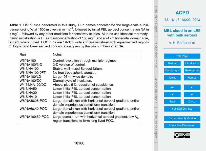
http://dx.doi.org/10.1016/j.atmosenv.2004.05.042

ACPD13, 18143–18203, 2013


A. H. Berner et al.

Title Page



Tables Figures

J I

J I

Back Close

Full Screen / Esc



Discussion

Paper

|D

iscussionP

aper|

Discussion

Paper

|D

iscussionP

aper|

Table 1. List of runs performed in this study. Run names concatenate the large-scale subsi-dence forcing W at 1500 m given in mm s−1, followed by initial PBL aerosol concentration NA in# mg−1, followed by any other modifiers for sensitivity studies. All runs use identical thermody-namic initialization, a FT aerosol concentration of 100 mg−1 and a 24 km horizontal domain size,except where noted. POC runs are 192 km wide and are initialized with equally-sized regionsof higher and lower aerosol concentration given by the two numbers after NA.

Run Notes

W5/NA100 Control; evolution through multiple regimes.W5/NA100/3-D 3-D version of control.W6.5/NA100 Stable, well mixed Sc equilibrium.W6.5/NA100-0FT No free tropospheric aerosol.W5/NA100/LD Larger 96 km wide domain.W5/NA100/DC Diurnal cycle of insolation.W4.75/NA100/DC Above, plus 5 % reduction of subsidence.W6.5/NA50 Lower initial PBL aerosol concentration.W6.5/NA30 Lower initial PBL aerosol concentration.W6.5/NA10 Lower initial PBL aerosol concentration.W5/NA30:25-POC Large domain run with horizontal aerosol gradient, entire

domain experiences cumuliform transition.W5/NA60:40-POC Large domain run with horizontal aerosol gradient, entire

domain experiences cumuliform transition.W5/NA100:50-POC Large domain run with horizontal aerosol gradient, low Na

region transitions to form long-lived POC.

18186





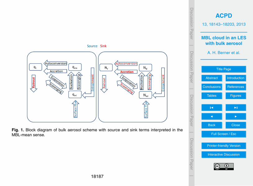
ACPD13, 18143–18203, 2013


A. H. Berner et al.

Title Page



Tables Figures

J I

J I

Back Close

Full Screen / Esc



Discussion

Paper

|D

iscussionP

aper|

Discussion

Paper

|D

iscussionP

aper|

Fig. 1. Block diagram of bulk aerosol scheme with source and sink terms interpreted in theMBL-mean sense.

18187





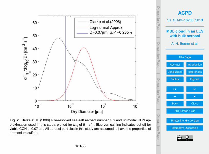
ACPD13, 18143–18203, 2013


A. H. Berner et al.

Title Page



Tables Figures

J I

J I

Back Close

Full Screen / Esc



Discussion

Paper

|D

iscussionP

aper|

Discussion

Paper

|D

iscussionP

aper|

Fig. 2. Clarke et al. (2006) size-resolved sea-salt aerosol number flux and unimodal CCN ap-proximation used in this study, plotted for u10 of 9 ms−1. Blue vertical line indicates cut-off forviable CCN at 0.07 µm. All aerosol particles in this study are assumed to have the properties ofammonium sulfate.

18188





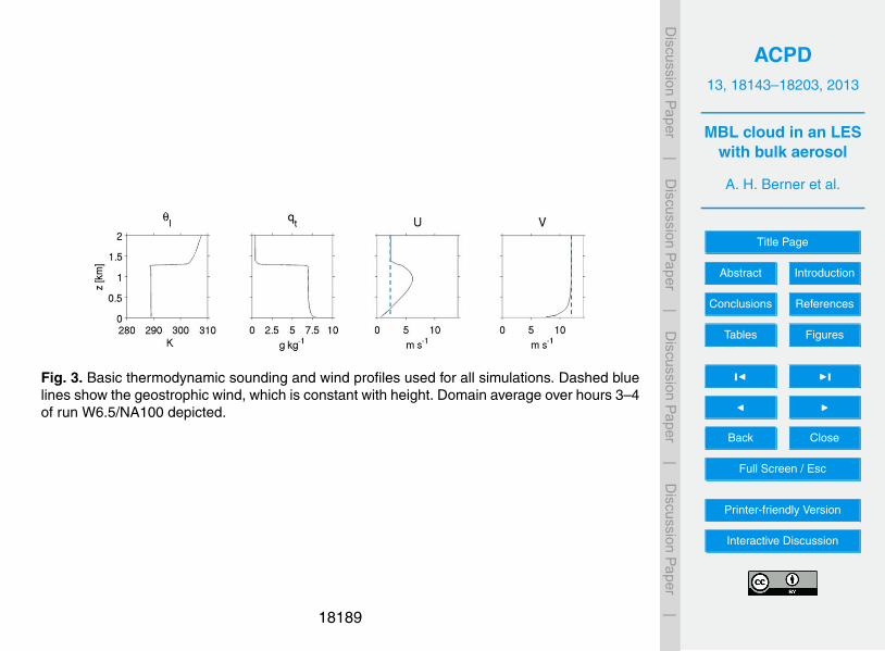
ACPD13, 18143–18203, 2013


A. H. Berner et al.

Title Page



Tables Figures

J I

J I

Back Close

Full Screen / Esc



Discussion

Paper

|D

iscussionP

aper|

Discussion

Paper

|D

iscussionP

aper|

Fig. 3. Basic thermodynamic sounding and wind profiles used for all simulations. Dashed bluelines show the geostrophic wind, which is constant with height. Domain average over hours 3–4of run W6.5/NA100 depicted.

18189





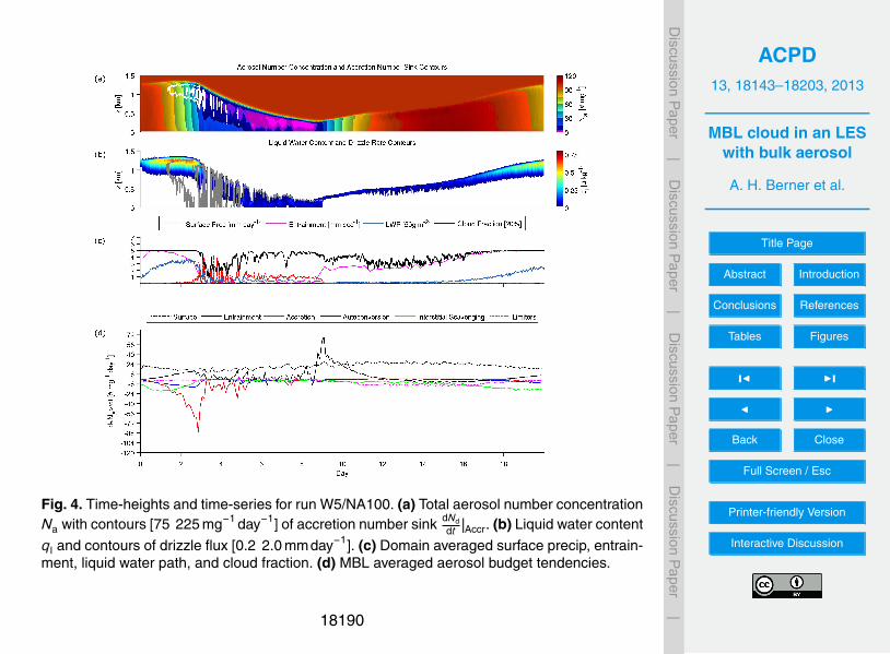
ACPD13, 18143–18203, 2013


A. H. Berner et al.

Title Page



Tables Figures

J I

J I

Back Close

Full Screen / Esc



Discussion

Paper

|D

iscussionP

aper|

Discussion

Paper

|D

iscussionP

aper|

Fig. 4. Time-heights and time-series for run W5/NA100. (a) Total aerosol number concentrationNa with contours [75 225 mg−1 day−1] of accretion number sink dNd

dt |Accr. (b) Liquid water content

ql and contours of drizzle flux [0.2 2.0 mmday−1]. (c) Domain averaged surface precip, entrain-ment, liquid water path, and cloud fraction. (d) MBL averaged aerosol budget tendencies.

18190





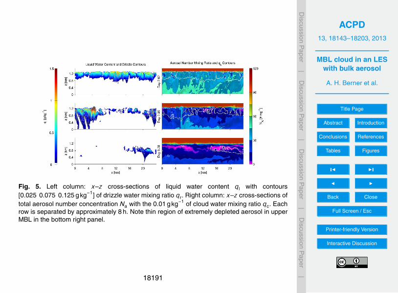
ACPD13, 18143–18203, 2013


A. H. Berner et al.

Title Page



Tables Figures

J I

J I

Back Close

Full Screen / Esc



Discussion

Paper

|D

iscussionP

aper|

Discussion

Paper

|D

iscussionP

aper|

Fig. 5. Left column: x–z cross-sections of liquid water content ql with contours[0.025 0.075 0.125 gkg−1] of drizzle water mixing ratio qr. Right column: x–z cross-sections oftotal aerosol number concentration Na with the 0.01 gkg−1 of cloud water mixing ratio qc. Eachrow is separated by approximately 8 h. Note thin region of extremely depleted aerosol in upperMBL in the bottom right panel.

18191





ACPD13, 18143–18203, 2013


A. H. Berner et al.

Title Page



Tables Figures

J I

J I

Back Close

Full Screen / Esc



Discussion

Paper

|D

iscussionP

aper|

Discussion

Paper

|D

iscussionP

aper|

Fig. 6. Comparison of two day period centered on transition in runs W5/NA100 (left) andW5/NA100/3-D (right). Rows as in panels a, b, and d of Fig. 4.

18192





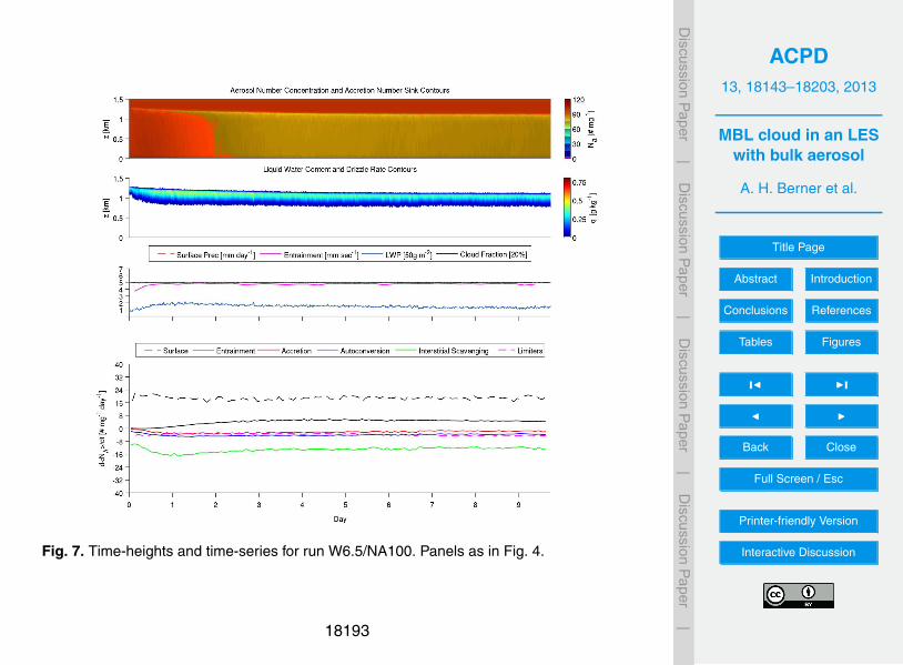
ACPD13, 18143–18203, 2013


A. H. Berner et al.

Title Page



Tables Figures

J I

J I

Back Close

Full Screen / Esc



Discussion

Paper

|D

iscussionP

aper|

Discussion

Paper

|D

iscussionP

aper|

Fig. 7. Time-heights and time-series for run W6.5/NA100. Panels as in Fig. 4.

18193





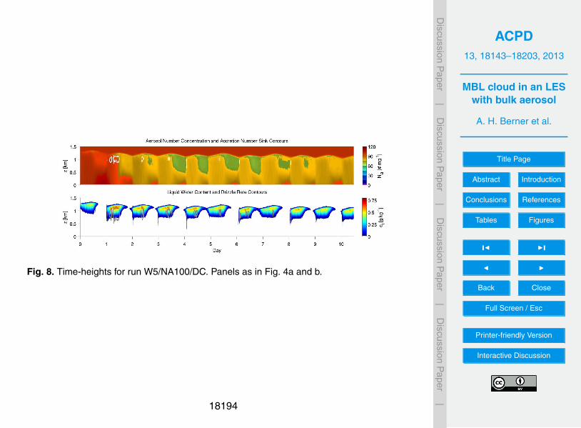
ACPD13, 18143–18203, 2013


A. H. Berner et al.

Title Page



Tables Figures

J I

J I

Back Close

Full Screen / Esc



Discussion

Paper

|D

iscussionP

aper|

Discussion

Paper

|D

iscussionP

aper|

Fig. 8. Time-heights for run W5/NA100/DC. Panels as in Fig. 4a and b.

18194





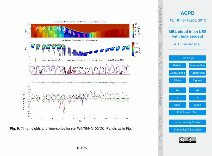
ACPD13, 18143–18203, 2013


A. H. Berner et al.

Title Page



Tables Figures

J I

J I

Back Close

Full Screen / Esc



Discussion

Paper

|D

iscussionP

aper|

Discussion

Paper

|D

iscussionP

aper|

Fig. 9. Time-heights and time-series for run W4.75/NA100/DC. Panels as in Fig. 4.

18195





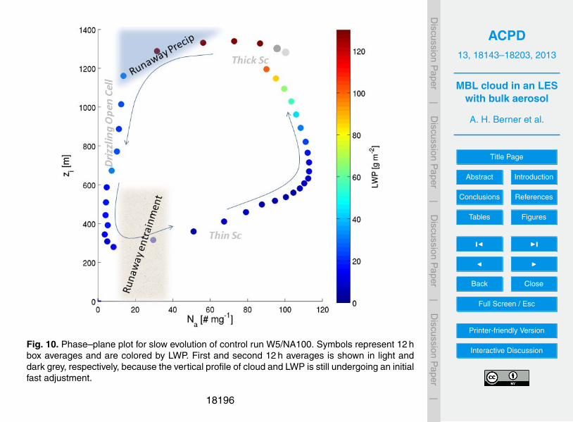
ACPD13, 18143–18203, 2013


A. H. Berner et al.

Title Page



Tables Figures

J I

J I

Back Close

Full Screen / Esc



Discussion

Paper

|D

iscussionP

aper|

Discussion

Paper

|D

iscussionP

aper|

Fig. 10. Phase–plane plot for slow evolution of control run W5/NA100. Symbols represent 12 hbox averages and are colored by LWP. First and second 12 h averages is shown in light anddark grey, respectively, because the vertical profile of cloud and LWP is still undergoing an initialfast adjustment.

18196





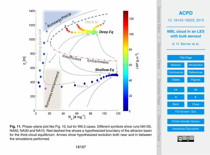
ACPD13, 18143–18203, 2013


A. H. Berner et al.

Title Page



Tables Figures

J I

J I

Back Close

Full Screen / Esc



Discussion

Paper

|D

iscussionP

aper|

Discussion

Paper

|D

iscussionP

aper|

Fig. 11. Phase–plane plot like Fig. 10, but for W6.5 cases. Different symbols show runs NA100,NA50, NA30 and NA10. Red dashed line shows a hypothesized boundary of the attractor basinfor the thick-cloud equilibrium. Arrows show hypothesized evolution both near and in betweenthe simulations performed.

18197





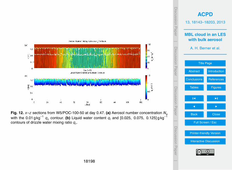
ACPD13, 18143–18203, 2013


A. H. Berner et al.

Title Page



Tables Figures

J I

J I

Back Close

Full Screen / Esc



Discussion

Paper

|D

iscussionP

aper|

Discussion

Paper

|D

iscussionP

aper|

Fig. 12. x–z sections from W5/POC-100-50 at day 0.47. (a) Aerosol number concentration Na

with the 0.01 gkg−1 qc contour. (b) Liquid water content ql and [0.025, 0.075, 0.125] g kg−1

contours of drizzle water mixing ratio qr.

18198





ACPD13, 18143–18203, 2013


A. H. Berner et al.

Title Page



Tables Figures

J I

J I

Back Close

Full Screen / Esc



Discussion

Paper

|D

iscussionP

aper|

Discussion

Paper

|D

iscussionP

aper|

Fig. 13. x–z sections from W5/POC-100-50 approximately 17.5 h later at day 1.21. Panels asin Fig. 12. Note the sharpened overall gradient and depletion of Na in the upper MBL within thePOC.

18199





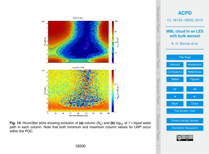
ACPD13, 18143–18203, 2013


A. H. Berner et al.

Title Page



Tables Figures

J I

J I

Back Close

Full Screen / Esc



Discussion

Paper

|D

iscussionP

aper|

Discussion

Paper

|D

iscussionP

aper|

Fig. 14. Hovmöller plots showing evolution of (a) column 〈Na〉 and (b) log10 of 1+ liquid waterpath in each column. Note that both minimum and maximum column values for LWP occurwithin the POC.

18200





ACPD13, 18143–18203, 2013


A. H. Berner et al.

Title Page



Tables Figures

J I

J I

Back Close

Full Screen / Esc



Discussion

Paper

|D

iscussionP

aper|

Discussion

Paper

|D

iscussionP

aper|

Fig. 15. Time-series averaged from 24 km wide strips centered within the overcast and POC.Left column shows panels (a) aerosol number concentration 〈Na〉, (b) inversion height zi, and(c) overcast fraction and domain-mean entrainment we; right column shows panels (d) LWPand CWP, (e) surface precipitation, and (f) cloud fraction.

18201





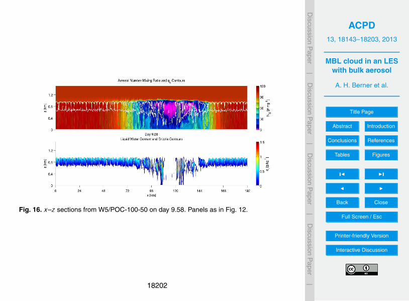
ACPD13, 18143–18203, 2013


A. H. Berner et al.

Title Page



Tables Figures

J I

J I

Back Close

Full Screen / Esc



Discussion

Paper

|D

iscussionP

aper|

Discussion

Paper

|D

iscussionP

aper|

Fig. 16. x–z sections from W5/POC-100-50 on day 9.58. Panels as in Fig. 12.

18202





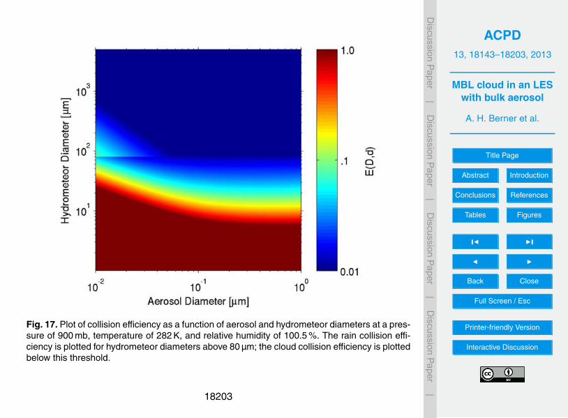
ACPD13, 18143–18203, 2013


A. H. Berner et al.

Title Page



Tables Figures

J I

J I

Back Close

Full Screen / Esc



Discussion

Paper

|D

iscussionP

aper|

Discussion

Paper

|D

iscussionP

aper|

Fig. 17. Plot of collision efficiency as a function of aerosol and hydrometeor diameters at a pres-sure of 900 mb, temperature of 282 K, and relative humidity of 100.5 %. The rain collision effi-ciency is plotted for hydrometeor diameters above 80 µm; the cloud collision efficiency is plottedbelow this threshold.

18203





MBL cloud in an LES with bulk aerosol

Documents

Transcript of MBL cloud in an LES with bulk aerosol