Cloud condensation nuclei prediction error from application of

Kohler theory: Importance for the aerosol indirect effect

Rafaella-Eleni P. Sotiropoulou,1 Athanasios Nenes,2 Peter J. Adams,3

and John H. Seinfeld4

Received 25 July 2006; revised 6 December 2006; accepted 27 February 2007; published 19 June 2007.

[1] In situ observations of aerosol and cloud condensation nuclei (CCN) and the GISSGCM Model II’ with an online aerosol simulation and explicit aerosol-cloud interactionsare used to quantify the uncertainty in radiative forcing and autoconversion rate fromapplication of Kohler theory. Simulations suggest that application of Kohler theoryintroduces a 10–20% uncertainty in global average indirect forcing and 2–11%uncertainty in autoconversion. Regionally, the uncertainty in indirect forcing rangesbetween 10–20%, and 5–50% for autoconversion. These results are insensitive to therange of updraft velocity and water vapor uptake coefficient considered. This studysuggests that Kohler theory (as implemented in climate models) is not a significant sourceof uncertainty for aerosol indirect forcing but can be substantial for assessments of aerosoleffects on the hydrological cycle in climatically sensitive regions of the globe. Thisimplies that improvements in the representation of GCM subgrid processes and aerosolsize distribution will mostly benefit indirect forcing assessments. Predictions ofautoconversion, by nature, will be subject to considerable uncertainty; its reduction mayrequire explicit representation of size-resolved aerosol composition and mixing state.

Citation: Sotiropoulou, R.-E. P., A. Nenes, P. J. Adams, and J. H. Seinfeld (2007), Cloud condensation nuclei prediction error from

application of Kohler theory: Importance for the aerosol indirect effect, J. Geophys. Res., 112, D12202, doi:10.1029/2006JD007834.

1. Introduction

[2] The Intergovernmental Panel on Climate Change[2001] identified indirect aerosol forcing as one of thelargest source of uncertainty in anthropogenic climateforcing, and urged the accurate representation of physico-chemical processes linking aerosols and clouds in globalmodels. Physically based approaches [Abdul-Razzak et al.,1998; Cohard et al., 1998; Abdul-Razzak and Ghan, 2000;Cohard et al., 2000; Nenes and Seinfeld, 2003; Fountoukisand Nenes, 2005] rely on theory first introduced by Kohler[1921], in which aerosol is assumed to be composed of amixture of deliquescent electrolytes and insoluble material.Subsequent modifications to Kohler theory consider morecomplex aerosol-water interactions, such as the presence ofslightly soluble compounds [e.g., Shulman et al., 1996],surfactants [Shulman et al., 1996; Facchini et al., 1999],black carbon inclusions [Conant et al., 2002], soluble

gases [Kulmala et al., 1993], and solute dissolution kinetics[Asa-Awuku and Nenes, 2007].[3] Assessing the applicability of Kohler theory (and its

extensions) is required for improving predictions of aerosol-cloud interactions. The ultimate test is CCN ‘‘closure,’’ orcomparing predictions of CCN concentrations (from appli-cation of Kohler theory to measurements of size distributionand chemical composition) with measurements obtainedwith a CCN counter. A multitude of CCN closure studieshave been carried out with varying degrees of success, withprediction errors usually within 10–50% [e.g., Medina etal., 2007, and references therein]. In situ cloud drop numberconcentration (CDNC) closure studies [e.g., Conant et al.,2004; Meskhidze et al., 2005; Fountoukis et al., 2007] arealso a good test of Kohler theory, although the degree ofclosure depends on the accuracy of other measured param-eters, such as droplet concentration and cloud updraftvelocity.[4] Closure studies typically focus on CCN prediction

error, but do not relate it to uncertainty in the aerosolindirect effect; the latter remains an outstanding issue forconstraining anthropogenic climate forcing. Sotiropoulou etal. [2006] first addressed this problem; using ground-basedCCN and aerosol measurements in combination with theFountoukis and Nenes [2005] cloud droplet formationparameterization, CDNC uncertainty resulting from appli-cation of Kohler theory was found to be roughly half theCCN prediction uncertainty for a wide range of aerosolconcentration, updraft velocity and droplet growth kinetics.This study extends the analysis of Sotiropoulou et al.

JOURNAL OF GEOPHYSICAL RESEARCH, VOL. 112, D12202, doi:10.1029/2006JD007834, 2007ClickHere

for

FullArticle

1School of Earth and Atmospheric Sciences, Georgia Institute ofTechnology, Atlanta, Georgia, USA.

2Schools of Earth and Atmospheric Sciences and Chemical andBiomolecular Engineering, Georgia Institute of Technology, Atlanta,Georgia, USA.

3Departments of Civil and Environmental Engineering and Engineeringand Public Policy, Carnegie Mellon University, Pittsburgh, Pennsylvania,USA.

4Departments of Chemical Engineering and Environmental Science andEngineering, California Institute of Technology, Pasadena, California, USA.

Copyright 2007 by the American Geophysical Union.0148-0227/07/2006JD007834$09.00

D12202 1 of 12

[2006], and uses a global model to assess the uncertainty incloud droplet number, indirect radiative forcing (i.e., ‘‘first’’aerosol indirect effect) and autoconversion associated withapplication of Kohler theory. Hereon, the term ‘‘CCNprediction error’’ expresses the error arising from applica-tion of Kohler theory. CCN uncertainty associated witherrors in predicted aerosol size distribution and chemicalcomposition are left for a future study.

2. Description of Global Model

[5] The 9-layer NASA Goddard Institute for Space Stud-ies (GISS) general circulation model (GCM) Model II’[Hansen et al., 1983; Del Genio et al., 1996] with 4� �5� horizontal resolution and nine vertical layers (fromsurface to 10 mbar) is used. The model simulates theemissions, transport, chemical transformation and deposi-tion of chemical tracers such as sulfate (SO4

2�), ammonium(NH4

+), dimethyl sulfide (DMS), methanesulfonic acid(MSA), sulfur dioxide (SO2), ammonia (NH3), and hydro-gen peroxide (H2O2). The model time step for theseprocesses is one hour. A quadratic upstream module foradvection of heat and moisture and a fourth-order schemefor tracer advection are used [Del Genio et al., 1996]. Seasurface temperatures are climatologically prescribed.[6] Moist convection is implemented by a mass flux

scheme that considers entraining and nonentraining plumes,compensating subsidence and downdrafts [Del Genio andYao, 1993]. Liquid water associated with convective cloudseither precipitates, evaporates or detrains into the large-scalecloud cover within the model time step. Liquid water iscarried as a prognostic variable in the large-scale cloudscheme [Del Genio et al., 1996], allowing large-scale cloudsto persist for several time steps.[7] The parameterization of cloud formation follows the

approach of Sundqvist et al. [1989], in which the grid cloudfraction is proportional to the difference between the aver-age grid box relative humidity and the relative humidity inthe clear fraction of the grid [Del Genio et al., 1996].Autoconversion of cloud water to precipitation is parame-terized as [Del Genio et al., 1996],

_qlð ÞAU¼ C0ql 1� exp � qc

qcrit

� �4" #( )

ð1Þ

where ( _ql)AU is the autoconversion rate (s�1), qcrit is thecritical cloud water content for the onset of rapid conversion(g m�3), C0 is the limiting autoconversion rate (s�1), qc isthe in-cloud liquid water content (g m�3) and ql is the liquidwater mixing ratio.[8] The GISS radiative scheme [Hansen et al., 1983]

computes the absorption and scattering of radiation by gasesand particles. The gaseous absorbers included in the GCMare H2O, CO2, O3, O2, and NO2, utilizing twelve spectrallynoncontiguous, vertically correlated-k distribution intervals.Cloud and aerosol radiative parameters (extinction crosssection, single scattering albedo, and asymmetry parameter)are treated using radiative properties obtained from Miecalculations for the global aerosol climatology of Toon andPollack [1976]. Six intervals for the spectral dependence ofMie parameters for clouds, aerosol and Rayleigh scattering

are used [Hansen et al., 1983]. Multiple scattering of solarradiation utilizes the doubling/adding method [Lacis andHansen, 1974] with single Gauss point adaptation to repro-duce the solar zenith angle dependence for reflected solarradiation by clouds and aerosols with the same degree ofprecision as the full doubling-adding for conservative scat-tering. The six spectral intervals are superimposed withtwelve absorption coefficient profiles to account for over-lapping absorption.

2.1. Online Aerosol Simulation

[9] Anthropogenic emissions include the seasonal emis-sions of SO2 from fossil fuel combustion, industrial activ-ities [Baughcum et al., 1993; Benkovitz et al., 1996] andbiomass burning [Spiro et al., 1992] compiled by the GlobalEmission Inventory Activity (GEIA) [Guenther et al.,1995]. Natural emissions include SO2 from noneruptivevolcanoes [Spiro et al., 1992] and oceanic DMS [Liss andMerlivat, 1986; Kettle et al., 1999]. Anthropogenic andnatural emissions of NH3 from domestic animals, fertilizers,soils and crops, oceans, biomass burning and humans arealso considered [Bouwman et al., 1997].[10] Global aerosol mass concentrations are simulated

online [Adams et al., 1999, 2001; Koch et al., 1999].Aerosol is internally mixed, composed of sulfate (SO4

2�),ammonium (NH4

+), nitrate (NO3�), methanesulfonic acid

(MSA) and water. Gas phase species simulated are dimethylsulfide (DMS), sulfur dioxide (SO2), ammonia (NH3) andhydrogen peroxide (H2O2). Gas phase reactions consideredare of DMS with hydroxyl (OH) and nitrate (NO3) radicalsand oxidation of SO2 by OH. In-cloud formation of SO4

2�

from the oxidation of HSO3� by H2O2 is also considered.

Volatile inorganic species (NH4+, NO3

�, H2O) are assumed tobe in thermodynamic equilibrium over the 1-hour modeltime step [Adams et al., 1999]; ISORROPIA [Nenes et al.,1998, 1999] determines the partitioning of the volatilechemical species, ammonia, nitrate and water between thegas and the aerosol phase based on the temperature, relativehumidity and amount of aerosol precursor in each grid cell.[11] The aerosol simulation has been extensively evalu-

ated with a wide variety of observations [Adams et al.,1999; Koch et al., 1999]. Simulated concentrations ofsulfate and ammonium generally agree within a factor oftwo with EMEFS and EMEP observations. Annual averagenitrate concentrations are not reproduced as well, likelyfrom uncertainties in measurements in aerosol nitrate [Yu etal., 2005], to uncertainty in predicted ammonium andsulfate (which control aerosol pH, hence nitrate partition-ing) and interaction of HNO3 with dust and sea salt.

2.2. Aerosol-Cloud Interactions

[12] Aerosol microphysical parameters for CDNC calcu-lations are obtained by scaling prescribed aerosol sizedistributions to the simulated online sulfate mass concen-tration (section 2.1); aerosol nitrate is subject to consider-able error and therefore is not considered. Two types ofaerosol size distributions are prescribed: (1) marine, for gridcells over the ocean, and, (2) continental, for grid cells overland (Table 1). Both aerosol types are assumed to be amixture of ammonium sulfate and insoluble material.[13] CDNC is computed using the physically based

parameterization of Fountoukis and Nenes [2005]. This

D12202 SOTIROPOULOU ET AL.: AEROSOL INDIRECT EFFECT UNCERTAINTY

2 of 12

D12202

parameterization is one of the most comprehensive andcomputationally efficient formulations available for globalmodels. Its accuracy has been evaluated with detailednumerical simulations [Nenes and Seinfeld, 2003;Fountoukisand Nenes, 2005] and in situ data for cumuliform andstratiform clouds of marine and continental origin[Meskhidze et al., 2005; Fountoukis et al., 2007]. Theparameterization is based on the framework of an ascendingcloud parcel; the maximum supersaturation, smax, controlsCDNC and is determined by the balance of water vaporavailability from cooling and depletion from the condensa-tional growth of activated droplets. The concept of ‘‘popu-lation splitting’’ (in which droplets are classified by theproximity to their critical diameter) allows smax to bedetermined from the numerical solution of an algebraicequation. Population splitting also allows the accuratetreatment of complex aerosol chemistry and kinetic limi-tations on droplet growth, such as from the presence oforganics that depress surface tension and water vaporuptake [e.g., Fountoukis and Nenes, 2005].[14] In our simulations, a single cloud-base updraft ve-

locity is prescribed to compute droplet number, which forthe ‘‘base case’’ simulation is set to 1 m s�1 over land and0.5 m s�1 over ocean. The ‘‘base case’’ value of water vapormass uptake coefficient, ac, is set to 0.042, consistent withlaboratory [Pruppacher and Klett, 1997; Shaw and Lamb,1999], and in situ CDNC closure studies [Conant et al.,2004; Meskhidze et al., 2005; Fountoukis et al., 2007]. Thesensitivity of our simulations to the updraft velocity and ac

is also considered (section 6).

3. Quantification of CCN Prediction Error

[15] In situ measurements of aerosol size distribution,chemical composition and CCN concentrations are usedfor characterizing CCN prediction error. The data wasobtained at the Atmospheric Investigation, Regional Mod-eling, Analysis and Prediction (AIRMAP) Thompson Farm(TF) site (Durham, NH) during the ICARTT (InternationalConsortium for Atmospheric Research on Transport andTransformation) campaign (July–August 2004). TF aerosolis primarily regional, influenced by some local biogenicemissions from the surrounding forest [e.g., DeBell et al.,2004].[16] CCN concentrations were measured at 0.20, 0.30,

0.37, 0.50, and 0.60% s, with a Droplet MeasurementTechnologies, Inc. (DMT) streamwise thermal gradientcloud condensation nuclei counter [Roberts and Nenes,2005; Lance et al., 2006]. Throughout the measurementperiod, the CCN counter operated at a flow rate of 0.5 Lmin�1 with a sheath-to-aerosol flow ratio of 10:1. CCNconcentrations were measured at each s for 6 minutes

yielding a spectrum every 30 minutes. Measurements ofthe aerosol size distribution were obtained every twominutes for mobility diameters between 7 and 289 nm witha TSI Scanning Mobility Particle Sizer (SMPS, model 3080,which included a TSI model 3010 Condensation ParticleCounter (CPC) and a TSI model 3081L long DifferentialMobility Analyzer (DMA)). Simultaneously, size-resolvedchemical composition was measured every 10 minutes withan Aerodyne Aerosol Mass Spectrometer (AMS) [Jayne etal., 2000].[17] For most of the period, polluted continental air was

sampled from the Great Lakes; roughly equal amounts offreshly condensed secondary organic aerosols (SOA) andprimary organic carbon (POA) composed the carbonaceousfraction (L. D. Cottrell et al., Submicron particles atThompson Farm during ICARTT measured using aerosolmass spectrometry, manuscript in preparation, 2007, here-inafter referred to as Cottrell et al., manuscript in prepara-tion, 2007). Occasionally, polluted rural air (characterizedby higher CCN concentrations and larger sulfate massfractions) was collected from south of the sampling site.The sulfate mass fraction ranged in our data set between0.06 and 0.54, with an average of 0.24 ± 0.09. Sulfate andammonium always dominated the inorganic fraction. Theaerosol number concentration ranged between 1366 and8419 cm�3 with an average of 3786 ± 1360 cm�3. Adetailed description and analysis of the data set is givenby Medina et al. [2007] and Cottrell et al. (manuscript inpreparation, 2007).[18] Kohler theory, combined with the observed aerosol

size distribution and chemical composition from theICARTT campaign yields ‘‘predicted’’ CCN concentrations.Following Sotiropoulou et al. [2006], both ‘‘predicted’’ and‘‘observed’’ CCN concentrations are fit to the ‘‘modifiedpower law’’ form of Cohard et al. [1998, 2000], whereCCN approach a constant value at high supersaturations(which in this study is taken to be the total aerosol number).The ‘‘modified power law’’ is selected for its simplicity, andability to describe a CCN spectrum for a very wide range ofsupersaturations [Cohard et al., 1998, 2000].[19] The degree of CCN closure is typical of polluted

environments and larger than for pristine ones [Medina etal., 2007, and references therein]; using size-averagedchemical composition, CCN closure is achieved within36 ± 29%, while introducing size-dependent chemicalcomposition CCN concentrations is overpredicted by 17 ±27%. Under certain conditions (e.g., externally mixedaerosol or freshly emitted carbonaceous aerosol) the closureerror may be larger; whether or not this is important enoughto have a global impact remains to be seen. For this study,

Table 1. Trimodal Lognormal Aerosol Size Distributions Used in This Studya

Aerosol Type

Nuclei Mode Accumulation Mode Coarse Mode

Dg s Nap cSO4 Dg s Nap cSO4 Dg s Nap cSO4

Marine 0.020 1.47 230 0.33 0.092 1.60 177 0.33 0.580 2.49 3.10 0.95Continental 0.016 1.60 1000 0.50 0.067 2.10 800 0.50 0.930 2.20 0.72 0.50

aDg is the modal geometric mean diameter (mm), Nap is the mode concentration (cm�3), s is the geometric standard deviation, and cSO4 is the sulfatemass fraction. Distributions obtained from Whitby [1978].

D12202 SOTIROPOULOU ET AL.: AEROSOL INDIRECT EFFECT UNCERTAINTY

3 of 12

D12202

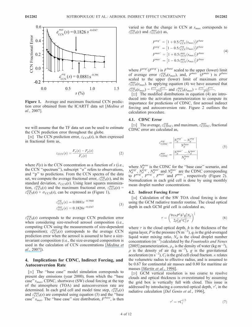
we will assume that the TF data set can be used to estimatethe CCN prediction error throughout the globe.[20] The CCN prediction error, eCCN(s), is then expressed

in fractional form as,

eCCN sð Þ ¼ Fo sð Þ � Fp sð ÞFo sð Þ ð2Þ

where F(s) is the CCN concentration as a function of s (i.e.,the CCN ‘‘spectrum’’), subscript ‘‘o’’ refers to observations,and ‘‘p’’ to predictions. From the CCN spectra of the dataset, we compute the average fractional error, eCCN

avg (s), and itsstandard deviation, sCCN(s). Using least squares minimiza-tion, eCCN

avg (s) and the maximum fractional error, eCCNmax (s) =

eCCNavg (s) + sCCN(s), can be expressed as (Figure 1),

eavgCCN sð Þ ¼ 0:0881s�0:3960

emaxCCN sð Þ ¼ 0:1826s�0:4347 ð3Þ

eCCNavg (s) corresponds to the average CCN prediction errorwhen considering size-resolved aerosol composition (i.e.,computing CCN using the measurements of size-dependentcomposition); eCCN

max (s) corresponds to the average CCNprediction error when the aerosol is assumed to have a size-invariant composition (i.e., the size-averaged composition isused in the calculation of CCN concentrations [Medina etal., 2007]).

4. Implications for CDNC, Indirect Forcing, andAutoconversion Rate

[21] The ‘‘base case’’ model simulation corresponds topresent day emissions (year 2000), from which the ‘‘basecase’’ smax, CDNC, shortwave (SW) cloud forcing at the topof the atmosphere (TOA) and autoconversion rate aredetermined. In each grid cell and model time step, eCCN

avg (s)and eCCN

max (s) are computed using equation (3) and the ‘‘basecase’’ smax. The ‘‘base case’’ size distribution, F

base, is then

varied so that the change in CCN at smax corresponds toeCCNavg (s) and eCCN

max (s) as,

Favgþ ¼ 1þ 0:5eavgCCN smaxð Þ� �

Fbase

Favg� ¼ 1� 0:5eavgCCN smaxð Þ� �

Fbase

Fmaxþ ¼ 1þ 0:5emaxCCN smaxð Þ� �

Fbase

Fmax� ¼ 1� 0:5emaxCCN smaxð Þ� �

Fbase ð4Þ

where Favg+(Favg�) is Fbase scaled to the upper (lower) limitof average error eCCN

avg (smax), and, Fmax+ (Fmax�) is Fbase

scaled to the upper (lower) limit of maximum erroreCCNmax (smax). In applying equation (4) we have assumed that

eCCNavg (smax) =

Favgþ�Favg�

Fbase and eCCNmax (smax) =

Favgþ�Favg�

Fbase .[22] The modified distributions in equation (4) are intro-

duced into the activation parameterization to compute itsimportance for predictions of CDNC, first aerosol indirectforcing and autoconversion rate. Figure 2 outlines thecalculation procedure.

4.1. CDNC Error

[23] The average, eCDNCavg , and maximum, eCDNC

max , fractionalCDNC error are calculated as,

eavgCDNC ¼ Navgþ

d � Navg�

d

Nbased

emaxCDNC ¼ Nmaxþ

d � Nmax�

d

Nbased

ð5Þ

where Ndbase is the CDNC for the ‘‘base case’’ scenario, and

Ndavg+, Nd

avg�, Ndmax+ and Nd

max� are the CDNC correspondingto Favg+, Favg�, Fmax+ and Fmax�, respectively (Figure 2).Normalization in each grid cell is done by using monthlymean droplet number concentrations.

4.2. Indirect Forcing Error

[24] Calculation of the SW TOA cloud forcing is doneusing the GCM radiative transfer routine. The cloud opticaldepth in each GCM grid cell is calculated as,

t ¼ 9pkP3h3q2l Nd

2r2wg3C2l r

� �13

ð6Þ

where t is the cloud optical depth, h is the thickness of thesigma layer, P is the pressure (N m�2), ql is the grid-averagedliquid water mixing ratio, Nd is the cloud droplet numberconcentration (m�3) calculated by the Fountoukis and Nenes[2005] parameterization, rw is the density of water (kg m�3),r is the density of air (kg m�3), g is the gravitationalacceleration (m s�2),Cl is the grid cell cloud fraction. k relatesthe volumetric radius to effective radius, and is assumed tobe 0.67 for continental air masses and 0.80 for maritime airmasses [Martin et al., 1994].[25] GCM vertical resolution is too coarse to resolve

clouds and optical thickness is overestimated by assumingthe grid box is vertically full with cloud. This issue isaddressed by introducing a corrected optical depth, t0, in theradiative calculation [Del Genio et al., 1996],

t0 ¼ tC1=3l ð7Þ

Figure 1. Average and maximum fractional CCN predic-tion error obtained from the ICARTT data set [Medina etal., 2007].

ð4Þ

ð3Þ

ð5Þ

D12202 SOTIROPOULOU ET AL.: AEROSOL INDIRECT EFFECT UNCERTAINTY

4 of 12

D12202

[26] The average, UIFavg, and maximum, UIF

max, error inindirect forcing arising from CCN prediction error is,

UavgIF ¼ CF

avgþ

TOA � CFavg�

TOA

Umax

IF ¼ CFmaxþ

TOA � CFmax�

TOA

ð8Þ

where CFTOAavg+, CFTOA

avg�, CFTOAmax+, and CFTOA

max� are the SWTOA cloud forcings for optical depths corresponding toF avg+, F avg�, F max+ and F max�, respectively.

4.3. Impact on Autoconversion Rate

[27] Results are expressed in terms of the average, UavgAU,

and maximum, U maxAU, fractional error in autoconversion

rate,

UavgAU ¼ _qlð Þavg

þ

AU � _qlð Þavg�

AU

_qlð ÞbaseAU

UmaxAU ¼ _qlð Þmax

þ

AU � _qlð Þmax�

AU

_qlð ÞbaseAU

ð9Þ

where ( _ql)AUbase is the ‘‘base case’’ autoconversion rate,

( _ql)AUavg+, ( _ql)AU

avg�, ( _ql)AUmax+ and ( _ql)AU

max� are the autoconversionscorresponding toF avg+,F avg�,F max+ andF max�, respectively.Normalization in each grid cell is done by using monthlymean autoconversion rates.

[28] Autoconversion rates vary substantially betweenparameterizations; to assess the robustness of our results,we repeat the error calculation for multiple autoconversionformulations. We use the parameterizations of Rotstayn[1997] and Khairoutdinov and Kogan [2000], which ex-plicitly consider CDNC. Rotstayn [1997] modified the workof Manton and Cotton [1977] to account for the fractionalcloudiness often encountered in a GCM grid cell,

_qlð ÞAU¼ �Cl

0:104gEAUr43

m Ndrwð Þ13

ql

Cl

� �73

Hql

Cl

� qCR

� �ð10Þ

where m is the dynamic viscosity of air (kg m�1 s�1), andEAU is the mean collection efficiency (assumed to be 0.55).H is the Heaviside function which suppresses autoconver-sion until

qlCl

reaches a ‘‘critical’’ liquid water mixing

ratio, qCR = 43prwrCR

3 Nd/r (where rCR is the ‘‘critical’’

volume-mean cloud droplet radius for the onset of auto-conversion, set to 7.5 mm).[29] Khairoutdinov and Kogan [2000] developed their

parameterizations using Large Eddy Simulations of strato-cumulus cloud fields. Two formulations are provided, oneexplicitly in terms of droplet number,

_qlð ÞAU¼ 1350Cl

ql

Cl

� �2:47

Nd � 10�6 ��1:79 ð11Þ

Figure 2. Methodology used for estimating the error in CCN, CDNC, indirect forcing andautoconversion rate.

ð8Þ

D12202 SOTIROPOULOU ET AL.: AEROSOL INDIRECT EFFECT UNCERTAINTY

5 of 12

D12202

and another, in terms of drop mean volume radius, rv (mm):

_qlð ÞAU¼ 4:1� 1015Clr5:67v ð12Þ

Equations (11) and (12) have been modified to account forthe fractional cloud cover in the GCM grid cell.[30] Equations (10), (11), and (12) consider changes in

autoconversion from increases in submicron CCN concen-trations, but not the impact of giant CCN (GCCN) ondrizzle formation. The latter have been shown to acceleratethe formation of drizzle in numerous remote sensing[Rosenfeld et al., 2002; Rudich et al., 2002] and modelingstudies [Levin et al., 1996; Reisin et al., 1996; Feingold etal., 1999; Yin et al., 2000; Zhang et al., 2006]. Despite theirpotential importance, including the impact of GCCN onautoconversion is challenging (and currently not consideredin parameterizations) because of the highly nonlinear phys-ics involved and the lack of observational constraints.GCCN impacts may not be as important in our study,because we are assessing autoconversion changes that arisefrom differences in aerosol chemical composition (more

exactly, its size dependence), but not size distribution. Shiftsin composition would not affect concentrations of GCCN inall of the simulations, as their large size (i.e., very lowcritical supersaturation) ensures that they would alwaysactivate, regardless of their composition. Thus GCCNimpacts on cloud microphysics will affect primarily the‘‘base case’’ value of autoconversion but not its sensitivityto modest changes in CCN concentrations. It should benoted however that our simulations do not completelyneglect the presence of GCCN; their impact on smax (bycompeting for water vapor) is considered, as our prescribedlognormal distributions predict nonnegligible concentra-tions of GCCN in most regions of the globe.

5. Results and Discussion

5.1. Base Case Simulation

[31] Figure 3 presents the ‘‘base case’’ annual meanCDNC (Figure 3, top) and preindustrial-current day aerosolindirect forcing (Figure 3, bottom). Largest values of CDNCare predicted in the midlatitudes of the Northern Hemi-sphere, downwind of sources in industrialized regions. Highvalues of CDNC are also seen in the North Atlantic, fromlong-range transport of pollution plumes, and in the South-ern Hemisphere downwind of biomass burning regions.Figure 3 also illustrates the annual mean anthropogenicaerosol indirect forcing (Figure 3, bottom), defined as thedifference in the TOA net shortwave incoming flux betweenthe present-day and preindustrial simulations. The globallyaveraged TOA indirect radiative forcing is �1.00 W m�2,consistent with most assessments to date [e.g., Suzuki et al.,2004; Lohmann and Feichter, 2005]. The spatial pattern ofindirect forcing tends to follow that of CDNC, with largestvalues (��10 W m�2) computed downwind of industrial-ized regions of the globe.

5.2. Fractional CCN Error

[32] The spatial distributions of eCCNavg and eCCN

max in themodel surface layer are presented in Figure 4. The globalaverage eCCN

avg (Figure 4a) is 0.09 (i.e., 9%), and the globalmean eCCN

max (Figure 4b) is 0.18 (i.e., 18%). Larger CCNprediction error is found where in-cloud smax is low, such asin regions affected by industrial pollution plumes (NorthAmerica, Europe) and long-range transport of pollutionplumes (North Atlantic). Between 20 and 60�N, the annualmean eCCN

avg (eCCNmax ) is 0.10 (0.21); for the continental United

States the corresponding values are 0.10 (0.22), and forEurope, 0.11 (0.24). In pristine areas, in-cloud smax is high(between 1% and 2%), suppressing CCN prediction error(which ranges between 0.09 and 0.15). The above analysissuggests that assuming internally mixed aerosols with asize-invariant chemical composition (expressed by eCCN

max )results in twice the CCN prediction error compared toassuming size-resolved chemical composition (expressedby eCCN

avg ). Variations in CCN concentration changes cloudsmax 0.04% between F avg+ and F avg�, and 0.08% betweenFmax+ and Fmax�.

5.3. Fractional CDNC Error

[33] Figure 4 presents eCDNCavg (Figure 4c) and eCDNC

max

(Figure 4d) that result from eCCNavg (Figure 4a) and eCCN

max

(Figure 4b), respectively. Since CCN changes generally

Figure 3. (top) ‘‘Base case’’ annual mean cloud dropletnumber concentrations (cm�3) and (bottom) anthropogenicaerosol indirect forcing (W m�2). The global average isshown in the upper right hand corner of each panel.

D12202 SOTIROPOULOU ET AL.: AEROSOL INDIRECT EFFECT UNCERTAINTY

6 of 12

D12202

lead to a sublinear response in CDNC, eCDNC is spatiallycorrelated with eCCN, but is of smaller magnitude. Largervalues of CDNC error are predicted over continents in theNorthern Hemisphere; between 20 and 60�N, eCDNC

avg is 0.08and eCDNC

max is 0.17. The same applies over Europe andthe continental US, while CDNC error over pristineregions tends to be smaller, ranging between 0.05 and0.15 (Figure 4). In summary, CCN prediction error impliesa 8–17% CDNC error in polluted regions, and a 5–15%error in pristine regions of the globe.

5.4. Relative Sensitivity of CDNC to CCN

[34] Dividing the fractional errors yields the relativesensitivity of CDNC to CCN error, F:

F ¼ eavgCCN smaxð ÞeavgCDNC

oremaxCCN smaxð ÞemaxCDNC

ð13Þ

[35] Low values of F suggest high sensitivity of CDNCto CCN prediction error and vice versa.[36] Figure 5 presents the spatial distribution of the

annual F. Smaller values of F are observed over pristineregions, where CCN and CDNC concentrations are low,hence CDNC are more sensitive to CCN prediction error.The highest F is predicted for polluted regions, such as SWUSA, Europe, and Asia. In such regions, the large error inpredicted CCN concentrations does not translate to largeerror in CDNC, because dynamical readjustment of in-cloudsmax under polluted conditions tends to compensate for

changes in CCN. The area NE of India (Tibetan plateau)has a F value close to unity, because CCN concentrationsare low and in-cloud smax is high. The annual average Fbetween 20 and 60�N is 1.22; for USA and Europe, Franges between 1.25 and 1.30. This means that CDNC erroris 22–30% lower than CCN prediction error for pollutedregions of the globe.

5.5. Impact of CCN Error on Cloud Radiative Forcing

[37] The spatial distributions of U avgIF , and Umax

IF areshown in Figures 6a and 6b, respectively. The average error

Figure 4. Annual average surface layer (a) eCCNavg , (b) eCCN

max , (c) eCDNCavg , and (d) eCDNC

max . The globalaverage value is shown in the upper right hand corner of each panel.

Figure 5. Annual mean F in the model surface layer. Theglobal average is shown in the upper right hand corner.

D12202 SOTIROPOULOU ET AL.: AEROSOL INDIRECT EFFECT UNCERTAINTY

7 of 12

D12202

in indirect forcing is equal to 0.1 W m�2 while thecorresponding maximum error is equal to 0.2 W m�2. ThusCCN prediction error leads to a 10–20% error in globalindirect effect. Regionally, indirect forcing error is highest(�0.5 W m�2) downwind of industrialized and biomassburning regions; SW forcing in the surface layer of theoceans is thus subject to a 5–20% error. The least indirectforcing error is predicted over deserts and the subtropicalsouthern oceans, where anthropogenic CCN perturbationsare least effective in affecting cloud optical depth.

5.6. Impact of CCN Error on Autoconversion Rate

[38] Autoconversion parameterizations are usually‘‘tuned’’ to reproduce observations; we did not follow thisprocedure to explore the robustness of UAU

avg and UAUmax, in the

absence of tuning. Figure 7 presents ‘‘base case’’ autocon-version rates for each parameterization considered in thisstudy (equations (1) and (10)–(12)). All parameteriza-tions are anticorrelated with the spatial patterns of CDNC(Figure 3), but differ substantially (a factor of 20) in predictedautoconversion rate. Compared to the ‘‘default’’ GISSautoconversion scheme (equation (1)), Khairoutdinov andKogan [2000] predicts lower autoconversion and Rotstayn’s[1997], higher (Figure 7). The difference between theparameterizations are not a result of error in predicted cloud

microphysical characteristics (droplet number concentration,liquid water content), but rather an inherent error in theparameterizations. Compared to the parameterization ofRotstayn [1997], the contrast between land and sea is largerusing Khairoutdinov and Kogan’s [2000] parameterization;this is not surprising, given the stronger dependence ofequation (11) on CDNC. The discrepancy between formu-lations could be reduced if the parameterizations are tunedto match observations; this is beyond the scope of thisstudy.[39] The average and maximum errors in autoconversion

rates using the schemes of Khairoutdinov and Kogan [2000]and Rotstayn [1997] are shown in Figure 8. The largestautoconversion error is predicted for polluted regions,because pristine clouds, contrary to their polluted counter-parts, have a high precipitation efficiency (since theirdroplets are generally large) hence are less sensitive toCDNC error. The autoconversion schemes of Khairoutdinovand Kogan [2000] are most sensitive to Nd, hence CDNCerror (Table 2). As a result, the percent UAU

avg (UAUmax) induced

by Kohler theory using equation (11) is 5.6% (11.4%),while the corresponding one using equation (10) is 2.3%(4.7%).

6. Sensitivity Tests

[40] It is instructive to explore the sensitivity of ourfindings to poorly constrained parameters that influencecloud droplet formation, namely, updraft velocity and ac.The sensitivity tests are done for conditions that woulddecrease in-cloud smax; simulations for higher smax are notrequired, as that would further decrease the already small‘‘base case’’ error in CDNC and indirect forcing.[41] It is well known that droplet number is a strong

function of updraft velocity, as it controls the parcelexpansion rate (i.e., cooling rate), hence parcel supersatu-ration, droplet concentration, size and the time available forcoalescence. At cloud base, a decrease in updraft velocitydecreases CDNC and vice versa (everything else beingequal). Since cloud-base updrafts are not explicitly resolvedin GCMs, but prescribed (as is done in this study) ordiagnosed from turbulent kinetic energy, it constitutes amajor source of error in CDNC calculations. We repeat the‘‘base case’’ simulation, but for updraft velocity equal to0.5 m s�1 over land and 0.25 m s�1 over ocean.[42] ac, formally defined as the probability of a water

vapor molecule remaining in the liquid phase upon collisionwith a droplet [Seinfeld and Pandis, 1998], is a parameterwhich determines the size dependence of the water vapormass transfer coefficient. Despite the considerable work todate [see Fountoukis and Nenes, 2005, and referencestherein], ac is still subject to substantial error [e.g.,Fountoukis et al., 2007], partly because it is used to param-eterize the effect of multiple kinetic limitations, not onlyaccommodation ofwatermolecules in the gas-liquid interface.To account for this error, we repeat the ‘‘base case’’ simulationfor ac = 1, which decreases global smax since droplet growth isaccelerated in the initial stages of cloud formation.

6.1. Sensitivity to Updraft Velocity

[43] The decrease in updraft velocity leads to a decreasein global smax, from 1.21% in the ‘‘base case’’ simulation to

Figure 6. Annual average (top) UIFavg and (bottom) UIF

max,expressed in W m�2. The global average value is shown inthe upper right hand corner of each panel.

D12202 SOTIROPOULOU ET AL.: AEROSOL INDIRECT EFFECT UNCERTAINTY

8 of 12

D12202

0.79%. The decrease in smax, however, causes only a slightincrease in eCCN; eCCN

avg is raised from 0.09 to 0.10 globally,from 0.10 to 0.11 between 20–60�N, from 0.10 to 0.12 forUSA, and from 0.11 to 0.12 for Europe (Table 2). CDNCerror is virtually unaffected; as a result, F slightly increases,i.e., CDNC become less sensitive to CCN prediction error(Table 2). UIF

avg and UAUavg are also not affected by changes in

updraft velocity.

6.2. Sensitivity to Droplet Growth Kinetics

[44] Simulations for ac = 1 decreases global smax, from1.21% (‘‘base case’’ simulation) to 0.77%. This leads to aslight increase in eCCN, with negligible effect on eCDNC.Specifically, the global eCCN

avg increases to 0.10, while for theregion between 20 and 60�N is 0.11 and for the continentalUS and Europe eCCN

avg is 0.12. Consequently, F slightlyincreases; for the region between 20 and 60�N the annualmean F is 1.28; for the continental US the correspondingvalue is 1.30, while for Europe 1.35. UIF

avg and UAUavg are

practically unaffected by the change in ac (Table 2).

7. Implications and Conclusions

[45] The focus of this study is to quantify the error inaerosol indirect radiative forcing and autoconversion ratearising from application of Kohler theory. The GISS GCMModel II’ with online aerosol mass simulation and explicit

aerosol-cloud coupling is used to quantify the error inindirect forcing and autoconversion rate; CCN predictionerror is obtained from a comprehensive data set of aerosoland cloud condensation nuclei (CCN) observations obtainedduring the ICARTT 2004 campaign. Simulations suggestthat the global average CCN prediction error rangesbetween 10 and 20%; CDNC error ranges between 7 and14%. Assuming that aerosol is internally mixed and with asize-dependent soluble fraction decreases CCN predictionerror twofold, compared to assuming size-invariant chemi-cal composition. These results are insensitive to the range ofupdraft velocity and water vapor uptake coefficient, andfairly insensitive to the autoconversion parameterizationconsidered.[46] In terms of indirect forcing, application of Kohler

theory introduces a 10–20% error in indirect forcing, bothglobally and regionally. The regional indirect forcing errorcan be as high as �0.5 W m�2, but is always a smallfraction of the total indirect forcing. This implies that CCNprediction error is not a significant source of error forassessments of the aerosol indirect effect.[47] Application of Kohler theory does not introduce

significant error on global autoconversion (2–11%, depend-ing on the parameterization used). However, for regionsaffected by pollution and biomass burning, the error can belarge, as high as 50%. This implies a large error in

Figure 7. Base case autoconversion rates (�1010 kg kg�1 s�1) as estimated using the autoconversionscheme of (a) Khairoutdinov and Kogan [2000] (equation (11)), (b) Khairoutdinov and Kogan [2000](equation (12)), (c) Rotstayn [1997] (equation (10)), and (d) equation (1). The global annual averagevalue is shown in the upper right hand corner of each panel.

D12202 SOTIROPOULOU ET AL.: AEROSOL INDIRECT EFFECT UNCERTAINTY

9 of 12

D12202

predictive understanding of the hydrological cycle overclimatically sensitive regions of the Earth, such as sub-Saharan Africa, the Midwest region of the United States andEast Asia.[48] Future changes in aerosol levels may affect the error

in indirect forcing and autoconversion; this largely depends

on whether aerosol burdens will increase, as the latterlargely controls in-cloud supersaturation (hence CCN pre-diction error). However, on the basis of Sotiropoulou et al.[2006] and this study, it is unlikely that the error in indirectforcing would exceed 50%, because our simulations suggestthat indirect forcing error is roughly proportional to CDNC

Figure 8. (a–c) Average and (d–f) maximum fractional error in autoconversion rate using theautoconversion parameterizations of Khairoutdinov and Kogan [2000], equation (11) (Figures 8a and 8d);Khairoutdinov and Kogan [2000], equation (12) (Figures 8b and 8e); and Rotstayn [1997], equation (10)(Figures 8c and 8f). The global annual average is shown at the upper right hand corner of each panel.

D12202 SOTIROPOULOU ET AL.: AEROSOL INDIRECT EFFECT UNCERTAINTY

10 of 12

D12202

error (which for the climatically relevant range of smax isless than 50%). The error however in autoconversion isexpected to increase considerably in a more polluted future.[49] Perhaps the most important implication from this

study is on the feasibility of improving indirect forcingassessments. As suggested by the simulations, CCN predic-tion error may not be an important source of error forindirect forcing, because clouds mostly contributing to the‘‘first’’ indirect effect are those with moderate levels ofpollution (hence higher levels of supersaturation). Thismeans that indirect forcing assessments are not limited bythe simplified description of CCN and CDNC formationembodied in state-of-the-art mechanistic parameterizations,and that the error in indirect forcing will decrease as therepresentation of aerosol, subgrid cloud formation anddynamics are improved in climate models. The same cannotbe said about aerosol effects on the hydrological cycle; theprecipitation efficiency of clouds is most affected underpolluted conditions, where CCN prediction error is largest.This implies that the inherent error in autoconversion andprecipitation rate will continue to be large, even as therepresentation of subgrid cloud processes improve. For theregions subject to the largest error, information on the CCNmixing state may be required to reduce CCN predictionerror to less than 10%.[50] The conclusions of this study are important and

require additional work to assess their robustness. First,the CCN closure data set used for estimating the CCNprediction error needs to be expanded to include a widerange of aerosol conditions. Of particular importance aredata sets characterizing oceanic regions (both pristine andpolluted), biomass-burning aerosol and regions with activechemical ageing, such as pollution mixing with mineraldust. The error assessment should also be repeated withother GCMs, and aerosol-cloud interaction parameteriza-tions to assess the robustness of our conclusions. The CCNprediction error calculation should also be repeated with anaerosol simulation that includes the impact of sea salt,organic and black carbon and mineral dust; inclusion ofsuch species could potentially result in a larger error. Theuse of a GCM coupled with explicit aerosol microphysics,size-resolved composition and aerosol-cloud interactions[e.g., Adams and Seinfeld, 2002] will be the focus of afuture study.

[51] Acknowledgments. We would like to acknowledge the supportfrom a NASA EOS-IDS, an NSF CAREER award, and a Blanchard-

Milliken Young Faculty Fellowship. We would also like to thank L.Oreopoulos for his thoughtful comments.

ReferencesAbdul-Razzak, H., and S. J. Ghan (2000), A parameterization of aerosolactivation: 2. Multiple aerosol types, J. Geophys. Res., 105, 6837–6844.

Abdul-Razzak, H., S. Ghan, and C. Rivera-Carpio (1998), A parameteriza-tion of aerosol activation: 1. Single aerosol type, J. Geophys. Res., 103,6123–6132.

Adams, P. J., and J. H. Seinfeld (2002), Predicting global aerosol sizedistributions in general circulation models, J. Geophys. Res., 107(D19),4370, doi:10.1029/2001JD001010.

Adams, P. J., J. H. Seinfeld, and D. M. Koch (1999), Global concentrationsof tropospheric sulfate, nitrate, and ammonium aerosol simulated in ageneral circulation model, J. Geophys. Res., 104, 13,791–13,823.

Adams, P. J., J. H. Seinfeld, D. Koch, L. Mickley, and D. Jacob (2001),General circulation model assessment of direct radiative forcing by thesulfate-nitrate-ammonium-water inorganic aerosol system, J. Geophys.Res., 106, 1097–1111.

Asa-Awuku, A., and A. Nenes (2007), Effect of solute dissolution kineticson cloud droplet formation: Extended Khler theory, J. Geophys. Res.,doi:10.1029/2005JD006934, in press.

Baughcum, S. L., D. M. Chan, S. M. Happenny, S. C. Henderson, P. S.Hertel, T. Higman, D. R. Maggiora, and C. A. Oncina (1993), Emissionscenarios development: Scheduled 1990 and project 2015 subsonic,Mach 2.0 and Mach 2.4 aircraft, in The Atmospheric Effects of Strato-spheric Aircraft: A Third Program Report, NASA Ref. Publ., 1313, 89–131.

Benkovitz, C. M., M. T. Scholtz, J. Pacyna, L. Tarrason, J. Dignon, E. C.Voldner, P. A. Spiro, J. A. Logan, and T. E. Graedel (1996), Globalgridded inventories of anthropogenic emissions of sulfur and nitrogen,J. Geophys. Res., 101, 29,239–29,253.

Bouwman, A. F., D. S. Lee, W. A. H. Asman, F. J. Dentener, K. W. Van DerHoek, and J. G. J. Olivier (1997), A global high-resolution emissionsinventory for ammonia, Global Biogeochem. Cycles, 11, 561–587.

Cohard, J.-M., J.-P. Pinty, and C. Bedos (1998), Extending Twomey’sanalytical estimate of nucleated cloud droplet concentrations from CCNspectra, J. Atmos. Sci., 55, 3348–3357.

Cohard, J.-M., J.-P. Pinty, and K. Suhre (2000), On the parameterization ofactivation spectra from cloud condensation nuclei microphysical proper-ties, J. Geophys. Res., 105, 11,753–11,766.

Conant, W., A. Nenes, and J. H. Seinfeld (2002), Black carbon radiativeheating effects on cloud microphysics and implications for the aerosolindirect effect: 1. Extended Kohler theory, J. Geophys. Res., 107(D21),4604, doi:10.1029/2002JD002094.

Conant, W. C., et al. (2004), Aerosol-cloud drop concentration closure inwarm cumulus, J. Geophys. Res., 109, D13204, doi:10.1029/2003JD004324.

DeBell, L. J., M. Vozzella, R. W. Talbot, and J. E. Dibb (2004), Asian duststorm events of spring 2001 and associated pollutants observed in NewEngland by the Atmospheric Investigation, Regional, Modeling, Analysisand Prediction (AIRMAP) monitoring network, J. Geophys. Res., 109,D01304, doi:10.1029/2003JD003733.

Del Genio, A. D., and M.-S. Yao (1993), Efficient cumulus parameteriza-tion for long-term climate studies: The GISS scheme, in The Representa-tion of Cumulus Convection in Numerical Models, edited by K. A.Emanuel and D. A. Raymond, Meteorol. Monogr., 24 (46), 181–184.

Del Genio, A. D., M.-S. Yao, W. Konari, and K. K.-W. Lo (1996), Aprognostic cloud water parameterization for global climate models,J. Clim., 9, 270–304.

Table 2. Annual Average eCCNavg , eCDNCavg , F, UIFavg (W m�2) and UAU

avg (%) for the Three Autoconversion Parameterizations Useda

Parameter

World 20–60�N USA Europe

B w ac B w ac B w ac B w ac

eCCNavg 0.09 0.10 0.10 0.10 0.11 0.11 0.10 0.12 0.12 0.11 0.12 0.12

eCDNCavg 0.07 0.09 0.09 0.09 0.09 0.09 0.09 0.09 0.09 0.09 0.09 0.09

F 1.17 1.18 1.18 1.19 1.28 1.28 1.23 1.30 1.30 1.26 1.35 1.35UIFavg 0.10 0.10 0.10 0.14 0.15 0.15 0.10 0.11 0.12 0.09 0.11 0.12

UAUavg (equation (10)) 2.31 2.18 2.14 5.22 5.15 5.01 6.93 6.62 6.39 7.48 7.38 7.42

UAUavg (equation (11)) 5.61 5.51 5.54 11.23 11.55 11.61 12.76 13.32 13.36 14.38 15.04 15.09

UAUavg (equation (12)) 4.93 4.86 4.90 9.50 9.87 9.96 10.95 11.65 11.71 12.09 13.01 13.17aResults are given for (1) ‘‘base case’’ simulation (‘‘B’’), (2) ‘‘base case’’ with updraft velocity equal to 0.5 m s�1 over land and 0.25 m s�1 over ocean

(‘‘w’’), and (3) ‘‘base case’’ with ac = 1 (‘‘ac’’).

D12202 SOTIROPOULOU ET AL.: AEROSOL INDIRECT EFFECT UNCERTAINTY

11 of 12

D12202

Facchini, M. C., M. Mircea, S. Fuzzi, and R. J. Charlson (1999), Cloudalbedo enhancement by surface-active organic solutes in growing dro-plets, Nature, 401(6750), 257–259.

Feingold, G., W. R. Cotton, S. M. Kreidenweis, and J. T. Davis (1999), Theimpact of giant cloud condensation nuclei on drizzle formation in strato-cumulus: Implications for cloud radiative properties, J. Geophys. Res.,56, 4100–4117.

Fountoukis, C., and A. Nenes (2005), Continued development of a clouddroplet formation parameterization for global climate models, J. Geo-phys. Res., 110, D11212, doi:10.1029/2004JD005591.

Fountoukis, C., et al. (2007), Aerosol-cloud drop concentration closure forclouds sampled during ICARTT, J. Geophys. Res., 112, D10S30,doi:10.1029/2006JD007272.

Guenther, A., et al. (1995), A global model of natural volatile organiccompound emissions, J. Geophys. Res., 100, 8873–8892.

Hansen, J. E., G. L. Russell, D. Rind, P. Stone, A. Lacis, R. Ruedy, andL. Travis (1983), Efficient three-dimensional models for climatic studies,Mon. Weather Rev., 111, 609–662.

Intergovernmental Panel on Climate Change (2001), Climate Change 2001:The Scientific Basis, Cambridge Univ. Press, Cambridge, U. K.

Jayne, J., D. Leard, X. Zhang, P. Davidovits, K. Smith, C. Kolb, andD.Worsnop (2000), Development of an aerosol mass spectrometer for sizeand composition analysis of submicron particles, Aerosol Sci. Technol., 33,49–70.

Kettle, A. J., et al. (1999), A global database of sea surface dimethylsulfide(DMS) measurements and a procedure to predict sea surface DMS as afunction of latitude longitude and month, Global Biogeochem. Cycles,13, 394–444.

Khairoutdinov, M., and Y. Kogan (2000), A new cloud physics parameter-ization in a large-eddy simulation model of marine stratocumulus, Mon.Weather Rev., 128(1), 229–243.

Koch, D., D. Jacob, I. Tegen, D. Rind, and M. Chin (1999), Troposphericsulfur simulation and sulfate direct radiative forcing in the Goddard In-stitute for Space Studies general circulation model, J. Geophys. Res.,104(D19), 23,799–23,822.

Kohler, H. (1921), Zur kondensation des wasserdampfe in der atmosphre,Geofys. Publ., 2, 3–15.

Kulmala, M., A. Laaksonen, P. Korhonen, T. Vesala, T. Ahonen, andJ. Barrett (1993), The effect of atmospheric Nitric-acid vapor on cloudcondensation nucleus activation, J. Geophys. Res., 98(D12), 22,949–22,958.

Lacis, A. A., and J. E. Hansen (1974), A parameterization for the absorptionof solar radiation in the Earth’s atmosphere, J. Atmos. Sci., 31, 118–133.

Lance, S., J. Medina, J. N. Smith, and A. Nenes (2006), Mapping theoperation of the DMT continuous flow CCN counter, Aerosol Sci. Tech-nol., 40, 242–254.

Levin, Z., E. Ganor, and V. Gladstein (1996), The effects of desert particlescoated with sulfate on rain formation in the eastern Mediterranean,J. Appl. Meteorol., 35, 1511–1523.

Liss, P. S., and L. Merlivat (1986), Air-sea gas exchange rates: Introductionand synthesis, in The Role of Air-Sea Exchange in Geochemical Cycling,pp. 113–127, Reidel, D., Norwell, Mass.

Lohmann, U., and J. Feichter (2005), Global indirect aerosol effects: Areview, Atmos. Chem. Phys., 5, 715–737.

Manton, M. J., and W. R. Cotton (1977), Formulation of approximationequations for modeling moist deep convection on the mesoscale, Atmo-spheric Science, Pap. 226, Dep. of Atmos. Sci., Colo. State Univ., FortCollins.

Martin, G. M., D. W. Johnson, and A. Spice (1994), The measurement andparameterization of effective radius of droplets in warm stratocumulusclouds, J. Atmos. Sci., 51, 1823–1842.

Medina, J., A. Nenes, R.-E. P. Sotiropoulou, L. D. Cottrell, L. D. Ziemba,P. J. Beckman, and R. J. Griffin (2007), Cloud condensation nuclei closureduring the International Consortium for Atmospheric Research on Trans-port and Transformation 2004 campaign: Effects of size-resolved compo-sition, J. Geophys. Res., 112, D10S31, doi:10.1029/2006JD007588.

Meskhidze, N., A. Nenes, W. C. Conant, and J. H. Seinfeld (2005), Evalua-tion of a new cloud droplet activation parameterization with in situ datafrom CRYSTAL-FACE and CSTRIPE, J. Geophys. Res., 110, D16202,doi:10.1029/2004JD005703.

Nenes, A., and J. H. Seinfeld (2003), Parameterization of cloud dropletformation in global climate models, J. Geophys. Res., 108(D14), 4415,doi:10.1029/2002JD002911.

Nenes, A., C. Pilinis, and S. N. Pandis (1998), ISORROPIA: A new ther-modynamic model for inorganic multicomponent atmospheric aerosols,Aquat. Geochem., 4, 123–152.

Nenes, A., S. N. Pandis, and C. Pilinis (1999), Continued development andtesting of a new thermodynamic aerosol module for urban and regionalair quality models, Atmos. Environ., 33, 1553–1560.

Pruppacher, H., and J. Klett (1997), Microphysics of Clouds and Precipita-tion, 2nd ed., Springer, New York.

Reisin, T., S. Tzivion, and Z. Levin (1996), Seeding convective clouds withice nuclei or hygroscopic particles: A numerical study using a model withdetailed microphysics, J. Appl. Meteorol., 35, 1416–1434.

Roberts, G., and A. Nenes (2005), A continuous-flow streamwise thermal-gradient CCN chamber for atmospheric measurements, Aerosol Sci. Tech-nol., 39, 206–221, doi:10.1080/027868290913988.

Rosenfeld, D., R. Lahav, A. Khain, and M. Pinsky (2002), The role of seaspray in cleansing air pollution over ocean via cloud processes, Science,297, 1667–1670, doi:10.1126/science.1073869.

Rotstayn, L. D. (1997), A physically based scheme for the treatment ofstratiform clouds and precipitation in large-scale models. 1. Descriptionand evaluation of the microphysical processes, Q. J. R. Meteorol. Soc.,123, 1227–1282.

Rudich, Y., O. Khersonsky, and D. Rosenfeld (2002), Treating clouds witha grain of salt, Geophys. Res. Lett., 29(22), 2060, doi:10.1029/2002GL016055.

Seinfeld, J. H., and S. N. Pandis (1998), Atmospheric Chemistry and Phy-sics: From Air Pollution to Climate Change, John Wiley, New York.

Shaw, R. A., and D. Lamb (1999), Experimental determination of thethermal accommodation and condensation coefficients of water, J. Chem.Phys., 111(23), 10,659–10,663.

Shulman, M. L., M. C. Jacobson, R. J. Carlson, R. E. Synovec, and T. E.Young (1996), Dissolution behavior and surface tension effects of organiccompounds in nucleating cloud droplets, Geophys. Res. Lett., 23(3),277–280.

Sotiropoulou, R. E. P., J. Medina, and A. Nenes (2006), CCN predictions:Is theory sufficient for assessment of the indirect effect?, Geophys. Res.Lett., 33, L05816, doi:10.1029/2005GL025148.

Spiro, P. A., D. J. Jacob, and J. A. Logan (1992), Global inventory of sulfuremissions with 1� � 1� resolution, J. Geophys. Res., 97, 6023–6036.

Sundqvist, H., E. Berge, and J. E. Kristjansson (1989), Condenstation andcloud parameterization studies with a mesoscale numerical weather pre-diction model, Mon. Weather Rev., 117, 1641–1657.

Suzuki, K., T. Nakajima, A. Numaguti, T. Takemura, K. Kawamoto, andA. Higurashi (2004), A study of the aerosol effect on a cloud field withsimultaneous use of GCM modeling and satellite observation, J. Atmos.Sci., 61, 179–193.

Toon, O. B., and J. B. Pollack (1976), A global average model of atmo-spheric aerosols for radiaitve transfer calculations, J. Appl. Meteorol., 15,225–246.

Whitby, K. T. (1978), Physical characteristics of sulfur aerosols, Atmos.Environ., 12, 135–159.

Yin, Y., Z. Levin, T. G. Reisin, and S. Tzivion (2000), The effects of giantcloud condensation nuclei on the development of precipitation in con-vective clouds—A numerical study, Atmos. Res., 53, 91–116.

Yu, X. Y., L. Taehyoung, B. Ayres, S. M. Kreidenweis, J. L. Collett, andW. Maim (2005), Particulate nitrate measurement using nylon filters,J. Air Waste Manage. Assoc., 55, 1100–1110.

Zhang, L., D. V. Michelangeli, and P. A. Taylor (2006), Influence of aerosolconcentration on precipitation formation in low-level, warm stratiformclouds, Aerosol Sci., 37, 203–217.

�����������������������P. J. Adams, Department of Civil and Environmental Engineering,

Carnegie Mellon University, Pittsburgh, PA 15213, USA. (petera@andrew.cmu.edu)A. Nenes and R.-E. P. Sotiropoulou, School of Earth and Atmospheric

Sciences, Georgia Institute of Technology, Atlanta, GA 30332, USA.(nenes@eas.gatech.edu; rsot@eas.gatech.edu)J. H. Seinfeld, Department of Chemical Engineering, California Institute

of Technology, Mail Code 210-41, Pasadena, CA 91125, USA.(seinfeld@caltech.edu)

D12202 SOTIROPOULOU ET AL.: AEROSOL INDIRECT EFFECT UNCERTAINTY

12 of 12

D12202