T ellus (2000), 52B, 348–374 Copyright © Munksgaard, 2000Printed in UK. All rights reserved TELLUS

ISSN 0280–6509

Observations of the evolution of the aerosol, cloud andboundary-layer characteristics during the 1st ACE-2

Lagrangian experiment

By DOUG W. JOHNSON1*, SIMON OSBORNE1, ROBERT WOOD1, KARSTEN SUHRE2,PATRICIA K. QUINN3, TIM BATES3, M. O. ANDREAE4, KEVIN J. NOONE5, PAUL GLANTZ5,BRIAN BANDY6, J. RUDOLPH7 and COLIN O’DOWD8, 1Met. Research Flight, Building Y 46,DERA, Farnborough, Hants, UK; 2University of T oulouse, France; 3PMEL , NOAA, Seattle, USA;4MPIC, Mainz, Germany; 5MISU, University of Stockholm, Sweden; 6University of East Anglia, UK;

7University of York, Canada; 8CMAS, University of Sunderland, UK

(Manuscript received 21 April 1999; in final form 22 September 1999)

ABSTRACT

During the 1st Lagrangian experiment of the North Atlantic Regional Aerosol CharacterisationExperiment (ACE-2), a parcel of air was tagged by releasing a smart, constant level ballooninto it from the Research Vessel Vodyanitskiy. The Meteorological Research Flight’s C-130aircraft then followed this parcel over a period of 30 h characterising the marine boundary layer(MBL), the cloud and the physical and chemical aerosol evolution. The air mass had originatedover the northern North Atlantic and thus was clean and had low aerosol concentrations. Atthe beginning of the experiment the MBL was over 1500 m deep and made up of a surfacemixed layer (SML) underlying a layer containing cloud beneath a subsidence inversion.Subsidence in the free troposphere caused the depth of the MBL to almost halve during theexperiment and, after 26 h, the MBL became well mixed throughout its whole depth. Saltparticle mass in the MBL increased as the surface wind speed increased from 8 m s−1 to 16 m s−1and the accumulation mode (0.1 mm to 3.0 mm) aerosol concentrations quadrupled from 50 cm−3to 200 cm−3. However, at the same time the total condensation nuclei (>3 nm) decreased fromover 1000 cm−3 to 750 cm−3. The changes in the accumulation mode aerosol concentrationshad a significant effect on the observed cloud microphysics. Observational evidence suggeststhat the important processes in controlling the Aitken mode concentration which, dominatedthe total CN concentration, included, scavenging of interstitial aerosol by cloud droplets,enhanced coagulation of Aitken mode aerosol and accumulation mode aerosol due to theincreased sea salt aerosol surface area, and dilution of the MBL by free tropospheric air.

1. Introduction that modify and age the atmosphere’s natural andanthropogenically produced aerosols and theirprecursors. These processes have to be para-For global climate models to accurately assessmeterized in terms of the bulk parameters of thesethe direct and indirect forcing of aerosols theymodels as they act on time and length scales muchmust include the physical and chemical processesshorter than the model time steps or model gridboxes. Therefore, a thorough knowledge and* Corresponding author: Meteorological Researchunderstanding of these processes is required.Flight, Building Y46, DERA, Farnborough, Hants,Process models (Van Dingenen et al., 1999;GU14 0LX, UK.

e-mail: dwjohnson@meto.gov.uk Fitzgerald, 1998) and chemical transport models

Tellus 52B (2000), 2

349

(Taylor and Penner, 1994) continue to make pro- be mixed up to higher altitudes in the MBLthrough turbulent eddies;gress with this but to further reduce the model

uncertainties it is essential that more detailed (c) entrainment of aerosol from the free tropo-

sphere. The long life time of precursor gases inexperimental data sets are produced. In particular,in order to understand aerosol processing it is the upper troposphere can nucleate new aerosol

particles that subside down to the top of the MBLimportant that measurements are made in a

Lagrangian framework as a process can only be and are entrained into it and continually top upthe aerosol in the MBL (Raes, 1995; Clarkeidentified by measuring the rate of change of a

given parameter within an air parcel as a function et al., 1998).

of time. Once in the MBL the aerosol characteristicsThe Atlantic Stratocumulus Transition

can further be modified by processes such as cloudExperiment (ASTEX, Albrecht et al., 1995;

processing, which tends to increase the size of theHuebert et al., 1996) and the 1st Aerosol accumulation mode aerosol particles by aqueousCharacterisation Experiment (ACE-1, Bates et al.,

phase chemistry (Dore et al., 2000) and reduce the1998) have shown that effective large scale,

accumulation mode concentration by dropletLagrangian experiments can be carried out and coalescence (Fiengold et al., 1996). Phoretic effectsuseful information about the processing of aerosols

associated with the cloud droplets can also causein the lower troposphere can be obtained (Clarke

in cloud scavenging of interstitial aerosol, whichet al., 1998). During June and July 1997 a further will reduce aerosol concentrations and increasefield program, ACE-2 (Raes et al., 2000), was

the size of the particles. Also, out of cloud, coagula-undertaken in the sub-tropical North Atlantic to tion of aerosol and wet and dry deposition to thecharacterise the aerosol and atmospheric chem- surface can reduce total aerosol concentrations.istry there and to understand the processes

The experiment reported on here identifies theeffecting the evolution of the aerosol advected important processes acting in a clean environmentover the North Atlantic. As part of this project, a in a rapidly changing MBL. Sections 2 and 3 giveseries of Lagrangian experiments (Johnson et al.,

a description of the data set and origin of the air2000) were carried out. The purpose of this paper mass. The thermodynamic and dynamic evolutionis to describe the measurements taken in the 1st of the MBL are described in Section 4 and theLagrangian experiment, which investigated the

evolution of the aerosol and cloud microphysicsMBL, aerosol, chemistry and cloud microphysical is given in Sections 5 and 6. In Section 7 theevolution in a clean maritime air mass.

chemical characteristics of the aerosol and traceUnderstanding the origin of condensation nuclei

gases are given. Section 8 summarises the conclu-(CN) in the remote marine environment has been sions and suggests hypotheses of the importantthe subject of many investigations (Bates et al.,

processes in this experiment that can be tested in1998). They are derived from a number of different

future work by detailed process models.sources, such as:

(a) marine biota. Dimethylsulphide (DMS) 2. Measurements and data setsemitted from the ocean surface is probably themost important natural source of sulphur based Between 3 and 5 July 1997 the 1st ACE-2

Lagrangian experiment was undertaken. Twoaerosols (Andreae and Crutzen, 1997; Chin and

Jacob, 1996) through the conversion to SO2 in measurement platforms were involved: theResearch Vessel (R/V) Vodyanitskiy, and thethe MBL which can nucleate new aerosol or

condense on to existing aerosol surface area; Meteorological Research Flight (MRF) C-130 air-

craft. From 2035z until 2330z on 3 July at a(b) sea salt aerosol produced by surface windstress under relatively high wind conditions caus- position of 39.94°N, 10.92°W, just off the

Portuguese coast, the R/V Vodyanitskiy releaseding breaking waves, which result in air bubblesbursting and producing water film and jet drops a plume of Perfluorocarbon (PFC) gas into the

MBL followed by a smart balloon (Johnson andthat can evaporate leaving a salt particle residual

(Blanchard and Woodcock, 1957; O’Dowd and Businger, 2000) just after midnight on 4 July 1997at 40.23°N, 11.20°W. Then, while the ship followedSmith, 1993; O’Dowd et al., 1997). This can then

Tellus 52B (2000), 2

. . .350

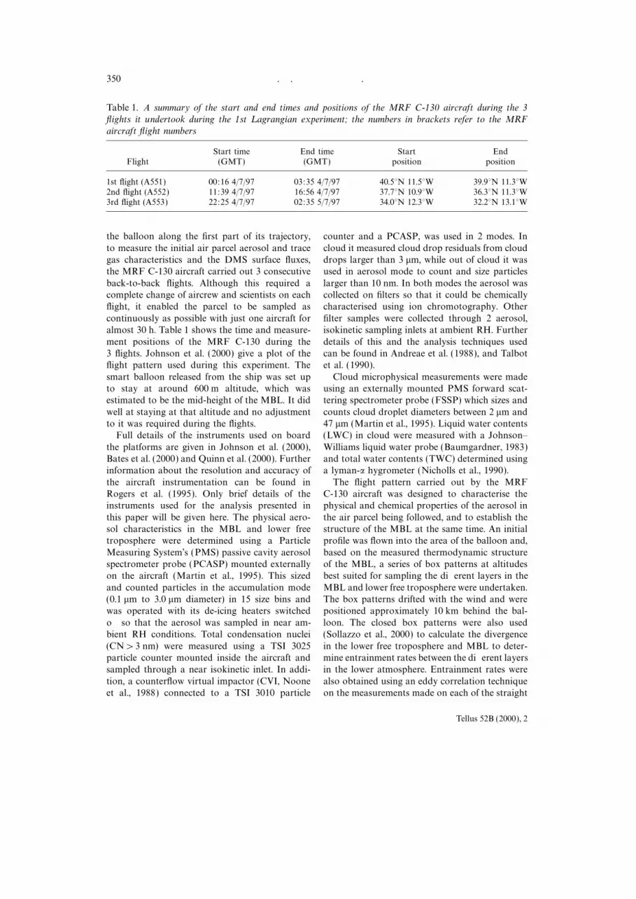
Table 1. A summary of the start and end times and positions of the MRF C-130 aircraft during the 3flights it undertook during the 1st L agrangian experiment; the numbers in brackets refer to the MRFaircraft flight numbers

Start time End time Start EndFlight (GMT) (GMT) position position

1st flight (A551) 00:16 4/7/97 03:35 4/7/97 40.5°N 11.5°W 39.9°N 11.3°W2nd flight (A552) 11:39 4/7/97 16:56 4/7/97 37.7°N 10.9°W 36.3°N 11.3°W3rd flight (A553) 22:25 4/7/97 02:35 5/7/97 34.0°N 12.3°W 32.2°N 13.1°W

the balloon along the first part of its trajectory, counter and a PCASP, was used in 2 modes. In

cloud it measured cloud drop residuals from cloudto measure the initial air parcel aerosol and tracegas characteristics and the DMS surface fluxes, drops larger than 3 mm, while out of cloud it was

used in aerosol mode to count and size particlesthe MRF C-130 aircraft carried out 3 consecutive

back-to-back flights. Although this required a larger than 10 nm. In both modes the aerosol wascollected on filters so that it could be chemicallycomplete change of aircrew and scientists on each

flight, it enabled the parcel to be sampled as characterised using ion chromotography. Other

filter samples were collected through 2 aerosol,continuously as possible with just one aircraft foralmost 30 h. Table 1 shows the time and measure- isokinetic sampling inlets at ambient RH. Further

details of this and the analysis techniques usedment positions of the MRF C-130 during the3 flights. Johnson et al. (2000) give a plot of the can be found in Andreae et al. (1988), and Talbot

et al. (1990).flight pattern used during this experiment. The

smart balloon released from the ship was set up Cloud microphysical measurements were madeusing an externally mounted PMS forward scat-to stay at around 600 m altitude, which was

estimated to be the mid-height of the MBL. It did tering spectrometer probe (FSSP) which sizes and

counts cloud droplet diameters between 2 mm andwell at staying at that altitude and no adjustmentto it was required during the flights. 47 mm (Martin et al., 1995). Liquid water contents

(LWC) in cloud were measured with a Johnson–Full details of the instruments used on board

the platforms are given in Johnson et al. (2000), Williams liquid water probe (Baumgardner, 1983)and total water contents (TWC) determined usingBates et al. (2000) and Quinn et al. (2000). Further

information about the resolution and accuracy of a lyman-a hygrometer (Nicholls et al., 1990).

The flight pattern carried out by the MRFthe aircraft instrumentation can be found inRogers et al. (1995). Only brief details of the C-130 aircraft was designed to characterise the

physical and chemical properties of the aerosol ininstruments used for the analysis presented in

this paper will be given here. The physical aero- the air parcel being followed, and to establish thestructure of the MBL at the same time. An initialsol characteristics in the MBL and lower free

troposphere were determined using a Particle profile was flown into the area of the balloon and,

based on the measured thermodynamic structureMeasuring System’s (PMS) passive cavity aerosolspectrometer probe (PCASP) mounted externally of the MBL, a series of box patterns at altitudes

best suited for sampling the different layers in theon the aircraft (Martin et al., 1995). This sized

and counted particles in the accumulation mode MBL and lower free troposphere were undertaken.The box patterns drifted with the wind and were(0.1 mm to 3.0 mm diameter) in 15 size bins and

was operated with its de-icing heaters switched positioned approximately 10 km behind the bal-

loon. The closed box patterns were also usedoff so that the aerosol was sampled in near am-bient RH conditions. Total condensation nuclei (Sollazzo et al., 2000) to calculate the divergence

in the lower free troposphere and MBL to deter-(CN>3 nm) were measured using a TSI 3025particle counter mounted inside the aircraft and mine entrainment rates between the different layers

in the lower atmosphere. Entrainment rates weresampled through a near isokinetic inlet. In addi-

tion, a counterflow virtual impactor (CVI, Noone also obtained using an eddy correlation techniqueon the measurements made on each of the straightet al., 1988) connected to a TSI 3010 particle

Tellus 52B (2000), 2

351

and level runs of the box patterns. All of themeasurements presented in this paper can befound in the ACE-2 data archive at the Joint

Research Center in Ispra, Italy.

3. Origin of air mass

At mid-day on 4 July 1997, a large anticyclone

was positioned just to the north of the Azores andsignificant ridging to the west of Ireland wasoccurring behind a weakening cold front. Thus

the wind off the coast of Portugal was from thenorthwest but became more north easterly overthe Canary Islands. Verver et al. (2000) show a

more detailed analysis of the synoptic situationduring this experiment. Three-dimensional backtrajectories calculated from NCEP analyses

(Draxler and Hess, 1997 — HYSPLIT4 program), Fig. 1. A METEOSAT visible satellite picture for theand shown in Johnson et al. (2000), indicate that ACE-2 area for mid-day on 4 July 1997 during the 1st

Lagrangian experiment. Superimposed on the picture arethe air originated over the centre of the Northair parcel model back trajectories starting at the top ofAtlantic and did not pass over land in the previousthe boundary layer as the balloon passes under it. The5 days. Thus, the air was relatively clean andstar indicates the position of the balloon at the time of

maritime in origin. The trajectories also indicatethe picture. The dotted trajectory, which passes over the

there was significant subsidence (0.45 cm s−1 on Canary Islands is a model trajectory of the air at theaverage) occurring in the free troposphere. Fig. 1 altitude of the balloon in the SML. A more detailed

explanation and description of these trajectories can beshows a METEOSAT satellite picture of the areafound in Johnson et al. (2000).with the back trajectories superimposed on it.

Most of the trajectories shown end at the top of

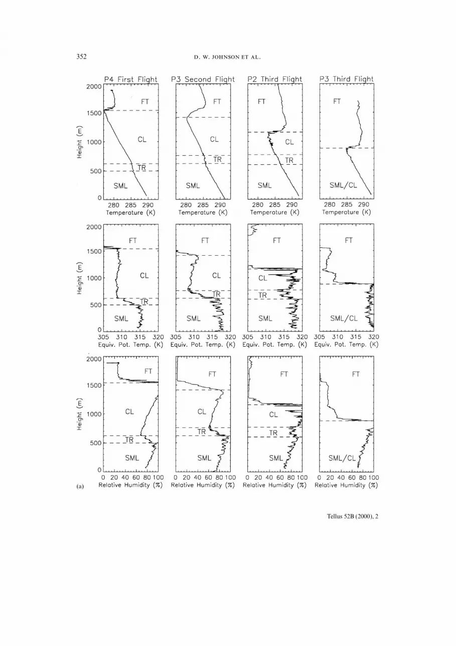
the MBL as the balloon passes underneath it and free troposphere throughout the experiment.Initially, the MBL was relatively deep and multi-the star indicates the position of the balloon at

the time of the satellite picture. The area to the layered, and capped by a 3 K temperature inver-

sion underneath which was a well-broken layer ofnorth effected by the anticyclone was covered witha layer of stratocumulus. However, in the south- stratocumulus. There was a moist, shallow, surface

mixed layer (SML) that extended up to 500 m.eastern part of the anticyclone the cloud was

broken and convective in appearance and off the Above it there was a second mixed layer (CL —cloud layer) which was capped by the cloud andcoast of southwest Portugal the skies were

cloud-free. separated from the SML by a shallow stable

transition region (TR). Well scattered cumulusclouds were observed to grow from the top of theSML, which was conditionally unstable, and some4. Thermodynamic and dynamic evolution

of the MBL extended up to the subsidence inversion wherethey flattened out into the stratocumulus cloudlayer that was mostly likely formed by theDue to the relatively large subsidence rates

occurring in the free troposphere, the height of spreading out of the cumuli. These features canbest be seen in the profile of equivalent potentialthe MBL changed considerably during the experi-

ment. The depth of the MBL decreased from over temperature (he) for the 1st flight shown in Fig. 2.The 2 well-mixed layers are characterised by con-1500 m at the start of the experiment, to less than

900 m at the end. Fig. 2 shows selected profiles stant values of he ; 315 K in the SML and 309 K

in the CL. The broken nature of the cloud canfrom the three MRF C-130 flights which detailsthe change in structure of the MBL and lower also be clearly seen in Fig. 1.

Tellus 52B (2000), 2

. . .352

Tellus 52B (2000), 2

353

Fig. 2 (cont’d).

During the last 2 flights, the height of the TWC in the CL is around 6.5 g/kg, which is muchlower than that found in the SML that starts atinversion progressively decreased and strength-

ened to between 5 K and 6 K. In profile P3 of the approximately 9.1 g/kg and slowly rises with time

to approximately 9.5 g/kg. In the SML, and CL2nd flight (Fig. 2) no cloud was encountered underthe subsidence inversion. Here the inversion is the RH is observed to linearly increase with height

with almost a step change in the TR. The surfacedeeper with a smaller temperature gradient. The

Fig. 2. (a) MRF C-130 aircraft profiles from the 3 flights in the 1st Lagrangian experiment. The first column showsprofile P4 (0254 GMT 4 July 1997) from the 1st flight, the second column profile P3 (1453 GMT 4 July 1997) fromthe 2nd flight, and the third and fourth columns profile P2 (2225 GMT on 4 July 1997) and P3 (02:13 GMT 5 July1997) respectively from the 3rd flight. The first row shows temperature, the second equivalent potential temperature,the third relative humidity. The horizontal dashed lines indicate the top and bottom of the layers observed in theboundary layer, i.e., the surface mixed layer (SML), the cloud layer (CL), the transition region between the SMLand the CL (TR), and the free troposphere (FT). (b) Same as (a) except the first row shows liquid water contentand the second row ozone concentration.

Tellus 52B (2000), 2

. . .354

RH is generally around 70% but at the time of generated increased turbulent kinetic energy andenhanced mixing in the SML.the balloon release, the ship reported the RH to

be 83%. (b) An increase in the sea surface temperature

(SST) along the length of the balloons trajectoryIn contrast to the MBL, the SML deepensduring the 3 flights. At the beginning of the which increased surface heat fluxes.experiment, the SML has a depth of 500 m but as

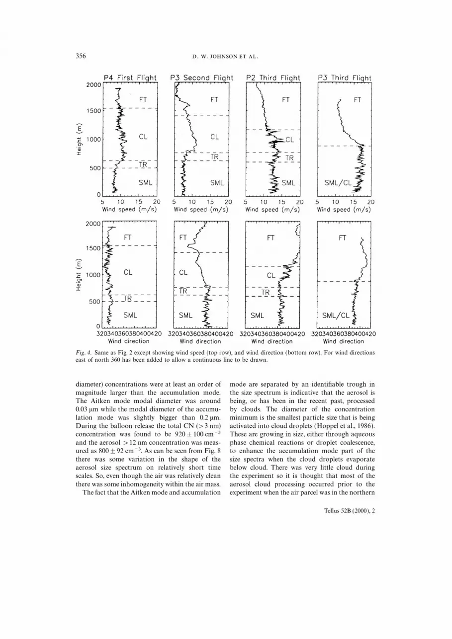
Fig. 4 shows aircraft profiles of wind speed andthe experiment progresses it gets deeper until direction during the experiment. Again, the layeredduring the 3rd flight it is observed to merge with

structure of the MBL can be identified. In thethe subsidence inversion at 900 m. This accords

SML, the wind speed and direction is constant inwith the measurements of cloud penetrations and the vertical but it increases significantly with time,observations from the flight deck, which showed

from 8 m s−1 to 16 m s−1, and the direction veersthat on the 1st flight, the cumulus clouds encoun-

from 330° to 030°. These are all in agreement withtered had a large vertical extent and some of them the trajectory of the balloon, which was in thewere flattening out into stratocumulus underneath

SML, except near the start of the 1st flight wherethe inversion. On the 2nd flight, during the middle

it was probably in the TR between the SML andof the day on 4 July, the cumulus clouds were the CL (see Johnson and Businger, 2000).small and well scattered, though on the 3rd flight,

Generally, the wind speed was higher in the CLon the night of the 4/5 July, more clouds were

compared to the SML and there was often verticalencountered but their vertical extent was limited wind shear through the TR, the CL and theand the cumuli were more prone to flattening out

subsidence inversion.into stratocumulus, until in the very final profile The SST was determined using the aircraftof the experiment only shallow, broken stratocu- Heimann KT remote radiometer at the lowestmulus was seen. This is borne out in Fig. 2 that

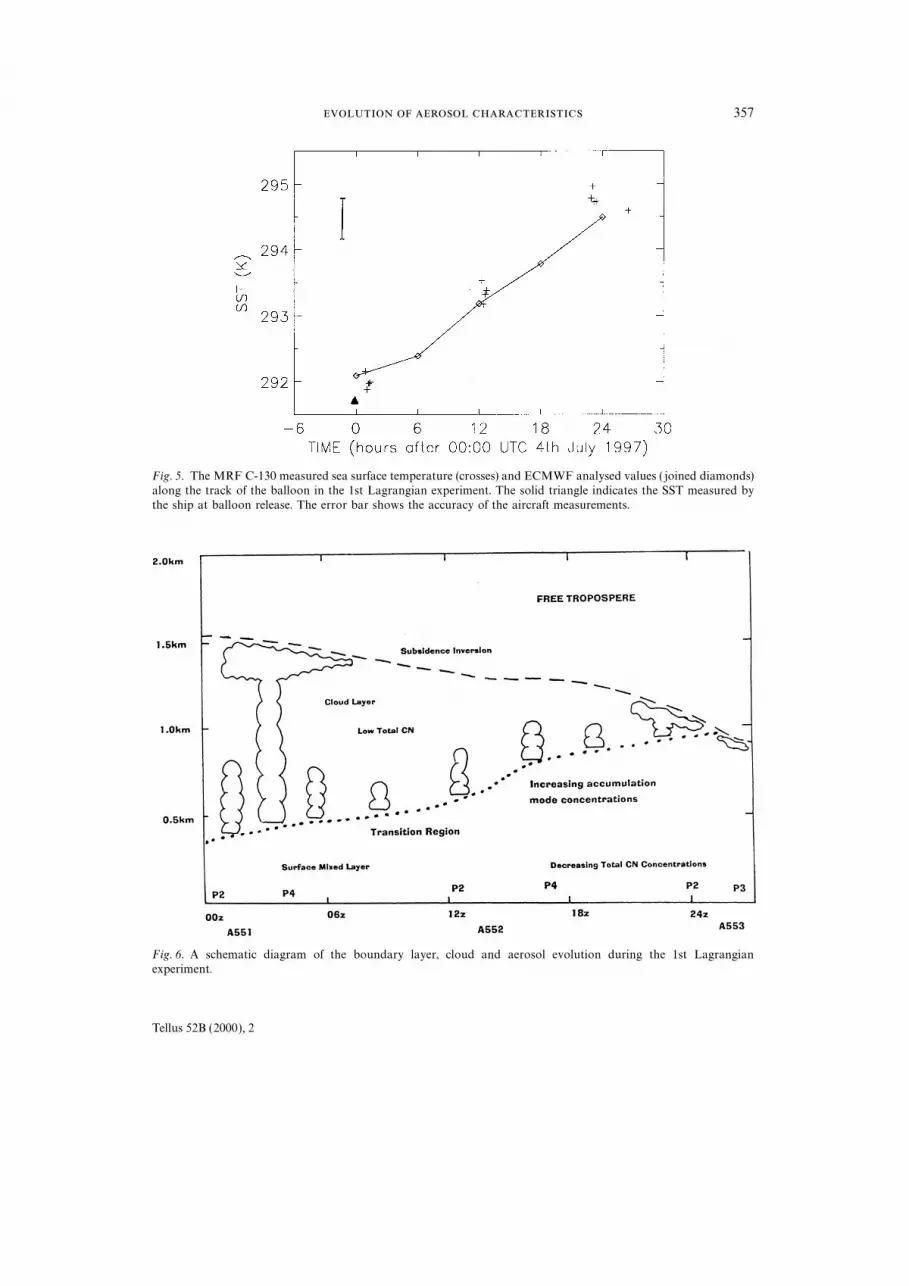
point in each of its profiles and in the lowest boxshows LWC profiles. In half the profiles (not all patterns. The variation of SST is shown in Fig. 5,are shown in Fig. 2), the aircraft did not pass with the ECMWF analysed SST which agree tothrough any cloud. The LWC profile during P4

within 0.5 K. It can be seen that the SST increasesof the 1st flight and P3 of the 3rd flight is from 292 K to almost 295 K. This in combinationcharacteristic of a stratocumulus sheet, whereas with the surface water vapour flux helps to raisethe other cloud penetrations look more like you

the SML he from 315 K to 319 K.would expect to see when passing through cumuli A schematic diagram summarising the evolutionunderlying stratocumulus as can be seen in profile

of the MBL structure and cloud characteristicsP2 of the 3rd flight.

throughout the 1st Lagrangian experiment isTo show how the structure of the MBL evolved shown in Fig. 6. This is based on evidence from

in a more continuous fashion, the measurementsall the profiles and box patterns carried out by

made in all the aircraft profiles, have been inter-the aircraft, and on the manually recorded obser-

polated onto a grid so that vertical-time cross- vations made by the aircraft scientists duringsections can be constructed. This is shown in

the flights.Fig. 3 for he . The analysis has necessitated some

data smoothing so that the fine detail has beenlost but the overall large scale changes remain. 5. Evolution of aerosol in the MBLThe sharp change in height of the base of the

subsidence inversion from 1500 m to 900 m during Not surprisingly, considering the changes in thethermodynamic and dynamic structure of thethe experiment can be seen, and as the subsidence

continues in the free troposphere the inversion at MBL during the experiment, some dramatic

changes were observed in the aerosol character-the top of the MBL strengthens. It also showswell the stable region between the SML and the istics. The most startling change was a quadru-

pling of the number concentration of accumulationwell-mixed CL and the SML depth increasingwith time. The increase in depth of the SML is mode (0.1 mm to 3.0 mm diameter) aerosol particles

in the MBL. Fig. 7 shows profiles of the accumula-probably due to a combination of 2 things:

tion mode concentration (N) and mean volumediameter. In the 1st flight, the SML was clean(a) An increase in the surface wind speed that

Tellus 52B (2000), 2

355

Fig. 3. The variation of equivalent potential temperature (K) in the lower atmosphere during the 1st Lagrangianexperiment measured by the MRF C-130.

with accumulation mode concentrations of MBL but also has the potential to increase saltparticle production at the sea surface due to50 cm−3 and there was very little change between

the MBL and lower free troposphere. By the end breaking waves. It is commonly agreed that oncethe wind speed exceeds 8 m s−1 salt particle pro-of the 3rd flight though, this had increased to

200 cm−3. In contrast, variations in the lower free duction increases sharply (Woodcock, 1953;

O’Dowd and Smith, 1993). During the 2nd flighttroposphere were only small. Thus, by the end ofthe experiment there was a relatively sharp gradi- (during daylight hours), ‘‘white capping’’ at the

surface was widely observed. A time scale analysisent in accumulation mode aerosol concentrations

across the inversion. The double layer structure carried out by Hoell et al. (2000) estimate thatthe changing wind conditions during the 26-hof the MBL had little effect on the accumulation

mode concentrations that seemed to be well mixed period of the experiment could contribute an extra

accumulation mode concentration of 108 cm−3,throughout the depth of the MBL. However, themean volume radius of the accumulation mode which is the same order of magnitude as the

observed 150 cm−3 concentration increase. Table 2particles did vary in the vertical. The largest

particles are found in the SML and the smallest summarises the mean aerosol and wind character-istics measured during the aircraft box patterns inin the free troposphere. Intermediate size particles

are found in the cloud layer. the various layers of the lower atmosphere.Fig. 8 shows the dry, aerosol size spectrum atA large majority of the increase in accumulation

mode aerosol concentrations can be explained by the surface measured by the ship, on either side

of the balloon release. This has a marked bimodalthe increase in surface wind speed. This not onlyhelped to enhance mechanical mixing within the shape and the Aitken mode (0.01 mm to 0.1 mm

Tellus 52B (2000), 2

. . .356

Fig. 4. Same as Fig. 2 except showing wind speed (top row), and wind direction (bottom row). For wind directionseast of north 360 has been added to allow a continuous line to be drawn.

diameter) concentrations were at least an order of mode are separated by an identifiable trough in

the size spectrum is indicative that the aerosol ismagnitude larger than the accumulation mode.The Aitken mode modal diameter was around being, or has been in the recent past, processed

by clouds. The diameter of the concentration0.03 mm while the modal diameter of the accumu-

lation mode was slightly bigger than 0.2 mm. minimum is the smallest particle size that is beingactivated into cloud droplets (Hoppel et al., 1986).During the balloon release the total CN (>3 nm)

concentration was found to be 920±100 cm−3 These are growing in size, either through aqueous

phase chemical reactions or droplet coalescence,and the aerosol >12 nm concentration was meas-ured as 800±92 cm−3. As can be seen from Fig. 8 to enhance the accumulation mode part of the

size spectra when the cloud droplets evaporatethere was some variation in the shape of theaerosol size spectrum on relatively short time below cloud. There was very little cloud during

the experiment so it is thought that most of thescales. So, even though the air was relatively clean

there was some inhomogeneity within the air mass. aerosol cloud processing occurred prior to theexperiment when the air parcel was in the northernThe fact that the Aitken mode and accumulation

Tellus 52B (2000), 2

357

Fig. 5. The MRF C-130 measured sea surface temperature (crosses) and ECMWF analysed values ( joined diamonds)along the track of the balloon in the 1st Lagrangian experiment. The solid triangle indicates the SST measured bythe ship at balloon release. The error bar shows the accuracy of the aircraft measurements.

Fig. 6. A schematic diagram of the boundary layer, cloud and aerosol evolution during the 1st Lagrangianexperiment.

Tellus 52B (2000), 2

. . .358

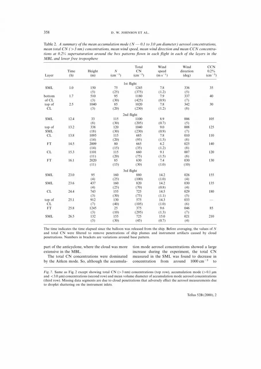
Table 2. A summary of the mean accumulation mode (N — 0.1 to 3.0 mm diameter) aerosol concentrations,mean total CN (>3 nm) concentrations, mean wind speed, mean wind direction and mean CCN concentra-tions at 0.2% supersaturation around the box patterns flown in each flight in each of the layers in theMBL and lower free troposphere

Total Wind Wind CCNTime Height N CN speed direction 0.2%

Layer (h) (m) (cm−3 ) (cm−3 ) (m s−1 ) (deg) (cm−3 )1st flight

SML 1.0 150 75 1245 7.8 336 35(5) (25) (375) (1.2) (5)

bottom 1.7 510 95 1180 7.9 337 40of CL (3) (30) (425) (0.9) (7)top of 2.5 1040 85 1020 7.8 342 30CL (3) (20) (230) (1.2) (8)

2nd flightSML 12.4 33 115 1100 8.9 006 105

(8) (30) (205) (0.7) (5)top of 13.2 338 120 1040 9.0 008 125SML (18) (30) (230) (0.9) (7)CL 13.8 1095 115 685 7.8 010 110

(14) (20) (95) (1.5) (8)FT 14.5 2009 80 665 6.2 025 140

(14) (15) (35) (1.2) (8)CL 15.3 1101 115 660 9.1 007 120

(11) (20) (75) (1.5) (8)FT 16.1 2020 85 630 7.4 030 130

(11) (15) (30) (1.0) (10)

3rd flightSML 23.0 95 160 880 14.2 026 155

(4) (25) (100) (1.0) (4)SML 23.6 437 160 820 14.2 030 135

(4) (25) (70) (0.8) (4)CL 24.4 743 155 725 14.5 029 180

(3) (30) (75) (1.1) (5)top of 25.1 912 130 575 14.3 033 —CL (7) (40) (105) (1.0) (6)FT 25.8 1245 25 375 9.6 046 85

(3) (10) (295) (1.3) (7)SML 26.5 132 155 725 15.0 021 210

(5) (30) (45) (0.7) (4)

The time indicates the time elapsed since the balloon was released from the ship. Before averaging, the values of Nand total CN were filtered to remove penetrations of ship plumes and instrument artifacts caused by cloudpenetrations. Numbers in brackets are variations around base pattern.

part of the anticyclone, where the cloud was more tion mode aerosol concentrations showed a largeincrease during the experiment, the total CNextensive in the MBL.

The total CN concentrations were dominated measured in the SML was found to decrease in

concentration from around 1000 cm−3 toby the Aitken mode. So, although the accumula-

Fig. 7. Same as Fig. 2 except showing total CN (>3 nm) concentrations (top row), accumulation mode (>0.1 mmand <3.0 mm) concentrations (second row) and mean volume diameter of accumulation mode aerosol concentrations(third row). Missing data segments are due to cloud penetrations that adversely effect the aerosol measurements dueto droplet shattering on the instrument inlets.

Tellus 52B (2000), 2

359

Tellus 52B (2000), 2

. . .360

Fig. 8. The variation of the aerosol size spectra measured by the R/V Vodyanitskiy an hour either side of the releaseof the constant height ‘‘smart’’ balloons at the start of the 1st Lagrangian experiment. The aerosol was dried to aRH of 50%. All times are in GMT.

750 cm−3. This can be seen in the aircraft profiles to understand where a pollution layer would havecome from. New particle nucleation in the uppershown in Fig. 7. Also, in contrast to the accumula-

tion mode aerosol, the multiple layering of the free troposphere (Raes, 1995) which had subsidedis similarly unlikely, as the high aerosol concentra-MBL had a pronounced effect on the total CN

concentrations. The CL showed much greater tion layer is associated with a relatively high heand RH. The layer may be similar to that observedvariations in total CN concentrations and there

were several hundred fewer particles in the CL by Hegg et al. (1990) and Clarke et al. (1998)during ACE-1 where it was found that nucleationcompared to the SML. However, as the SML got

deeper during the course of the experiment the was occurring in the outflow regions from cumuli,although the measurements presented here werevertical profiles of total CN concentration show

far less variation. made during the night. It is possible that some of

the cumuli in the MBL had overshot the top ofThe total CN concentrations in the lower freetroposphere are around 500 cm−3 but there is the MBL and detrained into the inversion layer.

This would help explain the higher RH and hesome variation during the flights. In the 3rd flight,

there is a marked change in the characteristics of values that were in effect diluted MBL air.The majority of the increase in the accumulationthe total CN above the MBL in profile P3. Just

above the subsidence inversion base and the top mode concentrations occurs in the size range

0.1 mm to 0.3 mm diameter. This can be seen inof the stratocumulus, a layer of high aerosolconcentrations is found over a depth of 200 m. the size spectra shown in Fig. 9. Here a comparison

of the evolution of the aerosol size spectra in theThe peak concentrations are around 2670 cm−3(off the edge of Fig. 7). We are confident this was SML, CL and lower free troposphere is shown.

Each size spectrum plotted is the average alongnot an instrument artifact as the layer was flown

through on a couple of occasions and its character- one run of a box pattern in the indicated layer.This is also borne out in Fig. 10 which showsistics were similar each time. Differential hori-

zontal advection of aerosol maybe the cause, but measurements of the accumulation mode spectra

from the CVI in aerosol mode underneath cloudas the MBL air parcel was considered to beembedded in a large maritime air mass it is difficult in the SML for each of the 3 flights. In the last

Tellus 52B (2000), 2

361

Fig. 9. The variation of accumulation mode (>0.1 mm and <3.0 mm) and coarse mode (>3.0 mm) aerosol size spectrameasured with the MRF C-130 PCASP and FSSP respectively during the 3 flights in the 1st Lagrangian experimentin the surface mixed layer, cloud layer and lower free troposphere. The top row shows aerosol concentration andthe bottom row, aerosol surface area. The aerosol was sampled at ambient RH.

Fig. 10. The variation of accumulation mode (>0.1 mm and <3.0 mm) aerosol size spectra measured with the MRFC-130 CVI in aerosol mode during the 3 flights in the 1st Lagrangian experiment in the surface mixed layer.

Tellus 52B (2000), 2

. . .362

flight there is evidence of a small increase in the Fig. 12 shows time series of accumulation modeaerosol concentrations, wind speed, total CN con-larger particles (>0.4 mm diameter). The mode

diameter in each of the spectra decreases as the centrations and RH around boxes flown in the

SML. The RH is relatively homogeneous in eachconcentrations get higher. O’Dowd and Smith(1993) found that in clean air masses, submicron of the flights, being about 70% in the 2nd and the

3rd flights and 80% in the first one. The largesea salt aerosol concentrations showed a strong

exponential increase with high wind speeds down changes in accumulation mode aerosol concentra-tions between flights appear well correlated withto a dry particle diameter of 0.1 mm, which is very

similar to what is being observed here. For the the major changes in wind speed. In fact, the local

variation of wind speed and accumulation modefirst time in these experiments it has been possibleto follow the evolution of the aerosol character- aerosol concentration is also of some interest here.

During the box patterns in the SML in the 2ndistics under changing wind conditions, whereas in

previous experiments only spot measurements of and 3rd flights, the wind speeds were high enoughfor significant white capping of the waves to beaerosol concentrations on different days under

different wind conditions have been reported. occurring. In the 1st flight, however the wind

speed varied between 5 m s−1 and almost 10 m s−1There is a clear correlation here between increas-ing wind speed and increasing submicron aerosol indicating perhaps that during the course of this

box a significant increase in salt particle produc-concentrations. This can be seen in Fig. 11.

Fig. 11. A plot of wind speed against accumulation mode concentrations averaged over 20 s in box patterns flownnear the bottom of the SML in each of the flights. Dots represent the 1st flight, crosses the 2nd flight and trianglesthe 3rd flight in the 1st Lagrangian experiment.

Tellus 52B (2000), 2

363

Fig. 12. Time series of accumulation mode (>0.1 mm and <3.0 mm) aerosol concentration (top diagram), wind speed(second diagram), total CN (>3 nm) concentrations (third diagram), and relative humidity (bottom diagram) aroundone of the MRF C-130 box patterns in the surface mixed layer during the 1st flight (dashed line), 2nd flight (dottedline), and 3rd flight (solid line) in the 1st Lagrangian experiment. The x-axis indicates the time from the start of thebox pattern in seconds.

Tellus 52B (2000), 2

. . .364

Fig. 13. A scatter plot of accumulation mode (>0.1 mm and <3.0 mm) aerosol concentration and total CN (>3 nm)concentration measured around one of the MRF C-130 box patterns in the surface mixed layer of the 1st flight inthe 1st Lagrangian experiment.

tion would be initiated. There is certainly an aerosol surface area produced by the source of

salt particles is enhancing the coagulation of accu-increase in accumulation mode aerosol concentra-tions from less than 50 cm−3 to over 100 cm−3 mulation mode and Aitken mode particles.

Therefore as the accumulation mode aerosol par-during this run, which is in phase with the change

in wind speed. The increase in salt particle surface ticles increase in concentration due to the increas-ing wind speed, they are sweeping out more Aitkenarea that this produces (see Fig. 9) has the poten-

tial to disrupt or modify the processes which were mode particles and as a result the total CN

concentrations are decreasing. The anti-correla-in pseudo equilibrium before the wind speedstarted to increase. This may help to explain why tion of these 2 parameters is not as noticeable at

other times in the flight. This should not bethe total CN concentrations during this box are

anti-correlated to the wind speed and accumula- unexpected. The onset of significant salt particleproduction will have a major disruptive effect ontion mode aerosol concentrations. The total CN

concentrations decrease from over 1700 cm−3 to the balance of the different aerosol processes

occurring in the MBL. Once a continuous supply600 cm−3 in this time.Fig. 13 shows a scatter plot of accumulation of salt particles has begun then a new process

balance will be achieved.mode aerosol concentrations and total CN con-

centrations in the box pattern in the SML in the It should be noted here that during the box inthe 1st flight (800 s from the start of the box) the1st flight. The anti-correlation between these para-

meters is very marked. It is difficult from the aircraft flew through a plume from a ship in thebusy shipping lanes off the coast of Portugal. Atobservations alone to determine what processes

are occurring here. Further analysis and compar- this stage, the plume was very narrow (i.e., the

penetration of the plume was close to the ship)ison with simulations from process models isrequired but we hypothesize that the increased and the peak concentration was several thousand

Tellus 52B (2000), 2

365

particles cm−3. During the 2nd flight a broader Typically in this sort of MBL the maximumplume, at a similar number of seconds from the start water supersaturation that would be achieved nearof the box was penetrated. Here the peak concentra- cloud base would be ~0.3% (Martin et al., 1994).tion was only 70 cm−3 above background levels due From these spectra, this supersaturation wouldto the plume being diluted with distance down- produce droplet concentrations of approximatelystream from the ship. A weaker plume still was also 50 cm−3 in the 1st flight whereas in the last 2observed on the 3rd flight about 1100 s from the flights it would produce droplet concentrationsstart of the box. These observations give us a great above 150 cm−3. This change in the CCN charac-deal of confidence that the aircraft was following teristics is evidenced in the change in the cloudthe same parcel of air on each flight. microphysics. Fig. 15 show profiles of droplet con-

centrations, measured by an FSSP, and accumula-

tion mode aerosol concentrations measured in the6. Evolution of the cloud microphysicsfirst and last flight of the experiment. In addition,in the MBLFig. 16 shows droplet spectra averaged over 30 m

of cloud at the top of the MBL for the sameThe increase in the accumulation mode concen-profiles. When the air in the MBL is very cleantrations observed in this experiment has a markedat the start of the experiment, the clouds hadeffect on the cloud condensation nuclei (CCN)droplet concentrations of 60 cm−3 whereas at theconcentrations in the MBL. Fig. 14 shows CCNend of the experiment the cloud droplet concentra-supersaturation spectra measured with a thermaltions had doubled to 120 cm−3. Measurementsgradient diffusion chamber in the SML in eachfrom the CVI of the droplet residual particleflight. The 2nd and 3rd flights have significantlyspectra also indicate that droplet concentrationshigher CCN concentrations than the first one.in the stratocumulus in the 3rd flight were moreLarger supersaturations tend to activate smallerthan 120 cm−3. These droplet concentrations com-aerosol particles. Therefore, the change in gradientbined with the measured supersaturation spectrathat is observed in the supersaturation spectraindicate that the maximum supersaturation in thewith time indicates that higher concentrations ofcloud in the 1st flight was around 0.4% while insmall accumulation mode particles were being

produced. the last flight it was 0.18%. This indicates that

Fig. 14. CCN supersaturation spectra measured in the surface mixed layer in each of the 3 flights of the MRF C-130in the 1st Lagrangian experiment.

Tellus 52B (2000), 2

. . .366

Fig. 15. Same as Fig. 2 except showing accumulation mode (>0.1 mm and <3.0 mm) aerosol concentrations (N,dotted line) and cloud droplet concentrations (ND, solid line) (top row), and cloud droplet effective radius(bottom row).

there was either much weaker overturning occur- ticles are not big enough to be activated at thereduced maximum supersaturations or entrain-ring in the later part of the experiment or the

maximum supersaturation was being suppressed ment of dry, clean free tropospheric air into the

cloud top is suppressing the cloud droplet concen-by the increased activation of larger numbers ofaerosol particles into water droplets. trations. There is evidence that both of these

processes are occurring. This change in the aerosolIn the 1st flight all of the accumulation mode

aerosol particles are being activated as can be and cloud microphysics has a marked effect onthe shape of the cloud droplet size spectrum. Inseen by the 151 ratio of these parameters in

Fig. 15. However, in the 3rd flight although the the 1st flight, the size spectrum has a classicalclean air mass shape with a prominent mode atcloud droplet concentration increases it does not

match the quadrupling of the accumulation mode around 18 mm. In the final flight the modal dia-

meter is decreased to less than 10 mm and isconcentration. This could be for one of 2 reasons.Either some of the new sub-micron sea salt par- beginning to take on more of the appearance of a

Tellus 52B (2000), 2

367

Fig. 16. A comparison of cloud droplet size spectra during MRF C-130 cloud penetrations near the top of theboundary layer in each of the 3 flights in the 1st Lagrangian experiment.

slightly dirty cloud with more of a uni-modal the molar mixing ratios of the soluble fine mode

appearance. This change in shape of the spectra aerosol. The ratio of ammonium to sulphatereduces the maximum effective radius (Re — the mixing ratio measurements is generally a littleratio of the third moment of the spectra to the greater than 2 indicative of ammonium sulphatesecond moment (Martin et al., 1994)) measured at being present in the parcel of air. There is a smallcloud top during the experiment; as seen in Fig. 15. tendency for the ammonium sulphate to increaseRe in the 1st flight has a maximum value of 10 mm during the course of the experiment. The nextwhereas in the last flight it is reduced to 8 mm. As largest component of the soluble fine mode aerosolthere is little change in the liquid water path of is sea salt and this is found to increase significantlythese clouds the changes in droplet size and as would be expected due to the observed increasenumber concentration will have a significant effect in wind speed.on the radiative characteristics of the cloud. The Sea salt dominates the soluble coarse modeclouds will have a progressively higher albedo (>1.4 mm diameter) aerosol. Table 4 presents theduring the experiment. molar mixing ratios of the soluble coarse mode

aerosol. While the absolute concentrations of the

sea salt species in the coarse mode are only about7. The chemical characteristics of the aerosol one third of the actual values because of inlet

and trace gases losses, the relative amounts between samples are

valid indicators of the change in sea salt fractional7.1. Aerosol chemistry

mass. In both the fine mode and coarse mode

aerosol results there seems to be very little consist-The ion chromatography analysis of the filtersent variation of either ammonium sulphate or seacollected on the aircraft show that the soluble fineparticle concentrations with height in the MBL.mode (<1.4 mm diameter) aerosol has a large

component of ammonium sulphate. Table 3 shows The mixing between the SML and the CL appears

Tellus 52B (2000), 2

. . .368

Table 3. Concentrations (ppt molar mixing ratios) of soluble fine mode (<1.4 mm diameter) aerosol com-position measured during the 1st L agrangian experiment using filters exposed on the MRF C-130 aircraftin specific layers of the boundary layer (SML — surface mixed layer, and CL — cloud layer) and freetroposphere (FT). T he numbers in brackets refer to the uncertainty in the analysis

Layer Na+ NH+4 K+ Mg++ Ca++ MSA Cl− NO−3 SO2−41st flight

SML 61 187 <40 <20 <60 <5 76 34 60(63) (16) (40) (18) (52) (4) (46) (31) (18)

CL 702 153 <40 28 <50 <3 656 36 72(55) (13) (35) (16) (46) (3) (50) (27) (16)

FT <30 115 <20 <10 <25 <3 <20 12 39(28) (9) (18) (8) (23) (2) (20) (14) (8)

SML 95 211 21 <10 <70 <3 159 18 104(39) (16) (14) (12) (67) (3) (29) (14) (7)

2nd flighttop of 64 316 <30 21 25 <5 162 46 127SML (66) (24) (24) (20) (113) (5) (48) (24) (10)CL 267 242 99 84 355 <5 213 50 125

(58) (19) (21) (18) (99) (4) (42) (21) (9)FT <70 145 <30 <20 <120 <5 <50 46 51

(63) (13) (23) (19) (107) (5) (46) (23) (10)

3rd flightSML 101 259 <50 29 105 <5 194 33 111

(82) (19) (46) (17) (41) (4) (29) (32) (15)top of 196 207 <40 25 <30 <3 265 48 106SML (64) (15) (36) (13) (32) (3) (24) (25) (12)CL 191 212 <40 31 <30 <3 272 19 104

(67) (16) (37) (14) (33) (3) (25) (26) (12)top of 200 113 <30 22 <30 <3 227 <20 62CL (45) (9) (25) (9) (23) (2) (20) (18) (8)FT <90 67 <50 <20 57 <5 30 <40 29

(87) (8) (48) (18) (44) (4) (31) (34) (16)

to be occurring on shorter time scales than the However, both sets of filters also suggest that the

non-sea salt sulphate increases between 10% (CVIlifetime of the aerosol particles and so a well-mixed MBL in terms of the aerosol composition filters) and 50% (filter packs) during the course of

the experiment. This indicates that sulphate massis being maintained. It is speculated that the

cumulus clouds are playing a role here. These will must be being produced locally. The small concen-trations of SO2 available in the MBL are enoughlocally rapidly mix SML air which is dragged up

into the CL, and then the broader downdraughts for either aqueous phase chemistry in the cloud

droplets to produce sulphate on existing CCN,associated with the cumulus clouds will enhancethe entrainment of CL air back into the SML. thereby improving their CCN characteristics or

by the direct deposition of SO2 onto the aerosolFilter samples collected from the CVI probe in

aerosol mode have also been analysed using an particles below cloud base. The first of theseprocesses would tend to enhance the bimodalion chromatograph technique. Table 5 shows the

mass (mg m−3 ) of aerosol for individual soluble characteristics of the aerosol spectrum by increas-ing mass in the accumulation mode, whereas thespecies. This shows that the sea salt sulphate mass

increases by 50% from the 1st flight to the 3rd latter would tend to fill in the trough between the

Aitken mode and the accumulation mode. Asflight in the SML, consistent with the physicalaerosol measurements made by the aircraft. there is very little observational evidence that the

Tellus 52B (2000), 2

369

Table 4. Concentrations (ppt molar mixing ratios) of soluble large (>1.4 mm diameter) aerosol composi-tion measured during the 1st L agrangian experiment using filters exposed on the MRF C-130 aircraft inspecific layers of the boundary layer (SML — surface mixed layer, and CL — cloud layer) and freetroposphere (FT). T he numbers in brackets refer to the uncertainty in the analysis

Layer Na+ NH+4 K+ Mg++ Ca++ MSA Cl− NO−3 SO2−41st flight

SML 442 <10 <10 46 <20 2.0 347 23 30(7) (7) (7) (7) (21) (3) (25) (7) (2)

CL 201 <10 <10 22 178 <3 159 24 9(8) (8) (8) (8) (23) (3) (27) (8) (2)

FT 389 <10 <10 49 35 2.3 268 69 47(6) (6) (6) (6) (18) (2) (22) (6) (3)

2nd flightSML 530 <5 9 65 22 4.5 364 47 37

(21) (5) (12) (5) (7) (2) (23) (3) (2)top of 712 <10 20 66 37 3.2 552 74 48SML (35) (9) (20) (9) (11) (4) (36) (5) (4)CL 1418 <10 <20 96 15 <3 651 74 51

(31) (8) (18) (8) (10) (3) (41) (5) (3)FT 47 <10 <20 <10 <10 <4 49 <5 <3

(33) (9) (19) (9) (10) (3) (10) (5) (3)

3rd flightSML 806 <10 22 85 35 <3 668 <7 53

(22) (7) (6) (5) (10) (3) (43) (7) (7)top of 410 <5 11 44 7 2.4 335 <5 25SML (17) (5) (4) (3) (8) (2) (22) (5) (5)CL 871 10 33 91 33 <3 690 7 61

(18) (6) (5) (6) (8) (2) (44) (6) (6)top of 358 <5 12 43 22 1.8 259 <4 24CL (12) (4) (3) (3) (5) (2) (17) (4) (4)FT <30 <10 <10 5 <10 <3 <15 <8 <7

(24) (7) (6) (3) (10) (3) (15) (7) (7)

Table 5. Mass (mg m−3) of aerosol for individual soluble species determined from the filters sampling aircollected by the CVI inlet set up in aerosol mode, compared with the mass calculated from the PCASPconnected to the CVI probe using a density of 2 g cm−3OPC Total ionic Sea salt Non-sea saltmass species Na Cl SO4 SO4 NO3 NH4

1st flight10.6 10.5 2.3 4.2 0.62 0.60 0.26 0.13

(±1.9) (±0.3) (±0.2) (±0.1) (±0.03) (±0.02) (±0.01) (±0.02)

3rd flight15 14.4 3.5 6.5 0.93 0.67 1.74 0.37

(±2) (±0.3) (±0.2) (±0.2) (±0.03) (±0.02) (±0.07) (±0.04)

Tellus 52B (2000), 2

. . .370

trough is being filled in, it is likely that much of time, which suggests that the ozone was in adynamic equilibrium. The lower concentrations inthe extra non-sea salt sulphate mass is coming

from cloud processing. The time scale analysis the SML are likely to be a result of dry deposition

to the sea surface and the chemical destructioncarried out by Hoell et al. (2000) also reinforcesthis view as they estimate that under the conditions of ozone in the high RH (McFadyen et al.,

2000). Entrainment of ozone from the CL andof this experiment aqueous phase chemistry will

produce sulphate mass an order of magnitude lower free troposphere will then act as a source ofozone to continually top up the concentrations infaster than simple condensation will.the SML.

H2O2 concentration measurements on the air-craft showed that it rose almost linearly in the

7.2. T race gas chemistrySML from 0.9 ppb to 1.3 ppb. This is not surpris-

ing as the sea surface is a strong sink of H2O2 .SO2 concentrations were determined by theaircraft using filter samples exposed in each of the Through the TR and CL, H2O2 is almost constant

and acts as a source of H2O2 for the SML throughlayers in the MBL and the lower free troposphere.

In general the SO2 levels were low and close to slow entrainment mechanisms. The organic perox-ide concentration decreases throughout the MBLthe detection limit of the technique used and the

concentrations measured on the ship were all from 0.5 ppb at the surface to 0.1 ppb at the top

of the MBL.below the 100 ppt detection limit of their instru-ment. In the SML the concentrations varied During the 1st Lagrangian experiment, 9 bottle

samples from the different layers in the MBL andbetween 17 (±8) and 40 (±18) ppt and in the CLbetween <10 (±4) and 24 (±7) ppt suggesting lower free troposphere were collected for analysis

of NMHCs. Over 90 species of NMHC we estim-that perhaps there is some loss of SO2 through

cloud processing. However, this difference may ated from the samples. However, as would beexpected in a clean air mass the NMHC mixingnot be significant in view of the large analytical

uncertainties associated with the low SO2 values ratios are relatively small and close to back-

ground levels.observed, which were comparable to resultsobtained from remote, unpolluted locations, andwere probably sustained by the oxidation of DMS.

Radon and carbon monoxide were both meas- 8. Summary and conclusionsured by the R/V Vodyanitskiy and the MRF C-130aircraft, respectively. Both were observed to be at The 1st ACE-2 Lagrangian experiment fol-

lowed the evolution of the MBL structure,very low levels, close to or below the detectionlimits of the instruments as would be expected in aerosol and cloud microphysical characteristics

in a clean maritime air mass over a period ofa clean maritime air mass. Ozone and H2O2 are

both important oxidants for the production of 30 h. Significant changes occurred to the parcelof air being followed. Although the MBL startedsulphate through aqueous phase reactions

depending on the water acidity. Both gases were very clean, the accumulation mode aerosol con-

centrations quadrupled during the period of themeasured, although, due to instrument problems,H2O2 was only sampled on the 2nd flight. Included experiment so that the MBL ended up with

relatively high concentrations of CCN for ain Fig. 2 were profiles of ozone concentration from

each of the flights. These showed a significant maritime air mass, while the total CN concentra-tions decreased by 25%. The challenge has been,amount of vertical variability that mirrored the

layered structure of the MBL. The lowest values and will be, to try to explain this. Aerosol

modeling studies of this case are only justwere observed in the SML at around 30 (±4) ppb.This compared well with the ship measurement of beginning, so the main aim of this paper has

been to collate all the measurements made and27 ppb. In the CL, they rose to approximately 40(±4) ppb with an increase across the TR. In the to put forward the best description of the

evolution of the air mass as we can. From this,lower free troposphere, the concentrations were

generally more than 50 (±5) ppb. Very little hypotheses are suggested for the importantprocesses causing the air mass evolution, whichchange in the concentration was observed with

Tellus 52B (2000), 2

371

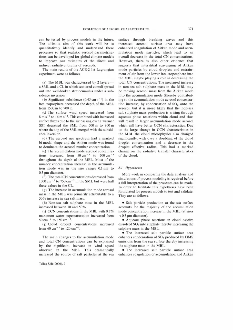
can be tested by process models in the future. surface through breaking waves and thisincreased aerosol surface area may haveThe ultimate aim of this work will be to

quantitatively identify and understand these enhanced coagulation of Aitken mode and accu-

mulation mode particles, which lead to anprocesses so that realistic aerosol parametrisa-tions can be developed for global climate models overall decrease in the total CN concentrations.

However, there is also other evidence thatto improve our estimates of the direct and

indirect radiative forcing of aerosols. suggests that interstitial scavenging of Aitkenmode particles by cloud droplets and entrain-The main results of the ACE-2 1st Lagrangian

experiment were as follows. ment of air from the lower free troposphere into

the MBL maybe playing a role in decreasing thetotal CN concentrations. The measured increase(a) The MBL was characterised by 2 layers —

a SML and a CL in which scattered cumuli spread in non-sea salt sulphate mass in the MBL may

be moving aerosol mass from the Aitken modeout into well-broken stratocumulus under a sub-sidence inversion. into the accumulation mode (thereby contribut-

ing to the accumulation mode aerosol concentra-(b) Significant subsidence (0.45 cm s−1 ) in the

free troposphere decreased the depth of the MBL tion increase) by condensation of SO2 onto theaerosol, but it is more likely that the non-seafrom 1500 m to 900 m.

(c) The surface wind speed increased from salt sulphate mass production is arising through

aqueous phase reactions within cloud and thus8 m s−1 to 16 m s−1. This combined with increasedsurface fluxes due to the air passing over a warmer will result in larger accumulation mode aerosol

which will have better CCN characteristics. DueSST deepened the SML from 500 m to 900 mwhere the top of the SML merged with the subsid- to the large change in CCN characteristics in

the MBL the cloud microphysics also changedence inversion.

(d) The aerosol size spectrum had a marked significantly, with over a doubling of the clouddroplet concentration and a decrease in thebi-modal shape and the Aitken mode was found

to dominate the aerosol number concentration. droplet effective radius. This had a marked

change on the radiative transfer characteristics(e) The accumulation mode aerosol concentra-tions increased from 50 cm−3 to 200 cm−3 of the cloud.throughout the depth of the MBL. Most of the

number concentration increase in the accumula-8.1. Hypothesestion mode was in the size ranges 0.1 mm to

0.3 mm diameter. More work in comparing the data analysis and(f ) The total CN concentrations decreased from simulations of process modeling is required before

1000 cm−3 to 750 cm−3 in the SML but were half a full interpretation of the processes can be made.these values in the CL. In order to facilitate this hypotheses have been

(g) The increase in accumulation mode aerosol formulated for process models to test and validate.mass in the MBL was primarily attributable to a They are as follows.50% increase in sea salt mass.

(h) Non-sea salt sulphate mass in the MBL $ Salt particle production at the sea surfaceaccounts for the majority of the accumulationincreased between 10 and 50%.

(i) CCN concentrations in the MBL with 0.3% mode concentration increase in the MBL (at sizes

<0.3 mm diameter).maximum water supersaturation increased from50 cm−3 to 150 cm−3. $ Aqueous phase reactions in cloud oxidize

dissolved SO2 into sulphate thereby increasing the( j) Cloud droplet concentrations increased

from 60 cm−3 to 120 cm−3. sulphate mass in the MBL.$ The increased salt particle surface area

enhances condensation of SO2 produced by DMSThe main changes to the accumulation modeand total CN concentrations can be explained emissions from the sea surface thereby increasing

the sulphate mass in the MBL.by the significant increase in wind speed

observed in the MBL. This dramatically $ The increased salt particle surface areaenhances coagulation of accumulation and Aitkenincreased the source of salt particles at the sea

Tellus 52B (2000), 2

. . .372

mode particles thereby decreasing total CN improvement of large-scale numerical model para-metrisation of salt particle production at the seaconcentrations.

$ Condensation of sulphate onto existing aero- surface.

sol particles moves mass/concentration from theAitken mode to the accumulation mode.

9. Acknowledgements$ In-cloud scavenging causes a decrease in total

CN (the scavenging is mainly from the AitkenThis research is a contribution to themode particles).

International Global Atmospheric Chemistry$ The decrease in Aitken mode concentrations(IGAC) Core project of the Internationalis primarily due to dilution with entrained freeGeosphere-Biosphere Programme (IGBP) and istropospheric air.part of the IGAC Aerosol CharacterisationExperiments (ACE). It has been supported byThe 1st Lagrangian experiment of ACE-2 was

carried out in a relatively clean maritime air mass the European Union under contract

ENV4-CT95-0032. Further support was obtainedand it has acted as a very good comparison withthe other 2 Lagrangians that were in polluted, from the UK DETR, NERC, the German Max

Planck Society, Joint Research Centre and othercontinental air masses (Osborne et al, 2000; Wood

et al., 2000). It has provided a framework for national agencies in Sweden, Germany, USA, andCanada. Support is also gratefully acknowledgedstudying the important aerosol processes occur-

ring over the sea. For the first time, a parcel of from the Spanish Meteorological Service,

ECMWF, and UK Meteorological Office for theair has been followed for a significant length oftime in a marine environment where the synoptic forecasts for the ACE-2 area and the trajectory

analysis that made accurate prediction of theconditions were changing substantially such that

the disturbance of the delicate balance of processes timing of the Lagrangian experiment possible.Thanks are due to the many collaborators, supportcontrolling the aerosol size spectrum by a major

source of new aerosol could be investigated in staff, students, ship crew, and RAF aircrew who

could not all be mentioned in the list ofdetail. The database collected here should forma good foundation for future validation and contributors.

REFERENCES

Albrecht, B. A., Bretherton, C. S., Johnson, D. W., Aerosol physical properties and controlling pro-cesses in the lower marine boundary layer: a com-Schubert, W. H. and Frisch, A. S. 1995. The Atlantic

Stratocumulus Transition Experiment — ASTEX. parison of submicron data from ACE-1 and ACE-2.T ellus 52B, 258–272.Bull. Amer. Met. Soc. 76, 6, 889–904.

Andreae, M. O. and Crutzen, P. J. 1997. Atmospheric Baumgardner, D. 1983. An analysis and comparison offive water droplet measuring instruments. J. Appl.aerosols: biogeochemical sources and role in atmo-

spheric chemistry. Science 276, 1052–1058. Meteor. 22, 891–910.Blanchard, D. C. and Woodcock, A. H. 1957. BubbleAndreae, M. O., Berresheim, H., Andreae, T. W., Kritz,

M. A., Bates, T. S. and Merril, J. T. 1988. Vertical formation and modification in the sea and its meteoro-logical significance. T ellus 9, 145–158.distribution of dimethylsulfide, sulfur dioxide, aerosol

ions and radon over the north east Pacific Ocean. Chin, M. and Jacob, D. J. 1996. Anthropogenic andnatural contributions to tropospheric sulfate: a globalJ. Atmos. Chem. 6, 149–173.

Bates, T. S., Kapustin, V. N., Quinn, P. K., Covert, model analysis. J. Geophys. Res. 101, 18,691–18,699.Chin, M., Jacob, D. J., Gardner, G. M., Foreman, N. S.,D. S., Coffman, D. J., Mari, C., Durkee, P. A.,

De Bruyn, W. J. and Saltzman, E. S. 1998. Processes Spiro, P. A. and Savoie, D. L. 1996. A global threedimensional model of tropospheric sulfate. J. Geophys.controlling the distribution of aerosol particles in

the lower marine boundary layer during the first Res. 101, 18,667–18,690.Clarke, A.D., Uehara, T. and Porter, J. N. 1996. Lagrang-aerosol characterisation experiment. J. Geophys. Res.

103, 16,369–16,383. ian evolution of an aerosol column during the Atlanticstratocumulus transition experiment. J. Geophys. Res.Bates, T. S., Quinn, P. K., Covert, D. S., Coffman,

D. J., Johnson, J. E. and Weidensohler, A. 2000. 101, 4351–4362.

Tellus 52B (2000), 2

373

Clarke, A. D., Varner, J. L., Eisele, F., Mauldin, R. L., and Wood, R. 2000. Entrainment and photochemistryTanner, D. and Litchy, M. 1998. Particle production of ozone in the marine boundary layer during ACE-2in the remote marine atmosphere: cloud outflow and HILLCLOUD. T ellus B, in press.subsidence during ACE-1. J. Geophys. Res. 103, D13, Nicholls, S., Leighton, J. and Barker, R. 1990. A new16,397–16,409. fast response instrument for measuring total water

Dore, A., Johnson, D. W., Osborne, S., Choularton, T., content from aircraft. J. Atmos. Oceanic T echnol.Bower, K., Andreae, M. O. and Bandy, B. 2000. The 7, 706–718.evolution of boundary layer aerosol particles due O’Dowd, C. D. and Smith, M. H. 1993. Physiochemicalto in-cloud chemical reactions during the second properties of aerosols over the Northeast Atlantic:Lagrangian experiment of ACE-2. T ellus 52B, evidence for wind speed related submicron sea salt452–463. aerosol production. J. Geophys. Res. 98, 1137–1149.

Draxler, R. R. and Hess, G. D. 1997. Description of hysplit O’Dowd, C. D., Smith, M. H., Consterdine, I. E. and4 modeling. Technical Memorandum ERL ARL-224,

Lowe, J. A. 1997. Marine aerosol, sea-salt and theNOAA.

marine sulphur cycle: a short review. Atmos. Res. 31,Fiengold, G., Kreidenweiss, S. M., Stevens, B. and

73–80.Cotton, W. R. 1996. Numerical simulations of strato-

Osborne, S. R., Johnson, D. W., Wood, R., Bandy, B. J.,cumulus processing of cloud condensation nuclei

Andreae, M. O., O’Dowd, C., Glantz, P., Noone, K.,through collision coalescence. J. Geophys. Res. 101,

Rudolf, J., Bates, T. and Quinn, P. 2000. Observations21,391–21,402.of the evolution of the aerosol, cloud and boundaryFitzgerald, J. W., Marti, J. J., Hoppel, W. A., Frick, G. M.layer dynamic and thermodynamic characteristicsand Gelbard, F. 1998. A one dimensional sectionalduring the second Lagrangian experiment of ACE-2.model to simulate multicomponent aerosol dynamicsT ellus 52B, 375–400.in the marine boundary layer (2). Model application.

Penkett, S. A., Bandy, B. J., Reeves, C. E., McKenna, D.J. Geophys. Res. 103, 16,103–16,117.and Hignett, P. 1995. Measurements of peroxides inHegg, D. A., Radke, L. F. and Hobbs, P. V. 1990. Particlethe atmosphere and their relevance to the understand-production associated with marine clouds. J. Geophys.ing of global tropospheric chemistry. Faraday Discus-Res. 95, 13,917–13,926.sions 100, 155–174.Hoell, C., O’Dowd, C., Johnson, D. W., Osborne, S. R.

Quinn, P. K., Bates, T. S., Coffman, D. J., Miller, T. L.and Wood, R. 2000. A time scale analysis of aerosolevolution in polluted and clean Lagrangian case stud- and Johnson, J. E. 2000. A comparison of aerosolies. T ellus 52B, 423–438. chemical and optical properties from the first and

Hoppel, W. A., Frick, G. M. and Larson, R. E. 1986. second aerosol characterisation experiments. T ellusEffect of non-precipitating cloud on the aerosol size 52B, 239–257.distribution in the marine boundary layer. Geophys. Raes, F. 1995. Entrainment of free tropospheric aerosolsRes. L ett. 13, 125–128. as a regulating mechanism for cloud condensation

Huebert, B. J., Pszenny, A. and Blomquist, B. 1996. The nuclei in the remote marine boundary layer. J. Geo-ASTEX/MAGE Experiment. J. Geophys. Res. 101, D2, phys. Res. 100, 2893–2903.4319–4329. Raes, F., Bates, T. S., McGovern, F. M. and Van Liede-

Johnson, D. W., Osborne, S., Wood, R., Suhre, K., John- kerke, M. 2000. The second aerosol characterisationson, R., Businger, S., Quinn, P. K., Wiedensohler, A., experiment (ACE-2): general overview and mainDurkee, P. A., Russell, L. M., Andreae, M. O.,

results. T ellus 52B, 111–126.O’Dowd, C., Noone, K., Bandy, B., Rudolph, J. and

Rogers, D. P., Johnson, D. W. and Friehe, C. A. 1995.Rapsomanikis, S. 2000. An overview of the Lagrangian

The stable internal boundary layer over the coastalexperiments undertaken during the North Atlantic

sea (I). Airborne measurements of the mean and turbu-regional aerosol characterisation experiment. T ellus

lence structure. J. Atmos. Sci. 52, 667–683.52B, 290–320.

Sollazzo, M. J., Russell, L. M., Percival, D., Osborne, S.,Johnson, R., Businger, S. and Baerman, A. 2000. Lag-Wood, R. and Johnson, D. W. 2000. Entrainment ratesrangian air mass tracking with smart balloons duringcalculated from ACE-2 aircraft measurements. T ellusACE-2. T ellus 52B, 321–334.52B, 335–347.Martin, G. M., Johnson, D. W. and Spice, A. 1994. The

Talbot, R. W, Andreae, M. O., Berresheim, H., Artaxo, P.,measurement and parametrisation of effective radiusGarstang, M. Harris, R. C., Beecher, K. M. and Li,of droplets in warm stratocumulus clouds. J. Atmos.S. M. 1990. Aerosol chemistry during the wet seasonSci. 51, 1823–1842.in central Amazonia: the influence of long range trans-Martin, G. M., Johnson, D. W., Rogers, D. P., Jonas,port. J. Geophys. Res. 95, 16,955–16,969.P. R., Minnis, P. and Hegg, D. 1995. Observations of

Taylor, K. E. and Penner, J. E. 1994. Responses of thethe interactions between cumulus clouds and warmclimate system to atmospheric aerosols and green-stratocumulus in the marine boundary layer duringhouse gases. Nature 369, 734–737.ASTEX. J. Atmos. Sci. 52, 16, 2902–2922.

McFadyen, G. G., Cape, J. N., Flynn, M., Bandy, B. J. Van Dingenen, R., Raes, F., Putaud, J.-P., Virkkula, A.

Tellus 52B (2000), 2

. . .374

and Mangoni, M. 1999. Processes determining the Andreae, M. O., O’Dowd, C., Glantz, P. and Noone,K. J. 2000. Boundary layer, aerosol and chemicalrelationship between aerosol number and non-sea-salt

sulfate mass concentration in the clean and perturbed evolution during the third Lagrangian experiment ofACE-2. T ellus 52B, 401–422.marine boundary layer. J. Geophys. Res. 104,

8027–8038. Woodcock, A. H. 1953. Salt nuclei in marine air as afunction of altitude and wind force. J. Met. 10, 362.Wood, R., Johnson, D. W., Osborne, S. R., Bandy, B. J.,

Tellus 52B (2000), 2