Numerical study of the electron-phonon interaction in ...

University of Tennessee, Knoxville University of Tennessee, Knoxville

TRACE: Tennessee Research and Creative TRACE: Tennessee Research and Creative

Exchange Exchange

Doctoral Dissertations Graduate School

8-2018

Numerical study of the electron-phonon interaction in multiorbital Numerical study of the electron-phonon interaction in multiorbital

materials materials

Shaozhi Li University of Tennessee, [email protected]

Follow this and additional works at: https://trace.tennessee.edu/utk_graddiss

Recommended Citation Recommended Citation Li, Shaozhi, "Numerical study of the electron-phonon interaction in multiorbital materials. " PhD diss., University of Tennessee, 2018. https://trace.tennessee.edu/utk_graddiss/4998

This Dissertation is brought to you for free and open access by the Graduate School at TRACE: Tennessee Research and Creative Exchange. It has been accepted for inclusion in Doctoral Dissertations by an authorized administrator of TRACE: Tennessee Research and Creative Exchange. For more information, please contact [email protected].

https://trace.tennessee.edu/

https://trace.tennessee.edu/

https://trace.tennessee.edu/utk_graddiss

https://trace.tennessee.edu/utk-grad

https://trace.tennessee.edu/utk_graddiss?utm_source=trace.tennessee.edu%2Futk_graddiss%2F4998&utm_medium=PDF&utm_campaign=PDFCoverPages

mailto:[email protected]

To the Graduate Council:

I am submitting herewith a dissertation written by Shaozhi Li entitled "Numerical study of the

electron-phonon interaction in multiorbital materials." I have examined the final electronic copy

of this dissertation for form and content and recommend that it be accepted in partial

fulfillment of the requirements for the degree of Doctor of Philosophy, with a major in Physics.

Steven S. Johnston, Major Professor

We have read this dissertation and recommend its acceptance:

Elbio R. Dagotto, Takeshi Egami, Thomas A. Maier, Hanno Weitering

Accepted for the Council:

Dixie L. Thompson

Vice Provost and Dean of the Graduate School

(Original signatures are on file with official student records.)

Numerical study of the

electron-phonon interaction in

multiorbital materials

A Dissertation Presented for the

Doctor of Philosophy

Degree

The University of Tennessee, Knoxville

Shaozhi Li

August 2018

c© by Shaozhi Li, 2018

All Rights Reserved.

ii

This theise is dedicated to my family for their patience, support and understanding.

iii

Acknowledgements

I first would like to thank my supervisor Steven Johnston for his patient, supporting, and

guidance over the past four years. He is a very patient and good teacher. I still remember

the time when I just joined our group, he spent a lot of time to teach me Green’s functions

and never complained my ignorant. Also, I would like to thank him to improve my English

very much.

Next, I would like to thank members of my committee, Dr. Hanno Weitering, Dr. Elbio

Dagotto, Dr. Thomas A. Maier, and Dr. Takeshi Egami for their time and helpful suggestions

in general. I am also very grateful to my collaborates, Dr. Beth Nowadnick, Dr. Guangkun

Liu, Dr. Ehsan Khatami, Dr. Yan Wang, Yanfei Tang, and Nitin Kaushal. At last, I would

like to thank my labmates Umesh Kumar, Ken Nakatsukasa, and Phillip Dee.

At this time, I would like to say thank you to my fiancee, Wanwan Liang, who brings

me happiness and serene to my life. Sometimes, doing research jobs makes my life painful.

But she is a kind of medicine to cure this painful and gives me the courage to go on. I also

thank my parents for their endless and unconditional care and love. I love them so much,

and I would not have made it this far without them.

This work was financed by the University of Tennesse/Oak Ridge National Laboratory

Science Alliance Joint Directed Research and Development program. CPU time was provided

in part by resources supported by the University of Tennessee and Oak Ridge National

Laboratory Joint Institute for Computational Sciences.

iv

Abstract

This thesis examines the electron-phonon (e-ph) interaction in multiorbital correlated

systems using various numerical techniques, including determinant quantum Monte Carlo

and dynamical mean field theory. First, I studied the non-linear e-ph coupling in a one

band model and found that even a weak non-linear e-ph couplings can significantly shape

both electronic and phononic properties. Second, I study the interplay between the e-ph and

electron-electron (e-e) interactions in a multiorbital Hubbard-Holstein model in both one-

and infinite-dimension. In both cases, I found that a weak e-ph interaction is enough to

induce a phase transition from the Mott phase to the charge-density-wave phase. Moreover,

I find that not only the e-e correlation but also the e-ph interaction can induce an orbital-

selective phase. Our results imply that the e-ph interaction is significant in the multiorbital

correlated materials, such as the iron-based superconductors. Last, I studied the offdiagonal

e-ph interaction in a two-dimensional three-orbital model defined on a Lieb lattice. I consider

an sp-type model, which is like a 2D analog of the barium bismuthate high temperature

superconductors. I found a metal-to-insulator (MI) transition as decreasing temperature at

half filling and identified a dimerized structure in the insulating phase. With hole doping,

the ordered polarons and bipolarons correlations disappear but the short-range correlations

are present, implying that polarons and bipolarons preform in the matellic phase and freeze

into a periodic array in the insulating state. In sum, this thesis reveals the importance of

the e-ph interaction in the multiorbital materials and gives an alarm to people when study

these multiorbital materials.

v

Table of Contents

1 Introduction 1

1.1 Superconductors . . . . . . . . . . . . . . . . . . . . . . . . . . . . . . . . . 1

1.1.1 The High Tc cuprates . . . . . . . . . . . . . . . . . . . . . . . . . . . 2

1.1.2 Iron-based Superconductors . . . . . . . . . . . . . . . . . . . . . . . 5

1.1.3 Ba1−xKxBiO3 and BaPb1−xBiO3 superconductors . . . . . . . . . . . 9

1.2 Correlations in High Tc superconductors . . . . . . . . . . . . . . . . . . . . 12

1.2.1 Cuprates . . . . . . . . . . . . . . . . . . . . . . . . . . . . . . . . . . 12

1.2.2 Iron-based superconductors . . . . . . . . . . . . . . . . . . . . . . . 16

1.2.3 Ba1−xKxBiO3 and BaPb1−xBiO3 superconductors . . . . . . . . . . . 17

1.3 Evidence for the Electron-Phonon Interactions in high-TC superconductors . 19

1.3.1 the Cuprates . . . . . . . . . . . . . . . . . . . . . . . . . . . . . . . 19

1.3.2 the FeSCs . . . . . . . . . . . . . . . . . . . . . . . . . . . . . . . . . 21

1.3.3 Ba1−xKxBiO3 and BaPbxBiO3 superconductors . . . . . . . . . . . . 22

1.3.4 Nonlinear electron-phonon coupling . . . . . . . . . . . . . . . . . . . 22

1.4 Scope and Organization . . . . . . . . . . . . . . . . . . . . . . . . . . . . . 23

2 Methodology 25

2.1 Hubbard model . . . . . . . . . . . . . . . . . . . . . . . . . . . . . . . . . . 25

2.2 Determinant Quantum Monte Carlo Method . . . . . . . . . . . . . . . . . . 27

2.2.1 The General Methodology . . . . . . . . . . . . . . . . . . . . . . . . 27

2.2.2 Unequal Time Green’s Function . . . . . . . . . . . . . . . . . . . . . 31

2.2.3 Measurements and Error Estimates . . . . . . . . . . . . . . . . . . . 31

2.2.4 The Fermion Sign Problem . . . . . . . . . . . . . . . . . . . . . . . . 33

vi

2.3 Dynamical Mean Field Theory . . . . . . . . . . . . . . . . . . . . . . . . . . 34

2.3.1 Fermions in infinite dimensions . . . . . . . . . . . . . . . . . . . . . 34

2.3.2 Detailed procedures . . . . . . . . . . . . . . . . . . . . . . . . . . . . 35

2.3.3 Impurity solver: Exact Diagonalization . . . . . . . . . . . . . . . . . 37

2.3.4 Green’s function . . . . . . . . . . . . . . . . . . . . . . . . . . . . . 40

2.4 Holstein model . . . . . . . . . . . . . . . . . . . . . . . . . . . . . . . . . . 44

2.5 Analytical Continuation . . . . . . . . . . . . . . . . . . . . . . . . . . . . . 47

3 The effects of non-linear electron-phonon interactions 51

3.1 The non-linear Holstein model . . . . . . . . . . . . . . . . . . . . . . . . . . 53

3.2 Results and Discussion . . . . . . . . . . . . . . . . . . . . . . . . . . . . . . 54

3.2.1 Charge-density-wave and superconductivity correlations . . . . . . . . 54

3.2.2 The quasiparticle residue . . . . . . . . . . . . . . . . . . . . . . . . . 62

3.2.3 Electron and Phonon energetics . . . . . . . . . . . . . . . . . . . . . 70

3.2.4 Phonon Spectral Properties . . . . . . . . . . . . . . . . . . . . . . . 73

3.2.5 Mean-field Treatment of the quadratic e-ph interaction . . . . . . . . 76

3.2.6 Negative values of ξ . . . . . . . . . . . . . . . . . . . . . . . . . . . . 80

3.3 Conclusion . . . . . . . . . . . . . . . . . . . . . . . . . . . . . . . . . . . . . 82

4 The orbital-selective Mott phase 85

4.1 One-dimensional three-orbital Hubbard model . . . . . . . . . . . . . . . . . 88

4.2 Results . . . . . . . . . . . . . . . . . . . . . . . . . . . . . . . . . . . . . . . 91

4.2.1 Low temperature properties . . . . . . . . . . . . . . . . . . . . . . . 91

4.2.2 Self-energies in the OSMP . . . . . . . . . . . . . . . . . . . . . . . . 91

4.2.3 Momentum and Temperature Dependence of the Spectral Weight . . 96

4.2.4 Band-dependent Fermi surface renormalization . . . . . . . . . . . . . 99

4.2.5 Spectral Properties . . . . . . . . . . . . . . . . . . . . . . . . . . . . 101

4.3 Discussion and Summary . . . . . . . . . . . . . . . . . . . . . . . . . . . . . 109

5 The electron-phonon interaction in correlated multi-orbital systems 113

5.1 The infinite-dimensional case . . . . . . . . . . . . . . . . . . . . . . . . . . . 114

vii

5.1.1 Competition between U and λ . . . . . . . . . . . . . . . . . . . . . . 117

5.1.2 Hysteresis . . . . . . . . . . . . . . . . . . . . . . . . . . . . . . . . . 120

5.1.3 Interplay between λ and Hund’s coupling . . . . . . . . . . . . . . . . 122

5.2 The one dimensional case . . . . . . . . . . . . . . . . . . . . . . . . . . . . . 125

5.2.1 Weak Electron-Phonon Coupling . . . . . . . . . . . . . . . . . . . . 128

5.2.2 Spectral properties of the CDW phase . . . . . . . . . . . . . . . . . 138

5.2.3 Strong electron-phonon coupling . . . . . . . . . . . . . . . . . . . . . 138

5.2.4 Phase diagram . . . . . . . . . . . . . . . . . . . . . . . . . . . . . . 143

5.3 Summary . . . . . . . . . . . . . . . . . . . . . . . . . . . . . . . . . . . . . 145

6 Three-orbital Su-Schrieffer-Heeger model in two dimensions 148

6.1 Introduction . . . . . . . . . . . . . . . . . . . . . . . . . . . . . . . . . . . . 148

6.2 Model Hamiltonian . . . . . . . . . . . . . . . . . . . . . . . . . . . . . . . . 150

6.3 A molecular orbital viewpoint . . . . . . . . . . . . . . . . . . . . . . . . . . 152

6.4 DQMC simulations of an extended lattice . . . . . . . . . . . . . . . . . . . . 156

6.5 Discussion and Summary . . . . . . . . . . . . . . . . . . . . . . . . . . . . . 163

7 Summary and outlook 166

Bibliography 170

Appendices 201

A Applications of the DQMC to a three-orbital Hubbard model 202

A Discrete Hubbard-Stratonovich transformation . . . . . . . . . . . . . . . . . 203

A.1 The fast updating for v0, v1, v2, and v3 . . . . . . . . . . . . . . . . . 206

A.2 The fast updating for w1, w2, and w3 . . . . . . . . . . . . . . . . . . 208

B Continuous Hubbard-Stratonovich transformation . . . . . . . . . . . . . . . 210

B.1 The fast updating eV . . . . . . . . . . . . . . . . . . . . . . . . . . . 211

B.2 fast updating for eW1 , eW2 , and eW3 . . . . . . . . . . . . . . . . . . . 212

B Applications of the Migdal theory to the three-orbital SSH model 215

A Self-energy . . . . . . . . . . . . . . . . . . . . . . . . . . . . . . . . . . . . . 218

viii

B Charge and superconducting susceptibility . . . . . . . . . . . . . . . . . . . 223

C Fourier transformation . . . . . . . . . . . . . . . . . . . . . . . . . . . . . . 229

C Applications of DQMC to the three-orbital SSH model 232

A Three-orbital SSH Model . . . . . . . . . . . . . . . . . . . . . . . . . . . . . 232

B DQMC Procedure . . . . . . . . . . . . . . . . . . . . . . . . . . . . . . . . . 233

B.1 DQMC algorithm . . . . . . . . . . . . . . . . . . . . . . . . . . . . . 233

B.2 Efficient single-site updates . . . . . . . . . . . . . . . . . . . . . . . 235

B.3 Block updates . . . . . . . . . . . . . . . . . . . . . . . . . . . . . . . 237

B.4 Reliability of the fast updates . . . . . . . . . . . . . . . . . . . . . . 238

Vita 240

ix

List of Figures

1.1 Crystal structure for the cuprates. . . . . . . . . . . . . . . . . . . . . . . . . 3

1.2 Covalent bonding in the cuprates. . . . . . . . . . . . . . . . . . . . . . . . . 4

1.3 Phase diagram for the cuprates and iron-based superconductors. . . . . . . . 6

1.4 Crystal structure for the iron-based superconductors. . . . . . . . . . . . . . 7

1.5 Crystal field splitting. . . . . . . . . . . . . . . . . . . . . . . . . . . . . . . . 8

1.6 Band structure for iron pnictide. . . . . . . . . . . . . . . . . . . . . . . . . . 10

1.7 Phase diagram and crystal structure for Ba1−xKxBiO3. . . . . . . . . . . . . 11

1.8 Density of state in Ba1−xKxBiO3. . . . . . . . . . . . . . . . . . . . . . . . . 13

1.9 Density of states for opening a correlated gap. . . . . . . . . . . . . . . . . . 15

1.10 Phase transitions in the alkaline iron selenides. . . . . . . . . . . . . . . . . . 18

2.1 A cartoon for the DMFT. . . . . . . . . . . . . . . . . . . . . . . . . . . . . 36

2.2 DMFT self-consistent loop . . . . . . . . . . . . . . . . . . . . . . . . . . . . 38

3.1 Charge and pair-field susceptibilities as a function of filling for the linear and

non-linear Holstein model. . . . . . . . . . . . . . . . . . . . . . . . . . . . . 56

3.2 The charge and pair-field susceptibilities as a function of the non-linear

coupling strength at half filling. . . . . . . . . . . . . . . . . . . . . . . . . . 57

3.3 The spectral weight for the non-linear model. . . . . . . . . . . . . . . . . . 60

3.4 The charge and pair-filed susceptibilities as a function of temperature for the

non-linear model. . . . . . . . . . . . . . . . . . . . . . . . . . . . . . . . . . 61

3.5 The charge and pair-field susceptibilities as a function of the phonon frequency. 63

3.6 The quasiparticle residue as a function of filling. . . . . . . . . . . . . . . . . 64

3.7 The spectral weight as a function of filling. . . . . . . . . . . . . . . . . . . . 66

x

3.8 The finite size effect. . . . . . . . . . . . . . . . . . . . . . . . . . . . . . . . 67

3.9 The quasiparticle residue as a function of temperature and phonon frequency. 69

3.10 The electron kinetic energy and the e-ph energy. . . . . . . . . . . . . . . . . 71

3.11 The phonon kinetic energy and potential energy. . . . . . . . . . . . . . . . . 72

3.12 The phonon density of states. . . . . . . . . . . . . . . . . . . . . . . . . . . 74

3.13 The phonon spectral function. . . . . . . . . . . . . . . . . . . . . . . . . . . 75

3.14 A comparison between the non-linear model and the effective linear model. . 78

3.15 A comparison of the results obtained for the full non-linear model and an

effective linear model where the value of the e-ph coupling constant has been

adjusted to reproduce the electronic properties of the non-linear model. . . . 79

3.16 The electron properties with a negative non-linear e-ph coupling. . . . . . . . 81

3.17 The charge susceptibilities for negative non-linear interactions. . . . . . . . . 83

4.1 A fat band plot of the non-interacting three-orbital band structure. . . . . . 90

4.2 The sign value, orbital occupations as a function of the Hubbard U . . . . . . 92

4.3 Orbitally resolved electronic properties for U/W = 0.8 (W = 2.45 eV) at

different temperatures. . . . . . . . . . . . . . . . . . . . . . . . . . . . . . . 93

4.4 The momentum dependence of Green functions for different U and temperature. 97

4.5 The momentum dependence of the number operator for different U . . . . . . 100

4.6 The electron density of states for three orbitals. . . . . . . . . . . . . . . . . 102

4.7 The spectral function for the OSMP. . . . . . . . . . . . . . . . . . . . . . . 104

4.8 A cartoon sketch of the relevant charge fluctuation. . . . . . . . . . . . . . . 107

4.9 Results for the orbital correlation function for the system in the strong

coupling case U/W = 2. . . . . . . . . . . . . . . . . . . . . . . . . . . . . . 108

4.10 Results for the orbitally-resolved density of states for each orbital obtained

for U/W = 2. . . . . . . . . . . . . . . . . . . . . . . . . . . . . . . . . . . . 110

5.1 Convergence of quasiparticle weight Zγ with bath size Nb. . . . . . . . . . . 116

5.2 The phase diagram in the e-ph interaction strength (λ) - Hubbard U plane. . 118

5.3 The quasiparticle weights and local magnetic moments at different Hubbard U .119

5.4 The hysteresis effect. . . . . . . . . . . . . . . . . . . . . . . . . . . . . . . . 121

xi

5.5 The phase diagram in the λ-J/U plane. . . . . . . . . . . . . . . . . . . . . . 123

5.6 The details of the OSPI transition. . . . . . . . . . . . . . . . . . . . . . . . 124

5.7 Phase sketch. . . . . . . . . . . . . . . . . . . . . . . . . . . . . . . . . . . . 129

5.8 charge densities for three orbitals. . . . . . . . . . . . . . . . . . . . . . . . . 130

5.9 Double occupancies for three orbitals. . . . . . . . . . . . . . . . . . . . . . . 132

5.10 Charge-density-wave correlations for three orbitals with different λ. . . . . . 133

5.11 Charge-density-wave correlations for three orbitals with different temperature. 135

5.12 Spectral weight for three orbitals. . . . . . . . . . . . . . . . . . . . . . . . . 137

5.13 Spectral functions for U = 0 and λ = 0.33. . . . . . . . . . . . . . . . . . . . 139

5.14 Spectral functions for three orbitals. . . . . . . . . . . . . . . . . . . . . . . . 141

5.15 Cartoon sketch of the relevant charge-fluctuation processes. . . . . . . . . . . 142

5.16 Electron properties for the orbital correlation state. . . . . . . . . . . . . . . 144

5.17 The phase diagram of the three-orbital Hubbard-Holstein model. . . . . . . . 146

6.1 orbital hybridization. . . . . . . . . . . . . . . . . . . . . . . . . . . . . . . . 151

6.2 Exact diagonalization results. . . . . . . . . . . . . . . . . . . . . . . . . . . 155

6.3 dimerized structure. . . . . . . . . . . . . . . . . . . . . . . . . . . . . . . . . 158

6.4 dc conductivity and CDW susceptibility. . . . . . . . . . . . . . . . . . . . . 159

6.5 polaron and bipolaron correlation functions. . . . . . . . . . . . . . . . . . . 161

6.6 superconductivity. . . . . . . . . . . . . . . . . . . . . . . . . . . . . . . . . . 164

B.1 Feynman diagrams of the Migdal theory. . . . . . . . . . . . . . . . . . . . . 219

C.1 Benchmark of DQMC for the three-orbital SSH model. . . . . . . . . . . . . 239

xii

Chapter 1

Introduction

1.1 Superconductors

A superconductor is a material that has zero electric resistance below a critical temperature

Tc and zero internal magnetic field below a critical field Hc [Meissner effect [181]].

Superconductivity was first discovered in mercury in 1911 [59]. After that, numerous

studies have been done in looking for new superconducting materials. Although hundreds

of superconducting materials have been discovered, in general, there are only two different

classes of superconductors. The first one is called the conventional superconductor, which can

be explained by the BCS theory [9]. The BCS theory claims that attractive potential between

two electrons is given by the electron-phonon (e-ph) interaction. In experiments, the highest

recorded conventional superconducting temperature before 1980 was 23.2 K discovered in

the film Nb3Ge [197]. Later, a higher conventional superconducting temperature Tc = 40 K

was found in MgB2, due to anharmonic phonons [189].

The second class of superconductor is the unconventional superconductor, which can not

be explained by the BCS theory. Some unconventional superconductors can have a very high

critical transition temperature compared to the conventional superconductors. For example,

the BiSrCaCu2Ox has Tc of about 105 K [164]. Usually, we refer to those superconductors,

which has a critical transition temperature Tc > 77 K (boiling point of liquid N2), as

”high TC” superconductors. The mechanism of the unconventional superconductivity is

unclear, although the majority of physicsts believe that it is driven by the electronic or

1

magnetic interactions between electrons [228, 229]. The first sample of high-temperature

superconductivity is La1−xBaxCuO4 discovered in 1986 with Tc = 30 K [17]. Further research

found the highest critical temperature of cuprates is around Tc = 133 K, discovered in

HgBa2Ca2Cu3O8 [232]. In addition, another widely studied group of superconductors are

the iron-based superconductors (FeSCs), which was first discovered in F-doped LaFeAsO in

2008 [117]. The symmetry of the superconducting order of the FeSCs is suggested as an

extended s-wave with sign reversal [174, 132, 162], while it is d-wave symmetry in cuprates.

Hence, the unconventional superconductor has abundant physical phenomena, which makes

understanding its mechanism more difficult. In the following, I will discuss some details

about these two groups of materials.

1.1.1 The High Tc cuprates

Cuprate superconductors have a common feature in the crystal structure, that the crystal

is divided into CuO2 planes and blocking layers [see Fig. 1.1 (a)]. Superconductivity occurs

only in CuO2 planes and the blocking layers supply charge carriers to the CuO2 plane [214].

In different cuprate compounds, the blocking layers are different. Fig. 1.1 shows the unit cells

of four cuprates: HgBa2CuO4+δ (Hg1201), YBa2Cu3O6+δ (YBCO), La2−xSrxCuO4 (LSCO),

and TI2Ba2CuO6+δ (Tl2201). These four cuprates show completely different structures in

the blocking layers, but that doesn’t change the electronic properties near the fermi surface

very much because those properties are determined by the CuO2 planes (Fig. 1.1 (c)) [205].

In the cuprates, the Cu atom is partially filled with a 3d9 shell and the oxygen atom is

fully filled with a 2p6 shell. In Hg1201, the Cu2+ ions are surrounded by four oxygen atoms

in the plane and two oxygen atoms outside of the plane. The six oxygen atoms form an

octahedron and generate a crystal field, which lifts the five-fold degeneracy of the 3d orbitals

and separates them into the eg doublet and t2g triplet, as shown in Fig. 1.2. The elongation

of the octahedron along the c-axis lifts the remaining degeneracy of the eg and t2g orbitals

leaving the 3dx2−y2 orbital lying highest in energy. At the same time, the tetragonal structure

of the unit cells in Fig. 1.1 (b) breaks the degeneracy of the three O 2p orbitals, as shown

in Fig 1.2. Because of the similar energy of the Cu d orbitals and the O 2p-orbitals, there is

2

Figure 1.1: (a) Schematic structure of high-temperature superconductors. (b) Crystalstructure of four cuprates: Hg1201, YBCO, LSCO, and TI2201. (c) The CuO2 sheet ispresented and the most important electronic orbitals, Cu dx2−y2 and O pσ are shown. Thisdiagram comes from Ref. [10].

3

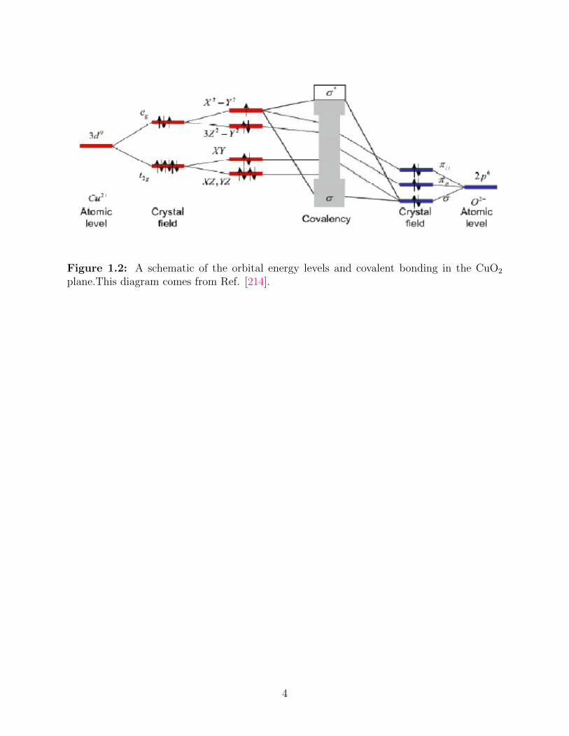
Figure 1.2: A schematic of the orbital energy levels and covalent bonding in the CuO2

plane.This diagram comes from Ref. [214].

4

a strong hybridization between them. The topmost partially filled band is the pd− σ∗ band

composed of the Cu 3dx2−y2 and O 2px,y orbitals.

A typical phase diagram of cuprate high-temperature superconductor is shown in the left

part of Fig. 1.3, in which the phase of zero dopant concentration is an antiferromagnetic

insulator (AF, the blue region), and the doped carriers destroy AF and lead to a

superconducting phase (red region). With increasing hole doping, the pseudogap appears,

in which conventional Fermi-Landu liquid theory fails to work and a superconducting gap

is opened. The pseudogap is not found in conventional superconductors. The optimal

hole concentration x is about 0.16, where Tc is maximum. In the overdoped region when

x > 0.16, the superconducting phase disappears and a “Normal” metallic phase appears. On

the electron doping side, there is no pseudogap and the superconducting phase penetrates

into the AF region. The phase diagram is not symmetric about x = 0.

1.1.2 Iron-based Superconductors

The iron-based superconductors mainly have five classes according to their structure: “1111”

type (LaFeAsO) [161],“122” type (AFe2As2) [222], “111” type (MFeAs) [257], “11” type

(FeSe) [102] and “32522” type (Sr3Sc2O5Fe2As2) [238](Fig. 1.4 (a)). Similar to the cuprates,

the iron-based superconductors have Fe-As layers and blocking layers alternatively stacking

along the c-axis. The blocking layers usually act as the insulating charge reservoir and the

Fe2As2 layer acts as the active conducting block. The Fe2As2 plane structure is shown in

Fig. 1.4 (b), where As atoms reside above and below this plane. The magnetic structure of

the Fe2As2 plane consists of ferromagnetic chains that are coupled antiferromagnetically in

the orthogonal direction [198].

Although the crystal structure of cuprates and FeSCs are similar that both are layer

structures, their electronic properties are very different. Most of the cuprates are octahedral,

while most of the FeSCs are tetrahedral at room temperature. Fig. 1.5 (b) shows that the t2g

orbitals (dxy, dxz, and dyz orbitals) have higher energy in the tetrahedral crystal structure and

are relevant to the conduction in FeSCs, while the higher energy orbitals eg (dx2−y2 and dz2

orbitals) are associated with conduction in cuprates. Also comparing the superconducting

phase diagrams of cuprates and iron pnictides (Fig. 1.3), two different things can be easily

5

Figure 1.3: The generalized temperature-filling phase diagram of the high-Tc cuprates (left)and iron-based superconductors (right). This diagram comes from Ref. [135].

6

Figure 1.4: Crystallographic and magnetic structures of the iron-based superocnductors.(a) The five tetragonal structures known to support supercoductivity. (b) Iron layerstructure. Iron ions are shown in red and pnictogen.chalcogen anions are shown in gold.(c) The magnetic structure in the iron layer. This diagram comes from Ref. [198].

7

Figure 1.5: (a) Tetraheral ligand field surrounding a central transition metal (green sphere).(b) Splitting of the degenerate d-orbitals (withoud a ligand field) due to an oactahedral ligandfield (left) and the tetraheral field (tight). This diagram comes from [8].

8

identified. There is no pseudogap in the iron pnictides and one additional phase, the nematic

phase [190, 255], is presented. The nematic phase sits below the structure phase transition

and above the antiferromagnetism transition. The nematic phase has been reported in

the 1111 [118] and 11 system [261], but in the 122 system, the structure phase transition

temperature coincides with the magnetic transition temperature. Although it was recently

reported that the nematic phase in BaFe2(As1−xPx)2 appears at a temperatures higher than

the structural/magnetic transition [119], it is still unknown whether the existence of nematic

phase is universal for each FeSCs.

Different from the cuprate, there are five d orbitals near the fermi surface in iron pnictides.

Fig. 1.6 shows the five 3d orbitals distribution near the Fermi surface, which is calculated via

a two-dimensional band model [81]. Around the Γ point, the 3d2z orbital contributes to the

two band ζz2 and ωz2 well below EF . There are two hole pockets at the Γ point, formed from

3dxz and 3dyz orbitals. The 3dxy orbital contributes to the electron pocket at the M point.

This electron pocket is also associated with 3dyz orbital along the x-axis and the 3dxz orbital

along the y-axis, respectively. The 3dx2−y2 orbital was found to be irrelevant to the low-

energy electronic structure. These results also consist with an angle-resolved photoemission

spectroscopy (ARPES) study in BaFe1.85Co0.15As2 [290] and generally true across the FeSCs.

1.1.3 Ba1−xKxBiO3 and BaPb1−xBiO3 superconductors

Pure BaBiO3 is insulating to well above 800 K and has a perovskite structure. At room

temperature, its crystal structure is a cubic lattice with Bi atoms siting at each corner and

O atoms linking each Bi pair (see Fig. 1.7). In the insulating state, the uniform crystal

structure is distorted and the BiO6 unit cell is tilted and consisted by two octahedron that

one is expanded and the other one is collapsed. Earlier, it was recognized that this insulating

phase comes from the charge order state comprised of Bi3+ and Bi5+ sites [50, 51, 204], and

the two octahedron correspond to the Bi3+ and Bi5+ oxidation states [110]. But experiments

have not observed distinct bismuth valences in BaBiO3 [89, 31, 267]. Some theories have

proposed the insulating state is induced by the attractive on-site interaction [217, 251] or

the negative charge transfer energy that holes reside on the oxygen ligands [182]. The origin

of the insulating state is still not clear now. A recent DFT calculation showed that the

9

Figure 1.6: A typical orbital assignment of bands of iron pnictide as calculated in Ref.[290]

10

Figure 1.7: (a) Sketch of the x-T phase diagram of Ba1−xKxBiO3. The space groups are:Mono. I=P21/n; Mono. II=I2/m; Rhomb.=R3; Cubic II=Fm3m. (b) Depiction of theinsulating ground state (x = 0) exhibiting breathing and tilting distortions. The collapsedand expanded BiO6 octahedra are shown in dark and light blue (gray), respectively. [207]

11

electronic band structure of BaBiO3 near the Fermi surface is dominated by the Bi 6s and O

2p states (see Fig. 1.8[207]). It was found that most of Bi 6s states contribute to dispersive

bands roughly 8 to 13 eV below the Fermi surface, while the O 2p states are located from

4 to 7 eV below the Fermi surface. This result consistent with the ARPES results [207]

and suggests that when hole doping ( i. e. K doping), most of holes occupy the O 2p

orbitals within the sublattice of collapsed BiO6 octahedra [73]. This result does not favor

the Bi3+Bi5+ charge order state, in which holes should reside on the Bi atom to destroy the

charge order.

In Pb or K-doped BaBiO3 with high values of superconducting transition temperature

are observed, which extended up to 13 K for Pb-doped alloys [11] and up to 30 K for K

alloys [173]. The superconductivity of Ba1−xKxBiO3 is observed with x values from about

0.30 to 0.45. The maximum Tc is 34 K occurs at x ≈ 0.35. The crystal structure in the

superconducting phase is tetragonal. The cubic-to-tetragonal transition is continuous. In

Ba1−xKxBiO3, with increasing x, holes are added to the parent system but without modifying

the underlying BiO lattice. While in BaPb1−xBixO3, the case is different. With increasing x,

not only are holes introduced but also Bi atoms are replaced by Pb atoms. Superconductivity

with narrow transition temperature is observed only close to x = 0.25 in BaPb1−xBixO3.

1.2 Correlations in High Tc superconductors

1.2.1 Cuprates

Electrons on 3d orbitals have a strong local Coulomb interaction U that prevents two

electrons to reside on a single site. Typically, the insulator driven by a strong local Coulomb

interaction (U t, t is the hopping integral) is called a Mott insulator. And the phase

related to the Mott insulator is called a Mott phase, which can be described by the Hubbard

model. It was found that the Mott transition in a single band Hubbard model is related

to the lattice geometry, dimension, and U . For example, on a one-dimensional chain, the

ground state for a half-filled band is insulating for any nonzero U [152]. On two-dimensional

square lattices the critical value for the Mott phase transition at half filling is Uc ∼ 4t[268];

12

Figure 1.8: Calculated total DOS (solid line), as well as the O 2p and bi 6s orbital-projectedDOS (short and long dashed lines, respectively.)[207]

13

but on two dimensional triangular lattices the phase transition boundary at hall filling is at

12t [7].

For the cuprates, the case is a little more complex. The hybridization between the Cu

3dx2−y2 and O 2px(y) electrons forms a bonding (B), nonbonding (NB), and antibonding

(AB) bands near the Fermi surface (see fig. 1.9 (a)). The bonding and nonbonding bands

are fully occupied and the antibonding band is half occupied. At half filling, the Hubbard

interaction splits the antibonding band into two bands (see fig. 1.9(b)): the upper Hubbard

band (UHB) and the lower Hubbard band (LHB). In the cuprates, the charge transfer

energy ∆ of moving one electron from oxygen atoms to the copper atom is smaller than

the onsite Coulomb repulsion U , which characterizes these compounds more precisely as

charge-transfer insulators (see fig. 1.9(c)) [284]. In the undoped cuprates, both the inverse

photoemission spectroscopy [77, 274] and optical conductivity [250, 49] measurements found

the charge transfer gap ∆ is about 1.5 eV. Also, an extended photoemission spectroscopy

study found that local Coulomb repulsion on the copper is about 12 eV in La2−xSrxCuO4 [237]

and Bi2Sr2CaCu2O8 [286]. All these results support that the cuprates are charge-transfer

insulators.

Therefore the cuprates should be described in terms of the three-band Hubbard model, in

which Cu 3dx2−y2 as well as O 2px and 2py orbitals are included [67, 251]. However, because

of the hybridization between the correlated Cu and the O orbitals, the first hole occupied

state correspond to the O-derived Zhang-Rice singlet band (see fig. 1.9(d)) [288]. It was

suggested that one can use an effective single-band Hubbard model to describe the cuprates.

In the effective single-band Hubbard model, the Zhang-Rice singlet band corresponds to the

lower Hubbard band, and the in-plane Cu-derived band is treated as the the upper Hubbard

band. These two bands are separated by an effective Mott gap ∆. The Hamiltonian is

written as

H = −t∑〈i,j〉,σ

(c†i,σcj,σ + h.c.

)+ U

∑i

ni,↑ni,↓, (1.1)

14

Figure 1.9: Density of states for opening a correlated gap. (a) the system is metallic in theabsence of electronic correlations, and becomes (b) a Mott insulator or (c) a charge-transferinsulator, respectively, for ∆ > W and U > ∆ > W . (f) due to the hybridization withthe upper Hubbard band, the nonbonding band further splits into triplet and Zhang-Ricesingle states. In the graph, B, AB, and NB represent bonding, antibonding, and nonbondingbands, respectively. This graphs comes from Ref. [58]

.

15

in which c†i,σ

(ci,σ

)creates (annihilates) an electron or hole on site i with spin σ, 〈i, j〉

represnets nearest-neighbor pairs, t is the hopping integral, and ni,σ = c†i,σci,σ is the number

operator.

In the strong-coupling limit (U t), the Hubbard Hamiltonian can simplify into the

t− J Hamiltonian [56], which is more commonly used in studying the low-lying excitations

of the half filled antiferromagnetic insulator

H = −t∑〈i,j〉,σ

(c†i,σ cj,σ + h.c.

)+ J

∑〈i,j〉

(Si · Sj −

ninj4

), (1.2)

where the operator ci,σ = ci,σ(1 − ni,−σ) excludes double occupancy, J = 4t2/U is the

antiferromagnetic exchange coupling constant, and Si is the spin operator for site i.

1.2.2 Iron-based superconductors

Many theoretical and experimental studies have shown that the electronic correlations in the

iron-based materials are not as strong as in the cuprates[273, 211]. A simple indication of

this is the absence of any Mott physics in the FeSCs: the parent compounds are all metallic

and there is no indication of nearby insulating behavior. Also x-ray absorption and inelastic

scattering measurements on SmFeAsO0.8, BaFe2As2, and LaFe2P2 show that their spectra

closely resemble that of elemental metallic Fe, suggesting Hubbard U . 2 eV and Hund’s

coupling strength J ∼ 0.8 eV [273].

Another key difference is that all 3d orbitals rather than a single 3dx2−y2 play essential

roles in electronic properties in FeSCs, which requires us to consider a multiorbital hubbard

model. The details of the multiorbital Hubbard model will be discussed in chapter 5.

Multiple d orbitals in FeSCs produces more diverse phenomena than that in cuprates, such

as Hund’s metals [79] and spin-freezing behavior [265]. Also, it was found that different 3d

orbitals in iron chalcogenides have different properties, which is called the orbital-selective

property [275, 282]. For example, the dxy orbital at Γ point is renormalized by a factor of

∼ 16, while dxz and dyz orbitals are only renormalized by a factor of ∼ 4 in FeTe0.56Fe1.72Se2

[275]. Moreover, an ARPES study showed that the spectral weight of the dxy orbital near

the Fermi surface disappears when warming FeTe0.56Se0.44, K0.76Fe1.72Se2, and FeSe film

16

grown on SrTiO3, which suggests that the orbital-selective Mott phase (OSMP) transition

occurs in iron chalcogenides as well [275, 276]. The OSMP refers to a phase in which a part of

orbitals is Mott insulating while the other orbitals are metallic. Fig. 1.10 shows a theoretical

simulation of the OSMP transition with different quasiparticle weight and orbital filling on

five 3d orbitals for the regular and 1/5-depleted iron selenides square lattices, respectively

[282]. The orbital-selective properties could be easily captured in fig. 1.10 and the Mott

phase transition firstly occurred on the dxy orbital, which coincides with experimental results.

In sum, the physics picture in the FeSCs is more complex than that in the cuprates and many

people argued that those multiple degrees of freedom, including orbital, charge, and spin,

play a significant role in high-temperature superconductors [65].

1.2.3 Ba1−xKxBiO3 and BaPb1−xBiO3 superconductors

Ba1−xKxBiO3 is nonmagnetic and a transition-metal-free superconductor. Due to the fact

that CDW and SC phases are presented in the phase diagram, a negative-U extended

Hubbard model is proposed to explain the pairing mechanism [217, 251, 183]. But the issue is

where does the negative U come from. Rice and his co-workers claimed the negative U arises

from the electron-phonon interactions [217]; however, Varma proposed that the negative U

occurs due to the nonlinear screening and the polarization of interatomic repulsion [251].

The nonlinear screening is that the energy of the 6s0 configuration is screened by the charge

transfer from the oxygen octahedra to the 6p shell, which prefers double occupations on a Bi

site. If the negative U has an electronic origin, the semiconducting phase of these materials

is unique, because charge ±2e bosonic bound states of two electrons or two holes dominate

its transport properties. The electronic origin explains the two different gaps observed in

the optical and transport experiments (2 and 0.24 eV, respectively) that in the optical

experiments the excitation is two-particle excitation, while in the transport experiments

the excitation is single particle excitation [246, 247]. But the superconducting transition

temperature and the coherence length produced by the electronic origin are much higher

and lower than results from experiments, respectively. Instead, if the phonon mechanism is

employed, it is easy to get a reasonable numbers for the transition temperatures [246]. Later,

photoemission and x-ray absorption experiments showed that the two gaps 2 eV and 0.24

17

Figure 1.10: (a), (b) The regular and 1/5-depleted square lattices, respectively,corresponding to the alkaline iron selenides with disordered and

√5 ×√

5 ordered ironvacancies. (c) and (d) shows the evolution of orbital resolved quasiparticle spectral weightZα and orbital filling factor (per iron site per spin) with U for the multiorbital model onlattices (a) and (b), respectively. This graphs is cited from Ref. [282]

.

18

eV in fact correspond to the direct and indirect energy gaps [124, 191]. This result is against

the electronic origin. However, the problem of the phonon mechanism is that the electron-

phonon coupling calculated by the standard DFT, LDA, or GGA approach is insufficient to

account for the high Tc in Ba1−xKxBiO3. This issue is addressed by introducing correlation

effects in the standard DFT [74, 279]. It is found that the strong electronic correlations

can enhance the e-ph coupling and estimated the realistic e-ph coupling λ ∼ 1.0 for optimal

hole doped BaBiO3, which is large enough to explain the high Tc in K-doped BaBiO3 [279].

However, Plumb et. al. compared band structures of BaBiO3 from the standard DFT

calculation and the angle-resolved photoemission spectroscopy (ARPES) experiment, and

found that both band structures are consistent with each other [207]. This result indicates

the electron correlations in BaBiO3 is weak. If this conclution is correct, to support the

phonon mechanism, the community needs to figure out to answer a question that how a

small e-ph coupling can lead to a high Tc.

1.3 Evidence for the Electron-Phonon Interactions in high-TC

superconductors

1.3.1 the Cuprates

Many people believe the e-e interaction plays a key role in superconductivity in the cuprates

and the e-ph interaction is negligible [12, 30, 87]. But this idea seems too premature in

light of several experimental studies. For example, in different hole-doped cuprate materials,

two kinks are observed in the electronic dispersion along the nodal and antinodal directions,

respectively, using ARPES [136, 54]. A common sense is that these kinks are induced by

the electron-boson coupling, but the question is whether the boson is the magnon or the

phonon. This issue can be addressed considering that both kinks exist above and below Tc

[54], suggesting the boson should not be the spin response mode, which only observed in

certain materials and only below Tc. Moreover, it is suggested the nodal kink is induced

by the half-breathing mode based on neutron experiments [206] and the antinodal kink is

induced by the 40 meV B1g oxygen ”bond-buckling” phonon [54, 60, 142]. Both kinks are

also observed in electron-doped cuprate superconductors and are likely induced by the half-

19

and full breathing mode phonons, respectively [201]. The evidence to support phonon is that

in the electron-doped cuprate superconductors, neutron experiments showed that the energy

of the spin resonance mode is at most 10 meV [270], which is much smaller than the energies

of the nodal and antinodal kinks and the spin resonance mode could not be responsible for

both kinks.

The importance of the phonon is also corroborated in inelastic neutron-scattering

experiments and inelastic X-ray scattering, which showed the bond-stretching phonon

anomaly in La2−xSrxCuO4 and YBa2Cu3O0.95. [215, 216, 245]. This anomaly occurs at a

wave vector corresponding to the charge order and is associated with charge inhomogeneity

in cuprate superconductors.

Many people argue that the e-ph coupling cannot support the d-wave symmetry pairing

in the cuprate superconductors, but the aforementioned facts imply that the e-ph coupling

may be important to our understanding of superconductivity, although its contribution is

likely to be indirect [114]. This indicates the e-ph coupling remains necessary to be studied

in the correlated system.

Usually, there are two types of the e-ph couplings. The first one is via a deformation

coupling where the atomic vibration modulates the overlap of the atomic orbitals of

neighboring atoms. One famous theoretical model to capture this coupling is the Su-Shrieff-

Heeger model [243], which has been widely used to study in organic materials [146]. This

type of coupling is relevant to the half- and full breathing modes in the cuprates [60], which

will be discussed in detail in chapter 6. The second one is the electrostatic coupling. This

occurs when the lattice site oscillates through a local crystal field arising from an asymmetry

in the local crystal environment. In this case, the e-ph coupling modulates the onsite energy

of the atomic orbitals and can be described by the Holstein model, which is written as

H = −t∑〈i,j〉,σ

(c†i,σcj,σ + h.c.

)+∑i

(p2i

2M+Kx2

i

2

)+ g

∑i,σ

xini,σ. (1.3)

Here, c†i,σ (ci,σ) is the electron creation operator, and xi and pi are the atoms’ displacement

and momentum operators, respectively. The last term of the Hamiltonian describes the

20

charge transfer e-ph coupling. In the cuprates, the coupling to the c-axis modes is largely of

this type [61].

1.3.2 the FeSCs

Similar to the cuprates, the electron-phonon (e-ph) interaction was considered as a secondary

interaction in FeSCs since a first principle study found the e-ph coupling constant in LaFeAsO

is only λ = 0.21, which is not enough to produce high Tc [26]. This calculation is based on

the paramagnetic phase, which is not the case for the parent compounds of FeSCs. It

is suggested that the e-ph coupling through the spin channel is relevant in Fe pnictides,

since the lattice is intimately involved in magnetism such as the Invar effect [66]. Later,

DFT studies showed that the e-ph interaction is enhanced by the magnetism up to λ .

0.35 [280, 25, 48], which is still not enough to explain the high superconducting critical

temperature but is strong enough to have a non-negligible effect on superconductivity and

other properties. In experiments, infrared spectroscopy studies find an unusual redshift of

the Eu mode in the K-doped BaFe2As2 [271] as well as the asymmetry line shape of the

optical conductivity near the Eu mode [271, 101], suggesting the coupling between lattice

vibrations and other channels, such as charge or spin. Recently, femtosecond time- and

angle-resolved photoemission spectroscopy (trAPRES) and time-resolved x-ray diffraction

(trXRD) measurements were performed to record the deformation energy induced by the

A1g phonon in FeSe [224]. It is found that the e-ph coupling strength is about ten times

as estimated in Ref. [26], which could be captured in DMFT+LDA calculations. All these

results highlight that phonons play an important role in shaping electronic properties in bulk

FeSCs materials.

In addition, phonons become more pronounced at interfaces. Recently, it was discovered

a dramatic enhancement of the superconducting transition temperature in FeSe, from 8 K in

bulk [102] to nearly 70 K [141] when grown as a single unit cell layer on SrTiO3 substrates.

One suggested that this enhancement comes from the forward phonon scattering between

the FeSe film and the substrate [141, 138, 258, 259, 213]. Also, some studies claimed that the

substrate allows an antiferromagnetic ground state of FeSe and opens e-ph coupling channels

within the monolayer[47]. In sum, the e-ph interaction cannot be neglected a priori in FeSCs.

21

1.3.3 Ba1−xKxBiO3 and BaPbxBiO3 superconductors

The importance of e-ph interactions in Ba1−xKxBiO3 has been revealed by many experiment

studies and has been postulated in many theoretical works. For example, the oxygen-

isotope effect is prominent in Ba1−xKxBiO3 [13, 158, 94]. For a BCS superconductors,

isotopic substitution of a particular atomic species will affect the superconducting transition

temperature as well as the phonon spectrum. By measuring Tc between a 100% 16O sample

and a 65% 18O exchanged sample of Ba0.6K0.4BiO3, it was found the Tc obeys Tc ∼ M−αOO ,

where MO is the mass of the oxygen isotope and αO = 0.22 ± 0.03 [13]. Also, the e-ph

coupling is confirmed in the Tunneling spectroscopy measurements and it was found clear

evidence of phonon images in tunneling conductance up to 60 meV [287, 103] and the e-ph

coupling constant λ ∼ 1 [94]. This large e-ph coupling constant is confirmed by specific heat

experiments as well [130].

Although it was proposed that the nonlinear screening can induce the negative-U in the

Hubbard model, the detailed numerical calculations are not available. Moreover, it was

found the effective Hubbard U is always positive in the five-orbital model, including Bi s

and p, and O pσ orbitals, in the four-orbital model, including Bi s and O pσ orbitals, and in

an effective one band model using the constrained density-functional theory [253]. There is

no indication of a negative U arising from the electronic origin.

1.3.4 Nonlinear electron-phonon coupling

The electron-phonon coupling is one of the factors determining the stability of cooperative

order in solids, such as the superconductivity, charge, and spin density waves. In the pump-

probe experiments, the transient lattice displacement driven by the optical photons could be

large, implicating the nonlinear e-ph coupling needed to be considered. Therefore, the ability

of controlling the e-ph coupling strength by optical driving may open up new possibilities

to steer materials’ functionalities. For example, the nonlinear e-ph coupling of Raman-

active modes has been widely studied in MgB2 and is treated as a key factor to explain

the observed high TC and boron isotope effect in MgB2 [277]. Also, both terahertz time-

domain spectroscopy (THZ TDS) and time- and angle-resolved photoemission spectroscopy

22

(tr-ARPES) experiments showed a transient threefold enhancement of the e-ph coupling

constant in SiC [208], which is likely due to the nonlinear e-ph coupling [235]. But another tr-

ARPES experiment showed the transient electron-boson interaction is reduced in a cuprate

superconductor [289]. The suppression of the electron-boson coupling may be due to the

interplay between the nonlinear e-ph interaction and the Coulomb interaction. However,

it remains unclear how the nonlinear e-ph coupling corporate/compete with the linear e-

ph coupling and the Coulomb interaction in solid materials [120]. In the chapter 3, I will

answer a part of this question and explain the interplay between the nonlinear and linear

e-ph couplings and study its effect on the superconductivity and the CDW phase.

1.4 Scope and Organization

The goal of this thesis is to examine the role of e-ph interactions in multiorbital strongly

correlated systems using numerical techniques. The overall organization is as follows.

Chapter 1 (this chapter) focus on introducing e-e correlations and e-ph interactions in high-

temperature superconductors, including cuprates, FeSCs, and Ba1−xKxBiO3. The effective

Hubbard model for the cuprates and the Holstein model, in which the onsite energy of the

atomic orbitals is modulated by the lattice vibration, are introduced as well in this chapter.

Chapter 2 introduces two numerical techniques used to solve the Hamiltonian relevance

to phonons and correlated electrons. The first one is the determinant quantum monte carlo

(DQMC) and the second one is the dynamical mean field theory (DMFT). I will use the

Hubbard model to illustrate how these two techniques work.

In chapter 3 I will study the role of the nonlinear e-ph coupling in an modified Holstein

model. Here, the e-e interaction is not included in this model. My starting point is to

understand the interplay between the nonlinear and linear e-ph couplings absence of the

Coulomb interaction. The influence of the Coulomb interaction will be considered in my

future research.

In chapter 4 I will examine the momentum dependence of the orbital-selective behavior

in a three-orbital Hubbard model. It will be shown that itinerant electrons in the OSMP

have strong momentum dependence while the localized electrons are almost momentum

23

independent. This study also paves a way to further examine the role of the e-ph interaction

in the OSMP.

In chapters 5 I will study the influence of the e-ph interaction on the orbital-selective

behavior in a multiorbital Hubbard-Holstein model. This work will be done in both infinite-

and one-dimensions using DMFT and DQMC, respectively. It will show that a weak to

intermediate e-ph coupling can strongly modified the phase diagram both in a 1D system

and an infinite dimension system. It is hopefully to extend my conclusion to two and three

dimensions, where the cuprates and FeSCs is relevant.

In chapter 6 I will study the breathing phonon in superconductors Ba1−xKxBiO3. I will

show how the nonlocal e-ph coupling produces a dimerized structure and how this structure

disappears as doping. Also, I will study the localization of polarons and bipolarons in the

metal-to-insulator transition. The superconducting state induced by the breathing phonon

will examined as well.

Finally, in chapter 7, conclusions will be presented as well as discussion of possible

extensions of this work in the future.

24

Chapter 2

Methodology

Most of the strongly correlated many body problems cannot be solved in analytically. One

simple model for the correlated systems is the Hubbard model. In this chapter, I will present

two numerical methods to solve the Hubbard model. The first method is the determinant

quantum Monte Carlo, which allows to treat e-e and e-ph interactions exactly. The second

one is the dynamical mean field theory, which neglects spatial correlations. The application

of the determinant quantum Monte Carlo to the Holstein model is also discussed in this

chapter.

2.1 Hubbard model

The Hubbard model was originally proposed to describe the ferromagnetism in transition

metals [104]. The Hamiltonian includes the electron hopping and onsite electron-electron

interaction terms and is written as

H = −∑〈i,j〉,σ

ti,jc†i,σcj,σ +

∑i

Uni,↑ni,↓ − µ∑i

ni,↑ni,↓, (2.1)

in which c†i,σ creates an electron with spin σ on site i, tij is the hopping integral, U is the

onsite Coulomb repulsion strength, and µ is the chemical potential used to fix the charge

density. The Hubbard model describes an interacting many-body system which cannot be

solved analytically, except in dimension d = 1 with nearest-neighbor hopping [152]. To study

25

correlation phenomena such as the Mott transition in higher dimensions, both dynamical

mean field theory (DMFT) [78, 166] and Quantum Monte Carlo (QMC) methods have been

widely applied.

To better understand the Hubbard model, I will discuss the solution of the single site

case, which is the simplest case. In the single site limit, the electron Green’s function at the

imaginary time τ is

G(τ) = −〈Tτc↑(τ)c†↓(0)〉

= − eµτ + eβµeτ(µ−U)

1 + 2eβµ + eβ(2µ−U), (2.2)

where β is the reciprocal of the thermodynamic temperature. The Green’s function in the

Matsubara frequency space is

G(iωn) =

∫ β

0

dτG(τ)eiωnτ

=1

1 + 2eβµ + eβ(2µ−U)

[eµβ + 1

µ+ iωn+e(2µ−U)β + eµβ

µ− U + iωn

]. (2.3)

The spectral function is obtained via

−G(τ) =

∫ ∞−∞

A(ω)e−ωτ

1 + e−βωdω, (2.4)

in which

A(ω) =1 + eβµ

1 + 2eβµ + eβ(2µ−U)δ (ω + µ) +

eβµ + eβ(2µ−U)

1 + 2eβµ + eβ(2µ−U)δ (ω + µ− U) . (2.5)

Equation 2.5 shows that there are two δ functions in the spectral functions. These two δ

functions are separated by a Mott gap with a scale of U . On the cluster, these two δ functions

are expanded to continuous functions.

26

2.2 Determinant Quantum Monte Carlo Method

Solving the Hubbard model on the cluster remains a big challenge to date. Determinant

quantum Monte Carlo is one of the ways to solve the Hubbard model exactly. DQMC is

an auxiliary field imaginary-time Monte Carlo method for simulating interacting systems of

particles in the grand canonical ensemble [24, 231, 269]. In the following, I will discuss the

application of DQMC in solving the Hubbard model.

2.2.1 The General Methodology

First I divide the Hubbard model into two parts, H = K + V , where

K = −t∑i,σ

(c†i,σci+1,σ + h.c.)− µ∑i

(ni,↑ + ni↓), (2.6)

V = U∑i

ni↑ni↓ (2.7)

Here, K is the non-interacting Hamiltonian and V is the Hubbard interaction. In DQMC, the

major task is to calculate the partition function Z ≡ Tre−βH . One way to obtain the partition

function is dividing the inverse temperature interval [0, β] into many small imaginary time

slices ∆τ = β/L (L is the number of time slices). Then the partition function can be written

as

Z ≡ Tre−βH

= Tre−∆τLH

= Tr[e−∆τV e−∆τK

]L+O

(∆τ 2

)≈ Tr

∏l

[e−∆τV e−∆τK

]. (2.8)

In the Eq. (2.8) the Trotter approximation is applied [269, 76]. ∆τ is a controllable error,

and when ∆τ is small enough, this approximation is reasonable. The Hubbard interaction

term can be reduced into quadratic terms by introducing an auxiliary field si,l = ±1 at each

27

site and time slice and applying a discrete Hubbard-Stratonovich transformation [95]

e−αni,↑ni,↓ =

12eα/2(ni,↑+ni,↓)

∑si,l=±1 e

−λsi,l(ni,↑−ni,↓) (α > 0)

12eα/2(ni,↑+ni,↓)

∑si,l=±1 e

−λsi,l(ni,↑+ni,↓−1)+α2 (α < 0)

, (2.9)

where λ = ln(e|α|/2 +√e|α| − 1). In the single band Hubbard model α = ∆τU > 0. Then

the partition function can be written as

Z = Tr∏l

[e−∆τV (l)e−∆τK

]= Tr

∏l

∏

i

1

2eα/2(ni,↑+ni,↓)

∑si,l=±1

e−λsi,l(ni,↑−ni,↓)

e−∆τK

. (2.10)

The term eα/2(ni,↑+ni,↓) can be absorbed into the chemical potential by changing K to K ′ =

K +∑i

U2

(ni,↑ + ni,↓). If I define matrices

B↑(↓)l = e−(+)

∑i λsi,lni,↑(↓)e−∆τK′ , (2.11)

the partition function becomes

Z = Tr∏l

(∑si,l

B↑l B↓l )

=∑si,l±1

Tr(B↑LB↑L−1...B

↑1)Tr(B↓LB

↓L−1...B

↓1). (2.12)

In order to calculate the partition function, I use the following relationship [24]

Tr(ec†T1c ec

†T2c ...ec†Tnc

)= det

(I + eT1eT2 ...eTn

), (2.13)

where c† =[c†1, c

†2, . . . , c

†N

]is a row vector and I is a N × N identity matrix (N is the size

of the system). Tm is an arbitrary symmetric matrix. Then the partition function is

Z =∑

si,l=±1

det(I +B↑LB

↑L−1...B

↑1

)det(I +B↓LB

↓L−1...B

↓1

)

28

=∑

si,l=±1

det(M↑) det

(M↓) , (2.14)

in which M↑(↓) = I +B↑(↓)L B

↑(↓)L−1...B

↑(↓)1 .

The thermodynamic expectation value of any observable O at finite temperature is defined

by

〈O〉 =Tr(Oe−βH

)Z

. (2.15)

Most observables can be expressed in terms of the single particle Green’s function. The equal

time Green’s function Gσij(l) at a discrete time τ = l∆τ and at a displacement d = ri − rj

for an electron propagating through the field produced by the si,l is given by [269]

Gσij(l) = 〈Tτ [ci,σ(τ)c†j,σ(τ)]〉

= [I +Bσl ...B

σ1B

σL...B

σl+1]−1

ij

= M−1i,j . (2.16)

To evaluate 〈O〉, Eqs. 2.14 and 2.15 show that I need to do a summation over all si,l

configurations. However, it is impossible to go through all si,l configurations in numerical

calculations. To overcome this issue, I use the importance sampling method in the Monte

Carlo. Here, the importance sampling generates a sequence of Hubbard-Stratonovich (HS)

configurations si,l, with a distribution probability p (si,l) = detM↑detM↓

Z. In the Monte

Carlo, the transition probability W(si,l → s′i,l

)decides how to accept an update. The

relationship between the transition probability and the distribution probability is given by

a detailed balance condition

W(si,l → s′i,l

)× p (si,l) = W

(s′i,l → si,l

)× p

(s′i,l

). (2.17)

Then I have

W(si,l → s′i,l

)W(s′i,l → si,l

) =p(s′i,l

)p (si,l)

≡ R. (2.18)

29

In the Monte Carlo, I can only obtainR rather thanW(si,l → s′i,l

)andW

(s′i,l → si,l

).

The specified value of W(si,l → s′i,l

)is not given in Eq. (2.18). But I can choose any

W(si,l → s′i,l

)once it satisfy Eq. (2.18). One typical solution is the Metropolis-Hastings

algorithm [91, 18]. Here, I use the heat bath method [53], which is given by

W(si,l → s′i,l

)=

RR+c

R > 1

R1+c×R R ≤ 1

, (2.19)

where c is adjusted in our code to maintain a certain acceptance rate.

In the determinant quantum Monte Carlo, I first set the initial HS field for each time

slice and site and then flip the HS field at one site and time slice. The ratio of determinants

after and before flipping is

R = R↑R↓ =detM ′↑detM ′↓

detM↑detM↓ . (2.20)

in which M ′σ is a new M matrix after flipping a field si,l → −si,l. There is an efficient

algorithm for calculating Rσ [269, 115], that is

Rσ =detM ′σ

detMσ= 1 + [1−Gσ

ii(l)]∆σii(i, l), (2.21)

in which ∆↑,↓jk (i, l) = δjiδki[e±2∆τsi,l−1]. For each flip, the transition probability is calculated

via Eq. (2.19) and compared to a random number r. Once W(si,l → s′i,l

)> r I accept

this field flipping with a new Green’s function

G′σ(l) = Gσ(l)− Gσ(l)∆σ(i, l)[1−Gσ(l)]

1 + [1−Gσii(l)]∆

σii(i, l)

. (2.22)

After all sites on a given time slice have been updated, I advance to the next time slice. The

Green’s function for the next slice is given by

Gσ(l + 1) = Bσl+1G

σ(l)[Bσl+1]−1. (2.23)

30

In DQMC I first set a large number of updating steps for warming up in that the HS fields

should be updated close to the thermal equilibrium configurations before any measurement

is applied.

2.2.2 Unequal Time Green’s Function

Green’s function G(ri, τl; rj, τl′) is a function of ri − rj and τl − τl′ . When τl = τl′ = l∆τ ,

Green’s function G(ri, τl; rj, τl′) becomes equal time Green’s function Gij(l). The equal time

Green’s function can be calculated via Eq. (2.16). However, in order to measure dynamic

quantities, one needs to measure the unequal time Green’s function (τl 6= τl′), which can be

obtained by [115]

G(τl, τl′) =

G(l′) [B(l − 1) · · ·B(l′)] (τl > τl′)

−G(l′) [B(l − 1) · · ·B(1)B(L) · · ·B(l′)] (τl < τl′)(2.24)

2.2.3 Measurements and Error Estimates

The average value of an observable O defined in Eq. (2.15) is obtained by

〈O〉 =1

M

M∑k=1

〈O〉k, (2.25)

where M is the number of measurements, 〈O〉k is the result at a given field configuration

si,l. The sample variance is defined by

s2 =1

M − 1

M∑k=1

[〈O〉k − 〈O〉]2, (2.26)

Many physical observables can be evaluated by the Green’s function. For example, the

charge density ni,σ of spin σ on the site i is obtained by

〈nσ,i〉 =1

L

L−1∑l=0

[1−Gσii(l)] . (2.27)

31

The double occupancy on site i is given by

〈ni,↑ni,↓〉 =1

L

L−1∑l=0

(1−G↑ii(l)

)(1−G↓ii(l)

), (2.28)

and the local moment on site i is

〈(ni,↑ − ni,↓)2〉 = 〈ni,↑ + ni,↓〉 − 2〈ni,↑ni,↓〉

=1

L

L−1∑l=0

[(2−G↑ii(l)−G

↓ii(l)

)− 2

(1−G↑ii(l)

)(1−G↓ii(l)

)]. (2.29)

Correlation functions can be expressed in terms of Gσ(τ) through application of the Wick

theorem as well [165]. For example, the charge-density-correlation function χCDW is defined

as [230, 172]

χCDW(q) =1

N

∫ β

0

dτ〈ρq(τ)ρ†q(0)〉

=1

N

∑ri,rj ,σ,σ′

e−iq·(ri−rj)∫ β

0

dτ〈nri,σ(τ)nrj ,σ′(0)〉 (2.30)

in which ρq(τ) =∑

ri,σe−iq·rinri,σ(τ), nri,σ = c†ri,σ(τ)cri,σ(τ), and N is the total cluster size.

Following Wick theorem, 〈nri,σ(τ)nrj ,σ′(0)〉 is calculated by

〈nri,σ(τ)nrj ,σ′(0)〉 =

〈nri,σ(0)〉 ri = rj, σ = σ′, τ = 0

〈nri,σ(τ)〉〈nrj ,σ′(0)〉 σ 6= σ′

〈nri,σ(τ)〉〈nrj ,σ(0)〉−

Gσ(rj − ri,−τ)Gσ(ri − rj, τ) σ = σ′

.

The magnetic correlations χS(q) is given by [269, 95]

χS(q) =1

N

∑ri,rj

eiq·(ri−rj)∫ β

0

dτ⟨[nri,↑(τ)− nri,↓(τ)]

[nrj ,↑(0)− nrj ,↓(0)

]⟩. (2.31)

32

For conventional superconductors, the gap has s-wave symmetry; while for cuprates, the

gap has d-wave symmetry. The different gap symmetries lead to different formulas for pair-

field or superconducting susceptibilities. For completeness, a general formula for these two

kinds of gaps with only onsite and nearest neighbor correlations is [269, 230, 172]

χSC =1

N

∫ β

0

dτ〈∆ (τ)∆†(0)〉, (2.32)

where

∆†(τ) =

∑

i c†i,↑c†i,↓ s−wave

12

∑i,δ Pδc

†i,↑c†i+δ,↓ d−wave

. (2.33)

Here, δ is an index that runs over nearest neighbors of the site i and the phase factor Pδ

alternates in sign with P±x = 1 = −P±y. To distinguish the two gap symmetries, the

pair-field susceptibilities will be denoted χs and χd for the s- and d- wave case, respectively.

2.2.4 The Fermion Sign Problem

In general, the factor det(M↑)det(M↓) is not positive due to Fermi statistics. When I apply

an operator c†j,σ to a many-body wave function |ψ〉, a phase factor ±1 is determined by

the order of the creation operators c†i,σ applied to the vacuum state to produce |ψ〉. But

I don’t know this order in my DQMC calculations, which results in a negative value of

det(M↑)det(M↓) for some configurations. This negative problem is called the Fermion sign

problem. To overcome it the absolute value of the product |det(M↑)det(M↓)| is used and

the expectation value of an observable must be augmented by

〈O〉 =〈OPs〉〈Ps〉

, (2.34)

where Ps denotes the sign of the product det(M↑)det(M↓). The average sign depends on

a number of factors including the size of the system, the overall filling, the strength of the

interaction U , and inverse temperature β [157, 105]. At low temperature, the sign problem

becomes terrible and the average sign value tends toward zero for the Hubbard model at

33

non-half fillings due to particle-hole asymmetry. When the average sign value close zero, the

observable obtained from Eq. 2.34 becomes a meaningless large value.

2.3 Dynamical Mean Field Theory

2.3.1 Fermions in infinite dimensions

The DMFT maps a lattice problem with many degrees of freedom onto an effective single-

site problem with fewer degrees of freedom. More specifically, instead of studying the lattice

problem, DMFT extracts a local site on the cluster and using bath levels to effective describte

the hybridization on the cluster. At the same time, DMFT keeps all local interaction on this

local site. Results from DMFT are quanlitive correct for high dimensions and become exact

in the limit of infinite dimensions (d→∞) [78, 84].

Before talking about the DMFT technique, it is necessaty to rescale the Hubbard

Hamiltonian to ensure that in the d→∞ limit the energy per lattice site does not diverge.

The on-site Coulomb interaction term is not sensitive to the dimensionality and U can be

the same. The total kinetic energy in the mean field approximation with nearest-neighbour

hopping t is HKE =∫dερ(ε)t, and the density of states for the hyper-cubic lattice is

ρ(ε) =∫

ddk(2π)d

δ(ε− εk), in which εk = −2t∑d

i=1 cos(ki). In the infinity dimension (d→∞),

the bandwidth diverges and so do the density of states and kinetic energy. The proper scaling

is determined from the density of states for d→∞. One way to obtain the density of states

for d→∞ uses the Fourier transform of ρ(ε), which factorizes:

Φ(s) =

∫ ∞−∞

dεeisερ(ε) =

∫ddk

(2π)deisεk

=

[∫ π

−π

dk

2πexp

(−2ist∗√

sdcos(k)

)]d= J0

(2t∗√2d

)d=

[1− t2∗s

2

2d+O

(1

d2

)]2

= exp

[−t

2∗s

2

2+O

(1

d

)], (2.35)

where J0(z) is a Bessel function and t = t∗/√

2d. Then the density of states is

ρ(ε) =

∫ ∞−∞

dε

2πe−isεΦ(s) =

1

2π | t∗ |exp

[− ε2

2t2∗

]. (2.36)

34

When t∗ is constant, the kinetic energy becomes finite. Hence, on the hypercubic lattice, the

nearest-neighbor hopping t must be scaled proportional to 1/√

2d to obtain a meaningful

finite limit. In general, the n-th nearest neighbor hopping amplitude tn must be scaled

proportional to 1/√Zn, where Zn is the number of sites connected by tn. On the Bethe

lattice with infinite nearest neighbors Z (Z →∞), the nearest-neighbor hopping t = t∗/√Z

and the density of states has a semi-elliptic form ρ(ε) =

√4t2∗−ε22πt2∗

[64].

2.3.2 Detailed procedures

DMFT extracts one local site in the Hubbard model and treats it as an impurity site in the

Anderson impurity model (see Fig, 2.1). Here, the interaction bewteen the impurity site and

energy baths is effectively equal the interaction between this site and other sites in a lattice

model.

The Hamiltonian of the Anderson model is read as

HAIM =∑pσ

εpa†pσapσ +

∑pσ

(Vpc†σapσ + h.c.) + Un↑n↓ − µ(n↑ + n↓), (2.37)

where a†pσ creates an electron with spin σ on the bath p, c†σ creates an electron with spin

σ on the impurity site, and n = c†σcσ. The last term of Eq. (2.37) is introduced since this

Hamiltonian will be solved in the canonical ensemble and the chemical potential is used to

fixe the particle filling.

The Green’s function of the impurity site is defined as

G(iωn) =1

iωn + µ− Γ(iωn)− Σ(iωn), (2.38)

where ωn is the Mastubara frequency ωn = 2(n+ 1)π/β, β is the inverse of the temperature,

Σ(iωn) is the self-energy, and Γ(iωn) is the hybridization function and is defined as

Γ(iωn) =∑p

| Vp |2

iωn − εp. (2.39)

35

Figure 2.1: DMFT extracts one site from lattices and keeps local interactions on this site.At the same time, this site is coupled to energy baths.

36

The local Green’s function of the Hubbard model is written as

Gloc(iωn) =1

N

∑k

1

iωn − ξk − µ− Σ(k, iωn), (2.40)

where ξk is the eigenenergy of the kinetic energy of Eq. (2.1) and k is the momentum. In

the dynamical mean field approximation, I assume the self-energy Σ(k, iωn) is mometum

independent and labelled as Σloc(iωn). The local hybridization function of the Hubbard

model is obtained by

Γloc(iωn) = iωn + µ+ Σloc(iωn)−G−1loc(iωn). (2.41)

In the DMFT, I first give an initial value to Σloc(iωn) and calculate the local hybridization

function Γloc(iωn) via Eq. (2.41). This local hybridizarion function should equal Γ(iωn) in

that the hybridization to the bath is used to describe the hybridization between a local

site and other sites in the Hubbard model. The parameters Vp and ξp in Eq. (2.37) are

determined via Eq. (2.39) using the least squares minimization. Here, this fitting process is

done using the open-source MINPACK library. Solving the Anderson Impurity Hamiltonian,

I can get the impurity Green’s function G(iωn) and self-energy Σ(iωn). The DMFT requires

the impurity self-energy Σ(iωn) equal the local self-energy Σloc(iωn). For clarity, the whole

DMFT procedure is shown in Fig. 2.2. The iteration continues until a self-consistent solution

(Σ) is reached.

2.3.3 Impurity solver: Exact Diagonalization

In this thesis, I use the exact diagonalization to solve the Anderson impurity Hamiltonian

[155]. Assuming that I study the Anderson impurity Hamiltonian on a cluster with N − 1

bath sites and one impurity site, I have two possible states for each site: spin up and

spin down. Thus the system has 2N states, and this is the dimension of the Hamiltonian

matrix. The basis states in the charge number representations are |n1, n2, n3, · · · , nN〉↑ ⊗

|m1,m2,m3, · · · ,mN〉↓, where ni is the charge number on site i with spin up and mi is the

charge number on site i with spin down. For fermions, ni and mi can only be 0 or 1. The

37

Figure 2.2: DMFT self-consistent loop.

38

2N states can be enumerated as

|φ1〉 = |0, 0, 0, · · · , 0, 0〉↑ ⊗ |0, 0, 0, · · · , 0〉↓,

|φ2〉 = |1, 0, 0, · · · , 0, 0〉↑ ⊗ |0, 0, 0, · · · , 0〉↓,

|φ3〉 = |0, 1, 0, · · · , 0, 0〉↑ ⊗ |0, 0, 0, · · · , 0〉↓,...

|φ2N 〉 = |1, 1, 1, · · · , 1, 1〉↑ ⊗ |1, 1, 1, · · · , 1, 〉↓. (2.42)

The Anderson impurity Hamiltonian matrix is computed via

Hij = 〈ψi|H|ψj〉. (2.43)

For example, assume there are one impurity site and two bath levels. In the basis, I set the

first site as the impurity site and the other two sites corresponding to the bath 1 and bath

2. Here, I take the two basis states as

|φi〉 = |1, 1, 0〉↑ ⊗ |1, 0, 0〉↓,

|φj〉 = |1, 1, 0〉↑ ⊗ |1, 0, 0〉↓.

Calculating Hij one term by one term, I have

〈φi|2∑p=1

∑σ

εpa†pσapσ|φj〉 = ε1,

〈φi|2∑p=1

∑σ

(Vpc†pσapσ + h.c.

)|φj〉 = 0,

〈φi|Un↑n↓|φj〉 = U,

〈φi| − µ (n↑ + n↓) |φj〉 = −2µ.

Then the Hamiltonian matrix element is ε1 + U − 2µ.

A big issue of the exact diagonalization is that the Hamiltonian matrix size grows

exponentially with increasing N , making even small lattices of typically 10 sites difficult

39

to handle with standard diagonalization techniques. To make the Hamiltonian matrix size

accessible to the available computing power, I can reduce the matrix size by using

[H,S2] = [H,Sz] = [N ,H] = 0, (2.44)

where H is the Hamiltonian, S2 is the total spin number, Sz is the total spin in the z

direction, and N is number operator. This equation tells that S2, Sz, N are good quantum

numbers, and I can divide the 2N states into (N + 1)2 subspaces with each subspace has a

fixed number of particles and a fixed number of Sz. For example, in the subspace (n,m),

there are

N

n

× N

m

basis elements. For N = 10, the size of the largest subspace is

63,504, which is much smaller than 220 = 1, 048, 576. Hence, when the Hamiltonian matrix

is constructed in the subspace, it is much easier to diagonalize this small matrix.

2.3.4 Green’s function

After doing the exact diagonalization, I can get the eigenenergy En and eigenstate |φn〉. The

Green’s function is calculated using these eigenvalues via

G(ri, rj, iωn) =1

Z

∑n,m

e−βEn + e−βEm

iωn + Em − En〈φm|ci |φn〉〈φn|c

†j|φm〉

=1

Z

∑m

e−βEm∑n

[〈φm|ci |φn〉〈φn|c

†j|φm〉

iωn + Em − En+〈φm|c†j|φn〉〈φn|ci |φm〉iωn + En − Em

].

(2.45)

There are two summations appearing in the expansion for the Green’s function, and if the

space of the basis is large, it will take a long time to calculate this Green’s function. To

reduce the time, I use a Lanczos vector procedure rather than doing summations directly

[202]. The summations in the bracket in Eq. (2.45) can be written as

∑n

〈φm|ci |φn〉〈φn|c†j|φm〉

iωn + Em − En= 〈φm|ci

1

iωn + Em −Hc†j|φm〉 (2.46)

40

∑n

〈φm|c†j|φn〉〈φn|ci |φm〉iωn + En − Em

= 〈φm|c†j1

iωn +H − Emci |φm〉. (2.47)

First, let me focus on ri = rj. Then Eq. (2.46) and Eq. (2.47) become

∑n

〈φm|ci |φn〉〈φn|c†i |φm〉

iωn + Em − En= 〈φm|ci

1

iωn + Em −Hc†i |φm〉 (2.48)

∑n

〈φm|c†i |φn〉〈φn|ci |φm〉iωn + En − Em

= 〈φm|c†i1

iωn +H − Emci |φm〉. (2.49)

Then I need to evaluate 〈φm|A† 1z−HA |φm〉 or 〈φm|A† 1

z+HA |φm〉, in which z is a complex

value, A and A† are particle operators, and H is the Hamiltonian operator. The first

step of the Lanczos vector procedure is constructing a basis, on which the projection of the

Hamiltonian is a tridiagonal matrix. I construct the first basis element via

|f0〉 = A|φm〉,

and normalize |f0〉 as

|f0〉 =|f0〉√〈f0|f0〉

.

Then I construct the second basis element |f1〉 through

|f1〉 = H|f0〉 − α0|f0〉,

|f1〉 =|f1〉b0

,

where α0 = 〈f0|H|f0〉 and b0 =√〈f1|f1〉. Similary, the third basis element is constructed by

|f2〉 = H|f1〉 − α1|f1〉 − b0|f0〉,

|f2〉 =|f2〉b1

,

41

where α1 = 〈f1|H|f1〉 and b1 =√〈f2|f2〉. The fourth basis element is given by

|f3〉 = H|f2〉 − α2|f2〉 − b1|f1〉,

|f3〉 =|f3〉b2

,

where α2 = 〈f2|H|f2〉 and b2 =√〈f3|f3〉. In general, the lth basis element is defined as

|fl〉 = H|fl−1〉 − αl−1|fl−1〉 − bl−2|fl−2〉,

|fl〉 =|fl〉bl−1

,

where αl−1 = 〈fl−1|H|fl−1〉 and bl−2 =√〈fl−2|fl−2〉.

After constructing M basis elements, I construct the Hamiltonian matrix in the |fi〉 basis.

The Hamiltonian matrix then is

H =

α0 b0 0 0 · · · 0 0

b0 α1 b1 0 · · · 0 0

0 b1 α2 b2 · · · 0 0...

......

.... . .

......

0 0 0 0 · · · bM−1 αM

(2.50)

Next, I evaluate 〈φm|A† 1z−HA |φm〉.

〈φm|A†1

z −HA |φm〉 = 〈f0|

1

z −H|f0〉

=∑s,t

〈f0|φs〉〈φs|1

z −H|φt〉〈φt|f0〉

=∑s

|〈f0|φs|2

z − Es

=∑s

|〈f0|φs〉|2

z − Es〈f0|f0〉

=∑s

|〈f0|φs〉|2

z − Es〈φm|A†A |φm〉. (2.51)

42

W , R, Q1, and Q2 are easily calculated via Eq. (2.51) and Eq. (2.52). Then I have

〈φm|c†j1

z +Hci |φm〉 =

W −Q1 −Q2

2+ i

R−Q1 −Q2

2. (2.55)

〈φm|ci 1z−H c

†j|φm〉 can be obtained using the same method.

The number of the basis elements M used in the Lanczos vector procedure must be large

enough to let 〈φm|A† 1z±HA |φm〉 converge. At low temperature, the Boltzmann factor e−βEm

Z

decreases to zero for the high energy excited state. That means I don’t need to include all

eigenstates for the first summation over m in Eq. (2.45). Keeping the lowest 100 states is

usually enough to obtain an accurate result for β = 100/t.

2.4 Holstein model

The goal of this thesis is to study electron-phonon (e-ph) coupling in the presence of strong

e-e interactions. To this end, the application of DQMC to the Holstein model is examined. In

the Holstein model, phonons are included as independent harmonic oscillators, characterized

by a frequency Ω, on each site. The e-ph interaction is included as a local coupling. The

Hamiltonian is given by

H = K +Hlat +He−ph, (2.56)

where K is the same as in Eq. 2.6,

Hlat = Ω∑i

(b†ibi +1

2)

=∑i

1

2MΩ2X2

i +1

2MP 2i , (2.57)

and

He−ph = g∑i,σ

ni,σ(b†i + bi )

=∑i,σ

αni,σXi,σ. (2.58)

44

Here, b†i creates a phonon on lattice site, M is the ion mass, Xi and Pi are the lattice

position and momentum operators, respectively, and g = α/√

2MΩ is the strength of the

e-ph coupling.

The partition function is given by

Z = Tr[e−βH

]= Tr

[e−β(He−ph+K+Hlat)

]=

∫DX(0)〈X(0)|e−β(He−ph+K+Hlat)|X(0)〉

=

∫DX(0)DX(1) · · ·DX(L− 1)〈X(0)|e−∆τ(He−ph+K+Hlat)|X(1)〉

〈X(1)|e−∆τ(He−ph+K+Hlat)|X(2)〉 · · · 〈X(L− 1)|e−∆τ(He−ph+K+Hlat)|X(0)〉,

(2.59)

in which X(l) = X1(l), X2(l), X3(l), · · · , XN(l) is a set of displacement configuration on

the cluster at an imaginary time l∆τ . Considering that

z (X(l), X(l + 1)) = 〈X(l)|e−∆τ(He−ph+K+Hlat)|X(l + 1)〉

=

∫DP (l)〈X(l)|P (l)〉〈P (l)|e−∆τ(He−ph+K+Hlat)|X(l + 1)〉

≈∫DP (l)〈X(l)|P (l)〉〈P (l)|e−∆τHe−phe−∆τKe−∆τ MΩ2

2

∑i X

2i e−∆τ 1

2M

∑i P

2i |X(l + 1)〉

=

∫DP (l)〈X(l)|P (l)〉〈P (l)|e−∆τ 1

2M

∑i P

2i |X(l + 1)〉

×e−∆τ MΩ2

2

∑iXi(l)−∆τHe−ph[X(l)]−∆τK

=

(1

2π~

)Nd2∫DP (l)e

i~∑i Pi(l)Xi(l)e−

i~∑i Pi(l)Xi(l+1)e−

∆τ2M

∑i P

2i (l)

×e−∆τ MΩ2

2

∑iXi(l)−∆τHe−ph[X(l)]−∆τK

=

(M

∆τ~

)Nd2

e−∆τ

∑i

[M2

(Xi(l)−Xi(l+1)

∆τ~

)2+MΩ2

2X2i (l)

]e−∆τHe−ph[X(l)]−∆τK , (2.60)

z (X(l), X(l + 1)) is a function of X(l) and X(l + 1), and all phonon operator has been

integrated out. The position operator Xi is replaced with a set of continuous variable Xi(l)

defined on the same discrete imaginary-time grid as the Hubbard-Stratonovich fields. The

momentum operator is replaced with a finite difference Pi(l) = M Xi(l+1)−Xi(l)∆τ~ . The partition

45

function is

Z =

∫DX(0)DX(1) · · ·DX(L− 1)z (X(0), X(1)) z (X(1), X(2)) · · ·

z (X(L− 1), X(L− 0)) (2.61)

Then the Bσl matrix defined in Eq. (2.11) is modified as

Bσl = e−∆ταX(l)e−∆τK . (2.62)

The matrix X(l) is a diagonal matrix, whose ith diagonal element is Xi(l).

Similar with the update in the Hubbard model, the single-site update in the Holstein

model is performed by Xi(l) → X ′i(l) = Xi(l) + ∆Xi(l). The proposed update is accepted

with probability R = R↑R↓e−∆τ∆Eph , where ∆Eph is the total change in bare phonon energy

associated with the update and

∆Eph =MΩ2

2

(X ′2i (l)−X2

i (l))

+M

2

(Xi(l + 1)−X ′i(l)

∆τ

)2

+M

2

(X ′i(l)−Xi(l − 1)

∆τ

)2

−M2

(Xi(l + 1)−Xi(l)

∆τ

)2

− M

2

(Xi(l)−Xi(l − 1)

∆τ

)2

(2.63)

Rσ is the same as defined in Eq. (2.21) with ∆σ(i, l) replaced by

∆σjk(i, l) = δikδjk [exp (−∆τ∆Xi(l))− 1] . (2.64)

In addition to the single-site update, I have to perform a block update at low temperature,

where the rate of acceptance of single-site updates is slow. For large β the total expectation

value of the phonon momentum is small and a large change of Xi(l) leads to a large change

of phonon momentum and will be rejected in the DQMC algorithm. As a result, phonon

configurations can be frozen and a large number of small phonon updates are needed to move

such a configuration to another statistically independent configuration. The introduced block

update allows large changes in Xi(l) with a small change in phonon kinetic energy. Therefore,

46

the block update helps to efficiently move the phonon configurations out of false minima at

lower temperatures.

The block update is performed by Xi(l) → Xi(l) + ∆X for all l ∈ [0, L). There is no

fast updating formula for the block update and the equal time Green’s function is required

to be recomputed from Eq. (2.16). Then the block update takes a lot of time in DQMC

calculations, and scales as O(N3).

2.5 Analytical Continuation

The DQMC calculation provides M samples of the electron Green’s function G(q, τ) =

〈Tτ

[cq(τ)c†q(0)

]〉 and the phonon Green’s function D(q, τ) = 〈Tτ [Xq(τ)X−q(0)]〉 measured

on the imaginary time axis τ . In the analytical continuation calculation, I regroup these

samples into m bins by averaging M/m samples for each bin. The Green’s function is

related to its spectral function on the real axis by

G(q, τ) =

∫ ∞−∞

dωe−τω

1 + e−βωA(q, ω), (2.65)

D(q, τ) =

∫ ∞−∞

dωωe−τω

1− e−βωB(q, ω)

ω, (2.66)

in which A(q, ω) and B(q, ω) are the electron and phonon spectral functions, respectively.

A(q, ω) is always positive and can be interpreted as a probability function. While B(q, ω)

is negative for ω < 0. B(q, ω) is not the probability function and not normalized. In order

to normalize the phonon spectral function, Eq. (2.66) is divided by a factor D(q, T ) =∫ β0D(q, τ)dτ . Generally, I can use a single equation to indicate the relationship between the

Green’s function and the spectral function,

O(τ) =

∫ ∞−∞

dωK(ω, τ)f(ω), (2.67)

where O(τ) is G(ω) for fermions and D(τ)D(T )

for bosons and f(ω) is A(q, ω) for fermions and

B(q,ω)ωD(q,T )

for bosons. The kernel function K(ω, τ) is e−τω

1+e−βωfor fermions and ωe−τω

1−eβω for bosons.

47

The spectral function f(ω) is obtained by the Maximum Entropy method (MEM) [108,

32], which requires one to maximize

Q = 2αS − Y, (2.68)

where Y is given by

Y =L∑i,j

[O(τi)− O(τi)][C−1]i,j[O(τj)− O(τj)]. (2.69)

O(τi) is the Green’s function at imaginary time slice τi produced from a proposed spectral

function by Eq. (2.66), and O(τi) is the average Green’s function at time slice τi from DQMC.

The covariance matrix C is defined as

Ci,j =1

M − 1

M∑k=1

[Ok(τi)− O(τi)][Ok(τj)− O(τj)], (2.70)

in which Ok(τi) is the Green’s function at imaginary time slice τi from the kth bin in the

DQMC. The entropy S is obtained from

S =

∫dω

[f(ω)−m(ω)− f(ω)ln

f(ω)

m(ω)

], (2.71)

in which m(ω) is a default model and there I use the Gaussian model m(ω) = 1√2πσ

e−(ω−µ0)2

2σ2 .

Here, µ0 is the median and σ2 is the variance. Any information that is known about the

spectrum beforehand, can be encoded in the default model. The entropy has a maximum

value of zero when f(ω) = m(ω). When f(ω) 6= m(ω), S is negative. How negative is a

measure of how much f(ω) differs from m(ω).

The solution of the spectral functionf(ω) should minimize Y . Meanwhile, the principle

of maximum entropy says that the values of a spectral function f(ω) are to be assigned by

maximizing the entropy expression. α is introduced as a weight factor to denote which one is

more likely to be fitted. If α = 0 the solution just minimizes Y . If α→∞ the solution just

48

maximizes entropy and is the default model m(ω). A good solution requires a ∼ 1, which

leads to both conditions being satisfied.

To maximize Q, one has to solve this equation

α∇S −∇Y = 0, (2.72)

with

∇S = −lnf(ωi)

m(ωi), (2.73)

∇Y (O, O) =∂O

∂f

∂Y (O, O)

∂O= KT (ω, τ)

∂Y (O, O)

∂O. (2.74)

The matrix K(ω, τ) can be decomposed as K = V ΣUT , where V and U are orthogonal

matrices. The solution could therefore be represented in terms of a new variable u, where

lnf/m = Uu. Then Eq. (2.72) can be written as

−αu = ΣV T ∂Y (O, O)

∂f= g. (2.75)

A Newton method can be applied to Eq. (2.75) by starting some trial value of u and

increasing at each iteration being given by Jδu = −αu − g, where J = αI + ∂g/∂u is the

Jacobian of the system.

The solution of Eq. (2.75) depends on α, so the next step is to calculate the posterior

probability p(α|O,m) of α, which could be found in Ref. [108] and Ref. [32]. The expression

for the posterior probability α derived by Gull [86],

p(α|O,m) = pr(α)×√∏

i

α

α + λi× eQ, (2.76)

where pr(α) = 1α

and λi is the ith eigenvalue of a matrix Λ. The matrix Λ is defined by

Λij =√f(ωi)

∂2Y

∂f(ωi)∂f(ωj)

√f(ωj), (2.77)

49

and

∂2Y

∂f(ωi)∂f(ωj)=[KTC−1K

]i,j

(2.78)

Once the posterior probability is obtained, the spectral function is evaluated by

f =

∫fp(α|O,m)dα. (2.79)

50

Chapter 3

The effects of non-linear

electron-phonon interactions

In this chapter, determinant quantum Monte Carlo (DQMC) simulations are used to study

non-linear electron-phonon (e-ph) interactions in a two-dimensional Holstein-like model on

a square lattice. The key result presented in this chapter have appeared in Ref. [147, 148]

Electron-phonon coupling is an important interaction in many molecular systems and

solids, which dresses carriers to form quasiparticles (called polarons) with increased effective

masses and modified dispersion relations [68, 62]. Nearly all treatments of this interaction

make use of linear models, where an electronic degree of freedom is coupled to the first-order

displacement of the ions. Theorists typically justify this by expanding the e-ph interaction

Hamiltonian in powers of the lattice displacement and then truncating the expansion under

the assumption that the net displacements from equilibrium are small. For example, the

motion of an atom in an external potential Ψext(X) established by the remainder of the

crystal introduces an on-site electrostatic coupling between the lattice displacement X and

the carrier density ni,σ, given by

Hsite = −e∑i,σ

ni,σΦext(X). (3.1)

Typically Φext is a non-linear function which scales like an inverse power of X. Thus, an

expansion of Φext(X) yields Hsite = H0+He−ph+O(X2), where H0 is the on-site Hamiltonian

51

in the absence of atomic motion and He−ph is the usual (linear) e-ph coupling. The higher-

order terms are typically dropped assuming that X is small; however, large displacements

are expected in a number of situations. For example, in the limit of a strong e-ph coupling,

linear models predict large lattice distortions surrounding carriers as small polarons are

formed [62, 80, 1, 3]. This result violates the assumptions underlying the linear models and

indicates the necessity of including higher-order terms in the expansion [1, 3].

Non-linear e-ph interactions have a dramatic effect on polaron properties in the single-

carrier limit. This was first demonstrated in Ref. [1], which examined the problem using

the non-perturbative “momentum average” approximation and found that small higher-order

interactions lead to a dramatic undressing of the polaron. This result is of potential relevance

to many systems where strong e-ph interactions have been inferred from experiments

[137, 143, 170, 277, 43]; however, it is not clear whether the single-polaron result will

generalize straightforwardly to the finite carrier concentrations relevant for these materials.

Calculations at finite carrier concentrations are also needed in order to understand the impact

of non-linearity on broken symmetry states like superconductivity [9] and charge density

waves (CDW) [83].

In this chapter, I examine non-linear interactions in the many body limit by studying

the non-linear single-band Holstein model in two dimensions using DQMC. DQMC has

previously been applied to linear Holstein models [231, 52, 113], but to the best of my

knowledge, it has not been applied to any e-ph models with non-linear interactions. First

I focus on the competition between Peierls CDW correlations and s-wave superconductivity

that is known to occur in the linear model [231, 172]. As with the single-carrier limit,

I find that inclusion of a nonlinear interaction renormalizes both the effective frequency

of the Holstein phonon and the effective e-ph coupling strength, resulting in significant

changes in both the electronic and phononic properties of the model. While this allows

superconductivity to emerge from behind the competing CDW order, I conclude that a non-

linear interaction is ultimately detrimental to superconductivity in the Holstein model due

to a renormalization of the effective linear e-ph coupling.

52

3.1 The non-linear Holstein model

The modified single-band Holstein Hamiltonian is

H = Hel +Hlat +Hint, (3.2)

where

Hel = −t∑〈i,j〉,σ

c†i,σcj,σ − µ∑i,σ

ni,σ, (3.3)

contains the non-interacting electronic terms,

Hlat =∑i

[P 2i

2M+MΩ

2X2i

]=∑i

Ω

[b†ibi +

1

2

], (3.4)

contains the non-interacting lattice terms, and

Hint =∑i,k,σ

αkni,σXki =

∑i,k,σ

gkni,σ

(b†i + bi

)k, (3.5)

contains the interaction terms to kth order in the atomic displacement. Here, c†i,σ (ci,σ)

creates (annihilates) an electron of spin σ on lattice site i; b†i (bi ) creates (annihilates) a

phonon on lattice site i; ni,σ = c†i,σci,σ is the number operator; µ is the chemical potential; t

is the nearest-neighbor hopping integral; M is the ion mass; Ω is the phonon frequency; Xi

and Pi are the lattice position and momentum operators, respectively; and gk = αk(2MΩ)−k2

is the strength of the e-ph coupling to kth order in displacement.

The non-linear Holstein model is characterized by several dimensionless parameters, and

the specific choice in parametrization is not unique. Here, I follow the convention used

in previous works, where the usual dimensionless parameter λ = α21/(MΩ2W ) = g2

1/(4tΩ)

parametrizes the linear coupling strength and ξk = gk/gk−1 parametrizes the non-linear

interaction terms. This choice provides a convenient interpretation with large λ implying a

strong linear interaction and large ξk implying strong non-linear effects. In the linear model

(ξk = 0) λ > 1 implies the formation of small polarons. Thus, this choice of parametrization

53

is also useful for making comparisons to my expectations gained from studying the linear

model.

In my calculations I keep g1 > 0 without loss of generality. Furthermore, Ref. [1]

examined terms to 4th order in the interaction and found that the largest effect was produced

by the 2nd order terms. I expect a similar result here and restrict myself to k = 2 while

defining ξ = g2

g1. Furthermore, I neglect the anharmonic terms in the lattice potential, which

are not expected to significantly alter my results when ξ > 0 [1]. (Such terms are needed,

however, when ξ is large and negative, see section 3.1.2.5.) I examine two-dimensional square

lattices with a linear dimension N (a total of N × N sites) and set a = t = M = 1 as the

units of distance, energy, and mass, respectively. I typically work on lattice sizes ranging

from N = 4 to 8 in size. In general I do not observe significant finite size effects [147], which

is likely due to the local nature of the interaction in the model.

The Holstein model and its non-linear extension do not suffer from a fermion sign problem

due to particle-hole symmetry [269, 157]. I am therefore able to perform simulations to

arbitrarily low temperatures [147]; however, I find that most of the physical properties I

am interested in can be examined for β = 4/t. I use this temperature for all plots in

this work unless stated otherwise and present results for an imaginary time discretization

of ∆τ = 0.1/t. In all of my simulations, I have not observed any significant ∆τ errors

introduced by this choice.

3.2 Results and Discussion

3.2.1 Charge-density-wave and superconductivity correlations

I first examine CDW and superconducting correlations. A measure of the CDW correlations

is obtained from the charge susceptibility

χC(q) =1

N

∫ β

0

dτ〈ρ(q, τ)ρ†(q, 0)〉, (3.6)

54

where ρ(q) =∑

i,σ eiq·Rini,σ. Similarly, a measure of the s-wave superconducting correlations

is obtained from the pair-field susceptibility

χSC =1

N

∫ β

0

dτ〈∆(τ)∆†(0)〉, (3.7)

where ∆† =∑

k c†k,↑c†−k,↓ =

∑i ci,↑ci,↓.

Figure 3.1 shows the CDW and superconducting correlations as a function of the band

filling in the linear and non-linear models at an inverse temperature β = 5/t. Here the linear

coupling has been fixed to λ = 0.25. The results for the linear model (ξ = 0) agree well

with previous work [230], where q = (π, π) CDW correlations are dominant due to a strong

q = (π, π) nesting condition on the Fermi surface near half filling (〈n〉 ∼ 1) [231, 172]. The

non-linear interaction dramatically alters these results. The initial effect is rapid and I find

that χC(π, π) is suppressed near 〈n〉 ∼ 1 by an order of magnitude for a relatively small

value of the non-linear coupling ξ = 0.05. This suppression continues for increasing values

of ξ, but it is less dramatic after the initial decrease.

The ξ dependence of χC(π, π) and χSC is examined further in Fig. 3.2. Results are

shown for N = 8 cluster with a fixed filling of 〈n〉 = 1 and λ = 0.25. The behavior matches

the expectations from Fig. 3.1 and the rapid initial suppression of the CDW correlations

for small non-zero values of ξ is evident. Similar results were obtained in the single-polaron

limit, where a small value of ξ produced large changes in the polaron’s effective mass and

quasiparticle weight, but gave way to more gradual changes in these properties for further

increases in the value of ξ [1].

In the linear model, CDW correlations directly compete with s-wave superconductivity

and the former dominate at low temperatures, particularly for fillings near 〈n〉 ≈ 1 [231, 52,

113, 172]. Thus, there is a concomitant enhancement in the pair-field susceptibility once the

CDW correlations are suppressed by the non-linear interaction, which is evident in Figs. 3.1

and 3.2. After its initial rise, however, χSC is relatively independent of the value of ξ for all

values of the band filling examined, apart from a slight suppression of χSC in the vicinity

of 〈n〉 ≈ 0.65. Thus, the non-linear coupling does not significantly enhance or suppress

55

Figure 3.1: (color online) (a) q = (π, π) charge and (b) pair-field susceptibilities as afunction of filling for the linear (ξ = 0, black downward triangle) and non-linear (ξ = 0.05,blue circle; ξ = 0.10, red square; and ξ = 0.25, green diamond) Holstein models with Ω = tand λ = 0.25. The remaining parameters are N = 8, β = 5/t, and ∆τ = 0.1/t. Error barssmaller than the marker size have been suppressed for clarity.

56

Figure 3.2: (color online) The charge χC(π, π) (black square and red downward triangle)and pair-field χSC (green circle and blue diamnond) susceptibilities as a function of ξ athalf filling 〈n〉 = 1. Results are shown for a N = 8 cluster and in the thermodynamic limitN →∞, which is obtained from a finite-size scaling analysis. The remaining parameters areidentical to those used in Fig. 3.1. The charge susceptibility has been rescaled by a factor of25. Inset: the average value of the lattice displacement as a function of ξ. Error bars smallerthan the marker size have been suppressed for clarity.

57

superconductivity at this temperature once the competition with the CDW correlations has

been suppressed or eliminated.

The inset of Fig. 3.2 plots the average lattice displacement 〈X〉 = 1N

∑iXi as a function

of ξ. This quantity serves as a proxy for the average number of phonon quanta (which is

not directly accessible in the DQMC formalism) as larger lattice distortions are described by

coherent states with increasing numbers of phonon quanta. For increasing values of ξ, the

average lattice displacement is reduced, and thus, so is the number of phonon quanta on each

site. This is fully consistent with the single-carrier limit where the number of phonon quanta

in the polaron cloud dropped dramatically for non-zero values of ξ [1]. This relaxation of the

lattice displacement shown here thus reflects the undressing of the lattice bipolarons that

from the q = (π, π) CDW state.

Finite-size effects are also examined in Fig. 3.2, where results in the thermodynamic

limit N → ∞ obtained from a finite-size scaling analysis are also shown. The behavior

of the CDW susceptibility is nearly identical to the finite cluster results, while the pair-

field susceptibility is slightly suppressed in the thermodynamic limit. This indicates that

suppression of the CDW correlations for increasing ξ is well captured by the N = 8 clusters

while the pair-field susceptibility is slightly overestimated. I conclude that finite-size effects

associated with determining the susceptibilities on the N = 8 cluster are small and have

little bearing on my conclusions.

If the non-linear coupling results in a undressing of the polarons, one might expect the

system to relax back to a metallic state for large values of ξ. I therefore examine the spectral

weight at the Fermi level in order to confirm this expectation. A measure of the spectral

weight at the Fermi level (ω = 0) can be obtained from the imaginary time Green’s function

via the relationship [248]

βG(k, τ = β/2) =β

2

∫dωA(k, ω)g(ω, β), (3.8)

where g(ω, β) = cosh−1(βω/2) and A(k, ω) = − 1πImG(k, ω) is the spectral function. At

low temperatures g(ω, β) is peaked at ω = 0 and therefore weights the spectral weight at

the Fermi level. The local propagator G(r − r′ = 0, τ = β/2) ∝∑

kG(k, β/2) is then

58

a measure of the total spectral weight at the Fermi level. For simplicity I introduce the

notation βG(r = r′, τ = β/2) = βGβ/2.

Figure 3.3(a) shows βGβ/2 as a function of ξ. Results are shown at half filling for a

number of cluster sizes, as well as the thermodynamic limit. The behavior is similar for all

cases examined. For ξ = 0 the CDW correlations dominate, resulting in the formation of

a CDW gap that reduces the spectral weight at ω = 0. The spectral weight is restored for

increasing values of ξ, which is consistent with the closing of the CDW gap. For large ξ the

value of βGβ/2 approaches the non-interacting value, which is indicated by the dashed lines.

Therefore, at β = 5/t, the system is metallic but with a slightly reduced ξ-dependent spectral

weight. The metallicity of the system is further evidenced by the temperature dependence

of βGβ/2, shown in Fig. 3.3(b) for the ξ = 0.25, N = 8 case. Here, βGβ/2 increases for

decreasing temperatures as expected for a Fermi liquid where the quasiparticle scattering

rate scales as T 2. The full DQMC result, however, deviates from the non-interacting limit,

indicating that the quasiparticles remain slightly dressed by the e-ph interaction. This

picture is consistent with the one obtained from the single-carrier limit, where the small

polaron relaxes to a large polaron with a renormalization factor Z only slightly reduced

from 1 at large values of ξ [1].

I have demonstrated that the system re-enters a metallic phase as the value of ξ is

increased and the effective linear coupling is decreased. I would therefore like to access

if superconductivity emerges as the ground state if the temperature is lowered further. To

examine this, Fig. 3.4(a) plots the temperature dependence of several relevant susceptibilities

for the half filling (Fig. 3.4(a)) and approximately quarter-filled models (Fig. 3.4(b)). At half

filling the q = (π, π) CDW correlations are weakened; however, they remain as the dominate

correlations in the system for all values of ξ examined (for reference, χC(π, π)/χSC ∼ 2.2 for

ξ = 0.5 and β = 5/t). This remains true upon further cooling and thus the ground state

of the system with ξ = 0.2 remains a q = (π, π) CDW insulator albeit with a drastically

reduced transition temperature.

Away from half filling χC(π, π) is reduced by a combination of the non-linear interaction

and the loss of the Fermi surface nesting at this wave vector. For example, in the vicinity

of a quarter filling I find χSC > χC(π, π). But other ordering vectors become relevant at

59

Figure 3.3: (color online) (a) The spectral weight at the Fermi level given by βG(r =r′, τ = β/2) ≡ βGβ/2 (see main text) as a function of the non-linear coupling ξ for variouscluster sizes and Ω = t and λ = 0.25. Results are also shown in the thermodynamic limitN →∞, which was obtained from a finite-size scaling analysis. The inverse temperature isβ = 5/t. The dashed lines indicae the value for the non-interacting (λ = ξ = 0) case βG

(0)β/2.

(b) The temperature dependence of βGβ/2 for the N = 8 cluster and ξ = 0.25. The reddashed line is the result for the non-interacting case. Error bars smaller than the markersize have been suppressed for clarity.

60

Figure 3.4: (color online) The charge χC(q) and pair-field χSC susceptibilities as a functionof temperature for the non-linear model (ξ = 0.25) at fillings (a) 〈n〉 = 1 and (b) 〈n〉 = 0.52.The charge susceptibilities at wave vectors q = (π, π) (black downward triangle) and q =(π, 0) (blue upward triangle) are shown. The remaining parameters were λ = 0.25, Ω = t,and ∆τ = 0.1/t, and the results were obtained on an N = 8 cluster. The red dashed line isthe result for the non-interacting case. Error bars smaller than the marker size have beensuppressed for clarity.

61

these fillings, and for 〈n〉 ∼ 0.52 the q = (π, 0) ordering vector becomes the dominate

vector. Moreover, for β = 5/t, χC(π, 0) ∼ χSC suggesting that superconductivity could

emerge as the ground state at this filling. For decreasing temperatures χC(π, 0) and χSC

increase concurrently, but the superconducting pair-field susceptibility overtakes the charge

susceptibility at β ∼ 14/t. This signals a superconducting ground state at low temperature

but with a reduced Tc owing to the renormalized effective linear coupling. (see section 3.1.2.4)

Finally, in Fig.3.5 I examine the dependence of my results at half-filling on the linear

coupling strength λ and the phonon frequency Ω. Figures 3.5(a) and (b) show χC(π, π)

and χSC, respectively, for Ω = t, 3t/2, and 3t and λ = 0.5. The results follow the trends I

have discussed. For ξ = 0 the CDW correlations increase with increasing linear coupling or

with decreasing phonon frequency, consistently with prior work [230]. In all cases, however,

the CDW correlations are suppressed for increasing non-linear interaction strengths. The

weakening of the effective linear coupling and suppression of the CDW ordered phase by the

non-linear interaction is therefore a generic result, and I expect that this result will hold into

the adiabatic regime Ω t.

3.2.2 The quasiparticle residue

In this section, I examine the carrier’s quasiparticle reside Z(k) as a function of the non-

linear coupling strength and doping. This quantity is related to the effective mass via

Z−1 ∝ m∗

m. It can be obtained from the imaginary axis self-energy Σ(k, iωn) using the

relationship Z(k) = 11+b(k)

[6], where

b(k) = limωn→0

−∂ReΣ(k, iωn)

∂ωn= lim

ωn→0−ImΣ(k, iωn)

ωn. (3.9)

Here, I approximate b(k) by evaluating Eq. (3.9) for the lowest Matsubara frequency ωn =

π/β.

Fig. 3.6 shows Z(k) as a function of carrier concentration for several values of the non-

linear coupling ξ. These results were obtained on an N = 4 cluster, using a linear coupling

strength λ = 0.25 and Ω = t. In the linear model (ξ = 0, red dots) the quasiparticle residue

decreases as the filling approaches 〈n〉 = 1, where the Q = (π, π) CDW correlations begin

62

Figure 3.5: (color online) The Ω-dependence of the (a), (c) charge χC(π, π) and (b), (d)superconducting pair field χSC susceptibilities for the half-filling model. The linear couplingsare λ = 0.25 for the top panels and 0.5 for the bottom panels. Results are shown for anN = 8 cluster. Error bars smaller than the marker size have been suppressed for clarity.

63

Figure 3.6: (color online) The quasiparticle residue Z(k) as a function of band filling 〈n〉for (a) k = (0, 0), (b) (0, π/2), (c) (0, π), (d) (π/2, π2), (e) (π/2, π), and (f) (π, π). Resultsare shown for various values of the non-linear interaction strength ξ, as indicated in panel(f), and are obtained using an N = 4 × 4 cluster with a linear coupling λ = 0.25 and aninverse temperature β = 4/t. Error bars smaller than the marker size have been suppressedfor clarity.

64

to dominate the system. Note that strong CDW correlations are observed, even for the

small value of the linear coupling used here, due to a perfect (π, π) nesting condition in the

two-dimensional Fermi surface. (For reference, this choice of parameters predicts a CDW

transition temperature βc ∼ 5.2/t on an N = 8 cluster for the linear model, obtained from

extrapolating 1/χC(q) to zero as a function of β.) This nesting condition also results in large

lattice displacements in the linear model. As a result, the inclusion of the non-linear terms

has a significant effect on the quasiparticle residue where, for ξ > 0, a significant undressing

of the quasiparticles occurs and the quasiparticle residues at all momenta begin to rise. This

occurs at all doping, however, the effect is more pronounced near half-filling. (My ξ = 0

results are in good agreement with Ref. [185], which examined larger system sizes using a

complementary diagrammatic Monte Carlo method.)

The formation and suppression of the CDW gap is also reflected in the spectral weight

at the Fermi level. Fig. 3.7a plots Gβ/2 as a function of filling 〈n〉 for the same parameters

used in Fig. 3.6. Fig. 3.7b plots similar results obtained on a larger cluster and at

lower temperature, where the qualitative behavior is the same. The spectral weight in

the linear model initially grows with increasing carrier concentration, but saturates as the

concentration approaches half-filling and CDW correlations begin to dominate. When a

non-linear interaction is introduced, however, Gβ/2 increases at most fillings, which is most

pronounced near 〈n〉 ∼ 1. (The dip around 〈n〉 = 0.6 is a finite size effect due to the

smaller number of momentum points in the N = 4 cluster. It is much less pronounced on

the larger N = 8 cluster.) This spectral weight increase directly reflects the increase in the

quasiparticle residue and the suppression of the CDW correlations. Previously I showed that

a large non-linear coupling drives the system into a metallic state at half-filling, with the

value of βGβ/2 approaching the non-interacting value [147]. The results in Fig. 3.7 indicate

that this also occurs for carrier concentrations away from half-filling.

The results presented in Figs. 3.6 and 3.7a are obtained on a N = 4 cluster; however,

they are qualitatively representative of the results obtained for all examined cluster sizes,

as hinted at by comparing Figs. 3.7a and 3.7b. To confirm this, in Fig. 3.8 I perform

a finite size scaling analysis for Z(0, π) at half-filling, where the reduction in Z by CDW

correlations is most pronounced. From this analysis it is clear that the qualitative behavior

65

Figure 3.7: The spectral weight at the Fermi level given by βG(r = 0, τ = β/2) ≡ βGβ/2

as a function of band filling 〈n〉 for various values of the non-linear coupling strength ξ.(a) Results for a N = 4 cluster and an inverse temperature β = 4/t. (b) Results for alarger N = 8 cluster and a lower temperature β = 5/t. All results are obtained for a linearcoupling λ = 0.25 and a frequency of Ω = t. Error bars smaller than the markers have beensuppressed for clarity.

66

0.4

0.6

0.8

1

ξ = 0.0ξ = 0.05ξ = 0.1ξ = 0.5

0.0 0.1 0.2 0.3 0.4 0.51/N

Z(0,

π)

Figure 3.8: (color online) A finite size scaling analysis of Z(0, π) as a function of 1/Nwhere N is the linear dimension of the cluster. The parameters for the calculations areβ = 4/t, Ω = t, and λ = 0.25. Error bars smaller than the marker size have been suppressedfor clarity.

67

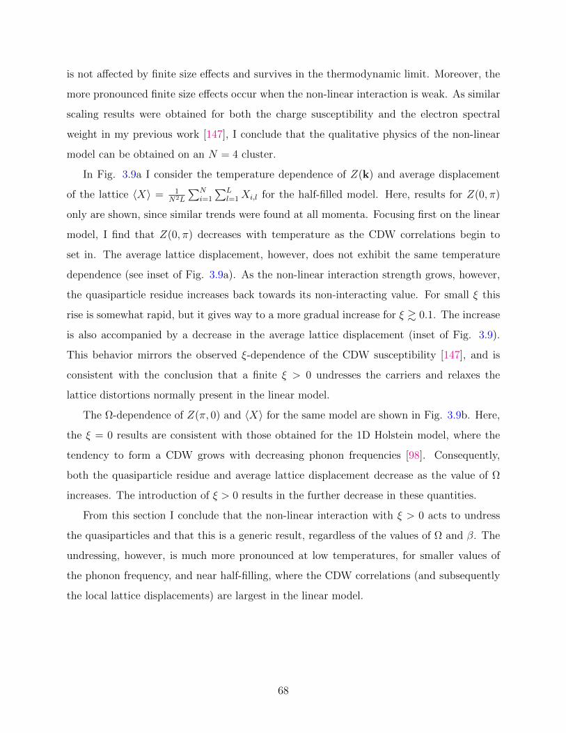
is not affected by finite size effects and survives in the thermodynamic limit. Moreover, the

more pronounced finite size effects occur when the non-linear interaction is weak. As similar

scaling results were obtained for both the charge susceptibility and the electron spectral

weight in my previous work [147], I conclude that the qualitative physics of the non-linear

model can be obtained on an N = 4 cluster.

In Fig. 3.9a I consider the temperature dependence of Z(k) and average displacement

of the lattice 〈X〉 = 1N2L

∑Ni=1

∑Ll=1Xi,l for the half-filled model. Here, results for Z(0, π)

only are shown, since similar trends were found at all momenta. Focusing first on the linear

model, I find that Z(0, π) decreases with temperature as the CDW correlations begin to

set in. The average lattice displacement, however, does not exhibit the same temperature

dependence (see inset of Fig. 3.9a). As the non-linear interaction strength grows, however,

the quasiparticle residue increases back towards its non-interacting value. For small ξ this

rise is somewhat rapid, but it gives way to a more gradual increase for ξ & 0.1. The increase

is also accompanied by a decrease in the average lattice displacement (inset of Fig. 3.9).

This behavior mirrors the observed ξ-dependence of the CDW susceptibility [147], and is

consistent with the conclusion that a finite ξ > 0 undresses the carriers and relaxes the

lattice distortions normally present in the linear model.

The Ω-dependence of Z(π, 0) and 〈X〉 for the same model are shown in Fig. 3.9b. Here,

the ξ = 0 results are consistent with those obtained for the 1D Holstein model, where the

tendency to form a CDW grows with decreasing phonon frequencies [98]. Consequently,

both the quasiparticle residue and average lattice displacement decrease as the value of Ω

increases. The introduction of ξ > 0 results in the further decrease in these quantities.

From this section I conclude that the non-linear interaction with ξ > 0 acts to undress

the quasiparticles and that this is a generic result, regardless of the values of Ω and β. The

undressing, however, is much more pronounced at low temperatures, for smaller values of

the phonon frequency, and near half-filling, where the CDW correlations (and subsequently

the local lattice displacements) are largest in the linear model.

68

Figure 3.9: The (a) temperature and (b) Ω dependence of the quasiparticle residue inthe half-filled model as a function of non-linear coupling strength ξ. The insets show thecorresponding expectation value of the lattice displacement. All results are obtained on anN = 4 cluster and with a linear coupling λ = 0.25. Error bars smaller than the marker sizehave been suppressed for clarity.

69

3.2.3 Electron and Phonon energetics

The average kinetic energy of the electronic subsystem 〈KE〉el = −t∑〈i,j〉,σ〈c

†i,σcj,σ〉 at β =

4/t is shown in Fig. 3.10. Results are shown as a function of band filling 〈n〉 for various

ξ and for a linear coupling λ = 0.25. For ξ = 0 the total kinetic energy −〈KE〉e increases

as a function of 〈n〉 as higher momentum states are populated in the Fermi sea, however,

the total kinetic energy saturates as the filling increases beyond 〈n〉 > 0.6. This is due to

the saddle point in the band dispersion at (0, π) and is also present in the non-interacting

model (indicated by the dashed line). When the non-linear interaction is added I see an

overall increase in the total kinetic energy, which tends towards the non-interacting value

at all fillings for large ξ. This again reflects the undressing of the quasiparticles and the

subsequent increase in mobility of the electronic subsystem.

Fig. 3.10b shows the corresponding e-ph interaction energy, defined as 〈E〉e−ph =∑i〈g1niXi + g2niX

2i 〉. Unsurprisingly, the total e-ph interaction energy increases with band

filling as both the average number of electrons per site and the average lattice displacement

increase. This is most evident in the linear model (ξ = 0). Increasing the value of ξ naturally

leads to smaller lattice displacements and a significant decrease in 〈E〉e−ph.

The average kinetic 〈KE〉ph and potential 〈PE〉ph energies of the lattice are shown in Figs.

3.11a and 3.11b, respectively. They are given by

〈KE〉ph =1

2∆τ− M

2

⟨∑i,l

(Xi,l+1 −Xi,l

∆τ

)2 ⟩(3.10)

〈PE〉ph =MΩ2

2

⟨∑i,l

X2i,l

⟩. (3.11)

(The factor of 12∆τ

appearing in Eq. (10) is a Euclidean correction introduced by the Wick

rotation to the imaginary-time axis [113].)

In the linear model I see a very weak variation in the phonon kinetic energy as a function

of filling, with a slight decrease observed near half-filling when the CDW correlations increase.

This is consistent with prior observations of the lattice kinetic energy in the vicinity of a

CDW transition in the Hubbard- Holstein model [113]. The average potential energy of the

lattice grows as the average number of carriers per site increases. When the non-linearity

70

-2

-1

0

<KE>

el [t

]<E

> e-ph

[t]

(c) N = 8, β = 5/t

= 0.00= 0.05= 0.10= 0.30

0

1

2

0 0.2 0.4 0.6 0.8 0 0.2 0.4 0.6 0.8 1<n>

(b)

(a) N = 4, β = 4/t

(d)

ξ = 0.00ξ = 0.05ξ = 0.10ξ = 0.25

Figure 3.10: (color online) (a) The electron kinetic energy 〈KE〉el and (b) the e-ph energy〈E〉e−ph as a function of band filling 〈n〉 for various non-linear interaction strengths ξ, asindicated. Results are obtained on an N = 4 cluster and with a linear coupling λ = 0.25,phonon frequency Ω = t, and an inverse temperature β = 4/t. The dashed lines in panels(a) and (c) indicate the non-interacting result. (c) and (d) show corresponding results for alarger N = 8 cluster and β = 5/t. The remaining parameters are the same as in (a) and (b).Error bars smaller than the marker size have been suppressed for clarity.

71

0.24

0.32

0

1

0 0.2 0.4 0.6 0.8 1

<PE>

ph [t

]<K

E>ph

[t]

0 0.2 0.4 0.6 0.8<n>

0

(b)

(a) N = 4, β = 4/t

(d)ξ = 0.00ξ = 0.05ξ = 0.10ξ = 0.30

ξ = 0.00ξ = 0.05ξ = 0.10ξ = 0.25

(c) N = 4, β = 5/t

Figure 3.11: (color online) The phonon (a) kinetic energy 〈KE〉ph and (b) potential energy〈PE〉ph as a function of band filling 〈n〉 for various of the non-linear interaction strengthξ, as indicated in panel (b). Results are obtained on an N = 4 cluster and with a linearcoupling λ = 0.25, Ω = 1,and β = 4/t. (c) and (d) show similar results obtained on a largerN = 8 cluster with β = 5/t. Error bars smaller than the marker size have been suppressedfor clarity.

72

is introduced and the lattice distortions diminish (see 3.9b, inset), and I see an increase in

the lattice kinetic energy, which is attributed to the hardening of the phonon dispersion. At

the same time, I see a decrease in the total lattice potential energy. Here, the non-linear

interaction has two opposing effects: the increase in the phonon frequency increases the

lattice potential energy while the decrease in the effective linear coupling decrease the net

lattice distortions and subsequently lowers the potential energy. My results indicate that

the latter effect has the stronger impact.

The energetics reported here are completely consistent with the conclusion that the

non-linear interaction acts to harden the phonon frequency and weaken the effective linear

interaction, which results in an undressing of the quasiparticles for ξ > 0.

3.2.4 Phonon Spectral Properties

In the linear Holstein model the formation of the CDW phase is accompanied by a softening of

the phonon dispersion to zero energy at the nesting wavevector Q = 2kF = (π, π) [195, 172,

252, 262]. This softening is generated by the strong nesting condition of the non-interacting

Fermi surface. The inclusion of the non-linear e-ph interaction is therefore expected to

modify the phonon dispersion in two important ways: first, it will undo the softening at Q

as the CDW correlations are suppressed. Second, it will result in an overall renormalization

of the phonon frequency, as showed in the Ref. [1]. I confirm these expectations in this

section by examining the phonon spectral function B(q, ν) and the phonon density of states

(DOS) Nph(ν) = 1N2

∑qB(q, ν).

In the non-interacting limit, B(q, ν) and Nph(ν) are delta functions centered at the bare

phonon frequency Ω. In the presence of a non-zero linear interaction only, this distribution

shifts to lower energy and broadens. This is illustrated in Figs. 3.12 and 3.13a, which plot

Nph(ν) and the momentum-resolved phonon spectral function B(q, ν), respectively, for the

half-filled model. These results were obtained on N = 8 clusters, with a linear coupling

λ = 0.25, Ω = t, and at an inverse temperature of β = 4/t. Due to the finite value of λ,

the phonon frequency softens from its non-interacting value and Nph(ν) for the linear model

consists of a broad, asymmetric distribution centered at ∼ 0.60t. The asymmetry in Nph(ν)

reflects the momentum dependence of the softening and the low-energy spectral weight in

73

0 0.5 1 1.5 2 2.5

0

0.5

1

ν [t]

ξ = 0.00 ξ = 0.02 ξ = 0.05 ξ = 0.25 ξ = 0.50

Nph

(ν)

N = 8, Ω = t , λ = 0.25β = 4/t, Δτ = 0.1/t

Figure 3.12: (color online) The phonon density of states Nph(ν) = 1N

∑qB(q, ν) for

the half-filled model as a function of the non-linear interaction strength. The remainingcalculation parameters are as indicated.

74

Figure 3.13: (color online) The momentum resolved phonon spectral function B(q, ν) forthe half-filled model and for various values of the non-linear interaction strength, as indicatedin each panel. Results were obtained on an N = 8 cluster with λ = 0.25, Ω = t, β = 4/tand ∆τ = 0.1/t. The black squares indicate the position of the peak in the phonon spectralfunction.

75

B(Q, ν), coupled with the requirement that B(0) = 0 for bosons. This is more easily seen

in the momentum-resolved spectral function (Fig. 3.13a), which has a clear Kohn anomaly

at Q = (π, π).

Two prominent changes occur when ξ 6= 0. First, the peak in the DOS shifts to higher

energies, which verifies the hardening of the effective phonon frequency. This behavior is

also clearly seen in the momentum resolved spectral functions, shown in Fig. 3.13. Second,

the pronounced Kohn anomaly begins to disappear as the CDW correlations are suppressed

with increasing values of ξ. Both of these results confirm my expectations.

3.2.5 Mean-field Treatment of the quadratic e-ph interaction

As I have repeatedly seen, the non-linear e-ph interaction acts to renormalize both the bare

linear interaction strength λ and the bare phonon frequency Ω. Both of these effects can

be qualitatively understood at the mean-field (MF) level for the quadratic model, where an

effective linear Hamiltonian is obtained by performing a MF decoupling of the interaction

terms proportional to b†ib†i and bibi [1]. The resulting effective MF Hamiltonian is

HMF = Hel +∑i

ΩMF

(b†ibi +

1

2

)+∑i,σ

gMF ni,σ

(b†i + bi

),

where ΩMF = Ω+2g2 and gMF = g1(1− 2g2

Ω+4g2) are the renormalized phonon frequency and e-

ph coupling constants, respectively. One immediately sees that the quadratic e-ph interaction

leads to a softening (hardening) of the phonon frequency and an increase (decrease) in the

effective linear interaction strength g1 for ξ < 0 (ξ > 0). These two effects combine to

produce an overall increase (decrease) in the strength of the effective dimensionless coupling

λeff ∝g2MF

ΩMF.

The MF treatment of the non-linear interaction is consistent with the general trends

reported here and in Refs. [147] and [1]. I stress, however, that the MF description only

provides a qualitative picture of the non-linear effects. To illustrate this, I compare my

DQMC results for the full non-linear Hamiltonian against the predictions obtained from two

sets of effective linear models. The first is the MF-derived model defined by Eq. (3.12). The

76

second is the set of effective linear models whose parameters are obtained by tuning the Ωeff

and geff to reproduce the electronic properties of the system.

I consider the MF-derived model first. Fig. 3.14 compares the results for the quasiparticle

residue, χC(π, π), and the pair-field susceptibility χSC calculated using the full non-linear

model [Eq. (3.2)] to results obtained from a DQMC simulation of the corresponding MF-

derived linear model [Eq. (3.12)] at half-filling. I find that the MF model does a poor job in

quantitatively capturing the electronic properties; it underestimates both the quasiparticle

residue Z(0, π) and the tendency towards the formation of a CDW when compared to the full

non-linear model. The MF model also over-predicts the magnitude of the superconducting

pair-field susceptibility when ξ is large and under-predicts it when ξ is small.

The results shown in Fig. 3.14 demonstrate that the MF treatment of the quadratic

interaction can only provide a qualitative picture of the physics of the non-linear model;

however, another choice in effective model might do a better job. I explored this possibility

by adjusting the effective coupling strength in the linear model such that the linear model

reproduced the electronic properties of the full non-linear model. This procedure was

performed for two choices in the phonon frequency. First, I set the phonon frequency equal to

the bare value and adjusted the value of the coupling strength to reproduce the quasiparticle

residue, as shown Fig. 3.15a. The value of the linear coupling strength geff needed to

produce this agreement is shown in the inset (black solid 4), where it is compared against

the corresponding value of gMF = g1+2g2. By tuning the value of geff I am able to accurately

capture the quasiparticle residue. The charge and superconducting pair-field susceptibilities

are also well reproduced, indicating that this effective model is capable of capturing the

electronic properties of the system. But when I examine the phonon properties (Figs. 3.15c

& 3.15d) I find some disagreement, particularity with respect to the predicted kinetic energy

of the lattice, where the linear model systematically under-predicts the correct results.

The comparison between the two models can be improved somewhat if I set the phonon

frequency to be equal to ΩMF and again readjust the value of geff . This case is shown in Fig.

3.15e-h. Using this choice I am again able to accurately capture the electronic properties

and improve the comparison between the kinetic energy. But this comes at the expense of

the level of agreement between the average lattice potential energy and the average lattice

77

Figure 3.14: (color online) A comparison of (a) the quasiparticle residue and (b) CDWχC(π, π) and pair field susceptibilities χSC obtained from the non-linear model and itseffective linear model, as defined in the main text. The bare linear coupling and phononfrequency are λ = 0.25 and Ω = t, respectively. In both cases results are obtained on anN = 8 cluster and at an inverse temperature of β = 4/t. Error bars smaller than the markersize have been suppressed for clarity.

78

0.6

0.8

1

ξ ξ

(a) (e)

0

0.4

0.8(b)

non-linear modeleff. model, Ω = teff. model, Ω = ΩMF

(f)

0

0.2

0.4

(c) (g)

0.4

0.8

1.2

0 0.1 0.2 0.3 0.4(d)

0 0.1 0.2 0.3 0.4 0.5(h)

0.5

1

g eff

g eff

ξ

0.5

1

ξ

<X>

[a]

<PE>

ph/3

, <K

E>ph

[t]

χ c(π, π

)/10,

χsc

Z(

0, π

)

0 0.2 0.4 0 0.2 0.4

Figure 3.15: (color online) A comparison of the results obtained for the full non-linearmodel and an effective linear model where the value of the e-ph coupling constant has beenadjusted to reproduce the electronic properties of the non-linear model. Panels (a)-(d) showa comparison for an effective linear model with Ω = t, equal to the bare phonon frequency.Panels (e)-(f) show a comparison for an effective linear model with Ω = ΩMF . The toprow [panels (a) & (e)] compares the quasiparticle residues obtained with both models. Thesecond row [panels (b) & (f)] shows the resulting charge (solid lines) and pair-field (dashedlines) susceptibilities. The third row [panels (c) & (g)] show the resulting phonon potentialand kinetic energies. The potential energy has been divided by a factor of three and isindicated by the solid lines while the kinetic energy is indicated by the dashed lines. Finally,the bottom row [panels (d) & (h)] show the average value of the lattice displacement. Theremaining parameters of the simulation are β = 4/t and N = 8.

79

displacement. From this I conclude that an effective linear model cannot capture both the

electronic and phononic properties of the non-linear model, for a fixed value of the phonon

frequency. These results show that while the qualitative effects can be understood using

an effective linear model, the full non-linear interaction should be retained if one wishes

to accurately capture the effects of the non-linear interaction on both the phononic and

electronic properties of the system. A similar conclusion was reached in Ref. [1] in the single

carrier limit.

3.2.6 Negative values of ξ

I have shown that a positive (ξ > 0) non-linear coupling results in a hardening of the phonon

frequency and a renormalization of the effective linear e-ph coupling to weaker values. But

what about the case when ξ < 0, where the MF model predicts an enhanced effective linear

coupling? Before examining this case, one should note that a large negative ξ necessarily

requires the inclusion of additional anharmonic terms in the lattice potential [2]. For ξ < 0

(g2 < 0) the phonon frequency given by Ωeff = Ω + 2g2 can become negative for sufficiently

large values of g2, indicating an instability in the lattice. In this event the anharmonic

terms of the lattice potential are required to maintain stability. At present, my codes do not

contain such terms and I am unable to examine this case in great detail. I therefore restrict

ourselves to a larger value of Ω = 2t and small values of |g2| in order to get a feel for the

g2 < 0 regime while ensuring the stability of the lattice.

Fig. 3.16a shows the quasiparticle residue, χC(π, π), and χSC as a function of band filling

for various values of ξ < 0. These results were obtained for a linear coupling of λ = 0.25

and on an N = 8 cluster. I find that the quasiparticles are more effectively dressed when

ξ < 0, and the quasiparticle residue is much smaller for all fillings when increasing negative

quadratic interactions are included. The CDW correlations are also significantly enhanced,

as reflected in the charge susceptibility shown in Fig. 3.16b. Both of these observations are

in line with the expected increase in the effective linear coupling. Furthermore, since the

CDW phase directly competes with s-wave superconductivity, the pair-field susceptibility

is suppressed at filling values where the CDW correlations dominate. In addition, I also

see a noticeable decrease in the pair-field susceptibility at band fillings where the CDW

80

Figure 3.16: (color online) (a) the quasiparticle residue and (b) CDW χC(π, π) (opensymbols) and pair field susceptibilities χSC (solid symbols) as a function of band filling. Theparameters are set as: λ = 0.25, Ω = 2t, β = 4. The results are obtained on an N = 8cluster. Error bars smaller than the marker size have been suppressed for clarity.

81

does not dominate. This suggests that the negative non-linear interaction has a detrimental

effect on the superconducting transition temperature, which stems from the decrease in the

quasiparticle residue. Fig. 3.17 plots the momentum dependence of the charge susceptibility

χ(q) as a function of negative ξ at half filling, where it is clear that the dominant CDW

correlations are still being set by the Fermi surface nesting condition.

3.3 Conclusion

We have examined a non-linear Holstein model on a two-dimensional square lattice and at

finite temperatures and carrier concentrations using determinant quantum Monte Carlo. The

competition between CDW and superconducting correlations was re-examined as a function

of the non-linear e-ph interaction strength. The primary effect of the positive non-linear

e-ph interaction is a dramatic suppression of the CDW correlations that dominate the linear

model. A less pronounced effect was observed for the superconducting correlations. These

effects are attributed to a combined hardening of the phonon mode and renormalization

of the effective linear coupling by the non-linear terms. The net result is an overall

reduction in the e-ph interaction strength. This assumption is corroborated by checking

quasiparticle properties. It found that a positive nonlinear interaction term serves to

undress the quasiparticles leading to carriers with lighter effective masses. This leads to

changes in the energetics of both the electrons and phonons, as well as the relaxation of

the local lattice distortions surrounding each carrier. I have also examined the case when

the quadratic e-ph interaction has the opposite sign as the linear interaction, although this

case cannot be explored in detail without the inclusion of additional anharmonic terms in

the lattice potential. Nevertheless, in my limited range of accessible parameters, I found

that a quadratic interaction results in an increased dressing of the carriers and an enhanced

tendency towards the formation of a Q = (π, π) CDW ordered phase.

While many of the effects we have discussed can be understood qualitatively at the mean-

field level, we have demonstrated that the quantitative effects can only be captured by the

full non-linear model. Specifically, the effective linear models fail to simultaneously capture

the electronic and phononic properties. Therefore the full non-linear model must be retained

82

0

20

40

60

80

(0,0) ( ,0) ( , ) (0,0)

C(q

)

Momentum [1/a]

N = 8, = 0.25, = 2t, = 4,

Δτ = 0.1/t, <n> = 1

= 0.00 =-0.02 =-0.05

Figure 3.17: (color online) The momentum dependence of the charge susceptibility χ(q)as a function of non-linear interaction strength ξ < 0 at half filling. The parameters are setas: λ = 0.25, Ω = 2t, β = 4. The results are obtained on an N = 8 cluster. Error barssmaller than the marker size have been suppressed for clarity.

83

if one wishes to accurately capture the properties of the electrons and the phonons. Our

results are in good agreement with the results obtained in the single particle limit,[1] and

show that non-linearities are relevant at finite carrier concentrations.

My results also have implications for pump-probe experiments aimed at studying the

strength of the e-ph interaction. For example, the higher-order interaction terms can become

important in such experiments if the external field drives the lattice to large displacements,

even if the electron-lattice coupling at equilibrium is weak. Therefore, if the lattice is pumped

too strongly, there is a danger that the non-linearity will enter and renormalize the effective

coupling to smaller values. In doing so, one could drive the system hard enough that they

extinguish the interactions they are trying to probe. Obviously, this will be less of an issue

if the pump pulses are weak and the lattice is only slightly perturbed; however, these effects

may become extremely important if the lattice is strongly pumped as our results show that

even a small non-linear contribution can have an order-of-magnitude impact. Moving forward

it will be important to study the role of non-linear electron-lattice coupling and anharmonic

lattice potentials as the community continues to study systems driven far from equilibrium.

Finally, these results call for a re-evaluation of claims of high-Tc superconductivity

mediated by non-linear e-ph coupling [192]. I stress, however, that physics arising from

the non-linear coupling is different from anharmonic effects due to the lattice potential,

which are thought to play key role in MgB2 [277] and KOs2O6 [39].

84

Chapter 4

The orbital-selective Mott phase

In this chapter, I study non-local correlations in a three-orbital Hubbard model defined on

an extended one-dimensional chain using determinant quantum Monte Carlo. Besides, some

DMRG calculations have been done to support my DQMC results by Nitin Kaushal. I focus

on a parameter regime with robust Hund’s coupling, which produces an orbital-selective

Mott phase (OSMP) at intermediate values of the Hubbard U . The OSMP has been widely

studied using dynamical mean field theory, which neglects non-local correlations. In this

chapter, I will show the momentum dependence of the OSMP and discuss the importance of

the non-local correlations. The results presented in this chapter have appeared in Ref. [148].

In recent years the scientific community renewed its interest in understanding the

properties of multi-orbital Hubbard models, and this has been intensified by the discovery

of the iron-based superconductors [111, 240, 57, 220]. On a theoretical front, this is

a challenging problem due to a lack of non-perturbative methods for treating multi-

orbital Hubbard models at intermediate or strong couplings and on extended systems.

Nevertheless, considerable progress has been made using mean-field-based approaches

[220, 282, 71, 79, 291, 126, 266, 154, 180, 178, 187, 233, 72, 153], resulting in new concepts

such as that of a Hund’s metal [291, 278, 79, 133] and the orbital-selective Mott phase

(OSMP) [5, 79]. These concepts are central to understanding the paradoxical appearance

of both localized and itinerant characteristics in many multi-orbital systems [179, 169] and

bad metallic behavior in the presence of sizable electronic correlations [179].

85

The most widely used numerical approach in this context is single-site multi-orbital

dynamical mean-field theory (DMFT) [78, 220]. Generally speaking, DMFT maps the

full lattice problem onto an impurity problem embedded in an effective medium, which

approximates the electron dynamics on a larger length scale as a local renormalization [78].

While this technique has had considerable success in addressing many aspects of the OSMP

and other physics related to the multi-orbital problem [126, 154, 38, 153, 21, 180, 178, 266,

106, 82], it is unable to capture spatial fluctuations and non-local correlations encoded in the

k-dependent self-energy Σ(k, ω). This is a potential short coming as non-local correlations

are known to have an impact in the case of the single-band Hubbard model [85, 199]. It

is therefore important to assess the importance of such non-local effects on multi-orbital

properties such as the OSMP.

To date, most non-perturbative studies of non-local effects have used cluster DMFT or

the dynamical cluster approximation (DCA) [194, 139, 140, 16, 144, 233]; however, these

techniques are typically limited to a handful of sites when multiple orbitals are included in

the basis. This is due to technical issues related to each choice in impurity solver, such as

the Fermion sign problem in the case of quantum Monte Carlo or the exponential growth

of the Hilbert space in the case of exact diagonalization. As a result, these studies have

only addressed short-range spatial fluctuations. One study of the OSMP has been carried

out on a larger two-dimensional cluster using determinant quantum Monte Carlo (DQMC).

In that case, however, the OSMP was imposed by the model by assuming that electrons

in a subset of orbitals were localized as Ising spins [29]. In light of these limitations it is

desirable to find situations where multi-orbital physics can be modeled on extended clusters

that support long-range spatial fluctuations and where the properties under study emerge

from the underlying many-body physics of the model.

In this regard, one dimensional (1D) models are quite promising. For example, two

recent density matrix renormalization group (DMRG) studies have been carried out for an

effective 1D three-orbital model representative of the iron-based superconductors [218, 219].

More recently, it was demonstrated that DQMC simulations for a simplified version of the

same model can also be carried out to low temperatures due to a surprisingly mild Fermion

sign problem [156]. These observations open the doorway to non-perturbative studies of this

86

model on extended clusters, thus granting access to the momentum-resolved self-energies and

non-local correlations. 1D studies along these lines are also directly relevant for the recently-

discovered quasi-1D selenide Ba1−xKxFe2Se3 [35, 34, 203, 63, 160, 159]. In this context, it is

important to note that DMFT becomes more accurate in higher dimensions and therefore

one expects its ability to describe multi-orbital Mott physics in 1D to be diminished.

Motivated by these considerations, I examine the properties of a three-orbital Hubbard

Hamiltonian on an extended 1D cluster using DQMC and DMRG, with a particular focus

on its k-resolved self-energies and spectral properties. I thus gain explicit access to non-

local correlations occurring on longer length scales than those addressed in previous non-

perturbative studies. In general, I find that the OSMP leads to a mixture of localized and

itinerant bands, where the former are characterized by a localized (momentum-independent)

self-energy while the latter exhibits significant non-local (momentum-dependent) correla-

tions. This also leads to a band-dependent relative shift of the underlying electron- and

hole-like bands. I also identify an insulating state driven by orbital ordering in a region of

parameter space previously associated with an OSMP [218, 219].

Before proceeding, I clarify my definition for the OSMP region and its critical

temperature. This region is defined here by the situation where the population of a particular

orbital (orbital three) converges to 〈n3〉 = 1 while a gap simultaneously opens in the density

of states for this orbital. While this is a sound operative definition of my purpose, there

are subtleties that must be addressed as a warning to the reader. In the context of DMFT,

investigations of multiorbital models [199, 153] in the plane defined by temperature T and

coupling strength U/W (W is the bandwidth) show that there is an analytic connection

between the Mott insulating side of a line of first order transitions and the weak coupling

metallic side. The line of first-order transitions survives the introduction of temperature,

but it has an end point at a finite T in analogy to the gas/liquid transition. For example,

in the analysis of the localized orbital reported in Ref. [153], the quasiparticle weight Z is

claimed to be nonzero at finite T on the insulating side (although it is extremely small at

low temperatures). I believe that Z being zero or very small is similar to the condition that

my localized orbital’s population is equal to or very close to one. As a consequence, what

I have defined as a transition towards an OSMP may in fact be a region where 〈n3〉 ≈ 1

87

but not exactly 1. If this is the case, then my critical temperature is in reality a very sharp

crossover towards a region that only reaches true OSMP characteristics at T = 0 (or at the

much lower temperature where magnetic block correlations develop). Note that DMFT is

valid in infinite dimension, while my problem is in the opposite limit, so these arguments

are all qualitative at best. In spite of these subtleties, I will refer to the region below my

critical temperature defined by 〈n3〉 converging to 1 as an OSMP for simplicity, with the

caveat that exact OSMP characteristics may be reachable only at lower T .

4.1 One-dimensional three-orbital Hubbard model

I study a simplified three-orbital model defined on a 1D chain as introduced in Ref.

[218]. This model displays a rich variety of phases including block ferromagnetism,

antiferromagnetism, Mott insulting phases, metallic and band insulating phases, and several

distinct OSMPs [218, 219, 156]. The Hamiltonian is H = H0 +Hint, where

H0 = −∑〈i,j〉σ,γ,γ′

tγγ′c†i,γ,σcj,γ′,σ +

∑i,σ,γ

(∆γ − µ)ni,γ,σ (4.1)

contains the non-interacting terms of H, and

Hint = U∑i,γ

ni,γ,↑ni,γ,↓ +

(U ′ − J

2

)∑i,σ,σ′

γ<γ′

ni,γ,σni,γ,σ′

+J∑i,γ<γ′

Szi,γS

zi,γ′ (4.2)

contains the on-site Hubbard and Hund’s interaction terms. Here, 〈. . . 〉 denotes a sum over

nearest-neighbors, c†i,γ,σ (ci,γ,σ) creates (annihilates) a spin σ electron in orbital γ = 1, 2, 3

on site i, ∆γ are the on-site energies for each orbital, Szi,γ is the z-component of the spin

operator Si,γ, and ni,γ,σ = c†i,γ,σci,γ,σ is the particle number operator.

Note that in Eq. (4.2) I have neglected the pair-hopping and spin-flip terms of the

interaction. These terms can have an important influence on the details of the OSMP in

higher dimensions. In the context of the current model, however, a previous DMRG [156]

88

study found that these terms only alter the location of the phase boundaries and do not

qualitatively change the nature of the underlying phases. Since my focus here is on the

non-local correlations associated with these phases, rather than subtle issues regarding their

boundaries, I neglect the spin-flip and pair hopping terms in order to manage the Fermion

sign problem in the DQMC calculations.

Following Ref. [218], I set t11 = t22 = −0.5, t33 = −0.15, t13 = t23 = 0.1, t12 = 0,

∆1 = −0.1, ∆2 = 0, and ∆3 = 0.8 in units of eV while the chemical potential µ is adjusted

to obtain the desired filling. These parameters produce a non-interacting band structure

analogous to the iron-based superconductors, with two hole-like bands centered at k = 0

and an electron-like band centered at k = π/a, where a is the lattice constant, as shown in

Fig. 4.1. Due to the weak inter-orbital hopping, each of the bands is primarily derived from

a single orbital, as indicated by the line thickness and colors in Fig. 4.1. One can therefore

(loosely) regard the orbital character as an indicator of the band in this model. For example,

the top most band is primarily composed of orbital γ = 3. The total bandwidth of the non-

interacting model is W = 4.9|t11| = 2.45 eV. This will serve as the unit of energy. I further set

a = 1 as the unit of length. The interaction parameters are fixed to U ′ = U − 2J , J = U/4,

while U is varied. This parameter regime results in a robust OSMP for intermediate values

of U [156, 219, 218], which is my focus here.

The model is studied using non-perturbative DQMC method. The primary drawback to

DQMC is the Fermion sign problem [157, 105], which typically limits the range of accessible

temperatures for many models. Indeed, when the spin-flip and pair hopping terms of the

Hund’s interaction are included in the Hamiltonian, I find that the model has a prohibitive

sign problem. But when these terms are neglected the corresponding sign problem becomes

very mild [156], even in comparison to similar simplified multi-orbital models in 2D [212, 28].

Given that these terms do not qualitatively affect the phase diagram [156] for current model,

I have neglected them here. Unless otherwise stated, all of my DQMC results were obtained

on an L = 24 site cluster with periodic boundary conditions and for an average filling of

〈n〉 = 4 electrons, which corresponds to 2/3 filling.

89

−1 −0.5 0 0.5 1−0.8

−0.6

−0.4

−0.2

0

0.2

Momentum (π/a)

Ener

gy (W

)γ = 1γ = 2γ = 3

Figure 4.1: (color online) A fat band plot of the non-interacting band structure at a totalfilling of 〈n〉 = 4, where the thickness of the lines indicates the majority orbital content ofthe band. The top most band has the narrowest bandwidth and is primarily of orbital 3character. The lower two bands disperse over a much larger energy range and are primarilycomposed of orbitals 1 and 2, respectively.

90

4.2 Results

4.2.1 Low temperature properties

I first focus on the low temperature β = 73.5/W , where I can identify the ground state

properties. Here, I set the chain length L = 16. Fig. 4.2a plots the average sign value as a

function of U . The average value of the sign is quite high for most values of U , indicating

the low-temperature properties can be accessed. It is interesting to observe that the sign

problem is at its worst when U/W ∼ 0.4, which is near the phase boundary between the

metallic and orbital-selective Mott phases for this model. This phase transition between the

metallic and OSMP can be easily identified in Fig. 4.2b, which plots the U dependence of

orbital occupations. As increasing U , n3 increases and finally is locked at 1, which implying

that a Mott gap is opened on the orbital 3. While, n1 and n2 are still fractional in that orbital

1 and orbital 2 are metallic phases. The OSMP sits in U/W ∈ [0.4, 1]. Fig. 4.2 c shows

the magnetic structure factor on the orbital 3 at U/W = 0.01 and U/W = 0.8, respectively.

The magnetic structure factor is defined as Sf (q) = 1/L∑

j,m eiq(rj−rm)Sj,γ=3 · Sm,γ=3. In

the metallic phase (U/W = 0.01), the orbital 3 is paramagnetic, while in the OSMP, the

magnetic structure on the orbital 3 has a peak around q = 0.5π/a, implying the magnetic

structure on the chain is the block spin state [156, 219, 218]. As increasing the temperature

to β = 19.6/W , the block spin state disappears (see Fig. 4.2d) and the magnetic structure

on the orbital 3 becomes disordered. In the following, I will show the Mott gap is still there

at this elevated temperature. This result shows that the insulating state on the orbital 3 is

a Mott insulator rather than slater insulator.

4.2.2 Self-energies in the OSMP

I then study some of the standard metrics for the formation of an OSMP as a function of

temperature, namely the average filling per orbital and the quasiparticle residue Zγ(k, iωn).

DQMC results for 〈n〉 = 4 and U/W = 0.8 are summarized in Fig. 4.3. The temperature

dependence of the individual orbital occupations 〈nγ〉, plotted in Fig. 4.3a, has the standard

indications of the formation of an OSMP: At high temperature (small β) I see noninteger

fillings for all three orbitals. As the temperature is lowered (large β), however, orbitals one

91

0

0.2

0.4

0.6

0.8

1

0.01 0.1 1

<si

gn

>

U/W

(a)

β = 73.5/W

0.6

0.8

1

1.2

1.4

1.6

1.8

0.01 0.1 1

<n

>

U/W

β = 73.5/W N = 16

n = 4

(b)

M OSMP

n1n2n3

0

0.4

0.8

1.2

0 0.25 0.5 0.75 1

Sf(

q)

q (π/a)

(c)

β = 73.5/W

U/W = 0.01

U/W = 0.8

0

0.4

0.8

1.2

0 0.25 0.5 0.75 1

Sf(

q)

q (π/a)

(d)

β = 19.6/W

L = 24

Figure 4.2: (color online) (a) the average sign value as a function of the Hubbard U . (b)The U dependence of orbital occupations. (c) The magnetic structure factor of the orbital3 at U/W = 0.8. In (a)-(c), the temperature is β = 73.5/W . (d) The magnetic structurefactor of the orbital 3 at U/W = 0.8 and β = 19.6/W . In each panel, error bars smallerthan the marker size have been suppressed for clarity.

92

Figure 4.3: (color online) Orbitally resolved electronic properties for U/W = 0.8 (W =2.45 eV) at different temperatures. (a) The temperature dependence of orbital occupations.(b) The orbital resolved quasiparticle residue Zγ(k, iπ/β) at an inverse temperature β =19.6/W . (c) The normalized electron self energies ImΣγ(k, iπ/β) at ωn = π/β as a functionof momentum. Each curve is normalized by its k = 0 value to highlight the overall momentumdependence. The scale is determined by ImΣγ(0, iπ/β) = −0.53, −0.57, and −2.53 for γ =1, 2, 3, respectively, and in units of the bandwidth W . The blue, red, and green dash lines in(b) and (c) correspond to the bare Fermi momentum of the non-interacting bands. Panel (d)shows orbitally resolved quasiparticle residues Zγ(k

0F, iπ/β) and self energies ImΣγ(k

0F, iπ/β)

at Fermi momentum as a function of temperature. In each panel, error bars smaller thanthe marker size have been suppressed for clarity.

93

and two smoothly approach fillings of ∼ 1.53 and ∼ 1.47, respectively, while orbital three

locks into an integer value of exactly 1. In many studies the “stiffness” of orbital three’s

integer occupation is taken as an indication of an OSMP [218, 219], where this orbital has

undergone a transition to a Mott insulating state while remaining orbitals host itinerant

electrons. Indeed, for U/W = 0.8 and at low temperature, the integer filling observed in

orbital three is robust against changes in the chemical potential and interaction strength

U (see Refs. [156, 218, 219]). This indicates that this integer filling is indeed driven by

the interaction and is not a simple coincidence of the non-interacting band parameters.

However, as I will show, this does not always correspond to an OSMP. For U/W = 0.8

the two fractionally filled orbitals are in fact itinerant, but for larger values of U/W these

same orbitals retain a fractional filling but are driven into an insulating state by the onset

of orbital ordering in these two orbitals.

The mixed itinerant/localized nature of the OSMP at U/W = 0.8 is reflected in the

momentum dependence of quasi-particle residue Zγ(k, iπ/β) and the orbitally resolved

normalized self-energies R(k) = ImΣγ(k, iπ/β)/ImΣγ(0, iπ/β), plotted in Figs. 4.3c and

4.3d, respectively, for ωn = π/β. The self-energy is extracted from the dressed Green’s

function using Dyson’s equation

G−1(k, iωn) = G−10 (k, iωn)− Σ(k, iωn), (4.3)

where the G notation denotes a matrix in orbital space, G0(k, iωn) = [iωnI − H0(k)]−1 is the

non-interacting Green’s function, and H0(k) is the Fourier transform of the non-interacting

Hamiltonian defined in orbital space. The quasi-particle residue is obtained from the diagonal

part of the self-energy using the identity

Z(k, iπ/β) =

(I − ImΣ(k, iπ/β)

π/β

)−1

, (4.4)

where I is a 3× 3 unit matrix.

As can be seen from Fig. 4.3c, the self-energies for each orbital have a sizable k-

dependence at this temperature. (In this case I have normalized the self-energy by its

94

value at k = 0 in order to highlight the overall momentum dependence. The magnitude

of ImΣγ(0, iπ/β) is given in the figure caption.) In the case of orbitals one and two, the

magnitude of the self-energy varies by nearly 50% throughout the Brillouin zone. In contrast,

the momentum dependence of Σ3(k, iπ/β) for orbital three is much weaker, varying by only

5-10% and reflecting the localized nature of the carriers in these orbitals. Similarly, the quasi-

particle residue for the orbital three is essentially momentum independent, while it increases

for the two itinerant orbitals as k tracks towards the zone boundary. The k dependence at

the remaining Matsubara frequencies accessible to my simulations (not shown) exhibits a

similar trend, with orbitals one and two having a strong k-dependence while orbital three is

nearly momentum independent at each ωn.

The momentum dependence shown in Fig. 4.3 indicates that the local self-energy

approximation introduced by DMFT may miss quantitative aspects of the electronic

correlations in the OSMP with mixed itinerant and local characteristics. It should be noted

that my results have been obtained in 1D, which is the worst case situation for DMFT [4].

It is expected that the local approximation will perform better in higher dimensions, since

DMFT becomes exact in the limit of infinite dimensions; however, it is unclear how well

the method will capture similar non-local correlations in two dimensions relevant for the Fe-

based superconductors. A recent study [233] has argued that the local approximation is quite

accurate for parameters relevant to the iron-based superconductors, however, it remains to

be seen if this will remain true for all parameter regimes or when longer range fluctuations are

included. My results further highlight the need for the continued development of numerical

methods capable of handling the strong Hubbard and Hund’s interactions in intermediate

dimensions and on extended clusters.

Figure 4.3d examines the temperature dependence of Z(k0F,

iπβ

) and ImΣ(k0F,

iπβ

) at the

Fermi momenta k0F of the non-interacting system. (These are indicated by the dashed lines

in 4.3b and 4.3c.) Here, I find indications of anomalous behavior for the itinerant electrons,

where the quasiparticle residues of all three orbitals decrease with temperature. This is

accompanied by an increase in ImΣ(kF,iπβ

) as T is lowered. This is perhaps expected for

orbital three, as Z (ImΣ) for the localized orbitals should decrease (increase) as this orbital

becomes more localized. For the itinerant orbitals, however, one would naively expect the

95

self-energy to decrease as temperature is lowered, which is opposite to what is observed. I

believe that this is due to the Hund’s interaction between the itinerant electrons and the

localized spins on orbital three. At this temperature I find no evidence of a magnetic ordering

in my model [156], despite the fact that a local moment has clearly formed in the OSMP.

This means that the orientation of the local moment is random and fluctuating at these

temperatures. This produces a fluctuating potential acting on the itinerant electrons via the

Hund’s coupling, thus generating a residual scattering mechanism at low temperatures that

reduces the quasiparticle residue and increases the self-energy.

4.2.3 Momentum and Temperature Dependence of the Spectral

Weight

Next, I turn to the momentum dependence of the spectral weight for the three orbitals in the

vicinity of the Fermi level. This can be estimated directly from the imaginary time Green’s

function using the relationship [248]

βG(k, τ = β/2) =β

2

∫dω

A(k, ω)

cosh(βω2

) ,where A(k, ω) is the single-particle spectral function. At low temperature, the function

β2

cosh−1(βω2

)is sharply peaked around ω = EF = 0. The quantitiy βG(k, τ = β/2) therefore

provides a measure of the spectral weight at momentum k, integrated within a window of a

few β−1 of the Fermi level. Using this relationship I do not have to perform the extra step

of analytically continuing the data to the real frequency axis.

Figures 4.4a-4.4c summarize βG(k, β/2) for U/W = 0.1, U/W = 0.8, and U/W = 2,

respectively. The results in the weak coupling limit (U/W = 0.1, Fig. 4.4a) are consistent

with that of a fully itinerant system: all three orbitals have a maximal spectral weight at a

momentum point very close to the Fermi momenta of the non-interacting system (indicated

by the dashed lines). This is exactly the behavior one expects for a well-defined quasi-

particle band dispersing through EF, where the peak in the spectral weight occurs at kF.

The proximity of the peaks in βG(k, β/2) to the non-interacting values of kF indicates that

96

Figure 4.4: (color online) The momentum dependence of Green functions G(k, τ = β/2) fora) U/W = 0.1, b) 0.8, and c) 2.0. The inverse temperature in all three cases is β = 19.6/W .The blue, red, and green dash lines in each panel indicate the Fermi momentum of the threenon-interacting bands. (d) G(kF, τ = β/2) as a function of inverse temperatures β for theOSMP U/W = 0.8. Error bars smaller than the marker size have been suppressed for clarity.

97

the Fermi surface is only weakly shifted for this value of the interaction parameters. However,

as I will show in Sec. 4.2.4, these shifts are band dependent.

In the intermediate coupling regime (U/W = 0.8, Fig. 4.4b), where the OSMP has

formed, I again see both localized and itinerant characteristics. The spectral weight of

the localized orbital is small and independent of momentum, as expected for the formation

of a localized Mott state. Conversely, the spectral weight of the remaining orbitals still

exhibits a momentum dependence characteristic of dispersive bands. Despite this, the total

spectral weight is decreased, indicating that spectral weight has been transferred to higher

binding energies by the Hubbard and Hund’s interactions. This is also reflected in the

position of the maximum spectral weight, which has shifted to a slightly larger k value

due to a renormalization of the Fermi surface by the interactions. I also observe that the

spectral weight at the zone boundary increases relative to the zone center, consistent with a

flattening of the bands and a broadening of the spectral function with increasing U . (This

will be confirmed shortly when I examine the spectral functions directly.) A similar transfer

of spectral weight was observed in a two-dimensional cluster DMFT study [194].

The temperature evolution of spectral weight βG(kF, β/2) at the Fermi momentum for

the OSMP (U/W = 0.8) is shown in Figure 4.4d. In a metallic system one generally expects

the spectral weight at the Fermi level to increase as the temperature is decreased. Initially,

this is what is observed for all three orbitals, however, the spectral weight for orbital three

reaches a maximum around β = 7.5/W before decreasing as the temperature is lowered

further and the OSMP gap forms on this orbital. Conversely, the spectral weight of the

itinerant orbitals continues to rise until saturating at β/W ≈ 15. This saturation is again

due to the presence of a residual scattering channel, which I associate with the fluctuating

localized spins present on the localized orbital three.

The U/W = 0.8 results confirm the mixed itinerant/local character of the model at

intermediate coupling. When the value of U is further increased, I find that all three bands

become localized while maintaining partial occupancies for each band. To demonstrate this,

Fig. 4.4c shows results for U/W = 2. In this case, the orbital occupations for the three

orbitals are 〈n1〉 = 1.55, 〈n2〉 = 1.44, 〈n3〉 = 1, which are similar to those obtained at

U/W = 0.8. At face value one might therefore conclude that the system is in an OSMP

98

[218, 156], however, an examination of the spectral weight reveals that the system is in fact

insulating. As can be seen in Fig. 4.4c, at U/W = 2 and β = 19.6/W , βG(k, β/2) is nearly

momentum independent and the total spectral weight of all three orbitals has significantly

decreased (note the change in scale of the y-axis). This behavior is indicative of the formation

of a charge gap throughout the Brillouin zone. The ultimate origin of this insulating behavior

is the formation of a long-range orbital ordering, as I will show in Sec. 4.2.5.

4.2.4 Band-dependent Fermi surface renormalization

It is now well known that ab initio band structure calculations based on density functional

theory (DFT) do not describe the electronic structure of the iron based superconductors as

measured in ARPES experiments. (For a recent review, see Ref. [220].) Generally speaking,

the calculated band structure usually needs to be rescaled by an overall factor, which is

attributed to reduction in bandwidth driven by electronic correlations. In addition, the

size of the Fermi surfaces is often overestimated by DFT in comparison to measurements. A

prominent example of this is LiFeAs [41], where the inner most hole pocket realized in nature

is substantially smaller than the one predicted by DFT [134, 69]. In order to correct this,

the electron- and hole-bands need to be shifted apart [220], which requires a momentum-

dependent self-energy correction.

I examine this issue within my model in Fig. 4.5, which plots the expectation value of the

orbitally-resolved number operator in momentum space nγ(k) = 12

∑σ〈c†k,γ,σck,γ,σ〉 for various

values of the interaction strength. In the non-interacting limit, and in a single-band case,

this quantity is equal to the Fermi-Dirac distribution and the location of the leading edge

corresponds to kF. In a multi-band system the mixing of the orbital character complicates

this picture; however, in my model the leading edge still corresponds to kF due to the weak

hybridization between orbitals. In the weak coupling case (U/W = 0.1) I observe a small

shift in the position of the leading edge. Within error bars, the curve n1(k) and n2(k) shift

to slightly larger momenta while n3(k) shifts towards smaller momenta. This indicates that

the size of the Fermi surfaces are increasing and the electron-like and hole-like bands are

shifted towards one another by the interactions. This trend continues as U/W is increased

99

0

1

0

1

0

1

0 0.2 0.4 0.6 0.8 1momentum (π/a)

U/W = 0.0U/W = 0.1

U/W = 0.8U/W = 2.0

n 1(k)

n 2(k)

n 3(k)

Figure 4.5: (color online) The momentum dependence of the number operator nγ(k) =12

∑σ〈c†k,γ,σck,γ,σ〉 for each band. Results are shown for the non-interacting case U = 0 (black

dashed, ), U/W = 0.1 (blue solid, 4), U/W = 0.8 (red solid ), and U/W = 2 (green solid) and at an inverse temperature of β = 19.6/W .

100

to 0.8; however, in this case the electron-like band is significantly smeared out due to the

formation of the OSMP.

I note that the direction of the band shifts is reversed from what is generally required

for the two-dimensional iron-based superconductors, where the calculated hole-like Fermi

surfaces generally need to be shrunk relative to the electron-like Fermi surfaces. I attribute

this to differences in the underlying tight-binding model and differences in dimensionality.

In this light, it would be interesting to compare the ARPES observed band structures in the

quasi-one-dimensional pnictides against the predictions of my model and DFT calculations

[203]. Nevertheless, my results do show that non-local correlations arising from a local

interaction can produce relative shifts of the electron-like and hole-like bands in a multi-

orbital system.

4.2.5 Spectral Properties

4.2.5.1 Intermediate Coupling U/W = 0.8

I now examine the spectral properties of the model, beginning with the OSMP. Figure

4.6a shows the temperature evolution of the total density of states (DOS) at U/W =

0.8, which is obtained from the trace of the orbital-resolved spectral function N(ω) =∑k,γ −

1πImGγγ(k, ω + iδ). In the non-interacting limit (the long-dashed (blue) curve), the

DOS has a double peak structure, where the lower (upper) peak corresponds to the bands

derived from orbitals one and two (orbital three). The overall structure of the DOS in the

interacting case is similar at high temperatures, but some spectral weight is transferred to

a broad incoherent tail extending to lower energies. As the temperature is decreased, the

peak on the occupied side shifts towards the Fermi level and sharpens. At the same time, a

small amount of spectral weight is transferred from the vicinity of the Fermi level into this

peak. The appearance of this apparent “pseudogap” is a direct consequence of the OSMP

forming on orbital three, which is easily confirmed by examining the orbital-resolved DOS

Nγ(ω) = − 1π

∑k ImGγ,γ(k, ω) shown in Fig. 4.6b. As can be clearly seen, orbitals one and

two have a finite DOS at ω = 0, while orbital three is fully gapped at low-temperature.

101

0

0.8

1.6

2.4

-4 -2 0 2 4 6

N(ω

)/sp

in

Energy (eV)

(a) bare model

β = 4.50/W

β = 14.7/W

β = 19.6/W

0

0.2

0.4

0.6

0.8

-4 -2 0 2 4

Nγ

(ω)/

spin

Energy (eV)

(b)orb 1orb 2orb 3

0

0.1

0.2

0.3

0.4

5 10 15 20 25

N3(ω

=0

)/sp

in

βW

(c)

U/W = 0.8

Figure 4.6: (color online) (a) The density of states at different temperatures. (b) Theorbitally-resolved density of states for each orbital at an inverse temperature β = 19.6/W .(c) The density of states at the Fermi surface of the orbital 3 as a function of inversetemperatures β. The Coulomb interaction strength is U/W = 0.8 in all three graphs.

102

I also begin to see the formation of an additional peak near the Fermi level at the lowest

temperature I examined (β = 19.6/W ). This feature is more clearly seen in the orbital-

resolved DOS (Fig. 4.6b), where it is found to originate from the itinerant orbitals. This

peak is due to a hybridization between the itinerant and localized orbitals, which is observable

in the k-resolved spectral functions (see Fig. 4.7).

The relevant temperature scale for the formation of the OSMP can be estimated by

tracking N3(0) as a function of temperature, as shown in Fig. 4.6c. Here, a continuous

suppression of N3(0) is observed, with the value reaching zero at β ≈ 20/W . The rate at

which N3(0) decreases also undergoes a distinct change at β ≈ 7.5/W , which coincides with

the temperature at which the spectral weight for this orbital at kF is largest (see Fig. 4.4d).

I interpret this to mean that the Mott gap on orbital three has formed at βW ≈ 10 (on

the L = 24 site lattice), growing continuously from zero as the temperature is lowered. In

this case, the finite spectral weight between βW = 10 – 20 is due to thermal broadening

across this gap. Since I have observed similar behavior on smaller clusters with DQMC and

at zero temperature using DMRG, I believe that the transition to the OSMP will survive in

the thermodynamic limit, however, the gap magnitude has some finite size dependence.

The extended length of my 1D cluster grants us access to the momentum dependence of

the spectral function, which is shown in Fig. 4.7. The top row of Fig. 4.7 shows the results

in the OSMP with U/W = 0.8 and β = 19.6/W , which is the same parameter set used in

Fig. 4.6. The total spectral function A(k, ω) = − 1πTr[ImG(k, ω)

]is shown in Fig. 4.7a

and the orbital-resolved components Aγ(k, ω) = − 1πImGγγ(k, ω) are shown in Figs. 4.7b-d,

as indicated. The lower row of Fig. 4.7 shows similar results obtained for U/W = 2 and

L = 8. (In this case a smaller cluster is sufficient due to the non-dispersing nature of the

band dispersions.)

The results in the OSMP with U/W = 0.8 reveal localized and itinerant characteristics

that are consistent with the spectral weight analysis presented earlier. The itinerant orbitals

primarily contribute to dispersing bands that track through the EF (ω = 0), while orbital

three has split into two relatively dispersionless upper and lower Hubbard bands above and

below EF. At first glance, these Hubbard bands appear to be sharper than the corresponding

Hubbard bands in the single-band Hubbard model; however, an examination of the DOS

103

Figure 4.7: (color online) (a) The spectral function for U/W = 0.8. (b), (c), and (e) arethe orbital 1, 2, and 3 parts of the spectral function in (a), respectively. (e) The spectralfunction for U/W = 2. (f), (g), and (h) are the orbital 1, 2, and 3 parts of the spectralfunction in (e), respectively. The dash white line labels the Fermi surface. The inversetemperature is set as β = 19.6/W . Results where obtained with Maximum Entropy DQMC.

104

(Fig. 4.6b) reveals that they are spread out over an energy interval that is larger than the

non-interacting bandwidth of the top most band (W3 ∼ 0.3W ∼ 0.735 eV). In addition to

the formation of the Hubbard bands for orbital 3, I also observe two additional effects. The

first is an expected narrowing of the bandwidth of the itinerant bands. For this parameter

set I obtain W1 ∼ 1.7 and W2 ∼ 1.65 eV for orbitals one and two, respectively, which

should be compared to the non-interacting values of 1.88 and 1.97 eV. The second is the

aforementioned hybridization and level repulsion between the itinerant and localized orbitals.

This is manifest in the spectral function as a slight “buckling” of orbital three’s upper

Hubbard band near k = 0, and the tracking orbital one’s spectral weight along EF near

k = ±π/2a. It is this trailing intensity that forms the peak observed in the DOS just above

the Fermi level at low temperatures.

4.2.5.2 Strong Coupling U/W = 2

The spectral properties of the model are very different when the Hubbard interaction is

increased to U/W = 2. In this case, the total spectral function (Fig. 4.7e) and its orbitally-

resolved components (Fig. 4.7f-4.7h) all split into relatively flat Hubbard-like bands above

and below EF. (In the case of orbital three, the lower band below EF has been pushed outside

of the energy range shown in the figure.) For this value of the interaction strength there

is no spectral weight at the Fermi level, and the system is insulating even though orbitals

one and two have on average 1.55 and 1.44 electrons/orbital, respectively. (These values are

obtained both from the measured equal time orbital occupancies, and from integrating the

total spectral weight above and below EF.)

The imaginary axis spectral weight analysis (Fig. 4.4c) and the spectral function analysis

(Fig. 4.7) both indicate that for U/W = 2 the model is an insulator. The origin of this

behavior is the combined action of the Hund’s coupling and the onset of an orbital ordering

of the itinerant orbitals. All indications show that orbital three has already undergone an

orbital selective Mott phase transition (OSMT) when U/W = 2. This has the effect of

localizing one electron per site within this subset of orbitals while leaving three additional

electrons to be distributed among the remaining two itinerant orbitals. A sizable Hund’s

coupling will decouple the individual orbitals when the crystal field splittings are smaller

105

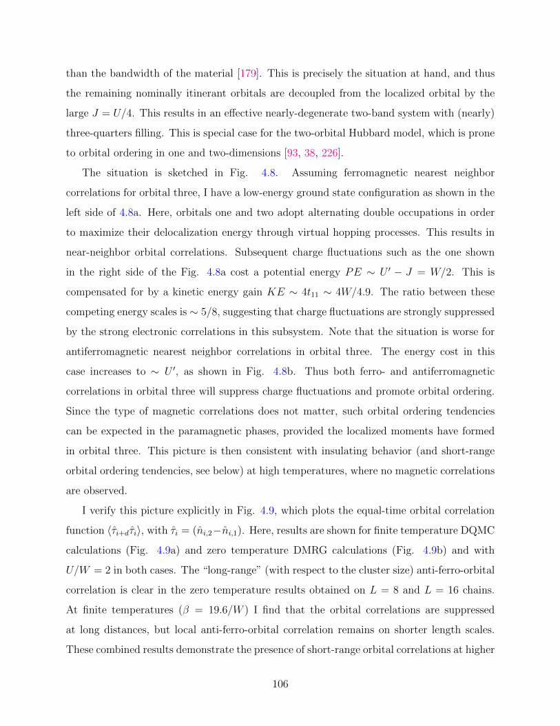
than the bandwidth of the material [179]. This is precisely the situation at hand, and thus

the remaining nominally itinerant orbitals are decoupled from the localized orbital by the

large J = U/4. This results in an effective nearly-degenerate two-band system with (nearly)

three-quarters filling. This is special case for the two-orbital Hubbard model, which is prone

to orbital ordering in one and two-dimensions [93, 38, 226].

The situation is sketched in Fig. 4.8. Assuming ferromagnetic nearest neighbor

correlations for orbital three, I have a low-energy ground state configuration as shown in the

left side of 4.8a. Here, orbitals one and two adopt alternating double occupations in order

to maximize their delocalization energy through virtual hopping processes. This results in

near-neighbor orbital correlations. Subsequent charge fluctuations such as the one shown

in the right side of the Fig. 4.8a cost a potential energy PE ∼ U ′ − J = W/2. This is

compensated for by a kinetic energy gain KE ∼ 4t11 ∼ 4W/4.9. The ratio between these

competing energy scales is ∼ 5/8, suggesting that charge fluctuations are strongly suppressed

by the strong electronic correlations in this subsystem. Note that the situation is worse for

antiferromagnetic nearest neighbor correlations in orbital three. The energy cost in this

case increases to ∼ U ′, as shown in Fig. 4.8b. Thus both ferro- and antiferromagnetic

correlations in orbital three will suppress charge fluctuations and promote orbital ordering.

Since the type of magnetic correlations does not matter, such orbital ordering tendencies

can be expected in the paramagnetic phases, provided the localized moments have formed

in orbital three. This picture is then consistent with insulating behavior (and short-range

orbital ordering tendencies, see below) at high temperatures, where no magnetic correlations

are observed.

I verify this picture explicitly in Fig. 4.9, which plots the equal-time orbital correlation

function 〈τi+dτi〉, with τi = (ni,2−ni,1). Here, results are shown for finite temperature DQMC

calculations (Fig. 4.9a) and zero temperature DMRG calculations (Fig. 4.9b) and with

U/W = 2 in both cases. The “long-range” (with respect to the cluster size) anti-ferro-orbital

correlation is clear in the zero temperature results obtained on L = 8 and L = 16 chains.

At finite temperatures (β = 19.6/W ) I find that the orbital correlations are suppressed

at long distances, but local anti-ferro-orbital correlation remains on shorter length scales.

These combined results demonstrate the presence of short-range orbital correlations at higher

106

Orb 3

Orb 2

Orb 1

i i + 1 i i + 1(a)

Orb 3

Orb 2

Orb 1

i i + 1 i i + 1(b)

PE ~ U’ - J

KE ~ t11

PE ~ U’

KE ~ t11

Figure 4.8: A cartoon sketch of the relevant charge fluctuation processes leading tothe insulating state when U/W = 2 assuming (a) ferromagnetic and (b) antiferromagneticnearest neighbor correlations within the orbital that has undergone the orbital selective Motttransition (orbital three).

107

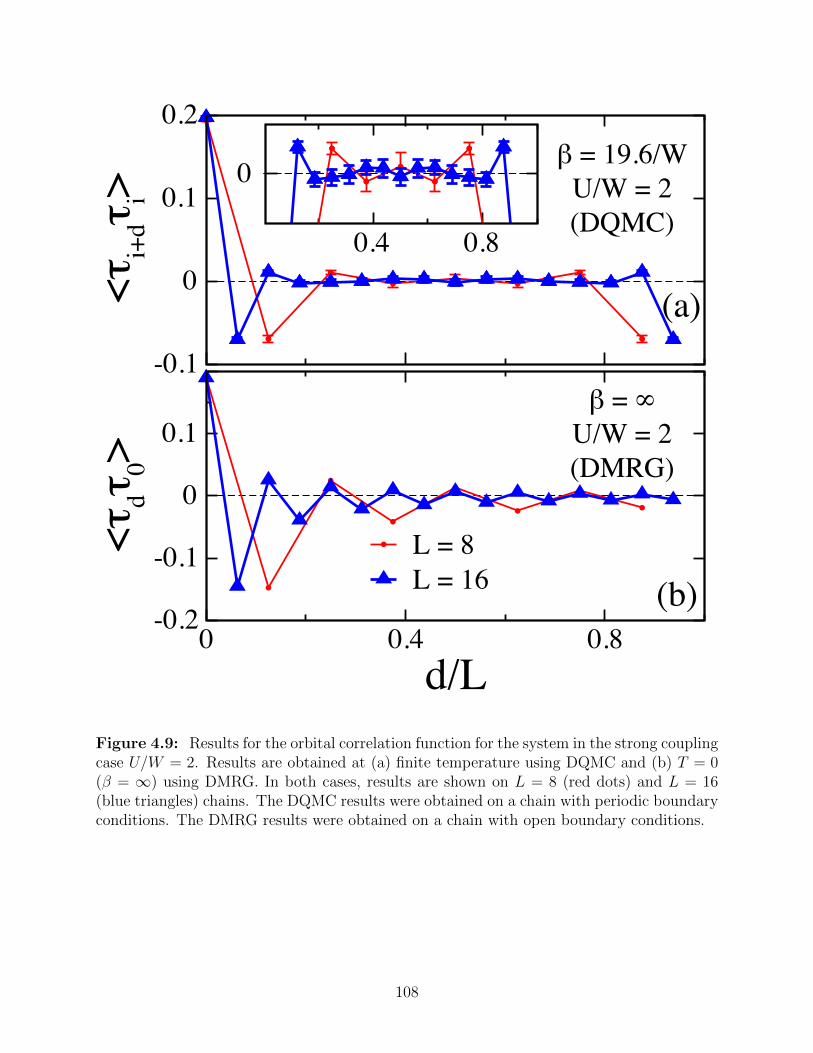
-0.1

0

0.1

0.2

(a)

` = 19.6/WU/W = 2(DQMC)

0

0.4 0.8

-0.2

-0.1

0

0.1

0 0.4 0.8d/L

(b)L = 8 L = 16

<oi+

doi>

<odo

0>

` = 'U/W = 2(DMRG)

Figure 4.9: Results for the orbital correlation function for the system in the strong couplingcase U/W = 2. Results are obtained at (a) finite temperature using DQMC and (b) T = 0(β = ∞) using DMRG. In both cases, results are shown on L = 8 (red dots) and L = 16(blue triangles) chains. The DQMC results were obtained on a chain with periodic boundaryconditions. The DMRG results were obtained on a chain with open boundary conditions.

108

temperatures, which grow in length as the temperature is decreased. The corresponding

orbitally resolved DOS are plotted in Fig. 4.10 for both cases. Both methods predict that

the system is insulating, with a charge gap width on orbitals one and two of about 0.5 eV

(estimated from half the peak-to-peak distance in the DOS). The presence of a gap at finite

temperature also confirms that the short range orbital correlations are sufficient to open a

gap in the spectral function. Finally, I stress these results will survive in the thermodynamic

limit L→∞. This is confirmed in the inset in Fig. 4.10b, which plots the T = 0 gap ∆ as

a function of chain length L, as obtained from DMRG. In this case, computing the DOS for

the longer chains is impractical. Therefore, I defined an alternative measure of the gap as

∆ = E(N + 1) + E(N − 1)− 2E(N), where E(N) is the ground state energy of the system

with N = 4L electrons. This definition agrees with the gap size obtained directly from the

DOS that was explicilty computed for the shorter chains. Using this, I find that the DMRG

gap size ∆ decreases with increasing chain lengths, until leveling off at a value of ∼ 0.2 eV

in the L→∞ limit.

4.3 Discussion and Summary

I have performed a momentum-resolved study of a multi-orbital model defined on extended

1D chains using non-perturbative DQMC and DMRG. This has allowed me to compute

the several properties of an OSMP in a momentum resolved manner without resorting to

approximate methods. I find that several properties do indeed exhibit significant momentum

dependencies, not be captured by local approximations introduced by DMFT; however, the

1D case I have considered represents the worst case for DMFT. In that sense my results

complement existing DMFT efforts by providing analysis in a region where the method is

expected to perform badly.

My results establish the hierarchy of charge and magnetic orderings in this model. At

low temperatures, the DMRG calculations (as well as those in Ref. [218]) demonstrate that

orbital three is ferromagnetically ordered at T = 0. Contrary to this, my finite temperature

DQMC calculations find no indications of any magnetic order for β < 19.6/W ; the magnetic

structure factor S(q) is completely featureless as a function of q at these temperatures.

109

0

0.4

0.8

1.2

-10 -8 -6 -4 -2 0 2

Nγ(

ω)

[sta

tes/

eV/s

pin

](a)

DQMC L = 8

orb 1

orb 2

orb 3

-0.4 0 0.4

0

0.4

0.8

1.2

-0.8 -0.4 0 0.4 0.8 1.2 1.6 2

ω (eV)

(b)DMRG L=8

orb 1

orb 2

orb 3 0.2

0.4

0 0.1

∆ (

eV

)

1/L

Figure 4.10: Results for the orbitally-resolved density of states for each orbital obtainedfor U/W = 2 and on L = 8 site chains. Panel (a) shows DQMC results at β = 19.6/Wand the inset zooms in to energy around Fermi surface. Panel (b) shows DMRG results forthe same conditons but at zero temperature (β = ∞). The inset plots a finite size scalinganalysis of the charge gap obtained within DMRG (see text). The dash line in both panelsindicates the Fermi energy.

110

Despite this, my finite T calculations find an orbital-selective Mott phase, as well as a fully

insulating phase arising due to short-range orbital ordering, depending on the strength of

the Hubbard interaction U . I therefore conclude that the charge ordering occurs before any

magnetic ordering in this model.

The results shown in Fig. 4.3d and 4.4d show that orbital three in my model, which has

the narrowest band width, undergoes a transition to a Mott phase at βW ∼ 10 − 15. This

in combination with the lack of magnetic signal means that OSMP in this parameter regime

is a true Mott phase as opposed to a Slater insulator where the insulating behavior is driven

by magnetism. My results also demonstrate that it is insufficient to identify an OSMP using

the orbital occupations only in some instances. One should be particularly careful in regions

of parameter space where the itinerant bands have average occupations close to special cases

known for one and two-orbital Hubbard models. In my case, the average fillings of the

itinerant orbitals are 〈n1〉 ∼ 1.53 and 〈n2〉 ∼ 1.47, values very close to the special case of 3/4

filling in a degenerate two-band Hubbard model. At zero temperature, the DMRG results

obtain fillings of 1.5 for each orbital.

The orbital correlations in Fig. 4.9 give some indication as to the extend of the cluster

one might need to capture these effects using embedded cluster techniques. The β = 19.6/W

results shown in Fig. 4.9a indicate that the orbital correlations extend over (at least) three

lattice sites within the error bars of my data, while at T = 0 the correlations (Fig. 4.9b)

extend over the length of the cluster. Thus, the low-temperature correlation length can be

quite long, even in 1D. Single-site mean-field approaches cannot capture these correlations

in either case. However, one might hope that DCA or cluster DMFT extensions may be able

to address the short range correlations at elevated temperatures.

Finally, I discuss my results in the context of recent experimental work. ARPES results

for AFe2As2 have found evidence that the OSMP in these materials disappears as the

temperature is lowered [276]. This behavior was explained using a slave-boson approach

and attributed to the reduced entropy in the metallic phase in comparison to the OSMP.

My results do not show this behavior, and the OSMP is found at low temperature. This

difference may be related to the differences in the dimensionality (one vs. two) or number of

orbitals (three vs. five) between the models, or the differences between my non-perturbative

111

approach and other mean-field methods. This highlights the need for continued application

of non-perturbative methods to tractable multi-orbital Hubbard models.

112

Chapter 5

The electron-phonon interaction in

correlated multi-orbital systems

In this chapter, I study the interplay between the electron-phonon interaction and the

electron-electron interaction in multi-orbital systems. Here, we consider systems both in

one dimension and infinite-dimension. In the 1D case, I used the same parameters as I used

for the electronic properties in the chapter 4. Holstein phonons are then added into the

Hamiltonian to study the phonon effect. This 1D three-orbital Hubbard-Holstein model is

studied using DQMC. In infinite-dimension, I use dynamical mean field theory (DMFT) to

study a two-orbital Hubbard-Holstein model. The key results presented in this chapter have

appeared in Ref. [149] and Ref. [151].

In recent years, many researchers have began studying electron-electron (e-e) interactions

in multiorbital systems such as the iron-based superconductors (FeSCs). In doing so, they

have discovered numerous new phenomena, including the Hund’s metal [92, 79, 71] and the

orbital-selective Mott phase (OSMP) [5, 127, 179, 276, 148], which arise from the competing

action of the electronic interactions. These concepts have helped shape our understanding of

the enigmatic properties of these materials. Despite this success, however, surprisingly little

is currently known about how competition/cooperation with other factors such as impurities

or the electron-phonon (e-ph) interaction influences these phenomena. This question is

important for our microscopic understanding of these materials, as subtle multiorbital

correlation effects can produce states that are readily affected by small perturbations.

113

In the case of the FeSCs, the e-ph interaction was ruled out as a possible pairing mediator

by early ab initio calculations [26] indicating that the total coupling strength was small, with

a dimensionless e-ph coupling λ ≤ 0.2. Because of this, many researchers have assumed that

this interaction plays a secondary role in these materials with regards to other aspects as

well. However, there is growing evidence that this outlook may have been premature. For

example, more recent calculations find that taking into account the possible magnetism

[280, 25, 48, 167] or orbital fluctuations [128, 225] can increase the total e-ph coupling

strength compared to the original estimates. This finding is consistent with the general

notion that electron correlations can enhance e-ph interactions [33]. Moreover, the discovery

of the FeSe films on oxide substrates [256] has implicated new possible lattice interactions,

either across the interface [141, 213] or within the FeSe film [47]. Since bulk FeSe is believed

to be in the OSMP regime [260, 70], these experiments naturally raise questions about when

and how e-ph interactions can influence such multi-orbital phenomena.

Hubbard-Holstein models are the simplest models capturing the interplay between e-e

and e-ph interactions. The single-band variant has been extensively studied, particularly

at half-filling, where a direct competition occurs between antiferromagnetic Mott insulating

(MI) and charge-density-wave (CDW) phases [14, 15, 20, 196, 188, 264, 227, 163, 193, 121].

In comparison, far fewer studies exist for multiband generalizations of the model [272, 128].

Motivated by this, I study the interplay between the e-e and e-ph in the multiorbital

Hubbard-Holstein model. In particular, I use DMFT [78] to study the inifinite-dimensional

case, since DMFT can give an exact solution in this case. Also, I use DQMC to study the

one-dimensional case in that DMFT fails to produce exact solutions in low dimensions.

5.1 The infinite-dimensional case

I first study the interplay between the e-e and e-ph interactions in the degenerate two-

orbital Hubbard-Holstein model in infinite-dimension. The Hamiltonian for this model [272]

is H = Hkin +Hlat +He−ph +He−e, where

Hkin = −∑〈i,j〉,γ,σ

tγc†i,γ,σcj,γ,σ − µ

∑i,γ,σ

ni,γ,σ,

114

He−ph +Hlat = g∑i,γ,σ

(b†i + bi

)(ni,γ,σ −

1

2

)+ Ω

∑i

b†ibi ,

He−e = U∑i,γ

ni,γ,↑ni,γ,↓ + U ′∑i,γ 6=γ′

ni,γ↑ni,γ′,↓

+(U ′ − J)∑

i,γ<γ′,σ

ni,γ,σni,γ′,σ

+J∑i,γ 6=γ′

(c†i,γ,↑c†i,γ,↓ci,γ′,↓ci,γ′,↑ − c

†i,γ,↑ci,γ,↓c

†i,γ′,↓ci,γ′,↑)

Here, 〈· · · 〉 denotes a summation over nearest neighbors; c†i,γ,σ creates an electron with spin

σ in orbital γ = 1, 2 on site i; b†i creates a phonon on site i; ni,γ,σ = c†i,γ,σci,γ,σ is the particle

number operator; tγ is the nearest neighbor hopping integral for orbital γ; U and U ′ are the

intra- and inter-orbital Hubbard interactions, respectively. Throughout, I choose U ′ = U−2J

due to rotational symmetry [78, 36]. J is the Hund’s coupling, which is fixed to J = U/5

unless otherwise stated; g is the e-ph interaction strength; Ω is the phonon energy; and µ is

the chemical potential, which is adjusted to fix the average particle per site to 〈n〉 = 2.

I work in infinite dimensions (where DMFT is exact) by adopting a Bethe lattice with a

semi-circular density of states ργ(ε) = 8πW 2

γ

√(Wγ/2)2 − ε2, where Wγ = 4tγ is the bandwidth.

Throughout this chapter, I set W1 = 5W2 ≡ W = 2 eV, fix the temperature at T = 1β

= 0.01

eV, unless otherwise stated, and set the phonon energy to Ω = 0.15 eV. The bandwidth

and Hund’s coupling J are chosen so that I can obtain a robust OSMP without the e-ph

coupling. The dimensionless e-ph coupling constant is defined as λ = 2g2

WΩ. The impurity

model is solved using the exact diagonalization and the infinite phonon Hilbert space is

limited by only allowing up to Nph phonons, where Nph ∼ 40 is typical, depending on the

parameters used. I have checked that all of my results are well converged for increasing

values of Nph.

The convergence of quasiparticle weight with bath size Nb is shown in Fig. 5.1, where

Fig. 5.1(a) and 5.1(b) are results of λ = 0 and U = 0, respectively. Both Fig. 5.1(a) and

5.1(b) show that phase transition critical values are consistent for Nb = 4 and Nb = 6. There

is a slight difference between Nb = 4 and Nb = 6 for Z1, while results of Z2 are very close.

Hence, Nb = 4 is enough to produce reliable solutions for the two-orbital model. To reduce

the total computational demands, I use Nb = 4 in the following calculations.

115

0

0.2

0.4

0.6

0.8

1

0 0.5 1 1.5 2

Zγ

U (eV)

λ = 0

(a)

Z1 (Nb = 4)

Z2 (Nb = 4)

Z1 (Nb = 6)

Z2 (Nb = 6)

0 0.05 0.1 0.15 0.2λ

U = 0 eV

(b)

Z1 (Nb = 4)

Z2 (Nb = 4)

Z1 (Nb = 6)

Z2 (Nb = 6)

Figure 5.1: (color online) Convergence of quasiparticle weight Zγ with bath size Nb. Solidlines and points are results of Nb = 4 and Nb = 6, respectively. In panel (a) λ = 0 and inpanel (b) U = 0 eV.

116

5.1.1 Competition between U and λ

The λ-U phase diagram for the model is shown in Fig. 5.2. Here, I plot the orbitally

resolved Matsubara quasiparticle weight Zγ =(

1− ImΣ(iπT )πT

)−1

on a logarithmic scale. The

quasiparticle weight Zγ approaches to 1 when it is metallic, while Zγ approaches to 0 when it

is insulating. Five distinct phases can be identified from the values of Zγ, the local magnetic

moment m2γz = 〈(nγ↑ − nγ↓)2〉, and the average number of phonon quanta Nph = 〈b†b〉 (all

shown in Fig. 5.3), and their boundaries are indicated by the white lines. Three of these

phases are similar to those found in the single-band Hubbard-Holstein model. The first

phase is a metallic phase (M) at small (λ, U), where both Z1 and Z2 are large. The second

is a Mott insulating (MI) phase, which appears at large U . It is identified by a situation

where Z1 = Z2 = 0, the magnetic moments are large m21,z ≈ m2

2,z ≈ 1, and Nph is nearly

zero. The third phase is a CDW insulating phase where Z1 = Z2 = 0, while Nph is large

(Nph 1) and no local moments have formed (i.e. m21,z ≈ m2

2,z ≈ 0). An examination of the

wavefunctions reveals that the CDW phase corresponds to a state where the impurity site is

either fully occupied or entirely empty with equal probability, consistent with a checkerboard-

type ordering common to the single-band model [196, 15, 14]. This phase is likely to be a

(π, π, ...) CDW order (sometimes referred to as a strong coupling bi-polaronic insulating

phase in the single-band case). Alternatively, this phase could also reflect phase separation,

although delocalization effects should favor the CDW. Further studies on extended clusters

will be needed to address this issue.

In addition to the “standard” phases, I also observe two distinct phases with orbital

selective characteristics. The first is the widely studied OSMP, which appears between

the M and MI phases. It resembles the same OSMP found in the model without e-ph

interactions [177]. Here, the orbital with the narrower bandwidth becomes insulating with

Z2 = 0 and m22z ≈ 1, while the orbital with the wider bandwidth remains itinerant with a

non-zero quasiparticle weight. Interestingly, I also observe a second region of orbital selective

behavior, located in a small portion of parameter space between the M/OSMP phases and

the fully insulating CDW phase, denoted as OSPI in Fig. 1. As with the OSMP, in this

region, the narrow band becomes insulating while the wide band remains itinerant with

117

Figure 5.2: (color online) The phase diagram for the two-orbital Hubbard-Holstein model inthe e-ph interaction strength (λ) - Hubbard U plane at charge density n = 2 and temperatureβ = 200/W . (a) and (b) show density plots of quasiparticle weights Z1 and Z2 on alogarithmic scale, respectively. The different phases are labeled as follows: metal (M),orbital-selective Mott phase (OSMP), Mott insulater (MI), charge density wave (CDW),and orbital-selective Peierls insulator (OSPI). The white dots indicate points where thecalculations were performed, and I plotted them to show phases boundaries. The color scaleis plotted using a linear interpolation.

118

0

0.2

0.4

0.6

0.8

1

Z1

(a) U = 0.0 eVU = 0.4 eVU = 0.8 eVU = 1.1 eVU = 1.8 eVU = 2.5 eV

0

0.2

0.4

0.6

0.8

1Z

2

(b)

0

0.2

0.4

0.6

0.8

1

m1

z2

(c)

0

0.2

0.4

0.6

0.8

1

m2

z2

(d)

0

5

10

15

20

0 0.2 0.4 0.6 0.8

Np

h

λ

(e)

Figure 5.3: (color online) The quasiparticle weights (a) Z1 and (b) Z2 as a function ofthe e-ph interaction strength (λ) at different Hubbard U values. Mean values of the localmagnetic moments m2

1z, m22z and phonon numbers (Nph) are shown in (c), (d), and (e),

respectively.

119

Z1 6= 0 and Z2 = 0. But unlike the OSMP, here I find tiny local moments on orbital 2 with

m22z ≤ 0.05, and a large Nph (Nph > 1). The latter indicates the presence of a sizable lattice

distortion. The e-ph interaction drives the orbital-selective insulating properties in this case

rather than the Hubbard and Hund’s interaction. I label this state an orbital selective Peierls

insulator (OSPI), in analogy to the OSMP.

For reference, Fig. 5.3 shows the evolution of the quantities used to identify the five

regions of the phase diagram as a function of λ for different values of U . When U ≤ 0.4 eV,

m2γz and Nph vary smoothly near the phase transition, while for U > 0.4 eV, these quantities

vary quickly in the transition region, but are nevertheless continuous. This behavior is

consistent with a previous DMFT study of the single band Hubbard-Holstein model [15],

where a smooth transition occurs at weak coupling that becomes increasingly sharp as U/W

increases.

5.1.2 Hysteresis

To study the analogy between the OSMP and the OSPI further, I examine the classification of

the phase transitions and their possible hysteresis behavior [153]. Fig. 5.4(a) and 5.4(b) plot

the evolution of Zγ at T = 0.002 eV along the (U, λ = 0) and (U = 0, λ) axes, respectively.

Along the (U, λ = 0) line, there are two Mott transitions in the two-orbital system, I observe

a single hysteresis loop near the OSMP boundary, which indicates a coexistence region,

as discussed in Ref. [153]. The critical U values for increasing and decreasing interaction

strengths are Uc,1 = 0.6 eV and Uc,2 = 0.5 eV, respectively. Similarly, along the (U = 0, λ)

line I also find a single coexistence region, consistent with DMFT studies for the single band

Holstein model [184, 109]. As with the Mott transition, the hysteresis loop appears close to

the first Peierls transition and the critical λ values for increasing and decreasing interactions

are λc,1 = 0.08 and λc,2 = 0.066, respectively. Thus, the OSMP and OSPI transitions

phenomena appear to be analogous to one another. The appearance of hysteresis indicates

a first order transition out of the metallic phase while the other transitions are continuous.

Finally, I note that the hysteresis behavior disappears at T = 0.01 eV, where I performed

most of my calculations.

120

0

0.2

0.4

0.6

0.8

0.3 0.4 0.5 0.6 0.7 0.8

Zγ

U (eV)

λ = 0

(a)

Z

1

Z

2

Z-

1

Z-

2

0

0.2

0.4

0.6

0.8

0.04 0.06 0.08 0.1

Zγ

λ

U = 0 eV

(b)

Figure 5.4: (color online) (a) The quasiparticle weight Zγ as a function of U at a fixedλ = 0. (b) The quasiparticle weight Zγ as a function of λ at a fixed U = 0. Zγ are resultsat T = 0.002 eV and Zγ are results at T = 0.01 eV. The solid lines and the dashed lines areresults of increasing and decreasing U or λ, respectively.

121

5.1.3 Interplay between λ and Hund’s coupling

The Hund’s coupling plays a major role in establishing the boundaries of the OSMP [127,

180]. Therefore, I explored its role in determining the CDW and OSPI phases observed here.

Fig. 5.5 shows the phase diagram in the λ - J/U plane for a fixed U = 0.8 eV. For λ < 0.3,

the metallic phase survives to larger values of J/U as λ increases. This result is consistent

with the notion that the e-ph interaction mediates an effective attractive interaction that

competes with the onsite Hubbard interactions. When 0.3 < λ < 0.4, the OSMP disappears

and is replaced by the OSPI and CDW phases and the critical λ value for both phases is

decreased as J/U increases. For larger λ, the CDW phase persists for all J/U values. Thus,

the Hund’s coupling not only favors the OSMP transition but also has a stabilizing effect

for the lattice-driven phases.

To gain further insight into the influence of J on the OSPI phase transition, I examined

the phase transition from the metallic state to the CDW at a fixed U = 0.8 and λ = 0.384,

as shown in Fig. 5.6(a) and 5.6(b). Fig. 5.6 (a) shows quasiparticle weights Z1 and Z2 as a

function of J/U . The dashed lines are the boundaries of each phase.

On the impurity site, the electronic subspace of the ground state at half-filling can be

written as

|ψ〉 = P1 (|0000〉+ |1111〉) +

P2 (|1000〉+ |0100〉+ |1011〉+ |0111〉) +

P3 (|0010〉+ |0001〉+ |1101〉+ |1110〉) +

P4 (|1100〉+ |0011〉) + P5 (|1010〉+ |0101〉) +

P6 (|1001〉+ |0110〉) ,

in which |n1,↑n1,↓n2,↑n2,↓〉 are the basis elements for the electronic subspace and nγ,σ is the

electron number for the orbital γ and spin σ. Here, I only need six distinct coefficients Pi

due to the particle-hole symmetry of the underlying Hamiltoniain. For example, the weight

for the basis states |0000〉 and |1111〉 must be the same and equal P1.

122

Figure 5.5: (color online) The phase diagram in the λ-J/U plane at filling n = 2. (a) and(b) plot quasiparticle weights Z1 and Z2, respectively. The labels used in this graph are thesame as in Fig. 5.2. The Coulomb interaction is fixed at U = 0.8 eV and U ′ = U − 2J .The white dots indicate points where the calculations were performed, and I plotted themto show phases boundaries. The color scale is plotted using a linear interpolation.

123

0

0.1

0.2

0.3

0.4

0.5

0.6

0.7Z

γ

M OSPI CDW

U’ = U-2J

(a)

Z1Z2

0

0.1

0.2

0.3

0.4

0 0.05 0.1 0.15 0.2 0.25 0.3

|Pn|2

J/U

(b)

U’ = U

U = 0.8

λ = 0.382

(c)

0 0.05 0.1 0.15 0.2 0.25 0.3

J/U

(d)

|P1|2

|P2|2

|P3|2

|P4|2

|P5|2

|P6|2

Figure 5.6: (color online) (a) and (c) plot the quasiparticle weights Z1 and Z2 vs. J/U .(b) and (d) plot the probabilities |Pi|2 of the eight states mentioned in the text vs. J/U .The interorbital repulsion is fixed to U ′ = U − 2J in (a) and (b). In (c) and (d) U ′ = U .The Hubbard interaction strength is U = 0.8 eV and e-ph interaction strength is λ = 0.384in all panels. The dashed lines in (a) and (b) correspond to phase boundaries.

124

In a pure CDW phase composed of fully occupied and empty sites one has P1 = 1√2

and

Pn = 0 for n = 2, ..., 6. This ground state produces 〈nγ,σnγ′,σ′〉 = 0.5, where γ (γ′) = 1 or 2

and σ (σ′) =↑ or ↓. In a cluster system, the two bases |0000〉 and |1111〉 should be arranged

on alternating lattice sites to minimize the kinetic energy of the system. This arrangement

corresponds to a CDW with ordering vector Q = π in 1D, (π, π) in 2D, (π, π, π) in 3D,

etc.. The value of the six probabilities for each state as a function of J/U is plotted in Fig.

5.6(b). Near the phase transition from the metallic state to the OSPI, P1 increases quickly,

which implies that the state (|0000〉+ |1111〉) has a lower energy and is being preferentially

populated. This energy reduction is achieved by decreasing the effective e-e interaction via

the e-ph interaction, such as Ueff = U + 2λWγ

ω2/Ω2−1. In addition, U ′ is also renormalized by

the e-ph interaction via U ′eff = U ′ − 2λW in the limit of Ω → ∞. When U ′eff − J < 0 and

the attraction potential between two orbitals can compensate the energy cost for double

occupation on the individual orbitals, thus stabilizing the CDW state. Hence, in the multi-

orbital case, the stabilization of the CDW phase with increasing J/U is due to the reduction

of the interorbital Hubbard interaction, imposed by the condition that U ′ = U − 2J . In

short, increasing J reduces U ′ and therefore also reduces the total potential energy cost for

a double occupation of a given site. The cost for creating a charge ordered phase, where

each site alternates between fully occupied and empty, is therefore lowered. To confirm

my arguments, I fix U ′ = U and use the same U and λ values to calculate Zγ and P 2n in

Fig. 5.6(c) and 5.6(d), respectively. In this case, neither the CDW nor the OSPI phase

are found because the fixed U ′ prevents U ′eff − J from becoming negative at an intermediate

λ. For larger large λ values both the OSPI and CDW phases appear; however, their phase

boundaries are largely independent of J/U when U = U ′.

5.2 The one dimensional case

The prior study was carried out in infinite dimensions, where DMFT is exact; however, given

the dependence on dimensionality found for the single-orbital HH model [44, 15, 196], it is

essential to study the problem in other dimensions, as a function of doping, and with different

techniques. Motivated by this, I present here a complementary study of the three-orbital

125

HH model defined on an extended 1D chain at an average electron filling 〈n〉 = 4. I study

the model using DQMC, which is a nonperturbative auxiliary-field technique and capable of

handling both the e-e and e-ph interactions on equal footing.

My starting point is a simplified one-dimensional three-orbital Hubbard model as shown

in chapter 4. I then add a Holstein-type interaction, where the atomic displacement is coupled

to the electron density on each orbital. The full Hamiltonian is H = H0+He−e+Hlat+He−ph,

where

H0 = −∑〈i,j〉σ,γ,γ′

tγγ′c†i,γ,σcj,γ′,σ +

∑i,σ,γ

(∆γ − µ)ni,γ,σ (5.1)

are the non-interacting electronic terms,

Hlat =∑i

[P 2i

2M+MΩ2

2X2i

]= Ω

∑i

(b†ibi +

1

2

)(5.2)

are the noninteracting lattice terms,

He−e = U∑i,γ

ni,γ,↑ni,γ,↓ +

(U ′ − J

2

)∑i,σ,σ′

γ<γ′

ni,γ,σni,γ,σ′

+J∑i,γ<γ′

Szi,γSzi,γ′ (5.3)

are the on-site Hubbard and Hund’s interaction terms, and

He−ph = α∑i,γ,σ

Xini,γ,σ = g∑i,γ,σ

(b†i + bi

)ni,γ,σ (5.4)

are the e-ph coupling terms. Here, 〈. . . 〉 denotes a sum over nearest neighbors; c†i,γ,σ (ci,γ,σ)

creates (annihilates) a spin σ electron in orbital γ = 1, 2, 3 on site i; b†i (bi ) creates

(annihilates) a phonon on lattice site i; Szi,γ is the z-component of the spin operator Si,γ;

ni,γ,σ = c†i,γ,σci,γ,σ is the number operator; and Xi and Pi are the lattice position and

momentum operators, respectively. The parameters ∆γ are the on-site energies for each

orbital; tγ,γ′ are the intra- and interorbital hopping integrals; U and U ′ are the intra- and

126

interorbital Hubbard interactions, respectively, and J is the Hund’s coupling. The parameter

g = α√

2MΩ is the strength of the e-ph coupling and Ω is the phonon energy. Finally, µ is

the chemical potential, which fixes the average particle number.

In Eq. (5.3) I have neglected the pair-hopping and spin-flip terms of the Hunds

interaction, as was done in Ref. [148] for the same model without e-ph interactions. These

terms introduce a significant Fermion sign problem [157] for DQMC calculations and are

therefore neglected to make the problem tractable. Prior work [156] has shown that these

terms only change the location of the various phase boundaries for the model considered

here in the absence of the e-ph interaction. I, therefore, proceed assuming that this will also

hold true once the phonons are included in calculations.

Throughout this work, I choose U ′ = U − 2J , as is standard for enforcing rotational

symmetry [36], although I have neglected the pair hopping and spin-flip terms in Eq. (5.3).

I further vary U while holding J = U/4 fixed. This choice produces a robust OSMP [218, 156,

148] in the absence the e-ph interaction and is appropriate for the FeSCs. I work at a fixed

filling 〈n〉 = 4, which is typical for three-orbital Hubbard models used to describe the 2D

FeSCs with two hole pockets near the Γ point and one electron pocket near the X (Y ) point

[55]. I expect that the same filling is needed to describe the quasi-one-dimensional system

BaFe2S3. This choice of filling also allows us to make direct comparisons to previous studies

in the absence of the e-ph interaction [218, 156, 148], such as the one presented in chapter

4. In this spirit, I also set t11 = t22 = −0.5 eV, t33 = −0.15 eV, t13 = t23 = 0.1 eV, t12 = 0

eV, ∆1 = −0.1 eV, ∆2 = 0 eV, ∆ = 0.8 eV, and Ω = 0.5 eV, again following Refs. [148] and

[218]. The total bandwidth of the non-interacting model is W = 2.45 eV, which serves as

the unit energy in the following calculations. The dimensionless e-ph coupling constant is

defined as λ = α2/(MΩ2W ). (Note that since this is a multi-band system, different choices

of bandwidths are possible. Here, I select the total bandwidth, as was done for the infinite-

dimensional case.) Finally, I set a = M = 1 as units of distance and mass, respectively, and

work at an inverse temperature β = 14.7/W unless stated otherwise; this temperature is low

enough to identify the ordering tendencies in the model.

I use DQMC to solve the 1D three-orbital HH model. Throughout this work, I use

a one-dimensional chain with a chain size N = 16 and imaginary time discretization of

127

∆τ = 0.245/W , unless otherwise stated. In all of simulations, I have not observed significant

∆τ errors introduced by this choice.

The main results are summarized in Fig. 5.7, which provides a schematic of the phase

diagram of the model. I find four distinct regions in the λ − U parameter space, including

states with metallic (M) characteristics, an OSMP region, a CDW order, and a region with

strong orbital correlations (OC) and insulating characteristics. Comparing with the infinite-

dimensional case, I find a new phase, namely OC state, but fail to produce the OSPI phase in

the one-dimensional case. The details of these four phases will be discussed in the following

sections.

5.2.1 Weak Electron-Phonon Coupling

In chapter 4 I presented that the model without phonons showed that an OSMP forms for U

values in the range 0.6 < U/W < 2 for my choice of J . In this state, orbital three becomes

insulating while the remaining orbitals host itinerant electrons [218, 156]. The onset of this

phase is signaled by the fact that the filling on orbital three 〈n3〉 = 1. For U/W > 2, orbitals

1 and 2 retain a noninteger filling but are driven into an insulating state by the onset of

short-range orbital ordering [148]. To avoid this complication, I restrict U/W < 1.

I now examine the impact of the e-ph interaction on the OSMP. Figure 5.8 plots the

electronic occupations of the three orbitals for different values of U/W and λ. For λ = 0,

Fig. 5.8(c) shows that 〈n3〉 converges to 1 as U/W increases, implying that a Mott gap is

formed on this orbital for U/W ≥ 0.4. At the same time, 〈n1〉 and 〈n2〉 maintain noninteger

values, implying that these orbitals remain itinerant [see Fig. 5.8(a) and 5.8(b)]. These

results are consistent with previous studies [218, 156]. When I include the e-ph coupling,

the orbital occupations are modified significantly. For example, Figs. 5.8(d) - 5.8(f) show

that the e-ph coupling tends to make electronic occupations on all three orbitals uniform

when U/W < 0.4, with the average filling on each orbital approaching 〈ni〉 = 43

when λ is

large. This value of the occupation on each orbital is consistent with a chagre-ordered state

where two sites are fully occupied and one site is empty, which is shown in the CDW region

of Fig. 5.7. This kind of charge order arises from the attractive interaction mediated by the

e-ph interaction. For the fully occupied site, the attractive interaction can be mapped into

128

Figure 5.7: (color online) A sketch of the λ-U phase diagram for the model as inferredfrom DQMC calculations. Four distinct regions are found, which include states with metallic(M) characteristics, an orbital-selective Mott region (OSMP), a charge-density-wave (CDW)order, and a region with strong orbital correlations (OC) and insulating characteristics. Thelevel diagrams sketch the dominant electronic configurations in each region. Here, W denotesthe electronic bandwidth.

129

6 = 0:006 = 0:066 = 0:156 = 0:18

6 = 0:216 = 0:336 = 0:41

1.3

1.4

1.5

1.6

n1

(a)

1.3

1.4

1.5

n2

(b)

0 0.4 0.8U=W

0.8

1

1.2

1.4

n3

(c)

U=W = 0:0U=W = 0:1U=W = 0:2U=W = 0:4

U=W = 0:6U=W = 0:8U=W = 1:0

(d)

(e)

0 0.2 0.46

(f)

Figure 5.8: (color online) The variation of electronic densities on the three orbitals asa function of the Hubbard U and the e-ph coupling strength λ. Panels (a) - (c) show thevariation of electronic densities as a function of the Hubbard U on orbitals γ = 1, 2, and 3,respectively. Similarly, panels (d) - (f) show the change of electronic densities as a functionof λ on the same three orbitals. In each panel, error bars smaller than the marker size havebeen suppressed for clarity, and a smoothing spline used as a guide to the eye.

130

a negative effective U for all three orbitals at this site in the large-Ω limit. For an empty

site, the effective interaction is not modified by the e-ph coupling. Therefore, the effective

Hubbard interaction is not uniform in real space if there is a density modulation. When the

e-ph coupling is strong, this nonuniform attractive interaction can produce a charge-ordered

state but with a uniform average occupation on each orbital. The transition from a CDW

phase to an OSMP can be seen in Fig. 5.8(c), where n3 decreases from 43

to 1 at λ = 0.33.

Increasing the e-ph coupling pushes this transition to larger values of U/W ; for example, for

λ = 0.41 it occurs at U/W ∼ 0.5.

The competition between the CDW and OSMP tendencies is also manifest in the behavior

of each orbital’s double occupation Dγ = 〈nγ,↑nγ,↓〉−〈nγ,↑〉〈nγ,↓〉, as summarized in Fig. 5.9.

When the phonon-mediated effective attraction overcomes the Coulomb repulsion, I expect

Dγ > 0; otherwise, Dγ < 0. Figures 5.9(a)-5.9(c) present Dγ as a function of U/W for fixed

values of λ, where I find that Dγ decreases as U is increased, and D3 converges to −14

in the

limit of a strong Hubbard interaction, consistent with a Mott insulating state where double

occupation is suppressed. Figs. 5.9(d)-5.9(f) alternatively plot the data as a function of λ

for fixed values of U/W . Here, I find that for U/W < 0.4, Dγ increases as λ increases and

converges to 29

on each orbital. This value is consistent with the double occupations expected

for the CDW phase shown in Fig. 5.7.

The electronic density and double occupations provide indirect evidence of the CDW

phase. To obtain more direct evidence of a CDW order, I calculated the charge susceptibility

χcγ,γ′(q) =1

N

∫ β

0

dτ〈nq,γ(τ)nq,γ′(0)〉, (5.5)

where q is the momentum, τ is the imaginary time, nq,γ =∑

i,σ eiqrini,γ,σ, and ri is the lattice

vector.

Figure 5.10 shows the momentum dependence of the three intraorbital charge suscepti-

bilities for U/W = 0 and different e-ph coupling strengths. At weak coupling (i.e. λ = 0.0

and λ = 0.06), χcγ,γ(q) is small, with no clear peak at any momenta. This observation implies

that a finite value of λ is needed for charge correlations to develop at this temperature, and is

consistent with the one-dimensional Holstein model [90]. As the value of λ is increased, a clear

131

6 = 0:006 = 0:066 = 0:156 = 0:18

6 = 0:216 = 0:336 = 0:41

0

0.1

0.2

D1

(a)

0

0.1

0.2

D2

(b)

0 0.4 0.8U=W

-0.2

-0.1

0

0.1

0.2

D3

(c)

U=W = 0:0U=W = 0:1U=W = 0:2U=W = 0:4

U=W = 0:6U=W = 0:8U=W = 1:0

(d)

(e)

0 0.2 0.46

(f)

Figure 5.9: (color online) The variation of double occupancies on the three orbitals as afunction of the Hubbard U and the e-ph coupling strengths λ. Panel (a) - (c) shows thevariation of double occupancies as a function of the Hubbard U on orbitals γ = 1, 2, and 3,respectively. Similarly, panels (d) - (f) show the change of double occupancies as a functionof λ on the same three orbitals. In each panel, error bars smaller than the marker size havebeen suppressed for clarity, and a smoothing spline is used as a guide to the eye.

132

0

5

10

15

20

@c 11

(a)

U=W = 0

6 = 0:00

6 = 0:06

6 = 0:15

6 = 0:18

6 = 0:33

6 = 0:41

0

5

10

15

20

@c 22

(b)

0 0.2 0.4 0.6 0.8 1q(:=a)

0

5

10

15

20

@c 33

(c)

Figure 5.10: (color online) Momentum dependence of the charge correlation functionχcγ,γ(k) for orbtial 1 (a), orbital 2 (b), and orbital 3 (c) at different λ values. The HubbardU/W = 0. In each panel, error bars smaller than the marker size have been suppressed forclarity.

133

peak structure forms in χcγγ(q). For instance, already at λ = 0.18 I find a peak centered at

q = π/a for all three orbitals, indicating the formation of a two-sublattice charge correlation

at this simulation temperature (β = 14.7/W ). Upon further cooling of the system, I find

that additional charge correlations develop at a second q point. For example, Fig. 5.11

compares χcγ,γ(q) at β = 14.7/W and β = 49/W for the λ = 0.15 and U/W = 0 case. For

temperature β = 14.7/W , χcγ,γ(q) has a single peak at q = π/a; however, as the temperature

is decreased to β = 49/W , χcγ,γ(q) increases and a second peak forms q ∼ 2π/3 − 3π/4,

which is evident as a shoulder in χcγ,γ(q). To better recognize these two peaks, I plot as a

guide-to-the-eye the sum of two Lorentzian functions centered at q = 2π/3a (dash-dotted

line) and q = π/a (dotted line).

The two peak structures in χcγ,γ(q) likely reflect different ordering tendencies. The charge

configurations sketched in Fig. 5.7 are consistent with q1 ≈ 2π/3a and q2 = π/a orderings. I

propose, therefore, that the CDW state is characterized by a superposition of | . . . 660660 . . . 〉

and | . . . 606660〉 configurations along the chain, where the number indicates the number of

carriers on each site. These charge configurations are also consistent with the values of

the orbitally-resolved single and double occupancies discussed previously. In fact, these two

peaks reflect two different values of 2kF that appear in this multiorbital model; The Fermi

momentum for orbitals 1 and 2 is ∼ 0.33π/a, while the Fermi momentum for orbital 3 is

∼ 0.5π/a. Thus, these two peak values correspond to q = 2kF in the weak-coupling limit,

where the CDW tendencies are driven primarily by nesting conditions. When I increase the

e-ph coupling further, the kF for orbitals 1 and 2 increases to 0.5π/a. Therefore, I expect

that only one peak will be observed in the charge-denstiy-wave susceptibility in the limit of

strong e-ph coupling.

I now turn to the spectral weight of the three orbitals in the vicinity of the Fermi level

EF to assess whether the various phases I observe are insulating or not. The spectral weight

can be estimated directly from the imaginary-time Green’s function using the relationship

[248]

βGγ(r = 0, β/2) = β∑k

∫dω sech(βω/2)Aγ(k, ω), (5.6)

134

0

10

20

30

40

@c 11

(a)U=W = 0 6 = 0:15

- = 14:7=W

- = 49=W

0

10

20

30

40

@c 22

(b)

0 0.2 0.4 0.6 0.8 1q(:=a)

0

20

40

60

@c 33

(c)

Figure 5.11: (color online) Momentum dependence of the charge correlation functionχcγ,γ(q) for orbtial 1 (a), orbital 2 (b), and orbital 3 (c) at different β values. The HubbardU/W = 0 and λ = 0.15. The black dashed lines are eye-guided lines for a combination of twoLorentzian functions with different peak positions. The two Lorentzian functions are shownwith dotted and dash-dotted lines, respectively. In each panel, error bars smaller than themarker size have been suppressed for clarity.

135

where Aγ(k, ω) is the orbitally resolved spectral function. At low temperature, the function

βsech(βω/2) is sharply peaked around ω = EF = 0 and thus provides a measure of the

spectral weight integrated within a window of a few β−1 of EF.

Figure 5.12 plots βGγ(r = 0, β/2) for the three orbitals for different values of U/W and

λ. In Figs. 5.12(a)-5.12(c), the spectral weight of each orbital is plotted as a function of

U for fixed λ. In the absence of the e-ph interaction (λ = 0), the spectral weight of all

three orbitals decreases as the Hubbard U is increased. However, the spectral weight on

orbital γ = 3 decreases much more rapidly than the other two orbitals, consistent with the

formation of an OSMP [148]. [The small but nonzero value of βG3(r = 0, β/2) is due to the

elevated temperature of the simulation.] As the value of λ increases, I begin to see the loss

of spectral weight in all three orbitals when U/W is small.

Fig. 5.12(d)-5.12(f) plot βGγ(r = 0, β/2) as a function of λ for fixed U/W . For U/W = 0,

the spectral weight of all three orbitals is suppressed as the e-ph coupling is increased. I

further observe a sudden decrease in the spectral weight of all three orbitals for λ ≥ 0.15,

where a prominent peak in χcγ,γ(k) is observed. Thus, for λ ≥ 0.15 and U/W = 0, the system

is an insulating state driven by CDW correlations. The behavior of the spectral weight is

qualitatively similar for U/W < 0.2, however the transition to the CDW phase occurs at

larger values of λ as U/W increases. Based on these results, I conclude that the CDW phase

appearing at large λ is insulating.

Unlike the OSMP, I do not find any orbital-selective behavior associated with the

formation of the CDW phase; the rate at which the spectral weight approaches zero appears

to be the same for all three orbitals at this temperature. This result is in contrast to the

degenerate two-orbital case with inequivalent bandwidths [149], where orbital-selective CDW

behavior was found. This difference could be attributed to changes in the total bandwidth,

dimensionality, or model. (For example, the current model has inequivalent bandwidths and

crystal-field splittings while the former only had inequivalent bandwidths.) Further studies

will be needed to better understand the differences between these two cases.

I now return to the competition between the OSMP and CDW phases. Figures 5.12(a)-

(c) reveal that the spectral weight decreases as the strength of the e-ph is increased when

U/W is small. For a fixed value of λ 6= 0, βGγ(r = 0, β/2) initially increases with U/W ,

136

6 = 0:006 = 0:066 = 0:156 = 0:18

6 = 0:216 = 0:336 = 0:41

0

0.5

1

-G

11(r

=0;-=2

) (a)

0

0.5

1

-G

22(r

=0;-=2

)

(b)

0 0.4 0.8U=W

0

1

2

-G

33(r

=0;-=2

) (c)

U=W = 0:0U=W = 0:1U=W = 0:2U=W = 0:4

U=W = 0:6U=W = 0:8U=W = 1:0

(d)

(e)

0 0.2 0.46

(f)

Figure 5.12: (color online) The variation of the spectral weights for the three orbitals asa function of the Hubbard U and the e-ph coupling strength λ. Panels (a) - (c) show thevariation of spectral weights as a function of the Hubbard U for three orbitals, respectively.Panels (d) - (f) show the change of spectral weights as a function of λ for three orbitals,respectively. In each panel, error bars smaller than the marker size have been suppressed forclarity, and a smoothing spline is used as a guideline to the eye.

137

before reaching a maximum value and decreases along the U axis. This behavior reflects the

competition between the e-ph and the e-e interactions. At small U/W the CDW correlations

dominate, for large U/W the OSMP correlations dominate, and for intermediate values of λ

a metallic phase is realized.

5.2.2 Spectral properties of the CDW phase

The spectral function of the OSMP was studied in detail in chapter 4 in the absence of e-ph

interactions. I will focus, therefore, on the spectral function of the CDW phase. Figure 5.13

shows the spectral function for U = 0 and λ = 0.33 and the orbitally-resolved components.

The system is insulating, with a large CDW gap and broadened spectral features, consistent

with the spectral weight analysis. The upper bands of three orbitals have dispersions with

a clear folded shape, while the lower bands of orbitals 1 and 2 have a more cosine-like

dispersion. This cosinelike shape arises from the combination of an incoherent peak and

an additional peak arising from thermally activated transitions to states with additional

phonons excited [99]. To better recognize these two peaks, Figs. 5.13(e) - 5.13(l) plot the

spectral functions at fixed momentum k = 0, π/a, π/4a, and 3π/4a for orbitals 1 and 2.

The red dashed curve denotes Lorentzian fits of the data allowing for an incoherent peak

above and below the Fermi level and an additional thermally excited peak below the Fermi

level. The fitting results are consistent with the Maxent results. I find that the thermally

excited state is located around E = −2.5 eV and is momentum independent, consistent with

previous results for the one-dimensional single-band spinless Holstein model [99]. The folded

band is observed at k = 0 and k = π/a and at k = π/4a and k = 3π/4a, respectively. The

intensity of the incoherent peak below the Fermi level in the folded band is much weaker

than that of the thermally excited peak, leading to a cosine shape observed in the upper

panels of Fig. 5.13.

5.2.3 Strong electron-phonon coupling

The previous single-site DMFT study of the two-orbital HH model at a half-filling observed a

direct transition between the OSMP and CDW phase in the strong e-ph coupling limit [149],

with no intervening metallic phase. In contrast, for the current model, I find evidence for an

138

Figure 5.13: (color online) Spectral functions for U = 0 and λ = 0.33. Panels (b),(c),and (d) are the orbital 1, 2, and 3 components of the spectral function in (a), respectively.Panels (e), (f), (i), and (j) are spectral functions of the orbital 1 at momentum k = 0, k = π

a,

k = π4a

, and 3π4a

, respectively. Similarly, (g), (h), (k), and (l) are spectral functions of theorbital 2 at those four momenta. The black dashed lines show three peaks positions in themaximum entropy results. The red dotted lines are Lorentzian fitting results.

139

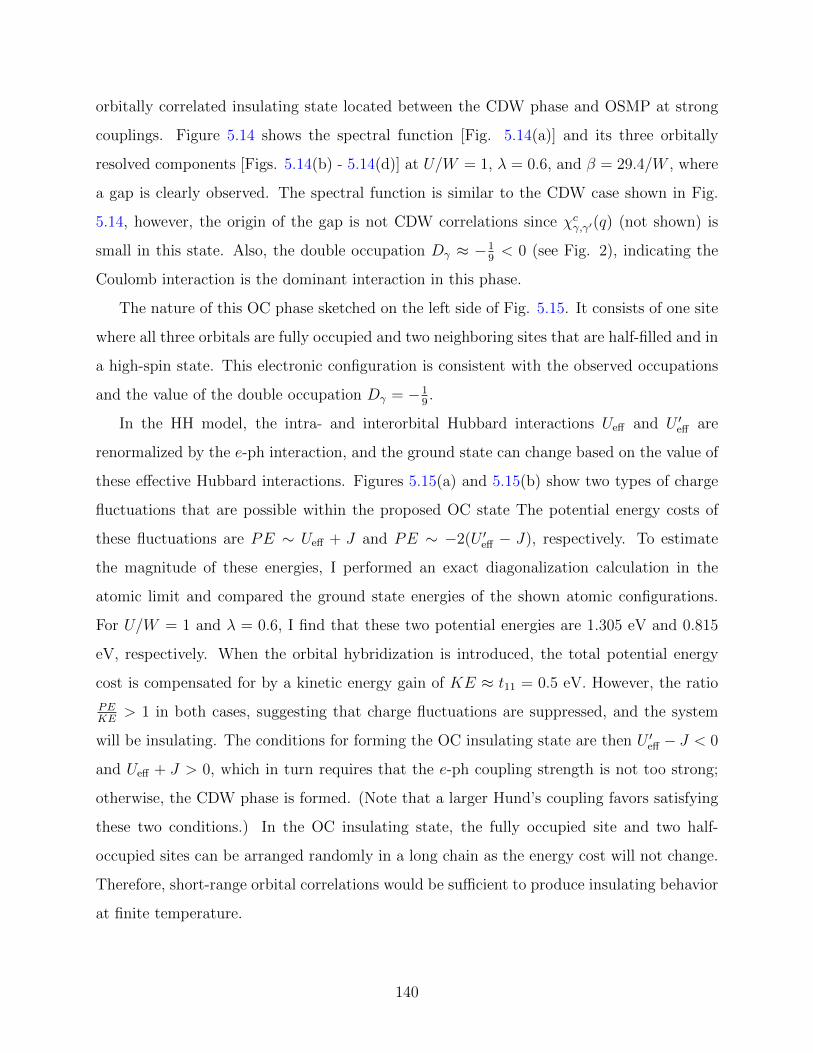
orbitally correlated insulating state located between the CDW phase and OSMP at strong

couplings. Figure 5.14 shows the spectral function [Fig. 5.14(a)] and its three orbitally

resolved components [Figs. 5.14(b) - 5.14(d)] at U/W = 1, λ = 0.6, and β = 29.4/W , where

a gap is clearly observed. The spectral function is similar to the CDW case shown in Fig.

5.14, however, the origin of the gap is not CDW correlations since χcγ,γ′(q) (not shown) is

small in this state. Also, the double occupation Dγ ≈ −19< 0 (see Fig. 2), indicating the

Coulomb interaction is the dominant interaction in this phase.

The nature of this OC phase sketched on the left side of Fig. 5.15. It consists of one site

where all three orbitals are fully occupied and two neighboring sites that are half-filled and in

a high-spin state. This electronic configuration is consistent with the observed occupations

and the value of the double occupation Dγ = −19.

In the HH model, the intra- and interorbital Hubbard interactions Ueff and U ′eff are

renormalized by the e-ph interaction, and the ground state can change based on the value of

these effective Hubbard interactions. Figures 5.15(a) and 5.15(b) show two types of charge

fluctuations that are possible within the proposed OC state The potential energy costs of

these fluctuations are PE ∼ Ueff + J and PE ∼ −2(U ′eff − J), respectively. To estimate

the magnitude of these energies, I performed an exact diagonalization calculation in the

atomic limit and compared the ground state energies of the shown atomic configurations.

For U/W = 1 and λ = 0.6, I find that these two potential energies are 1.305 eV and 0.815

eV, respectively. When the orbital hybridization is introduced, the total potential energy

cost is compensated for by a kinetic energy gain of KE ≈ t11 = 0.5 eV. However, the ratio

PEKE

> 1 in both cases, suggesting that charge fluctuations are suppressed, and the system

will be insulating. The conditions for forming the OC insulating state are then U ′eff − J < 0

and Ueff + J > 0, which in turn requires that the e-ph coupling strength is not too strong;

otherwise, the CDW phase is formed. (Note that a larger Hund’s coupling favors satisfying

these two conditions.) In the OC insulating state, the fully occupied site and two half-

occupied sites can be arranged randomly in a long chain as the energy cost will not change.

Therefore, short-range orbital correlations would be sufficient to produce insulating behavior

at finite temperature.

140

Figure 5.14: (color online) Spectral functions for U/W = 1 and λ = 0.6. Panels (b), (c),and (d) are the orbitals 1, 2, and 3 components of the spectral function in (a). The inversetemperature is β = 29.4/W . The white dot line is the Fermi surface.

141

Figure 5.15: (color online) Cartoon sketch of the relevant charge fluctuation processesleading to the orbital ordered insulating state when U/W = 1 and λ = 0.6.

142

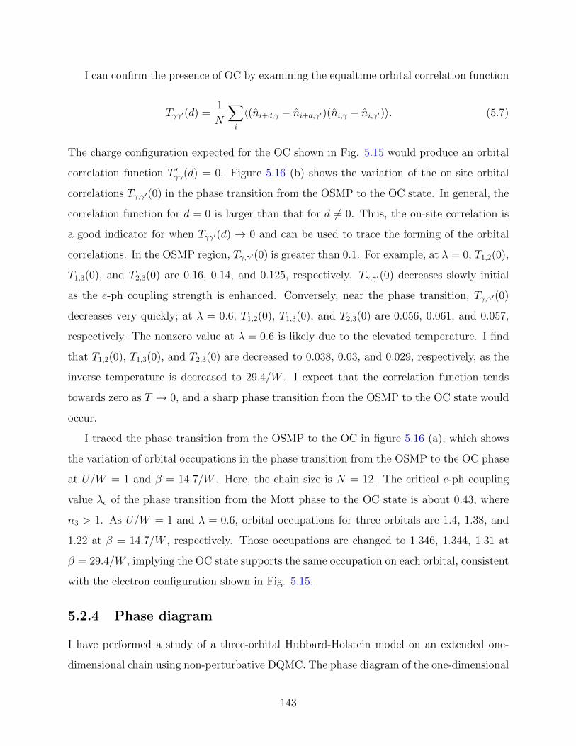
I can confirm the presence of OC by examining the equaltime orbital correlation function

Tγγ′(d) =1

N

∑i

〈(ni+d,γ − ni+d,γ′)(ni,γ − ni,γ′)〉. (5.7)

The charge configuration expected for the OC shown in Fig. 5.15 would produce an orbital

correlation function T ′γγ(d) = 0. Figure 5.16 (b) shows the variation of the on-site orbital

correlations Tγ,γ′(0) in the phase transition from the OSMP to the OC state. In general, the

correlation function for d = 0 is larger than that for d 6= 0. Thus, the on-site correlation is

a good indicator for when Tγγ′(d) → 0 and can be used to trace the forming of the orbital

correlations. In the OSMP region, Tγ,γ′(0) is greater than 0.1. For example, at λ = 0, T1,2(0),

T1,3(0), and T2,3(0) are 0.16, 0.14, and 0.125, respectively. Tγ,γ′(0) decreases slowly initial

as the e-ph coupling strength is enhanced. Conversely, near the phase transition, Tγ,γ′(0)

decreases very quickly; at λ = 0.6, T1,2(0), T1,3(0), and T2,3(0) are 0.056, 0.061, and 0.057,

respectively. The nonzero value at λ = 0.6 is likely due to the elevated temperature. I find

that T1,2(0), T1,3(0), and T2,3(0) are decreased to 0.038, 0.03, and 0.029, respectively, as the

inverse temperature is decreased to 29.4/W . I expect that the correlation function tends

towards zero as T → 0, and a sharp phase transition from the OSMP to the OC state would

occur.

I traced the phase transition from the OSMP to the OC in figure 5.16 (a), which shows

the variation of orbital occupations in the phase transition from the OSMP to the OC phase

at U/W = 1 and β = 14.7/W . Here, the chain size is N = 12. The critical e-ph coupling

value λc of the phase transition from the Mott phase to the OC state is about 0.43, where

n3 > 1. As U/W = 1 and λ = 0.6, orbital occupations for three orbitals are 1.4, 1.38, and

1.22 at β = 14.7/W , respectively. Those occupations are changed to 1.346, 1.344, 1.31 at

β = 29.4/W , implying the OC state supports the same occupation on each orbital, consistent

with the electron configuration shown in Fig. 5.15.

5.2.4 Phase diagram

I have performed a study of a three-orbital Hubbard-Holstein model on an extended one-

dimensional chain using non-perturbative DQMC. The phase diagram of the one-dimensional

143

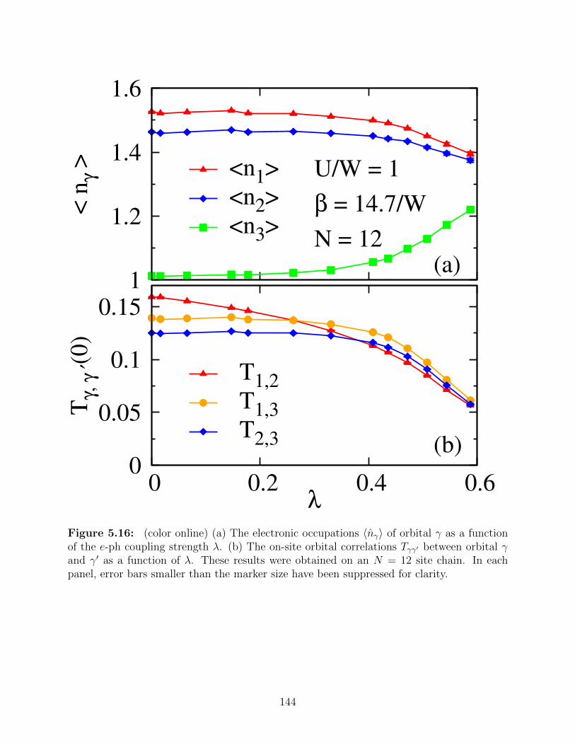
1

1.2

1.4

1.6

0 0.2 0.4 0.6

< n

γ > U/W = 1

β = 14.7/W

N = 12(a)

<n1>

<n2>

<n3>

0

0.05

0.1

0.15

0 0.2 0.4 0.6

Tγ,

γ ′(0

)

λ

(b)

T1,2

T1,3

T2,3

Figure 5.16: (color online) (a) The electronic occupations 〈nγ〉 of orbital γ as a functionof the e-ph coupling strength λ. (b) The on-site orbital correlations Tγγ′ between orbital γand γ′ as a function of λ. These results were obtained on an N = 12 site chain. In eachpanel, error bars smaller than the marker size have been suppressed for clarity.

144

model for β = 14.7/W and n = 4, shown in Fig. 5.17, shares many similarities to the

one found for an infinite-dimensional degenerate two-orbital HH model with inequivalent

bandwidths [149], containing a metallic phase (M), a CDW phase, and an OSMP. The

metallic phase is most prominent in small values of U and λ but penetrates into the region

of intermediate interaction strengths separating the CDW and OSMP when U/W ∼ 2λ.

The critical e-ph coupling needed for the CDW phase transition at U = 0 in the model is

λc ∼ 0.15. The nonzero value of λc is consistent with results for the single band Holstein

model [96, 90].

At strong couplings, I found evidence for an orbital correlation state in the phase diagram,

which was not found in the previous DMFT study. I argue that this difference stems from

the filling used in the model (〈n〉 = 43

here versus 〈n〉 = 1 in Ref. [149]) and the use of

an extended cluster here [148]. The OC state resides between the CDW phase and OSMP

and tends to extend to large Hubbard U . This region of the phase diagram is the same one

where the OSMP disappears, and an anti-ferro-orbital correlation was found in the λ = 0

case [148]. I expect that a phase transition occurs between the anti-ferro-orbital order and

the OC state at U/W = 2. These results show that the phase diagram of multiorbital HH

models can exhibit remarkably rich physics as a function of interaction strengths, doping,

and other parameters.

5.3 Summary

I have studied the interplay between the e-e and e-ph interactions in three- and two-orbital

Hubbard-Holstein model in one- and infinite-dimension, respectively. In both cases, I find a

competition between the onsite e-e and e-ph interactions leads to many competing phases.

In the 1D case, the competition occurs between the OSMP and CDW at small coupling,

while this competition occurs between the OSMP and OSPI in the infinite-dimension. I

also find that the Hund’s coupling J has nontrivial effects on the phases driven by the

e-ph interactions. Importantly, these results demonstrate that weak to intermediate e-ph

interaction strengths can have a significant impact on the phase diagram of this model. As

145

λ

U/W

0

0.1

0.2

0.3

0.4

0.5

0 0.2 0.4 0.6 0.8 1

CDW

M OSMP

OC

Figure 5.17: (color online) The phase diagram of the three-orbital Hubbard-Holsteinmodel for β = 14.7/W and n = 4. The different phases are labeled as follows: metal(M), charge-density-wave order (CDW), orbital selective Mott phase (OSMP), and orbitalcorrelation(OC).

146

such, one cannot rule out an important role for phonons a priori in multi-orbital systems,

when multiple electronic interactions are already competing with one another.

In the past, the e-ph interaction has not been widely studied in the FeSCs in that an

early ab initio calculation shows this interaction strength λ in the FeSCs is too small and

only about 0.21 [26]. However, I find the electronic intrinsic characteristics could have a

significant change under such a small e-ph coupling in both my one- and infinite-dimension

models. These results suggest that one needs to be cautious of the e-ph interaction when

studying FeSCs.

I close with a short note and some speculation. Ref. [241] has also used the term

OSPI in the context of a two-orbital dimer model, where superexchange is stronger between

a particular subset of orbitals, creating a preferential dimerization. An entirely different

mechanism drives the OSPI, where I start from a metallic state and obtain the OSPI through

the e-ph interaction. To the best of my the knowledge, this is the first time that theoretical

calculations have produced such a mechanism. As with OSMP, the OSPI, in this case,

is induced by the different bandwidths for the two orbitals. Finally, although the OSPI

discovered here was derived from a Holstein coupling, I believe bond-stretching phonons

that modulate interatomic hopping integrals could induce a similar phenomenon. In such

cases, these interactions could have a significant impact on nematic phases observed in some

FeSCs [244, 42].

147

Chapter 6

Three-orbital Su-Schrieffer-Heeger

model in two dimensions

6.1 Introduction

Model Hamiltonians have played a vital role in shaping our understanding of e-ph interactions

in materials. These models can be broadly divided into two categories based on whether the

e-ph coupling is diagonal or off-diagonal in the orbital space. Diagonal e-ph interactions

(e.g., in the Holstein [100] or Frohlich [75] models) couple the atomic displacements directly

to the charge density at each site, modulating the carrier’s potential energy. Conversely, off-

diagonal e-ph couplings (e.g., the Su-Schrieffer-Heeger [SSH] [242] model in one-dimension)

occurs when the atomic motion modulates the overlap integrals between neighboring atoms,

generating off-diagonal terms in orbital space.

Diagonal e-ph interactions have received the most attention to date and many techniques

have been employed to study their properties [227, 163, 14, 15, 196, 188, 149, 19]. In the

strong coupling limit, these interactions produce polaronic quasiparticles with large effective

masses m∗ [27, 129, 88, 221, 150], which are prone to forming insulating charge-density-wave

phases [37, 27, 210, 19]. Far fewer studies have been carried out for off-diagonal interactions,

and most of these have been restricted to one-dimension (1D) using either approximate

[242, 146, 171, 239] or quantum Monte Carlo methods [234, 97, 46]. Few studies of SSH-type

148

models in two-dimensions (2D) exist [223, 254, 292, 145], and many of these employ the

frozen phonon approximation [223, 145].

The lack of studies addressing off-diagonal e-ph interactions represents a significant gap

in the communities’ knowledge. These interactions are believed to be the dominant e-ph

interactions in many materials, including the organic charge-transfer solids [242, 146, 45]

and many perovskites systems like the rare-earth nickelates [176, 236, 112], and the high

Tc superconducting cuprates [136, 263] and bismuthates [122]. More importantly, recent

studies in the single- and two-particle limit have shown that the physics of off-diagonal

e-ph interactions differs substantially from that of the more commonly studied diagonal

one. For example, strong off-diagonal interactions can produce highly mobile polarons with

light effective masses [239], generate robust phonon-mediated pairing, and even stabilize

and control the location of a type-II Dirac point [186]. It is, therefore, imperative to study

the off-diagonal e-ph interactions in higher dimensions and for arbitrary fillings, as one’s

intuition gained from the standard diagonal models may not serve us well.

In this chapter, I present a combined exact diagonalization (ED) and determinant

quantum Monte Carlo (DQMC) study of a two-dimensional, multi-orbital sp-model defined

on the Lieb lattice (see Fig. 6.1) with off-diagonal SSH-type e-ph interactions. My approach

treats the problem in a numerically exact manner and does not suffer from a Fermion sign

problem in the absence of a Hubbard interaction. Here, I focus on the so-called “negative

charge transfer” regime [73, 207, 122], where the holes preferentially occupy the oxygen

sublattice. This choice is motivated by the fact that this parameter regime is believed to be

relevant to several perovskite systems with off-diagonal e-ph coupling, including the high-Tc

superconducting bismuthates Ba1−xKxBiO3 [73, 207] and the rare-earth nickelates RNiO3

[112, 200, 23]. Since I neglect the Hubbard interaction, my model can be viewed as a 2D

analog of the model describing the bismuthates. At half-filling, corresponding to one hole per

unit cell, I find that the system is an insulator with a distorted structure, where the ligand

O atoms (the p orbitals) have collapsed and expanded about alternating Bi (the s orbitals)

sites. Upon hole doping, the insulating phase is suppressed giving way to a metallic phase

characterized by holes that are locally bound to fluctuating local structural distortions.

My results provide strong support for the polaronic view often adopted when describing

149

the bismuthates [73, 207], as well as the one recently proposed for the related rare-earth

nickelates [236]. Finally, at low temperatures, I find s-wave superconducting tendencies that

form primarily on the oxygen sublattice.

6.2 Model Hamiltonian

I study a three-orbital model defined on a Lieb lattice, as shown in Fig. 6.1(a). The

orbital basis consists of a Bi 6s atom (red circle) and two O 2p orbitals (blue lobes) situated

halfway between each of the Bi atoms. In what follows, I freeze the heavier Bi atoms into

place and restrict lighter O atoms to move along the bond directions. The full Hamiltonian

is H = H0 +Hlat +He−ph, where

H0 = −tsp∑〈r,δ〉,σ

(Pδ s

†r,σpr,δ,σ + h.c.

)+ tpp

∑〈r,δ,δ′〉,σ

Pδ,δ′p†r,δ,σpr,δ′,σ +

∑r,σ

[(εs − µ)nsr,σ + (εp − µ)(npxr,σ + npyr,σ)

],

Hlat =∑r

(P 2r,x

2M+KX2

r +P 2r,y

2M+KY 2

r

)He−ph = αtsp

∑〈r,δ〉,σ

(ur,δs

†r,σpr,δ,σ + h.c.

).

Here, 〈. . . 〉 denotes a sum over nearest neighbor atoms, δ, δ′ = ±x, ±y index the oxygen

atoms surrounding the Bi sites and the operators s†r,σ, and(sr,σ)

and p†r,δ,σ (pr,δ,σ) are the

creation (annihilation) operators for spin σ holes on the Bi 6s and O 2pδ orbitals, respectively.

The unit cells are indexed by r = nxa+nyb, where (nx, ny) ∈ Z, a = (a, 0), b = (0, a) are the

primitive lattice vectors along x- and y-directions, respectively, and a is the Bi-Bi bond length

in the undistorted structure (and also the unit of length). To simplify the notation, I have

introduced the shorthand notation pr,−x,σ = pr−a,x,σ and pr,−y,σ = pr−b,y,σ. The operators

nsr,σ = s†r,σsr,σ and npαr,σ = p†r,α,σpr,α,σ are the number operators for s and pα (α = x, y)

orbitals, respectively; εs and εp are the onsite energies; µ is the chemical potential; tsp and

tpp are the nearest neighbor Bi-O and O-O hopping integrals in the undistorted crystal;

and α is the e-ph coupling constant. The phase factors are Px(y) = −P−x(−y) = 1, and

150

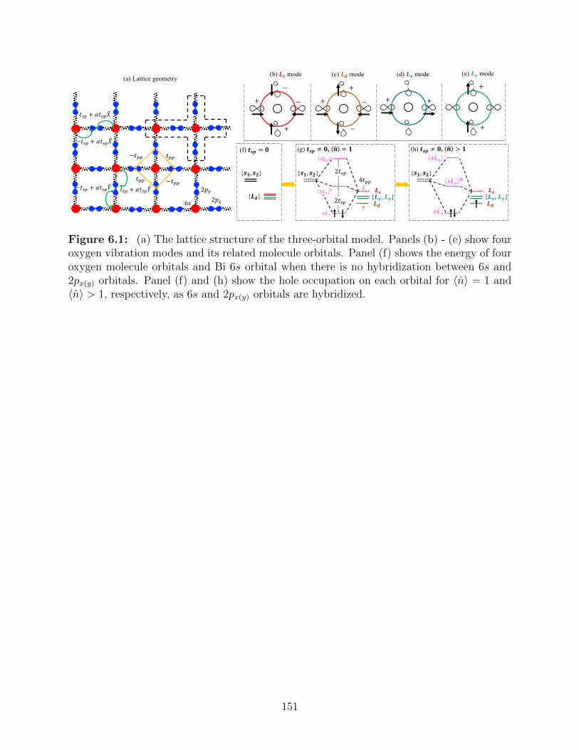
𝑳𝜹

𝒔𝑳𝒔

𝒔𝑳𝒔 ∗

(b) 𝑳𝒔 mode (c) 𝑳𝒅 mode (d) 𝑳𝒙 mode (e) 𝑳𝒚 mode

−

−

+

+

−

+

+

−

++

+

+

𝒔𝟏, 𝒔𝟐

(f) 𝒕𝒔𝒑 = 𝟎 (g) 𝒕𝒔𝒑 ≠ 𝟎, 𝒏3 = 𝟏𝑡55−𝑡55

−𝑡55𝑡55

−𝑡65 + 𝛼𝑡65𝑋9

𝑡65 + 𝛼𝑡65𝑋9

−𝑡65 + 𝛼𝑡65𝑌9 𝑡65 + 𝛼𝑡65𝑌9

2𝑝=

2𝑝>

6𝑠

(a) Lattice geometry

𝑳𝒅𝑳𝒙, 𝑳𝒚𝑳𝒔

2𝑡654𝑡55

𝒔𝑳𝒔 𝟎

𝒔𝟏, 𝒔𝟐

𝒔𝑳𝒔

𝒔𝑳𝒔 ∗

𝒔𝟏, 𝒔𝟐

(h) 𝒕𝒔𝒑 ≠ 𝟎, 𝒏3 > 𝟏

𝑳𝒅𝑳𝒙, 𝑳𝒚𝑳𝒔

𝒔𝑳𝒔 𝟎

2𝑡65

Figure 6.1: (a) The lattice structure of the three-orbital model. Panels (b) - (e) show fouroxygen vibration modes and its related molecule orbitals. Panel (f) shows the energy of fouroxygen molecule orbitals and Bi 6s orbital when there is no hybridization between 6s and2px(y) orbitals. Panel (f) and (h) show the hole occupation on each orbital for 〈n〉 = 1 and〈n〉 > 1, respectively, as 6s and 2px(y) orbitals are hybridized.

151

P±x,±y = P±y,±x = −P±x,∓y = −P∓y,±x = 1. The motion of the lattice is described by the

atomic displacement (momentum) operators Xr,α (Pr,α). M is the oxygen mass and K is

the coefficient of elasticity between each Bi and O atom, and each O atom is linked by two

springs to the neighboring Bi atoms. Thus, the bare phonon frequency is Ω =√

2K/M .

Finally, the displacement of the O atoms modulate the hopping integral as tsp(1 + αur,δ),

where I have introduced shorthand for the displacement operators ur,x = Xr, ur,−x = Xr−a,

ur,y = Yr, and ur,−y = Yr−b.

Throughout, I adopt parameters motivated by a recent DFT study of BaBiO3 [122] with

tsp = 2.08, tpp = 0.056, εs = 6.42, and εp = 2.42 (all in units of eV). As mentioned, these

parameters place us in the negative charge transfer regime, where holes primarily reside on

the O sublattice. For example, at half filling 〈n〉 = 1, I find 〈∑

α,σ npαr,σ〉 = 0.685 in the

absence of the e-ph coupling. The oxygen holes reside in a molecular orbital defined by the

A1g combination of the the ligand oxygen orbitals surrounding the Bi atom (see below) [122].

Finally, I adopt the e-ph coupling strength α = 4a−1.

6.3 A molecular orbital viewpoint

Before I proceed to the DQMC simulations of the model, I present a simplified molecular

orbital analysis of a Bi2O4 cluster, which provides a more transparent view of the physics. I

first expand the simple square unit cell to allow for two distinct Bi 6s orbitals and four O 2p

orbitals, as indicated by the black dashed frame in Fig. 6.1(a). This expanded cell defines

the cluster after I apply periodic boundary conditions. The two Bi 6s orbitals as denoted as

s1 and s2. Next, I transform the four ligand oxygen orbitals into a molecular orbital basis

using

Lr,s,σ =1

2(pr,x,σ + pr,y,σ − pr,−x,σ − pr,−y,σ)

Lr,d,σ =1

2(pr,x,σ − pr,y,σ − pr,−x,σ + pr,−y,σ)

Lr,x,σ =1√2

(pr,x,σ + pr,−x,σ)

Lr,y,σ =1√2

(pr,y,σ + pr,−y,σ).

152

Similarily, I can introduce new phonon operators

xr,Ls =1

2(ur,x + ur,y − ur,−x − ur,−y)

xr,Ld =1

2(ur,x + ur,y − ur,−x − ur,−y)

xr,Lx =1√2

(ur,x + ur,−x)

xr,Ly =1√2

(ur,y + ur,−y),

with an analogous definitions for the momentum operators. Figs. 6.1(b)-6.1(e) sketch the

phases factors of the ligand 2pδ orbitals using ± signs, and the displacement patterns of the

new eigenmodes are indicated by the black arrows. Note that in this representation, the

dimerized structure that forms in the insulating state of the 3D bismuthates and nickelates

corresponds to a coherent state of the optical xr,Ls phonon modes. The xr,Lx and xr,Ly modes

form the basis for the acoustic phonon branches.

After introducing the new basis, the Hamiltonian HM for the Bi2O4 cluster is

HM0 = −2tsp

∑σ

(s†1,σLs,σ − s

†2,σLs,σ + h.c.

)+

(εs − µ)∑σ

(ns1σ + ns2σ ) + (εp − µ)∑

σ,α=x,y

nLασ

+(εp + 2tpp)∑σ

nLsσ + (εp − 2tpp)∑σ

nLdσ

HMlat =

∑γ

(1

2Mp2Lγ +Kx2

Lγ

)HMe−ph = αtsp

∑γ,σ

xLγ

(s†1,σLγ,σ + s†2,σLγ,σ + h.c.

).

Here, the sums on γ are taken over γ = s, d, x, y.

Several insights into the problem at hand can be gleamed from this cluster model. In

the atomic limit (tsp = 0 and tpp = 0) and in the negative charge transfer regime (εp < εs,

in hole language), the four molecular orbitals are degenerate, as shown in Fig. 6.1(f). This

degeneracy is lifted when the atomic overlaps are reintroduced. A nonzero tpp raises (lowers)

the onsite energy of the Ls (Ld) molecular orbital, while a nonzero tsp hybridizes the two Bi

153

s orbitals with the Ls molecular orbital to form new bonding (sLs), nonbonding (sLS)0, and

antibonding (sLs)∗ states. Here, the bonding state’s energy is lowered by 2tsp relative to the

atomic energies, such that the two holes at half filling completely fill this state, as shown in

Fig. 6.1(g). This ground state charge distribution is analogous to the one inferred for 3D

bismuthates in ab initio calculations [73] and ARPES measurements [207].

The impact of the e-ph coupling is also evident from this form of the Hamiltonian; holes

occupying the Lγ molecular orbital couple directly to the phonon eigenmode with the same

symmetry. As such, the holes in the bonding (sLs) state will excite the breathing motion of

the surrounding oxygen atoms. In an extensive system, this coupling can lead to a coherent

state of xLs modes, and a static breathing distortion of the lattice. In this case, a spontaneous

symmetry breaking occurs that selects one of the Bi sites as the center of the compressed

plaquette. From this analysis, it is also clear that additional doped holes will generally enter

the Ld and Lx,y orbitals, where they will excite the other phonon modes. Since the total

displacement of the oxygen atoms is determined by the sum of the individual modes, the

breathing distortion will begin to relax as the other phonon modes are excited. This is the

fundamental mechanism behind the weakening of the static breathing distortion observed in

the doped bismuthates.

To confirm this physical picture, I diagonalized the Hamiltonian HM on a Bi2O4 cluster

and evaluated several observables in the grand canonical ensemble where β = 14.56/tsp,

Ω = tsp, and µ was adjusted to set the particle number. When diagonalizing the model,

I included up to Nph = 5 quanta for each phonon mode, which was sufficient to obtain

converged results for my choice of parameters.

Figure 6.2 summarizes the results of the ED calculations. Panel 6.2(a) and 6.2(b) show

the evolution of the hole density 〈nγ〉 on each molecular orbital, and the fluctuation in the

atomic displacement δ(xγ) = 〈x2γ〉 − 〈xγ〉2, respectively, for each phonon mode as a function

of the total hole occupation of the cluster. At half-filling, the holes occupy the Ls orbital

(the missing weight is on the Bi sites and is not shown for clarity) and no holes occupy the

Ld, Lx, and Ld orbitals. At the same time, the displacement of the xLs mode fluctuates

significantly, while the xLd , xLx , and xLy modes all have fluctuations consistent with zero

point motion, indicating that they are in their ground state.

154

0

0.5

1

1.5<

nγ >

(a)

<nLs>

<nLd>

<nLx>

<nLy>

0.01

0.02

0.03

δ(x

γ)

(b)

zero point vibration

xpx (ypy

)

xLs

xLd

xLx

xLy

0

0.1

0.2

2 2.2 2.4 2.6 2.8 3

<B

γB

γ>

<n>

(c)

Ls

Ld

Lx

Ly

0

0.2

0.4

0.6

2 2.2 2.4 2.6 2.8 3

(bi)

po

laro

n n

um

ber

<n>

(d)

polaron

bipolaron

Figure 6.2: Exact diagonalization results for the Bi2O4 cluster as a function of the totalfilling and at a temperature of β = 14.56/tsp. (a) The hole density on each molecule orbitalas a function of doping. The missing hole weight is located equally on the Bi orbitals and isnot shown. (b) The average fluctuation of the atomic displacement associated with each ofthe four eigenmodes shown in Fig. 1. (c) The average of phonon quanta in the cluster. (d)The expectation value of the polaron and bipolaron operator (see the main text).

155

Upon increasing total hole number, 〈nLs〉 does not change while the occupation on the

other molecular orbitals increases linearly, as expected based on the level diagram shown in

Fig. 6.1(h). In this case, the Ld orbital has a larger hole occupation due to the finite value

of tpp. At the same time, δ(xLd), δ(xLx), and δ(xLd) also increase linearly. The fluctuations

of the four phonon modes are comparable for hole doping 〈n〉 = 2.4− 2.6. The excitation of

xLd , xLx , and xLy phonon modes could also be observed by the phonon number 〈B†γBγ〉 of

each mode, which is shown in Fig. 6.2(c). In the hole doping region 〈n〉 = 2.4 − 2.6, I find

that 〈B†LdBLd〉, 〈B†LxBLx

〉, and 〈B†LyBLy〉 are larger than 〈B†LsBLs

〉, indicating the excitation

of xLd , xLx , and xLy phonons is more prominent than that of xLs phonon. Hence, at this

level of doping, I expect that the dimerized structure would be completely washed out by

the sum of the phonon fluctuations.

To test for the presence of polaron-like objects, I also computed the expectation value of

〈P 〉 = 〈(ns1 + nLs)xLs − (ns2 + nLs)xLs〉

〈BP 〉 = 〈(ns1↑ + nLs↑ )(ns1↓ + nLs↓ )xLs − (ns2↑ + nLs↑ )× (ns2↓ + nLs↓ )xLs〉.

These two quantities represent the number of polaron and bipolaron, respectively, which are

shown in Fig. 6.2(d). With increasing hole dopng, both 〈P 〉 and 〈BP 〉 decrease, implying

that the breathing distortion is suppressed. Throughout whole doping region, I find both

〈P 〉 and 〈BP 〉 are larger than zero, indicating polarons and bipolarons always exist on the

cluster.

6.4 DQMC simulations of an extended lattice

The molecular orbital picture presented in the previous section provides an intuitive way of

understanding the physics of the model. With this in mind, I now turn to detailed DQMC

simulations for the model, defined on an extended cluster withN = 4×4 Bi atoms (48 orbitals

in total) and with Ω =√

2tsp. Here, I am restricted to larger values of the phonon energy

by the long autocorrelation times that develop in DQMC simulations with smaller values of

Ω. All of the remaining parameters are identical to those used in the previous section. With

these values, the DQMC calculations give 〈X〉 = 〈Y 〉 = 0 and 〈X2〉 = 〈Y 2〉 = 0.57(a/4)2 at

156

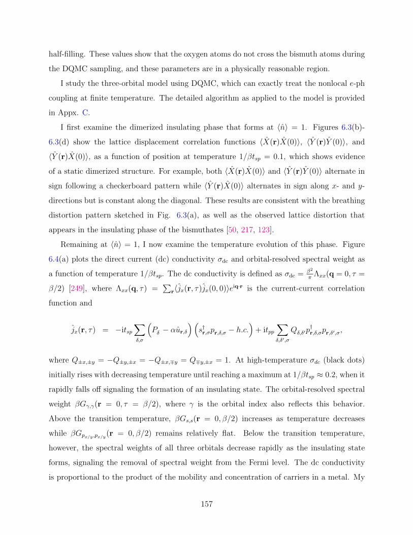
half-filling. These values show that the oxygen atoms do not cross the bismuth atoms during

the DQMC sampling, and these parameters are in a physically reasonable region.

I study the three-orbital model using DQMC, which can exactly treat the nonlocal e-ph

coupling at finite temperature. The detailed algorithm as applied to the model is provided

in Appx. C.

I first examine the dimerized insulating phase that forms at 〈n〉 = 1. Figures 6.3(b)-

6.3(d) show the lattice displacement correlation functions 〈X(r)X(0)〉, 〈Y (r)Y (0)〉, and

〈Y (r)X(0)〉, as a function of position at temperature 1/βtsp = 0.1, which shows evidence

of a static dimerized structure. For example, both 〈X(r)X(0)〉 and 〈Y (r)Y (0)〉 alternate in

sign following a checkerboard pattern while 〈Y (r)X(0)〉 alternates in sign along x- and y-

directions but is constant along the diagonal. These results are consistent with the breathing

distortion pattern sketched in Fig. 6.3(a), as well as the observed lattice distortion that

appears in the insulating phase of the bismuthates [50, 217, 123].

Remaining at 〈n〉 = 1, I now examine the temperature evolution of this phase. Figure

6.4(a) plots the direct current (dc) conductivity σdc and orbital-resolved spectral weight as

a function of temperature 1/βtsp. The dc conductivity is defined as σdc = β2

πΛxx(q = 0, τ =

β/2) [249], where Λxx(q, τ) =∑

r〈jx(r, τ)jx(0, 0)〉eiq·r is the current-current correlation

function and

jx(r, τ) = −itsp∑δ,σ

(Pδ − αur,δ

)(s†r,σpr,δ,σ − h.c.

)+ itpp

∑δ,δ′,σ

Qδ,δ′p†r,δ,σpr,δ′,σ,

where Q±x,±y = −Q±y,±x = −Q±x,∓y = Q∓y,±x = 1. At high-temperature σdc (black dots)

initially rises with decreasing temperature until reaching a maximum at 1/βtsp ≈ 0.2, when it

rapidly falls off signaling the formation of an insulating state. The orbital-resolved spectral

weight βGγ,γ(r = 0, τ = β/2), where γ is the orbital index also reflects this behavior.

Above the transition temperature, βGs,s(r = 0, β/2) increases as temperature decreases

while βGpx/y ,px/y(r = 0, β/2) remains relatively flat. Below the transition temperature,

however, the spectral weights of all three orbitals decrease rapidly as the insulating state

forms, signaling the removal of spectral weight from the Fermi level. The dc conductivity

is proportional to the product of the mobility and concentration of carriers in a metal. My

157

(a) s px (p

y)

0 1 2 3

rx (a)

0

1

2

3

r y (

a)

(b) < X(r)X(0) >

-0.01

-0.005

0

0.005

0.01

0 1 2 3

rx (a)

0

1

2

3

r y (

a)

(c) < Y (r)Y (0) >

(0,0) (3,0) (3,3) (0,0)

r (a)

-0.015

-0.01

-0.005

0

0.005

0.01

0.015

<Y(r)X

(0)>

(d)

Figure 6.3: (a) A sketch of dimerized geometry. The red and blue dots indicate the s andpx,y orbitals, respectively, while the black arrow indicate the displacement pattern of eachoxygen atom in the dimerized structure. Panels (b) and (c) plot the lattice displacementcorrelation functions 〈X(r)X(0)〉 and 〈Y (r)Y (0)〉 as a function of distance r = nxa + nyb,respectively. Here, a and b are the primitive vectors along x- and y-directions, respectively.Panel (d) plots the real-space displacement correlation function 〈Y (r)X(0)〉 indicating thetwo-sublattice structure of the dimerized state. The distance between two nearest Bi atomin the undistorted square structure is a.

158

0

0.3

(0,0) (3,0) (3,3) (0,0)

<n

s (r)n

s (0)>

r (a)

0

0.1

0.2

0.3

0

0.2

0.4

0.6

0.8β

G(r

=0

,τ=

β/2

)

σd

c

(a)

<n>=1

s orb.

px orb.

py orb.

0

10

20

30

0 0.1 0.2 0.3

χC

DW

(π,π

)

1/(βtsp)

(b)

Figure 6.4: (a) The temperature dependence of the spectral weight at the Fermi levelβG(r = 0, τ = β/2) and the direct current (dc) conductivity σdc. (b) The temperaturedependence of the charge-density-wave susceptibility χCDW(π, π). In both panels, the averagefilling is 〈n〉 = 1 corresponding to the “half-filled” case with one hole per unit cell. Errorbars smaller than the marker size have been suppressed for clarity.

159

results show that changes in σdc are correlated with the changes in the concentration of free

carriers.

The formation of charge order in the insulating phase can also be observed in the

charge susceptibility χCγ,γ(q) = 1

N

∫ β0dτ〈nq,γ(τ)nq,γ(0)〉. Here, q is the momentum, τ is

the imaginary time, nq,γ =∑

i,σ eiq·rinri,γ,σ, and ri is the lattice vector. Figure 6.4(b) plots

the temperature evolution of χCγ,γ(q) at q = (π, π), corresponding to the real space ordering

inferred from Fig. 6.3. Below 1/βtps = 0.2, the charge correlations rapidly increase on the s

orbital, while there is little change in the signal on the p orbitals.

The behavior observed in Fig. 6.4 implies that the average density on the O sublattice

remains uniform above and below the metal-to-insulator transition (MIT) while a density

modulation forms on the Bi sites. This view is confirmed in the inset of Fig. 6.4(b), which

plots the equal time Bi-Bi charge density correlation along the high symmetry directions of

the cluster, where a clear (π, π)-ordering is observed. The fact that the charge order signal

appears in the Bi orbital component can be understood once one recognizes that all of the

oxygen orbitals in the system are equivalent, even in the insulating dimerized structure. In

this case, the effect of the breathing distortion is to increase the hybridization between the

Ls orbital and one of the Bi s orbitals at the expense of the other. The two holes are then

shared between the Ls and compressed Bi s orbitals, while no hole occupies the s orbital of

the expanded Bi site, thus accouting for the Bi charge density modulation.

Next, I study effects of hole doping on the MIT at fixed temperature βtsp = 0.1. Figure

6.5(a) plots σdc as a function of filling, where it increases upon hole doping until saturating

at 〈n〉 ≈ 1.4, indicating metallic behavior. I also find evidence for the formation of mobile

polarons in this region, where holes are bound to local breathing distortions of the oxygen

sublattice. This behavior can be seen by examinng the polaron operator p(r) = Xr,Ls(nsr +

nLsr ). The composite operator p(r) measures the presence of a local breathing distortion

centered at site r in combination with holes in the (sLs) orbitals associated with that site.

Figure 6.5(b) plots the doping evolution of the number of polarons given by 1N

∑r〈p(r)〉.

The polaron number is relatively constant in the insulating phase, and monotonically

decreasing in the metallic phase but still nonzero, indicating that a finite number of polarons

are present in the system at all dopings, consistent with the previous conclusion obtained

160

(c) 𝑛" = 1 (d) 𝑛" = 1.38

(e) 𝑛" = 1.44 (f) 𝑛" = 1.59

-2

-1

0

1

2

-2

-1

0

1

2-2 -1 0 1 2 -2 -1 0 1 2

Staggered polaron correlation

-2 -1 0 1 2 -2 -1 0 1 2

-2

-1

0

1

2

-2

-1

0

1

2

(g) 𝑛" = 1 (h) 𝑛" = 1.44

(i) 𝑛" = 1.59 (j) 𝑛" = 1.77

Staggered bipolaron correlation×10./

(a)

(b)

0

0.2

0.4

0.6

0.8

1

σd

c

0

0.2

1 1.2 1.4 1.6 1.8

(bi)

pola

ron n

um

ber

<n>

polaronbipolaron

0.02

0

0.07

0

0.02

-0.01

0.05

0.08

0.06

-0.01

0.06

0.09

0.41

0.09

0.06

-0.01

0.06

0.08

0.05

-0.01

0.02

0

0.07

0

0.02

+-0.07

+-0.04

+-0.06

+-0.04

+-0.07

+-0.04

+-0.04

+-0.03

+-0.04

+-0.04

+-0.04

+-0.02

+-0.06

+-0.02

+-0.04

+-0.04

+-0.04

+-0.03

+-0.04

+-0.04

+-0.07

+-0.04

+-0.06

+-0.04

+-0.07

0.28

0.12

0.31

0.12

0.28

0.12

0.29

0.14

0.29

0.12

0.29

0.14

0.52

0.14

0.29

0.12

0.29

0.14

0.29

0.12

0.28

0.12

0.31

0.12

0.28

+-0.1

+-0.04

+-0.1

+-0.04

+-0.1

+-0.04

+-0.08

+-0.03

+-0.08

+-0.04

+-0.09

+-0.03

+-0.09

+-0.03

+-0.09

+-0.04

+-0.08

+-0.03

+-0.08

+-0.04

+-0.1

+-0.04

+-0.1

+-0.04

+-0.1

-0.02

-0.02

0.04

-0.02

-0.02

-0.03

0.04

0.09

0.03

-0.03

0.04

0.08

0.41

0.08

0.04

-0.03

0.03

0.09

0.04

-0.03

-0.02

-0.02

0.04

-0.02

-0.02

+-0.07

+-0.04

+-0.06

+-0.04

+-0.07

+-0.04

+-0.03

+-0.02

+-0.04

+-0.04

+-0.05

+-0.02

+-0.07

+-0.02

+-0.05

+-0.04

+-0.04

+-0.02

+-0.03

+-0.04

+-0.07

+-0.04

+-0.06

+-0.04

+-0.07

-0.03

-0.02

0.01

-0.02

-0.03

-0.03

0

0.08

0

-0.03

0.02

0.08

0.4

0.08

0.02

-0.03

0

0.08

0

-0.03

-0.03

-0.02

0.01

-0.02

-0.03

+-0.06

+-0.04

+-0.05

+-0.04

+-0.06

+-0.04

+-0.02

+-0.03

+-0.02

+-0.04

+-0.05

+-0.02

+-0.06

+-0.02

+-0.05

+-0.04

+-0.02

+-0.03

+-0.02

+-0.04

+-0.06

+-0.04

+-0.05

+-0.04

+-0.06

-0.03

-0.02

0.01

-0.02

-0.03

-0.03

0

0.08

0

-0.03

0.02

0.08

0.4

0.08

0.02

-0.03

0

0.08

0

-0.03

-0.03

-0.02

0.01

-0.02

-0.03

+-0.06

+-0.04

+-0.05

+-0.04

+-0.06

+-0.04

+-0.02

+-0.03

+-0.02

+-0.04

+-0.05

+-0.02

+-0.06

+-0.02

+-0.05

+-0.04

+-0.02

+-0.03

+-0.02

+-0.04

+-0.06

+-0.04

+-0.05

+-0.04

+-0.06

0.1

0

0.11

0

0.1

0

0.1

0

0.1

0

0.1

0

1.42

0

0.1

0

0.1

0

0.1

0

0.1

0

0.11

0

0.1

+-0.03

+-0

+-0.03

+-0

+-0.03

+-0

+-0.03

+-0

+-0.03

+-0

+-0.03

+-0

+-0.24

+-0

+-0.03

+-0

+-0.03

+-0

+-0.03

+-0

+-0.03

+-0

+-0.03

+-0

+-0.03

0.01

-0.02

0.02

-0.02

0.01

-0.02

0.02

0

0.02

-0.02

0.02

0

1

0

0.02

-0.02

0.02

0

0.02

-0.02

0.01

-0.02

0.02

-0.02

0.01

+-0.01

+-0.01

+-0.01

+-0.01

+-0.01

+-0.01

+-0.01

+-0

+-0.01

+-0.01

+-0.02

+-0

+-0.17

+-0

+-0.02

+-0.01

+-0.01

+-0

+-0.01

+-0.01

+-0.01

+-0.01

+-0.01

+-0.01

+-0.01

0

-0.01

0.01

-0.01

0

-0.01

0.01

0.01

0.01

-0.01

0.01

0.01

0.96

0.01

0.01

-0.01

0.01

0.01

0.01

-0.01

0

-0.01

0.01

-0.01

0

+-0.01

+-0.01

+-0.01

+-0.01

+-0.01

+-0.01

+-0

+-0.01

+-0

+-0.01

+-0.01

+-0

+-0.16

+-0

+-0.01

+-0.01

+-0

+-0.01

+-0

+-0.01

+-0.01

+-0.01

+-0.01

+-0.01

+-0.01

-0.01

0

0.01

0

-0.01

-0.01

0

0.01

0

-0.01

0

0.01

0.96

0.01

0

-0.01

0

0.01

0

-0.01

-0.01

0

0.01

0

-0.01

+-0.01

+-0.01

+-0.01

+-0.01

+-0.01

+-0.01

+-0.01

+-0.01

+-0.01

+-0.01

+-0.01

+-0.01

+-0.19

+-0.01

+-0.01

+-0.01

+-0.01

+-0.01

+-0.01

+-0.01

+-0.01

+-0.01

+-0.01

+-0.01

+-0.01

Figure 6.5: (a) The dc conductivity as a function of doping. (b) polaron and bipolaronnumber as a function of doping. (c)-(f) Staggered polaron correlation function 〈P (r)〉 and(h)-(j) staggered bipolaron correlation function 〈BP (r)〉 at different doping levels. The red(gray) color indicates values larger (smaller) than zero. The numerical value of the correlationfunction, along with the associated 1σ statistical error are indicated at each point. All resultsare for a temperature 1/(βtsp) = 0.1 and error bars smaller than the marker size have beensuppressed for clarity.

161

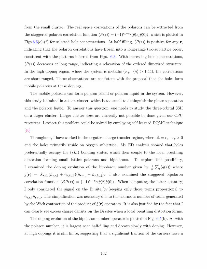
from the small cluster. The real space correlations of the polarons can be extracted from

the staggered polaron correlation function 〈P (r)〉 = (−1)rx+ry〈p(r)p(0)〉, which is plotted in

Figs.6.5(c)-(f) for selected hole concentrations. At half filling, 〈P (r)〉 is positive for any r,

indicating that the polaron correlations have frozen into a long-range two-sublattice order,

consistent with the patterns inferred from Figs. 6.3. With increasing hole concentrations,

〈P (r)〉 decreases at long range, indicating a relaxation of the ordered dimerized structure.

In the high doping region, where the system is metallic (e.g. 〈n〉 > 1.44), the correlations

are short-ranged. These observations are consistent with the proposal that the holes form

mobile polarons at these dopings.

The mobile polarons can form polaron island or polaron liquid in the system. However,

this study is limited in a 4× 4 cluster, which is too small to distinguish the phase separation

and the polaron liquid. To answer this question, one needs to study the three-orbital SSH

on a larger cluster. Larger cluster sizes are currently not possible be done given our CPU

resources. I expect this problem could be solved by employing self-learned DQMC technique

[40].

Throughout, I have worked in the negative charge-transfer regime, where ∆ = εs− εp > 0

and the holes primarily reside on oxygen sublattice. My ED analysis showed that holes

preferentially occupy the (sLs) bonding states, which then couple to the local breathing

distortion forming small lattice polarons and bipolarons. To explore this possibility,

I examined the doping evolution of the bipolaron number given by 1N

∑r〈g(r)〉 where

g(r) = Xr,Ls(nr,s,↑ + nr,Ls,↑)(nr,s,↓ + nr,Ls,↓). I also examined the staggered bipolaron

correlation function 〈BP (r)〉 = (−1)rx+ry〈g(r)g(0)〉. When computing the latter quantity,

I only considered the signal on the Bi site by keeping only those terms proportional to

nr,s,↑nr,s,↓. This simplification was necessary due to the enormous number of terms generated

by the Wick contraction of the product of g(r) operators. It is also justified by the fact that I

can clearly see excess charge density on the Bi sites when a local breathing distortion forms.

The doping evolution of the bipolaron number operator is plotted in Fig. 6.5(b). As with

the polaron number, it is largest near half-filling and decays slowly with doping. However,

at high dopings it is still finite, suggesting that a significant fraction of the carriers have a

162

bipolaron character. The staggered bipolaron correlation function is plotted in Figs. 6.5(g)-

(j). At 〈n〉 = 1, the bipolaron correlations are clear and long-ranged. This result lends to

the interpretation that the insulating phase can be thought of as a static bipolaron lattice.

As the hole concentration is increased, however, I find that the bipolaron correlations are

entirely suppressed at all length scales, while a finite number of bipolarons are present in

the system, as indicated in Fig. 4b. These results support the notion that mobile bipolarons

exist in the metallic phase.

This scenario raises questions regarding possible superconductivity. I therefore computed

the pair field susceptibility χγsc = 1N

∫ β0dτ〈∆γ(τ)∆†γ(0)〉, where ∆s =

∑r sr,↑sr,↓ and ∆pδ =∑

r pr,δ,↑pr,δ,↓. Since χpxsc and χpysc are the same, I use χpsc to denote pairing on the O atoms.

Figure 6.6 plots χγsc as a function of temperature at 〈n〉 = 1.59, and compares it against the

dominant charge correlations at this doping χCss(π, π/2). All three susceptibilities increase

with decreasing temperature, but χpsc dominates below 1/βtsp ≈ 0.04. Extrapolating 1/χsc to

zero (as shown in the inset), yields a Tc ≈ 382 K (1/βtsp ≈ 0.0158). This value is artificially

high, due to the large value of Ω used in the calculations. Nevertheless, these results provide

evidence that the bipolaronic rich metallic phase has a superconducting ground state.

6.5 Discussion and Summary

I have studied off-diagonal e-ph interactions in the 2D three-orbital model on a Lieb

lattice. At half filling, I find a MIT at low temperature, which is accompanied by a lattice

dimerization, consistent with the charge-ordered insulating state observed in the 3D barium

bismuthates. The insulating phase is suppressed upon hole doping, leading to a metallic

phase with evidence of delocalized polaronic carriers. I argue that the relaxation of the

breathing distortions with doping can be understood from the excitation of the other types

of phonon modes when holes are introduced to the unoccupied molecular orbitals in the

material. I again stress that in this picture the breathing distortion relaxes when a significant

number of additional phonon modes are excited by the doped holes entering the unoccupied

molecular orbitals. In other words, the breathing-type optical phonons are still present in

the doped system due to the significant number of holes that remain in the Ls molecular

163

0

0.5

1

1.5

2

0.05 0.1 0.15

χ

1/βtsp

(a)χC(π,π/2)

χssc

χp

sc 0

1

2

0 0.1

1/χ

psc

1/βtsp

1

1.5

2

1.5 1.6 1.7

χp

sc

<n>

(b) 1/βtsp = 0.03

Figure 6.6: (a) The charge-density-wave χCDW(π, 0) and pairing χSC susceptibilities asa function of temperature 1/(βtsp) at 〈n〉 = 1.59. The inset plots 1/χpsc as a function oftemperature 1/(βtsp). The black dashed line is the fitting result. (b) The doping dependenceof χSC at a temperature of 1/(βtsp) = 0.03. Error bars smaller than the marker size havebeen suppressed for clarity.

164

orbital. Overall, my results are consistent with a picture where polarons create fluctuating

local lattice distortions in the metallic phase but freeze into an ordered insulating phase

below the MIT. Moreover, I find an s-wave superconducting state at finite doping, where

the superconducting tendencies form on the oxygen sublattice as the system cools.

Finally, I stress that I have studied the off-diagonal e-ph interaction in a model that

includes multiple orbitals. Previously, it has been proposed that this model can be

downfolded onto an effective single band model with an attractive Hubbard interaction

[217, 209, 168, 116, 281, 107, 22]. Since neither model suffers from a Fermion sign problem,

it would be interesting to contrast the pictures created by these two scenarios to test the

validity of this proposal.

165

Chapter 7

Summary and outlook

Although many studies claim that the fluctuations are essential to the high-TC supercon-

ductors, including the cuprates and iron-based superconductors, there are many lines of

evidence show that the phonon is not negligible as discussed in chapter 1. In general, there

are two types of e-ph couplings used in theoretical models. The first one is the local e-ph

coupling, which links the displacement of an atom to the total charge density in a given

orbital. One typical model for the local e-ph coupling is the Holstein model. To understand

the role of phonons in strongly correlated systems, the Holstein model has been extended

to the Hubbard-Holstein (HH) model, which includes both e-e and e-ph coupling. To date,

the single band HH model has been studied in various dimensions with different fillings

[20, 44, 163, 90, 196, 14, 113, 131]. But the role of phonons in strongly correlated systems

has not been fully understood. For example, the non-linear e-ph coupling, which cannot

be captured by the Holstein model, has not been widely studied, although it is proposed

that the non-linear e-ph coupling could suppress the electron-boson coupling in a cuprate

superconductor [289]. This fact asks us to continuously explore the interplay between the

e-e and e-ph interactions. Moreover, the correlated materials are not always captured by the

single-band model. For example, the iron-based superconductors are multiorbital materials,

which have five d orbitals near the Fermi surface [81]. In this case, one needs to extend the

single-band HH model to a multiorbital HH model.

The second e-ph coupling is the nonlocal e-ph coupling, which links the displacement of

an atom to both its nearest neighbors and itself. The typical model for the nonlocal e-ph

166

coupling is the Su-Schreiff-Heeger model [242]. This model has been extensively studied

in the one-dimension and the single-band case [146, 234, 97, 46]. But many high-TC

superconductors are high-dimensional multiorbital materials. Then to study the role of

the nonlocal e-ph coupling in those high-TC superconductors, such as barium bismuthate

and high-TC cuprates, one needs to build the SSH model in a high-dimension with multiple

orbitals.

In sum, the role of phonons in high-TC superconductors has not been completely

understood to date. In this dissertation, I continue to explore the role of phonons in high-TC

superconductors. My project included three parts: (1) the non-linear e-ph coupling, (2)

the interplay between e-ph and e-e couplings in a multiorbital system, and (3) breathing

phonons in a two-dimensional multiorbital model.

The first part of my research studied the non-linear e-ph coupling in a nonmagnetic

system [147, 148]. It was found that a positive non-linear e-ph interaction could dramatically

suppress the CDW correlations that dominate the linear Holstein model and a negative non-

linear e-ph interaction has an opposite effect. Both the positive and negative non-linear

e-ph interactions have a less pronounced effect for the superconducting correlations. These

effects are attributed to a combined hardening of the phonon mode and weakening of the

effective linear coupling by the positive non-linear terms, or softening of the phonon mode

and enhancing of the effective linear coupling by the negative non-linear terms. I also found

that the electronic and phononic properties of the non-linear Holstein model cannot be

captured by an effective linear Holstein model simultaneously, indicating that one should be

cautions of the strength of the e-ph interaction in pump-probed experiments. In this work,

I didn’t include the e-e interaction. To understand the role of non-linear e-ph interaction in

a correlated materials, where e-e interactions is not negligible, I will study a modified HH

model in the future, which includes both linear and non-linear e-ph coupling.

The second part of my research studies the interplay between the linear e-ph and e-

e couplings in a multiorbital system [148]. In the single band HH model, the interplay

between the e-e and e-ph interactions leads a competition between the CDW phase and

MI phase [14, 196, 113]. But in the multiorbital Hubbard-Holstein model, the situatution

is more complex due to an extra orbital degree of freedom. It was shown that the orbital

167

degree of freedom is essential to some new phases discovered in the multiorbital Hubbard

model. One of the new phases is the OSMP, in which some orbitals are Mott insulators and

the other orbitals remain metallic. When the Holstein phonon is included in the multiorbital

Hubbard model, a phase transition from the OSMP phase to the CDW phase could be

found. Moreover, when the ratio between bands is large enough, an OSPI appears. Both

the OSMP and OSPI are the results of the orbital degree of freedom, which is absent in the

single band HH model. In addition, it was found that the e-ph coupling strength for the

phonon dominated phase in the multiorbital system is not necessary very large, indicating

that the phonon in the multiorbital material, such as FeSC, could be more important than

what people expect.

The third part of my research focuses on the breathing phonons in barium bismuthate.

Here, I present a method for modeling the off-diagonal e-ph coupling in a three-orbital model

using DQMC for the first time. The three-orbital SSH model includes Bi 6s and O 2px/y

orbitals, which is a 2D analog of the barium bismuthate high TC superconductors. I find a

metal-insulator transition with decreasing temperature at half filling and identify a dimerized

structure in the insulating phase. At the same time, a charge-density-wave (CDW) appears

on the Bi 6s orbital. With hole doping, the ordered polarons and bipolarons correlations

disappear but the short-range correlations are present, implying that polarons and bipolarons

preform in the metallic phase. At a finite doping, I observe that an s-wave superconducting

fluctuation first appears on oxygen atoms as temperature decreases and becomes an ordered

state at low temperature.

These are three studies I have done in this dissertation, but there are many more questions

needed to be studied in the future. The first one is studying the interorbital scattering

in a multiorbital HH model. In the single band model, phonons and electrons could be

renormalized by intra-orbital scattering. In the multiorbital model, one might expect that

the properties of both phonons and electrons could be modified by the extra scattering,

namely inter-orbital scattering. But it is not clear how the inter-orbital scattering changes

both properties. Comparing the CDW phase transition in the one-, two-, and three-orbital

system can give us a direct clue how the orbital degree of freedoms reshapes both electronic

and phononic properties. The second question concerns studying the phase diagram of the

168

three-orbital Hubbard-SSH model on a two-dimensional layer. This work directly relates to

the cuprates. The thrid question is understanding the interplay between the holstein phonon

and the breathing phonon. In a one dimension, the charge order induced by the holstein

phonon is ”2000” type at a quarter filling, while the charge order induced by the breathing

phonon is ”0110” type [46]. These two charge ordered states will compete with each other

in a model including both the local e-ph and nonlocal e-ph interactions. Studying the phase

diagram of the Holstein-SSH model is helpful to understand microscopic mechanism of quasi-

one-dimensional organic superconductors, such as (DMEDO− TTF)2X, X = ClO4 and BF4

[175, 283, 285, 46, 125].

Throughout this work a number of aspects of e-ph coupling have been examined. The

highlighted jobs are the e-ph coupling in the multiorbital correlated system and the nonlocal

e-ph coupling project. My work first points out that the e-ph coupling strength for the

phonon-mediated phenomenon in a multiorbital system is not necessary large. Previous DFT

studies claim that the e-ph interaction strength in FeSCs is too small to change electronic

properties [26]. My results alert the community to notice even a weak e-ph interaction is

still important in a multiorbital system. The nonlocal e-ph coupling project paves a way to

exactly study the SSH model in a high-dimension using DQMC. This is important since many

nonlocal e-ph coupling problems are solved by classical methods or perturbation techniques

[223, 254, 292, 145]. It is not clear how reliable results obtained from these perturbation

theories are. Here, DQMC can be used to evaluate these perturbation theories. In summary,

my research not only broadens the view of phonons in multiorbital systems but also lays a

foundation for fully understanding the role of phonons in multiorbital systems.

169

Bibliography

170

[1] Adolphs, C. P. J. and Berciu, M. (2013). Going beyond the linear approximation

in describing electron-phonon coupling: relevance for the Holstein model. EPL.,

102(4):47003. 52, 54, 55, 58, 59, 73, 76, 80, 84

[2] Adolphs, C. P. J. and Berciu, M. (2014a). Single-polaron properties for double-well

electron-phonon coupling. Phys. Rev. B, 89(3):035122. 80

[3] Adolphs, C. P. J. and Berciu, M. (2014b). Strongly bound yet light bipolarons for

double-well electron-phonon coupling. Phys. Rev. B, 90(8):085149. 52

[4] Akerlund, O., Forcrand, P. d., Georges, A., and Werner, P. (1999). Dynamical mean field

approximation applied to quantum field theory. Phys. Rev. D, 88(12):125006. 95

[5] Anisimov, V. I., Nekrasov, I. A., Kondakov, D. E., Rice, T. M., and Sigrist, M. (2002).

Orbital-selective Mott-insulator transition in Ca2−xSrxRuO4. Eur. Phys. J. B, 25(2):191.

85, 113

[6] Arsenault, L.-F., Semon, P., and Tremblay, A.-M. S. (2012). Benchmark of a modified

iterated perturbation theory approach on the fcc lattice at strong coupling. Phys. Rev. B,

86(8):085133. 62

[7] Aryanpour, K., Pickett, W. E., and Scalettar, R. T. (2006). Dynamical mean-field study

of the Mott transition in the half-filled Hubbard model on a triangualr lattice. Phys. Rev.

B, 74(8):085117. 14

[8] Awan, A. and Lancashire, R. J. (2016). Crystal field theory. https://chem.libretexts.

org/Core/Inorganic_Chemistry/Crystal_Field_Theory/Crystal_Field_Theory. 8

[9] Bardeen, J., Cooper, L. N., and Schrieffer, J. R. (1957). Theory of superconductivity.

Phys. Rev., 108(5):1175. 1, 52

[10] Barisic, N., Chan, M. K., Li, Y., Yu, G., Zhao, X., Dressel, M., Smontara, A., and

Greven, M. (2013). Universal sheet resistance and revised phase diagram of the cuprate

high-temperature superconductors. PNAS., 110(30):12235. 3

[11] Batlogg, B. (1984). Superconductivity in Ba(Pb,Bi)O3. Physica B, 126(1-3):275. 12

171

https://chem.libretexts.org/Core/Inorganic_Chemistry/Crystal_Field_Theory/Crystal_Field_Theory

https://chem.libretexts.org/Core/Inorganic_Chemistry/Crystal_Field_Theory/Crystal_Field_Theory

[12] Batlogg, B., Cava, R. J., Jayaraman, A., Dover, R. B. v., Kourouklis, G. A., Sunshine,

S., Murphy, D. W., Rupp, L. W., Chen, H. S., White, A., Short, K. T., Mujsce, A. M.,

and Rietman, E. A. (1987). Isotope effect in the high-TC superconductors Ba2YCu3O7

and Ba2EuCu3O7. Phys. Rev. Lett., 58(22):2333. 19

[13] Batlogg, B., Cava, R. J., Rupp, L. W., Mujsce, A. M., Krajewski, J. J., Pemeika, J. P.,

Peck, W. F., Cooper, A. S., and Espinosa, G. P. (1988). Density of states and isotope

effect in BiO superconductors: evidence for nonphonon mechanism. Phys. Rev. Lett.,

61(14):1670. 22

[14] Bauer, J. (2010). Competing interactions and symmetry breaking in the Hubbard-

Holstein model. EPL, 90(2):27002. 114, 117, 148, 166, 167

[15] Bauer, J. and Hewson, A. C. (2010). Competition between antiferromagnetic and charge

order in the Hubbard-Holstein model. Phys. Rev. B, 81(23):235113. 114, 117, 120, 125,

148

[16] Beach, K. S. D. and Assaad, F. F. (2011). Orbital-selective Mott transition and heavy-

fermion behavior in a bilayer Hubbard model for 3He. Phys. Rev. B, 83(4):045103. 86

[17] Bednorz, J. G. and Mueller, K. A. (1986). Possible high TC superconductivity in the

Ba-La-Cu-O system. Zeitschrift fur Physik, 64(2):189–193. 2

[18] Beichi, I. and Sullivan, F. (2000). The metropolis algorithm. Computing in Science and

Engineering, 2(1):65–69. 30

[19] Berciu, M. (2006). Green’s function of a dressed particle. Phys. Rev. Lett., 97:036402.

148

[20] Berger, E., Valasek, P., and Linden, W. v. d. (1995). Two-dimensional Hubbard-Holstein

model. Phys. Rev. B, 52(7):4806. 114, 166

[21] Biermann, S., Medici, L. d., and Georges, A. (2005). Non-fermi-liquid behavior and

double-exchange physics in orbital-selective Mott systems. Phys. Rev. Lett., 95(20):206401.

86

172

[22] Bischofs, I. B., Allen, P. B., Kostur, V. N., and Bhargave, R. (2002). Topological doping

of a three-dimensinal peierls system: Predicted structure of doped BaBiO3. Phys. Rev. B,

66(17):174108. 165

[23] Bisogni, V., Catalano, S., Green, R. J., Gibert, M., Scherwitzl, R., Huang, Y., Strocov,

V. N., Zubko, P., Balandeh, S., Triscone, J.-M., G., S., and Schmitt, T. (2016). Ground-

state oxygen holes and the metalinsulator transition in the negative charge-transfer rare-

earth nickelates. Nature Communications, 7:13017. 149

[24] Blankenbecler, R., Scalapino, D. J., and Sugar, R. L. (1981). Monte carlo calculations

of coupled boson-fermion systems. I. Phys. Rev. D, 24(8):2278–2286. 27, 28

[25] Boeri, L., Calandra, M., Mazin, I. I., Dolgov, O. V., and Mauri, F. (2010). Effects

of magnetism and doping on the electron-phonon coupling in BaFe2As2. Phys. Rev. B,

82(2):020506. 21, 114

[26] Boeri, L., Dolgov, O. V., and Golubov, A. A. (2008). Is LaFeAsO1−xFx an electron-

phonon superconductor? Phys. Rev. Lett., 101(2):026403. 21, 114, 147, 169

[27] Bonca, J., Trugman, S. A., and Batistic, I. (1999). Holstein polaron. Phys. Rev. B,

60:1633–1642. 148

[28] Bouadim, K., Batrouni, G. G., Hebert, F., and Scalettar, R. T. (2008). Magnetic and

transport properties of a coupled Hubbard bilayer with electron and hole doping. Phys.

Rev. B, 77(14):144527. 89

[29] Bouadim, K., Batrouni, G. G., and Scalettar, R. T. (2009). Determinant quantum monte

carlo study of the orbitally selective Mott transition. Phys. Rev. Lett., 102(22):226402. 86

[30] Bourne, L. C., Crommie, M. F., Zettl, A., Loye, H.-C. z., Keller, S. W., Leary, K. L.,

Stacy, A. M., Chang, K. J., Cohen, M. L., and Morris, D. E. (1987). Search for isotope

effect in superconducting Y −Ba− Cu−O. Phys. Rev. Lett., 58(22):2337. 19

[31] Boyce, J. B., Bridges, F. G., Claeson, T., Geballe, T. H., and Remeika, J. M.

(1990). X-ray absorption of BaBiO3 and superconducting BaBi0.25Pb0.75O3. Phys. Rev.

B, 41(10):6306. 9

173

[32] Bryan, R. K. (1990). Maximum entropy analysis of oversampled data problems.

European Biophysics Journal, 18(3):165–174. 48, 49

[33] Capone, M., Castellani, C., and Grilli, M. (2010). Electron-phonon interaction in

strongly correlated systems. Adv. Condens. Matter Phys., 2010(920860):1–18. 114

[34] Caron, J. M., Neilson, J. R., Miller, D. C., Arpino, K. ad Llobet, A., and McQueen,

T. M. (2012). Orbital-selective magnetism in the spin-ladder iron selenides Ba1−xKxFe2Se3.

Phys. Rev. B, 85(18):180405(R). 87

[35] Caron, J. M., Neilson, J. R., Miller, D. C., Llobet, A., and McQueen, T. M. (2011). Iron

displacements and magnetoelastic coupling in the antiferromagnetic spin-ladder compound

BaFe2Se3. Phys. Rev. B, 84(18):180409. 87

[36] Castellani, C., Castro, C. D., Feinberg, D., and Ranninger, J. (1979). New model

hamiltonian for the metal-insulator transition. Phys. Rev. Lett., 43(26):1957. 115, 127

[37] Chakraverty, B. K., Ranninger, J., and Feinberg, D. (1998). Experimental and

theoretical constraints of bipolaronic superconductivity in high Tc materials: An

impossibility. Phys. Rev. Lett., 81:433–436. 148

[38] Chan, C.-K., Werner, P., and Millis, A. J. (2009). Magnetism and orbital ordering in an

interacting three-band model: a dynamical mean-field study. Phys. Rev. B, 80(23):235114.

86, 106

[39] Chang, J., Eremin, I., and Thalmeier, P. (2009). Cooper-pair formation by anharmonic

ratting modes in the β-pyrochlore superconductor KOS2O6. New. J. Phys., 11(5):055068.

84

[40] Chen, C., Xu, X. Y., Liu, J., Batrouni, G., Scalettar, R., and Meng, Z. Y. (2018).

Symmetry enforced self-learning monte carlo method applied to the holstein model.

arXiv:1802.06177. 162

[41] Chi, S., Johnston, S., Levy, G., Grothe, S., Szedlak, R., Lubrook, B., Liang, R., Dosanjh,

P., Burke, S. A., Damascelli, A., Bonn, D. A., Hardy, W. N., and Pennec, Y. (2014). Sign

174

inversion in the superconducting order parameter of LiFeAs inferred from Bogoliubov

quasiparticle interference. Phys. Rev. B, 89(10):104522. 99

[42] Chu, J.-H., Kuo, H.-H., Analytis, J. G., and Fisher, I. R. (2012). Divergent nematic

susceptibility in an iron arsenide superconductor. Science, 337(6095):710. 147

[43] Ciuchi, S. and Fratini, S. (2011). Band dispersion and electronic lifetimes in crystalline

organic semiconductors. Phys. Rev. Lett., 106(16):166403. 52

[44] Clay, R. T. and Hardikar, R. P. (2005). Intermediate phase of the one dimensional

half-filled Hubbard-Holstein model. Phys. Rev. Lett., 95(9):096401. 125, 166

[45] Clay, R. T. and Mazumdar, S. (2018). From charge- and spin-ordering to

superconductivity in the organic charge-transfer solids. 149

[46] Clay, R. T., Ward, A. B., Gomes, N., and Mazumdar, S. (2017). Bond patterns

and charge-order amplitude in quarter-filled charge-transfer solids. Phys. Rev. B,

95(2017):125114. 148, 167, 169

[47] Coh, S., Cohen, M. L., and Louie, S. G. (2015). Large electron-phonon interactions

from FeSe phonons in a monolayer. New J. Phys., 17(7):073027. 21, 114

[48] Coh, S., Cohen, M. L., and Louie, S. G. (2016). Antiferromagnetism enables electron-

phonon coupling in iron-based superconductors. Phys. Rev. B, 94(10):104505. 21, 114

[49] Cooper, S. L., Reznik, D., Kotz, A., Kariow, M. A., Liu, R., Klein, M. V., Lee, W. C.,

Giapintzakis, J., Ginsberg, D. M., Veal, B. W., and Paulikas, A. P. (1993). Optical studies

of the a-, b-, and c- axis charge dynamics in YBa2Cu3O6+x. Phys. Rev. B, 47(13):8233. 14

[50] Cox, D. E. and Sleight, A. W. (1976). Crystal structure of Ba2Bi3+Bi5+O6. Solid State

Commun., 19(10):969. 9, 157

[51] Cox, D. E. and Sleight, A. W. (1979). Mxied valent Ba2Bi3+Bi5+O6: structure and

properties vs. temperature. Acta Cryst., B35:1. 9

175

[52] Creffield, C. E., Sangiovanni, G., and Capone, M. (2005). Phonon softening and

dispersion in the 1D Holstein model of spinless fermions. Eur. Phys. J. B, 44(2):175.

52, 55

[53] Creutz, M. (1980). Monte carlo study of quantized SU(2) gauge theory. Phys. Rev. D,

21(8):2308. 30

[54] Cuk, T., Baumberger, F., Lu, D. H., Ingle, N., Zhou, X. J., Eisaki, H., Kaneko, N.,

Hussain, Z., Devereaux, T. P., Nagaosa, N., and Shen, Z.-X. (2004). Coupling of the B1g

phonon to the antinodal electronic states of Bi2Sr2Ca0.92Y0.08Cu2O8+δ. Phys. Rev. Lett.,

93(11):117003. 19

[55] Daghofer, M., Nicholson, A., Moreo, A., and Dagotto, E. (2010). Three orbital model

for the iron-based superconductors. Phys. Rev. B, 81(1):014511. 127

[56] Dagotto, E., Nazarenko, A., and Boninsegni, M. (1994). Flat quasiparticle despersion

in the 2D t− J model. Phys. Rev. Lett., 73(5):728. 16

[57] Dai, P. C., Hu, J. P., and Dagotto, E. (2012). Magnetism and its microscopic origin in

iron-based high-temperature superconductors. Nat. Phys., 8(10):709. 85

[58] Damascelli, A., Hussain, Z., and Shen, Z.-X. (2003). Angle-resolved photoemission

studies of the cuprate superconducors. Rev. Mod. Phys., 75(2):473. 15

[59] Delft, D. v. (2008). Little cup of helium, big science. Physics Today, 61(3):36. 1

[60] Devereaux, T. P., Cuk, T., Shen, Z.-X., and Nagaosa, N. (2004). Anisotropic electron-

phonon interaction in the cuprates. Phys. Rev. Lett., 93(11):117004. 19, 20

[61] Devereaux, T. P., Virosztek, A., and Zawadowski, A. (1999). Neutron scattering and

the B1g phonon in the cuprates. Phys. Rev. B, 59(22):14618. 21

[62] Devreese, J. T. (1996). Polarons. Encycl. Appl, Phys., 14:383. 51, 52

[63] Dong, S., Liu, J.-M., and Dagotto, E. (2014). BaFe2Se3: a high TC magnetic multiferroic

with large ferrielectric polarization. Phys. Rev. Lett., 113(18):187204. 87

176

[64] Eckstein, M., Kollar, M., Byczuk, K., and Vollhardt, D. (2005). Hopping on the Bethe

lattice: exact results for densities of states and dynamical mean-field theory. Phys. Rev.

B, 71(23):235119. 35

[65] Egami, T. (2007). Essential role of the lattice in the Mechanism of High Temperature

Superconductivity. Springer Berlin Heidelberg. 17

[66] Egami, T., Fine, B. V., Singh, D. J., Parshall, D., Cruz, C. d. l., and Dai, P. (2010).

Spin-lattice coupling in iron-pnictide superconductors. Physica C: superconductivity and

its Applications, 470:294–295. 21

[67] Emery, V. J. and Reiter, G. (1988). Mechanism for high-temperature superconductivity.

Phys. Rev. B, 38(7):4547–4556. 14

[68] Engelsberg, S. and Schrieffer, J. R. (1963). Coupled electron-phonon system. Phys.

Rev., 131(3):993. 51

[69] Eschring, H. and Koepernik, K. (2009). Tight-binding models for the iron-based

superconductors. Phys. Rev. B, 80(10):104503. 99

[70] Evtushinsky, D. V., Aichhorn, M., Sassa, Y., Liu, Z.-H., Maletz, J., Wolf, T., Yaresko,

A. N., Biermann, S., V., B. S., and Buchner, B. (2016). Direct observation of dispersive

lower Hubbard band in iron-based superconductor FeSe. arXiv, 1612.02313. 114

[71] Fanfarillo, L. and Bascones, E. (2015). Electronic correlations in Hund metals. Phys.

Rev. B, 92(7):075136. 85, 113

[72] Ferrero, M., Becca, F., Fabrizio, M., and Capone, M. (2005). Dynamical behavior across

the Mott transition of two bands with different bandwidths. Phys. Rev. B, 72(20):205126.

85

[73] Foyevtsova, K., Khazraie, A., Elfimov, I., and Swatzky, G. A. (2015). Hybridization

effects and bond disproportionation in the bismuth perovskites. Phys. Rev. B,

91(12):121114(R). 12, 149, 150, 154

177

[74] Franchini, C., Sana, A., Marsman, M., and Kresse, G. (2010). Structural, vibrational,

and quasiparticle properties of the Peierls semiconductor BaBiO3: a hybrid function and

self-consistent GW+vertex-corrections study. Phys. Rev. B, 81(8):085213. 19

[75] Frohlich, H. (1954). Electrons in lattice fields. Adv. Phys., 3:325. 148

[76] Fyer, R. M. and Scalettar, R. T. (1987). Calculation of specific heat and susceptibilities

with the use of the Trotter approximation. Phys. Rev. B, 36(7):3833–3843. 27

[77] Gao, Y., Wagener, T. J., Weaver, J. H., Arko, A. J., Flandermeyer, B., and Capone,

D. W. (1987). Inverse photoemession studies of the empty electronic states and surface

stability of La1.85Sr0.15CuO4. Phys. Rev. B, 36(7):3971(R). 14

[78] Georges, A., Kotliar, G., Krauth, W., and Rozenberg, M. J. (1996). Dynamical mean-

field-theory of strongly correlated fermion systems and the limit of infinite dimensions.

Rev. Mod. Phys., 68(1):13. 26, 34, 86, 114, 115

[79] Georges, A., Medici, L. d., and Mravlje, J. (2013). Strong correlations from Hund’s

coupling. Annu. Rev. Condens. Matter Phys., 4(4):137–178. 16, 85, 113

[80] Goodvin, G. L., Berciu, M., and Sawatzky, G. A. (2006). Green’s function of the

Holstein polaron. Phys. Rev. B, 74(24):245104. 52

[81] Graser, S., Maier, T. A., Hirschfeld, P. J., and Scalapino, D. J. (2009). Near-degeneracy

of several pairing channels in multiorbital models for the Fe pnictides. New J. Phys.,

11(2):025016. 9, 166

[82] Greger, M., Kollar, M., and Vollhardt, D. (2013). Emergence of a common energy scale

close to the orbital-selective Mott transition. Phys. Rev. Lett., 110(4):046403. 86

[83] Gruner, G. (1988). The dynamics of charge-density waves. Rev. Mod. Phys., 60(4):1129.

52

[84] Gull, E., Millis, A. J., Lichtenstein, A. I., Rubtsov, A. N., Troyer, M., and Werner, P.

(2011). Continuous-time monte carlo methods for quantum impurity models. Rev. Mod.

Phys., 83(2):349. 34

178

[85] Gull, E., Werner, P., Wang, X., Troyer, M., and Millis, A. J. (2008). Local order and

the gapped phase of the Hubbard model: a plaquette dynamical mean-field investigation.

EPL., 84(3):37009. 86

[86] Gull, S. F. (1989). Developments in Maximum Entropy Data Analysis. Springer

Netherlands, Dordrecht. 49

[87] Gurvitvh, M. and Fiory, A. T. (1987). Resistivity of La1.825Sr0.175CuO4 and YBa2Cu3O7

to 1100 K: absence of saturation and its implications. Phys. Rev. Lett., 59(12):1337. 19

[88] Hague, J. P., Kornilovitch, P. E., Alexandrov, A. S., and Samson, J. H. (2006). Effects

of lattice geometry and interaction range on polaron dynamics. Phys. Rev. B, 73:054303.

148

[89] Hair, J. T. W. d. and Blasse, G. (1973). Determination of the valency state of bismuth

in BaBiO3 by infrared spectroscopy. Solid State Commun., 12(7):727. 9

[90] Hardikar, R. P. and Clay, R. T. (2007). Phase diagram of the one-dimensional Hubbard-

Holstein model at half and quarter filling. Phys. Rev. B, 75(8):245103. 131, 145, 166

[91] Hastings, W. K. (1970). Monte carlo sampling methods using markov chains and their

applications. Biometrika, 57(1):97. 30

[92] Haule, K. and Kotliar, G. (2009). Coherence−incoherence crossover in the normal state

of iron oxypnictides and importance of Hund’s rule coupling. New J. Phys., 11(2):025021.

113

[93] Held, K. and Vollhardt, D. (1998). Microscopic conditions favoring itinerant

ferromagnetism: Hund’s rule coupling and orbital degeneracy. Eur. Phys. J. B, 5(19):473.

106

[94] Hinks, D. G., Richards, D. R. nad Dabrowski, B., Marx, D. T., and Mitchell, A. W.

(1988). The oxygen isotope effect in Ba0.625K0.375BiO3. Nature, 335(6189):419. 22

[95] Hirsch, J. E. (1985). Two-dimensional Hubbard model: numerical simulation study.

Phys. Rev. B, 31(7):4403–4419. 28, 32

179

[96] Hirsch, J. E. and Fradkin, E. (1982). Effect of quantum fluctuations on the Peierls

instability: a monte carlo study. Phys. Rev. Lett., 49(6):402. 145

[97] Hohenadler, M. (2016). Interplay of site and bond electron-phonon coupling in one

dimension. Phys. Rev. Lett., 117(20):206404. 148, 167

[98] Hohenadler, M., Evertz, H. G., and Linden, W. v. d. (2004). Quantum monte carlo and

variational approaches to the Holstein model. Phys. Rev. B, 69(2):024301. 68

[99] Hohenadler, M., Neuber, D., Linden, W. v. d., Wellein, G., Loos, J., and Fehske, H.

(2005). Photoemission spectra of many-polaron systems. Phys. Rev. B, 71(24):245111.

138

[100] Holstein, T. (1959). Studies of polaron motion: Part i. the molecular-crystal model.

Annals of Physics, 8:325. 148

[101] Homes, C. C., Dai, Y. M., Schneeloch, J., Zhong, R. D., and Gu, G. D. (2016). Phonon

anomalies in some iron telluride materials. Phys. Rev. B, 93(12):125135. 21

[102] Hsu, F.-C., Luo, J.-Y., Yeh, K.-W., Chen, T.-K., Huang, T.-W., Wu, P. M., Lee, Y.-C.,

Huang, Y.-L., Chu, Y.-Y., Yan, D.-C., and Wu, M.-K. (2008). Superconductivity in the

PbO-type structure α-FeSe. Proc. Natl. Acad. Sci., 105(38):14262–14264. 5, 21

[103] Huang, Q., Zasadzinski, J. F., Tralshawala, N., Gray, K. E., Hinks, D. G., Peng,

J. L., and Greene, R. L. (1990). Tunnelling evedence for predominantly electron-phonon

coupling in superconducting Ba1−xKxBiO3 and Nd2−xCexCuO4−y. Nature, 347(6291):369.

22

[104] Hubbard, J. (1963). Electron correlations in narrow energy bads. Proc. Royal Soc. A,

276(1365):238–257. 25

[105] Iglovikov, V. I., Khatami, E., and Scalettar, R. T. (2015). Geometry dependence of

the sign problem in quantum monte carlo simulations. Phys. Rev. B, 92(4):045110. 33, 89

[106] Ishida, H. and Liebsch, A. (2010). Fermi-liquid, non-fermi-liquid, and Mott phases in

iron pnictides and cuprates. Phys. Rev. B, 81(5):054513. 86

180

[107] Iwano, K. and Nasu, K. (1998). Four-step scenario for doping-induced phase changes

in a three-dimensional charge-density-wave system. Phys. Rev. B, 57(12):6957. 165

[108] Jarrell, M. and Gubernatis, J. E. (1996). Bayesian inference and the analytic

continuation of imaginary-time quantum monte carlo data. Physics Report, 269(3):133.

48, 49

[109] Jeon, G. S., Park, T.-H., Han, J. H., Lee, H. C., and Choi, H.-Y. (2004). Dynamical

mean-field theory of the Hubbard-Holstein model at half filling: zero temperature metal-

insulator and insulator-insulator transitions. Phys. Rev. B, 70(12):125114. 120

[110] Jiang, L., Levchenko, S. V., and Rappe, A. M. (2012). Rigorous definition of oxidation

states of ion in solids. Phys. Rev. Lett., 108(16):166403. 9

[111] Johnston, D. C. (2010). The puzzle of high temperature superconductivity in layered

iron pnictides and chalcogenides. Adv. Phys., 59(6):803. 85

[112] Johnston, S., Mukherjee, A., Elfimov, I., Berciu, M., and Sawatzky, G. A. (2014).

Charge disproportionation without charge transfer in the rare-earth-element nickelates as

a possible mechanism for the metal-insulator transition. Phys. Rev. Lett., 112:106404. 149

[113] Johnston, S., Nowadnick, E. A., Kung, Y. F., Moritz, B., Scalettar, R. T., and

Devereaux, T. P. (2013). Determinant quantum monte carlo study of the two-dimensional

single-band Hubbard-Holstein model. Phys. Rev. B, 87(23):235133. 52, 55, 70, 166, 167

[114] Johnston, S., Vernay, F., Moritz, B., Shen, Z.-X., Nagaosa, N., Zaanen, J., and

Devereaux, T. P. (2010). Systematic study of electron-phonon coupling to oxygen modes

across the cuprates. Phys. Rev. B, 82(6):064513. 20

[115] Johnston, Steven Sinclair (2010). Electron-phonon coupling in quasi-two-dimensional

correlated systems. http://hdl.handle.net/10012/5274. 30, 31

[116] Jurczek, E. (1987). Model study of the semiconductor-metal transition in

BaBi1−xPbxO3 by use of a spatially inhomogeneous order-parameter approximation. Phys.

Rev. B, 35(13):6997. 165

181

http://hdl.handle.net/10012/5274

[117] Kamihara, Y., Hiramatsu, H., Hirano, M., Kawamura, R., Yanagi, H., Kamiya, T.,

and Hosono, H. (2006). Iron-based layered superconductor: LaOFeP. J. Am. Chem. Soc.,

128(31):10012–10013. 2

[118] Kaneko, U. F., Gomes, P. F., Garcı-Flores, A. F., Yan, J.-Q., Lograsso, T. A., Barberis,

G. E., Vaknin, D., and Granado, E. (2017). Nematic fluctuations and phase transitions

in LaFeAsO: a Raman scattering study. Phys. Rev. B, 96(1):014506. 9

[119] Kasahara, S., Shi, H. J., Hashimoto, K., Tonegawa, S., Mizukami, Y., Shibauchi,

T., Sugimoto, K., Fukuda, T., Terashima, T., Nevidomskyy, A. H., and Matsuda, Y.

(2012). Electronic nematicity above the structural and superconducting transition in

BaFe2(As1−xPx)2. Nature, 486(7403):382. 9

[120] Kennes, D. M., Wilner, E. Y., Reichman, D. R., and Millis, A. J. (2016). Transient

superconductivity from electronic squeezing of optically pumped phonons. Nature Physics,

13:479. 23

[121] Khatami, E., Macridin, A., and Jarrell, M. (2008). Effect of long-range hopping on TC

in a two-dimensional Hubbard-Holstein model of the cuprates. Phys. Rev. B, 78(6):060502.

114

[122] Khazraie, A., Foyevtsova, K., Elfimov, I., and Sawatzky, G. A. (2018). Oxygen holes

and hybridization in the bismuthates. Phys. Rev. B, 97(7):075103. 149, 152

[123] Kim, G., Neumann, M., Kim, M., Le, M. D., Kang, T. D., and Noh, T. W. (2015).

Suppression of three-dimensional charge density wave ordering via thickness control. Phys.

Rev. Lett., 115:226402. 157

[124] Kim, K. H., Jung, C. U., Noh, T. W., and Kim, S. C. (1997). Optical indirect

transitions of semiconducting BaPb1−xBiO3. Phys. Rev. B, 55(23):15393. 19

[125] Kitou, S., Fujii, T., Kawamoto, T., Katayama, N., Maki, S., Nishibori, E., Sugimoto,

K., Takata, M., Nakamura, T., and Sawa, H. (2017). Successive dimensional transition in

(TMTTF)2PF6 revealed by synchrotron x-ray diffraction. Phys. Rev. Lett., 119(6):065701.

169

182

[126] Knecht, C., Bl’umer, N., and Dongen, P. G. J. v. (2005). Orbital-selective Mott

transitions in the anisotropic two-band Hubbard model at finite temperatures. Phys. Rev.

B, 72(8):081103(R). 85, 86

[127] Koga, A., Kawakami, N., Rice, T. M., and Sigrist, M. (2004). Orbital-selective Mott

transitions in the degenerate Hubbard model. Phys. Rev. Lett., 92(21):216402. 113, 122

[128] Kontani, H. and Onari, S. (2010). Orbital-fluctuation-mediated superconductivity in

iron pnictides: analysis of the five-orbital Hubbard-Holstein model. Phys. Rev. Lett.,

104(15):157001. 114

[129] Ku, L.-C., Trugman, S. A., and Bonca, J. (2002). Dimensionality effects on the holstein

polaron. Phys. Rev. B, 65:174306. 148

[130] Kuentzler, R., Hornick, C., Dossman, Y., Wegner, S., Farsi, R. E., and Drillon, M.

(1991). Superconductivity of Pb, K and Rb-doped BaBiO3. Physica C, 184(4-6):316. 22

[131] Kurdestany, J. M. and Satpathy, S. (2017). Mott metal-insulator transition in the

doped Hubbard-Holstein model. Phys. Rev. B, 96(8):085132. 166

[132] Kurmaev, E. Z., Wilks, R. G., Moewes, A., Skorikov, N. A., Izyumov, Y. A.,

Finkelstein, L. D., Li, R. H., and Chen, X. H. (2008). X-ray spectra and electronics

structures o the iron arsenide superconductors RFeAsO1−xFx (R = La, Sm). Phys. Rev.

B, 78(78):220503. 2

[133] Lanata, N., Strand, H., Giovannetti, G., Hellsing, B., Medici, L. d., and Capone,

M. (2013). Orbital selectivity in Hund’s metals: the iron chalcogenides. Phys. Rev. B,

87(4):045122. 85

[134] Lankau, A., Koepernik, K., Borisenko, S., Zabolotnyy, V., Buchner, B., Brink, J. v. d.,

and Eschrig, H. (2010). Absence of surface states for LiFeAs investigated using density

functional calculations. Phys. Rev. B, 82(18):184518. 99

[135] Lanzara, A. (2008). Iron-based superconductor. http://research.physics.berkeley.edu

/lanzara/research/pnictide.html. 6

183

[136] Lanzara, A., Bogdanov, P. V., Zhou, X. J., Keilar, S. A., Feng, D. L., Lu, E. D.,

Yoshida, T., Eisaki, H., Fujimori, A., Kishio, K., Shimoyama, J. I., Noda, T., Uchida,

S., Hussain, Z., and Shen, Z. X. (2001a). Evidence for ubiquitous strong electron-phonon

coupling in high-temperature superconductors. Nature, 412(6846):510. 19, 149

[137] Lanzara, A., Bogdanov, P. V., Zhou, X. J., Kellar, S. A., Feng, D. L., Lu, E. D.,

Yoshida, T., Eisaki, H., Fujimori, A., Kishio, K., Shimoyama, J.-I., Noda, T., Uchida,

S., Hussain, Z., and Shen, Z.-X. (2001b). Evidence for ubiquitous strong electron-phonon

coupling in high-temperature superconductors. Nature, 412(6846):510. 52

[138] Lee, D.-H. (2015). What makes the TC of FeSe/SrTiO3 so high? Chin. Phys. B,

24(11):117405. 21

[139] Lee, H., Zhang, Y.-Z., Jeschke, H. O., and Valentı, R. (2011). Orbital-selective phase

transition induced by different magnetic states: a dynamical cluster approximation study.

Phys. Rev. B, 84(2):020401. 86

[140] Lee, H., Zhang, Y.-Z., Jeschke, H. O., Valentı, R., and Monien, H. (2010). Dynamical

cluster approximation study of the anisotropic two-orbital Hubbard model. Phys. Rev.

Lett., 104(2):026402. 86

[141] Lee, J. J., Schmitt, F. T., Moore, R. G., Johnston, S., Cui, Y.-T., Li, W., Yi, M.,

Liu, Z. K., Hashimoto, M., Zhang, Y., Lu, D. H., Devereaux, T. P., Lee, D.-H., and Shen,

Z.-X. (2014). Interfacial mode coupling as the origin of the enhancement of TC in FeSe

films on SrTiO3. Nature, 515(7526):245. 21, 114

[142] Lee, W. S., Johnston, S., Devereaux, T. P., and Shen, Z.-X. (2007). Aspects of electron-

phonon self-energy revealed from angle resolved photoemission spectroscopy. Phys. Rev.

B, 75(19):195116. 19

[143] Lee, W. S., Johnston, S., Moritz, B., Lee, J., Yi, M., Zhou, J., Schmitt, T., Patthey,

L., Strocov, V., Kudo, K., Koike, Y., Brink, J. van den, D. T. P., and Shen, Z.-X. (2013).

Role of lattice coupling in establishing electronic and magnetic properties in quasi-one-

dimensional cuprates. Phys. Rev. Lett., 110(26):265502. 52

184

[144] Leo, L. D., Civelli, M., and Kotliar, G. (2008). T = 0 heavy-fermion quantum critical

point as an orbital-selective Mott transition. Phys. Rev. Lett., 101(25):256404. 86

[145] Li, L., Xu, Z., and Chen, S. (2014). Topological phases of generalized Su-Schrieffer-

Heeger models. Phys. Rev. B, 89(8):085111. 149, 169

[146] Li, S., Dong, X., Yi, D., and Xie, S. (2013). Theoretical investigation on magnetic field

effect in organic devices with asymmetrical molecules. Organics Electronics, 14(9):2216.

20, 148, 149, 167

[147] Li, S. and Johnston, S. (2015). The effects of non-linear electron-phonon interactions

on superconductivity and charge-density-wave correlations. Europhys. Lett., 109(2):27007.

51, 54, 65, 68, 76, 167

[148] Li, S., Kaushal, N., Wang, Y., Tang, Y. Alvarez, G., Nocera, A., Maier, T. A., Dagotto,

E., and Johnston, S. (2016). Nonlocal correlations in the orbital selective Mott phase of

a one-dimensional multiorbital hubard model. Phys. Rev. B, 94(23):235126. 51, 85, 113,

127, 128, 136, 145, 167

[149] Li, S., Khatami, E., and Johnston, S. (2017). Competing phases and orbital-selective

behaviors in the two-orbital Hubbard-Holstein model. Phys. Rev.B, 95(12):12112(R). 113,

136, 138, 145, 148

[150] Li, S., Nowadnick, E. A., and Johnston, S. (2015). Quasiparticle properties of the

nonlinear holstein model at finite doping and temperature. Phys. Rev. B, 92:064301. 148

[151] Li, S., Tang, Y., Maier, T. A., and Johnston, S. (2018). Phase competition in a

one-dimensional three-orbital hubbard-holstein model. Phys. Rev. B, 97:195116. 113

[152] Lieb, E. H. and Wu, F. Y. (1968). Absence of Mott transition in an exact solution of

the short-range, one-band model in one dimension. Phys. Rev. Lett., 20(25):1445. 12, 25

[153] Liebsch, A. (2004). Single Mott transition in the multiorbital Hubbard model. Phys.

Rev. B, 70(16):165103. 85, 86, 87, 120

185

[154] Liebsch, A. (2005). Novel Mott transitions in a nonisotropic two-band Hubbard model.

Phys. Rev. Lett., 95(11):116402. 85, 86

[155] Liebsch, A. and Ishida, H. (2012). Temperature and bath size in exact diagonalization

dynamical mean field theory. J. Phys.: Condens. Matter, 24(5):053201. 37

[156] Liu, G., Kaushal, N., Li, S., Bishop, C. B., Wang, Y., Johnston, S., Alvarez, G.,

Moreo, A., and Dagotto, E. (2016). Study of the orbital-selective Mott phases of a one-

dimensional three-orbital Hubbard model using computational techniques. Phys. Rev. E,

93(6):063313. 86, 88, 89, 91, 94, 96, 99, 127, 128

[157] Loh, E. Y., Gubernatis, J. E., T., S. R., White, S. R., Scalapino, D. J., and L., S. R.

(1990). Sign problem in the numerical simulation of many-electron systems. Phys. Rev.

B, 41(13):9301–9307. 33, 54, 89, 127

[158] Loong, C.-K., Vashishta, P., Kalia, R. K., Jin, W., Degani, M. H., Hinks, D. G., Price,

D. L., Jorgensen, J. D., Dabrowski, B., Mitchell, A. W., Richards, D. R., and Zheng, Y.

(1992). Phonon density of states and oxygen-isotope effect in Ba1−xKxBiO3. Phys. Rev.

B, 45(14):8052. 22

[159] Luo, Q., Foyevtsova, K., Samolyuk, G. D., Reboredo, F., and Dagotto, E. (2014).

Magnetic states of the five-orbital Hubbard model for one-dimensional iron-based

superconductors. Phys. Rev. B, 90(3):035128. 87

[160] Luo, Q., Nicholson, A., Rincon, J., Liang, S., Riera, J., Alvarez, G., Wang, L., Ku, W.,

Samolyuk, G. D., Moreo, A., and Dagotto, E. (2013). Magnetic states of the two-leg-ladder

alkali metal iron selenides AFe2Se3. Phys. Rev. B, 87(2):024404. 87

[161] Ma, F. and Lu, Z. (2008). Iron-based layered compound lafeaso is an antiferromagnetic

semimetal. Phys. Rev. B, 78(3):033111. 5

[162] Machida, Y., Tomokuni, K., Isono, T., Izawa, K., Nakajima, Y., and Tamegai, T.

(2009). Possible sign-reversing s-wave superconductivity in Co-doped BaFe2As2 proved by

thermal transport measurements. J. Phys. Soc. Jpn., 78(7):073705. 2

186

[163] Macridin, A., Moritz, B., Jarrell, M., and Maier, T. (2006). Synergistic polaron

formation in the Hubbard-Holstein model at small doping. Phys. Rev. Lett., 97(5):056402.

114, 148, 166

[164] Maeda, H., Tanaka, Y., Fukutomi, M., and Asano, T. (1988). A new high-TC oxide

superconductor without a rare earth element. Jpn. J. Appl. Phys., 27(2):209. 1

[165] Mahan, G. D. (1990). Many-particle Physics. Springer US. 32

[166] Maier, T., Jarrell, M., Pruschke, T., and Hettler, M. H. (2005). Quantum cluster

theories. Rev. Mod. Phys., 77(3):1027. 26

[167] Mandal, S., Cohen, R. E., and Haule, K. (2014). Strong pressure-dependent electron-

phonon coupling in FeSe. Phys. Rev. Lett., 89(22):220502. 114

[168] Manh, D. N., Mayou, D., and Cyrot-Lackmann, F. (1986). Electronic strucutre and

local charge density wave in Ba1−xKxBiO3. EPL, 13(2):225. 165

[169] Mannella, N. (2014). The magnetic moment enigma in fe-based high temperature

superconductors. J. Phys.: Condens. Matter, 26(47):473202. 85

[170] Mannella, N., Yang, W. L., Zhou, X. J., Zheng, H., Mitchell, J., Zaanen, J.,

Devereaux, T. P., Nagaosa, N., Hussain, Z., and Shen, Z.-X. (2005). Nodal quasiparticle

in pseudogapped colossal magnetoresistive manganites. Nature, 438(7067):474. 52

[171] Marchand, D. J. J., De Filippis, G., Cataudella, V., Berciu, M., Nagaosa, N., Prokof’ev,

N. V., Mishchenko, A. S., and Stamp, P. C. E. (2010). Sharp transition for single polarons

in the one-dimensional su-schrieffer-heeger model. Phys. Rev. Lett., 105:266605. 148

[172] Marsiglio, F. (1990). Pairing and charge-density-wave correlations in the Holstein

model at half filling. Phys. Rev. B, 42(4):2416. 32, 33, 52, 55, 73

[173] Mattheiss, L. F., Gyorgy, E. M., and Johnson, D. W. (1998). Superconducting above

20 k in the Ba-K-Bi-O system. Phys. Rev. B, 37(7):3745–3746. 12

[174] Mazin, I. I. and Schmalian, J. (2009). Pairing symmetry and pairing state in

ferropnictides: theoretical overview. Physica C, 469(9-12):614–627. 2

187

[175] Mazumdar, S. and Ramasesha, S. (1999). Theory of coexisting charge and spin-density

waves in (TMTTF)2Br, (TMTSF)2PF6, and α−(BEDT− TTF)2MHg(SCN)4. Phys. Rev.

Lett., 82(7):1522. 169

[176] Medarde, M. L. (1997). Structural, magnetic and electronic properties of RNiO3

perovskites (R = rare earth). J. Phys. Condens. Matter, 9(8):1679. 149

[177] Medici, L. d. (2011). Hunds coupling and its key role in tuning multiorbital correlations.

Phys. Rev. B, 83(20):205112. 117

[178] Medici, L. d., Georges, A., and Biermann, S. (2005). Orbital-selective Mott transition

in multiband systems: slave-spin representation and dynamical mean-field theory. Phys.

Rev. B, 72(20):205124. 85, 86

[179] Medici, L. d., Giovannetti, G., and Capone, M. (2014). Selective Mott physics as a

key to iron superconductors. Phys. Rev. Lett., 112(17):177001. 85, 106, 113

[180] Medici, L. d., Hassan, S. R., Capone, M., and Dai, X. (2009). Orbital-selective Mott

transition out of band degeneracy lifting. Phys. Rev. Lett., 102(12):126401. 85, 86, 122

[181] Meissner, W. and Ochsenfeld, R. (1933). Ein neuer effekt bei eintritt der

supraleitfahigkeit. Naturwissenschaften, 21(44):787–788. 1

[182] Menushenkov, A. P. and Klementev, K. V. (2000). Extended x-ray absorption fine-

structure indication of a double-well potential for oxygen vibration in Ba1−xKxBiO3. J.

Phys. Condens. Matter, 12(16):3767. 9

[183] Meregalli, V. and Savrasov, S. Y. (1998). Electron-phonon coupling and properties of

doped BaBiO3. Phys. Rev. B, 57(22):14453. 17

[184] Meyer, D., Hewson, A. C., and Bulla, R. (2002). Gap formation and soft phonon mode

in the Holstein model. Phys. Rev. Lett., 89(19):196401. 120

[185] Mishchenko, A. S., Nagaoso, N., and Prokof’ev, N. (2014). Diagrammatic monte carlo

method for many-polaron problems. Phys. Rev. Lett, 113(16):166402. 65

188

[186] Moller, M. M., Sawatzky, G. A., Franz, M., and Berciu, M. (2017). Type-ii dirac

semimetal stabilized by electron-phonon coupling. Nat. Commun., 8(1):2267. 149

[187] Mukherjee, A., Patel, N. D., Moreo, A., and Dahotto, E. (2016). Orbital selective

directional conductor in the two-orbital Hubbard model. Phys. Rev. B, 93(8):085144. 85

[188] Murakami, Y., Werner, P., Tsuji, N., and Aoki, H. (2013). Ordered phases in the

Holstein-Hubbard model: interplay of strong coulomb interaction and electron-phonon

coupling. Phys. Rev. B, 88(12):125126. 114, 148

[189] Nagamatsu, J., Nakagawa, N., Muranaka, T., Zenitani, Y., and Akimitsu, J. (2001).

Superconductivity at 39 K in magnesium diboride. Nature, 410(6824):63–64. 1

[190] Nakayama, K., Miyata, Y., Phan, G. N., Sato, T., Tanabe, Y., Urata, T., Tanigaki,

K., and Takahashi, T. (2014). Reconstruction of band structure induced by electronic

nematicity in an FeSe superconductor. Phys. Rev. Lett., 113(23):237001. 9

[191] Namatame, H., Fujimori, A., Takagi, H., Uchida, S., Groot, F. M. d., and Fuggle, J. C.

(1993). Electronic strutctue and the metal-semiconductor transition in BaPb1−xBixO3

studied by photoemission and x-ray-absorption spectroscopy. Phys. Rev. B, 48(23):16917.

19

[192] Newns, D. M. and Tsuei, C. C. (2007). Fluctuation Cu-O-Cu bond model of high-

temperature superconductivity. Nat. Phys., 3(542):184. 84

[193] Nocera, A., Soltanieh-ha, M., Perroni, C. A., Cataudella, V., and Feiguin, A. E. (2014).

Interplay of charge, spin, and lattice degrees of freedom in the spectral properties of the

one-dimensional Hubbard-Holstein model. Phys. Rev. B, 90(19):195134. 114

[194] Nomura, Y., Sakai, S., and Arita, A. (2015). Nonlocal correlations induced by Hund’s

coupling: a cluster DMFT study. Phys. Rev. B, 91(23):235107. 86, 98

[195] Nowadnick, E. A., Johnston, S., Moritz, B., and Devereaux, T. P. (2015).

Renormalizetion of spectra by phase competition in the half-filled Hubbard-Holstein

model. Phys. Rev. B, 91(16):165127. 73

189

[196] Nowadnick, E. A., Johnston, S., Moritz, B., Scalettar, R. T., and Devereaux, T. P.

(2012). Competition between antiferromagnetic and charge-density-wave order in the half-

filled Hubbard-Holstein model. Phys. Rev. Lett., 109(24):246404. 114, 117, 125, 148, 166,

167

[197] Oya, G. and Saur, E. J. (1979). Preparation of Nb3Ge films by chemical transport

reaction and their critical properties. J. Low Temp. Phys., 34(5):569–583. 1

[198] Paglione, J. and Greene, R. L. (2010). High-temperature superconductivity in iron-

based materials. Nature Physics, 6(9):645. 5, 7

[199] Park, H., Haule, K., and Kotliar, G. (2008a). Cluster dynamical mean field theory of

the Mott transition. Phys. Rev. Lett., 101(18):186403. 86, 87

[200] Park, H., Millis, A. J., and Marianetti, C. A. (2012). Site-selective Mott transition in

rare-earth-element nickelates. Phys. Rev. Lett., 109(15):156402. 149

[201] Park, S. R., Song, D. J., Leem, C. S., Kim, Chul, K. C., Kim, B. J., and

Eisaki, H. (2008b). Angle-resolved photoemission spectroscopy of electron-doped cuprate

supercodnctors: isotropic electron-phonon coupling. Phys. Rev. Lett., 101(11):117006. 20

[202] Parlett, B. N. and Scott, D. S. (1979). The Lanczos algorithm with selective

orthogonalization. Mathematics of computation, 33(145):217. 40

[203] Patel, N. D., Nocera, A., Alvarez, G., Arita, R., Moreo, A., and Dagotto, E. (2016).

Magnetic properties and pairing tendencies of the iron-based superconducting ladder

BaFe2S3: combined ab initio and density matrix renormalization group study. Phys.

Rev. B, 94(7):075119. 87, 101

[204] Pei, S. and Jorgensen, J. D. (1990). Structural phase diagram of the Ba1−xKxBiO3.

Phys. Rev. B, 41(7):4126. 9

[205] Pickett, W. E. (1989). Electronic structure of the high-temperature oxide

superconductors. Rev. Mod. Phys., 61(2):433. 2

190

[206] Pintschovius, L. and Braden, M. (1999). Anomalous dispersion of LO phonons in

La1.85Sr0.15CuO4. Phys. Rev. B, 60(22):15039. 19

[207] Plumb, N. C., Gawryluk, D. J., Wang, Y., Ristic, Z., Park, J., Lv, B. Q., Wang, Z.,

Matt, C. E., Xu, N., Shang, T., Conder, K. Mesot, J., Johnston, S., Shi, M., and Radovic,

M. (2016). Momentum-resolved electronic structure of the high-TC superconductor parent

compound BaBiO3. Phys. Rev. Lett., 117(3):037002. 11, 12, 13, 19, 149, 150, 154

[208] Pomarico, E., Mitrano, M., Bromberger, H., Sentef, M. A., Al-Temimy, A., Coletti,

C., StOhr, A., Link, S., Starke, U., Cacho, C., Chapman, R., Springate, E., Cavalleri, A.,

and Gierz, I. (2017). Enhanced electron-phonon coupling in graphene with periodically

distorted lattice. Phys. Rev. B, 95(2):024304. 23

[209] Prelovsek, P., Rice, T. M., and Zhang, F. C. (1987). Bi-polaron condensation induced

by doping of charge-density-wave systems. J. Phys. Rev. C: Solid State Phys., 20(13):L229.

165

[210] Prokof’ev, N. V. and Svistunov, B. V. (1998). Polaron problem by diagrammatic

quantum monte carlo. Phys. Rev. Lett., 81:2514–2517. 148

[211] Qazilbash, M. M., Hamlin, J. J., Baumbach, R. E., Zhang, L., Singh, D. J., Maple,

M. B., and Basov, D. N. (2009). Electronic correlations in the iron pnictides. Nature

Physics, 5(9):647–650. 16

[212] Rademaker, L., Johnston, S., Zaanen, J., and Brink, J. v. d. (2013). Determinant

quantum monte carlo study of exciton condensation in the bilayer Hubbard model. Phys.

Rev. B, 88(23):235115. 89

[213] Rademaker, L., Wang, Y., Berlijin, T., and Johnston, S. (2016). Enhanced

superconductivity due to forward scattering in fese thin films on SrTiO3 substrates. New

J. Phys., 18(2):022001. 21, 114

[214] Rahman, M. A., Rahaman, M. Z., and Samsuddoha, M. N. (2015). A review on cuprate

based superconducting materials including characteristics and applications. Am. J. Phys.

Appl., 3(2):39. 2, 4

191

[215] Reznik, D., Pintschovius, L., Ito, M., Likubo, S., Sato, M., Goka, H., Fujita, M.,

Yamada, K., Gu, G. D., and Tranquada, J. M. (2006). Electron-phonon coupling reflecting

dynamic charge inhomogeneity in copper oxide superconductors. Nature, 440(7088):1170.

20

[216] Reznik, D., Pintschovius, L., Tranquada, J. M., Arai, M., Endoh, Y., Masui, T., and

Tajima, S. (2008). Temperature dependence of the bond-stretching phonon anomaly in

YBa2Cu3O0.95. Phys. Rev. B, 78(9):094507. 20

[217] Rice, T. M. and Sneddon, L. (1981). Real-space and ~k-space electron pairing in

BaPb1−xBixO3. Phys. Rev. Lett., 47(9):689. 9, 17, 157, 165

[218] Rincon, J., Moreo, A., Alvarez, G., and Dagotto, E. (2014a). Exotic magnetic order in

the orbital-selective Mott regime of multiorbital systems. Phys. Rev. Lett., 112(10):106405.

86, 87, 88, 89, 91, 94, 99, 109, 127, 128

[219] Rincon, J., Moreo, A., Alvarez, G., and Dagotto, E. (2014b). Quantum phase transition

between orbital-selective Mott states in Hund’s metals. Phys. Rev. B, 90(24):241105(R).

86, 87, 88, 89, 91, 94

[220] Roekeghem, A. v., Richard, P., Ding, H., and Biermann, S. (2016). Spectral

properties of transition metal pnictides and chalcogenides: angle-resolved photoemission

spectroscopy and dynamical mean field theory. C. R. Phys., 17(1-2):140. 85, 86, 99

[221] Romero, A. H., Brown, D. W., and Lindenberg, K. (1999). Polaron effective mass,

band distortion, and self-trapping in the holstein molecular-crystal model. Phys. Rev. B,

59:13728–13740. 148

[222] Rotter, M., Tegel, M., and Johrendt, D. (2008). Superconductivity at 38 K in the iron

arsenide (Ba1−xKx)Fe2As2. Phys. Rev. Lett., 101(10):107006. 5

[223] S., T. and Hirsch, J. E. (1988). Peierls instability in the two-dimensional half-filled

Hubbard model. Phys. Rev. B, 37(16):9546. 149, 169

192

[224] S. Gerber, S. L. Yang, D. Z. H. S. J. A. S. S. R. J. J. L. T. J. b. M. C. J. A. G. Y. L. D.

L. Y. Z. L. C. W. L. H. J. J. S. L. M. Y. G. L. D. S. S. J. M. G. S. N. K. W. K. Y. D. C.

Z. H. R. G. M. T. P. D. W. S. L. P. S. K. Z. X. S. (2017). Femtosecond electron-phonon

lock-in by potoemission and x-ray free-electron laser. Science, 357(6346):71–75. 21

[225] Saito, T., Onari, S., and Kontani, H. (2010). Orbital fluctuation theory in iron

pnictides: effects of As-Fe-As bond angle, isotope substitution, and z2-orbital pocket

on superconductivity. Phys. Rev. B, 82(14):144510. 114

[226] Sakamoto, H., Momoi, T., and Kubo, K. (2002). Ferromagnetism in the one-

dimensional Hubbard model with orbital degeneracy: from low to high electron density.

Phys. Rev. B, 65(22):224403. 106

[227] Sangiovanni, G., Gunnarsson, O., Koch, E., Castellani, C., and Capone, M.

(2006). Electron-phonon interaction and antiferromagnetic correlations. Phys. Rev. Lett.,

97(4):046404. 114, 148

[228] Scalapino, D. J. (1995). The case for dx2−y2 pairing in the cuprate superconductors.

Physcs Reports, 250(6):329. 2

[229] Scalapino, D. J. (2012). A common thread: the pairing interaction for unconventional

superconductors. Rev. Mod. Phys., 84(4):1383. 2

[230] Scalettar, R. T., E., B. N., and J., S. D. (1989). Competition of pairing and peierls-

charge-density-wave correlations in a two-dimensional electron-phonon model. Phys. Rev.

B, 40(1):197. 32, 33, 55, 62

[231] Scalettar, R. T., Scalapino, D. J., and Sugar, R. L. (1986). New algorithm for the

numerical simulation of fermions. Phys. Rev. B, 34(1):7911–7917. 27, 52, 55

[232] Schilling, A., Cantoni, M., Guo, J. D., and Ott, H. R. (1993). Superconductivity above

130 K in the Hg-Ba-Ca-Cu-O system. Nature, 363(6426):56–58. 2

[233] Semon, P., Haule, K., and Kotliar, G. (2017). Validity of the local approximation in

iron pnictides and chalcogenides. Phys. Rev. B, 95(19):195115. 85, 86, 95

193

[234] Sengupta, P., Sandvik, A. W., and Campbell, D. K. (2003). One-dimensional extended

Peierls-Hubbard model at half-filling. Phys. Rev. B, 67(24):245103. 148, 167

[235] Sentef, M. A. (2017). Light-enhanced electron-phonon coupling from nonlinear

electron-phonon coupling. Phys. Rev. B, 95(20):105111. 23

[236] Shamblin, J., Heres, M., Zhou, H., Sangoro, J., Lang, M., Neuefeind, J., Alonso,

J. A., and Johnston, S. (2018). Experimental evidence for bipolaron condensation as a

mechanism for the metal-insulator transition in rare-earth nickelates. Nat. Commun., 9:86.

149, 150

[237] Shen, Z.-X., Allen, J. W., Yeh, J. J., Kang, J. S., Ellis, W., Spicer, W., Lindau, I.,

Maple, M. B., Dalichaouch, Y. D., Torikachvili, M. S., SUn, J. Z., and Geballe, T. H.

(1987). Anderson hamiltonian description of the experimental electronic structure and

magnetic interactions of cooper oxide superconductors. Phys. Rev. B, 36(16):8414. 14

[238] Shirage, P. M., Kihou, K., Lee, C., Kito, H., Eisaki, H., and Iyo, A. (2011). Emergence

of superconductivity in “32522” structure of (Ca3Al2O5−y)(Fe2Pn2) (Pn=As and P). J.

Am. Chem. Soc., 133(25):9630–9633. 5

[239] Sous, J., Chakaraborty, M., Krems, R. V., and Berciu, M. (2018). Light bipolarons

stabilized by peierls electron-phonon coupling. arXiv:1805.06109. 148, 149

[240] Stewart, G. R. (2011). Superconductivity in iron compounds. Rev. Mod. Phys.,

83(4):1589. 85

[241] Streltsov, S. V. and Khomskii, D. I. (2014). Orbital-dependent singlet dimers

and orbital-selective peierls transitions in transition-metal compounds. Phys. Rev. B,

(16):161112(R). 147

[242] Su, W. P., Schrieffer, J. R., and Heeger, A. J. (1979). Solitons in polyacetylene. Phys.

Rev. Lett., 42(25):1698. 148, 149, 167

[243] Su, W. P., Schrieffer, J. R., and Heeger, A. J. (1980). Soliton excitations in

polyacetylene. Phys. Rev. B, 22(4):2099. 20

194

[244] Sun, J. P., Matsuura, K., Ye, G. Z., Mizukami, Y., Shimozawa, M., Matsubayashi,

K., Yamashita, M., Watashige, T., Kasahara, S., Matsuda, Y., Yan, J.-Q., Sales, B. C.,

Uwatoko, Y., Cheng, J.-G., and Shibauchi, T. (2016). Dome-shaped magnetic order

competing with high-temperature superconductivity at high pressures in FeSe. Nature

Commun., 7:12146. 147

[245] Tacon, M. L., Bosak, A., Souliou, S. M., Dellea, G., Loew, T., Heid, R., Bohnen,

K.-P., Ghiringhelli, G., Krisch, M., and Keimer, B. (2014). Inelastic x-ray scattering

in YBa2Cu3O6.6 reveals giant phonon anomalies and elastic central peak due to charge-

density-wave formation. Nature Physics, 10(1):52. 20

[246] Taraphder, A., Krishnamurthy, H. R., Pandit, R., and Ramakrishnan, T. V. (1993).

Exotic physics in the negative-U , extended-Hubbard model for Barium Bismuthates?

EPL., 21(1):79. 17

[247] Taraphder, A., Krishnamurthy, H. R., Pandit, R., and Ramakrishnan, T. V. (1995).

Negative-U extended Hubbard model for doped barium bismuthates. Phys. Rev. B,

52(21):1368. 17

[248] Trivedi, N. and Randeria, M. (1995). Deviations from fermi-liquid behavior above TC

in 2D short coherence length superconductors. Phys. Rev. Lett., 75(2):312. 58, 96, 134

[249] Trivedi, N., Scalettar, R. T., and Randeria, M. (1996). Superconductor-insulator

transition in a disordered electronic system. Phys. Rev. B, 54(6):3756(R). 157

[250] Uchida, S., Ido, T., Takagi, H., Arima, T., Tokura, Y., and Tajima, S. (1991). Optical

spectra of La2−xSrxCuO4: effect of carrier doping on the electronic structure of the CuO2

plane. Phys. Rev. B, 43(10):7942. 14

[251] Varma, C. M. (1988). Missing valence states, diamagnetic insulators, and

superconductors. Phys. Rev. Lett., 61(23):2713. 9, 14, 17

[252] Vekic, M. and White, S. R. (1993). Gap formation in the density of states for the

Holstein model. Phys. Rev. B, 48(10):7643. 73

195

[253] Vielsack, G. and Weber, W. (1996). Search for negative U in the Ba1−xKxBi1−yPbyO3

system using constrained density-functional theory. Phys. Rev. B, 54(9):6614. 22

[254] Voo, K.-K. and Mou, C.-Y. (2004). Phases and density of states in a generalized

Su-Schrieffer-Heeger model. Phys. B, 344(1-4):224. 149, 169

[255] Wang, Q., Shen, Y., Pan, B., Hao, Y., Ma, M., Zhou, F., Steffens, P., Schmalzl, K.,

Forrest, T. R., Abdel-Hafiez, M., Chen, X., Chareev, D. A., Vasiliev, A. N., Bourges, P.,

Sidis, Y., Cao, H., and Zhao, J. (2016a). Strong interplay between stripe spin fluctuations,

nematicity and superconductivity in FeSe. Nature Materials, 15(2):159–163. 9

[256] Wang, Q. L., Zhi, L., Zhang, W.-H., Zhang, Z.-C., Zhang, J.-S., Li, W., Ding,

H., Ou, Y.-B., Deng, P., and Chang, K. (2012). Interface-induced high-temperature

superconductivity in single unit-cell FeSe films on SrTiO3. Chin. Phys. Lett., 29(3):037402.

114

[257] Wang, X. C., Liu, Q. Q., Lv, Y. X., Gao, W. B., Yang, L. X., Yu, R. C., Li, F. Y.,

and Jin, C. Q. (2008). The superconductivity at 18 K in LiFeAs system. Solid State

Commun,, 148(11-12):538–540. 5

[258] Wang, Y., Linscheid, A., Berlijin, T., and Johnston, S. (2016b). Ab initio study of

cross-interface electron-phonon couplings in FeSe thin films on SrTiO3 and BaTiO3. Phys.

Rev. B, 93(13):134513. 21

[259] Wang, Y., Nakatsukasa, K., Rademaker, L., Berlijin, T., and Johnston, S. (2016c).

Aspects of electron-phonon interactions with strong forward scattering in FeSe thin films

on SrTiO3 substrates. Supercond. Sci. Technol., 29(5):054009. 21

[260] Watson, M. D., Backes, S., Haghighirad, A. A., Hoesch, M., Kim, T. K., Coldea,

A. I., and Valenti, R. (2017). Formation of Hubbard-like bands as a fingerprint of strong

electron-electron interactions in FeSe. Phys. Rev. B, 95(8):081106. 114

[261] Watson, M. D., Kim, T. K., Haghighirad, A. A., Davies, N. R., McCollam, A.,

Narayanan, A., Blake, S. F., Chen, Y. L., Ghannadzadeh, S., Schofield, A. J., Hoesch, M.,

196

Meinqast, C., Wolf, T., and Coldea, A. I. (2015). Emergence of the nematic electronic

state in FeSe. Phys. Rev. B, 91(15):155106. 9

[262] Weber, M., Assaad, F. F., and Hohenadler, M. (2015). Phonon spectral function of

the one-dimensional Holstein-Hubbard model. Phys. Rev. B, 91(23):235150. 73

[263] Weber, W. (1987). Electron-phonon interaction in the new superconductors

La2−x(Ba, Sr)xCuO4. Phys. Rev. Lett., 58(13):1371. 149

[264] Werner, P. and Eckstein, M. (2013). Phonon-enhanced relaxation and excitation in

the Holstein-Hubbard model. Phys. Rev. B, 88(16):125126. 114

[265] Werner, P., Emanuel, G., Troyer, M., and Millis, A. J. (2008). Spin freezing transition

and non-fermi-liquid self-energy in a three-orbital model. Phys. Rev. Lett., 101(16):166405.

16

[266] Werner, P. and Millis, A. J. (2007). High-spin to low-spin and orbital polarization

transitions in multiorbital Mott systems. Phys. Rev. Lett., 99(12):126405. 85, 86

[267] Wertheim, G. K., Remeika, J. P., and Buchanan, D. N. E. (1982). Electronic structure

of BaPb1−xBixO3. Phys. Rev. B, 26(4):2120. 9

[268] White, S. R., Scalapino, D. J., and Sugar, R. L. (1989a). Monte carlo calculation

of dynamical properties of the two-dimensional Hubbard model. Phys. Rev. Lett.,

63(14):1523. 12

[269] White, S. R., Scalapino, D. J., Sugar, R. L., Loh, E. Y., Gubernatis, J. E., and

Scalettar, R. T. (1989b). Numerical study of the two-dimensional Hubbard model. Phys.

Rev. B, 40(1):506–516. 27, 29, 30, 32, 33, 54

[270] Wilson, S. D., Dai, P., Li, S., Chi, S., Kang, H. J., and Lynn, J. W. (2006). Resonance

in the electron-doped high-transition-temperature superconductor Pr0.88LaCe0.12CuO4−δ.

Nature, 442(7098):59. 20

197

[271] Xu, B., Dai, Y. M., Shen, B., Xiao, H., Ye, Z. R., Forget, A., Colson, D., Feng, D. L.,

Wen, H. H., and Homes, C. C. (2015). Anomalous phonon redshift in K-doped BaFe2As2

iron pnictides. Phys. Rev. B, 91(10):104510. 21

[272] Yamada, T., Ishizuka, J., and Ono, Y. (2014). Metal-insulator transition

and superconductivity in the two-orbital Hubbard-Holstein model for iron-based

superconductors. J. Phys. Soc. Jpn., 83(4):044711. 114

[273] Yang, W. L., Sorini, A. P., Chen, C. C., Moritz, B., Lee, W. S., Vernay, F., Olalde-

Velasco, P., Denlinger, J. D., Delley, B., Chu, J. H., Analytis, J. G., Fisher, I. R., Ren,

Z. A., Yang, J., Lu, W., Zhao, Z. X., Brink, J. v. d., Hussain, Z., Shen, Z. X., and

Devereaux, T. P. (2009). Evidence for weak electronic correlations in iron pnictides. Phys.

Rev. B, 80(1):014508. 16

[274] Yarmoff, J. A., Clarke, D. R., Drube, W., Karlsson, U. O., Taleb-Ibrahimi, A., and

Himpsel, F. J. (1987). Valence of electronic structure of Y1Ba2Cu3O7. Phys. Rev. B,

36(7):3976. 14

[275] Yi, M., Liu, Z. K., Yu, R., Zhu, J. X., Lee, J. J., Moore, R. G., Schmitt, F. T., Li, W.,

Riggs, S. C., Chu, J. H., Lv, B., Hu, J., Hashimoto, M., Mo, S. K., Hussain, Z., Mao, Z. Q.,

Chu, C. W., Fisher, I. R., Shen, Z. X., and Lu, D. H. (2015). Observation of universal

strong orbital-dependent correlation effects in iron chalcogenides. Nature Communication,

6(0):7777. 16, 17

[276] Yi, M., Lu, D. H., Yu, R., Riggs, S. C., Chu, J. H., Lv, B., Liu, Z. K., Lu, M., Cui,

Y. T., Hashimoto, M., Mo, S. K., Hussain, Z., Chu, C. W., Fisher, I. R., Si, Q., and Shen,

Z. X. (2013). Observation of temperature-induced crossover to an orbital-selective Mott

phase in AxFe2−ySe2 (A=K, Rb) superconductors. Phys. Rev. Lett., 110(6):067003. 17,

111, 113

[277] Yildirim, T., Gulseren, O., Lynn, J. W., Brown, C. M., Udovic, T. J., Huang, Q.,

Rogado, N., Regan, K. A., Hayward, M. A., Slusky, J. S., He, T., Haas, M. K., Khalifah,

198

P., Inumaru, K., and Cava, R. J. (2001). Giant anharmonicity and nonlinear electron-

phonon coupling in MgB2: a combined first-rinciples calculation and neutron scattering

study. Phys. Rev. Lett., 87(3):037001. 22, 52, 84

[278] Yin, Z. P., Haule, K., and Kotliar, G. (2011). Kinetic frustration and the nature of

the magnetic and paramagnetic states in iron pnictides and iron chalcogenides. Nat. Mat.,

10(12):932. 85

[279] Yin, Z. P., Kutepov, A., and Kotliar, G. (2013). Correlation-enhanced electron-phonon

coupling: application of GW and screed hybrid functional to bismuthates, chloronitrides,

and other high TC superconductors. Phys. Rev. X, 3(2):021011. 19

[280] Yndurain, F. and Soler, J. M. (2009). Anomalous electron-phonon interaction in doped

LaFeAsO: first-principles calculations. Phys. Rev. B, 79(13):134506. 21, 114

[281] Yu, J., Chen, X. Y., and Su, W. P. (1990). Doping of charge density wave in

Ba1−xKxBiO3. Phys. Rev. B, 41(1):344. 165

[282] Yu, R. and Si, Q. (2013). Orbital-selective Mott phase in multiorbital models for

alkaline iron selenides K1−xFe2−ySe2. Phys. Rev. Lett., 110(14):146402. 16, 17, 18, 85

[283] Yuan, Q. and Kopp, T. (2002). Coexistence of the bond-order wave and

antiferromagnetism in a two-dimensional half-filled Peierls-Hubbard model. Phys. Rev.

B, 65(8):085102. 169

[284] Zaanen, J., A., S. G., and Allen, J. W. (1985). Band gaps and electronic structure of

transition-metal compounds. Phys. Rev. Lett., 55(4):418–421. 14

[285] Zamborszky, F., Yu, W., Raas, W., Brown, S. E., Alavi, B., Merlic, C. A., and Baur,

A. (2002). Competition and coexistence of bond and charge orders in (TMTTF)2AsF6.

Phys. Rev. B, 66(8):081103(R). 169

[286] Zanoni, R., Chang, Y., Tang, M., Hwu, Y., Onellion, M., Margaritondo, G., Morris,

P. A., Bonner, W. A., Tarascon, J. M., and Stoffel, N. G. (1988). Soft-x-ray photoemission

study of the electronic structure of Bi4Ca3Sr3Ci4O16+x. Phys. Rev. B, 38(16):11832. 14

199

[287] Zasadzinkski, J. F. and Tralshawala, N. (1989). Tunneling spectroscopy in

superconducting Ba1−xKxBiO3. Physica C, 158(3):519. 22

[288] Zhang, F. C. and Rice, T. M. (1988). Effectively hamiltonian for the superconducting

Cu oxides. Phys. Rev. B, 37(7):3759. 14

[289] Zhang, W., Hwang, C., Smallwood, C. L., Miller, T. L., Affeldt, G., Kurashima, K.,

Jozwiak, C., Eisaki, H., Adachi, T., Koike, Y., Lee, D. H., and Lanzara, A. (2013).

Ultrafast quenching of electron-boson interaction and superconducting gap in a cuprate

superconductor. Nat. Commun., 5(5959):1–6. 23, 166

[290] Zhang, Y., Chen, F., He, C., Zhou, B., Xie, B. P., Fang, C., Tsai, W, F., Chen, X. H.,

Hayashi, H., Jiang, J., Iwasawa, H., Shimada, K., Namatame, H., Taniguchi, M., Hu, J,

P., and Feng, D. L. (2011). Orbital characters of band in the iron-based superconductor

BaFe1.85Co0.15As2. Phys. Rev. B, 83(5):054510. 9, 10

[291] Zhang, Y. Z., Lee, H., Lin, H. Q., Wu, C. Q., Jeschke, H. O., and Valentı, R. (2012).

General mechanism for orbital selective phase transitions. Phys. Rev. B, 85(3):035123. 85

[292] Zoli, M. (2005). Path integral of the two-dimensional Su-Schrieffer-Heeger model. Phys.

Rev. B, 71(20):205111. 149, 169

200

Appendices

201

Appendix A

Applications of the DQMC to a

three-orbital Hubbard model

The three-orbital Hubbard Hamiltonian is given by

H = H0 +H1 +H2 +H3

H0 = −∑i,σ,γ,γ′

tγ,γ′(c†i,γ,σci+1,γ′,σ + h.c.) +

∑i,γ,σ

∆γni,γ,σ

H1 = U∑i,γ

ni,γ,↑ni,γ,↓ + U ′∑

i,γ<γ′,σ

ni,γ,σni,γ′,−σ

H2 = (U ′ − J)∑

i,γ<γ′,σ

ni,γ,σni,γ′,σ

H3 = J∑i,γ 6=γ′

(c†i,γ,↑c†i,γ′,↓ci,γ,↓ci,γ′,↑ + c†i,γ,↑c

†i,γ,↓ci,γ′,↓ci,γ′,↑).

Here, c†i,γ,σ (ci,γ,σ) creates (annihilates) spin σ electron in orbital γ = 1, 2, 3 on site i;

tγ,γ′ are the hopping integrals between orbital γ and γ′; ∆γ are the onsite energies for each

orbital; ni,γ,σ = c†i,γ,σci,γ,σ is the particle number operator; U and U ′ are the onsite intra- and

inter-orbital Coulomb repulsions; J is the Hund’s interaction.

In the DQMC, I cannot calculate e−∆τH directly in that H1, H2, and H3 have four

operators’ term. In order to calculate e−∆τH in the single electron basis, I need to use

Hubbard-Stratonovich transformation to decouple those operators’ term into two operators’

202

term. In the following, I will show two Hubbard-Stratonovich transformations to decouple

H3.

A Discrete Hubbard-Stratonovich transformation

In the Trotter approximation, I write

e∆τH ≈ e−∆τH3(2,3)e−∆τH2(2,3)e−∆τH3(1,3)e−∆τH2(1,3)e−∆τH3(1,2)e−∆τH2(1,2)e−∆τH1e−∆τH0 ,

in which

H2(γ, γ′) = (U ′ − J)∑i,σ

ni,γ,σni,γ′,σ

H3(γ, γ′) = J∑i

(c†i,γ,↑c†i,γ′,↓ci,γ,↓ci,γ′,↑ + c†i,γ,↑c

†i,γ,↓ci,γ′,↓ci,γ′,↑)

+J∑i

(c†i,γ′,↑c†i,γ,↓ci,γ′,↓ci,γ,↑ + c†i,γ′,↑c

†i,γ′,↓ci,γ,↓ci,γ,↑).

The discrete Hubbard-Stratonovich (HS) transformation

e−a[n↑n↓−1/2(n↑+n↓)] =

12

∑s=±1 e

λs(n↑−n↓) (a > 0)

12

∑s=±1 e

λs(n↑+n↓−1)+a2 (a < 0)

(A.1)

can be used to decouple H1, which gives

e−∆τH1 =1

8

∑s1,s2,s3

eλ1s1(n1↑−n1↓)eλ1s2(n2↑−n2↓)eλ1s3(n3↑−n3↓) ×

1

64

∑s4,s5,s6,s7,s8,s9

eλ2s4(n1↑−n2↓)eλ2s5(n1↑−n3↓)eλ2s6(n2↑−n3↓) ×

eλ2s7(n1↓−n2↑)eλ2s8(n1↓−n3↑)eλ2s9(n2↓−n3↑)

=∑

s1,··· ,s9

1

29e(λ1s1+λ2s4+λ2s5)n1↑e(−λ1s1+λ2s7+λ2s8)n1↓ ×

e(λ1s2+λ2s6−λ2s7)n2↑e(−λ1s2−λ2s4+λ2s9)n2↑ ×

e(λ1s3−λ2s8−λ2s9)n3↑e(−λ1s3−λ2s5−λ2s6)n3↑

203

in which λ1 = ln(e|U∆τ |/2 +√e|U∆τ | − 1) and λ2 = ln(e|U

′∆τ |/2 +√e|U ′∆τ | − 1).

To decouple H3, a new discrete transformation will be used there. [See PRB 70, 172504

(2004)]

e−∆τH3(γ,γ′) =1

2

∑r=±1

eλ3r(f↑(λ,λ′)−f↓(λ,λ′))ea(N↑(λ,λ

′)+N↓(λ,λ′))+bN↑(λ,λ

′)N↓(λ,λ′), (A.2)

where

λ3 =1

2ln(e|J∆τ |/2 +

√e|J∆τ | − 1),

b = ln(coshJ∆τ),

a = −ln(coshλ3) = −1

2(J∆τ + b),

fσ(γ, γ′) = c†γ,σcγ′,σ + c†γ′,σcγ,σ,

Nσ(γ, γ′) = f 2σ(γ, γ′) = nγ,σ + nγ′,σ − 2nγ,σnγ′,σ.

The last term in Eq. A.2 can be further decoupled using Eq. A.1,

ea(N↑(λ,λ′)+N↓(λ,λ

′))+bN↑(λ,λ′)N↓(λ,λ

′) =1

2

∑s=±1

e−cs−b2 e(cs−J∆τ

2)(N↑(γ,γ

′)+N↓(γ,γ′)), (A.3)

in which c = arccosh√

coshJ∆τ . Using eq. A.2 and .A.3, I can decouple e−∆τH3(γ,γ′)e−∆τH2(γ,γ′)

as

e−∆τH3(γ,γ′)e−∆τH2(γ,γ′) =1

22

∑r,s

eλ3r(c

†γ↑cγ′↑+c

†γ′↑cγ↑)e

−λ3r(c†γ↓cγ′↓+c

†γ′↓cγ↓) ×

e−cs−b2 e(cs+∆τ U

′−2J2

)(nγ↑+nγ′↑−2nγ↑nγ′↑) ×

e(cs+∆τ U′−2J2

)(nγ↓+nγ′↓−2nγ↓nγ′↓)

=1

24

∑r,s,s1,s2

eλ3r(c

†γ↑cγ′↑+c

†γ′↑cγ↑)e

−λ3r(c†γ↓cγ′↓+c

†γ′↓cγ↓) ×

e−cs−b2 ed(s)s1(nγ↑−nγ′↑)ed(s)s2(nγ↓−nγ′↓)

as cs+ U ′−2J2

∆τ ≥ 0

ecs−b2

+(U ′−2J)∆τed(s)s1(nγ↑+nγ′↑)ed(s)s2(nγ↓+nγ′↓−1)

as cs+ U ′−2J2

∆τ < 0

204

where d(s) = arccosh(e|cs+U′−2J

2∆τ |). Finally, eq. A.1 can be written as

e−∆τH =1

221

∑s1···s21

eλ3s21(c†2,↑c3,↑+c†3,↑c2,↑)e−λ3s21(c†2,↓c3,↓+c

†3,↓c2,↓) × e−cs16−b/2ed(s16)s17(n2,↑−n3,↑)ed(s16)s18(n2,↓−n3,↓)

ecs16−b/2+(U ′−2J)∆τed(s16)s17(n2,↑+n3,↑−1)ed(s16)s18(n2,↓+n3,↓−1)

×eλ3s20(c†1,↑c3,↑+c†3,↑c1,↑)e−λ3s20(c†1,↓c3,↓+c



×eλ3s19(c†1,↑c2,↑+c†2,↑c1,↑)e−λ3s19(c†1,↓c2,↓+c



×e(λ1s1+λ2s4+λ2s5)n1↑e(−λ1s1+λ2s7+λ2s8)n1↓ ×



×e−∆τH0

=1

221

∑r1,r2,r3

∑s1,··· ,s12

A(s16)A(s13)A(s10)ew3ev3ew2ev2ew1ev1ev0ek (A.4)

In the above equation, I have defined

ew3 = eλ3s21(c†2,↑c3,↑+c†3,↑c2,↑)e−λ3s21(c†2,↓c3,↓+c

†3,↓c2,↓) ×

ev3 =

ed(s16)s17(n2,↑−n3,↑)ed(s16)s18(n2,↓−n3,↓)

ed(s16)s17(n2,↑+n3,↑−1)ed(s16)s18(n2,↓+n3,↓−1)


†3,↓c1,↓) ×

ev2 =

ed(s13)s14(n1,↑−n3,↑)ed(s13)s15(n1,↓−n3,↓)

ed(s13)s14(n1,↑+n3,↑−1)ed(s13)s15(n1,↓+n3,↓−1)


†2,↓c1,↓) ×

ev1 =

ed(s10)s11(n1,↑−n2,↑)ed(s10)s12(n1,↓−n2,↓)

ed(s10)s11(n1,↑+n2,↑−1)ed(s10)s12(n1,↓+n2,↓−1)

ev0 = e(λ1s1+λ2s4+λ2s5)n1↑e(−λ1s1+λ2s7+λ2s8)n1↓ ×

205



ek = e−∆τH0

A(s) =

e−cs−b2 (cs+ U ′−2J

2∆τ ≥ 0)

ecs−b2

+∆τ(U ′−2J) (cs+ U ′−2J2

∆τ < 0)

A.1 The fast updating for v0, v1, v2, and v3

The processes of updating v0, v1, v2, and v3 are the same. In conenient, I only show the

details for updating v3. In the three-orbital model, The Bl matrix is defined as Bl =

ew3ev3ew2ev2ew1ev1ev0ek. Flipping the field s16, s17, or s18 on site i, ev3 is changed to ev′3 . The

new B′l matrix is

B′l = ew3ev′3ew2ev2ew1ev1ev0ek

= ew3(I + ∆)ev2ew2ev2ew1ev1ev0ek

= R(I + ∆)L

= R(I + ∆)R−1Bl,

where I is a unitary matix, R = ew3 , and

∆ =

0 . . . 0 . . . 0 . . ....

......

......

...

0 . . . ∆n,n . . . 0 . . ....

......

......

...

0 . . . 0 . . . ∆m,m . . ....

......

......

...

Then the new Green’s function is given by

G′l = [I +R(I + ∆)R−1Al]−1

= [I +R(I + ∆)R−1(G−1l − I)]−1

206

= Gl[R−1 + ∆R−1(I −Gl)]

−1R−1

= Gl[R−1 + ∆Q]−1R−1,

where Q = R−1(I − Gl). Since there are only two non-zero elements in the ∆ matrix, ∆Q

equals

∆Q =

0 0 . . ....

......

∆n,nQn,1 ∆n,nQn,2 . . .

0 0 . . .

∆m,mQm,1 ∆m,mQm,2 . . ....

......

=

0 0...

...

∆n,n 0...

...

0 ∆m,m

......

Qn,1 Qn,2 . . .

Qm,2 Qm,2 . . .

= uv.

Here u and v are N × 2 and 2 × N matrices. To do a fast calculation of the new Green’s

function, I use Woodbury matirxi identity here. The new Green’s function is obtained via

G′l = Gl[R−1 + uv]−1R−1

= Gl[R−Ru(I2 + vRu)−1vR]R−1

= Gl[I −Ru(I2 + vRu)−1v]. (A.5)

The updating acceptance probability is

r = coeff × det|R(R−1 + uv)|

= coeff × det|R| × det|R−1 + uv|

207

= coeff × det|R| × det|I2 + vRu| × det|R−1|

= coeff × det|I2 + vRu|,

where coeff =A(s′16)A(s′17)A(s′18)

A(s16)A(s17)A(s18).

A.2 The fast updating for w1, w2, and w3

The processes of updating w1, w2, and w3 are the same, here I just show how to update w2.

w2 matrix can be written as

w2 =

0 0 M

0 0 0

M 0 0

, (A.6)

where M is a diagonal matrix. Then

ew2 =

eM+e−M

20 eM−e−M

2

0 1 0

eM−e−M2

0 eM+e−M

2

(A.7)

If I flip s20 on site i, the new Bl matrix is given by

B′l = ew3ev3(I + ∆)ew2ev2ew1ev1ev0ek

= R(I + ∆)R−1Bl,

where R = ew3ev3 and

∆ =

x y

y x

.

208

Here, x =(eM′−M+e−M

′+M

2

)i,i− 1 and y =

(eM′−M−e−M′+M

2

)i,i

. The index of x and y in ∆

matrix is labeled as (n, n) and (n,m). The new Green’s function is

G′l = [I +R(I + ∆)R−1Al]−1

= [I +R(I + ∆)R−1(G−1l − I)]−1

= Gl[I +R∆R−1(I −Gl)]−1

= Gl[R−1 + ∆R−1(I −Gl)]

−1R−1

= Gl[R−1 + ∆Q]−1R−1,

in which

Q = R−1(I −Gl)

∆Q =

0 0 . . .

xQn,1 + yQm,1 xQn,2 + yQm,2 . . .

0 0 . . ....

......

yQn,1 + xQm,1 yQn,2 + xQm,2 . . .

0 0 . . ....

......

=

0 0...

...

x y...

...

y x...

...

Qn,1 Qn,2 . . .

Qm,1 Qm,2 . . .

= uv (A.8)

Applying the Woodbury matrix identity, the new Green’s function is obtained via

G′l = Gl(R−1 + uI2v)−1R−1

= Gl[R−Ru(I2 + vRu)−1vR]R−1

= Gl[I −Ru(I2 + vRu)−1v],

209

and the updating probability is

r = det|R(R + uI2v)|

= det|I2 + vRu|

B Continuous Hubbard-Stratonovich transformation

The second way to decouple four operators in H3 is the continuous Hubbard-Stratonovich

transformation. [read PRB 33, 3519]. Assuming A is an operator, then

eA2

=

∫dxe−πx

2+2√πAx. (A.9)

Eq. A.9 decouples A2 with additional field x. In order to decouple four operators in H3, I

need to write H3 as

H3 = −J2

[c†1↑c2↑ + c†2↑c1↑ − c†1↓c2↓ − c†2↓c1↓]2 − J(n1↑n2↑ + n2↓n1↓)

−J2

[c†1↑c3↑ + c†3↑c1↑ − c†1↓c3↓ − c†3↓c1↓]2 − J(n1↑n3↑ + n3↓n1↓)

−J2

[c†2↑c3↑ + c†3↑c2↑ − c†2↓c3↓ − c†3↓c2↓]2 − J(n2↑n3↑ + n3↓n2↓)

+J(n1↑ + n2↑ + n3↑ + n1↓ + n2↓ + n3↓) (A.10)

The [. . . ]2 terms in eq. A.10 can be decoupled using the continuous Hubbard-Strotonovich

transformation, nγ,σnγ′,σ in eq. A.10 can be decoupled using the discrete Hubbard-

Strotonovich transformation. Then the total Hamiltonian is decoupled as

e−∆τH =∑

s1...s15,x1,x2,x3

e(λ1s1+λ2s4+λ2s5+λ3s10+λ3s11)n1↑e(−λ1s1+λ2s7+λ2s8+λ3s13+λ3s14)n1↓ ×

e(λ1s2+λ2s6−λ2s7−λ3s10+λ3s12)n2↑e(−λ1s2−λ2s4+λ2s9−λ3s13+λ3s15)n2↓ ×

e(λ1s3−λ2s8−λ2s9−λ3s11−λ3s12)n3↑e(−λ1s3−λ2s5−λ2s6−λ3s14−λ3s15)n3↓ ×

e−πx21e√

2J∆τπ(c†1↑c2↑+c†2↑c1↑−c

†1↓c2↓−c

†2↓c1↓)x1 ×

e−πx22e√J∆τπ(c†1↑c3↑+c

†3↑c1↑−c

†1↓c3↓−c

†3↓c1↓)x2 ×

e−πx23e√

2J∆τπ(c†2↑c3↑+c†3↑c2↑−c

†2↓c3↓−c

†3↓c2↓)x3

210

=∑

s1...s15,x1,x2,x3

A(x1)A(x2)A(x3)eV eW1eW2eW3eK ,

in which coshλ1 = eU∆τ/2, coshλ2 = e∆τU ′/2, coshλ3 = e∆τ(U ′−2J)/2, A(x) = e−πx2, and

eV = e(λ1s1+λ2s4+λ2s5+λ3s10+λ3s11)n1↑e(−λ1s1+λ2s7+λ2s8+λ3s13+λ3s14)n1↓ ×

e(λ1s2+λ2s6−λ2s7−λ3s10+λ3s12)n2↑e(−λ1s2−λ2s4+λ2s9−λ3s13+λ3s15)n2↓ ×

e(λ1s3−λ2s8−λ2s9−λ3s11−λ3s12)n3↑e(−λ1s3−λ2s5−λ2s6−λ3s14−λ3s15)n3↓

eW1 = e√

2J∆τπ(c†1↑c2↑+c†2↑c1↑−c

†1↓c2↓−c

†2↓c1↓)x1

eW2 = e√J∆τπ(c†1↑c3↑+c

†3↑c1↑−c

†1↓c3↓−c

†3↓c1↓)x2

eW3 = e√

2J∆τπ(c†2↑c3↑+c†3↑c2↑−c

†2↓c3↓−c

†3↓c2↓)x3

B.1 The fast updating eV

The eV matrix is a diagonal matrix. If I flip a filed on site i, two diagonal elements in eV

will be changed. I define the new B′l matrix after flipping as

B′l = eV′eW1eW2eW3eK

= (I + ∆)eV eW1eW2eW3eK

= (I + ∆)Bl,

and the new Green’s function as

G′l = [I + (I + ∆Al)]−1

= Gl[I + ∆(I −Gl)]−1

= Gl[I − U(I2 + V U)−1V ],

211

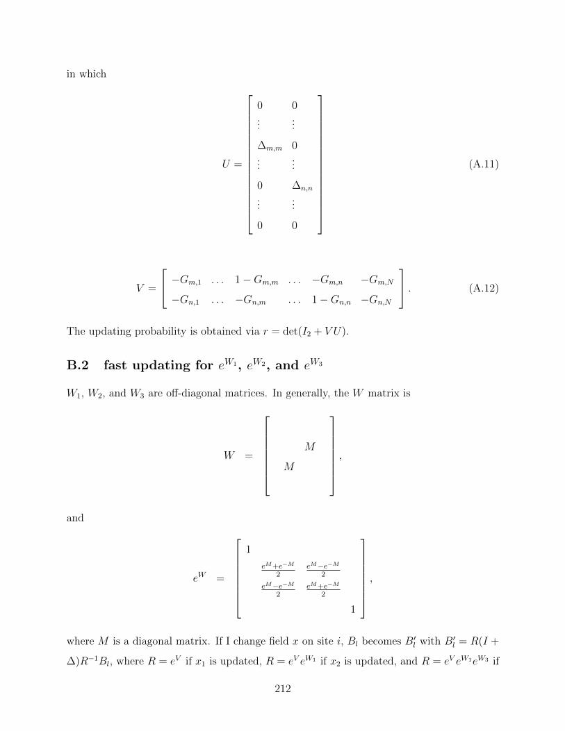
in which

U =

0 0...

...

∆m,m 0...

...

0 ∆n,n

......

0 0

(A.11)

V =

−Gm,1 . . . 1−Gm,m . . . −Gm,n −Gm,N

−Gn,1 . . . −Gn,m . . . 1−Gn,n −Gn,N

. (A.12)

The updating probability is obtained via r = det(I2 + V U).

B.2 fast updating for eW1, eW2, and eW3

W1, W2, and W3 are off-diagonal matrices. In generally, the W matrix is

W =

M

M

,

and

eW =

1

eM+e−M

2eM−e−M

2

eM−e−M2

eM+e−M

2

1

,

where M is a diagonal matrix. If I change field x on site i, Bl becomes B′l with B′l = R(I +

∆)R−1Bl, where R = eV if x1 is updated, R = eV eW1 if x2 is updated, and R = eV eW1eW3 if

212

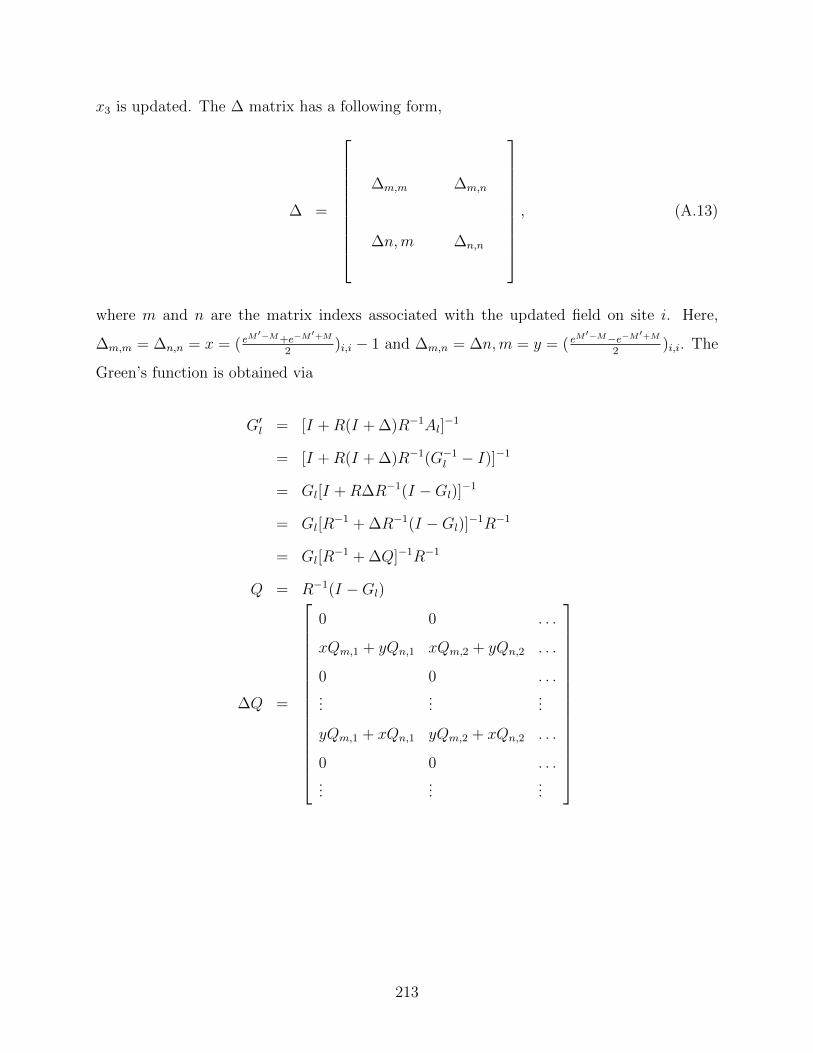
x3 is updated. The ∆ matrix has a following form,

∆ =

∆m,m ∆m,n

∆n,m ∆n,n

, (A.13)

where m and n are the matrix indexs associated with the updated field on site i. Here,

∆m,m = ∆n,n = x = ( eM′−M+e−M

′+M

2)i,i − 1 and ∆m,n = ∆n,m = y = ( e

M′−M−e−M′+M2

)i,i. The

Green’s function is obtained via

G′l = [I +R(I + ∆)R−1Al]−1

= [I +R(I + ∆)R−1(G−1l − I)]−1

= Gl[I +R∆R−1(I −Gl)]−1

= Gl[R−1 + ∆R−1(I −Gl)]

−1R−1

= Gl[R−1 + ∆Q]−1R−1

Q = R−1(I −Gl)

∆Q =

0 0 . . .

xQm,1 + yQn,1 xQm,2 + yQn,2 . . .

0 0 . . ....

......

yQm,1 + xQn,1 yQm,2 + xQn,2 . . .

0 0 . . ....

......

213

=

0 0...

...

x y...

...

y x...

...

Qm,1 Qm,2 . . .

Qn,1 Qn,2 . . .

= UV

Then

G′l = Gl(R−1 + UI2V )−1R−1

= Gl[R−RU(I2 + V RU)−1V R]R−1

= Gl[I −RU(I2 + V RU)−1V ].

The updating probability is

r = coeff × det|R(R + UI2V )|

= coeff × det|I2 + V RU, |

where coeff = e−πx′2

e−πx2 .

214

Appendix B

Applications of the Migdal theory to

the three-orbital SSH model

Before applying the Migdal theory, I need to rewrite the Hamiltonian in the momentum

space. First I do the Fourier transformation of operators,

sk,σ =1√N

∑r

e−ik·rsr,σ (B.1)

pk,x,σ =1√N

∑r

e−ik·(r+a/2)pr,x,σ (B.2)

pk,y,σ =1√N

∑r

e−ik·(r+b/2)pr,y,σ (B.3)

ak =Ω

2~∑r

[√M

NXr+a

2e−ik(r+a

2) − 1

Ω√NM

Pr+a2,xe−ik(r+a

2)

](B.4)

bk =Ω

2~∑r

[√M

NYr+b

2e−ik(r+b

2) − 1

Ω√NM

Pr+a2,ye−ik(r+b

2)

]. (B.5)

Then I have sk+G,σ = sk,σ, pk+G,x,σ = e−iG·a/2pk,x,σ, pk+G,y,σ = e−iG·b/2pk,y,σ, ak+G =

e−iG·a/2ak, and bk+G = e−iG·b/2bk. Hence, pk,x,σ, pk,y,σ, ak, and bk don’t have translation

symmetry. Here, G is the reciprocal lattice vector, a and b are the primitive vector along

x- and y-directions, respectively. If I define the Green’s function as

Gγγ′(r) =1

N

∑u

〈γu+r,σγ′†u,σ〉 (B.6)

215

Gγγ′(k) =∑r

Gγγ′(r)e−ik·r, (B.7)

gγγ′(k) = 〈γk,σγ′†k,σ〉 (B.8)

then

Gss(k) = 〈sk,σs†k,σ〉 = gss(k) (B.9)

Gspx(k) = e−ik·a/2〈sk,σp†k,x,σ〉 = gspx(k)e−ik·a/2 (B.10)

Gspy(k) = e−ik·b/2〈sk,σp†k,y,σ〉 = gspy(k)e−ik·b/2 (B.11)

Gpxs(k) = eik·a/2〈pk,x,σs†k,σ〉 = gpxs(k)eik·a/2 (B.12)

Gpxpx(k) = 〈pk,x,σp†k,x,σ〉 = gpxpx(k) (B.13)

Gpxpy(k) = eik·(a/2−b/2)〈pk,x,σp†k,y,σ〉 = gpxpy(k)eik·(a/2−b/2) (B.14)

Gpys(k) = eik·b/2〈pk,y,σs†k,σ〉 = gpys(k)eik·b/2 (B.15)

Gpypx(k) = e−ik·(a/2−b/2)〈pk,y,σp†k,x,σ〉 = gpypx(k)e−ik·(a/2−b/2) (B.16)

Gpypy(k) = 〈pk,y,σp†k,y,σ〉 = gpypy(k) (B.17)

Daa(q) = daa(q) (B.18)

Dab(q) = dab(q)eiq·(a/2−b/2) (B.19)

Dba(q) = dba(q)e−iq·(a/2−b/2) (B.20)

Dbb(q) = dbb(q) (B.21)

Gγγ′(k) has a translation symmetry. For example,

Gspx(k) =∑r

Gspx(r)e−ik·r

=∑r

1

N

∑u

〈su+r,σp†u+a

2,x,σ〉e

−ik·r

=∑r

1

N

∑u

∑k1,k2

1

N〈sk,σp

†k,x,σ〉e

i(k1−k2)·uei(k1−k)·re−ik2·a2

= 〈sk,σp†k,x,σ〉e

−ik·a2 (B.22)

Gspx(k + G) = 〈sk+G,σp†k+G,x,σ〉e

−i(k+G)·a2

= 〈sk,σp†k,x,σ〉e

iG·a/2e−i(k+G)·a2

216

= Gspx(k) (B.23)

In the momentum space, the Hamiltonian is

H0 =∑k,σ

i2t0sp

(sin(k · a/2)s†k,σpk,x,σ + sin(k · b/2)s†k,σpk,y,σ − h.c.

)+

∑k,σ

4tppsin(k · a/2)sin(k · b/2)(p†k,x,σpk,y,σ + h.c.

)+

∑k,σ

[(∆s − µ) s†k,σsk,σ + (∆p − µ)

(p†k,x,σpk,x,σ + p†k,y,σpk,y,σ

)](B.24)

Hph = ~Ω∑q

[a†qaq + b†qbq

](B.25)

He−ph = αtsp

√~

2NMΩ

∑k1,k2,σ

(ak1−k2

+ a†k2−k1

)[2cos

(k1 · a

2

)s†k1,σ

pk2,x,σ+

2cos

(k2 · a

2

)p†k1,x,σ

sk2,σ

]+(bk1−k2

+ b†k2−k1

)[2cos

(k1 · b

2

)s†k1,σ

pk2,y,σ+ 2cos

(k2 · b

2

)p†k1,y,σ

sk2,σ

], (B.26)

in which ~Ω =√

2KM

and M is the oxygen mass. For conveince, I define α√

12Nω

=

αtsp

√~

2NMΩ, where α = αtsp~√

Mand ω = ~Ω. He−ph can be written in a matrix format

as

He−ph =α√

2ωN

∑k1,k2,σ

(s†k1,σ

p†k1,x,σp†k1,y,σ

)Ak1−k2

0 2cos

(k1·a

2

)0

2cos(k2·a

2

)0 0

0 0 0

+Bk1−k2

0 0 2cos

(k1·b

2

)0 0 0

2cos(k2·b

2

)0 0

sk2,σ

pk2,x,σ

pk2,y,σ

, (B.27)

where Ak = ak + a†k and Bk = bk + b†k.

217

A Self-energy

Feynman diagrams of the Migdal theory is show in Fig. B.1. The electron self-energy is

given by

Σ(k, iωn) = − α2

2Nβω

∑k′,m

daa(k− k′, iωn − iωm)×4cos2(kx/2)gpxpx(k

′, iωm) 4cos(kx/2)cos(k′x/2)gpxs(k′, iωm) 0

4cos(kx/2)cos(k′x/2)gspx(k′, iωm) 4cos2(k′x/2)gss(k

′, iωm) 0

0 0 0

+dab(k− k′, iωn − iωm)×

4cos(kx/2)cos(ky/2)gpxpy(k′, iωm) 0 4cos(kx/2)cos(k′y/2)gpxs(k

′, iωm)

4cos(ky/2)cos(k′x/2)gspy(k′, iωm) 0 4cos(k′x/2)cos(k′y/2)gss(k

′, iωm)

0 0 0

+dba(k− k′, iωn − iωm)×

4cos(kx/2)cos(ky/2)gpypx(k′, iωm) 4cos(ky/2)cos(k′x/2)gpys(k

′, iωm) 0

0 0 0

4cos(kx/2)cos(k′y/2)gspx(k′, iωm) 4cos(k′x/2)cos(k′y/2)gss(k

′, iωm) 0

+dbb(k− k′, iωn − iωm)×

4cos2(ky/2)gpypy(k′, iωm) 0 4cos(ky/2)cos(k′y/2)gpys(k

′, iωm)

0 0 0

4cos(ky/2)cos(k′y/2)gspy(k′, iωm) 0 4cos2(k′y/2)gss(k

′, iωm)

= − α2

2Nβω

∑k′,m

∑k′,m

Daa(k− k′, iωn − iωm)×4cos2(kx/2)Gpxpx(k

′, iωm) 4cos(kx/2)cos(k′x/2)e−ik′x2 Gpxs(k

′, iωm) 0

4cos(kx/2)cos(k′x/2)eik′x2 Gspx(k

′, iωm) 4cos2(k′x/2)Gss(k′, iωm) 0

0 0 0

+Dab(k− k′, iωn − iωm)e−i

kx−ky2 ×

4cos(kx/2)cos(ky/2)Gpxpy(k′, iωm) 0 4cos(kx/2)cos(k′y/2)e−i

k′y2 Gpxs(k

′, iωm)

4cos(ky/2)cos(k′x/2)eik′x2 Gspy(k

′, iωm) 0 4cos(k′x/2)cos(k′y/2)eik′x−k

′y

2 Gss(k′, iωm)

0 0 0

218

Figure B.1: (color online) Feynman diagrams of the Migdal theory. γ, γ′, γ1, γ2, γ3,γ4 areorbital indexs. The solid line indicates electron Green’s function and the wave line indicatesphonon Green’s function. The single line and double line indicate bare and dressed Green’sfunction, respectively.

219

+Dba(k− k′, iωn − iωm)eikx−ky

2 ×4cos(kx/2)cos(ky/2)Gpypx(k

′, iωm) 4cos(ky/2)cos(k′x/2)e−ik′x2 Gpys(k

′, iωm) 0

0 0 0

4cos(kx/2)cos(k′y/2)eik′y2 Gspx(k

′, iωm) 4cos(k′x/2)cos(k′y/2)e−ik′x−k

′y

2 Gss(k′, iωm) 0

+Dbb(k− k′, iωn − iωm)×

4cos2(ky/2)Gpypy(k′, iωm) 0 4cos(ky/2)cos(k′y/2)e−i

k′y2 Gpys(k

′, iωm)

0 0 0

4cos(ky/2)cos(k′y/2)eik′y2 Gspy(k

′, iωm) 0 4cos2(k′y/2)Gss(k′, iωm)

.(B.28)

The Hartree term is given by

ΣH(k, iωn) =

0 ΣH

spx(k, iωn) ΣHspy(k, iωn)

ΣHpxs(k, iωn), 0 0

ΣHpys(k, iωn) 0 0

, (B.29)

where

ΣHpxs(k, iωn) = ΣH

spx(k, iωn)

=2a2

2NωβD0aa(0, 0)2cos(

kx2

)∑k′,m

2cos(k′x2

)

[eik′x2 Gspx(k

′, iωn)

+e−ik′x2 Gpxs(k

′, iωn)

],

and

ΣHpys(k, iωn) = ΣH

spy(k, iωn)

=2a2

2NωβD0bb(0, 0)2cos(

ky2

)∑k′,m

2cos(k′y2

)

[eik′y2 Gspy(k

′, iωn)

+e−ik′y2 Gpys(k

′, iωn)

].

220

Here, D0aa(k, iωn) and D0

bb(k, ivn) are the bare Green’s functions for phonons a and b,

respectively. ωn = (2n+1)πβ

and vn = 2nπβ

are the Matsubara frequency for fermions and

bosons, respectively.

The phonon self-energy is given by

Π(q, iνn) =

Πaa(q, iνn) Πab(q, iνn)

Πba(q, iνn) Πbb(q, iνn)

(B.30)

where

Πaa(q, iνn) =2α2

2Nβω

∑k,m

[2cos(

kx2

)gpxs(k, iωm)2cos(kx + qx

2)gpxs(k + q, iωm + iνn)+

2cos(kx2

)gspx(k, iωm)2cos(kx + qx

2)gspx(k + q, iωm + iνn) +

4cos2(kx2

)gss(k, iωm)gpxpx(k + q, iωm + iνn) +

gpxpx(k, iωm)4cos2(kx + qx

2)gss(k + q, iωm + iνn)

]=

2α2

2Nβω

∑k,m

[2cos(

kx2

)e−i kx2 Gpxs(k, iωm)2cos(

kx + qx2

)e−i kx+qx2 ×

Gpxs(k + q, iωm + iνn) + 2cos(kx2

)ei kx2 Gspx(k, iωm)2cos(

kx + qx2

)ei kx+qx2 ×

Gspx(k + q, iωm + iνn) + 4cos2(kx2

)Gss(k, iωm)Gpxpx(k + q, iωm + iνn) +

Gpxpx(k, iωm)4cos2(kx + qx

2)Gss(k + q, iωm + iνn)

], (B.31)

Πab(q, iνn) =2α2

2Nβω

∑k,m

[2cos(

kx2

)gpys(k, iωm)2cos(ky + qy

2)gpxs(k + q, iωm + iνn)+

2cos(ky2

)gspx(k, iωm)2cos(kx + qx

2)gspy(k + q, iωm + iνn) +

gpypx(k, iωm)4cos(kx + qx

2)cos(

ky + qy2

)gss(k + q, iωm + iνn) +

4cos(kx2

)cos(ky2

)gss(k, iωm)gpxpy(k + q, iωm + iνn)

]=

2α2

2Nβωe−i

qx−qy2

∑k,m

[2cos(

kx2

)e−i kx2 Gpys(k, iωm)2cos(

ky + qy2

)e−iky+qy

2 ×

221

Gpxs(k + q, iωm + iνn) + 2cos(ky2

)eiky2 Gspx(k, iωm)2cos(

kx + qx2

)ei kx+qx2 ×

Gspy(k + q, iωm + iνn) +Gpypx(k, iωm)4cos(kx + qx

2)ei kx+qx

2 ×

cos(ky + qy

2)e−i

k+y+qy2 Gss(k + q, iωm + iνn) + 4cos(

kx2

)e−i kx2 cos(

ky2

)×

eiky2 Gss(k, iωm)Gpxpy(k + q, iωm + iνn)

], (B.32)

Πba(q, iνn) =2α2

2Nβω

∑k,m

[2cos(

kx2

)gspy(k, iωm)2cos(ky + qy

2)gspx(k + q, iωm + iνn)+

2cos(ky2

)gpxs(k, iiωωm)2cos(kx + qx

2)gpys(k + q, iωm + iνn) +

gpxpy(k, iωm)4cos(kx + qx

2)cos(

ky + qy2

)gss(k + q, iωm + iνn) +

4cos(kx2

)cos(ky2

)gss(k, iωm)gpypx(k + q, iωm + iνn)

]=

2α2

2Nβωeiqx−qy

2

∑k,m

[2cos(

kx2

)ei kx2 Gspy(k, iωm)2cos(

ky + qy2

)eiky+qy

2 ×

Gspx(k + q, iωm + iνn) + 2cos(ky2

)e−iky2 Gpxs(k, iωm)2cos(

kx + qx2

)e−i kx+qx2 ×

Gpys(k + q, iωm + iνn) +Gpxpy(k, iωm)4cos(kx + qx

2)e−i kx+qx

2 cos(ky + qy

2)

eik+y+qy

2 Gss(k + q, iωm + iνn) + 4cos(kx2

)ei kx2 cos(

ky2

)e−iky2 Gss(k, iωm)×

Gpypx(k + q, iωm + iνn)], (B.33)

Πbb(q, iνn) =2α2

2Nβω

∑k,m

[2cos(

ky2

)gpys(k, iωm)2cos(ky + qy

2)gpys(k + q, iωm + iνn)+

2cos(ky2

)gspy(k, iωm)2cos(ky + qy

2)gspy(k + q, iωm + iνn) +

4cos2(ky2

)gss(k, iωm)gpypy(k + q, iωm + iνn) +

gpypy(k, iωm)4cos2(ky + qy

2)gss(k + q, iωm + iνn)

]=

2α2

2Nβω

∑k,m

[2cos(

ky2

)e−iky2 Gpys(k, iωm)2cos(

ky + qy2

)e−iky+qy

2 ×

Gpys(k + q, iωm + iνn) + 2cos(ky2

)eiky2 Gspy(k, iωm)2cos(

ky + qy2

)eiky+qy

2 ×

222

Gspy(k + q, iωm + iνn) + 4cos2(ky2

)Gss(k, iωm)Gpypy(k + q, iωm + iνn)

+Gpypy(k, iωm)4cos2(ky + qy

2)Gss(k + q, iωm + iνn)

]. (B.34)

B Charge and superconducting susceptibility

The charge-density-wave susceptibility is defined as

χαβ(q) =1

N

∑r,r′,σ,σ′

eiq·(r−r′)∫ β

0

dτ [〈nr,α,σ(τ)nr′,β,σ′(0)〉 − 〈nr,α,σ(τ)〉〈nr′,β,σ′〉] , (B.35)

in which α and β are orbital indexes. For the noninteracting Hamiltonian, χαβ(q) =

2Nβ

∑k,nGαβ(k + q, iωn)Gβα(k, iωn). Since Gαβ(k, iωn) has a translation symmetry, χαβ(q)

has a translation symmetry as well. χ(q) is a 3× 3 matrix, which could be written as

χ(q) =

χss(q) ei qx

2 χspx(q) eiqy2 χspy(q)

e−i qx2 χpxs(q) χpxpx(q) e−i

qx−qy2 χpxpy(q)

e−iqy2 χpys(q) ei

qx−qy2 χpypx(q) χpypy(q)

. (B.36)

Here, χαβ(q) = 2Nβ

∑k,n gαβ(k + q, iωn)gβα(k, iωn) for the non-interacting system. χαβ(q) is

introduced here in that I can obtain χαβ(q) directly from the Feynman diagram. With the

Migdal theory,

χαβ(q) = χ0αβ(q) +Rα(q)

[II − Π(q, 0)D0(q, 0)

]−1Qβ(q), (B.37)

where D0(q, 0) is the bare phonon Green’s function and II is a 2 × 2 unit matrix. Rα(q)

and QTβ (q) are 1× 2 vectors,

Rα(q) =2α√

2NβωNβ

[D0aa(q, 0)R1

α(q) D0bb(q, 0)R2

α(q)]

(B.38)

QTβ (q) = − 2α√

2Nβω

[Q1β(q) Q2

β(q)]. (B.39)

223

R1s(q) =

∑k,m

[2cos(

kx + qx2

)gss(k + q, iωm)gpxs(k, iωm)

+2cos(kx2

)gspx(k + q, iωm)gss(k, iωm)

]= ei qx

2

∑k,m

[2cos(

kx + qx2

)e−i kx+qx2 Gss(k + q, iωm)Gpxs(k, iωm)+

Gspx(k + q, iωm)2cos(kx2

)ei kx2 Gss(k, iωm)

]R2s(q) =

∑k,m

[2cos(

ky + qy2

)gss(k + q, iωm)gpys(k, iωm)

+2cos(ky2

)gspy(k + q, iωm)gss(k, iωm)

]= ei

qy2

∑k,m

[2cos(

ky + qy2

)e−iky+qy

2 Gss(k + q, iωm)Gpys(k, iωm)+

Gspy(k + q, iωm)2cos(ky2

)eiky2 Gss(k, iωm)

]R1px(q) =

∑k,m

[2cos(

kx + qx2

)gpxs(k + q, iωm)gpxpx(k, iωm) + 2cos(kx2

)gpxpx(k + q, iωm)×

gspx(k, iωm)]

=∑k,m

[2cos(

kx + qx2

)e−i kx+qx2 Gpxs(k + q, iωm)Gpxpx(k, iωm)+

Gpxpx(k + q, iωm)2cos(kx2

)ei kx2 Gspx(k, iωm)

]R2px(q) =

∑k,m

[2cos(

ky + qy2

)gpys(k + q, iωm)gpypx(k, iωm) + 2cos(ky2

)gpxpy(k + q, iωm)×

gspx(k, iωm)]

= e−iqx−qy

2

∑k,m

[2cos(

ky + qy2

)e−iky+qy

2 Gpxs(k + q, iωm)Gpypx(k, iωm)

+Gpxpy(k + q, iωm)2cos(ky2

)eiky2 Gspx(k, iωm)

]R1py(q) =

∑k,m

[2cos(

kx + qx2

)gpys(k + q, iωm)gpxpy(k, iωm) + 2cos(kx2

)gpypx(k + q, iωm)×

gspy(k, iωm)]

= eiqx−qy

2

∑k,m

[2cos(

kx + qx2

)e−i kx+qx2 Gpys(k + q, iωm)Gpxpy(k, iωm)

224

+Gpypx(k + q, iωm)2cos(kx2

)ei kx2 Gspy(k, iωm)

]R2py =

∑k,m

[2cos(

ky + qy2

)gpys(k + q, iωm)gpypy(k, iωm) + 2cos(ky2

)gpypy(k + q, iωm)×

gspy(k, iωm)]

=∑k,m

[2cos(

ky + qy2

)e−iky+qy

2 Gpys(k + q, iωm)Gpypy(k, iωm)

+Gpypy(k + q, iωm)2cos(ky2

)eiky2 Gspy(k, iωm)

]

Q1s(q) =

∑k,m

[2cos(

kx2

)gpxs(k + q, iωm)gss(k, iωm) + 2cos(kx + qx

2)gss(k + q, iωm)×

gspx(k, iωm)]

= e−i qx2

∑k,m

[Gpxs(k + q, iωm)2cos(

kx2

)e−i kx2 Gss(k, iωm)+

2cos(kx + qx

2)ei kx+qx

2 Gss(k + q, iωm)Gspx(k, iωm)

]Q2s(q) =

∑k,m

[2cos(

ky2

)gpys(k + q, iωm)gss(k, iωm) + 2cos(ky + qy

2)gss(k + q, iωm)×

gspy(k, iωm)]

= e−iqy2

∑k,m

[Gpys(k + q, iωm)2cos(

ky2

)e−iky2 Gss(k, iωm)+

2cos(ky + qy

2)ei

ky+qy2 Gss(k + q, iωm)Gspy(k, iωm)

]Q1px(q) =

∑k,m

[2cos(

kx2

)gpxpx(k + q, iωm)gpxs(k, iωm) + 2cos(kx + qx

2)gspx(k + q, iωm)×

gpxpx(k, iωm)]

=∑k,m

[Gpxpx(k + q, iωm)2cos(

kx2

)e−i kx2 Gpxs(k, iωm)+

2cos(kx + qx

2)ei kx+qx

2 Gspx(k + q, iωm)Gpxpx(k, iωm)

]Q2px(q) =

∑k,m

[2cos(

ky2

)gpypx(k + q, iωm)gpxs(k, iωm) + 2cos(ky + qy

2)gspx(k + q, iωm)×

gpxpy(k, iωm)]

225

= eiqx−qy

2

∑k,m

[Gpypx(k + q, iωm)2cos(

ky2

)e−iky2 Gpxs(k, iωm)+

2cos(ky + qy

2)ei

ky+qy2 Gspx(k + q, iωm)Gpxpy(k, iωm)

]Q1py(q) =

∑k,m

[2cos(

kx2

)gpxpy(k + q, iωm)gpys(k, iωm) + 2cos(kx + qx

2)gspy(k + q, iωm)×

gpypx(k, iωm)]

= e−iqx−qy

2

∑k,m

[Gpxpy(k + q, iωm)2cos(

kx2

)e−i kx2 Gpys(k, iωm)+

2cos(kx + qx

2)ei kx+qx

2 Gspy(k + q, iωm)Gpypx(k, iωm)

]Q2py(q) =

∑k,m

[2cos(

ky2

)gpypy(k + q, iωm)gpys(k, iωm) + 2cos(ky + qy

2)gspy(k + q, iωm)×

gpypy(k, iωm)]

=∑k,m

[Gpypy(k + q, iωm)2cos(

ky2

)e−iky2 Gpys(k, iωm)+

2cos(ky + qy

2)ei

ky+qy2 Gspy(k + q, iωm)Gpypy(k, iωm)

]

The superconducting susceptibility is defined as

χspαβ =1

N

∫ β

0

dτ∑r,r′

〈αr,↑(τ)αr,↓(τ)β†r′,↑(0)β†r′,↓(0)〉

=1

N3

∫ β

0

dτ∑r,r′

∑k1,k2,k3,k4

〈αk1,↑(τ)αkk2,↓(τ)β†k3,↑(0)β†k4,↓(0)〉e−i(k1+k2)·re−i(k3+k4)·r′

=1

N

∫ β

0

dτ∑k1,k2

〈αk1,↑(τ)α−k1,↓(τ)β†k2,↑(0)β†−k2,↓(0)〉

=1

N

∫ β

0

dτ∑k

gαβ(k, τ)gαβ(−k, τ)

=1

Nβ

∑k,m

gαβ(k, iωm)gαβ(−k,−iωm)

=1

Nβ

∑k,m

Gαβ(k, iωm)Gαβ(−k,−iωm) (B.40)

226

Within the Migdal theory, χspαβ is given by summing the infinite series of ladder diagrams.

The result is

χspαβ =1

Nβ

∑k,m

Fαβαβ(k, iωm)Λαβαβ(k, iωm), (B.41)

where

Fτ1γ1τ2γ2(k, iωm) = Gτ1γ1(k, iωm)Gτ2γ2(−k,−iωm), (B.42)

fτ1γ1τ2γ2(k, iωm) = gτ1γ1(k, iωm)gτ2γ2(−k,−iωm). (B.43)

Λαβαβ(k, iωm) is the solution of the vertex equation:

fτ1sτ2s(k, iωm)Λτ1sτ2s(k, iωm) = fτ1sτ2s(k, iωm)− α2

2Nβω

∑k′,m′

Daa(k− k′, iωm − iωm′)×[

4cos2(kx2

)fτ1sτ2s(k, iωm)Fpxspxs(k′, iωm′)Λpxspxs(k

′, iωm′) +

fτ1pxτ2px(k, iωm)4cos2(k′x2

)Fssss(k′, iωm′)Λssss(k

′, iωm′) +

2cos(kx2

)fτ1sτ2px(k, iωm)2cos(k′x2

)e−ik′x2 Fpxsss(k

′, iωm′)Λpxsss(k′, iωm′) +

2cos(kx

2)fτ1pxτ2s(k, iωm)2cos(

k′x2

)eik′x2 Fsspxs(k

′, iωm′)Λsspxs(k′, iωm′)

]+Dab(k− k′, iωm − iωm′)e

−ikx−ky

2 ×[4cos(

kx2

)cos(ky2

)fτ1sτ2s(k, iωm)Fpxspys(k′, iωm′)Λpxspys(k

′, iωm′) +

fτ1pxτ2py(k, iωm)4cos(k′x2

)cos(k′y2

)eik′x−k

′y

2 Fssss(k′, iωm′)Λssss(k

′, iωm′) +

2cos(kx2

)fτ1sτ2py(k, iωm)2cos(k′y2

)e−ik′y2 Fpxsss(k

′, iωm′)Λpxsss(k′, iωm′) +

2cos(ky2

)fτ1pxτ2s(k, iωm)2cos(k′x2

)eik′x2 Fsspys(k

′, iωm′)Λsspys(k′, iωm′)

]+Dba(k− k′, iωm − iωm′)e

ikx−ky

2 ×[4cos(

kx2

)cos(ky2

)fτ1sτ2s(k, iωm)Fpyspxs(k′, iωm′)Λpyspxs(k

′, iωm′)+

fτ1pyτ2px(k, iωm)4cos(k′x2

)cos(k′y2

)e−ik′x−k

′y

2 Fssss(k′, iωm′)Λssss(k

′, iωm′) +

227

2cos(ky2


)e−ik′x2 Fpysss(k

′, iωm′)Λpysss(k′, iωm′) +

2cos(kx2

)fτ1pyτ2s(k, iωm)2cos(k′y2

)eik′y2 Fsspxs(k

′, iωm′)Λsspxs(k′, iωm′)

]+Dbb(k− k′, iωm − iωm′)×[4cos2(

ky2

)fτ1sτ2s(k, iωm)Fpyspys(k′, iωm′)Λpyspys(k

′, iωm′) +

fτ1pyτ2py(k, iωm)4cos2(k′y2

)Fssss(k′, iωm′)Λssss(k

′, iωm′) +

2cos(ky2


)e−ik′y2 Fpysss(k

′, iωm′)Λpysss(k′, iωm′) +

2cos(ky2


)eik′y2 Fsspys(k

′, iωm′)Λsspys(k′, iωm′)

]

fτ1pxτ2px(k, iωm)Λτ1pxτ2px(k, iωm) = fτ1pxτ2px(k, iωm)

− α2

2Nβω

∑k′,m′

Daa(k− k′, iωm − iωm′)×[

4cos2(kx2

)fτ1sτ2s(k, iωm)Fpxpxpxpx(k′, iωm′)Λpxpxpxpx(k

′, iωm′) +

fτ1pxτ2px(k, iωm)4cos2(k′x2

)Fspxspx(k′, iωm′)Λspxspx(k

′, iωm′) +

2cos(kx2


)e−ik′x2 Fpxpxspx(k

′, iωm′)Λpxpxspx(k′, iωm′) +

2cos(kx

2)fτ1pxτ2s(k, iωm)2cos(

k′x2

)eik′x2 Fspxpxpx(k

′, iωm′)Λspxpxpx(k′, iωm′)

]+Dab(k− k′, iωm − iωm′)e

−ikx−ky

2 ×[4cos(

kx2

)cos(ky2

)fτ1sτ2s(k, iωm)Fpxpxpypx(k′, iωm′)Λpxpxpypx(k

′, iωm′) +

fτ1pxτ2py(k, iωm)4cos(k′x2

)cos(k′y2

)eik′x−k

′y

2 Fspxspx(k′, iωm′)Λspxspx(k

′, iωm′) +

2cos(kx2


)e−ik′y2 Fpxpxspx(k

′, iωm′)Λpxpxspx(k′, iωm′) +

2cos(ky2

)fτ1pxτ2s(k, iωm)2cos(k′x2

)eik′x2 Fspxpypx(k

′, iωm′)Λspxpypx(k′, iωm′)

]+Dba(k− k′, iωm − iωm′)e

ikx−ky

2 ×[4cos(

kx2

)cos(ky2

)fτ1sτ2s(k, iωm)Fpypxpxpx(k′, iωm′)Λpypxpxpx(k

′, iωm′)+

fτ1pyτ2px(k, iωm)4cos(k′x2

)cos(k′y2

)e−ik′x−k

′y

2 Fspxspx(k′, iωm′)Λspxspx(k

′, iωm′) +

228

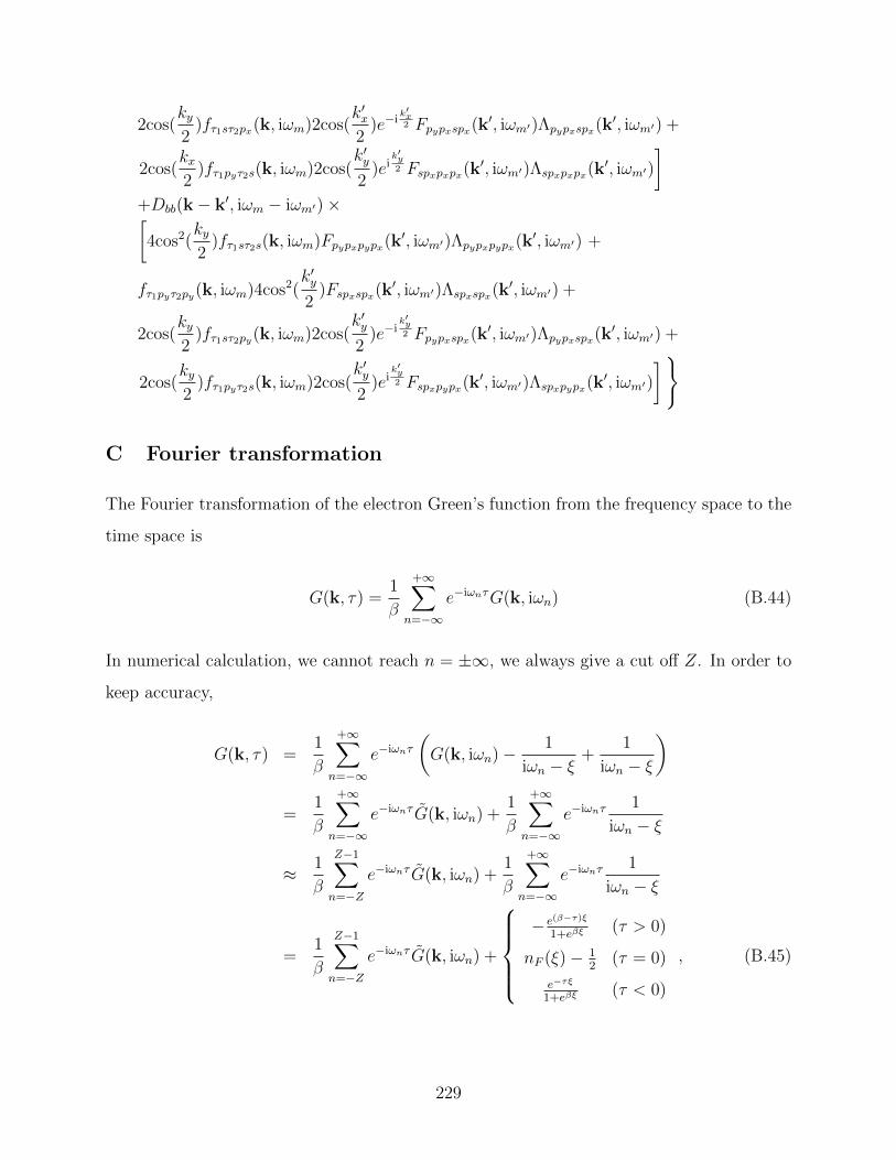
2cos(ky2


)e−ik′x2 Fpypxspx(k

′, iωm′)Λpypxspx(k′, iωm′) +

2cos(kx2


)eik′y2 Fspxpxpx(k

′, iωm′)Λspxpxpx(k′, iωm′)

]+Dbb(k− k′, iωm − iωm′)×[4cos2(

ky2

)fτ1sτ2s(k, iωm)Fpypxpypx(k′, iωm′)Λpypxpypx(k

′, iωm′) +

fτ1pyτ2py(k, iωm)4cos2(k′y2

)Fspxspx(k′, iωm′)Λspxspx(k

′, iωm′) +

2cos(ky2


)e−ik′y2 Fpypxspx(k

′, iωm′)Λpypxspx(k′, iωm′) +

2cos(ky2


)eik′y2 Fspxpypx(k

′, iωm′)Λspxpypx(k′, iωm′)

]

C Fourier transformation

The Fourier transformation of the electron Green’s function from the frequency space to the

time space is

G(k, τ) =1

β

+∞∑n=−∞

e−iωnτG(k, iωn) (B.44)

In numerical calculation, we cannot reach n = ±∞, we always give a cut off Z. In order to

keep accuracy,

G(k, τ) =1

β

+∞∑n=−∞

e−iωnτ

(G(k, iωn)− 1

iωn − ξ+

1

iωn − ξ

)

=1

β

+∞∑n=−∞

e−iωnτ G(k, iωn) +1

β

+∞∑n=−∞

e−iωnτ1

iωn − ξ

≈ 1

β

Z−1∑n=−Z

e−iωnτ G(k, iωn) +1

β

+∞∑n=−∞

e−iωnτ1

iωn − ξ

=1

β

Z−1∑n=−Z

e−iωnτ G(k, iωn) +

− e(β−τ)ξ

1+eβξ(τ > 0)

nF (ξ)− 12

(τ = 0)

e−τξ

1+eβξ(τ < 0)

, (B.45)

229

where ξ is a constant number. The inverse Fourier transformation of the Green’s function is

G(k, iωn) =

∫ β

0

dτeiωnτG(k, τ)

=L−1∑l=0

eiωnτl∆WnG(k, τl)−RneiωnβG(k, β−) +RnG(k, 0+)

=L−1∑l=0

eiωnτl∆WnG(k, τl) +Rn

(G(k, 0+) +G(k, β−)

)=

L−1∑l=0

eiωnτl∆WnG(k, τl) +Rn

(G(k, 0+)−G(k, 0−)

), (B.46)

where ∆ = βL

, Wn = 21−cos(∆ωn)∆2ω2

n, and Rn = −1−i∆ωn−e−i∆ωn

∆ω2n

. Both formulas for the self-

energy and the susceptibility have two summation loops, including adding momentum k and

Matsubara frequency ωn or νn. Doing this summation directly is not efficient. Instead, I can

use the fast Fourier transformation to boost the computing speed. The first step to do the

fast Fourier transformation is changing the equation format using the convolution theory.

For example,

∑k′,m′

D(k− k′, iωm − iωm′)G(k′, iωm) =∑k′,m′

∑r2,r2

e−i(k−k′)·r1e−ik

′·r2

∫ β

0

dτ1ei(ωm−ωm′ )D(r1, τ1)

∫ β

0

dτ2eiωm′τ2G(r2, τ2)

= Nβ∑r

∫ β

0

dτD(r, τ)G(r, τ)eiωnτe−ik·r (B.47)

Here, I use∑

m′ eiωm′ (τ2−τ1) = βδ(τ2 − τ1). Note

D(r, τ) =1

N

∑k

D(k, τ)eik·r

D(k, τ) =1

β

Z∑n=−Z

e−iνnτD(k, iνn)

G(r, τ) =1

N

∑k

G(k, τ)eik·r

G(k, τ) =1

β

Z−1∑n=−Z

e−iωnτG(k, iωn) (B.48)

230

Since G(k, 0+) − G(k, 0−) = −1, the integral of the imaginary time in Eq. B.47 can be

evaluated by

∫ β

0

dτD(r, τ)G(r, τ)eiωnτ = Wn∆L−1∑l=0

eiωnτlD(r, τl)G(r, τl)−RnD(r, 0)δ(r = 0)

The summation in the above equation can be done using the fast Fourier transformation

routine. When I calculate the superconducting susceptibility, there is another integral I

need to consider. That is

∫ β

0

dτD(r, τ)f(r, τ)eiωnτ = Wn∆L−1∑l=0

eiωnτlD(r, τl)f(r, τl)−RnD(r, 0)

[δ(r = (Nx − 1, 0)) + δ(r = (1, 0)) + 2δ(r = 0)] ,

where f(r, τ) = 1N

∑k 4cos2(kx

2)G(k, τ)eik·r When I calculate the phonon self-energy, the

convolution theory is used as the following way,

∑k,m

G(k, iωm)G(k + q, iωm + iνn) = −Nβ∑r

∫ β

0

dτG(R− r, β − τ)G(r, τ)eiνnτe−iq·r,

where R = Nxa +Nyb, N = Nx ×Ny, and

G(R− r, β − τ) =1

N

∑k

G(k, β − τ)e−ik·r

G(k, β − τ) =1

β

∞∑n=−∞

e−iωn(β−τ)G(k, iωn)

= − 1

β

Z−1∑n=−Z

eiωnτ G(k, iωn)− eτξ

1 + eβξ

G(r, τ) =1

N

∑k

G(k, τ)eik·r

G(k, τ) =1

β

Z−1∑n=−Z

e−iωnτ G(k, iωn)− e(β−τ)ξ

1 + eβξ

231

Appendix C

Applications of DQMC to the

three-orbital SSH model

A Three-orbital SSH Model

The full Hamiltonian for the three-orbital Su-Schrieffer-Heeger (SSH) model is H = H0 +

Hlat +He−ph, where

H0 = −tsp∑r,σ

(s†r,σpr,x,σ + s†r,σpr,y,σ + h.c.

)+ tsp

∑r,σ

(s†r+a,σpr,x,σ + s†r+b,σpr,y,σ + h.c.

)+tpp

∑r,σ

(p†r,y,σpr,x,σ − p†r,y,σpr−a,x,σ + p†r−b,y,σpr−a,x,σ − p

†r−b,y,σpr,x,σ + h.c.

)+∑r,σ

[(εs − µ)nr,s,σ + (εp − µ)nr,px,σ + (εp − µ)nr,py ,σ

](C.1)

contains the non-interacting electronic terms of H,

Hlat =∑r

(P 2r,x

2M+MK2X2

r +P 2r,y

2M+MK2Y 2

r

)=∑r

Ω(a†rar + b†rbr + 1

)(C.2)

contains the noninteracting lattice terms, and

He−ph = αt0sp∑r,σ

(Xrs

†r,σpr,x,σ + Yrs

†r,σpr,y,σ + Xrs

†r+a,σpr,x,σ + Yrs

†r+b,σpr,y,σ + h.c.

)(C.3)

232

contains the e-ph coupling terms. Here, s†r,σ(s,σ), p†r,x,σ

(p,x,σ

), p†r,y,σ

(p,y,σ

)are the creation

(annihilation) operators for electrons of spin σ on the Bi 6s, O 2px, and O 2py orbitals at

a coordinate r = (rx, ry), respectively; nr,s,σ = s†r,σsr,σ, nr,px,σ = p†r,x,σpr,x,σ, and nr,py ,σ =

p†r,y,σpr,y,σ are the number operators for s, px, and py orbitals, respectively; εs and εp are the

onsite energies for the 6s orbital and 2p orbital, respectively; µ is the chemical potential.

tsp is the hopping integral between the 6s orbital and 2pγ (γ = x or y) orbital in a uniform

crystal structure. tpp is the hopping integral between 2px and 2py orbitals. α is the e-ph

coupling constant. The movement of the oxygen atoms distorts the uniform crystal structure

and modulates the hopping integral tsp by αtspXr or αtspYr. Pr,x (Pr,y) and Xr (Yr) are the

momentum and displacement operators of oxygen atoms. M is the oxygen mass and K is

the coefficient of elasticity. The bare phonon frequency is defined as Ω =√

2K/M .

B DQMC Procedure

B.1 DQMC algorithm

I use determinant quantum Monte Carlo (DQMC) to study the two-dimensional (2D) three-

orbital SSH model. The details of the method will be discussed in this section. In general,

the finite-temperature expectation value of an observable O is given by

〈O〉 =TrOe−βH

Tre−βH, (C.4)

where the averaging is performed within the grand canonical ensemble. To evaluate 〈O〉, the

imaginary-time interval [0, β] is divided into L discrete steps of length ∆τ = β/L. Then the

partition function can be rewritten using the Trotter formula as

Z = Tr(e−∆τLH

)≈ Tr

(e−∆τHe−phe−∆τK

)L, (C.5)

where K contains the noninteracting terms K = H0 + Hlat. In the Trotter approximation,

terms of order t0sp2α(∆τ)2 and higher have been neglected. This approximation is reasonable

when ∆τ is small.

233

The phonon operators can then be treated in the usual way by inserting a complete set of

position and momentum eigenstates at each time slice. one then integrates out the phonon

momenta. After doing so, the partition function depends on a trace over continuous lattice

displacements Xr,l and Yr,l, and terms that are bilinear in the Fermion operators. The trace

over the former can then be evaluated analytically and expressed as a product of matrix

determinants. The final results is

Within the imaginary-time grid, the position operator Xr (Yr) is replaced with a set

of continuous variables Xr,l (Yr,l). The momentum operators are replaced with a finite

difference Pr,x,l =M(Xr,l+1−Xr,l)

∆τand Pr,y,l =

M(Yr,l+1−Yr,l)∆τ

. The periodic boundary conditions

are enforced on the interval [0, β] such that Xr,L = Xr,0 and Yr,L = Yr,0. In this treatment,

the bare phonon energy of the Hamiltonian Hlat is given by

Z =

∫ ∫dXdY e−Sph∆τdetM↑detM↓, (C.6)

where∫dX and

∫dY are shorthand for integrating over all of continuous phonon

displacements Xr,l and Yr,l. Mσ = I + BσLB

σL−1 · · ·Bσ

1 . Here, I is an N × N identity

matrix and the Bσl matrices are defined as

B↑(↓)l = e−∆τHe−phe−∆τH0 . (C.7)

The lattice term is defined as

Sph =M

2

(Xr,l+1 −Xr,l

∆τ

)2

+M

2

(Yr,l+1 − Yr,l

∆τ

)2

+MK2X2r,l +MK2Y 2

r,l. (C.8)

The integrals over X and Y are evaluated using Metropolis Monte Carlo sample. Here, I

include both single-site and block updates.

Most observables can be expressed in terms of the single particle Green’s function Gσ(τ).

For an electron propagating through field configurations Xr,l and Yr,l, the Green’s

function at time τ = l∆τ is given by

[Gσ(l)]ij = 〈Tτci,σ(τ)c†j,σ(τ)〉 = [I + Aσl ]−1ij , (C.9)

234

where Aσl = Bσl · · ·Bσ

1BσL · · ·Bσ

l+1 and Tτ is the time ordering operator. The determinant of

Mσ is independent of l and is related to the Green’s function on any time slice Gσ(l) by

Mσ = detGσ(l)−1.

B.2 Efficient single-site updates

Equation C.9 shows that the next imaginary-time slice Green’s function Gσ(l + 1) can be

evaluated from the current Green’s function via

Gσ(l + 1) = Bσl+1G

σ(l)[Bσl+1

]−1. (C.10)

This forms the basis for an efficient single-site update scheme. The Monte Carlo starts by

computing the Green’s function on the time slice l = 0 using Eq. C.9. A series of updates

are then proposed for a phonon field at current imaginary-time slice while holding the other

phonon field fixed. For example, one proposes updates Xr,l → X ′r,l = Xr,l + ∆Xr,l while

holding the configuration Yr,l fixed. Then the acceptance probability for this updates is

given by

R = e−∆τ∆EphR↑R↓ = e−∆τ(Eph[X′r,l,Yr,l]−Eph[Xr,l,Yr,l]) detM↑′

detM↑ ×detM↓′

detM↓ , (C.11)

where Mσ′ and Mσ correspond to the phonon fields with and without the proposed updated,

respectively.

After updating a field Xr,l, one has

Bσ(l)→ Bσ′(l) = e−∆τH′e−phe−∆τH0 = e−∆τ(He−ph+V )e−∆τH0 , (C.12)

235

where V is the variation of He−ph after changing a phonon field. Equation C.3 shows V is a

symmetric matrix with only four non-zero elements and it can be written as

V =

. . ....

......

...

· · · 0 αt0sp∆Xr,l 0 · · ·

· · · αt0sp∆Xr,l 0 αt0sp∆Xr,l · · ·

· · · 0 αt0sp∆Xr,l 0 · · ·...

......

.... . .

. (C.13)

To fast calculate the new Bσ′l matrix, I take an approximation as

Bσ′l ≈ e−∆τVBσ

l . (C.14)

This approximation is valid only when ∆τ is small. Then e−∆τV is evaluated via e−∆τV =

Pe−∆τDP T , where P is the eigenstate matrix of V and D is a diagonal matrix with only

two non-zero elements, D1,1 = −√

2αt0sp∆Xr,l and DN,N =√

2αt0sp∆Xr,l. Then the new Bσ′l

matrix can be written as

Bσ′l = Pe−∆τDP TBσ

l = P (I + ∆)P TBσl , (C.15)

where ∆ = 0 except ∆1,1 = e√

2αt0sp∆Xr,l − 1 and ∆N,N = e−√

2αt0sp∆Xr,l − 1.

The new Green’s function after changing a phonon field can be evaluated by

Gσ′l = [I + Aσ′l ]

−1=[I + P (I + ∆)P TAσl

]−1= Gσ

l

[P T + ∆Q

]−1P T , (C.16)

236

where Q = P T (I − Gσl ). Due to the simplicity of the ∆ matrix, ∆Q has only two non-zero

rows,

∆Q =

∆1,1Q1,1 ∆1,1Q1,2 · · · ∆1,1Q1,N

0 0 · · · 0...

......

...

0 0 · · · 0

∆N,NQN,1 ∆N,NQN,2 · · · ∆N,NQN,N

=

∆1,1 0...

...

0 ∆N,N

× Q1,1 Q1,2 · · · Q1,N

QN,1 QN,2 · · · QN,N

= uw, (C.17)

where u and w are N × 2 and 2 × N matrices, respectively. Using the Woodbury matrix

identity and Matrix determinant lemma, the new Green’s function is calculated via

Gσ′l = Gσ

l

[I − Pu(I2 + vPw)−1v

], (C.18)

and the acceptance ratio is given by

Rσ = det|I2 + wPu|, (C.19)

where I2 is a 2 × 2 identity matrix. Once updates have been performed for all fields time

time slice l, Gσ(l) is advanced to Gσ(l + 1) using Eq. C.10 and the process repeated.

This update scheme is efficient although an approximation Bσ′l ≈ e−∆τBσ

l is taken. In

the Sec. B.4 I will compare results from this update with results from an update explicitly

calculating Bσ′l to demonstrate that for a small ∆τ , our approximation can still produce an

exact solution.

B.3 Block updates

In the block update scheme, the lattice displacement for a given site is updated si-

multaneously for imaginary-time slices l. That means the phonon field is updated as

237

Xr,l → Xr,l + ∆Xr or Yr,l → Yr,l + ∆Yr for all l ∈ [0, β]. This type of update helps

to efficiently move the phonon configurations out of false minima at lower temperatures.

However, there is no fast updating formula for the block update and the Green’s function is

required to be calculated from Eq. C.9. Therefore the block update takes a lot of time in

Monte Carlo calculations. To minimize the computing time, I set two to four block updates

at randomly selected sites for every full set of single-site updates to Xr,l and Yr,l.

B.4 Reliability of the fast updates

To assess the reliability of the approximation made in Eq. C.14, I performed two DQMC

calculations. In the first calculation, the updated Green’s function follows each single-site

update and the acceptance ratio is computed via Eq. C.9 and Eq. C.11, respectively. In

this case, the approximation in Eq. C.14 is not taken. In the second calculation, this

approximation is used, and the fast update formulas are used in each single-site update. In

both calculations, the cluster size is set as 2× 2 and the hole density is 〈n〉 = 1. The other

parameters are the same as in chapter 6. Figure C.1 shows that the Green’s functions for

both calculations are the same, indicating ∆τ = β/10 is small enough to produce an exact

solution.

238

0

0.2

0.4

0.6

0.8

G(r

x=

0,r

y=

0)

Gss

(a)Exact

Fast

0

0.2

0.4

0.6

0.8

Gpxpx

(b)

0

0.2

0.4

0.6

0.8

Gpypy

(c)

-0.05

0

0.05

G(r

x=

1,r

y=

0)

Gss(d)

-0.2

-0.1

0

0.1

0.2Gpxpx

(e)

0

0.02

0.04

0.06

Gpypy(f)

-0.05

0

0.05

G(r

x=

0,r

y=

1)

Gss(g)

0

0.02

0.04

0.06

Gpxpx(h)

-0.2

-0.1

0

0.1

0.2Gpypy

(i)

-0.04

-0.02

0

0.02

0 0.2 0.4 0.6 0.8 1

G(r

x=

1,r

y=

1)

Gss(j)

-0.04

-0.02

0

0.02

0 0.2 0.4 0.6 0.8 1

τ/β

Gpxpx(k)

-0.04

-0.02

0

0.02

0 0.2 0.4 0.6 0.8 1

Gpypy(l)

Figure C.1: (color online) Green’s functions as a function of the imaginary time τ fordifferent displacement r = rxa + ryb. a and b are the primitive vectors along x- and y-directions, respectively. The first, second, third columns are the results of Gs,s, Gpx,px , andGpy ,py , respectively. The red circles and blue triangular points represents results from theexact update and the fast update, respectively. Error bars smaller than the marker size havebeen suppressed for clarity.

239

Vita

Shaozhi Li is a PH. D student in the department of Physics and Astronomy at the University

of Tennessee. He works on condensed matter theoretical physics and his major research

interests focus on strongly correlated systems and high-temperature superconductors.

He was born in Zhejiang province, China. He attended Zhejiang Normal University in

2006 in China. After graduation, he headed to the Shandong University for his master degree,

where he started to work on condensed matter theoretical physics. He obtained his master

degree from Shandong University in June, 2013 and went to the University of Tennessee

for his PH. D degree in July. In 2014, he joined Dr. Steve’s group, where he studied the

effect of electron-phonon interactions on strongly correlated systems. As a PH. D student,

Shaozhi Li made many achievements in academic including publishing seven papers. In

2017, he obtained Paul Stelson Fellowships for professional Promise and Allen Fellowship

from the University of Tennessee. Besides, Shaozhi Li attended American Physical Society

(APS) March meeting every year from 2014 to 2018, where he illustrated the importance of

of electron-phonon interactions in high-temperature superconductors.

240

Numerical study of the electron-phonon interaction in ...

Documents

Transcript of Numerical study of the electron-phonon interaction in ...