lable at ScienceDirect

Building and Environment 46 (2011) 1735e1746

Contents lists avai

Building and Environment

journal homepage: www.elsevier .com/locate/bui ldenv

Numerical simulation of dispersion in urban street canyons with avenue-like treeplantings: Comparison between RANS and LES

Salim Mohamed Salim*, Siew Cheong Cheah, Andrew ChanDivision of Environment, Faculty of Engineering, University of Nottingham Malaysia Campus, Semenyih, 43500 Selangor, Malaysia

a r t i c l e i n f o

Article history:Received 17 November 2010Received in revised form28 January 2011Accepted 30 January 2011

Keywords:CFDPollutant DispersionStreet canyonTreesLESRANS

* Corresponding author. Tel.: þ60 389248601; fax:E-mail address: salim@alumni.nottingham.ac.uk (S

0360-1323/$ e see front matter � 2011 Elsevier Ltd.doi:10.1016/j.buildenv.2011.01.032

a b s t r a c t

Previous CFD studies on pollution dispersion problems have largely centred on employing Reynolds-averaged NaviereStokes (RANS) turbulence closure schemes, which have often been reported tooverpredict pollutant concentration levels in comparison to wind tunnel measurement data. In addition,the majority of experimental and numerical investigations have failed to account for the aerodynamiceffects of trees, which can occupy a significant proportion of typical urban street canyons. In the presentwork, the prediction accuracy of pollutant dispersion within urban street canyons of width to heightratio, W/H ¼ 1 lined with avenue-like tree plantings are examined using two steady-state RANS models(the standard k-e and RSM), and Large Eddy Simulation (LES) to compare their performance against windtunnel experiments available on the online database CODASC [1]. Two cases of tree crown porosities areinvestigated, one for a loosely (Pvol ¼ 97.5%) and another for a densely (Pvol ¼ 96%) packed tree crown,corresponding to pressure loss coefficients of l ¼ 80 m�1 and l ¼ 200 m�1, respectively. Results of thetree-lined cases are then compared to a tree-free street canyon in order to demonstrate the impact oftrees on the flow field and pollutant dispersion, and it is observed that the presence of trees reduces thein-canyon circulation and air exchange, and increases the overall concentration levels. Between the twonumerical methods employed, LES performs better than RANS, because it captures the unsteady andintermittent fluctuations of the flow field, and hence, successfully resolves the transient mixing processwithin the canyons.

� 2011 Elsevier Ltd. All rights reserved.

1. Introduction

Air quality is a major concern for residents of dense urban areas,where buildings act as artificial obstacles to wind flow and reducesflow circulation within cities. The flow patterns that developaround individual buildings govern the flow distribution andpollutant dispersion around the building. The superposition andinteraction of flow patterns associated with adjacent buildingsgovern the final distribution of façade pressures and the movementof pollutants in urban and industrial complexes. Traffic emissionscommonly constitute the chief source of air pollution in big citiesand have serious detrimental effects on the population’s health andcomfort. Rapid urbanization and new legislations have resulted inincreased research to enable regulators and urban planners tomitigate pollution problems with the aim of improving citylivability and air quality.

To that effect, a number of experimental and numerical studieshave been performed for the flow and transport of pollutants

þ60 389248017..M. Salim).

All rights reserved.

released about single buildings and clusters of buildings, but thestreet canyon remains the most widely examined configuration inurban air quality problems. The readers are referred to somecomprehensive reviews available in the literature [2e4]. Thesereviews concluded that although considerable progress has beenmade in the CFD community, the current status is far frommeetingthe great needs of assessing and monitoring air quality and muchwork has to be done in order to increase confidence in using CFD asa stand-alone tool. This is due in part to the fact that selection ofa turbulence model greatly influences prediction accuracy ofdispersion processes, which has not been addressed properlybecausemajority of the previous studies have adopted the standardk-e model [5].

Initial studies on the numerical prediction of flow and pollutantdispersion within street canyons were performed using two-dimensional (2D) steady-state Reynolds-averaged NaviereStokes(RANS) equations and their corresponding turbulence closureschemes [6e8]. As computer resources advanced, the investiga-tions were extended to three-dimensional modeling in order tocapture the inherent nature of turbulence, and although improve-ments over 2D modeling were reported, the numerically calculated

S.M. Salim et al. / Building and Environment 46 (2011) 1735e17461736

concentration levels still differed significantly from wind tunnel(WT) and field measurement data [9e11]. In order to address theshortcomings of RANS, Large Eddy Simulation (LES) has beenintroduced in the investigations, resulting in better predictions,with numerically simulated concentration levels matching muchclosely to experimental results [12e14].

RANS models the entire range of eddy length scales and oftenassume gradient transport, which may not be the case for pollutantexchange within street canyons. LES, although computationallymore expensive, has an advantage over RANS in that it explicitlyresolves the majority of the energy carrying eddies and the inter-nally or externally induced periodicity involved, whereas only theuniversally small scale eddies are modeled. Most recently, a studyby Tominaga and Stathopoulous [15] evaluated the model perfor-mance between RANS and LES for the simulation of dispersionaround an isolated building. Another investigation comparing LESagainst RANS for dispersionwithin an urban street canyon has beencarried out by Salim et al. [16]. In both individual studies it wasconcluded that LES not only provided important information on theinstantaneous fluctuations of the flow and concentration fields butperformed better than conventional RANS simulations. This wasbecause LESmanaged to reproduce the unsteady fluctuations aboutthe building and within the street canyon, respectively.

Another important aspect that has been absent in mostinvestigations dealing with air quality problems in urban areas isthe impact of other obstacles such as trees, which can occupya significant proportion of typical urban street canyons. Mochidaet al. [17] reviewed recent achievements in the field of canopyflows and concluded that the presence of trees aerodynamicallydecreases the wind velocity and increases turbulence. The sameobservations were made in the extensive experimental andnumerical studies by Gromke and Ruck [18,19], Gromke et al.[20,21], Buccolieri et al. [22,23] and Balczó et al. [24]. The reportsconcluded that in the presence of trees, both WT measurementsand numerical simulations showed reduced flow velocities andlarger overall pollutant concentrations when compared to theirtree-free counterpart. They attributed these observations mainlydue to the trees blockage effect on the air circulation within thecanyons, which as a result reduced the air exchange and, thus, lesspollutant was dispersed out of the canyons. For their numericalsimulations they employed steady-state RANS and acknowledgedthat although the computational results had good qualitativeagreement with WT measurements, the quantitative agreementwas poor and cited the failure for RANS to capture the transientmixing within the canyons as one of the most probable cause ofthe discrepancy.

In the present work, the numerical performances between RANSand LES are evaluated for the flow field and pollutant dispersionwithin street canyons of W/H ¼ 1 lined with avenue-like treeplantings. The CFD code FLUENT� is used and the advection-diffusion method is employed for dispersion modeling while thetree crowns are represented as porous bodies and line sourcesreplicate traffic exhaust emissions. The relative benefits anddrawbacks of the two numerical approaches are assessed and thecomputational results are compared to concentration measure-ments from WT experiments carried out at the Karlsruhe Instituteof Technology, Germany [1] www.codasc.de. Two cases of treecrown porosities are investigated, one for a loosely (Pvol ¼ 97.5%)and another for a densely (Pvol ¼ 96%) packed model, resulting inpressure loss coefficients of l ¼ 80 m�1 and l ¼ 200 m�1, respec-tively. Finally, numerical results of the presently studied tree-linedcases are compared to a tree-free reference case (which has beenpresented in detail in the work of Salim et al. [16]) to demonstratethe aerodynamic effects of trees on the flow field and pollutantdispersion.

In the RANS simulation, the two-equation standard k-e andseven-equation RSM turbulence models are employed with secondorder upwind scheme, whereas for LES, the dynamic Smagorinsky-Lilly subgrid-scale (SGS) model is implemented.

Majority of the aforementioned studies have already accessedthe merits and drawbacks in the predictions of the flow field andturbulent structures by different numerical models available in CFDcodes. In addition, the aerodynamic effects of trees on the flow fieldand pollutant dispersion within urban street canyons have beenextensively studied [20e24]. Therefore, in the present work,although similar comparisons are made regarding the flow fieldand transport process and the impacts of trees on the flow field inrelation to a tree-free canyon, they are not repeated in detail here.Instead, the main aim of the present work is to demonstrate thecapability of LES to produce better and more consistent predictionsas opposed to conventional RANS. This complements the pool ofresearch work accessing the merits of LES in dispersion modelingand aims to increase confidence in using CFD as an alternative toexperimentation. In addition, the work further reconfirms themechanism of the discrepancy in relation to the overpredictionsobtained from previous RANS computations.

It is also worth noting that most of the published work focusedon presenting the mean pollutant concentration and/or flow fielddata in the mid streamwise direction preventing a detailed evalu-ation of the spatial and temporal performances of the numericaltechniques used (i.e. they did not show the distribution along thefaçades of the buildings). It is also known that WT experimentsusually provide data for limited number of measurement locations.Therefore, besides the mean flow solutions, the three-dimensionaldistribution and time-evolution of the concentration field at thestreet canyon’s leeward and windward walls of the buildings areillustrated in the present study.

2. Numerical method

Description of the different numerical approaches, namelysteady-state RANS and LES have been covered in Salim et al. [16].For the sake of brevity, only important information is repeated here.

2.1. RANS

In steady-state RANS modeling, the flow properties aredisintegrated into their mean and fluctuating components byReynolds decomposition and substituted into the NaviereStokesequations, which on time-averaging yields the RANS equations forincompressible Newtonian fluids as follows:

vuivxi

¼ 0

and

ujvuivxj

¼ �1r

vpvxi

þ yv2uivx2j

� u0jvu0ivxj

ui and u0i are the mean and fluctuating parts of the velocitycomponent ui in the xi-direction, respectively, p is the mean pres-sure, r is the density, and y is the viscosity. Appearance of thefluctuations associated with turbulence give rise to additionalstresses in the fluid, the so-called Reynolds stresses, ru0iu

0j,

which need to be modeled in order to mathematically close theproblem.

In the present study, the standard k-e and RSM models areemployed for the investigation. The main difference between thetwo chosen models is that the standard k-e model assumes the

S.M. Salim et al. / Building and Environment 46 (2011) 1735e1746 1737

Reynolds stresses to be isotropic and solves for only two additionequations: one for the kinetic energy, k and another for thedissipation rate, e. On the other hand, RSM solves for seven extraequations to account for the six individual components of theReynolds stresses and one for dissipation rate, e.

Unsteady RANS (URANS) approach is also available, whichessentially solves the above described transport equations but withan additional unsteady term, for example

vuivt

in the momentum equation

vuivt

þ ujvuivxj

¼ �1r

vpvxi

þ yv2uivx2j

� u0jvu0ivxj

It should be noted that although URANS solves for unsteadiness,they are only applicable to non-stationary flows such as periodic orquasi-periodic flows involving deterministic structures (i.e. oftenexternally induced fluctuations) and falls most often short ofcapturing the remaining large scales, hence, are not a suitablereplacement for LES, and are therefore not employed for the presentstudy because internally induced fluctuations are significant.

2.2. LES

In LES, the large scale eddies are solved directly and only theinfluences of the small scale eddies on the large scale eddies aremodeled unlike in RANS where the entire range of eddies ismodeled. A spatial filtering operation is used to separate the largeand small eddies of the flow, resulting in the filtered continuity andmomentum equations of the incompressible NaviereStokes equa-tions as follows:

vuivxi

¼ 0

and

vuivt

þ ujvuivxj

¼ �1r

vpvxi

þ yv2uivx2j

� vsijvxj

Here, the overbar indicates spatial filtering, and not time-averagingas in RANS. Therefore, ui and p are the filtered velocity and pressure,respectively. Additional tensor terms, sij ¼ uiuj � uiuj are intro-duced due to the filtering operation (analogous to the Reynoldsstresses resulting from Reynolds-averaging) and are commonlytermed the subgrid-scale (SGS) stresses.

FLUENT� employs the Boussinesq hypothesis [25] as in theRANS modeling, computing SGS turbulent stresses from

sij �13skkdij ¼ �2mtSij

where mt is the subgrid-scale turbulent viscosity, and Sij is the rate-of-strain tensor for the resolved scale defined by

Sijh12

vuivxj

þ vujvxi

!

The eddy-viscosity is modeled by

mt ¼ rL2s jSjwhere Ls is the mixing length for the subgrid-scales and

jSjhffiffiffiffiffiffiffiffiffiffiffiffiffi2SijSij

q. In FLUENT�, Ls is computed using

Ls ¼ min�kd;CsV1=3

�

where k is the von Kármán constant (0.4), d is the distance to theclosest wall, Cs is the Smagorinsky constant, and V is the volume ofthe computational cell.

In the present study, the dynamic Smagorinsky-Lilly SGS modelis chosen since no homogeneity exists in the flow. The model,initially conceived by [26] and subsequently by [27] dynamicallycomputes the Smagorinsky constant, Cs, based on the informationprovided by the resolved scales of motion. By employing LES ina complex flow simulation such as the case of flow and pollutanttransport within an urban street canyon, less approximation butmore direct resolving is achieved. The trade-off though, is that LESrequires substantially finer meshes and needs to be run for suffi-ciently longer flow-through times in order to obtain stable statisticsof the flow being modeled. As a result, the computational costassociated with LES is normally in orders of magnitudes higherthan that of steady RANS calculations in terms of memory (RAM)and CPU time.

3. Modeling approach

3.1. Experimental setup

An extensiveWTexperimental database has been established atthe Laboratory of Building and Environmental Aerodynamics,Karlsruhe Institute of Technology (KIT). Concentration data isaccessible to the scientific community online at www.codasc.de.The present numerical simulations replicate the above experi-ments, and the computational results are validated againstmeasurement data. A brief explanation of the WT setup follows.

Flow field and concentrations measurements were performedfor a scale street canyon in an atmospheric boundary layer WT. Aboundary layer flow with mean velocity u(z) profile exponenta ¼ 0.30 and turbulence intensity Iu profile exponent aI ¼ 0.36,according to the power law formula were reproduced in the testsection as follows:

uðZÞu�Zref

� ¼

ZZref

!a

and

IuðZÞIu�Zref

� ¼

ZZref

!�aI

A flow velocity of u(zref ¼ H) ¼ 4.70 ms�1 (H being buildingheight) was obtained. In the test section, a 1:150 scaled model ofan isolated street canyon of length L ¼ 180 m and street widthW ¼ 18 m with two flanking buildings of height H ¼ 18 m andwidth B ¼ 18 m was mounted perpendicular to the approachflow.

Four line sources with Sulfur hexafluoride (SF6) as tracer gaswere incorporated in the model street to simulate the release oftraffic exhausts. The emission rate Q was maintained at 10 gs�1.Mean concentrations of the gas were measured at the canyonwallsand normalized according to

cþ ¼ cuHHQ=l

with c measured concentration, uH flow velocity at height H in theundisturbed approach flow and Q/l tracer gas source strength perunit length.

Fig. 1. Computational domain and boundary conditions for the CFD simulation setup.

S.M. Salim et al. / Building and Environment 46 (2011) 1735e17461738

Positioned along the centre of the model street canyon wereporous tree crowns in order tomimic avenue-like tree planting. Theaerodynamic characteristics of the tree crowns were described bya pressure loss coefficient l [m�1] evaluated in forced convectionconditions according to:

l ¼ Dpstatpdynd

¼ pwindward � pleeward�1=2ru2d

�with Dpstat the difference in static pressure of the windward andleeward sides of the porous obstacle, pdyn the dynamic pressure, uthe mean streamwise velocity and d the porous obstacle thicknessin the streamwise direction. Measurements resulted in pressureloss coefficients of l ¼ 200 m�1 and l ¼ 80 m�1 for the case ofPvol ¼ 96% and Pvol ¼ 97.5%, respectively.

For further details on the experimental setup, results anddiscussion the readers are referred to thework by Gromke and Ruck[18,19].

3.2. Simulation setup

3.2.1. Computational domain and boundary conditionsNumerical simulations were performed with the aim of repro-

ducing the above-described WT experiments focusing on theconcentration distribution within the street canyon in order to

Fig. 2. Velocity and TKE profiles for the inlet boundary condition showing comparison betwe

compare between the accuracy predictions of RANS (standard k-e andRSM) and LES. The study also included an investigation on theaerodynamic effect of trees on the pollutant dispersion by comparingthe presently studied tree-lined cases to the tree-free reference casepreviously investigated in Salim et al. [16]. The computationaldomain and boundary conditions are summarized in Fig. 1.

The domain was discretized using hexahedral elements incor-porating recommendations by Salim et al. [28] with a wall yþ > 30(yþ being the dimensionless wall distance indicating which part ofthe near-wall region of the boundary layer is resolved), determinedto be most suitable for wall functions. From a grid study a meshwith approximately 1.2 million cells was chosen. More than half ofthe total cells (i.e. z 600,000 cells) were placed in the sub-domaindefining the vicinity of the buildings and street canyon (see Fig. 1 e

with a volume of 250 H3) so as to impose a finer mesh resolution inthe region of interest, due to the presence of large gradients in theflow variables i.e. separation, reattachment and recirculation. Theminimum grid spacing was Dx ¼ Dy ¼ Dz ¼ 0.077 H. Cell stretching(i.e. use of successive ratio) was avoided since no homogeneousdirection existed in the flow, and therefore, equal spatial resolutionwas imposed in all directions.

In order to replicate the boundary conditions of the WT exper-iment, a User-Defined Function (UDF) was implemented in the CFDcode. The inlet wind speed was assumed to follow a power lawprofile:

en the simulated profile created using User-Defined Functions and experimental profiles.

S.M. Salim et al. / Building and Environment 46 (2011) 1735e1746 1739

uðzÞ ¼ 4:7� z �0:3

m=s

0:12

Turbulent kinetic energy and dissipation rate profiles werespecified as follows:

k ¼ u2*ffiffiffiffiffiffiCm

p �1� z

d

�

and

e ¼ u3*kZ

�1� Z

d

�

Where d is the boundary layer depth (z0.5 m), u* ¼ 0.54 ms�1 isthe friction velocity (known from log-law curve fitting of WTmean velocity profile), k the von Kàrmàn constant (0.4) andCm ¼ 0.09. The vertical distributions of quantities (specifically, thevelocity profile and TKE) at the inflow boundary conditions arepresented in Fig. 2.

Horizontal homogeneity of the turbulent boundary layer wasachieved with the present boundary conditions on examination inan ‘empty’ computational domain. The term “horizontal

Fig. 3. Positions of line source and tree planting shown for the wind tunnel setup

homogeneity” refers to the absence of streamwise gradients in thevertical profiles of the meanwind speed and turbulence quantities[29,30]. In FLUENT�, the surface roughness is expressed in termsof a sand grain roughness Ks instead of the aerodynamic roughnessz0 as is the case in most meteorological codes. In order tocircumvent problems with a coarse grid resolution near theground due to a large sand grain roughness value Ks, Gromke et al.[20] set Ks equal to aerodynamic roughness length, z0 which wasfound to be z0 ¼ 0.0033 m in the WT experiments. They agree thatsetting Ks equal to z0 was not correct in a strong sense; but justifythe choice from the results obtained. Only minor reduction (about10% of the inlet values) in the velocity profiles up to the location ofthe streamwise building occurred for both k-e and RSM. Thepredicted turbulence intensity tended to become smaller near theground (z/H < 1), where less than 10% change were found.Ks ¼ z0 ¼ 0.0033 m was also defined in the present study, toaccount for the surface roughness, following a similar investiga-tion in an ‘empty’ domain.

FLUENT� inbuilt spectral synthesizer based on the work ofSmirnov et al. [31] was used to synthesize the convergedmean flowsolution obtained from the RANS simulation. This basically super-imposed turbulence on top of the mean flow field in order to

(� CODASC, KIT. www.codasc.de) and corresponding computational domain.

S.M. Salim et al. / Building and Environment 46 (2011) 1735e17461740

translate the initial and boundary conditions defined for the RANSsimulation for use in the LES computation.

3.2.2. Flow simulationThe steady-state RANS mean solutions were obtained using the

standard k-e and RSM turbulence models. Second order upwindnumerical scheme was selected for all the transport equations toreduce numerical diffusion except for pressure, where the Standardinterpolation was used. The scaled residual criteria for all the flowproperties were set at 1 �10�5 and pressure-velocity coupling wasachieved using SIMPLE.

In LES, the dynamic Smagorinsky-Lily SGS model together withbounded central differencing discretization scheme formomentum, second order time-advancement and second orderupwind for species and energy transport equations were selected.PRESTO and SIMPLEC were used for pressure and pressure-velocitycoupling, respectively. Convergences for the scaled residuals wereset at 1 �10�3. This follows recommendations as presented in BestPractices for LES from FLUENT� [32].

Following the work of Cai et al. [13], the turnover time of theprimary circulation, tc, in the canyon is of the order of

Fig. 4. Mean normalized concentration data on Wall A (leeward) and Wall B (windward) sperformed with k-e, RSM and LES simulations for tree crowns with porosity of l ¼ 80 and

tc ¼ W þ HUc

where Uc is the velocity scale of the mean wind in the canyonwhich was found to be w0.14 ms�1 resulting in a value of tc ¼ 2 s.Initially, the simulation was run for 33 flow-through time (T ¼ L/Ub

with L being the streamwise length of the domain and Ub the bulkvelocity) corresponding to 10 tc. Statistically steady-state wasachieved at this point. The flow statistics were then reset, and theflowwas allowed to run for a further 33 flow-through time (¼10 tc)to ensure that the final time-averaged results were independent ofthe initial conditions. A check was performed comparing the meansolutions obtained from an average of 50 flow-through time(¼15 tc) to that of the selected 33 flow-through time (¼10 tc), and itwas observed that both symmetry and mean flow propertymagnitudes did not vary between the two sampling sizes, furthersupporting the fact that the solution had achieved statisticallystationary state and further iterations or reduction in time-stepsize were unnecessary.

Similarly, as with the grid study, temporal resolution sensitivitywas performed and a time-step Dt ¼ 1/8 was selected. The cell

howing comparison between WT data (available from CODASC) and numerical resultsl ¼ 200 respectively.

Fig. 5. Mean concentration profiles at three different locations on a) Wall A and b) Wall B to compare the different numerical results to experimental data (CODASC), for tree crownswith porosity of l ¼ 80 and l ¼ 200 respectively. Legends and axis title are the same for all graphs.

S.M. Salim et al. / Building and Environment 46 (2011) 1735e1746 1741

Courant number was observed to be less than 0.5 within the streetcanyon and in the vicinity of the buildings.

The simulations were performed in parallel on an Intel� Xeon�

workstation (4 CPUs).Numerically predicted vertical flow velocities, w were normal-

ized by the velocity of the undisturbed flow uH according to:

Fig. 6. a) Mean normalized vertical velocity contours, wþ and b) corresponding mean normfor x/H ¼ 9 to 10), comparing k-e, RSM and LES results for tree crown with porosity of l ¼

wþ ¼ wuH

3.2.3. Dispersion modelingThe advection-diffusion (AD) approach was employed for

dispersion of the pollutant, where FLUENT� computes the massdiffusion in turbulent flows as follows:

alized concentration contours, cþ at the mid plane of the street canyon (that is y/H ¼ 080 and l ¼ 200 respectively.

Fig. 7. Instantaneous normalized concentration data on Wall A and Wall B for different time instances obtained by LES, compared to mean (time-averaged) data from WT (CODASC)and LES, for tree crown with porosity of l ¼ 200.

S.M. Salim et al. / Building and Environment 46 (2011) 1735e17461742

J ¼ ��rDþ mt

Sct

�VY

D is the molecular diffusion coefficient for the pollutant in themixture, mt is the turbulent viscosity, Y is the mass fraction of the

Fig. 8. a) Instantaneous normalized vertical velocity contours, wþ and b) corresponding instH ¼ 0 from x/H ¼ 9 to 10) obtained using LES showing the time-evolution (t ¼ 10,20,30 an

pollutant, r is the mixture density. In RANS the turbulentviscosity is computed as mt¼ r (Cmk

2/e)whereas for LES the subgrid-scale turbulent viscosity is used instead. Sct ¼ mt/(rDt) is theturbulent Schmidt number, where Dt is the turbulent diffusivity.Default values of Sct¼ 0.7 were used and fine tuning was avoided as

antaneous normalized concentration contours, cþ at mid plane of the canyon (that is y/d 40 s) and the time-averaged results, for tree crown with porosity of l ¼ 200.

S.M. Salim et al. / Building and Environment 46 (2011) 1735e1746 1743

recommended by Rossi and Iaccarino [33], where they examinedthe literature and determined that altering the turbulent Schmidtnumber was problem dependent and thus not encouraged.

The line sources were simulated by ear-marking sections of thevolume in the geometry and defining them as separate fluid zonesat the required discharge positions (see Fig. 3).

3.2.4. Tree crown modelingSimilar to the line sources, the tree crowns were simulated by

ear-marking section of the volume in the geometry and definingthem as a separate porous zone at the desired position, thenassigning a pressure loss coefficient to this region. In FLUENT�, theporous media model adds a momentum sink to the standard fluidflow equations, incorporating an empirically determined flowresistance in the region of the computational domain (i.e. fluid zonedefined as porous), which were determined to be l ¼ 80 and200 m�1 from the WT measurements, established in previousstudies by Gromke et al. [20] and Buccolieri et al. [22]. The sourceterm (acting as sink in this case) is composed of two parts: a viscousloss term (Darcy, the first term on the right-hand side) and an inertialloss term (the second term on the right-hand side) as follows:

Si ¼ �0@X3

j¼1

Dijmvj þX3j¼1

Cij12rjvjvj

1A

where Si is the source term for the ith (x, y, or z) momentumequation, jvj is the magnitude of the velocity and D and C areprescribed matrices. The momentum sink contributes to createsa pressure drop that is proportional to the fluid velocity (or velocitysquared) in the porous cell. FLUENT�, solves the standard conser-vation equations for turbulence quantities in the porous mediumand turbulence is treated as though the solid medium has no effecton the turbulence generation or dissipation rates.

The position of the trees and line sources in the WT setup andcomputational domain are summarized in Fig. 3.

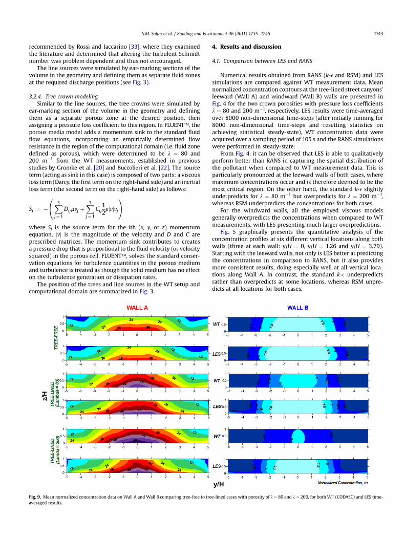
Fig. 9. Mean normalized concentration data on Wall A and Wall B comparing tree-free to treaveraged results.

4. Results and discussion

4.1. Comparison between LES and RANS

Numerical results obtained from RANS (k-e and RSM) and LESsimulations are compared against WT measurement data. Meannormalized concentration contours at the tree-lined street canyons’leeward (Wall A) and windward (Wall B) walls are presented inFig. 4 for the two crown porosities with pressure loss coefficientsl ¼ 80 and 200 m�1, respectively. LES results were time-averagedover 8000 non-dimensional time-steps (after initially running for8000 non-dimensional time-steps and resetting statistics onachieving statistical steady-state), WT concentration data wereacquired over a sampling period of 105 s and the RANS simulationswere performed in steady-state.

From Fig. 4, it can be observed that LES is able to qualitativelyperform better than RANS in capturing the spatial distribution ofthe pollutant when compared to WT measurement data. This isparticularly pronounced at the leeward walls of both cases, wheremaximum concentrations occur and is therefore deemed to be themost critical region. On the other hand, the standard k-e slightlyunderpredicts for l ¼ 80 m�1 but overpredicts for l ¼ 200 m�1,whereas RSM underpredicts the concentrations for both cases.

For the windward walls, all the employed viscous modelsgenerally overpredicts the concentrations when compared to WTmeasurements, with LES presenting much larger overpredictions.

Fig. 5 graphically presents the quantitative analysis of theconcentration profiles at six different vertical locations along bothwalls (three at each wall: y/H ¼ 0, y/H ¼ 1.26 and y/H ¼ 3.79).Starting with the leeward walls, not only is LES better at predictingthe concentrations in comparison to RANS, but it also providesmore consistent results, doing especially well at all vertical loca-tions along Wall A. In contrast, the standard k-e underpredictsrather than overpredicts at some locations, whereas RSM unpre-dicts at all locations for both cases.

e-lined cases with porosity of l ¼ 80 and l ¼ 200, for both WT (CODASC) and LES time-

S.M. Salim et al. / Building and Environment 46 (2011) 1735e17461744

Moving to the windward walls, LES overpredicts the concen-trations at all locations, while the two RANS models start off well atthe centerline (y/H ¼ 0) but then diverges from the experimentaldata towards the street canyons’ ends. One thing that is reiterated isthat LES produces more consistent results (albeit the over-predictions on thewindwardwalls) as opposed to the RANSmodelswhich show varying degree of accuracy at various locations and fordifferent porosities.

To expand on the discussion, the predictions obtained by thedifferent numerical approaches are compared based on the meannormalized velocities and concentration contours along the midplane y/H ¼ 0 within the street canyons. This is demonstrated inFig. 6. The transport and, hence, the distribution of pollutants aredependent on the flow field development. No flow field measure-ments are available from the WT database, but since it has beenestablished that the numerical predictions of the pollutantconcentrations by LES is more consistent and accurate, particularlyfor the leeward walls (where the maximum concentration occur)and a number of previous studies have indicated LES to be moresuperior than RANS when validating flow fields and turbulencestructures against experimental results (see for example[14e16,34,35]), using the LES results as the benchmark for thepurpose of comparison to RANS is justified.

Fig. 10. a) Mean normalized vertical velocity contours, wþ and b) corresponding mean normH ¼ 9 to 10) obtained using LES comparing tree-free to tree-lined cases with porosity of l

Referring to Fig. 6, the differences in concentration levelsbetween the employed numerical methods could be explained bythe fact that the RANS models underpredict the in-canyon flowcirculation strengths for both porosities studied. In other words,lower maximum magnitudes of negative and positive velocitiesare reproduced by RANS as opposed to LES. Furthermore, theRANS models predict an accumulation of pollutant towards theleeward walls, whereas LES produces a greater spread within thecanyon. This could be explained by the fact that LES resolves theunsteady fluctuations and, thus, successfully captures the transientmixing, dispersion and diffusion of airborne materials.

In terms of resource demand and computational cost the stan-dard k-e took about 2 h, RSM took a day and LES two weeks ona similar high performance workstation for each case. But with therichness in details and better predictions, the computational cost ofLES is justified when taking into account the associated cost andtime of an equivalent experimental investigation.

4.2. Instantaneous solution

The WT experiments only provided the mean concentrationdata averaged over a sampling period and, thus, did not reveal theflow field development and corresponding time-evolution of the

alized concentration contours, cþ at mid plane of the canyon (that is y/H ¼ 0 from x/¼ 80 and l ¼ 200 respectively.

S.M. Salim et al. / Building and Environment 46 (2011) 1735e1746 1745

pollutant dispersion. Moreover, majority of the previous numericalstudies on air quality problems have only presented the mean flowequation results without considering the flow statistics (such aswith the case of the RANS models used in the present study).

The LES results in Figs. 7 and 8 (only illustrated for thel¼ 200m�1 case) support the observations by Louka et al. [36] whostrongly recommend the need for resolving the unsteady andintermittent fluctuations of the flow field in order to achieve goodnumerical results. The recommendation is echoed here, where thepeak values of the concentration field is shown to vary significantlywith time.

Looking at Fig. 8a, it can be seen that although the time-aver-aged results show a neat bubble of positive and negative velocitiesat the leeward and windward walls, respectively, the instantaneousflow field fluctuates greatly too. In addition, LES is able to capturepockets of opposing velocities intertwining that promote turbulentmixing resulting in the wider spread witnessed in the in-canyonpollutant distribution, and is one of the underlying reasons why LESproduces better concentration predictions as compared to RANS.

As mentioned earlier, the transport of pollutants is dependenton the flow field development; hence accurate resolution ofturbulent flow fields are paramount to good predictions ofpollutant dispersions. This is successfully achieved by LES. Tofurther illustrate this point, the relationship between the pollutantdispersion and flow field development is presented in Fig. 8.

4.3. Effect of trees (tree-free vs. tree-lined)

The final aim of the present study is to demonstrate the aero-dynamic impact of trees on the flow field and pollutant concen-tration in order to address the importance of accounting for otherlarge obstacles such as trees in CFD studies, so as to achieve more‘realistic’ representations of typical urban scenarios. Figs. 9 and 10show the comparison between a previously studied tree-free case[16] and the present tree-lined canyons’ results.

In Fig. 9, WTmeasurement data are compared to LES results, andit can be seen that for all the three cases, LES reproduce sufficientlyagreeable predictions and resonate a consistency that is absent inRANS models. In terms of the concentration magnitude, it isobserved that in the tree-lined cases the pollutant levels at theleeward walls increases significantly when compared to the tree-free case, whereas the windward walls’ concentrations decreasesslightly. But the difference in concentration between the twodifferent porosities is less prominent as opposed to the disparitybetween the tree-lined and tree-free cases.

Fig. 10 helps explain the above observations by relating the flowdevelopment to the concentration levels. In the presence of trees,the in-canyon flow circulation strength is reduced when comparedto the tree-free canyon, indicated by the reduction in themaximumpositive and negative velocities. This in turn implies that less air isexchanged with the above-roof flow and, thus, less pollutant isdispersed out of the canyon. Between the two porosities, thedensely packed (l ¼ 200 m�1) tree model’s circulation bubble isonly slightly smaller than that of the loosely packed model(l ¼ 80 m�1), resulting in a minor increment in the concentrationlevel, as opposed to the larger difference found between tree-freeand tree-lined canyons.

5. Conclusions

The widely employed steady-state RANS turbulence modelsproduce numerical predictions of qualitative agreement to exper-imental results albeit at varying degree of accuracy for differentmeasurement locations and tree crown porosities, and are notcapable of reciprocating quantitatively the solutions of complex

flow structures with which the dispersion of pollutants depend on.LES significantly improves the flow prediction and, hence, thepollutant dispersion, reproducing better and more consistentresults as compared to RANS. This is because LES captures both theexternal and internal induced periodicity and thus, successfullyresolves the intermittent and unsteady fluctuations of the flowfield. This in turn allows the transient mixing within the streetcanyon to be properly accounted for resulting in better predictionsof the diffusion of pollutants.

LES also provides important information on the instantaneousfluctuations and, thus, are more suitable than RANS for situationswhere detailed predictions are required, such as in the case ofmodeling the deliberate or accidental release of hazardous airbornematerials. However, it should be noted that the enhancements byLES comes with a price, with a computational demand an order ofmagnitude higher than that of the most expensive steady RANScalculations (i.e. RSM).

Another conclusion that can be drawn from the study is that thepresence of other large obstacles such as trees in typical urbanstreet canyons considerably alters the flow field and pollutantconcentration and, therefore, should not be excluded in conven-tional numerical investigations so as to obtain better representa-tion of real urban scenarios. Trees act as obstacles to the wind,reducing air exchange and as a result less pollutant are transportedout of the canyon. These are similar to the original experimentalobservations of Gromke and Ruck [18,19]. It should, however, benoted that only the aerodynamic effect of trees have been takeninto account in the present, and not the biological factors. Similarobservations are expected for other obstacles such as rows ofparked cars, and are left for future investigation.

All in all, LES provides good agreement with measurement data,encouraging its use as alternative tool to experiments for predictingflow fields and pollutant dispersion in city planning or policy-making projects.

Acknowledgement

The corresponding author is grateful for the financial supportprovided by the Institution of Mechanical Engineers (IMechE) inthe form of the Environmental Issues Award. The authors wouldalso like to acknowledge the availability of the wind tunnelconcentration data and figures from CODASC (www.codasc.de)accessible to the scientific community.

References

[1] CODASC. Concentration data of street canyons. Laboratory of Building- andEnvironmental Aerodynamics, IfH, Karlsruhe Institute of Technology; 2008.

[2] Vardoulakis S, Fisher BEA, Pericleous K, Gonzalez-Flesca N. Modelling airquality in street canyons: a review. Atmospheric Environment2003;37:155e82.

[3] Ahmad K, Khare M, Chaudhry KK. Wind tunnel simulation studies ondispersion at urban street canyons and intersectionsea review. Journal ofWind Engineering and Industrial Aerodynamics 2005;93:697e717.

[4] Li XX, Liu CH, Leung DYC, Lam KM. Recent progress in CFD modelling of windfield and pollutant transport in street canyons. Atmospheric Environment2006;40:5640e58.

[5] Tominaga Y, Stathopoulos T. Numerical simulation of dispersion around anisolated cubic building: comparison of various types of k-e models. Atmo-spheric Environment 2009;43:3200e10.

[6] Baik JJ, Kim JJ. A numerical study of flow and pollutant dispersion character-istics in urban street canyons. Journal of Applied Meteorology1999;38:1576e89.

[7] Chan TL, Dong G, Leung CW, Cheung CS, Hung WT. Validation of a two-dimensional pollutant dispersion model in an isolated street canyon.Atmospheric Environment 2002;36:861e72.

[8] Assimakopoulos VD, ApSimon HM, Moussiopoulos N. A numerical study ofatmospheric pollutant dispersion in different two-dimensional street canyonconfigurations. Atmospheric Environment 2003;37:4037e49.

S.M. Salim et al. / Building and Environment 46 (2011) 1735e17461746

[9] Xiaomin X, Zhen H, Jiasong W. The impact of urban street layout on localatmospheric environment. Building and Environment 2006;41:1352e63.

[10] Hsieh K-J, Lien F-S, Yee E. Numerical modeling of passive scalar dispersion inan urban canopy layer. Journal of Wind Engineering and IndustrialAerodynamics 2007;95:1611e36.

[11] Di Sabatino S, Buccolieri R, Pulvirenti B, Britter R. Flow and pollutantdispersion in street canyons using FLUENT and ADMS-Urban. EnvironmentalModeling and Assessment 2008;13:369e81.

[12] So ESP, Chan ATY, Wong AYT. Large-eddy simulations of wind flow andpollutant dispersion in a street canyon. Atmospheric Environment2005;39:3573e82.

[13] Cai XM, Barlow JF, Belcher SE. Dispersion and transfer of passive scalars in andabove street canyonselarge-eddy simulations. Atmospheric Environment2008;42:5885e95.

[14] Letzel MO, Krane M, Raasch S. High resolution urban large-eddy simulationstudies from street canyon to neighbourhood scale. Atmospheric Environ-ment 2008;42:8770e84.

[15] Tominaga Y, Stathopoulos T. Numerical simulation of dispersion around anisolated cubic building: model evaluation of RANS and LES. Building andEnvironment 2010;45:2231e9.

[16] Salim SM, Buccolieri R, Chan A, Di Sabatino S. Numerical simulation ofatmospheric pollutant dispersion in an urban street canyon: Comparisonbetween RANS and LES. Journal of Wind Engineering and Industrial Aero-dynamics 2011;99:103e13.

[17] Mochida A, Tabata Y, Iwata T, Yoshino H. Examining tree canopy models forCFD prediction of wind environment at pedestrian level. Journal of WindEngineering and Industrial Aerodynamics 2008;96:1667e77.

[18] Gromke C, Ruck B. On the impact of trees on dispersion processes oftraffic emissions in street canyons. Boundary-Layer Meteorology2009;131:19e34.

[19] Gromke C, Ruck B. Influence of trees on the dispersion of pollutants in anurban street canyon-Experimental investigation of the flow and concentrationfield. Atmospheric Environment 2007;41:3287e302.

[20] Gromke C, Buccolieri R, Di Sabatino S, Ruck B. Dispersion study in a streetcanyon with tree planting by means of wind tunnel and numerical investi-gations e evaluation of CFD data with experimental data. AtmosphericEnvironment 2008;42:8640e50.

[21] Gromke C, Denev J, Ruck B. Dispersion of traffic exhausts in urban streetcanyons with tree plantings e experimental and numerical investigations. In:Int workshop on physical modeling of low and dispersion phenomenaPHYSMOD 2007; 2007. p. 121e8. Orléans, France.

[22] Buccolieri R, Gromke C, Di Sabatino S, Ruck B. Aerodynamic effects of trees onpollutant concentration in street canyons. Science of the Total Environment2009;407:5247e56.

[23] Buccolieri R, Salim SM, Leo LS, Di Sabatino S, Chan A, Ielpo P, et al. Analysis oflocal scale tree-atmosphere interaction on pollutant concentration in ideal-ized street canyons and application to a real urban junction. AtmosphericEnvironment 2011;45:1702e13.

[24] Balczó M, Gromke C, Ruck B. Numerical modeling of flow and pollutantdispersion in street canyons with tree planting. Meteorologische Zeitschrift2009;18:197e206.

[25] Hinze JO. Turbulence. McGraw-Hill Companies; 1975.[26] Germano M, Piomelli U, Moin P, Cabot WH. A dynamic subgrid-scale eddy

viscosity model. Physics of Fluids A 1991;3:1760e5.[27] Lilly DK. A proposed modification of the Germano subgrid-scale closure

method. Physics of Fluids A: Fluid Dynamics 1992;4:633e5.[28] Salim SM, Ariff M, Cheah SC. Wall y(þ) approach for dealing with turbulent

flows over a wall mounted cube. Progress in Computational Fluid Dynamics2010;10:341e51.

[29] Blocken B, Carmeliet J, Stathopoulos T. CFD evaluation of wind speed condi-tions in passages between parallel buildings-effect of wall-function roughnessmodifications for the atmospheric boundary layer flow. Journal of WindEngineering and Industrial Aerodynamics 2007;95:941e62.

[30] Blocken B, Stathopoulos T, Carmeliet J. CFD simulation of the atmosphericboundary layer: wall function problems. Atmospheric Environment2007;41:238e52.

[31] Smirnov A, Shi S, Celik I. Random flow generation technique for large eddysimulations and particle-dynamics modeling. Journal of Fluids Engineering2001;123:359e71.

[32] Fluent. FLUENT 6.3 Documentation. Lebanon; 2005.[33] Rossi R, Iaccarino G. Numerical simulation of scalar dispersion downstream of

a square obstacle using gradient-transport type models. Atmospheric Envi-ronment 2009;43:2518e31.

[34] Rodi W. Comparison of LES and RANS calculations of the flow around bluffbodies. Journal of Wind Engineering and Industrial Aerodynamics 1997;69-71:55e75.

[35] Tominaga Y, Stathopoulos T. CFD modeling of pollution dispersion in a streetcanyon: Comparison between LES and RANS. Journal of Wind Engineering andIndustrial Aerodynamics, in press, corrected proof.

[36] Louka P, Belcher SE, Harrison RG. Coupling between air flow in streets and thewell-developed boundary layer aloft. Atmospheric Environment2000;34:2613e21.