Contents

Vol. 19, No. 3, 2010A simultaneous English language translation of this journal is available from Pleiades Publishing, Ltd.Distributed worldwide by Springer. Journal of Engineering Thermophysics ISSN 1810-2328.

Numerical Simulation and Experimental Validation of HeatTransfer Enhancement on a Loaded Heat Treatment Furnace

A. A. Minea 1

ISSN 1810-2328, Journal of Engineering Thermophysics, 2010, Vol. 19, No. 3, pp. 1–8. c© Pleiades Publishing, Ltd., 2010.

Numerical Simulation and Experimental Validation of Heat TransferEnhancement on a Loaded Heat Treatment Furnace

A. A. Minea*

Gheorghe Asachi Technical University of Iasi, Negri st. 62, sc. A, ap. 2, Iasi, 700070 RomaniaReceived March 10, 2010

Abstract—Heat transfer simulation within heating furnaces is of great significance for predictionand control of the performance of furnaces. In this paper, a set of models is proposed to solve heattransfer problems in a loaded furnace. Furthermore, a 2-dimensional algorithm based on a finitedifference method is presented. The heat transfer models are integrated with a furnace model tosimulate the heating process of workpieces. Temperature variation of the workpiece with time ispredicted by the system. An experiment is carried out for validation of the system. The main objectiveof this work is to evaluate the behavior of a heated enclosure, when variable radiant panels areintroduced. Experimental investigation shows that their efficiency depends on their position.

DOI: 10.1134/S181023281003001X

1. INTRODUCTION

Heat treatment is a crucial process bridging hot work and cold work during the manufacturingprocess. Microstructure transformation during heat treatment will greatly influence mechanical and evenphysical properties of workpieces. Meanwhile, a great deal of energy is consumed in the heat treatmentprocess. Generally, the first step of the heat treating process is heating up of workpieces in a furnace.There, the microstructure and mechanical properties undergo changes for the following cooling processand most of energy is consumed. However, currently, the heating process is mainly based on experiencein industrial production. Therefore, the heat transfer simulation in a heat treatment furnace is of greatimportance for prediction and control of the ultimate microstructure and properties of the workpiecesand reduction of energy consumption.

A lot of studies have been done to simulate the heating process of a billet, bar, and slab in a reheatingfurnace in rolling and steel plants [1]. Other works mainly focus on the combustion problem in a boileror combustor, while the heat transfer between a heat resource and a load is simple [2]. For the reheatingprocess the workpieces consist of simple sections, e.g., rectangular or round. The surface temperature isusually assumed to be uniform. Hence, the view factor calculation for radiation is simple. However, in theautomotive, machinery, and equipment manufacturing industries, workpieces are usually of complicatedshapes, and batches of workpieces are processed together in a furnace.

These kinds of workpiece cover castings, forgings, or machined parts. Therefore, the heat transferbetween a furnace and workpieces, among workpieces and inside workpieces, is very complicated. Thefurnace temperature is usually assumed to be uniform, too. This may lead to errors in the calculationresults. In addition, modeling of the furnace performance is helpful to optimize its operation andtemperature distribution. In fact, there are few studies exactly about the simulation of the heat treatmentprocesses. In this paper, the heat transfer in the heat treatment furnace is solved by a set of models basedon a finite difference method.

A fluid technology plays the major role in industries, such as general mechanical engineering,aeronautical engineering, medical technology, and process engineering. In many cases, fluid dynamicsis a decisive factor in the optimization of a technology (e.g., in reduction of flow resistance of a car, orimprovement in the efficiency of a pump). During the last decade, computational fluid dynamics (CFD)has steadily replaced the study of complex flow behavior by means of purely experimental methods. Based

*E-mail: aminea@tuiasi.ro

1

2 MINEA

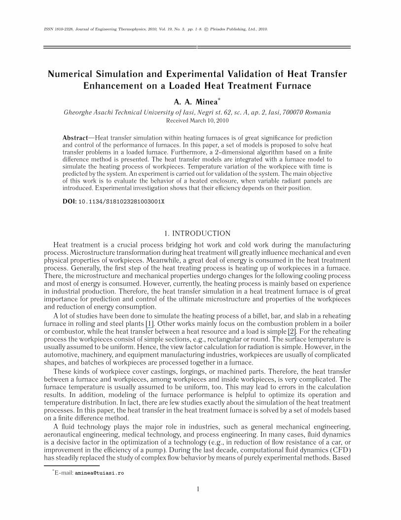
Fig. 1. Panels geometry.

on these simulations it is possible to study three-dimensional flow behavior together with processes suchas combustion, radiation, and environmental emissions. The simulations allow new insights to be gainedwithout resorting to expensive experimental methods right at the beginning of the design process.

Simulation of heat transfer in a heating furnace is of great importance for the prediction and controlof the ultimate microstructure and properties of workpieces.

Furnaces are used in a wide variety of applications including power plants, nuclear reactors, refriger-ation, and other heating systems, automotive industries, heat recovery systems, chemical processing,and food industries [3]. Besides the performance of the furnace being improved, the heat transferenhancement enables the exterior size of the furnace to be considerably decreased.

In this paper, simplified models based on simulation [4] and experimental methods are proposed tocalculate the radiation and convection heat transfer in heating processes. The simulation investigationswere done to understand a forced laminar fluid flow in the furnace walls boundary layer when panels areintroduced. These panels, showed in Fig. 1, were used in simulation and an experiment is carried out forvalidation of the system.

2. REAL LIFE EXAMPLE

2.1. Simulation

A very popular approach to modeling heat transfer is fixed grid enthalpy in which fluid and solid zonesare not treated separately, but a common grid is used in the entire region. For solving the heat transferproblem, we have chosen simulation of radiation and convection in a closed domain.

An important first step for establishing the model accuracy was to identify the boundary conditionsand the properties of materials involved in the process. All the fluid properties were assessed at the meantemperature of the fluids (average of inlet and outlet temperatures) [5]. The models used in the simulationare represented in Table 1. The solver controls are provided in Table 2.

The above formulation was used to build a model using a FLUENT commercial CFD code, whichis the most performing program of numerical simulation of the flows and CFD software is consideredto be an appropriate solver for analysis and simulation of fluids dynamics, used for complex flows inincompressible regimes (subsonic), easily compressible (transonic), and strongly compressible (super-sonic and hypersonic). It is due to an impressive gamma of options combined with numeric algorithmsfor stability and rapid convergence and offers optimum and accurate efficiency for a varied flows domain.The multitude of physical models permit the simulation of laminar and turbulent flows, heat transfer,chemical reactions, multiphase flows, and other phenomena, with a total flexibility toward digitizationscale also offering the possibility of its adjustment based on an intermediary solution.

A classical geometry was simulated to study the effect of heat chamber geometry on heat transferrate. The final default interior temperature was also compared and favorable agreement was observed.

JOURNAL OF ENGINEERING THERMOPHYSICS Vol. 19 No. 3 2010

NUMERICAL SIMULATION AND EXPERIMENTAL VALIDATION 3

Table 1. Simulation models

Model Settings

Space 2D

Time Unsteady, 1st-order implicit

Viscous Laminar

Heat transfer Enabled

Radiation Discrete ordinate model

Table 2. Experiment programming

Factor Panels’ adjustment distance x, mm

Basic Level 120

Variation interval 20

Superior Level (+1) 200

Inferior Level (−1) 80

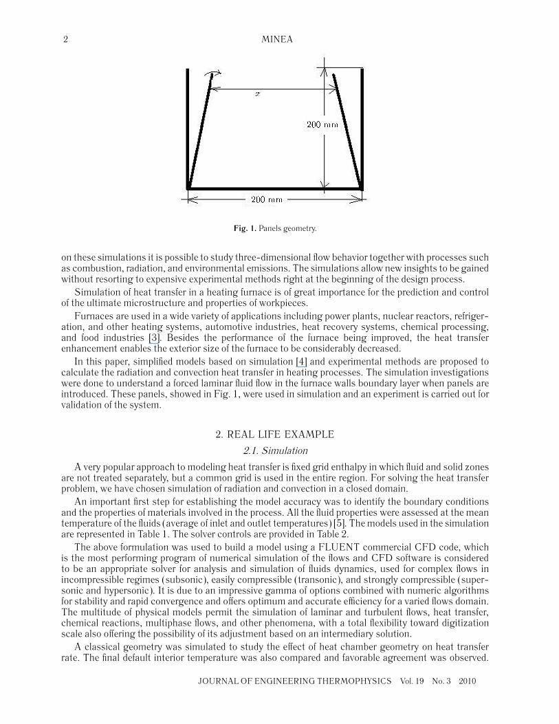
Fig. 2. Configuration of the studied grid.

The models were made on Gambit preprocessor for FLUENT. First of all, we made a base model, grid-independent, and after this, with the help of the journal files from Gambit we obtained all the consideredgeometries. The simulation was in the same conditions for all the models realized and with an iterationof 1200 steps.

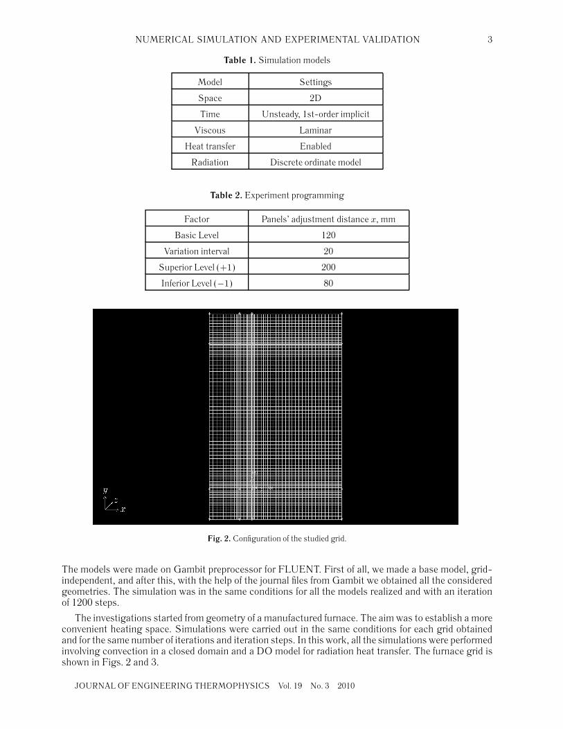
The investigations started from geometry of a manufactured furnace. The aim was to establish a moreconvenient heating space. Simulations were carried out in the same conditions for each grid obtainedand for the same number of iterations and iteration steps. In this work, all the simulations were performedinvolving convection in a closed domain and a DO model for radiation heat transfer. The furnace grid isshown in Figs. 2 and 3.

JOURNAL OF ENGINEERING THERMOPHYSICS Vol. 19 No. 3 2010

4 MINEA

Fig. 3. Configuration of the studied grid with panels inside.

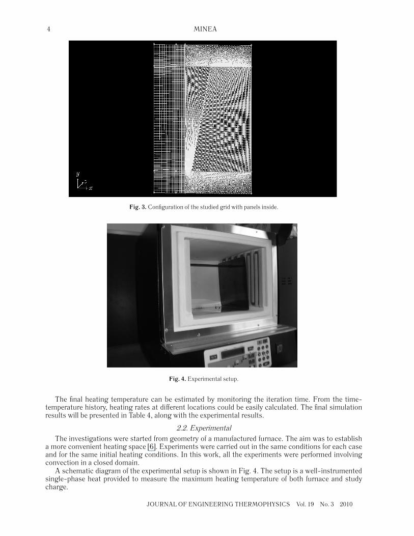
Fig. 4. Experimental setup.

The final heating temperature can be estimated by monitoring the iteration time. From the time-temperature history, heating rates at different locations could be easily calculated. The final simulationresults will be presented in Table 4, along with the experimental results.

2.2. ExperimentalThe investigations were started from geometry of a manufactured furnace. The aim was to establish

a more convenient heating space [6]. Experiments were carried out in the same conditions for each caseand for the same initial heating conditions. In this work, all the experiments were performed involvingconvection in a closed domain.

A schematic diagram of the experimental setup is shown in Fig. 4. The setup is a well-instrumentedsingle-phase heat provided to measure the maximum heating temperature of both furnace and studycharge.

JOURNAL OF ENGINEERING THERMOPHYSICS Vol. 19 No. 3 2010

NUMERICAL SIMULATION AND EXPERIMENTAL VALIDATION 5

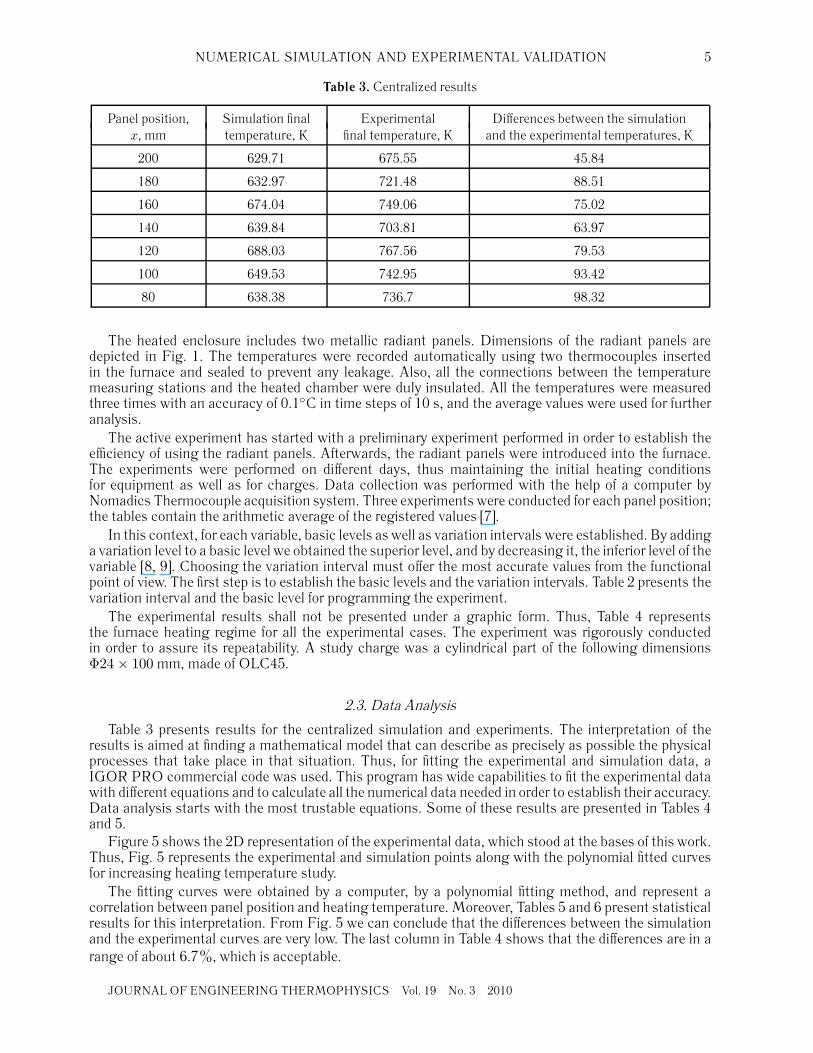
Table 3. Centralized results

Panel position, Simulation final Experimental Differences between the simulationx, mm temperature, K final temperature, K and the experimental temperatures, K

200 629.71 675.55 45.84

180 632.97 721.48 88.51

160 674.04 749.06 75.02

140 639.84 703.81 63.97

120 688.03 767.56 79.53

100 649.53 742.95 93.42

80 638.38 736.7 98.32

The heated enclosure includes two metallic radiant panels. Dimensions of the radiant panels aredepicted in Fig. 1. The temperatures were recorded automatically using two thermocouples insertedin the furnace and sealed to prevent any leakage. Also, all the connections between the temperaturemeasuring stations and the heated chamber were duly insulated. All the temperatures were measuredthree times with an accuracy of 0.1◦C in time steps of 10 s, and the average values were used for furtheranalysis.

The active experiment has started with a preliminary experiment performed in order to establish theefficiency of using the radiant panels. Afterwards, the radiant panels were introduced into the furnace.The experiments were performed on different days, thus maintaining the initial heating conditionsfor equipment as well as for charges. Data collection was performed with the help of a computer byNomadics Thermocouple acquisition system. Three experiments were conducted for each panel position;the tables contain the arithmetic average of the registered values [7].

In this context, for each variable, basic levels as well as variation intervals were established. By addinga variation level to a basic level we obtained the superior level, and by decreasing it, the inferior level of thevariable [8, 9]. Choosing the variation interval must offer the most accurate values from the functionalpoint of view. The first step is to establish the basic levels and the variation intervals. Table 2 presents thevariation interval and the basic level for programming the experiment.

The experimental results shall not be presented under a graphic form. Thus, Table 4 representsthe furnace heating regime for all the experimental cases. The experiment was rigorously conductedin order to assure its repeatability. A study charge was a cylindrical part of the following dimensionsΦ24 × 100 mm, made of OLC45.

2.3. Data Analysis

Table 3 presents results for the centralized simulation and experiments. The interpretation of theresults is aimed at finding a mathematical model that can describe as precisely as possible the physicalprocesses that take place in that situation. Thus, for fitting the experimental and simulation data, aIGOR PRO commercial code was used. This program has wide capabilities to fit the experimental datawith different equations and to calculate all the numerical data needed in order to establish their accuracy.Data analysis starts with the most trustable equations. Some of these results are presented in Tables 4and 5.

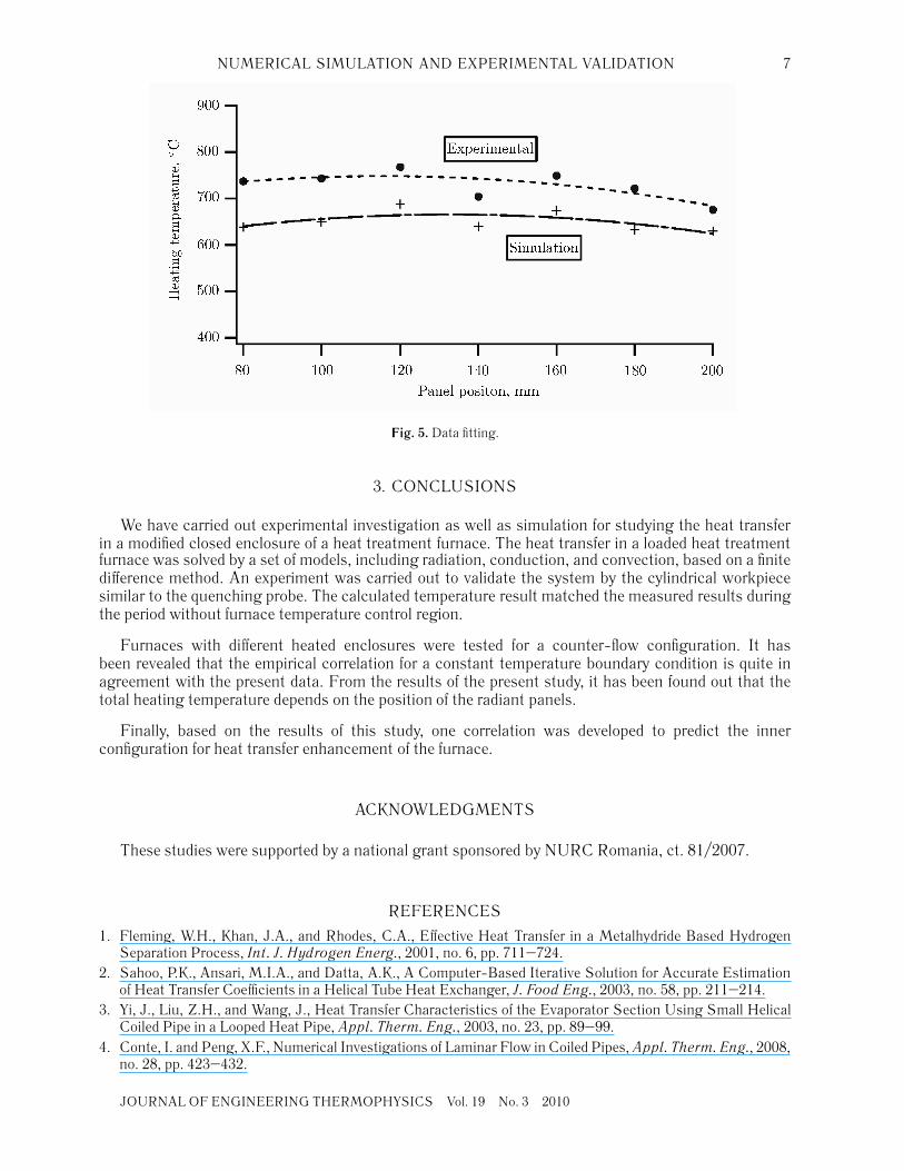
Figure 5 shows the 2D representation of the experimental data, which stood at the bases of this work.Thus, Fig. 5 represents the experimental and simulation points along with the polynomial fitted curvesfor increasing heating temperature study.

The fitting curves were obtained by a computer, by a polynomial fitting method, and represent acorrelation between panel position and heating temperature. Moreover, Tables 5 and 6 present statisticalresults for this interpretation. From Fig. 5 we can conclude that the differences between the simulationand the experimental curves are very low. The last column in Table 4 shows that the differences are in arange of about 6.7%, which is acceptable.

JOURNAL OF ENGINEERING THERMOPHYSICS Vol. 19 No. 3 2010

6 MINEA

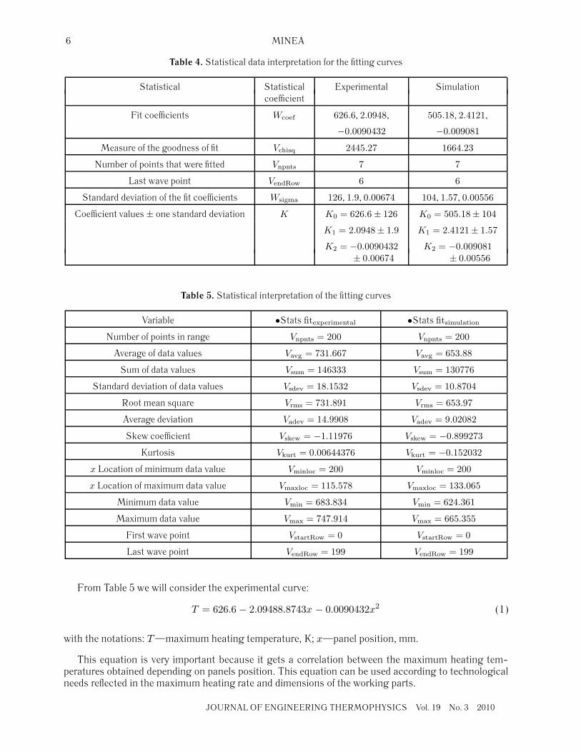
Table 4. Statistical data interpretation for the fitting curves

Statistical Statistical Experimental Simulationcoefficient

Fit coefficients Wcoef 626.6, 2.0948, 505.18, 2.4121,

−0.0090432 −0.009081

Measure of the goodness of fit Vchisq 2445.27 1664.23

Number of points that were fitted Vnpnts 7 7

Last wave point VendRow 6 6

Standard deviation of the fit coefficients Wsigma 126, 1.9, 0.00674 104, 1.57, 0.00556

Coefficient values ± one standard deviation K K0 = 626.6 ± 126 K0 = 505.18± 104

K1 = 2.0948± 1.9 K1 = 2.4121± 1.57

K2 = −0.0090432 K2 = −0.009081± 0.00674 ± 0.00556

Table 5. Statistical interpretation of the fitting curves

Variable •Stats fitexperimental •Stats fitsimulation

Number of points in range Vnpnts = 200 Vnpnts = 200

Average of data values Vavg = 731.667 Vavg = 653.88

Sum of data values Vsum = 146333 Vsum = 130776

Standard deviation of data values Vsdev = 18.1532 Vsdev = 10.8704

Root mean square Vrms = 731.891 Vrms = 653.97

Average deviation Vadev = 14.9908 Vadev = 9.02082

Skew coefficient Vskew = −1.11976 Vskew = −0.899273

Kurtosis Vkurt = 0.00644376 Vkurt = −0.152032

x Location of minimum data value Vminloc = 200 Vminloc = 200

x Location of maximum data value Vmaxloc = 115.578 Vmaxloc = 133.065

Minimum data value Vmin = 683.834 Vmin = 624.361

Maximum data value Vmax = 747.914 Vmax = 665.355

First wave point VstartRow = 0 VstartRow = 0

Last wave point VendRow = 199 VendRow = 199

From Table 5 we will consider the experimental curve:

T = 626.6 − 2.09488.8743x − 0.0090432x2 (1)

with the notations: T —maximum heating temperature, K; x—panel position, mm.

This equation is very important because it gets a correlation between the maximum heating tem-peratures obtained depending on panels position. This equation can be used according to technologicalneeds reflected in the maximum heating rate and dimensions of the working parts.

JOURNAL OF ENGINEERING THERMOPHYSICS Vol. 19 No. 3 2010

NUMERICAL SIMULATION AND EXPERIMENTAL VALIDATION 7

Fig. 5. Data fitting.

3. CONCLUSIONS

We have carried out experimental investigation as well as simulation for studying the heat transferin a modified closed enclosure of a heat treatment furnace. The heat transfer in a loaded heat treatmentfurnace was solved by a set of models, including radiation, conduction, and convection, based on a finitedifference method. An experiment was carried out to validate the system by the cylindrical workpiecesimilar to the quenching probe. The calculated temperature result matched the measured results duringthe period without furnace temperature control region.

Furnaces with different heated enclosures were tested for a counter-flow configuration. It hasbeen revealed that the empirical correlation for a constant temperature boundary condition is quite inagreement with the present data. From the results of the present study, it has been found out that thetotal heating temperature depends on the position of the radiant panels.

Finally, based on the results of this study, one correlation was developed to predict the innerconfiguration for heat transfer enhancement of the furnace.

ACKNOWLEDGMENTS

These studies were supported by a national grant sponsored by NURC Romania, ct. 81/2007.

REFERENCES

1. Fleming, W.H., Khan, J.A., and Rhodes, C.A., Effective Heat Transfer in a Metalhydride Based HydrogenSeparation Process, Int. J. Hydrogen Energ., 2001, no. 6, pp. 711–724.

2. Sahoo, P.K., Ansari, M.I.A., and Datta, A.K., A Computer-Based Iterative Solution for Accurate Estimationof Heat Transfer Coefficients in a Helical Tube Heat Exchanger, J. Food Eng., 2003, no. 58, pp. 211–214.

3. Yi, J., Liu, Z.H., and Wang, J., Heat Transfer Characteristics of the Evaporator Section Using Small HelicalCoiled Pipe in a Looped Heat Pipe, Appl. Therm. Eng., 2003, no. 23, pp. 89–99.

4. Conte, I. and Peng, X.F., Numerical Investigations of Laminar Flow in Coiled Pipes, Appl. Therm. Eng., 2008,no. 28, pp. 423–432.

JOURNAL OF ENGINEERING THERMOPHYSICS Vol. 19 No. 3 2010

8 MINEA

5. White, F.M., Heat Transfer, New York: Addison-Wesley, 1984.6. Chui, E.H., Raithby, G.D., and Hughes, P.M., Prediction of Radiative Heat Transfer in Enclosures by the Finite

Volume Method, J. Thermophys. Heat Transfer, 1992, no. 92.7. Kang, J., Rong, Y.K., and Wang, W., Numerical Simulation of Heat Transfer in Loaded Heat Treatment

Furnaces, J. Phys. IV France, 2004, pp. 545–553;http://publications.edpsciences.org/articles/jp4/pdf/2004/08/Jp4120063.pdf.

8. Ful-Chiang, W., Simultaneous Optimization of Robust Design with Quantitative and Ordinal Data, Int. J.Industrial Eng., Th., Appl. Pract., 2008, vol. 15, no. 2, pp. 231–238.

9. Guneri, A.F. and Gumus, A.T., Artificial Neural Networks for Finite Capacity Scheduling: A ComparativeStudy, Int. J. Industrial Eng., Th., Appl. Pract., 2008, vol. 15, no. 4, pp. 349–359.

JOURNAL OF ENGINEERING THERMOPHYSICS Vol. 19 No. 3 2010