
Numerical Optimization Applied to Space-Related Problems
46
Numerical Optimization Applied to Space-Related Problems Robert J. Vanderbei 2016 November 18 Center for Applied Math, Cornell University http://www.princeton.edu/∼rvdb
-
Upload
khangminh22 -
Category
Documents
-
view
2 -
download
0
Transcript of Numerical Optimization Applied to Space-Related Problems

Numerical Optimization Applied to Space-Related Problems
Robert J. Vanderbei
2016 November 18
Center for Applied Math, Cornell University
http://www.princeton.edu/∼rvdb

The Plan...
Planet Finding via High-Contrast Imaging
Fast-Fourier Optimization — Sparsifying the Constraint Matrix
New Solutions to the n-Body Problem
0

The Plan...
Planet Finding via High-Contrast Imaging
Fast-Fourier Optimization — Sparsifying the Constraint Matrix
New Solutions to the n-Body Problem
1

2
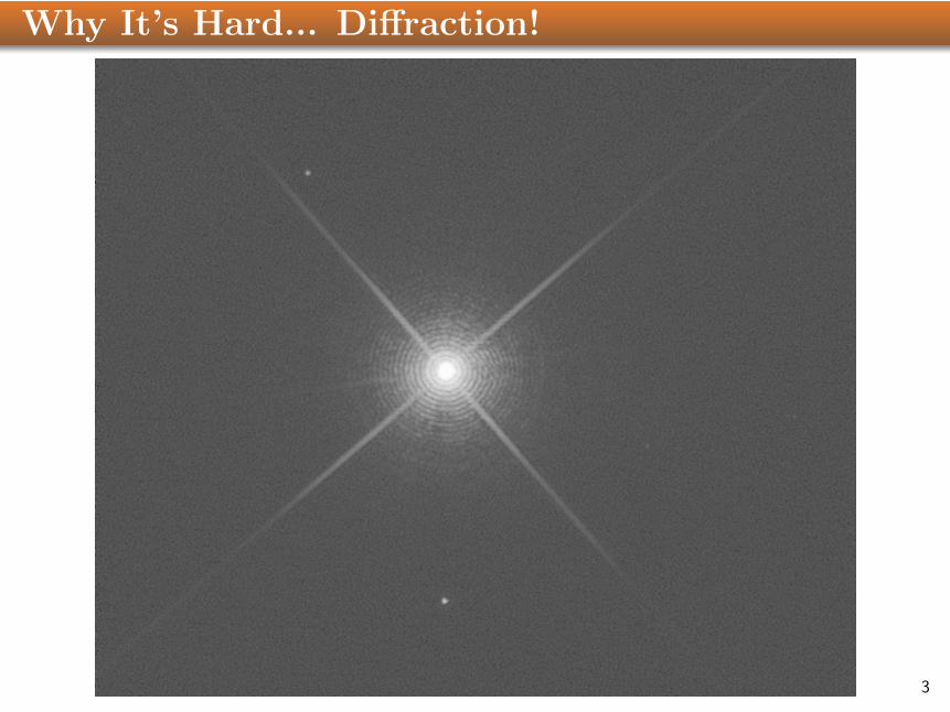
Why It’s Hard... Diffraction!
3
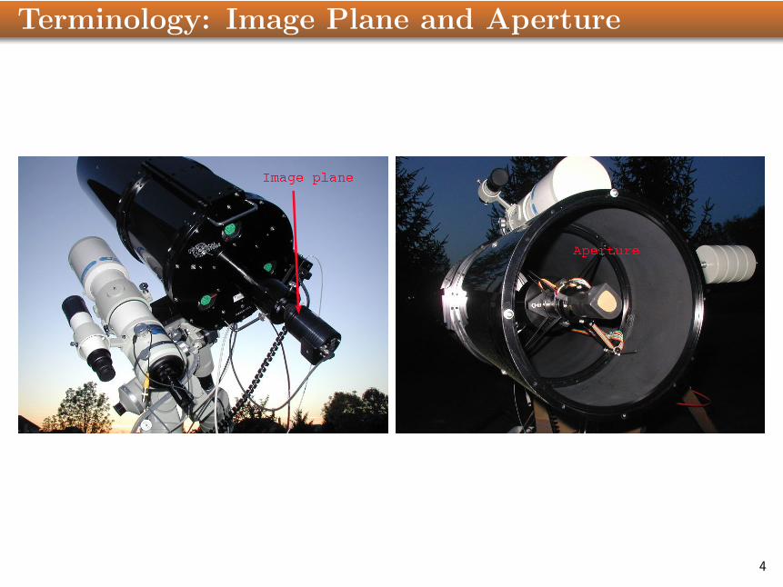
Terminology: Image Plane and Aperture
4
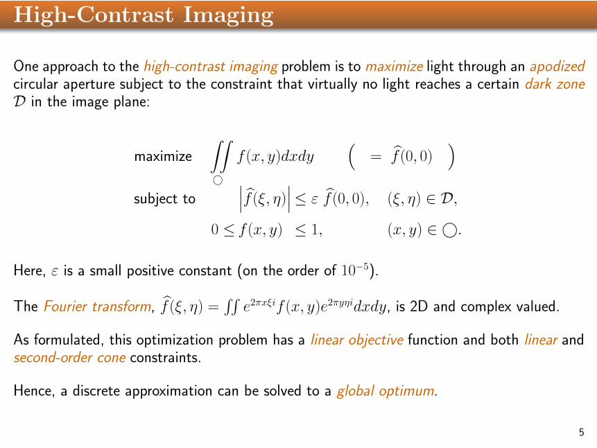
High-Contrast Imaging
One approach to the high-contrast imaging problem is to maximize light through an apodizedcircular aperture subject to the constraint that virtually no light reaches a certain dark zoneD in the image plane:
maximize
∫∫©
f (x, y)dxdy(
= f (0, 0))
subject to∣∣∣f (ξ, η)
∣∣∣≤ ε f (0, 0), (ξ, η) ∈ D,
0 ≤ f (x, y) ≤ 1, (x, y) ∈ ©.
Here, ε is a small positive constant (on the order of 10−5).
The Fourier transform, f (ξ, η) =∫∫e2πxξif (x, y)e2πyηidxdy, is 2D and complex valued.
As formulated, this optimization problem has a linear objective function and both linear andsecond-order cone constraints.
Hence, a discrete approximation can be solved to a global optimum.
5
Misconceptions
AM: The Fourier transform is well understood. The best algorithm for computing it is thefast Fourier transform. Excellent codes are available, such as fftw. Just call one ofthese state-of-the-art codes. There is nothing new to be done here.
Wrong! Efficient algorithms for linear programming require more than an or-acle that computes constraint function values. They also need gradients. Towork with the full Jacobian matrix of the Fourier transform is to loose all of thecomputational efficiency of the fast Fourier transform.
OR: The range of problems that fit the Fourier Optimization paradigm is very limited.There might be some new research, but its applications are few.
Wrong! Almost every problem in electrical engineering involves Fourier trans-forms. And the idea can be extended beyond Fourier transforms. The list ofapplications is yuge!
6
Misconceptions
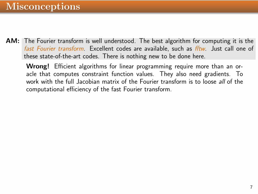
AM: The Fourier transform is well understood. The best algorithm for computing it is thefast Fourier transform. Excellent codes are available, such as fftw. Just call one ofthese state-of-the-art codes. There is nothing new to be done here.
Wrong! Efficient algorithms for linear programming require more than an or-acle that computes constraint function values. They also need gradients. Towork with the full Jacobian matrix of the Fourier transform is to loose all of thecomputational efficiency of the fast Fourier transform.
OR: The range of problems that fit the Fourier Optimization paradigm is very limited.There might be some new research, but its applications are few.
Wrong! Almost every problem in electrical engineering involves Fourier trans-forms. And the idea can be extended beyond Fourier transforms. The list ofapplications is yuge!
7
Misconceptions
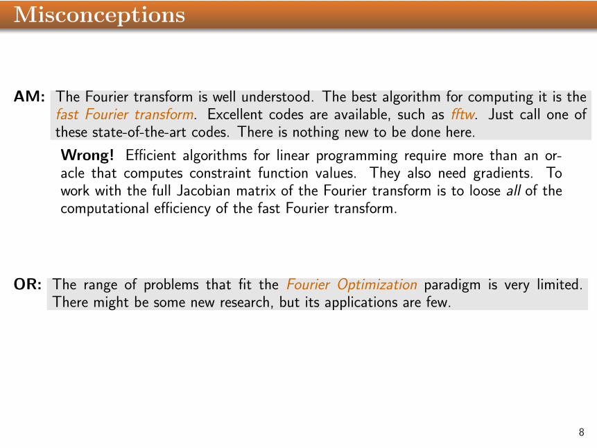
AM: The Fourier transform is well understood. The best algorithm for computing it is thefast Fourier transform. Excellent codes are available, such as fftw. Just call one ofthese state-of-the-art codes. There is nothing new to be done here.
Wrong! Efficient algorithms for linear programming require more than an or-acle that computes constraint function values. They also need gradients. Towork with the full Jacobian matrix of the Fourier transform is to loose all of thecomputational efficiency of the fast Fourier transform.
OR: The range of problems that fit the Fourier Optimization paradigm is very limited.There might be some new research, but its applications are few.
Wrong! Almost every problem in electrical engineering involves Fourier trans-forms. And the idea can be extended beyond Fourier transforms. The list ofapplications is yuge!
8
Misconceptions
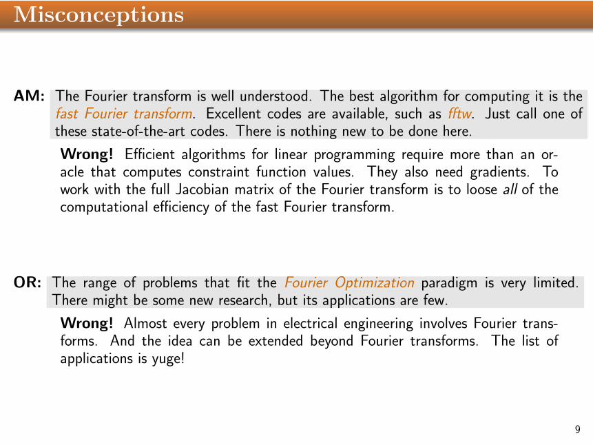
AM: The Fourier transform is well understood. The best algorithm for computing it is thefast Fourier transform. Excellent codes are available, such as fftw. Just call one ofthese state-of-the-art codes. There is nothing new to be done here.
Wrong! Efficient algorithms for linear programming require more than an or-acle that computes constraint function values. They also need gradients. Towork with the full Jacobian matrix of the Fourier transform is to loose all of thecomputational efficiency of the fast Fourier transform.
OR: The range of problems that fit the Fourier Optimization paradigm is very limited.There might be some new research, but its applications are few.
Wrong! Almost every problem in electrical engineering involves Fourier trans-forms. And the idea can be extended beyond Fourier transforms. The list ofapplications is yuge!
9
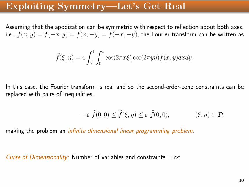
Exploiting Symmetry—Let’s Get Real
Assuming that the apodization can be symmetric with respect to reflection about both axes,i.e., f (x, y) = f (−x, y) = f (x,−y) = f (−x,−y), the Fourier transform can be written as
f (ξ, η) = 4
∫ 1
0
∫ 1
0
cos(2πxξ) cos(2πyη)f (x, y)dxdy.
In this case, the Fourier transform is real and so the second-order-cone constraints can bereplaced with pairs of inequalities,
− ε f (0, 0) ≤ f (ξ, η) ≤ ε f (0, 0), (ξ, η) ∈ D,
making the problem an infinite dimensional linear programming problem.
Curse of Dimensionality: Number of variables and constraints =∞
10
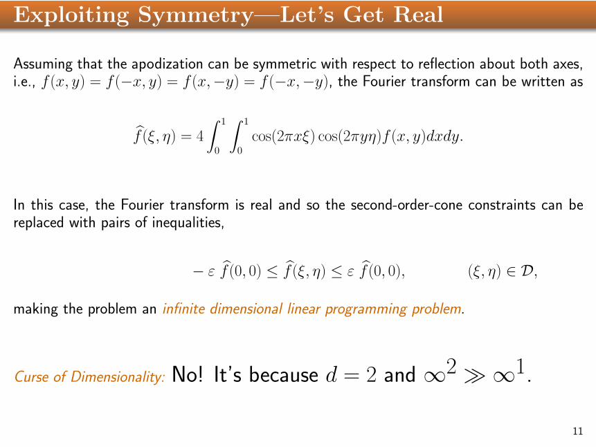
Exploiting Symmetry—Let’s Get Real
Assuming that the apodization can be symmetric with respect to reflection about both axes,i.e., f (x, y) = f (−x, y) = f (x,−y) = f (−x,−y), the Fourier transform can be written as
f (ξ, η) = 4
∫ 1
0
∫ 1
0
cos(2πxξ) cos(2πyη)f (x, y)dxdy.
In this case, the Fourier transform is real and so the second-order-cone constraints can bereplaced with pairs of inequalities,
− ε f (0, 0) ≤ f (ξ, η) ≤ ε f (0, 0), (ξ, η) ∈ D,
making the problem an infinite dimensional linear programming problem.
Curse of Dimensionality: No! It’s because d = 2 and ∞2�∞1.
11
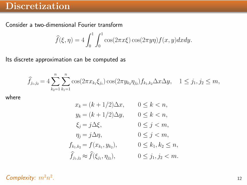
Discretization
Consider a two-dimensional Fourier transform
f (ξ, η) = 4
∫ 1
0
∫ 1
0
cos(2πxξ) cos(2πyη)f (x, y)dxdy.
Its discrete approximation can be computed as
fj1,j2 = 4n∑
k2=1
n∑k1=1
cos(2πxk1ξj1) cos(2πyk2ηj2)fk1,k2∆x∆y, 1 ≤ j1, j2 ≤ m,
wherexk = (k + 1/2)∆x, 0 ≤ k < n,
yk = (k + 1/2)∆y, 0 ≤ k < n,
ξj = j∆ξ, 0 ≤ j < m,
ηj = j∆η, 0 ≤ j < m,
fk1,k2 = f (xk1, yk2), 0 ≤ k1, k2 ≤ n,
fj1,j2 ≈ f (ξj1, ηj2), 0 ≤ j1, j2 < m.
Complexity: m2n2. 12
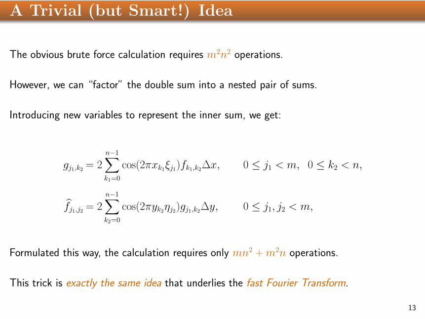
A Trivial (but Smart!) Idea
The obvious brute force calculation requires m2n2 operations.
However, we can “factor” the double sum into a nested pair of sums.
Introducing new variables to represent the inner sum, we get:
gj1,k2 = 2n−1∑k1=0
cos(2πxk1ξj1)fk1,k2∆x, 0 ≤ j1 < m, 0 ≤ k2 < n,
fj1,j2 = 2n−1∑k2=0
cos(2πyk2ηj2)gj1,k2∆y, 0 ≤ j1, j2 < m,
Formulated this way, the calculation requires only mn2 + m2n operations.
This trick is exactly the same idea that underlies the fast Fourier Transform.
13
Brute Force vs Clever Approach
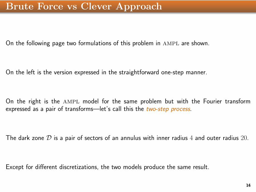
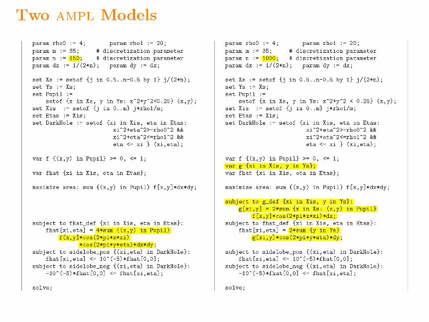
On the following page two formulations of this problem in ampl are shown.
On the left is the version expressed in the straightforward one-step manner.
On the right is the ampl model for the same problem but with the Fourier transformexpressed as a pair of transforms—let’s call this the two-step process.
The dark zone D is a pair of sectors of an annulus with inner radius 4 and outer radius 20.
Except for different discretizations, the two models produce the same result.
1415
15
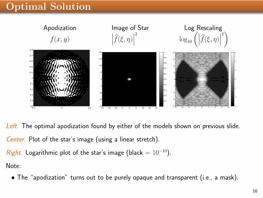
Optimal Solution
Apodization Image of Star Log Rescaling
f (x, y)∣∣∣f (ξ, η)
∣∣∣2 log10
(∣∣∣f (ξ, η)∣∣∣2)
−0.5 0 0.5
−0.5
−0.4
−0.3
−0.2
−0.1
0
0.1
0.2
0.3
0.4
0.5
−20 −15 −10 −5 0 5 10 15 20
−20
−15
−10
−5
0
5
10
15
20
0.1
0.2
0.3
0.4
0.5
0.6
0.7
0.8
0.9
1
-20 -15 -10 -5 0 5 10 15 20
-20
-15
-10
-5
0
5
10
15
20 -12
-10
-8
-6
-4
-2
0
Left. The optimal apodization found by either of the models shown on previous slide.
Center. Plot of the star’s image (using a linear stretch).
Right. Logarithmic plot of the star’s image (black = 10−10).
Note:
• The “apodization” turns out to be purely opaque and transparent (i.e., a mask).
16
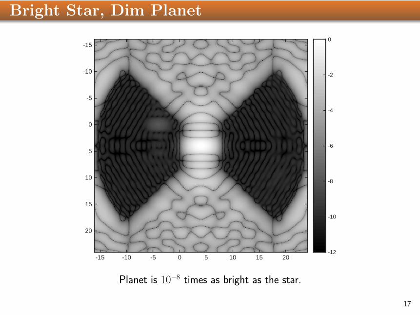
Bright Star, Dim Planet
-15 -10 -5 0 5 10 15 20
-15
-10
-5
0
5
10
15
20
-12
-10
-8
-6
-4
-2
0
Planet is 10−8 times as bright as the star.
17
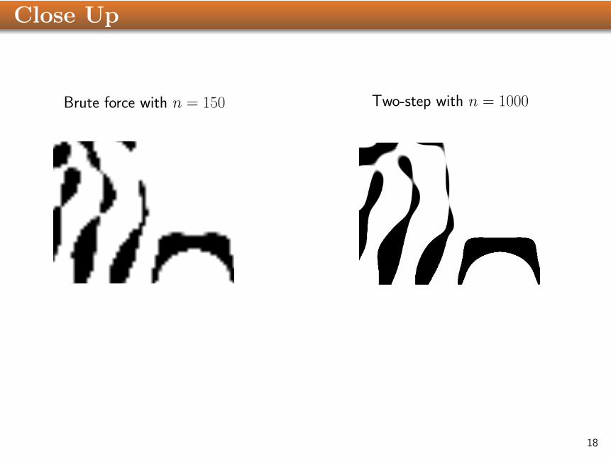
Close Up
Brute force with n = 150
−0.5 0 0.5
−0.5
−0.4
−0.3
−0.2
−0.1
0
0.1
0.2
0.3
0.4
0.5
Two-step with n = 1000
−0.5 0 0.5
−0.5
−0.4
−0.3
−0.2
−0.1
0
0.1
0.2
0.3
0.4
0.5
18
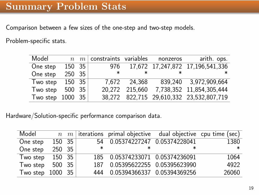
Summary Problem Stats
Comparison between a few sizes of the one-step and two-step models.
Problem-specific stats.
Model n m constraints variables nonzeros arith. ops.One step 150 35 976 17,672 17,247,872 17,196,541,336One step 250 35 * * * *Two step 150 35 7,672 24,368 839,240 3,972,909,664Two step 500 35 20,272 215,660 7,738,352 11,854,305,444Two step 1000 35 38,272 822,715 29,610,332 23,532,807,719
Hardware/Solution-specific performance comparison data.
Model n m iterations primal objective dual objective cpu time (sec)One step 150 35 54 0.05374227247 0.05374228041 1380One step 250 35 * * * *Two step 150 35 185 0.05374233071 0.05374236091 1064Two step 500 35 187 0.05395622255 0.05395623990 4922Two step 1000 35 444 0.05394366337 0.05394369256 26060
19
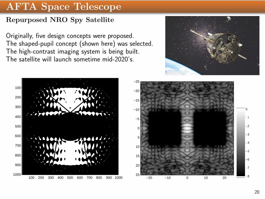
AFTA Space TelescopeRepurposed NRO Spy Satellite
Originally, five design concepts were proposed.The shaped-pupil concept (shown here) was selected.The high-contrast imaging system is being built.The satellite will launch sometime mid-2020’s.
100 200 300 400 500 600 700 800 900 1000
100
200
300
400
500
600
700
800
900
1000−20 −10 0 10 20
−25
−20
−15
−10
−5
0
5
10
15
20
25
20

The Plan...
Planet Finding via High-Contrast Imaging
Fast-Fourier Optimization — Sparsifying the Constraint Matrix
New Solutions to the n-Body Problem
21
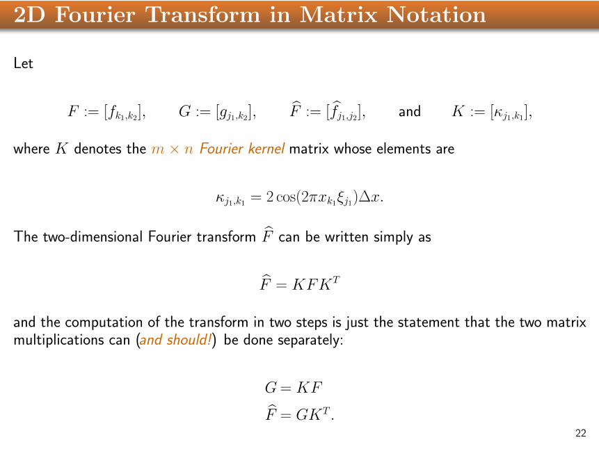
2D Fourier Transform in Matrix Notation
Let
F := [fk1,k2], G := [gj1,k2], F := [fj1,j2], and K := [κj1,k1],
where K denotes the m× n Fourier kernel matrix whose elements are
κj1,k1 = 2 cos(2πxk1ξj1)∆x.
The two-dimensional Fourier transform F can be written simply as
F = KFKT
and the computation of the transform in two steps is just the statement that the two matrixmultiplications can (and should!) be done separately:
G= KF
F = GKT .22
Clever Idea = Matrix Sparsification
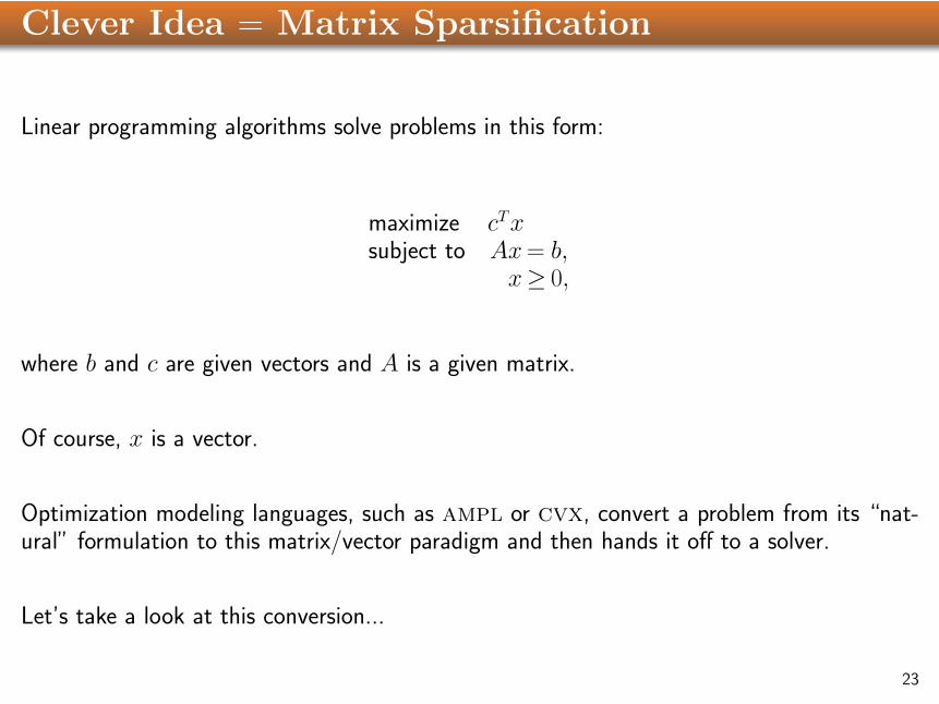
Linear programming algorithms solve problems in this form:
maximize cTxsubject to Ax= b,
x≥ 0,
where b and c are given vectors and A is a given matrix.
Of course, x is a vector.
Optimization modeling languages, such as ampl or cvx, convert a problem from its “nat-ural” formulation to this matrix/vector paradigm and then hands it off to a solver.
Let’s take a look at this conversion...
23
Vectorizing...
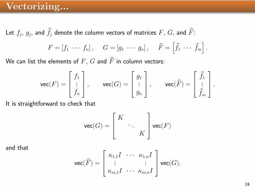
Let fj, gj, and fj denote the column vectors of matrices F , G, and F :
F = [f1 · · · fn] , G = [g1 · · · gn] , F =[f1 · · · fm
].
We can list the elements of F , G and F in column vectors:
vec(F ) =
f1...fn
, vec(G) =
g1...gn
, vec(F ) =
f1...
fm
.It is straightforward to check that
vec(G) =
K . . .K
vec(F )
and that
vec(F ) =
κ1,1I · · · κ1,nI... ...
κm,1I · · · κm,nI
vec(G).
24

One-Step Method:κ1,1K · · · κ1,nK −I
... ... . . .κm,1K · · · κm,nK −I
... ...
f1...fn
f1...
fm
=
0...0...
The big left block is a dense m2 × n2 matrix.——————————————————————————————————Two-Step Method:
K −I. . . . . .
K −Iκ1,1I · · · κ1,nI −I
... ... . . .κm,1I · · · κm,nI −I
... ... ...
f1...fn
g1...gn
f1...
fm
=
0...00...0...
The big upper-left block is a sparse block-diagonal mn× n2 matrix with mn2 nonzeros.
The middle block is an m× n matrix of sub-blocks that are each m×m diagonal matrices.Hence, it is very sparse, containing only m2n nonzeros. 25
References
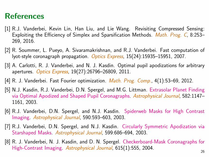
[1] R.J. Vanderbei, Kevin Lin, Han Liu, and Lie Wang. Revisiting Compressed Sensing:Exploiting the Efficiency of Simplex and Sparsification Methods. Math. Prog. C, 8:253–269, 2016.
[2] R. Soummer, L. Pueyo, A. Sivaramakrishnan, and R.J. Vanderbei. Fast computation oflyot-style coronagraph propagation. Optics Express, 15(24):15935–15951, 2007.
[3] A. Carlotti, R. J. Vanderbei, and N. J. Kasdin. Optimal pupil apodizations for arbitraryapertures. Optics Express, 19(27):26796–26809, 2011.
[4] R. J. Vanderbei. Fast Fourier optimization. Math. Prog. Comp., 4(1):53–69, 2012.
[5] N.J. Kasdin, R.J. Vanderbei, D.N. Spergel, and M.G. Littman. Extrasolar Planet Findingvia Optimal Apodized and Shaped Pupil Coronagraphs. Astrophysical Journal, 582:1147–1161, 2003.
[6] R.J. Vanderbei, D.N. Spergel, and N.J. Kasdin. Spiderweb Masks for High ContrastImaging. Astrophysical Journal, 590:593–603, 2003.
[7] R.J. Vanderbei, D.N. Spergel, and N.J. Kasdin. Circularly Symmetric Apodization viaStarshaped Masks. Astrophysical Journal, 599:686–694, 2003.
[8] R. J. Vanderbei, N. J. Kasdin, and D. N. Spergel. Checkerboard-Mask Coronagraphs forHigh-Contrast Imaging. Astrophysical Journal, 615(1):555, 2004.
26

The Plan...
Planet Finding via High-Contrast Imaging
Fast-Fourier Optimization — Sparsifying the Constraint Matrix
New Solutions to the n-Body Problem
27
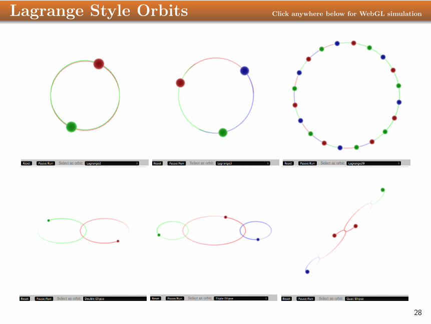
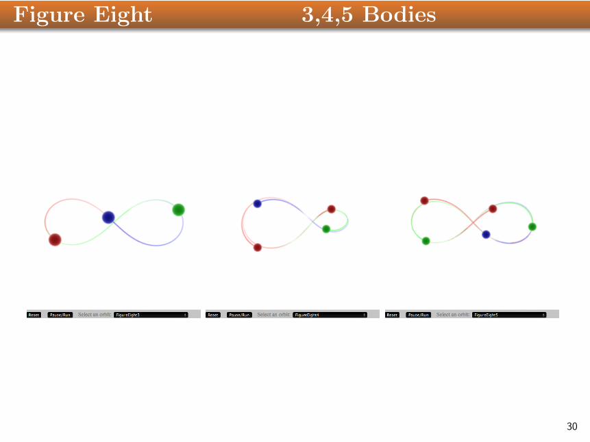
Lagrange Style Orbits Click anywhere below for WebGL simulation
28
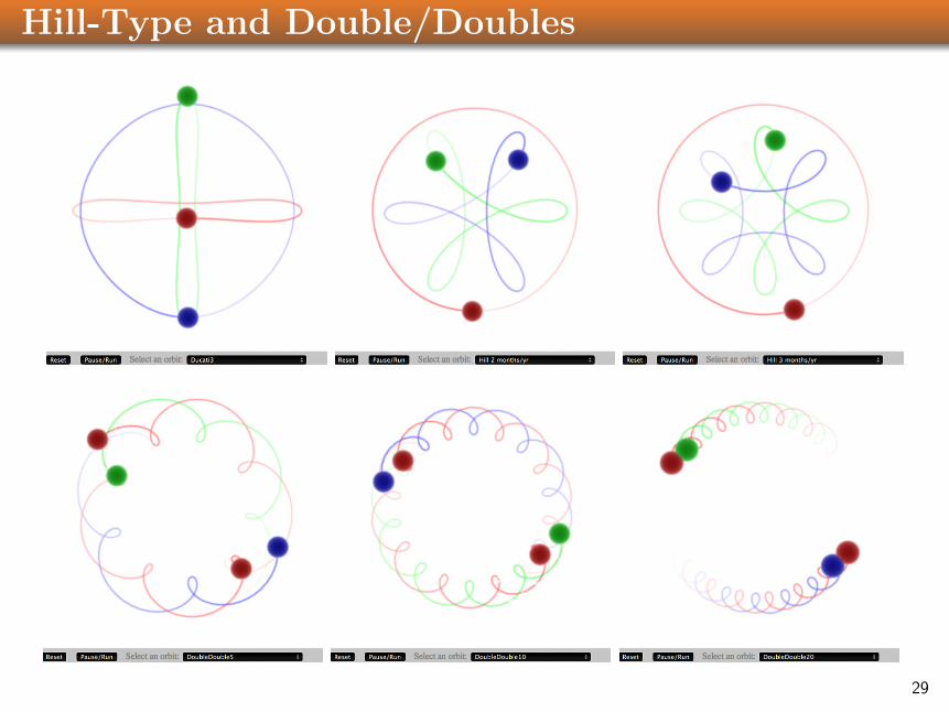
Hill-Type and Double/Doubles
29
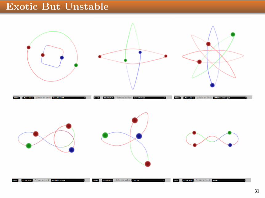
Exotic But Unstable
31
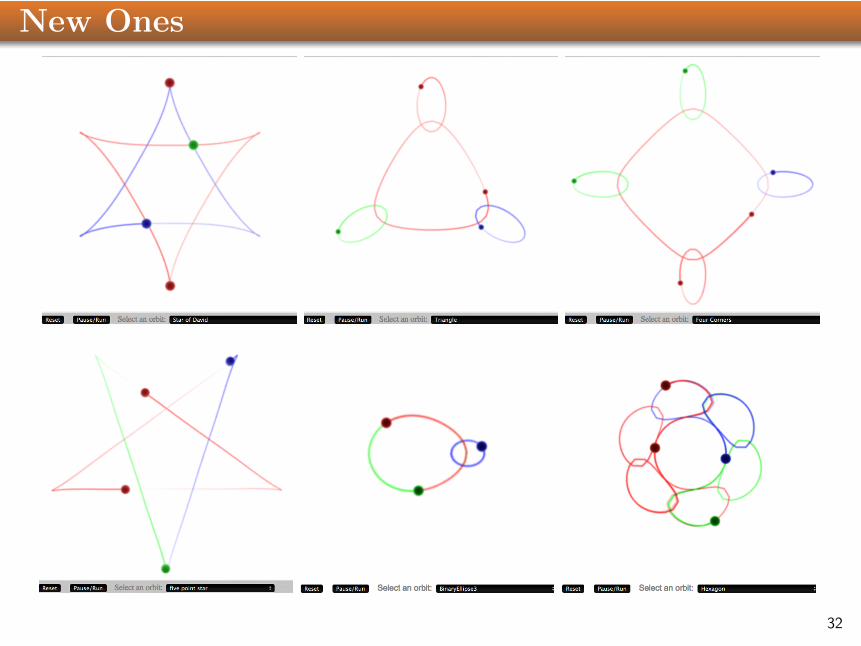
New Ones
32
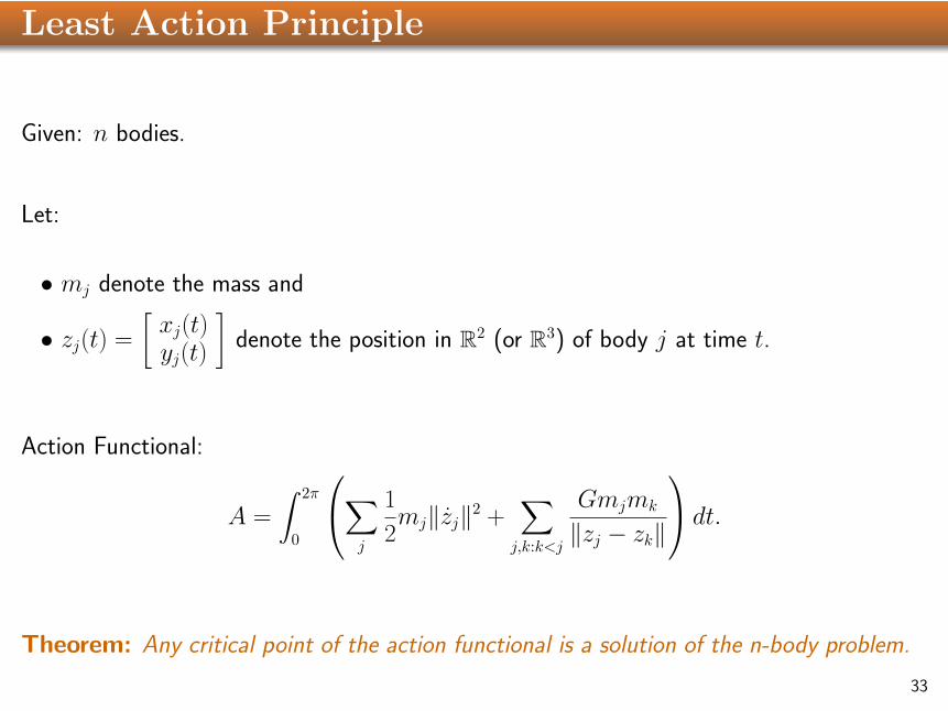
Least Action Principle
Given: n bodies.
Let:
• mj denote the mass and
• zj(t) =
[xj(t)yj(t)
]denote the position in R2 (or R3) of body j at time t.
Action Functional:
A =
∫ 2π
0
∑j
1
2mj‖zj‖2 +
∑j,k:k<j
Gmjmk
‖zj − zk‖
dt.
Theorem: Any critical point of the action functional is a solution of the n-body problem.
33
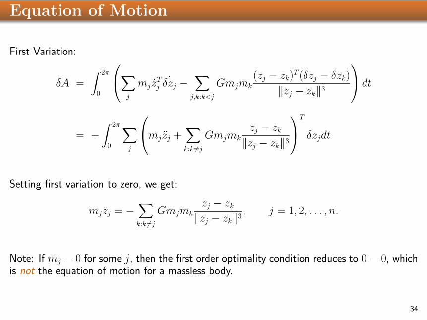
Equation of Motion
First Variation:
δA =
∫ 2π
0
∑j
mjzTj
˙δzj −∑j,k:k<j
Gmjmk
(zj − zk)T (δzj − δzk)‖zj − zk‖3
dt
= −∫ 2π
0
∑j
mjzj +∑k:k 6=j
Gmjmk
zj − zk‖zj − zk‖3
T
δzjdt
Setting first variation to zero, we get:
mjzj = −∑k:k 6=j
Gmjmk
zj − zk‖zj − zk‖3
, j = 1, 2, . . . , n.
Note: If mj = 0 for some j, then the first order optimality condition reduces to 0 = 0, whichis not the equation of motion for a massless body.
34
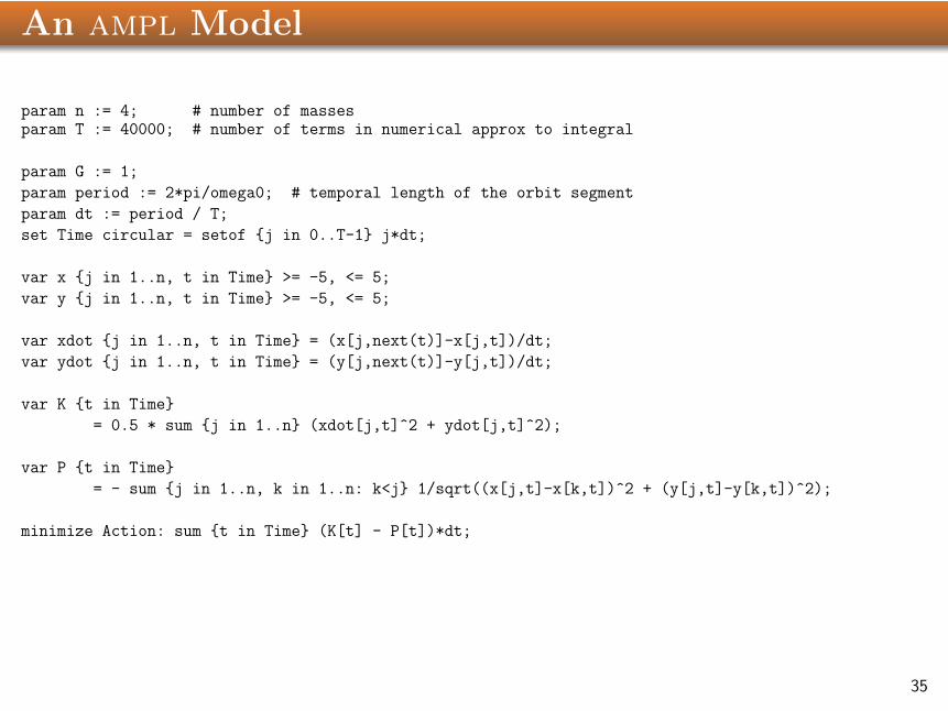
An ampl Model
param n := 4; # number of massesparam T := 40000; # number of terms in numerical approx to integral
param G := 1;
param period := 2*pi/omega0; # temporal length of the orbit segment
param dt := period / T;
set Time circular = setof {j in 0..T-1} j*dt;
var x {j in 1..n, t in Time} >= -5, <= 5;
var y {j in 1..n, t in Time} >= -5, <= 5;
var xdot {j in 1..n, t in Time} = (x[j,next(t)]-x[j,t])/dt;
var ydot {j in 1..n, t in Time} = (y[j,next(t)]-y[j,t])/dt;
var K {t in Time}
= 0.5 * sum {j in 1..n} (xdot[j,t]^2 + ydot[j,t]^2);
var P {t in Time}
= - sum {j in 1..n, k in 1..n: k<j} 1/sqrt((x[j,t]-x[k,t])^2 + (y[j,t]-y[k,t])^2);
minimize Action: sum {t in Time} (K[t] - P[t])*dt;
35

A Double/Double Initialization
param omega0 := 1./2;param omega1 := 1./1;
param phi_p := -pi/2;
param phi_m := pi/2;
param r0 := (G/(2*omega0^2))^(1./3.);
param r1 := (G/(4*omega1^2))^(1./3.);
let {t in Time} x[0,t] := r0*cos(omega0*t) + r1*sin(-omega1*t + phi_p);
let {t in Time} y[0,t] := r0*sin(omega0*t) + r1*cos(-omega1*t + phi_p);
let {t in Time} x[1,t] := r0*cos(omega0*t) - r1*sin(-omega1*t + phi_p);
let {t in Time} y[1,t] := r0*sin(omega0*t) - r1*cos(-omega1*t + phi_p);
let {t in Time} x[2,t] := -r0*cos(omega0*t) + r1*cos(-omega1*t + phi_m);
let {t in Time} y[2,t] := -r0*sin(omega0*t) + r1*sin(-omega1*t + phi_m);
let {t in Time} x[3,t] := -r0*cos(omega0*t) - r1*cos(-omega1*t + phi_m);
let {t in Time} y[3,t] := -r0*sin(omega0*t) - r1*sin(-omega1*t + phi_m);
solve;
36
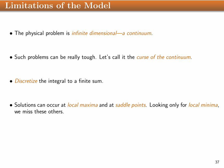
Limitations of the Model
• The physical problem is infinite dimensional—a continuum.
• Such problems can be really tough. Let’s call it the curse of the continuum.
• Discretize the integral to a finite sum.
• Solutions can occur at local maxima and at saddle points. Looking only for local minima,we miss these others.
37
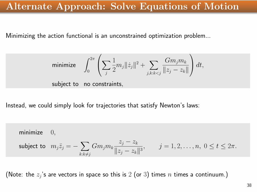
Alternate Approach: Solve Equations of Motion
Minimizing the action functional is an unconstrained optimization problem...
minimize
∫ 2π
0
∑j
1
2mj‖zj‖2 +
∑j,k:k<j
Gmjmk
‖zj − zk‖
dt,subject to no constraints,
Instead, we could simply look for trajectories that satisfy Newton’s laws:
minimize 0,
subject to mjzj = −∑k:k 6=j
Gmjmk
zj − zk‖zj − zk‖3
, j = 1, 2, . . . , n, 0 ≤ t ≤ 2π.
(Note: the zj’s are vectors in space so this is 2 (or 3) times n times a continuum.)
38
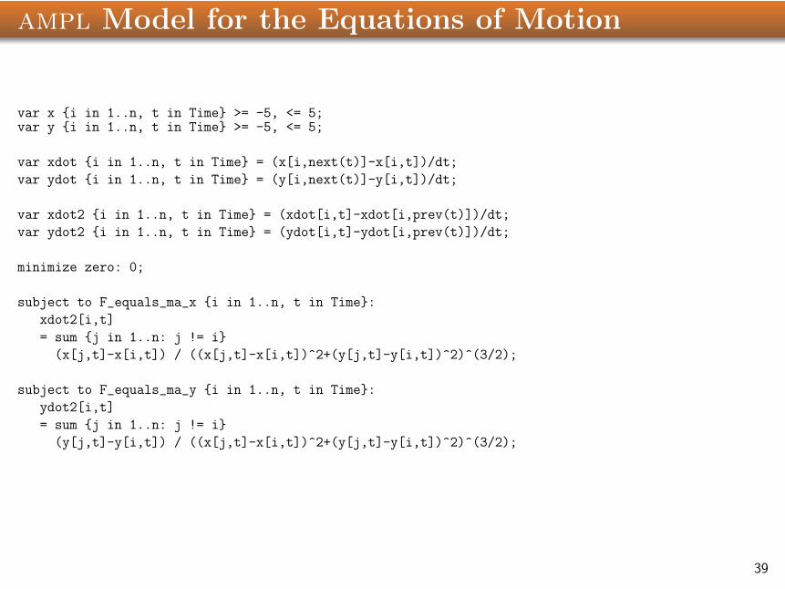
ampl Model for the Equations of Motion
var x {i in 1..n, t in Time} >= -5, <= 5;var y {i in 1..n, t in Time} >= -5, <= 5;
var xdot {i in 1..n, t in Time} = (x[i,next(t)]-x[i,t])/dt;
var ydot {i in 1..n, t in Time} = (y[i,next(t)]-y[i,t])/dt;
var xdot2 {i in 1..n, t in Time} = (xdot[i,t]-xdot[i,prev(t)])/dt;
var ydot2 {i in 1..n, t in Time} = (ydot[i,t]-ydot[i,prev(t)])/dt;
minimize zero: 0;
subject to F_equals_ma_x {i in 1..n, t in Time}:
xdot2[i,t]
= sum {j in 1..n: j != i}
(x[j,t]-x[i,t]) / ((x[j,t]-x[i,t])^2+(y[j,t]-y[i,t])^2)^(3/2);
subject to F_equals_ma_y {i in 1..n, t in Time}:
ydot2[i,t]
= sum {j in 1..n: j != i}
(y[j,t]-y[i,t]) / ((x[j,t]-x[i,t])^2+(y[j,t]-y[i,t])^2)^(3/2);
39
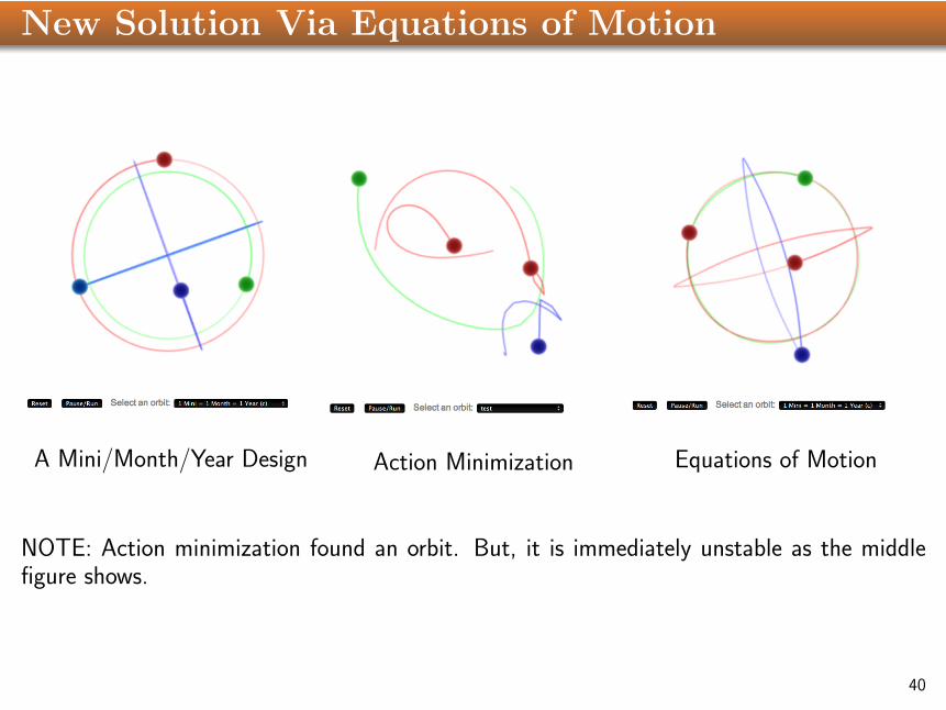
New Solution Via Equations of Motion
A Mini/Month/Year Design Action Minimization Equations of Motion
NOTE: Action minimization found an orbit. But, it is immediately unstable as the middlefigure shows.
40
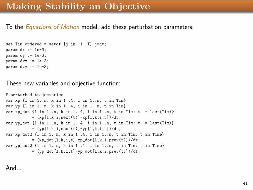
Making Stability an Objective
To the Equations of Motion model, add these perturbation parameters:
set Tim ordered = setof {j in -1..T} j*dt;
param dx := 1e-3;
param dy := 1e-3;
param dvx := 1e-3;
param dvy := 1e-3;
These new variables and objective function:
# perturbed trajectories
var xp {l in 1..n, k in 1..4, i in 1..n, t in Tim};
var yp {l in 1..n, k in 1..4, i in 1..n, t in Tim};
var xp_dot {l in 1..n, k in 1..4, i in 1..n, t in Tim: t != last(Tim)}
= (xp[l,k,i,next(t)]-xp[l,k,i,t])/dt;
var yp_dot {l in 1..n, k in 1..4, i in 1..n, t in Tim: t != last(Tim)}
= (yp[l,k,i,next(t)]-yp[l,k,i,t])/dt;
var xp_dot2 {l in 1..n, k in 1..4, i in 1..n, t in Tim: t in Time}
= (xp_dot[l,k,i,t]-xp_dot[l,k,i,prev(t)])/dt;
var yp_dot2 {l in 1..n, k in 1..4, i in 1..n, t in Tim: t in Time}
= (yp_dot[l,k,i,t]-yp_dot[l,k,i,prev(t)])/dt;
And...
41
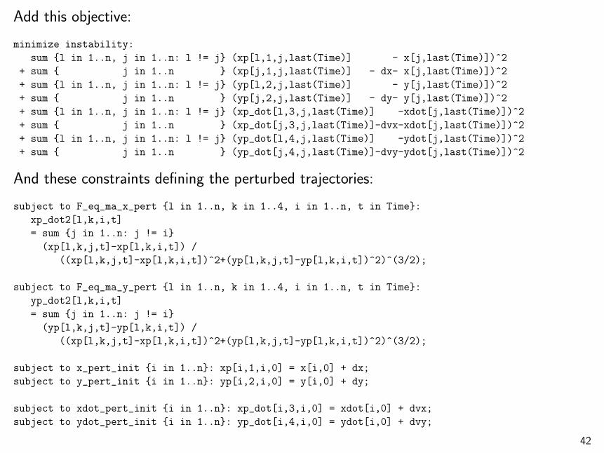
Add this objective:
minimize instability:
sum {l in 1..n, j in 1..n: l != j} (xp[l,1,j,last(Time)] - x[j,last(Time)])^2
+ sum { j in 1..n } (xp[j,1,j,last(Time)] - dx- x[j,last(Time)])^2
+ sum {l in 1..n, j in 1..n: l != j} (yp[l,2,j,last(Time)] - y[j,last(Time)])^2
+ sum { j in 1..n } (yp[j,2,j,last(Time)] - dy- y[j,last(Time)])^2
+ sum {l in 1..n, j in 1..n: l != j} (xp_dot[l,3,j,last(Time)] -xdot[j,last(Time)])^2
+ sum { j in 1..n } (xp_dot[j,3,j,last(Time)]-dvx-xdot[j,last(Time)])^2
+ sum {l in 1..n, j in 1..n: l != j} (yp_dot[l,4,j,last(Time)] -ydot[j,last(Time)])^2
+ sum { j in 1..n } (yp_dot[j,4,j,last(Time)]-dvy-ydot[j,last(Time)])^2
And these constraints defining the perturbed trajectories:
subject to F_eq_ma_x_pert {l in 1..n, k in 1..4, i in 1..n, t in Time}:
xp_dot2[l,k,i,t]
= sum {j in 1..n: j != i}
(xp[l,k,j,t]-xp[l,k,i,t]) /
((xp[l,k,j,t]-xp[l,k,i,t])^2+(yp[l,k,j,t]-yp[l,k,i,t])^2)^(3/2);
subject to F_eq_ma_y_pert {l in 1..n, k in 1..4, i in 1..n, t in Time}:
yp_dot2[l,k,i,t]
= sum {j in 1..n: j != i}
(yp[l,k,j,t]-yp[l,k,i,t]) /
((xp[l,k,j,t]-xp[l,k,i,t])^2+(yp[l,k,j,t]-yp[l,k,i,t])^2)^(3/2);
subject to x_pert_init {i in 1..n}: xp[i,1,i,0] = x[i,0] + dx;
subject to y_pert_init {i in 1..n}: yp[i,2,i,0] = y[i,0] + dy;
subject to xdot_pert_init {i in 1..n}: xp_dot[i,3,i,0] = xdot[i,0] + dvx;
subject to ydot_pert_init {i in 1..n}: yp_dot[i,4,i,0] = ydot[i,0] + dvy;
42
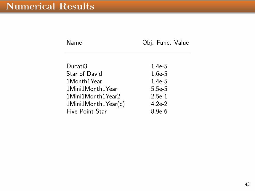
Numerical Results
Name Obj. Func. Value
Ducati3 1.4e-5Star of David 1.6e-51Month1Year 1.4e-51Mini1Month1Year 5.5e-51Mini1Month1Year2 2.5e-11Mini1Month1Year(c) 4.2e-2Five Point Star 8.9e-6
43

Thank You!
44