Expert Systems with Applications 38 (2011) 6627–6636

Contents lists available at ScienceDirect

Expert Systems with Applications

journal homepage: www.elsevier .com/locate /eswa

Initialization of the Benders master problem using valid inequalities appliedto fixed-charge network problems

Georgios K.D. Saharidis ⇑, Maria Boile, Sotiris TheofanisCenter for Advanced Infrastructure and Transportation (CAIT), Department of Civil and Environmental Engineering, Rutgers – The State University of New Jersey,98 Brett Road, Piscataway, NJ 08854-8058, United States

a r t i c l e i n f o

Keywords:Fixed-charge network problemBenders decompositionValid inequalitiesMixed integer programmingRefineryScheduling of crude oil

0957-4174/$ - see front matter � 2009 Elsevier Ltd. Adoi:10.1016/j.eswa.2010.11.075

⇑ Corresponding author.E-mail address: saharidis@gmail.com (G.K.D. Saha

a b s t r a c t

Network problems concern the selection of arcs in a graph in order to satisfy, at minimum cost, some flowrequirements, usually expressed in the form of node–node pair demands. Benders decomposition meth-ods, based on the idea of partitioning of the initial problem to two sub-problems and on the generation ofcuts, have been successfully applied to many of these problems. This paper presents a novel way to reini-tialize the Benders master problem for this group of problems using a series of valid inequalities. A gen-eric presentation of the developed valid inequalities is presented as well as a case study of a refinerysystem is used in order to illustrate the advantage of the proposed procedure. The valid inequalities sig-nificantly restrict the solution space of the Benders master problem from the first iteration of the algo-rithm leading to improved convergence.

� 2009 Elsevier Ltd. All rights reserved.

1. Introduction

Network design problems are central to a large number of con-texts including transportation, telecommunications, power sys-tems and chemical processing. The idea is to establish or use anetwork of links (roads, optical fibers, electric lines, pipelines,etc.) that enables the flow of commodities (people, data, packets,electricity, crude oil, etc.) in order to satisfy some demand charac-teristics. Herein, we are particularly interested in fixed-charge net-work problems, where, in order to use a link, one must pay a fixedcost representing, for example, the cost of using a road, or an elec-tric line, or a pipeline, etc.

A large number of practical applications may be represented byfixed-charge network models. One important area is the servicenetwork design problem which arises, for example, in airline andtrucking companies, pipelines and electric lines. The idea is tomaximize the profit by setting routes and schedules, given someresource constraints. For example, airline companies must deter-mine the covered routes and the frequency of the flights consider-ing aircraft and crew availability (Lederer & Nambimadom, 1998).Similarly, express package delivery companies must establishroutes, assign aircrafts to them and decide about the flow of pack-ages (Armacos, Barnhart, & Ware, 2002). The multi-commodity,multi-model distribution planning problem is another distributionproblem with fixed charge where Benders decomposition has been

ll rights reserved.

ridis).

applied successfully (Cakir, 2009). Various applications can also befound in chemical processing problems. In a refinery system aschedule defines which pipeline will be used for loading andunloading of tanks in order to load the crude oil arriving to therefinery port and unload blends of crude oil toward the crude dis-tillation units. In power systems, the fixed-charge network prob-lem is used to plan the energy transmission from the generationplants to the consumer centers (Binato, Pereira, & Granville,2001; Romero & Monticelli, 1994) and obtain the configurationthat minimizes daily loss costs (Cavelluci & Filho, 1997) and setupcost of the system (Saharidis, Minoux, & Dallery, 2009; Saharidis &Ierapetritou, 2009).

In all these cases, proper use of the system resources can resultin improved operations and reduced costs. The total amount ofthese reductions is obviously related to each specific problem.However, the economical importance of most of the cited problemsand the key role played by the use of the network in the systemsoperation suggest that the savings can be significant (Costa,2005). This economical importance has prompted the developmentof several solution methodologies for network problems. Thesemethodologies range from pure heuristic methods (Golias, 2007)to optimal implicit enumeration (Saharidis, Minoux, & Ierapetritou,2010). Amongst the most successful solution approaches is theBenders decomposition method (Benders, 1962).

The outline of the paper is as follows. In Section 2 we review theclassical Benders algorithm and in Section 3 we give a generaldescription of a network system as well as a case study adoptingthe model presented in Saharidis et al. (2009), for illustrative

Nomenclature

Indexi first level nodes: docksz intermediate level nodes: tanksk final level nodes: CDUj type of commodity (e.g. crude oil)t periodNZ the number of tanksNP the number of docksNCDU the number of crude distillation unitsNJ the number of various types of crude oilNT the number of periods

DataCap the storage capacity of node z (the same for any tank)Ei,t the total quantity of the crude oil available, in dock i, for

period taei,j,t the percentage of the crude oil (Ei,t) of type j, of the

quantity available in dock i, for period tSk,t the total quantity requested from CDUk, for the period task,j,t the percentage of the crude oil (Sk,t) of type j, required

by CDUk, for period tak,j,t equal to 1 if the CDUk requests crude oil of type j, for

period t and equal to 0 if notamink,j,t acceptable minimal percentage, of type j, for the blend

unloading towards CDUk, for period tamaxk,j,t acceptable maximal percentage, of type j, for the blend

unloading towards CDUk, for period twi,j,t equal to 1 if a boat is in dock i and brings crude oil of

type j, for period t; equal to zero otherwiseqk,j,t equal to 1 if the CDUk requests crude oil of type j, for

period t; equal to 0 otherwiseTCt number of different types of crude oil or blends of crude

oil requested by CDUs for period tLj,t equal to 1 if the crude oil of type j is requested by CDUs

for period t; equal to 0 otherwise

Decision variablesXi,z,j,t continuous variable which corresponds to the quantity

of crude oil type j, loaded by dock i, in tank z, for periodt (flow dock ) tank)

Yz,k,j,t continuous variable which corresponds to the quantityof crude oil type j, unloaded by tank z, with CDUk , forperiod t (flow tank ) CDU)

Iz,j,t continuous variable which corresponds to the quantityof crude oil type j, stocked at the end of period t, in tankz. We specify that variables Iz,j,0 are data correspondingto the quantities stored in the tanks at the beginning ofscheduling period

Ci,z,t binary variable (0–1) which is equal to 1 if loading pipe-line is opened between the dock i and tank z, for period tand equal to 0 if not

Dz,k,t binary variable (0–1) which is equal to 1 if unloadingpipeline is opened between the tank z and CDUk, for per-iod t and equal to 0 if not

SCi,z,t binary variable (0–1) which is equal to 1 if setup of load-ing pipeline is established for loading crude oil from thedock i, at the beginning of the period t and equal to zeroif not

SDi,z,t binary variable (0–1) which is equal to 1 if setup ofunloading pipeline is established for unloading crudeoil towards CDUk, at the beginning of the period t andequal to zero if not

Fz,j,t binary variable (0–1) which is equal to 1 if tank z con-tains commodity type j, for the period t and equal tozero if not

cz,k,t Integer variable that takes value in the interval [0,1 0 0]and defines the percentage of the total quantity storedin the tank z unloaded towards the CDUk in period t

6628 G.K.D. Saharidis et al. / Expert Systems with Applications 38 (2011) 6627–6636

purpose. In Section 4 we present a series of general valid inequal-ities which initialize the problem with significant good conver-gence properties as we demonstrate through numericalexamples. Finally in Section 5 we present conclusions and someperspectives for further research.

2. Benders method

2.1. Benders algorithm

The Benders decomposition method is based on the idea ofexploiting the decomposable structure present in the formulationof an initial problem (IP) so that its solution can be converted intothe solution of several smaller sub-problems. Benders method istypically used when the initial model has complicating decisionvariables (Conejo, Castillo, Minguez, & Garcia-Bertrand, 2006).Complicating decision variables could be variables which makethe problem non-convex, such as integer decision variables and/or a group of decision variables which appear in all or in most ofthe constraints. Decomposing the problem using these variablesresults in a series of sub-problems which are easier to solve (e.g.continuous problems). For the fixed-charge network problem thecomplicating decision variables correspond to a series of binaryvariables which appear in many constraints. We briefly state theidea of the Benders algorithm (Benders, 1962) considering, withoutloss of generality, the following linear problem

Initial ProblemðIPÞ :

Mim cT xþ dT y

st:Axþ By 6 b

x 2 Rnþ; y 2 Zq

þ;

where c 2 Rn;d 2 Rq; b 2 Rm, A and B are m � n and m � q, matricesrespectively. The decision variables are partitioned into two sets xand y. For fixed y ðy ¼ �yÞ, IP takes the following form:

Primal Slave ProblemðPSPÞ :

f ðxÞ ¼Mim cT xþ dT �y

st:Ax 6 b� B�y

x 2 Rnþ:

In Benders decomposition we decompose the IP into PSP, which is arestriction of IP and provides an upper bound (UB) in the case ofminimization, and the following relaxation of IP, which is calledthe restricted master problem (RMP) and provides a lower bound(LB):

Restricted Master ProblemðRMPÞ :

Fðy; zÞ ¼Mim z

st:

G.K.D. Saharidis et al. / Expert Systems with Applications 38 (2011) 6627–6636 6629

v iT ðb� ByÞ 6 0

ujT ðb� ByÞ þ dT y� z 6 0

)Benders cuts

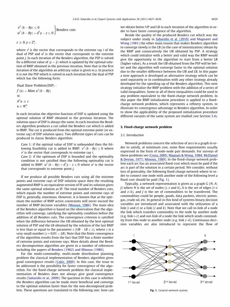
Fig. 1. General network system.

z P 0; y 2 Zqþ;

where vi is the vector that corresponds to the extreme ray i of thedual of PSP and uj is the vector that corresponds to the extremepoint j. In each iteration of the Benders algorithm, the PSP is solvedfor a different value of ðy ¼ �yÞwhich is updated by the optimal solu-tion of RMP obtained in the previous iteration. Note that in the firstiteration of the algorithm an arbitrary value is given to y. In practiceit is not the PSP which is solved in each iteration but the dual of PSPwhich has the following form:

Dual Slave ProblemðDSPÞ :

f 0ðuÞ ¼ Mim uTðb� B�yÞst:

AT u P c

u 2 Rm� :

In each iteration the objective function of DSP is updated using theoptimal solution of RMP obtained in the previous iteration. Thesolution space of DSP is always the same. In each iteration the Bend-ers algorithm produces a cut called the Benders cut which is addedto RMP. The cut is produced from the optimal extreme point (or ex-treme ray) of DSP solution space. Two different types of cuts can beproduced in classic Benders algorithm:

Case 1: if the optimal value of DSP is unbounded then the fol-lowing feasibility cut is added to RMP: v iT ðb� ByÞ 6 0 wherevi is the vector that corresponds to extreme ray i.Case 2: if the optimum of DSP is bounded and the optimalitycondition is not satisfied then the following optimality cut isadded to RMP: ujT ðb� ByÞ þ dT y� z 6 0 where uj is the vectorthat corresponds to extreme point j.

If we produce all possible Benders cuts using all the extremepoints and extreme rays of DSP solution space then the resultingaugmented RMP is an equivalent version of IP and its solution givesthe same optimal solution as IP. The total number of Benders cuts,which equals the number of extreme points and extreme rays ofDSP is, generally, enormous. However, it is known that at the opti-mum the number of RMP active constraints will never exceed thenumber of RMP decision variables (Minoux, 1986). The main ideaof the Benders algorithm is based on the observation that the algo-rithm will converge, satisfying the optimality condition before theaddition of all Benders cuts. The convergence criterion is satisfiedwhen the difference between the UB obtained by the best optimalsolution of PSP and the LB obtained by the solution of the last RMPis less than or equal to the parameter e (UB � LB 6 e), where e is avery small number (e = 0.01 � LB). Note that the finite convergenceof the algorithm results from the fact that DSP has a finite numberof extreme points and extreme rays. More details about the Bend-ers decomposition algorithm are given in a number of referencesincluding the papers of Benders (1962) and Minoux (1986).

For the multi-commodity, multi-mode distribution planningproblem the classical implementation of Benders algorithm givesgood convergence results (Cakir, 2009). In this case, the issue tobe addressed is the possibility for faster convergence of the algo-rithm. For the fixed-charge network problem the classical imple-mentation of Benders does not always give good convergenceresults (Saharidis et al., 2009). The question in this case is whetherthe Benders algorithm can be made more beneficial and convergeto the optimal solution faster than for the non-decomposed prob-lem. These questions are translated to the following one: how can

we obtain better UP and LB in each iteration of the algorithm in or-der to have faster convergence of the algorithm.

Beside the quality of the produced Benders cut which was thesubject under study in Saharidis et al. (2010) and Magnanti andWong (1981) the other main reason that makes Benders algorithmto converge slowly is the LB (in the case of minimization) obtain bythe RMP and consecutively the UB obtained by PSP. A strategywhich could initialize with a better and valid way the RMP wouldgive the opportunity to the algorithm to start from a better LB(higher value). As a result the UB obtained from the PSP will be bet-ter and the algorithm will converge faster to the optimal solutiondue to the smaller difference between the UB and LB. In this papera new approach is developed as alternative strategy which can beused separately or in combination with any other strategy alreadydeveloped for the speeding-up of the Benders algorithm. This newstrategy initialize the RMP problem with the addition of a series ofvalid inequalities. Some or all of these inequalities could be used inany problem equivalent to the fixed-charge network problem. Inthis paper the RMP initialization procedure is applied to a fixed-charge network problem, which represents a refinery system, toillustrate its convergence advantage in Benders algorithm. In orderto show the applicability of the proposed initialization proceduredifferent variants of the same system are studied (see Section 3.4).

3. Fixed-charge network problem

3.1. Introduction

Network problems concern the selection of arcs in a graph in or-der to satisfy, at minimum cost, some flow requirements usuallyexpressed in the form of node-node pair demands. For surveys ofthese problems see (Costa, 2005; Magnati & Wong, 1984; McDaniel& Devine, 1977; Minoux, 1989). In the fixed-charge network prob-lem each arc has an associated fixed-cost which must be paid if thearc is part of the solution in a certain period. We consider, withoutloss of generality, the following fixed-charge network where in or-der to connect one node with another node of the following level afixed cost should be paid (Fig. 1).

Typically, a network representation is given as a graph G (N; A;J) where N is the set of nodes (i, z and k), A is the set of edges (i–zand z–k), and J is the set of commodities to be transferred. Thecommodities could be people, goods, data packets, electric power,gas, crude oil, etc. In general in this kind of systems binary decisionvariables are introduced and associated with the utilization of alink (i and z) or a link (z and k). Note that we call in-link of a nodethe link which transfers commodity to the node by another node(e.g. link i–z) and out-link of a node the link which sends commod-ity from this node to another node (e.g. link z–k). Continuous deci-sion variables are also introduced to represent the flow of

6630 G.K.D. Saharidis et al. / Expert Systems with Applications 38 (2011) 6627–6636

commodity j going from node i to node z and from node z to node k.This general system could represent a number of systemsincluding:

(a) a transportation network which transports products fromone place to another (i could be the place where the trucksload the products and z and k could represent customers,depots, or terminals);

(b) a crossdocking facility or a warehouse which receives prod-ucts from origin nodes and send them to the destinationnodes (z corresponds to one or many crossdocking facilitiesand/or warehouses, i to the origin nodes and k to the desti-nation nodes);

(c) a power supply system which distributes electricity (i couldbe the power electricity production units and z and k twodifferent groups of customers e.g. industry and homes);

(d) a computer or a telecommunication network design system(i and k could be the customers and z the servers or telecom-munication centers);

(e) a refinery system to define the use of pipelines for each per-iod of scheduling (i could be the ports, z the storage tanksand k the distillation units).

The structure of all these systems which correspond to a fixed-charge network problem presents a natural decomposition schemefor the Benders approach. The variables representing the openingof the links (e.g. use of pipelines) or the connection between twonodes (eg select a route to deliver a commodity) could be consid-ered as the RMP decision variables while the ones representingthe actual flow of commodities are kept in the SP. Therefore, ateach iteration the RMP solution gives a tentative network forwhich the SP finds the optimal flow of commodities.

3.2. Typical refinery system

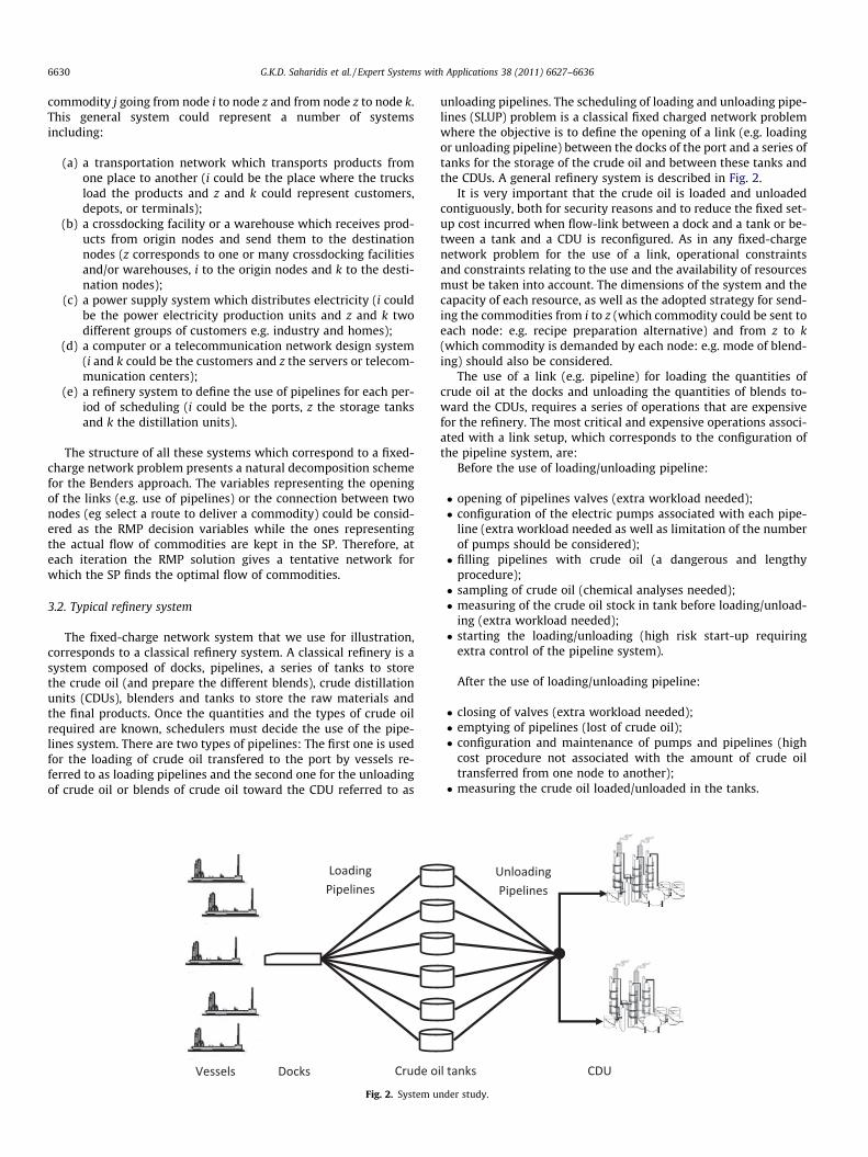
The fixed-charge network system that we use for illustration,corresponds to a classical refinery system. A classical refinery is asystem composed of docks, pipelines, a series of tanks to storethe crude oil (and prepare the different blends), crude distillationunits (CDUs), blenders and tanks to store the raw materials andthe final products. Once the quantities and the types of crude oilrequired are known, schedulers must decide the use of the pipe-lines system. There are two types of pipelines: The first one is usedfor the loading of crude oil transfered to the port by vessels re-ferred to as loading pipelines and the second one for the unloadingof crude oil or blends of crude oil toward the CDU referred to as

Fig. 2. System u

unloading pipelines. The scheduling of loading and unloading pipe-lines (SLUP) problem is a classical fixed charged network problemwhere the objective is to define the opening of a link (e.g. loadingor unloading pipeline) between the docks of the port and a series oftanks for the storage of the crude oil and between these tanks andthe CDUs. A general refinery system is described in Fig. 2.

It is very important that the crude oil is loaded and unloadedcontiguously, both for security reasons and to reduce the fixed set-up cost incurred when flow-link between a dock and a tank or be-tween a tank and a CDU is reconfigured. As in any fixed-chargenetwork problem for the use of a link, operational constraintsand constraints relating to the use and the availability of resourcesmust be taken into account. The dimensions of the system and thecapacity of each resource, as well as the adopted strategy for send-ing the commodities from i to z (which commodity could be sent toeach node: e.g. recipe preparation alternative) and from z to k(which commodity is demanded by each node: e.g. mode of blend-ing) should also be considered.

The use of a link (e.g. pipeline) for loading the quantities ofcrude oil at the docks and unloading the quantities of blends to-ward the CDUs, requires a series of operations that are expensivefor the refinery. The most critical and expensive operations associ-ated with a link setup, which corresponds to the configuration ofthe pipeline system, are:

Before the use of loading/unloading pipeline:

� opening of pipelines valves (extra workload needed);� configuration of the electric pumps associated with each pipe-

line (extra workload needed as well as limitation of the numberof pumps should be considered);� filling pipelines with crude oil (a dangerous and lengthy

procedure);� sampling of crude oil (chemical analyses needed);� measuring of the crude oil stock in tank before loading/unload-

ing (extra workload needed);� starting the loading/unloading (high risk start-up requiring

extra control of the pipeline system).

After the use of loading/unloading pipeline:

� closing of valves (extra workload needed);� emptying of pipelines (lost of crude oil);� configuration and maintenance of pumps and pipelines (high

cost procedure not associated with the amount of crude oiltransferred from one node to another);� measuring the crude oil loaded/unloaded in the tanks.

nder study.

G.K.D. Saharidis et al. / Expert Systems with Applications 38 (2011) 6627–6636 6631

Costs associated with these operations require that the use ofthe pipelines for loading and unloading should be completed withthe minimum number of link setups. As we stated before, theminimization of the number of setups is required also for securityreasons, as the above operations are complicated and with eachstart of a new loading and unloading, the system is strained. Insummary, the problem under consideration is to schedule thetransfer of crude oil from the docks to the tanks and from thetanks to the CDUs minimizing the setup cost of the existing pipe-line network.

3.3. General model for scheduling of loading and unloading pipelines

In a typical refinery there are 1–10 tanks for the storage of thecrude oil. The storage capacity of each tank can range from80,000 m3 to 150,000 m3. Crude oil flows from the docks to thetanks, and its flow depends on the unloading capacity of the ves-sels, ranging from 1000 m3/h to 5000 m3/h. Duration of a vessel’sunloading is typically defined a priori by contract. After the loadingof tanks from the vessels, crude oil flows from the tanks towardsthe CDU. This flow corresponds to the distillation capacity of eachunit. Each CDU has a distillation capacity that can range from200 m3/h to 2000 m3/h. A typical refinery is composed of 1–4 CDUsand 1 or 2 docks, which can accommodate 4–5 vessels per month.The data and the parameters of the system are: dimensions of therefinery, arrival dates of vessels based on medium-term planning,demand of crude oil by the CDU, initial conditions (quantity andcomposition in each tank) and the system’s capabilities (opera-tional time, tank capacity and flow limit). Moreover, the numberof tanks available for storage and their storage capacity are known.The production rates are determined prior to the selection of therecipe preparation alternative and the blending mode, which areknown as well.

The modeling of this problem involves both continuous andbinary decision variables. The continuous variables correspondto flows from docks to tanks, flows from tanks to CDUs, andquantities stored in the tanks. Binary variables are used to specifyconnections between docks and tanks, connections betweentanks and CDUs, and also the availability and setup for the useof loading and unloading pipelines. The constraints necessary todescribe the system include: (a) satisfying operations rules; (b)satisfying material balances; (c) meeting storage capacity con-straints; (d) satisfying blend properties; (e) establishing aconnection between docks and tanks; (f) establishing connectionsbetween tanks and CDUs; and (g) setup of tanks for loading orunloading.

In this section, we describe our model for the scheduling ofloading and unloading pipelines for all modes of blending. In thefollowing nomenclature, we present the parameters, the data andthe decision variables which are used in each type of blendingmode. After the presentation of the general features of the modelwe provide the specific additional data, decision variables and con-straints associated with its main variants, depending on the spe-cific context of application in each system’s setup. The objectivein all cases is the minimization of the fixed-charge cost associatedwith the use of a link, which corresponds to the use of loading/unloading pipelines.

In general, we have four groups of constraints which guaranteecertain operational conditions. We have constraints which guaran-tee that the quantities loaded in tanks are equal to the quantitiesavailable to docks in each period and constraints guaranteeing thatthe quantities unloaded towards CDUs are equal to the quantitiesrequired by them. We also have constraints expressing the mate-rial balance, and others which guarantee that quantity stored ina tank is not greater than its storage capacity.

XNZ

z¼1

Xi;z;j;t ¼ Ei;taei;j;t 8i; j; t ð1Þ

XNZ

z¼1

XNJ

j¼1

Yz;k;j;t ¼ Sk;t 8k; t ð2Þ

amink;j;tak;j;tSk;t 6XNZ

z¼1

Yz;k;j;t 6 amaxk;j;tak;j;tSk;t 8k; j; t ð3Þ

Iz;j;t ¼ Iz;j;t�1 þXNP

i¼1

Xi;z;j;t �XNCDU

k¼1

Yz;k;j;t 8z; j; t ð4Þ

0 6XNJ

j¼1

Iz;j;t 6 Cap 8z; t ð5Þ

Ci;z;t 6XNJ

j¼1

Xi;z;j;t 6 MCi;z;t; 8i; z; t ð6Þ

Dz;k;t 6XNJ

j¼1

Yz;k;j;t 6 MDz;k;t ; 8z; k; t ð7Þ

Ci;z;t þ Dz;k;t 6 1 8i; z; k; t ð8Þ

Ci;z;t�1 þ SCi;z;t P Ci;z;t 8i; z; t ð9Þ

Dz;k;t�1 þ SDz;k;t P Dz;j;t 8z; k; t ð10Þ

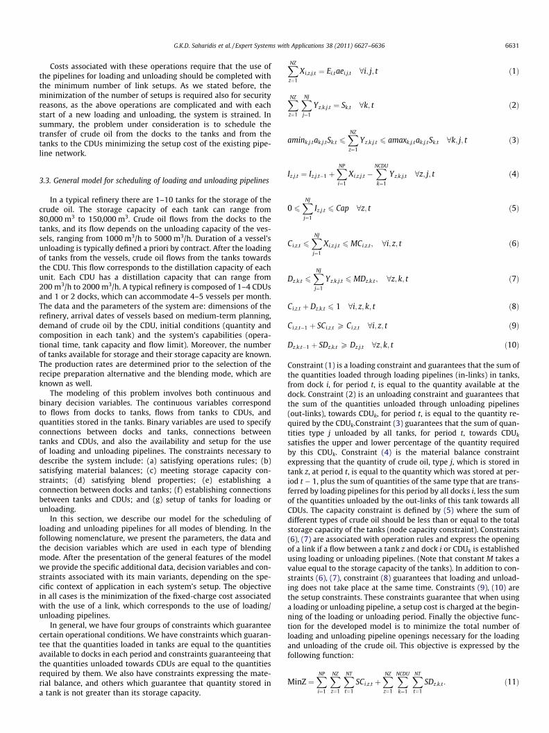
Constraint (1) is a loading constraint and guarantees that the sum ofthe quantities loaded through loading pipelines (in-links) in tanks,from dock i, for period t, is equal to the quantity available at thedock. Constraint (2) is an unloading constraint and guarantees thatthe sum of the quantities unloaded through unloading pipelines(out-links), towards CDUk, for period t, is equal to the quantity re-quired by the CDUk.Constraint (3) guarantees that the sum of quan-tities type j unloaded by all tanks, for period t, towards CDUk

satisfies the upper and lower percentage of the quantity requiredby this CDUk. Constraint (4) is the material balance constraintexpressing that the quantity of crude oil, type j, which is stored intank z, at period t, is equal to the quantity which was stored at per-iod t � 1, plus the sum of quantities of the same type that are trans-ferred by loading pipelines for this period by all docks i, less the sumof the quantities unloaded by the out-links of this tank towards allCDUs. The capacity constraint is defined by (5) where the sum ofdifferent types of crude oil should be less than or equal to the totalstorage capacity of the tanks (node capacity constraint). Constraints(6), (7) are associated with operation rules and express the openingof a link if a flow between a tank z and dock i or CDUk is establishedusing loading or unloading pipelines. (Note that constant M takes avalue equal to the storage capacity of the tanks). In addition to con-straints (6), (7), constraint (8) guarantees that loading and unload-ing does not take place at the same time. Constraints (9), (10) arethe setup constraints. These constraints guarantee that when usinga loading or unloading pipeline, a setup cost is charged at the begin-ning of the loading or unloading period. Finally the objective func-tion for the developed model is to minimize the total number ofloading and unloading pipeline openings necessary for the loadingand unloading of the crude oil. This objective is expressed by thefollowing function:

MinZ ¼XNP

i¼1

XNZ

z¼1

XNT

t¼1

SCi;z;t þXNZ

z¼1

XNCDU

k¼1

XNT

t¼1

SDz;k;t : ð11Þ

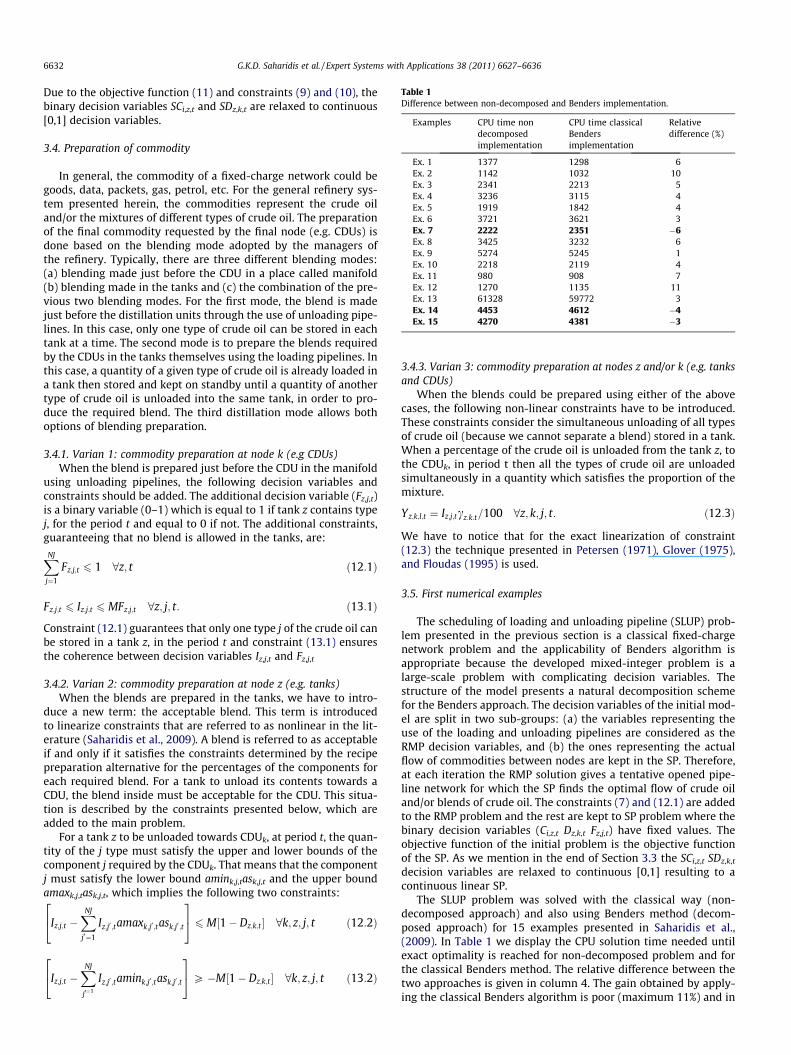
Table 1Difference between non-decomposed and Benders implementation.

Examples CPU time nondecomposedimplementation

CPU time classicalBendersimplementation

Relativedifference (%)

Ex. 1 1377 1298 6Ex. 2 1142 1032 10Ex. 3 2341 2213 5Ex. 4 3236 3115 4Ex. 5 1919 1842 4Ex. 6 3721 3621 3Ex. 7 2222 2351 �6Ex. 8 3425 3232 6Ex. 9 5274 5245 1Ex. 10 2218 2119 4Ex. 11 980 908 7Ex. 12 1270 1135 11Ex. 13 61328 59772 3Ex. 14 4453 4612 �4Ex. 15 4270 4381 �3

6632 G.K.D. Saharidis et al. / Expert Systems with Applications 38 (2011) 6627–6636

Due to the objective function (11) and constraints (9) and (10), thebinary decision variables SCi,z,t and SDz,k,t are relaxed to continuous[0,1] decision variables.

3.4. Preparation of commodity

In general, the commodity of a fixed-charge network could begoods, data, packets, gas, petrol, etc. For the general refinery sys-tem presented herein, the commodities represent the crude oiland/or the mixtures of different types of crude oil. The preparationof the final commodity requested by the final node (e.g. CDUs) isdone based on the blending mode adopted by the managers ofthe refinery. Typically, there are three different blending modes:(a) blending made just before the CDU in a place called manifold(b) blending made in the tanks and (c) the combination of the pre-vious two blending modes. For the first mode, the blend is madejust before the distillation units through the use of unloading pipe-lines. In this case, only one type of crude oil can be stored in eachtank at a time. The second mode is to prepare the blends requiredby the CDUs in the tanks themselves using the loading pipelines. Inthis case, a quantity of a given type of crude oil is already loaded ina tank then stored and kept on standby until a quantity of anothertype of crude oil is unloaded into the same tank, in order to pro-duce the required blend. The third distillation mode allows bothoptions of blending preparation.

3.4.1. Varian 1: commodity preparation at node k (e.g CDUs)When the blend is prepared just before the CDU in the manifold

using unloading pipelines, the following decision variables andconstraints should be added. The additional decision variable (Fz,j,t)is a binary variable (0–1) which is equal to 1 if tank z contains typej, for the period t and equal to 0 if not. The additional constraints,guaranteeing that no blend is allowed in the tanks, are:

XNJ

j¼1

Fz;j;t 6 1 8z; t ð12:1Þ

Fz;j;t 6 Iz;j;t 6 MFz;j;t 8z; j; t: ð13:1Þ

Constraint (12.1) guarantees that only one type j of the crude oil canbe stored in a tank z, in the period t and constraint (13.1) ensuresthe coherence between decision variables Iz,j,t and Fz,j,t

3.4.2. Varian 2: commodity preparation at node z (e.g. tanks)When the blends are prepared in the tanks, we have to intro-

duce a new term: the acceptable blend. This term is introducedto linearize constraints that are referred to as nonlinear in the lit-erature (Saharidis et al., 2009). A blend is referred to as acceptableif and only if it satisfies the constraints determined by the recipepreparation alternative for the percentages of the components foreach required blend. For a tank to unload its contents towards aCDU, the blend inside must be acceptable for the CDU. This situa-tion is described by the constraints presented below, which areadded to the main problem.

For a tank z to be unloaded towards CDUk, at period t, the quan-tity of the j type must satisfy the upper and lower bounds of thecomponent j required by the CDUk. That means that the componentj must satisfy the lower bound amink,j,task,j,t and the upper boundamaxk,j,task,j,t, which implies the following two constraints:

Iz;j;t �XNJ

j0¼1

Iz;j0 ;tamaxk;j0 ;task;j0 ;t

24

35 6 M½1� Dz;k;t � 8k; z; j; t ð12:2Þ

Iz;j;t �XNJ

j0¼1

Iz;j0 ;tamink;j0 ;task;j0 ;t

24

35P �M½1� Dz;k;t � 8k; z; j; t ð13:2Þ

3.4.3. Varian 3: commodity preparation at nodes z and/or k (e.g. tanksand CDUs)

When the blends could be prepared using either of the abovecases, the following non-linear constraints have to be introduced.These constraints consider the simultaneous unloading of all typesof crude oil (because we cannot separate a blend) stored in a tank.When a percentage of the crude oil is unloaded from the tank z, tothe CDUk, in period t then all the types of crude oil are unloadedsimultaneously in a quantity which satisfies the proportion of themixture.

Yz;k;l;t ¼ Iz;j;tcz:k:t=100 8z; k; j; t: ð12:3Þ

We have to notice that for the exact linearization of constraint(12.3) the technique presented in Petersen (1971), Glover (1975),and Floudas (1995) is used.

3.5. First numerical examples

The scheduling of loading and unloading pipeline (SLUP) prob-lem presented in the previous section is a classical fixed-chargenetwork problem and the applicability of Benders algorithm isappropriate because the developed mixed-integer problem is alarge-scale problem with complicating decision variables. Thestructure of the model presents a natural decomposition schemefor the Benders approach. The decision variables of the initial mod-el are split in two sub-groups: (a) the variables representing theuse of the loading and unloading pipelines are considered as theRMP decision variables, and (b) the ones representing the actualflow of commodities between nodes are kept in the SP. Therefore,at each iteration the RMP solution gives a tentative opened pipe-line network for which the SP finds the optimal flow of crude oiland/or blends of crude oil. The constraints (7) and (12.1) are addedto the RMP problem and the rest are kept to SP problem where thebinary decision variables (Ci,z,t Dz,k,t Fz,j,t) have fixed values. Theobjective function of the initial problem is the objective functionof the SP. As we mention in the end of Section 3.3 the SCi,z,t SDz,k,t

decision variables are relaxed to continuous [0,1] resulting to acontinuous linear SP.

The SLUP problem was solved with the classical way (non-decomposed approach) and also using Benders method (decom-posed approach) for 15 examples presented in Saharidis et al.,(2009). In Table 1 we display the CPU solution time needed untilexact optimality is reached for non-decomposed problem and forthe classical Benders method. The relative difference between thetwo approaches is given in column 4. The gain obtained by apply-ing the classical Benders algorithm is poor (maximum 11%) and in

G.K.D. Saharidis et al. / Expert Systems with Applications 38 (2011) 6627–6636 6633

some cases negative (ex. 7) making the application of Bendersalgorithm no always beneficial.

We observed that the main reason that the classical implemen-tation of Benders method did not give the best convergence resultswas the initial large gap between the lower bound obtained fromthe RMP and the upper bound obtained from the SP. For almostall numerical examples the difference between the LB and UBwas more than 90% during the first iterations of the algorithm.For the first example the RMP problem started with a lower boundequal to 1 while the best solution obtained by SP was 21 (a gapequal to 95%) with optimal solution equal to 14 setups of the pipe-line system.

Based on this observation, a strategy which initializes the RMPmore efficiently, restricting as much as possible its initial solutionspace can solve this problem by significantly decreasing the gapbetween the lower and the upper bound. For the initialization ofthe RMP, a series of valid inequalities are developed and presentedin the following section with comparative numerical results. Thenumerical results show that the better initialization of RMP givesrise to a better lower bound (with higher values) resulting betterupper bounds and better convergence properties.

4. Initialization of the Benders master problem

4.1. Introduction

In this section we present a series of valid inequalities whichcould be used in many equivalent fixed-charge network problemsfor the initialization of the RMP problem in order to improve theconvergence of the algorithm. The best way to initialize RMP isto develop a series of valid inequalities which use the decision vari-ables representing the links. These decision variables are binaryvariables and belong to the RMP problem. Adding these validinequalities, an overall positive effect is obtained due to the restric-tion of RMP solution space giving rise to a decrease of the totalnumber of algorithm’s iterations. In the following section we pres-ent a number of general valid inequalities followed by specificexplanations for their application on the SLUP problem. In general,we developed two groups of valid inequalities: the first one con-tains 8 general valid inequalities applicable in any fixed-chargenetwork problem and 7 valid inequalities which are valid if somerules are applicable. In the following, the in-links of intermediatenodes are the out-links of the previous level nodes (e.g. originnode) and the out-links of the intermediate nodes are the in-linksof the next level nodes (e.g. destination nodes).

4.2. First group of valid inequalities

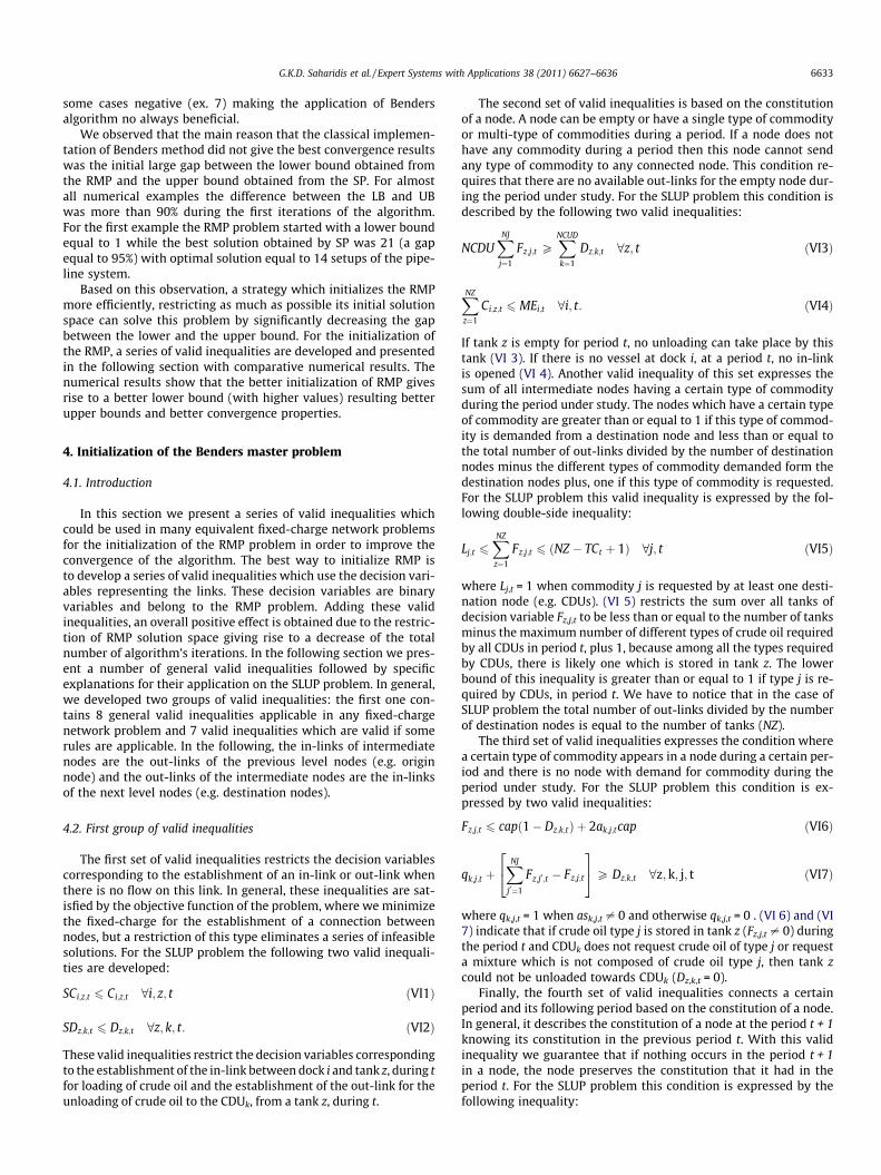
The first set of valid inequalities restricts the decision variablescorresponding to the establishment of an in-link or out-link whenthere is no flow on this link. In general, these inequalities are sat-isfied by the objective function of the problem, where we minimizethe fixed-charge for the establishment of a connection betweennodes, but a restriction of this type eliminates a series of infeasiblesolutions. For the SLUP problem the following two valid inequali-ties are developed:

SCi;z;t 6 Ci;z;t 8i; z; t ðVI1Þ

SDz;k;t 6 Dz;k;t 8z; k; t: ðVI2Þ

These valid inequalities restrict the decision variables correspondingto the establishment of the in-link between dock i and tank z, during tfor loading of crude oil and the establishment of the out-link for theunloading of crude oil to the CDUk, from a tank z, during t.

The second set of valid inequalities is based on the constitutionof a node. A node can be empty or have a single type of commodityor multi-type of commodities during a period. If a node does nothave any commodity during a period then this node cannot sendany type of commodity to any connected node. This condition re-quires that there are no available out-links for the empty node dur-ing the period under study. For the SLUP problem this condition isdescribed by the following two valid inequalities:

NCDUXNJ

j¼1

Fz;j;t PXNCUD

k¼1

Dz;k;t 8z; t ðVI3Þ

XNZ

z¼1

Ci;z;t 6 MEi;t 8i; t: ðVI4Þ

If tank z is empty for period t, no unloading can take place by thistank (VI 3). If there is no vessel at dock i, at a period t, no in-linkis opened (VI 4). Another valid inequality of this set expresses thesum of all intermediate nodes having a certain type of commodityduring the period under study. The nodes which have a certain typeof commodity are greater than or equal to 1 if this type of commod-ity is demanded from a destination node and less than or equal tothe total number of out-links divided by the number of destinationnodes minus the different types of commodity demanded form thedestination nodes plus, one if this type of commodity is requested.For the SLUP problem this valid inequality is expressed by the fol-lowing double-side inequality:

Lj;t 6XNZ

z¼1

Fz;j;t 6 ðNZ � TCt þ 1Þ 8j; t ðVI5Þ

where Lj,t = 1 when commodity j is requested by at least one desti-nation node (e.g. CDUs). (VI 5) restricts the sum over all tanks ofdecision variable Fz,j,t to be less than or equal to the number of tanksminus the maximum number of different types of crude oil requiredby all CDUs in period t, plus 1, because among all the types requiredby CDUs, there is likely one which is stored in tank z. The lowerbound of this inequality is greater than or equal to 1 if type j is re-quired by CDUs, in period t. We have to notice that in the case ofSLUP problem the total number of out-links divided by the numberof destination nodes is equal to the number of tanks (NZ).

The third set of valid inequalities expresses the condition wherea certain type of commodity appears in a node during a certain per-iod and there is no node with demand for commodity during theperiod under study. For the SLUP problem this condition is ex-pressed by two valid inequalities:

Fz;j;t 6 capð1� Dz;k;tÞ þ 2ak;j;tcap ðVI6Þ

qk;j;t þXNJ

j0¼1

Fz;j0 ;t � Fz;j;t

24

35P Dz;k;t 8z;k; j; t ðVI7Þ

where qk,j,t = 1 when ask,j,t – 0 and otherwise qk,j,t = 0 . (VI 6) and (VI7) indicate that if crude oil type j is stored in tank z (Fz,j,t – 0) duringthe period t and CDUk does not request crude oil of type j or requesta mixture which is not composed of crude oil type j, then tank zcould not be unloaded towards CDUk (Dz,k,t = 0).

Finally, the fourth set of valid inequalities connects a certainperiod and its following period based on the constitution of a node.In general, it describes the constitution of a node at the period t + 1knowing its constitution in the previous period t. With this validinequality we guarantee that if nothing occurs in the period t + 1in a node, the node preserves the constitution that it had in theperiod t. For the SLUP problem this condition is expressed by thefollowing inequality:

6634 G.K.D. Saharidis et al. / Expert Systems with Applications 38 (2011) 6627–6636

XNCDU

k¼1ð�Dz;k;tqk;j;tÞ þ Fz;j;t 6 Fz;j;tþ1 6 Fz;j;t þ

XNP

i¼1

ðCi;z;tþ1wi;j;tþ1Þ

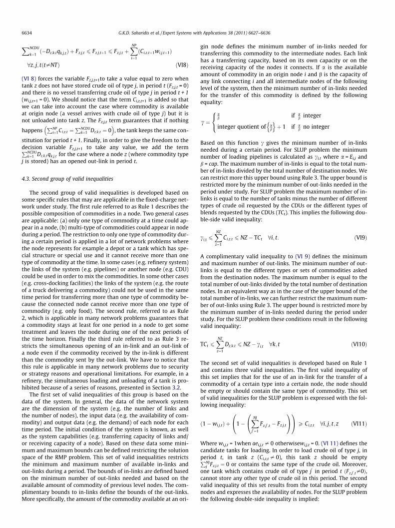
8z; j; tðt–NTÞ ðVI8Þ

(VI 8) forces the variable Fz,j,t+1to take a value equal to zero whentank z does not have stored crude oil of type j, in period t (Fz,j,t = 0)and there is no vessel transferring crude oil of type j in period t + 1(wi,j,t+1 = 0). We should notice that the term Ci,z,t+1 is added so thatwe can take into account the case where commodity is availableat origin node (a vessel arrives with crude oil of type j) but it isnot unloaded into tank z. The Fz,j,t term guarantees that if nothing

happensPNP

i¼1Ci;z;t ¼PNCDU

k¼1 Dz;k;t ¼ 0� �

, the tank keeps the same con-

stitution for period t + 1. Finally, in order to give the freedom to thedecision variable Fz,j,t+1 to take any value, we add the termPNCDU

k¼1 Dz;k;tqk;j;t for the case where a node z (where commodity typej is stored) has an opened out-link in period t.

4.3. Second group of valid inequalities

The second group of valid inequalities is developed based onsome specific rules that may are applicable in the fixed-charge net-work under study. The first rule referred to as Rule 1 describes thepossible composition of commodities in a node. Two general casesare applicable: (a) only one type of commodity at a time could ap-pear in a node, (b) multi-type of commodities could appear in nodeduring a period. The restriction to only one type of commodity dur-ing a certain period is applied in a lot of network problems wherethe node represents for example a depot or a tank which has spe-cial structure or special use and it cannot receive more than onetype of commodity at the time. In some cases (e.g. refinery system)the links of the system (e.g. pipelines) or another node (e.g. CDU)could be used in order to mix the commodities. In some other cases(e.g. cross-docking facilities) the links of the system (e.g. the routeof a truck delivering a commodity) could not be used in the sametime period for transferring more than one type of commodity be-cause the connected node cannot receive more than one type ofcommodity (e.g. only food). The second rule, referred to as Rule2, which is applicable in many network problems guarantees thata commodity stays at least for one period in a node to get sometreatment and leaves the node during one of the next periods ofthe time horizon. Finally the third rule referred to as Rule 3 re-stricts the simultaneous opening of an in-link and an out-link ofa node even if the commodity received by the in-link is differentthan the commodity sent by the out-link. We have to notice thatthis rule is applicable in many network problems due to securityor strategy reasons and operational limitations. For example, in arefinery, the simultaneous loading and unloading of a tank is pro-hibited because of a series of reasons, presented in Section 3.2.

The first set of valid inequalities of this group is based on thedata of the system. In general, the data of the network systemare the dimension of the system (e.g. the number of links andthe number of nodes), the input data (e.g. the availability of com-modity) and output data (e.g. the demand) of each node for eachtime period. The initial condition of the system is known, as wellas the system capabilities (e.g. transferring capacity of links and/or receiving capacity of a node). Based on these data some mini-mum and maximum bounds can be defined restricting the solutionspace of the RMP problem. This set of valid inequalities restrictsthe minimum and maximum number of available in-links andout-links during a period. The bounds of in-links are defined basedon the minimum number of out-links needed and based on theavailable amount of commodity of previous level nodes. The com-plimentary bounds to in-links define the bounds of the out-links.More specifically, the amount of the commodity available at an ori-

gin node defines the minimum number of in-links needed fortransferring this commodity to the intermediate nodes. Each linkhas a transferring capacity, based on its own capacity or on thereceiving capacity of the nodes it connects. If a is the availableamount of commodity in an origin node i and b is the capacity ofany link connecting i and all intermediate nodes of the followinglevel of the system, then the minimum number of in-links neededfor the transfer of this commodity is defined by the followingequality:

c ¼ab if a

b integer

integer quotient of ab

n oþ 1 if a

b no integer

8<:

Based on this function c gives the minimum number of in-linksneeded during a certain period. For SLUP problem the minimumnumber of loading pipelines is calculated as ci,t where a = Ei,j andb = cap. The maximum number of in-links is equal to the total num-ber of in-links divided by the total number of destination nodes. Wecan restrict more this upper bound using Rule 3. The upper bound isrestricted more by the minimum number of out-links needed in theperiod under study. For SLUP problem the maximum number of in-links is equal to the number of tanks minus the number of differenttypes of crude oil requested by the CDUs or the different types ofblends requested by the CDUs (TCt). This implies the following dou-ble-side valid inequality:

ci;t 6XNZ

z¼1

Ci;z;t 6 NZ � TCt 8i; t: ðVI9Þ

A complimentary valid inequality to (VI 9) defines the minimumand maximum number of out-links. The minimum number of out-links is equal to the different types or sets of commodities askedfrom the destination nodes. The maximum number is equal to thetotal number of out-links divided by the total number of destinationnodes. In an equivalent way as in the case of the upper bound of thetotal number of in-links, we can further restrict the maximum num-ber of out-links using Rule 3. The upper bound is restricted more bythe minimum number of in-links needed during the period understudy. For the SLUP problem these conditions result in the followingvalid inequality:

TCt 6XNZ

z¼1

Dz;k;t 6 NZ � ci;t 8k; t ðVI10Þ

The second set of valid inequalities is developed based on Rule 1and contains three valid inequalities. The first valid inequality ofthis set implies that for the use of an in-link for the transfer of acommodity of a certain type into a certain node, the node shouldbe empty or should contain the same type of commodity. This setof valid inequalities for the SLUP problem is expressed with the fol-lowing inequality:

ð1�wi;j;tÞ þ 1�XNJ

j0¼1

Fz;j0 ;t � Fz;j;t

0@

1A

0@

1A P Ci;z;t 8i; j; t; z ðVI11Þ

Where wi,j,t = 1when aei,j,t – 0 otherwisewi,j,t = 0. (VI 11) defines thecandidate tanks for loading. In order to load crude oil of type j, inperiod t, in tank z (Ci,z,t – 0), this tank z should be emptyPNJ

j Fz;j;t ¼ 0 or contains the same type of the crude oil. Moreover,one tank which contains crude oil of type j

0in period t ðFz;j0 ;t–0Þ,

cannot store any other type of crude oil in this period. The secondvalid inequality of this set results from the total number of emptynodes and expresses the availability of nodes. For the SLUP problemthe following double-side inequality is implied:

Table 3Impact of valid inequalities on CPU solution time.

Examples Benders withoutvalid inequalities

Benders with validinequalities

Relativedifference

CPUtime

Number ofiterations

CPUtime

Number ofiterations

CPUtime (%)

Number ofiterations (%)

Ex. 1 1298 615 312 322 76 48Ex. 2 1032 412 412 215 60 48Ex. 3 2213 817 1641 398 26 51Ex. 4 3115 1021 1329 452 57 56Ex. 5 1842 801 852 498 54 38Ex. 6 3621 1112 1852 539 49 52Ex. 7 2178 759 1289 312 41 59Ex. 8 3232 1365 1694 714 48 48Ex. 9 5245 1314 2448 602 53 54Ex. 10 2119 812 935 315 56 61Ex. 11 908 358 526 159 42 56Ex. 12 1135 397 423 137 63 65Ex. 13 59772 2297 29563 908 51 60Ex. 14 4235 1120 1985 568 53 49Ex. 15 3998 1063 1689 452 58 57

G.K.D. Saharidis et al. / Expert Systems with Applications 38 (2011) 6627–6636 6635

TCt 6XNZ

z¼1

XNJ

j¼1

Fz;j;t 6 NZ �XNP

i¼1

ci;t 8t ðVI12Þ

If in period t, the total available quantity of a commodity at an ori-gin node is equal to

PNPi¼1Ei;t then the sum across all tanks and over

all types of crude oil of decision variable Fz,j,t should be greater thanor equal to TCt and less than or equal to the total number of in-linksdivided by the number of docks (which corresponds to the totalnumber of tanks) minus the minimum number of in-links necessaryfor the storage of

PNPi¼1Ei;t . Finally, the last valid inequality of this set

connects period t and t + 1 with a different way than the (VI 8) does.If the commodity available in an origin node and the commoditystored in an intermediate node are not of the same type, the open-ing of an in-link is denied. For SLUP problem this condition is ex-pressed by the following valid inequality:

1�XNJ

j0¼1

Fz;j0 ;t þ Fz;j;t þXNCDU

k¼1

Dz;k;t PXNP

i¼1

ðCi;z;tþ1wi;j;tþ1Þ 8z; j; t ðVI13Þ

If in period t crude oil of type j is stored in tank z and in period t + 1,a vessel arrives with crude oil of type j0

PNPi¼1wi;j0 ;tþ1–0

� �the deci-

sion variable Ci,j,t+1 takes a value equal to 0. The same valid inequal-ity also guarantees that if in period t, tank z is emptyPNJ

j¼1Fz;j;t ¼ 0� �

, and in period t + 1 a vessel arrives to the dock itransferring crude oil of any type, then the tank z can be loaded withthis type of crude oil.

The third set of valid inequalities is generated based on Rule 2.This set of inequalities contains an extension of (VI 3) presented inthe previous section. The (VI 3) is extended to the following periodbecause based on Rule 2 we need one period to load some com-modity to the node in order to be ready after that period to usean out-link. For the SLUP problem this condition implies the fol-lowing inequality:

2� NCDUXNJ

j¼1

Fz;j;t PXNCUD

k¼1

Dz;k;t þXNCUD

k¼1

Dz;k;tþ1 8z; t ðVI14Þ

Finally the fourth set of valid inequalities is introduced based onRule 3 where the simultaneous opening of an in-link and out-linkof a node is prohibited. This set of inequalities guarantees that ifan intermediate node is empty and a destination node requests cer-tain type of commodity, there is not out-link of the intermediatenode which could be opened during the period under study. Forthe SLUP problem this condition is expressed by the followinginequality:

Dz;k;tþ1 6 1� TCk;tþ1ask;j;tþ1 þXNJ

j0¼1

Fz;j0 ;t þ Fz;j;t 8z; k; j; t ðVI15Þ

Table 2Initial solution of RMP – effect of valid inequalities.

Examples Initial RMPsolution

Initial RMPsolution with VI

OptimalSolution

Improvementof LB (%)

Ex. 1 1 6 14 36Ex. 2 0 6 12 50Ex. 3 1 10 14 64Ex. 4 1 16 18 83Ex. 5 2 10 14 57Ex. 6 1 17 20 80Ex. 7 1 11 16 63Ex. 8 1 12 18 61Ex. 9 2 22 24 83Ex. 10 1 11 16 63Ex. 11 1 10 15 60Ex. 12 1 10 14 64Ex. 13 1 11 17 59Ex. 14 1 12 16 69Ex. 15 1 11 16 63

Where if in period t, tank z is emptyPNJ

j Fz;j;t ¼ 0� �

and in periodt + 1 a CDUk requests crude oil of type j

0(qz,j,t – 0) then Dz,k,t+1 = 0.

4.4. Numerical examples

For the same 15 examples presented in the previous section, weapplied the 15 groups of valid inequalities. Column 2 and 3 of Ta-ble 2 present the initial solution of RMP problem obtained by theclassical Benders algorithm and by the addition of the validinequalities respectively. Column 4 gives the optimal solution ofeach example and column 5 the improvement of the lower boundinitializing the RMP. The numerical examples show that the initiallower bound of RMP obtained after the initialization of RMP in-creased significantly from 36% up to 83% compared to the lowerbound obtained by the classical implementation of Bendersalgorithm.

The significant reduction of the solution space of the initial RMPin turn led to a significant reduction in the CPU solution time asshows Table 3. Comparative computational results between thetwo approaches are presented in the last two columns of Table 3where the advantage of applying this strategy of initialization ofRMP is clear. The number of iterations of Benders algorithm de-creased significantly (48–65%) resulting in an important reductionof CPU solution time, which varies between 26% and 76%.

5. Conclusions

A new strategy for Benders method has been discussed and ap-plied in a classical fixed-charge network problem corresponding tothe problem of scheduling of loading and unloading pipeline forthe transfer of crude oil. The presented examples illustrate theapplicability and efficiency of the new strategy which initializethe master problem of Benders algorithm using a series of validinequalities which are generally applicable to many fixed-chargenetwork systems. All the presented examples illustrate that betterinitialization of the RMP problem results in a significant increase ofthe lower bound of Benders algorithm (in the case of minimiza-tion) and in a significant decrease of the number of iterations aswell as the CPU solution time. Future research should investigatethe further generalization of the groups of valid inequalities toother problems where Benders decomposition is an appropriatesolution approach. Finally, we note that the development of a strat-egy where some of the valid inequalities which are used for the ini-tialization of the RMP are deleted in a certain iteration of the

6636 G.K.D. Saharidis et al. / Expert Systems with Applications 38 (2011) 6627–6636

algorithm when they don’t give any convergence advantageswould be interesting, since it might lead to further decreases theCPU solution time due to the complexity decrease of RMP problem.

References

Armacos, A. P., Barnhart, C., & Ware, K. A. (2002). Composite variable formulationsfor express shipment service network design. Transportation Science, 36, 1–20.

Benders, J. F. (1962). Partitioning procedures for solving mixed-variablesprogramming problems. Numerische Mathematik, 4, 238–252.

Binato, S., Pereira, M. V. F., & Granville, S. (2001). A new Benders decompositionapproach to solve power transmission network design problems. IEEETransactions on Power Systems, 16, 235–240.

Cakir, O. (2009). Benders decomposition applied to multi-commodity, multi-modedistribution planning. Expert Systems with Applications, 36(4), 8212–8217.

Cavelluci, C., & Filho, C. L. (1997). Minimization of energy losses in electric powerdistribution systems by intelligent search strategies. International Transactionsin Operational Research, 4, 23–33.

Conejo, A. J., Castillo, E., Minguez, R, & Garcia-Bertrand, R. (2006). Decompositiontechniques in mathematical programming. In Engineering and scienceapplications. Springer.

Costa, A. M. (2005). A survey on benders decomposition applied to fixed-chargenetwork design problems. Computers and Operations Research, 32, 1429–1450.

Floudas, C. A. (1995). Non-linear and mixed-integer optimization. New York: OxfordUniversity Press (T.i.C. Engineering).

Glover, F. (1975). Improved linear integer programming formulation of non-linearinteger problems. Management Science, 22(4), 445.

Golias, M. M. (2007). The discrete and continuous berth allocation problem: Models andalgorithms. Dissertation. Rutgers University.

Lederer, P. J., & Nambimadom, R. S. (1998). Airline network design. OperationalResearch, 46, 785–804.

Magnanti, T., & Wong, R. (1981). Accelerating Benders decomposition algorithmicenhancement and model selection criteria. Operational Research, 29, 464–484.

Magnati, T., & Wong, R. T. (1984). Network design and trasportation planning:Models and algorithms. Transportation Science, 18, 1–56.

McDaniel, D., & Devine, M. (1977). A modified Benders partitioning algorithm formixed integer programming. Management Science, 24, 312–319.

Minoux, M. 1986. Mathematical programming theory and algorithms. In Series indiscrete mathematics and optimization. Wiley-Interscience.

Minoux, M. (1989). Network synthesis and optimum network design problems:Models solution methods and applications. Networks, 19, 313–360.

Petersen, C. C. (1971). A note on transforming the product of variables to linear form inlinear programs. Working Paper, Purdue University.

Romero, R., & Monticelli, A. (1994). A hierarchical decomposition approach fortransmission network expansion planning. IEEE Transactions on Power Systems,9, 373–380.

Saharidis, G. K. D., & Ierapetritou, M. G. (2009). Scheduling of loading and unloadingof crude oil in a refinery with optimal mixture preparation. IndustrialEngineering Chemistry Research, 48(5), 2624–2633.

Saharidis, G. K. D., Minoux, M., & Dallery, Y. (2009). Scheduling of loading andunloading of crude oil in a refinery using event-based discrete time formulation.Computer and Chemical Engineering, 33(8), 1413–1426.

Saharidis, G. K. D., Minoux, M., & Ierapetritou, M. G. (2010). Accelerating Bendersmethod using covering cut bundle generation. International Transaction inOperational Research, 17(2), 221–237.