
Valid Time RDF - CUNY Academic Works
168
City University of New York (CUNY) City University of New York (CUNY) CUNY Academic Works CUNY Academic Works Dissertations, Theses, and Capstone Projects CUNY Graduate Center 9-2020 Valid Time RDF Valid Time RDF Hsien-Tseng Wang The Graduate Center, City University of New York How does access to this work benefit you? Let us know! More information about this work at: https://academicworks.cuny.edu/gc_etds/4037 Discover additional works at: https://academicworks.cuny.edu This work is made publicly available by the City University of New York (CUNY). Contact: [email protected]
-
Upload
khangminh22 -
Category
Documents
-
view
2 -
download
0
Transcript of Valid Time RDF - CUNY Academic Works
City University of New York (CUNY) City University of New York (CUNY)
CUNY Academic Works CUNY Academic Works
Dissertations, Theses, and Capstone Projects CUNY Graduate Center
9-2020
Valid Time RDF Valid Time RDF
Hsien-Tseng Wang The Graduate Center, City University of New York
How does access to this work benefit you? Let us know!
More information about this work at: https://academicworks.cuny.edu/gc_etds/4037
Discover additional works at: https://academicworks.cuny.edu
This work is made publicly available by the City University of New York (CUNY). Contact: [email protected]

VALID TIME RDF
by
HSIEN-TSENG WANG
A dissertation submitted to the Graduate Faculty in Computer Science in partial fulfillment of the
requirements for the degree of Doctor of Philosophy, The City University of New York
2020

ii
c© 2020
HSIEN-TSENG WANG
All Rights Reserved

iii
VALID TIME RDF
by
HSIEN-TSENG WANG
This manuscript has been read and accepted by the Graduate Faculty in Computer Science in
satisfaction of the dissertation requirement for the degree of Doctor of Philosophy.
Professor Abdullah Uz Tansel, Ph.D
Date Chair of Examining Committee
Professor Ping Ji, Ph.D
Date Executive Officer
Supervisory Committee:
Professor Abdullah Uz Tansel, Ph.D
Professor Robert Haralick, Ph.D
Professor Susan Imberman, Ph.D
Professor Ozgur Ulusoy, Ph.D
THE CITY UNIVERSITY OF NEW YORK

iv
Abstract
VALID TIME RDF
by
HSIEN-TSENG WANG
Adviser: Professor Abdullah Uz Tansel
The Semantic Web aims at building a foundation of semantic-based data models and languages
for not only manipulating data and knowledge, but also supporting decision making by machines.
Naturally, time-varying data and knowledge are required in Semantic Web applications to incorpo-
rate time and further reason about it. However, the original specifications of Resource Description
Framework (RDF) and Web Ontology Language (OWL) do not include constructs for handling
time-varying data and knowledge. For simplicity, RDF model is confined to binary predicates,
hence some form of reification is needed to represent higher-arity predicates. To this date, there
are many proposals extending RDF and OWL for handling temporal data and knowledge. They all
focus on the valid time. Some of these proposals stay within the standards whereas others add new
constructs to RDF and its query language, SPARQL. We first study these models in a comparative
framework and develop a taxonomy for classifying them. On this basis, we propose a new tem-
poral data model, Valid Time RDF, or VTRDF, that incorporates valid time explicitly into RDF.
We define valid time resources as the building blocks of VTRDF. Our approach treats all resources
in VTRDF uniformly, which is significant in that the need of RDF reification is eliminated. In
particular, using VTRDF to handle temporal data and knowledge requires no additional triples or
objects. We formally define valid time triples and graphs, which are subject to the Temporal Triple
Integrity, and the formal semantics for the layered sets of VTRDF vocabularies. To query VTRDF
triple databases, we design a query language, VT-SPARQL, that extends the standard SPARQL to
handle valid time resources, time intervals, and temporal reasoning. We have also shown that space
v
and time complexity of VTRDF, and the time complexity of the evaluating VT-SPARQL queries.

Acknowledgments
Firstly, I would like to express my thanks to my patient and supportive advisor, Professor Abdullah
Uz Tansel, who has supported me throughout this research project. I am extremely grateful for
our friendly chats at the end of our meetings and his personal support in my academic endeavors.
Further, I would like to thank my wife and children for their patience and encouragement, and to
my parents and brother, who set me off on the road to this PhD a long time ago.
vi

Contents
List of Tables xi
List of Figures xiii
1 Introduction 1
1.1 Knowledge Representation and the Semantic Web . . . . . . . . . . . . . . . . . . 1
1.2 Motivation . . . . . . . . . . . . . . . . . . . . . . . . . . . . . . . . . . . . . . . 2
2 Background 6
2.1 Knowledge Representation . . . . . . . . . . . . . . . . . . . . . . . . . . . . . . 6
2.1.1 Classical Logic . . . . . . . . . . . . . . . . . . . . . . . . . . . . . . . . 8
2.1.2 Production Rule . . . . . . . . . . . . . . . . . . . . . . . . . . . . . . . 9
2.1.3 Semantic Network . . . . . . . . . . . . . . . . . . . . . . . . . . . . . . 10
2.1.4 Frame . . . . . . . . . . . . . . . . . . . . . . . . . . . . . . . . . . . . . 11
2.1.5 Description Logic . . . . . . . . . . . . . . . . . . . . . . . . . . . . . . . 12
2.2 The Semantic Web . . . . . . . . . . . . . . . . . . . . . . . . . . . . . . . . . . 14
2.3 RDF Basics . . . . . . . . . . . . . . . . . . . . . . . . . . . . . . . . . . . . . . 15
2.4 RDF Namespace and Notation . . . . . . . . . . . . . . . . . . . . . . . . . . . . 17
2.5 RDF Reification . . . . . . . . . . . . . . . . . . . . . . . . . . . . . . . . . . . . 19
vii

CONTENTS viii
3 Survey of Temporal Extensions to RDF 24
3.1 The Running Example and Namespace . . . . . . . . . . . . . . . . . . . . . . . 24
3.2 Time Domain . . . . . . . . . . . . . . . . . . . . . . . . . . . . . . . . . . . . . 25
3.3 Explicit Reification Based Temporal Models . . . . . . . . . . . . . . . . . . . . . 27
3.4 Implicit Reification Based Temporal Models . . . . . . . . . . . . . . . . . . . . . 34
3.4.1 Instantiating-Identifying Concept/Relationship (IIR) . . . . . . . . . . . . 34
3.4.2 Relationship to Entity Conversion (REC) . . . . . . . . . . . . . . . . . . 40
3.4.3 Named Graphs . . . . . . . . . . . . . . . . . . . . . . . . . . . . . . . . 44
3.5 Discussion . . . . . . . . . . . . . . . . . . . . . . . . . . . . . . . . . . . . . . . 48
4 Valid Time RDF 54
4.1 Modeling Approach . . . . . . . . . . . . . . . . . . . . . . . . . . . . . . . . . . 54
4.2 Notations, Namespace, and Time Domain . . . . . . . . . . . . . . . . . . . . . . 57
4.3 Running Example . . . . . . . . . . . . . . . . . . . . . . . . . . . . . . . . . . . 58
4.4 Valid Time RDF . . . . . . . . . . . . . . . . . . . . . . . . . . . . . . . . . . . 60
4.5 VTRDF Triple and Graph Definitions . . . . . . . . . . . . . . . . . . . . . . . . 60
4.6 VTRDF Vocabulary (vtrdfV) . . . . . . . . . . . . . . . . . . . . . . . . . . . . . 69
4.7 VTRDF Schema Vocabulary (vtrdfsV) . . . . . . . . . . . . . . . . . . . . . . . . 72
4.8 VTRDF Semantics and Entailment . . . . . . . . . . . . . . . . . . . . . . . . . . 77
4.8.1 Simple Interpretation . . . . . . . . . . . . . . . . . . . . . . . . . . . . . 78
4.8.2 Simple Entailment . . . . . . . . . . . . . . . . . . . . . . . . . . . . . . 79
4.8.3 Simple-Dt Interpretation . . . . . . . . . . . . . . . . . . . . . . . . . . . 79
4.8.4 Simple-Dt Entailment . . . . . . . . . . . . . . . . . . . . . . . . . . . . 79
4.8.5 VTRDF Interpretation . . . . . . . . . . . . . . . . . . . . . . . . . . . . 80
4.8.6 VTRDF Entailment . . . . . . . . . . . . . . . . . . . . . . . . . . . . . . 80
4.8.7 VTRDFS Interpretation . . . . . . . . . . . . . . . . . . . . . . . . . . . 81
CONTENTS ix
4.8.8 VTRDFS Entailment . . . . . . . . . . . . . . . . . . . . . . . . . . . . . 82
5 VT-SPARQL Query Language 84
5.1 VT-SPARQL Query Language . . . . . . . . . . . . . . . . . . . . . . . . . . . . 84
5.2 VT-SPARQL Examples . . . . . . . . . . . . . . . . . . . . . . . . . . . . . . . . 90
6 Complexity of VTRDF 100
7 Conclusions and Future Works 104
Appendices 109
A.1 RDF Definitions . . . . . . . . . . . . . . . . . . . . . . . . . . . . . . . . . . . . 110
A.2 RDF Vocabulary (rdfV) . . . . . . . . . . . . . . . . . . . . . . . . . . . . . . . . 113
A.3 RDF Schema Vocabulary (rdfsV) . . . . . . . . . . . . . . . . . . . . . . . . . . . 115
A.4 RDF Semantics and Entailment . . . . . . . . . . . . . . . . . . . . . . . . . . . . 119
A.4.1 Simple Interpretation . . . . . . . . . . . . . . . . . . . . . . . . . . . . . 120
A.4.2 Simple Entailment . . . . . . . . . . . . . . . . . . . . . . . . . . . . . . 121
A.4.3 Simple-D Interpretation . . . . . . . . . . . . . . . . . . . . . . . . . . . 121
A.4.4 Simple-D Entailment . . . . . . . . . . . . . . . . . . . . . . . . . . . . . 122
A.4.5 RDF Interpretation . . . . . . . . . . . . . . . . . . . . . . . . . . . . . . 122
A.4.6 RDF Entailment . . . . . . . . . . . . . . . . . . . . . . . . . . . . . . . 123
A.4.7 RDFS Interpretation . . . . . . . . . . . . . . . . . . . . . . . . . . . . . 123
A.4.8 RDFS Entailment . . . . . . . . . . . . . . . . . . . . . . . . . . . . . . . 126
A.5 SPARQL Query Language . . . . . . . . . . . . . . . . . . . . . . . . . . . . . . 126
A.6 SPARQL Examples . . . . . . . . . . . . . . . . . . . . . . . . . . . . . . . . . . 131
A.7 Complexity of RDF . . . . . . . . . . . . . . . . . . . . . . . . . . . . . . . . . . 139
B.1 Summary of RDF and RDFS Tools and Packages . . . . . . . . . . . . . . . . . . 142

CONTENTS x
Bibliography 144

List of Tables
2.1 Extensions to AL logic . . . . . . . . . . . . . . . . . . . . . . . . . . . . . . . . 13
2.2 Person Relation . . . . . . . . . . . . . . . . . . . . . . . . . . . . . . . . . . . . 17
2.3 Person Relation with Temporal Information . . . . . . . . . . . . . . . . . . . . . 20
3.1 Object Property of 4D Fluents Ontology . . . . . . . . . . . . . . . . . . . . . . . 36
3.2 Temporal Model Comparison [72] . . . . . . . . . . . . . . . . . . . . . . . . . . 53
5.1 Allen’s Temporal Relations [4] . . . . . . . . . . . . . . . . . . . . . . . . . . . . 89
5.2 Output of Query 1: Find all triples about John as a subject . . . . . . . . . . . . . 91
5.3 Output of Query 2: Find courses in which John enrolled in [2/1/2016, 5/31/2016) . 92
5.4 Output of Query 3: Find the course names in which John enrolled in [2/1/2016,
5/31/2016) . . . . . . . . . . . . . . . . . . . . . . . . . . . . . . . . . . . . . . . 93
5.5 Output of Query 4: Find course names that contain the literal ”Semantic” . . . . . 93
5.6 Output of Query 5: Find books that have a list price higher than 100 dollars . . . . 94
5.7 Output of Query 6: Find the city where John lived when he enrolled in the course
SW in [2/1/2016, 5/31/2016) . . . . . . . . . . . . . . . . . . . . . . . . . . . . . 95
5.8 Output of Query 7: Find students who enrolled in th course SW and the course
Object-Oriented Programming (OOP) at the same time . . . . . . . . . . . . . . . 96
5.9 Output of Query 8: Find courses that have both undergraduate and graduate stu-
dents enrolled . . . . . . . . . . . . . . . . . . . . . . . . . . . . . . . . . . . . . 97
xi

LIST OF TABLES xii
5.10 Output of Query 10: Find courses in which John enrolled in the year of 2016 . . . 99
6.1 Mapping from a VTRDF Triple Database of Figure 5.2 to a Six-Column Relational
Database . . . . . . . . . . . . . . . . . . . . . . . . . . . . . . . . . . . . . . . . 101
A1 Output of SPARQL Query 1: Find all triples about John as a subject . . . . . . . . 133
A2 Output of SPARQL Query 2: Find courses in which John enrolled . . . . . . . . . 134
A3 Output of SPARQL Query 3: Find the course names in which John enrolled . . . . 134
A4 Output of SPARQL Query 4: Find course names that contain the literal ”Semantic” 135
A5 Output of SPARQL Query 5: Find books that have a list price higher than 100 dollars136
A6 Output of SPARQL Query 6: Find students who enrolled in both the course SW
and the course Object-Oriented Programming (OOP) . . . . . . . . . . . . . . . . 136
A7 Output of SPARQL Query 7: Find courses that have both undergraduate and grad-
uate students enrolled . . . . . . . . . . . . . . . . . . . . . . . . . . . . . . . . . 137
A8 Mapping from a RDF Triple Database of Figure A17 to a Three-Column Relational
Database . . . . . . . . . . . . . . . . . . . . . . . . . . . . . . . . . . . . . . . . 140
B1 Summary of RDF and RDFS Tools . . . . . . . . . . . . . . . . . . . . . . . . . . 142

List of Figures
2.1 Production System Execution Cycle . . . . . . . . . . . . . . . . . . . . . . . . . 9
2.2 A Semantic Network Example . . . . . . . . . . . . . . . . . . . . . . . . . . . . 11
2.3 An Example of a Student Frame . . . . . . . . . . . . . . . . . . . . . . . . . . . 11
2.4 Person Relation Transformed to a RDF Graph . . . . . . . . . . . . . . . . . . . . 17
2.5 Line-based Turtle Syntax [9] . . . . . . . . . . . . . . . . . . . . . . . . . . . . . 18
2.6 RDF Running Example in Turtle Syntax . . . . . . . . . . . . . . . . . . . . . . . 18
2.7 RDF Running Example in RDF/XML . . . . . . . . . . . . . . . . . . . . . . . . 19
2.8 Prefix for RDF Examples . . . . . . . . . . . . . . . . . . . . . . . . . . . . . . . 19
2.9 Binary Predicates for Person Relation . . . . . . . . . . . . . . . . . . . . . . . . 21
2.10 RDF Reification of (ex:John, ex:enrolled, ex:SW) . . . . . . . . . . . . . . . . . . 22
2.11 Two Common Graph Representations of RDF Reification for (ex:John, ex:enrolled,
ex:SW) . . . . . . . . . . . . . . . . . . . . . . . . . . . . . . . . . . . . . . . . 23
3.1 Time Axis . . . . . . . . . . . . . . . . . . . . . . . . . . . . . . . . . . . . . . . 26
3.2 Temporal RDF . . . . . . . . . . . . . . . . . . . . . . . . . . . . . . . . . . . . 28
3.3 RDF? . . . . . . . . . . . . . . . . . . . . . . . . . . . . . . . . . . . . . . . . . 33
3.4 Singleton Property . . . . . . . . . . . . . . . . . . . . . . . . . . . . . . . . . . 34
3.5 4D Fluents . . . . . . . . . . . . . . . . . . . . . . . . . . . . . . . . . . . . . . . 36
3.6 Extended 4D Fluents . . . . . . . . . . . . . . . . . . . . . . . . . . . . . . . . . 38
xiii

LIST OF FIGURES xiv
3.7 tOWL . . . . . . . . . . . . . . . . . . . . . . . . . . . . . . . . . . . . . . . . . 39
3.8 N-ary Relation . . . . . . . . . . . . . . . . . . . . . . . . . . . . . . . . . . . . 40
3.9 Valid-Time OWL . . . . . . . . . . . . . . . . . . . . . . . . . . . . . . . . . . . 43
3.10 Named Graph . . . . . . . . . . . . . . . . . . . . . . . . . . . . . . . . . . . . . 44
3.11 Taxonomy of Temporal RDF Models [72] . . . . . . . . . . . . . . . . . . . . . . 52
4.1 Graph Notation for VTRDF . . . . . . . . . . . . . . . . . . . . . . . . . . . . . . 57
4.2 Person Relation of Table 2.3 Transformed to a RDF Graph . . . . . . . . . . . . . 59
4.3 VTRDF Graph for the Running Example . . . . . . . . . . . . . . . . . . . . . . . 60
4.4 VTRDF Graph for the Running Example Sliced at the Interval [2/1/2016, 5/31/2016) 67
4.5 A VTRDF Subgraph of the Running Example in Figure 4.3 . . . . . . . . . . . . . 67
4.6 A VTRDF Underlying Graph of the Running Example in Figure 4.3 . . . . . . . . 68
4.7 Running Example in Turtle Syntax . . . . . . . . . . . . . . . . . . . . . . . . . . 70
4.8 Running Example with Additional Facts in VTRDF Vocabulary (vtrdfV) . . . . . . 71
4.9 A Subgraph of Figure 4.8 . . . . . . . . . . . . . . . . . . . . . . . . . . . . . . . 72
4.10 Axioms of VTRDF Vocabulary (vtrdfV) . . . . . . . . . . . . . . . . . . . . . . . 72
4.11 Axioms of VTRDF Schema Vocabulary (vtrdfsV) . . . . . . . . . . . . . . . . . . 74
4.12 Inferred Triples Based on the Range Axiom in Figure 4.11 . . . . . . . . . . . . . 74
4.13 Running Example with Additional Facts in VTRDF Schema Vocabulary (vtrdfsV) . 75
4.14 Complete Knowledge Base of the Original Running Example with Additional
Facts in Turtle Syntax . . . . . . . . . . . . . . . . . . . . . . . . . . . . . . . . . 76
4.15 Combined Set of Axioms of VTRDF and VTRDF Schema Vocabulary . . . . . . . 82
5.1 The Grammar of VT-SPARQL . . . . . . . . . . . . . . . . . . . . . . . . . . . . 85
5.2 The VTRDF Triple Database for VT-SPARQL Query Examples . . . . . . . . . . 90
5.3 Output of Query 9: Construct a VTRDF graph that contains the property resident
of for John, Output the VTRDF graph . . . . . . . . . . . . . . . . . . . . . . . . 98
LIST OF FIGURES xv
A1 A RDF Subgraph of the Running Example in Figure 2.4 . . . . . . . . . . . . . . . 112
A2 Running Example with Additional Facts in RDF Vocabulary (rdfV) . . . . . . . . . 114
A3 Axioms of RDF Vocabulary (rdfV) . . . . . . . . . . . . . . . . . . . . . . . . . . 115
A4 Axioms of RDF Schema Vocabulary (rdfsV) . . . . . . . . . . . . . . . . . . . . . 116
A5 Inferred Triples Based on the Range Axiom in Figure A4 . . . . . . . . . . . . . . 117
A6 Running Example with Additional Facts in RDF Schema Vocabulary (rdfsV) . . . 117
A7 Complete Knowledge Base of the Running Example with Additional Facts in Tur-
tle Syntax . . . . . . . . . . . . . . . . . . . . . . . . . . . . . . . . . . . . . . . 118
A8 Combined Set of Axioms of RDF and RDF Schema Vocabulary . . . . . . . . . . 125
A9 The Grammar of SPARQL . . . . . . . . . . . . . . . . . . . . . . . . . . . . . . 127
A10 PREFIX Declaration in a SPARQL Query Statement . . . . . . . . . . . . . . . . 127
A11 A SELECT Clause in a SPARQL Query Statement . . . . . . . . . . . . . . . . . 128
A12 A CONSTRUCT Clause in a SPARQL Query Statement . . . . . . . . . . . . . . 128
A13 A FROM Clause in a SPARQL Query Statement . . . . . . . . . . . . . . . . . . 129
A14 A FILTER Clause with regex in a SPARQL Query Statement . . . . . . . . . . . . 130
A15 A FILTER Clause with an Arithmetic Expression for a SPARQL Query Statement . 130
A16 An ORDER BY Modifier in a SPARQL Query Statement . . . . . . . . . . . . . . 131
A17 The RDF Triple Database for SPARQL Query Examples . . . . . . . . . . . . . . 132
A18 Output of SPARQL Query 8: Construct a RDF graph that contains a new property
residentOf whose IRI is: http://example.org/Temporal-SW#residentOf . . . . . . . 138

Chapter 1
Introduction
1.1 Knowledge Representation and the Semantic Web
In the past decades, Knowledge Representation has been an emerging research subject. Its devel-
opment was, among others, one of the by-products of research and practices in Artificial Intelligent
(AI). The goal of AI applications is to take the role of human experts to support decision making.
The Semantic Web is one of the fields that has been moving the frontier of knowledge manage-
ment. For the scope of this thesis, we consider that knowledge is essentially declarative. However,
this does not deny the importance of other types of knowledge, such as the procedural knowledge.
Declarative knowledge is manifested by simple facts or assertions about the world, such as a sim-
ple fact, John is a student. Humans can easily store, process, and use this fact or a collection of
facts. Nevertheless, for machines to use and manage a fact like this, it needs to be formulated,
which usually requires the use of mathematical artifacts.
Recent research in knowledge representation has brought fruitful achievements. Many knowl-
edge representation formalisms are available, such as Propositional Logic, First Order Logic,
Production Rule, Semantic Network, Frame, Description Logic, Ontology, Resource Description
Framework (RDF), and Web Ontology Language (OWL). While some of these evolved from the
1

CHAPTER 1. INTRODUCTION 2
intuition that logic is unambiguous in terms of capturing facts about the world, others originated
from needs of developing legacy expert systems, or moved towards the object-oriented paradigm.
The Semantic Web was proposed by Tim Berners-Lee [12] and later advocated by the World
Wide Web Consortium (W3C). It is based on the vision of machine understandable web infras-
tructure and contents. The term web resource is used to designate all kinds of web contents. Web
resources are mostly consumed by human users. The Semantic Web provides additional metadata
specifications, so that all identifiable resources can be annotated with metadata. The metadata
layer yields the core of a semantic-based data model that facilitates description of every identifi-
able resource by named properties. As a result, web resources can be consumed by both human
and machines.
The efforts led by W3C helped popularize ontology, knowledge representation and reasoning
for machine processing. In Computer Science, ontology is a model of concepts and relationships
among them. In this respect, an ontology is the conceptualization used to help programs, machines
and humans use and share knowledge [29]. An ontological approach encodes knowledge about the
world in terms of concepts, classes, instances and relationships. Its specification is materialized by
using some ontology framework, such as RDF or its variants. The objective of using ontology is to
create formal vocabularies, terminologies and semantic structures for using and exchanging knowl-
edge about a domain of interest. Moreover, an inference engine, such as Pellet [56], FaCT++ [70],
etc., can be used to derive knowledge that can be logically inferred from an ontology specification.
1.2 Motivation
Temporality is a common aspect of data models of all kinds. It is exhibited by contents that change
over time where both the old and new contents are critical. Among many approaches to model
temporal data and knowledge, one can choose to incorporate Time into a model as an explicit part
of the model or language. Alternatively, Time can also be realized implicitly by capturing temporal

CHAPTER 1. INTRODUCTION 3
order of different temporal states. That is, when the state changes over time, an updated version is
generated and timestamped. The original one becomes the previous version. This leads to a notion
of versioning which suffers from the rapid proliferation of state objects.
There is a long history of research in temporal databases as extensions of various data mod-
els, mainly of the relational data model, and temporal extension of SQL. In fact, major database
packages today include temporal support. Similarly, there are extensive research efforts underway
for incorporating temporality into the Semantic Web data model, namely RDF and its variants.
However, this is a challenging issue since RDF is hard-wired as triples. Handling temporality in
RDF requires reification although semantically sound reification has a high overhead. To this date,
there has not been a W3C recommended approach for modeling and querying temporal data and
knowledge in RDF.
In the literature, most of the proposals for temporal data models of the Semantic Web incor-
porate time into the model explicitly, instead of versioning. These proposals are mainly based on
RDF reification [30, 19], 4D fluents [73, 6, 49], Named Graphs [18], or N-ary Relations [53] etc.
As we have indicated above, reification has a high overhead, and it is not practical for handling
a large volume of data sets. Therefore, it is imperative to develop a practical temporal model for
handling temporal data and knowledge in RDF.
Two attributes of time are usually considered in a temporal data model: valid time (VT) and
transaction time (TT). Valid Time is the validity period of a fact, whereas Transaction Time records
the time when that fact is registered in the database. To the best of our knowledge, the transaction
time has not been extensively considered in the literature.
This thesis therefore focuses on modeling binary relations that have the necessity of adding an
additional dimension with the standard RDF model which confines to binary relations or predi-
cates. We select the valid time as the additional dimension, which provides the foundation of data
models that concern time-varying properties or values, and their changes. Adding a time dimen-
sion to RDF is very challenging because RDF is a binary-relation-only model, and there is no triple

CHAPTER 1. INTRODUCTION 4
level identification within.
Our contributions in this thesis include:
• We have conducted an up-to-date comprehensive survey of temporal data models of the Se-
mantic Web, which updates existing survey papers of temporal data models of the Semantic
Web, such as [24].
• We adopt a comparative framework in evaluating the surveyed temporal models. The result
provides a useful guideline for the researchers and practitioners of the Semantic Web in
managing temporal data and knowledge.
• We have developed a taxonomy for classifying temporal data models of the Semantic Web.
The taxonomy is based on the concept of reification which manifests itself as Explicit Reifi-
cation and Implicit Reification. In the Implicit Reification case, we have identified three
subgroups: (1) Instantiating-Identifying Concept/Relationship, (2) Relationship Entity Con-
version, and (3) Named Graphs.
• A new temporal data model, Valid Time RDF, or VTRDF, is proposed. Valid time resources
are defined as the building blocks of VTRDF. In comparison to the standard RDF where
static resources are used, every resource and relationship in VTRDF are inherently equipped
with their valid time, which provides means of preserving complete temporal semantics and
more practical temporal reasoning.
• We complete VTRDF by providing formal definitions of its syntax, pre-defined vocabularies,
semantics, temporal triple integrity, and entailment patterns.
• A query language, VT-SPARQL, is defined for VTRDF. VT-SPARQL extends the standard
SPARQL to handle the representation and manipulation of valid time resources, time in-
tervals, and temporal reasoning by Allen’s temporal predicates [4]. We have decided on
supporting two query forms in VT-SPARQL: SELECT and CONSTRUCT queries, which

CHAPTER 1. INTRODUCTION 5
provide practical data retrieval means and characterize the distinctive feature of VTRDF and
VT-SPARQL.
• We have also shown that the complexity aspects of VTRDF, including storage, entailment,
and query evaluation, resemble the complexity aspects of the standard RDF.
This thesis is organized as follows: chapter 2 introduces the background of Knowledge Repre-
sentation formalisms and the Semantic Web. Specifically, we focus on RDF with its formal defini-
tions given in Appendix A. Chapter 3 provides the foundation for our proposed VTRDF by survey-
ing temporal extensions to RDF from the literatures. Chapter 4 explains our modeling approach
and proposes the Valid Time RDF. Definitions of the proposed VTRDF are given, with running
examples that characterize how valid time vocabularies, triples and graphs are used. VTRDF and
VTRDF Schema vocabularies, their formal semantics, and entailment patterns are also defined in
Chapter 4. Chapter 5 continues the development of a query language, VT-SPARQL, and provides
ways to query VTRDF triple databases. Chapter 6 analyzes the complexity of VTRDF, including
space and the evaluation of VT-SPARQL queries. We conclude this thesis with observations and
future works in Chapter 7.

Chapter 2
Background
2.1 Knowledge Representation
From Merriam-Webster online Dictionary [2], Knowledge is defined as follows:
The fact or condition of knowing something with familiarity gained through experience
or association.
Based on this definition, Knowledge Representation is a subject that aims at formally express-
ing the condition of knowing something. Attempts have been made to categorize knowledge. If our
concern is the nature of knowledge, we have the declarative or procedural knowledge. Declarative
knowledge is manifested by simple facts or assertions about the world, such as John enrolled in
the Semantic Web course. Humans can easily store, process, and use a fact or a collection of facts.
However, for machines to use and manage a fact like this, it needs to be formulated or modeled,
which usually requires the use of mathematical artifacts. In comparison, procedural knowledge
usually contains a set of ordered processes that are necessary to achieve a specific goal. For in-
stance, to model the knowledge of how to ride a bike requires descriptions of a sequence of facts
which are typically declarative.
6

CHAPTER 2. BACKGROUND 7
A knowledge-based system is a computer system that reasons over a knowledge base to solve
problems [78]. For instance, expert systems are knowledge-based and designed to solve complex
problems by reasoning over the knowledge base which is mainly represented as IF-THEN rules
[77]. Typically, a knowledge-based system contains two main components: the knowledge base
and an inference engine which provides the reasoning capability. The knowledge base may contain
simple facts, rules, or cases, whereas the inference engine utilizes logical deductions or other
reasoning operations to derive the implicit knowledge from the knowledge base. Although the
functionalities of the knowledge base and the inference engine differ, they are closely related, as
Bench-Capon argues in his book [10]:
The syntactic structure of an effective representation must directly mirror the inferen-
tial structure of the knowledge it encodes.
The above argument hints that the structure and syntax of the chosen knowledge representation
formalism should be rich enough and include primitives that enable the explicit encoding of the
inferential structure of a body of knowledge.
While requirements of devising a knowledge representation formalism vary among domains
and applications, in general the expressive power, clarity, uniformity, and computational tractabil-
ity of the formalism all need to be considered in designing or selecting a knowledge representation
formalism [10]. When it comes to design an AI application program, there are essential things that
we want the application to know about, such as facts, or processes that cause these facts to hap-
pen, etc. Moreover, relationships among facts or objects are also indispensable information. The
main task of knowledge representation is therefore to model these facts, relationships, and other
components by using a formalism that is processable by both humans and machines.
The most intuitive knowledge representation is by the natural language, as almost any simple
or complex facts, and relationships or rules associated with them can be expressed in a natural
language. While it is simple to utilize, there is little uniformity in structures of natural language

CHAPTER 2. BACKGROUND 8
constructs. More importantly, defining the formal semantics for a natural language is complex and
ends up with unsatisfactory computational tractability in most cases.
In the rest of this section, we briefly introduce fundamental knowledge representation for-
malisms that are relevant to the scope of this thesis.
2.1.1 Classical Logic
Classical logic was developed as a knowledge representation formalism long before the emergence
of the computer era. It evolved from the need of formalizing the mathematics of declarative knowl-
edge. In a classical logic language, such as Propositional Logic, simple facts are represented by
logical expressions defined over variables that assume binary values, true or false. As an algebra,
Propositional logic models the reasoning of the truth value of well-formed logical expressions. A
logical expression may contain propositional variables and logical operators, such as AND (∧),
OR (∨), and NOT (¬). Complex facts are formed by joining simple ones with logical operators.
Furthermore, using the propositional logic benefits from available automatic Boolean Satisfiability
(SAT) solvers [76], which decide whether a truth assignment exists for a given logical expression.
First-Order Logic (FOL), or Predicate Logic, was first proposed by John McCarthy [47]. FOL
extends Propositional Logic by adding predicates and quantifiers to provide more expressive power.
Predicates are functions that describe properties of objects or variables. Universal quantifiers are
abbreviations for individual objects that can be otherwise enumerated without quantifiers. In com-
parison, existential quantifiers are used to posit unknown individual objects who carry some facts
and characteristics.
Reasoning and inference in classical logic languages generally amount to verifying logical
consequences out of the facts explicitly modeled by logical expressions.
CHAPTER 2. BACKGROUND 9
2.1.2 Production Rule
In procedural programming, a selection structure of IF-THEN implements a decision process for a
given goal by a set of conditions and actions that help to realize the goal [10]. Production rule sys-
tems resemble such a selection construct. A production rule system typically has two components.
First, it contains a list of conditions to be evaluated based on the input given to it. Secondly, there
a list of actions to be performed accordingly if the conditions have been satisfied. The execution
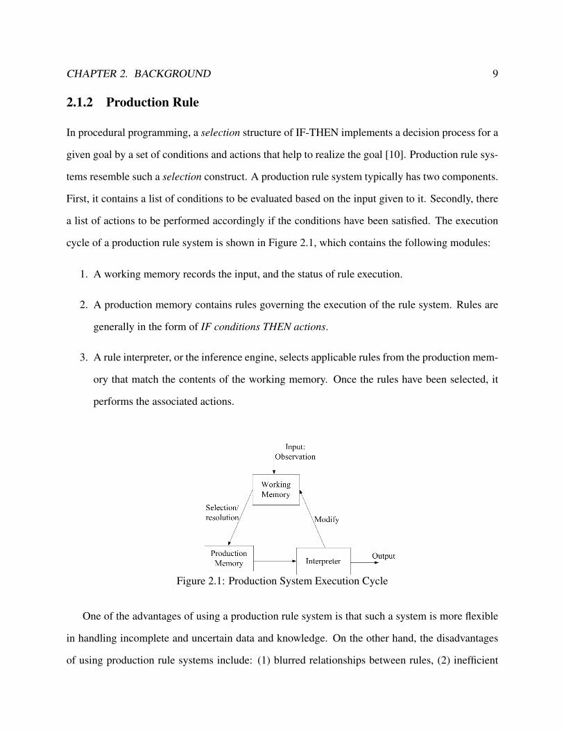
cycle of a production rule system is shown in Figure 2.1, which contains the following modules:
1. A working memory records the input, and the status of rule execution.
2. A production memory contains rules governing the execution of the rule system. Rules are
generally in the form of IF conditions THEN actions.
3. A rule interpreter, or the inference engine, selects applicable rules from the production mem-
ory that match the contents of the working memory. Once the rules have been selected, it
performs the associated actions.
Figure 2.1: Production System Execution Cycle
One of the advantages of using a production rule system is that such a system is more flexible
in handling incomplete and uncertain data and knowledge. On the other hand, the disadvantages
of using production rule systems include: (1) blurred relationships between rules, (2) inefficient

CHAPTER 2. BACKGROUND 10
rule searching strategy, especially in large pool of rules, and (3) inability to learn and evolve intel-
ligently.
2.1.3 Semantic Network
The origin of the Semantic Network lied in Aristotle’s associationism and reductionism, and later
became an attempt to describe the meaning of words and to give descriptions by associating sym-
bols in a given network. A semantic network is a graphical representation of information and
knowledge by interconnecting nodes and links. Nodes represent units of information, such as
concepts, predicates, properties, frames, features, and constraints. The links resemble inference
dependencies between nodes. An inference dependency provides semantic information, such as a
is a or subClassOf link, that describes the relationship between a pair of linked nodes. As a result,
class hierarchical and inheritance can be represented in semantic networks. Furthermore, practices
suggest that information and knowledge relevant to a specific node are typically clustered. This
resembles how human memory works in associating objects, and also enhances computational ef-
fectiveness [10]. Figure 2.2 shows an example of a semantic network. It represents that John is an
instance of the class STUDENT, while Semantic Web is an instance of the class COURSE. John, as
a student, enrolled in the course, Semantic Web.
Benefits of using the Semantic Network as a knowledge representation formalism include: first,
it provides efficient storage as technology and high-performance algorithms exist for network-
based data storage and manipulation. Secondly, inferencing about information and knowledge in
a semantic network reduces to traversing the network for which optimized algorithms also exist.
In addition, a semantic network can be transformed to an equivalent FOL representation, which
benefits from automatic Boolean Satisfiability Solvers [76] as means of logical deduction. A few
limitations of the Semantic Network exit, such as unable to express multiple inheritance cases,
disjunction, negation and quantification.

CHAPTER 2. BACKGROUND 11
Semantic Web
COURSE
is_A
John
enrolled
STUDENT
is_A
Figure 2.2: A Semantic Network Example
2.1.4 Frame
In 1975, Marvin Minsky proposed the theory of frames as a way to arrange knowledge. A frame
is presented as record-like data structure, which gathers all relevant information in one place for
handling situations. In other words, a frame contains descriptions of concepts and knowledge about
an entity, and its associations to other frames if any. Figure 2.3 shows a single frame of a student
instance identified by John. In this frame, Name, ID, LivedIn, enrolled, Admission Record, and
Student Frame
Name: JohnID: 123LivedIn: NYCenrolled:
Semantic WebObject-Oriented Programming
Admission RecordAcademic Advisor Links to other associated Frames
Figure 2.3: An Example of a Student Frame

CHAPTER 2. BACKGROUND 12
Academic Advisor are slots which are filled with values or links to other associated frames. For
instance, the a value, John, fills the Name slot, and the Admission Record slot is associated to other
frames.
There are a few limitations of representing knowledge in Frames. First, Frames are a general
methodology rather than a specific knowledge representation formalism. To an extremity, frames
can be used in an arbitrary manner, or ad hoc that lacks formal semantics. For instance, a frame for
a student and a frame for a person can have no common part, which is abnormal to most object-
oriented modeling approaches. Secondly, because of its ad hoc nature, there is no reasoning and
inference mechanism that can be justified.
2.1.5 Description Logic
Description Logic (DL) is closely related to Frames and Semantic Networks introduced in section
2.1.3 and 2.1.4 respectively. DL overcomes limitations of Frames and Semantic Networks to pro-
vide complete formal semantics and inference mechanisms. DL is based on Predicate Logic with
selective constructs that bear necessary expressive power for practical modeling purposes, and still
preserves good computational tractability.
In DL, facts are represented by descriptions, which contain properties or constraints individuals
need to satisfy in order to remain members or participants of the facts. A knowledge representation
system based on DL typically consists of two components: TBox and ABox. The TBox, or ter-
minology box, contains general knowledge in the form of concepts and roles about the knowledge
domain modeled. Concepts can be atomic or complex ones. An atomic concept is represented by
an unary predicate or logical expressions that contain only one free variable. A complex concept
is formed by atomic concepts with concept constructors, such as intersection or conjunction. As
an example, a concept, Woman is defined by the intersection of two atomic concepts, Person and
Female, and written as Woman ≡ Person u Female. Roles are binary predicates or logical ex-
pressions with two free variables. They can also be atomic or complex. For instance, hasChild

CHAPTER 2. BACKGROUND 13
is a complex role described by the union of two atomic roles, hasSon and hasDaughter. In com-
parison, an ABox contains assertional knowledge that is specific to individuals of the knowledge
domain modeled. Individuals are named constants, such as John. Assertional knowledge is subject
to change under different circumstances while the knowledge in TBox is not.
There are many language variants of Description Logic, and each provides different constructs
for levels of expressive power in exchange of computational tractability. The more expressive
power a DL language has, the less computational tractability it has. The Attribute Language, or
AL, is the minimal logic that contains a set of practically usable vocabulary. AL allows descrip-
tions of atomic concepts, atomic roles, atomic negation, value restrictions, and limited existential
quantification. It can be further extended by adding new constructs to enable more expressive
power. Table 2.1 shows symbolic names of possible extensions to AL logic. The name of a new
logic is formed from the string AL[U ][E ][N ][C]. For instance, the logic ALC is the AL logic ex-
tended with the negation of an arbitrary concept. ALC is also called S due to its relationship to
propositional modal logic S4m [39, 61]. Further extending the logic (S) to include role hierar-
chy (H), nominals (O), inverse roles (I), number restrictions (N ), and concrete domains results
the logic SHOIN (D) on which OWL-DL is based. OWL-Lite, OWL-DL, and OWL-Full [50]
are three variants of the Web Ontology Language, OWL, with increasing expressive power and
computational overhead.
Name Syntax NoteU C tD Union of Two ConceptsE ∃R.C Full Existential QuantificationN ≥ nR Number Restriction
≤ nRC ¬C Negation of an Arbitrary Concepts
Table 2.1: Extensions to AL logic
The main inference task over concept and role expressions in DL is subsumption. Given two
concepts C and D, if the concept described by D is more general than another denoted by C, D

CHAPTER 2. BACKGROUND 14
subsums C and write C ⊆ D. Other inference tasks in DL include satisfiability, instance checking,
equivalence checking, and the retrieval of a set of individuals that satisfy a concept description.
2.2 The Semantic Web
The Semantic Web is a collaborative project envisioned by Tim Berners-Lee [12], the inventor
of the World Wide Web. It aims at achieving a linked-data medium for machine-processable in-
formation exchange on the World Wide Web. The Semantic Web provides additional metadata
specification, so web contents or resources can be annotated with metadata and also linked. The
Semantic Web technologies enable users to create vocabularies and data stores, use and represent
data and knowledge, and reason about meanings of data and knowledge. The linked-data is facil-
itated by technologies such as Resource Description Framework (RDF), SPARQL, Web Ontology
Language (OWL), etc.
The efforts on the development of the Semantic Web technologies led by W3C have popu-
larized ontology, knowledge representation, and reasoning for machine processing. Ontology is
the study or concern about what kinds of things exist, what entities or things there are in the uni-
verse. In Computer Science, ontology is a model of concepts and relationships among them. The
most popular definition of ontology cited is due to Gruber. Gruber [29] defined an ontology as
the specification of conceptualizations used to help programs and human share knowledge. Such
a conceptualization relies on the knowledge about the world in terms of entities and relationships,
which are similar to the Entity-Relationship data model used in relational database modeling. Main
components in an ontology are concepts, relations, instances, and axioms, briefly described as fol-
lows:
• Concepts are considered invariants. That is, things do not change in reality. A concept
represents a set of entities, or a class, and may have properties, such as subclass or super-
class. Furthermore, a concept is either a primitive concept or a defined concept. A primitive

CHAPTER 2. BACKGROUND 15
concept is fundamental and reflects necessary conditions for being a member of that con-
cept, whereas a defined concept is derived by joining primitive concepts and reflects both
necessary and sufficient conditions for being a member of that derived concept.
• Relations describe the relationships between concepts or properties of concepts.
• Instances are existing things represented by a concept via membership. For instance, John
as an individual is an instance of the concept Student.
• Axioms are rules to constrain properties or memberships of classes or instances.
The World Wide Web Consortium (W3C) has established a set of recommended standards for
representing data and knowledge in ways that machines can process. Resource Description Frame-
work (RDF), Web Ontology Language (OWL), and XML based languages have been developed.
Specifically, they support concept descriptions of data and knowledge in different styles of syntax,
notations, and serialization formats. For RDF, we present its formal definitions in Appendix A and
how it is used in the following section in this chapter. Web Ontology Language (OWL) is based
on Description Logic and provides more expressive power than RDF does. For the scope of this
research, we will skip discussions of OWL.
2.3 RDF Basics
Resource Description Framework (RDF) [21] is a graph-based data model. Its basic form is a
triple: (subject, predicate, object) that asserts a named property for a subject. For instance, (John,
enrolled, SW) is a triple that asserts that John enrolled in a course SW, or the Semantic Web. Each
component in a triple is a RDF resource identified by International Resource Identifier (IRI) [21]
that conforms to RFC3987 [22], or a local existential variable for a blank node. The predicate
logically relates a subject resource to an object resource. A subject and an object of a RDF triple
CHAPTER 2. BACKGROUND 16
are visualized as vertices while a predicate is visualized as an edge. A set of logically related RDF
triples constitutes a RDF graph.
RDF is formed by layered sets of pre-defined vocabularies, such as RDF vocabulary or RDF
Schema vocabulary. These vocabularies provide different levels of expressive power. RDF vocab-
ulary, or rdfV, includes a typing predicate and a superclass of all RDF properties. RDF Schema
[16], or RDFS, further extends RDF, as a semantic extension, to allow descriptions of classes, their
relationships, and properties, which can be arranged in a hierarchy of classes or properties. In
addition, certain types of inferencing, such as class membership and subclass hierarchy, are sup-
ported in RDF Schema by stating the classes to which the subject and the object of a property must
belong.
The formal semantics of the Semantic Web layered stack is defined accordingly for each se-
mantic extension. Model-theoretic semantics is used to define an interpretation model for each
semantic extension. Defining an interpretation model also characterizes an entailment regime. For
instance, two entailment patterns are defined for rdfV, while thirteen patterns are defined for RDF
Schema [36]. RDF entailment and inference definitions can be found in Appendix A.
SPARQL Protocol and RDF Query Language (SPARQL) [58] and its newer version SPARQL1.1
[32] are the main query language for RDF and RDFS triple databases. From now on when we say
SPARQL, it refers to its latest version SPARQL 1.1. SPARQL has a similar syntax form to SQL,
but it is specifically tailored for graphs. SPARQL provides graph pattern specifications and a SE-
LECT construct, among others, to retrieve matched graph segments from a RDF graph. Definitions
and query examples of SPARQL is detailed in Appendix A.
In the remainder of this chapter, we focus on RDF namespace, notations, and a running example
for illustrating how RDF and RDFS are used. Moreover, RDF reification will be discussed as
it is an important aspect that serves as a foundation for our survey of temporal data models of
the Semantic Web that will be presented in Chapter 3. For RDF, its formal model definitions,
semantics, entailment patterns, and the query language, SPARQL are given in Appendix A.

CHAPTER 2. BACKGROUND 17
As a starting example, consider the facts given in Table 2.2: John enrolled in the Semantic Web
course, or SW, and he lived in NYC.
Name enrolled livedIn
John SW NYC
Table 2.2: Person Relation
A transformation of Table 2.2 allows us to identify John, SW, and NYC as resources, and
further model these facts as two RDF triples: (John, enrolled, SW) and (John, livedIn, NYC).
These two triples are presented as a RDF graph shown in Figure 2.4.
ex:John
ex:SWex:enrolled
ex:NYC
ex:livedIn
Figure 2.4: Person Relation Transformed to a RDF Graph
2.4 RDF Namespace and Notation
To encode a RDF graph, W3C recommends serializing it into a verbose XML or a compact syntax,
such as Notation 3 (N3) [11], Turtle [9], or N-Triples [8], etc. These three variations of syntax are
closely related in that N3 is the superset of Turtle and N-Triples. That is: N-Triples ⊂ Turtle ⊂
N3. In this thesis, graph-based representations of examples are used for illustrating the standard
RDF model, and our proposed Valid Time RDF, which will be defined in Chapter 4. For a RDF
graph presentation, such as the graph in Figure 2.4, an oval denotes a RDF resource or a literal
as a subject or an object. A directed link represents a predicate. When a literal value is used, it

CHAPTER 2. BACKGROUND 18
is double quoted and annotated with a data type or a language tag. The RDF graph illustrated in
Figure 2.4 will be used as the RDF running example to illustrate aspects of RDF in the remainder
of this chapter and also in Appendix A, which provides detailed definitions of RDF vocabularies,
their semantics, and inference patterns.
When necessary, we also use the line-based Turtle syntax of [9] for presenting RDF triples and
graphs. A triple written in Turtle syntax has the form shown in Figure 2.5. The angled bracket
pair in each resource encloses a full IRI. When a prefix is appropriately declared, a full IRI may be
shortened by carrying the prefix and without the angled brackets.
<subject> <predicate> <object>.
Figure 2.5: Line-based Turtle Syntax [9]
For instance, Figure 2.6 shows the serialization of the RDF graph of Figure 2.4 in Turtle syntax
[9], and Figure 2.7 shows the same example in RDF/XML serialization.
PREFIX ex: <http://example.org/RDF-SW#>.
ex:John ex:enrolled ex:SW.
ex:John ex:livedIn ex:NYC.
Figure 2.6: RDF Running Example in Turtle Syntax
The namespace and prefix taken from [1, 20], shown in Figure 2.8, will be used as common no-
tations in all RDF modeling and query examples in this chapter and Appendix A, unless otherwise
specified.
The prefix rdf: and rdfs: refer to the namespace of RDF vocabulary and RDF schema respec-
tively. Our running example is under a base ontology identified by http://example.org/RDF-SW.
We use ex: as its prefix. In the standard RDF model, an IRI may contain a fragment identifier, sep-
arated by the symbol # [21], that denotes an additional part of the primary resource. For instance,

CHAPTER 2. BACKGROUND 19
<?xml version="1.0"?><rdf:RDF xmlns="http://example.org/RDF-SW#"xml:base="http://example.org/RDF-SW"xmlns:RDF-SW="http://example.org/RDF-SW#"xmlns:rdf="http://www.w3.org/1999/02/22-rdf-syntax-ns#"xmlns:owl="http://www.w3.org/2002/07/owl#"xmlns:xml="http://www.w3.org/XML/1998/namespace"xmlns:xsd="http://www.w3.org/2001/XMLSchema#"xmlns:rdfs="http://www.w3.org/2000/01/rdf-schema#"><owl:Ontology rdf:about="http://example.org/RDF-SW"/><owl:ObjectProperty rdf:about="http://example.org/RDF-SW#enrolled"/><owl:ObjectProperty rdf:about="http://example.org/RDF-SW#livedIn"/><owl:NamedIndividual rdf:about="http://example.org/RDF-SW#John"><enrolled rdf:resource="http://example.org/RDF-SW#SW"/><livedIn rdf:resource="http://example.org/RDF-SW#NYC"/></owl:NamedIndividual><owl:NamedIndividual rdf:about="http://example.org/RDF-SW#NYC"/><owl:NamedIndividual rdf:about="http://example.org/RDF-SW#SW"/></rdf:RDF>
<!-- Generated by the OWL API (version 4.2.8.20170104-2310)https://github.com/owlcs/owlapi -->
Figure 2.7: RDF Running Example in RDF/XML
@PREFIX xsd: <http://www.w3.org/2001/XMLSchema#> .@PREFIX rdf: <http://www.w3.org/1999/02/22-rdf-syntax-ns#> .@PREFIX rdfs: <http://www.w3.org/2000/01/rdf-schema#> .@PREFIX owl: <http://www.w3.org/2002/07/owl#> .@PREFIX ex: <http://example.org/RDF-SW#> .
Figure 2.8: Prefix for RDF Examples
http://example.org/RDF-SW#John contains a fragment identifier ‘John’that is under the primary
resource denoted by http://example.org/RDF-SW.
We have prepared formal definitions of RDF syntax, semantics, entailment patterns, and SPARQL
query examples in Appendix A for reference.
2.5 RDF Reification
The verb reify originates from res in Latin, meaning to thingify or to convert into a concrete thing. It
is commonly used in different disciplines. For instance, in First Order Logic, reification generally

CHAPTER 2. BACKGROUND 20
refers to the use of terms to express concepts that are normally represented using predicates [27]. In
other words, it allows making an assertion about a predicate. RDF is confined to binary predicates;
hence reification is needed to represent higher-arity predicates. A RDF triple makes an assertion
about a subject and an object. We can consider it as an atomic statement. When we want to make
another assertion about an atomic statement, we need a new construct in RDF. That is reification.
A reification process starts by making a given statement bind to a new identifiable resource (i.e.,
an identifier is used to represent the statement) which acts as a proxy for the statement. The proxy
then can further be used to assert properties on behalf of the statement.
Consider the facts given in Table 2.3. John enrolled in the Semantic Web course when he
lived in NYC, and a time interval is associated with facts about John. Clearly, this statement
asserts several facts and can not be expressed in one RDF triple. For instance, a binary predicate
enrolled(John, SW) represents part of this fact. If the predicate enrolled is reified, it becomes a
new term that can be used consequently as a component in other assertions. We explain the two
forms of reification by an example.
Name enrolled livedIn hasDate
John SW NYC 2/1/2016-5/31/2016
Table 2.3: Person Relation with Temporal Information
There are two types of reification in RDF: implicit reification and explicit reification. We il-
lustrate both forms of reification by using the facts given in Person relation of Table 2.3, which
represents a person whose name is John. For simplicity, we also use the term John as an identi-
fier. This individual enrolled in SW, lived in NYC, and had a validity interval 2/1/2016-5/31/2016.
Person(John, SW, NYC, 2/1/2016-5/31/2016) is a 4-ary predicate that represents the relation given
in Person table. Obviously, RDF can not represent it directly, so it needs to be broken into several
triples by using reification. Implicit reification allows defining binary predicates shown in Figure
2.9. Obviously, implicit reification breaks any n-ary relationships into several binary relationships.

CHAPTER 2. BACKGROUND 21
This is similar to representing a n-ary relationship in Entity Relationship Data models into corre-
sponding binary relationships.
enrolled(John, SW)livedIn(John, NYC)hasDate(John, 2/1/2016-5/31/2016)
Figure 2.9: Binary Predicates for Person Relation
All of these predicates can directly be represented in RDF. enrolled and livedIN predicates are
clear; however the last predicate hasDate(John, 2/1/2016-5/31/2016) asserts that John has a date
2/1/2016-5/31/2016. It is not clear whether it is for enrolled or livedIn, or both, or something
else. Resolving this ambiguity requires explicit reification that is also provided in RDF, which are
the vocabularies: rdf:Statement, rdf:subject, rdf:predicate, and rdf:object defined in Appendix A.2.
Considering that the date value 2/1/2016-5/31/2016 actually applies to John’s enrollment in SW,
this fact is reified as given in Figure 2.10.
In explicit RDF reification process, a triple is instantiated as a new resource that belongs to
the class rdf:Statement. According to RDF specification, the new resource required in reification
can be written as a blank node or identified by an IRI. In the latter case, such an IRI does not
represent any concrete realization of a triple or resource. The original triple can then be associated
with additional properties as if it is a standard resource. Figure 2.10 depicts the reification of
a simple triple (ex:John, ex:enrolled, ex:SW). First a new identifier ex:stmt1 is defined . This
identifier represents the triple, (ex:John, ex:enrolled, ex:SW), which is further augmented by meta
properties. Hence, components of the original triple become objects of special meta properties,
including rdf:subject, rdf:predicate and rdf:object. The new resource ex:stmt1 can be described
by additional properties, such as the occurring time (2/1/2016 to 5/31/2016), place, certainty or
provenance.
According to RDF specification, ’the reification of a triple does not entail the triple, and is not
entailed by it’ [36]. However, from the reification in Figure 2.10, there is an entailment pattern

CHAPTER 2. BACKGROUND 22
ex:stmt1
rdf:Statementrdf:type
ex:Johnrdf:subject
ex:enrolledrdf:predicate
ex:SW
rdf:object
Figure 2.10: RDF Reification of (ex:John, ex:enrolled, ex:SW)
to infer the original triple of (John, enrolled, SW). Since RDF specification does not constrain the
semantics of standard reification, it is the user’s decision to accept the entailment pattern or not.
Moreover, reification also suffers from the proliferation of extra objects and triples that are
needed for representing higher order relations. That is, to reify (John, enrolled, SW), four addi-
tional triples are needed before additional facts can be added. As a result, the graph size increases.
And even worse, the reified graph makes queries more difficult to write as we will see it in an
example later.
For the user’s convenience, two presentations of RDF graphs are commonly used in the litera-
ture. Figure 2.11(a) includes the original triple instead of converting the predicate :enrolled to an
object. In contrast, Figure 2.11(b) uses a node connecting to an edge instead of another node. This
treatment is a violation of the general definition of graphs, and common graph-based operations
can not be applied directly.
As we shall see in the next chapter, proposals of temporal extensions to RDF reported in the
literatures mostly use RDF reification explicitly or implicitly.

CHAPTER 2. BACKGROUND 23
ex:SW
ex:John
ex:stmt1
ex:enrolled
ex:enrolled
rdf:predicate rdf:object
rdf:subject
(a)
ex:SW
ex:John
ex:stmt1ex:enrolled rdf:predicate
rdf:object
rdf:subject
(b)
Figure 2.11: Two Common Graph Representations of RDF Reification for (ex:John, ex:enrolled,ex:SW)

Chapter 3
Survey of Temporal Extensions to RDF
3.1 The Running Example and Namespace
In this chapter, we survey temporal data models of the Semantic Web reported in the literature.
This survey is also based on our previous study in [72]. We examine the characteristics of each
temporal model and develop a taxonomy to categorize them into two groups: explicit reification-
based and implicit reification-based. Explicit reification-based temporal models involve the use
of standard RDF reification. In comparison, temporal models in implicit reification group employ
some mechanism to identify a concept, a triple, a relationship or a graph. This group is further cate-
gorized into three subgroups: (1) Instantiating-Identifying Concept/Relationship, (2) Relationship
Entity Conversion, and (3) Named Graphs.
For each model, we consider core model components, extensions to RDF/RDFS vocabularies,
SPARQL query support and special features, if any.
Running Example and Query The data in Table 2.3 is used for illustrating each temporal model.
A simple RDF triple, (John, enrolled, SW), asserts the fact about an individual Student John and his
enrollment in a Semantic Web course between 2/1/2016 and 5/31/2016. The predicate enrolled re-
24
CHAPTER 3. SURVEY OF TEMPORAL EXTENSIONS TO RDF 25
lates a Student instance to a Class instance (i.e., as domain and range respectively). Furthermore, a
semi-closed interval [2/1/2016, 5/31/2016) needs to be associated with this triple. John may enroll
in other courses over time. Hence, it is conceivable to have another triple: (John, enrolled, OOP)
making another assertion about his enrollment in other time, such as [8/31/2016, 12/22/2016).
The query ”retrieve the valid time when John enrolled in the Semantic Web course” will also
be used as a running query to illustrate how a query is expressed in each temporal model and its
version of SPARQL [32].
Namespace and Prefixes The prefixes and namespace defined in section 2.4 remain in use
as a common notation for all examples unless otherwise specified. Additional prefixes are needed,
and we combine them as follows:
@PREFIX xsd: <http://www.w3.org/2001/XMLSchema#>.
@PREFIX rdf: <http://www.w3.org/1999/02/22-rdf-syntax-ns#>.
@PREFIX rdfs: <http://www.w3.org/2000/01/rdf-schema#>.
@PREFIX owl: <http://www.w3.org/2002/07/owl#>.
@PREFIX owlTime: <http://www.w3.org/2006/time#>.
@PREFIX : <http://example.org/Temporal-SW#>.
The base ontology of the running example for the survey has a Namespace– http://example.org/Temporal-
SW#, and we use : (colon) as its prefix.
3.2 Time Domain
W3C recommended OWL-Time ontology [37] as a standard for definitions of temporal entities:
instant and interval, and properties, such as before, after or equals for instants or intervals. Some
CHAPTER 3. SURVEY OF TEMPORAL EXTENSIONS TO RDF 26
of the proposed temporal models use OWL-Time ontology, whereas others include their own defi-
nition of time, such as using natural numbers. For the scope of this thesis, time domain is defined
as follows and will be used in this survey and also in our proposed VTRDF in Chapter 4.
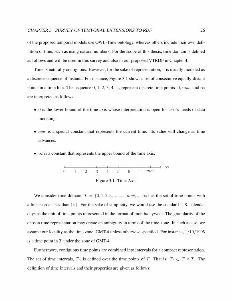
Time is naturally contiguous. However, for the sake of representation, it is usually modeled as
a discrete sequence of instants. For instance, Figure 3.1 shows a set of consecutive equally-distant
points in a time line. The sequence 0, 1, 2, 3, 4, ..., represent discrete time points. 0, now, and∞
are interpreted as follows:
• 0 is the lower bound of the time axis whose interpretation is open for user’s needs of data
modeling.
• now is a special constant that represents the current time. Its value will change as time
advances.
• ∞ is a constant that represents the upper bound of the time axis.
0 1 2 3 4 5 6.... now
∞
Figure 3.1: Time Axis
We consider time domain, T = {0, 1, 2, 3, ......, ...now, ...,∞} as the set of time points with
a linear order less-than (<). For the sake of simplicity, we would use the standard U.S. calendar
days as the unit of time points represented in the format of month/day/year. The granularity of the
chosen time representation may create an ambiguity in terms of the time zone. In such a case, we
assume our locality as the time zone, GMT-4 unless otherwise specified. For instance, 1/10/1995
is a time point in T under the zone of GMT-4.
Furthermore, contiguous time points are combined into intervals for a compact representation.
The set of time intervals, TI , is defined over the time points of T . That is: TI ⊂ T × T . The
definition of time intervals and their properties are given as follows:

CHAPTER 3. SURVEY OF TEMPORAL EXTENSIONS TO RDF 27
• Let [l, u) be a time interval that contains a finite set of consecutive time points between l and
u. l is the beginning time point or lower bound of the interval. u is the end time point or
upper bound. The set of time intervals, TI , is:
TI = {[l, u)|l ∈ T ∧ u ∈ T ∧ l < u} (3.2.1)
In this case, each interval [l, u) is closed at the beginning and open at the end. A time
interval may be closed at both ends, such as [l, u]. In the remainder of the paper, we may use
an identifier i and an explicit representation [l, u) interchangeably to reference an interval.
• Two disjoint intervals [l, u) and [l′, u′) share no common time points, or [l, u) ∩ [l′, u′) = ∅.
Otherwise, they overlap or [l, u) ∩ [l′, u′) 6= ∅.
• Two intervals [l1, u1) and [l2, u2) are adjacent if l2 = u1 or l1 = u2.
• Set theoretic operations, such as union, intersection, and difference can be defined on inter-
vals. Nevertheless, intervals are not closed under set theoretic operations.
• When the closure property is required, temporal elements [26] can be used in place of in-
tervals. A temporal element is a finite union of disjoint and non-adjacent intervals. For
instance, the set {[1/10/1985, 1/10/2005), [2/1/2016, 5/31/2016)} is a temporal element.
A set of temporal elements are closed under set theoretic operations.
3.3 Explicit Reification Based Temporal Models
One of the early and formal extensions of RDF to handle temporality is Temporal RDF [30]. Later
enhancements are introduced to this extension, such as [19, 41, 59]. In the following, we review
Temporal RDF and its enhanced versions.

CHAPTER 3. SURVEY OF TEMPORAL EXTENSIONS TO RDF 28
Temporal RDF In Temporal RDF [30], each triple is timestamped with a time instant or an
interval. Timestamping is achieved by using standard RDF definitions and an internal time domain
that includes temporal property specifications, such as temporal, instant, interval, initial and final.
A Temporal RDF triple is in the form of (s, p, o)[T] and visualized as a temporal RDF graph given
in Figure 3.2. ”:stmt1” and ”:temporal#1” are ground nodes that substitute blank nodes, which are
used as subjects in the original work for reification.
:SW
:John
:stmt1 :temporal#1 :i1
2/1/2016
5/31/2016
:enrolled:temporal :interval :initial
:final
rdf:predicate
rdf:object
rdf:subject
Figure 3.2: Temporal RDF
In Figure 3.2, the triple (John, enrolled, SW) is reified by :stmt1 of rdf:Statement class. :stmt1,
is further associated with a temporal entity :temporal#1 and then an interval :i1. :i1 is the valid
time interval of the triple which has its begin and finish time instants ”2/1/2016” and ”5/31/2016”
respectively, whereas natural numbers are used as time instants in the original work. This temporal
fact is therefore represented by seven RDF triples in the case of time interval and by six triples in
the case of time instant.
The semantics of a Temporal RDF graph [30] is provided in terms of non-temporal RDF and
RDFS graphs. Temporal entailment is defined based on the closure of temporal and non-temporal
graphs. Specifically, a temporal graph G1 entails G2, denoted by G1 |= G2, if and only temporal
closure ofG1 entailsG2. Furthermore, a deductive inference rule system for Temporal RDF graphs

CHAPTER 3. SURVEY OF TEMPORAL EXTENSIONS TO RDF 29
is outlined. Temporal rules are defined to equate an interval and a instant version of temporal
graphs.
A query language proposed for Temporal RDF graphs is provided in SQWRL-like [54] rule
form. The running example query can be expressed conceptually as follows:
(:X, :interval, ?Y), (?Y, :initial, ?ti), (?Y, :final, ?tf)
<-- (:John, :enrolled, :SW):[?ti, ?tf].
Rewriting the above working query in SPARQL results in the following:
SELECT ?Y ?ti ?tf
WHERE { :John :enrolled :SW.
?X rdf:type rdf:Statement.
?X rdf:subject :John.
?X rdf:predicate :enrolled.
?X rdf:object :SW.
?X :interval ?Y.
?Y :initial ?ti.
?Y :final ?tf.
}
In this query, presence of the original triple (John, enrolled, SW) is assumed. Nevertheless, the
query result preserves it even if this assumption is dropped. Query processing and semantics are
also defined as a temporal tableau similar to a language presented in [31]. The complexity of query
processing of the rule-like form above is briefly explained. Moreover, the authors conclude that
the additional time dimension in their proposal does not add to the complexity of query answering.
In other words, Temporal RDF model is still NP complete in query processing.

CHAPTER 3. SURVEY OF TEMPORAL EXTENSIONS TO RDF 30
Enhanced Temporal RDF The temporal RDF model [30] is enhanced by allowing anonymous
timestamp [19]. A temporal triple is represented in a similar form, (s, p, o):[X] where X is an
anonymous timestamp, i.e., unknown time. General temporal graphs are defined as temporal
graphs with known or anonymous timestamps. The t-ground general temporal graph is defined as
one that does not contain anonymous timestamps.
The semantics of general temporal graphs is given similar to Temporal RDF semantics devel-
oped in [30] and it includes an additional slice closure of general temporal graphs. Slice closure
of a general temporal graph is computed by a non-temporal closure of snapshot graphs for each
time point. The complexity of evaluating entailment for general Temporal RDF graphs is shown to
be NP-complete. Query language for the general Temporal RDF is similar to the example shown
above for Temporal RDF.
C-Temporal Graph Temporal RDF model [30] is further extended to include temporal con-
straints and reasoning [41]. A C-Temporal Graph is a pair C = (G,Σ), where G is a graph with
temporal triples, and Σ is a set of temporal constraints over time intervals of G. Temporal blanks
are introduced, and time variables in Temporal RDF [30] are allowed. This treatment is the same
as the anonymous timestamp [19]. As an example, a student went to high school at an unknown
time T1, and later he went to college at some other unknown time, T2. These facts are represented
as two Temporal RDF triples with the timestamp T1 and T2 as time variables respectively. To
preserve a proper temporal order, a constraint, T2 > T1, is enforced in the model. Entailment of
a C-Temporal graph can be reduced to finding mappings to the closed version of temporal slice
closure defined in [19]. Additionally, query processing for C-Temporal graphs also reduces to
matching the query pattern and the closed graphs.
tRDF for Indeterminate Triples The tRDF model [59] is based on the Temporal RDF proposed
earlier in [30, 19]. tRDF particularly supports another type of anonymous timestamp in indeter-

CHAPTER 3. SURVEY OF TEMPORAL EXTENSIONS TO RDF 31
minate triples. A determinate triple (s, p, o)[T] represents a relationship p between s and o that
holds at every time point in the time interval T. In contrast, an indeterminate triple (s, p:[n:T], o)
represents that the relationship holds at most n distinct time points in T. A tRDF graph includes
indeterminate temporal triples. In addition, the concept of normalizing a tRDF graph is defined
in order to preserve good properties of the tRDF model. Normalizing tRDF employs the notion
of value-equivalent-tuples from temporal databases [42]. Two tRDF triples are value-equivalent if
their non-temporal parts are identical. As an example, suppose John actually enrolled in Semantic
Web class twice: (John, enrolled, SW)[T1] and (John, enrolled, SW)[T2]. Instead of storing two
value-equivalent triples, coalescence is applied to merge overlapping or connecting intervals into a
single cumulative interval, i.e., T1⋃T2. The consolidated interval can then be used as the times-
tamp of a single representative triple (John, enrolled, SW){T1⋃T2}. As a result, a normalized
tRDF graph G entails each one of the coalesced tRDF graphs.
Indexing structure, tGRIN, is proposed to improve the performance of tRDF triple storage
in query evaluation. A tGRIN index is a balanced tree structure that stores close graph vertices
together in the same index node. The closeness of two resources x and y is determined by a distance
metric that combines general graph distance, dG(x, y), and temporal graph distance, dT (x, y), by a
k-norm function, [dG(x, y)k + dT (x, y)k]1/k [59]. Experiments show that tGRIN is a better match
for tRDF queries than the use of standard B-tree used in traditional relational databases.
The formal semantics and querying tRDF are based on equivalent models developed in Tempo-
ral RDF [30, 19]. Additional semantic conditions are also needed to interpret indeterminate triples
and queries.
Generalized RDF Annotation In [79], a generalized framework for representing and reasoning
annotated RDFS is proposed. This model is based on the works of annotated RDF [71] and its
query language, AnQL [44]. Annotated RDFS is based on the logic programming, and has an
abstract form of triples: (s,p,o)[T]. The annotation domain could be temporal, fuzzy, their com-
CHAPTER 3. SURVEY OF TEMPORAL EXTENSIONS TO RDF 32
bination, or others. It is defined as an algebraic structure: D = {L,�,∧,∨,⊗ ⇒,⊥,>} where
elements in L are annotation terms. For instance, L=[0,1] is for a fuzzy domain while L=[T] id
for a temporal domain. The top>, bottom⊥, order �, meet operator ∧, join operator ∨ and t-norm
⊗ are used for constructing the annotation domain and its inference patterns. The t-norm ⊗ is
used to model the conjunction of information. For instance, from (a, rdfs:subClassOf, b):I and (b,
rdfs:subClassOf, c):I’, infer (a, rdfs:subClassOf, c):I ⊗ I’. For the temporal case, ⊗ is overloaded
to represent the intersection of time intervals. Multiple annotation domains may be combined using
the generalized framework. A complex domain D can be constructed from individual annotation
domains: D = D1 ×D2 × ....×Dn = {L,�,⊗,⊥,>}. The model is also augmented by a set of
inference rules for annotated RDFS.
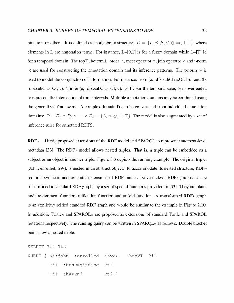
RDF? Hartig proposed extensions of the RDF model and SPARQL to represent statement-level
metadata [33]. The RDF? model allows nested triples. That is, a triple can be embedded as a
subject or an object in another triple. Figure 3.3 depicts the running example. The original triple,
(John, enrolled, SW), is nested in an abstract object. To accommodate its nested structure, RDF?
requires syntactic and semantic extensions of RDF model. Nevertheless, RDF? graphs can be
transformed to standard RDF graphs by a set of special functions provided in [33]. They are blank
node assignment function, reification function and unfold function. A transformed RDF? graph
is an explicitly reified standard RDF graph and would be similar to the example in Figure 2.10.
In addition, Turtle? and SPARQL? are proposed as extensions of standard Turtle and SPARQL
notations respectively. The running query can be written in SPARQL? as follows. Double bracket
pairs show a nested triple:
SELECT ?t1 ?t2
WHERE { <<:john :enrolled :sw>> :hasVT ?i1.
?i1 :hasBeginning ?t1.
?i1 :hasEnd ?t2.}

CHAPTER 3. SURVEY OF TEMPORAL EXTENSIONS TO RDF 33
:john
:sw
:enrolled
:i1:hasVT
2/1/2016 5/31/2016
:hasBeginning :hasEnd
Figure 3.3: RDF?
YAGO 2 The original YAGO Knowledge Base [65] is constructed automatically from articles
on Wikipedia. Each simple article on Wikipedia belongs to a article category, and mainly contains
a lead section, a content body, appendices and bottom notes [3]. An article becomes an entity in
YAGO. Article categories on Wikipedia provide the typing information for it. Th typing informa-
tion is linked to the taxonomy of WordNet [38]. In YAGO, each fact is represented by a triple, (s,
p, o). Each fact is also reified, so a triple identifier is assigned. This effectively results a quintuple:
(id, s, p, o).
YAGO2 is the new version of YAGO. YAGO2 employs an extensible extraction architecture
that is based on declarative rules, whereas YAGO’s extraction rules are hard-wired to the source
code [38]. In addition, YAGO2 incorporate both temporal and spatial dimensions to the knowledge
base. For the temporal dimension, yagoDate is the main data type that denotes time points in days.
A time interval can be represented by two time points with a pair of relations, such as occursSince
and OccursUntil [38]. Entity time and Fact time to denotes its existence in time, and the event
period respectively. The running example can be represented similarly to Temporal RDF of Figure
3.2

CHAPTER 3. SURVEY OF TEMPORAL EXTENSIONS TO RDF 34
3.4 Implicit Reification Based Temporal Models
In general, implicit reification based models use different types of abstraction for handling reifi-
cation. They do not employ reification vocabularies of RDF specifications. Two subcategories
follow.
3.4.1 Instantiating-Identifying Concept/Relationship (IIR)
In IIR models, a concept or relationship is reified and further temporalized. Either such relationship
is abstracted as a new object, or a concept is viewed as four dimensional and instantiated to have
temporal extents. Singleton Property converts each relationship to be universally unique. 4D
fluents use concepts that view each resource as a perdurant. Fluents represent properties that change
over time.
Singleton Property Nguyen et al. propose the concept of singleton property for representing
and querying meta knowledge in [52]. This approach recognizes each RDF triple as an unique
relationship and introduces multiple contextual instances to it as needed. Given a relationship
between two objects under a context, a singleton property is introduced to denote the relationship
instance with a specific context, such as temporality, provenance, etc. In other words, a singleton
property is an instance of a given relationship used to assert the context property values. Figure
3.4 shows the running example in singleton property approach.
:John :SW:enrolled 1
:enrolled 1:enrolled :i1 2/1/2016
5/31/2016
:hasBeginningrdf:singletonPropertyOf
:hasEnd
:hasVT
Figure 3.4: Singleton Property

CHAPTER 3. SURVEY OF TEMPORAL EXTENSIONS TO RDF 35
The unique property :enrolled 1 in Figure 3.4 is an instantiation of the generic :enrolled by the
predicate, rdf:singletonPropertyOf. It is then used for asserting the relationship between John and
the class SW. The temporal context is therefore asserted by (:enrolled 1, :hasVT, :i1).
The formal semantics of the singleton property is derived from the standard RDF and RDFS
semantics with the additional semantics extension for the vocabulary rdf:singletonPropertyOf. The
singleton property gives rises to three cases of query patterns: data, metadata and mixed patterns
which SPARQL supports. The running example query belongs to the metadata pattern and can be
written in SPARQL as follows:
SELECT ?ti ?tf
WHERE { ?p rdf:singletonPropertyOf :enrolled.
:john ?p :sw.
?p :hasVT ?i1.
?i1 :hasBeginning ?ti.
?i1 :hasEnd ?tf.
}
4D Fluents Welty et al. proposed 4D Fluents model for representing time-varying relationships
in OWL [73]. This model employs 4D view and Fluent. Haynes introduced four dimensional view
or perdurantist view into Computer Science in his seminal work [35]. Perdurantism is a philo-
sophical theory of persistence and identity [34], and it is closely related to four dimensionalism. In
the four dimensional view, an object that persists through time has distinct temporal parts at every
time instant through its existence in time. Furthermore, each persisting object can be considered a
four dimensional spacetime worm that stretches across space-time. Slicing the worm at a specific
time interval or instant of the time dimension yields a temporal part. A Temporal part is also called
a time slice in other literature [49]. The slicing produces entity-at-a-time. In contrast, three di-
mensional view considers that an object is wholly present or endures through its existence in time.

CHAPTER 3. SURVEY OF TEMPORAL EXTENSIONS TO RDF 36
Therefore there are no temporal parts.
Fluent is a component of Situational Calculus which is a logical language for representing
change. McCarthy first introduced Situational Calculus [46, 48]. It concerns situations, actions
and fluents in a dynamic domain. Actions make the domain change from one situation to another.
Fluents are situation-dependent functions for describing the effects of actions.
In 4D Fluents model, fluents are properties that change over time [73]. These properties are
special cases in that both the domain and range of them are temporal parts of the corresponding
entities. TemporalPart is the main class for converting regular entities to 4D spacetime worm ones.
OWL-Time ontology of [37] is used as time domain in 4D Fluents model. Particularly, a class
TimeInterval derived from the equivalent class of OWL-Time is used for all temporal terms.
Several object and fluents properties are listed in Table 3.1. Figure 3.5 represents running
example in 4D Fluents model.
Object Property Domain Range:fluentProperty :TemporalPart :TemporalPart:temporalExtent :TemporalPart :TimeInterval:temporalPartOf :TemporalPart complementOf(:TimeInterval)
Table 3.1: Object Property of 4D Fluents Ontology
:John
:SW
:John@i1
:SW@i1
:temporalPartOf
:temporalPartOf
:enrolled
:i1 2/1/2016
5/31/2016
:temporalExt
:temporalExt
:hasBeginning
:hasEnd
Figure 3.5: 4D Fluents
In Figure 3.5, individuals :John and :SW are two 4D entities. Each entity has temporal parts,
:John@i1 and :SW@i1 respectively. The property :enrolled is transformed to a fluent whose do-

CHAPTER 3. SURVEY OF TEMPORAL EXTENSIONS TO RDF 37
main and range are both temporal parts. Each temporal part is associated with a specific temporal
extent , i.e., time interval, that denotes its valid time. One fluent property requires two extra ob-
jects, i.e., temporal parts, and two properties, in contrast to reification, that uses one extra object
and four properties as illustrated in Figure 2.10. Moreover, the 4D fluents model has advantages.
Particularly, OWL inverse operator and cardinality constraints are available and standard OWL
reasoners can be used for inferencing.
The 4D Fluents model is within standard RDF and OWL-DL. Its semantics is defined based on
OWL-DL semantics. Consequently, there is no need to extend RDF or OWL. The running example
query can be written in SPARQL 4D Fluents model:
SELECT ?ti ?tf
WHERE {?ts1 :temporalPartOf :John.
?ts2 :temporalPartOf :SW.
?ts1 :enrolled ?ts2.
?ts1 :temporalExt ?i.
?ts2 :temporalExt ?i.
?i :hasBeginning ?ti.
?i :hasEnd ?tf.
}
Since the 4D Fluents model imports OWL-Time [37], :i1 in Figure 3.5 is an OWL-Time interval,
while ?ti and ?tf in the above query are two OWL-Time instants.
Extended 4D Fluents Batsakis et al. extended 4D Fluents model to incorporate qualitative tem-
poral relations that have unknown temporal information [6, 7]. Such a relation is considered an
object property between time intervals. The model employs OWL-Time [37] and Allen’s temporal
relations [4], such as before, meets and overlaps, etc. Consider the running example and addition-
ally the triple that John enrolled in another class OOP in a later semester. However, the actual

CHAPTER 3. SURVEY OF TEMPORAL EXTENSIONS TO RDF 38
enrollment time was unknown. In Figure 3.6, time interval :i2 denotes the valid time of John’s
OOP enrollment and its relationship to :i1 is captured by the object property before. Semantics
of the extended 4D Fluents model is based on the original 4D Fluents model, with the additional
temporal semantics needed for qualitative temporal relations.
:John
:John@i1
:John@i2
:SW@i1
:OOP@i2
:i1
:i2
:SW
:OOP
2/1/2016
5/31/2016
:enrolled
:temporalExt :temporalExt
:enrolled
:temporalExt :temporalExt
:temporalPartOf
:temporalPartOf
:temporalPartOf
:temporalPartOf
:hasBeginning
:hasEnd:before
Figure 3.6: Extended 4D Fluents
TOQL [5] is the SQL-like query language for Extended 4D Fluents model. To accommodate
querying qualitative temporal relations, additionally query constructs, such as ”AT” clause and
Allen temporal operators [4], such as before, after, meets, etc., are included in TOQL.
Temporal Web Ontology Language- tOWL Fransincar et al. proposed an extension of the
OWL-DL language, called tOWL [49], for representing time and changes in an ontology. tOWL
uses a subset of OWL-DL whose foundation is the logic SHIN (D). This logic is sufficiently
expressive and is decidable for a sound and complete reasoning algorithm [45]. The time domain
of tOWL handles both instants and intervals that are modeled by rational numbers and a set of
partial order relations over them. As a result, an actual time instant, an interval or Allen’s temporal

CHAPTER 3. SURVEY OF TEMPORAL EXTENSIONS TO RDF 39
relations [4] are all converted to rational number-based equivalent instants or relations. For mod-
eling changing values, tOWL employs the 4D Fluents model, i.e., perdurantist’s view [73]. tOWL
is conceptualized as a layered approach. The foundation layer is OWL-DL and the extended con-
crete domain is the second layer. Time representation is at the third layer, which is defined by the
concrete domain.
Figure 3.7 gives the running example in tOWL. Note that tOWL requires separate intervals
for :John and :SW. Therefore, a restriction on the equivalence of towl:interval1 and towl:interval2
is enforced by a relation towl:equal in Figure 3.7 which is one more triple used compared to 4D
Fluents model in [73].
:john
:sw
:john@i1
sw@i1
towl:timeSliceOf
towl:timeSliceOf:enrolled
towl:interval1
towl:interval2
2/1/2016
5/31/2016
towl:time
towl:time
towl:equal
:hasBegining
:hasEnd
Figure 3.7: tOWL
In tOWL, the time domain is based on rational numbers and relations over them. This approach
makes tOWL more expressive in representing complex temporal relations. For instance, in Figure
3.7, a temporal constraint towl:interval1 equates towl:interval2 can be expressed with the equal-
ity of endpoints of the two intervals. Additionally, tOWL reduces the proliferation of objects by
differentiating types of fluents as FluentObjectProperty and FluentDatatypeProperty. For a Fluent-
DatatypeProperty, which relates a time slice to a typed value, three triples can be saved due to that
the time slice is not needed for a typed value.
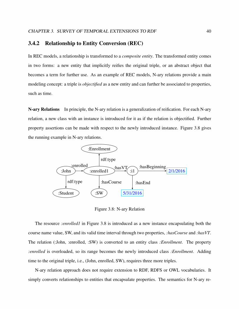
CHAPTER 3. SURVEY OF TEMPORAL EXTENSIONS TO RDF 40
3.4.2 Relationship to Entity Conversion (REC)
In REC models, a relationship is transformed to a composite entity. The transformed entity comes
in two forms: a new entity that implicitly reifies the original triple, or an abstract object that
becomes a term for further use. As an example of REC models, N-ary relations provide a main
modeling concept: a triple is objectified as a new entity and can further be associated to properties,
such as time.
N-ary Relations In principle, the N-ary relation is a generalization of reification. For each N-ary
relation, a new class with an instance is introduced for it as if the relation is objectified. Further
property assertions can be made with respect to the newly introduced instance. Figure 3.8 gives
the running example in N-ary relations.
:enrolled1
:Enrollment
:i1 2/1/2016
5/31/2016
:John
:Student :SW
rdf:type
rdf:type
:hasVT:enrolled
:hasCourse
:hasBeginning
:hasEnd
Figure 3.8: N-ary Relation
The resource :enrolled1 in Figure 3.8 is introduced as a new instance encapsulating both the
course name value, SW, and its valid time interval through two properties, :hasCourse and :hasVT.
The relation (:John, :enrolled, :SW) is converted to an entity class :Enrollment. The property
:enrolled is overloaded, so its range becomes the newly introduced class :Enrollment. Adding
time to the original triple, i.e., (John, enrolled, SW), requires three more triples.
N-ary relation approach does not require extension to RDF, RDFS or OWL vocabularies. It
simply converts relationships to entities that encapsulate properties. The semantics for N-ary re-
CHAPTER 3. SURVEY OF TEMPORAL EXTENSIONS TO RDF 41
lation approach is based on RDF and RDFS semantics. In Figure 3.8, the new object :enrolled1
may also be represented by a blank node. A blank node does not have any meaning, but acts like a
wrapper for grouping related objects.
The running example query in SPARQL is as follows:
SELECT ?ti ?tf
WHERE {
:John :enrolled ?e.
?e rdf:type :Enrollment.
?e :hasCourse :SW.
?e :hasVT ?i.
?i :hasBeginning ?ti.
?i :hasFinish ?tf.
}
While N-ary relation approach can be applied to OWL, it would incur overheads. For instance,
multiple inverse properties are needed for a N-ary relation. Moreover, the use of cardinality re-
strictions becomes limiting on some roles that depend on the class of some other roles [53].
FrameBase FrameBase [60] integrates FrameNet [25] and WordNet [43] for constructing an
extensible RDFS schema. FrameNet originated from Frame Semantics [25]. Frame Semantics as-
sumes that people understand the meaning of words by evoking semantic frames, and relate words
to meanings. FrameNet is a large lexical database that contains semantic frames for describing
meanings of natural language words. It also provides example sentences annotated with frames
and frame elements to demonstrate the use of words in the frame. Each distinct semantic frame
contains lexical units and frame elements. Lexical units are the keywords used to evoke the frame,
while frame elements are the roles that describe properties of the frame.

CHAPTER 3. SURVEY OF TEMPORAL EXTENSIONS TO RDF 42
WordNet [43] is another well known lexical database for English that provides meanings of
words. Each type of words , such as nouns, verbs, adjectives etc. is organized to form a synset,
or a synonym set. Each set represents a lexical concept [43]. WordNet contains about 117,000
synsets, and each may be linked to others. The major relation is hyperonymy,or is A relation, and
meronymy, or part-whole. These relations, among other components, form a lexical network of
words and concepts.
The main representation model used in FrameBase is similar to the model of N-ary relations
discussed above and in Figure 3.8. A primary entity is created to form a semantic frame for
the N-ary relation. The frame’s properties can be asserted in a sense of semantic role [28, 53]. A
mapping between FrameNet and WordNet is created to form the basis lexical units and relations for
FrameBase’s schema.The mapping is further transformed by the schema induction and automatic
reification-dereification mechanism to yield a light weight yet broad covering frames [60].
Valid-Time Temporal Model O’Connor et al. propose a valid-time temporal model and a
SWRL-based [40] query mechanism for manipulating temporal knowledge in OWL ontologies
[55]. The model introduces a new class, temporalFact, and uses N-ary relations. The running ex-
ample is represented in Figure 3.9. The graph in Figure 3.9 is similar to N-ary relations in Figure
3.8. However, there are differences on the class hierarchy. In the valid-time temporal model, any
existing OWL class can have temporal aspects as long as it subclasses temporal:Fact, which is
the super class of all temporal facts. This avoids significant ontology rewriting in converting an
ontology to a temporal version.
The temporal expressivity of this model is further enhanced by using SWRL [40] to construct
temporal rules. A set of temporal operators that includes Allen’s operators [4] is implemented as
library-like built-ins for SWRL rules. With the temporal ontology and temporal built-in operators,
complex temporal rules can be constructed.
Querying the temporal ontology is done by SQWRL [54]. All SWRL built-ins [40] are included

CHAPTER 3. SURVEY OF TEMPORAL EXTENSIONS TO RDF 43
:enrolled1
:Enrollmenttemporal:Fact
:i1 2/1/2016
5/31/2016
:John
:Student :SW
rdf:type
rdf:type
rdfs:subClassOf
:hasVTime
:enrolled
:hasCourse
:hasBeginning
:hasEnd
Figure 3.9: Valid-Time OWL
for SQWRL, so complex temporal queries can be formed. These include queries that require
complex closure, negation, or complex aggregation and grouping. The running example query
is adapted to show temporal operator usefulness in this model. The following SQWRL query
retrieves all resources who took the course :SW before 2016. The symbol ∧ denotes logical and.
Student(?s) ∧ :enrolled(?s, ?e) ∧
:hasCourse(?e, :sw) ∧
temporal:hasValidTime(?e, ?vt) ∧
temporal.before(?vt, "2016")
--> sqwrl:SELECT(?s)
The above query can be transformed to a standard but lengthy SPARQL query. However, there
are very limited temporal operator supports in SPARQL. If done so, the temporal order, such
as temporal:before, may need to be fulfilled by using literal value comparisons. This model is
designed to be implemented at the users’ level. There is no formal extension to RDF, RDFS or
OWL model and vocabularies. However, the additional semantics for Allen’s temporal operator
[4] and the built-in SWRL rules need to be added.

CHAPTER 3. SURVEY OF TEMPORAL EXTENSIONS TO RDF 44
3.4.3 Named Graphs
The term Named graph was first introduced in [18]. Named Graphs extend RDF model to provide
a mechanism for identifying grouped RDF triples. A named graph, denoted by (u1, G1) where
G1 is a standard RDF graph that is named by an IRI ui [18]. W3C has adopted Named Graphs
model in SPARQL query language [58, 32]. With the Named Graph model, the running example
is represented in Figure 3.10.
:john
:sw
:enrolled
:graph1
:hasVT:i1
2/1/2016 5/31/2016
:hasBeginning :hasEnd
Figure 3.10: Named Graph
In Figure 3.10, :graph1 indicates a graph for which additional properties can be asserted. W3C
adopted a line-based N-Quads as concrete syntax for RDF 1.1 Datasets [17]. The format is a quad:
<subject, predicate, object, GraphName>. For querying Named Graphs, TriQL[14], RDFQ [64]
and SPARQL are available. The running example query can be written in SPARQL as follows:
SELECT ?ti ?tf
FROM :graph1
WHERE {:graph1 :hasVT ?i.
?i1 :hasBeginning ?ti.
?i1 :hasEnd ?tf.
:John :enrolled :SW.}

CHAPTER 3. SURVEY OF TEMPORAL EXTENSIONS TO RDF 45
Named Graphs model is a general purpose triple grouping. In the above query, it is assumed that all
triples share the same temporal extent are grouped in the same graph. The FROM clause indicates
the source graph. In an extreme case that each triple requires a different time reference, a significant
amount of named graphs is needed. When triples may need multiple metadata annotation, using
Named Graphs model becomes complex.
τSPARQL Temporal Queries Tappolet et al. propose a temporal RDF query approach τSPARQL
[67]. τSPARQL is defined as a shorthand format for querying such a temporal ontology. In this
model, OWL-Time ontology [37] is used as the time domain which defines time instants and inter-
vals. The target temporal RDF model is designed using Named Graphs. Each graph is identified
by exactly one time interval. Triples with the same temporal extent are grouped to the same graph.
In other words, the name of a graph is the time interval. The grouping also introduces complexity
to the model in that the indexing structure would have a significant impact on query retrieval time.
τSPARQL is based on SPARQL, and recognizes a quadruple form, such as ([ti, tf], s, p, o), as
the main query pattern. The interval [ti, tf] is to be checked against names of graphs. The triple s,
p, o are handled as a SPARQL query pattern. As a result, a τSPARQL query can be mapped to a
standard SPARQL 1.1 one. The running example query can be written in τSPARQL as follows:
SELECT ?ti ?tf
WHERE {
[?ti, ?tf] :John :enrolled :SW.
}
Assuming that the working example is represented as in Figure 3.10, mapping the above query to
standard SPARQL results the following:
SELECT ?ti ?tf
WHERE {

CHAPTER 3. SURVEY OF TEMPORAL EXTENSIONS TO RDF 46
GRAPH :graph1 {:John :enrolled :SW.}
:graph1 :hasBeginning ?ti.
:graph1 :hasEnd ?tf.
}
RDF+ RDF+ model [62] uses named graphs and triple-level identifiers. Named graphs are used
in place of RDF reification. Triple identifiers allow explicit annotation of meta knowledge. RDF+
model has two type of statements: literal and meta knowledge statement. A RDF+ literal statement
is a quintuple form (g, s, p, o, θ) where g is the graph’s IRI, s,p,o are standard RDF triple compo-
nents, and θ is a statement identifier. Based on the triple identifier in the RDF+ literal statement,
the RDF+ meta knowledge statement can be formed as (θ, π, ω). θ is the literal statement identi-
fier, π is the meta knowledge property and ω is the range value of π. The set K of RDF+ literal
statements and the set M of RDF+ meta knowledge statements constitute a RDF+ theory, (K,M)
[62].
Bidirectional mappings between RDF and RDF+ are also defined in [62]. Our running example
is mapped to the RDF+ model and results the following RDF+ literal statements and meta knowl-
edge statement. Please note that we also adapt the N-triple-like syntax for representing a quintuple
in the example. In addition, time intervals are assumed available although the original work uses
time instants.
# K <--RDF+ literal statements
<:graph1> <:John> <:enrolled> <:SW> <:stmtID1>.
<:graph2> <:graph1> <:timestamp>
<[2/1/2016, 5/31/2016)> <:stmtID2>.
# M<--RDF+ meta knowledge statement
<:graph3> <:stmtID1> <:timestamp>

CHAPTER 3. SURVEY OF TEMPORAL EXTENSIONS TO RDF 47
"[2/1/2016, 5/31/2016)".
In the above mapping, :graph1 and stmtID1 both identify the original triple. :graph2 and
:stmtID2 refer to the meta knowledge for :graph1. The statement in :graph2 is further stored
as the associated meta knowledge in order to be compatible with standard RDF semantics. The
formal semantics for RDF+ is provided by ’Meta Knowledge Interpretation and Model’ [62] that
combines a standard interpretation Is for statements in K, and a Π- interpretation for meta knowl-
edge statements in M. An extension to SPARQL is also proposed. The running example query can
be written as follows:
SELECT ?x
WITH META :graph3
FROM NAMED :graph1
FROM NAMED :graph2
WHERE { GRAPH ?g { ?x :enrolled :SW }
The above extended SPARQL utilizes additional constructs: (1) an optional WITH META clause
specifying the graphs which contains the associated meta knowledge, and (2) the FROM NAMED
clause that specifies the target graph for quadruple pattern matching [62]. The query evaluation
system binds the variable ?x to the matched values based on the specified quadruple pattern. It
further outputs values for all meta knowledge associated with the pattern, such as the following:
?x timestamp
---------------------------------
:John [2/1/2016, 5/31/2016)

CHAPTER 3. SURVEY OF TEMPORAL EXTENSIONS TO RDF 48
3.5 Discussion
We have constructed a taxonomy depicted in Figure 3.11 for classifying the proposed temporal
extensions to RDF and OWL. Table 3.2 is a concise summary of various characteristics. For
summarizing and comparing them, we use the following characteristics: (1) RDF, RDFS or OWL
extension of these proposals, (2) additional objects required, (3) number of triples needed, (4)
formal semantics specified or not, (5) Time Domain, (6) Instant or Interval used, and (7) query
language. For completeness, our proposed Valid Time RDF, or VTRDF, is also included in Table
3.2 and the taxonomy in Figure 3.11 for comparison. VTRDF will be introduced in Chapter 4.
Taxonomy The temporal models for the Semantic Web surveyed in this paper use either explicit
or implicit reification. In explicit reification, RDF reification vocabulary or its equivalent is used,
whereas in implicit reification, some form of identification for a triple is introduced.
Temporal RDF [30, 19] and its variants [41, 59] are based on explicit RDF reification. RDF?
introduces nested triples and needs an extension to RDF/S specifications. However, nested triples
in a RDF? graph can be unnested to an explicitly reified RDF graph. Yago2 [38] reifies each
fact and assigns an idenfier to it to form a quintuple. In contrast, all the other temporal models
handle reification implicitly by using different forms of transformation on a triple, relationship
or graph. Such a transformation does not rely on RDF/S reification vocabularies. The type of
transformation differentiates these RDF models: (1)Instantiating-Identifying Concept/Relationship
, (2) Relationship Entity Conversion and (3) Named Graphs.
There are two temporal models in Instantiating-Identifying Concept/Relationship models. 4D
Fluents [73, 6, 7] introduces temporal part for an entity changing over time. Each temporal part
corresponds to a distinguishable timestamp. A fluent property associates two temporal parts. On
the other hand, Singleton Property [52] ensures every relationship to be universally unique. As a
result, an ordinary relationship, such as enrolled, becomes a relationship type. Each of its instances,
such as enrolled#1 in Figure 3.4, is used for an unique property assertion.

CHAPTER 3. SURVEY OF TEMPORAL EXTENSIONS TO RDF 49
N-ary relations, FrameBase and OWL Temporal Model are examples of Relationship Entity
Conversion models. N-ary relations [53] convert each relationship to an entity. FrameBase forms
a semantic frame for each N-ary relation. Frame properties are asserted as semantic roles [28, 53].
OWL Temporal Model [55] is also based on N-ary relations. Lastly, Named Graphs are in RDF
and RDFS specifications. A set of RDF/S triples can be identified with an IRI, that is, the graph
name. Thus, graph level identification becomes available. As a result, additional properties for the
graph can be associated through the graph’s IRI.
RDF, RDFS, OWL Extension and Compliance The majority of models extend RDF/S to gain
temporal expressiveness. For instance, Temporal RDF [30, 19] and its variants [41, 59] introduce
a set of temporal vocabularies to use explicit reification. The model provides a coverage of for-
mal semantics of temporal graphs, query language prototype and complexity analysis. Similarly,
4D Fluents [73, 6, 7], N-ary relations [53] and Named Graphs [18] can all be implemented by
RDF, RDFS and OWL vocabularies. These models benefit from available ontology tools, such as
reasoners.
On the other hand, there are models that require formal extensions to RDF and RDFS specifi-
cations. For instance, Singleton Property [52] introduces rdf:singletonPropertyOf for instantiating
a Singleton Property from its generic property type. Every Singleton Property is made universally
unique. RDF? adopts nested triples to transform a triple to an entity. Nested triples informally
allow triple level identification that is not available in RDF/S or OWL. As a result, RDF? requires
syntactic and semantic extensions to RDF/S and OWL specifications. Similarly, Annotated RDFS
[79] and RDF+ [62] require extensions to both RDF/S syntax and semantics. tOWL [49] extends
OWL-DL to cover concrete domain for representing both time instants and intervals. Furthermore,
it also incorporates Allen’s temporal relations [4] to increase the model’s temporal expressivity.
CHAPTER 3. SURVEY OF TEMPORAL EXTENSIONS TO RDF 50
Additional Objects and Triples When additional objects are required for a temporal model,
they may cause quicker storage depletion or make writing standard queries more complex. The
proliferation of objects is common in reification-based modeling approaches. In Temporal RDF
model [30, 19], eight triples: four for reification and four for temporal assertions, are required
to associate a time interval to an ordinary triple. 4D Fluents [73, 6, 7] use seven triples to cover
temporal parts of an entity. Singleton Property [52] requires fewer triples (five triples). Named-
Graphs [18] require only five temporal assertions, two triples for time instants, three for intervals.
Since RDF+ has a form of quintuple [62] that can be mapped to standard RDF triples via explicit
RDF reification, it requires at least eight triples.
Semantics Typically, a temporal model extending RDF/S or OWL requires additional semantics,
so temporal entailment can be defined. For instance, Temporal RDF [30, 19] specifies a temporal
entailment semantics by using RDF and RDFS graphs. Additionally, this semantics extended
to Enhanced Temporal RDF [41] and tRDF for Indeterminate Triples [59] with added temporal
entailment scenarios, i.e., anonymous timestamp and indeterminate triples respectively.
In contrast, formal extensions to RDF/S or OWL semantics are introduced by extended vocab-
ularies in other models. For instance, Annotated RDF [79] extends RDFS semantics by defining
an algebraic structure for annotation domain, and also provides a deductive system. Singleton
Property [52] requires RDF/S semantics extension to cover its SingletonPropertyOf interpretation.
tOWL [49] requires a semantic extension for the translations between rational numbers, Q, and
XML datetime data types. τSPARQL [67] relies on Named Graphs where the identifier of a graph
is a timestamp instead of an IRI. RDF+ [62] introduces additional semantics for its RDF+ literal
and meta knowledge statement.
Time Domain OWL-Time ontology includes class TemporalEntity [37] which is made-up of
Instants and Intervals. Some of the temporal models use OWL-Time as their time domain. 4D

CHAPTER 3. SURVEY OF TEMPORAL EXTENSIONS TO RDF 51
fluents [73], extended 4D fluents [6, 7] and τSPARQL [67] all employ OWL-Time. The rest of the
models do not use OWL-Time. They typically define a time domain or a time ontology of their
own. For instance, the time domain in Temporal RDF [30, 19] is defined based on natural numbers.
tOWL [49] uses the set of rational numbers, and provides a mapping to actual XML datetime type.
Nevertheless, there are models that do not explicitly adopt a time domain specification. Instead,
the time definition is left to applications.
Querying SPARQL [32, 58] and SQWRL [54] or their extended forms are are used in querying
temporal RDF data. SQWRL is for querying an OWL-based ontology. Temporal RDF [30, 19]
provide a query language sketch in rule-like form. An equivalent SPARQL query can be written
directly, as it is based on RDF reification. Extensions to SPARQL syntax and semantics are needed
for Singleton Property [52], RDF? [33], enhanced Temporal RDF [41, 59], RDF+ [62], τSPARQL
[67], annotated RDF [79] and Extended 4D Fluents [6]. In general, such extension needs to accom-
modate additional patterns of syntax and query specifications. For instance, SPARQL? requires
additional notation for nested triple while RDF+ adds With Meta and From Named constructs for
querying its meta knowledge statements. A dedicated query language TOQL [5] is proposed for
Extended 4D Fluents [6]. AnQL [44] is the query language tailored for Annotated RDFS [79].
SPARQL 1.1 directly supports Named Graphs, so there is no need for a new query language for
Named Graphs [18].

CH
APT
ER
3.SU
RVE
YO
FT
EM
POR
AL
EX
TE
NSIO
NS
TOR
DF
52
Taxonomy of Temporal RDF Models
Explicit Reification
GutierrezTRDF [30, 19]
TRDF variants[41, 59, 79]
RDF?[33]YAGO 2 [38]
Implicit Reification
Instantiating-Identifying
Concept/Relationship (IIR)
4D Fluents[73, 6, 7]
tOWL [49]
SingletonProperty [52]
RelationshipEntity
Conversion (REC)
VT-OWL[55]
N-ary [53]FrameBase [60]
Named Graphs [18]
τSPARQL[67]
RDF+[62]
VTRDF
Figure 3.11: Taxonomy of Temporal RDF Models [72]

CH
APT
ER
3.SU
RVE
YO
FT
EM
POR
AL
EX
TE
NSIO
NS
TOR
DF
53Table 3.2: Temporal Model Comparison [72]
Approach RDF/S Add. # of Triples Semantics Time Domain Inst/Interval QueryExt. Object
Temporal RDF, Enh. N Y 8 RDF/S and Temporal Model Def. Both SWRLYAGO2 quadruple Graph closure Prototype
c-Temporal Graph N Y 8 RDF/S, Temporal Graph Model Def. Both AlgorithmtRDF closure for indeterminate
RDF ? Y Y 7 RDF/S Model Def. Interval SPARQL?
Annotated RDF Y Y N/A1 annotated logic and Model Def. Both AlgorithmInference rules
4D Fluents and Ext. N Y 7 OWL OWL-Time Interval SPARQL
tOWL Y Y 8 OWL-DL Concrete Domain Both SPARQL
Singleton Property Y Y 5 RDF/S ext. Instant SPARQL SPARQL
VT-OWL N Y 8 OWL User User SPARQL
N-ary, FrameBase N Y 7 OWL User User SPARQL
Named Graphs N Y 3 RDF/S User User SPARQL
τ SPARQL N Y 3 RDF/S OWL-Time Both τ SPARQL
RDF+ Y Y Quintuple RDF+ Model Def. Both Ext. SPARQL
VTRDF2 Y N 3 VTRDF Model Def. Interval VT-SPARQL
1 The annotated RDF framework does not discuss its model implementation.
2 VTRDF is our proposed Temporal Model and will be introduced in Chapter 4.

Chapter 4
Valid Time RDF
4.1 Modeling Approach
Hayes introduced the four dimensional view (4D view), also known as perdurantist view, into
Computer Science in his seminal work [35]. Perdurantism is a philosophical theory of persistence
and identity [34]. It is closely related to four dimensionalism. In 4D view, an object that persists
through time has distinct temporal parts at every time instant during its existence in time. Each
persisting object is considered a four dimensional spacetime worm that stretches across the space-
time domain. Slicing the spacetime worm at a specific time instant or interval results a temporal
part or time slice which manifests itself as entity-at-a-time.
In contrast, the three dimensional view (3D view), also known as endurantist view, considers
an object wholly present during its existence in time. There are no temporal parts. In the literature
[63], Sider defended four-dimensionalism based on object identity and part-hood. The arguments
mostly concern whether the identity of the same object remains through times.
Consider that an entity John persists through time. Two time instants characterize his existence
in time: birth and death dates. John was born on January 10, 1995 and is still alive. An interval,
[1/10/1995, now], represents his existence time or valid time. The interval [1/10/1995, now] is
54

CHAPTER 4. VALID TIME RDF 55
closed at both ends. Its lower bound is a standard calendar date in the format of month/day/year or
mm/dd/yyyy, and its upper bound, now, is a special time instant for the current time. In comparison,
entities, such as music, paintings, and scientific theories, may exist indefinitely from its inception
[38]. Their existence time typically has an upper boundary denoted by an infinite instant∞. For
instance, the valid time of Moore’s law [74] is [4/19/1965,∞]. In general, every entity naturally
comes with an existence time which can be represented by a timestamp, such as time points or
intervals.
On the other hand, a fact John attended PS101 describes a binary relationship denoted by the
verb attend, between John and PS101. Among many other modeling approaches , the fact can be
represented in a predicate form: attend(John, PS101). This relationship naturally comes with a
factual time interval, such as [9/1/2008, 6/25/2013), that denotes its validity in time. Adding this
additional time parameter to the relationship results a ternary one, such as attendTemporal(John,
PS101, [9/1/2008, 6/25/2013)) where attendTemporal is the 3-ary predicate name. Alternatively,
a second order relationship, or nested relationship, also suits the same modeling case, such as
attendTemporalNested(attend(John, PS101), [9/1/2008, 6/25/2013)) where attendTemporalNested
is a 2-ary predicate name. Nevertheless, neither can be represented directly in RDF which requires
binary relationships fundamentally.
From the above observation, we know that every entity or relationship naturally comes with
a valid timestamp. As a result, a binary relationship actually incurs three timestamps: the valid
time of the relationship and two participating entities. To fully preserve the temporal aspect of the
binary relationship, all three timestamps shall be incorporated into the model. This is a modeling
problem similar to the case of defining N-ary or high order relations in the Semantic Web [53].
With the John’s example mentioned above and the 4D view interpretation, we found that it is
actually that the temporal part of John was associated with the temporal part that corresponded
to the same time period when PS101 had John as an elementary school student. This is due to
that in the 4D view, entities spread through time instead of ranging over time. ‘Entities spreading

CHAPTER 4. VALID TIME RDF 56
through time’means that they only exist for some period of time, whereas ‘entities ranging over
time’reflects that they are wholly present. Although John is the main entity, the identity of John in
[9/1/2008, 6/25/2013) is conceptually distinguishable from that of John in [9/1/2013, 6/25/2015).
In this thesis, we adopt a modeling approach that employs ideas from the 4D view and orig-
inated from the study in [66], and propose the Valid Time RDF, or VTRDF in short. VTRDF is
based on temporal resource and temporal relationship or temporal fact. A temporal resource is a
RDF-compliance resource equipped with a timestamp to denote its existence in time. Each tem-
poral resource is a coalesce of all its temporal parts. In other words, a temporal resource is wholly
present during its existence in time. Temporal parts are derived by slicing or projecting a temporal
resource on to the time dimension. A temporal relationship is formed between either temporal
parts or temporal resources provided that the participating or parts or resources coexist in time. A
temporal relationship is a factual assertion that relates qualified temporal resources.
We base the VTRDF model on the standard RDF model and its model semantics. A standard
RDF triple (s, p, o) contains elements that are all resources: s, p, o ∈ R, and R is an infinite set
of resources. We introduce VTR, an infinite set of valid time resources, as the building block for
VTRDF triples and VTRDF graphs. A valid time resource is a resource with its existence time
or valid time. In VTRDF, we consider a valid time resource as a collection of all its temporal
parts. Assertions can be made with respect to both the collection and any individual temporal part.
A temporal resource is a master resource, whereas all its temporal parts are member resources.
Projections from the master resource to its temporal parts are possible via projection functions.
The temporal aspects of the resources can use valid time, transaction time, or bitemporal. In this
research, we focus on the valid time. Hence, we would use valid time resources and temporal
resources interchangeably as appropriate.

CHAPTER 4. VALID TIME RDF 57
4.2 Notations, Namespace, and Time Domain
In the remainder of this chapter, we will define VTRDF and present examples. As introduced
in section 2.4, we still use the graph-based representation for illustrating VTRDF examples. For
instance, in Figure 4.1, an oval denotes a temporal resource as a subject or object, and a literal as an
object. A directed link represents a predicate. When a literal value is used, it is double quoted and
annotated with a data type or a language tag. When necessary, we also use the line-based Turtle
syntax [9] to serialize VTRDF triples and graphs.
resource 1 resource 2 or literalpredicate 1
Figure 4.1: Graph Notation for VTRDF
The prefix rdf:, rdfs:, and xsd: have been defined in section 2.4, and their uses remain in
VTRDF. Besides, we introduce new namespace, summarize as follows:
@PREFIX vtrdf: <http://example.org/vtrdf-syntax#>
@PREFIX vtrdfs: <http://example.org/vtrdf-schema#>
@PREFIX xsd: <http://www.w3.org/2001/XMLSchema#>
@PREFIX : <http://example.org/temporal-SW#>
The customized prefix vtrdf: and vtrdfs: refer to the namespace of VTRDF vocabulary and
VTRDF Schema vocabulary respectively. Well use a base ontology for the running example, ex-
plained in the next section, to illustrate syntax and semantics of the VTRDF model. It assumes the
Namespace http://example.org/temporal-SW, and we use : (colon) as its prefix.
While the symbol # is used to denote an additional part of the primary resource in the standard
RDF model, VTRDF requires a second fragment identifier to accommodate the valid time dimen-
sion. The symbol • is used as a delimiter that separates the first fragment identifier from the valid

CHAPTER 4. VALID TIME RDF 58
time. For instance, the IRI http://example.org/temporal-SW#John•[1/10/1995–now] denotes the
complete valid time resource which embeds a valid time interval.
For the time domain, we follow the definitions given in section 3.2. Main terms for the time
domain are summarized as follows:
• T is the set of time points with a linear order less-than (<). For simplicity, we use the
standard U.S. calendar dates as the unit of time points in the format of month/day/year, such
as 1/10/1995.
• TI is the set of time intervals defined over T , as follows:
TI = {[l, u)|l ∈ T ∧ u ∈ T ∧ l < u} (4.2.1)
• 0 is the lower bound of the time axis whose interpretation is open for user’s need of data
modeling.
• now is a special constant that represents the current time. Its value will change as time
advances.
• ∞ is a constant that represents the upper bound of the time axis.
• [0,∞] is a special interval used to represent the maximal interval.
4.3 Running Example
We follow the same relation given in Table 2.3 which considers a 4-ary relation: Person(John, SW,
NYC, [2/1/2016, 5/31/2016]). Recall that it represents an individual person whose name is John.
For simplicity, we also use the term John as an identifier. John enrolled in the Semantic Web course
(SW), lived in New York City (NYC), and had a valid time [2/1/2016, 5/31/2016). To represent the
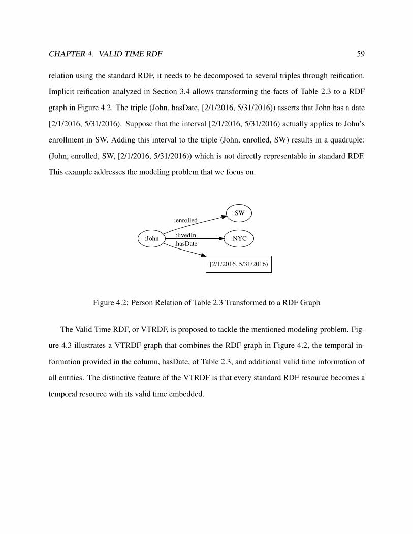
CHAPTER 4. VALID TIME RDF 59
relation using the standard RDF, it needs to be decomposed to several triples through reification.
Implicit reification analyzed in Section 3.4 allows transforming the facts of Table 2.3 to a RDF
graph in Figure 4.2. The triple (John, hasDate, [2/1/2016, 5/31/2016)) asserts that John has a date
[2/1/2016, 5/31/2016). Suppose that the interval [2/1/2016, 5/31/2016) actually applies to John’s
enrollment in SW. Adding this interval to the triple (John, enrolled, SW) results in a quadruple:
(John, enrolled, SW, [2/1/2016, 5/31/2016)) which is not directly representable in standard RDF.
This example addresses the modeling problem that we focus on.
:John
:SW:enrolled
:NYC:livedIn
[2/1/2016, 5/31/2016)
:hasDate
Figure 4.2: Person Relation of Table 2.3 Transformed to a RDF Graph
The Valid Time RDF, or VTRDF, is proposed to tackle the mentioned modeling problem. Fig-
ure 4.3 illustrates a VTRDF graph that combines the RDF graph in Figure 4.2, the temporal in-
formation provided in the column, hasDate, of Table 2.3, and additional valid time information of
all entities. The distinctive feature of the VTRDF is that every standard RDF resource becomes a
temporal resource with its valid time embedded.
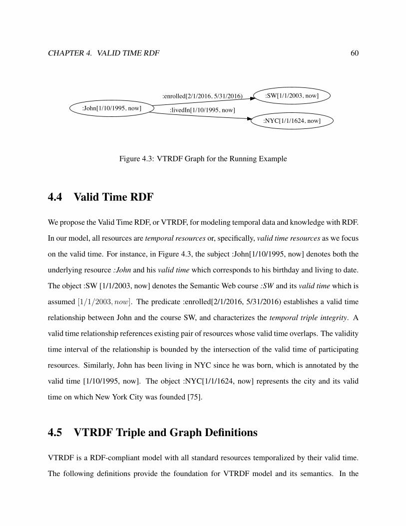
CHAPTER 4. VALID TIME RDF 60
:John[1/10/1995, now]
:SW[1/1/2003, now]:enrolled[2/1/2016, 5/31/2016)
:NYC[1/1/1624, now]:livedIn[1/10/1995, now]
Figure 4.3: VTRDF Graph for the Running Example
4.4 Valid Time RDF
We propose the Valid Time RDF, or VTRDF, for modeling temporal data and knowledge with RDF.
In our model, all resources are temporal resources or, specifically, valid time resources as we focus
on the valid time. For instance, in Figure 4.3, the subject :John[1/10/1995, now] denotes both the
underlying resource :John and his valid time which corresponds to his birthday and living to date.
The object :SW [1/1/2003, now] denotes the Semantic Web course :SW and its valid time which is
assumed [1/1/2003, now]. The predicate :enrolled[2/1/2016, 5/31/2016) establishes a valid time
relationship between John and the course SW, and characterizes the temporal triple integrity. A
valid time relationship references existing pair of resources whose valid time overlaps. The validity
time interval of the relationship is bounded by the intersection of the valid time of participating
resources. Similarly, John has been living in NYC since he was born, which is annotated by the
valid time [1/10/1995, now]. The object :NYC[1/1/1624, now] represents the city and its valid
time on which New York City was founded [75].
4.5 VTRDF Triple and Graph Definitions
VTRDF is a RDF-compliant model with all standard resources temporalized by their valid time.
The following definitions provide the foundation for VTRDF model and its semantics. In the

CHAPTER 4. VALID TIME RDF 61
remainder of this chapter, we use VTRDF graph instances in the examples.
Definition 4.5.1. Valid Time Resource
LetR be an infinite set of standard RDF resources, TI be the set of intervals and V TR = R×TI
be their Cartesian product. A valid time resource rt ∈ V TR is a resource with a timestamp that
denotes its validity in time. A valid time resource is formed by the concatenation of a standard
resource r ∈ R and i ∈ TI to integrate both its resource and valid time parts, i.e. r•i where • is a
delimiter. The valid time resource is a special case in considering other attributes of time, such as
transaction time or bitemporal. In the case of transaction time, a transaction time resource is the
concatenation of a standard resource and its transaction time that denotes when it is recorded or
created in the database.
Definition 4.5.2. Valid Time Internationalized Resource Identifier
A valid time Internationalized Resource Identifier (IRI) is used to denote a valid time resource
uniquely. It consists of two parts. The first denotes a resource, and the second denotes its valid
time. The resource part employs the IRI specification used in standard RDF, which may contain a
fragment identifier as specified in section 4.2. The valid time is added as the second fragment iden-
tifier by a delimiter •, while the first fragment identifier starts with the delimiter #. The following
is a valid time IRI resource that denotes a resource John whose valid time is [1/10/1995, now]:
http://example.org/temporal-SW#John•[01-10-1995–now]
In the remainder of this thesis, we sometimes abuse this notation and do not include the second
delimiter, in representing temporal resources.
Definition 4.5.3. Valid Time Literal
Let L be an infinite set of standard literals, [0,∞] the maximal interval, and V TL = L× [0,∞]
be the Cartesian product. A valid time literal lt ∈ V TL represents a literal that is always valid in
time. That is, all literals assume a default maximal interval [0,∞] unless otherwise specified.

CHAPTER 4. VALID TIME RDF 62
Definition 4.5.4. Valid Time Data Type
Let D be an infinite set of standard data types, [0,∞] the maximal interval, and V TD =
D × [0,∞] be the Cartesian product. A valid time data type dt ∈ V TD is a data type recognized
in the standard RDF with a default maximal interval [0,∞]. In other words, all valid time data
types are always valid in time. Valid time data types are used to annotate valid time literals.
For instance, ”1”∧∧ xsd:integer[0,∞] denotes an integer 1 by the XML Schema integer type. A
special data type vtrdf:langString[0,∞] can also be used to denote a language-tagged string value.
For instance, ”Neuva York City”@sp[0,∞] is a valid time literal ”New York City” in a Spanish
language tag.
Definition 4.5.5. Lexical-to-Value Mapping Function V TL2V
V TL2V is a partial mapping from the lexical space of valid time literals to the value space V .
A valid time literal lt with a valid time data type dt denote the mapped value obtained from the
value space. That is, V TL2V (lt, dt) = v where v ∈ V .
Definition 4.5.6. Valid Time Property
Let P be the set of any properties, including those defined in RDF and RDFS vocabularies
[16], TI be the set of intervals, and V TP = P ×TI be the Cartesian product of them. A valid time
property pt ∈ V TP is any property that is valid during a specified interval i ∈ TI .
Definition 4.5.7. Valid Time Blank Node
Let B be an infinite set of blank nodes, TI be the set of intervals, and V TB = B × TI be the
Cartesian product. A valid time blank node bt ∈ V TB denotes the existence of a resource whose
valid time may or may not be known. For simplicity, every valid time blank node in the VTRDF
model assumes a default maximal valid interval [0,∞] unless otherwise specified. A valid time
blank node is usually identified by a local identifier.
Definition 4.5.8. Valid Time Resource Projection Function

CHAPTER 4. VALID TIME RDF 63
A valid time resource projection function, fk : V TR→ [R|TI |T |V TR], k = {res, vt, vts, vte, i},
takes a valid time resource rt ∈ V TR and projects to either the resource dimension (subscripted
res), the valid time dimension (subscripted vt) which is further categorized to vts and vte for the
beginning and end of the interval, or a slice of the resource rt at the interval i (parameterized
(rt, i)). Given a valid time resource rt = r[l, u) ∈ V TR, the projection function characterizes the
following cases.
• Resource Projection
Πresrt = r (4.5.1)
• Valid Time Projection
Πvtrt = [l, u) (4.5.2)
Πvtsrt = l (4.5.3)
Πvtert = u (4.5.4)
• Resource Slice Projection given an interval i
Π(i, rt) = rt1 where Πresrt1 = Πresr
t and Πvtr1 = i ∩ Πvtrt (4.5.5)
In addition, we overload the projection function to accommodate operations for valid time blank
nodes. As a blank node is not given a valid time IRI, its resource part is undefined. Its resource
projection therefore results a locally-scoped identifier which has been assigned. In other words,

CHAPTER 4. VALID TIME RDF 64
given a valid time blank node bt, we have:
Πresbt = locally-scopped identifier (4.5.6)
Πvtbt = [l, u) (4.5.7)
In the case of the slice projection function, we also call the resulting resource a slice of the
original valid time resource. Furthermore, a shortcut dot notation (.) is also used in place of the
algebraic forms, such as rt.res = Πresrt.
As an example, given a valid time resource rt= :John[1/10/1995, now] and i = [2/1/2016, 5/31/2016),
we have the following:
Πresrt = :John (4.5.8)
Πvtrt = [1/10/1995, now] (4.5.9)
Πvtsrt = 1/10/1995 (4.5.10)
Πvtert = now (4.5.11)
Π(rt, i) = :John[2/1/2016, 5/31/2016) (4.5.12)
Definition 4.5.9. Valid Time RDF Triple
Let st, pt, ot be VTRDF resources defined as follows. They represent the subject, the predicate,
and the object respectively.

CHAPTER 4. VALID TIME RDF 65
• st ∈ V TR ∪ V TB
• pt ∈ V TP
• ot ∈ V TR ∪ V TB ∪ V TL
A Valid Time RDF triple (st, pt, ot) satisfies the temporal constraint, called Temporal Triple In-
tegrity , as follows:
Πvt(pt) ⊆ Πvt(s
t) ∩ Πvt(ot) where Πvt(s
t) ∩ Πvt(ot) 6= ∅. (4.5.13)
The integrity constraint enforces that the valid time of the property or predicate pt ∈ V TP is
bounded by the interval that is formed by the common valid time of st and ot. In other words, the
temporal triple integrity requires that a valid time relationship can only be established between two
existing resources with non-disjoint valid time.
Definition 4.5.10. Predicate Defining Time (PDT) and Resource Modeling Time (RMT)
Any valid time resource rt ∈ V TR takes one of the Predicate Defining Time (PDT) or Re-
source Modeling Time (PMT) based on its use in VTRDF triples.
• Predicate Defining Time (PDT):
rt takes PDT when it is used in a VTRDF triple as a predicate to define the time of a re-
lationship. In this case, PDT corresponds to the interval during which the relationship is
valid.
• Resource Modeling Time (RMT):
rt takes RMT when it is used in a VTRDF triple as a subject or an object that eventually
involves in a relationship. RMT is the time that we want to store about the facts into the
database. Given rt for each subject or object, it always has a unique RMT as its valid time.

CHAPTER 4. VALID TIME RDF 66
Definition 4.5.11. VTRDF Graph
A VTRDF graph Gt is a set of VTRDF triples defined as follows :
Gt = {(st, pt, ot)|st ∈ (V TR ∪ V TB) ∧ pt ∈ V TP ∧ ot ∈ (V TR ∪ V TL ∪ V TB)∧
(pt.vt ⊆ st.vt ∩ ot.vt)∧
(st.vt ∩ ot.vt 6= ∅)∧
¬∃((xt, yt, zt)((st.res = xt.res ∧ pt.res = yt.res ∧ ot.res = zt.res∧
(st.vt ∩ xt.vt 6= ∅ ∨ st.vte = xt.vts)∧
(pt.vt ∩ yt.vt 6= ∅ ∨ pt.vte = yt.vts)∧
(ot.vt ∩ zt.vt 6= ∅ ∨ ot.vte = zt.vts))∨
¬∃(xt, yt, zt)(st.res = zt.res ∧ st.vt ∩ zt.vt 6= ∅)∨
¬∃(xt, yt, zt)(ot.res = xt.res ∧ ot.vt ∩ xt.vt 6= ∅)}
(4.5.14)
Definition 4.5.12. Valid Timeslice Operator
Given a VTRDF graph Gt and an interval i = [l, u), the valid time slice operator, TS, returns a
temporal subgraph of Gt at i, defined as follows:
TS(Gt1, i) : Gt
1 → Gt2 (4.5.15)
Gt2 = {(st1, pt1, ot1)|(st, pt, ot) ∈ Gt
1 ∧ st1.res = st.res ∧ pt1.res = pt.res ∧ ot1.res = ot.res∧
i1 = (i ∩ st.vt ∩ pt.vt ∩ ot.vt) ∧ i1 6= ∅ ∧ st1.vt = i1 ∧ pt1.vt = i1 ∧ ot1.vt = i1}
(4.5.16)
TS takes a VTRDF graph Gt1 and an interval i as arguments. The resource slice projection

CHAPTER 4. VALID TIME RDF 67
function of the Definition 4.5.8 is then applied to component resources of triples in Gt1. Hence,
this operation creates a new VTRDF graph, Gt2, from Gt
1 provided i overlaps with the valid time
of subjects, predicates, and objects appear in Gt1. Otherwise, TS returns an empty set. Please note
that a legal VTRDF triple satisfies the temporal triple integrity specified Definition 4.5.9. Hence,
the condition (i ∩ st.vt ∩ pt.vt ∩ ot.vt) in Expression 4.5.16 can be reduced to (i ∩ pt.vt).
Suppose that Gt1 denotes the running example shown in Figure 4.3, Figure 4.4 shows a VTRDF
graphGt2 derived from the graphGt
1 by applying theTS operation toGt1 at [2/1/2016, 5/31/2016).
:John[2/1/2016, 5/31/2016)
:SW[2/1/2016, 5/31/2016):enrolled[2/1/2016, 5/31/2016)
:NYC[2/1/2016, 5/31/2016):livedIn[2/1/2016, 5/31/2016)
Figure 4.4: VTRDF Graph for the Running Example Sliced at the Interval [2/1/2016, 5/31/2016)
Definition 4.5.13. VTRDF Subgraph
A VTRDF graph H t is a subgraph of another VTRDF graph Gt if H t includes some of the
VTRDF triples in Gt. For instance, the VTRDF graph in Figure 4.5 is a subgraph of the graph in
Figure 4.3.
:John[1/10/1995, now] :SW[0, ∞]:enrolled[2/1/2016, 5/31/2016)
Figure 4.5: A VTRDF Subgraph of the Running Example in Figure 4.3
Additionally, a valid timeslice of a VTRDF graph Gt is a temporal subgraph of it. That is, the

CHAPTER 4. VALID TIME RDF 68
graph in Figure 4.4 is a temporal subgraph of the graph in Figure 4.3.
Definition 4.5.14. VTRDF Underlying Triple
Given a VTRDF triple e = (st, pt, ot), its underlying triple u(e) is defined as:
u(e) = (Πresst,Πresp
t,Πresot) (4.5.17)
Definition 4.5.15. VTRDF Underlying Graph
Given a VTRDF graph Gt, its underlying graph u(Gt) is defined as:
u(Gt) = {(u(e)|e ∈ Gt} where e is a VTRDF triple (4.5.18)
u(Gt) becomes a standard RDF graph. Duplicate triples are eliminated. If two or more triples
agree on the subject or object, they are combined to one triple. As an example, the underlying
graph of the VTRDF graph in Figure 4.3 is shown in Figure 4.6.
:John
:SW:enrolled
:NYC
:livedIn
Figure 4.6: A VTRDF Underlying Graph of the Running Example in Figure 4.3
Definition 4.5.16. VTRDF Graph Vocabulary
Given a VTRDF graphGt and the set of valid time resources V TR appear inGt, the vocabulary
voc(Gt) is the set of valid time IRIs that appear in Gt excluding valid time literals.
Definition 4.5.17. Ground VTRDF Graph
A ground VTRDF graph is a VTRDF graph that does not contain any valid time blank nodes.
CHAPTER 4. VALID TIME RDF 69
Definition 4.5.18. VTRDF Mapping Function
A mapping function, M t : (V TR ∪ V TB ∪ V TL) → (V TR ∪ V TB ∪ V TL), maps a valid
time resource, a valid time literal, or a valid time blank node to a valid time resource, a valid time
literal, or another valid time blank node. M t is defined to map elements of one VTRDF graph to
another. Four mapping cases at the resource level are defined for two given VTRDF graphs Gt1 and
Gt2 as follows:
• M t(rt1) = rt2 where rt1 ∈ Gt1, r
t2 ∈ Gt
2, r1.res = r2.res, and r1.vt = r2.vt.
• M t(lt1) = lt2 where lt1 ∈ Gt1, l
t2 ∈ Gt
2, l1.res = l2.res, and l1.vt = l2.vt.
• M t(bt) = rt where bt ∈ Gt1, bt.vt = [0,∞], rt ∈ Gt
2 and rt.vt ⊆ bt.vt.
• M t(bt1) = bt2 where bt1 ∈ Gt1, and bt2 ∈ Gt
2.
In addition, M t can be overloaded to map a VTRDF graph. Given a VTRDF graphGt, M t(Gt)
maps to a set of all (M t(st),M t(pt),M t(ot) where (st, pt, ot) ∈ Gt.
4.6 VTRDF Vocabulary (vtrdfV)
VTRDF is formulated as layers and RDF-compliant. VTRDF triples and graphs are constructed
and manipulated as they are in the standard RDF model. Basic VTRDF triple assertions are at the
base layer which is augmented by VTRDF vocabularies, and further by VTRDF schema vocabu-
laries. VTRDF provides ontological modeling primitives to define terminology vocabularies and
use them for asserting facts while incorporating valid time herein.
Figure 4.7 shows the serialization for the running example of Figure 4.3 in Turtle syntax [9].
As discussed in section 4.4, each component in a VTRDF triple denotes a standard RDF resource
and its valid time altogether. The main advantage of using VTRDF is self-explanatory. We are able
to capture the fact that John, who is identified as a standard RDF resource, was born on 1/10/1995

CHAPTER 4. VALID TIME RDF 70
and now is alive. In addition, NYC and SW both exist permanently since their inception. enroll
and liveIn are both valid time properties that relate two valid time resources and satisfy Temporal
Triple Integrity of Definition 4.5.9. By checking the following two expressions (4.6.1) and (4.6.2),
we assure that the triples in Figure 4.7 are valid VTRDF triples.
PREFIX : http://example.org/temporal-SW#>
:John[1/10/1995,now] :enrolled[2/1/2016,5/31/2016) :SW[1/1/2003, now].
:John[1/10/1995,now] :liveIn[1/10/1995,now] :NYC[1/1/1624, now].
Figure 4.7: Running Example in Turtle Syntax
[2/1/2016, 5/31/2016) ⊆ [1/10/1995, now] ∩ [1/1/2003, now] (4.6.1)
[1/10/1995, now] ⊆ [1/10/1995, now] ∩ [1/1/1624, now] (4.6.2)
A set of vocabularies, called VTRDF vocabulary, or vtrdfV, is defined below. vtrdfV augments
the VTRDF model with more expressive power.
• vtrdf:type[l, u) is a valid time property that has different temporal references depending on
how it is used. The type property holds valid during [l, u) as a predicate defining time given
in section 4.5.10. vtrdf:type[l, u) can also be used in the subject or object position. In this
case, [l, u) corresponds to resource modeling time given in Definition 4.5.10.
• vtrdf:Property[l, u) is the valid time class of all valid time properties with a coalesced valid
time,[l, u), from all of its instances. As the class denotes a generic class in time, we may
assign the maximal interval [0,∞] as its valid time. Otherwise [l, u) is used.
• vtrdf:Statement[l, u) is the valid time class of all VTRDF statements. The class denotes a
generic concept in time, and we may assign the maximal interval [0,∞] as its valid time.
Otherwise [l, u) is used.

CHAPTER 4. VALID TIME RDF 71
• vtrdf:subject[l1, u1), vtrdf:predicate[l2, u2) and vtrdf:object[l3, u3) are valid time properties
used to assert the subject, predicate and the object of a VTRDF statement respectively. They
are intended to be used in the reification.
By using VTRDF vocabularies, additional knowledge about the running example of Figure 4.3
can be expressed. Figure 4.8 shows a graph that contains three fresh facts: John is a student in
[2/1/2016, 5/31/2016), NYC is a city that was founded in 1624, and SW is a course established on
1/1/2003. City and Course are likewise having the valid time that reflects their lifespan.
:John[1/10/1995, now]
:Student[1/1/1970, now]
vtrdf:type[2/1/2016, now]
:SW[1/1/2003,now]
:enrolled[2/1/2016, 5/31/2016)
:NYC[1/1/1624, now]
:livedIn[1/10/1995, now]
:Course[1/1/1970, now]
vtrdf:type[1/1/2003, now]
:City[1/1/1500, now]
vtrdf:type[1/1/1624, now]
Figure 4.8: Running Example with Additional Facts in VTRDF Vocabulary (vtrdfV)
Each valid time triple in Figure 4.8 satisfies the temporal triple integrity in the Definition 4.5.9.
In addition, special temporal constraints could be imposed depending on the modeling needs. For
instance, the graph in Figure 4.9 is a subgraph of Figure 4.8. Suppose a constraint that the property
enrolled is applicable to John only when he is a student has to be imposed. That is, the valid time
of the enrolled property should be the subset of the valid time of the type property for student. In
the VTRDF model, such a constraint can be enforced as a special temporal constraint.
In addition, a set of axioms, shown in Figure 4.10, follows from the above definitions of vtrdfV.
Each axiom satisfies the temporal triple integrity in Definition 4.5.9: [l2, u2) ⊆ [l1, u1) ∩ [l3, u3).

CHAPTER 4. VALID TIME RDF 72
:John[1/10/1995, now]
:Student[1/1/1970, now]
vtrdf:type[2/1/2016, now]
:SW[1/1/2003,now]
:enrolled[2/1/2016, 5/31/2016)
Figure 4.9: A Subgraph of Figure 4.8
PREFIX vtrdf: <http://example.org/vtrdf-syntax#>
vtrdf:type[l1, u1) vtrdf:type[l2, u2) vtrdf:Property[l3, u3).
vtrdf:subject[l1, u1) vtrdf:type[l2, u2) vtrdf:Property[l3, u3).
vtrdf:predicate[l1, u1) vtrdf:type[l2, u2) vtrdf:Property[l3, u3).
vtrdf:object[l1, u1) vtrdf:type[l2, u2) vtrdf:Property[l3, u3).
Figure 4.10: Axioms of VTRDF Vocabulary (vtrdfV)
4.7 VTRDF Schema Vocabulary (vtrdfsV)
VTRDF Schema Vocabulary, or vtrdfsV, augments VTRDF to provide more semantic constructs,
including valid time classes and their properties.
Definition 4.7.1. Valid Time Class
Let C be an infinite set of standard classes, TI be the set of intervals, and V TC = C × TI be
the Cartesian product. A valid time class ct ∈ V TC is a class whose valid time is the union of the
valid time of all its member resources. Practically, a maximal interval [0,∞] is assigned to every
valid time class unless otherwise specified.

CHAPTER 4. VALID TIME RDF 73
Valid time classes in VTRDF schema denote generic concepts, therefore they are all assigned
the maximal interval as their valid time. In addition, valid time properties are used to define
relationships between valid time resources, and they take predicate defining time as their valid
time. vtrdfsV is defined as follows:
• Valid Time Classes:
– vtrdfs:Resource[l, u) is the superclass of all valid time resources.
– vtrdfs:Literal[l, u) is the class of all valid time literals.
– vtrdfs:Class[l, u) is the class of all valid time classes.
• Valid Time Properties:
– vtrdfs:domain[l, u) defines the domain of a valid time property. It can also be used to
define itself.
– vtrdfs:range[l, u) defines the range of a valid time property. It can also be used to define
itself.
– vtrdfs:subClassOf[l, u) defines the valid time class hierarchy.
– vtrdfs:subPropertyOf[l, u) defines the valid time property hierarchy.
A set of axioms in Figure 4.11, written in Turtle syntax [9], follows from the above definitions
of valid time classes and properties. The temporal triple integrity specified in the Definition 4.5.9
applies to all axioms.
By using the valid time classes, class properties, and the set of VTRDFS axioms, inference can
be made. Entailed knowledge can be explicitly added. For instance, the type range axiom in Figure
4.11 allows us to infer that the resources :Student[1/1/1970, now], :Course[1/1/1970, now] and
:City[1/1/1500, now] are all range values of specific type assertions. Therefore they are valid time

CHAPTER 4. VALID TIME RDF 74
PREFIX vtrdf: <http://example.org/vtrdf-syntax#>
PREFIX vtrdfs: <http://example.org/vtrdf-schema#>
vtrdfs:Class[l1, u1) vtrdfs:subClassOf[l2, u2) vtrdfs:Resource[l3, u3).
vtrdfs:Property[l1, u1) vtrdfs:subClassOf[l2, u2) vtrdfs:Resource[l3, u3).
vtrdfs:Literal[l1, u1) vtrdfs:subClassOf[l2, u2) vtrdfs:Resource[l3, u3).
vtrdf:type[l1, u1) vtrdfs:domain[l2, u2) vtrdfs:Resource[l3, u3).
vtrdf:type[l1, u1) vtrdfs:range[l2, u2) vtrdfs:Class[l3, u3).
vtrdfs:domain[l1, u1) vtrdfs:domain[l2, u2) vtrdf:Property[l3, u3).
vtrdfs:domain[l1, u1) vtrdfs:range[l2, u2) vtrdfs:Class[l3, u3).
vtrdfs:range[l1, u1) vtrdfs:domain[l2, u2) vtrdf:Property[l3, u3).
vtrdfs:range[l1, u1) vtrdfs:range[l2, u2) vtrdfs:Class[l3, u3).
vtrdfs:subClassOf[l1, u1) vtrdfs:domain[l2, u2) vtrdfs:Class[l3, u3).
vtrdfs:subClassOf[l1, u1) vtrdfs:range[l2, u2) vtrdfs:Class[l3, u3).
vtrdfs:subPropertyOf[l1, u1) vtrdfs:domain[l2, u2) vtrdf:Property[l3, u3).
vtrdfs:subPropertyOf[l1, u1) vtrdfs:range[l2, u2) vtrdf:Property[l3, u3).
Figure 4.11: Axioms of VTRDF Schema Vocabulary (vtrdfsV)
classes. The inferred triples are shown in Figure 4.12 and we are adding them to the graph of
Figure 4.8. Figure 4.13 shows the updated graph. Please note that the definitions of the inference
and entailment will be discussed in the section 4.8.
:Student[1/1/1970, now] vtrdf:type[1/1/1970, now] vtrdfs:Class[1/1/1970, now].
:Course[1/1/1970, now] vtrdf:type[1/1/1970, now] vtrdfs:Class[1/1/1970, now].
:City[1/1/1500, now] vtrdf:type[1/1/1970, now] vtrdfs:Class[1/1/1970, now].
Figure 4.12: Inferred Triples Based on the Range Axiom in Figure 4.11
Furthermore, properties about :enrolled[2/1/2016, 5/31/2016) and :livedIn[1/10/1995, now]
can be asserted by using vtrdfs:domain[l1, u1) and vtrdfs:range[l2, u2). In this way, they are de-
fined as terminology vocabularies which are used to assert facts. Figure 4.14 shows the complete
knowledge base, written in Turtle syntax [9], of the running example originally illustrated in Figure

CHAPTER 4. VALID TIME RDF 75
4.3.
:John[1/10/1995, now]
:Student[1/1/1970, now]
vtrdf:type[2/1/2016, now]
:SW[1/1/2003, now]
:enrolled[2/1/2016, 5/31/2016)
:NYC[1/1/1624, now]
:livedIn[1/10/1995, now]
vtrdfs:Class[1/1/1500, now]
vtrdf:type[1/1/1970, now] :Course[1/1/1970, now]
vtrdf:type[1/1/2003, now]
:City[1/1/1500, now]
vtrdf:type[1/1/1624, now]
vtrdf:type[1/1/1970, now] vtrdf:type[1/1/1500, now]
Figure 4.13: Running Example with Additional Facts in VTRDF Schema Vocabulary (vtrdfsV)

CHAPTER 4. VALID TIME RDF 76
:enrolled[2/1/2016, 5/31/2016) vtrdfs:domain[2/1/2016, 5/31/2016)
:Student[1/1/1970, now].
:enrolled[2/1/2016, 5/31/2016) vtrdfs:range[2/1/2016, 5/31/2016)
:Course[1/1/1970, now].
:livedIn[1/10/1995, now] vtrdfs:domain[1/10/1995, now] :Student[1/1/1970, now].
:livedIn[1/10/1995, now] vtrdfs:range[1/10/1995, now] :City[1/1/1500, now].
:SW[1/1/2003, now] vtrdf:type[1/1/2003, now] :Course[1/1/1970, now].
:Student[1/1/1970, now] vtrdf:type[1/1/1970, now] vtrdfs:Class[1/1/1500, now].
:Course[1/1/1970, now] vtrdf:type[1/1/1970, now] vtrdfs:Class[1/1/1500, now].
:City[1/1/1500, now] vtrdf:type[1/1/1500, now] vtrdfs:Class[1/1/1500, now].
:John[1/10/1995, now] vtrdf:type[2/1/2016, now] :Student[1/1/1970, now].
:John[1/10/1995, now] :enrolled[2/1/2016, 5/31/2016) :SW[1/1/2003, now].
:John[1/10/1995, now] :livedIn[1/10/1995, now] :NYC[1/1/1624, now].
Figure 4.14: Complete Knowledge Base of the Original Running Example with Additional Factsin Turtle Syntax

CHAPTER 4. VALID TIME RDF 77
4.8 VTRDF Semantics and Entailment
Now the focus turns to the formal semantics of the VTRDF model. The standard RDF 1.1 [36]
employs the model-theoretic semantics which introduces interpretation models and semantic con-
ditions for its layered vocabularies of RDF and RDFS. In VTRDF, we characterize the model se-
mantics in four groups of vocabularies, and define formal semantics accordingly for each group. In
each group, an interpretation model is defined based on interpretation domain and a set of semantic
conditions for its vocabularies. These groups of vocabularies are:
1. Simple Vocabulary (V t)
V t refers to vocabularies without valid time data types Dt, vtrdfV, or vtrdfsV. That is, V t ∩
(vtrdfV ) ∩ (vtrdfsV ) = ∅.
2. Simple Vocabulary with Valid Time Data Types (V t-Dt)
V t-Dt includes the simple vocabulary V t and the Valid Time data type Dt.
3. VTRDF Vocabulary with Data Types Dt (vtrdfV-Dt)
vtrdfV-Dt includes the simple vocabulary V t, the valid time data type Dt and vtrdfV defined
in section 4.6.
4. VTRDF and VTRDFS Vocabularies with Data Type Dt (vtrdfsV-Dt)
vtrdfsV-Dt includes the above mentioned vocabularies and vtrdfsV defined in section 4.7,
mainly including: vtrdfs:Class[0,∞], vtrdfs:subClassOf[l, u), vtrdfs:SubPropertyOf[l, u),
vtrdfs:domain[l, u), and vtrdfs:range[l, u).
As we shall see later, defining an interpretation model also identifies a certain set of entailment
patterns. Entailment, introduced in section A.4 for the standard RDF model, is also known as
the logical consequence. For the standard RDF model, there is no temporal aspect nor valid time
is considered. In comparison, the entailment for the proposed VTRDF model characterizes the
temporal entailment.

CHAPTER 4. VALID TIME RDF 78
Definition 4.8.1. Temporal Entailment
Given ground VTRDF graphs Gt1, G
t2, Gt
1 temporally entails Gt2, denoted by Gt
1 |=t Gt2, if and
only if there exists a mapping function that maps Gt2 to any timeslice of Gt
1.
4.8.1 Simple Interpretation
Given a simple vocabulary, V t, the simple interpretation I t is defined as the following components:
• A set V TR of valid time resources as the domain of I t.
• A set V TP of valid time properties in I t.
• A mapping IXTt from V TP to V TR× V TR.
• A mapping ISt from valid time IRI to V TR ∪ V TP .
• A partial mapping ILt from valid time literals to V TR.
IXTt maps any valid time property V TP to V TR×V TR which is the set of all (rt1, rt2) where
rt1 ∈ V TR and rt1 ∈ V TR, and satisfies rt1.vt ∩ rt2.vt 6= ∅. That is, each valid time property can
only be mapped to a pair of ordered valid time resources that have overlapping valid time intervals.
This is the temporal triple integrity given in Definition 4.5.9.
Given a VTRDF triple (sti, pti, o
ti), I t((sti, p
ti, o
ti)) is true or satisfiable if all of the following
conditions hold:
• sti ∈ V t, pti ∈ V t, oti ∈ V t
• ISt(pti) ∈ V TP
• (ISt(sti), ISt(oti)) ∈ IXTt(ISt(pti))
• pti.vt ⊆ sti.vt ∩ oti.vt

CHAPTER 4. VALID TIME RDF 79
Given a VTRDF graph, Gt, I t(Gt) is true or satisfiable if for every triple (sti, pti, o
ti) ∈ Gt,
I t((sti, pti, o
ti)) is true, otherwise I t(Gt) is false or unsatisfiable. We say that I t is a model for Gt
and write I t |=t Gt.
4.8.2 Simple Entailment
Given two VTRDF graphsGt1 andGt
2, a simple entailment pattern can be identified as the subgraph
relationship. If Gt2 is a subgraph of Gt
1, Gt1 entails Gt
2. For instance, the VTRDF graph, Gt1, in
Figure 4.13 entails the graph, Gt2, in Figure 4.8 beacuse Gt
2 contains a subset of triples in Gt1.
4.8.3 Simple-Dt Interpretation
Given the vocabulary V t-Dt, the simple-Dt interpretation, I t, is defined as the following condi-
tions:
• Any VTRDF graph that contains ill-typed valid time literals is false or unsatisfiable.
• For a valid time literal, lt, together with a valid time data type, dt, where lt ∈ V TL and
dt ∈ V TD, represented as lt∧∧dt, its value is defined as:
ILt(lt∧∧dt) = V TL2V (I t(dt), lt) (4.8.1)
4.8.4 Simple-Dt Entailment
Given two VTRDF triples e1 and e2 that contain valid time literals: lt1 and lt2, and data types: dt1, dt1
respectively. e1 simple-Dt entails e2 if and only if V TL2V (lt1, It(dt1)) = V TL2V (lt2, I
t(dt2)).

CHAPTER 4. VALID TIME RDF 80
4.8.5 VTRDF Interpretation
Given vtrdfV given in section 4.6, a VTRDF interpretation I t is a simple-Dt interpretation and
satisfies the additional semantic conditions as follows:
1. For a valid time property pt ∈ V TP :
• (pt, I t(vtrdf:Property[0,∞])) ∈ IXTt(I t(vtrdf:type[l, u))
• [l, u) ⊆ pt.vt ∩ [0,∞]
2. For a valid time literal lt and a valid time data type dt, (lt, I t(dt)) is in IXTt(I t(vtrdf:type[l, u)))
if and only if lt is in the value space of I t(dt).
3. The set of VTRDF axiomatic triples given in Figure 4.6 needs to be satisfied.
4.8.6 VTRDF Entailment
The first semantic condition given above leads to the following entailment pattern:
Given a VTRDF graph Gt and any VTRDF triple (st, pt, ot) ∈ Gt:
Gt |=t (pt, vtrdf:type[l, u), vtrdf:Property[0,∞]) where [l, u) = pt.vt (4.8.2)
For instance, the following graph,
:John[1/10/1995, now] :enrolled[2/1/2016, 5/31/2016) :SW[1/1/2003, now].
entails
:enrolled[2/1/2016,5/31/2016) vtrdf:type[2/1/2016,5/31/2016)
vtrdf:Property[0,∞].

CHAPTER 4. VALID TIME RDF 81
4.8.7 VTRDFS Interpretation
The semantics of valid time classes and class properties requires an additional component for map-
ping the set of valid time classes, V TC, given in Definition 4.7.1. A mapping functionVTCIXTt
maps V TC to a subset of V TR. A VTRDFS interpretation I t recognizing Dt is defined as the
following semantic conditions:
1. For a valid time class ct ∈ V TC, its mapping VTCIXTt(ct) is a collections of resources
rt that are of the same kinds, and defined as {rt|(rt, ct) ∈ IXTt(I t(vtrdf:type[l, u)))} and
[l, u) ⊆ rt.vt ∩ ct.vt.
2. VTCIXTt(I t(vtrdfs:Resource[0, ∞]))=V TR. This states that the mapping of the super-
class of all valid time resources is the domain of the interpretation I t.
3. If (rt1, rt2) ∈ IXTt(I t(vtrdfs:domain[l, u))), [l, u) ⊆ rt1.vt ∩ rt2.vt, (xt, yt) ∈ IXTt(rt1), and
rt1.vt ⊆ xt.vt ∩ yt.vt, then xt ∈ VTCIXTt(rt2) and yt.vt ⊆ rt2.vt.
4. If (rt1, rt2) ∈ IXTt(I t(vtrdfs:range[l, u))), [l, u) ⊆ rt1.vt ∩ rt2.vt, (xt, yt) ∈ IXTt(rt1), and
rt1.vt ⊆ xt.vt ∩ yt.vt, then yt ∈ VTCIXTt(rt2) and yt.vt ⊆ rt2.vt.
5. IXTt(I t(vtrdfs:subPropertyOf[l, u))) is transitive on V TP .
6. If (pt1, pt2) ∈ IXTt(I t(vtrdfs:subPropertyOf[l, u))) and [l, u) ⊆ pt1.vt ∩ pt2.vt, then
pt1, pt2 ∈ V TP t, IXTt(pt1) ⊆ IXTt(pt2) and pt1.vt ⊆ pt2.vt.
7. IXTt(I t(vtrdfs:subClassOf[l, u))) is transitive on V TC.
8. If ct ∈ V TC, then
(ct, I t(vtrdfs:Resource[0,∞])) ∈ IXTt(I t(vtrdfs:subClassOf[l, u))) and [l, u] ⊆ [0,∞) ∩
ct.vt.

CHAPTER 4. VALID TIME RDF 82
9. If (ct1, ct2) ∈ IXTt(I t(vtrdfs:subClassOf[l, u))) and [l, u) ⊆ ct1.vt ∩ ct2.vt, then
ct1 ∈ V TC, ct2 ∈ V TC, VTCIXTt(ct1) ⊆ VTCIXTt(ct2), and ct1.vt ⊆ ct2.vt.
10. The combined set of VTRDF and VTRDF schema axioms from Figure 4.10 and Figure 4.11
needs to be satisfied, as follows in Figure 4.15. The temporal triple integrity specified in the
Definition 4.5.9 applies to all axioms: [l2, u2) ⊆ [l1, u1) ∩ [l3, u3).
vtrdf:type[l1, u2) vtrdf:type[l2, u2) vtrdf:Property[l3, u3).vtrdf:subject[l1, u1) vtrdf:type[l2, u2) vtrdf:Property[l3, u3).vtrdf:predicate[l1, u1) vtrdf:type[l2, u2) vtrdf:Property[l3, u3).vtrdf:object[l1, u1) vtrdf:type[l2, u2) vtrdf:Property[l3, u3).vtrdfs:Class[l1, u1) vtrdfs:subClassOf[l2, u2) vtrdfs:Resource[l3, u3).vtrdfs:Property[l1, u1) vtrdfs:subClassOf[l2, u2)vtrdfs:Resource[l3, u3).vtrdfs:Literal[l1, u1) vtrdfs:subClassOf[l2, u2)vtrdfs:Resource[l3, u3).vtrdf:type[l1, u1) vtrdfs:domain[l2, u2) vtrdfs:Resource[l3, u3).vtrdf:type[l1, u1) vtrdfs:range[l2, u2) vtrdfs:Class[l3, u3).vtrdfs:domain[l1, u1) vtrdfs:domain[l2, u2) vtrdf:Property[l3, u3).vtrdfs:domain[l1, u1) vtrdfs:range[l2, u2) vtrdfs:Class[l3, u3).vtrdfs:range[l1, u1) vtrdfs:domain[l2, u2) vtrdf:Property[l3, u3).vtrdfs:range[l1, u1) vtrdfs:range[l2, u2) vtrdfs:Class[l3, u3).vtrdfs:subClassOf[l1, u1) vtrdfs:domain[l2, u2) vtrdfs:Class[l3, u3).vtrdfs:subClassOf[l1, u1) vtrdfs:range[l2, u2) vtrdfs:Class[l3, u3).vtrdfs:subPropertyOf[l1, u1) vtrdfs:domain[l2, u2)vtrdf:Property[l3, u3).vtrdfs:subPropertyOf[l1, u1) vtrdfs:range[l2, u2)vtrdf:Property[l3, u3).
Figure 4.15: Combined Set of Axioms of VTRDF and VTRDF Schema Vocabulary
4.8.8 VTRDFS Entailment
VTRDF schema entailment patterns are defined based on the semantic conditions discussed in the
previous section.

CHAPTER 4. VALID TIME RDF 83
1.(p[0,∞], vtrdfs : domain[0,∞], c[0,∞]), (st, p[l, u), ot)
(st, vtrdf : type[l, u), c[0,∞]) (4.8.3)
2.(p[0,∞], vtrdfs : range[0,∞], c[0,∞]), (st, p[l, u), o[m,n))
(o[m,n), vtrdf : type[m,n), c[0,∞]) (4.8.4)
3.
(pt1, vtrdfs : subPropertyOf [0,∞], pt2), (pt2, vtrdfs : subPropertyOf [0,∞], pt3)
(pt1, vtrdfs : subPropertyOf [0,∞], pt3) (4.8.5)
4.(p[0,∞], vtrdfs : subPropertyOf [0,∞], q[0,∞]), (st, p[l, u), ot)
(st, q[l, u), ot) (4.8.6)
5.(ct1, vtrdfs : subClassOf [0,∞], ct2), (c
t2, vtrdfs : subClassOf [0,∞], ct3)
(ct1, vtrdfs : subClassOf [0,∞], ct3) (4.8.7)
6.(ct1, vtrdfs : subClassOf [0,∞], ct2), (x
t, vtrdf : type[l, u), ct1)
(xt, vtrdf : type[l, u), ct2) (4.8.8)

Chapter 5
VT-SPARQL Query Language
5.1 VT-SPARQL Query Language
We design a query language, called Valid Time SPARQL, or VT-SPARQL, for querying VTRDF
triple databases. The query language, SPARQL [32, 58], for the standard RDF is introduced in
Appendix A.5. In comparison, our VTRDF differs from the standard RDF in a few ways. Hence,
in designing a query language for VTRDF, additional requirements are considered, as follows:
1. The query language for VTRDF is based on SPARQL and RDF-compliant.
2. All resources in VTRDF are valid time resources. The representation of valid time resources,
time intervals, and time instant are available. Particularly, the dot notation given in Definition
4.5.8 is allowed in all parts of a VT-SPARQL query statement.
3. Valid time variables in VT-SPARQL correspond to the standard variables in SPARQL. In
VT-SPARQL, a valid time variable matches to a valid time resource.
4. Comparisons of valid time resources, their resource part, or valid time part are available.
5. Allen’s temporal predicates [4] are incorporated for comparing time intervals.
84

CHAPTER 5. VT-SPARQL QUERY LANGUAGE 85
6. Temporal Triple Integrity given in Definition 4.5.9 needs to be implicitly satisfied when
VTRDF triple or graph patterns are specified in a query statement.
VT-SPARQL is derived from the standard SPARQL [32, 58] and employs VTRDF triple and graph
patterns, which will be defined later in this section. Two query forms are considered in VT-
SPARQL: SELECT and CONSTRUCT queries. A VT-SPARQL query statement is formed by
using the grammar shown in Figure 5.1.
[PREFIX Prefix1: IRIOfPrefix1][PREFIX ...]{SELECT ValidTimeResourceList | CONSTRUCT {ValidTimeTripleList}}[FROM IRIOfDefaultGraph][FROM NAMED IRIOfNamedGraphList]WHERE{ValidTimeTriplePatternList[FILTER (Expressions)]}[ORDER BY orderComparatorList]
Figure 5.1: The Grammar of VT-SPARQL
1. PREFIX declaration
A VT-SPARQL query starts with an optional PREFIX declaration, which is used to substitute
any full valid time IRIs throughout the query. A PREFIX declaration is composed of the
prefix and its IRI. In the grammar shown in Figure 5.1, Prefix1: stands for IRIOdPrefix1,
which is a full valid time IRI. More than one prefix declaration can be specified. In such a
case, each prefix declaration is separated by a line break.
2. SELECT and CONSTRUCT clause
These two clauses are the choice of two query forms considered in VT-SPARQL. A SELECT
query retrieves resources from the VTRDF triple database. Its SELECT clause defines the
query output by itemizing variable bindings as a list of valid time resources which correspond

CHAPTER 5. VT-SPARQL QUERY LANGUAGE 86
to the term ValidTimeResourceList in the grammar shown in Figure 5.1. Each valid time
resource in the list is separated by space if more than one valid time resource is used. The
actual output is subject to a VTRDF triple or graph pattern match specified in the WHERE
clause, which will also be defined later in this section. Furthermore, the output can be
manipulated by applying valid time resource projection functions given in Definition 4.5.8.
As a result, the output can be either valid time resources, standard RDF resources or valid
timestamps, depending on projection functions used.
In comparison, a CONSTRUCT query outputs a single VTRDF graph. Its CONSTRUCT
clause defines a VTRDF graph template by a list of valid time triples, which correspond to
the term ValidTimeTripleList represented in the grammar shown in Figure 5.1. A VTRDF
graph template is composed of at least one VTRDF triple. If more than one triple is needed,
each is delimited by a period (.). The actual output is subject to a VTRDF triple or graph
pattern match specified in the WHERE clause, which will also be defined in this section.
3. FROM and FROM NAMED clauses
Both FROM and FROM NAMED clauses are optional. The FROM clause contains a valid
time IRI of a default VTRDF graph to be used for matching triple or graph patterns, which
correspond to the term IRIOfDefaultGraph represented in Figure 5.1. The FROM NAMED
clause contains a set of valid time IRIs of named graphs to be used for matching VTRDF
triple or graph patterns. More than one named graphs can be specified, and each named
graph’s IRI should be separated by space.
4. WHERE clause
The WHERE clause is mandatory for a VT-SPARQL query. At least one triple pattern is
required in the WHERE clause. A VTRDF triple pattern is the same as a VTRDF triple in
the form of st pt ot, with possibly some or all of the components being a valid time variable.
A valid time variable starts with a question mark (?) followed by the name of the variable.

CHAPTER 5. VT-SPARQL QUERY LANGUAGE 87
It is used in place of any position of subject, predicate or object to bind to any valid time
resource in the VTRDF triple database. For instance, given the VTRDF graph in Figure
4.14 and a triple pattern, ?s :enrolled[2/1/2016, 5/31/2016) :SW[1/1/2003, now], the valid
time variable ?s binds to the resource :John[1/15/1995, now]. Furthermore, the triple pattern
implicitly satisfies the Temporal Triple Integrity given in Definition 4.5.9. For the sake of
conciseness, we do not allow explicit specifications of valid time resources, i.e., an interval
together with a resource name, in the WHERE clause. We only allow valid time variables to
match valid time resources. However, the reference to the component of a valid time variable
is allowed in parts of the WHERE clause.
5. FILTER clause
A filter clause is optional within the WHERE clause. It introduces conditions for restricting
output solutions that make the specified conditions true. When more than one filter condition
is used, the logical and (&&) connects conditions to form a compound condition. Please note
that logical or connector is not considered in VT-SPARQL. Filter conditions can be formed
for the following types of variable bindings or values:
(a) Literal values by regular expressions
A regular expression, or regex, is used in the standard SPARQL [58, 32] for comparing
literals. In VT-SPARQL, each regular expression takes two arguments, as follows:
regex(text, pattern) (5.1.1)
The first argument text is the bound literal value that can be either an actual literal or a
reference to the resource part of a valid time variable by the dot notation. The pattern
represents a simple literal to be compared with the text. The regex expression returns
true if the text matches or contains the pattern, otherwise it returns false.

CHAPTER 5. VT-SPARQL QUERY LANGUAGE 88
(b) Numerical values by arithmetic expressions
Arithmetic expressions are available in the standard SPARQL. In VT-SPARQL, arith-
metic expressions are also allowed to filter numerical variable bindings via mathemat-
ical comparisons that use greater than (>), greater than equal to (>=), less than (<),
less than equal to (<=), equal to (=), and not equal to (6=).
(c) Standard Resource by SameResource expressions
For comparing the resource parts of valid time resources, we introduce same resource
expression, or SameResource, into VT-SPARQL. A SameResource expression takes
two arguments, as follows:
SameResource(res1, res2) (5.1.2)
The expression checks whether two non-temporal resources, res1 and res2, are equiv-
alent and returns true if they are. Otherwise, false is returned. res1 and res2 are refer-
ences to the reaource parts of some valid time variables or valid time resources by the
dot notation.
(d) Time intervals by temporal predicate
In order to compare time intervals, we introduce Allen’s temporal predicates [4] into
VT-SPARQL. Specifically, Allen’s temporal predicates can be used to form conditions
in the FILTER clause. These predicates defines thirteen possible relationships between
two time intervals shown in Table 5.1. Each predicate takes two time intervals as argu-
ments and returns true if the two intervals satisfy the specified condition. For instance,
given two intervals: i=[2/1/2016, 5/31/2016) and j=[1/1/2017, now), the predicate Be-
fore(i, j) is true while Overlaps(i, j) is false. In VT-SPARQL, either a time interval
literal, or a bound valid time variable that has been projected to its valid time part can
appear as arguments of the temporal predicates shown in Table 5.1.

CHAPTER 5. VT-SPARQL QUERY LANGUAGE 89
Predicate Illustration
Before(i, j)i j
After (i, j) j i
Overlaps(i, j)i
j
OverlappedBy(i, j) ji
Meets(i, j)i
j
MetBy(i, j) ji
Starts(i, j)i
j
StartedBy(i, j) ji
Finishes(i, j)
ij
FinishedBy(i, j) ji
During(i, j) ji
Contains(i, j) ji
Equals(i, j)
ij
Table 5.1: Allen’s Temporal Relations [4]
6. ORDER BY clause
ORDER BY clause is used to modify the order of the output based on the specified order
comparator list. Each order comparator is composed of a bound valid time variable and
an optional order modifier. The order modifier is either ascending, indicated by ASC( ),
or descending, indicated DESC(). For instance, suppose ?student is a valid time variable,
ORDER By DESC(?student) modifies the output sequence to a descending alphabetic order
based on the valid time IRI of bound values of ?student.

CHAPTER 5. VT-SPARQL QUERY LANGUAGE 90
5.2 VT-SPARQL Examples
Now we give VT-SPARQL query examples based the VTRDF triple database shown in Figure 5.2.
# VTRDFGraph: http://example.org/temporal-SW/VTSPARQLDefaultGraph:SW[1/1/2003, now] vtrdf:type[1/1/2003, now] :Course[1/1/1970, now].:SW[1/1/2003, now] :CourseName[1/1/2003, now]"The Semantic Web"ˆˆ xsd:string[0, ∞].:SW[1/1/2003, now] :requiredTextbook[2/1/2016, 5/31/2016):book1[1/1/2014, now].:book1[1/1/2014, now] :title[1/1/2014, now]"Introduction to Semantic Web Technology"ˆˆxsd:string[0,∞].:book1[1/1/2014, now] :listPrice[2/1/2016, 5/31/2016)"149"ˆˆ xsd:integer[0, ∞].:Student[1/1/1970, now] vtrdf:type[1/1/1970, now]vtrdfs:Class[1/1/1500, now].:undergraduateStudent[1/1/1970, now] vtrdf:type[1/1/1970, now]vtrdfs:Class[1/1/1500, now].:graduateStudent[1/1/1970, now] vtrdf:type[1/1/1970, now]vtrdfs:Class[1/1/1500, now].:Course[1/1/1970, now] vtrdf:type[1/1/1970, now]vtrdfs:Class[1/1/1500, now].:City[1/1/1500, now] vtrdf:type[1/1/1500, now]vtrdfs:Class[1/1/1500, now].:John[1/10/1995, now] vtrdf:type[2/1/2016, now]:graduateStudent[1/1/1970, now].:John[1/10/1995, now] :enrolled[2/1/2016, 5/31/2016):SW[1/1/2003, now].:John[1/10/1995, now] :enrolled[2/1/2016, 5/31/2016):OOP[1/1/2003, now].:John[1/10/1995, now] :enrolled[2/1/2018, 5/31/2018):DBMS[1/1/1970, now].:John[1/10/1995, now] :livedIn[1/10/1995, now] :NYC[1/1/1624, now].:Alex[3/15/1996, now] :type[2/1/2018, now]:undergraduateStudent[1/1/1970, now].:Alex[3/15/1996, now] :enrolled[2/1/2018, 5/31/2018]:DBMS[1/1/1970, now].
Figure 5.2: The VTRDF Triple Database for VT-SPARQL Query Examples

CHAPTER 5. VT-SPARQL QUERY LANGUAGE 91
The database is taken from Figure 4.14 along with more triples added for demonstrating each
clause and language component defined in the previous seciton. We also reference the database in
Figure 5.2 by the graph name, Gt, whose valid time IRI is:
http://example.org/temporal-SW/VTSPARQLDefaultGraph.
For each query example, it is presented in two parts unless otherwise specified: the query statement
and the output. While the query statement is written in Turtle [9], the output is presented in a tabular
format to avoid using verbose expressions. When necessary, the output can also be presented by
graphs.
1. Find all triples about John as a subject. Output valid time resources.
PREFIX : <http://example.org/temporal-SW#>.
SELECT :John[1/10/1995, now] ?predicate ?object
FROM <http://example.org/temporal-SW/VTSPARQLDefaultGraph>
WHERE
{
:John[1/10/1995, now] ?predicate ?object
}
:John predicate object:John[1/10/1995, now] vtrdf:type[2/1/2016, now] :graduateStudent[1/1/1970, now]:John[1/10/1995, now] :enrolled[2/1/2016, 5/31/2016) :SW[1/1/2003, now]:John[1/10/1995, now] :enrolled[2/1/2016, 5/31/2016) :OOP[1/1/2003, now]:John[1/10/1995, now] :enrolled[2/1/2018, 5/31/2018) :DBMS[1/1/1970, now]:John[1/10/1995, now] :livedIn[1/10/1995, now] :NYC[1/1/1624, now]
Table 5.2: Output of Query 1: Find all triples about John as a subject

CHAPTER 5. VT-SPARQL QUERY LANGUAGE 92
2. Find courses in which John enrolled in [2/1/2016, 5/31/2016). Output valid time resources.
PREFIX : <http://example.org/temporal-SW#>.
SELECT ?object
FROM <http://example.org/temporal-SW/VTSPARQLDefaultGraph>
WHERE
{
:John[1/10/1995, now] :enrolled[2/1/2016, 5/31/2016) ?object.
}
object:SW[1/1/2016, now]
:OOP[1/1/2016, now]
Table 5.3: Output of Query 2: Find courses in which John enrolled in [2/1/2016, 5/31/2016)
3. Find the course names in which John enrolled in [2/1/2016, 5/31/2016). Output the literals of
course names.
PREFIX : <http://example.org/temporal-SW#>.
SELECT ?name.res
FROM <http://example.org/temporal-SW/VTSPARQLDefaultGraph>
WHERE
{
:John[1/10/1995, now] :enrolled[2/1/2016, 5/31/2016) ?course.
?course :CourseName[2/1/2016, 5/31/2016) ?name.
}
In Query 3, a VTRDF graph pattern is introduced in the WHERE clause. To make sense of this
query, it is required that the valid time of the two predicates :enrolled and :CourseName equals.

CHAPTER 5. VT-SPARQL QUERY LANGUAGE 93
name.res”The Semantic Web”
Table 5.4: Output of Query 3: Find the course names in which John enrolled in [2/1/2016,5/31/2016)
That is, both the enrolled courses and their course names should be valid during the same time
interval. As a consequence, in evaluating the query, for all triples (st, pt, ot) in the VTRDF
triple database, the property :CourseName[2/1/2016, 5/31/2016) matches any pt if and only
if :CourseName[2/1/2016, 5/31/2016) is a resource slice of pt. That is, applying the resource
slice projection function defined in Definition 4.5.8 with the interval [2/1/2016, 5/31/2016) to
pt should yield :CourseName[2/1/2016, 5/31/2016).
4. Find course names that contain the literal ”Semantic”. Output the literals of course names.
PREFIX : <http://example.org/temporal-SW#>.
SELECT ?name.res
FROM <http://example.org/temporal-SW/VTSPARQLDefaultGraph>
WHERE
{
?subject :CourseName[1/1/2003, now] ?name.
FILTER regex(?name.res, "ˆSemantic")
}
name.res”The Semantic Web”
Table 5.5: Output of Query 4: Find course names that contain the literal ”Semantic”
Query 4 retrieves the course names that contain the literal ”Semantic”. Note that the symbol
∧ in the pattern argument indicates that both an exact and approximate matches are accepted.

CHAPTER 5. VT-SPARQL QUERY LANGUAGE 94
The regex in the filter clause evaluates the bound ?name.res against the specified pattern and
returns a boolean.
5. Find books that have a list price higher than 100 dollars. Output the literals of book names.
PREFIX : <http://example.org/temporal-SW#>.
SELECT ?bookName.res
FROM <http://example.org/temporal-SW/VTSPARQLDefaultGraph>
WHERE
{
?book ?predicate1 ?bookName.
?book ?predicate2 ?price.
FILTER (?price.res > 100 &&
SameResource(?predicate1.res, :title) &&
SameResource(?predicate2.res, :listPrice) &&
Equals(?book.vt, ?predicate1.vt) &&
Equals(?book.vt, ?predicate2.vt))
}
bookName.res”Introduction to Semantic Web Technology”
Table 5.6: Output of Query 5: Find books that have a list price higher than 100 dollars
In Query 5, the graph pattern is matched as follows: for all triples (st, pt, ot) in the VTRDF triple
database, ?predicate1 matches pt if and only if ?predicate1 is a resource slice of :title[1/1/2014,
now]. Similarly, ?predicate2 matches pt if and only if ?predicate2 is a resource slice of :list-
Price[2/1/2016, 5/31/2016).

CHAPTER 5. VT-SPARQL QUERY LANGUAGE 95
6. Find the city where John lived when he enrolled in the course SW in [2/1/2016, 5/31/2016).
Output the valid time resources.
PREFIX : <http://example.org/temporal-SW#>.
SELECT ?city
FROM <http://example.org/temporal-SW/VTSPARQLDefaultGraph>
WHERE
{:John[1/10/1995,now] :enrolled[2/1/2016, 5/31/2016) :SW[1/1/2003, now].
:John[1/10/1995,now] ?predicate ?object.
FILTER (SameResource(?predicate.res, :livedIn) &&
Contains(?predicate.vt, [2/1/2016, 5/31/2016)))
}
city:NYC[1/1/1624, now]
Table 5.7: Output of Query 6: Find the city where John lived when he enrolled in the course SWin [2/1/2016, 5/31/2016)

CHAPTER 5. VT-SPARQL QUERY LANGUAGE 96
7. Find students who enrolled in th course SW and the course Object-Oriented Programming
(OOP) at the same time. Output the valid time resources.
PREFIX : <http://example.org/temporal-SW#>.
SELECT ?student
FROM <http://example.org/temporal-SW/VTSPARQLDefaultGraph>
WHERE
{
?student ?e1 :SW[1/1/2003, now].
?student ?e2 :OOP[1/1/1990, now].
FILTER (SameResource(?e1.res, ?e2.res) &&
SameResource(?e1.res, :enrolled) &&
Equals(?e1.vt, ?e2.vt))
}
student:John[1/10/1995, now]
Table 5.8: Output of Query 7: Find students who enrolled in th course SW and the course Object-Oriented Programming (OOP) at the same time

CHAPTER 5. VT-SPARQL QUERY LANGUAGE 97
8. Find courses that have both undergraduate and graduate students enrolled. Output the valid time
resources.
PREFIX : <http://example.org/temporal-SW#>.
SELECT ?course
FROM <http://example.org/temporal-SW/VTSPARQLDefaultGraph>
WHERE
{
?student1 ?type1 graduateStudent[1/1/1970, now].
?student1 ?e1 ?course.
?student2 ?type2 undergraduateStudent[1/1/1970, now].
?student2 ?e2 ?course.
FILTER (SameResource(?type1.res, rdf:type) &&
SameResource(?type2.res, rdf:type) &&
Contains(?type1.vt, ?e1.vt) &&
Contains(?type2.vt, ?e2.vt) &&
SameResource(?e1.res, :enrolled) &&
SameResource(?e2.res, :enrolled) &&
Equals(?e1.vt, ?e2.vt))
}
course:DBMS[1/1/1970, now]
Table 5.9: Output of Query 8: Find courses that have both undergraduate and graduate studentsenrolled

CHAPTER 5. VT-SPARQL QUERY LANGUAGE 98
9. Construct a VTRDF graph that contains the property resident of for John, Output the VTRDF
graph.
PREFIX : <http://example.org/temporal-SW#>.
CONSTRUCT {:John[1/10/1995, now] ?predicate ?city.}
FROM <http://example.org/temporal-SW/VTSPARQLDefaultGraph>
WHERE
{
:John[1/10/1995, now] :livedIn[1/10/1995, now] ?city.
FILTER ( SameResource(?predicate.res, :residentOf) &&
Equals(?predicate.vt, [1/10/1995, now])
}
:John[1/10/1995, now] :NYC[1/1/1624, now]residentOf[1/10/1995, now]
Figure 5.3: Output of Query 9: Construct a VTRDF graph that contains the property resident offor John, Output the VTRDF graph

CHAPTER 5. VT-SPARQL QUERY LANGUAGE 99
10. Find courses in which John enrolled in the year of 2016. Output the course resource and the
time of enrollment separately. Order by the course resource in ascending order.
PREFIX : <http://example.org/temporal-SW#>.
SELECT ?course.res ?enroll.vt
FROM <http://example.org/temporal-SW/VTSPARQLDefaultGraph>
WHERE
{
:John[1/10/1995, now] ?enroll ?course.
FILTER (SameResource(?enroll.res, :enrolled) &&
Contains([1/1/2016, 12/31/2016), ?enroll.vt) &&
)
ORDER BY ASC(?course.res)
}
course.res enroll.vt:OOP [2/1/2016, 5/31/2016):SW [2/1/2016, 5/31/2016)
Table 5.10: Output of Query 10: Find courses in which John enrolled in the year of 2016

Chapter 6
Complexity of VTRDF
Definitions of VTRDF, how it is used, formal semantics, and VT-SPARQL queries have been
presented in Chapter 4 and 5. While the implementation of VTRDF triple store is beyond the scope
of this thesis, we want to analyze the computational property of VTRDF, particularly the space and
time complexity. In this chapter, we would discuss the complexity of VTRDF by considering native
and non-native storage approaches adopted from the complexity analysis of the standard RDF
covered in Appendix A.7. Space requirement, insertion, deletion, update, and retrieval operations,
and the evaluation of VT-SPARQL queries are considered.
In Chapter 3, we have provided a comparison of temporal data models of the Semantic Web in
Table 3.2. We also include VTRDF in the table for comparison. Particularly, the number of triples
needed and the need of additional objects are our main concern. As VTRDF treats all resources
uniformly, no additional object is needed for modeling temporal data and knowledge herein, and
the number of triples remains the same. To encode a valid time resource, we have extended the
standard IRI to the valid time IRI. Each character of a valid time IRI may occupy one to four bytes,
plus sixteen bytes for the time interval (i.e., eight bytes for the lower bound instant and eight bytes
for the upper bound instant). A length ` valid time IRI occupies (`+ 16) bytes to (4`+ 16) bytes.
We analyze the non-native approach first. Consider a VTRDF triple store containing n triples
100
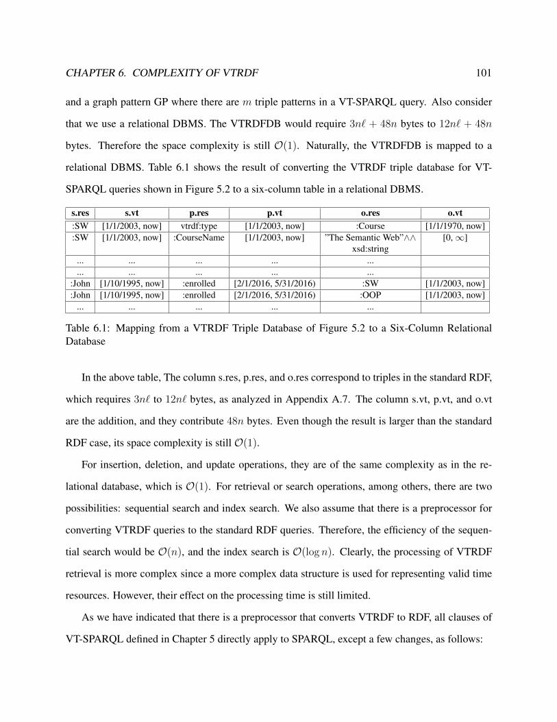
CHAPTER 6. COMPLEXITY OF VTRDF 101
and a graph pattern GP where there are m triple patterns in a VT-SPARQL query. Also consider
that we use a relational DBMS. The VTRDFDB would require 3n` + 48n bytes to 12n` + 48n
bytes. Therefore the space complexity is still O(1). Naturally, the VTRDFDB is mapped to a
relational DBMS. Table 6.1 shows the result of converting the VTRDF triple database for VT-
SPARQL queries shown in Figure 5.2 to a six-column table in a relational DBMS.
s.res s.vt p.res p.vt o.res o.vt:SW [1/1/2003, now] vtrdf:type [1/1/2003, now] :Course [1/1/1970, now]:SW [1/1/2003, now] :CourseName [1/1/2003, now] ”The Semantic Web”∧∧ [0,∞]
xsd:string... ... ... ... ...... ... ... ... ...
:John [1/10/1995, now] :enrolled [2/1/2016, 5/31/2016) :SW [1/1/2003, now]:John [1/10/1995, now] :enrolled [2/1/2016, 5/31/2016) :OOP [1/1/2003, now]
... ... ... ... ...
Table 6.1: Mapping from a VTRDF Triple Database of Figure 5.2 to a Six-Column RelationalDatabase
In the above table, The column s.res, p.res, and o.res correspond to triples in the standard RDF,
which requires 3n` to 12n` bytes, as analyzed in Appendix A.7. The column s.vt, p.vt, and o.vt
are the addition, and they contribute 48n bytes. Even though the result is larger than the standard
RDF case, its space complexity is still O(1).
For insertion, deletion, and update operations, they are of the same complexity as in the re-
lational database, which is O(1). For retrieval or search operations, among others, there are two
possibilities: sequential search and index search. We also assume that there is a preprocessor for
converting VTRDF queries to the standard RDF queries. Therefore, the efficiency of the sequen-
tial search would be O(n), and the index search is O(log n). Clearly, the processing of VTRDF
retrieval is more complex since a more complex data structure is used for representing valid time
resources. However, their effect on the processing time is still limited.
As we have indicated that there is a preprocessor that converts VTRDF to RDF, all clauses of
VT-SPARQL defined in Chapter 5 directly apply to SPARQL, except a few changes, as follows:

CHAPTER 6. COMPLEXITY OF VTRDF 102
• A valid time variable in VT-SPARQL is converted to a resource variable in SPARQL. More-
over, it is allowed to refer to the components of a valid time variable, i.e., the resource part
and the valid time part.
• In regular or arithmetic expressions, references to the resource part and the valid time part
of valid time resources or valid time variables are allowed.
• SameResource in VT-SPARQL expressions are converted to regular expressions in SPARQL,
which compare literal values.
• Temporal predicates in VT-SPARQL can be directly converted to arithmetic expressions in
SPARQL.
The preprocessor would use these rules to convert a VT-SPARQL query to an equivalent
SPARQL query, which is then evaluated against the temporal triple store.
On this basis, we adopt the complexity analysis in [57], which showed that evaluating SPARQL
queries can be solved in time O(mn), where m is the number of triple patterns and n is the
number of triples in the triple database, for a graph pattern formed by using only AND and FILTER
operators. This case is the same as our VT-SPARQL query evaluation based on the analysis of
correspondence between VT-SPARQL and SPARQL. That is, evaluating VT-SPARQL queries can
also be solved in time O(mn). Furthermore, it is also shown in [57] that if the UNION and
OPTION operator are allowed in the graph pattern expressions, the query evaluation becomes NP-
complete and PSPACE-complete.
Even though the complexity of VTRDF entailment is beyond the scope of this thesis, we have a
few observations. As we have indicated that VTRDF is RDF-compliant, the complexity of VTRDF
entailment may resemble the case of the entailment in the standard RDF. That is, both VTRDF
and VTRDFS entailments are NP-Complete. As a hint for further analysis, we observe that in
Temporal RDF [30, 19] that we have surveyed, which incorporated one timestamp into a RDF

CHAPTER 6. COMPLEXITY OF VTRDF 103
triple and used RDF reification, it has been proved that the temporal entailment for temporal RDF
graphs is NP-complete. This outcome the remains the same as the case in the standard RDF
analyzed in Appendix A.7. In other words, the time dimension does not increase the complexity
of non-temporal entailment.

Chapter 7
Conclusions and Future Works
This thesis focuses on modeling binary relations that have the necessity of adding an additional
temporal dimension with the standard RDF, which is a binary-relation-only model. There are
extensive research efforts underway for incorporating temporality into RDF and its variants. For
temporal data models, two attributes of time are usually considered: valid time and transaction
time. As the majority of temporal models reported focus on the valid-time aspect of temporality,
we select valid time as the additional dimension. We therefore investigate proposals of temporal
models of the Semantic Web in the literature. These models mainly extend RDF, RDFS, or OWL
to represent temporal data by either Explicit Reification or Implicit Reification, which are the basis
of a taxonomy, shown in Figure 3.11, that we have developed to classify them. While Explicit
Reification is a method included in the RDF standard, Implicit Reification aims at generating
identity by which additional data can be specified in RDF. We expect that the taxonomy would be a
base for a better understanding of temporal extensions to RDF. Additionally, we have summarized
key characteristics of these models and provided them in Table 3.2. The summary in Table 3.2
would be useful for the researchers and practitioners of the Semantic Web. We envision that RDF,
RDFS or OWL compliant temporal models can be handled and implemented directly, and available
tools, such as triple stores and reasoners can also be used. However, representing temporal data and
104

CHAPTER 7. CONCLUSIONS AND FUTURE WORKS 105
knowledge definitely requires additional triples. The proliferation of triples causes performance,
maintenance and storage issues. A feasible solution would be to reduce the number of additional
triples to a minimum for representing temporal data. Also, this would make writing queries more
intuitive and less complex.
On this basis, we adopt a modeling approach motivated by the 4D view to address the issues we
have observed in the survey. Most proposals we investigated in Chapter 3 concern only one times-
tamp for a given RDF triple. However, we believe that three timestamps should be incorporated
for fully representing temporal knowledge in order to preserve the complete temporal aspect of a
RDF triple. Every resource naturally comes with a valid timestamp that denotes its existence in
time. When two resources coexist in time and form a binary relationship, a factual time is settled.
This is the timestamp that most of the proposals surveyed in Chapter 3 focus on. Altogether, we
observe that three timestamps are necessary for a binary relationship. To materialize the idea, we
come up with the valid time resource, and propose Valid Time RDF, or VTRDF. VTRDF takes the
valid time resource as its first-class citizen. A valid time resource is a RDF-compliant resource
equipped with a valid time that denotes its existence in time. Our approach treats all resources
in VTRDF uniformly, which is significant in that the need of RDF reification is eliminated. In
particular, using VTRDF to handle temporal data and knowledge requires no additional triples or
objects.
To formally represent valid time resources, and construct VTRDF triples and graphs, we extend
the standard IRI to Valid Time IRI, which separates the second fragment identifier by a delimiter
(•) in addition to the first fragment identifier delimited by # of the standard IRI. For time represen-
tation, we employ interval-based timestamps defined in section 4.2, whose unit of time points is
the standard U.S. calendar days in the format of month/day/year. Furthermore, literals, data types,
blank nodes of the standard RDF are all temporalized to their valid time variants. Operations for
valid time resources are carried out by a family of projection functions, which project valid time
resources to various dimensions, such as the resource dimension and the valid time dimension.
CHAPTER 7. CONCLUSIONS AND FUTURE WORKS 106
For convenience, we allow the dot notation (.) to denote a projection to a given dimension. For
instance, vt.res denotes a non-temporal resource part of the valid time resource vt.
A VTRDF triple is defined over qualifying valid time resources. Each VTRDF triple is required
to satisfy the Temporal Triple Integrity given in Definition 4.5.9. For compactness, we confine a
VTRDF graph to strict temporal constraints given in Definition 4.5.11. On top of simple use of
VTRDF, we define layered sets of VTRDF vocabulary and VTRDF Schema vocabulary, which are
the temporal variants of their counterparts in the standard RDF. These new vocabularies are under
the customized namespace prefixed by vtrdf: and vtrdfs: respectively. The formal semantics of
VTRDF is given by the model-theoretic semantics, which uses interpretation models and semantic
conditions for evaluating VTRDF triples and graphs. We also identify useful entailment patterns
for both VTRDF and VTRDF Schema vocabularies.
For querying VTRDF triple databases, we design a query language, Valid Time SPARQL (VT-
SPARQL). As VTRDF differs from the standard RDF, additional requirements are considered in
designing VT-SPARQL. For instance, the representation of valid time resources, time intervals,
and instants are available. Valid time variables are used in VT-SPARQL in correspondence to the
standard variables in SPARQL. Specifically a valid time variable matches to a valid time resource.
Two query forms are considered in VT-SPARQL: SELECT and CONSTRUCT queries. For FIL-
TER conditions used within the WHERE clause, we incorporate Allen’s temporal predicates [4]
for comparing time intervals explicitly. Either a time interval literal, or a bound valid time variable
that has been projected to its valid time part can appear as arguments of the temporal predicates.
We have also provided a set of examples in VT-SPARQL. These examples demonstrate the use
of built-in constructs of VT-SPARQL with an example triple database that originated from the
running example given in Figure 4.3.
In the complexity analysis of VTRDF, we have shown that storing VTRDF triples in a rela-
tional database requires 3n` + 48n bytes to 12n` + 48n bytes where n is the number of triples
in the VTRDF triple database. Even though the space requirement is higher, its space complexity

CHAPTER 7. CONCLUSIONS AND FUTURE WORKS 107
is still O(1). Furthermore, there is no additional object needed for modeling temporal data and
knowledge, and the number of triples remains the same. For insertion, deletion, and update op-
erations, they are of the same time complexity as in the relational database, which is O(1). For
retrieval or search operations, the efficiency of the sequential search would beO(n), and the index
search isO(log n). The processing of VTRDF retrieval is more complex since a more complex data
structure is needed for representing valid time resources. However, their effect on the processing
time is still limited.
We assume a non-native implementation of VTRDF triple database and also a preprocessor.
The complexity of evaluating VT-SPARQL queries therefore resembles the complexity of evalu-
ating SPARQL queries based on their corresponding constructs and changes discussed in chapter
6. Evaluating SPARQL queries can be solved in time O(mn), where m is the number of triple
patterns and n is the number of triples in the triple database, for the graph pattern formed by us-
ing only AND and FILTER operators. Furthermore, it is also shown in [57] that if the UNION
and OPTION operator are allowed in the graph pattern expressions, the query evaluation becomes
NP-complete and PSPACE-complete.
There are several directions that we can further investigate. The majority of temporal models
focuses on the valid time aspect of temporality. However, being able to incorporate other temporal
dimensions, such as transaction time or bitemporal, would allow richer implementation in temporal
semantics of the Semantic Web applications. A top-level time ontology that provides enough
temporal expressive power, and facilitates more powerful temporal reasoning would be highly
desirable too.
In this thesis, we do not address the impact of valid time blank nodes on the semantics of
VTRDF graphs. Valid time blank nodes are used to denote existential resources without specify-
ing their valid time IRIs, and the semantics requires definitions of closure properties of VTRDF
graphs. This extension will allow more VTRDF modeling cases that involve anonymous resources
or timestamps.

CHAPTER 7. CONCLUSIONS AND FUTURE WORKS 108
For VT-SPARQL, we only allow valid time variables and require matching to valid time re-
sources exclusively. We can further open up more query scenarios by allowing two additional
types of variables: standard resource variables and time interval variables. A standard resource
variable would be used in place of the resource part of a valid time resource. It is to bind to a stan-
dard resource provided that their valid time strictly matches. A time interval variable, represented
by two instant variables, which are the beginning and end instants, would be used in place of the
valid time part of a valid time resource. In this way, we will be able to represent an arbitrary valid
time resource by concatenating an arbitrary atemporal resource with a valid timestamp.
Lastly, regarding the implementation, we are looking at available tools and packages, shown
in Table B1 of Appendix B, that are open to customization of our VTRDF triple database and
VT-SPARQL query language. For instance, Protege [51] has been a popular ontology editor and
knowledge management system develop by Stanford Center for Biomedical Informatics Research.
The Valid-Time Temporal Model of [55] surveyed in section 3.4.1 has also contributed a Protege
Plugin and SWRLTab to work with SWRL rules and SQWRL queries. Extending Protege to have
the capability of VTRDF could be a worthwhile effort.

Appendices
109

110
A.1 RDF Definitions
The following definitions provide foundations of RDF model and its semantics.
Definition A.1.1. RDF Resource
A RDF resource, r, is any object that can be identified universally. A RDF resource is denoted
by an IRI, or a local identified for a blank node. We designateR as an infinite set of standard RDF
resources.
Definition A.1.2. International Resource Identifier (IRI)
International Resource Identifier, or IRI [23], is an internet protocol standard that is based on
Uniform Resource Identifier, or URI. IRI allows more characters to be used compared to URI.
In the RDF model, an IRI identifies a resource. For instance, a resource John is identified by an
IRI, http://example.org/RDF-SW#John. The symbol # separates the main name space from the
fragment identifier.
Definition A.1.3. RDF Literal
A RDF literal, l, is used for denoting a concrete value, such as a string, a date, or an integer. A
literal is also a constant and will not change its value. A RDF literal contains either two or three
components [21]:
• A lexical form in an unicode string.
• A data type IRI.
• An optional language tag identified by the IRI, http://www.w3.org/1999/02/22-rdf-syntax-
ns#langString.
For instance, ”1”∧∧xsd:integer denotes an integer 10 by the XML Schema integer type. We desig-
nate L as a set of all RDF literals.
111
Definition A.1.4. RDF Data Type
A RDF data type, d, is used with a RDF literal to represent a concrete value. A data type is
denoted by one or more IRIs and consists of:
• A non-empty set of unicode strings as the lexical space L(d).
• A non-empty value space V(d).
• A lexical-to-value mapping L2V : L(d)→ V(d).
Definition A.1.5. Lexical to Value Mapping function (L2V)
L2V is a partial mapping from the lexical space of RDF literals to the value space V . For a
RDF literal l annotated with a data type d, its value is obtained from the value space by L2V. That
is: L2V (l, d) = v where v ∈ V . The L2V mapping can be one-to-one or many-to-one. As an
example for the later case, XML schema data type xsd:boolean [13] has the type specification as
follows:
• L(d) = {”0”, ”1”, ”T”, ”F”}
• V(d) = {true, flase}
• L2V : {”T”→ true, ”F”→ false, ”1”→ true, ”0”→ false}
Definition A.1.6. RDF Property
Let P be the set of any properties. A RDF property p ∈ P is any binary relation that relates
two logically compatible RDF resources. P include properties that belong to RDF and RDFS
vocabularies, which will be defined in section A.2 and section A.3 respectively.
Definition A.1.7. RDF Blank Node
Let B be a set of blank node, a RDF blank node b ∈ B denotes the existence of a RDF resource
whose IRI is not yet known. b is typically assigned a local identifier which has an effective scope
limited to a local RDF triple database.

112
Definition A.1.8. RDF Triple
A RDF triple is in the form of (s, p, o) where s, p, o are RDF resources defined as follows. They
represent the subject, predicate, and object respectively.
• s ∈ R ∪ B
• p ∈ P
• o ∈ R ∪ B ∪ L
Definition A.1.9. RDF Graph
A RDF graph, G, is a set of RDF triples defined as follows:
G = {(s, p, o)|s ∈ (R∪ B) ∧ p ∈ P ∧ o ∈ (R∪ B ∪ L)} (A.1.1)
Definition A.1.10. Subgraph
A RDF graph H is a subgraph of another RDF graphG if H includes some of the RDF triples
in G. For instance, the RDF graph in Figure A1 is a subgraph of the graph in Figure 2.4. A proper
subgraph is a proper subset of the RDF triples in the graph.
ex:John ex:SWex:enrolled
Figure A1: A RDF Subgraph of the Running Example in Figure 2.4
Definition A.1.11. RDF Graph Vocabulary
Given a RDF graph G and the set of RDF resources R appear in G, the vocabulary voc(G) is
the set of valid IRIs that appear in G excluding RDF literals.

113
Definition A.1.12. Ground RDF Triple and Graph
A ground RDF triple is a RDF triple that does not contain any blank nodes. A ground RDF
graph is therefore a RDF graph that contains only ground RDF triples.
Definition A.1.13. RDF Mapping Function
A mapping function, M : (R∪B∪L)→ (R∪B∪L), maps a RDF resource, a RDF literal, or
a RDF blank node to a RDF resource, a RDF literal, or another RDF blank node. M is defined to
map elements of one RDF graph to another. Four mapping cases at the resource level are defined
for two given RDF graphs Gt1 and Gt
2 as follows:
• M(r1) = r2 where r1 ∈ G1, r2 ∈ G2, and r1 = r2.
• M(l1) = l2 where l1 ∈ G1, l2 ∈ G2, and l1 = l2.
• M(b) = r where b ∈ G1, and r ∈ G2.
• M(b1) = b2 where b1 ∈ G1, and b2 ∈ G2.
In addition, M can be overloaded to map a RDF graph. Given a RDF graph G, M(G) maps to
a set of all (M(s),M(p),M(o) where (s, p, o) ∈ G.
A.2 RDF Vocabulary (rdfV)
The RDF model provides ontological modeling primitives to define terminology vocabularies and
use them for asserting facts. The following set of vocabularies, called RDF vocabulary, or rdfV,
provides more expressive power so that we can model more knowledge for the running example in
Figure 2.4. l
• rdf:Property is the superclass of all properties.

114
• rdf:type is a RDF property to represent instance of relationship between an instance and a
class.
• rdf:Statement is the superclass of all RDF statements.
• rdf:subject, rdf:predicate and rdf:object are RDF properties used to assert the subject, pred-
icate and the object of a RDF statement respectively. They are intended to be used in the
reification. The definition of RDF reification and its implication have been discussed in the
next section.
By using rdfV, additional knowledge about the running example of Figure 2.4 can be expressed.
Figure A2 shows a RDF graph that contains three fresh facts: John is a student, NYC is a city, and
SW is a course.
ex:John
ex:Studentrdf:type
ex:SWex:enrolled
ex:NYC
ex:livedInex:Courserdf:type
ex:Cityrdf:type
Figure A2: Running Example with Additional Facts in RDF Vocabulary (rdfV)
In addition, a set of axioms, shown in Figure A3, follows from the above definitions of vocab-
ularies.

115
PREFIX rdf: <http://www.w3.org/1999/02/22-rdf-syntax-ns#>.
rdf:type rdf:type rdf:Property.
rdf:subject rdf:type rdf:Property.
rdf:predicate rdf:type rdf:Property.
rdf:object rdf:type rdf:Property.
Figure A3: Axioms of RDF Vocabulary (rdfV)
A.3 RDF Schema Vocabulary (rdfsV)
RDF schema, or RDFS, extends RDF vocabulary (rdfV) to allow descriptions of classes, class
taxonomies, and class properties. For RDF properties, their domain and range can also be defined.
Definition A.3.1. RDF Class
A RDF class c is any set of similar resources. Each member is an instance of the class and
defined by using rdf:type assertions. Class hierarchy can also be defined by a subclass relationship.
We designate C as the set of all RDF classes.
RDFS vocabularies are characterized as follows:
• RDF Classes:
– rdfs:Resource is the superclass of all RDF resources.
– rdfs:Literal is the class of all RDF literals.
– rdfs:Class is the the class of all RDF classes.
• RDF Properties:
– rdfs:domain defines the domain of a property. It is also used to define itself.

116
– rdfs:range defines the range of a property. It is also used to define itself.
– rdfs:subClassOf defines the class hierarchy.
– rdfs:subPropertyOf defines the property hierarchy.
A set of axioms in Figure A4, written in Turtle syntax [9], follows from the above definitions
of the RDF classes and properties.
PREFIX rdf: <http://www.w3.org/1999/02/22-rdf-syntax-ns#>.PREFIX rdfs: <http://www.w3.org/2000/01/rdf-schema#>.
rdfs:Class rdfs:subClassOf rdfs:Resource.rdfs:Property rdfs:subClassOf rdfs:Resource.rdfs:Literal rdfs:subClassOf rdfs:Resource.rdf:type rdfs:domain rdfs:Resource.rdf:type rdfs:range rdfs:Class.rdfs:domain rdfs:domain vtrdf:Property.rdfs:domain rdfs:range rdfs:Class.rdfs:range rdfs:domain vtrdf:Property.rdfs:range rdfs:range rdfs:Class.rdfs:subClassOf rdfs:domain rdfs:Class.rdfs:subClassOf rdfs:range rdfs:Class.rdfs:subPropertyOf rdfs:domain vtrdf:Property.rdfs:subPropertyOf rdfs:range vtrdf:Property.
Figure A4: Axioms of RDF Schema Vocabulary (rdfsV)
By using the RDFS classes, class properties and the set of RDFS axioms, inference can be
made. Entailed knowledge can be explicitly added. For instance, the type range axiom in Figure
A4 allows us to infer that the resources ex:Student, ex:Course and ex:City are all range values of
type assertions. Therefore they are RDF classes. The inferred triples are shown in Figure A5 and
we are adding them to the graph of Figure A2 and end up with the updated graph shown in Figure
A6. Please note that the definitions of the inference and entailment will be discussed in the section
A.4.

117
ex:Student rdf:type rdfs:Class.ex:Course rdf:type rdfs:Class.ex:City rdf:type rdfs:Class.
Figure A5: Inferred Triples Based on the Range Axiom in Figure A4
Furthermore, properties about ex:enrolled and ex:livedIn can be asserted by using rdfs:domain
and rdfs:range. In this way, they are defined as terminology vocabularies which are used to assert
facts. Figure A7 shows the complete knowledge base, written in Turtle syntax [9], of the running
example originally described in Figure A2 and Figure A6.
ex:John
ex:Studentrdf:type
ex:SWex:enrolled
ex:NYC
ex:livedInrdfs:Class
rdf:type
ex:Courserdf:type
ex:Cityrdf:type
rdf:typerdf:type
Figure A6: Running Example with Additional Facts in RDF Schema Vocabulary (rdfsV)
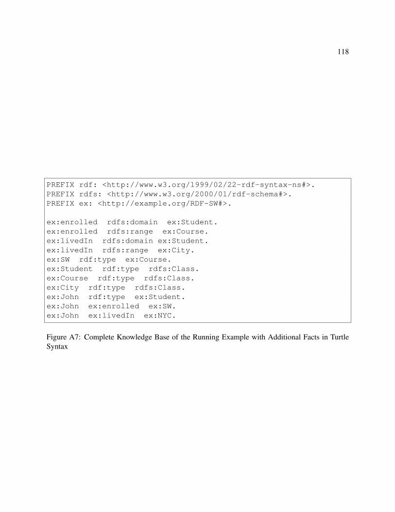
118
PREFIX rdf: <http://www.w3.org/1999/02/22-rdf-syntax-ns#>.PREFIX rdfs: <http://www.w3.org/2000/01/rdf-schema#>.PREFIX ex: <http://example.org/RDF-SW#>.
ex:enrolled rdfs:domain ex:Student.ex:enrolled rdfs:range ex:Course.ex:livedIn rdfs:domain ex:Student.ex:livedIn rdfs:range ex:City.ex:SW rdf:type ex:Course.ex:Student rdf:type rdfs:Class.ex:Course rdf:type rdfs:Class.ex:City rdf:type rdfs:Class.ex:John rdf:type ex:Student.ex:John ex:enrolled ex:SW.ex:John ex:livedIn ex:NYC.
Figure A7: Complete Knowledge Base of the Running Example with Additional Facts in TurtleSyntax

119
A.4 RDF Semantics and Entailment
The RDF model employs model-theoretic semantics to define its formal semantics [36]. A RDF
triple or a RDF graph asserts facts about the world. The world is so situated that makes these
assertions true. In order to evaluate the truth of a RDF triple or a RDF graph, an interpretation
model is needed to specify the semantic conditions about the situated world. An interpretation
model is basically a functional structure that defines how IRIs or literals should be mapped to the
domain of the interpretation.
RDF is formed by layered sets of pre-defined vocabularies. In fact, the base layer hosts simple
vocabulary that essentially allows any vocabularies except pre-defined ones. On top of it, data
types are allowed, and further to RDF vocabulary, or rdfV and RDFS vocabulary or rdfsV. These
layers of vocabularies give increasing expressive power for the RDF model.
In what follows we will characterize RDF model semantics by four groups of vocabularies, and
define formal semantics for each respectively. In each group, an interpretation model is defined
based on the interpretation domain and a set of semantic conditions for its pre-defined vocabularies.
These groups of vocabularies are:
• Simple Vocabulary (V)
V refers to any vocabularies excluding any data type D, rdfV, or rdfsV.
• Simple Vocabulary with Data Type (V-D)
V-D includes the simple vocabulary V and data type D.
• RDF Vocabulary with Data Type D (rdfV-D)
rdfv-D includes the simple vocabulary, data type D, and rdfV defined in section A.2.
• RDFS Vocabulary with Data Type D (rdfsV-D)
rdfsV-D includes the above mentioned vocabularies and rdfsV defined in section A.3, mainly
including: rdfs:Class, rdfs:subClassOf, rdfs:subPropertyOf, rdfs:domain, and rdfs:range.

120
An interpretation model is composed of a domain, mapping functions, and semantic conditions.
Given a RDF graph,E, if there is an interpretation model I that makesE true, we say that I satisfies
E and write I(E) = true. Otherwise E is unsatisfiable. Furthermore, defining an interpretation
model also identifies a certain set of entailment patterns. Entailment, also known as the logical
consequence, describes a satisfaction relationship between statements of logical formulas if one
statement logically follows from one or more statements. Suppose a formula ψ logically follows
from a formula φ. We say that φ entails ψ and write:
φ |= ψ (A.4.1)
The expression (A.4.1) reflects that there exists an interpretation model or truth assignment that
satisfies φ also satisfies ψ. If we consider a RDF graph as a logical formula, the entailment regime
should work similarly for RDF triples and graphs. As we shall see later, for a given vocabulary, we
identify a set of entailment patterns which are on the other hand a set of inference rules. Inference
rules are useful in that given a RDF graph, implicit triples can potentially be derived by applying
appropriate inference rules. In other words, additional knowledge can be inferred and added to the
original RDF graph .
A.4.1 Simple Interpretation
Given a simple vocabulary V, the simple interpretation I is defined as the following components:
• A setR of resources as the domain of I .
• A set P of RDF properties in I .
• A mapping IXT from P toR × R.
• A mapping IS from IRI toR ∪ P .

121
• A partial mapping IL from L toR.
Given a ground RDF triple (s, p, o), I((s, p, o)) is true or satisfiable if all of the following condi-
tions hold:
• s, p, o ∈ V
• IS(p) ∈ P
• < IS(s), IS(o) >∈ IXT(IS(p))
Otherwise, I((s, p, o)) is false. Given a set of triples S, I(S) is true or satisfiable if for every
triple (s, p, o) ∈ S, I((s, p, o)) is true, otherwise I(S) is false or unsatisfiable. We say that I is a
model for S and write I |= S.
A.4.2 Simple Entailment
Given two RDF graphs G1 and G2, a simple entailment pattern can be identified as the subgraph
relationship, which follows the interpolation lemma in the RDF specification [36], as follows:
G simply entails a graph E if and only if a subgraph of G is an instance of E (A.4.2)
As a result, ifG2 is a subgraph ofG1, G1 entailsG2, orG1 |= G2. For instance, the RDF graph,
G1, in Figure A6 entails the graph, G2, in Figure A2 because G2 contains a subset of triples in G1.
A.4.3 Simple-D Interpretation
On top of the simple interpretation, a simple-D interpretation satisfies additional semantic condi-
tions with a set of IRIs that identifies RDF data types, denoted by D. Given the vocabulary V -D,
the simple-D interpretation, I , is defined as the following conditions:
• Any RDF graph that contains ill-typed literals is false or unsatisfiable.

122
• For a RDF literal, l, together with a data type, d, where l ∈ L and d ∈ D, represented as
l∧∧d, its value is defined as:
IL(l∧∧d) = L2V (I(d), l) (A.4.3)
A.4.4 Simple-D Entailment
Given two RDF triples e1 and e2 that contain RDF literals l1 and l2, and data types: d1, d1 respec-
tively, as follows:
e1 = (s, p, l∧∧1 d1)
e2 = (s, p, l∧∧2 d2)
(A.4.4)
e1 entails e2 if and only if L2V (l1, I(d1)) = L2V (l2, I(d2)).
The simple-D entailment pattern holds if both literals l1 and l2 map to the same value under
the lexical-to-value map of the data type in D, regardless of their surface representations. For
instance, the entailment in expression A.4.5 holds as the two typed literals, ”25.0”∧∧xsd:decimal
and ”25”∧∧xsd:decimal map to the same value of xsd:integer in D.
(ex:book1, ex:listPrice, ”25.0”∧∧xsd:decimal) |= (ex:book1, ex:listPrice, ”25”∧∧ xsd:decimal)
(A.4.5)
A.4.5 RDF Interpretation
Given rdfV given in section A.2, a RDF interpretation I is a simple-D interpretation and satisfies
the additional semantic conditions as follows:
1. For a RDF property p ∈ P , (p, I(rdf:Property)) ∈ IXT(I(rdf:type).

123
2. For a RDF literal l and a RDF data type d, (l, I(d)) is in IXT(I(rdf:type) if and only if l is
in the value space of I(d).
3. The set of RDF axiomatic triples given in Figure A3 needs to be satisfied.
A.4.6 RDF Entailment
The first semantic condition given above leads to the following entailment pattern:
Given a RDF graph G and a RDF triple (s, p, o) ∈ G:
G |= (p, rdf:type, rdf:Property) (A.4.6)
For instance, the following triple,
ex:John ex:enrolled ex:SW
entails
:enrolled rdf:type rdf:Property.
A.4.7 RDFS Interpretation
For the RDFS vocabulary, an additional component for mapping the set of RDFS classes, C, of
Definition A.3.1 is needed. A mapping function CIXT maps C to a subset of R. A RDFS inter-
pretation I recognizing D is defined as the following semantic conditions:
1. For a RDF class c ∈ C, its mapping CIXT(c) is a collection of resources r that are of the
same kind, and defined as:
c = {r|(r, t) ∈ IXT (I(rdf : type))} (A.4.7)
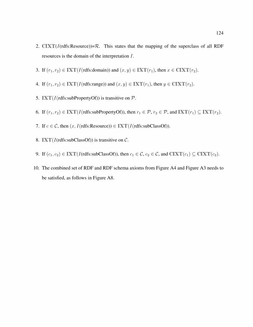
124
2. CIXT(I(rdfs:Resource))=R. This states that the mapping of the superclass of all RDF
resources is the domain of the interpretation I .
3. If (r1, r2) ∈ IXT(I(rdfs:domain)) and (x, y) ∈ IXT(r1), then x ∈ CIXT(r2).
4. If (r1, r2) ∈ IXT(I(rdfs:range)) and (x, y) ∈ IXT(r1), then y ∈ CIXT(r2).
5. IXT(I(rdfs:subPropertyOf)) is transitive on P .
6. If (r1, r2) ∈ IXT(I(rdfs:subPropertyOf)), then r1 ∈ P , r2 ∈ P , and IXT(r1) ⊆ IXT(r2).
7. If c ∈ C, then (x, I(rdfs:Resource)) ∈ IXT(I(rdfs:subClassOf)).
8. IXT(I(rdfs:subClassOf)) is transitive on C.
9. If (c1, c2) ∈ IXT(I(rdfs:subClassOf)), then c1 ∈ C, c2 ∈ C, and CIXT(c1) ⊆ CIXT(c2).
10. The combined set of RDF and RDF schema axioms from Figure A4 and Figure A3 needs to
be satisfied, as follows in Figure A8.

125
PREFIX rdf: <http://www.w3.org/1999/02/22-rdf-syntax-ns#> .PREFIX rdfs: <http://www.w3.org/2000/01/rdf-schema#> .
rdf:type rdf:type rdf:Property.rdf:subject rdf:type rdf:Property.rdf:predicate rdf:type rdf:Property.rdf:object rdf:type rdf:Property.rdfs:Class rdfs:subClassOf rdfs:Resource.rdfs:Property rdfs:subClassOf rdfs:Resource.rdfs:Literal rdfs:subClassOf rdfs:Resource.rdf:type rdfs:domain rdfs:Resource.rdf:type rdfs:range rdfs:Class.rdfs:domain rdfs:domain vtrdf:Property.rdfs:domain rdfs:range rdfs:Class.rdfs:range rdfs:domain vtrdf:Property.rdfs:range rdfs:range rdfs:Class.rdfs:subClassOf rdfs:domain rdfs:Class.rdfs:subClassOf rdfs:range rdfs:Class.rdfs:subPropertyOf rdfs:domain vtrdf:Property.rdfs:subPropertyOf rdfs:range vtrdf:Property.
Figure A8: Combined Set of Axioms of RDF and RDF Schema Vocabulary
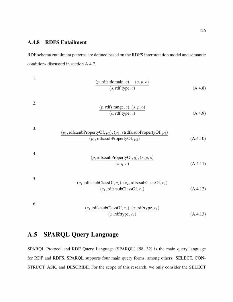
126
A.4.8 RDFS Entailment
RDF schema entailment patterns are defined based on the RDFS interpretation model and semantic
conditions discussed in section A.4.7.
1.(p, rdfs:domain, c), (s, p, o)
(s, rdf:type, c) (A.4.8)
2.(p, rdfs:range, c), (s, p, o)
(o, rdf:type, c) (A.4.9)
3.(p1, rdfs:subPropertyOf, p2), (p2, vtrdfs:subPropertyOf, p3)
(p1, rdfs:subPropertyOf, p3) (A.4.10)
4.(p, rdfs:subPropertyOf, q), (s, p, o)
(s, q, o) (A.4.11)
5.(c1, rdfs:subClassOf, c2), (c2, rdfs:subClassOf, c3)
(c1, rdfs:subClassOf, c3) (A.4.12)
6.(c1, rdfs:subClassOf, c2), (x, rdf:type, c1)
(x, rdf:type, c2) (A.4.13)
A.5 SPARQL Query Language
SPARQL Protocol and RDF Query Language (SPARQL) [58, 32] is the main query language
for RDF and RDFS. SPARQL supports four main query forms, among others: SELECT, CON-
STRUCT, ASK, and DESCRIBE. For the scope of this research, we only consider the SELECT

127
and CONSTRUCT queries. A SPARQL SELECT or CONSTRUCT query is formed by using the
grammar shown in Figure A9.
[PREFIX Prefix1: IRIOfPrefix1][PREFIX ...]{SELECT RDFResourceList | CONSTRUCT {RDFTripleList}}[FROM IRIOfDefaultGraph][FROM NAMED IRIOfNamedGraphList]WHERE{RDFTriplePatternList[FILTER (Expressions)]}[ORDER BY {ASC(orderComparatorList) | DESC(orderComparatorList)}]
Figure A9: The Grammar of SPARQL
1. PREFIX declaration
A SPARQL query starts with an optional PREFIX declaration for substituting any full valid
time IRIs throughout the query. A PREFIX declaration is composed of the prefix itself and
the full IRI that it stands for. In Figure A9, the term Prefix1: stands for IRIOdPrefix1, which
is a full IRI. When more than one prefix declaration is needed, each prefix declaration is
separated by a line break. For instance, Figure A10 shows three prefixes: ex:, rdf:, and rdfs:.
PREFIX rdf: <http://www.w3.org/1999/02/22-rdf-syntax-ns#>PREFIX rdfs: <http://www.w3.org/2000/01/rdf-schema#>PREFIX ex: <http://example.org/RDF-SW#>
Figure A10: PREFIX Declaration in a SPARQL Query Statement
2. SELECT or CONSTRUCT clause
A SELECT query retrieves resources from the RDF triple database. The SELECT clause
defines the query output by itemizing a list of variable bindings or RDF resources, which
correspond to the term RDFResourceList in Figure A9. Each variable or RDF resource in
the list is separated by space if more than one is used. For instance, the SELECT clause

128
Figure A11 contains one RDF resource and two resource variables for the output. Moreover,
the actual output is subject to matches against the RDF triple or graph patterns specified in
the WHERE clause, which will also be defined in this section.
SELECT ex:John ?predicate ?object
Figure A11: A SELECT Clause in a SPARQL Query Statement
In comparison, a CONSTRUCT query outputs a single RDF graph. The CONSTRUCT
clause defines a RDF graph template by a list of standard RDF triples, which correspond to
the term RDFTripleList represented in Figure A9. A RDF graph template is composed of at
least one RDF triple, and each triple is composed of RDF resources or resource variables.
If more than one triple is used, each is delimited by a period (.). For instance, the CON-
STRUCT clause in Figure A12 defines a RDF graph template to form a RDF graph with a
fresh predicate, isA, in place of rdf:type defined in section A.2. Moreover, the actual out-
put is subject to matches against the RDF triple or graph patterns specified in the WHERE
clause, which will also be defined in this section.
CONSTRUCT {?subject ex:isA ?object.}
Figure A12: A CONSTRUCT Clause in a SPARQL Query Statement
3. FROM and FROM NAMED clauses
Both FROM and FROM NAMED clauses are optional. The FROM clause contains a stan-
dard IRI of a default RDF graph to be used for matching triple or graph patterns, which cor-
respond to the term IRIOfDefaultGraph represented in Figure A9. For instance, the FROM
clause in Figure A13 specifies the IRI, http://example.org/RDF-SW/SPARQLDefaultGraph,
of the default RDF graph for the query. The FROM NAMED clause contains a set of stan-
dard IRIs of named graphs to be used for matching RDF triple or graph patterns. More than

129
one named graphs can be specified, and the IRI of each named graph should be separated by
space.
FROM <http://example.org/RDF-SW/SPARQLDefaultGraph>
Figure A13: A FROM Clause in a SPARQL Query Statement
4. WHERE clause
The WHERE clause is mandatory for a SPARQL query. At least one triple pattern is required
in the WHERE clause. A RDF triple pattern is the same as a RDF triple in the form of s p o,
with possibly some or all of the components being a resource variable. Each component is
separated by a space. A resource variable starts with a question mark (?) followed by the
name of the variable. It is used in place of any position of subject, predicate or object to
bind to any RDF resource in the RDF triple database. For instance, given the RDF graph
in Figure 2.4 and a triple pattern, ?s :enrolled :SW, the resource variable, ?s, binds to the
resource :John.
5. FILTER clause
A filter clause is optional within the WHERE clause. It introduces conditions for restricting
output solutions that make the specified conditions true. When more than one filter condition
is used, the logical and (&&) connects individual conditions. Please note that for the purpose
of this search, we do not consider logical or connector in SPARQL. The conditions can be
formed for the following types of variable bindings or values:
(a) Literal values by regular expressions
A regular expression, or regex, is used for comparing literals. Each regular expression
takes two arguments, as follows:
regex(text, pattern) (A.5.1)

130
The first argument text is the bound literal value that can be either an actual literal or a
resource variable bound to a literal in the RDF triple database. The pattern represents a
literal to be compared with the text. The expression returns true if the text matches or
contains the pattern exactly, otherwise it returns false. For instance, the FILTER clause
in Figure A14 use regex to compare a resource variable, ?text, with a pattern, ”The
Semantic Web”. The regex returns true if ?text binds to ”The Semantic Web” exactly in
the RDF triple database. When approximate match is needed, the pattern is affixed with
the symbol ∧. For instance, a bound text ”The Semantic Web” would match the pattern
”∧Semantic”.
FILTER regex(?text, "The Semantic Web")
Figure A14: A FILTER Clause with regex in a SPARQL Query Statement
(b) Numerical values by arithmetic expressions
In SPARQL, arithmetic expressions are used to filter numerical variable bindings via
mathematical comparisons that use greater than (>), greater than equal to (>=), less
than (<), less than equal to (<=), equal to (=), and not equal to (6=). The FILTER clause
in Figure A15 uses a greater than comparison to restrict the RDF resource variable,
?price.
FILTER (?price >100)
Figure A15: A FILTER Clause with an Arithmetic Expression for a SPARQL Query Statement
(c) ORDER BY clause
ORDER BY clause is used to modify the order of the output based on the specified
order comparator list. Each order comparator is composed of a bound resource variable
and an optional order modifier. The order modifier is either ascending, indicated by
ASC(), or descending, indicated DESC(). For instance, in Figure A16, ORDER By

131
DESC(?student) modifies the resource variable, ?student so the output sequence will
appear in a descending order based on the IRI of bound values of ?student.
SELECT ?studentWHERE{ ?student ex:enroll ?course }ORDER BY DESC(?student)
Figure A16: An ORDER BY Modifier in a SPARQL Query Statement
A.6 SPARQL Examples
Now we give SPARQL query examples based on the RDF triple database shown in Figure A17.
The database is taken from Figure A7 along with more triples added for demonstrating each clause
and language component defined in this section. We also reference the database in Figure A17 by
the graph name, H , whose valid time IRI is: http://example.org/RDF-SW/SPARQLDefaultGraph.
For each query example, it is presented in two parts: the query statement and the output, unless
otherwise specified. While the query statement is written in Turtle [9], the output is presented
in a tabular format to avoid using verbose expressions, such as using XML serializations. When
necessary, the output can also be presented by RDF graphs.

132
# RDFGraph: http://example.org/RDF-SW/SPARQLDefaultGraphex:SW rdfex:type ex:Course.ex:SW ex:CourseName"The Semantic Web"ˆˆ xsd:string.ex:SW ex:requiredTextbook ex:book1.ex:book1 ex:title"Introduction to Semantic Web Technology"ˆˆxsd:string.ex:book1 ex:listPrice "149"ˆˆ xsd:integer.ex:OOP rdf:type ex:Course.ex:OOP ex:CourseName "Object-Oriented Programming"ˆˆ xsd:string.ex:OOP ex:requiredTextbook ex:book2.ex:book2 ex:title "Thinking in C++"ˆˆxsd:string.ex:book2 ex:listPrice "99"ˆˆ xsd:integer.ex:Student rdf:type rdfs:Class.ex:undergraduateStudent rdf:type rdfs:Class.ex:graduateStudent rdf:type rdfs:Class.ex:Course rdf:type rdfs:Class.:City rdf:type rdfs:Class.ex:John rdf:type ex:graduateStudent.ex:John ex:enrolled ex:SW.ex:John ex:enrolled ex:OOP.ex:John ex:enrolled ex:DBMS.ex:John ex:livedIn ex:NYC.ex:Alex rdf:type ex:undergraduateStudent.ex:Alex ex:enrolled ex:DBMS.
Figure A17: The RDF Triple Database for SPARQL Query Examples

133
1. Find all triples about John as a subject.
PREFIX ex: <http://example.org/RDF-SW#>
SELECT ex:John ?predicate ?object
FROM <http://example.org/RDF-SW/SPARQLDefaultGraph>
WHERE
{
ex:John ?predicate ?object
}
:John predicate objectex:John rdf:type ex:graduateStudentex:John ex:enrolled ex:SWex:John ex:enrolled ex:OOPex:John ex:enrolled ex:DBMSex:John ex:livedIn ex:NYC
Table A1: Output of SPARQL Query 1: Find all triples about John as a subject
2. Find courses in which John enrolled.
PREFIX ex: <http://example.org/RDF-SW#>
SELECT ?course
FROM <http://example.org/RDF-SW/SPARQLDefaultGraph>
WHERE
{
ex:John ex:enrolled ?course
}

134
courseex:SW
ex:OOP
Table A2: Output of SPARQL Query 2: Find courses in which John enrolled
3. Find the course names in which John enrolled.
PREFIX ex: <http://example.org/RDF-SW#>
SELECT ?name
FROM <http://example.org/RDF-SW/SPARQLDefaultGraph>
WHERE
{
ex:John ex:enrolled ?course.
?course ex:CourseName ?name.
}
name”The Semantic Web”
”Object-Oriented Programming”
Table A3: Output of SPARQL Query 3: Find the course names in which John enrolled

135
4. Find course names that contain the literal ”Semantic”.
PREFIX ex: <http://example.org/RDF-SW#>
SELECT ?name
FROM <http://example.org/RDF-SW/SPARQLDefaultGraph>
WHERE
{
?subject ex:CourseName ?name.
FILTER regex(?name, "ˆSemantic")
}
name”The Semantic Web”
Table A4: Output of SPARQL Query 4: Find course names that contain the literal ”Semantic”
5. Find books that have a list price higher than 100 dollars. Output the literals of book names.
PREFIX ex: <http://example.org/RDF-SW#>.
SELECT ?bookName
FROM <http://example.org/RDF-SW/SPARQLDefaultGraph>
WHERE
{
?book ex:title ?bookName.
?book ex:listPrice ?price.
FILTER (?price > 100)
}
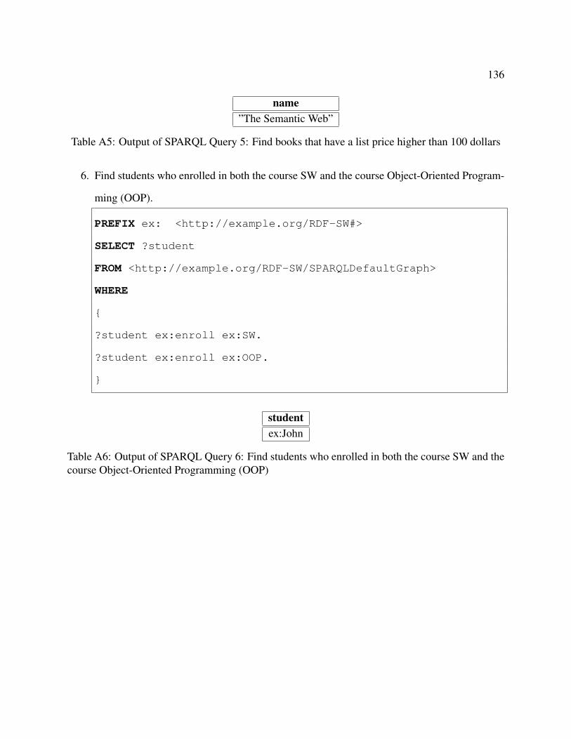
136
name”The Semantic Web”
Table A5: Output of SPARQL Query 5: Find books that have a list price higher than 100 dollars
6. Find students who enrolled in both the course SW and the course Object-Oriented Program-
ming (OOP).
PREFIX ex: <http://example.org/RDF-SW#>
SELECT ?student
FROM <http://example.org/RDF-SW/SPARQLDefaultGraph>
WHERE
{
?student ex:enroll ex:SW.
?student ex:enroll ex:OOP.
}
studentex:John
Table A6: Output of SPARQL Query 6: Find students who enrolled in both the course SW and thecourse Object-Oriented Programming (OOP)

137
7. Find courses that have both undergraduate and graduate students enrolled.
PREFIX ex: <http://example.org/RDF-SW#>
SELECT ?course
FROM <http://example.org/RDF-SW/SPARQLDefaultGraph>
WHERE
{
?student1 rdf:type ex:graduateStudent.
?student1 ex:enrolled ?course.
?student2 rdf:type ex:undergraduateStudent.
?student2 ex:enrolled ?course.
}
studentex:DBMS
Table A7: Output of SPARQL Query 7: Find courses that have both undergraduate and graduatestudents enrolled
8. Construct a RDF graph that contains a new property residentOf whose IRI is:
http://example.org/RDF-SW#residentOf.
PREFIX ex: <http://example.org/RDF-SW#>
CONSTRUCT {ex:John ex:residentOf ?city.}
FROM <http://example.org/RDF-SW/SPARQLDefaultGraph>
WHERE
{ex:John ex:livedIn ?city.}

138
ex:John ex:NYCex:residentOf
Figure A18: Output of SPARQL Query 8: Construct a RDF graph that contains a new propertyresidentOf whose IRI is: http://example.org/Temporal-SW#residentOf

139
A.7 Complexity of RDF
In this section, we discuss its complexity of RDF with respect to space, insertion, deletion, update,
and retrieval queries in SPARQL.
As we have indicated in section 2.4, encoding RDF triples and graphs are achieved by text-
based serializations, such as XML and Turtle [9], which are all Unicode strings. On this basis,
a RDF Triple Store could utilize a storage scheme to assure the performance of database-like
operations, such as retrieval, insertion, update, and deletion of triples, RDF/RDFS entailment, and
SPARQL query execution. In fact, only IRIs, local existential variables, or literals are needed in
storing RDF triples and processing SPARQL queries. An IRI is a Unicode string that conforms
to RFC 3987 [22]. Each character of an IRI may occupy one to four bytes, depending on the
encoding scheme and the allowable character set employed by the storage system. A length ` of an
IRI occupies at most 4` bytes. Hence, the space requirement for one RDF triple is bounded by 12`
bytes (i.e., 4` bytes for each of the subject, predicate, and object). A RDF triple store containing n
triples would require 3n` to 12n` bytes. Therefore the space complexity is O(1).
In [15], a taxonomy of the RDF implementation identifies two main approaches: non-native
implementation and native implementation. The non-native implementation mostly stores RDF
triples and graphs in a Database Management System (DBMS) by converting RDF schema to a
target database schema, such as the relational model. In comparison, the native implementation
does not use any existing DBMS, but implement its own storage and indexing solutions.
Consider a non-native storage approach, a RDF triple database, or RDFDB, which contains
n triples, and a graph pattern GP where there are m triple patterns. Also consider that we use a
relational database, the RDFDB is mapped to a three-column table stored in a relational DBMS.
For instance, the triple store shown in Figure A17 is mapped to the three-column table shown in
Table A8. Clearly, its space complexity is O(1) it requires 3n` to 12n` bytes.
For insertion, deletion, and update operations, they are of the same in time efficiency as in the

140
Subject Predicate Object:SW rdf:type :Course:SW :CourseName ”The Semantic Web”∧∧xsd:string
... ... ...
... ... ...:John :enrolled :SW:John :enrolled :OOP
... ... ...
Table A8: Mapping from a RDF Triple Database of Figure A17 to a Three-Column RelationalDatabase
relational database, which is the O(1). For retrieval or search operations, among others, we may
consider two possibilities: sequential search and index search. The efficiency of the sequential
search would be O(n), and the index search is O(log n).
The complexity of evaluating SPARQL queries has been proved O(mn) [57] where n is the
number of triples and m is the number of triple patterns in a graph pattern, for the graph pattern
constructed by using only AND and FILTER operators. Furthermore, if the UNION operator is
allowed in the graph pattern expressions, the evaluation is NP-complete and PSPACE-complete.
For query evaluation, we can follow the previous two cases, native and non-native approaches. In
the non-native implementation, storing RDF graphs in a relational database benefits from query
optimization available in a relational DBMS. In the case of the native storage approach, the data
structure may be more efficient since there is no overhead needed for the relational DBMS. Prob-
ably its space efficiency is comparable to the non-native case, if not better. However, the main
drawback is that the whole system needs to be implemented from scratch, which is expensive and
time consuming.
In the previous sections, four levels of RDF entailments: simple, simple-D, RDF, and RDFS
entailments, are discussed. The complexity of these entailments are well known, and have been
proved NP-Complete via the equivalence with Graph Homomorphism [31], a reduction to a Clique
problem [69], or a graph coloring problem [68]. A polynomial case is possible when the target

141
graph of the entailment problem is a ground RDF graph [69]. The proof of entailment is beyond
the scope of this thesis.

142B.1 Summary of RDF and RDFS Tools and Packages
Category \ Tool Protege Jena Sesame SWIProlog AllegroGraph ClioPartria BigData Oracle Semantic Turkey RDFLib RDFSharp
Development Y Y YParser Y Y YAPI Y Y Y YTripleStore Y Y Y Y Y Y YReasoner Y Y Y Y Y Y YRDFS Reasoner Y Y Y YRule Reasoner Y YVisualizer Y YProgramming Y Y Y Y Y Y Y
Table B1: Summary of RDF and RDFS Tools

143
• Protege: free, an open source ontology editor and knowledge management system.
• Jena: free and open source Java framework for building Semantic Web and Linked Data
applications.
• Sesame: open-source framework for querying and analyzing RDF data with Java API.
• SWIProlog: open source implementation of the programming language Prolog–interfacing
to RDF/RDFS.
• AllegroGraph: closed source triplestore; currently in use in Open source projects, commer-
cial projects and Department of Defense projects.
• BigData: standards-based, high-performance, scalable, open-source graph database, written
entirely in Java.
• Oracle: open, standards-based, scalable, secure, reliable and performant RDF management
platform
• Semantic Turkey: free, extensible, open source Knowledge Management and Acquisition
tool, written in Java and deployed as a Firefox extension
• RDFLib: Python library for working with RDF, a simple yet powerful language for repre-
senting information
• RDFSharp: lightweight C# framework designed to ease the creation of .NET applications
based on the RDF model
Bibliography
[1] IANA-Managed Reserved Domains. https://www.iana.org/domains/
reserved.
[2] Merriam-webster.com. https://www.merriam-webster.com/dictionary/
knowledge. Accessed: 2020-01-06.
[3] Wikipedia: Manual of style/layout. https://en.wikipedia.org/wiki/
Wikipedia:Manual_of_Style/Layout.
[4] ALLEN, J. F. Maintaining Knowledge about Temporal Intervals. Communication of the ACM
26 (November 1983), 832–843.
[5] BARATIS, E., PETRAKIS, E. G., BATSAKIS, S., MARIS, N., AND PAPADAKIS, N. TOQL:
temporal ontology querying language. In International Symposium on Spatial and Temporal
Databases (2009), Springer, pp. 338–354.
[6] BATSAKIS, S., AND PETRAKIS, E. G. Representing Temporal Knowledge in the Seman-
tic Web: the Extended 4d Fluents Approach. In Combinations of Intelligent Methods and
Applications. Springer, 2011, pp. 55–69.
[7] BATSAKIS, S., PETRAKIS, E. G., TACHMAZIDIS, I., AND ANTONIOU, G. Temporal Rep-
resentation and Reasoning in OWL 2. Semantic Web 8, 6 (2017), 981–1000.
144

BIBLIOGRAPHY 145
[8] BECKETT, D. RDF 1.1 N-Triples. World Wide Web Consortium, Recommendation (2014).
[9] BECKETT, D., BERNERS-LEE, T., PRUDHOMMEAUX, E., AND CAROTHERS, G. RDF 1.1
Turtle. World Wide Web Consortium (2014).
[10] BENCH-CAPON, T. Knowledge Representation: An Approach to Artificial Intelligence,. The
APIC SERIES 32. Academic Press, 1990.
[11] BERNERS-LEE, T., AND CONNOLLY, D. Notation3 (N3): A Readable RDF Syntax. W3C
team submission 28 (2011).
[12] BERNERS-LEE, T., HENDLER, J., AND LASSILA, O. The Semantic Web. Scientific Ameri-
can 284, 5 (2001), 34–43.
[13] BIRON, P. V., MALHOTRA, A., CONSORTIUM, W. W. W., ET AL. XML Schema part 2:
Datatypes, 2004.
[14] BIZER, C., CYGANIAK, R., GAUSS, T., AND MARESCH, O. The TriQL. P browser: Filter-
ing information using context-, content-and rating-based trust policies. In Proceedings of the
Semantic Web and Policy Workshop, held in conjunction with the 4th International Semantic
Web Conference (2005), vol. 7, pp. 12–20.
[15] BLIN, G., CURE, O., AND FAYE, D. C. A Survey of RDF Storage Approaches. Revue
Africaine de la Recherche en Informatique et Mathematiques Appliquees 15 (2012).
[16] BRICKLEY, D., GUHA, R. V., AND MCBRIDE, B. RDF Schema 1.1. W3C recommendation
25 (2014), 2004–2014.
[17] CAROTHERS, G. RDF 1.1 N-Quads: A Line-based Syntax for RDF Datasets. W3C Recom-
mendation (2014).

BIBLIOGRAPHY 146
[18] CARROLL, J. J., BIZER, C., HAYES, P., AND STICKLER, P. Named graphs. Web Semantics:
Science, Services and Agents on the World Wide Web 3, 4 (2005), 247–267.
[19] CLAUDIO GUTIERREZ, C. A. H., AND VAISMAN, A. Introducing Time into RDF. IEEE
Trans. on Knowledge and Data Engineering 19 (February 2007), 207–218.
[20] CONSORTIUM, W. W. W., ET AL. RDF 1.1 Concepts and Abstract Syntax. W3C recommen-
dation (2014).
[21] CYGANIAK, R., WOOD, D., LANTHALER, M., KLYNE, G., CARROLL, J. J., AND
MCBRIDE, B. RDF 1.1 Concepts and Abstract Syntax. W3C recommendation 25, 02 (2014).
[22] DUERST, M., AND SUIGNARD, M. RFC 3987: Internationalized Resource Identifiers (IRIs).
IETF, January (2005).
[23] DURST, M., AND SUIGNARD, M. Internationalized Resource Identifiers (IRIs). Tech. rep.,
RFC 3987, January, 2005.
[24] ERMOLAYEV, V., BATSAKIS, S., KEBERLE, N., TATARINTSEVA, O., AND ANTONIOU,
G. Ontologies of Time: Review and Trends. International Journal of Computer Science &
Applications 11, 3 (2014).
[25] FILLMORE, C. J., JOHNSON, C. R., AND PETRUCK, M. R. Background to framenet. In-
ternational journal of lexicography 16, 3 (2003), 235–250.
[26] GADIA, S. K., AND YEUNG, C.-S. A eneralized odel for a relational temporal database.
ACM SIGMOD Record 17, 3 (1988), 251–259.
[27] GALTON, A. Operators vs. Arguments: The ins and outs of reification. Synthese 150, 3
(2006), 415–441.

BIBLIOGRAPHY 147
[28] GANGEMI, A., AND PRESUTTI, V. A multi-dimensional comparison of ontology design
patterns for representing n-ary relations. In SOFSEM (2013), vol. 13, Springer, pp. 86–105.
[29] GRUBER, T. Towards principles for the design of ontologies used for knowledge sharing. In
Formal Ontology in Conceptual Analysis and Knowledge Representation, N. GUARINO and
R. POLI, Eds. Kluwer, 1994.
[30] GUTIERREZ, C., HURTADO, C., AND VAISMAN, A. Temporal RDF. In European Semantic
Web Conference (2005), Springer, pp. 93–107.
[31] GUTIERREZ, C., HURTADO, C. A., MENDELZON, A. O., AND PEREZ, J. Foundations of
Semantic Web Databases. Journal of Computer and System Sciences 77, 3 (2011), 520–541.
[32] HARRIS, S., SEABORNE, A., AND PRUDHOMMEAUX, E. SPARQL 1.1 Query Language.
W3C Recommendation 21 (2013).
[33] HARTIG, O., AND THOMPSON, B. Foundations of an Alternative Approach to Reification
in RDF. arXiv preprint arXiv:1406.3399 (2014).
[34] HAWLEY, K. Temporal parts. Stanford Encyclopedia of Philosophy (2008).
[35] HAYES, P. J. The Second Naive Physics Manifesto.
[36] HAYES, P. J., AND PATEL-SCHNEIDER, P. F. RDF 1.1 Semantics. W3C recommendation
25 (2014), 7–13.
[37] HOBBS, J. R., AND PAN, F. An OWL Ontology of Time. Disponıvel na Internet em
http://www. isi. edu/pan/time/owl-time-july04. txt. Visitado em 15, 06 (2004), 2009.
[38] HOFFART, J., SUCHANEK, F. M., BERBERICH, K., AND WEIKUM, G. YAGO2: A spatially
and temporally enhanced knowledge base from Wikipedia. Artificial Intelligence 194 (2013),
28–61.

BIBLIOGRAPHY 148
[39] HORROCKS, I. OWL: A Description Logic Based Ontology Language. In ICLP (2005),
vol. 3668, Springer, pp. 1–4.
[40] HORROCKS, I., PATEL-SCHNEIDER, P. F., BOLEY, H., TABET, S., GROSOF, B., DEAN,
M., ET AL. SWRL: A semantic web rule language combining OWL and RuleML. W3C
Member submission 21 (2004), 79.
[41] HURTADO, C. A., AND VAISMAN, A. A. Reasoning with Temporal Constraints in RDF. In
PPSWR (2006), pp. 164–178.
[42] JENSEN, C. S., DYRESON, C. E., BOHLEN, M., CLIFFORD, J., ELMASRI, R., GADIA,
S. K., GRANDI, F., HAYES, P., JAJODIA, S., KAFER, W., ET AL. The consensus glossary
of temporal database concepts. In Temporal Databases: Research and Practice. Springer,
1998, pp. 367–405.
[43] KILGARRIFF, A. Wordnet: An electronic lexical database, 2000.
[44] LOPES, N., POLLERES, A., STRACCIA, U., AND ZIMMERMANN, A. AnQL: SPARQLing
Up Annotated RDFS. In International Semantic Web Conference (2010), Springer, pp. 518–
533.
[45] LUTZ, C. Adding numbers to the SHIQ description logic–First results. In IN PROCEED-
INGS OF THE EIGHTH INTERNATIONAL CONFERENCE ON PRINCIPLES OF KNOWL-
EDGE REPRESENTATION AND REASONING (KR2002 (2001), Citeseer.
[46] MCCARTHY, J. Situations, Actions, and Causal Laws. Tech. rep., STANFORD UNIV CA
DEPT OF COMPUTER SCIENCE, 1963.
[47] MCCARTHY, J., ET AL. Programs with Common Sense. RLE and MIT Computation Center,
1960.

BIBLIOGRAPHY 149
[48] MCCARTHY, J., AND HAYES, P. J. Some Philosophical Problems from the Standpoint of
Artificial Intelligence. Readings in artificial intelligence (1969), 431–450.
[49] MILEA, V., FRASINCAR, F., AND KAYMAK, U. tOWL: a Temporal Web Ontology Lan-
guage. IEEE Transactions on Systems, Man, and Cybernetics, Part B (Cybernetics) 42, 1
(2012), 268–281.
[50] MOTIK, B., PATEL-SCHNEIDER, P. F., AND PARSIA, B. OWL 2 Web Ontology Language
Structural Specification and Functional-Style Syntax. W3C Recommendation (2012).
[51] MUSEN, M. A. The protege project: a look back and a look forward. AI Matters 1, 4 (2015),
4–12.
[52] NGUYEN, V., BODENREIDER, O., AND SHETH, A. Don’t like RDF reification? Making
Statements about Statements Using Singleton Property. In Proceedings of the 23rd Interna-
tional Conference on World Wide Web (2014), ACM, pp. 759–770.
[53] NOY, N., RECTOR, A., HAYES, P., AND WELTY, C. Defining n-ary relations on the seman-
tic web. W3C Working Group Note 12, 4 (2006).
[54] O’CONNOR, M., AND DAS, A. SQWRL: a query language for OWL. In Proceedings of
the 6th International Conference on OWL: Experiences and Directions-Volume 529 (2009),
CEUR-WS. org, pp. 208–215.
[55] O’CONNOR, M., AND DAS, A. A Method for Representing and Querying Temporal Infor-
mation in OWL. In Biomedical Engineering Systems and Technologies, Communications in
Computer and Information Science (2011), Springer.
[56] PARSIA, B., AND SIRIN, E. Pellet: An OWL DL Reasoner. In Third International Semantic
Web Conference-Poster (2004), vol. 18.

BIBLIOGRAPHY 150
[57] PEREZ, J., ARENAS, M., AND GUTIERREZ, C. Semantics and Complexity of SPARQL. In
International semantic web conference (2006), Springer, pp. 30–43.
[58] PRUD, E., SEABORNE, A., ET AL. SPARQL Query Language for RDF. W3C Recommen-
dation (2006).
[59] PUGLIESE, A., UDREA, O., AND SUBRAHMANIAN, V. Scaling RDF with Time. In Pro-
ceedings of the 17th international conference on World Wide Web (2008), ACM, pp. 605–614.
[60] ROUCES, J., DE MELO, G., AND HOSE, K. Framebase: Representing n-ary relations using
semantic frames. In European Semantic Web Conference (2015), Springer, pp. 505–521.
[61] SCHILD, K. A correspondence theory for terminological logics: Preliminary report. Techn.
Univ., 1991.
[62] SCHUELER, B., SIZOV, S., STAAB, S., AND TRAN, D. T. Querying for Meta Knowledge. In
Proceedings of the 17th international conference on World Wide Web (2008), ACM, pp. 625–
634.
[63] SIDER, T. Four-dimensionalism: An ontology of persistence and time. Oxford University
Press on Demand, 2001.
[64] STICKLER, P. RDFQ, 2004.
[65] SUCHANEK, F. M., KASNECI, G., AND WEIKUM, G. Yago: a core of semantic knowl-
edge. In Proceedings of the 16th international conference on World Wide Web (2007), ACM,
pp. 697–706.
[66] TANSEL, A. U. Effecient Management of Temporal Knowledge. US Patent No.
US10055450B1 (2018).

BIBLIOGRAPHY 151
[67] TAPPOLET, J., AND BERNSTEIN, A. Applied Temporal RDF: Efficient Temporal Query-
ing of RDF Data with SPARQL. In European Semantic Web Conference (2009), Springer,
pp. 308–322.
[68] TER HORST, H. J. Extending the RDFS Entailment Lemma. In International Semantic Web
Conference (2004), Springer, pp. 77–91.
[69] TER HORST, H. J. Completeness, Decidability and Complexity of Entailment for RDF
Schema and a Semantic Extension Involving the OWL Vocabulary. Journal of web semantics
3, 2-3 (2005), 79–115.
[70] TSARKOV, D., AND HORROCKS, I. Fact++ description logic reasoner: System description.
In International Joint Conference on Automated Reasoning (2006), Springer, pp. 292–297.
[71] UDREA, O., RECUPERO, D. R., AND SUBRAHMANIAN, V. Annotated rdf. ACM Transac-
tions on Computational Logic (TOCL) 11, 2 (2010), 10.
[72] WANG, H.-T., AND TANSEL, A. Temporal Extensions to RDF. Journal of Web Engineering
18 (2019), 125–168.
[73] WELTY, C., FIKES, R., AND MAKARIOS, S. A reusable ontology for fluents in OWL. In
FOIS (2006), vol. 150, pp. 226–236.
[74] WIKIPEDIA CONTRIBUTORS. Moore’s law. [Online; accessed 13-Dec-2019].
[75] WIKIPEDIA CONTRIBUTORS. New york city. [Online; accessed 26-Feb-2020].
[76] WIKIPEDIA CONTRIBUTORS. Boolean satisfiability problem — Wikipedia, the free
encyclopedia. https://en.wikipedia.org/w/index.php?title=Boolean_
satisfiability_problem&oldid=966122596, 2020. [Online; accessed 13-July-
2020].

BIBLIOGRAPHY 152
[77] WIKIPEDIA CONTRIBUTORS. Expert system — Wikipedia, the free encyclope-
dia. https://en.wikipedia.org/w/index.php?title=Expert_system&
oldid=960553186, 2020. [Online; accessed 4-July-2020].
[78] WIKIPEDIA CONTRIBUTORS. Knowledge-based systems — Wikipedia, the free
encyclopedia. https://en.wikipedia.org/w/index.php?title=
Knowledge-based_systems&oldid=954037818, 2020. [Online; accessed
13-July-2020].
[79] ZIMMERMANN, A., LOPES, N., POLLERES, A., AND STRACCIA, U. A general framework
for representing, reasoning and querying with annotated semantic web data. Web Semantics:
Science, Services and Agents on the World Wide Web 11 (2012), 72–95.