* Kay-Uwe Schober, Dipl. Eng. Univ. BDB, Schober + Partner, Am Kuhlenweg 26, D – 44227 Dortmund;University of Dortmund, Faculty 10, Chair of Structural Design, August-Schmidt-Str. 8, D – 44227 Dortmund

Numerical Simulation of Contact Problems –

Traditional Timber Joints under monotonous loading

Kay-Uwe Schober, Dipl. Eng. Univ. BDB

Dresden University of Technology, Germany

Schober + Partner Architects, Lichtenstein / Dortmund, Germany

Summary:

A numerical simulation on rafter–tie beam–connections in traditional roofs under monotonous

loading is presented. A comparison was made to tests performed at Dresden University of

Technology (DE). A step-by-step procedure was adopted to simulate the semi–rigid behaviour

of the connection with point–to–surface contact elements. The results show good correspon-

dence with typical material characteristics. To increase the load carrying capacity further

studies with fibreglass fabrics reinforced joints were considered.

Keywords:

Numerical simulation, Finite-Element Modelling, Contact Problems, Timber Engineering,

Timber Joints, ANSYS

– 2 –

1 Introduction

Connections and joints for timber members can be built conceptually in three ways:

1. With notches, lap joints and mortise–and tenon–joints that transfer the stress

directly from member to member, with the possibility of wooden dowels or pegs to

provide stability. These timber joints are often found in historical structures.

2. With steel or iron mechanical fasteners, such as nails, screws and bolts that transfer

the stress usually by shear through the fastener from one member to the other.

3. With steel connectors, such as plates and especially shaped steel supports (joist

hangers, column bases, framing anchors) that transfer the load from one member to

the other through the metal and the fasteners that secure the metal piece to the

timber member.

Nowadays, timber joints are connected almost exclusively with the last two systems, and a

large number of proprietary plates and metal supports exists. But in recent years it has become

more and more important to know the realistic load carrying capacity of traditional timber

joints for reconstruction, rebuilding and improvement of the structural behaviour.

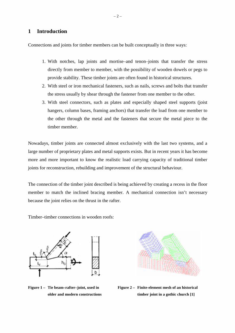
The connection of the timber joint described is being achieved by creating a recess in the floor

member to match the inclined bracing member. A mechanical connection isn’t necessary

because the joint relies on the thrust in the rafter.

Timber–timber connections in wooden roofs:

Figure 1 – Tie beam–rafter–joint, used in Figure 2 – Finite-element mesh of an historical

older and modern constructions timber joint in a gothic church [1]

– 3 –

2 Modelling

2.1 Material properties of used timber

Wood is a cellular organic material from which timber is cut for construction purposes. The

tubular cells of timber have an orientation that gives different properties, depending on the

direction of the grain, and produce a highly anisotropic material (i. e. having different

properties in different directions). This explains why timber is subject to different permissible

stresses depending upon whether the direction of loading is parallel or perpendicular to the

grain.

The strength and elastic properties are designated according to the two principal axes of tim-

ber, parallel or perpendicular to the grain with a high ratio of stiffness and strength between

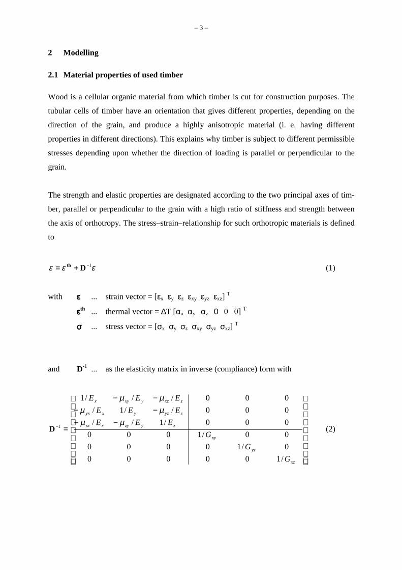
the axis of orthotropy. The stress–strain–relationship for such orthotropic materials is defined

to

εεε 1−+= Dth (1)

with εεεε ... strain vector = [εx εy εz εxy εyz εxz] T

εεεεth ... thermal vector = ∆T [αx αy αz 0 0 0] T

σσσσ ... stress vector = [σx σy σz σxy σyz σxz] T

and D-1 ... as the elasticity matrix in inverse (compliance) form with

−−−−−−

=−

xz

yz

xy

zyzyxzx

zyzyxyx

zxzyxyx

G

G

G

EEE

EEE

EEE

/100000

0/10000

00/1000

000/1//

000//1/

000///1

1µµ

µµµµ

D (2)

– 4 –

and the elastic parameters for the used softwood [2][3][4]

Ex = 13,800 MPa Gxy = 730 MPa

Ey = 910 MPa Gyz = 710 MPa

µxy = 0.02 ρ = 4.80 t/m³

µyz = 0.40 ν = 0.20

2.2 Behaviour of used elements

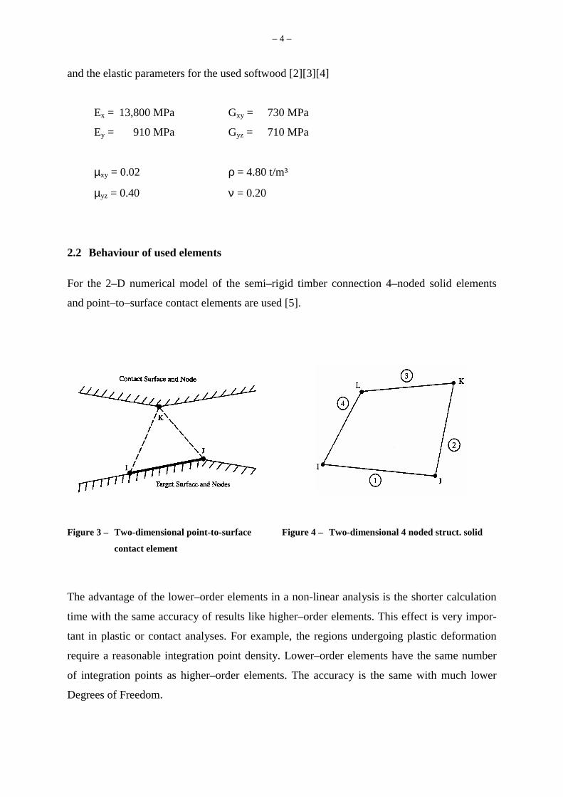
For the 2–D numerical model of the semi–rigid timber connection 4–noded solid elements

and point–to–surface contact elements are used [5].

Figure 3 – Two-dimensional point-to-surface Figure 4 – Two-dimensional 4 noded struct. solid

contact element

The advantage of the lower–order elements in a non-linear analysis is the shorter calculation

time with the same accuracy of results like higher–order elements. This effect is very impor-

tant in plastic or contact analyses. For example, the regions undergoing plastic deformation

require a reasonable integration point density. Lower–order elements have the same number

of integration points as higher–order elements. The accuracy is the same with much lower

Degrees of Freedom.

– 5 –

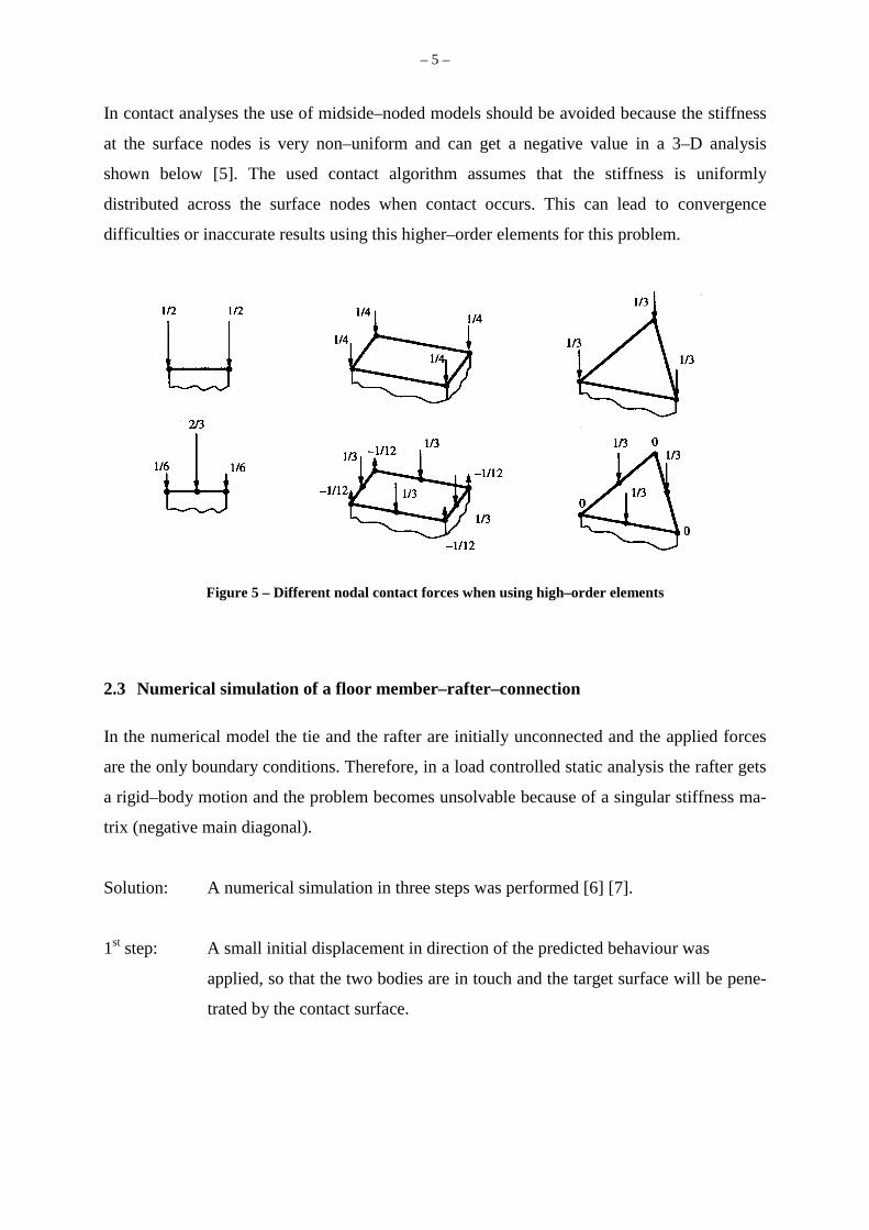
In contact analyses the use of midside–noded models should be avoided because the stiffness

at the surface nodes is very non–uniform and can get a negative value in a 3–D analysis

shown below [5]. The used contact algorithm assumes that the stiffness is uniformly

distributed across the surface nodes when contact occurs. This can lead to convergence

difficulties or inaccurate results using this higher–order elements for this problem.

Figure 5 – Different nodal contact forces when using high–order elements

2.3 Numerical simulation of a floor member–rafter–connection

In the numerical model the tie and the rafter are initially unconnected and the applied forces

are the only boundary conditions. Therefore, in a load controlled static analysis the rafter gets

a rigid–body motion and the problem becomes unsolvable because of a singular stiffness ma-

trix (negative main diagonal).

Solution: A numerical simulation in three steps was performed [6] [7].

1st step: A small initial displacement in direction of the predicted behaviour was

applied, so that the two bodies are in touch and the target surface will be pene-

trated by the contact surface.

– 6 –

The use of weak springs is not recommended because in a large deformation

analysis the results are highly effected by the value of the spring parameter.

The stiffness should be negligible compared to the material stiffness, so that it

has no effect on the solution but the result is a very unstable system.

2nd step: The imposed displacements have been deleted and the reaction forces have

been applied in equal load steps. The structure is still in contact and the stresses

are calculated to zero (starting point).

3rd step: The design load has been applied. The contact and system stiffness of the

rafter has a nonzero value when starting the solution.

⇒ no contact failure, well conditioned system stiffness matrix

Another way to describe the connection is to couple the DOF in the contact zone. The tested

timber joint works only in compression so that the numerical problem becomes non-linear.

During the solution steps the nodal co-ordinate systems do not rotate with the nodes, so that

any coupling equations always act in the original directions. Therefore coupling effects should

be avoided in geometrically non-linear analyses.

2.4 Determination of the Contact Stiffness

In order to handle a contact analysis with the Finite–Element Method it is necessary to estab-

lish a stiffness relationship between the two contact areas. The contact stiffness is used to

enforce compatibility between the contacting surfaces. The contact conditions are described

as a mathematical function with several additional contact terms. The equations in the

simplest form are:

Node–to–Node Contact 0guGg 0T =+= (3)

Node–to–Surface Contact 0g)u(u ng 0targcont ≥+−= (4)

– 7 –

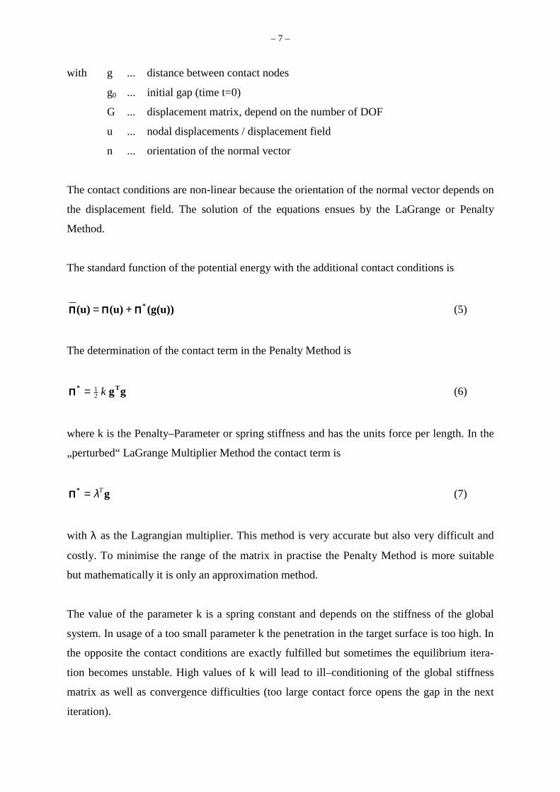
with g ... distance between contact nodes

g0 ... initial gap (time t=0)

G ... displacement matrix, depend on the number of DOF

u ... nodal displacements / displacement field

n ... orientation of the normal vector

The contact conditions are non-linear because the orientation of the normal vector depends on

the displacement field. The solution of the equations ensues by the LaGrange or Penalty

Method.

The standard function of the potential energy with the additional contact conditions is

(g(u))(u)(u) *ΠΠΠΠΠΠΠΠΠΠΠΠ += (5)

The determination of the contact term in the Penalty Method is

gg T* k 21=ΠΠΠΠ (6)

where k is the Penalty–Parameter or spring stiffness and has the units force per length. In the

„perturbed“ LaGrange Multiplier Method the contact term is

g* Tλ=ΠΠΠΠ (7)

with λ as the Lagrangian multiplier. This method is very accurate but also very difficult and

costly. To minimise the range of the matrix in practise the Penalty Method is more suitable

but mathematically it is only an approximation method.

The value of the parameter k is a spring constant and depends on the stiffness of the global

system. In usage of a too small parameter k the penetration in the target surface is too high. In

the opposite the contact conditions are exactly fulfilled but sometimes the equilibrium itera-

tion becomes unstable. High values of k will lead to ill–conditioning of the global stiffness

matrix as well as convergence difficulties (too large contact force opens the gap in the next

iteration).

– 8 –

For an estimation of the value of the local stiffness a safety but a expensive method is to apply

a load to both contact bodies and calculate the corresponding displacements in a linear single–

iteration analysis:

21

1x 100 ... 1

uuk

+= (8)

If the bodies are initially unconnected no local or global system stiffness is available. To cal-

culate the Penalty Parameter the following proposal is made:

− estimation of the resulting forces Fres in direction perpendicular to the contact surface

− estimation of the number of nodes Nc are finally in contact

− determination of the maximum penetration in the contact zone

The contact stiffness will be calculated to

max uN

Fk

c

res= (9)

The maximum of penetration should be approximately 1 % of the characteristic element

length.

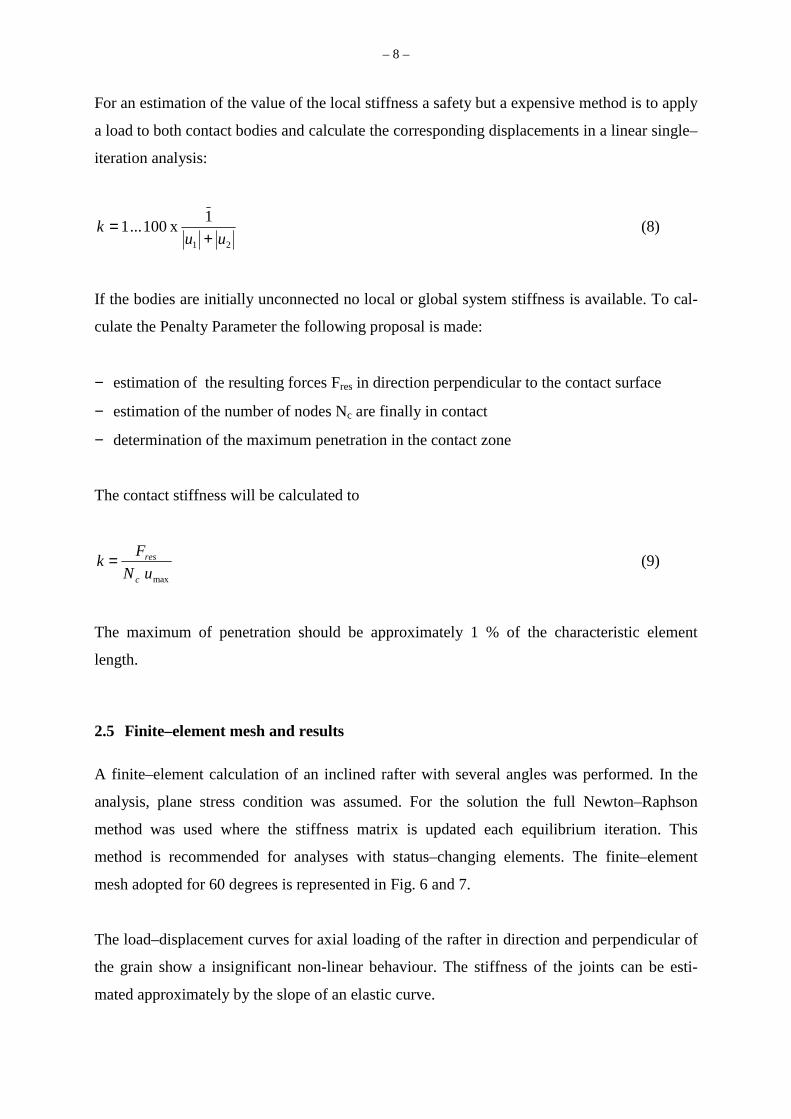
2.5 Finite–element mesh and results

A finite–element calculation of an inclined rafter with several angles was performed. In the

analysis, plane stress condition was assumed. For the solution the full Newton–Raphson

method was used where the stiffness matrix is updated each equilibrium iteration. This

method is recommended for analyses with status–changing elements. The finite–element

mesh adopted for 60 degrees is represented in Fig. 6 and 7.

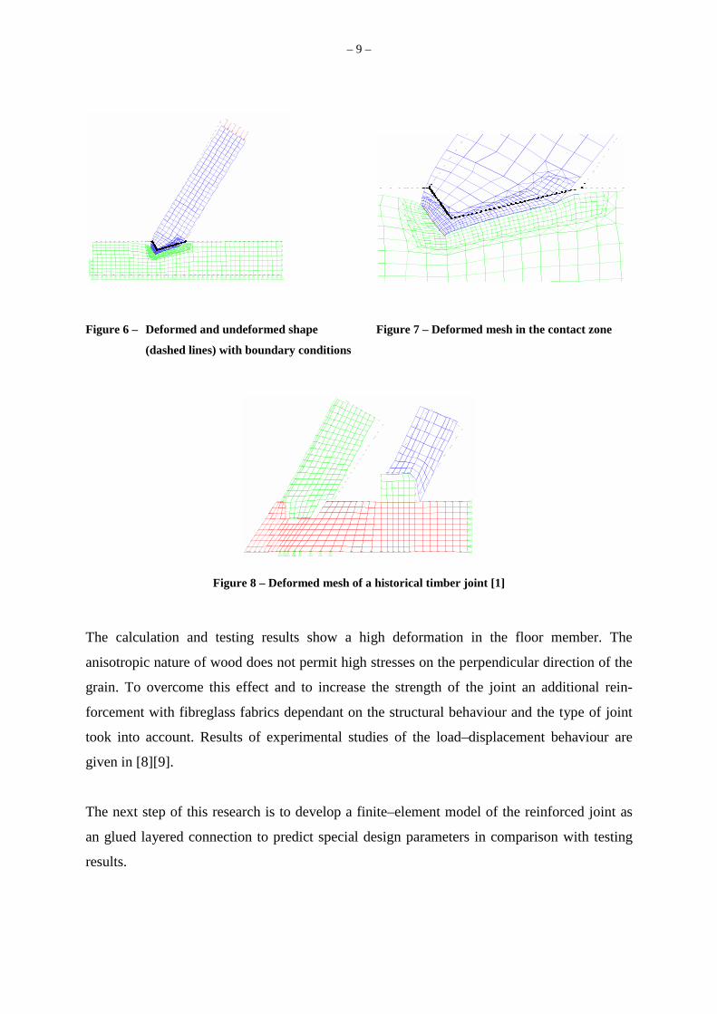
The load–displacement curves for axial loading of the rafter in direction and perpendicular of

the grain show a insignificant non-linear behaviour. The stiffness of the joints can be esti-

mated approximately by the slope of an elastic curve.

– 9 –

Figure 6 – Deformed and undeformed shape Figure 7 – Deformed mesh in the contact zone

(dashed lines) with boundary conditions

Figure 8 – Deformed mesh of a historical timber joint [1]

The calculation and testing results show a high deformation in the floor member. The

anisotropic nature of wood does not permit high stresses on the perpendicular direction of the

grain. To overcome this effect and to increase the strength of the joint an additional rein-

forcement with fibreglass fabrics dependant on the structural behaviour and the type of joint

took into account. Results of experimental studies of the load–displacement behaviour are

given in [8][9].

The next step of this research is to develop a finite–element model of the reinforced joint as

an glued layered connection to predict special design parameters in comparison with testing

results.

– 10 –

Figure 9 – Load–displacement behaviour in the rafter (in grain direction)

Figure 10 – Load–displacement behaviour perpendicular to the grain

– 11 –

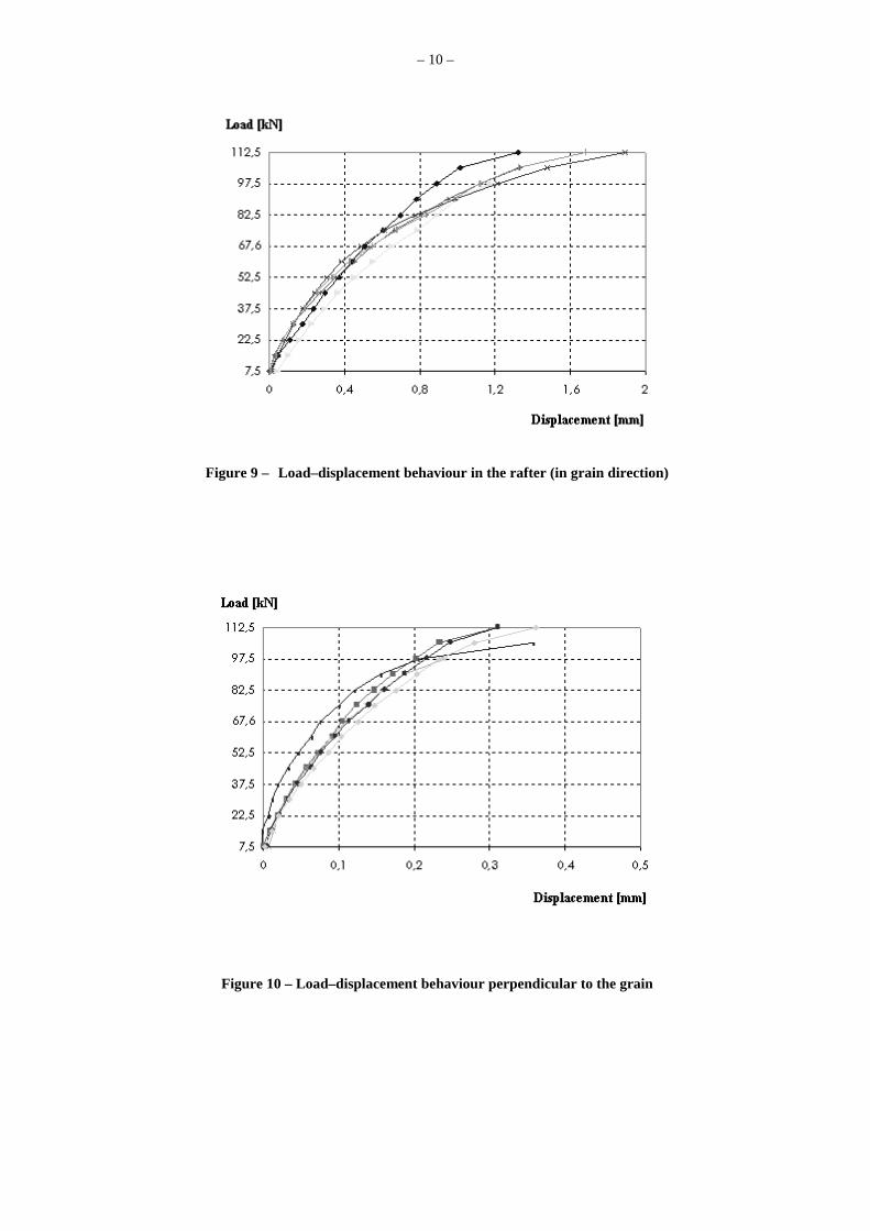
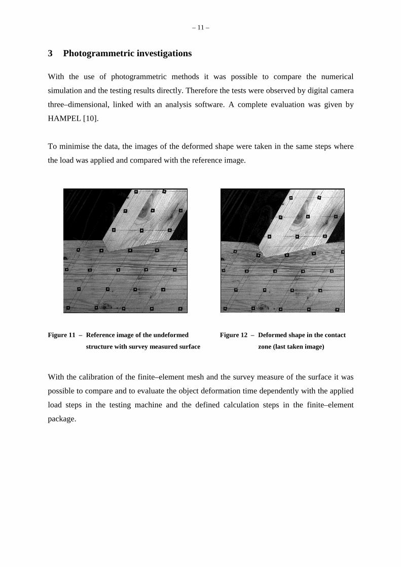
3 Photogrammetric investigations

With the use of photogrammetric methods it was possible to compare the numerical

simulation and the testing results directly. Therefore the tests were observed by digital camera

three–dimensional, linked with an analysis software. A complete evaluation was given by

HAMPEL [10].

To minimise the data, the images of the deformed shape were taken in the same steps where

the load was applied and compared with the reference image.

Figure 11 – Reference image of the undeformed Figure 12 – Deformed shape in the contact

structure with survey measured surface zone (last taken image)

With the calibration of the finite–element mesh and the survey measure of the surface it was

possible to compare and to evaluate the object deformation time dependently with the applied

load steps in the testing machine and the defined calculation steps in the finite–element

package.

– 12 –

Figure 13 – 2–D filled contour plot of horizontal Figure 14 – 2–D filled contour plot of

objectdeformation vertical objectdeformation

4 Conclusions

The step–by–step solution described is a good way to get accurate results for initially uncon-

nected bodies in an appropriate calculation time. When modelling non-linear contact between

the rafter and the floor member it is more convenient to use lower–order elements and very

important to determine the correct contact stiffness.

The stiffness of the joints can be estimated approximately by the slope of an elastic curve. To

improve the strength perpendicular to the grain and to increase the load carrying capacity of

traditional timber joints for reconstruction and redesign as well as for the development of high

performance joints, fibreglass fabrics reinforcement is an practical and low cost technique.

For that reason it’s worthwhile to determine the local stiffness of the glued layered system

with the finite–element method and laboratory tests to overcome the anisotropic properties of

timber.

– 13 –

5 References

[1] SCHOBER, K. U., „Investigation of historical timber structures in view of the three–

dimensional structure and the joints“, Diploma Thesis, Dresden University of

Technology, Dresden, 1994

[2] BODIG, J. and JAYN, B., „Mechanics of wood and wood composites“, van Nostrand

Reinhold comp., New York, 1982

[3] FAHERTY, K. and WILLIAMSON, T., „Wood engineering and construction

handbook“, 2nd edition, McGraw-Hill, New York, 1995

[4] Canadian Wood Council, „Wood Reference Handbook“, Canadian Wood Council,

Ottawa, 1991

[5] ANSYS, Inc., „ANSYS Documentation Set Rev. 5.3“, Canonsburg, PA, 1997

[6] SCHOBER, K.-U.: „Experimental and numerical investigations of traditional and

modern Timber Joints”, Numerical Simulation Working Group Document COST

C1/WD6/97-06, Coimbra (P) 1997

[7] SCHOBER, K.-U.: „Numerical Studies of Timber Joints“, EUR 18854 – COST C1 –

Control of the semi-rigid behaviour of civil engineering structural connections,

Proceedings of the international Conference Liège (B), pp. 507-516, Luxembourg 1999,

ISBN 92-828-6337-9

[8] CHEN, C. J. and HALLER, P., „Experimental Study on Fibreglass Reinforced Timber

Joints“, COST C1 Proceedings of the Second State of the Art Workshop, Prague, 1994

[9] CHEN, C. J., „The mechanical behaviour of wood reinforced by fibreglass“, Research

report, Dep. Of Civil Engineering – IBOIS, Swiss Federal Institute of Technology,

Lausanne, 1992

[10] HAMPEL, U., Photogrammetric investigations, Dresden Technical University, Dresden,

1998