Numerical Modeling of Wheat Irrigation using Coupled ...

648 SSSAJ: Volume 76: Number 2 • March–April 2012

Soil Sci. Soc. Am. J. 76:648–662Posted online 21 Dec. 2011doi:10.2136/sssaj 2010.0467Received 29 Dec. 2010*Corresponding author ([email protected]) © Soil Science Society of America, 5585 Guilford Rd., Madison WI 53711 USAAll rights reserved. No part of this periodical may be reproduced or transmitted in any form or by any means, electronic or mechanical, including photocopying, recording, or any information storage and retrieval system, without permission in writing from the publisher. Permission for printing and for reprinting the material contained herein has been obtained by the publisher.

Numerical Modeling of Wheat Irrigation using Coupled HYDRUS and WOFOST Models

Soil & Water Management & Conservation

In semiarid and arid regions, there is increasing competition for water resources between agricultural irrigation and other ecological water uses due to a grow-ing population (Molden, 1997; Seckler et al., 1998). Effi cient management

of water resources in agriculture is needed to balance water supply and demand (Tuong and Bhuiyan, 1999; Ines et al., 2002). In the last 20 yr, irrigation planning methods have switched from the allocation approach, e.g., based on socio-polit-ical considerations, to quantitative management (Paudyal and Das Gupta, 1990; Raman et al., 1992). Th e development of mathematical models is a fundamental step to guide quantitative irrigation. Th e accurate estimation of temporal and spa-tial variations in soil moisture, evaporation, and transpiration is crucial to deter-mine the availability of water resources (Aggarwal, 1995; Addiscott et al.,1995; Scanlon et al., 2002) and sustainable management of limited water resources in arid and semiarid regions (e.g., Garatuza-Payan et al., 1998).

Simulation models of crop physiological growth are widely accepted tools for fi eld study of effi cient and sustainable water use in agricultural production in various

Jian ZhouGuodong ChengXin Li

Cold and Arid Regions Environmental and Engineering Research InstituteChinese Academy of SciencesLanzhou 730000, China

Bill X. Hu*China Univ. of GeosciencesBeijing 100083, China

and

Dep. of Geological SciencesFlorida State Univ.Tallahassee, FL 32306

Genxu WangInstitute of Mountain Hazards and EnvironmentChinese Academy of SciencesChengdu 610041, China

To effi ciently manage water resources in agriculture, the hydrologic model HYDRUS-1D and the crop growth model WOFOST were coupled to improve crop production prediction through accurate simulations of actual transpi-ration with a root water uptake method and soil moisture profi le with the Richards equation during crop growth. An inverse modeling method, the shuffl ed complex evolution algorithm, was used to identify soil hydraulic parameters for simulating the soil moisture profi le. The coupled model was vali-dated by experimental study on irrigated wheat (Triticum aestivum L.) in the middle reaches of the Heihe River, northwest China, in a semiarid and arid region. Good agreement was achieved between the simulated actual evapo-transpiration, soil moisture, and crop production and their respective fi eld measurements under a realistic irrigation scheme. A water stress factor, actual root uptake with potential transpiration, is proposed as an indicator to guide irrigation. Numerical results indicated that the irrigation scheme guided by the water stress factor can save 27% of irrigation water compared with the current irrigation scheme. Based on the calibrated model, uncertainty and sensitivity analysis methods were used to predict the risk of wheat production loss with decreasing irrigation and to study the effects of coupled model parameters and environmental factors on wheat production. The analysis revealed that the most suitable groundwater depth for wheat growth is 1.5 m. These results indicate that the coupled model can be used for analysis of schemes for saving water and study of the interaction between crop growth and the hydrologic cycle.

Abbreviations: LAI, leaf area index; NSE, Nash–Sutcliffe coeffi cient; SCE, shuffl ed complex evolution; WOFOST, World Food Studies.

SSSAJ: Volume 76: Number 2 • March–April 2012 649

agro-ecological zones. Such models can aid in understanding the interactions between crops and environments (Kropff and Goudriaan, 1994; Yin et al., 2004) and provide optimal agricul-tural management strategies under uncertain weather conditions and climatic change (Meinke et al., 2001; Booltink et al., 2001; Munch et al., 2001; Kersebaum et al., 2002). Several crop physi-ological growth models (e.g., Simple and Universal Crop Growth Simulator [SUCROS] and ORYZA [Goudriaan and van Laar, 1994]; World Food Studies [WOFOST; Boogaard et al., 1998]; Genotype by Environment Interaction on Crop Growth Simulator [GECROS; Yin and van Laar 2005]; Decision Support System for Agrotechnology Transfer [DSSAT; Jones et al., 2003]) have been developed from photosynthesis modeling based on the complex biochemical approach (Farquhar et al., 1980), the constant light-use effi ciency approach, or the C assimilation approach (Arora and Boer, 2005). In crop growth modeling schemes, the various components of the water balance in an agro-ecological system are the most important physical and physiological factors for calcula-tions (Aggarwal, 1995; Addiscott et al., 1995). Spatial and tem-poral variation of soil moisture is one of the main causes of crop production variation (Shepherd et al., 2002; Anwar et al., 2003; Patil and Sheelavantar, 2004). Meanwhile, actual evaporation and transpiration, which determine the soil moisture profi le, are the main processes for water loss in a soil–plant system (Burman and Pochop, 1994; Monteith and Unsworth, 1990). Crops can only absorb the soil moisture present within reach of their roots. Th ese processes could be represented in hydrologic models. Th erefore, the coupling of hydrologic and crop growth models connects hy-drology and agronomy quantitatively and provides a bridge across the boundaries of the two subjects.

In the last several years, numerous studies have been conducted to understand the complex interactions between ecological systems and the hydrologic cycle, resulting in the development of ecohy-drologic models and soil–plant–atmosphere models (Smettem, 2008). Simulation modeling can be used to understand the re-lationships among crop production, groundwater recharge, soil evaporation, and crop transpiration (de Willigen, 1991; Engel and Priesack, 1993; Diekkrüger et al., 1995; Smith et al., 1997; Shaff er et al., 2001; van Ittersum and Donatelli, 2003). Kendy et al. (2003) used a numerical model to evaluate groundwater recharge in an ir-rigated cropland. By coupling hydrologic and crop growth models, Eitzinger et al. (2004) studied soil water movement during crop growth stages and concluded that the coupled modeling approach was better than a single-model method. A few studies have been conducted to investigate the eff ects of the soil moisture distribution along a vertical soil profi le during crop transpiration (e.g., Varado et al., 2006). Th e model coupling studies have generally focused on the eff ect of crop growth on soil moisture, and much less attention has been paid to improving crop growth models by properly modeling the root growth algorithm and root water uptake.

In this study, we developed a modeling approach to simultane-ously estimate crop production, soil moisture dynamics, evaporation, and transpiration by coupling HYDRUS with WOFOST. Th e soil moisture dynamic movements are simulated through the Richards

equation (in the HYDRUS model), while root water uptake and transpiration are calculated according to the method of Feddes et al. (1978, p. 9–30). Th e parameters of soil hydraulic properties are identi-fi ed with the shuffl ed complex evolution (SCE) algorithm. Th e CO2 assimilation (photosynthesis) and respiration of the crop are simu-lated by the WOFOST model. Th e ratio of the crop actual transpira-tion and potential transpiration is used to represent the infl uence of soil water stress on crop production. Based on the coupled model, we conducted sensitivity and uncertainty analyses to verify the coupled model approach. Th en, the coupled model was used to optimize water use for farmland irrigation and predict crop production variability due to variations in uncertain parameters and driving variables.

FIELD EXPERIMENT AND NUMERICAL MODELINGStudy Region and Experimental Station Description

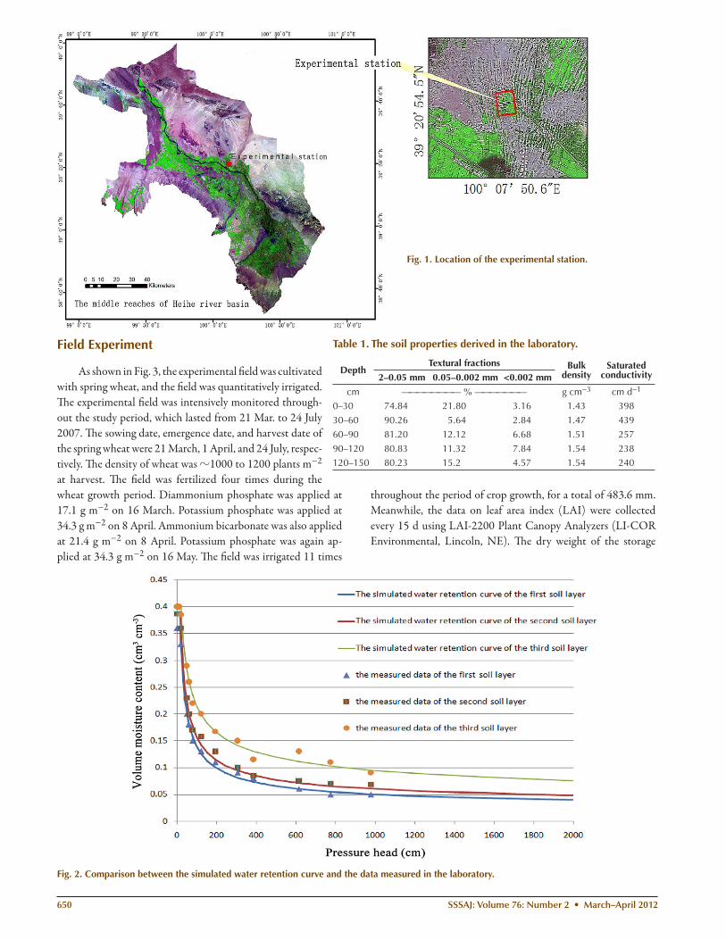
Th e Heihe River basin, located in a semiarid and arid region, is the second largest inland river basin in China. Th e region has a typical continental climate, with the mean annual precipitation and evaporation ranging from 60 to 280 and 1000 to 2000 mm, respectively. In this region, the main crops are wheat and maize (Zea mays L.), and irrigation water use effi ciency is low. Th e key to solving water scarcity and ecological problems is through ef-fective management of water resources and optimization of irri-gation. An agricultural experimental station, located at 39°20.9′ N, 100°7.8′ E, altitude 1382 m, was established in the middle reach of the Heihe River, in the northwest of China (Fig. 1). Th e experimental station is operated by the Chinese Academy of Science to study the impact of quantitative irrigation on wheat growth. Th e station is managed according to agricultural prac-tices in the Heihe River basin region, including crop rotations (spring wheat and maize) and fl ood irrigation.

Characterization of Soil PropertiesTh e experimental station was established on a sandy soil

(USDA classifi cation system). To characterize the soil physical properties, fi ve soil samples were extracted from the ground sur-face to a depth of 1.5 m at 30-cm intervals. Th e samples were analyzed in the laboratory to determine the soil bulk density (Grossman and Reinsch, 2002), water retention properties (soil water contents at 0–1000-kPa matric potentials; Equi-pf, Streat Instruments, Christchurch, New Zealand) and the percentages of sand, silt, and clay (Gee and Or, 2002). Saturated conductiv-ity was measured from the ground surface to a depth of 1.5 m at 30-cm intervals in the fi eld (2800K1 Guelph permeameter, Soilmoisture Equipment Corp., Santa Barbara, CA). Th e analy-sis results are shown in Table 1 and Fig. 2. Th e soil nutrient status was analyzed in the laboratory (TPY-6PC Soil Nutrient Tester, Zhejiang Top Instrument Co., Hangzhou, China). Th e total N, total P, available N, available K, and available P contents of the surface soil (0–30 cm) were 0.74, 1.03, 0.028, 0.126, and 0.03 g kg−1, respectively.


Field Experiment

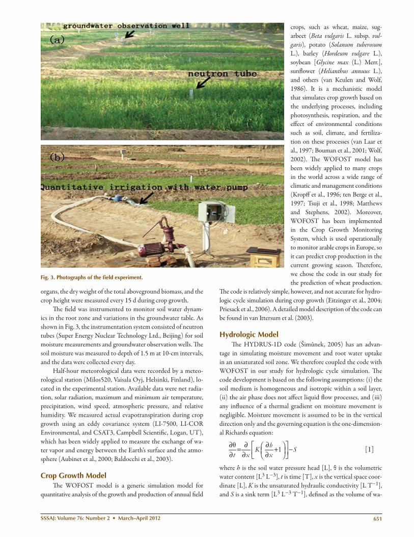
As shown in Fig. 3, the experimental fi eld was cultivated with spring wheat, and the fi eld was quantitatively irrigated. Th e experimental fi eld was intensively monitored through-out the study period, which lasted from 21 Mar. to 24 July 2007. Th e sowing date, emergence date, and harvest date of the spring wheat were 21 March, 1 April, and 24 July, respec-tively. Th e density of wheat was ?1000 to 1200 plants m−2 at harvest. Th e fi eld was fertilized four times during the wheat growth period. Diammonium phosphate was applied at 17.1 g m−2 on 16 March. Potassium phosphate was applied at 34.3 g m−2 on 8 April. Ammonium bicarbonate was also applied at 21.4 g m−2 on 8 April. Potassium phosphate was again ap-plied at 34.3 g m−2 on 16 May. Th e fi eld was irrigated 11 times

throughout the period of crop growth, for a total of 483.6 mm. Meanwhile, the data on leaf area index (LAI) were collected every 15 d using LAI-2200 Plant Canopy Analyzers (LI-COR Environmental, Lincoln, NE). Th e dry weight of the storage

Fig. 1. Location of the experimental station.

Table 1. The soil properties derived in the laboratory.

DepthTextural fractions Bulk

densitySaturated

conductivity2–0.05 mm 0.05–0.002 mm <0.002 mm

cm ———————— % ——————— g cm−3 cm d−1

0–30 74.84 21.80 3.16 1.43 398

30–60 90.26 5.64 2.84 1.47 439

60–90 81.20 12.12 6.68 1.51 257

90–120 80.83 11.32 7.84 1.54 238120–150 80.23 15.2 4.57 1.54 240

Fig. 2. Comparison between the simulated water retention curve and the data measured in the laboratory.


organs, the dry weight of the total aboveground biomass, and the crop height were measured every 15 d during crop growth.

Th e fi eld was instrumented to monitor soil water dynam-ics in the root zone and variations in the groundwater table. As shown in Fig. 3, the instrumentation system consisted of neutron tubes (Super Energy Nuclear Technology Ltd., Beijing) for soil moisture measurements and groundwater observation wells. Th e soil moisture was measured to depth of 1.5 m at 10-cm intervals, and the data were collected every day.

Half-hour meteorological data were recorded by a meteo-rological station (Milos520, Vaisala Oyj, Helsinki, Finland), lo-cated in the experimental station. Available data were net radia-tion, solar radiation, maximum and minimum air temperature, precipitation, wind speed, atmospheric pressure, and relative humidity. We measured actual evapotranspiration during crop growth using an eddy covariance system (LI-7500, LI-COR Environmental, and CSAT3, Campbell Scientifi c, Logan, UT), which has been widely applied to measure the exchange of wa-ter vapor and energy between the Earth’s surface and the atmo-sphere (Aubinet et al., 2000; Baldocchi et al., 2003).

Crop Growth ModelTh e WOFOST model is a generic simulation model for

quantitative analysis of the growth and production of annual fi eld

crops, such as wheat, maize, sug-arbeet (Beta vulgaris L. subsp. vul-garis), potato (Solanum tuberosum L.), barley (Hordeum vulgare L.), soybean [Glycine max (L.) Merr.], sunfl ower (Helianthus annuus L.), and others (van Keulen and Wolf, 1986). It is a mechanistic model that simulates crop growth based on the underlying processes, including photosynthesis, respiration, and the eff ect of environmental conditions such as soil, climate, and fertiliza-tion on these processes (van Laar et al., 1997; Bouman et al., 2001; Wolf, 2002). Th e WOFOST model has been widely applied to many crops in the world across a wide range of climatic and management conditions (Kropff et al., 1996; ten Berge et al., 1997; Tsuji et al., 1998; Matthews and Stephens, 2002). Moreover, WOFOST has been implemented in the Crop Growth Monitoring System, which is used operationally to monitor arable crops in Europe, so it can predict crop production in the current growing season. Th erefore, we chose the code in our study for the prediction of wheat production.

Th e code is relatively simple, however, and not accurate for hydro-logic cycle simulation during crop growth (Eitzinger et al., 2004; Priesack et al., 2006). A detailed model description of the code can be found in van Ittersum et al. (2003).

Hydrologic ModelTh e HYDRUS-1D code (Šimůnek, 2005) has an advan-

tage in simulating moisture movement and root water uptake in an unsaturated soil zone. We therefore coupled the code with WOFOST in our study for hydrologic cycle simulation. Th e code development is based on the following assumptions: (i) the soil medium is homogeneous and isotropic within a soil layer, (ii) the air phase does not aff ect liquid fl ow processes, and (iii) any infl uence of a thermal gradient on moisture movement is negligible. Moisture movement is assumed to be in the vertical direction only and the governing equation is the one-dimension-al Richards equation:

1hK St x xθ∂ ∂ ∂⎡ ⎤⎛ ⎞= + −⎜ ⎟⎢ ⎥∂ ∂ ∂⎝ ⎠⎣ ⎦

[1]

where h is the soil water pressure head [L], θ is the volumetric water content [L3 L−3], t is time [T], x is the vertical space coor-dinate [L], K is the unsaturated hydraulic conductivity [L T−1], and S is a sink term [L3 L−3 T−1], defi ned as the volume of wa-

Fig. 3. Photographs of the fi eld experiment.


ter removed from a unit volume of soil per unit time due to plant water uptake. Th e sink term is specifi ed in terms of a potential water uptake rate and a stress factor (Feddes et al., 1978, p. 9–30):

( ) ( )( ) ( )r p

0d

l

h R zS T

h R z z

α

α=

∫ [2]

where S is the root water uptake rate [L3 L−3 T−1], R(z) is the distribu-tion function of the root, lr is the root depth [L], Tp is the potential transpi-ration [L], and α(h) is the dimen-sionless water stress response func-tion (0 ≤ α(h) ≤ 1), which describes the reduction in uptake that occurs due to drought stress. For α(h), we used the functional form introduced by Feddes et al. (1978, p. 9–30):

( )

( ) ( )

( ) ( )

4 3 4 4 3

3 2

1 2 1 2 1

4 1

1

0 ,

h h h h h h hh h h

hh h h h h h h

h h h h

α

− − < ≤⎧⎪ < ≤⎪=⎨

− − ≤ <⎪⎪ ≤ >⎩

[3]

where h1, h2, h3, and h4 are threshold parameters. Th e uptake is at the potential rate when the pressure head is between h2 and h3. It decreases linearly when h > h2 or h < h3. Th e uptake rate becomes zero when h < h4 or h > h1. Crop-specifi c values for these parameters were chosen from the database in HYDRUS-1D (Šimůnek, 2005).

An atmospheric boundary condition was implemented at the soil surface. Th e atmospheric boundary condition required daily irrigation, precipitation rate, potential evaporation, and transpiration rate as inputs. A detailed description about how to calculate the potential evaporation and transpiration can be found in HYDRUS-1D (Šimůnek, 2005). A deep drainage con-dition was used at the bottom. Th e condition required the initial reference groundwater depth to be given (Šimůnek, 2005).

Th e soil hydraulic properties were modeled using the van Genuchten–Mualem constitutive relationships (Mualem, 1976; van Genuchten, 1980):

( ) ( )s r

r 1 1/

c

s

01

0

nnh

hh

h

θ θθ

αθ

θ

−+⎧ + <⎪ ⎡ ⎤+=⎨ ⎣ ⎦

⎪≥⎩

[4]

( ) { }21 1//( 1)s e e1 1

nl n nK h K S S−−⎡ ⎤= − −⎣ ⎦ [5]

( ) re

s r

hS

θ θθ θ

−=

− [6]

where Se is the eff ective saturation [L3 L−3], θs is the saturated water content [L3 L−3], θr is the residual water content [L3 L−3], Ks is the saturated hydraulic conductivity [L T−1], α is an air-entry parameter, n is a pore size distribution parameter, and l is a pore connectivity parameter. Th e parameters α, n, and l are empirical coeffi cients that determine the shape of the hydraulic functions. To reduce the number of free parameters, we took l = 1, a common assumption based on Mualem (1976).

We estimated the parameters in the van Genuchten–Mualem constitutive relationships using the SCE algorithm (Duan et al., 1993). Th e Nash–Sutcliff e coeffi cient (NSE) was chosen as the objective function:

( )( )

2

sim, obs,12

obs,1

NSE 1N

t ttN

tt

X X

X X=

=

−= −

−

∑∑

[7]

where N is the number of samples, X is the mean of the observed values, and Xobs,t and Xsim,t are the observed and simulated val-ues at time t, respectively.

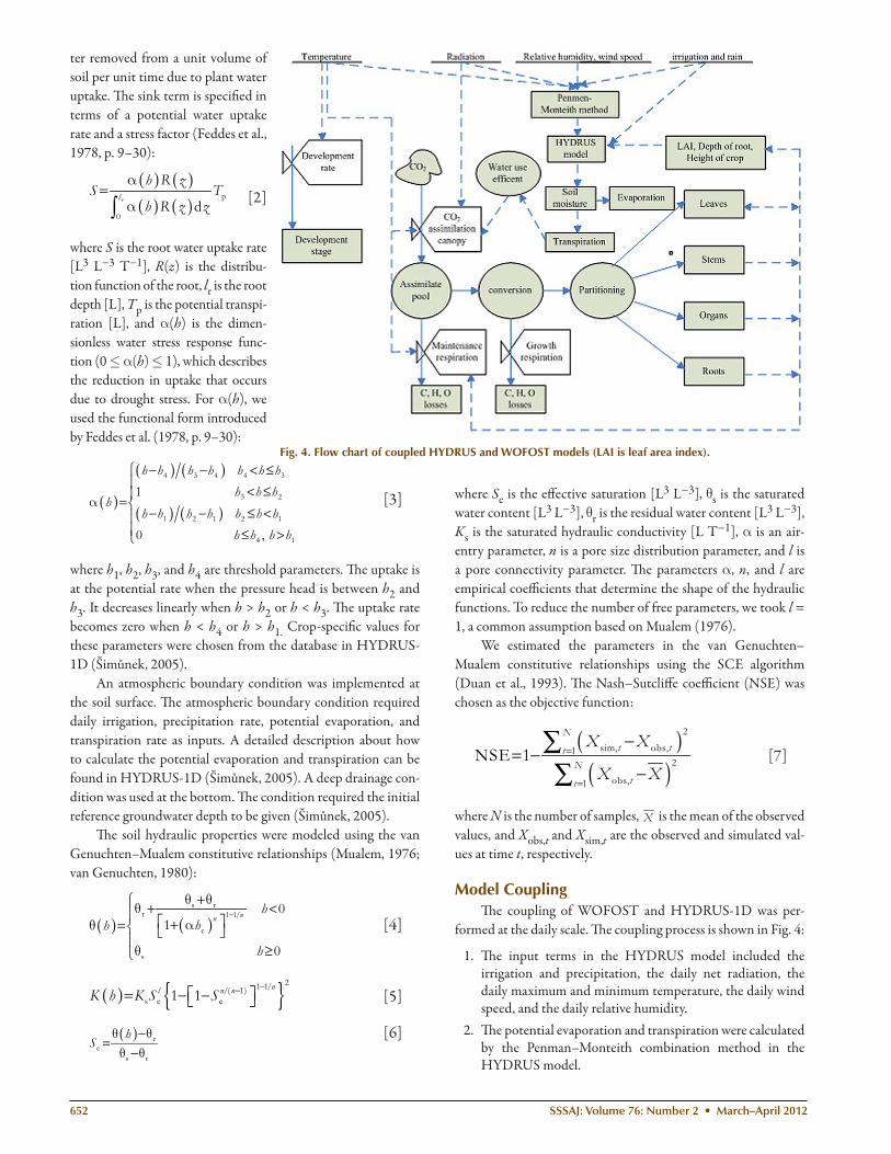
Model CouplingTh e coupling of WOFOST and HYDRUS-1D was per-

formed at the daily scale. Th e coupling process is shown in Fig. 4:

1. Th e input terms in the HYDRUS model included the irrigation and precipitation, the daily net radiation, the daily maximum and minimum temperature, the daily wind speed, and the daily relative humidity.

2. Th e potential evaporation and transpiration were calculated by the Penman–Monteith combination method in the HYDRUS model.

Fig. 4. Flow chart of coupled HYDRUS and WOFOST models (LAI is leaf area index).


3. Th e water uptake was calculated according to Feddes’ equation in the HYDRUS model.

4. Th e soil water balance, soil moisture, and groundwater depth were calculated using the HYDRUS model.

5. Th e root water uptake and actual transpiration on a daily basis were assumed to be the same because most of the root water uptake is consumed by crop transpiration. Th erefore, the ratio between the calculated actual water uptake based on the Feddes equation and the potential transpiration based on the Penman–Monteith method was regarded as an indicator of the degree of water stress.

6. Th e total potential daily gross CO2 assimilation of the crop, which was calculated according to the WOFOST model, was multiplied by the water stress ratio to calculate the actual daily CO2 assimilation. Carbohydrate allocation among various crop parts was then calculated according to the WOFOST model.

7. Th e calculated vegetation parameters from the WOFOST model, more specifi cally the rooting depth, height of the crop, and LAI, were then used as inputs for the HYDRUS model at the next step.

Sensitivity AnalysisSensitivity analysis has oft en been used to determine the

contribution of an uncertain input factor to the uncertainty in the output of interest. Sensitivity analysis was evaluated using a two-step method: the screening method proposed by Morris (1991) and a variance-based technique proposed by Soboľ (1993). Th e Morris method provides a qualitative assessment of the importance of each input factor, while the Soboľ method performs a quantitative analysis of sensitivity and uncertainty. Th is two-step methodology was used in recent studies of in-put–output relationship and model evaluation (Fox et al., 2010; Jawitz et al., 2008; Muñoz-Carpena et al., 2010).

Th e Morris method (Morris, 1991) is particularly eff ective for screening a subset of relevant parameters among those contained in models with a large number of parameters or with time-con-suming simulations. Th is one-parameter-at-a-time (OAT) method uses randomized sampling matrices that allow direct observation of each elementary eff ect on the calculation result. Assuming (i) X = (x1, ..., xk) as the k-dimensional vector of model parameters, (ii) all variables are rescaled in the 0 to 1 range, (iii) xi can take only P (the number of levels, using the Morris terminology) discrete val-ues in the set {0, 1/(P − 1),1/(P − 2), ..., 1}, and (iv) Δ is a multiple of 1/(P − 1), an elementary eff ect, EEi, is calculated as

( )

( )

1 2 1 1

1 2

, , ..., , , , ...,EE

, , ...,

i i i ki

k

y x x x x x x

y x x x

ΔΔ

Δ

− ++=

−

[8]

where y(X) is the output.Th e method calculates the distribution of the EEi for each

parameter through samples from the hyperspace Ω (identifi ed by a k-dimensional P-level grid), and then calculates the mean,

μ [the strength; assessing the overall infl uence of the param-eter on y(X)], and standard deviation, σ (the spread; estimat-ing the totality of the higher order eff ects, i.e., nonlinearity or interactions with other parameters), of the distribution of the EEi. Because the model output can be non-monotonic, Campolongo et al. (2007) suggested considering the distri-bution of the absolute values of the elementary eff ects, μ*, to avoid cancellation of eff ects with opposing signs. A large value of μ* indicates a parameter with an important overall infl uence (total eff ect), while a large value of σ indicates the parameter’s obvious interactions with other parameters. More detail on this method can be found in Saltelli et al. (2004).

Th e Soboľ approach (Soboľ, 1993) is a variance-based meth-od. its advantage over the OAT method is that it allows simulta-neous computation of the fi rst-order sensitivity index (Sx) and total-order sensitivity index (STx) for a given parameter.

Th e input parameter space Xk is assumed to be the k-dimen-sional unit hypercube:

( )1 2|0 1, 0 1, ..., 0 1kkX x x xΩ = ≤ ≤ ≤ ≤ ≤ ≤ [9]

According to Soboľ (1993), the model function f(x1, x2, ..., xk) can always be decomposed into summands of increas-ing dimension:

( ) ( )

( )( )

1 0 1 11

1

1,2,..., 1 2

, ...,

,

... , , ...,

k

ki

ij i ji j k

k k

f x x f f x

f x x

f x x x

=

≤ ≤ ≤

= +

+

+ +

∑∑

[10]

Th e total variance D of f(X) can be written as

( )2 20k

D f x fΩ

= −∫ [11]

while each partial variance, corresponding to a generic term fi1...is can be written as

( )1 1 1 1

1 1 2... ...0 0

1

, ..., d ...d

1 ...and

1, 2, ...

s s s si i i i i i i i

s

D f x x x x

i i k

s k

=

≤ < < ≤

=

∫ ∫ [12]

All the quantities, f0, D, Di1…is, can be computed by multidimen-sional Monte Carlo integration (e.g., Press and Farrar, 1990).

Sensitivity estimates are then defi ned as

1

1

......

s

s

i ii i

DS

D= [13]

where Si represents the fi rst-order sensitivity and Sij are second-order sensitivities. Th e higher order terms are represented by this analogy.

Total sensitivity indices (STi) are then defi ned as


T 1,2,..., ,...,1

...k

i i ij i kj

S S S S=

= + + +∑ [14]

In our study, the weight of storage organs (WSO), representing physiological maturity, was selected as the sensitivity analysis model output variable because it is a synthetic representation of the numerical model’s results. Th e variation of WSO in re-sponse to variations in the crop and environment parameters were investigated using the Morris and Soboľ sensitivity meth-ods, conducted by SimLab Dynamic Link Library (simlab.jrc.ec.europa.eu/; verifi ed 20 Nov. 2011), integrated with the coupled HYDRUS and WOFOST models.

Before performing the sensitivity analysis, the ranges of the 34 input factors were determined (Table 2) based on values from literature review, experience, research objectives, and the default minimum and maximum values in the WOFOST and HYDRUS databases. Uniform distributions were assigned to input factors when only the base values were known, the ranges were consid-ered fi nite, and no explicit knowledge of the distributions was available (McKay, 1995). Th is conservative assumption allowed an equal probability of occurrence of the input factors along the probability range (Muñoz-Carpena et al., 2010). We divided the parameters into 13 groups according to their physical properties and functions.

Table 2. Parameter groups and the ranges of parameters used in the coupled model.

Group Parameter Defi nition Range

1. Sowing date IDSOW sowing date 83–97 d2. Groundwater depth ZIT initial depth of groundwater table 50–500 cm

3. Soil hydraulic parameters (HYDRUS)

HYDRUS model parameters

soil hydraulic parameters θr, 0.01–0.1 m m−1

θs, 0.25–0.4 m m−1

a, 0.02–0.14

n, 0.2–0.6

Ks, 10–800 cm d−1

4. Emergence TSUMEM thermal time from sowing to emergence 45–55°C d−1

TBASEM lower threshold temperature for emergence −2 to 3°CTEFFMX maximum effective temperature for emergence 20–32°C

5. Phenology TSUM1 thermal time from emergence to anthesis 80–1050°C d−1

TSUM2 thermal time from anthesis to maturity 80–1200°C d−1

6. Initial RGRLAI maximum relative increase in leaf area index 0.007–0.01 ha ha−1 d−1

LAIEM leaf area index at emergence 0.1–0.2 ha ha−1

7. Green area SPAN life span of leaves growing at 35°C 26–36 d

SLATB specifi c leaf area as a function of development stage 0.001–0.003 ha kg−1

8. Assimilation AMAXTB maximum leaf CO2 assimilation rate at development stage of crop growth

28–43 kg ha−1 h−1

AMAXTB1 maximum leaf CO2 assimilation rate at development stage of crop maturity

2–8 kg ha−1 h−1

EFFTB initial light-use effi ciency of assimilation of leave as function of daily temperature

0.4–0.5 kg ha−1 h−1 (J m−2 s−1) °C

KDIFTB extinction coeffi cient for diffuse visible light as function of development stage

0.5–0.7

9. Conversion of assimilates into biomass

CVO conversion effi ciency of assimilates into storage organ 0.6–0.8 kg kg−1

CVS conversion effi ciency of assimilates into stem 0.59–0.76 kg kg−1

CVL conversion effi ciency of assimilates into leaf 0.61–0.75 kg kg−1

CVR conversion effi ciency of assimilates into root 0.62–0.76 kg kg−1

10. Maintenance respiration

RMS relative maintenance respiration rate stems 0.013–0.02 kg CH2O kg−1 d−1

RML relative maintenance respiration rate leaves 0.027–0.033 kg CH2O kg−1 d−1

Q10 relative change in respiration rate per 10°C temperature change

1.6–2

RMO relative maintenance respiration rate storage organs 0.005–0.015 kg CH2O kg−1 d−1

RMR relative maintenance respiration rate roots 0.01–0.016 kg CH2O kg−1 d−1

11. Death rates due to water stress

PERDL maximum relative death rate of leaves due to water stress

0.02–0.06 kg kg−1 d−1

12. Correction factor transpiration rate

CFET correction factor transpiration rate 0.7–1.2

13. Root parameters RRI maximum daily increase in rooting depth 1–2 cm d−1

RDI initial rooting depth 7–14 cmRDMCR maximum rooting depth 80.5–120 cm


For the Morris method, the means and standard deviations of the sensitivity parameters (μ* and σ) were obtained from analyses using the total range of trajectories (10) and levels (four) (Saltelli et al., 2004). Sensitivity analysis experiments required 320 simula-tions for each input factor. For the Soboľ method, Monte Carlo sample size was set to 5000 for each input factor.

RESULTS AND DISCUSSIONModel Validation

Th is study focused on the impact of water shortage on wheat growth in the study region. Because the fi eld was fertilized four times during wheat growth, plant nutrients were assumed to be not limiting for numerical simulation.

Running the coupled model required various inputs, such as daily weather data (minimum temperature, maximum tempera-ture, irradiation, vapor pressure, wind speed, and precipitation) and irrigation schemes on a daily basis, the parameters of crop characteristics (including parameters pertaining to phenology, as-similation and respiration characteristics, and partitioning of as-similates to plant organs) and the soil hydraulic parameters (θr, θs, a, n, and Ks). Th e meteorological data were acquired from the me-teorological station. Th e amounts and durations of irrigation were recorded individually. Many characteristics of the wheat 22 culti-var in our study were similar to those of the wheat 102 cultivar in the WOFOST crop database, with respect to drought resistance, cold resistance, plant height, leaf width, grain size, and so on, so the wheat data set (wheat 102), which was provided by the European Community (Boons-Prins et al., 1993), was used in this study.

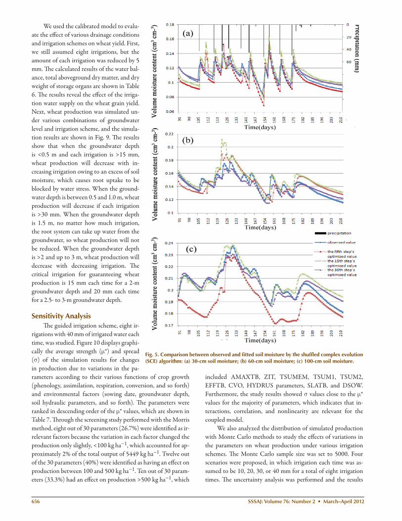
At the study site, the soil profi le is vertically divided into three layers according to the soil physical properties at the 0- to 30-, 30- to 60-, and 60- to 150-cm depths. Th e saturated conduc-tivity values of the three soil layers were measured and used as in-puts. Th e optimized soil hydraulic parameters of the layers were estimated using the SCE algorithm. Th e NSE values between the fi tted and observed data for the three layers in diff erent iterative steps are shown in Table 3. Th e fi nal optimized parameters are shown in Table 4. Th e comparison between the fi tted soil mois-ture using the SCE algorithm and the observed soil moisture is shown in Fig. 5. Th e optimized parameters, which were inversely calculated through the SCE algorithm, were used to fi t the water retention curve using the van Genuchten–Mualem relationship. Th e comparison between the fi tted water retention curve and

the measured data in laboratory is shown in Fig. 2.Th e RMSEs for the water retention curves of the three soil layers are 0.005, 0.007, and 0.05 m3 m−3, respectively.

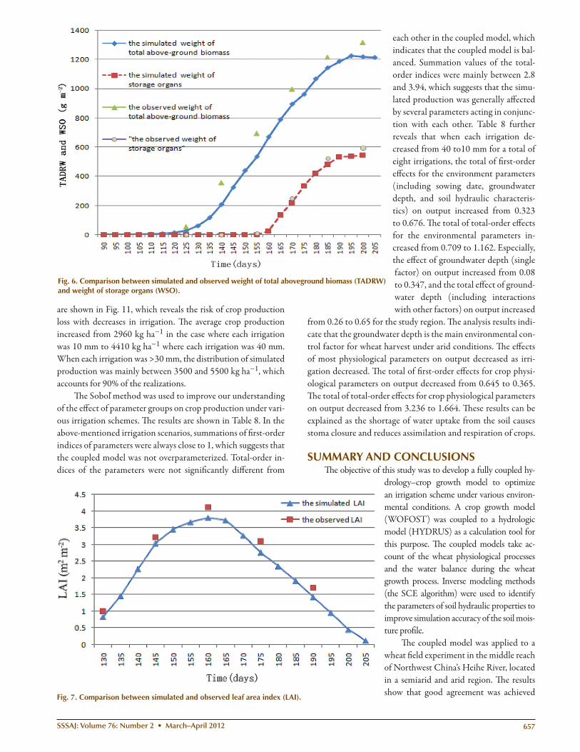
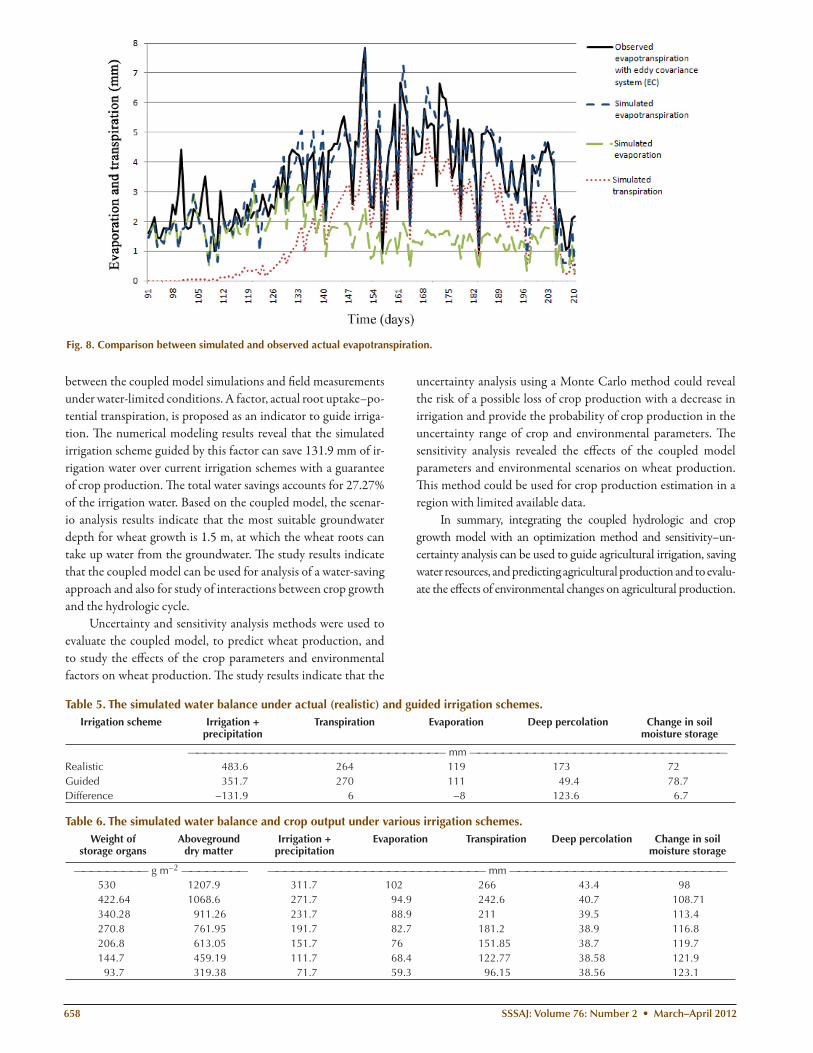
Th e simulation period was from the planting date on 21 Mar. 2007 to the harvest date on 24 July 2007. Th e computation time step was 1 d. Th e simulated results of the total aboveground dry matter, dry weight of storage organs, and LAI as well as their observed values in the fi eld are shown in Fig. 6 and 7. Th e RMSEs of the total aboveground dry matter, dry weight of storage or-gans, and LAI are 49.79 g m−2, 24.36 g m−2, and 0.26 m2 m−2, respectively, and the respective NSE values are 0.978, 0.98, and 0.948. Th e results show that the simulated dry matter accumu-lation and partitioning among the various crop organs matched the observations well. Th e comparison between simulated and observed actual evapotranspiration is shown in Fig. 8. Th e RMSE and NSE values for actual evapotranspiration are 0.705 mm and 0.798, respectively. Th e results show that the simulated evapotranspiration also matched well with the value observed by the eddy covariance systems. Th e simulated evapotranspiration was divided into actual transpiration and actual evaporation, which are shown in Fig. 8. Th e cumulative actual transpiration and evaporation were 264 and 119 mm, respectively. Th e results reveal that the crop’s eff ective transpiration was approximately 2.2 times the soil evaporation during wheat growth under the realistic irrigation scheme. Th e above calculation results indicate that the selected parameter values are reasonable for local wheat characteristics and soil properties in the study fi eld. Th e coupled model can be used to quantitatively predict agricultural produc-tion under water-limited conditions.

Th e calibrated model was then used to evaluate the water balance and to search for a potential water-saving scheme. When the ratio between actual root uptake and potential transpiration is <0.9, the wheat would be quantitatively irrigated with 40 mm of water. Th e simulated results indicated that a total of eight ir-rigations was needed, which would be on the Days of the Year 130, 140, 146, 153, 160, 166, 173, and 191. Th e simulated water balance under the guided irrigation scheme was compared with the fi eld results, which are shown in Table 5. Th ese results indi-cate that the guided irrigation scheme could save 131.9 mm of irrigation water. Th e saving in water is mainly due to decreases in deep percolation (123.6 mm), which account for 93.7% of the total water savings. Transpiration and evaporation under the guided irrigation scheme is close to that under the actual irriga-tion scheme, so crop production could be guaranteed.

Table 3. The Nash–Sutcliffe coeffi cient of the fi t to observed data for three soil layers during the algorithm iterative pro-cess. The soil moisture of the fi rst layer (0–30 cm) is repre-sented by 30-cm observed soil moisture, the soil moisture of the second layer (30–60 cm) by 60-cm observed soil moisture, and the soil moisture of the third layer (60–150 cm) by 100-cm observed soil moisture).

Iterative stepNash–Sutcliffe coeffi cient

30-cm soil moisture

60-cm soil moisture

100-cm soil moisture

After the 5th step 0.385895 0.092972 −0.567474After the 15th step 0.315185 0.136020 0.788971After the 30th step 0.750535 0.746587 0.875384

Table 4. The parameters of soil hydraulic properties, including the residual and saturated moisture content (θr and θs, respec-tively), an air-entry parameter (α), and pore size distribution parameter (n), of three layers estimated by the shuffl ed com-plex evolution algorithm.

Layer θr θs α n

———— m3 m−3 ————First 0.018 0.36 0.06 0.6

Second 0.025 0.38 0.06 0.57Third 0.021 0.4 0.05 0.42


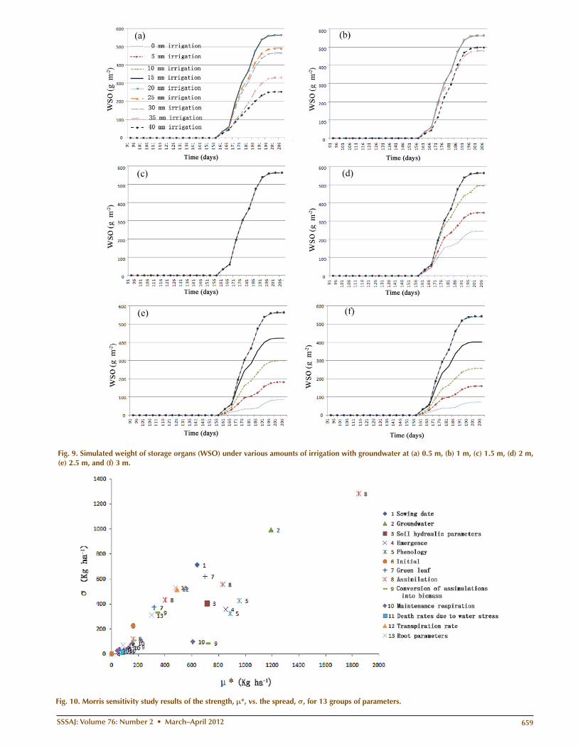
We used the calibrated model to evalu-ate the eff ect of various drainage conditions and irrigation schemes on wheat yield. First, we still assumed eight irrigations, but the amount of each irrigation was reduced by 5 mm. Th e calculated results of the water bal-ance, total aboveground dry matter, and dry weight of storage organs are shown in Table 6. Th e results reveal the eff ect of the irriga-tion water supply on the wheat grain yield. Next, wheat production was simulated un-der various combinations of groundwater level and irrigation scheme, and the simula-tion results are shown in Fig. 9. Th e results show that when the groundwater depth is <0.5 m and each irrigation is >15 mm, wheat production will decrease with in-creasing irrigation owing to an excess of soil moisture, which causes root uptake to be blocked by water stress. When the ground-water depth is between 0.5 and 1.0 m, wheat production will decrease if each irrigation is >30 mm. When the groundwater depth is 1.5 m, no matter how much irrigation, the root system can take up water from the groundwater, so wheat production will not be reduced. When the groundwater depth is >2 and up to 3 m, wheat production will decrease with decreasing irrigation. Th e critical irrigation for guaranteeing wheat production is 15 mm each time for a 2-m groundwater depth and 20 mm each time for a 2.5- to 3-m groundwater depth.

Sensitivity AnalysisTh e guided irrigation scheme, eight ir-

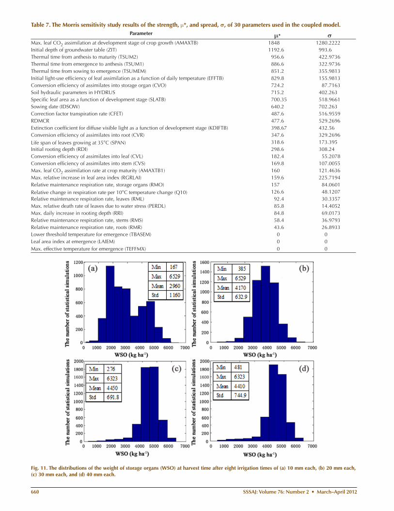
rigations with 40 mm of irrigated water each time, was studied. Figure 10 displays graphi-cally the average strength (μ*) and spread (σ) of the simulation results for changes in production due to variations in the pa-rameters according to their various functions of crop growth (phenology, assimilation, respiration, conversion, and so forth) and environmental factors (sowing date, groundwater depth, soil hydraulic parameters, and so forth). Th e parameters were ranked in descending order of the μ* values, which are shown in Table 7. Th rough the screening study performed with the Morris method, eight out of 30 parameters (26.7%) were identifi ed as ir-relevant factors because the variation in each factor changed the production only slightly, <100 kg ha−1, which accounted for ap-proximately 2% of the total output of 5449 kg ha−1. Twelve out of the 30 parameters (40%) were identifi ed as having an eff ect on production between 100 and 500 kg ha−1. Ten out of 30 param-eters (33.3%) had an eff ect on production >500 kg ha−1, which

included AMAXTB, ZIT, TSUMEM, TSUM1, TSUM2, EFFTB, CVO, HYDRUS parameters, SLATB, and DSOW. Furthermore, the study results showed σ values close to the μ* values for the majority of parameters, which indicates that in-teractions, correlation, and nonlinearity are relevant for the coupled model.

We also analyzed the distribution of simulated production with Monte Carlo methods to study the eff ects of variations in the parameters on wheat production under various irrigation schemes. Th e Monte Carlo sample size was set to 5000. Four scenarios were proposed, in which irrigation each time was as-sumed to be 10, 20, 30, or 40 mm for a total of eight irrigation times. Th e uncertainty analysis was performed and the results

Fig. 5. Comparison between observed and fi tted soil moisture by the shuffl ed complex evolution (SCE) algorithm: (a) 30-cm soil moisture; (b) 60-cm soil moisture; (c) 100-cm soil moisture.


are shown in Fig. 11, which reveals the risk of crop production loss with decreases in irrigation. Th e average crop production increased from 2960 kg ha−1 in the case where each irrigation was 10 mm to 4410 kg ha−1 where each irrigation was 40 mm. When each irrigation was >30 mm, the distribution of simulated production was mainly between 3500 and 5500 kg ha−1, which accounts for 90% of the realizations.

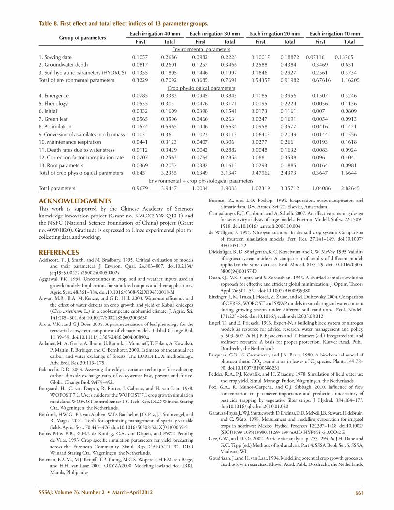
Th e Soboľ method was used to improve our understanding of the eff ect of parameter groups on crop production under vari-ous irrigation schemes. Th e results are shown in Table 8. In the above-mentioned irrigation scenarios, summations of fi rst-order indices of parameters were always close to 1, which suggests that the coupled model was not overparameterized. Total-order in-dices of the parameters were not signifi cantly diff erent from

each other in the coupled model, which indicates that the coupled model is bal-anced. Summation values of the total-order indices were mainly between 2.8 and 3.94, which suggests that the simu-lated production was generally aff ected by several parameters acting in conjunc-tion with each other. Table 8 further reveals that when each irrigation de-creased from 40 to10 mm for a total of eight irrigations, the total of fi rst-order eff ects for the environment parameters (including sowing date, groundwater depth, and soil hydraulic characteris-tics) on output increased from 0.323 to 0.676. Th e total of total-order eff ects for the environmental parameters in-creased from 0.709 to 1.162. Especially, the eff ect of groundwater depth (single factor) on output increased from 0.08 to 0.347, and the total eff ect of ground-water depth (including interactions with other factors) on output increased

from 0.26 to 0.65 for the study region. Th e analysis results indi-cate that the groundwater depth is the main environmental con-trol factor for wheat harvest under arid conditions. Th e eff ects of most physiological parameters on output decreased as irri-gation decreased. Th e total of fi rst-order eff ects for crop physi-ological parameters on output decreased from 0.645 to 0.365. Th e total of total-order eff ects for crop physiological parameters on output decreased from 3.236 to 1.664. Th ese results can be explained as the shortage of water uptake from the soil causes stoma closure and reduces assimilation and respiration of crops.

SUMMARY AND CONCLUSIONSTh e objective of this study was to develop a fully coupled hy-

drology–crop growth model to optimize an irrigation scheme under various environ-mental conditions. A crop growth model (WOFOST) was coupled to a hydrologic model (HYDRUS) as a calculation tool for this purpose. Th e coupled models take ac-count of the wheat physiological processes and the water balance during the wheat growth process. Inverse modeling methods (the SCE algorithm) were used to identify the parameters of soil hydraulic properties to improve simulation accuracy of the soil mois-ture profi le.

Th e coupled model was applied to a wheat fi eld experiment in the middle reach of Northwest China’s Heihe River, located in a semiarid and arid region. Th e results show that good agreement was achieved

Fig. 6. Comparison between simulated and observed weight of total aboveground biomass (TADRW) and weight of storage organs (WSO).

Fig. 7. Comparison between simulated and observed leaf area index (LAI).


between the coupled model simulations and fi eld measurements under water-limited conditions. A factor, actual root uptake–po-tential transpiration, is proposed as an indicator to guide irriga-tion. Th e numerical modeling results reveal that the simulated irrigation scheme guided by this factor can save 131.9 mm of ir-rigation water over current irrigation schemes with a guarantee of crop production. Th e total water savings accounts for 27.27% of the irrigation water. Based on the coupled model, the scenar-io analysis results indicate that the most suitable groundwater depth for wheat growth is 1.5 m, at which the wheat roots can take up water from the groundwater. Th e study results indicate that the coupled model can be used for analysis of a water-saving approach and also for study of interactions between crop growth and the hydrologic cycle.

Uncertainty and sensitivity analysis methods were used to evaluate the coupled model, to predict wheat production, and to study the eff ects of the crop parameters and environmental factors on wheat production. Th e study results indicate that the

uncertainty analysis using a Monte Carlo method could reveal the risk of a possible loss of crop production with a decrease in irrigation and provide the probability of crop production in the uncertainty range of crop and environmental parameters. Th e sensitivity analysis revealed the eff ects of the coupled model parameters and environmental scenarios on wheat production. Th is method could be used for crop production estimation in a region with limited available data.

In summary, integrating the coupled hydrologic and crop growth model with an optimization method and sensitivity–un-certainty analysis can be used to guide agricultural irrigation, saving water resources, and predicting agricultural production and to evalu-ate the eff ects of environmental changes on agricultural production.

Table 5. The simulated water balance under actual (realistic) and guided irrigation schemes.Irrigation scheme Irrigation +

precipitationTranspiration Evaporation Deep percolation Change in soil

moisture storage

———————————————————————————————— mm ———————————————————————————————— Realistic 483.6 264 119 173 72Guided 351.7 270 111 49.4 78.7Difference −131.9 6 −8 123.6 6.7

Table 6. The simulated water balance and crop output under various irrigation schemes.Weight of

storage organsAboveground

dry matterIrrigation +

precipitationEvaporation Transpiration Deep percolation Change in soil

moisture storage

————————— g m−2 ———————— ——————————————————————————— mm ——————————————————————————— 530 1207.9 311.7 102 266 43.4 98422.64 1068.6 271.7 94.9 242.6 40.7 108.71340.28 911.26 231.7 88.9 211 39.5 113.4270.8 761.95 191.7 82.7 181.2 38.9 116.8206.8 613.05 151.7 76 151.85 38.7 119.7144.7 459.19 111.7 68.4 122.77 38.58 121.993.7 319.38 71.7 59.3 96.15 38.56 123.1

Fig. 8. Comparison between simulated and observed actual evapotranspiration.


Fig. 9. Simulated weight of storage organs (WSO) under various amounts of irrigation with groundwater at (a) 0.5 m, (b) 1 m, (c) 1.5 m, (d) 2 m, (e) 2.5 m, and (f) 3 m.

Fig. 10. Morris sensitivity study results of the strength, μ*, vs. the spread, σ, for 13 groups of parameters.


Table 7. The Morris sensitivity study results of the strength, μ*, and spread, σ, of 30 parameters used in the coupled model.Parameter μ* σ

Max. leaf CO2 assimilation at development stage of crop growth (AMAXTB) 1848 1280.2222Initial depth of groundwater table (ZIT) 1192.6 993.6Thermal time from anthesis to maturity (TSUM2) 956.6 422.9736Thermal time from emergence to anthesis (TSUM1) 886.6 322.9736Thermal time from sowing to emergence (TSUMEM) 851.2 355.9813Initial light-use effi ciency of leaf assimilation as a function of daily temperature (EFFTB) 829.8 155.9813Conversion effi ciency of assimilates into storage organ (CVO) 724.2 87.7163Soil hydraulic parameters in HYDRUS 715.2 402.263Specifi c leaf area as a function of development stage (SLATB) 700.35 518.9661Sowing date (IDSOW) 640.2 702.263Correction factor transpiration rate (CFET) 487.6 516.9559RDMCR 477.6 529.2696Extinction coeffi cient for diffuse visible light as a function of development stage (KDIFTB) 398.67 432.56Conversion effi ciency of assimilates into root (CVR) 347.6 329.2696Life span of leaves growing at 35°C (SPAN) 318.6 173.395Initial rooting depth (RDI) 298.6 308.24Conversion effi ciency of assimilates into leaf (CVL) 182.4 55.2078Conversion effi ciency of assimilates into stem (CVS) 169.8 107.0055Max. leaf CO2 assimilation rate at crop maturity (AMAXTB1) 160 121.4636Max. relative increase in leaf area index (RGRLAI) 159.6 225.7194Relative maintenance respiration rate, storage organs (RMO) 157 84.0601Relative change in respiration rate per 10°C temperature change (Q10) 126.6 48.1207Relative maintenance respiration rate, leaves (RML) 92.4 30.3357Max. relative death rate of leaves due to water stress (PERDL) 85.8 14.4052Max. daily increase in rooting depth (RRI) 84.8 69.0173Relative maintenance respiration rate, stems (RMS) 58.4 36.9793Relative maintenance respiration rate, roots (RMR) 43.6 26.8933Lower threshold temperature for emergence (TBASEM) 0 0Leaf area index at emergence (LAIEM) 0 0Max. effective temperature for emergence (TEFFMX) 0 0

Fig. 11. The distributions of the weight of storage organs (WSO) at harvest time after eight irrigation times of (a) 10 mm each, (b) 20 mm each, (c) 30 mm each, and (d) 40 mm each.


ACKNOWLEDGMENTSTh is work is supported by the Chinese Academy of Sciences knowledge innovation project (Grant no. KZCX2-YW-Q10-1) and the NSFC (National Science Foundation of China) project (Grant no. 40901020). Gratitude is expressed to Linze experimental plot for collecting data and working.

REFERENCESAddiscott, T., J. Smith, and N. Bradbury. 1995. Critical evaluation of models

and their parameters. J. Environ. Qual. 24:803–807. doi:10.2134/jeq1995.00472425002400050002x

Aggarwal, P.K. 1995. Uncertainties in crop, soil and weather inputs used in growth models: Implications for simulated outputs and their applications. Agric. Syst. 48:361–384. doi:10.1016/0308-521X(94)00018-M

Anwar, M.R., B.A. McKenzie, and G.D. Hill. 2003. Water-use effi ciency and the eff ect of water defi cits on crop growth and yield of Kabuli chickpea (Cicer arietinum L.) in a cool-temperate subhumid climate. J. Agric. Sci. 141:285–301. doi:10.1017/S0021859603003630

Arora, V.K., and G.J. Boer. 2005. A parameterization of leaf phenology for the terrestrial ecosystem component of climate models. Global Change Biol. 11:39–59. doi:10.1111/j.1365-2486.2004.00890.x

Aubinet, M., A. Grelle, A. Ibrom, Ü. Rannik, J. Moncrieff , T. Foken, A. Kowalski, P. Martin, P. Berbiger, and C. Bernhofer. 2000. Estimates of the annual net carbon and water exchange of forests: Th e EUROFLUX methodology. Adv. Ecol. Res. 30:113–175.

Baldocchi, D.D. 2003. Assessing the eddy covariance technique for evaluating carbon dioxide exchange rates of ecosystems: Past, present and future. Global Change Biol. 9:479–492.

Boogaard, H., C. van Diepen, R. Rötter, J. Cabrera, and H. van Laar. 1998. WOFOST 7.1: User’s guide for the WOFOST 7.1 crop growth simulation model and WOFOST control center 1.5. Tech. Rep. DLO Winand Staring Ctr., Wageningen, the Netherlands.

Booltink, H.W.G., B.J. van Alphen, W.D. Batchelor, J.O. Paz, J.J. Stoorvogel, and R. Vargas. 2001. Tools for optimizing management of spatially-variable fi elds. Agric. Syst. 70:445–476. doi:10.1016/S0308-521X(01)00055-5

Boons-Prins, E.R., G.H.J. de Koning, C.A. van Diepen, and F.W.T. Penning de Vries. 1993. Crop specifi c simulation parameters for yield forecasting across the European Community. Simul. Rep. CABO-TT 32. DLO Winand Staring Ctr., Wageningen, the Netherlands.

Bouman, B.A.M., M.J. Kropff , T.P. Tuong, M.C.S. Wopereis, H.F.M. ten Berge, and H.H. van Laar. 2001. ORYZA2000: Modeling lowland rice. IRRI, Manila, Philippines.

Burman, R., and L.O. Pochop. 1994. Evaporation, evapotranspiration and climatic data. Dev. Atmos. Sci. 22. Elsevier, Amsterdam.

Campolongo, F., J. Cariboni, and A. Saltelli. 2007. An eff ective screening design for sensitivity analysis of large models. Environ. Modell. Soft w. 22:1509–1518. doi:10.1016/j.envsoft .2006.10.004

de Willigen, P. 1991. Nitrogen turnover in the soil crop system: Comparison of fourteen simulation models. Fert. Res. 27:141–149. doi:10.1007/BF01051122

Diekkrüger, B., D. Söndgerath, K.C. Kersebaum, and C.W. McVoy. 1995. Validity of agroecosystem models: A comparison of results of diff erent models applied to the same data set. Ecol. Modell. 81:3–29. doi:10.1016/0304-3800(94)00157-D

Duan, Q., V.K. Gupta, and S. Sorooshian. 1993. A shuffl ed complex evolution approach for eff ective and effi cient global minimization. J. Optim. Th eory Appl. 76:501–521. doi:10.1007/BF00939380

Eitzinger, J., M. Trnka, J. Hösch, Z. Žalud, and M. Dubrovský. 2004. Comparison of CERES, WOFOST and SWAP models in simulating soil water content during growing season under diff erent soil conditions. Ecol. Modell. 171:223–246. doi:10.1016/j.ecolmodel.2003.08.012

Engel, T., and E. Priesack. 1993. Expert-N, a building block system of nitrogen models as resource for advice, research, water management and policy. p. 503–507. In H.J.P. Eijsackers and T. Hamers (ed.) Integrated soil and sediment research: A basis for proper protection. Kluwer Acad. Publ., Dordrecht, the Netherlands.

Farquhar, G.D., S. Caemmerer, and J.A. Berry. 1980. A biochemical model of photosynthetic CO2 assimilation in leaves of C3 species. Planta 149:78–90. doi:10.1007/BF00386231

Feddes, R.A., P.J. Kowalik, and H. Zaradny. 1978. Simulation of fi eld water use and crop yield. Simul. Monogr. Pudoc, Wageningen, the Netherlands.

Fox, G.A., R. Muñoz-Carpena, and G.J. Sabbagh. 2010. Infl uence of fl ow concentration on parameter importance and prediction uncertainty of pesticide trapping by vegetative fi lter strips. J. Hydrol. 384:164–173. doi:10.1016/j.jhydrol.2010.01.020

Garatuza-Payan, J., W.J. Shuttleworth, D. Encinas, D.D. McNeil, J.B. Stewart, H. deBruin, and C. Watts. 1998. Measurement and modelling evaporation for irrigated crops in northwest Mexico. Hydrol. Processes 12:1397–1418. doi:10.1002/(SICI)1099-1085(199807)12:9<1397::AID-HYP644>3.0.CO;2-E

Gee, G.W., and D. Or. 2002. Particle size analysis. p. 255–294. In J.H. Dane and G.C. Topp (ed.) Methods of soil analysis. Part 4. SSSA Book Ser. 5. SSSA, Madison, WI.

Goudriaan, J., and H. van Laar. 1994. Modelling potential crop growth processes: Textbook with exercises. Kluwer Acad. Publ., Dordrecht, the Netherlands.

Table 8. First effect and total effect indices of 13 parameter groups.

Group of parametersEach irrigation 40 mm Each irrigation 30 mm Each irrigation 20 mm Each irrigation 10 mm

First Total First Total First Total First Total

Environmental parameters1. Sowing date 0.1057 0.2686 0.0982 0.2228 0.10017 0.18872 0.07316 0.13765

2. Groundwater depth 0.0817 0.2601 0.1257 0.3466 0.2588 0.4384 0.3469 0.651

3. Soil hydraulic parameters (HYDRUS) 0.1355 0.1805 0.1446 0.1997 0.1846 0.2927 0.2561 0.3734

Total of environmental parameters 0.3229 0.7092 0.3685 0.7691 0.54357 0.91982 0.67616 1.16205

Crop physiological parameters

4. Emergence 0.0785 0.3383 0.0945 0.3843 0.1085 0.3956 0.1507 0.3246

5. Phenology 0.0535 0.303 0.0476 0.3171 0.0195 0.2224 0.0056 0.1136

6. Initial 0.0332 0.1609 0.0398 0.1541 0.0173 0.1161 0.007 0.0809

7. Green leaf 0.0565 0.3596 0.0466 0.263 0.0247 0.1691 0.0054 0.0913

8. Assimilation 0.1574 0.5965 0.1446 0.6634 0.0958 0.3577 0.0416 0.1421

9. Conversion of assimilates into biomass 0.103 0.36 0.1023 0.3113 0.06402 0.2049 0.0144 0.1556

10. Maintenance respiration 0.0441 0.3123 0.0407 0.306 0.0277 0.266 0.0193 0.1618

11. Death rates due to water stress 0.0112 0.3429 0.0042 0.2882 0.0048 0.1632 0.0083 0.0924

12. Correction factor transpiration rate 0.0707 0.2563 0.0764 0.2858 0.088 0.3538 0.096 0.404

13. Root parameters 0.0369 0.2057 0.0382 0.1615 0.0293 0.1885 0.0164 0.0981

Total of crop physiological parameters 0.645 3.2355 0.6349 3.1347 0.47962 2.4373 0.3647 1.6644

Environmental + crop physiological parametersTotal parameters 0.9679 3.9447 1.0034 3.9038 1.02319 3.35712 1.04086 2.82645


Grossman, R.B., and T.G. Reinsch. 2002. Bulk density and linear extensibility. p. 201–228. In J.H. Dane and G.C. Topp (ed.) Methods of soil analysis. Part 4. SSSA Book Ser. 5. SSSA, Madison, WI.

Ines, A.V.M., A.D. Gupta, and R. Loof. 2002. Application of GIS and crop growth models in estimating water productivity. Agric. Water Manage. 54:205–225. doi:10.1016/S0378-3774(01)00173-1

Jawitz, J.W., R. Muñoz-Carpena, S. Muller, K.A. Grace, and A.I. James. 2008. Development, testing, and sensitivity and uncertainty analyses of a transport and reaction simulation engine (TaRSE) for spatially distributed modeling of phosphorus in South Florida peat marsh wetlands. Sci. Invest. Rep. 2008-5029. USGS, Reston, VA.

Jones, J.W., G. Hoogenboom, C.H. Porter, K.J. Boote, W.D. Batchelor, L.A. Hunt, P.W. Wilkens, U. Singh, A.J. Gijsman, and J.T. Ritchie. 2003. Th e DSSAT cropping system model. Eur. J. Agron. 18:235–265. doi:10.1016/S1161-0301(02)00107-7

Kendy, E., P. Gérard-Marchant, M.T. Walter, Y. Zhang, C. Liu, and T.S. Steenhuis. 2003. A soil-water-balance approach to quantify groundwater recharge from irrigated cropland in the North China Plain. Hydrol. Processes 17:2011–2031. doi:10.1002/hyp.1240

Kersebaum, K.C., K. Lorenz, H.I. Reuter, and O. Wendroth. 2002. Modeling crop growth and nitrogen dynamics for advisory purposes regarding spatial variability. p. 229–252. In L.R. Ahuja et al. (ed.) Agricultural system models in fi eld research and technology transfer. Lewis Publ., Boca Raton, FL.

Kropff , M.J., and J. Goudriaan. 1994. Competition for resource capture in agricultural crops. p. 233–253. In J.L. Monteith et al. (ed.) Resource capture by crops. Nottingham Univ. Press, Loughborough, UK.

Kropff , M.J., P.S. Teng, P.K. Aggarwal, B. Bouman, J. Bouma, and H.H. van Laar (ed.). 1996. Applications of systems approaches at the fi eld level. Vol. 2. Kluwer Acad. Publ., Dordrecht, the Netherlands.

Matthews, R.B., and W. Stephens. 2002. Crop–soil simulation models: Applications in developing countries. CAB Int., Wallingford, UK.

McKay, M.D. 1995. Evaluating prediction uncertainty. NUREG/CR-6311. Los Alamos Natl. Lab., Los Alamos, NM.

Meinke, H., W.E. Baethgen, P.S. Carberry, M. Donatellic, G.L. Hammera, R. Selvarajud, and C.O. Stöcklee. 2001. Increasing profi ts and reducing risks in crop production using participatory systems simulation approaches. Agric. Syst. 70:493–513. doi:10.1016/S0308-521X(01)00057-9

Molden, D. 1997. Accounting for water use and productivity. SWIM Pap. 1. Int. Irrig. Manage. Inst., Colombo, Sri Lanka.

Monteith, J.L., and M.H. Unsworth. 1990. Principles of environmental physics. 2nd ed. Edward Arnold, London.

Morris, M.D. 1991. Factorial sampling plans for preliminary computational experiments. Technometrics 33:161–174. doi:10.2307/1269043

Mualem, Y. 1976. A new model predicting the hydraulic conductivity of unsaturated porous media. Water Resour. Res. 12:513–522. doi:10.1029/WR012i003p00513

Munch, J.C., A. Berkenkamp, and U. Sehy. 2001. Th e eff ect of site specifi c fertilisation on N2O emissions and N-leaching: Measurements and simulations. p. 902–903. In W.J. Horst et al. (ed.) Plant nutrition: Food security and sustainability of agro-ecosystems through basic and applied research. Dev. Plant Soil Sci. Kluwer Acad. Publ., Dordrecht, the Netherlands.

Muñoz-Carpena, R., G.A. Fox, and G.J. Sabbagh. 2010. Parameter importance and uncertainty in predicting runoff pesticide reduction with fi lter strips. J. Environ. Qual. 39:630–641. doi:10.2134/jeq2009.0300

Patil, S.L., and M.N. Sheelavantar. 2004. Eff ect of cultural practices on soil properties, moisture conservation and grain yield of winter sorghum in semi-arid tropics of India. Agric. Water Manage. 64:49–67. doi:10.1016/S0378-3774(03)00178-1

Paudyal, G.N., and A. Das Gupta. 1990. Irrigation planning by multilevel optimization. J. Irrig. Drain. Eng. 116:273–291. doi:10.1061/(ASCE)0733-9437(1990)116:2(273)

Press, W.H., and G.R. Farrar. 1990. Recursive stratifi ed sampling for multidimensional Monte Carlo integration. Comput. Phys. 4:190–195.

Priesack, E., S. Gayler, and H.P. Hartmann. 2006. Th e impact of crop growth sub-model choice on simulated water and nitrogen balances. Nutr. Cycling Agroecosyst. 75:1–13. doi:10.1007/s10705-006-9006-1

Raman, H., S. Mohan, and N.C.V. Rangacharya. 1992. Decision support for crop planning during droughts. J. Irrig. Drain. Eng. 118:229–241. doi:10.1061/(ASCE)0733-9437(1992)118:2(229)

Saltelli, A., S. Tarantola, F. Campolongo, and M. Ratto. 2004. Sensitivity analysis in practice: A guide to assessing scientifi c models. John Wiley & Sons, Chichester, UK.

Scanlon, B.R., R.W. Healy, and P.G. Cook. 2002. Choosing appropriate techniques for quantifying groundwater recharge. Hydrogeol. J. 1018–39.

Seckler, D., U. Amerasinghe, D. Molden, R. de Silva, and R. Barker. 1998. World water demand and supply, 1990 to 2025: Scenarios and issues. Res. Rep. 19. Int. Water Manage. Inst., Colombo, Sri Lanka.

Shaff er, M.J., L. Ma, and S. Hansen. 2001. Modeling carbon and nitrogen dynamics for soil management. Lewis Publ., Boca Raton, FL.

Shepherd, A., S.M. McGinn, and G.C.L. Wyseure. 2002. Simulation of the eff ect of water shortage on the yields of winter wheat in north-east England. Ecol. Modell. 147:41–52. doi:10.1016/S0304-3800(01)00405-7

Šimůnek, J. 2005. Models of water fl ow and solute transport in the unsaturated zone. p. 1171–1180. In M.G. Anderson and J.J. McDonnell (ed.) Encyclopedia of hydrological sciences. John Wiley & Sons, Chichester, UK.

Smettem, K.R.J. 2008. Welcome address for the new ‘Ecohydrology’ journal. Ecohydrology 1:1–2.

Smith, P., J.U. Smith, D.S. Powlson, W.B. McGill, J.R.M. Arah, O.G. Chertov, et al. 1997. A comparison of the performance of nine soil organic matter models using datasets from seven long-term experiments. Geoderma 81:153–225. doi:10.1016/S0016-7061(97)00087-6

Soboľ, I.M. 1993. Sensitivity estimates for nonlinear mathematical models. Math. Model. Comput. Exp. (Engl. Transl.) 1:407–414.

ten Berge, H.F.M., P.K. Aggarwal, and M.J. Kropff (ed.). 1997. Applications of rice modelling. Elsevier, Amsterdam.

Tsuji, G.Y., G. Hoogenboom, and P.K. Th ornton. 1998. Understanding options for agricultural production. Kluwer Acad. Publ., Dordrecht, the Netherlands.

Tuong, T.P., and S.I. Bhuiyan. 1999. Increasing water-use effi ciency in rice production: Farm-level perspectives. Agric. Water Manage. 40:117–122. doi:10.1016/S0378-3774(98)00091-2

van Genuchten, M.Th . 1980. A closed-form equation for predicting the hydraulic conductivity of unsaturated soils. Soil Sci. Soc. Am. J. 44:892–898. doi:10.2136/sssaj1980.03615995004400050002x

van Ittersum, M.K., and M. Donatelli. 2003. Modelling cropping systems: Highlights of the symposium and preface to the special issues. Eur. J. Agron. 18:187–197. doi:10.1016/S1161-0301(02)00095-3

van Ittersum, M.K., P.A. Leff elaar, H. van Keulen, M.J. Kropff , L. Bastiaans, and J. Goudriaan. 2003. On approaches and applications of the Wageningen crop models. Eur. J. Agron. 18:201–234. doi:10.1016/S1161-0301(02)00106-5

van Keulen, H., and J. Wolf (ed.). 1986. Modelling of agricultural production: Weather, soils and crops. Simul. Monogr. Pudoc, Wageningen, the Netherlands.

van Laar, H.H., J. Goudriaan, and H. van Keulen. 1997. SUCROS97: Simulation of crop growth for potential and water-limited production situations, as applied to spring wheat. Quant. Approaches Syst. Anal. 14. AB-DLO, Wageningen, the Netherlands.

Varado, N., I. Braud, and P.J. Ross. 2006. Development and assessment of an effi cient vadose zone module solving the 1D Richards’ equation and including root extraction by plants. J. Hydrol. 323:258–275. doi:10.1016/j.jhydrol.2005.09.015

Wolf, J. 2002. Comparison of two potato simulation models under climatic change: I. Model calibration and sensitivity analysis. Clim. Res. 21:173–186. doi:10.3354/cr021173

Yin, X., P.C. Struik, and M.J. Kropff . 2004. Role of crop physiology in predicting gene-to-phenotype relationships. Trends Plant Sci. 9:426–432. doi:10.1016/j.tplants.2004.07.007

Yin, X., and H. van Laar. 2005. Crop systems dynamics. Wageningen Acad. Publ., Wageningen, the Netherlands.

Numerical Modeling of Wheat Irrigation using Coupled ...

Documents

Transcript of Numerical Modeling of Wheat Irrigation using Coupled ...