Technische Universität München

Fakultät für Mathematik

Numerical methods and applications in nonlinearacoustics and seismology:

Medical ultrasound and earthquake simulations

Markus Muhr

Vollständiger Abdruck der von der Fakultät für Mathematik der TechnischenUniversität München zur Erlangung des akademischen Grades eines

Doktors der Naturwissenschaften (Dr. rer. nat.)

genehmigten Dissertation.

Vorsitzender: Prof. Dr. Matthias Scherer

Prüfer der Dissertation:1. Prof. Dr. Barbara Wohlmuth

2. Prof. Dr. Barbara Kaltenbacher

Die Dissertation wurde am 06.12.2021 bei der Technischen Universität Müncheneingereicht und durch die Fakultät für Mathematik am 09.03.2022 angenommen.

It is the supreme art of the teacher to awaken joy in creative expression and knowledge.Albert Einstein

—

If you can’t explain it simply, you don’t understand it well enough.Albert Einstein

ii

Zusammenfassung

Titel in deutscher Sprache:Numerische Methoden und Anwendungen in nichtlinearer Akustik und Seismologie:Medizinische Ultraschall- und Erdbebensimulationen

Diese Arbeit beschäftigt sich mit verschiedenen Aspekten nichtlinearer akustischerund seismischer Wellen. In der mathematischen Modellierung von Ultraschallwellen ho-her Intensität, wie sie in der medizinischen Therapie von Nierensteinen und Tumorenverwendet werden, sind die Westervelt- und Kuznetsov-Gleichung bekannte Modelle.Diese nichtlinearen partiellen Differentialgleichungen modellieren Effekte wie die Ver-zerrung von Wellen und die Ausbildung steiler Wellenfronten aufgrund physikalischerGesetze bei starken Druckvariationen. Für ein solches Wellenmodell werden transpa-rente Randbedingungen entwickelt, die es erlauben das numerische Simulationsgebietkünstlich zu begrenzen, ohne dass von diesen Grenzen ausgehende, unphysikalische Re-flexionen die Lösung im Inneren des Gebietes beeinträchtigen. Des Weiteren betrachtetdie Arbeit die Kopplung der akustischen Modelle mit einem Festkörpermodell zur Simu-lation von elasto-akustischen Problemen mit unterschiedlichen Materialien. Das resul-tierende, nichtlineare, gekoppelte System partieller Differentialgleichungen wird mittelsder discontinuous Galerkin spectral element method diskretisiert und im Rahmen einernumerischen Fehleranalysis die Konvergenz des Verfahrens gezeigt. Numerische Beispielestützen dabei jeweils die theoretischen Resultate und vermitteln mögliche Einsätze in an-wendungsorientierten Szenarien. In Bezug auf die seismologische Anwendung der Arbeitwird ein numerisches Modell für die Simulation des Verhaltens eines Dammes währendeines Erdbebens konstruiert. Die resultierende Simulation umfasst mehrere Längenska-len von der Quelle bis hin zur betrachteten Gebäudestruktur und enthält Modelle fürdie seismische Quelle und Wellenausbreitung sowie elasto-akustische Interaktion zwi-schen dem festen Boden und Damm sowie dem Wasser im Reservoir-See dahinter. DieMethoden werden auf ein reales Erdbeben aus dem Jahr 2020 mit echten Daten zurModellierung und Validierung angewendet.

iv

Abstract

This thesis deals with different aspects of nonlinear acoustic as well as seismic waves.For the mathematical modeling of high intensity ultrasound waves, as they are used inthe medical treatment of kidney stones or tumors, the Westervelt and Kuznetsov equa-tions are well known models. These nonlinear partial differential equations model effectssuch as the distortion of a wave field and the development of sharp wavefront-gradientsdue to physical laws valid for waves in the regime of high pressure variations. For such awave model absorbing boundary conditions are developed, which allow the truncation ofthe computational domain without reflections reentering from these boundaries, impact-ing the solution in the interior. Furthermore, the coupling of the acoustic models with asolid model for the simulation of elasto-acoustic problems with different materials is con-sidered. The resulting, nonlinear, coupled system of partial differential equations is thendiscretized using the discontinuous Galerkin spectral element method and convergence ofthe method is shown via a numerical error-analysis. Numerical examples always supportthe theoretical findings and show possible usages in applicational scenarios. Concern-ing the seismic application of the thesis, a numerical model for the simulation of theresponse of dam structures during earthquakes is constructed. The resulting simulationspans multiple length scales from source to site and contains seismic fault and propa-gation models as well as elasto-acoustic interaction between the solid ground and damstructure and the water of the reservoir lake behind. The methods are applied to a realseismic event from the year 2020 with actual data used for modeling and validation.

vi

AcknowledgementsThe completion of my doctoral studies definitely poses a milestone in my life. Lookingback to the past five years, there is a lot to find. From the driving feeling to gain newknowledge and a deeper understanding, even if it is already late night, the frustration ifsome idea just won’t work out and one starts to spin in circles, but also the excitement,once the last problem was fixed and everything works. Also beside pure science my timeat the chair for numerical mathematics is full of impressions and memories. From oc-casions during my teaching activities, interesting courses, workshops or visits and timewell spent with colleagues and friends. I would like to use these lines to thank all thepeople who shared with me those moments, who helped me in whatever way throughdrought-periods but also celebrated with me the successes. I am grateful to have all ofyou!

First and foremost my gratitude goes to Prof. Dr. Barbara Wohlmuth, who greatlysupervised me during my whole thesis project. Always ready to give new ideas, a helpfulhint or constructive critics, I have the feeling to have learned a lot from our discussions!I am also thankful for the funded position at the chair that allowed me to also developand practice my skills in teaching, which I enjoyed a lot. In the same way I would like tothank my mentor Prof. Dr. Vanja Nikolić as a great source of advice and encouragingwords in all scientific matters from my first day on at the chair. I really enjoyed ourconversations and it is always a pleasure to work and travel with you. The same holdstrue for Dr. Ilario Mazzieri and Dr. Marco Stupazzini who always had an open earfor questions from Fortran to the hazard of seismic events, thank you for your patienceand nice introduction to a new and interesting field of research. I would also like tothank Prof. Dr. Barbara Kaltenbacher for agreeing to review my thesis and Prof. Dr.Matthias Scherer for taking the chair of the examining committee.

Moreover my thanks also go to Dr. Daniel Drzisga, Dr. habil. Tobias Köppl andDr. Linus Wunderlich. With your expertise you helped me more than once and I amthankful for the time you took, whenever I had a question, even if it lead beyond work.Especially concerning my teaching activities at the university I would like to thank myfellow tutors, exercise coordinators and colleagues (alphabetically) Gladys Gutiérrez,Dr. Laura Melas, Dr. Mario Parente, Prof. Dr. Laura Scarabosio, Andreas Wagner andDr. Fabian Wagner for exchanging experiences, ideas and a lot of amusing moments.Working in a team with you was great! Special thank goes to Prof. Dr. Rainer Calliesfor your always good advice and council from teaching to formalities and more, it isappreciated a lot! And since university work contains more non-scientific parts than onewould think, I would also like to thank Jenny Radeck and Silvia Toth-Pinter for all thehelp in these matters.

vii

On evenings, weekends and vacations, especially when my head already started tosmoke and needed a break from maths, I am very grateful to have a large amount ofgood and close friends. Having all of you for such a long time now is something extremelyvaluable to me. So, thank you Annika, Annkathrin, Babsi, Benny, Efdal, Ettore, Felix,Krissy, Malte, Markus2, Marvin, Mel, Miriam, Nadine, Nora, Sandra, Schreiti, Simon,Steffi and Tim.

And finally, my sincere gratitude to my family for their continuous and unparalleledencouragement, help and support, thank you Karlheinz, Monika, Raphael, Rita andSarah!

Markus MuhrDecember 2021

viii

List of contributed articlesThis thesis is based on the following articles:

Core articles as principal author

[I]) Muhr, Markus, Vanja Nikolić, and Barbara WohlmuthSelf-adaptive absorbing boundary conditions for quasilinear acousticwave propagation.Journal of Computational Physics 388 (2019): 279-299.(see also article [224] in the bibliography)

[II]) Muhr, Markus, Vanja Nikolić, and Barbara WohlmuthA discontinuous Galerkin coupling for nonlinear elasto-acousticsTo appear in: IMA Journal of Numerical Analysis (2021), accepted on 26.10.2021(see also article [225] in the bibliography)

Further articles

[III]) Mazzieri, Ilario, Markus Muhr, Marco Stupazzini, and Barbara WohlmuthElasto-acoustic modelling and simulation for the seismic response ofstructures: The case of the Tahtalı dam in the 2020 Izmir earthquakeSubmitted to: Journal of Computational Physics at 03.11.2021, currently underreview(see also arXiv version of the article [213] in the bibliography)

[IV]) Antonietti, Paola F., Ilario Mazzieri, Markus Muhr, Vanja Nikolić, and BarbaraWohlmuthA high-order discontinuous Galerkin method for nonlinear sound waves.Journal of Computational Physics 415 (2020): 109484.(see also article [12] in the bibliography)

I, Markus Muhr, am the principal author of the articles [I] and [II].

List of further contributed articlesThe following articles include further contributions by the author which are not part ofthis thesis. They are included for the sake of completeness only. Note that the authorof this thesis does not claim to be the principal author of the following articles.

Further articles which are not part of this thesis

[V]) Muhr, Markus, Vanja Nikolić, Barbara Wohlmuth, and Linus WunderlichIsogeometric shape optimization for nonlinear ultrasound focusing.Evolution Equations & Control Theory, Volume 8, pp. 163(see also article [226] in the bibliography)

x

Contents1. Introduction 1

1.1. Applications and motivations for (nonlinear) waves . . . . . . . . . . . . 11.2. Scientific questions and problems . . . . . . . . . . . . . . . . . . . . . . 5

2. Mathematical problem formulations 72.1. Equations of nonlinear acoustics . . . . . . . . . . . . . . . . . . . . . . . 72.2. Absorbing boundary conditions . . . . . . . . . . . . . . . . . . . . . . . 112.3. Elastic solid model . . . . . . . . . . . . . . . . . . . . . . . . . . . . . . 172.4. Seismic modeling . . . . . . . . . . . . . . . . . . . . . . . . . . . . . . . 192.5. Further mathematical tools . . . . . . . . . . . . . . . . . . . . . . . . . 21

3. Numerical methods 233.1. Discontinuous Galerkin spectral element method . . . . . . . . . . . . . . 233.2. Newmark-type methods for time integration . . . . . . . . . . . . . . . . 303.3. Elasto-acoustic coupling . . . . . . . . . . . . . . . . . . . . . . . . . . . 343.4. Seismic simulations in SPEED . . . . . . . . . . . . . . . . . . . . . . . . 35

4. Summary of results and outlook 38

Acronyms 41

Bibliography 43

A. Core Articles 66A.1. Self-adaptive absorbing boundary conditions for quasilinear acoustic wave

propagation . . . . . . . . . . . . . . . . . . . . . . . . . . . . . . . . . . 66A.2. A discontinuous Galerkin coupling for nonlinear elasto-acoustics . . . . . 95

B. Further Articles 136B.1. Elasto-acoustic modelling and simulation for the seismic response of struc-

tures: The case of the Tahtalı dam in the 2020 Izmir earthquake . . . . . 136B.2. A high-order discontinuous Galerkin method for nonlinear sound waves. . 167

xii

1. IntroductionWaves are an omnipresent phenomenon in various fields of science and engineering.Starting from gravitational waves with wavelengths up to cosmic scales, over seismicand water waves in the earth’s crust and seas up to sound and finally electro-magneticones; waves come in all shapes and sizes, each with its own physical mechanisms. Inthis work I mainly focus on ultrasound-waves with frequencies in the kHz to MHz rangetraveling in acoustic media like water, air or human tissue with wavelengths within theµm to mm scale. For article [III] of the thesis, I will move to the regime of seismic waves,which is settled in the order of magnitude of Hz, however also on a much larger scale ofseveral km.I start by giving a short introduction into the fields of application motivating the

individual articles of this thesis in Sec. 1.1. For sound wave, this will be a medicalbackground considering ultrasound-based treatment methods for kidney stones or cancer,for the seismic wave part it will be the simulation of earthquakes and their effects onbuilding structures. Then, in Sec. 1.2, I formulate the concrete problems coming fromthese fields of applications, that are tackled in this thesis. A mathematical backgroundreview stating the problems in a mathematical-abstract setting, summarizing existingliterature and giving further details about important equations, results and theoremsis given in Sec. 2. Similar Sec. 3 gives an overview over the numerical methods used inthis thesis. Finally Sec. 4 summarizes the results of the individual articles being partof this thesis, relates them to the scientific questions asked in Sec. 1.2 and reflects onfurther possible research topics following or emerging from the articles of this thesis. Allcore-articles that are part of this thesis are included in appendix A, all further (non-core) articles in appendix B. References to these articles within the following sectionsare denoted by the roman numbers introduced in the contributed article list (with fullbibliography information being linked therein), references to other works are denoted byarabic numbers as listed in the bibliography.

1.1. Applications and motivations for (nonlinear) wavesUltrasound in medicine: The areas of application for natural and artificially gener-ated waves are huge. For the later especially concerning ultrasound, which is definedas acoustic waves with frequencies above 20 kHz. The most prominent application con-cerning ultrasound lies within its publicly well-known diagnostic capabilities, sendingultrasound waves through the human body as an acoustic medium, then detecting theintensity of their reflections to compute an image of e.g. internal organs or a fetus. Typi-cal pressure amplitudes for diagnostic ultrasound range from 0.1−4MPa [77, Sec. 12.2.2]leaving the human tissue unharmed. However, ultrasound may not only be used for di-agnostic reasons, but also as a direct medical treatment method. An example for such atherapeutic application would be extracorporeal shockwave lithotripsy (ESWL) for thetreatment of kidney stones [70]. As its name suggests, this method avoids a larger, opensurgery to remove a stuck kidney stone by applying a short-pulsed ultrasound wave witha much higher pressure amplitude of up to 100MPa [310, p. 852] at the kidney stone

1

from outside the body. This fractures the kidney stone into smaller debris that can passout naturally [91]. Also the applications to certain types of cancer, making use of theheat generated by the high pressure amplitudes (ultrasound hyperthermia treatment),are summarized for example in [212, 317].

With such high pressure amplitudes, aiming is important to avoid or at least re-duce damage dealt to tissue in the vicinity of the kidney stone [187]. Hence, a methodof focusing the high-intensity ultrasound beam is needed. Similar to the focusing oflight with an optical lens, acoustic lenses made e.g. of rubber can be used to achievethat goal [229], assigning to the resulting application the term high-intensity focusedultrasound (HIFU). Of course the specific shape of such a focusing lens is of crucial im-portance for its focusing capabilities. Finding an optimal lens-shape to aim for a givenfocal point [294] by means of isogeometric shape optimization [63, 109, 110, 186, 297] isthe main topic of article [V] being the chronological first that I was involved in. Anotherfocusing mechanism using a curved, vibrating transducer (array) directly aiming at thefocal region without a lens is considered and simulated involving its elasto-acoustic in-teraction in [II].Another point that comes with the high frequency and amplitude of HIFU appli-

cations is the process of wave-steepening. A sine-wave, assuming no damping and nowave-spread, for instance when propagation takes place in a confined channel, does notchange its shape during propagation. HIFU waves in contrast are distorted over time re-sulting in sawtooth-like wave shapes eventually exhibiting shocks, even if they are drivenby a smooth sine-wave excitation, see for example, [170, Fig. 5.37], [V, Fig. 2]. A reasonfor that behavior is the nonlinear pressure-density relation (4), that is otherwise oftenlinearized with differences becoming evident only at higher amplitudes. The linear waveequation, while being an often used approximation within moderate amplitude regimes,does not capture such nonlinear effects, which is why nonlinear wave models such as theWestervelt (6) or Kuznetsov equation (7) are employed instead for increased accuracy.

A problem common to acoustic as well as the later mentioned elastic waves, beinglinear or nonlinear, once it comes to numerical simulation is the sensible truncation ofthe computational domain. Take for example a simulation of a certain part of the humanbody with direct application of an aforementioned HIFU beam as it is done in [II, V].It is often not possible to simulate its complete surrounding such as the whole body orambient room as a closed system due to computational constraints or the limitations ofthe model used. However, often this is also not necessary as influences from there canbe neglected. Hence, the computational domain can be cut off at an artificial boundaryto only incorporate the region of interest. For mathematical models based on partialdifferential equations (PDEs), such as the nonlinear wave equations in this thesis, thisapproach now yields the necessity to prescribe some boundary conditions on the newlyintroduced artificial boundaries. However, the first naive idea of homogeneous Dirichletor Neumann conditions would result in reflections on a, physically non existent, walltraveling back into the truncated domain, spoiling the solution therein with unphysicaldata. Hence, just neglecting what lies outside the truncated domain is not enough, one

2

also has to make sure that wave components trying to leave the domain of interest cando so unhindered, i.e. in the ideal case without any reflections back into the interior.[I] deals with the derivation of such absorbing boundary conditions (ABCs) [119, 228] forthe Westervelt equation (8) [275], that also adaptively detect and incorporate the angleof incidence [133, 274] the wave has at the artificial boundary. The resulting conditionsdrastically improve their quality compared to e.g. the most classical, linear ones byEngquist and Majda [95], especially at large, oblique incidence angles, being the mainmotivation for this ([I]), chronologically second, publication.

Seismological earthquake simulations: From the destruction of the ancient colossusof Rhodes, 226 BC [181], up to more recent, famous events such as the collapse ofthe CTV Building in Christchurch, New Zealand on the 22nd of February 2011 [247],earthquakes pose a serious threat to human civilizations all over the world, especiallyconcerning their destructive effects in general [25], on buildings [173], and with specialattention in this work, on dam structures [2, 185, 316]. It has therefore been of majorinterest since the antiquity to measure, understand and ultimately being able to predictearthquakes, the damages they might cause and to assess the risk that is posed to struc-tures in specific areas of the world. Besides empirical methods such as ground motionmeasurements using seismographs or theoretical foundations of seismology [5] yieldingseismic source and propagation models, the numerical simulation of earthquakes posesan additional mean to reach these goals.Seismic waves are variations in the vectorial displacement field of the earth’s body. As

such, they behave a bit different to acoustic waves as they might not only contain a com-pression component, usually denoted by the term P-wave, but also a shear component,denoted by S-wave, with the two components typically traveling at different velocities[152, Chap. 2], also see Sec. 2.4. Nevertheless, the general structure of a wave equationis applicable here as well, resulting in a dynamic elasticity equation assuming that anelastic material law is employed. The consideration of also seismic waves in this thesiswas ultimately motivated by the goal to conduct earthquake simulations such as finallydone in [III] analyzing the effects of seismic scenarios on building structures [13, 180,214, 215] like dams using realistic seismic source and topography data as well as real livemeasurement data to validate the simulations against. Considering a dam, it becomesobvious that if the water in the reservoir sea should not be neglected, an elasto-acousticinterface [7, 106] between the elastic domains, the dam and sub-soil layers, and theacoustic domain being the water is present. Also, due to stacked layers of different soilmaterials in the earth’s crust as well as even more different materials used for humanbuilt structures, jumps in the material coefficients for such large scale simulations needto be considered. Such problems fitted well not only to the seismic setting, but also tothe initially introduced medical application. Therefore the two articles [IV] and [II] be-ing chronologically third and fourth were given priority to analyze the required methodsalso mathematically in depth on simpler examples that I was already familiar with.

3

First, in [IV] the emphasize is put on the application of a high-order discontinuousGalerkin (DG) method to the nonlinear acoustic problem. To keep the setting moregeneral, polygonal shaped elements were assumed [15, 52]. The main result of the arti-cle is the proof of convergence for the applied method under h-refinement together withan a-priori error-bound in a suitable energy-norm. Besides some academic test-cases in2D using MATLAB to show the convergence results also numerically, the article alsocontains two first, larger simulations in 3D using the high-performance code frameworkSPEED [14, 214, 283] paving the way for all subsequently following, more complex andapplication-driven 3D simulations in the remaining articles.In [II] then the coupling of an acoustic (pressure-field) domain to an elastic (displace-

ment-field) domain is studied. The motivating application comes again from medicalultrasound therapy using beam focusing. However, this time the alternative focusingmechanism using a piezoelectric transducer [170, Fig. 12.47] is employed instead of thelens mechanism. The elastic parts of that focusing mechanism are modeled using theequations of linear elasticity, while the acoustic wave guide is again modeled using thenonlinear acoustic equations of Westervelt and Kuznetsov. The elasto-acoustic interfacein between is then equipped with suitable coupling conditions communicating the forceexchange between the two models. Also the human tissue where the pressure focus isaimed to is modeled. In case of an acoustic model for the tissue also acoustic-acousticinterfaces between different materials and hence jumps in the material parameters ap-pear. The article then generalizes the numerical DG scheme from [IV] in a hybrid wayto capture all features mentioned. Again convergence of the resulting method is provenand error bounds are given together with numerical examples in academic as well asapplication inspired scenarios.

Finally my, for this thesis chronologically last, publication [III] accomplishes the orig-inal plan to perform realistic, large scale and real data driven earthquake simulations.Here the elasto-acoustic mathematical model is applied to the seismic scenario of anearthquake impacting a dam-structure analyzing the response of the dam in terms ofe.g. maximal displacement and velocity being relevant for an engineering risk assessment.Using the magnitude 7 earthquake that took place on the 30th of October 2020 in theIcarian Sea near Samos (Greece) [59] as a case study, the article analyses the threat theearthquake posed to the Tahtalı dam (Turkey) being approximately 30 km away from thehypocenter. The publication goes into details about geometry (topography) acquisitionfrom satellite data [155], mesh generation, seismic sources, modeling the fault plane andits slip-process [103, 290], validation against real data and model comparisons. Whilein reality luckily no damage was caused to the dam, such simulations can for examplebe used in future work to not only recreate the actual situation, but also to conductsensible variants of the event, ultimately yielding a seismic hazard analysis for the regionof interest. This publication can be seen as the application of a general, numerical modelto a specific case study with influences from seismology, using the methods derived andanalyzed in the previous articles. It combines them together with a high-performance,parallel implementation, resulting in the largest simulations conducted for this thesis,as well as extensive data evaluation to obtain actual application-relevant results.

4

1.2. Scientific questions and problemsComing from the motivational examples of Sec. 1.1, the following list contains the con-crete scientific questions and problems that were asked before the work on the individualarticles. The mathematical tools and methods used to answer these questions are de-scribed and embedded in a broader (literature) context in Sec. 2 and 3 and are elaboratedin detail in the respective articles in the appendix.

Core articles as principal author

• Core article [I] in appendix A.1 as reference [224]:Self-adaptive absorbing boundary conditions for quasilinear acoustic wave propa-gation

Derivations/Proofs: How can absorbing boundary conditions for the nonlinearWestervelt equation (in potential form) be derived, including the angle of incidenceinformation?Methodological/algorithmic aspects: How can the angle of incidence be au-tomatically detected/computed efficiently?Implementational aspects: How can the quality of the newly derived absorbingboundary conditions be tested and compared to others?Evidence aspects: How large is the influence of the angle of incidence? Howlarge is the influence of the nonlinearity in the equation on the boundary condi-tions compared to the linear one?

• Core article [II] in appendix A.2 as reference [225]:A discontinuous Galerkin coupling for nonlinear elasto-acoustics

Modeling aspects: How can a transducer based excitation ESWL scenario bemodeled using elastic and acoustic components? How to formulate coupling con-ditions on the elasto-acoustic interfaces? How does an elastic tissue model differfrom an acoustic one?Derivations/Proofs: Does the higher-order hybrid DG spectral element methodconverge, when applied to the nonlinear acoustic problem, coupled to an elasticone? What is the order of convergence? How are nonlinearities, damping in theacoustic equation and jumping material coefficients treated especially?Implementational aspects: How can the resulting coupled model/method beimplemented and error-rates tested in the high-performance software SPEED forlarger 3D coupled simulations?

5

Further articles• Article [III] in appendix B.1 as reference [213]:

Elasto-acoustic modelling and simulation for the seismic response of structures:The case of the Tahtalı dam in the 2020 Izmir earthquake

Modeling aspects: How can the seismic ground-dam-water configuration bedescribed as a mathematical model using real data? What kind of seismic sourcemodels are applicable?Methodological/algorithmic aspects: How can the complex geometry of ground-dam and water be meshed efficiently, especially concerning multiple length scales?How can real data such as topography information be included into the setup?Implementational aspects: How can the implementation be made efficientenough to solve the given problem in reasonable times?Evidence/application aspects: With which other seismological models/datacan the results be compared? What are physically relevant quantities of interestand which values do they attain?

• Article [IV] in appendix B.2 as reference [12]:A high-order discontinuous Galerkin method for nonlinear sound waves

Derivations/Proofs: Does the higher order DG spectral element method, basedon polygonal elements, converge for the nonlinear Westervelt equation? What isthe order of convergence?Implementational aspects: How can a nonlinear acoustic solver be implementedin the high-performance software SPEED? Can it solve physically motivated 3Dproblems?

Further articles which are not part of this thesis• Article [V] as reference [226]:

Isogeometric shape optimization for nonlinear ultrasound focusing

Modeling aspects: How can the focus capability of an acoustic focusing lensbe modeled, resp. judged? How can the full problem of finding a lens shape withoptimal focusing be formulated in the context of shape optimization? In whatsense is an optimal lens shape optimal?Derivations/Proofs: How does the shape derivative read when using the non-linear Westervelt equation as the acoustic model? How does the adjoint equationread?Methodological/algorithmic aspects: How can the shapes of acoustic focus-ing lenses be represented on a computer in a way that is easily accessible to shapeoptimization? How can the involved equations be solved efficiently, the shapederivative computed and the geometry be updated/improved?Implementational aspects: How can the implementation be verified?

6

2. Mathematical problem formulationsIn this section mathematical background information about the models, equations andconcepts considered in the articles of this thesis are summarized. Important propertiesand results are stated and accompanied by further literature references. The contentprovided in this section forms the basis to formulate the problems introduced in Sec. 1in a mathematical precise way, as (systems of) PDEs with suitable boundary conditions,making them accessible to the numerical methods that are provided in Sec. 3.In Sec. 2.1 the nonlinear wave models such as the Westervelt or Kuznetsov equationare described from a modeling and analysis perspective. Sec. 2.2 then states some mainresults and tools from the development of absorbing boundary conditions for waves.A short glimpse at the competing method of perfectly matched layers (PMLs) is given.Sec. 2.3 provides a short introduction to linear elasticity stating key quantities and equa-tions, while Sec. 2.4 then focuses more on the seismological point of view such as seismicsource models. Finally Sec. 2.5 highlights some general mathematical tools used in someof the proofs of the articles of this thesis.

2.1. Equations of nonlinear acousticsDerivation of acoustic model equations: The Westervelt (6) and Kuznetsov equation(7), that will be the main models for the acoustic part of this thesis, are by far not theonly nonlinear acoustic models that exist. Starting from the compressible Navier-Stokesequations (1)-(2), a whole sequence of nonlinear wave equations can be derived, depend-ing on the degree of simplifications resp. assumptions, where the Westervelt equationcan be seen as one of the simpler second order in time representatives.

Compressible Navier Stokes system with entropy and state equationThe starting point for the derivation of nonlinear wave equations

ρ+∇ · (ρv) = 0 (1)

ρ (v +∇v · v) = −∇p+∇ ·[η(∇v +∇v>

)+(ηB −

2η3

)(∇ · v) · 1

](2)

ρT (s+ v · ∇s) = λ∆T + η(∇ · v)2 + η

2

(∇v +∇v> − 2

3(∇ · v) · 1)2

(3)

p′ = ρ0c20

ρ′ρ0

+ B

2!A

(ρ′

ρ0

)2

+ C

3!A

(ρ′

ρ0

)3

+ ...

(4)

(1) mass conservation, (2) momentum conservation, with density ρ, pressure p and veloc-ity v. η is the dynamic viscosity, ηB the bulk viscosity, (3) entropy equation with entropys, temperature T , heat conductivity λ [275],(4) Taylor expansion of equation of state [130].

7

Detailed examples of such derivations can be found in [74, 131, 170, 275, 224], withtypical steps involving a decomposition of the field variables into background and per-turbation component such as ρ = ρ0 +ρ′, the assumption of vanishing rotation ∇×v = 0and the simplifying, repeated insertion of the linear wave equation p − c2∆p = 0 andthe linearized Euler equation v = − 1

ρ0∇p.

The coefficient of nonlinearity B/A that distinguishes the nonlinear models (6)-(9) from a linear wave equation enters the derivation via the pressure-density relationp = p(ρ), see (4), that is used as an equation of state. In the most simplest case, onlyconsidering first order terms, the approximation p′ = c2

0ρ′ would be used with c2

0 = κp0ρ0

being the undisturbed background flow’s speed of sound computed via the heat capacityratio κ. This leads to the linear wave equation. Employing the Taylor-like expansion (4)up to second order, the nonlinearity enters, where under constant entropy the parameterB/A can be interpreted as B/A = 2ρ0c0 (∂c/∂p)|p=p0

[131, §2.2], [259, §8.3]. This notonly explains the origin of the parameter B/A within the wave equations but also shedslight on the wave distortion process that can be observed in nonlinear wave propagation,cf. Fig. 2 in [V]. The larger B/A becomes, the larger the sensitivity of c with respectto p becomes, changing the local speed of sound within the wave field more drastically,eventually distorting the waveform [130]. Vividly explained, high pressure parts of thewave travel faster than low pressure parts, leading to a steepening of the wavefronts.

In order to account for dissipative losses in thermoviscous media an entropy-equation such as (3) is considered [74, 275] to derive an expression for the diffusivity ofsound parameter b [204] within (6),(7) reading b = 1

ρ0

(4η3 + ηB

)+ κ

ρ0

(1cV− 1

cP

), with cP

and cV being specific heat capacities of the propagation medium. In combination with∆p, b enters as a weak damping parameter depending on the medium of propagation.Finally, suppressing the sub- and superscripts indicating background and perturbationvalues, equations (6) and (7) follow [199, 303]. An approach to incorporate the (trans-port of) heat generated in this process by considering a coupled system of the nonlinearwave and a heat equation is made in [277], also see [127, 257]

Noting, that besides pressure, the Kuznetsov equation (7) still contains the particlevelocity v as an additional unknown, the acoustic potential ψ can be introduced to solvethat issue. It relates pressure and velocity via:

(Acoustic potential) p = ρψ, v = −∇ψ (5)

Insertion into the pressure form equations (6) and (7) then yields the respective potentialforms (8) and (9) with ψ being the only unknown in both cases.

8

Nonlinear acoustic equations, pressure and potential formsThe main models for the nonlinear acoustic parts of this thesis

Pressure forms:

(Westervelt eq.) p− c2∆p− b∆p = (2 +B/A)ρc2 (pp+ p2) (6)

(Kuznetsov eq.) p− c2∆p− b∆p = B/A

ρc2 (pp+ p2)− ρ0∂2t (v · v) (7)

Potential forms:

(Westervelt eq.) ψ − c2∆ψ − b∆ψ = 2 +B/A

c2 ψψ (8)

(Kuznetsov eq.) ψ − c2∆ψ − b∆ψ = B/A

c2 ψψ + 2∇ψ · ∇ψ (9)

Differences between the two models resp. in their derivation are the fact thatfor the Westervelt equation it is sufficient to use the linearized Euler equation insteadof the fully nonlinear momentum conservation (2) and the assumption that the La-grangian density L := 1

2ρ0|v|2 − p2

2ρ0c2 vanishes, which can be interpreted as “[...] thepressure/density and velocity are in phase.” [65, Sec. 3.3, p. 480]. Via the acoustic po-tential this assumption, for simplicity in 1D, translates to |∂xψ| = |1

cψ|, which is true

for linear plane waves and a good approximation for mild deviations from them, butloses its validity the more cummulative nonlinear effects such as the wave steepeningstart to dominate, leading to e.g. different shock formation times [64, 65], making theKuznetsov equation the more physically accurate one for the price of a more challengingmathematical and numerical treatment.

Honorable mentions of further nonlinear acoustic models are the closely relatedBlackstock equation [41, 108], being even more general than Kuznetsov’s equation, andon the other side the more simple Burgers’ equation p+ (c+ bp) ∂xp = d∂2

xp [74], whichcan be seen as a further simplification of Westervelt’s equation in 1D [131]. Some moreadvanced models are the Khokhlov-Zabolotskaya-Kuznetsov-equation [260] that incorpo-rates directivity effects in sound-beams or the third order in time Jordan-Moore-Gibson-Thompson equation [159, 165] incorporating the heat flux according to the Maxwell-Cattaneo law τ q+q = −K∇T instead of Fourier’s law [251] eventually avoiding infinite(thermal) propagation speeds, resulting in an additional term of the form τ

...ψ , where τ is

a relaxation time parameter. For a broader overview [168] lists several acoustic modelsin a clear, hierarchical structure giving an overview over how they are connected, while[160] gives a review of the historical development of nonlinear acoustic models.

Well posedness results: For both, the Westervelt and Kuznetsov equation well posed-ness results, mainly by Kaltenbacher and Lasiecka, exist [68, 161, 162, 163, 164, 167,279]. Even though they are most often restricted to smooth domains and specific types ofboundary conditions, which are conditions that are not always guaranteed in the further

9

applications, the computations within their proofs can shed light on certain aspects ofthe model. As an example Westervelt’s equation in pressure form (6) could be rewrittenas (1− 2kp)p− c2∆p− b∆p = 2kp2 where 2k := 2+B/A

ρc2 > 0 is another coefficient for thenonlinear term. The assumption (1−2kp) > 0 used in the analysis to preserver the char-acter of the equation for example is directly linked to the smallness of data requirement,i.e. that p does not become too large to prevent the model from degeneracy. A few ofthose results are summarized in the following. If not stated differently it is assumed thatΩ ⊂ Rd, d ∈ 1, 2, 3 is open, bounded with C2 boundary and the respective equationsare always considered with initial data (p(0), p(0)) = (p0, p1). Furthermore the followingenergy functional are a key ingredient for the respective statements:Definition 2.1 (Energy functionals). Define the following energy functionals, where |·|0stands for the standard L2(Ω)-norm.

Ep,0(t) = 12(|p(t)|20 + |∇p(t)|20

), Ep,1(t) = 1

2(|p(t)|20 + |∇p(t)|20 + |∆p(t)|20

)The well-posedness results for classical boundary conditions (Dirichlet and Neumann)

with finite time horizon from [162, 163, 164] for both model equations can then besummarized as follows.

Theorem 2.1.1 (Local well posedness).Consider Westervelt’s/Kuznetsov’s equation in pressure form (6)/ (7) together witheither

a) Dirichlet data p = g on ∂Ω [163, 164] or

b) Neumann data ∂np = g on ∂Ω [162]

each being compatible with the initial data at t = 0, then for any T > 0, there existρe > 0, ρg > 0 such that with the following smallness of data assumption

Ep,0(0) + Ep,1(0) ≤ ρe, g ∈ X∗), ‖g‖2X ≤ ρg

there exists a unique weak solution with p ∈ C([0, T ];H2(Ω)) ∩ C1([0, T ];H1(Ω))∩C2([0, T ];L2(Ω)), p ∈ L2((0, T );H1(Ω)).

∗)The space X contains further requirements on the boundary data g depending on casea) or b), for details see the individual references.

Let M > 0, then under additional smallness and regularity assumptions on the givendata and some further modifications in the Neumann case [162], these well posednessresults can also be extended to be global in time, resulting in global existence of a solu-tion and energy bounds such as Ep,0(t) + Ep,1(t) ≤M for all t > 0.

In [166, 217, 219] similar well posedness results are given also for the potential formequation. Also in the presence of certain absorbing boundary conditions (cf. Sec. 2.2),

10

existence and uniqueness results are available for the nonlinear acoustic models. In [68]an optimal boundary control problem using (6) or (7) in combination with an inhomo-geneous Dirichlet excitation signal ∂np = g on Γ ⊂ ∂Ω is considered. On the remainingboundary ∂Ω\Γ zero order, linear, absorbing boundary conditions (10) are prescribed.Well posedness of the resulting initial boundary value problem is proven in up to threedimensions. In [167, 279] well posedness of the Westervelt equation also together withthe higher order, nonlinear, absorbing boundary conditions derived in [275] is shown.

2.2. Absorbing boundary conditionsThe need for boundary conditions that behave transparent is immanent to many differentPDE-based (wave) models, from shallow water waves [230] over the Schrödinger equation[197] to the acoustic case considered here but also to geophysics/seismology [9, 57] wheresuch conditions are applied to the elastic wave equation, also see [II, III] of this thesis.Considering only a finite spatial domain Ω ⊂ Rd with waves being induced in theinterior, it is only a matter of (simulation-) time until these waves reach the artificialtruncation-boundaries. The goal is now to prescribe ABCs on said boundaries that letwaves coming from the interior of the domain pass, but annihilate unphysical reflectionstraveling back into the domain as good as possible. Also for parabolic problems such asthe heat and convection-diffusion equation [129, 284, 308] similar problems occur andsimilar techniques are used to derive corresponding ABCs.

Classical results: The situation can be understood best in 1D considering Ω = (−∞, 0),where the artificial truncation boundary lies at x = 0. Thinking of the derivation ofd’Alemberts formula [269, Sec. 2.3], the linear wave equation u − c2∆u = 0 can berewritten as (∂t − c∂x) (∂t + c∂x)u = 0, with the two factors corresponding to wavecomponents u±(t, x) := a±e

i(kx±ωt) traveling to the left (+, hence back into Ω), resp.right (−, hence out of Ω) [183]. Using c = ω/k, it directly follows that (∂t− c∂x)u+ = 0is fulfilled by reentering waves and (∂t + c∂x)u− = 0 by the ones leaving Ω but notvice-versa. This makes ∂tu + c∂xu = 0 ⇔ ∂xu + 1

c∂tu = 0 the first candidate for an

ABC. The problem becomes more involved in higher dimensions, where one assumesΩ to be the negative half-space in the first spatial, i.e. x, direction. In [95, 228] thesituation is described in 2D but instead of the operator splitting, a general solution tothe wave equation is directly represented in Fourier-space. Again by distinguishing in-and outward moving waves, the following, perfectly absorbing, condition is derived, stillin Fourier-space.

∂xu+ iω

c

√1− c2k2

ω2 u = 0

Here u(ω, x, k) is the Fourier-transform of u(t, x, y) w.r.t. the t and y coordinates. Ex-pressing that condition in physical space requires the application of the inverse Fourier-transform. However, due to the square-root function not being a polynomial, nor evenrational, the result would not be a classical, but a pseudo differential operator (PSDO)(cf. next paragraph, (15)) one could prescribe on the boundary. Such, even though math-

11

ematically perfectly absorbing, conditions are called non local as they involve informationfrom the whole space-time domain in order to perform the Fourier-transformation, whichrequires large effort from a computational complexity perspective.

The original idea of Engquist and Majda (EM) [95] was then to replace the problematicsquare root function f(x) =

√1− x by means of its Taylor resp. Padé approxi-

mation of a certain order around k = 0. For those the inverse Fourier-transformationthen again yields classical partial differential operators (PDOs). The two most promi-nent of their approximations together with the respectively resulting boundary condi-tions read:

Engquist-Majda ABCs of 0th and 1st order:The order relates to the order of the Taylor-approximation used for the square root function.

0th order:√1− c2k2

ω2 ≈ 1 =⇒ F−1(∂xu+ i

ω

cu

)=⇒ ∂xu+ 1

c∂tu = 0 (10)

1st order:√1− c2k2

ω2 ≈ 1− 12c2k2

ω2 =⇒ F−1(∂xu+ i

ω

cu− 1

2 ick2

ωu

)·iω/c=⇒ 1

c∂txu+ 1

c2∂2t u−

12∂

2yu = 0

(11)

Here F−1 denotes the inverse Fourier-transformation. In a general oriented settingthe y-derivative has to be replaced by the tangential-, the x-derivative by the normal-derivative. Due to their simple structure and straight forward implementation the con-ditions (10) are among the most renown ones and are often simply denoted as EM condi-tions (of 0th order) where the order corresponds to the order of the Taylor-approximationof the square root function.A measure for the quality of these ABCs is also discussed in [95, 254], where the

amplitude Ar of the spurious reflection of a plane wave hitting the absorbing boundaryunder the angle of incidence α, i.e. w.r.t. its normal, is compared to the incident wave’samplitude Ai. The ratio |R| = |Ar/Ai|, called the reflection coefficient, would bezero in case of perfect absorption. However, for the just stated conditions the expression|R| = |Ar/Ai| =

∣∣∣ cosα−1cosα+1

∣∣∣σ was derived with σ = 1 for (10) and σ = 2 for (11). Evenmore, [183] uses a more general, geometric setting to show that, up to a scaling, the nth

order EM conditions differential operator can be written as the (n + 1)-st power of the0th order corresponding differential operator. Indeed (11) can be written as 1

2(∂x+ 1c∂t)2u

and the corresponding reflection coefficients share that property in the sense that forthe nth order conditions, σ = n+ 1 in the above formula.This shows that while all those conditions yield good results for small angles of in-

cidence α, their reflection coefficients also tend to 1 when α gets close to 90, i.e. fullreflection at glancing. The reason is that k, corresponding to the tangential directionof the boundary in Fourier-space, grows with the angle of incidence deteriorating the

12

Taylor-approximations in (10) and (11). This already suggests that an angle dependentvariant of the conditions might yield some improvement.

In [197, 308] very similar ideas and computations are employed to derive ABCs alsofor the heat- and Schrödinger equation, showing a broad applicability of the approach.Before continuing with details about angle dependent conditions, [112, 119] give reviewsabout the development of ABCs from foundations, even before EM’s seminal work [95],over the incorporation of incidence angles by Higdon [133], see (12) up to the developmentof ABCs for elastic waves (cf. Sec. 2.3) and the competing technology of PMLs, for whicha short overview is given at the end of this section.

Angle dependency: The idea to consider a plane wave traveling in x (resp. normal)direction towards a boundary was generalized by Higdon in [133], where he considers theplane wave field u(t, x, y) = f(x cos(α)+y sin(α)+t) defined on Ω = (x, y) ∈ R2, x > 0,i.e. with the absorbing boundary on the left hand side in contrast to before, for somefunction f . This plane wave hits the artificial boundary at x = 0 exactly with an angleof incidence of α fulfilling the modified version of (10) reading cos(α)∂tu−∂xu = 0. Thiscondition guarantees perfect absorption in case that the angle of incidence is exactly α.Similar to the (n + 1)-st power of 0th order conditions, see [183] from before, he thengeneralizes that approach to conditions of order p, taking into account different possibleangles αi.

p∏i=1

(cos(αi)∂tu− ∂xu) = 0, |αi| <π

2 ∀i = 1, ..., p (12)

The condition is perfectly absorbing, if the wave’s angle of incidence matches any ofthe angles αi, i = 1, . . . , p, which have to be chosen in advance. In detail the reflectioncoefficient of these conditions turns out to be |R| = ∏p

i=1 | cosαi−cosαcosαi+cosα |. Further notes on

Higdon’s conditions also regarding its discretization using finite differences can be foundin [134].The advantage of the conditions (12) to be perfectly absorbing for a predefined

set of angles αi requires some knowledge about the specific situation. Provided thewave field is known approximately a sensible choice of angles αi can be made to balanceaccuracy and computational complexity. However, it would be advantageous to deter-mine the local angle of incidence adaptively, especially in case of non-timeharmonicwave fields. Such an approach was studied by Shevchenko and Wohlmuth [274] in2D, where the local wave propagation direction is computed using a localized Fourier-transformation of the wave field to determine the spatial main frequencies. From thepropagation direction the local angle of incidence α follows readily, resulting in ABCshaving the form ∂nu− 1

ccos(α)∂tu = 0 but with α varying in space (and time).

13

So far, all mentioned ABCs have been developed for the linear (undamped) waveequation. Application of these conditions to nonlinear wave models such as (6)-(9) ispossible as well, especially in the regime of mild nonlinearity. However, with increasingparameters of nonlinearity and in more complex domains, conditions specialized for thenonlinear equations outperform them as it is shown in [I]. In the following some toolsand references concerning the derivation of ABCs for the nonlinear acoustic models aregiven.

ABCs for nonlinear equations: Pursuing the idea to derive ABCs for the nonlinearwave equations (6)-(9), the act of splitting the associated PDO is not as straight forwardas in the linear case. Shevchenko and Kaltenbacher [275, 276] used pseudo-differentialtechniques to derive nonlinear analoga of the conditions (10) and (11) up to order 1(2D), resp. 2 (1D) for the Westervelt equation in pressure form (6). [285] uses thesame approach for another, general nonlinear wave equation. Elements from pseudo-differential calculus also form the basis for the derivation of the nonlinear ABCs in [I],where they are combined with an angle-of-incidence detection algorithm in order to wellapproximate α and incorporate angle dependency as in (12). The final result thereinreads:

c∂nψ + b

c∂2ntψ = −

√1−M∂tψ ∂tψ cos(αh) (13)

Here M is a constant depending on the parameter of nonlinearity (2 + B/A)/c2 of (8),vanishing together with it, as well as the used linearization strategy. Hence, in theabsence of nonlinearities and damping (b = 0) the conditions fall back to the linear,angle dependent conditions (12) where αh is assumed to be the precise or at least agood approximation to the angle of incidence with details on how to obtain such anapproximation being given in [I, Sec. 5]. For an orthogonal impingement the conditionsthen even reduce to the classical ones (10). In that sense they can really be seen as anextension by combination of the previous ideas.

Pseudo differential calculus: The concept of PSDOs can be understood best, if onefirst tries to express a regular, linear PDO in terms of pseudo-differential calculus andthen generalizes. Following the definition in [306, Chap. 6], (14) defines a classical lin-ear PDO over Rd and its corresponding symbol being, for fixed x, a polynomial in thecomponents of δ = (δ1, . . . , δd)>. (15) then poses a, compared to the classical applica-tion of P to a function φ, quite complicated method to evaluate P (x, D)φ. It consistof first applying the Fourier-transformation to φ, then multiplying the resulting φ, inFourier-space, with the symbol of the PDO and then an inverse Fourier-transformationback to physical space. This way of evaluation becomes interesting once one allows alsoexpressions for p(x, δ) that are non-polynomial in δ and hence would not result in aclassical PDO in physical space. This then renders (15) the definition of what is calleda PSDO.

The theory of PSDOs is rich, details can be found in the works of Hörmander [144]and Kohn and Nirenberg [188] or [145, 306] also defining the proper symbol-spaces Smand (Schwartz-)function-spaces from and to which PSDOs map [306, Def. 6.1, Prop. 6.7].

14

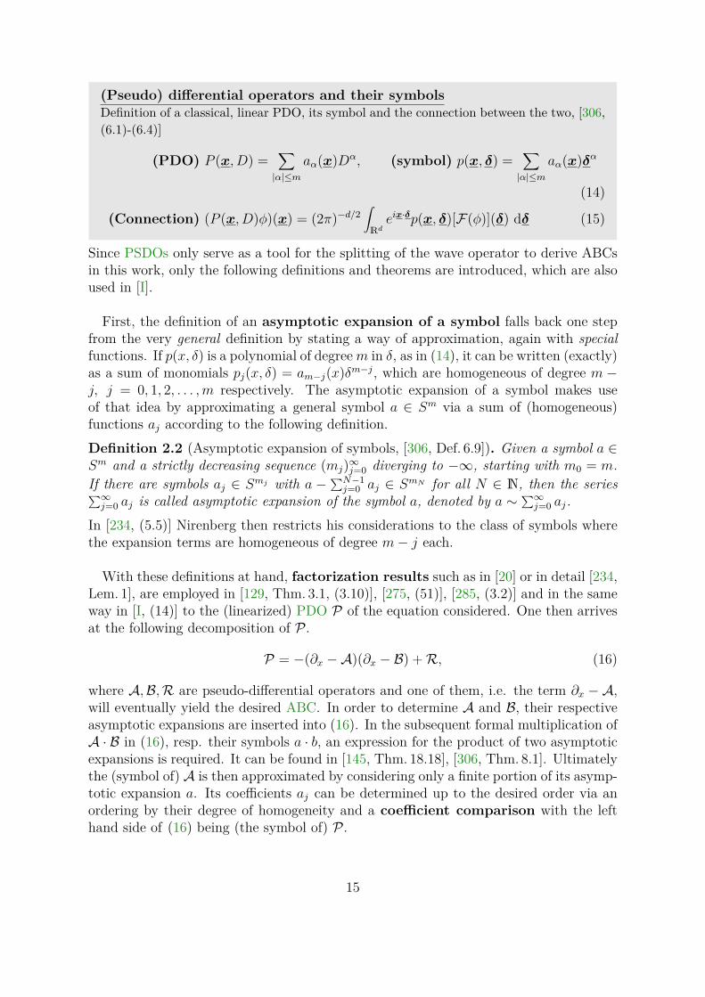
(Pseudo) differential operators and their symbolsDefinition of a classical, linear PDO, its symbol and the connection between the two, [306,(6.1)-(6.4)]

(PDO) P (x, D) =∑|α|≤m

aα(x)Dα, (symbol) p(x, δ) =∑|α|≤m

aα(x)δα

(14)

(Connection) (P (x, D)φ)(x) = (2π)−d/2∫Rdeix·δp(x, δ)[F(φ)](δ) dδ (15)

Since PSDOs only serve as a tool for the splitting of the wave operator to derive ABCsin this work, only the following definitions and theorems are introduced, which are alsoused in [I].

First, the definition of an asymptotic expansion of a symbol falls back one stepfrom the very general definition by stating a way of approximation, again with specialfunctions. If p(x, δ) is a polynomial of degreem in δ, as in (14), it can be written (exactly)as a sum of monomials pj(x, δ) = am−j(x)δm−j, which are homogeneous of degree m −j, j = 0, 1, 2, . . . ,m respectively. The asymptotic expansion of a symbol makes useof that idea by approximating a general symbol a ∈ Sm via a sum of (homogeneous)functions aj according to the following definition.Definition 2.2 (Asymptotic expansion of symbols, [306, Def. 6.9]). Given a symbol a ∈Sm and a strictly decreasing sequence (mj)∞j=0 diverging to −∞, starting with m0 = m.If there are symbols aj ∈ Smj with a −∑N−1

j=0 aj ∈ SmN for all N ∈ N, then the series∑∞j=0 aj is called asymptotic expansion of the symbol a, denoted by a ∼ ∑∞j=0 aj.

In [234, (5.5)] Nirenberg then restricts his considerations to the class of symbols wherethe expansion terms are homogeneous of degree m− j each.

With these definitions at hand, factorization results such as in [20] or in detail [234,Lem. 1], are employed in [129, Thm. 3.1, (3.10)], [275, (51)], [285, (3.2)] and in the sameway in [I, (14)] to the (linearized) PDO P of the equation considered. One then arrivesat the following decomposition of P .

P = −(∂x −A)(∂x − B) +R, (16)

where A,B,R are pseudo-differential operators and one of them, i.e. the term ∂x −A,will eventually yield the desired ABC. In order to determine A and B, their respectiveasymptotic expansions are inserted into (16). In the subsequent formal multiplication ofA · B in (16), resp. their symbols a · b, an expression for the product of two asymptoticexpansions is required. It can be found in [145, Thm. 18.18], [306, Thm. 8.1]. Ultimatelythe (symbol of) A is then approximated by considering only a finite portion of its asymp-totic expansion a. Its coefficients aj can be determined up to the desired order via anordering by their degree of homogeneity and a coefficient comparison with the lefthand side of (16) being (the symbol of) P .

15

Angle-adaptive ABCs for Westervelt’s equation - Contribution of [I]: In this ar-ticle absorbing boundary conditions for the potential form of the Westervelt equation(8) are derived using methods from pseudo differential calculus. First, they form anextension to the classical EM conditions taking into account the nonlinear term similarto [275]. However, additionally the angle of incidence is considered in the derivation. Incontrast to the approach of [133], where a predefined set of angles with optimal absorp-tion properties is chosen, in [I] the angle of incidence is adaptively computed and thendirectly inserted into the respective boundary condition formula. An efficient algorithmfor the computation of the angle of incidence is stated with further method parametersfor fine tuning. Different linearization strategies for the nonlinear part of the equationare compared, where one specific variant outperforms the others by far. The condi-tions are tested and compared in 2D and 3D application relevant scenarios dealing withultrasound.

Perfectly matched layers: A different approach to the artificial boundary problemis summarized under the term of PMLs. Originally introduced by Berenger [36] forthe electrodynamic Maxwell equations, their basic idea consists of a highly damping“sponge”-layer encasing the truncated computational domain Ω at all artificial bound-aries. Within that layer, waves are damped to non-critical amplitudes such that theirreflections coming from the very outer (outside of the encasing layer) boundaries canbe neglected. On those very outer boundaries classical boundary conditions such asDirichlet can be used then. The mathematically challenging part in the derivation ofPMLs however is not the mere introduction of an additional damping parameter σ,which is then just chosen wide enough. On the interface between Ω and the PML, hencebefore damping to negligible amplitude, reflections can originate if the impedance differ-ence between the two materials is not zero. Hence the PML’s material has to fulfill animpedance-matching condition with the interior material in addition to its dampingproperty. In one dimension this can be achieved by extending from real to complex mate-rial parameters and choosing for example ρpml = ρ(1− iσ) and cpml = c

1−iσ [170, (5.139)].This results in a match with the interior material’s impedance Zpml = ρpmlcpml = ρc = Zas well as a damping of the wave by the factor e−σx with x being the depth of the wave-front within the PML. In two and three dimensions again the angle of incidence plays arole, which is resolved by splitting even scalar fields such as pressure into artificial spatialcomponents treating each of them with their own damping parameters according to theone dimensional result. A further strategy to increase the damping provided within thePML while retaining the matched impedance at the interior-PML interface is to applythe impedance-matching condition to determine the damping coefficients at the interfaceand then smoothly increase them towards the outer boundary [36]. For a PML layer ofwidth L this results in a decrease of the outgoing wave’s amplitude by ∼ e−2

∫ L0 σ(x) dx

until it reenters Ω. Specifically for the acoustic case derivations can be found in [170]and in combination with the Helmholtz equation also in [228] employing an analyticalcontinuation of the plane wave solution and a coordinate transformation, also see [61,158, 252]. An application of PMLs to a nonlinear wave equations is discussed in [16].

16

2.3. Elastic solid modelThe equations of linear elasticity form the second mathematical model that is part ofthis thesis. [II] studies the interplay of the elastic wave-equation when coupled to theacoustic models from before and gives convergence results for the numerical solution ofthe resulting coupled system. [III] then considers the problem in an applied case-studyfrom seismology where additional model components such as special source mechanismsare added. A background about those additional factors directly relating to the seismicmodeling is given in Sec. 2.4, while here in Sec. 2.3 general foundations of linear elasticitytheory are presented.

Derivations from continuum mechanics: The equations of static (linear) elastic-ity can be derived from continuum mechanical considerations [90] such as the conser-vation of mass and (angular) momentum in combination with a constitutive materiallaw describing the material internal stress-reaction to deformation. Employing a dis-placement base approach, the base variable is the displacement vector field u fromwhich the strain-tensor E = 1

2

(∇u+∇u> +∇u · ∇u>

)and the linearized strain-

tensor ε = 12

(∇u+∇u>

), neglecting the geometric nonlinearity ∇u · ∇u> are formed,

where this geometric linearization is valid for relatively small displacements. So far, allinvolved quantities are valid for arbitrary materials as they only contain given defor-mations. The question arises, what internal stresses, i.e. forces per infinitesimal area,are created in a specific material subjected to deformations. It was Cauchy who provedin 1822 [22, 278] that the answer can be given in terms of a symmetric stress-tensor σallowing to compute internal forces acting over virtual cut-surfaces via F =

∫Γ σ ·n dS.

It remains to specify the relation between strain ε and stress σ. Here the choice ofa linear relation in the form of Hook’s law σ = C : ε with the fourth order materialtensor C results in linear elasticity theory. Symmetry considerations depending on theinternal structure of the material in use reduce the amount of free parameters withinC [72]. While organic materials such as wood or bones might for example be mod-eled by an orthotropic material law [143, 265] respecting some e.g. fiber-orientation,isotropic materials, without any preferred direction, state the most simplest case. Bythe Rivlin-Ericksen theorem [67, Thm. 3.6-1, 3.8–1] for such an isotropic material ten-sor only two free parameters are left, ultimately leading to the linear, homogeneous,isotropic material law σ(u) = 2µε(u) + λ(∇ · u)I, where the parameters λ and µ arecalled Lamé-parameters. Returning to the continuum mechanical conservation laws, thestate equation (17) is derived, where f denotes some external (volumetric) force andsuitable boundary conditions have to be prescribed. This could be Dirichlet conditionsin case of a fixed/prescribed displacement u = g, homogeneous Neumann conditionsσn = 0 in case of free surfaces, elasto-acoustic coupling conditions (cf. Sec. 3.3) orabsorbing boundary conditions specifically tailored for elastic waves (see below).

17

Elasticity equations:Equations used for the modeling of solids, e.g. the transducer and tissue parts in [II] orthe earth’s soil layers in [III].

(Static) −∇ · σ = f (17)(Dynamic) ρu−∇ · σ = f (18)(Dynamic with damping) ρu+ 2ρζu+ ρζ2u−∇ · σ = f (19)

Seismic (moment) sources can be incorporated via f or directly by a modification of σ. ρdenotes the materials density, ζ is damping parameter.

In order to move from a static to a dynamic model, Newton’s second law F = mucan be employed to arrive at the elastic, second order in time, wave equation (18) whichthen of course needs to be supported by suitable initial conditions.

To incorporate damping or attenuation in the equation additional damping termsscaling with a damping parameter ζ, as used in [202] and the articles of this thesis, allowto specify frequency independent attenuation e.g. in each soil layer of the earth’s crustas in [III]. The parameter ζ is related to the materials quality factor Q = 2π E

∆E [9, 286]expressing the relative energy decay of a wave per wavelength. The damping approachcan also be related to the PML technique mentioned in Sec. 2.2 damping the wholewave-field with a defined attenuation factor [55, 194], however, in contrast to the outerPML-layer, extended to the whole interior region. It is furthermore advantageous from acomputational perspective as in the semi-discrete form of the equation it only introducesscalar multiples of the mass matrix being diagonal in the spectral element method, seeSec. 3.1. Hence, almost no additional numerical effort has to be invested. Anotherfamous method to introduce damping would be by means of Rayleigh-damping [206].The resulting model equation (19) states a relatively simple model that, considering allthe uncertainties involved in real seismic applications such as the distribution of soilmaterials or fault parameters, is still often used due to its computational advantages.The model can be extended in various directions e.g. by means of different constitutivelaws involving not only elastic but also plastic models [113, 184, 200, 236], or by meansof visco-elastic/hysteresis based attenuation models [42, 83, 205] such as the Maxwell-or Kelvin-Voigt-model introducing certain degrees of nonlinearity into the equation.

ABCs for elastic waves: The dynamic elasticity equation (19) is a vector-valued waveequation. As such, the same requirements on absorbing boundary conditions to copewith artificially truncated domains as in the acoustic case arise. Results very similar to[95] in the acoustic case can be found also by Engquist and Majda for the elastic casein [94]. Also very similar to the acoustic case Higdon generalizes the angle dependentconditions from [133] to the elastic case in [135, 136]. [120] supports such conditionswith further numerical experiments in the finite element setting. A common idea in thederivation of ABCs for elastic waves is the splitting of the displacement wave field intotwo components being normal and tangential, resp. pressure- and shear-waves, each

18

propagating with its own velocity cn, resp. ct. To each of them e.g. the simplest 0th-order EM conditions (10) can then be applied with the respective value of c [207]. Ashort derivation of these two wave components which is of special relevance for seismicapplications is given in Sec. 2.4. Finally, as in [9, 57, 216] the articles of this thesis use theabsorbing boundary conditions proposed by Stacey [280], who combined the individualterms for normal and tangential wave-components in order to find correction terms thatimprove the order to the ABCs w.r.t. to the incidence angle without requiring higherorder derivatives.

2.4. Seismic modelingThere is a number of special properties and additional methodology to linear elasticitythat becomes especially useful in certain areas of application. For the seismology part,I will highlight two of them. First will be the decomposition of the dynamical elasticityequation into its pressure- and shear wave components, which already played some im-portant role in the derivation of ABCs for elastic wave propagation. Second, there willbe shortly summarize the seismic source mechanisms that were used e.g. in [III].

P- and S-waves, elasticity revisited: In contrast to pure, longitudinal pressure (P)-waves as they occur in acoustic media like water or air, the elastodynamic wave equation(18) (for this section the additional damping terms of (19) and the external force f will bedropped) allows for a second propagation mechanism being transversal shear (S)-waves.The two wave components propagate with different, material dependent velocities thatare denoted by cP and cS. The distinction of these two wave types is important as forexample in case of an earthquake their wave speeds can differ by a factor of 1.5 - 2, see forexample [288] with P-waves arriving prior to S-waves. Derivations of that splitting canbe found in [272], or [152, Chap. 2], where equation (18), with the linear, homogeneous,isotropic material law for σ(u) inserted, is transformed using vector identities to obtain:

ρu− (λ+ 2µ)∇(∇ · u) + µ∇× (∇× u) = 0 (20)assuming potentials (Φ,Φ×) for a Helmholtz-decomposition of u = u + u× into arotation free component u = ∇Φ and a divergence free component u× = ∇×Φ× onecan see (20) as the superposition of the two independent potential-waves:

Φ −λ+ 2µρ

∆Φ = 0, Φ× −µ

ρ∆Φ× = 0 (21)

the first traveling with cP =√

λ+2µρ

, the second with cS =√

µρ. Often seismological soil

material datasets contain these speeds instead of other material parameters, where thelarger one of the two, cP , is also used e.g. for the computation of the Courant-Friedrichs-Lewy (CFL)-number within a simulation.

19

Seismic source mechanism: With the dynamic elasticity equation (19) describing thepropagation of seismic waves, it remains the question how to model the source/origin ofsuch waves, resp. an earthquake. For a general, first understanding of earthquake sources[291, Chap. 1] summarizes underlying physical mechanism taking place at a seismic fault,i.e. a (two-dimensional) crack in the solid earth’s body where the body parts on eitherside of it slide parallel to each other due to a sudden release of accumulated stress.A seismic fault can be approximated by a e.g. rectangular fault-plane of area A withorientation being defined via the azimuth-angle φ w.r.t. north and the dip-angle δ w.r.t.a horizontal plane. Distributed over the fault plane one then defines the slip vectorfield s. It describes how far each material point on the fault plane has moved comparedto its (former) counter part on the other side of the fault. A measure for the intensityof an earthquake is given by the overall seismic moment M0 = µsA [4, 5], where s isthe mean slip and µ the shear modulus of the material. From M0 also the publicly wellrecognized (moment magnitude) scale valueMW = 2/3 log10(M0)−10.7, associated withthe severity of an earthquake, can be computed [5, 171].For the mathematical modeling of the fault one generally distinguishes [264] on the

one hand side dynamic rupture models resolving the rupture-process [75, 244, 293] andthe resulting slip involving e.g. friction models. On the other hand side, there arekinematic rupture models, where these data are already given, e.g. by measurement dataand/or other models, and only the wave propagation into the rest of the domain duringthe predefined rupture process is numerically computed. In [III] the later approach isemployed to recreate a realistic earthquake relying on the broad range of fault dataobtained from [290]. In detail that data is used in the source models described in [103]especially with the seismic-source-tensor/stress-glut model [24],[291, Chap. 5]. Theidea of the model is to incorporate the non-elastic stress contributions, e.g. induced bythe slip vector-field s on the fault-plane with normal n into a seismic moment tensorm = (mij(x, t))3

i,j=1 depending on the spatial location x and time.

(Seismic moment tensor) m(x, t) = m0(x) ·m(t)(t) ·[(s⊗ n) + (s⊗ n)>

],

where m0 scales with the magnitude of the earthquake and m(t)(t) is the moment releasefunction associated with the time-evolution of the rupture process. The seismic momenttensor, resp. its equivalent body force f = −∇ ·m [103], models the stresses thatare induced in the surrounding material by the non-elastic slip caused by the ruptureprocess. These are then used to startle a wave propagation from the fault plane intothe rest of the computational domain eventually attaining a displacement field thatis again in equilibrium with the the overall stress being the sum of elastic and non-elastic/prescribed stresses.For specific earthquakes, fault-plane data such as the moment-distribution m0(x) or

the slip-vector field s [290] can be obtained by seismic wave-form inversion techniques[132, 156] relying on actual measurement data such as they are provided by [1] for theregion of Turkey considered in [III]. The situation is more complex if one tries to simulatealternative, however still realistic scenarios that have not (yet) happened. This is donefor example in the seismic risk assessment [13], also see Sec. 3.4 of a region by means

20

of physics based simulations, where several possible scenarios with different parameterdistributions are simulated. In order to conduct such random simulations with sensibleparameters, correlations between fault parameters have been analyzed e.g. in [73, 264]from which reasonable choices of parameters can be deducted.

2.5. Further mathematical toolsIn this section I will briefly state a small selection of mathematical tools/theorems thatare mainly used in the proofs of the articles constituting this thesis.

Young’s ε inequality Young’s ε inequality is a variant of the standard Young inequalityinvolving a parameter ε. By choosing ε either very large or very small, it allows to controlone of the terms on the right hand side.

Lemma 2.2.1 (Young’s ε inequality [105, App.A]).Let a, b ∈ R and ε ∈ R>0, then there holds:

ab ≤ a2

2ε + εb2

2 (22)

This becomes relevant in situations where one wants to absorb e.g. the a2 term on theright by some additional term Ca2 on the left, where C > 0 is an unknown constant. Inorder to avoid rendering the left hand side negative, one has to choose ε large enough suchthat 1

2ε < C. Then the term can be brought to the left hand side easily. Of course thechoice of a large ε increases the b2 term on the right hand side, which again emphasizeswhy only one term can be controlled by that approach. This fact, in combination withthe common saying “You have to rob Peter to pay Paul” also yields the name Peter-Paulinequality to (22) [84].

Gronwall’s lemma For the lemma of Gronwall a lot of different versions exist. Theircommon purpose is that they allow to derive from an implicit estimate ϕ(t) ≤ F (t, ϕ) ofsome quantity ϕ an explicit estimate ϕ(t) ≤ C(t), where F typically involves integrationand C grows with time. The lemma is employed, e.g., in stability estimates for timedependent problems.

Lemma 2.2.2 (Gronwall’s lemma [250, Lem. 2.2]).Let a, b ∈ R, b > a and A,B, ϕ : [a, b] → R where A ∈ L1(a, b) is non-negative, Band ϕ are continuous and B is non-decreasing. Then the implicit estimate

ϕ(t) ≤ B(t) +∫ t

aA(τ)ϕ(τ) dτ, ∀t ∈ [a, b],

implies the explicit estimate

ϕ(t) ≤ B(t) exp(∫ t

aA(τ) dτ

), ∀t ∈ [a, b].

21

Banach’s fixed point theorem Banach’s fixed point theorem plays an important rolein proofs dealing with nonlinear equations as for example the a priori error estimatein [II, IV], where it guarantees the existence of a solution to a nonlinear problem, alsosee for example [232, 240]. The typical procedure therein first assumes a linearizedversion of the nonlinear problem around a reference solution. If for example u would bethe exact solution of the (nonlinear) PDE, one might choose a finite element functionwh that is, in some energy-norm ‖ · ‖E, “close to u”, i.e. ‖u − wh‖E . hr for somer > 0, as such a reference solution. With u(wh)

h being the solution of the resulting linearproblem one finds an estimate like ‖u− u(wh)

h ‖E . hr + ‖f(u)− f(wh)‖. Here the laterterm ‖f(u)− f(wh)‖ contains differences from the nonlinear terms f resulting from theuse of the exact solution u vs. the use of the linearization wh. This estimate howeveralso still depends on wh. In order to get rid of wh one carefully defines a mapping Sthat maps the reference solution wh onto u(wh)

h . A fixed point of such a mappingwould then constitute a finite element function zh with ‖u − zh‖E = ‖u − S(zh)‖E .hr + ‖f(u) − f(zh)‖. From here it becomes visible that the last term involving thenonlinear terms f must be bounded somehow by Chr in order to carry over the error-estimate from the linear to the nonlinear model as well as to show contractivity of themapping S as it is needed in Banach’s fixed point theorem 2.2.1 that guarantees existenceof such a fixed point.

Theorem 2.2.1 (Banach’s fixed point theorem [302, Ch. IV.7]).Let (X, d) be a complete metric space and let M ⊂ X be non-empty and closed. If amapping S : X → X fulfills:

• Self-mapping property: S(M) ⊂M

• Contractivity: d(S(x),S(y)) ≤ L · d(x, y), ∀x, y ∈M with L < 1

thenM contains exactly one fixed-point x∗ of S, i.e. S(x∗) = x∗. Furthermorethe sequence xn+1 := S(xn) with x0 ∈M being arbitrary converges to x∗ with:

d(xn, x∗) ≤Ln

1− Ld(x1, x0)

While existence of such a fixed point can then directly be guaranteed by means of Ba-nach’s fixed point theorem, the challenging task to be done is the proper definition ofthe set M and the mapping S and to proof the prerequisites necessary for the appli-cation of the fixed-point theorem, being the self-mapping property and contractivity.Such remaining estimates on the nonlinear terms ‖f(u) − f(wh)‖ now rely on inverse-(Lem. 3.2.1) and interpolation-estimates (Lem. 3.2.3) from classical finite element, resp.DG literature.

22

3. Numerical methodsHaving introduced the mathematical models for acoustics and elasticity as well as sometheoretical foundations for the applied methods, this section focuses on the numericalmethods used to solve the resulting (systems of) PDEs.For the spatial discretization there will be summarized results, references and tools

about discontinuous Galerkin methods in Sec. 3.1, especially in connection with the spec-tral (element) method. Since all involved models are time-dependent, Sec. 3.2 containsan overview over Newmark-type time integration schemes that were used in this the-sis with special attention to the numerical damping of higher modes. In Sec. 3.3 theelasto acoustic coupling employed in [II, III] will be discussed. Sec. 3.4 gives an overviewover different applications and the internal structure of the high-performance software-framework SPEED that was mainly used for this thesis.

3.1. Discontinuous Galerkin spectral element methodThe method used for spatial discretization in articles [II, III, IV] is the discontinuousGalerkin spectral element method (DGSEM) as discussed in [14, 214], applied to themodel equations of elasticity [9, 13] and acoustics, where examples for the linear waveequation are given in [8]. The method is a combination of the classical spectral elementmethod (SEM) [54, 53, 273] using polynomials associated with Gauss-Legendre-Lobatto(GLL) quadrature nodes on hexahedral elements as finite element basis functions anda DG approach [81, 255], in detail the symmetric interior penalty Galerkin method(SIPG) [17, 304], that allows jumps across element faces. To some extend the faces,where the DG paradigm is applied and where a conforming approach is used instead,can be chosen by the user. While it is possible to treat every element face as a DG-face, resulting in a classical, full DG scheme, the idea of DGSEM is to partition Ωinto subdomains Ωi, i = 1, . . . , N , each meshed and treated in a conforming way usingspectral elements, while the DG approach is only applied at the subdomain-interfaces.This hybrid approach combines advantages from both continuous and discontinuousdiscretizations such as the lower number of degrees of freedom in the conforming andthe flexibility in meshing and local h- and p-refinement of the non-conforming approach.It further becomes especially useful in situations where a complex geometry consistingout of different materials, possibly spanning multiple length scales or having varyingaccuracy requirements, is considered. Prime examples for applications of DG, SEM andDGSEM can be found in seismology and the simulation of earthquakes [60, 88, 100, 193,191, 214, 216, 305], where such methods offer an attractive alternative to e.g. finitedifference schemes [195, 220, 221] and classical finite element approaches [37, Sec. 2]. Inthe rest of this section first some background information and definitions for the DGparts of the method are introduced working with an arbitrary elementwise polynomialbasis. Second, important inequalities such as trace-, inverse- and error-estimates aresummarized. Finally a short review on SEM is given, from which a specific elementwisebasis and numerical quadrature rule is employed to constitute the final DGSEM scheme.

23

Historical development of DG-methods: Following the introductory article [116, partI, article 5] and [18, 69], the DG method can be traced back to Reed and Hill [253], with anumerical analysis of [157, 201], considering a first order, hyperbolic transport equationarising from nuclear physics. In (one of) their formulations, the weak form of the equa-tion was already discretized using independent, elementwise degrees of freedom (DOFs)allowing for discontinuities in between. Applications also to elliptic and parabolic prob-lems, especially involving the SIPG method, which is also applied to the second orderspatial derivative part in this work, then followed [17, 26, 304]. Further developmentsrelated to DG methods include the weak incorporation of Dirichlet boundary conditions[235], a posteriori error-estimators [56, 99, 175] or shock-capturing methods and slopelimiters [146, 198, 289] also known from finite volume methods. Also see [19] for abroader overview over different DG techniques.By now DG methods have been applied to many different problems. From the afore-

mentioned seismic applications, over waves [78, 126, 147, 227], especially also nonlinearacoustic ones [182, 287], mostly via their conservative system formulation, the shallowwater equation [3] up to fluid-mechanics [118] and turbulence [31] and magneto-hydro-dynamics [300].

Meshing: For the rest of this section the Westervelt equation (8) will serve as a modelproblem in order to formulate fundamental parts of the method. The basis of a DG (orgeneral finite element) discretization of e.g. the model problem is formed by meshingthe domain Ω, i.e. forming a non-overlapping subdivision T = τkNk=1,Ω = ⋃N

k=1 τk,where the τk s can be simplices, quadrilaterals in 2D resp. hexahedra in 3D, or evengeneral polyhedra. In contrast to a conforming mesh, hanging nodes are allowed in aDG setting. As in classical finite elements, hτ stands for the diameter of the elementτ and by h := maxτ∈T hτ one denotes the maximal element diameter present in themesh. Further classical terms such as shape-regularity, i.e. the existence of a constantκ > 0 such that κhτ ≤ ρτ , ∀τ ∈ T , ρτ being the radius of the largest inscribed ballwithin τ , are defined for simplicial, but also general meshes for example in [81]. It setsin relation the element diameter hτ with the area resp. volume of the element and henceavoids degeneracy. For anisotropic elements that are e.g. very thin in only one direction[114, 115], for prismatic elements [51] or for even more general polyhedral elements, thatare of interest recently, [15, 50, 52, IV] state similar conditions and results. In [II] theDG approach is only applied on subdomain interfaces, as introduced in [14]. Therefurther mesh assumptions dealing with the comparability of the subdomain meshes areformulated.For the rest of this chapter E will denote the set of all element edges (2D) resp. faces

(3D) that are part of the DG approach. In case of the subdomain wise DG interfacecoupling, it will only contain the interface- and boundary-faces, in the full DG approach,it will contain all faces. With each face e ∈ E one associates the face normal ne beingeither the outward normal of the element on the left side of e, denoted by n+ or theoutward normal of the element on the right side of e denoted by n−, where the choice of“left and right” is arbitrary but fixed for each face. With the face normal at hand one

24

then defines the mean- and jump-values of a scalar quantity ψ as:

(Mean- and jump-values) ψ = 12(ψ+ + ψ−), [[ψ]] = (ψ+ − ψ−)ne,

where again ψ+ and ψ− stand for the values of ψ on the left resp. right hand side ofthe face, where on Dirichlet boundary faces the boundary value is taken instead of the“outer” evaluation. For vectorial or even tensorial quantities similar definitions can befound in [7, 9].

Variational formulation: With the non-conforming mesh Th also comes a broken defi-nition of the space Hn(Th) as well as the finite element ansatz space Vh, where the indexh denotes the dependency on a particular mesh with mesh-size h e.g. from a family ofsuccessively refined meshes. For the later, Pp(τ) denotes the space of polynomials upto order p over the element τ and Qp(τ) the space of polynomials up to order p perdimension over τ , which can be set up via a tensor product.

Definition 3.1 (Broken spaces). Let n, p ≥ 1 and Sp(τ) be either Pp(τ) or Qp(τ), thenthe broken space Hn and finite element ansatz space Vh in a full DG setting are definedas:

Hn(Th) := ψ ∈ L2(Ω) | ψ|τ ∈ Hn(τ) ∀τ ∈ Th

Vh := ψ ∈ L2(Ω) | ψ|τ ∈ Sp(τ) ∀τ ∈ Th

Again, in a subdomain-wise conforming approach with DG faces only at the interfaces,the spaces are defined differently as subdomain-wise H1 instead of only L2 [14, II].

Returning to the Westervelt equation (8) as a model-problem, its variational formusing the SIPG is stated in the following as an example. To that extend, the DGparadigm will be employed over the whole domain, i.e. assume every element as amaterial subdomain and hence all element faces are assumed to be DG interfaces. Forsimplicity of exposition the damping factor is chosen to be b = 0 with homogeneousDirichlet conditions assumed on all of ∂Ω and f ∈ L2(Ω) as a right hand side force term.

Definition 3.2 (Bilinear forms and penalty). The following bilinear forms are defined,where the gradient has to be understood in a broken, elementwise, sense:

• Interior bilinear form: ah : Vh × Vh → R, ah(ψh, φh) := (c2∇ψh,∇φh)Ω

• Consistency term: bh : Vh × Vh → R, bh(ψh, φh) := ∑e∈Eh〈c

2∇ψh , [[φh]]〉e

• Symmetry term: sh : Vh × Vh → R, sh(ψh, φh) := ∑e∈Eh〈c

2∇φh , [[ψh]]〉e

• Penalty term: ph : Vh × Vh → R, ph(ψh, φh) := ∑e∈Eh〈χ [[ψh]] , [[φh]]〉e

where the penalty parameter χ on the face e ∈ E is defined as χ|e := σmaxτ∈τ+,τ−c2p2

hτwith τ+ and τ− being the elements left and right of the face e and σ is constant to bechosen appropriately (large).

25

With these definitions and 2k = 2+B/Ac2 being a more compact notation for the nonlinear

coefficient, the semi-discrete variational form then reads:

(Semi-discrete variational form)Find ψh ∈ Vh such that for almost all t ∈ (0, T ) and for all φh ∈ Vh there holds:

(ψh, φh)Ω + ah(ψh, φh)− bh(ψh, φh)− sh(ψh, φh) + ph(ψh, φh) = (23)∫Ω

2kψhψhφh dx+ (f, φh)Ω

with initial conditions (ψh(0), ψh(0)) = (ψ0,h, ψ1,h) ∈ Vh × Vh.

Inequalities and estimates: Inverse inequalities and trace estimates are some of themain tools for the error analysis of DG methods. The main purpose of trace estimates liesin relating norms on element faces, e.g. stemming from the above introduced consistency,symmetry or penalty terms of the weak form with norms on the interior of the element,in order to arrive at a specific norm for the final error-estimate. Inverse estimates on theother hand estimate higher order Sobolev-norms of finite element functions/polynomialsagainst lower order ones. In the following the notation x . y is used standing for x ≤ Cywith some constant C > 0.

Lemma 3.2.1 (Trace and inverse estimates [81, Lem. 1.44, 1.46], [268, Thm. 4.76]).Let τ ∈ Th and ψh ∈ Sp(τ), then there holds:

Trace estimate: i) ‖ψh‖L2(∂τ) .1h

1/2τ

‖ψh‖L2(τ),

Inverse estimates: ii) |ψh|H1(τ) .1hτ‖ψh‖L2(τ), iii) ‖ψh‖L∞(τ) .

1hd/2‖ψh‖L2(τ)

where d is the spatial dimension of Ω.

Details as well as precise values for the constants - at least for simplicial elements - ofthe trace inequality are considered in [301], while for more general, polygonal shapedelements a variant can be found in [52].For interpolation estimates as in Lem. 3.2.3, but using for example the DG norm (24),

the trace of a non-polynomial function ψ, resp. its interpolation error ψ − Πpψ has tobe estimated on element faces as well. Therefore the following continuous trace estimatecan be employed. Such trace inequalities are not only restricted to DG methods but canalso be found for example in isogeometric analysis [102].

26

Lemma 3.2.2 (Continuous trace estimate [81, Lem. 1.49]). Let Th be a shape regularmesh, τ ∈ Th, e be a face of τ and ψ ∈ H1(Th), then there holds:

‖ψ‖2L2(e) .

(|ψ|H1(τ) + h−1

τ ‖ψ‖L2(τ))‖ψ‖L2(τ)

. hτ |ψ|2H1(τ) + h−1τ ‖ψ‖2

L2(τ)

Interpolation-estimates: Following the typical structure of finite element a priori errorestimates a decomposition of the error ‖ψ − ψh‖ of exact solution ψ and finite elementsolution ψh into an interpolation part ‖ψ−Πpψ‖ and an approximation part ‖Πpψ−ψh‖is employed. Here Πp is a suitable interpolation operator from H1(Th) to Vh which, inthe full DG setting, can be employed element-wise. In order to control the interpolationpart of the error the following interpolation estimates are needed, which can also befound in [II, Lem. 4.4] and [IV, Lem. 2].

Lemma 3.2.3 (Interpolation estimate [45, Thm. 4.4.4, 4.6.11, Cor. 4.4.7]). Let Thbe a shape regular mesh, τ ∈ Th and ψ ∈ Hn(τ). Then there exists an interpolationoperator Πp : Hn(τ)→ Sp(τ) such that with m := minn, p+ 1 there holds:

L2-estimate: i) ‖ψ − Πpψ‖L2(τ) . hmτ ‖ψ‖Hn(τ), n ≥ 0,H1-estimate: ii) |ψ − Πpψ|H1(τ) . hm−1

τ ‖ψ‖Hn(τ), n ≥ 1,L∞-estimate: iii) ‖ψ − Πpψ‖L∞(τ) . hm−d/2τ ‖ψ‖Hn(τ), n > d/2.

The aforementioned interpolation estimate on element faces can be found for example in[81, Lem. 1.59] and again [52] states similar results in the general polygonal case. Finally[45, Lem. 4.4.1] also states a stability estimate for ‖Πpψ‖Wk,p(τ), which is then used in[II, Lem. 4.5].

Finite element error-estimates: Having available the semi-discrete form (23) of themodel problem as well as the estimates and inequalities from above, a priori error-estimates can be derived. In the elliptic case of e.g. Poisson’s equation, the strat-egy consist of showing continuity and coercivity [81] of the bilinear form ah(ψh, φh) −bh(ψh, φh)− sh(ψh, φh) + ph(ψh, φh) from above w.r.t. the DG-norms:

‖ϕ‖2DG :=

∑τ∈T|ϕ|2H1(τ) +

∑e∈E‖√χ [[ϕ]] ‖2

L2(e) (24)

‖|ϕ‖|2DG := ‖ϕ‖2DG +

∑e∈E

he‖ ∇ϕ · ne ‖2L2(e)

For coercivity to hold true, it is required that the penalty parameter σ within thedefinition of χ is large enough [17, 116]. Lower bounds on σ to be actually large enoughcan be found in [96]. The elliptic case then proceeds by estimating the individual norm

27

contributions to the interpolation error-terms on the right hand side of

‖ψ − ψh‖DG . infφh∈Vh

‖|ψ − φh‖|DG ≤ ‖|ψ − Πpψ‖|DG

by means of the interpolation estimates of Lem. 3.2.3 as well as their trace-equivalentsby means of Lem. 3.2.2. Finally one arrives at

‖ψ − ψh‖DG . hm−1‖ψ‖Hn(Th), m = minn, p+ 1,

provided ψ ∈ Hn(Ω).For time dependent problems, the approach is similar, e.g. for parabolic equations

like the heat-equation [17, 256], or the (linear) scalar wave-equation [126] or elastic waveequation [15]. In order to account for the time evolution of the problem, the norm (24)used for the error-estimate is extended for example by ‖ϕ‖2

L2(Ω) to form a, now timedependent, energy-norm

‖ψ(t)‖2E := ‖ψ(t)‖2

L2(Ω) + ‖ψ(t)‖2DG +

∫ t

0‖ψ(s)‖2

L2(Ω) ds,

where the last term appears additionally in case of the Westervelt and Kuznetsov equa-tion, see [II, (4.1)]. In that energy norm then stability- and later also error-estimates arederived, typically by testing the weak form, resp. the error equation, i.e. the differenceof the variational forms with the exact and numerical solutions being inserted, witha suitable test function. Here partial integration in time and the lemma of GronwallLem. 2.2.2 play an important role to obtain estimates that are explicit in the energy(energy/stability-estimate) or the error (error-estimate).

Numerical analysis of nonlinear (elasto-) acoustics - Contribution of [II] and [IV]:Here the novel contribution of [II] and [IV] lies in the incorporation of the nonlinear term∫

Ω 2kψhψhφh dx, resp. its equivalent in case of the Kuznetsov equation (9) even involvinggradients ∑τ∈T

∫τ 2k′∇ψh∇ψhφh dx, of the variational form. The error-analysis is first

conducted for a linearization around a reference solution, where the nonlinear terms,evaluated at this reference solution, are treated as additional force contributions to theright hand side. By doing so, the linear version can be analyzed with standard methodsand results from literature, while the problematic nonlinear part is dealt with separately.The method of choice to extend the error-estimate to the nonlinear regime is by meansof Banach’s fixed point theorem (Thm. 2.2.1) and the procedure described in Sec. 2.5.The result shows that the method converges with the same order of h in the nonlinearcase as in the linear one, for both Westervelt and Kuznetsov type nonlinearities, resp.a combination of both. The result holds true for elasto-acoustic interfaces in the sameway as for acoustic-acoustic interfaces between subdomains of different materials.

28

Spectral (element) method: Even though there is of course a connection, one hasto distinguish between (globally) spectral methods and spectral element methods SEM.The first one is mainly attributed to Orszag during the 1970’s, where he used truncatedseries of orthogonal polynomials [237] or Fourier-series [238], i.e. globally smooth, mu-tual orthogonal basis functions - hence the name spectral - to represent the solution ofa PDE, see also the details in the more recent text books [53, 54, 123, 273]. Originallyrestricted to rectangular domain shapes the method was soon extended to more generalshaped domains via mappings and by coupling multiple patches [239], both being princi-ples also used for finite element meshes. Eventually it was a logical step to combine theflexibility of finite elements concerning general domain shapes with the spectral methodsadvantages such as spectral convergence [54, Sec. 5.1, 5.4] as it can also be found in thevery similar [80, Sec. 2.3.2, 2.4] higher-order p-FEM e.g. in [23], [268, Cor. 3.12]. Withthe finite element space Vh being defined in Def. 3.1, resp. its analogue for conformingfinite elements, it still remains to choose an (elementwise, polynomial) basis ψjp+1

j=1spanning that space. A sensible choice for this basis now poses the connection to theoriginal spectral methods, see also [312] for a detailed review of the development of themethod.In classical, conforming finite elements, Lagrange-polynomials associated with (equidis-

tant) Lagrange interpolation nodes on each element can be chosen. Stitched togetheracross element boundaries they yield globally continuous basisfunctions with local sup-ports. Applying a numerical quadrature rule with sufficiently high degree of exactnessto assemble mass- and stiffness matrices results in their well known sparse structure.These are properties one wishes to pass on to the spectral basis to be chosen. Start-ing in one dimension, a well known family of orthogonal polynomials are the Legendrepolynomials Ln ∈ Pn([−1, 1]), n = 0, 1, 2, . . . , p+ 1. Their roots (xi)ni=1 are known to bethe Gauss-Legendre quadrature nodes yielding the highest possible degree of exactness,2n − 1 resp. 2p + 1 for n = p + 1, for the associated quadrature rule. However, sincethe nodes xi lie strictly in the interior of [−1, 1], continuity across element boundariescan not be enforced, posing a problem if the DG approach is not employed between allelements but a partly conforming approach is used, see [II]. In that case the boundarypoints x = −1 and x = 1 are supposed to be interpolation nodes as well and a mod-ified (nodal) basis, based on the GLL nodes being the roots of (1 − x2)L′n−1, isused. The associated quadrature formula yields a reduced degree of exactness of 2n− 3,resp. again 2p − 1 for n = p + 1 [54] but the chosen basis has the desired propertiesfrom above. The resulting method is called (a version of) the nodal SEM [80, 292]. Onquadrilateral/hexahedral elements a simple tensor product approach is used to obtainthe GLL-grid also in more dimensions while for simplicial elements different approachesare analyzed in [243].

An important trait of the just created method, where quadrature and interpolationnodes coincide, is the fact that by choosing the Gauss-Lobatto quadrature for the nu-merical integration of the mass matrix, one automatically obtains a diagonal, lumpedmass matrix with much less computational quadrature effort than with standard el-ements thanks to the interpolatory property of the interpolation polynomials. It has

29

to be noted though that due to the aforementioned reduced order of exactness of theGauss-Lobatto-quadrature, a variational crime is committed by the numerical integra-tion of each mass-matrix entry comprising the reference-element integral of ψhϕh beingof degree 2p plus the Jacobian determinant of the element mapping. The effect on theconvergence order can be analyzed using the first lemma of Strang [98, Lem. 2.27], wherethe order of the quadrature error enters. For parallelpiped-shaped elements the quadra-ture formula is still “good enough” and no order reduction is inferred, while for generallyshaped elements a dependency on the dimension d enters with an order reduction ford ≥ 3 [89, Thm3.6., Rem. 3.3. and 3.4.], also see [210]. However, the underintegrationis performed on purpose [60, Sec. 5.1] as such a diagonal mass matrix goes hand in handwith explicit time integration schemes such as the leap-frog or explicit Newmark scheme[313, 314].

Even though the invention of the SEM is now mainly associated with Maday andPatera [312, Ch. 7.3], an earlier applications of the SEM, even though not yet called likethat, to a reservoir simulation can be found by Young [311]. Later applications to theacoustic waves [270, 313, 314] as well as seismic waves [190, 191, 192, 193, 222, 248],where the SEM is one of the most commonly used methods, followed. While in [II] theerror analysis for the DGSEM method is only conducted w.r.t. an h-refinement assumingfixed values of p, the degree-dependency is resolved e.g. in [245] for a diffusion-problemor in [7, 10] for elastic and acoustic waves.

3.2. Newmark-type methods for time integrationAfter spatial discretization of any of the acoustic models (6),(8),(9) one arrives at asystem of ordinary differential equations (ODEs) of the structure:

M u+ Cu+Ku+ T (u, u, u) = b (25)

where M,C and K are mass, damping and stiffness matrices, b is a right hand sidevector of possible external forces or Neumann data that might vary over time and spaceand T summarizes all nonlinearities present in the respective equation, see for examplethe model problem (23). The precise shape of T depends on the equation in use consist-ing out of up to two of the third order tensors T1[u, u, ·], T2[u, u, ·], T3[u, u, ·], T4[u, u, ·]each, see for example [170, p. 165 f.], [IV, (7.1)], [V, p. 181], or even further nonlinearitiesentering through nonlinear ABCs such as in [I, (33)]. Dirichlet data are incorporatedeither via a lifting, see [I, (33)], or in a weak sense, see [IV, (7.1)], also on the right handside. For brevity, homogeneous Dirichlet data are assumed in this section and withoutfurther notation the system (25) is considered only for interior, non-Dirichlet DOFs.Initial conditions are given for u and u as usual.

In order to integrate (25) through time, different options are available. One commonapproach is to transform the second order in time system (25) into a first order system,e.g. by introducing the new variable v := u. For first order systems a long list of time

30

integration methods can then be used ranging from classical Runge-Kutta methods [125,295], over linear multistep methods [30, 174] up to symplectic methods [208, 263] makinguse of the Hamiltonian structure of the resulting first order system. Especially when itcomes to nonlinear systems mixed methods consisting of implicit and explicit (IMEX)time stepping schemes are advantageous combining the stability of implicit methodsfor the linear parts and the fast evaluation of explicit ones e.g. for the evaluation ofthe nonlinear part [138]. Another class of methods are exponential integrators. Theyemploy a linearization of the nonlinear equation producing a nonlinear remainder termon the right hand side. The resulting ODE system with inhomogeneity is transformedinto an integral equation by means of the variation of constant principle. The result-ing integral involving a matrix exponential is then solved numerically by a quadraturerule. A review of such methods can be found in [139]. Considering spatially high-orderapproximations with error rates O(hp), p ≥ 5, classical Runge-Kutta methods aimingat the same order for the temporal error O(τ p), p ≥ 5 suffer from the Butcher-barriersresulting in a continuously growing effort to compute the necessary amount of stages toreach the respective order. Here the arbitrary derivative (ADER) methods are settled.With them the solution is expanded into a (temporal) Taylor-series around the currenttime-step. Then the higher-order time derivatives are expressed via spatial derivativessuch that upon evaluation of the Taylor-series at the new timestep the high spatial or-der of the method carries over to the temporal error [178, 266]. Even though acoustic,elastic as well as further wave-type equations have distinct features and differences, theyfollow the same general structure. Hence, a common framework for acoustic, elastic andelectromagnetic waves being discretized using the DG method in space with subsequentapplication of different time integration methods can be found in [140].Alternative approaches that solve the time-dependent equations not in a separate

spatio-temporal way exist as well. As an example methods that involve a combinedspace-time discretization are discussed in [11]. Here the time interval is divided intosub-intervals over which spatial discretization is done independently with a couplingacross sub-intervals by means of DG interfaces and jump-terms. For such a space-timemethod also see [82].Finally, the approach that is also used in the articles of this thesis is a predictor-

corrector scheme of Newmark type with nonlinear extensions directly operating on thesecond order equation as proposed in [141, 170]. Generalizations to cope with Gibbs-like high frequency overshoots at steep wave-fronts typical in nonlinear acoustics arediscussed as well in terms of the so called Generalized-α schemes [66].

Derivation of the Newmark scheme: The original method of Newmark [231], for-mulated in displacement u, velocity v = u and acceleration a = u, can be derivedby approximating a in between timesteps tn and tn+1 either as mean-value ofthe respective value an and an+1, their linear interpolation or for example a centeredstep function. Each of these choices leads to a different parameter value β in the re-sulting scheme below. In any case, an+1 is treated as an unknown, while all valuesare assumed to be known at the old timestep tn. The value of vn+1 is then obtained

31

via a numerical integration of a, where the parameter γ enters as a weighting fac-tor for the quadrature weights. The quadrature is repeated to obtain un+1 from thenumerical integration of v where the second parameter β enters. One obtains the re-lations (26), (27), where an+1 is still unknown. To compute it, the original ODE (25)is evaluated at the new timestep tn+1 with the predicted values upred and vpred beinginserted. This yields the (nonlinear) system (28) that remains to be solved for ex-ample via a fixed-point iteration using an and the predictions for u and v as initialvalues. One then iterates, with iteration index κ, the solution of the linear systemM∗an+1,κ+1 = bn+1 − T (un+1,κ,vn+1,κ,an+1,κ) − Cvpred − Kupred and the correctionsteps in (26),(27) until a sufficient termination criterion is met before advancing to thenext time step. M∗ is called the effective mass matrix. Details about the algorithm canbe found in [141] as well as, for its generalized-α form, in [V, Alg. 1] and [IV, Sec. 7.1].

Newmark-relationsPredictor Corrector scheme with initial predictions for u, v, then alternating solution ofthe linear system and correction using its solution an+1. γ and β are the Newmarkmethods parameters with classical choices γ = 1

2 , β = 14 .

Prediction and Correction equations

vn+1 = vn + ∆t(1− γ)an + ∆tγan+1 =: vpred + ∆tγan+1 (26)

un+1 = un + ∆tvn + ∆t22 (1− 2β)an + ∆t2

2 2βan+1 =: upred + ∆t22 2βan+1 (27)

Algebraic system

M∗an+1 + Cvpred +Kupred = bn+1 − T (un+1,vn+1,an+1) (28)

The matrix M∗ is given by M∗ = M + γ∆tC + β∆t2K

For the special choice of parameters γ = 12 and β = 0 the method becomes the Störmer-

Verlet, resp. Leapfrog method (with full timestep size) [128, Ch. I.1.4]. In that sense,the Newmark algorithm is a generalization of those methods which, for β > 0 adds animplicit component also to the u-update (27). It should be noted that also explicit ver-sions of the Newmark-scheme exist as in [121] or [148, 149], where the ODE is evaluatedat the new (unknown) timestep tn+1 only for the acceleration an+1 while for u and v thepredicted values are inserted. This results in an algorithm where instead of the effectivemass matrix M∗ only the original mass matrix M appears in the algebraic system tobe solved. Especially for spectral elements, see Sec. 3.1, where M is diagonal this yieldsa fast, explicit algorithm, however, in the general case of C 6= 0 with only a first orderconvergence [148] compared to the, see below, order p = 2 of the implicit, “original”Newmark-method. In [211, 314] further versions of the Newmark scheme are discussedand compared in the context of acoustic waves, in [315] for elastic ones.

32

Consistency and stability: The presence of the parameters γ and β in the Newmarkscheme yield the questions, for which values of them is the resulting scheme stable andconvergent with which order? In the linear case the question has been addressed in [124]by means of a modal decomposition and in [62, 121] by deriving a recursion relationfor the Newmark scheme, i.e. formulating it as a linear two-step method, then usingstability criteria from the theory of such. As a result, one obtains the following generalconditions [149].Consistency: If γ = 1

2 , the method is consistent of order p = 2, otherwise at leastof order p = 1. In the absence of damping, i.e. C = 0 in (25), the additional choice ofβ = 1

12 then even leads to order p = 4 consistency [121].Stability: If γ ≥ 1

2 , hence especially in the second order case, stability is uncondi-tional, provided β ≥ γ

2 , as it is the case for the classical choice of parameters. For valuesβ < γ

2 conditional stability is given, restricting the time stepsize w.r.t. the maximalpresent frequency of the oscillation, again see [149].An increase of the parameter γ beyond the value of 1

2 introduces artificial dampingto the system. Especially in the context of nonlinear waves such behavior is favoredsince the additional damping helps to cope with the aforementioned high-frequencyovershoots. For a given value of γ > 1

2 the choice of β = 14(γ + 1

2)2 yields an optimaldamping behavior [148]. However, recalling the above consistency condition on γ thehigher-mode damping comes for the price of a reduction to an order p = 1 method.In addition, damping is not only confined to the high frequency range but also affectsthe remaining spectrum ultimately preventing oscillations. A method that allows toapply the additional damping ideally only on those high frequency components whilenot, or at least less, affects the low frequency band, would be the searched for remedy.Generalized-α methods as employed in the articles of this thesis accomplish exactly that.

Generalized-α-schemes: The need for a method with the just mentioned damping,accuracy but also stability properties led to the development of a multitude of meth-ods very similar to the Newmark method e.g. the Hilber-Hughes-Taylor HHT-α [137]or Wood-Bossak-Zienkiewicz WBZ-α method [307]. The idea of these two consists ofevaluating the ODE (25) at the new timestep t(n+1) as in the Newmark method, butinstead of u(n+1) a linear combination of (1+α)u(n+1)−αu(n) (HHT-α) and similar withu (WBZ-α) is used, shifting the purely implicit equation a bit more to the explicit side.Chung and Hulbert [66] then combined these two methods into a mathematical frame-work with two additional parameters αm and αf consituting the generalized-α method.Indeed for specific choices of αm and αf the Newmark method or any of the other twomentioned schemes can be recovered. The derived scheme is consistent of second orderfor γ = 1

2 − αm + αf and unconditionally stable for αm ≤ αf ≤ 12 , β ≥

14 + 1

2(αf − αm).This allows to increase γ beyond 1

2 without losing second order accuracy as it was thecase with the standard Newmark scheme. Further more in [66] it is also shown that theparameters αf and αm can be expressed by one single free parameter ρ∞ ∈ [0, 1], whichrepresents the numerical high-frequency damping of the method with no numericaldamping at all (ρ∞ = 1) vs. immediate annihilation in only one timestep (ρ∞ = 0).

33

The algorithm parameters and conditions are compared between the generalized-α andits predecessor methods in [97, Tab. 1-3], where the high-frequency damping capabilityof the method as well as its consistency order have also been analyzed for certain non-linearities, see also [43].Generalized-α methods have already been applied to (nonlinear) wave problems e.g.

in solid mechanics [44, 85, 150] and nonlinear (vibro) acoustics [258, 298] e.g. in aircraftsimulations [271]. There are also versions of the method extended to first order systemsby employing the idea of linear combinations between new and old timesteps in a simi-lar way with order and stability conditions also carrying over from second to first order[154]. Exemplary applications are in fluid-mechanics [154] or to phase-field models [122].Just recently also a 3rd order version of the method was derived in [33], with even higherorder versions for different types of equations following [32, 34, 35]. The precise wayhow the generalized-α method is used to resolve the steep wave fronts of the nonlinearacoustic models in this thesis can be found in [IV, Sec. 7.2], [V, Alg. 1].

3.3. Elasto-acoustic couplingIn the simulation of complex (mechanical) systems different materials, each with its ownphysics and modeling-equations, interact with each other. Formerly individual fields suchas displacement, pressure or temperature now exhibit dependencies, which need to becaptured by appropriate coupling mechanisms. One distinguishes between the couplingof variables once on the same domain Ω, such as acoustic potential and temperature in[257, 277] or a flow equation such as the Navier-Stokes system and a convection-diffusionconcentration/heat equation in fluid mechanics [79, 172, 223] influencing each other onthe whole volume of Ω; and second the coupling of different (material) regions over aninterface, as it is classically done for example in fluid-structure interaction [107, 261].Also for the coupling of an elastic to an acoustic material the later, interface-basedapproach is commonly used as the materials are usually separated. In the presentedexamples the elastic materials are a solid ultrasound excitator, a portion of humantissue, the earth’s ground or a building structure, while the acoustic material is mostoften a fluid such as water or air. In the elastic and acoustic linear case the problem istreated for example in [7, 106] with further, more elaborated simulation results in [8],where the key concept to transport information from one material domain to the otheris an exchange via interface conditions. The conditions are chosen in such a way thatcontinuity of (particle) velocity and normal stresses is given across the interface.In that sense the interface conditions avoid the penetration of one material into theother and hence keep the interface intact. Making use of the definition of the acousticpotential ψ (5) relating it to pressure p and particle velocity v, these conditions, withoutdamping, read:

(Interface conditions) σ(u) · n = −ρψn, ∇ψ · n = −u · n

where the first one can be identified as a Neumann-condition on the solid displacementfield u for equation (19), the second one in reverse is a Neumann-condition for the acous-

34

tic wave equation in ψ. While the interface conditions can be kept the same also in thepresence of the nonlinear terms of e.g. Westervelt’s or Kuznetsov’s equation, for the in-corporation of the additional damping term b∆ψ, see (8), (9), the conditions have beenextended in [II]. Similar interface conditions that have been extended even more to alsoincorporate nonlinear contributions can be found in [298] with the presented conditionsas a linear approximation.

For the solution process of the coupled system with its mutually dependent cou-pling conditions, a staggered time integration approach is well suited. Time integra-tion schemes of the Newmark family for the acoustic part discussed in Sec. 3.2 are ofpredictor-corrector type. Combining them also with such a scheme for the elastic part,as for example the leapfrog scheme allows for a sequential solution process where the in-terface conditions for the first variable can be evaluated from the predicted values of theother allowing for an explicit time integration approach. Wrapping the solution processinto an outer fixed point iteration loop as well as local time-stepping for only one of thetwo variables [277, III] are further options, easy to realize. Noting, that SPEED alreadycontained routines dealing with e.g. interface quadratures coming from the coupling ofelastic-elastic interfaces between non-matching grids [14, 214], the incorporation of theelasto-acoustic interface via boundary-conditions is straight forward for non-matchinginterfaces as well. Alternative approaches using Lagrange-multipliers for the interfacecoupling can be found in [106, 203].

Transducer-Fluid-Tissue simulation - Contribution of [II] part 2: From a modelingand applicational point of view the simulations conducted in [II] are of interest as theycontain the whole propagation process of a focused ultrasound wave. Starting with thecurved transducer mechanical impulses are applied to excite an elastic wave. Then thefirst elasto-acoustic interface transmits that wave into an ultrasound wave-guide whereit propagates according to the nonlinear acoustic models showing the typical effectssuch as wave-steepening. Finally the wave enters a portion of human tissue for whichdifferent, elastic and acoustic models are used. In that way, the conducted numericalexamples pose a further step in the simulation of medical ESWL, as it was one of thefirst motivations for this thesis.

3.4. Seismic simulations in SPEEDThe software framework SPEED is mainly developed at the MOX laboratory for Mod-eling and Scientific Computing at Politecnico di Milano in Italy, with strong influencefrom the older software GeoELSE [282, 283]. The acronym SPEED stands for SPectralElements in Elastodynamics withDiscontinuous Galerkin, which shows its original scopebeing in the simulation of (purely) elastic problems by means of the DGSEM approach[14]. This of course changed over time with SPEED now being able to handle also thenonlinear acoustic equations discussed in this thesis [IV] and coupled elasto-acousticproblems [7, II].

35

Features and application scenarios: The main area of application for SPEED liesfor sure in the simulation of seismological scenarios. Studies conducted so far encom-pass ground-only cases, however with a complex sub-soil layer structure, e.g. in theNetherlands [242], in combination with a seismic risk assessment in China [13] or atopography-including case in Italy [101]. However, also ground-structure interactionswere considered for example in [180, 209, 214, 216] for China, New Zealand and againItaly. Also for a different region of Turkey than in [III] a study was already conductedwith it [153]. In that sense, the case study of the Tahtalı dam in [III] queues up in along range of other scenarios on which validation of the SPEED code was repeatedlyperformed. It brings together the new elasto-acoustic coupling features by consideringthe full 3D interaction of the dam with the reservoir-lake behind it, the dam as a morecomplex fully resolved building structure as well as its embedding into a real topogra-phy. Making use of the rich set of available real-life data in the presented scenario makesthe article [III] a good showcase of SPEED’s capabilities in terms of large, complexsimulations involving real data. The DG approach is utilized in [III] to great extendin a full source-to-site simulation including the seismic fault model from Sec. 2.3 on akilometer scale as well as the, comparably much smaller scaled, dam. The multiscalenature of the problem is resolved by locally refined sub-meshes (h- and p-variability)that are coupled using DG interfaces as in [216, II, IV].The output data of the simulation are of importance from a seismological and en-

gineering perspective especially concerning peak values of displacement, velocity andacceleration [58, 92, 309]. Those values, presented e.g. in peak-ground maps such as in[III], are crucial for the assessment of seismic risks. Other quantities of interest mightbe the deformation, (maximum) displacement or frequency and spectral responses spec-tra (of a building) or stress and elastic pressure values, all being extractable from thenumerical simulations [104]. Building structures for example might be designed to resistground motions up to a certain percentage of the earth’s acceleration g ≈ 9.81 m

s2 beforetaking damage or even collapsing [13, 93]. Often, the buildings themselves are simulatedusing single- or multi-degree of freedom spring and damper models [93, 196], but alsofinite difference and finite element models are used [180, 215], especially for large, non-filigree buildings such as dams [176, 299], also under consideration of the dam-reservoirinteraction [6, 117].

Seismic dam simulation - Contribution of [III]: The case study performed in [III] pro-vides a detailed numerical study of the considered seismic event. The large scale simu-lation containing the actual seismic fault, modeled with the equations from Sec. 2.4, aswell as the analyzed building structure does not depend on additional assumptions onthe wave excitation such as a single backtraced seismogram measurement which, how-ever, is also used for a comparison. The whole simulation workflow is contained in onelarge, coupled multi-scale model, incorporating specific site effects such as the materialproperties of soil layers, topographic information, the dam geometry as well as the influ-ence of the reservoir lake. The simulation is validated by comparison of the numericaldata with actual seismogram readings at several locations, see [III, Fig. 8]. Altogether,

36

the simulation capabilities created and shown in this work offer a robust, accurate andcomputationally efficient numerical model for the assessment of the seismic response ofdam structures, involving various physical aspects. Due to its mathematical generality,in the future, it can also be employed at different locations for different scenarios.

Based on the simulation results such as peak values of quantities of interest andstatistical consideration concerning the probabilities of occurrence of certain (magnitude)events [142, 262], it is also of interest to conduct projections of other possible scenariosthat might happen. This ultimately leads to the field of seismic hazard analysis [71, 153,281, 296], which also poses a possible further field of research after completion of thisthesis.

Internal, (parallel) structure of SPEED: The core of SPEED is written in (proce-dural) FORTRAN and designed for parallelization using MPI (OpenMPI [111]) fromtop to bottom. SPEED follows a domain decomposition approach by dividing the meshinput using METIS [177] among the specified number of MPI ranks by partitioning theelement-based graph using an edge-cut minimization, which allows to keep the commu-nication volume between the different ranks low. The mesh itself can be generated byan arbitrary third party software such as for example Cubit [40] with standard exportcapabilities to e.g. EXODUS files, which are then suitably converted. In order to usethe tensor-product structure of spectral elements in SPEED, hexahedral elements arerequired. The creation of such hexahedral meshes can be challenging for complex geome-tries such as in [III]. It can be suitably achieved by a semi-automatic pave-and-sweepapproach [38, 39, 218] with details for the presented case being given in [III].All steps involved in time integration, from the initial assembly of matrices, setup

of initial conditions, prediction, correction, evaluation of boundary conditions up tothe diagonal solver (e.g. in case of a diagonal matrix to be inverted) are executed oneach rank in parallel with the necessary information exchange across the rank’s mesh-portion’s boundaries in between. For solver tasks that go beyond a diagonal-divide, e.g.for non-diagonal matrices as they appear in the Newmark-method once the matrix to beinverted also contains the stiffness matrix, an interface to PETSc [27, 28, 29] is availablein order to use the huge variety of (iterative) solvers provided by it.Independently from the domain decomposition, SPEED allows to define material sub-

domains also called blocks. Of course a natural choice for such blocks are indeed differentmaterial components like soil layers of different mechanical properties or different fluidregions. However, this structure can also be exploited to facilitate locally h- and/or p-refined grids as the meshes of these sub-blocks do not have to coincide at their interfacesthanks to the discontinuous Galerkin approach [14, 214]. Finally the graphical output ofSPEED can conveniently be based on those material blocks as well by generating VTK[267] files with the desired data for each of the blocks individually, which can then beread and displayed using Paraview [21] also individually allowing to “switch on and off”individual material components of the solution for inspection.

37

SPEED is by far not the only high performance computing (HPC)-oriented softwareused for seismic simulations. While SPEED has historically grown mainly from physicaland engineering applications such as different source and soil models and coupling (nowalso elasto-acoustic) methods, the software package EDGE incorporates techniques suchas fused simulations running multiple inputs at the same time [47, 49]. The realizationof such is not only interesting from a computer science point of view but yields also adesired feature for the aforementioned seismic risk analysis where multiple scenarios withdifferent sources need to be computed. EDGE as also SeisSol [46, 48] uses an ADER-DGmethod for time integration, also see the paper series [86, 87, 178, 179, 249]. In seismicsimulations also the finite difference method is still widely used, e.g. in the SW4- (SeismicWaves, 4th order) [215, 246] or FLAC3D-code [241]. In the light of advances in graphicsprocessing unit (GPU) computing, [76, 189] consider the seismic wave problem withGPU-bases implementations using finite differences resp. spectral elements. Finally [151]gives a review over the development of different methods, problems and applications.

4. Summary of results and outlookThe articles contributed deal with different topics of nonlinear acoustics and seismol-ogy ranging from a heuristic, methodological side in the derivation of the ABCs in [I],over the numerical analysis of its model equations in [II, IV] up to an application, cou-pled with optimization methods in [V] and an extensive, real-data driven computationalmodel and simulation case-study in [III]. The articles contain novel contributions in thesefields but also open new research questions and possibilities for future work. Closing thecircle to the originally asked scientific questions from Sec. 1.2 a short summary of resultsand outlook to further questions will be given.Beginning with [I] the ABCs derived therein for the Westervelt equation outperform

classical conditions by far, depending on the linearization strategy used in the derivation.Taking into account the angle of incidence is also of great importance for the qualityof the conditions. Therefore the introduced adaptive algorithm for the angle computa-tion provides an efficient, easy to use and implement option, where no a-priori knowledgeabout possible angles is necessary. Future work on absorbing boundary conditions mightinvolve their derivation for even higher orders, see e.g. [275], also for different modelequations, as well as their efficient implementation considering the higher order deriva-tives that come with them. Similar, the derivation of the shortly mentioned PMLs formore advanced nonlinear acoustics models is as well of interest in order to effectivelytruncate computational domains.In [IV] the purely acoustic problem, then in [II], with similar methods, the coupled

elasto-acoustic problem was discretized using the DGSEM approach. The model con-siders interfaces between elastic and acoustic materials as well as acoustic-acoustic in-terfaces with jumps in the acoustic material parameters. This allows for multi-materialsimulations such as the medically interesting, elaborated model example of an elasticultrasound transducer, an acoustic wave-guide and a portion of human tissue, where forthe later one different material models were compared. Using a linearization around a

38

reference solution and a fixed-point argument, it was proven that the method convergeswith the same order as in the linear case also for nonlinear acoustic models of Westerveltand Kuznetsov type in the presence of elasto-acoustic and acoustic-acoustic interfacesbetween different materials. Numerous, also computationally more intensive, numericalexperiments were performed to show the theoretically derived error-rates and to placethe considered model into the applicational context. That context being medical ESWLtherapy also links the works with [V], where the shape optimization of such an acousticfocusing device was conducted, increasing precision of an acoustic focusing lens. Dueto the need for high resolution approximations a lot of attention can be payed to therespective simulations with lens or transducer focusing as well as different model equa-tions in the future, also from a computational perspective applying methods from highperformance computing. Also a further development of combined models and simula-tions for example a thermo-(elasto)-acoustic one considering the effect of heat generatedby the focused ultrasound e.g. on tissue or a tumor might contribute to patient-specifictreatment [127, 257]. From a mathematical perspective the field of nonlinear acousticmodels yields a variety of possible works concerning well-posedness but also numericalanalysis of e.g. the higher (than two) order models [165, 169, 233].Finally [III] brought the elasto-acoustic framework and implementation into the field

of seismology. It combines the DGSEM method with source models for earthquakesand ultimately constitutes a multi-scale numerical model for the simulation of the seis-mic response of dam-structures during earthquakes. The simulations conducted use realdata for the computational model as well as measurements from an actual seismic evenfor validation. The work can be summarized as a realistic simulation case study yield-ing a better understanding and additional evidence for the considered seismic event aswell as constituting a general numerical tool for seismic analyses with possible usage invarious other events and locations in the future. With such simulation capabilities athand, further studies could implement more advanced sediment or solid models involvinge.g. plastic deformations into the source to site setting, the use of a dynamic rupturemodel or lead into the (see Sec. 3.4) direction of physics based seismic hazard analysesencompassing statistical data and methods.

39

Acronyms

ABC absorbing boundary condition. . . . . . . . . . . . . . . . . . . . . . . . . . . . . . . . . . . . . . . . . .3

ADER arbitrary derivative . . . . . . . . . . . . . . . . . . . . . . . . . . . . . . . . . . . . . . . . . . . . . . . . . . . 31

CFL Courant-Friedrichs-Lewy. . . . . . . . . . . . . . . . . . . . . . . . . . . . . . . . . . . . . . . . . . . . . . 19

DG discontinuous Galerkin . . . . . . . . . . . . . . . . . . . . . . . . . . . . . . . . . . . . . . . . . . . . . . . . . 4

DGSEM discontinuous Galerkin spectral element method . . . . . . . . . . . . . . . . . . . . . . 23

DOF degree of freedom. . . . . . . . . . . . . . . . . . . . . . . . . . . . . . . . . . . . . . . . . . . . . . . . . . . . . 24

EM Engquist and Majda . . . . . . . . . . . . . . . . . . . . . . . . . . . . . . . . . . . . . . . . . . . . . . . . . . 12

ESWL extracorporeal shockwave lithotripsy . . . . . . . . . . . . . . . . . . . . . . . . . . . . . . . . . . . 1

GLL Gauss-Legendre-Lobatto . . . . . . . . . . . . . . . . . . . . . . . . . . . . . . . . . . . . . . . . . . . . . . 23

GPU graphics processing unit . . . . . . . . . . . . . . . . . . . . . . . . . . . . . . . . . . . . . . . . . . . . . . 38

HIFU high-intensity focused ultrasound . . . . . . . . . . . . . . . . . . . . . . . . . . . . . . . . . . . . . . 2

HPC high performance computing . . . . . . . . . . . . . . . . . . . . . . . . . . . . . . . . . . . . . . . . . . 38

IMEX implicit and explicit . . . . . . . . . . . . . . . . . . . . . . . . . . . . . . . . . . . . . . . . . . . . . . . . . . 31

ODE ordinary differential equation . . . . . . . . . . . . . . . . . . . . . . . . . . . . . . . . . . . . . . . . . 30

PDE partial differential equation . . . . . . . . . . . . . . . . . . . . . . . . . . . . . . . . . . . . . . . . . . . . 2

PDO partial differential operator . . . . . . . . . . . . . . . . . . . . . . . . . . . . . . . . . . . . . . . . . . . 12

PML perfectly matched layer . . . . . . . . . . . . . . . . . . . . . . . . . . . . . . . . . . . . . . . . . . . . . . . . 7

PSDO pseudo differential operator . . . . . . . . . . . . . . . . . . . . . . . . . . . . . . . . . . . . . . . . . . . 11

SEM spectral element method . . . . . . . . . . . . . . . . . . . . . . . . . . . . . . . . . . . . . . . . . . . . . . 23

SIPG symmetric interior penalty Galerkin method . . . . . . . . . . . . . . . . . . . . . . . . . . 23

41

Bibliography[1] AFAD, Seismographic measurement station records. Weblink: https://tadas.afad.gov.

tr/event-detail/11995, Retrieval date 01.06.2021.

[2] H. Agurto-Detzel, M. Bianchi, M. Assumpcao, M. Schimmel, B. Collaco, C. Ciardelli,J. R. Barbosa, and J. Calhau. “The tailings dam failure of 5 November 2015 in SEBrazil and its preceding seismic sequence”. Geophysical Research Letters 43.10 (2016),pp. 4929–4936. DOI: 10.1002/2016GL069257.

[3] V. Aizinger and C. Dawson. “A discontinuous Galerkin method for two-dimensional flowand transport in shallow water”. Advances in Water Resources 25.1 (2002), pp. 67–84.DOI: 10.1016/S0309-1708(01)00019-7.

[4] K. Aki. “Generation and Propagation of G Waves from the Niigata Earthquake of June16, 1964.: Part 2. Estimation of earthquake moment, released energy, and stress-straindrop from the G wave spectrum”. Bulletin of the Earthquake Research Institute, Uni-versity of Tokyo 44.1 (1966), pp. 73–88. DOI: 10.15083/0000033586.

[5] K. Aki and P. G. Richards. Quantitative seismology. University Science Books, 2002.ISBN: 9781891389634.

[6] M. Akkose, S. Adanur, A. Bayraktar, and A. A. Dumanoglu. “Elasto-plastic earthquakeresponse of arch dams including fluid–structure interaction by the Lagrangian approach”.Applied Mathematical Modelling 32.11 (2008), pp. 2396–2412. DOI: 10.1016/j.apm.2007.09.014.

[7] P. F. Antonietti, F. Bonaldi, and I. Mazzieri. “A high-order discontinuous Galerkinapproach to the elasto-acoustic problem”. Computer Methods in Applied Mechanicsand Engineering 358 (2020), p. 112634. DOI: 10.1016/j.cma.2019.112634.

[8] P. F. Antonietti, F. Bonaldi, and I. Mazzieri. “Simulation of three-dimensional elastoa-coustic wave propagation based on a discontinuous Galerkin spectral element method”.International Journal for Numerical Methods in Engineering 121.10 (2020), pp. 2206–2226. DOI: 10.1002/nme.6305.

[9] P. F. Antonietti, A. Ferroni, I. Mazzieri, R. Paolucci, A. Quarteroni, C. Smerzini, andM. Stupazzini. “Numerical modeling of seismic waves by discontinuous spectral elementmethods”. ESAIM: Proceedings and Surveys 61 (2018), pp. 1–37. DOI: 10.1051/proc/201861001.

[10] P. F. Antonietti, A. Ferroni, I. Mazzieri, and A. Quarteroni. “hp-version discontinu-ous Galerkin approximations of the elastodynamics equation”. Spectral and High OrderMethods for Partial Differential Equations ICOSAHOM 2016. Springer, 2017, pp. 3–19.ISBN: 9783319658704. DOI: 10.1007/978-3-319-65870-4_1.

[11] P. F. Antonietti, I. Mazzieri, and F. Migliorini. “A discontinuous Galerkin time inte-gration scheme for second order differential equations with applications to seismic wavepropagation problems” (2021). https://mox.polimi.it/publication- results/?id=934&tipo=add_qmox.

[12] P. F. Antonietti, I. Mazzieri, M. Muhr, V. Nikolic, and B. Wohlmuth. “A high-orderdiscontinuous Galerkin method for nonlinear sound waves”. Journal of ComputationalPhysics 415 (2020), p. 109484. DOI: 10.1016/j.jcp.2020.109484.

43

[13] P. F. Antonietti, I. Mazzieri, L. Melas, R. Paolucci, A. Quarteroni, C. Smerzini, and M.Stupazzini. “Three-dimensional physics-based earthquake ground motion simulations forseismic risk assessment in densely populated urban areas”. Mathematics In Engineering3.2 (2021). DOI: 10.3934/mine.2021012.

[14] P. F. Antonietti, I. Mazzieri, A. Quarteroni, and F. Rapetti. “Non-conforming highorder approximations of the elastodynamics equation”. Computer Methods in AppliedMechanics and Engineering 209 (2012), pp. 212–238. DOI: 10.1016/j.cma.2011.11.004.

[15] P. Antonietti and I. Mazzieri. “High-order discontinuous Galerkin methods for the elasto-dynamics equation on polygonal and polyhedral meshes”. Computer Methods in AppliedMechanics and Engineering 342 (2018), pp. 414–437. DOI: 10.1016/j.cma.2018.08.012.

[16] D. Appelo and G. Kreiss. “Application of a perfectly matched layer to the nonlinearwave equation”. Wave Motion 44.7-8 (2007), pp. 531–548. DOI: 10.1016/j.wavemoti.2007.01.004.

[17] D. N. Arnold. “An interior penalty finite element method with discontinuous elements”.SIAM Journal on Numerical Analysis 19.4 (1982), pp. 742–760. DOI: 10.1137/0719052.

[18] D. N. Arnold, F. Brezzi, B. Cockburn, and D. Marini. “Discontinuous Galerkin methodsfor elliptic problems”. Discontinuous Galerkin Methods. Springer, 2000, pp. 89–101.ISBN: 9783642597213. DOI: 10.1007/978-3-642-59721-3_5.

[19] D. N. Arnold, F. Brezzi, B. Cockburn, and L. D. Marini. “Unified analysis of discon-tinuous Galerkin methods for elliptic problems”. SIAM Journal on Numerical Analysis39.5 (2002), pp. 1749–1779. DOI: 10.1137/S0036142901384162.

[20] R. A. Artino and J. Barros–Neto. “The Factorization of Hypoelliptic PseudodifferentialOperators”. Indiana University Mathematics Journal 42.4 (1993), pp. 1101–1120. DOI:10.1512/iumj.1993.42.42051.

[21] U. Ayachit. The paraview guide: a parallel visualization application. Kitware, Inc., 2015.ISBN: 9781930934306.

[22] E. Azadi. “Cauchy Tetrahedron Argument and the Proofs of the Existence of StressTensor, a Comprehensive Review, Challenges, and Improvements” (2017). arXiv: 1706.08518 [physics.hist-ph].

[23] I. Babuska, B. A. Szabo, and I. N. Katz. “The p-version of the finite element method”.SIAM Journal on Numerical Analysis 18.3 (1981), pp. 515–545. DOI: 10.1137/0718033.

[24] G. Backus and M. Mulcahy. “Moment tensors and other phenomenological descriptionsof seismic sources—I. Continuous displacements”. Geophysical Journal International 46.2(1976), pp. 341–361. DOI: 10.1111/j.1365-246X.1976.tb04162.x.

[25] J. Badal, M. Vazquez-Prada, and A. Gonzalez. “Preliminary quantitative assessment ofearthquake casualties and damages”. Natural Hazards 34.3 (2005), pp. 353–374. DOI:10.1007/s11069-004-3656-6.

[26] G. A. Baker. “Finite element methods for elliptic equations using nonconforming ele-ments”. Mathematics of Computation 31.137 (1977), pp. 45–59. DOI: 10.1090/S0025-5718-1977-0431742-5.

44

[27] S. Balay, W. D. Gropp, L. C. McInnes, and B. F. Smith. “Efficient Management ofParallelism in Object Oriented Numerical Software Libraries”. Modern Software Tools inScientific Computing. Ed. by E. Arge, A. M. Bruaset, and H. P. Langtangen. BirkhauserBoston, 1997, pp. 163–202. DOI: 10.1007/978-1-4612-1986-6_8.

[28] S. Balay et al. PETSc Users Manual. Tech. rep. ANL-95/11 - Revision 3.15. ArgonneNational Laboratory, 2021.

[29] S. Balay et al. PETSc Web page. https://www.mcs.anl.gov/petsc. 2021.

[30] L. Banjai and D. Peterseim. “Parallel multistep methods for linear evolution problems”.IMA Journal of Numerical Analysis 32.3 (2012), pp. 1217–1240. DOI: 10.1093/imanum/drq040.

[31] F. Bassi, A. Crivellini, S. Rebay, and M. Savini. “Discontinuous Galerkin solution of theReynolds-averaged Navier–Stokes and k–ω turbulence model equations”. Computers &Fluids 34.4-5 (2005), pp. 507–540. DOI: 10.1016/j.compfluid.2003.08.004.

[32] P. Behnoudfar, Q. Deng, and V. M. Calo. “Higher-order generalized-α methods forhyperbolic problems”. Computer Methods in Applied Mechanics and Engineering 378(2021), p. 113725. DOI: 10.1016/j.cma.2021.113725.

[33] P. Behnoudfar, Q. Deng, and V. M. Calo. “High-order generalized-alpha method”. Ap-plications in Engineering Science 4 (2020), p. 100021. ISSN: 2666-4968. DOI: 10.1016/j.apples.2020.100021.

[34] P. Behnoudfar, Q. Deng, and V. M. Calo. “Higher-order generalized-α methods forparabolic problems” (2021). arXiv: 2102.05910 [math.NA].

[35] P. Behnoudfar, G. Loli, A. Reali, G. Sangalli, and V. M. Calo. “Explicit high-ordergeneralized-α methods for isogeometric analysis of structural dynamics” (2021). arXiv:2102.11536 [math.NA].

[36] J.-P. Berenger. “A perfectly matched layer for the absorption of electromagnetic waves”.Journal of computational physics 114.2 (1994), pp. 185–200. DOI: 10.1006/jcph.1994.1159.

[37] J. Bielak, O. Ghattas, and E. Kim. “Parallel octree-based finite element method forlarge-scale earthquake ground motion simulation”. Computer Modeling in Engineeringand Sciences 10.2 (2005), p. 99. DOI: 10.3970/cmes.2005.010.099.

[38] T. D. Blacker and M. B. Stephenson. “Paving: A new approach to automated quadrilat-eral mesh generation”. International journal for numerical methods in engineering 32.4(1991), pp. 811–847. DOI: 10.1002/nme.1620320410.

[39] T. D. Blacker, M. B. Stephenson, and S. Canann. “Analysis automation with paving:a new quadrilateral meshing technique”. Advances in engineering software and worksta-tions 13.5-6 (1991), pp. 332–337. DOI: 10.1016/0961-3552(91)90037-5.

[40] T. D. Blacker et al. “CUBIT Geometry and Mesh Generation Toolkit 15.2 User Docu-mentation” (May 2016). DOI: 10.2172/1457612. URL: https://www.osti.gov/biblio/1457612.

[41] D. T. Blackstock. Approximate equations governing finite-amplitude sound in thermovis-cous fluids. Tech. rep. General Dynamics/Electronics Rochester NY, 1963. URL: https://apps.dtic.mil/sti/citations/AD0415442.

45

[42] T. Bohlen, M. R. Fernandez, J. Ernesti, C. Rheinbay, A. Rieder, and C. Wieners. “Visco-acoustic full waveform inversion: From a DG forward solver to a Newton-CG inversesolver”. Computers & Mathematics with Applications 100 (2021), pp. 126–140. DOI:10.1016/j.camwa.2021.09.001.

[43] A. Bonelli, O. Bursi, S. Erlicher, and L. Vulcan. “Analyses of the generalized-α methodfor linear and non-linear forced excited systems”. Structural Dynamics-EURODYN.Vol. 2. 2002, pp. 1523–1528. URL: http://citeseerx.ist.psu.edu/viewdoc/download?doi=10.1.1.573.5832&rep=rep1&type=pdf.

[44] A. L. Braun and A. M. Awruch. “Geometrically non-linear analysis in elastodynamicsusing the eight-node finite element with one-point quadrature and the generalized-αmethod”. Latin american journal of solids and structures 5.1 (2008), pp. 17–45. URL:http://hdl.handle.net/10183/205098.

[45] S. C. Brenner and L. R. Scott. The Mathematical Theory of Finite Element Methods.Vol. 3. Springer, 2010. ISBN: 9781441926111.

[46] A. Breuer, A. Heinecke, and M. Bader. “Petascale local time stepping for the ADER-DG finite element method”. 2016 IEEE international parallel and distributed processingsymposium (IPDPS). IEEE. 2016, pp. 854–863. DOI: 10.1109/IPDPS.2016.109.

[47] A. Breuer, A. Heinecke, and Y. Cui. “EDGE: Extreme scale fused seismic simulationswith the discontinuous Galerkin method”. International Supercomputing Conference.Springer. 2017, pp. 41–60. ISBN: 9783319586670. DOI: 10.1007/978-3-319-58667-0_3.

[48] A. Breuer, A. Heinecke, S. Rettenberger, M. Bader, A.-A. Gabriel, and C. Pelties. “Sus-tained petascale performance of seismic simulations with SeisSol on SuperMUC”. Inter-national Supercomputing Conference. Springer. 2014, pp. 1–18. ISBN: 9783319075181.DOI: 10.1007/978-3-319-07518-1_1.

[49] A. N. Breuer. “High Performance Earthquake Simulations”. https://mediatum.ub.tum.de/doc/1276756. PhD thesis. Technische Universitat Munchen, 2015.

[50] A. Cangiani, Z. Dong, and E. Georgoulis. “hp-version discontinuous Galerkin methodson essentially arbitrarily-shaped elements”. Mathematics of Computation (2021). DOI:10.1090/mcom/3667. URL: https://www.ams.org/journals/mcom/0000-000-00/S0025-5718-2021-03667-4/.

[51] A. Cangiani, Z. Dong, and E. H. Georgoulis. “hp-version space-time discontinuousGalerkin methods for parabolic problems on prismatic meshes”. SIAM Journal on Sci-entific Computing 39.4 (2017), A1251–A1279. DOI: 10.1137/16M1073285.

[52] A. Cangiani, E. H. Georgoulis, and P. Houston. “hp-version discontinuous Galerkinmethods on polygonal and polyhedral meshes”. Mathematical Models and Methods inApplied Sciences 24.10 (2014), pp. 2009–2041. DOI: 10.1142/S0218202514500146.

[53] C. Canuto, M. Y. Hussaini, A. Quarteroni, and T. A. Zang. Spectral Methods: Evolu-tion to Complex Geometries and Applications to Fluid Dynamics. Springer Science &Business Media, 2007. ISBN: 9783540307280. DOI: 10.1007/978-3-540-30728-0.

[54] C. Canuto, M. Y. Hussaini, A. Quarteroni, and T. A. Zang. Spectral Methods: Funda-mentals in Single Domains. Springer Science & Business Media, 2007. ISBN: 9783540307259.DOI: 10.1007/978-3-540-30726-6.

46

[55] J. M. Carcione and D. Kosloff. “Representation of matched-layer kernels with viscoelasticmechanical models”. International Journal of Numerical Analysis and Modeling 10.1(2013), pp. 221–232. URL: http://www.math.ualberta.ca/ijnam/Volume-10-2013/No-1-13/2013-01-11.pdf.

[56] C. Carstensen, T. Gudi, and M. Jensen. “A unifying theory of a posteriori error controlfor discontinuous Galerkin FEM”. Numerische Mathematik 112.3 (2009), pp. 363–379.DOI: 10.1007/s00211-009-0223-9.

[57] F. Casadei, E. Gabellini, G. Fotia, F. Maggio, and A. Quarteroni. “A mortar spec-tral/finite element method for complex 2D and 3D elastodynamic problems”. Com-puter methods in applied mechanics and engineering 191.45 (2002), pp. 5119–5148.DOI: 10.1016/S0045-7825(02)00294-3.

[58] P. Castaldo, B. Palazzo, T. Ferrentino, and G. Petrone. “Influence of the strength re-duction factor on the seismic reliability of structures with FPS considering intermediatePGA/PGV ratios”. Composites Part B: Engineering 115 (2017), pp. 308–315. DOI:10.1016/j.compositesb.2016.09.072.

[59] K. Cetin, G. Mylonakis, A. Sextos, J. Stewart, and T. Irmak. Seismological and Engi-neering Effects of the M 7.0 Samos Island (Aegean Sea) Earthquake. Tech. rep. 2020.DOI: 10.18118/G6H088.

[60] E. Chaljub, D. Komatitsch, J.-P. Vilotte, Y. Capdeville, B. Valette, and G. Festa.“Spectral-element analysis in seismology”. Advances in Geophysics 48 (2007), pp. 365–419. DOI: 10.1016/S0065-2687(06)48007-9.

[61] W. C. Chew and W. H. Weedon. “A 3D perfectly matched medium from modifiedMaxwell’s equations with stretched coordinates”. Microwave and optical technology let-ters 7.13 (1994), pp. 599–604. DOI: 10.1002/mop.4650071304.

[62] F. Chiba and T. Kako. “On the Stability of Newmark’s β method”. 数理解析研究所講究録 1040 (1998). Kyoto University. http://hdl.handle.net/2433/62040, pp. 39–44.

[63] S. Cho and S.-H. Ha. “Isogeometric shape design optimization: exact geometry andenhanced sensitivity”. Structural and Multidisciplinary Optimization 38.1 (2009), p. 53.DOI: 10.1007/s00158-008-0266-z.

[64] I. Christov, C. Christov, and P. Jordan. “Cumulative nonlinear effects in acoustic wavepropagation”. Computer Modeling in Engineering and Sciences 17.1 (2007), p. 47. DOI:10.3970/cmes.2007.017.047.

[65] I. Christov, C. Christov, and P. Jordan. “Modeling weakly nonlinear acoustic wavepropagation”. Quarterly Journal of Mechanics and Applied Mathematics 60.4 (2007),pp. 473–495. DOI: 10.1093/qjmam/hbm017.

[66] J. Chung and G. M. Hulbert. “A Time Integration Algorithm for Structural DynamicsWith Improved Numerical Dissipation: The Generalized-α Method”. Journal of AppliedMechanics 60.2 (June 1993), pp. 371–375. ISSN: 0021-8936. DOI: 10.1115/1.2900803.

[67] P. G. Ciarlet. Mathematical Elasticity: Volume I: three-dimensional elasticity. Studiesin Mathematics and Its Applications. North-Holland, Apr. 1988. ISBN: 9780444702593.

[68] C. Clason, B. Kaltenbacher, and S. Veljovic. “Boundary optimal control of the Westerveltand the Kuznetsov equations”. Journal of mathematical analysis and applications 356.2(2009), pp. 738–751. DOI: 10.1016/j.jmaa.2009.03.043.

47

[69] B. Cockburn, G. E. Karniadakis, and C.-W. Shu. “The development of discontinuousGalerkin methods”. Discontinuous Galerkin Methods. Springer, 2000, pp. 3–50. ISBN:9783642597213. DOI: 10.1007/978-3-642-59721-3_1.

[70] A. Coleman and J. Saunders. “A review of the physical properties and biological effectsof the high amplitude acoustic fields used in extracorporeal lithotripsy”. Ultrasonics 31.2(1993), pp. 75–89. DOI: 10.1016/0041-624X(93)90037-Z.

[71] C. A. Cornell. “Engineering seismic risk analysis”. Bulletin of the seismological societyof America 58.5 (1968), pp. 1583–1606. DOI: 10.1785/BSSA0580051583.

[72] S. C. Cowin and M. M. Mehrabadi. “Anisotropic Symmetries of Linear Elasticity”. Ap-plied Mechanics Reviews 48.5 (May 1995), pp. 247–285. ISSN: 0003-6900. DOI: 10.1115/1.3005102.

[73] J. G. Crempien and R. J. Archuleta. “UCSB method for simulation of broadband groundmotion from kinematic earthquake sources”. Seismological Research Letters 86.1 (2015),pp. 61–67. DOI: 10.1785/0220140103.

[74] D. G. Crighton. “Model equations of nonlinear acoustics”. Annual Review of Fluid Me-chanics 11.1 (1979), pp. 11–33. DOI: 10.1146/annurev.fl.11.010179.000303.

[75] V. Cruz-Atienza and J. Virieux. “Dynamic rupture simulation of non-planar faults witha finite-difference approach”. Geophysical Journal International 158.3 (2004), pp. 939–954. DOI: 10.1111/j.1365-246X.2004.02291.x.

[76] Y. Cui et al. “Physics-based seismic hazard analysis on petascale heterogeneous super-computers”. SC’13: Proceedings of the International Conference on High PerformanceComputing, Networking, Storage and Analysis. IEEE. 2013, pp. 1–12. DOI: 10.1145/2503210.2503300.

[77] D. R. Dance, S. Christofides, A. D. A. Maidment, I. D. McLean, and K. H. Ng. Diag-nostic radiology physics: A handbook for teachers and students. Endorsed by: AmericanAssociation of Physicists in Medicine, Asia-Oceania Federation of Organizations forMedical Physics, European Federation of Organisations for Medical Physics. Sept. 2014.ISBN: 9789201310101.

[78] J. D. De Basabe, M. K. Sen, and M. F. Wheeler. “The interior penalty discontinuousGalerkin method for elastic wave propagation: grid dispersion”. Geophysical JournalInternational 175.1 (2008), pp. 83–93. DOI: 10.1111/j.1365-246X.2008.03915.x.

[79] J. Deteix, A. Jendoubi, and D. Yakoubi. “A Coupled Prediction Scheme for Solvingthe Navier–Stokes and Convection-Diffusion Equations”. SIAM Journal on NumericalAnalysis 52.5 (2014), pp. 2415–2439. DOI: 10.1137/130942516.

[80] M. O. Deville, P. F. Fischer, and E. H. Mund. High-order Methods for IncompressibleFluid Flow. Vol. 9. Cambridge University Press, 2002. ISBN: 9780521453097.

[81] D. A. Di Pietro and A. Ern. Mathematical Aspects of Discontinuous Galerkin Methods.Vol. 69. Springer Science & Business Media, 2011. ISBN: 9783642229794. DOI: 10.1007/978-3-642-22980-0.

[82] W. Dorfler, S. Findeisen, C. Wieners, and D. Ziegler. “Parallel adaptive discontinuousGalerkin discretizations in space and time for linear elastic and acoustic waves”. Space-Time Methods. Applications to Partial Differential Equations 25 (2019), pp. 61–88. DOI:10.1515/9783110548488-002.

48

[83] W. Dorfler, C. Wieners, and D. Ziegler. “Space-Time Discontinuous Galerkin Methodsfor Linear Hyperbolic Systems and the Application to the Forward Problem in Seis-mic Imaging”. International Conference on Finite Volumes for Complex Applications.Springer. 2020, pp. 477–485. ISBN: 978-3-030-43651-3. DOI: 10.1007/978-3-030-43651-3_44.

[84] Dr Chris Tisdell. The Peter Paul Inequality. 17.05.2013. [Video] YouTube. URL: https://www.youtube.com/watch?v=C_bjbjTzHP4.

[85] D. Drzisga, B. Keith, and B. Wohlmuth. “The surrogate matrix methodology: Accel-erating isogeometric analysis of waves”. Computer Methods in Applied Mechanics andEngineering 372 (2020), p. 113322. DOI: 10.1016/j.cma.2020.113322.

[86] M. Dumbser and M. Kaser. “An arbitrary high-order discontinuous Galerkin methodfor elastic waves on unstructured meshes—II. The three-dimensional isotropic case”.Geophysical Journal International 167.1 (2006), pp. 319–336. DOI: 10 .1111/j .1365-246X.2006.03120.x.

[87] M. Dumbser, M. Kaser, and E. F. Toro. “An arbitrary high-order Discontinuous Galerkinmethod for elastic waves on unstructured meshes-V. Local time stepping and p-adaptivity”.Geophysical Journal International 171.2 (2007), pp. 695–717. DOI: 10 .1111/j .1365-246X.2007.03427.x.

[88] K. Duru, L. Rannabauer, A.-A. Gabriel, and H. Igel. “A new discontinuous Galerkinspectral element method for elastic waves with physically motivated numerical fluxes”.Journal of Scientific Computing 88.51 (2021). DOI: 10.1007/s10915-021-01565-1.

[89] M. Durufle, P. Grob, and P. Joly. “Influence of Gauss and Gauss-Lobatto quadraturerules on the accuracy of a quadrilateral finite element method in the time domain”.Numerical Methods for Partial Differential Equations 25.3 (2009), pp. 526–551. DOI:10.1002/num.20353.

[90] C. Eck, H. Garcke, and P. Knabner. Mathematical Modeling. Springer, 2017. ISBN:9783319551609. DOI: 10.1007/978-3-319-55161-6.

[91] W. Eisenmenger. “The mechanisms of stone fragmentation in ESWL”. Ultrasound inmedicine & biology 27.5 (2001), pp. 683–693. DOI: 10.1016/s0301-5629(01)00345-3.

[92] A. Elenas and K. Meskouris. “Correlation study between seismic acceleration parametersand damage indices of structures”. Engineering Structures 23.6 (2001), pp. 698–704. DOI:10.1016/S0141-0296(00)00074-2.

[93] A. Elghazouli. Seismic design of buildings to Eurocode 8. CRC Press, 2016. ISBN:9781498751605.

[94] B. Engquist and A. Majda. “Radiation boundary conditions for acoustic and elastic wavecalculations”. Communications on Pure and Applied Mathematics 32 (1979), pp. 313–357. DOI: 10.1002/cpa.3160320303.

[95] B. Engquist and A. Majda. “Absorbing boundary conditions for numerical simulationof waves”. Proceedings of the National Academy of Sciences 74.5 (1977), pp. 1765–1766.DOI: 10.1073/pnas.74.5.1765.

[96] Y. Epshteyn and B. Riviere. “Estimation of penalty parameters for symmetric interiorpenalty Galerkin methods”. Journal of Computational and Applied Mathematics 206.2(2007), pp. 843–872. DOI: 10.1016/j.cam.2006.08.029.

49

[97] S. Erlicher, L. Bonaventura, and O. S. Bursi. “The analysis of the generalized-α methodfor non-linear dynamic problems”. Computational mechanics 28.2 (2002), pp. 83–104.DOI: 10.1007/s00466-001-0273-z.

[98] A. Ern and J.-L. Guermond. Theory and Practice of Finite Elements. Vol. 159. SpringerScience & Business Media, 2013. ISBN: 9780387205748. DOI: 10.1007/978-1-4757-4355-5.

[99] A. Ern and A. F. Stephansen. “A posteriori energy-norm error estimates for advection-diffusion equations approximated by weighted interior penalty methods”. Journal ofComputational Mathematics 26.4 (2008), pp. 488–510. URL: https://www.jstor.org/stable/43693458.

[100] V. Etienne, E. Chaljub, J. Virieux, and N. Glinsky. “An hp-adaptive discontinuousGalerkin finite-element method for 3-D elastic wave modelling”. Geophysical JournalInternational 183.2 (2010), pp. 941–962. DOI: 10.1111/j.1365-246X.2010.04764.x.

[101] L. Evangelista et al. “Physics-based seismic input for engineering applications: a casestudy in the Aterno river valley, Central Italy”. Bulletin of Earthquake Engineering 15.7(2017), pp. 2645–2671. DOI: 10.1007/s10518-017-0089-7.

[102] J. A. Evans and T. J. Hughes. “Explicit trace inequalities for isogeometric analysis andparametric hexahedral finite elements”. Numerische Mathematik 123.2 (2013), pp. 259–290. DOI: 10.1007/s00211-012-0484-6.

[103] E. Faccioli, F. Maggio, R. Paolucci, and A. Quarteroni. “2D and 3D elastic wave propa-gation by a pseudo-spectral domain decomposition method”. Journal of Seismology 1.3(1997), pp. 237–251. DOI: 10.1023/A:1009758820546.

[104] G. Fernandez Lorenzo, M. P. Santisi d’Avila, A. Deschamps, E. Bertrand, E. Mercerat, L.Foundotos, and F. Courboulex. “Numerical and Empirical Simulation of Linear ElasticSeismic Response of a Building: The Case of Nice Prefecture (Southeastern France)”.Earthquake Spectra 34 (Sept. 2017). DOI: 10.1193/042216EQS064M.

[105] G. Fibich. The Nonlinear Schrodinger Equation. Springer, 2015. ISBN: 9783319127477.DOI: 10.1007/978-3-319-12748-4.

[106] B. Flemisch, M. Kaltenbacher, and B. I. Wohlmuth. “Elasto–acoustic and acoustic–acoustic coupling on non-matching grids”. International Journal for Numerical Methodsin Engineering 67.13 (2006), pp. 1791–1810. DOI: 10.1002/nme.1669.

[107] S. Frei, T. Richter, and T. Wick. “Eulerian techniques for fluid-structure interactions:Part I–Modeling and simulation”. Numerical Mathematics and Advanced Applications-ENUMATH 2013. Springer, 2015, pp. 745–753. ISBN: 9783319107059. DOI: 10.1007/978-3-319-10705-9_74.

[108] M. Fritz, V. Nikolic, and B. Wohlmuth. “Well-posedness and numerical treatment ofthe Blackstock equation in nonlinear acoustics”. Mathematical Models and Methods inApplied Sciences 28.13 (2018), pp. 2557–2597. DOI: 10.1142/S0218202518500550.

[109] D. Fußeder and B. Simeon. “Algorithmic aspects of isogeometric shape optimization”.Isogeometric Analysis and Applications 2014. Springer, 2015, pp. 183–207. ISBN: 9783319233154.DOI: 10.1007/978-3-319-23315-4_8.

50

[110] D. Fußeder, B. Simeon, and A.-V. Vuong. “Fundamental aspects of shape optimizationin the context of isogeometric analysis”. Computer Methods in Applied Mechanics andEngineering 286 (2015), pp. 313–331. DOI: 10.1016/j.cma.2014.12.028.

[111] E. Gabriel et al. “Open MPI: Goals, Concept, and Design of a Next Generation MPIImplementation”. Proceedings, 11th European PVM/MPI Users’ Group Meeting. Bu-dapest, Hungary, Sept. 2004, pp. 97–104. DOI: 10.1007/978-3-540-30218-6_19.

[112] Y. Gao, H. Song, J. Zhang, and Z. Yao. “Comparison of artificial absorbing boundariesfor acoustic wave equation modelling”. Exploration Geophysics 48.1 (2017), pp. 76–93.DOI: 10.1071/EG15068.

[113] F. Gatti. “Analyse physics-based de scenarios sismiques «de la faille au site»: predictionde mouvement sismique fort pour l’etude de vulnerabilite sismique de structures cri-tiques.” PhD thesis. Universite Paris-Saclay; Politecnico di Milano, 2017. URL: https://tel.archives-ouvertes.fr/tel-01626230.

[114] E. H. Georgoulis. “hp-version interior penalty discontinuous Galerkin finite elementmethods on anisotropic meshes”. Int. J. Numer. Anal. Model 3.1 (2006), pp. 52–79.URL: http://www.math.ualberta.ca/ijnam/Volume-3-2006/No-1-06/2006-01-03.pdf.

[115] E. H. Georgoulis, E. Hall, and P. Houston. “Discontinuous Galerkin methods for advection-diffusion-reaction problems on anisotropically refined meshes”. SIAM Journal on Scien-tific Computing 30.1 (2008), pp. 246–271. DOI: 10.1137/060672352.

[116] E. H. Georgoulis, A. Iske, and J. Levesley. Approximation Algorithms for ComplexSystems. Springer, 2011. ISBN: 9783642266652. DOI: 10.1007/978-3-642-16876-5.

[117] M. Ghaemian and A. Ghobarah. “Nonlinear seismic response of concrete gravity damswith dam–reservoir interaction”. Engineering Structures 21.4 (1999), pp. 306–315. DOI:10.1016/S0141-0296(97)00208-3.

[118] V. Girault, B. Riviere, and M.Wheeler. “A discontinuous Galerkin method with nonover-lapping domain decomposition for the Stokes and Navier-Stokes problems”. Mathematicsof computation 74.249 (2005), pp. 53–84. DOI: 10.1090/S0025-5718-04-01652-7.

[119] D. Givoli. “Non-reflecting boundary conditions”. Journal of Computational Physics 94.1(1991), pp. 1–29. DOI: 10.1016/0021-9991(91)90135-8.

[120] D. Givoli and J. B. Keller. “Non-reflecting boundary conditions for elastic waves”. Wavemotion 12.3 (1990), pp. 261–279. DOI: 10.1016/0165-2125(90)90043-4.

[121] I. Gladwell and R. Thomas. “Stability properties of the Newmark, Houbolt and Wilson θmethods”. International Journal for Numerical and Analytical Methods in Geomechanics4.2 (1980), pp. 143–158. DOI: 10.1002/nag.1610040205.

[122] H. Gomez, V. M. Calo, Y. Bazilevs, and T. J. Hughes. “Isogeometric analysis of theCahn–Hilliard phase-field model”. Computer Methods in Applied Mechanics and Engi-neering 197.49-50 (2008), pp. 4333–4352. DOI: 10.1016/j.cma.2008.05.003.

[123] D. Gottlieb and S. A. Orszag. Numerical analysis of spectral methods: theory and ap-plications. SIAM, 1977. ISBN: 9780898710236. DOI: 10.1137/1.9781611970425.

[124] G. L. Goudreau and R. L. Taylor. “Evaluation of numerical integration methods inelastodynamics”. Computer Methods in Applied Mechanics and Engineering 2.1 (1973),pp. 69–97. DOI: 10.1016/0045-7825(73)90023-6.

51

[125] M. J. Grote, M. Mehlin, and T. Mitkova. “Runge–Kutta-Based Explicit Local Time-Stepping Methods for Wave Propagation”. SIAM Journal on Scientific Computing 37.2(2015), A747–A775. DOI: 10.1137/140958293.

[126] M. J. Grote, A. Schneebeli, and D. Schotzau. “Discontinuous Galerkin Finite ElementMethod for the Wave Equation”. SIAM Journal on Numerical Analysis 44.6 (2006),pp. 2408–2431. DOI: 10.1137/05063194X.

[127] P. Gupta and A. Srivastava. “Numerical analysis of thermal response of tissues subjectedto high intensity focused ultrasound”. International Journal of Hyperthermia 35.1 (2018),pp. 419–434. DOI: 10.1080/02656736.2018.1506166.

[128] E. Hairer, C. Lubich, and G. Wanner. Geometric Numerical Integration: Structure-Preserving Algorithms for Ordinary Differential Equations. 2nd ed. Springer, 2010.ISBN: 9783642051579.

[129] L. Halpern and J. Rauch. “Absorbing boundary conditions for diffusion equations”.Numerische Mathematik 71.2 (1995), pp. 185–224. DOI: 10.1007/s002110050141.

[130] M. F. Hamilton and D. T. Blackstock. “On the coefficient of nonlinearity β in nonlinearacoustics”. The Journal of the Acoustical Society of America 83.1 (1988), pp. 74–77.DOI: 10.1121/1.396187.

[131] M. F. Hamilton, D. T. Blackstock, et al. Nonlinear Acoustics. Vol. 237. Academic pressSan Diego, 1998. ISBN: 9780123218605.

[132] S. H. Hartzell and T. H. Heaton. “Inversion of strong ground motion and teleseismicwaveform data for the fault rupture history of the 1979 Imperial Valley, California,earthquake”. Bulletin of the Seismological Society of America 73.6A (1983), pp. 1553–1583. DOI: 10.1785/BSSA07306A1553.

[133] R. L. Higdon. “Absorbing boundary conditions for difference approximations to themultidimensional wave equation”. Mathematics of Computation 47.176 (1986), pp. 437–459. DOI: 10.1090/S0025-5718-1986-0856696-4.

[134] R. L. Higdon. “Numerical absorbing boundary conditions for the wave equation”. Math-ematics of Computation 49.179 (1987), pp. 65–90. DOI: 10.1090/S0025- 5718- 1987-0890254-1.

[135] R. L. Higdon. “Absorbing boundary conditions for elastic waves”. Geophysics 56.2 (1991),pp. 231–241. DOI: 10.1190/1.1443035.

[136] R. L. Higdon. “Absorbing boundary conditions for acoustic and elastic waves in stratifiedmedia”. Journal of Computational Physics 101.2 (1992), pp. 386–418. DOI: 10.1016/0021-9991(92)90016-R.

[137] H. M. Hilber, T. J. Hughes, and R. L. Taylor. “Improved numerical dissipation for timeintegration algorithms in structural dynamics”. Earthquake Engineering & StructuralDynamics 5.3 (1977), pp. 283–292. DOI: 10.1002/eqe.4290050306.

[138] M. Hochbruck and J. Leibold. “An implicit–explicit time discretization scheme forsecond-order semilinear wave equations with application to dynamic boundary condi-tions”. Numerische Mathematik 147.4 (2021), pp. 869–899. DOI: 10.1007/s00211-021-01184-w.

52

[139] M. Hochbruck and A. Ostermann. “Exponential integrators”. Acta Numerica 19.May(2010), pp. 209–286. DOI: 10.1017/S0962492910000048.

[140] M. Hochbruck, T. Pazur, A. Schulz, E. Thawinan, and C. Wieners. “Efficient timeintegration for discontinuous Galerkin approximations of linear wave equations”. ZAMM-Journal of Applied Mathematics and Mechanics/Zeitschrift fur Angewandte Mathematikund Mechanik 95.3 (2015), pp. 237–259. DOI: 10.1002/zamm.201300306.

[141] J. Hoffelner, H. Landes, M. Kaltenbacher, and R. Lerch. “Finite element simulation ofnonlinear wave propagation in thermoviscous fluids including dissipation”. IEEE trans-actions on ultrasonics, ferroelectrics, and frequency control 48.3 (2001), pp. 779–786.DOI: 10.1109/58.920712.

[142] J. R. Holliday, W. R. Graves, J. B. Rundle, and D. L. Turcotte. “Computing earthquakeprobabilities on global scales”. Pure and Applied Geophysics 173.3 (2016), pp. 739–748.DOI: 10.1007/s00024-014-0951-3.

[143] T. Horger, B. Wohlmuth, and L. Wunderlich. “Reduced basis isogeometric mortar ap-proximations for eigenvalue problems in vibroacoustics”. Model reduction of parametrizedsystems. Springer, 2017, pp. 91–106. ISBN: 9783319587868. DOI: 10.1007/978-3-319-58786-8_6.

[144] L. Hormander. “Pseudo-differential operators”. Communications on Pure and AppliedMathematics 18.3 (1965), pp. 501–517. DOI: 10.1002/cpa.3160180307.

[145] L. Hormander. The Analysis of Linear Partial Differential Operators III: Pseudo-DifferentialOperators. Springer Science & Business Media, 2007. ISBN: 9783540499374. DOI: 10.1007/978-3-540-49938-1_3.

[146] H. Hoteit, P. Ackerer, R. Mose, J. Erhel, and B. Philippe. “New two-dimensional slopelimiters for discontinuous Galerkin methods on arbitrary meshes”. International Journalfor Numerical Methods in Engineering 61.14 (2004), pp. 2566–2593. DOI: 10.1002/nme.1172.

[147] F. Q. Hu, M. Y. Hussaini, and P. Rasetarinera. “An analysis of the discontinuousGalerkin method for wave propagation problems”. Journal of Computational Physics151.2 (1999), pp. 921–946. DOI: 10.1006/jcph.1999.6227.

[148] T. J. Hughes and W. Liu. “Implicit-explicit finite elements in transient analysis: stabilitytheory”. Journal of Applied Mechanics 45.2 (1978). DOI: 10.1115/1.3424304.

[149] T. J. Hughes. The Finite Element Method: Linear Static and Dynamic Finite ElementAnalysis. Dover Publications Inc., 2000. ISBN: 9780486411811.

[150] G. M. Hulbert and I. Jang. “Automatic time step control algorithms for structuraldynamics”. Computer Methods in Applied Mechanics and Engineering 126.1-2 (1995),pp. 155–178. DOI: 10.1016/0045-7825(95)00791-X.

[151] H. Igel, M. Kaser, and M. Stupazzini. “Seismic Wave Propagation in Media with Com-plex Geometries, Simulation of”. Extreme Environmental Events: Complexity in Fore-casting and Early Warning. Ed. by R. A. Meyers. New York, NY: Springer New York,2011, pp. 765–787. ISBN: 9781441976956. DOI: 10.1007/978-1-4419-7695-6_41.

[152] L. T. Ikelle and L. Amundsen. Introduction to Petroleum Seismology. Society of Explo-ration Geophysicists, 2005. ISBN: 9781560801290.

53

[153] M. Infantino, I. Mazzieri, A. G. Ozcebe, R. Paolucci, and M. Stupazzini. “3D physics-based numerical simulations of ground motion in Istanbul from earthquakes along theMarmara segment of the North Anatolian Fault”. Bulletin of the Seismological Societyof America 110.5 (2020), pp. 2559–2576. DOI: 10.1785/0120190235.

[154] K. E. Jansen, C. H. Whiting, and G. M. Hulbert. “A generalized-α method for inte-grating the filtered Navier–Stokes equations with a stabilized finite element method”.Computer Methods in Applied Mechanics and Engineering 190.3-4 (2000), pp. 305–319.DOI: 10.1016/S0045-7825(00)00203-6.

[155] A. Jarvis, H. Reuter, A. Nelson, and E. Guevara. “Hole-filled seamless SRTM data V4”.International Centre for Tropical Agriculture (CIAT) (2008). https://srtm.csi.cgiar.org.

[156] C. Ji, D. J. Wald, and D. V. Helmberger. “Source description of the 1999 Hector Mine,California, earthquake, part I: Wavelet domain inversion theory and resolution analysis”.Bulletin of the Seismological Society of America 92.4 (2002), pp. 1192–1207. DOI: 10.1785/0120000916.

[157] C. Johnson and J. Pitkaranta. “An analysis of the discontinuous Galerkin method for ascalar hyperbolic equation”. Mathematics of Computation 46.173 (1986), pp. 1–26. DOI:10.1090/S0025-5718-1986-0815828-4.

[158] S. G. Johnson. “Notes on Perfectly Matched Layers (PMLs)” (2021). arXiv: 2108.05348[cs.CE].

[159] P. M. Jordan. “Second-sound phenomena in inviscid, thermally relaxing gases”. Discrete& Continuous Dynamical Systems - B 19.7 (2014), pp. 2189–2205. DOI: 10.3934/dcdsb.2014.19.2189.

[160] P. Jordan. “A survey of weakly-nonlinear acoustic models: 1910–2009”. Mechanics Re-search Communications 73 (2016), pp. 127–139. DOI: 10.1016/j.mechrescom.2016.02.014.

[161] B. Kaltenbacher and I. Lasiecka. “Global existence and exponential decay rates for theWestervelt equation”. Discrete & Continuous Dynamical Systems - S 2.3 (2009), pp. 503–523. DOI: 10.3934/dcdss.2009.2.503.

[162] B. Kaltenbacher and I. Lasiecka. “Well-posedness of the Westervelt and the Kuznetsovequation with nonhomogeneous Neumann boundary conditions”. Conference Publica-tions. Vol. 2011. Special. American Institute of Mathematical Sciences. 2011, pp. 763–773. DOI: 10.3934/proc.2011.2011.763.

[163] B. Kaltenbacher and I. Lasiecka. “An analysis of nonhomogeneous Kuznetsov’s equation:Local and global well-posedness; exponential decay”. Mathematische Nachrichten 285.2-3 (2012), pp. 295–321. DOI: 10.1002/mana.201000007.

[164] B. Kaltenbacher, I. Lasiecka, and S. Veljovic. “Well-posedness and exponential decayfor the Westervelt equation with inhomogeneous Dirichlet boundary data”. Parabolicproblems. Springer, 2011, pp. 357–387. DOI: 10.1007/978-3-0348-0075-4_19.

[165] B. Kaltenbacher and V. Nikolic. “The Jordan–Moore–Gibson–Thompson Equation: Well-posedness with quadratic gradient nonlinearity and singular limit for vanishing re-laxation time”. Mathematical Models and Methods in Applied Sciences 29.13 (2019),pp. 2523–2556. DOI: 10.1142/S0218202519500532.

54

[166] B. Kaltenbacher and V. Nikolic. “Parabolic approximation of quasilinear wave equationswith applications in nonlinear acoustics” (2021). arXiv: 2011.07360 [math.AP].

[167] B. Kaltenbacher and I. Shevchenko. “Well-posedness of the Westervelt equation withhigher order absorbing boundary conditions”. Journal of Mathematical Analysis andApplications 479.2 (2019), pp. 1595–1617. DOI: 10.1016/j.jmaa.2019.07.014.

[168] B. Kaltenbacher and M. Thalhammer. “Fundamental models in nonlinear acoustics partI. Analytical comparison”. Mathematical Models and Methods in Applied Sciences 28.12(2018), pp. 2403–2455. DOI: 10.1142/S0218202518500525.

[169] B. Kaltenbacher and M. Thalhammer. “Convergence of implicit Runge–Kutta time dis-cretization methods for fundamental models in nonlinear acoustics”. J. Appl. Numer.Optim 3.2 (2021), pp. 361–401. DOI: 10.23952/jano.3.2021.2.08.

[170] M. Kaltenbacher. Numerical Simulation of Mechatronic Sensors and Actuators. Vol. 2.Springer, 2007. ISBN: 9783540713593. DOI: 10.1007/978-3-540-71360-9.

[171] H. Kanamori. “The energy release in great earthquakes”. Journal of Geophysical Re-search 82.20 (1977), pp. 2981–2987. DOI: 10.1029/JB082i020p02981.

[172] P.-H. Kao and R.-J. Yang. “Simulating oscillatory flows in Rayleigh–Benard convectionusing the lattice Boltzmann method”. International Journal of Heat and Mass Transfer50.17-18 (2007), pp. 3315–3328. DOI: 10.1016/j.ijheatmasstransfer.2007.01.035.

[173] H. Kaplan, H. Bilgin, S. Yilmaz, H. Binici, and A. Oztas. “Structural damages ofL’Aquila (Italy) earthquake”. Natural Hazards and Earth System Sciences 10.3 (2010),pp. 499–507. DOI: 10.5194/nhess-10-499-2010.

[174] S. Karaa. “Approximate factorization for a viscous wave equation”. Computing 89.3-4(2010), pp. 199–215. DOI: 10.1007/s00607-010-0102-3.

[175] O. A. Karakashian and F. Pascal. “A Posteriori Error Estimates for a DiscontinuousGalerkin Approximation of Second-Order Elliptic Problems”. SIAM Journal on Numer-ical Analysis 41.6 (2003), pp. 2374–2399. DOI: 10.1137/S0036142902405217.

[176] M. E. Kartal, M. Cavusli, and M. Genis. “3D nonlinear analysis of Ataturk clay coreRockfill dam considering settlement monitoring”. International Journal of Geomechanics19.5 (2019), p. 04019034. DOI: 10.1061/(ASCE)GM.1943-5622.0001412.

[177] G. Karypis and V. Kumar. “A fast and high quality multilevel scheme for partitioningirregular graphs”. SIAM Journal on Scientific Computing 20.1 (1998), pp. 359–392. DOI:10.1137/S1064827595287997.

[178] M. Kaser and M. Dumbser. “An arbitrary high-order discontinuous Galerkin methodfor elastic waves on unstructured meshes—I. The two-dimensional isotropic case withexternal source terms”. Geophysical Journal International 166.2 (2006), pp. 855–877.DOI: 10.1111/j.1365-246X.2006.03051.x.

[179] M. Kaser, M. Dumbser, J. De La Puente, and H. Igel. “An arbitrary high-order dis-continuous Galerkin method for elastic waves on unstructured meshes—III. Viscoelas-tic attenuation”. Geophysical Journal International 168.1 (2007), pp. 224–242. DOI:10.1111/j.1365-246X.2006.03193.x.

55

[180] B. Kato and G. Wang. “Regional seismic responses of shallow basins incorporatingsite-city interaction analyses on high-rise building clusters”. Earthquake Engineering &Structural Dynamics 50.1 (2020), pp. 214–236. DOI: 10.1002/eqe.3363.

[181] R. B. Kebric. “The Colossus of Rhodes: Its Height and Pedestal”. Athens Journal ofHumanities and Arts 6.4 (2019), pp. 259–298. DOI: 10.30958/ajha.6-4-1.

[182] J. F. Kelly, S. Marras, X. Zhao, and R. J. McGough. “Linear and nonlinear ultrasoundsimulations using the discontinuous Galerkin method”. The Journal of the AcousticalSociety of America 143.4 (2018), pp. 2438–2448. DOI: 10.1121/1.5032196.

[183] R. G. Keys. “Absorbing boundary conditions for acoustic media”. Geophysics 50.6 (1985),pp. 892–902. DOI: 10.1190/1.1441969.

[184] A. Khoei, A. Azami, and S. Haeri. “Implementation of plasticity based models in dy-namic analysis of earth and rockfill dams: A comparison of Pastor–Zienkiewicz and capmodels”. Computers and Geotechnics 31.5 (2004), pp. 384–409. DOI: 10.1016/j.compgeo.2004.04.003.

[185] A. Khouei, M. Anahid, M. Zarinfar, M. Ashouri, and A. Pak. “A large plasticity defor-mation of unsaturated soil for 3D dynamic analysis of lower san-fernando dam”. AsianJournal of Civil Engineering (Building and Housing) 12.1 (2011).

[186] J. Kiendl, R. Schmidt, R. Wuchner, and K.-U. Bletzinger. “Isogeometric shape opti-mization of shells using semi-analytical sensitivity analysis and sensitivity weighting”.Computer Methods in Applied Mechanics and Engineering 274 (2014), pp. 148–167.DOI: 10.1016/j.cma.2014.02.001.

[187] H. Koga, K. Matsuoka, S. Noda, and T. Yamashita. “Cumulative Renal Damage inOogs by Repeated Treatment with Extracorporeal Shock Waves”. International journalof urology 3.2 (1996), pp. 134–140. DOI: 10.1111/j.1442-2042.1996.tb00498.x.

[188] J. J. Kohn and L. Nirenberg. “An Algebra of Pseudo-Differential Operators”. Commu-nications on Pure and Applied Mathematics 18.1-2 (1965), pp. 269–305. DOI: 10.1002/cpa.3160180121.

[189] D. Komatitsch, D. Goddeke, G. Erlebacher, and D. Michea. “Modeling the propagationof elastic waves using spectral elements on a cluster of 192 GPUs”. Computer Science-Research and Development 25.1 (2010), pp. 75–82. DOI: 10.1007/s00450-010-0109-1.

[190] D. Komatitsch and J. Tromp. “Introduction to the spectral element method for three-dimensional seismic wave propagation”. Geophysical Journal International 139.3 (1999),pp. 806–822. DOI: 10.1046/j.1365-246x.1999.00967.x.

[191] D. Komatitsch and J. Tromp. “Spectral-element simulations of global seismic wave prop-agation—I. Validation”. Geophysical Journal International 149.2 (2002), pp. 390–412.DOI: 10.1046/j.1365-246X.2002.01653.x.

[192] D. Komatitsch and J. Tromp. “Spectral-element simulations of global seismic wave prop-agation—II. Three-dimensional models, oceans, rotation and self-gravitation”. Geophys-ical Journal International 150.1 (2002), pp. 303–318. DOI: 10.1046/j.1365-246X.2002.01716.x.

[193] D. Komatitsch and J.-P. Vilotte. “The spectral element method: an efficient tool tosimulate the seismic response of 2D and 3D geological structures”. Bulletin of the seis-mological society of America 88.2 (1998), pp. 368–392. DOI: 10.1785/BSSA0880020368.

56

[194] R. Kosloff and D. Kosloff. “Absorbing boundaries for wave propagation problems”. Jour-nal of Computational Physics 63.2 (1986), pp. 363–376. DOI: 10.1016/0021-9991(86)90199-3.

[195] J. E. Kozdon, E. M. Dunham, and J. Nordstrom. “Simulation of dynamic earthquakeruptures in complex geometries using high-order finite difference methods”. Journal ofScientific Computing 55.1 (2013), pp. 92–124. DOI: 10.1007/s10915-012-9624-5.

[196] H. Kuramoto, M. Teshigawara, T. Okuzono, N. Koshika, M. Takayama, and T. Hori.“Predicting the earthquake response of buildings using equivalent single degree of free-dom system”. Proceedings of Twentieth World Conference on Earthquake Engineering.2000. URL: https://www.iitk.ac.in/nicee/wcee/article/1039.pdf.

[197] J.-P. Kuska. “Absorbing boundary conditions for the Schrodinger equation on finiteintervals”. Physical Review B 46.8 (1992), p. 5000. DOI: 10.1103/PhysRevB.46.5000.

[198] D. Kuzmin. “A vertex-based hierarchical slope limiter for p-adaptive discontinuousGalerkin methods”. Journal of Computational and Applied Mathematics 233.12 (2010),pp. 3077–3085. DOI: 10.1016/j.cam.2009.05.028.

[199] V. Kuznetsov. “ Уравнения нелинейной акустики”. Акустический журнал 16.4 (1970).Рубрика: 05.02 http://www.akzh.ru/pdf/1970_4_548-553.pdf, pp. 548–553.

[200] J. Lee and G. L. Fenves. “A plastic-damage concrete model for earthquake analysis ofdams”. Earthquake Engineering & Structural Dynamics 27.9 (1998), pp. 937–956. DOI:10.1002/(SICI)1096-9845(199809)27:9<937::AID-EQE764>3.0.CO;2-5.

[201] P. Lesaint and P.-A. Raviart. “On a Finite Element Method for Solving the NeutronTransport Equation”. Publications mathematiques et informatique de Rennes S4 (1974),pp. 1–40. URL: http://www.numdam.org/item/PSMIR_1974___S4_A8_0/.

[202] S. Li, M. Brun, I. Djeran-Maigre, and S. Kuznetsov. “Hybrid asynchronous absorbinglayers based on Kosloff damping for seismic wave propagation in unbounded domains”.Computers and Geotechnics 109 (2019), pp. 69–81. DOI: 10.1016/j.compgeo.2019.01.019.

[203] Z. C. Li. “Lagrange Multipliers and Other Coupling Techniques”. Combined Methodsfor Elliptic Equations with Singularities, Interfaces and Infinities. Vol. 444. Boston, MA:Springer US, 1998, pp. 209–224. DOI: 10.1007/978-1-4613-3338-8_6.

[204] M. J. Lighthill. “Viscosity effects in sound waves of finite amplitude”. Surveys in me-chanics 250–351 (1956).

[205] H.-P. Liu, D. L. Anderson, and H. Kanamori. “Velocity dispersion due to anelasticity;implications for seismology and mantle composition”. Geophysical Journal International47.1 (1976), pp. 41–58. DOI: 10.1111/j.1365-246X.1976.tb01261.x.

[206] M. Liu and D. G. Gorman. “Formulation of Rayleigh damping and its extensions”.Computers & Structures 57.2 (1995), pp. 277–285. DOI: 10.1016/0045-7949(94)00611-6.

[207] L. Long and J. Liow. “A transparent boundary for finite-difference wave simulation”.Geophysics 55.2 (1990), pp. 201–208. DOI: 10.1190/1.1442827.

[208] X. Lu and R. Schmid. “A symplectic algorithm for wave equations”. Mathematics andComputers in Simulation 43.1 (1997), pp. 29–38. DOI: 10.1016/S0378-4754(96)00052-3.

57

[209] X. Lu, Y. Tian, G. Wang, and D. Huang. “A numerical coupling scheme for nonlineartime history analysis of buildings on a regional scale considering site-city interactioneffects”. Earthquake Engineering & Structural Dynamics 47.13 (2018), pp. 2708–2725.DOI: 10.1002/eqe.3108.

[210] Y. Maday and E. M. Rønquist. “Optimal error analysis of spectral methods with em-phasis on non-constant coefficients and deformed geometries”. Computer Methods inApplied Mechanics and Engineering 80.1-3 (1990), pp. 91–115. DOI: 10 .1016/0045-7825(90)90016-F.

[211] F. Maggio and A. Quarteroni. “Acoustic wave simulation by spectral methods”. East-West Journal of Numerical Mathematics 2.2 (1994), pp. 129–150.

[212] E. Maloney and J. H. Hwang. “Emerging HIFU applications in cancer therapy”. Inter-national Journal of Hyperthermia 31.3 (2015), pp. 302–309. DOI: 10.3109/02656736.2014.969789.

[213] I. Mazzieri, M. Muhr, M. Stupazzini, and B. Wohlmuth. Elasto-acoustic modelling andsimulation for the seismic response of structures: The case of the Tahtalı dam in the2020 Izmir earthquake. Submitted to Journal of Computational Physics at 03.11.2021,currently under review. 2021. arXiv: 2110.15875 [math.NA].

[214] I. Mazzieri, M. Stupazzini, R. Guidotti, and C. Smerzini. “SPEED: SPectral Elementsin Elastodynamics with Discontinuous Galerkin: A non-conforming approach for 3Dmulti-scale problems”. International Journal for Numerical Methods in Engineering 95.12(2013), pp. 991–1010. DOI: 10.1002/nme.4532.

[215] D. McCallen et al. “EQSIM—A multidisciplinary framework for fault-to-structure earth-quake simulations on exascale computers part I: Computational models and workflow”.Earthquake Spectra 37.2 (2021), pp. 707–735. DOI: 10.1177/8755293020970982.

[216] L. Melas. “Three-dimensional physics-based numerical simulations of earthquake groundmotion for advanced seismic risk assessment”. http://hdl.handle.net/10589/177110. PhDthesis. Politecnico di Milano, Feb. 2021.

[217] M. Meliani and V. Nikolic. “Shape sensitivity analysis for general optimization problemsin nonlinear acoustics” (2021). arXiv: 2108.08652 [math.OC].

[218] L. Mingwu, S. E. Benzley, G. Sjaardema, and T. Tautges. “A multiple source and targetsweeping method for generating all hexahedral finite element meshes”. Proceedings, 5thInternational Meshing Roundtable. Vol. 96. 1996, pp. 217–225.

[219] K. Mizohata and S. Ukai. “The global existence of small amplitude solutions to thenonlinear acoustic wave equation”. Journal of Mathematics of Kyoto University 33.2(1993), pp. 505–522. DOI: 10.1215/kjm/1250519270.

[220] P. Moczo, J. Kristek, and M. Galis. The finite-difference modelling of earthquake mo-tions: Waves and ruptures. Cambridge University Press, 2014. ISBN: 9781139236911.DOI: 10.1017/CBO9781139236911.

[221] P. Moczo, J. O. Robertsson, and L. Eisner. “The finite-difference time-domain methodfor modeling of seismic wave propagation”. Advances in Geophysics 48 (2007), pp. 421–516. DOI: 10.1016/S0065-2687(06)48008-0.

58

[222] S. Monkola. “On the accuracy and efficiency of transient spectral element models forseismic wave problems”. Advances in Mathematical Physics 2016 (2016). DOI: 10.1155/2016/9431583.

[223] M. N. J. Moore. “Riemann-Hilbert Problems for the Shapes Formed by Bodies Dis-solving, Melting, and Eroding in Fluid Flows”. Communications on Pure and AppliedMathematics 70.9 (2017), pp. 1810–1831. DOI: 10.1002/cpa.21689.

[224] M. Muhr, V. Nikolic, and B. Wohlmuth. “Self-adaptive absorbing boundary condi-tions for quasilinear acoustic wave propagation”. Journal of Computational Physics 388(2019), pp. 279–299. DOI: 10.1016/j.jcp.2019.03.025.

[225] M. Muhr, V. Nikolic, and B. Wohlmuth. “A discontinuous Galerkin coupling for nonlin-ear elasto-acoustics” (2021). To appear in: IMA Journal of Numerical Analysis, acceptedon 26.10.2021. DOI: 10.1093/imanum/drab089. NON final arXiv preprint: 2102.04311(math.NA). URL: https://arxiv.org/abs/2102.04311.

[226] M. Muhr, V. Nikolic, B. Wohlmuth, and L. Wunderlich. “Isogeometric shape optimiza-tion for nonlinear ultrasound focusing”. Evolution Equations & Control Theory 8 (2019),pp. 163–202. DOI: 10.3934/eect.2019010.

[227] F. Muller, D. Schotzau, and C. Schwab. “Discontinuous Galerkin methods for acousticwave propagation in polygons”. Journal of Scientific Computing 77.3 (2018), pp. 1909–1935. DOI: 10.1007/s10915-018-0706-x.

[228] F. Nataf. “Absorbing boundary conditions and perfectly matched layers in wave propa-gation problems”. Direct and Inverse Problems in Wave Propagation and Applications.Ed. by I. Graham, U. Langer, J. Melenk, and M. Sini. De Gruyter, 2013, pp. 219–232.DOI: 10.1515/9783110282283.219.

[229] A. Neisius et al. “Improving the lens design and performance of a contemporary elec-tromagnetic shock wave lithotripter”. Proceedings of the National Academy of Sciences111.13 (2014), E1167–E1175. DOI: 10.1073/pnas.1319203111.

[230] B. Neta, V. van Joolen, J. R. Dea, and D. Givoli. “Application of high-order Higdonnon-reflecting boundary conditions to linear shallow water models”. Communications inNumerical Methods in Engineering 24.11 (2008), pp. 1459–1466. DOI: 10.1002/cnm.1044.

[231] N. M. Newmark. “A Method of Computation for Structural Dynamics”. Journal ofthe Engineering Mechanics Division 85.3 (1959), pp. 67–94. DOI: 10.1061/JMCEA3.0000098.

[232] V. Nikolic and B. Wohlmuth. “A Priori Error Estimates for the Finite Element Ap-proximation of Westervelt’s Quasi-linear Acoustic Wave Equation”. SIAM Journal onNumerical Analysis 57.4 (2019), pp. 1897–1918. DOI: 10.1137/19M1240873.

[233] V. Nikolic and B. Said-Houari. “Mathematical analysis of memory effects and thermalrelaxation in nonlinear sound waves on unbounded domains”. Journal of DifferentialEquations 273 (2021), pp. 172–218. DOI: 10.1016/j.jde.2020.11.047.

[234] L. Nirenberg. Lectures on Linear Partial Differential Equations. Vol. 17. American Math-ematical Soc., 1973. ISBN: 9780821816677.

59

[235] J. Nitsche. “Uber ein Variationsprinzip zur Losung von Dirichlet-Problemen bei Verwen-dung von Teilraumen, die keinen Randbedingungen unterworfen sind”. Abhandlungenaus dem mathematischen Seminar der Universitat Hamburg. Vol. 36. 1. Springer. 1971,pp. 9–15. DOI: 10.1007/BF02995904.

[236] O. Omidi and V. Lotfi. “Earthquake response of concrete arch dams: a plastic–damageapproach”. Earthquake engineering & structural dynamics 42.14 (2013), pp. 2129–2149.DOI: 10.1002/eqe.2317.

[237] S. A. Orszag. “Accurate solution of the Orr–Sommerfeld stability equation”. Journal ofFluid Mechanics 50.4 (1971), pp. 689–703. DOI: 10.1017/S0022112071002842.

[238] S. A. Orszag. “Numerical simulation of incompressible flows within simple boundaries.I. Galerkin (spectral) representations”. Studies in applied mathematics 50.4 (1971),pp. 293–327. DOI: 10.1002/sapm1971504293.

[239] S. A. Orszag. “Spectral methods for problems in complex geometries”. Vol. 37. 1. 1980,pp. 70–92. DOI: 10.1016/0021-9991(80)90005-4.

[240] C. Ortner and E. Suli. “Discontinuous Galerkin finite element approximation of nonlinearsecond-order elliptic and hyperbolic systems”. SIAM Journal on Numerical Analysis 45.4(2007), pp. 1370–1397. DOI: 10.1137/06067119X.

[241] B. Paap, D. Kraaijpoel, B. Wassing, and J.-D. Van Wees. “Simulation of induced seismicground motions using coupled geomechanical and seismic wave propagation models”.Geophysical Journal International 220.2 (2020), pp. 1284–1299. DOI: 10 . 1093 / gji /ggz506.

[242] R. Paolucci, I. Mazzieri, G. Piunno, C. Smerzini, M. Vanini, and A. Ozcebe. “Earthquakeground motion modeling of induced seismicity in the Groningen gas field”. EarthquakeEngineering & Structural Dynamics 50.1 (2021), pp. 135–154. DOI: 10.1002/eqe.3367.

[243] R. Pasquetti and F. Rapetti. “Spectral element methods on unstructured meshes: whichinterpolation points?” Numerical Algorithms 55.2-3 (2010), pp. 349–366. DOI: 10.1007/s11075-010-9390-0.

[244] C. Pelties, J. De la Puente, J.-P. Ampuero, G. B. Brietzke, and M. Kaser. “Three-dimensional dynamic rupture simulation with a high-order discontinuous Galerkin methodon unstructured tetrahedral meshes”. Journal of Geophysical Research: Solid Earth117.B2 (2012). DOI: 10.1029/2011JB008857.

[245] I. Perugia and D. Schotzau. “An hp-analysis of the local discontinuous Galerkin methodfor diffusion problems”. Journal of Scientific Computing 17.1 (2002), pp. 561–571. DOI:10.1023/A:1015118613130.

[246] A. Pitarka, A. Akinci, P. De Gori, and M. Buttinelli. “Deterministic 3D Ground-MotionSimulations (0–5 Hz) and Surface Topography Effects of the 30 October 2016 Mw 6.5Norcia, Italy, Earthquake”. Bulletin of the Seismological Society of America (Sept. 2021).ISSN: 0037-1106. DOI: 10.1785/0120210133.

[247] A. Pomonis, E. So, and J. Cousins. “Assessment of fatalities from the Christchurch NewZealand Earthquake of February 22nd, 2011”. Seismological Society of America, 2011Annual Meeting, April. 2011, pp. 13–15. DOI: 10.13140/RG.2.1.2191.3687.

60

[248] E. Priolo, J. M. Carcione, and G. Seriani. “Numerical simulation of interface wavesby high-order spectral modeling techniques”. The Journal of the Acoustical Society ofAmerica 95.2 (1994), pp. 681–693. DOI: 10.1121/1.408428.

[249] J. de la Puente, M. Kaser, M. Dumbser, and H. Igel. “An arbitrary high-order dis-continuous Galerkin method for elastic waves on unstructured meshes-IV. Anisotropy”.Geophysical Journal International 169.3 (2007), pp. 1210–1228. DOI: 10.1111/j.1365-246X.2007.03381.x.

[250] A. Quarteroni. Numerical models for differential problems. Vol. 3. Springer, 2017. ISBN:9783319493169. DOI: 10.1007/978-3-319-49316-9.

[251] R. Racke. “Heat conduction in elastic systems: Fourier versus Cattaneo”. http://hdl.handle.net/2263/55905. 11-th International Conference on Heat Transfer, Fluid Me-chanics and Thermodynamics. 2015.

[252] C. M. Rappaport. “Perfectly matched absorbing boundary conditions based on anisotropiclossy mapping of space”. IEEE Microwave and Guided Wave Letters 5.3 (1995), pp. 90–92. DOI: 10.1109/75.366463.

[253] W. H. Reed and T. R. Hill. Triangular mesh methods for the neutron transport equation.Tech. rep. https://digital.library.unt.edu/ark:/67531/metadc1036080/. Los AlamosScientific Lab., N. Mex.(USA), 1973.

[254] A. C. Reynolds. “Boundary conditions for the numerical solution of wave propagationproblems”. Geophysics 43.6 (1978), pp. 1099–1110. DOI: 10.1190/1.1440881.

[255] B. Riviere. Discontinuous Galerkin Methods for Solving Elliptic and Parabolic Equa-tions: Theory and Implementation. SIAM, 2008. ISBN: 9780898716566. DOI: 10.1137/1.9780898717440.

[256] B. Riviere and M. F. Wheeler. “A discontinuous Galerkin Method Applied to NonlinearParabolic Equations”. Discontinuous Galerkin Methods. Springer, 2000, pp. 231–244.DOI: 10.1007/978-3-642-59721-3_17.

[257] R. Roohi, S. Baroumand, R. Hosseinie, and G. Ahmadi. “Numerical simulation of HIFUwith dual transducers: The implementation of dual-phase lag bioheat and non-linearWestervelt equations”. International Communications in Heat and Mass Transfer 120(2021), p. 105002. DOI: 10.1016/j.icheatmasstransfer.2020.105002.

[258] M. R. Ross, T. Walsh, J. W. Rouse, D. G. Tipton, E. Stasiunas, J. Freymiller, andM. Lawry. “Simulating the Response of External Stores on Aircraft Using Linear andNonlinear Vibroacoustics”. 54th AIAA/ASME/ASCE/AHS/ASC Structures, StructuralDynamics, and Materials Conference. 2013, p. 1557. DOI: 10.2514/6.2013-1557.

[259] T. D. Rossing. Springer Handbook of Acoustics. Vol. 1. Springer, 2007. ISBN: 9780387336336.DOI: 10.1007/978-0-387-30425-0.

[260] A. Rozanova-Pierrat. “On the derivation of the Khokhlov-Zabolotskaya-Kuznetsov (KZK)equation and validation of the KZK-approximation for viscous and non-viscous thermo-elastic media”. Communications in Mathematical Sciences 7.3 (2009), pp. 679–718. DOI:10.4310/CMS.2009.v7.n3.a9.

[261] S. Rugonyi and K.-J. Bathe. “On finite element analysis of fluid flows fully coupled withstructural interactions”. CMES - Computer Modeling in Engineering and Sciences 2.2(2001), pp. 195–212. DOI: 10.3970/cmes.2001.002.195.

61

[262] J. B. Rundle, J. R. Holliday, W. R. Graves, D. L. Turcotte, K. F. Tiampo, and W.Klein. “Probabilities for large events in driven threshold systems”. Physical Review E86.2 (2012), p. 021106. DOI: 10.1103/PhysRevE.86.021106.

[263] M. A. Sanchez, C. Ciuca, N. C. Nguyen, J. Peraire, and B. Cockburn. “SymplecticHamiltonian HDG methods for wave propagation phenomena”. Journal of Computa-tional Physics 350 (2017), pp. 951–973. DOI: 10.1016/j.jcp.2017.09.010.

[264] J. Schmedes, R. J. Archuleta, and D. Lavallee. “A kinematic rupture model generatorincorporating spatial interdependency of earthquake source parameters”. GeophysicalJournal International 192.3 (2013), pp. 1116–1131. DOI: 10.1093/gji/ggs021.

[265] R. Schneider, G. Faust, U. Hindenlang, and P. Helwig. “Inhomogeneous, orthotropicmaterial model for the cortical structure of long bones modelled on the basis of clinicalCT or density data”. Computer Methods in Applied Mechanics and Engineering 198.27-29 (2009), pp. 2167–2174. DOI: 10.1016/j.cma.2009.02.010.

[266] S. Schoeder, M. Kronbichler, and W. A. Wall. “Arbitrary high-order explicit hybridizablediscontinuous Galerkin methods for the acoustic wave equation”. Journal of ScientificComputing 76.2 (2018), pp. 969–1006. DOI: 10.1007/s10915-018-0649-2.

[267] W. Schroeder, K. Martin, and B. Lorensen. The visualization toolkit. 4th ed. Kitware,2006. ISBN: 9781930934191.

[268] C. Schwab. p-and hp-finite element methods: Theory and applications in solid and fluidmechanics. Oxford University Press, 1998. ISBN: 9780198503903.

[269] B. Schweizer. Partielle Differentialgleichungen. Springer, 2013. ISBN: 9783642406386.DOI: 10.1007/978-3-642-40638-6.

[270] G. Seriani and E. Priolo. “Spectral element method for acoustic wave simulation inheterogeneous media”. Finite Elements in Analysis and Design 16.3-4 (1994), pp. 337–348. DOI: 10.1016/0168-874X(94)90076-0.

[271] C. Shearer and C. Cesnik. “Modified generalized alpha method for integrating gov-erning equations of very flexible aircraft”. 47th AIAA/ASME/ASCE/AHS/ASC Struc-tures, Structural Dynamics, and Materials Conference 14th AIAA/ASME/AHS Adap-tive Structures Conference 7th. 2006, p. 1747. DOI: 10.2514/6.2006-1747.

[272] P. M. Shearer. Introduction to Seismology. Cambridge university press, 2019. ISBN:9781316877111. DOI: 10.1017/9781316877111.

[273] J. Shen, T. Tang, and L.-L. Wang. Spectral methods: algorithms, analysis and applica-tions. Vol. 41. Springer Science & Business Media, 2011. ISBN: 9783540710417. DOI:10.1007/978-3-540-71041-7.

[274] I. Shevchenko and B. Wohlmuth. “Self-adapting absorbing boundary conditions for thewave equation”. Wave motion 49.4 (2012), pp. 461–473. DOI: 10.1016/j.wavemoti.2011.12.007.

[275] I. Shevchenko and B. Kaltenbacher. “Absorbing boundary conditions for nonlinear acous-tics: The Westervelt equation”. Journal of Computational Physics 302 (2015), pp. 200–221. DOI: 10.1016/j.jcp.2015.08.051.

62

[276] I. Shevchenko and B. Kaltenbacher. “Absorbing boundary conditions for the Westerveltequation”. Conference Publications. Vol. 2015. special. American Institute of Mathemat-ical Sciences. 2015, pp. 1000–1008. DOI: 10.3934/proc.2015.1000.

[277] I. Shevchenko, M. Kaltenbacher, and B. Wohlmuth. “A multi-time stepping integrationmethod for the ultrasound heating problem”. ZAMM-Journal of Applied Mathematicsand Mechanics/Zeitschrift fur Angewandte Mathematik und Mechanik 92.11-12 (2012),pp. 869–881. DOI: 10.1002/zamm.201200023.

[278] M. Silhavy. “On Cauchy’s stress theorem”. Atti della Accademia Nazionale dei Lincei.Classe di Scienze Fisiche, Matematiche e Naturali. Rendiconti Lincei. Matematica eApplicazioni 1.3 (1990). https://eudml.org/doc/244201, pp. 259–263.

[279] G. Simonett and M. Wilke. “Well-posedness and longtime behavior for the Westerveltequation with absorbing boundary conditions of order zero”. Journal of Evolution Equa-tions 17.1 (2017), pp. 551–571. DOI: 10.1007/s00028-016-0361-3.

[280] R. Stacey. “Improved transparent boundary formulations for the elastic-wave equation”.Bulletin of the Seismological Society of America 78.6 (1988), pp. 2089–2097. DOI: 10.1785/BSSA0780062089.

[281] M. Stupazzini, M. Infantino, A. Allmann, M. Kaeser, R. Paolucci, M. Mazzieri, andC. Smerzini. “PSHAe (Probabilistic Seismic Hazard Assessment Enhanced): the caseof Istanbul”. Proceedings of the 16th World Conference on Earthquake Engineering(16WCEE2017), Santiago, Chile. Paper No. 1631, http : / / hdl . handle . net / 11311 /1061419. 2017.

[282] M. Stupazzini. “A Spectral Element Approach for 3D Dynamic Soil-Structure Interac-tion Problems”. PhD thesis. Politecnico di Milano, Apr. 2004.

[283] M. Stupazzini, R. Paolucci, and H. Igel. “Near-fault earthquake ground-motion simula-tion in the Grenoble valley by a high-performance spectral element code”. Bulletin of theSeismological Society of America 99.1 (2009), pp. 286–301. DOI: 10.1785/0120080274.

[284] J. Szeftel. “Absorbing boundary conditions for reaction–diffusion equations”. IMA Jour-nal of Applied Mathematics 68.2 (2003), pp. 167–184. DOI: 10.1093/imamat/68.2.167.

[285] J. Szeftel. “A nonlinear approach to absorbing boundary conditions for the semilinearwave equation”. Mathematics of Computation 75.254 (2006), pp. 565–594. DOI: 10 .1090/S0025-5718-06-01820-5.

[286] R. Tonn. “The Determination of the seismic quality factor Q from VSP data: A compari-son of different computational methods”. Geophysical Prospecting 39.1 (1991), pp. 1–27.DOI: 10.1111/j.1365-2478.1991.tb00298.x.

[287] B. Tripathi. “Discontinuous Galerkin method for propagation of acoustical shock wavesin complex geometry”. 2015PA066344. PhD thesis. Universite Pierre et Marie Curie-Paris VI, 2015. URL: http://www.theses.fr/2015PA066344/document.

[288] A. Tryggvason, S. T. Rognvaldsson, and O. G. Flovenz. “Three-dimensional imagingof the P-and S-wave velocity structure and earthquake locations beneath SouthwestIceland”. Geophysical Journal International 151.3 (2002), pp. 848–866. DOI: 10.1046/j.1365-246X.2002.01812.x.

63

[289] S. Tu, S. Aliabadi, et al. “A slope limiting procedure in discontinuous Galerkin finiteelement method for gasdynamics applications”. International Journal of Numerical Anal-ysis and Modeling 2.2 (2005), pp. 163–178. URL: http://www.math.ualberta.ca/ijnam/Volume-2-2005/No-2-05/2005-02-03.pdf.

[290] U.S. Geological Survey, 2021, Earthquake Event page. Weblink: https://earthquake.usgs.gov/earthquakes/eventpage/us7000c7y0/finite-fault, accessed May 26, 2021.

[291] A. Udıas, R. Madariaga, and E. Buforn. Source Mechanisms of Earthquakes: Theoryand Practice. Cambridge University Press, 2014. ISBN: 9781139628792. DOI: 10.1017/CBO9781139628792.

[292] F. Van de Vosse and P. Minev. “Spectral Elements Methods: Theory and Applications”.EUT report. W, Dept. of Mechanical Engineering (1996).

[293] I. Van Zelst, S. Wollherr, A.-A. Gabriel, E. H. Madden, and Y. van Dinther. “Modelingmegathrust earthquakes across scales: One-way coupling from geodynamics and seismiccycles to dynamic rupture”. Journal of Geophysical Research: Solid Earth 124.11 (2019),pp. 11414–11446. DOI: 10.1029/2019JB017539.

[294] S. Veljovic. Shape Optimization and Optimal Boundary Control for High Intensity Fo-cused Ultrasound (HIFU). Shaker, 2010. ISBN: 9783832290672.

[295] J. G. Verwer. “Runge–Kutta methods and viscous wave equations”. Numerische Math-ematik 112.3 (2009), pp. 485–507. DOI: 10.1007/s00211-009-0211-0.

[296] M. Villani, E. Faccioli, M. Ordaz, and M. Stupazzini. “High-resolution seismic hazardanalysis in a complex geological configuration: the case of the Sulmona Basin in CentralItaly”. Earthquake Spectra 30.4 (2014), pp. 1801–1824. DOI: 10.1193/1112911EQS288M.

[297] W. A. Wall, M. A. Frenzel, and C. Cyron. “Isogeometric structural shape optimization”.Computer methods in applied mechanics and engineering 197.33-40 (2008), pp. 2976–2988. DOI: 10.1016/j.cma.2008.01.025.

[298] T. Walsh and M. Torres. “Finite element methods for nonlinear acoustics in fluids”. Jour-nal of Computational Acoustics 15.03 (2007), pp. 353–375. DOI: 10.1142/S0218396X0700338X.

[299] G. Wang, Y. Wang, W. Lu, M. Yu, and C. Wang. “Deterministic 3D seismic damageanalysis of Guandi concrete gravity dam: A case study”. Engineering Structures 148(2017), pp. 263–276. DOI: 10.1016/j.engstruct.2017.06.060.

[300] T. Warburton and G. E. Karniadakis. “A discontinuous Galerkin method for the viscousMHD equations”. Journal of Computational Physics 152.2 (1999), pp. 608–641. DOI:10.1006/jcph.1999.6248.

[301] T. Warburton and J. S. Hesthaven. “On the constants in hp-finite element trace inverseinequalities”. Computer Methods in Applied Mechanics and Engineering 192.25 (2003),pp. 2765–2773. DOI: 10.1016/S0045-7825(03)00294-9.

[302] D. Werner. Funktionalanalysis. Springer, 2006. ISBN: 9783642210167. DOI: 10.1007/978-3-642-21017-4.

[303] P. J. Westervelt. “Parametric acoustic array”. The Journal of the Acoustical Society ofAmerica 35.4 (1963), pp. 535–537. DOI: 10.1121/1.1918525.

[304] M. F. Wheeler. “An Elliptic Collocation-Finite Element Method with Interior Penalties”.SIAM Journal on Numerical Analysis 15.1 (1978), pp. 152–161. DOI: 10.1137/0715010.

64

[305] L. C. Wilcox, G. Stadler, C. Burstedde, and O. Ghattas. “A high-order discontinuousGalerkin method for wave propagation through coupled elastic–acoustic media”. Journalof Computational Physics 229.24 (2010), pp. 9373–9396. DOI: 10.1016/j.jcp.2010.09.008.

[306] M. Wong. An Introduction to Pseudo-Differential Operators. 2014. DOI: 10.1142/9074.

[307] W.Wood, M. Bossak, and O. Zienkiewicz. “An alpha modification of Newmark’s method”.International Journal for Numerical Methods in Engineering 15.10 (1980), pp. 1562–1566. DOI: 10.1002/nme.1620151011.

[308] X. Wu and J. Zhang. “High-order local absorbing boundary conditions for heat equationin unbounded domains”. Journal of Computational Mathematics 29.1 (2011), pp. 74–90.DOI: 10.4208/jcm.1004-m3195.

[309] D. Xin, J. E. Daniell, and F. Wenzel. “State of the art of fragility analysis for majorbuilding types in China with implications for intensity-PGA relationships”. NaturalHazards and Earth System Sciences Discussions (2018), pp. 1–34. DOI: 10.5194/nhess-2018-254.

[310] S. Yoshizawa, T. Ikeda, A. Ito, R. Ota, S. Takagi, and Y. Matsumoto. “High inten-sity focused ultrasound lithotripsy with cavitating microbubbles”. Medical & biologicalengineering & computing 47.8 (2009), pp. 851–860. DOI: 10.1007/s11517-009-0471-y.

[311] L. C. Young. “A finite-element method for reservoir simulation”. Society of PetroleumEngineers Journal 21.01 (1981), pp. 115–128. DOI: 10.2118/7413-PA.

[312] L. C. Young. “Orthogonal collocation revisited”. Computer Methods in Applied Mechan-ics and Engineering 345 (2019), pp. 1033–1076. DOI: 10.1016/j.cma.2018.10.019.

[313] E. Zampieri and L. F. Pavarino. “An explicit second order spectral element methodfor acoustic waves”. Advances in Computational Mathematics 25.4 (2006), pp. 381–401.DOI: 10.1007/s10444-004-7626-z.

[314] E. Zampieri and L. F. Pavarino. “Approximation of acoustic waves by explicit New-mark’s schemes and spectral element methods”. Journal of computational and appliedmathematics 185.2 (2006), pp. 308–325. DOI: 10.1016/j.cam.2005.03.013.

[315] E. Zampieri and A. Tagliani. “Numerical approximation of elastic waves equations byimplicit spectral methods”. Computer methods in applied mechanics and engineering144.1-2 (1997), pp. 33–50. DOI: 10.1016/S0045-7825(96)01167-X.

[316] J.-M. Zhang, Z. Yang, X. Gao, and J. Zhang. “Geotechnical aspects and seismic damageof the 156-m-high Zipingpu concrete-faced rockfill dam following the Ms 8.0 Wenchuanearthquake”. Soil Dynamics and Earthquake Engineering 76 (2015), pp. 145–156. DOI:10.1016/j.soildyn.2015.03.014.

[317] L. Zhu, M. B. Altman, A. Laszlo, W. Straube, I. Zoberi, D. E. Hallahan, and H. Chen.“Ultrasound hyperthermia technology for radiosensitization”. Ultrasound in medicine &biology 45.5 (2019), pp. 1025–1043. DOI: 10.1016/j.ultrasmedbio.2018.12.007.

65

A. Core ArticlesA.1. Self-adaptive absorbing boundary conditions for quasilinear

acoustic wave propagation

66

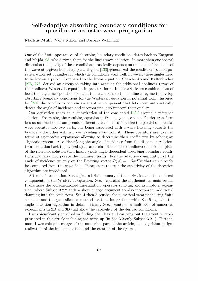
Self-adaptive absorbing boundary conditions forquasilinear acoustic wave propagation

Markus Muhr, Vanja Nikolić and Barbara Wohlmuth

One of the first appearances of absorbing boundary conditions dates back to Engquistand Majda [95] who derived them for the linear wave equation. In more than one spatialdimension the quality of these conditions drastically depends on the angle of incidence ofthe wave at a given boundary part. Higdon [133] generalized the conditions to incorpo-rate a whole set of angles for which the conditions work well, however, these angles needto be known a priori. Compared to the linear equation, Shevchenko and Kaltenbacher[275, 276] derived an extension taking into account the additional nonlinear terms ofthe nonlinear Westervelt equation in pressure form. In this article we combine ideas ofboth the angle incorporation side and the extensions to the nonlinear regime to developabsorbing boundary conditions for the Westervelt equation in potential form. Inspiredby [274] the conditions contain an adaptive component that lets them automaticallydetect the angle of incidence and incorporates it to improve their quality.Our derivation relies on a linearization of the considered PDE around a reference

solution. Expressing the resulting equation in frequency space via a Fourier-transformlets us use methods from pseudo-differential calculus to factorize the partial differentialwave operator into two parts, one being associated with a wave traveling towards theboundary the other with a wave traveling away from it. These operators are given interms of asymptotic expansions allowing to determine their coefficients by solving analgebraic system. Also identifying the angle of incidence from the dispersion relation,transformation back to physical space and reinsertion of the (nonlinear) solution in placeof the reference solution then finally yields angle dependent absorbing boundary condi-tions that also incorporate the nonlinear terms. For the adaptive computation of theangle of incidence we rely on the Poynting vector P (ψ) = −∂tψ∇ψ that can directlybe computed from the wave field. Parameters to steer the sensitivity of the detectionalgorithm are introduced.After the introduction, Sec. 2 gives a brief summary of the derivation and the different

components of the Westervelt equation. Sec. 3 contains the mathematical main result.It discusses the aforementioned linearization, operator splitting and asymptotic expan-sion, where Subsec. 3.2.2 adds a short energy argument to also incorporate additionaldamping into the conditions. Sec. 4 then discusses the numerical treatment using finiteelements and the generalized-α method for time integration, while Sec. 5 explains theangle detection algorithm in detail. Finally Sec. 6 contains a multitude of numericalexperiments in 2D and 3D that show the capability of the derived conditions.I was significantly involved in finding the ideas and carrying out the scientific work

presented in this article including the write-up (in Sec. 3.2 only Subsec. 3.2.1). Further-more I was solely in charge of the numerical part of the article, i.e. algorithm design,realization of the implementation and the creation of the figures.

67

Permission to include:

Muhr, Markus, Vanja Nikolić, and Barbara WohlmuthSelf-adaptive absorbing boundary conditions for quasilinear acoustic wavepropagation.Journal of Computational Physics 388 (2019): 279-299.

68

The above pages are copies from the webpagehttps://www.elsevier.com/about/policies/copyright

Date: 03.12.2019

The above pages are copies from the webpagehttps://s100.copyright.com/AppDispatchServlet#formTop

with input data:https://s100.copyright.com/AppDispatchServlet?translating=No&

rlPaymentProfileId=0&passThroughTarget=aboutyourwork-select&isMyAccount=

false&convertibleP=%3C%25%3Dconvertible%25%3E&orderCurrencyCode=EUR&

currentTargetPage=quickprice&myaccountlogin=true&publication=0021-9991&

circulationRange=15&insideApp=true&defaultBillingType=Credit+Card&

isCancelPressed=false&currentFooterPage=%2FApp%2FIncludes%2FFooter.jsp&

publicationID=12613&popBackPage=&doCalc=true&jsonScriptName=

&TermsAndConditions=&subPublisherID=-5555&buttonClicked=continue&

currentBodyPage=%2FApp%2FQuickPrice.jsp&orderBeanReset=false&format=both+

print+and+electronic&ignoreErrors=false&typeOfUseID=54&authorIndicator=Yes&

linkClicked=unknown&timeStamp=1575450429212&offerIDValue=542&portionUsed=

full+article&publisherID=70&install=&publisherName=ELS&loggedIn=false&

orderThreadID=-5144448019828798206&rightID=1&grantDenyCheckIgnoreErrors=

false&previousTargetPage=quickprice&requestToken=LAEVZ6C5oUFgz7PlJkJ7PAzz&

currentTargetPageID=6134707&targetPage=inflowlogin&currentHeaderPage=

%2FApp%2FIncludes%2FHeader.jsp&

Date: 09.12.2019

Journal of Computational Physics 388 (2019) 279–299

Contents lists available at ScienceDirect

Journal of Computational Physics

www.elsevier.com/locate/jcp

Self-adaptive absorbing boundary conditions for quasilinear

acoustic wave propagation

Markus Muhr ∗, Vanja Nikolic, Barbara Wohlmuth

Technical University of Munich, Department of Mathematics, Chair of Numerical Mathematics, Boltzmannstraße 3, 85748 Garching, Germany

a r t i c l e i n f o a b s t r a c t

Article history:Received 30 November 2018Received in revised form 18 March 2019Accepted 18 March 2019Available online 21 March 2019

Keywords:Absorbing conditionsNonlinear acousticsWestervelt’s equation

We propose a self-adaptive absorbing technique for quasilinear ultrasound waves in two-and three-dimensional computational domains. As a model for the nonlinear ultrasound propagation in thermoviscous fluids, we employ Westervelt’s wave equation solved for the acoustic velocity potential. The angle of incidence of the wave is computed based on the information provided by the wave-field gradient which is readily available in the finite element framework. The absorbing boundary conditions are then updated with the angle values in real time. Numerical experiments illustrate the accuracy and efficiency of the proposed method.

© 2019 Elsevier Inc. All rights reserved.

1. Introduction

Accurate simulation of nonlinear ultrasound offers a path to a better quality of many procedures in industry and medicine, from non-destructive detection of material damages [1–3] to non-invasive treatments of medical disorders [4–8]. When studying such procedures, there is always a region of interest: a kidney stone that will be disintegrated or a prop-agating fatigue crack in a component of an aircraft. The large physical space then often has to be truncated for numerical simulations. To accurately simulate ultrasound, we have to avoid spurious reflections of the wave at the boundary of the truncated domain.

Absorbing boundary conditions provide a simple and effective way of dealing with unwanted reflections. They were introduced by B. Engquist and E. Majda in their seminal work [9]. Since then many approaches have been developed for the non-reflecting boundary conditions; we refer the reader to the review papers [10,11] and the references given therein. In spite of such comprehensive research in this area, only a small portion of the results focus on nonlinear models.

A class of semilinear wave equations and nonlinear Schrödinger equations was investigated in [12,13]. Results for non-linear hyperbolic systems of the form ut + A(u)ux = 0 were obtained in [14]. An approach based on the operator splitting method was used in [15] to derive absorbing conditions for a semilinear wave equation of the form utt − a2u = f (u). In [16,17], nonlinear ultrasound propagation was investigated in this context for the first time, and absorbing conditions were developed for the Westervelt equation in the pressure form.

Another commonly used approach for avoiding spurious reflections is the Perfectly Matched Layer (PML) technique. Developed by J.-P. Bérenger in [18], this method introduces an artificial absorbing layer around the computational domain. Linear acoustic wave equations have been extensively studied in this context; see, for example, [19–23].

* Corresponding author.E-mail addresses: muhr@ma.tum.de (M. Muhr), vanja.nikolic@ma.tum.de (V. Nikolic), wohlmuth@ma.tum.de (B. Wohlmuth).

https://doi.org/10.1016/j.jcp.2019.03.0250021-9991/© 2019 Elsevier Inc. All rights reserved.

280 M. Muhr et al. / Journal of Computational Physics 388 (2019) 279–299

The main downside of absorbing conditions is that they are sensitive to the angle of incidence of the wave. As a rule of thumb, they perform bad if the range of incidence angles is large. The information on the incidence angles can be included in the conditions to tackle this issue; we refer to the work in [24–26]. However, these angles are not a priori known in a realistic computational setting. The idea behind the self-adaptive technique is to compute the local wave vector and then update the absorbing conditions with the angle information in real time. This approach was applied in [27] to the Schrödinger-type equations, where the wave number was computed via the Gabor transform. In [28], the linear wave equation was investigated in this context. It was proposed to divide the absorbing boundary into segments and compute the local incidence angle by employing the Fourier transformation only in the vicinity of the boundary. The self-adaptive approach to absorption can also be found in earlier works on acoustic scattering [29,30].

The goal of our work is to develop an efficient self-adaptive absorbing technique for nonlinear ultrasound propagation. As a model equation, we employ a classical quasilinear acoustic model - Westervelt’s equation. We first extend the results from [16,17] by considering the potential form of Westervelt’s equation and the non-zero angle of incidence θ . In addition, we derive the absorbing conditions for two- and three-dimensional computational domains. The derivation relies on choos-ing an appropriate linearization of the equation around a reference solution. The absorbing conditions are then formally derived for this linearization, after which we bring back the nonlinear term.

To obtain the angle θ in practice, we develop a self-adaptive method that locally computes the incidence angle and updates the absorbing conditions on the fly. Unlike the self-adaptive approach taken in [28], we base the local angle com-putation on the gradient of the wave field. Computation of the local propagation direction in isotropic media based on the information provided by the wave-field gradient has been studied in [31–36]. This approach is particularly suitable for our finite-element framework since the gradient information is already available at every time step in our simulations. The use of the field gradient information in the absorbing conditions has been already investigated for the Helmholtz equation in [37]. There it was proposed to replace the normal derivatives that appear in the absorbing conditions by the derivatives in the direction of the wave propagation. In the linear regime, our approach can be understood as an extension of the gradient method in [37] for a time-dependent wave model.

We organize the rest of the paper as follows. We begin in Section 2 by introducing the model and setting the problem. Section 3 contains the derivation of absorbing conditions for a given angle of incidence of the wave. In Section 4, we present the numerical scheme for solving the initial-boundary value problem for the Westervelt equation. Section 5 describes the computation of the local incidence angle via the information provided by the wave-field gradient. Finally, in Section 6, we present numerical experiments which illustrate the accuracy of the proposed adaptive boundary conditions.

2. Modeling and problem setting

The weakly nonlinear models in thermoviscous acoustics that are commonly used are obtained as an approximation of the compressible Navier-Stokes system. We here briefly reflect upon the derivation, which will give us a better understanding of the often-employed Westervelt equation. Mathematically rigorous justification of the classical acoustic models can be found in [38]. For a detailed insight into the acoustic field theory, we refer to [39–41].

Propagation of waves can be described by the time, the density , the pressure u and the velocity v, decomposed into their ambient value and the acoustic perturbation

= 0 + ,

u = u0 + u,

v = v0 + v;see [41]. We call the acoustic density, u the acoustic pressure, and v the acoustic particle velocity. The equations governing the wave propagation are then given by

• the equation of momentum conservation

(0 + )vt + 0

2∇(v · v) + ∇u =

(4νV

3+ ηV

)v,

• the equation of mass conservation

t + 0∇ · v = −∇ · v − v · ∇,

• the pressure-density relation

= 1

c2u − 1

0c4

B

2Au2 − κ

0c4

(1

c

− 1

cu

)ut .

Above, ηV denotes the bulk viscosity and νV the shear viscosity. The constant κ stands for the adiabatic exponent, cu and c

denote the specific heat capacitance at constant pressure and constant volume, respectively. The parameter of nonlinearity B/A is an indicator of the nonlinearity of the medium. Finally, c denotes the speed of sound in the fluid.

M. Muhr et al. / Journal of Computational Physics 388 (2019) 279–299 281

This system of equations is approximated by one model, whereby every term of order two and higher in the acoustic Mach number is neglected. This approach results in⎧⎪⎨

⎪⎩1c2 utt − u − b

c2ut = 1

0c4

B

2Autt + 0

c2

∂2

∂t2(v · v),

0vt = −∇u,

(1)

where the so-called sound diffusivity b is given by

b = 1

0

(4νV

3+ ηV

)+ κ

0

(1

cV− 1

cu

).

The acoustic velocity potential ψ is then introduced to obtain a scalar equation; it is related to the acoustic pressure by

u ≈ 0ψt, (2)

and to the acoustic particle velocity by

v = −∇ψ. (3)

By expressing (1) in terms of ψ , integrating with respect to time and taking the resulting constant of integration to be zero, we arrive at the Kuznetsov equation

1

c2ψtt − ψ − b

c2ψt = B/A

c4ψtψtt + 2

c2∇ψ · ∇ψt; (4)

cf. [42]. If the cumulative nonlinear effects dominate the local ones in the sense of

2

c2∇ψ · ∇ψt ≈ 2

c4ψtψtt, (5)

a simplification of (4), known as the Westervelt equation [43], is obtained

1

c2ψtt − ψ − δψt = k

c2ψtψtt . (6)

Above we have introduced the notation

δ = b

c2, k = 1

c2(B/A + 2). (7)

After numerically solving (6), the pressure field can be obtained in a post-processing step via the relation (2). We mention as well that the Westervelt equation in the pressure form is given by

1

c2utt − u − δut = k

c2(uutt + u2

t ). (8)

Equation (8) can be obtained from (1) by employing the approximation (5) which in terms of the velocity and pressure reads as

0(v · v)t ≈ 1

0c2(u2)t .

3. Absorbing conditions for the Westervelt equation

We consider the Westervelt equation (6) on a three-dimensional spatial domain = (x, y, z) : x < 0, y, z ∈ R. We restrict ourselves in the problem description to the case of positive constant coefficients c, b, and k.

3.1. Linearization of the Westervelt equation

Following the approach from [16] where equation (8) was considered, we derive absorbing conditions for the Westervelt equation in the potential form (6) by first transforming it into a linear equation, deriving the non-reflecting conditions for this linear model, and then “plugging” back in the nonlinear term.

It is clear that the linearization of the equation plays a crucial role in deriving the absorbing conditions. A possible linearization of the Westervelt equation around a reference solution ψ ref is given by

1

c2ψtt − ψ − δψt = k

c2β(x, y, z, t)ψtt, (9)

282 M. Muhr et al. / Journal of Computational Physics 388 (2019) 279–299

where β = ψ reft . We note that, unlike in the derivation of the Westervelt equation in Section 2, here we do not split ψ into

a background and oscillatory part, instead we assume ψ ref to be a solution of the equation. This linearization is analogous to the one employed in [16] for the equation in the pressure formulation (8).

We propose an alternative linearization. Note that the right-hand side of the Westervelt equation (6) can be rewritten as 1

2

k

c2(ψ2

t )t . We linearize the term ψ2t as ψ ref

t ψt and study the following equation

1

c2ψtt − ψ − δψt = 1

2

k

c2(β(x, y, z, t)ψt)t, (10)

where again β = ψ reft . The absorbing boundary conditions based on linearizations (9) and (10) are numerically compared in

Section 6.We first derive absorbing conditions for the linear equation (10) and a given angle of incidence. After obtaining the

conditions for such a model, the coefficient β is set back to ψt to obtain nonlinear conditions.We remark that the linearization via Taylor expansion around a reference solution ψ ref is not considered here since it

would introduce the term ψ reft ψ ref

tt into the linearized equation; we refer to a similar discussion in [16].

3.2. Derivation of absorbing conditions for the angle of incidence θ

We study here the derivation of the absorbing conditions for the linearization (10); equation (9) can be treated analo-gously. To derive the conditions, we could use the frozen coefficient approach which first transforms the variable coefficient equation into its constant-coefficient counterpart by “freezing” its coefficients at a given point before employing the Fourier transform in the (y, z, t) coordinates; cf. [9, Section 1]. Although the main focus of the present work is the derivation of the zero-order (adaptive) absorbing conditions, we still follow the approach based on the pseudo-differential calculus since it allows to arrive at a general system for determining the correcting terms beyond order zero in the absorbing conditions; see system (19) below.

We first rewrite the linearized equation (10) in the operator form as

Pu = 0, (11)

where the operator P is given by

P =(

1

c2− 1

2

k

c2β(x, y, z, t)

)∂2

t − ∂2x − ∂2

y − ∂2z − δ∂2

x ∂t − δ∂2y∂t − δ∂2

z ∂t − 1

2

k

c2βt(x, y, z, t)∂t . (12)

At this point we also introduce

α0(x, y, z, t) =√

1

c2− 1

2

k

c2β(x, y, z, t),

α1(x, y, z, t) = 1

2

k

c2βt(x, y, z, t).

(13)

Note that the well-posedness results for the Westervelt equation rely on the fact that the factor 1c2 (1 − kψt) next to the

second time derivative remains positive; see [44–46]. Therefore, it is reasonable to assume that the term under the square root in (13) is positive for sufficiently small data. We note that we proceed heuristically since the rigorous justification of the derivations given below would also require C∞ regularity of α0 and α1 which is not proven here.

Absorbing boundary conditions for (11) will be derived by employing the pseudo-differential calculus and factorization of the operator P according to L. Nirenberg’s procedure [47, Chapter II]. We briefly summarize the procedure here for the convenience of the reader. A detailed account on the pseudo-differential operators can be found in [48,47,49].

Definition 1. [49,50] Let the set Sm , where m ∈ R, be defined as the set of all functions q(t, τ ) ∈ C∞(Rd ×Rd) such that for any two multi-indices k and l, there is a positive constant Ckl depending only on k and l, such that

|∂kt ∂ l

τ q(t, τ )| ≤ Ckl(1 + |τ |)m−|l|, t, τ ∈ Rd.

Sm is called the space of symbols of order m. We set S−∞ = ∩m∈RSm .

Definition 2. [49, Definition 5.2] Let q be a symbol. The pseudo-differential operator Q associated to q is defined by

(Qϕ)(t) = (2π)−d/2∫Rd

eit·τ q(t, τ )Fϕ(τ )dτ ,

where ϕ is a function from the Schwartz space, and F denotes the Fourier transform.

M. Muhr et al. / Journal of Computational Physics 388 (2019) 279–299 283

3.2.1. Propagation without lossesFollowing the approach in [16], we first derive the absorbing conditions with the assumption that δ = 0. This assumption

facilitates the derivation of the conditions based on the pseudo-differential factorization. The δ-term will be included as a post-processing step based on energy arguments.

The derivation of the conditions relies on the fact that the operator P can be factorized into the form

P = − (∂x − A

(x, y, z, t, ∂y, ∂z, ∂t

)) (∂x − B

(x, y, z, t, ∂y, ∂z, ∂t

)) + R(x, y, z, t, ∂y, ∂z, ∂t

) ; (14)

see [47, Lemma 1]. In (14), the operators A and B are pseudo-differential operators with the symbols a(x, y, z, t, η, ζ, τ )

and b(x, y, z, t, η, ζ, τ ), respectively, from the space S1. The conditions on A that we will develop will have the effect of associating A with waves that travel out of the computational domain. The pseudo-differential operator R is a smoothing operator with the full symbol r(x, y, z, t, η, ζ, τ ) that belongs to S−∞ .

The symbols a and b formally admit asymptotic expansions

a(x, y, z, t, η, ζ, τ ) ∼∑j≥0

a1− j(x, y, z, t, η, ζ, τ ),

b(x, y, z, t, η, ζ, τ ) ∼∑j≥0

b1− j(x, y, z, t, η, ζ, τ ),

where a1− j and b1− j denote homogeneous functions of degree 1 − j with respect to τ ; see [49, Theorem 5.10]. We note that the symbol a(x, y, z, t, η, ζ, τ )b(x, y, z, t, η, ζ, τ ) of the product of A and B has an asymptotic expansion as well

a(x, y, z, t, η, ζ, τ )b(x, y, z, t, η, ζ, τ ) ∼∑j≥0,

k+l+n= j,k,l,n≥0

(−1)n

n! ∂nτ a1−l(x, y, z, t, η, ζ, τ )∂n

t b1−k(x, y, z, t, η, ζ, τ );

see [49, Theorem 7.1].According to [51, Theorems 1 and 2], absorbing boundary conditions on the boundary x = 0 are given in the form

(∂x − A

(x, y, z, t, ∂y, ∂z, ∂t

))ψ

∣∣∣x=0

= 0.

Since the symbol a of A has an infinite expansion, in numerical simulations this expansion is truncated after a certain number of terms. Absorbing conditions of order k ∈N0 are then on the symbolic level given by⎛

⎝∂x −k∑

j=0

a1− j(0, y, z, t, η, ζ, τ )

⎞⎠ψ

∣∣∣x=0

= 0. (15)

The higher-order absorbing conditions, although numerically more accurate, are also significantly more involved when it comes to implementation. We will compute the absorbing conditions of order zero for the given angle of incidence θ . Combined with the proposed self-adaptive technique, this approach allows to improve the accuracy of zero-order conditions, yet keeps them easy to implement.

We recall how the operator P was defined in (12), set δ = 0, and then develop factorization (14) to obtain

α20 ∂2

t − ∂2x − ∂2

y − ∂2z − α1∂t

= − ∂2x + (A + B)∂x + Bx − AB + R.

(16)

By employing the asymptotic expansion of the symbols a, b, and ab, equation (16) reduces on the symbolic level to

α20(iτ )2 − (iη)2 − (iζ )2 − α1(iτ )

∼=∑j≥0

(a1− j + b1− j)∂x +∑j≥0

∂xb1− j −∑j≥0,

k+l+n= j,k,l,n≥0

(−1)n

n! ∂nτ a1−l∂

nt b1−k. (17)

Above, we have denoted the dual variables to t , y, and z by τ , η, and ζ , with the correspondence ∂t ↔ iτ , ∂y ↔ iη, and ∂z ↔ iζ . Following the notation in [9], ∼= stands for “within a smooth error” because we have dropped R. We note that the operator R can only be controlled in terms of its smoothness. However, its action on the solution is expected to be negligible for high frequencies that are present in ultrasound waves.

284 M. Muhr et al. / Journal of Computational Physics 388 (2019) 279–299

Fig. 1. Illustration of the interplay between the wave vector k, outward normal vector n, and the angle of incidence θ .

To determine a1 and b1, we equate the symbols with the same degree of homogeneity with respect to τ and get the system

a1 + b1 = 0

a1b1 = −(α20(iτ )2 − (iη)2 − (iζ )2),

(18)

assuming that α20τ

2 ∼= η2 + ζ 2. The system that determines the coefficients a1− j, b1− j j≥1 is then given by⎧⎪⎪⎪⎪⎨⎪⎪⎪⎪⎩

a1− j + b1− j = 0, j ≥ 1,

−α1(iτ )δ j1 = −∑j≥1,

k+l+n= j,k,l,n≥0

(−1)n

n! ∂nτ a1−l∂

nt b1−k + ∂xb1− j, (19)

where δ denotes the Kronecker delta. From (18), we find that

a1 = −√

α20(iτ )2 − (iη)2 − (iζ )2

and

b1 =√

α20(iτ )2 − (iη)2 − (iζ )2.

Note that the sign of a1 determines the propagation direction of the wave. To obtain the absorbing conditions for the given angle of incidence, we freeze the coefficient β in (12) by assuming that it is constant in space and time. The dispersion relation for (10) when β is constant is as follows

α20(iτ )2 − (iξ)2 − (iη)2 − (iζ )2 = 0. (20)

The wave vector is given by (ξ, η, ζ ). If we denote by θ ∈ [0, 90] the angle between the incident wave and the outer normal to the boundary, we have for τ > 0

sin θ =√

η2 + ζ 2√ξ2 + η2 + ζ 2

=√

η2 + ζ 2

α0τ;

see Fig. 1.Therefore, we can express a1 as

a1 = − α0(iτ )

√1 − η2 + ζ 2

α20τ

2= −α0(iτ ) cos θ.

According to (15), the absorbing conditions of order zero are then given by

∂ψ

∂n= −α0 ψt cos θ. (21)

M. Muhr et al. / Journal of Computational Physics 388 (2019) 279–299 285

We mention that for a variable coefficient problem with jumps outside the computational domain, it is not possible to build

an exact ABC based on local computations. After returning to β = ψt and α0 =√

1

c2 − 1

2

k

c2 ψt , we obtain the absorbing boundary conditions for the inviscid Westervelt equation in the potential formulation for a given angle of incidence θ :

c∂ψ

∂n+

√1 − k

2ψt ψt cos θ = 0. (22)

3.2.2. Propagation with lossesWe next want to incorporate the b term into the conditions. This was not possible before since we needed b = 0 to

make use of the pseudo-differential factorization and the dispersion relation (20). Instead, we employ a reasoning based on an energy argument.

To this end, we test the linearized equation (10) with ψt , integrate over space and (0, t), where t ≤ T , and integrate by parts with respect to time, to arrive at the following identity:

E0[ψ](t) + δ

t∫0

‖∇ψt‖2L2()

ds

= E0[ψ](0) +t∫

0

∫

(12 (α2

0)t + α1

)ψ2

t dxds +t∫

0

∫∂

(∂ψ

∂n+ δ

∂ψt

∂n

)ψt dxds,

(23)

where the energy is given by

E0[ψ](t) = 1

2

(‖α0(t)ψt(t)‖2

L2()+ ‖∇ψ(t)‖2

L2()

).

This identity suggests to modify the conditions (21) to include the sound diffusivity as follows

∂ψ

∂n+ δ

∂ψt

∂n= −α0 ψt cos θ on abc. (24)

These conditions facilitate the extraction of energy through the boundary since (23) becomes

E0[ψ](t) + δ

t∫0

‖∇ψt‖2L2()

ds +t∫

0

∥∥∥√α0 cos θ ψt

∥∥∥2

L2(∂)ds

= E0[ψ](0) +t∫

0

∫

( 12 (α2

0)t + α1)ψ2t dxds,

(25)

from which by employing Gronwall’s inequality it follows that

E0[ψ](t) + δ

t∫0

‖∇ψt‖2L2()

ds +t∫

0

∥∥∥√α0 cos θ ψt

∥∥∥2

L2(∂)ds ≤ C(T )E0[ψ](0),

provided 12 (α2

0)t + α1 ∈ L∞(0, T ; L∞()).

We therefore adopt conditions (24). After returning to β = ψt and α0 =√

1

c2− 1

2

k

c2ψt in (24) and recalling that δ = b/c2,

we obtain the nonlinear conditions

c2 ∂ψ

∂n+ b

∂ψt

∂n= − c

√1 − k

2ψt ψt cos θ on abc. (26)

We note that in realistic settings the sound diffusivity b in fluids is small; see, e.g., [41]. It is also known that the presence of a large b damping in the model would imply a parabolic instead of a wave-like behavior of the equation resulting in an exponential decay of the energy; cf. [44, Theorem 3.3].

Setting k to zero in (26) corresponds to conditions for a linear, strongly damped wave equation. If in addition b = 0, we end up with the standard linear absorbing conditions for the angle θ

c∂ψ

∂n+ ψt cos θ = 0 on abc; (27)

see [24,26].

286 M. Muhr et al. / Journal of Computational Physics 388 (2019) 279–299

Remark 1 (One- and two-dimensional domains). In a one-dimensional setting, system (18) for determining the symbols a1 and b1 simplifies to

a1 + b1 = 0

a1b1 = −α20(iτ )2.

In a two-dimensional setting, system (18) simplifies toa1 + b1 = 0

a1b1 = −(α20(iτ )2 − (iη)2).

It is then straightforward to show that conditions (26) hold in 1D and 2D as well, where in 1D the angle θ can be interpreted as being set to θ = 0 .

Remark 2 (A different linearization). Employing linearization (9) would result in the following absorbing conditions

c2 ∂ψ

∂n+ b

∂ψt

∂n= − c

√1 − kψt ψt cos θ on abc. (28)

The performance of conditions (26) and (28) is compared in Section 6, where the proposed conditions (26) significantly outperform (28).

Remark 3. In our experiments, we employ the gradient information to compute the angle of incidence θ via

cos θ = |∇ψ · n|√ψ2

x + ψ2y + ψ2

z

on abc,

assuming that ∇ψ = 0 on the absorbing boundary. The linear conditions (27) for the angle θ are then equivalent to

c|∇ψ | + ψt = 0 on abc. (29)

Therefore, in the linear regime, conditions (29) can be seen as the extension of the absorbing conditions proposed in [37]for the Helmholtz equation to the linear time-dependent wave model.

4. Numerical treatment

After deriving the absorbing boundary conditions for the potential form of the Westervelt equation (6), we next focus on the numerical schemes used in simulations. We begin by formulating the initial-boundary value problem that has to be solved.

4.1. The initial-boundary value problem for the Westervelt equation

We consider the following problem for the Westervelt equation:⎧⎪⎪⎪⎪⎪⎪⎪⎪⎪⎪⎪⎪⎨⎪⎪⎪⎪⎪⎪⎪⎪⎪⎪⎪⎪⎩

ψtt − c2ψ − bψt = 1

c2(B/A + 2)ψtψtt in × (0, T ),

ψ = g on exc × (0, T ),

c∂ψ

∂n+ b

c

∂ψt

∂n= −√

1 − σkψt ψt cos θ(ψ) on abc × (0, T ),

∂ψ

∂n= 0 on N × (0, T ),

ψ = ψt = 0 in × 0.

(30)

The wave source is given in the form of inhomogeneous Dirichlet conditions on the excitation part of the domain boundary exc ⊂ ∂. In our numerical tests, the excitation signal is always taken to be a modulated sine wave, that is growing over time until its maximal amplitude is reached, i.e.,

g(t) =

( f 2/4)t2 A sin(ωt), t < 2/ f ,

A sin(ωt), t ≥ 2/ f ,(31)

where f denotes the frequency, ω = 2π f the angular frequency, and A the maximal amplitude of the signal.

M. Muhr et al. / Journal of Computational Physics 388 (2019) 279–299 287

We have introduced the parameter σ within the square root of the absorbing conditions in (30). In this way, we gen-eralized in one formula all the absorbing conditions that we want to compare. Indeed, setting σ = 0 yields the adaptive absorbing conditions for the linear strongly damped wave equation

c∂ψ

∂n+ b

c

∂ψt

∂n= −ψt cos θ(ψ), (32)

which we denote from now on in experiments by “ABC0W adaptive”. In case also θ = 0 everywhere, we denote them just by

ABC0W. Setting σ = 1/2 recovers our new nonlinear adaptive conditions, denoted by “ABC1/2

W adaptive”. If the angle is always set to zero, we denote them just by ABC1/2

W . Finally, σ = 1 leads to conditions based on the second linearization (9), which are denoted in the experiments by “ABC1

W adaptive” and ABC1W.

We start from the weak form of the problem (30). We are looking for a solution in

ψ ∈ C1([0, T ]; H2()) ∩ C2([0, T ]; H1()) | ψ = g on exc × (0, T )such that∫

((1 − kψt)ψtt v + c2∇ψ · ∇v + b∇ψt · ∇v)d +∫

abc

c√

1 − σkψt ψt cos θ(ψ) v dS = 0

for all test functions in v ∈ H1() | v = 0 on exc × (0, T ) a.e. in time, with (ψ, ψt)|t=0 = (0, 0). We assume that the prob-lem (30) is well-posed, although the rigorous proof is beyond the scope of the current work. Results on the well-posedness of the Westervelt equation in the pressure form with nonlinear absorbing conditions for the angle of incidence θ = 0 can be found in [17,52].

4.2. Finite element discretization and time integration

We follow the standard discretization methods for nonlinear acoustics based on finite elements [41,53–57]. The finite element method is employed in space with lowest order conforming elements on simplicial meshes.

The mass M, stiffness K, and damping matrix C as well as the nonlinearity tensor T are assembled in the usual manner; see [41,56]. By dividing the set of degrees of freedom into the set of Dirichlet degrees D and the set of interior degrees I, the semi-discrete problem reads as follows⎧⎪⎪⎨

⎪⎪⎩MI,Iψ I

+ KI,Iψ I+ CI,Iψ I

− T I,I,I[ψ I, ψ

I, ·] − T I,D,I[ψ I

, ψD, ·]

−T D,I,I[ψD, ψ

I, ·] + AI(ψ, ψ, θ(ψ)) = F (t) in (0, T ),

ψ = ψ = 0 at t = 0.

(33)

The right-hand side of the equation is given by

F (t) = −MI,DψD

− KI,DψD

− CI,DψD

+ T D,D,I[ψD, ψ

D, ·].

The underlined quantities ψ, ψ , and ψ denote the coefficient vectors of ψ, ψt , and ψtt resulting from the spatial finite element discretization. The compact notation with index sets D and I is used to extract the respective rows and columns of matrices and vectors that belong to Dirichlet and interior degrees of freedom.

The absorbing boundary vector A is formally given by

A(ψt, θ(ψ)) = (Ai(ψt, θ(ψ)))i∈DOF(abc),

Ai(ψt, θ(ψ)) =∫

abc

c√

1 − σkψt ψt cos θ(ψ) Ni dS. (34)

Above, Ni stands for the finite element ansatz function of the i-th global degree of freedom, while DOF(abc) is the set of degrees of freedom belonging to the absorbing boundary.

The nonlinearity tensor T is used to resolve the nonlinear bulk term in the weak formulation in a fixed-point iteration. The same also holds for the absorbing boundary vector which is iteratively updated with the current values of ψt , ψtt as well as updates for the angle θ .

The system (33) is a nonlinear system of ordinary differential equations of second order with |I| components. It remains to solve it by using a suitable time integrator. Following [56], we employ the Generalized-α scheme in combination with the Newmark relations for time integration. Values of the Generalized-α parameters (αm, α f ) and the Newmark parameters

288 M. Muhr et al. / Journal of Computational Physics 388 (2019) 279–299

Table 1Time-stepping parameters.

parameter value

Newmark-parameters βnm 4/9γnm 5/6

Generalized-α parameters αm 0α f 1/3

Nonlinear iteration parameters TOL 10−6

κmax 100

(βnm, γnm) that are used in experiments are chosen according to the stability and accuracy criteria stated in [58]:

αm = 2ρ∞ − 1

1 + ρ∞, α f = ρ∞

1 + ρ∞, βnm = 1

(1 + ρ∞)2, γnm = 1

2

3 − ρ∞1 + ρ∞

where we take ρ∞ = 1/2; see also Table 1 for the resulting values.In comparison to the numerical solvers proposed in [53,56], a new aspect of our method is the computation of the angle

of incidence θ(ψ). The angle is computed once in every time step before the first assembly of the absorbing boundary vector. Details on how we compute the angle can be found in Section 5.

5. Computation of the angle of incidence

It remains to see how we can compute the angle of incidence θ that the local wave vector encloses with the outward normal to the absorbing boundary at a given point on abc. To reduce the computational cost, we compute the angle θ once per time step and do not update it within the nonlinear fixed-point iteration.

According to [33,35], the Poynting vector P(ψ) of a wave field ψ can be used to compute its local propagation direction. The vector P(ψ) is given by

P(ψ) = −∂ψ

∂t∇ψ. (35)

Since neither the sign nor the norm of the propagation vector plays a role when computing the incidence angle, we restrict ourselves to the spatial gradient alone to determine the main propagation direction of the wave. Such an approach was also taken in [31,34,36] for wave fields in an isotropic medium. In our case, this method of computing the local propagation direction works especially well since, although globally discontinuous, the element-wise gradient information is readily available at every time step in the finite element framework. We also refer to [32] for a further discussion on the use of the Poynting vector in angle decomposition methods.

We conduct experiments with zero initial data and inhomogeneous Dirichlet conditions on part of the boundary, and so most of the potential field is at rest at the beginning of the simulation. However, numerical noise of low magnitude can be present at the absorbing boundary before the wave reaches it. Such behavior could be accounted to weak ill-posedness; see [59]. To tackle this issue, we implement a switch. When going over all elements adjacent to the absorbing boundary, we only compute the element-wise angle of incidence once the local wave amplitude (in terms of absolute value of the elements degrees of freedom) exceeds a certain percentage p1 of a reference value; see Algorithm 1, line 3. We take the reference value to be the source amplitude of the wave. In the case that the source amplitude is not known a priori, an alternative would be to compute the maximum field amplitude in the interior of the domain and take this as a reference value. As long as the criterion is not matched, the local angle of incidence is set to 0; see Algorithm 1, line 14. We note that a similar approach was taken in [28]. In all our numerical experiments, we set p1 = 0.1.

Algorithm 1 summarizes our method of computing the incidence angle. Within the algorithm, indices in the exponent indicate the time step.

Note that even once the local amplitude of the wave at a given element is large enough for the angle computation to start, unreliable angle values can be computed at points where a local wave maximum or minimum hits the boundary since the gradient is close to zero. As a remedy, we propose that gradients with the Euclidean norm below some threshold should not influence the angle of incidence. Whenever such a small gradient appears, we use the angle of the last time step; see Algorithm 1, line 9. We employ a percentage p2 of a reference value for the threshold.

As the reference value we take the local gradient history of the given element and pick the norm-wise maximum over the past time steps; see Algorithm 1, line 8. We compute a new angle of incidence only in cases where the threshold is surpassed, i.e., when the local gradient is sufficiently large; cf. Algorithm 1, line 11. To also reduce the oscillations with respect to time in the angle distribution, in all experiments we choose a relatively high threshold of p2 = 0.5.

Together with the previously introduced switch, the above approach allows to steer the sensitivity of the angle computa-tion algorithm by adapting the parameters p1 and p2. If these parameters are close to 1, the angle is only computed for very high amplitudes and local gradients, while for most other parts of the boundary the angle remains zero. On the other hand, small values of p1 and p2 would lead to highly sensitive angles that react to even small perturbations in the wave field.

M. Muhr et al. / Journal of Computational Physics 388 (2019) 279–299 289

Algorithm 1: Angle-computation algorithmInitialization:

1 Formally set |∇ψ(−1)

el | = ∞ and θ0el = 0 for all elements el

In time step n = 1,2, ... do

2 for el ∈ elements : element has an edge/face on the absorbing boundary3 if max|ψn

i | : dofi belongs to el > p1 · A then4 enable angle computation for el5 end6 if angle computation is enabled for el then7 Evaluate ∇ψ(x, tn−1) within el → save as ∇ψn−1

el

8 if |∇ψn−1el | ≤ p2 max

k<n−1|∇ψk

el| then

9 set θnel = θn−1

el10 else

11 compute θnel = arccos

( |〈∇ψn−1el , nel〉|

|∇ψn−1el |

)

12 end13 else14 set θn

el = 015 end16 end

Fig. 2. Computational domains used in simulations. (Top left) Channel with an inclined absorbing boundary, (Top right) Octant of a “plate with hole” geometry, (Bottom left) Geometry of a focusing transducer, (Bottom right) Geometry with multiple sources and wave superposition.

6. Numerical results

We proceed with numerical simulations where we put our self-adaptive technique to the test. Computational domains used in numerical experiments are sketched in Fig. 2. The dashed lines symbolize the boundaries of the reference domain ref where we compute the reference solution ψ ref. The reference solution is always first computed on ref , then restricted to the actual domain , and compared with the potential field obtained on by employing the absorbing conditions.

We mention again that in all numerical simulations conforming finite elements of lowest order on simplicial meshes are used. Geometry and mesh are generated by using the Gmsh software package [60].

290 M. Muhr et al. / Journal of Computational Physics 388 (2019) 279–299

Fig. 3. Time snapshots of the potential field.

Fig. 4. Inclined plane boundary: Relative L2() error of the potential ψ(t) over the simulation time with θ = 20 . (Left) Nonlinear vs. linear conditions with and without adaptivity, (Right) Performance of adaptive conditions with numerically computed vs. the exact incidence angle θ . (For interpretation of the colors in the figure(s), the reader is referred to the web version of this article.)

6.1. Domain with an inclined absorbing boundary

In our first experiment, we consider a two-dimensional channel geometry, where the upper (absorbing) boundary abc is tilted by a given angle of θ ; see Fig. 2. The waves originate from the excitation boundary exc at the bottom of the rectangle and travel straight upwards. We impose homogeneous Neumann boundary conditions on the sides of the domain. The wave vector k in this setting points straight upwards. Therefore, the angle that the wave vector and the outward normal n of at abc enclose is exactly θ for the absorbing boundary.

We compute the reference solution ψ ref on a larger domain without the absorbing boundary and then conduct a simu-lation on . To get an impression on how the wave propagates in the present setting, Fig. 3 shows the potential field ψ at different time snapshots. Material parameters were chosen to be the ones of water, i.e.

c = 1500 m/s, b = 6 · 10−9 m2/s, ρ = 1000 kg/m3, B/A = 5;see [41, Chapter 5], while the excitation (31) has an amplitude of A = 0.01 m2/s2 and a frequency of 210 kHz. The experi-ment was conducted for two different angles

θ ∈ 20,50.For spatial discretization, we take 13045 (20 case) and 13046 (50 case) degrees of freedom in space for the channel width of 0.02 m and channel length (in the middle) of 0.03 m. In time, 9800 time steps were taken to cover the interval from t0 = 0 s until T = 9.45 · 10−5 s.

The error plots are given in Fig. 4. We observe that the conditions that do not take the angle of incidence into consid-eration significantly deteriorate when the angle increases. For the angle of incidence θ = 50 , the maximal relative error is more than 20% for the linear conditions and around 17% for the nonlinear conditions with the fixed angle θ = 0 . In comparison, the self-adaptive technique when combined with the nonlinear conditions (26) allows for the error to remain around 1%. Note that linearization (10) and the resulting absorbing conditions (26) clearly outperform conditions (28). We,

M. Muhr et al. / Journal of Computational Physics 388 (2019) 279–299 291

Fig. 5. Inclined plane boundary: Relative L2() error of the potential ψ(t) over the simulation time with θ = 50 . (Left) Nonlinear vs. linear conditions with and without adaptivity, (Right) Performance of adaptive conditions with numerically computed vs. the exact incidence angle θ .

therefore, proceed in the following experiments with testing only (26) in combination with the self-adaptive technique. We also observe that the nonlinear conditions (26) that use an approximate angle computation via the gradient of the wave field perform similarly to the conditions that employ the exact angle.

It is also interesting to see how the errors are distributed over the domain , i.e., where they originate from and how far they spread. Fig. 6 shows the error fields |ψ(t) − ψ ref(t)| at different times for the ABC1/2

W conditions with and without adaptivity. The first snapshots were taken just as the first wave hits the absorbing boundary. In the subsequent snapshots, we can see how the erroneous reflections travel together with the wave across the absorbing boundary. It is evident that there are fewer reflections present when using the self-adaptive absorbing boundary conditions that take the local angle information into account.

6.2. Higher source frequency

So far our experiments have been conducted with the same source excitation. After varying the domain geometry via the angle θ , we investigate the influence of the source frequency on the quality of absorbing conditions. We now test with the excitation frequency

f = 250 kHz.

All the remaining parameters being the same as before. The domain again has the upper boundary tilted with the angle of 50 . Fig. 7 shows the error plots for the higher frequency. We observe that conditions ABC0

W asymptotically show the same poor results as conditions ABC0

W with self-adaptivity. Only our combination of nonlinear conditions with the self-adaptive technique (26) allows for the relative error to stay around 1%. By comparing Fig. 5 and Fig. 7, we also notice that the difference in the error between the nonlinear and the corresponding linear conditions increases with the frequency, emphasizing the need to employ nonlinear conditions for high-frequency nonlinear sound waves.

6.3. Plate with a hole

We previously tested the new absorbing boundary conditions in a domain where the angle of incidence was constant over the absorbing boundary. To show that both our approach of computing the angle of incidence of the wave as well as the nonlinear boundary conditions work in more realistic settings, we now consider the so-called “plate with a hole” domain. It consists of a square with a circular hole in the center. In our case, the excitation of the wave takes place at the boundary of the hole. By using symmetry, we reduce the simulation of the whole domain to half of one of its quarters; see Fig. 2.

An analytical expression for the angle of incidence is also available here which allows us to judge the quality of our angle approximation. If the origin is at the center of the circular hole and the square has sides of length a, the angle of incidence is given by

θ(x, y, t) = arccos

(a/2√

x2 + (a/2)2

). (36)

We set a = 0.08 in the experiments. The domain is resolved with 13820 degrees of freedom in space. For time discretization, we choose 8330 time steps with final time T = 8.0325 · 10−5 s.

Fig. 8 shows the angle of incidence computed by our approach at two different points in time and further illustrates our criterion on computing the incidence angle based on the amplitude of the wave on the boundary. Note that formula (36) assumes a reflection-free potential field so an exact match of our angle to the analytical angle distribution cannot

292 M. Muhr et al. / Journal of Computational Physics 388 (2019) 279–299

Fig. 6. Potential difference |ψ(t) − ψ ref(t)| plotted over time (Horizontal) for ABC1/2W (First row) without adaptivity and (Second row) with self-adaptive

angle.

Fig. 7. Inclined plane boundary: Relative L2() error of the potential ψ(t) for t ∈ [0, T ] with θ = 50 and higher source frequency. (Left) Nonlinear vs. linear conditions with and without adaptivity, (Right) Performance of adaptive conditions with numerically computed vs. the exact incidence angle θ .

Fig. 8. Computed versus exact angle of incidence θ . (Left) The angle is only computed on the parts of the absorbing boundary that the wave has reached.(Right) Angle computation towards the end of the simulation.

M. Muhr et al. / Journal of Computational Physics 388 (2019) 279–299 293

Fig. 9. Time snapshots of the pressure field u = ρψt .

Fig. 10. Pressure difference |u(t) − uref(t)| plotted over time (Horizontal) for ABC1/2W without (First row) and with (Second row) angle consideration.

Fig. 11. Plate with a hole: Relative L2() error of (Left) the potential ψ(t) and (Right) the pressure u(t) = ρψt (t) over the simulation time.

be expected. In fact, our method tries to compensate also for the waves that originate as spurious reflections from the absorbing boundary.

As in our last experiment, we proceed by showing the wave field at different time steps as well as the error comparison of different absorbing boundary conditions; see Fig. 9 and Fig. 11. This time we also compute them in terms of the acoustic pressure u = ρψt due to its practical importance. We also introduce here the relative errors in the L2(0, T ; L2()) norm, i.e.

eψ = ‖ψ − ψ ref‖L2(0,T ;L2())

‖ψ ref‖L2(0,T ;L2())

, eu = ‖u − uref‖L2(0,T ;L2())

‖uref‖L2(0,T ;L2())

.

In the present experiment, those errors amount to eψ = 1.82% and eu = 0.93% for the self-adaptive conditions and eψ = 5.41% and eu = 5.17% for the conditions without adaptivity, giving an overall improvement of 66.36% in the potential and 82.01% in the pressure.

Plots of the difference field |u(t) − uref(t)| at different times are given in Fig. 10. We observe that with the absorbing conditions that are not adaptive, the amplitude of the error increases over the width of the domain as the angle grows.

294 M. Muhr et al. / Journal of Computational Physics 388 (2019) 279–299

Fig. 12. Snapshots of the pressure field u = ρψt of a propagating, self-focusing wave.

Fig. 13. HIFU transducer in 2D: Relative L2() error of (Left) the potential ψ(t) and (Right) the pressure u(t) = ρψt (t) over the simulation time.

6.4. High-intensity focused ultrasound (HIFU)

We next simulate the potential field generated by a piezoelectric transducer. Such devices are made of small plates of a piezoelectric material that are aligned in an arc-shaped array pointing towards a common focal point [61,62]. When set into motion, those vibrating plates induce acoustic sound waves that propagate towards the focal point. As it travels, the wave is focused more and more the closer it comes to the focal point. This technique of generating high-pressure amplitudes at specific locations is used in medicine to treat kidney stones and certain types of cancer; see [4–8]. The pressure levels in the non-focal region are sufficiently low so that damage to the surrounding tissue is avoided.

For this experiment, the medium of propagation is again chosen to be water with the same physical parameters as before. The source frequency is again given by f = 210 kHz and the source amplitude by A = 0.02 m2/s2 which increases at the focal point due to focusing. As depicted in Fig. 2, the absorbing boundary here consists out of three line segments at the left, right and top. Time-snapshots of the transducer simulation can be seen in Fig. 12.

The computational domain was resolved with 13313 degrees of freedom, while for the time stepping 9800 steps and a final time of T = 4.725 · 10−5 s were used.

A comparison of the relative L2() errors at every time step is displayed in Fig. 13. Due to the relevance of measuring the acoustic pressure in HIFU applications, we again also plot the relative error that the absorbing boundary conditions produce in the pressure u = ρψt . We observe that the qualitative behavior of the errors and especially also the improvement made by the new adaptive conditions remains the same. For the adaptive conditions, the relative errors in the L2(0, T ; L2())

norm are eψ = 4.12% and eu = 4.46%, whereas eψ = 7.94% and eu = 7.27% if the adaptivity is not considered, resulting in an improvement of 51.89% in ψ and even 61.35% in u. The increase in computational time when using the adaptive absorbing conditions amounts to 1.5%.

Since even with the absorbing boundary conditions an impinging wave is not completely absorbed, there are always some spurious reflections that travel back into the interior of the domain. They then interact with the “main” wave that still travels towards the boundary and other spurious reflections originating from different parts of the boundary. Those effects together can accumulate over time, leading to an increase of the deviation from the reference solution and therefore the error, as can be observed in Fig. 13. These effects appear to be more pronounced in more complicated geometries as well as with wave focusing.

6.5. Multi-source wave superposition

Our next experiment is intended to illustrate that the adaptive method also works in scenarios with more than one wave source present and when superposition of waves occurs. In such cases, we can expect a less distinct wave propagation direction. In contrast to the other examples, here we use a source term on the right-hand side of the Westervelt equation.

M. Muhr et al. / Journal of Computational Physics 388 (2019) 279–299 295

Fig. 14. Wave propagation induced by two different source terms.

Fig. 15. Multi-source wave superposition: Relative L2() error of the potential ψ(t).

The computational domain is given by the square = (0, 0.03)2 and we choose the source term as follows

f (x, y, t) = A sin(ωt)

[exp

(−

(x − xmp1

σx

)2

−(

y − ymp1

σy

)2)

−2

3exp

(−

(x − xmp2

σx

)2

−(

y − ymp2

σy

)2)]

,

with σx = σy = 0.0005, xmp1 = 0.02, xmp2 = 0.01, ymp1 = ymp2 = 0.015, and A = 1011 m2/s4. Fig. 14 depicts wave propaga-tion at two different times induced by two different source terms within the computational domain. We impose absorbing conditions on all four boundaries. The transparent region depicts the reference domain. In Fig. 15, we can see the relative L2 errors. We observe that also in this setting the adaptive approach results in a smaller error and a better overall behavior.

6.6. 3D transducer

To also show the capability of our method in three dimensions, we perform another experiment in a transducer setting, this time in 3D. Due to the high computational costs, especially for the reference solution on the larger domain ref , we choose a source amplitude of A = 0.002 m2/s2, while keeping physical parameters and the excitation frequency the same. Fig. 16 shows the computational domain together with the grid, while Fig. 17 depicts the three-dimensional wave propagation in the given domain.

In Fig. 18, we compare the adaptive conditions to the nonlinear conditions with the fixed angle θ = 0 . Note that in 3D, in addition to the discretization error, there is also an interpolation error caused by a mismatch between the grid for the simulation with absorbing conditions and the mesh of the reference solution. Combined with the L2-norm of the reference solution being small at the beginning of the simulation, this results in the initial peak in the relative error for both adaptive and non-adaptive conditions. In 2D, the meshing software was able to avoid the interpolation error. In the long term behavior as well as in the absolute errors, we observe that the adaptive angle information improves the quality of the conditions. The qualitative behavior of the errors of the new adaptive conditions is similar in 3D. The relative errors in the L2(0, T ; L2()) norm are eψ = 8.28% and eu = 8.3% if the adaptivity is considered, whereas eψ = 10.34% and eu = 10.39% if the adaptivity is not considered, resulting in an improvement of 19.92% in ψ and 20.12% in u.

296 M. Muhr et al. / Journal of Computational Physics 388 (2019) 279–299

Fig. 16. Three-dimensional transducer geometry with mesh visible on the surface. Absorbing conditions are employed on the green surface, Dirichlet conditions on the grey.

Fig. 17. Three-dimensional propagation of the pressure wave u = ρψt . The iso-volumes show the regions of highest (in absolute value) pressure amplitudes in 3D, while the two planes show slices through the three-dimensional pressure field.

Fig. 18. HIFU transducer 3D: (Left) Relative L2() error of the potential ψ(t), (Right) Absolute L2() error of the potential ψ(t).

6.7. 3D acoustic horn

Nonlinear sound propagation has been widely reported to occur in wind instruments; see [63–66]. Motivated by this, for our final experiment, we consider a numerical simulation of an acoustic horn.

The excitation takes place at the bottom of the domain and the waves then travel through a waveguide with an increasing diameter; see Fig. 20. At the end of the waveguide, where the wave starts to propagate into the ambient space, we employ again the absorbing conditions to truncate the domain at a spherical boundary. In this experiment we use the physical parameters of air instead of water:

c = 331m

s, b = 0.00005

kg

m s, B/A = 1.2, = 1.29

kg

m3;

see [67]. The excitation has a frequency of f = 6.5 kHz and an amplitude of A = 0.01 m2/s2. To keep the computational cost reasonable, we again use symmetry to reduce the simulation to a quarter of the actual three-dimensional acoustic horn. The two planes of symmetry are equipped with homogeneous Neumann conditions; see Fig. 19. A comparison of adaptive and non-adaptive conditions is given in Fig. 21. The relative errors in the L2(0, T ; L2()) norm are eψ = 5.23% and eu = 5.33% if the adaptivity is considered, whereas eψ = 6.11% and eu = 6.07% if the adaptivity is not considered, resulting in an improvement of 14.4% in ψ and 12.19% in u.

M. Muhr et al. / Journal of Computational Physics 388 (2019) 279–299 297

Fig. 19. Three-dimensional acoustic horn geometry with mesh visible on the surface. Absorbing conditions are employed on the green surface, homogeneous Neumann conditions on the grey and a wave excitation via inhomogeneous Dirichlet conditions at the bottom surface.

Fig. 20. Three-dimensional propagation of the pressure wave u = ρψt . The iso-volumes show the regions of highest (in absolute value) pressure amplitudes in 3D.

Fig. 21. Acoustic horn 3D: (Left) Relative L2() error of the potential ψ(t), (Right) Absolute L2() error of the potential ψ(t) over the simulation time.

We observe less of a gain in our recent examples compared to the introductory ones in 2D, which has a natural expla-nation. In our simplest 2D setting in Section 6.1, the angle of incidence is constant over the whole absorbing boundary and large, so the boundary conditions can significantly profit from taking the angle information into account adaptively. In the later, more advanced examples (e.g., in Section 6.3) a large portion of the wave leaves the domain with quite small incidence angles. The same also holds for the application-oriented example of the focusing transducer in Sections 6.4 and 6.6. There, most of the angles of incidence are smaller than in the introductory examples which results in a smaller improvement compared to the standard non-adaptive conditions.

298 M. Muhr et al. / Journal of Computational Physics 388 (2019) 279–299

7. Conclusion

We have developed a self-adaptive absorbing technique for sound propagation in the presence of nonlinearities. Within our approach, the angle of incidence of the wave is computed locally by employing the information given by the gradient of the wave-field. The absorbing conditions are then updated in real time with the angle values.

The method offers three fundamental advantages. It is sufficiently accurate over a range of angles of incidence, and it is easy to implement. Moreover, by only relying on the gradient of the wave field which is readily available in finite element simulations, we can keep the additional computational efforts low.

Acknowledgements

We thank Dr. Igor Shevchenko for helpful comments. We would also like to thank the anonymous reviewers for their valuable and constructive comments that contributed to improving the final version of the paper. The funds provided by the Deutsche Forschungsgemeinschaft under the grant number WO 671/11-1 are gratefully acknowledged.

References

[1] G.M. Fierro, F. Ciampa, D. Ginzburg, E. Onder, M. Meo, Nonlinear ultrasound modelling and validation of fatigue damage, J. Sound Vib. 343 (2015) 121–130.

[2] K.-Y. Jhang, Nonlinear ultrasonic techniques for nondestructive assessment of micro damage in material: a review, Int. J. Precis. Eng. Manuf. 10 (1) (2009) 123–135.

[3] K. Matlack, J. Wall, J.-Y. Kim, J. Qu, L. Jacobs, H.-W. Viehrig, Evaluation of radiation damage using nonlinear ultrasound, J. Appl. Phys. 111 (2012) 054911.[4] R. Illing, J. Kennedy, F. Wu, G. Ter Haar, A. Protheroe, P. Friend, F. Gleeson, D. Cranston, R. Phillips, M. Middleton, The safety and feasibility of extra-

corporeal high-intensity focused ultrasound (HIFU) for the treatment of liver and kidney tumours in a western population, Br. J. Cancer 93 (8) (2005) 890.

[5] J. Kennedy, F. Wu, G. Ter Haar, F. Gleeson, R. Phillips, M. Middleton, D. Cranston, High-intensity focused ultrasound for the treatment of liver tumours, Ultrasonics 42 (1–9) (2004) 931–935.

[6] J.E. Kennedy, High-intensity focused ultrasound in the treatment of solid tumours, Nat. Rev. Cancer 5 (4) (2005) 321.[7] F. Wu, Z.-B. Wang, W.-Z. Chen, J. Bai, H. Zhu, T.-Y. Qiao, Preliminary experience using high intensity focused ultrasound for the treatment of patients

with advanced stage renal malignancy, J. Urol. 170 (6) (2003) 2237–2240.[8] S. Yoshizawa, T. Ikeda, A. Ito, R. Ota, S. Takagi, Y. Matsumoto, High intensity focused ultrasound lithotripsy with cavitating microbubbles, Med. Biol.

Eng. Comput. 47 (8) (2009) 851–860.[9] B. Engquist, A. Majda, Absorbing boundary conditions for the numerical simulation of waves, Proc. Natl. Acad. Sci. 74 (5) (1977) 1765–1766.

[10] D. Givoli, Non-reflecting boundary conditions, J. Comput. Phys. 94 (1) (1991) 1–29.[11] F. Nataf, Absorbing boundary conditions and perfectly matched layers in wave propagation problems, in: Direct and Inverse Problems in Wave Propa-

gation and Applications, vol. 14, de Gruyter, 2013, pp. 219–231.[12] J. Szeftel, Absorbing boundary conditions for nonlinear scalar partial differential equations, Comput. Methods Appl. Mech. Eng. 195 (29–32) (2006)

3760–3775.[13] J. Szeftel, A nonlinear approach to absorbing boundary conditions for the semilinear wave equation, Math. Comput. 75 (254) (2006) 565–594.[14] G. Hedstrom, Nonreflecting boundary conditions for nonlinear hyperbolic systems, J. Comput. Phys. 30 (2) (1979) 222–237.[15] H. Li, X. Wu, J. Zhang, Local absorbing boundary conditions for nonlinear wave equation on unbounded domain, Phys. Rev. E 84 (2011) 036707.[16] I. Shevchenko, B. Kaltenbacher, Absorbing boundary conditions for nonlinear acoustics: the Westervelt equation, J. Comput. Phys. 302 (2015) 200–221.[17] I. Shevchenko, B. Kaltenbacher, Absorbing Boundary Conditions for the Westervelt Equation, Conference Publications, 2015.[18] J.-P. Bérenger, A perfectly matched layer for the absorption of electromagnetic waves, J. Comput. Phys. 114 (2) (1994) 185–200.[19] S. Abarbanel, D. Gottlieb, J.S. Hesthaven, Well-posed perfectly matched layers for advective acoustics, J. Comput. Phys. 154 (2) (1999) 266–283.[20] S. Hein, T. Hohage, W. Koch, J. Schöberl, Acoustic resonances in a high-lift configuration, J. Fluid Mech. 582 (2007) 179–202.[21] J.S. Hesthaven, On the analysis and construction of perfectly matched layers for the linearized Euler equations, J. Comput. Phys. 142 (1) (1998) 129–147.[22] B. Kaltenbacher, M. Kaltenbacher, I. Sim, A modified and stable version of a perfectly matched layer technique for the 3-d second order wave equation

in time domain with an application to aeroacoustics, J. Comput. Phys. 235 (2013) 407–422.[23] Q. Qi, T.L. Geers, Evaluation of the perfectly matched layer for computational acoustics, J. Comput. Phys. 139 (1) (1998) 166–183.[24] R.L. Higdon, Absorbing boundary conditions for difference approximations to the multidimensional wave equation, Math. Comput. 47 (176) (1986)

437–459.[25] R.L. Higdon, Numerical absorbing boundary conditions for the wave equation, Math. Comput. 49 (179) (1987) 65–90.[26] R.G. Keys, Absorbing boundary conditions for acoustic media, Geophysics 50 (6) (1985) 892–902.[27] Z. Xu, H. Han, X. Wu, Adaptive absorbing boundary conditions for Schrödinger-type equations: application to nonlinear and multi-dimensional prob-

lems, J. Comput. Phys. 225 (2) (2007) 1577–1589.[28] I. Shevchenko, B. Wohlmuth, Self-adapting absorbing boundary conditions for the wave equation, Wave Motion 49 (4) (2012) 461–473.[29] J.-M. Jin, N. Lu, Application of adaptive absorbing boundary condition to finite element solution of three-dimensional scattering, IEE Proc., Microw.

Antennas Propag. 143 (1) (1996) 57–61.[30] Y. Li, Z.J. Cendes, Adaptive absorbing boundary conditions for high accuracy scattering, in: Antennas and Propagation Society International Symposium,

1994. AP-S. Digest, Vol. 1, IEEE, 1994, pp. 402–405.[31] X. Jia, R.-S. Wu, Calculation of the wave propagation angle in complex media: application to turning wave simulations, Geophys. J. Int. 178 (3) (2009)

1565–1573.[32] N. Patrikeeva, P. Sava, Comparison of angle decomposition methods for wave-equation migration, in: SEG Technical Program Expanded Abstracts 2013,

Society of Exploration Geophysicists, 2013, pp. 3773–3778.[33] A. Richardson, A.E. Malcolm, Separating a wavefield by propagation direction, in: SEG Technical Program Expanded Abstracts 2015, Society of Explo-

ration Geophysicists, 2015, pp. 4185–4189.[34] R.-C. Ye, X.-F. Jia, An effective denoising strategy for wave equation migration based on propagation angles, Appl. Geophys. 9 (1) (2012) 33–40.[35] K. Yoon, K.J. Marfurt, Reverse-time migration using the Poynting vector, Explor. Geophys. 37 (1) (2006) 102–107.[36] Q. Zhang, G.A. McMechan, Direct vector-field method to obtain angle-domain common-image gathers from isotropic acoustic and elastic reverse time

migration, Geophysics 76 (5) (2011) WB135–WB149.

M. Muhr et al. / Journal of Computational Physics 388 (2019) 279–299 299

[37] D. Gordon, R. Gordon, E. Turkel, Compact high order schemes with gradient-direction derivatives for absorbing boundary conditions, J. Comput. Phys. 297 (2015) 295–315.

[38] B. Kaltenbacher, M. Thalhammer, Fundamental models in nonlinear acoustics part I. Analytical comparison, Math. Models Methods Appl. Sci. 28 (12) (2018) 2403–2455.

[39] D.G. Crighton, Model equations of nonlinear acoustics, Annu. Rev. Fluid Mech. 11 (1) (1979) 11–33.[40] M.F. Hamilton, D.T. Blackstock, Nonlinear Acoustics, vol. 1, Academic Press, San Diego, 1998.[41] M. Kaltenbacher, Numerical Simulation of Mechatronic Sensors and Actuators, vol. 2, Springer, 2007.[42] V. Kuznetsov, Equations of nonlinear acoustics, Sov. Phys. Acoust. 16 (1971) 467–470.[43] P.J. Westervelt, Parametric acoustic array, J. Acoust. Soc. Am. 35 (4) (1963) 535–537.[44] B. Kaltenbacher, I. Lasiecka, Global existence and exponential decay rates for the Westervelt equation, Discrete Contin. Dyn. Syst., Ser. S 2 (3) (2009)

503.[45] B. Kaltenbacher, I. Lasiecka, Well-posedness of the Westervelt and the Kuznetsov equation with nonhomogeneous Neumann boundary conditions,

Discrete Contin. Dyn. Syst.: Conference Publications 2 (2011) 763–773.[46] S. Kawashima, Y. Shibata, Global existence and exponential stability of small solutions to nonlinear viscoelasticity, Commun. Math. Phys. 148 (1) (1992)

189–208.[47] L. Nirenberg, Lectures on Linear Partial Differential Equations, vol. 17, American Mathematical Soc., 1973.[48] L. Hörmander, Pseudo-differential operators, Commun. Pure Appl. Math. 18 (3) (1965) 501–517.[49] M.W. Wong, An Introduction to Pseudo-Differential Operators, World Scientific Publishing, 1999.[50] L. Hörmander, The Analysis of Linear Partial Differential Operators III: Pseudo-Differential Operators, vol. 274, Springer Science & Business Media, 1994.[51] A. Majda, S. Osher, Reflection of singularities at the boundary, Commun. Pure Appl. Math. 28 (4) (1975) 479–499.[52] G. Simonett, M. Wilke, Well-posedness and longtime behavior for the Westervelt equation with absorbing boundary conditions of order zero, J. Evol.

Equ. 17 (1) (2017) 551–571.[53] M. Fritz, V. Nikolic, B. Wohlmuth, Well-posedness and numerical treatment of the Blackstock equation in nonlinear acoustics, Math. Models Methods

Appl. Sci. 28 (13) (2018) 2557–2597.[54] J. Hoffelner, H. Landes, M. Kaltenbacher, R. Lerch, Finite element simulation of nonlinear wave propagation in thermoviscous fluids including dissipation,

IEEE Trans. Ultrason. Ferroelectr. Freq. Control 48 (3) (2001) 779–786.[55] Y. Kagawa, T. Tsuchiya, T. Yamabuchi, H. Kawabe, T. Fujii, Finite element simulation of non-linear sound wave propagation, J. Sound Vib. 154 (1) (1992)

125–145.[56] M. Muhr, V. Nikolic, B. Wohlmuth, L. Wunderlich, Isogeometric shape optimization for nonlinear ultrasound focusing, Evol. Equ. Control Theory 8 (1)

(2019) 163–202.[57] T. Walsh, M. Torres, Finite element methods for nonlinear acoustics in fluids, J. Comput. Acoust. 15 (03) (2007) 353–375.[58] A. Bonelli, O. Bursi, S. Erlicher, L. Vulcan, Analysis of the generalized-α method for linear and non-linear forced excited systems, in: Structural

Dynamics-EURODYN, vol. 2, 2002, pp. 1523–1528.[59] W. Mulder, Experiments with Higdon’s absorbing boundary conditions for a number of wave equations, Comput. Geosci. 1 (1) (1997) 85.[60] C. Geuzaine, J.-F. Remacle, Gmsh: a three-dimensional finite element mesh generator with built-in pre- and post-processing facilities, Int. J. Numer.

Methods Eng. 79 (11) (2009) 1309–1331.[61] T. Dreyer, W. Krauss, E. Bauer, R. Riedlinger, Investigations of compact self focusing transducers using stacked piezoelectric elements for strong sound

pulses in therapy, in: Ultrasonics Symposium, 2000 IEEE, vol. 2, IEEE, 2000, pp. 1239–1242.[62] K. Watanabe, T. Hata, K. Koyama, H. Kurosawa, Wave focusing by a spherical concave transducer, Wave Motion 20 (1) (1994) 1–12.[63] H. Berjamin, B. Lombard, C. Vergez, E. Cottanceau, Time-domain numerical modeling of brass instruments including nonlinear wave propagation,

viscothermal losses, and lips vibration, Acta Acust. Acust. 103 (1) (2017) 117–131.[64] N. Fletcher, Nonlinear theory of musical wind instruments, Appl. Acoust. 30 (2–3) (1990) 85–115.[65] A. Myers, R.W. Pyle Jr, J. Gilbert, D.M. Campbell, J.P. Chick, S. Logie, Effects of nonlinear sound propagation on the characteristic timbres of brass

instruments, J. Acoust. Soc. Am. 131 (1) (2012) 678–688.[66] P.L. Rendón, R. Ezeta, A. Pérez-López, Nonlinear sound propagation in trumpets, Acta Acust. Acust. 99 (4) (2013) 607–614.[67] T. Gudra, K. Opielinski, The parametric formation of acoustic waves in the air by using ultrasonic transducers, Rev. Acust. XXXII (2002), Sevilla.

A.2. A discontinuous Galerkin coupling for nonlinearelasto-acoustics

95

A discontinuous Galerkin coupling for nonlinearelasto-acoustics

Markus Muhr, Vanja Nikolić and Barbara Wohlmuth

This article was inspired from the mechanical application of a piezoelectric transducer,which by elastic vibrations excites ultrasound waves in an acoustic medium. The wavesthen travel through an acoustic wave guide until they transition into human tissue, forwhich different modeling approaches are used. The key feature of the article is herebythe coupling and numerical treatment of a nonlinear acoustic- with the elastic-wave-model of the excitator and the human tissue. In case of an acoustic tissue model, jumpsin the material parameters have to be considered, which are resolved using a DG ap-proach. Elasto-acoustic interface coupling together with the application and analysis ofnumerical methods for it can be found in [7, 106] for the linear case. In this article weextend the considerations to the nonlinear case by combining the ideas with argumentsfrom [IV] to treat the nonlinear terms.We introduce the elasto-acoustic model with two options, where one of them also con-

tains an acoustic-acoustic interface of different materials. The acoustic model equationis stated in a general form that, by picking parameters accordingly, reduces to eitherthe Westervelt or Kuznetsov equation. The overall computational domain is dividedinto material sub-domains with interfaces in between. Discretization is done using sub-domain-wise conforming hexahedral finite elements of order p, where on the interfacescoupling conditions are prescribed. For the elasto-acoustic interface they take the formof mutual force-exchange Neumann conditions, in the acoustic-acoustic case continuityconditions from DG are applied. The meshes of the individual sub-domains have tofulfill some regularity assumptions. However, due to the interface DG approach, ge-ometrically they do not have to be matching at the interfaces. The same holds forthe subdomain-wise polynomial degrees. We then continue to analyze the semi-discreteproblem to ultimately arrive at a convergence result. Under a sufficient smallness of dataassumption, we can show that in the L∞- in time and energy-norm in space the methodconverges w.r.t. the mesh size parameter hs−1, where s depends on the regularity of theproblem and the polynomial degree of the finite element ansatz functions.After the introduction, in Sec. 2, our coupled model is introduced, in Sec. 3 the semi-

discrete problem is stated. In Sec. 4 the linearized problem is analyzed involving astability estimate. Furthermore all necessary approximation results are collected. Sec. 5then deals with the analysis of the nonlinear problem relying on Banach’s fixed pointtheorem making use of the linear results from before. Finally Sec. 6 shows the theo-retically proven convergence rates on extensive numerical experiments and also closesthe loop back to the original motivation by conducting a complex simulation of the ini-tially mentioned transducer-wave-guide-tissue configuration in the software frameworkSPEED.I was significantly involved in finding the ideas and carrying out the scientific work

presented in this article including the write-up (except Remark 4.1, Prop. 4.10). Further-more I was solely in charge of the numerical part of the article, i.e. design of numericalexamples, realization of the implementation and the creation of the figures.

96

Letter of acceptance

97

Permission to include:

Muhr, Markus, Vanja Nikolić and Barbara WohlmuthA discontinuous Galerkin coupling for nonlinear elasto-acousticsto appear in: IMA Journal of Numerical Analysis

98

The above pages are copies from the webpagehttps://academic.oup.com/journals/pages/access_purchase/rights_and_

permissions/publication_rights

Date: 21.07.2021

IMA Journal of Numerical Analysis (2021) 00, 1–33https://doi.org/10.1093/imanum/drab089

A discontinuous Galerkin coupling for nonlinear elasto-acoustics

Markus Muhr∗ and Barbara WohlmuthDepartment of Mathematics, Technical University of Munich, Boltzmannstraße 3, 85748 Garching bei

München, Germany∗Corresponding author: muhr@ma.tum.de

and

Vanja NikolicIMAPP—Department of Mathematics, Radboud University, Heyendaalseweg 135, 6525 AJ Nijmegen,

The Netherlands

[Received on 9 February 2021; revised on 20 August 2021]

Inspired by medical applications of high-intensity ultrasound we study a coupled elasto-acoustic problemwith general acoustic nonlinearities of quadratic type as they arise, for example, in the Westervelt andKuznetsov equations of nonlinear acoustics. We derive convergence rates in the energy norm of a finiteelement approximation to the coupled problem in a setting that involves different acoustic materialsand hence jumps within material parameters. A subdomain-based discontinuous Galerkin approachrealizes the acoustic-acoustic coupling of different materials. At the same time, elasto-acoustic interfaceconditions are used for a mutual exchange of forces between the different models. Numerical simulationsback up the theoretical findings in a three-dimensional setting with academic test cases as well as inan application-oriented simulation, where the modeling of human tissue as an elastic versus an acousticmedium is compared.

Keywords: nonlinear acoustics; elasto-acoustic coupling; discontinuous Galerkin methods; Westervelt’sequation; Kuznetsov’s equation; ultrasonic waves.

1. Introduction

This work is devoted to the numerical analysis and simulation of coupled linear elastic-nonlinearacoustic problems, which arise in a variety of medical and industrial applications of ultrasonic waves.

Coupled problems in general play an essential role in different fields of application. Startingwith fluid–structure interaction (FSI), where fluid-dynamical equations like Navier–Stokes equationsare coupled to equations of solid mechanics (Hou et al., 2012; Wick & Wollner, 2020), overelectro/magneto-mechanical systems involving electromagnetic field equations (Kaltenbacher, 2007),to biomedical applications, such as the mathematical modeling of tumor growth and the simulation ofthermo-acoustic effects (Shevchenko et al., 2012), which couple wave and heat equations. All suchproblems have in common at least two different models—mostly in the form of partial differentialequations (PDEs)—that describe, for example one a fluid part, the other a solid part of the overallproblem. It is then necessary to couple the individual models to a global system. Therefore, differenttechniques can be used, for example by individual (volumetric) source terms or factors mutuallydepending on each other such as temperature and speed of sound in Shevchenko et al. (2012) or—incase of spatially separated modeldomains with some common interface—via a coupling using Lagrangemultipliers, as discussed in Li (1998) for a simple model-problem, or in Flemisch et al. (2006) for an

© The Author(s) 2021. Published by Oxford University Press on behalf of the Institute of Mathematics and its Applications. All rights reserved.

2 M. MUHR ET AL.

elasto-acoustic coupling. A direct exchange via boundary conditions can also be used, as discussed inFelippa et al. (2011) in an FSI setting.

The coupled problem considered in this work is the elasto-acoustic problem, where elasticsubdomains are modeled by an elastodynamic wave equation, whereas on (mostly) fluid subdomainsa nonlinear acoustic wave equation is employed to model the propagation of pressure waves. The choiceof the subdomain models often depends on the concrete application of interest. Therefore, differentcoupling of elastic and acoustic equations have been investigated in the literature. A Lagrange-multiplierapproach for the coupling of a linear elastic equation and a linear undamped acoustic problem isconsidered in Flemisch et al. (2006), whereas the approach of Antonietti et al. (2020a) employs a directexchange of forces via interface conditions.

In this work displacement-based linear elasticity is chosen to model the elastic parts of the domain,whereas a nonlinear wave equation with a general nonlinearity of quadratic type is used for the acousticpart:

1

c2ψ − Δψ − b

c2Δψ = 1

c2(k1ψψ + k2∇ψ · ∇ψ). (1.1)

This equation is formulated in terms of the acoustic velocity potential ψ = ψ(x, t), from which theacoustic pressure can be computed using the relation p = ψ , where is the mass density of themedium. In homogeneous media, depending on the choice of the parameters k1 and k2, the well-knownWestervelt and Kuznetsov equations of nonlinear acoustics are obtained from (1.1) as special cases; seeWestervelt (1963); Kuznetsov (1970); Kaltenbacher (2007) and Section 2 below for more details on themodeling aspects. Such wave equations model the propagation of sound waves with sufficiently highamplitudes and frequencies through thermoviscous media. The thermoviscous dissipation is reflected inthe presence of the strong damping − b

c2 Δψ in the equation. The magnitude of the parameter b plays a

significant role in the analysis. If b → 0+ the hyperbolic character of 1c2 ψ −Δψ dominates the behavior

of solutions. On the other hand, if the sound diffusivity b is relatively large, the parabolic character of1c2 ψ − b

c2 Δψ is pronounced and, in homogeneous media, one can even expect exponential decay ofthe energy of solutions in time; see, for example, Mizohata & Ukai (1993); Kaltenbacher & Lasiecka(2009). Thus, the presence of this strong damping will be crucial in our energy arguments.

A common medical use of high-intensity ultrasonic waves is in the noninvasive treatments of kidneystones (Lee et al., 2007) and certain types of cancer (Kennedy, 2005). In such scenarios high-intensitywaves are generated, for example, by vibrating piezoelectric transducers (Kaltenbacher, 2007) arrangedon a part of the boundary of an acoustic medium, which might, for example, be a simple pipe filledwith water. Due to the shape of the transducers, the ultrasonic waves induced into the acoustic mediumare focused towards the central axis of the device, increasing the pressure amplitude there even more(Kaltenbacher & Peichl, 2016; Muhr et al., 2019). Finally, on the other end of the acoustic channel, theultrasound waves propagate into human tissue, where they further travel towards, for example, a kidneystone or tumor. Due to the fact that the waves are focused and of high power, the waves reaching, e.g.,the kidney stone have enough energy to break it apart into smaller debris, thus avoiding an open surgeryfor the patient; see, e.g., Skolarikos et al. (2006).

For solving the arising PDEs finite elements are our method of choice. A full discontinuous Galerkinhigher-order approach has been developed in Antonietti et al. (2020a) for the linear elasto-acousticproblem. In Antonietti et al. (2020b) the acoustic propagation in homogeneous media without thequadratic gradient nonlinearity has been treated in a discontinuous Galerkin setting. In Antonietti et al.(2012) the purely elastic problem has been considered using the dG approach for the coupling

A DISCONTINUOUS GALERKIN COUPLING FOR NONLINEAR ELASTO-ACOUSTICS 3

of different subdomains; the developed approached was termed the discontinuous Galerkin spectralelement method (DGSEM).

To our best knowledge rigorous numerical analysis of an interface coupling between linear elasticityand nonlinear acoustics has not been performed before. The available results in the literature on thenumerical analysis seem to focus either on related linear coupled problems or on nonlinear (acoustic)wave propagation in homogeneous media. In particular, a priori analysis of a high-order discontinuousGalerkin method for a spatial discretization of the corresponding undamped linear problem (b = k1 =k2 = 0) has been conducted in Antonietti et al. (2020a). Error analysis of the (semi-)discrete Kuznetsovequation is seemingly still an open problem. A high-order discontinuous Galerkin method for theWestervelt equation (obtained when k2 = 0 in (1.1)) in homogeneous media has been analyzed inAntonietti et al. (2020b). We also point out the results of Maier (2020), which as a particular case,include rigorous analysis of the semidiscrete (based on a finite-element discretization) and fully discreteWestervelt equation in pressure form in homogeneous inviscid media, where b = 0.

The hybrid approach developed in this work combines advantages of both the conforming anddiscontinuous Galerkin framework. Within regions of constant material properties and simple geometry,we use a conforming hexahedral mesh with its—conforming as well—nodal degrees of freedom locatedat the Gauss–Laguerre–Lobatto points known from the spectral finite element method. However, in orderfor more flexibility concerning the meshes being used, complex, possibly nonconforming, interfaces areresolved using a DG-paradigm, which also allows us to clearly separate blocks of different materialproperties, resolve jumps in the coefficients precisely and refine (material) subdomains of the overallmodel individually to their needs.

The rest of the paper is structured as follows. In Section 2 we discuss the modeling aspects ofthe problem, interface conditions and the variational formulation as well as the discrete finite elementsetting. Section 3 introduces the semidiscrete problem with the necessary notation for the hybrid DG-coupling approach. In Section 4 we prove stability of a linear version of the approximate problem andderive convergence rates of this numerical scheme in the energy norm, where the proof of the error-estimate is postponed to the appendix. Section 5 then presents a fixed-point argument, through whichwe transfer the results from the linear error estimator to the nonlinear case, under the assumption ofsufficiently small data and the global mesh size. In particular, the main error estimate for the nonlinearproblem is obtained in Theorem 5.3 below. Finally, Section 6 contains our three-dimensional numericalexamples that illustrate the convergence results numerically in certain academic test cases as well as inmore application-oriented simulations.

2. The nonlinear elasto-acoustic problem

We begin by stating the elasto-acoustic coupled problem in its strong form. The different domains ofelastic as well as acoustic media are denoted using indices motivated by medical ultrasound applicationsas discussed in the introduction. Nevertheless, whenever the term ‘excitator’ or ‘actuator’ is used, onemight also think of some general elastic domain Ωe⊂ Rd being coupled to some again general ‘fluid’domain Ωf⊂ Rd representing an acoustic medium. What is here called ‘tissue’ domain Ωt⊂ Rd will be adomain where both an elastic or an acoustic model could be used, depending on the concrete application.We refer to Fig. 1 below for a graphical representation of the individual domains and interfaces.

Throughout the paper we assume the elastic and acoustic domains to be polygonal and convex, sothat they can be discretized exactly. Furthermore, T > 0 is a given fixed final time.

The coupling terms as well as the analysis of the global problem depend on the choice of the materialmodels. For the theoretical considerations we restrict ourselves to the case of an acoustic model in the

4 M. MUHR ET AL.

Fig. 1. (Top left) Actuator Ωe, fluid Ωf and tissue Ωt domain in exemplary situation motivated by focused ultrasound

applications. (Top right) Material interfaces Γe,fI , Γ

f,tI (highlighted in green). (Bottom left) Option 1 with elastic tissue domain.

The fluid forms the acoustic domain Ωa alone (highlighted in green). (Bottom right) Option 2 with acoustic tissue domain.

The acoustic domain is formed by Ωf and Ωt (highlighted in green) with an acoustic-acoustic interface Γa,aI = Γ

f,tI . Here the

elasto-acoustic interface Γe,aI = Γ

e,fI .

tissue domain. From the point of view of analysis this is a more challenging problem, since it involves adifferent type of interface coupling. However, our numerical experiments will deal with both situationsand compare the two models in an applicational context.

Actuator/mechanical excitator(elastic medium)

e ue+2eζ e ue + e(ζ e)2 ue − div( σ (ue)) = f e, in Ωe × (0, T],

ue = 0, on Γ eD × (0, T],

(ue, ue)|t=0 = (ue0, ue

1), in Ωe,

Fluid(acoustic medium)

(cf)−2ψ f − Δψ f − bf

(cf)2 Δψ f = f f(ψ f, ψ f, ∇ψ f, ∇ψ f), in Ωf × (0, T],

ψ f = 0, on Γ fD × (0, T],

(ψ f, ψ f)t=0 = (ψ f0, ψ f

1), in Ωf,

Tissue, Option 1(elastic medium)

t ut + 2tζ t ut + t(ζ t)2 ut − div( σ (ut)) = f t, in Ωt × (0, T],

ut = 0, on Γ tD × (0, T],

(ut, ut)|t=0 = (ut0, ut

1), in Ωt,

A DISCONTINUOUS GALERKIN COUPLING FOR NONLINEAR ELASTO-ACOUSTICS 5

Tissue, Option 2(acoustic medium)

(ct)−2ψ t − Δψ t − bt

(ct)2 Δψ t = f t(ψ t, ψ t, ∇ψ t, ∇ψ t), in Ωt × (0, T],

ψ t = 0, on Γ tD × (0, T],

(ψ t, ψ t)t=0 = (ψ t0, ψ t

1), in Ωt.

The acoustic right-hand side nonlinearity is defined as

f i(ψ i, ψ i, ∇ψ i, ∇ψ i) = 1

(ci)2

(ki

1(ψi)2 + ki

2|∇ψ i|2)

t= 2

(ci)2

(ki

1ψiψ i + ki

2∇ψ i · ∇ψ i)

, (2.1)

where i ∈ f, t. Here the notation (·)t stands for the partial derivative with respect to time. The stress-tensor σ in the elastic domains is given by Hook’s law in the framework of linear elasticity as

σ (u) = Cε(u) = λdiv(u)1+ 2με(u),

where u stands for either ue or ut. Furthermore, ε(u) = 12 (∇u + ∇u), C is the material stiffness

tensor with λ and μ being the Lamé-parameters of the given material. Further, ζ e and ζ t are dampingparameters. The source terms f e and f t denote external body forces.

Interface coupling. We next discuss the coupling conditions over different interfaces. We introduce

Γe,f

I = Ωe ∩ Ωf

as the interface between the purely elastic and purely acoustic domains. Moreover, we set

Γf,t

I = Ωf ∩ Ωt

as the interface between the purely acoustic domain Ωf and the domain Ωt, for which the role of theinterface will differ, but not its geometry. Finally, we denote by ni, i ∈ e,t,f the outward unit normalvector field of the respective subdomain Ωi.Actuator–fluid interface. This is an elasto-acoustic interface that prescribes a normal stress/pressure onthe elastic domain given by the acoustic pressure in the fluid domain, while the acoustic particle velocityis prescribed by the displacement velocity of the elastic medium

σ (ue) ne = −f(

ψ f + bf

(cf)2 ψ f)

ne, on Γe,f

I × (0, T],

∂ψ f

∂nf + bf

(cf)2

∂ψ f

∂nf = −ue · nf, on Γe,f

I × (0, T].

Fluid–tissue interface. The type of the interface between the fluid and tissue depends on the choice ofthe material model for the tissue domain Ωt.

6 M. MUHR ET AL.

Option 1: elastic tissue In case of an elastic material Ωt the interface has the same structure as theactuator–fluid interface.

σ (ut) nt = −f(

ψ f + bf

(cf)2 ψ f)

nt, on Γf,t

I × (0, T],

∂ψ f

∂nf + bf

(cf)2

∂ψ f

∂nf = −ut · nf, on Γf,t

I × (0, T].

Option 2: acoustic tissue In case of an acoustic material Ωt, the type of the interface changes tothe following transmission condition respecting jumps in the acoustic material parameters, as well asenforcing continuity of the acoustic potential across the acoustic-acoustic interface in the trace sense.

(∇ψ t + bt

(ct)2 ∇ψ t)

nf =(

∇ψ f + bf

(cf)2 ∇ψ f)

nf, on Γf,t

I × (0, T],

ψ t = ψ f, on Γf,t

I × (0, T].

As already discussed we will focus on the stability and error analysis in the case of the tissue beingan acoustic medium. The analysis when the tissue is elastic follows by analogous arguments, and sowe omit it here. In the numerical experiments we will extensively test both settings. We refer to Fig. 1(bottom line) for a graphical description of the two options and corresponding domain setups.

Remark 2.1 (On the choice of the acoustic model). Our model for acoustic propagation in media withpiecewise constant coefficients can be written in the strong form on Ωa as

1c2(x)

ψ − Δψ − div( b(x)

c2(x)∇ψ) = 1

c2(x)(k1(x)ψψ + k2(x)∇ψ · ∇ψ). (2.2)

This choice of the acoustic model is in part dictated by the physical interface conditions betweenthe elastic and acoustic domain. Simplified versions of (2.2) can be found in the nonlinear acousticsliterature. In particular, equation

1

c2(x)p − Δp = βnl

c4(p2)tt

for the acoustic pressure is valid when the inhomogeneity of the medium varies in one direction;see Hamilton & Blackstock (1998, §5, Eq. (40)). In such cases it can be assumed that this weakinhomogeneity of the medium results in changes only to the speed of sound, while the other parametersremain constant. Above, βnl denotes the coefficient of nonlinearity in a given medium. Integrating withrespect to time and using the relation p = ψ gives

1

c2(x)ψ − Δψ = βnl

c4 (ψ2)t. (2.3)

Equation (2.2) can be understood as a mathematical generalization of (2.3) that allows for a Kuznetsov-type nonlinearity and all coefficients to be piecewise constant functions.

A DISCONTINUOUS GALERKIN COUPLING FOR NONLINEAR ELASTO-ACOUSTICS 7

2.1 Notation

Since in the analysis we assume the tissue to be an acoustic medium, we can treat both the fluid andtissue as one acoustic domain with piecewise constant parameters. We thus denote this tissue–fluidacoustic region as

Ωa = Ωf ∪ Ωt.

The general elasto-acoustic interface Γe,a

I and the acoustic-acoustic interface Γa,a

I are then defined as

Γe,a

I = Ωa ∩ Ωe, Γa,a

I = Ωf ∩ Ωt.

We then define the parts of the boundary with homogeneous Dirichlet conditions prescribed as

Γ aD = ∂Ωa \ Γ

e,aI , Γ e

D = ∂Ωe \ Γe,a

I .

To facilitate the analysis we introduce the following Hilbert spaces:

H1D(Ωf) = u ∈ H1(Ωf) : u = 0 on Γ f

D, H1D(Ωt) = u ∈ H1(Ωt) : u = 0 on Γ t

D,H1

D(Ωa) = u ∈ H1(Ωa) : u = 0 on Γ aD, H1

D(Ωe) = u ∈ H1(Ωe) : u = 0 on Γ eD,

where H1(Ωe) stands for the vector-valued version of the H1(Ωe) Sobolev space. By ‖ · ‖Ωaand ‖ · ‖Ωe

we denote the norm in L2(Ωa) and L2(Ωe) again being the vector-valued version of L2(Ωe):

‖φ‖Ωa=∫

Ωa

|φ|2 dx

1/2

, ‖u‖Ωe=∫

Ωe

‖u‖2 dx

1/2

.

Similarly, ‖ · ‖Ωfand ‖ · ‖Ωt

denote the norms in L2(Ωf) and L2(Ωt), respectively.

2.2 Assumptions on the medium parameters

We assume all the medium parameters to be piecewise constant functions:

c(x) :=

cf, x ∈ Ωf,

ct, x ∈ Ωt,b(x) :=

bf, x ∈ Ωf,

bt, x ∈ Ωt,k1(x) :=

kf

1, x ∈ Ωf,

kt1, x ∈ Ωt,

k2(x) :=

kf2, x ∈ Ωf,

kt2, x ∈ Ωt.

Furthermore, we assume that cf, ct > 0 and bf, bt > 0. As mentioned in the introduction the presenceof strong b-damping in the nonlinear acoustic equation is crucial for the validity of our error estimates.The sign of k does not play an important role in the analysis, and we can assume that kf

i , kti ∈ R for

i = 1, 2. The piecewise acoustic nonlinearity is given by

f a(ψ , ψ , ∇ψ , ∇ψ) :=

f f(ψ f, ψ f, ∇ψ f, ∇ψ f), x ∈ Ωf,

f t(ψ t, ψ t, ∇ψ t, ∇ψ t), x ∈ Ωt.(2.4)

8 M. MUHR ET AL.

Since in the analysis we work with one elastic domain, from now on we drop the superscript e from thenotation of the elastic solution and its derivatives, and use, for example, just u in place of ue. We also setζ = ζ e > 0. The material density ρ is the only parameter appearing in both elastic and acoustic media,hence we introduce the piecewise constant function

(x) =

⎧⎪⎨⎪⎩

a(x) =

f, x ∈ Ωf,

t, x ∈ Ωt,

e, x ∈ Ωe,

which is assumed to be positive as well.

2.3 Weak formulation

We can now introduce the bilinear form

aa : ψ ∈ L2(Ωa) : ψ|Ωf∈ H1

D(Ωf), ψ|Ωt∈ H1

D(Ωt)2 → R

as

aa(ψ , φ) = (∇ψ f, ∇φf)Ωf+ (∇ψ t, ∇φt)Ωt

,

where ψ |Ωf= ψ f and ψ |Ωt

= ψ t. The bilinear form ae : H1D(Ωe) × H1

D(Ωe) → R corresponding tothe elastic medium is given by

ae(u, v) = (Cε(u), ε(v))Ωe.

Going forward we assume that our problem has a solution in the following sense. Let the solution spacefor the displacement be given by

Xe = C1([0, T]; H1D(Ωe)) ∩ H2(0, T; Hs(Ωe)),

and the solution space for the acoustic velocity potential by

Xa = ψ ∈ C1([0, T]; H1D(Ωa)) ∩ H2(0, T; L2(Ωa)) : ψ |Ωi

∈ H2(0, T; Hs(Ωi)),

where s > 1 + d/2, d being the spatial dimension of the problem. We note that the choice of theregularity index s is dictated by the nonlinear error analysis below; see Theorem 5.3 for details.

We assume that there exists (u, ψ) ∈ Xe × Xa such that

(eu, v) e+ (2eζ u, v) e

+ (eζ 2u, v) e+ ae(u, v)

+ I (f(ψ + bc2 ψ), v) − I (φ, u) + (c−2ψ , φ) a

+ aa(ψ + bc2 ψ , φ)

= (f e, v) e+ (f a(ψ , ψ , ∇ψ , ∇ψ), φ) a

A DISCONTINUOUS GALERKIN COUPLING FOR NONLINEAR ELASTO-ACOUSTICS 9

for a.e. t ∈ (0, T) and all test functions (v, φ) ∈ H1D(Ωe) × φ ∈ L2(Ωa) : φ|Ωf

∈ H1D(Ωf), φ|Ωt

∈H1

D(Ωt), supplemented by the initial conditions

(u, u)|t=0 = (u0, u1), (ψ , ψ)t=0 = (ψ0, ψ1).

The interface form I : H1D(Ωa) × H1

D(Ωe) → R above is defined as

I (ψ , v) = (ψne, v)Γ e,aI

.

Well-posedness of this coupled nonlinear problem appears to still be an open problem. The maindifficulties in its analysis lie in the quasi-linear nature of the acoustic wave equation and the quadraticgradient nonlinearity, which, in general, requires the use of high-order energies in the analysis. However,some results on related linear coupled and nonlinear acoustic problems can be found in the literature. Inparticular, well-posedness of the linear undamped version (b = k1 = k2 = 0) of the coupled problemwith f a = f a(x, t) is proven in Antonietti et al. (2020a, Theorem 1.1). Small-data global well-posednessof the Kuznetsov equation has been established in Mizohata & Ukai (1993), whereas the Westerveltequation expressed in terms of the acoustic pressure has been analyzed in, for example, Kaltenbacher& Lasiecka (2009) and Meyer & Wilke (2011). We also point out the analysis of a nonlinear elasto-acoustic problem in Brunnhuber et al. (2014), where the acoustic field is modeled by the Westerveltequation with an additional strong nonlinear damping.

2.4 Discrete setting

Before introducing the semidiscrete version of the above problem, we state the assumptions on the finiteelement mesh used in the discretization (with d = 3). Each subdomain Ωe, Ωf and Ωt is individuallymeshed in a conforming way by trilinear hexahedral Lagrange elements, where the element mappingfor element κ will be denoted by

Fκ : (−1, 1)3 → R3, Fκ((−1, 1)3) = κ .

This gives rise to the subdomain-wise tessellations The,e, Thf,f and Tht,t, where we have definedhi := maxκ∈Thi ,i

hκ , i ∈ e,f,t, and the global mesh Th with global mesh size

h = maxhe, hf, ht.

At the interfaces the subdomain meshes do not have to match, which allows for a more flexible gridgeneration as well as different levels of refinement. For i ∈ e,f,t we make the following assumptionson the families Thi,i:

• Shape-regularity subdomain-wise: there exists σi > 0 such that each element κ ∈ Thi,i contains a

ball with the radius ρκ hκ

σi, where hκ denotes the diameter of the element κ .

• Uniformity (subdomain-wise): there exist σi > 0, such that: himinκ∈Thi ,i

hκ σi.

• Comparability of subdomains: there exists ςi > 0 such that: h ςihi.

10 M. MUHR ET AL.

• Face nondegeneracy: let κ ∈ Thi,i and F be any face of κ , then there exists some constant ιi such

that |F| h2κ

ιi.

Remark 2.2 We remark that the assumed face nondegeneracy is applied only subdomain-wise, anddoes not exclude grids that are for example staggered by a length-parameter ε w.r.t. each other. The‘comparability of subdomain’ assumption can easily be satisfied even for individually generated sub-meshes, as only the global mesh-size information needs to be exchanged.

Besides the computational domain’s volumetric tessellation, we also define the sets of mesh facesthat belong to the interfaces. As mentioned before the analysis deals with Option 2, where the tissue is anacoustic medium. Hence, we classify the interfaces into elasto-acoustic and acoustic-acoustic. To dealwith meshes that are nonmatching at the interfaces, we follow ideas and notation of mortar methods andclassify master and slave sides for the subdomains meeting at the interfaces; see, for example, Brivadiset al. (2015). In the case of the elasto-acoustic interface the acoustic fluid region will be considered themaster side, the elastic excitation domain the slave side. The fluid will be regarded as the master andthe tissue domain as the slave side for the acoustic-acoustic interface again. We define the interface-face-collection now only for the master side, where later summation/integration over them, of course,incorporates the respective slave sides contributions as well, e.g. via jump terms.

Elasto-Acoustic interface faces (master side): F e,ah = F : F face of some κ ∈ Th,f ∧ F ⊂ Γ

e,aI ,

Acoustic-Acoustic interface faces: F a,ah = F : F face of some κ ∈ Th,f ∧ F ⊂ Γ

a,aI .

If we talk about faces on a generic interface (e.g. any of elasto-acoustic or acoustic-acoustic) we useF I

h. We can now use the following physical-domain elementwise ansatz-spaces:

QFp (κ) = ϕ : κ → R : ϕ = ϕ F−1

κ , with some ϕ ∈ Qp((−1, 1)3),QF

p (κ) = v : κ → R3 : v = v F−1κ , with some v ∈ Qp((−1, 1)3),

where Qp denotes the tensor-product polynomial space of degree p in each direction and Qp itsvector-valued version. Furthermore, we introduce the finite-element spaces as

V fh := ψ ∈ H1

D(Ωf) : ψ | κ ∈ QFp (κ)∀ κ ∈ Th,f, V t

h := ψ ∈ H1D(Ωt) : ψ | κ ∈ QF

p (κ)∀ κ ∈ Th,t,Va

h := ψ ∈ L2(Ωa) : ψ | Ωf∈ V f

h, ψ | Ωt∈ V t

h, Veh := v ∈ H1

D(Ωe) : v| κ ∈ QFp (κ)∀ κ ∈ Th,e.

Remark 2.3 Having different polynomial degrees pf , pt and pe within the individual subdomainswould be possible. However, for simplicity of notation, we restrict ourselves here to a single polynomialdegree p.

We use x y to denote x Cy, where the constant C > 0 does not depend on the meshsize, however, might still depend on the material parameters and on the polynomial degree. For betterreadability we do not track this dependency on material parameters in this work. In an easier, purelyacoustic setting such constant tracking was performed in Antonietti et al. (2020b).

A DISCONTINUOUS GALERKIN COUPLING FOR NONLINEAR ELASTO-ACOUSTICS 11

3. The semidiscrete problem

To state our hybrid semidiscrete problem we introduce the following average and jump operators on thefluid–tissue interface. For sufficiently smooth ψ we set the gradient average on F ∈ F a,a

h and define thejump of the normal trace as follows:

∇ψ = ∇ψ f + ∇ψ t

2, ψ = ψ fnf + ψ tnt.

Moreover, we introduce the short-hand notations

〈ψ , φ〉F a,ah

=∑

F∈F a,ah

(ψ , φ)L2(F), and ‖ψ‖F a,ah

= 〈ψ , ψ〉1/2F a,a

h.

The semidiscrete problem is given by

(euh(t), vh) e+ (2eζ uh(t), vh) e

+ (eζ 2uh(t), vh) e+ ae(uh(t), vh)

+ (c−2ψh(t), φh) a+ aa

h(ψh(t) + bc2 ψh(t), φh)

+ I (f(ψh(t) + bc2 ψh(t)), vh) − I (φh, uh(t))

= (fe(t), vh) e+ (f a

h (ψh(t), ψh(t), ∇ψh(t), ∇ψh(t)), φh) a(3.1)

a.e. in time for all (vh, φh) ∈ Veh × Va

h and supplemented with initial conditions

(uh(0), uh(0), ψh(0), ψh(0)) ∈ Veh × Ve

h × Vah × Va

h .

The acoustic gradient terms on the right-hand side of (3.1) should be understood as

(f ah (ψh(t), ψh(t), ∇ψh(t), ∇ψh(t)), φh)Ωa

= (f fh(ψ

fh(t), ψ

fh(t), ∇ψ f

h(t), ∇ψ fh(t)), φh)Ωf

+ (f th(ψ

th(t), ψ

th(t), ∇ψ t

h(t), ∇ψ th(t)), φh)Ωt

,

where f fh and f t

h are defined analogously to f t and f t in (2.1) just over the discrete spaces. This is usedfor a compact notation of the difference ‖f a − f a

h ‖ later in Sec. 4 and 5. The discrete acoustic bilinearform aa

h : Vah × Va

h → R is given by

aah(ψh, ϕh) = (∇ψ f

h, ∇ϕh) f+ (∇ψ t

h, ∇ϕh) t

− 〈∇ψh, ϕh〉F a,ah

− 〈∇ϕh, ψh〉F a,ah

+ 〈χψh, ϕh〉F a,ah

.

Finally, the stabilization parameter χ is defined face-wise on F ∈ F a,ah :

χ = βp2

hF, hF = minhκ : κ ∈ Th,t, λ2(κ ∩ κF) > 0, (3.2)

12 M. MUHR ET AL.

where κF is the element that F belongs to as a face and λ2(·) is the two-dimensional Lebesgue measure.By that hF is the minimal h of all elements from the slave-side (tissue domain) that have a nontrivialintersection with the face F, while β > 0 is a suitable DG penalty parameter that will be chosen assufficiently large to guarantee stability of the semidiscrete method. Finally, we also incorporate thep-dependency in the stabilization parameter in the standard way via p2, see Schötzau et al. (2002);Epshteyn & Rivière (2007); Antonietti et al. (2020a), where p is again the polynomial degree of thefinite element ansatz functions.

4. Stability analysis and a priori bounds of the linearized semidiscrete formulation

We first perform the stability analysis in the case

f ah = f a

h (x, t).

To facilitate the later study of the nonlinear problem the following points are important:

(i) Discretization errors f a − f ah of the acoustic source terms should be taken into account.

(ii) An error estimate of ψh and not only of the approximate potential field ψh and its first timederivative ψh is needed.

The second point implies that we have to involve the second time derivative of the approximate acousticvelocity potential as a test function in the energy analysis.

Motivated by the analysis in Antonietti et al. (2020b), we define the higher-order acoustic energy

‖ψh(t)‖2Ea = ‖ψh(t)‖2

a+∫ t

0‖ψh(τ )‖2

adτ + ‖∇ψh(t)‖2

a+ ‖√χ ψh(t) ‖2

F a,ah

, (4.1)

where we have introduced the short-hand tilde notation

ψh = ψh + b

c2 ψh.

The gradient term should be understood in a broken sense as

‖∇ψh(t)‖2 a

= aa(ψh(t), ψh(t))

=∥∥∥∇(ψ f

h + bf

(cf)2 ψ fh

)(t)∥∥∥

2

f+∥∥∥∇(ψ t

h + bt

(ct)2 ψ th

)(t)∥∥∥

2

t.

For convenience of notation we also introduce the broken Hs-norm on the total acoustic domain as

‖φ‖2s,a = ‖φ‖2

Hs(Ωf)+ ‖φ‖2

Hs(Ωt), s 0.

We further recall that

‖√χ ψh(t) ‖2F a,a

h=〈χψh, ψh〉F a,a

h

A DISCONTINUOUS GALERKIN COUPLING FOR NONLINEAR ELASTO-ACOUSTICS 13

with

ψh = (ψ fh + bf

(cf)2 ψ fh)n

f + (ψ th + bt

(ct)2 ψ th)n

t

and the stabilization parameter χ defined in (3.2). The elastic energy is given by

‖uh(t)‖2Ee = ‖uh(t)‖2

e+ ‖uh(t)‖2

e+ ‖ε(uh(t))‖2

e. (4.2)

We can then set the total energy as

‖(uh(t), ψh(t))‖2E = ‖ψh(t)‖2

Ea + ‖uh(t)‖2Ee .

Note that, except for the term b/c2ψh, the norms within energies are chosen without scaling that wouldinvolve material parameters. For careful tracking of material parameters within the hidden constants inthe numerical analysis, we refer to Antonietti et al. (2020a,b).

Remark 4.1 For the upcoming estimates it is useful to note that a bound on the acoustic energy of afunction ψ at time t will give us a bound on ‖∇ψ(t)‖Ωa

and ‖∇ψ(t)‖Ωaas well. Indeed, let

‖ψ(t)‖2Ea M

for some M > 0. Then by

‖∇ψ(t)‖2 a

= ‖∇ψ(t)‖2 a

+ (bf)2

(cf)4 ‖∇ψ f(t)‖2 f

+ 2bf

(cf)2 (∇ψ fh(t), ∇ψ f

h(t)) f

+ (bt)2

(ct)4‖∇ψ t(t)‖2

f+ 2

bt

(ct)2(∇ψ t

h(t), ∇ψ th(t)) t

M,

and Hölder’s and Young’s inequalities, we have

‖∇ψ(t)‖2Ωa

+ b2

c4‖∇ψ(t)‖2

Ωa M + 2b

c2‖∇ψ(t)‖Ωa

‖∇ψ(t)‖Ωa

M + 2

ε‖∇ψ(t)‖2

Ωa+ ε

b2

2c4 ‖∇ψ(t)‖2Ωa

, (4.3)

where b = minbf, bt, b = maxbf, bt and similarly c = mincf, ct, c = maxcf, ct. We can chooseε > 0 small enough so that the last term on the right in (4.3) is absorbed by the left side. By additionallyrelying on the bound

‖∇ψ(t)‖2Ωa

2T∫ t

0‖∇ψ(τ )‖2

Ωadτ + 2‖∇ψ(0)‖2

Ωa

14 M. MUHR ET AL.

and Gronwall’s inequality, we then have

‖∇ψ(t)‖2Ωa

+ ‖∇ψ(t)‖2Ωa

C(T , b)(

M + ‖∇ψ(0)‖2Ωa

), t ∈ [0, T], (4.4)

where the constant C tends to infinity as T → ∞ or b → 0+, but does not depend on h.

4.1 Preliminary theoretical results

In this subsection we collect several well-known results on interpolation, trace inequalities and standardestimates used in the (discontinuous) Galerkin framework that we will later need to employ in ourproofs.

Lemma 4.2 Let p ∈ N be a given polynomial degree and let κ ∈ Th. Then for v ∈ QFp (κ), it holds

‖v‖L∞(κ) Cinvh−d/2κ ‖v‖L2(κ),

‖v‖L2(∂κ) h−1/2κ ‖v‖L2(κ).

(4.5)

Note that the constants in Lemma 4.2 depend on the polynomial degree of v. However, thisdependency is suppressed here just as the material parameter dependencies.

Lemma 4.3 Let χ be the stabilization parameter defined in 3.2 with parameter β. Then it holds

‖χ−1/2∇ψh(t)‖F a,ah

1√β

‖∇ψh(t)‖Ωa, t ∈ [0, T].

Proof. The proof follows analogously to the proof of Antonietti et al. (2020a, Lemma A.1). Lemma 4.4 Let ψh ∈ H2(0, T; Va

h) and let C1 and C2 be two given positive constants. For a sufficientlylarge penalty parameter β in (3.2), the following estimates hold:

C1‖ψh(t)‖2Ea − 〈∇ψh(t), ψh(t)〉F a,a

h ‖ψh(t)‖2

Ea ,

C2‖ψh(0)‖2Ea − 〈∇ψh(0), ψh(0)〉F a,a

h ‖ψh(0)‖2

Ea .

Proof. Note that ψh ∈ H2(0, T; Vah) → C1([0, T]; Va

h). The proof can then be carried out analogouslyto the proof of Lemma A.2 in Antonietti et al. (2020a).

The following lemmas summarize standard interpolation and stability estimates in the L2, H1 andL∞ norms.

Lemma 4.5 (see Theorem 4.6.14 in Brenner & Scott, 2008) Let i ∈ f,t. There exists a subdomain-wiseinterpolation operator

Πp : Hs(Ωi) → V ih,

which satisfies the following bounds:

• ‖φ − Πpφ‖L2(Ωi) Capp2hs‖φ‖Hs(Ωi)

∀ s = 0, 1, ..., p + 1,

A DISCONTINUOUS GALERKIN COUPLING FOR NONLINEAR ELASTO-ACOUSTICS 15

• |φ − Πpφ|H1(Ωi) hs−1‖φ‖Hs(Ωi)

∀ s = 1, 2, ..., p + 1,

• ‖φ − Πpφ‖L∞(Ωi) hs−d/2‖φ‖Hs(Ωi)

∀ d/2 < s p + 1.

Component-wise application allows to extend the definition to vector-valued functions; i.e., there existsΠp : Hs(Ωe) → Ve

h with the same orders of approximation.

Due to the regularity assumptions on the exact solution to our problem we can employ the Lagrangeinterpolation operator. Restriction to a single element κ ∈ Th yields the following stability estimate.

Lemma 4.6 (See Lemma 4.4.1 in Brenner & Scott, 2008). The interpolation operator introduced inLemma 4.5 fulfills the following stability estimate in the Wk,∞(κ) norm:

‖Πpψ‖Wk,∞(κ) Cst‖ψ‖C0(κ).

We also recall the following multiplicative trace inequality, which will be used to derive errorestimates.

Lemma 4.7 Let κ ∈ Th be a mesh element with diameter hκ satisfying our mesh assumptions.Furthermore, let F be any face of κ . Then for v ∈ H1(κ), it holds

‖v‖2L2(F)

‖v‖L2(κ)

(|v|H1(κ) + h−1

κ ‖v‖L2(κ)

).

Proof. The statement follows by Lemma 1.49 in Di Pietro & Ern (2012). Lemma 4.8 Let φh ∈ Va

h and let χ be the stabilization parameter defined in (3.2) with parameter β.Then for the global polynomial interpolant φI ∈ Va

h of degree p of φ ∈ Hs(Ωa), d/2 < s p + 1, itholds

‖χ−1/2∇(φ − φI)‖2F a,a

h h2(s−1)‖φ‖2

s,a.

Proof. The statement follows by Lemmas 3 and 4 in Antonietti et al. (2020b). Lemma 4.9 For any element κ ∈ Th and polynomial degree p ∈ N, let φ ∈ Hs(κ) for some d/2 < s p + 1 and let F be a face of κ . Then, the following interpolation estimate on the face F holds true:

‖φ − Πpφ‖L2(F) √|F| hs−d/2

κ ‖φ‖Hs(κ), ∀ d/2 < s p + 1.

Proof. The statement follows as a special case of the more general result of Lemma 4.2 in Cangianiet al. (2014); see also Lemma 1.59 in Di Pietro & Ern (2012).

With these technical results at hand we now proceed with considering stability and error estimatefor the linearization of the coupled problem.

4.2 Stability of the semidiscrete formulation in the energy norm

We first prove that our linearized semidiscrete approximation is uniquely solvable and stable in theenergy norm.

16 M. MUHR ET AL.

Proposition 4.10 Let f e ∈ L2(0, T; L2(Ω)), f fh ∈ L2(0, T; V f

h) and f th ∈ L2(0, T; V t

h). The followingestimate holds:

‖(uh(t), ψh(t))‖2E ‖(uh(0), ψh(0)‖2

E) +∫ t

0(‖f e(τ )‖2

e+ ‖f a

h (τ )‖2 f

) dτ , (4.6)

for a.e. t ∈ [0, T], provided the penalty parameter β in (3.2) is sufficiently large. The hidden constantdepends on the material parameters and the polynomial degree p, and tends to ∞ as T → ∞, but doesnot depend on the mesh size.

Proof. We note that the existence of a unique (uh, ψh) ∈ H1(0, T; Veh) × H2(0, T; Va

h) follows bystandard arguments for linear ordinary differential equations and the energy bounds derived below; see,for example, Nikolic & Wohlmuth (2019), Antonietti et al. (2020b). The proof then follows by testingthe problem by vh = uh and

φh = f ˙ψh = f(ψh + b

c2 ψh).

Note that we have the same factor f on both subdomains,

φh =⎧⎨⎩

f(ψ fh + bf

(cf)2 ψ fh) in Ωf,

f(ψ th + bt

(ct)2 ψ th) in Ωt.

The reason for this choice of test functions is that they lead to the canceling out of the elasto-acousticinterface terms in (3.1):

(f(ψ fh + bf

(cf)2 ψ fh)n

e, uh)Γ e,aI

= −(uh · na, f(ψ fh + bf

(cf)2 ψ fh))Γ e,a

I

because na = −ne on Γe,a

I . Moreover, scaling the acoustic test function by the constant f (as opposedto ) will not cause issues with the symmetry of dG terms across the acoustic interface. Standardcomputations then lead to (4.6). We omit the details here.

4.3 Error analysis of the linearized semidiscrete problem

To facilitate the error analysis of the linearization we define suitable norms in space and time, as wellas decompose the overall error into interpolation and discretization parts, which are then estimatedseparately. We introduce the following norms:

‖v‖L∞Ee = ess supt∈(0,T)

‖v(t)‖Ee , ‖φ‖L∞Ea = supt∈(0,T)

‖φ(t)‖Ea (4.7)

as well as the overall energy norm

‖(v, φ)‖2L∞E = ‖v‖2

L∞Ee + ‖φ‖2L∞Ea . (4.8)

A DISCONTINUOUS GALERKIN COUPLING FOR NONLINEAR ELASTO-ACOUSTICS 17

As standard the total error between the solution and its approximation

e = (eu, eψ) = (u − uh, ψ − ψh)

can be decomposed into two parts as follows:

e = (eu, eψ) = (eu,I − eu,h, eψ ,I − eψ ,h)

= ((u − uI) − (uI − uh), (ψ − ψI) − (ψI − ψh)), (4.9)

where uI and ψI are the subdomain-wise defined, global interpolants of (u, ψ) ∈ Xe × Xa given byLemma 4.5; i.e., uI

∣∣Ωe

= Πp u| Ωe, ψI

∣∣Ωf

= Πp ψ | Ωfand ψI

∣∣Ωt

= Πp ψ | Ωt.

With these assumptions and the technical results from Subsection 4.1 at hand, we can derive anapproximation bound for the global interpolants.

Lemma 4.11 Given (u, ψ) ∈ Xe × Xa the global interpolants satisfy the following error estimates:

‖ψ − ψI‖2L∞Ea h2(s−1)

sup

t∈(0,T)

(‖ψ(t)‖2

s,a + ‖ψ(t)‖2s,a

)+∫ t

0‖ψ(τ )‖2

s,a dτ

,

‖u − uI‖2L∞Ee h2(s−1) sup

t∈(0,T)

(‖u(t)‖2

Hs(Ωe)+ ‖u(t)‖2

Hs(Ωe)

).

Proof. Directly follows from Lemma 4.7 and the interpolation estimates from Lemma 4.5. We approximate initial conditions by applying the subdomain-wise global interpolation operators to

the given data. In other words, we take (uh(0), uh(0), ψh(0), ψh(0)) ∈ Veh × Ve

h × Vah × Va

h such that

uh(0) = u0,I , uh(0) = u1,I ,

ψh(0) = ψ0,I , ψh(0) = ψ1,I .(4.10)

We can now state the error bound in the energy norm for the linearized problem.

Theorem 4.12 Let (u, ψ) ∈ Xe × Xa and let the discrete initial conditions be obtained by interpolationof the exact ones; that is, let (4.10) hold. Then the approximation error e = (eu, eψ) = (u − uh, ψ −ψh)

can be bounded as follows:

‖e‖2L∞E h2(s−1)

[sup

t∈(0,T)

(‖u(t)‖2

Hs(Ωe)+ ‖ψ(t)‖2

s,a + ‖ψ(t)‖2s,a

)

+∫ T

0

(‖u‖2

Hs(Ωe)+ ‖u‖2

Hs(Ωe)+ ‖ψ‖2

s,a

)dτ

]+∫ T

0‖f a − f a

h ‖2Ωa

dτ , (4.11)

provided the penalty parameter β in (3.2) is sufficiently large. The hidden constant in the estimate tendsto infinity as T → ∞, but does not depend on h.

The proof follows by combining the arguments from the proof of Theorem 5.2 in Antoniettiet al. (2020a) (with respect to treating the elastic and coupling terms) with our particular choice of

18 M. MUHR ET AL.

test functions, as already seen in Proposition 4.10, and allowing for the error in the source term. For aworked out version of the proof see Appendix A in Muhr et al. (2021).

5. A priori analysis of the nonlinear coupled problem

We next analyze the nonlinear problem by relying on the Banach fixed-point theorem; see, for example,Ortner & Süli (2007); Antonietti et al. (2020b) for similar techniques used in the numerical analysis ofnonlinear wave equations. To this end, we introduce the mapping

S : Bh (uh, wh) → (uh, ψh),

where (uh, ψh) solves the linear problem

(euh(t), vh) e+ (2eζ uh(t), vh) e

+ (eζ 2uh(t), vh) e+ ae(uh(t), vh)

+ (c−2ψh(t), φh) a+ aa

h(ψh(t) + bc2 ψh(t), φh)

+ I (f(ψh(t) + bc2 ψh), vh) − I (φh, uh(t))

= (f e(t), vh) e+ (f a

h (wh(t), wh(t), ∇wh(t), ∇wh(t)), φh) a, (5.1)

a.e. in time for all test functions (vh, φh) ∈ Veh × Va

h and supplemented with initial conditions (4.10).Recall that

f ah (wh, wh, ∇wh, ∇wh) = 2

c2

(k1whwh + k2∇wh · ∇wh

)

with material parameter jumps allowed at the fluid-tissue interface; cf. (2.4).Furthermore, given C > 0, Bh is the ball containing all (uh, wh) ∈ H1(0, T; Ve

h) × H2(0, T; Vah)

such that

‖(u − uh, ψ − wh)‖L∞E Chs−1 |||u|||s,e + |||ψ |||s,a

,

with initial conditions

(wh(0), wh(0)) = (ψ0,I , ψ1,I), (uh(0), ˙uh(0)) = (u0,I , u1,I).

Above, we have introduced the following short-hand notation:

|||u|||2s,e = supt∈(0,T)

‖u(t)‖2Hs(Ωe)

+∫ T

0(‖u‖2

Hs(Ωe)+ ‖u‖2

Hs(Ωe)) dτ ,

and

|||ψ |||2s,a = supt∈(0,T)

(‖ψ(t)‖2

s,a + ‖ψ(t)‖2s,a

)+∫ T

0‖ψ‖2

s,a dτ ,

A DISCONTINUOUS GALERKIN COUPLING FOR NONLINEAR ELASTO-ACOUSTICS 19

where we recall that the s-regularity above should be understood subdomain-wise:

‖φ‖2s,a = ‖φ‖2

Hs(Ωf)+ ‖φ‖2

Hs(Ωt).

The constant C = C(u, ψ) in the error estimate will be specified below. The set Bh is nonemptybecause the solution of the linear problem belongs to it when f a

h = f a for a suitably chosen C.On account of the existence and uniqueness result for the linear problem this mapping is well-

defined. Furthermore, the space (Bh, d) is complete with respect to the metric d((u, ψ), (v, φ)) = ‖(u−v, ψ − φ)‖E. We first determine sufficient conditions for S to be self-mapping. To simplify notationwe use ‖·‖LpLq below in place of ‖ · ‖Lp(0,T;Lq(Ωi))

for p, q ∈ 2, ∞. We will also rely on the continuousembedding

Hs(Ωi) → W1,∞(Ωi), s > 1 + d/2,

with the embedding constant denoted by Cemb.

Proposition 5.1 Let 1+d/2 < s p+1 and f e ∈ L2(0, T; L2(Ω)). Assume that the penalty parameterβ in (3.2) is chosen as sufficiently large according to Proposition 4.10 and Theorem 4.12. Then thereexist h > 0 and δ > 0, such that for

|||u|||s,e + |||ψ |||s,a δ

and 0 < h h, the mapping S satisfies

S (Bh) ⊂ Bh.

Proof. For a given (uh, wh) ∈ Bh and (uh, ψh) solving (5.1), we know from the linear result that thereexists Clin > 0 such that

‖(u − uh, ψ − ψh)‖L∞E Clin

(hs−1 (|||u|||s,e + |||ψ |||s,a

)+ ‖f a − f ah ‖L2L2

)(5.2)

provided β > 0 in (3.2) is large enough. Since

f a − f ah = 2

c2

(k1(ψψ − whwh) + k2(∇ψ · ∇ψ − ∇wh · ∇wh)

)

= 2

c2

(k1(ψ(ψ − wh) + wh(ψ − wh)) +k2(∇wh · ∇(ψ − wh) + ∇ψ · ∇(ψ − wh))

),

we can estimate the error in the acoustic source term using |ki| := max|kfi |, |kt

i|, i = 1, 2 as follows:

‖f a − f ah ‖L2L2 2|k1|

c2

(‖ψ(ψ − wh)‖L2L2 + ‖wh(ψ − wh)‖L2L2

)

+ 2|k2|c2

(‖∇wh · ∇(ψ − wh)‖L2L2 + ‖∇ψ · ∇(ψ − wh)‖L2L2

),

20 M. MUHR ET AL.

where the gradient should be understood in a broken Ωf ∪ Ωt sense. Recall that c = mincf, ct.Therefore, we infer

‖f a − f ah ‖L2L2 2|k1|

c2

(‖ψ‖L∞L∞‖ψ − wh‖L2L2 + ‖wh‖L2L∞‖ψ − wh‖L∞L2

)

+ 2|k2|c2

(‖∇wh‖L2L∞‖∇(ψ − wh)‖L∞L2 + ‖∇ψ‖L2L∞‖∇(ψ − wh)‖L∞L2

). (5.3)

We know the approximation error of (uh, wh) ∈ Bh, so we can further deduce

‖f a − f ah ‖L2L2 2k

c2

(‖ψ‖L∞L∞ + ‖wh‖L2L∞ + ‖∇wh‖L2L∞ + ‖∇ψ‖L2L∞)

Chs−1 (|||u|||s,e + |||ψ |||s,a

),

where k = max|k1|, |k2|. From (5.2) we see that for the self-mapping property to hold, we have toguarantee that

C := Clin

[1 + 2k

c2

(‖ψ‖L∞L∞ + ‖wh‖L2L∞ + ‖∇wh‖L2L∞ + ‖∇ψ‖L2L∞

)C

] C.

We will next further bound the wh terms by relying on the inverse estimates together with the stabilityand approximation properties of the interpolant. Note first that

‖ψ‖L∞L∞ Cemb|||ψ |||s,a, ‖∇ψ‖L2L∞ √

TCemb|||ψ |||s,a.

Let κ ∈ Thf,f ∪ Tht,t be the element such that

‖∇wh‖L2L∞ = ‖∇wh‖L2L∞(κ) ‖∇wh − ∇Πpψ‖L2L∞(κ) + ‖∇Πpψ‖L2L∞(κ).

Then thanks to the inverse estimate (4.5), we find that

‖∇wh‖L2L∞ h−d/2Cinv‖∇wh − ∇Πpψ‖L2L2(κ) + ‖∇Πpψ‖L2L∞(κ)

CCinvh−d/2‖wh − ψI‖L2Ea + ‖∇Πpψ‖L2L∞(κ), (5.4)

where in the second line we have used the bound (4.4) on the gradient via the acoustic energy and reliedon our choice of approximate initial data. Recall that the constant C = C(T , b) tends to infinity asT → +∞ or b → 0+; cf. Remark 4.1. From here we have

‖∇wh‖L2L∞ CCinvh−d/2‖wh − ψ + ψ − ψI‖L2Ea + ‖∇pψ‖L2L∞(κ)

CCinvh−d/2√

TChs−1(|||u|||s,e + |||ψ |||s,a)

+ CCinvh−d/2√

TCapphs−1|||ψ |||s,a + Cst‖ψ‖L2L∞ , (5.5)

A DISCONTINUOUS GALERKIN COUPLING FOR NONLINEAR ELASTO-ACOUSTICS 21

where we have relied on the approximation properties of the global interpolant in the energy norm withCapp being the hidden constant therein; see Lemma 4.11. Also we have used the stability of the local

interpolant in the W1,∞ norm; see Lemma 4.6. Finally,

Cst‖ψ‖L2L∞ √

TCstCemb|||ψ |||s,a.

Similarly, it holds that

‖wh‖L2L∞ Cinvh−d/2 (‖wh − ψ‖L2L2 + ‖ψ − (ψ)I‖L2L2

)+ ‖pψ‖L2L∞(κ)

Cinvh−d/2(Chs−1(|||u|||s,e + |||ψ |||s,a) + Capphs−1|||ψ |||s,a

)+ Cst‖ψ‖L2L∞ , (5.6)

where the last term can be further bounded as follows:

Cst‖ψ‖L2L∞ CstCemb|||ψ |||s,a.

Let us collect the embedding, stability and approximation constants appearing above into one constantgiven by

C (T) = Cemb(Cst + 1)(1 + √T) + Cinv(Capp + 1)(1 + C

√T).

Altogether, we then have

C Clin

1 + 2k

c2 (|||u|||s,e + |||ψ |||s,a)C (T)[1 + hs−1−d/2C + hs−1−d/2

]C

.

Observe that if hs−1−d/2 1 and hs−1−d/2C 1 then

C Clin

1 + 2k

c2(|||u|||s,e + |||ψ |||s,a) · 3C (T)C

Clin

(1 + 6k

c2δC (T)C

).

In order to fulfill the desired property that C C we demand the bound δ for |||u|||s,e + |||ψ |||s,a to besmall enough, so that

1 − 6k

c2 ClinC (T)δ > 0 (5.7)

and then set

C(δ, T) = Clin

1 − 6k

c2 ClinC (T)δ

.(5.8)

22 M. MUHR ET AL.

Finally, we take h small enough, so that

hs−1−d/2 min

1,

1

C(δ, T)

.

Altogether, for 1 + d/2 < s p + 1, we then have

supt∈(0,T)‖(u − uh, ψ − ψh)(t)‖E C(δ, T)hs−1(|||u|||s,e + |||ψ |||s,a).

The smallness condition (5.7) is mitigated in practice by the fact that the factor k

c2 is quite small; see

Section 6 for typical values of the acoustic medium parameters. We next provide sufficient conditionsunder which S is strictly contractive.

Proposition 5.2 Let 1 + d/2 < s p + 1. Assume that the penalty parameter β in (3.2) is chosensufficiently large according to Proposition 4.10 and Theorem 4.12. There exist h > 0 and δ > 0, suchthat for 0 < h h and |||u|||s,e + |||ψ |||s,a δ, the mapping S is strictly contractive on Bh in thetopology induced by the L∞E norm; cf. (4.8).

Proof. To prove contractivity take (u(1)h , w(1)

h ), (u(2)h , w(2)

h ) ∈ Bh and set

(u(1)h , ψ(1)

h ) = S (u(1)h , w(1)

h ), (u(2)h , ψ(2)

h ) = S (u(2)h , w(2)

h ).

The difference (uh, ψh), where ψh = ψ(1)h − ψ

(2)h and uh = u(1)

h − u(2)h , then satisfies the weak form

(e ¨uh(t), vh) e+ (2eζ ˙uh(t), vh) e

+ (eζ 2uh(t), vh) e+ ae(uh(t), vh)

+ (c−2 ¨ψh(t), φh) a+ aa

h(ψh(t) + bc2

˙ψh(t), φh)

+ I (f( ˙ψh(t) + bc2

¨ψh(t)), vh) − I (φh, ˙uh(t))

= (f ah (w(1)

h (t), w(1)h (t), ∇w(1)

h (t), ∇w(1)h (t)), φh) a

− (f ah (w(2)

h (t), w(2)h (t), ∇w(2)

h (t), ∇w(2)h (t)), φh) a

for all (vh, φh) ∈ Veh × Va

h a.e. in time, and supplemented with zero initial conditions. We can then relyon the linear stability result of Proposition 4.10 with f e and the initial conditions set to zero, and theright-hand side taken as the above difference of the f a

h terms. This immediately yields

‖S (u(1)h , w(1)

h )(t) − S (u(2)h , w(2)

h )(t)‖E

1

c2 ‖2k1(w(1)h w(1)

h − w(2)h w(2)

h ) + 2k2(∇w(1)h · ∇w(1)

h − ∇w(2)h · ∇w(2)

h )‖L2(0,t;L2),

A DISCONTINUOUS GALERKIN COUPLING FOR NONLINEAR ELASTO-ACOUSTICS 23

for all t ∈ (0, T). Then analogously to deriving (5.3), we have the estimate

‖S (u(1)h , w(1)

h )(t) − S (u(2)h , w(2)

h )(t)‖E

‖w(1)h ‖L∞L∞‖w(1)

h − w(2)h ‖L2L2 + ‖w(2)

h ‖L2L∞‖w(1)h − w(2)

h ‖L∞L2

+ ‖∇w(1)h ‖L2L∞‖∇w(1)

h − ∇w(2)h ‖L∞L2 + ‖∇w(2)

h ‖L2L∞‖∇w(1)h − ∇w(2)

h ‖L∞L2 .

By taking the supremum over t ∈ (0, T), we obtain

supt∈(0,T)

‖S (u(1)h , w(1)

h )(t) − S (u(2)h , w(2)

h )(t)‖E

(‖w(1)

h ‖L∞L∞ + ‖w(2)h ‖L2L∞ +‖∇w(2)

h ‖L2L∞ + ‖∇w(1)h ‖L2L∞

)

× supt∈(0,T)

‖(u(1)h − u(2)

h , w(1)h − w(2)

h )‖E, (5.9)

where we have again relied on estimate (4.4). In view of estimates (5.5)–(5.6) and analogous onesthat can be derived for ‖w(1)

h ‖L∞L∞ and ‖∇w(1)h ‖L2L∞ , we can reduce the terms in the bracket on the

right-hand side of (5.9) by assuming smallness of |||u|||s,e + |||ψ |||s,a and h. In this way we obtain strictcontractivity of the mapping S in the L∞E norm, as claimed.

Similarly to before the hidden constant in (5.9) has the form kc2 · C, which helps to fulfill the strict

contractivity condition in more realistic ultrasonic settings. By virtue of the previous two results and theBanach fixed-point theorem, we obtain a unique approximate solution (uh, ψh) in Bh.

Theorem 5.3 Under the assumptions of Propositions 5.1 and 5.2 there exist h > 0 and δ > 0, such thatfor 0 < h h and |||u|||s,e + |||ψ |||s,a δ, approximate solution (uh, ψh) of the nonlinear elasto-acousticproblem (4.10) satisfies the following error bound:

‖(u − uh, ψ − wh)‖L∞E C(δ, T)hs−1(|||u|||s,e + |||ψ |||s,a),

where the constant C(δ, T) is given in (5.8).

6. Numerical simulation

In this chapter we perform numerical simulations with the method proposed and analyzed before.We begin with synthetic experiments to back up the proven convergence results with numerical data.Therefore, we conduct several mesh analysis scenarios, where we test the numerical solution againsta known analytical one. Later we will come back to the initial motivation for this work and usethe proposed method to simulate ultrasound excitation, propagation and transition into human tissuein a more natural setting with physical parameters and more realistic domains. The simulations areconducted with the software SPEED, Stupazzini et al. (2009); Antonietti et al. (2012); Mazzieri et al.(2013), in detail its elasto-acoustic development branch (Antonietti et al., 2020b). In order to focuson the numerical results, for precise details, e.g. about the used material parameter values, artificialsolutions, boundary data and geometry measures, we refer to the extended arxiv version (Muhr et al.,2021).

24 M. MUHR ET AL.

Fig. 2. (Left) ‘Three stacked cubes’ artificial domains for elasto-acoustic coupled problem with analytical solution available.(Right) Exemplary nonconforming mesh at the interfaces between the subdomains.

6.1 Numerical experiment 1: test against analytical solution

In this first numerical experiment we employ artificial domain sizes, boundary conditions and externalforces, in order to enforce a known analytical solution to the full coupled problem. We then conducta convergence study comparing our numerical solutions against that analytical one. We consider thefollowing domains: Ωe := (−π

2 , π2 )2 × (0, π), Ωf := (−π

2 , π2 )2 × (π , 2π) and Ωt := (−π

2 , π2 )2 ×

(2π , 3π), which are depicted in Fig. 2.Option 1: elastic tissue As the first option we choose the tissue domain Ωt to be an elastic material. Onthe three domains we then define the following analytical solutions:

ui(x, y, z, t) =⎛⎝

sin(x) cos(y) sin(z)cos(x) sin(y) sin(z)cos(x) cos(y) cos(z)

⎞⎠ ae(t) in Ωi × (0, T], i ∈ e,t

ψ(x, y, z, t) = cos(x) cos(y) sin(z) aa(t) in Ωf × (0, T],

where the time-dependent amplitudes of the elastic and acoustic fields ae(t) and aa(t) are given by

ai(t) = Ei sin(t) + Di cos(t), Ei, Di ∈ R, i ∈ e,a.

In order for these solutions to fulfill the coupling conditions on the elasto-acoustic interfaces, certainconditions on the choice of the material parameters and the prescribed solution amplitudes have to beconsidered. The right-hand sides f i, i ∈ e,t,f enforcing the given solutions can be obtained by insertioninto the PDEs. To analyze convergence of the proposed numerical scheme, we conduct the simulationon a sequence of meshes with h tending to zero. Time integration is always conducted with a finaltime T = 2π and small enough time step size, such that on all meshes in use, the overall errors areall dominated by their spatial components. For the time integration we employ the Newmark schemein its predictor-corrector form using β = 0.25 and γ = 0.5 as in Kaltenbacher (2007, §5) for thenonlinear acoustic components, while the leapfrog scheme is used for the elastic ones. The meshes arechosen to be nonconforming at the subdomain interfaces on purpose for this artificial data experimentto show convergence also in this general situation. In order to guarantee the nonconformance, the whole

A DISCONTINUOUS GALERKIN COUPLING FOR NONLINEAR ELASTO-ACOUSTICS 25

mesh-sequence is generated with a 3:2 ratio in mesh size between the central and the two outer blocks,cf. Fig. 2.

Convergence results are collectively plotted at the end of this subsection in order to be directlycompared with modeling Option 2.Option 2: acoustic tissue We use the same geometry and subdomains as before (cf. Fig. 2), only withthe tissue domain being modeled as an acoustic medium this time. This corresponds to the case analyzedin the theoretical part of this work. The analytical solutions are defined as before just with u (droppingthe index e for the elastic displacement u) only being defined on Ωe, while ψ extends to Ωa now.The amplitudes are again scaled with aa(t) = Ea sin(t) + Da cos(t) and ae(t) = Ee sin(t) + De cos(t).However, this time the acoustic amplitudes are allowed to attain different values in the two individualacoustic domains; i.e.,

Ea =

Ef, in Ωf

Et, in Ωt, Da =

Df, in Ωf

Dt, in Ωt.

In order for these functions to be indeed solutions to the coupled problem, we employ the sameconditions and right-hand side forcing terms as before, but in addition, to satisfy the acoustic-acousticinterface flux condition, additional constraints on the material parameters are imposed. It should benoted that due to Ωf and Ωt having different material parameters, the forcing term f a also differs/jumpsin between the acoustic subdomains. Convergence results can be found in Fig. 3. We note that thesimulation with polynomial degree p = 1 is not included in our theory. However, the numericalexperiment suggests that, at least in this synthetic setting, the convergence rate O(hs−1) can also beobtained for p = 1.

Remark 6.1 Note that for Parameter set 1 the factor k2 in front of the quadratic gradient typenonlinearity is set to zero, reducing the model to Westervelt’s equation in potential form (with syntheticmaterial parameters) in the acoustic sub-domains. For Parameter set 2 the parameter k2 is nonzero,and hence inclusion of the quadratic gradient nonlinearity leads to Kuznetsov’s equation of nonlinearacoustics (Kuznetsov, 1970), with synthetic material parameters as well.

6.2 Numerical experiment 2: focused ultrasound propagation into human tissue

For the final numerical example we come back to our motivation for the present work, the simulationof medical ultrasound applications involving human tissue. Due to the presence of different boundaryconditions (i.e., not only homogeneous Dirichlet data) this experiment lies beyond the theory of thiswork. Nevertheless, it adheres to the structure of subdomains and coupling given before. Figure 4 depictsthe mechanical device design lying behind the subdomain partition and boundary conditions used.Geometry and boundary data setup We set up a computational domain consisting out of the followingthree subdomains and data.

• Curved transducer/excitation array is modeled as an elastic body made of silicone rubber, whereat the bottom side an excitation signal is applied via a (displacement) Dirichlet condition. Usingour previous notation this subdomain takes the role of the purely elastic part Ωe. The excitation

signal takes the space-time factorized form ud(t, x, y) = u(t)d (t)u(x)

d (x, y), where u(x)d models the

spatial distribution of the excitator plates (cf. Fig. 4), while u(t)d is a sine-pulse signal.

The remaining surfaces of the excitator block have homogeneous Dirichlet conditions

26 M. MUHR ET AL.

Fig. 3. Relative errors in L∞E-norm. (Top) Material set 1, (Bottom) Material set 2. In each we have (Left) convergence plots forOption 1 (elastic tissue) and (Right) convergence plots for Option 2 (acoustic tissue) with simulations using different polynomialdegrees p.

prescribed for the displacement, which can be interpreted as a rigid fixation of the silicon rubberpart within the rest of the mechanical device; cf. Fig. 4. For a graphical depiction of different partsof the boundary and used conditions we refer to Fig. 4.

A DISCONTINUOUS GALERKIN COUPLING FOR NONLINEAR ELASTO-ACOUSTICS 27

Fig. 4. (Left) Depiction of the computational domain embedded into the device framework with walls (270 cut-out view),bearings and excitator plates (Right) actual computational domain. The remaining device parts are not numerically resolved, butincorporated via boundary conditions.

• Acoustic conductor pipe is modeled as an acoustic/fluid body filled with water. This subdomaintakes the role of the purely acoustic/fluid part Ωf from before. On its bottom end the subdomainaligns with the elastic excitator domain on the interface Γ

e,fI . On its top end the interface Γ

f,tI with

the tissue domain is placed. The cylinder mantle surface has homogeneous Dirichlet conditions forthe acoustic potential prescribed, modeling the devices rigid walls encasing the water (compare toFig. 4).

• The tissue domain resides on top of the acoustic conductor. It can be modeled as an elasticor acoustic body, corresponding to the two previously discussed options. In both cases thecomputational tissue domain has the shape of a cylinder cut out of the larger physical tissue domain,being (part of) the human body. To avoid unphysical reflections on the mantle and top surfacesresulting from that truncation procedure absorbing boundary conditions of Engquist–Majda type(Engquist & Majda, 1977) (in the acoustic case) or as in (Stacey, 1988; Antonietti et al., 2018) (inthe elastic case) are employed on these surfaces. The remaining surface is the (skin) surface of thehuman body without the interface Γ

f,tI , equipped with homogeneous Neumann conditions.

For this numerical experiment the simulation starts from the zero initial conditions (ψ , ψ)t=0 =(0, 0), (u, u)t=0 = (0, 0); in other words, solid and fluid bodies being at rest. Furthermore, no additionalexternal forces are applied; that is, f e = f t = 0 and all the dynamics of the system is induced via theexcitation/Dirichlet conditions described above.Material parameters In contrast to the synthetic test case parameters for realistic materials are oftengiven, not in terms of the Lamé-parameters λ and μ, but rather in terms of the elastic modulus E andPoisson ratio ν. Similarly in nonlinear acoustics, the coefficient of nonlinearity β = 1 + 1

2 B/A iscommonly used to indicate the nonlinear wave behavior. Here the ratio B/A denotes the parameterof nonlinearity, which arises from the Taylor expansion of the variations of the pressure in terms ofvariations of the density in a given medium; cf. Hamilton & Blackstock (1998, §2).

We can choose between two different well-established models. The choice k1 = 2+B/A2c2 and k2 = 0

leads to Westervelt’s equation, while k1 = B/A2c2 , k2 = 1 leads to Kuznetsov’s equation; see Hamilton &

Blackstock (1998); Kaltenbacher (2007).

28 M. MUHR ET AL.

Fig. 5. Pressure field over time using Westervelt’s equation as acoustic model. (Top left–Bottom left) Option 2, (Bottom right)Option 1 and Westervelt’s equation only in the fluid domain.

Discretization As a final time for this simulation we have chosen T = 1.5 · 10−4 s, which is resolvedby 15000 time steps of 10 ns each. For the nonlinear acoustic part, we employ the generalized α

scheme as in Antonietti et al. (2020b) to damp high-frequency oscillations that might appear ina Gibb phenomenon-like manner near a steep wavefront. In detail, we use the method parametersβ = 4/9, γ = 5/6, αm = 0 and αf = 1/3. We refer to Chung & Hulbert (1993); Erlicher et al.(2002) for a deeper insight into this time-stepping method. For the elastic part again the leapfrogscheme is employed. In this experiment the meshes of the subdomain were chosen to be conformingat the interfaces. Spatial discretization is done using 686937 degrees of freedom with polynomial basisfunctions of degree p = 3.Results From the computed acoustic potential ψ and displacement field u, from our numericalsimulation we post-process the acoustic and elastic pressure values relevant for the application accordingto pac = ψ and pel = − 1

3

∑3i=1 σ ii, respectively, depending on whether a subdomain contains an

acoustic or elastic material. Herein σ (u) = λdiv(u)1 + 2με(u) is the stress-tensor, as defined before.Figure 5 shows the pressure wave propagation within the computational domain over different timesteps for Option 2 (acoustic) choice for the tissue using the Westervelt equation as the acoustic wavemodel.

A DISCONTINUOUS GALERKIN COUPLING FOR NONLINEAR ELASTO-ACOUSTICS 29

Fig. 6. Model comparison of pressure signal at (Left) axis of symmetry of tissue domain at 76 % of simulation time. (Right)Same comparison, but over time at fixed point p = (0, 0, 0.12) m.

Further, the pressure field within the tissue is compared with Option 1 of having an elastic tissuemodel. Figure 6 then compares different choices for the acoustic wave equation being the linear waveequation, the Westervelt or the Kuznetsov equation.

First it can be seen that, while qualitatively behaving similar, Options 1 and 2 differ in amplitude andpropagation velocity of the wave, which is due to the material parameters for the two options stemmingfrom different references, with some of them being available only approximately.

In contrast to that, one observes almost no visible difference among the different acoustic models(i.e, the linear wave equation, Westervelt’s and Kuznetsov’s equations) in the given pressure regime.This observation changes once we employ higher excitation amplitudes and hence increase the influenceof the nonlinear terms of the models. Figures 7 and 8 directly compare the acoustic models with eachother for a simulation with an excitation amplitude of a = 0.075 m. We note that this amplitude mightbe exaggerated from this application/experiment point of view. However, it shows very accurately thewave steepening effect modeled by the nonlinear terms in the higher pressure regime in contrast to thelinear model. Even in Option 1 simulations with the linear elastic tissue model, a small steepening andamplitude increase of the pressure wave is visible once the nonlinear wave equations are used in thefluid region compared to a completely linear simulation.

The comparably quite small difference between the Westervelt and Kuznetsov equation’s resultsfurther shows that the approximative assumption of ∇ψ · ∇ψ ≈ 1

c2 ψψ , which is made in the derivationof the Westervelt equation as a simplification of Kuznetsov’s equation and which holds with equality inthe case of a linear plane wave, is still reasonable in the given regime of nonlinearity.

7. Conclusion

In this work we have considered a coupled elasto-acoustic problem with thermoviscous dissipationand general nonlinearities of quadratic type in the acoustic regime. The mathematical model was in

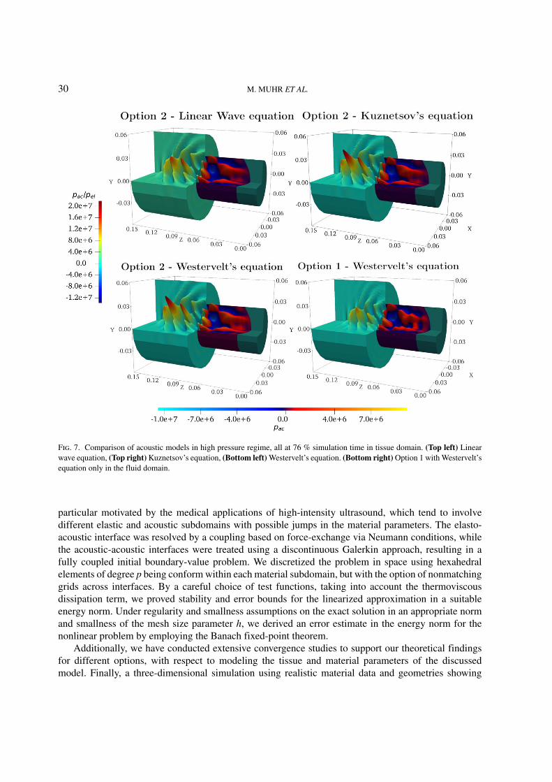
30 M. MUHR ET AL.

Fig. 7. Comparison of acoustic models in high pressure regime, all at 76 % simulation time in tissue domain. (Top left) Linearwave equation, (Top right) Kuznetsov’s equation, (Bottom left) Westervelt’s equation. (Bottom right) Option 1 with Westervelt’sequation only in the fluid domain.

particular motivated by the medical applications of high-intensity ultrasound, which tend to involvedifferent elastic and acoustic subdomains with possible jumps in the material parameters. The elasto-acoustic interface was resolved by a coupling based on force-exchange via Neumann conditions, whilethe acoustic-acoustic interfaces were treated using a discontinuous Galerkin approach, resulting in afully coupled initial boundary-value problem. We discretized the problem in space using hexahedralelements of degree p being conform within each material subdomain, but with the option of nonmatchinggrids across interfaces. By a careful choice of test functions, taking into account the thermoviscousdissipation term, we proved stability and error bounds for the linearized approximation in a suitableenergy norm. Under regularity and smallness assumptions on the exact solution in an appropriate normand smallness of the mesh size parameter h, we derived an error estimate in the energy norm for thenonlinear problem by employing the Banach fixed-point theorem.

Additionally, we have conducted extensive convergence studies to support our theoretical findingsfor different options, with respect to modeling the tissue and material parameters of the discussedmodel. Finally, a three-dimensional simulation using realistic material data and geometries showing

A DISCONTINUOUS GALERKIN COUPLING FOR NONLINEAR ELASTO-ACOUSTICS 31

Fig. 8. Model comparison of pressure signal at (Left) axis of symmetry of tissue domain at 76 % of simulation time. (Right)Same comparison, but over time at fixed point p = (0, 0, 0.12) m.

the propagation of ultrasound waves into human tissue closes the loop to the original motivation of thework.

Future research on the topic will be concerned with the analysis and simulation of problemsincluding nonlinear effects, not only in the acoustic, but also elastic regime, and the simulation ofultrasound heating by an additional coupling with a temperature model.

Acknowledgements

We would like to thank the reviewers for their careful reading of our manuscript and for the insightfulremarks. M. Muhr and B. Wohlmuth acknowledge the financial support provided by the DeutscheForschungsgemeinschaft under the grant number WO 671/11-1.

References

Antonietti, P. F., Bonaldi, F. & Mazzieri, I. (2020a) A high-order discontinuous Galerkin approach to theelasto-acoustic problem. Comput. Methods Appl. Mech. Eng., 358, 112634.

Antonietti, P. F., Mazzieri, I., Muhr, M., Nikolic, V. & Wohlmuth, B. (2020b) A high-order discontinuousGalerkin method for nonlinear sound waves. J. Comput. Phys., 415, 109484.

Antonietti, P. F., Ferroni, A., Mazzieri, I., Paolucci, R., Quarteroni, A., Smerzini, C. & Stupazzini, M.(2018) Numerical modeling of seismic waves by discontinuous spectral element methods. ESAIM Proc. Surv.,61, 1–37.

Antonietti, P. F., Mazzieri, I., Quarteroni, A. & Rapetti, F. (2012) Non-conforming high order approxima-tions of the elastodynamics equation. Comput. Methods Appl. Mech. Eng., 209, 212–238.

Brenner, S. & Scott, R. (2008) The Mathematical Theory of Finite Element Methods, vol. 15. New York: SpringerScience & Business Media.

32 M. MUHR ET AL.

Brivadis, E., Buffa, A., Wohlmuth, B. & Wunderlich, L. (2015) Isogeometric mortar methods. Comput.Methods Appl. Mech. Eng., 284, 292–319.

Brunnhuber, R., Kaltenbacher, B. & Radu, P. (2014) Relaxation of regularity for the Westervelt equation bynonlinear damping with application in acoustic–acoustic and elastic–acoustic coupling. Evol. Equ. ControlTheory, 3, 595–626.

Cangiani, A., Georgoulis, E. H. & Houston, P. (2014) hp-version discontinuous Galerkin methods on polygonaland polyhedral meshes. Math. Models Methods Appl. Sci., 24, 2009–2041.

Chung, J. & Hulbert, G. (1993) A time integration algorithm for structural dynamics with improved numericaldissipation: the Generalized-α method. J. Appl. Mech., 60, 371–375.

Di Pietro, D. A. & Ern, A. (2012) Mathematical Aspects of Discontinuous Galerkin Methods, vol. 69. Berlin,Heidelberg: Springer.

Engquist, B. & Majda, A. (1977) Absorbing boundary conditions for numerical simulation of waves. Proc. Natl.Acad. Sci., 74, 1765–1766.

Epshteyn, Y. & Rivière, B. (2007) Estimation of penalty parameters for symmetric interior penalty Galerkinmethods. J. Comput. Appl. Math., 206, 843–872.

Erlicher, S., Bonaventura, L. & Bursi, O. S. (2002) The analysis of the generalized-α method for non-lineardynamic problems. Comput. Mech., 28, 83–104.

Felippa, C. A., Park, K. & Ross, M. (2011) A classification of interface treatments for FSI. Fluid StructureInteraction II. Berlin, Heidelber: Springer, pp. 27–51.

Flemisch, B., Kaltenbacher, M. & Wohlmuth, B. I. (2006) Elasto–acoustic and acoustic–acoustic coupling onnon-matching grids. Int. J. Numer. Methods Eng., 67, 1791–1810.

Hamilton, M. F. & Blackstock, D. T. (1998) Nonlinear Acoustics, volume 1. San Diego: Academic Press.Hou, G., Wang, J. & Layton, A. (2012) Numerical methods for fluid–structure interaction—a review. Commun.

Comput. Phys., 12, 337–377.Kaltenbacher, B. & Lasiecka, I. (2009) Global existence and exponential decay rates for the Westervelt equation.

Discrete Contin. Dyn. Syst. Ser. S, 2, 503.Kaltenbacher, B. & Peichl, G. (2016) The shape derivative for an optimization problem in lithotripsy. Evol.

Equ. Control Theory, 5, 399.Kaltenbacher, M. (2007) Numerical Simulation of Mechatronic Sensors and Actuators, vol. 2. Berlin, Heidel-

berg: Springer.Kennedy, J. E. (2005) High-intensity focused ultrasound in the treatment of solid tumours. Nat. Rev. Cancer, 5,

321–327.Kuznetsov, V. P. (1970) Equations of nonlinear acoustics. Sov. Phys. Acoustics, 16, 467–470.Lee, D., Koizumi, N., Ota, K., Yoshizawa, S., Ito, A., Kaneko, Y., Matsumoto, Y. & Mitsuishi, M.

(2007) Ultrasound-based visual servoing system for lithotripsy. 2007 IEEE/RSJ International Conference onIntelligent Robots and Systems. San Diego, CA: IEEE, pp. 877–882.

Li, Z. C. (1998) Lagrange Multipliers and Other Coupling Techniques. Boston, MA: Springer US,pp. 209–224.

Maier, B. (2020) Error analysis for space and time discretizations of quasilinear wave-type equations. Ph.D. Thesis,Karlsruhe Institute of Technology, Germany.

Mazzieri, I., Stupazzini, M., Guidotti, R. & Smerzini, C. (2013) SPEED: SPectral elements in elastodynamicswith discontinuous Galerkin: a non-conforming approach for 3D multi-scale problems. Int. J. Numer. MethodsFluids, 95, 991–1010.

Meyer, S. & Wilke, M. (2011) Optimal regularity and long-time behavior of solutions for the Westervelt equation.Appl. Math. Optim., 64, 257–271.

Mizohata, K. & Ukai, S. (1993) The global existence of small amplitude solutions to the nonlinear acoustic waveequation. J. Math. Kyoto Univ., 33, 505–522.

Muhr, M., Nikolic, V. & Wohlmuth, B. (2021). A discontinuous Galerkin coupling for nonlinear elasto-acoustics. arXiv preprint arXiv:2102.04311v2. Extended arXiv version.

A DISCONTINUOUS GALERKIN COUPLING FOR NONLINEAR ELASTO-ACOUSTICS 33

Muhr, M., Nikolic, V., Wohlmuth, B. & Wunderlich, L. (2019) Isogeometric shape optimization for nonlinearultrasound focusing. Evol. Equ. Control Theory, 8, 163–202.

Nikolic, V. & Wohlmuth, B. (2019) A priori error estimates for the finite element approximation of Westervelt’squasi-linear acoustic wave equation. SIAM J. Numer. Anal., 57, 1897–1918.

Ortner, C. & Süli, E. (2007) Discontinuous Galerkin finite element approximation of nonlinear second-orderelliptic and hyperbolic systems. SIAM J. Numer. Anal., 45, 1370–1397.

Schötzau, D., Schwab, C. & Toselli, A. (2002) Mixed hp-dgfem for incompressible flows. SIAM J. Numer.Anal., 40, 2171–2194.

Shevchenko, I., Kaltenbacher, M. & Wohlmuth, B. (2012) A multi-time stepping integration method for theultrasound heating problem. ZAMM J. Appl. Math. Mech./Zeit. Angew. Math. Mech., 92, 869–881.

Skolarikos, A., Alivizatos, G. & de la Rosette, J. (2006) Extracorporeal shock wave lithotripsy 25 years later:complications and their prevention. Eur. Urol., 50, 981–990.

Stacey, R. (1988) Improved transparent boundary formulations for the elastic-wave equation. Bull. Seismol. Soc.Amer., 78, 2089–2097.

Stupazzini, M., Paolucci, R. & Igel, H. (2009) Near-fault earthquake ground-motion simulation in the Grenoblevalley by a high-performance spectral element code. Bull. Seismol. Soc. Amer., 99, 286–301.

Westervelt, P. J. (1963) Parametric acoustic array. J. Acoust. Soc. Amer., 35, 535–537.Wick, T. & Wollner, W. (2020) Optimization with nonstationary, nonlinear monolithic fluid–structure interaction.

Int. J. Numer. Methods Eng., 122, 5430–5449.

B. Further ArticlesB.1. Elasto-acoustic modelling and simulation for the seismic

response of structures: The case of the Tahtalı dam in the2020 Izmir earthquake

136

Elasto-acoustic modelling and simulation for theseismic response of structures: The case of the

Tahtalı dam in the 2020 Izmir earthquakeIlario Mazzieri, Markus Muhr, Marco Stupazzini and Barbara Wohlmuth

Seismic hazard analysis, especially in regions of high ground motion activity, is crucialfor risk assessment and seismic design of building structures. This article deals with theconstruction and application of a numerical, elasto-acoustic model to simulate the effectsa seismic event has on dam structures. As a concrete case study the response of theTahtalı dam, located in Turkey near the city of İzmir, during the magnitude Mw = 7earthquake from the 30th of October 2020 is analyzed [59]. Real topography and grounddata [155, 290] is used to create a realistic model, which is then validated against actualseismograph-measurements [1] from the event. Due to the generality of the model, theachieved simulation capabilities lay the foundations for further simulation based seismicanalyses.For this article we utilize the elasto-acoustic- and DG-coupling capabilities of SPEED

in order to simulate the dam, the underlying layers of ground, each with possibly differentmaterial parameters, as well as the reservoir lake behind the dam. The elasto-acousticmodel and discretization hereby are adopted from [7, II], where in this article the focuslies on the application and the incorporation of real data. First of all, the topography ofthe surrounding area of the dam is resolved from satellite altitude data [155]. A CAD-model of the dam is then placed in the topography and a complex mesh is generatedto capture the necessary features of the solid/elastic geometry. The elasto-acousticinterface is used to incorporate the influence of the water in the reservoir-lake, being theacoustic medium. To model the seismic source, inversion-data about the actual seismicfault plane are used for a stress-glut source model. The final source-to-site model spansseveral length scales, which are resolved by means of local mesh refinement and theDG approach to couple non-matching sub-meshes. The resulting all-in-one simulationis compared also to a more classical approach using a deconvolved seismograph signalas a plane wave input. Outputs of the simulations feature peak ground maps of e.g.displacement and velocity and deformations of the dam, relevant from a seismologicaland engineering point of view to judge the safety of the dam.After the introduction, Sec. 2 introduces the elasto-acoustic mathematical model and

Sec. 3 the numerical methods used for spatial and temporal discretization. In Sec. 4, adescription of the seismic event, the region of interest and the dam itself is given, placingit into a broader context. Sec. 5 then contains a description of the real-data basedgeometry acquisition and the meshing. In Sec. 6, the different numerical experimentsare then conducted, evaluated and compared. Sec. 7 finally gives a conclusion and anoutlook to further work to be done in this direction ultimately aiming for the goal of aseismic hazard analysis of the whole region.I was significantly involved in finding the ideas and carrying out the scientific work

presented in this article including the write-up, except for Sec. 4. Furthermore I was incharge of the numerical part of the article, i.e. acquisition, treatment and evaluation ofdata, implementation and conduction of the simulations and the creation of the figures.

137

Permission to include:

Mazzieri, Ilario, Markus Muhr, Marco Stupazzini, and Barbara WohlmuthElasto-acoustic modelling and simulation for the seismic response of struc-tures: The case of the Tahtalı dam in the 2020 Izmir earthquakesubmitted to: Journal of Computational Physics

Included is the arXiv preprint version.

138

The above page is a copy from the webpagehttps://arxiv.org/help/policies/submission_agreement

Date: 22.11.2021

ELASTO-ACOUSTIC MODELLING AND SIMULATION FOR THE

SEISMIC RESPONSE OF STRUCTURES: THE CASE OF THE

TAHTALI DAM IN THE 2020 IZMIR EARTHQUAKE

ILARIO MAZZIERI1, MARKUS MUHR∗,2, MARCO STUPAZZINI3, AND BARBARA WOHLMUTH2

1MOX, Dipartimento di Matematica, Politecnico di Milano, Milano, Italy2Department of Mathematics, Technical University of Munich, Garching, Germany

3Munich RE, Munchener Ruckversicherungs-Gesellschaft, Munich, Germany

Abstract. As a mean to assess the risk dam structures are exposed to during earth-quakes, we employ an abstract mathematical, three dimensional, elasto-acoustic coupledwave-propagation model taking into account (i) the dam structure itself, embedded into(ii) its surrounding topography, (iii) different material soil layers, (iv) the seismic sourceas well as (v) the reservoir lake filled with water treated as an acoustic medium. As a casestudy for extensive numerical simulations we consider the magnitude 7 seismic event of the30th of October 2020 taking place in the Icarian Sea (Greece) and the Tahtalı dam around30 km from there (Turkey). A challenging task is to resolve the multiple length scales thatare present due to the huge differences in size between the dam building structure andthe area of interest, considered for the propagation of the earthquake. Interfaces betweenstructures and highly non-conforming meshes on different scales are resolved by means ofa discontinuous Galerkin approach. The seismic source is modeled using inversion dataabout the real fault plane. Ultimately, we perform a real data driven, multi-scale, fullsource-to-site, physics based simulation based on the discontinuous Galerkin spectral el-ement method, which allows to precisely validate the ground motion experienced alongthe Tahtalı dam, comparing the synthetic seismograms against actually observed ones. Acomparison with a more classical computational method, using a plane wave with datafrom a deconvolved seismogram reading as an input, is discussed.

1. Introduction

With the continuous growth of computational power in the last decades, physics basedsimulation (PBS) emerged as an aspiring, alternative approach to ground motion predic-tion equations (GMPEs), which has already been applied to seismic scenarios at varioussites including the United States [80, 81], Japan [37, 45], New-Zealand [26, 52], Turkey[44], China [4], the Netherlands [64], Italy [32]. PBS aims at describing, as reliably aspossible, the seismic wave propagation problem and therefore it is crucial, on the one hand,to properly characterize the mechanical properties of the different portion of the compu-tational domain and, on the other, to have a reliable seismic excitation source, see, e.g.[18, 38, 44, 64, 68, 87]. Because of the intrinsically high epistemic uncertainties involved inthe construction of 3D numerical models, those need to be verified and validated againstavailable earthquake recordings, cf. e.g. [12, 19, 65]. Nowadays, thanks to the availabilityof openly accessible data, as for example [30, 83], this challenge can be tackled in spe-cific regions of the world. PBS generates synthetic time histories of displacement, velocity,acceleration and also other engineering relevant quantities, such as strains, stresses androtations. The numerical methods used are most often finite differences [24, 56, 69], finiteelements [11], finite volumes [17, 28, 29, 67] or, as used here in combination with a linear

Key words and phrases. Earthquake simulation, elasto-acoustic coupling, DG-method, water-dam-structure.∗Corresponding author: Markus Muhr, muhr@ma.tum.de.

1

arX

iv:2

110.

1587

5v1

[m

ath.

NA

] 2

9 O

ct 2

021

2 I. MAZZIERI, M. MUHR, M. STUPAZZINI AND B. WOHLMUTH

visco-elastic model, spectral elements in conforming [38, 49, 77] but also discontinuous ways[7, 25, 34].

In this work, we simulate within a single computational model a full seismic event, fromsource-to-site, and study the effects of ground shaking on a larger building structure. Wetherefore employ a, mathematically general seismic wave-popagation model to a compu-tational domain consisting of several layers of soil, each with its own material propertiesand with lengths up to the 100 km scale. On the small scale of 10-100 m, with the samemathematical model, we consider a, comparably small, dam structure in order to analyzeits performance under the seismic impact of an earthquake. Together this results in alarge, multi-scale problem. The challenge of coupling the multiple, non-conforming meshesof different sizes [57] is tackled by means of the discontinuous Galerkin spectral elementmethod [8]. In addition, two more important factors are considered for properly simulatinga dam subjected to seismic excitation: (i) the structure is embedded into its surround-ing and therefore the topography should be accurately described, resulting in complexgeometries and hence mesh structures, (ii) in contrast to free-standing typical edifices [48]where the surrounding air is most often ignored, the seismic behaviour of the reservoir lakelocated behind the dam cannot be neglected, and therefore a coupled elasto-acoustic wave-propagation problem needs to be solved. These two factors are considered in this work bymaking use of digital elevation maps, that can be obtained freely from [46, 70], to obtaina realistic topographic profile and second by resolving the reservoir lake behind the damas well. As a matter of fact, within the reservoir lake the propagation of acoustic waveswill be modeled by a scalar wave equation. The elasto-acoustic dam-water- and ground-water-interfaces are equipped with force exchange coupling conditions. For a mathematicaldiscussion of the coupled problem, we refer to [5, 35], while [60] considers the problemeven in a nonlinear, acoustic context. As a seismic source we consider a kinematic rupturemodel with a prescribed slip-vector and moment-tensor distribution across a fault plane[33]. The model is also compared to another sourcing mechanism using a plane wave inputof a recorded seismogram.

The mathematical model and the numerical simulation are validated with respect to thespecific magnitude 7 seismic event that took place on the 30th of October in 2020 at around11:51 h. Its hypocenter lies at 37.8973N, 26.7953 E in the Icarian Sea northern the isle ofSamos, Greece. Approximately 30 km north-east of it on Turkish mainland there lies theTahtalı-dam with its fresh-water reservoir. Due to its proximity to the source, the dam wasseverely threatened by the seismic event; however, the reconnaissance team provided theevidence that no severe damages occurred [23]. Besides the topography data mentionedabove, in this work, we make use of the large amount of available data regarding the seismicfault source [83] for a realistic simulation of the earthquake’s origin, recorded seismogramsmade freely available by the Turkish Disaster & Emergency Management Authority AFAD[1] and ground material data [83], in order to validate our model and to yield a realisticdescription of and reliable results for the considered case study.

Our simulations have been obtained using the code SPEED [8, 55, 77] employing hexa-hedral meshes with higher order spectral elements. Sub-meshes with non-matching grids,e.g., at material interfaces with different refinements are coupled using a discontinuousGalerkin approach. Real case simulations as in the present case can easily result in millionsof degrees of freedom in space and time, especially when considering higher polynomial or-ders. Therefore SPEED employs a hybrid MPI/OpenMP parallel implementation allowingto harness a large amount of computational resources.

SIMULATION OF SEISMIC RESPONSE OF DAMS 3

We organize the rest of the paper as follows. Section 2 introduces the elasto-acousticmathematical model, the equations, boundary- and coupling conditions used. In Section 3,we discuss the adopted discretization in space and time. We derive the semi-discrete form ofthe model equations by means of spectral elements and introduce a standard time integra-tion scheme. In Section 4, we briefly describe the seismic event adopted as a case study inthis work. Section 5, is then devoted to the geometry acquisition (topography/mechanicalproperties) from real data, and some comments on the mesh generation are given. Finally,the numerical simulations and results are discussed in Section 6, where different simulationmethods are presented, validated and finally compared.

2. Mathematical model

We begin by defining the mathematical models used to describe the seismic problem, be-ing the elastic model for the solid parts (soil layers and dam in the specific case study) andacoustic model equations for the fluid part (reservoir lake) each with their correspondingsets of boundary, initial and interface conditions. The computational domain together withits individual material subdomains is then also introduced where, without loss of generality,we refer to the specific case study of the Tahtalı-dam considered in this work. For the wholemanuscript, we will denote scalar quantities by regular, greek or latin characters, vectorialquantities will be bold and underlined and tensorial quantities will just be bold.

Mathematical model. As a mathematical model for the description of the individualsolid parts/subdomains Ωe,i, i = 1, 2, . . . , Ne of the problem, we use the equations ofdisplacement-based linear elasticity (2.1) subdomain-wise with Hook’s law σ = λtr(ε)1 +2µε as constitutive relation [48, 53], ε = 1

2

(∇u +∇u>

)being the symmetric gradient of

the displacement u, and λ and µ being subdomain-wise constant Lame-parameters, reading

λ = λ(x) = λi, for x ∈ Ωe,i and i = 1, 2, . . . , Ne,

µ = µ(x) = µi, for x ∈ Ωe,i and i = 1, 2, . . . , Ne.

Parts of ∂Ωe on the top surface with no overlying body of water (green and white visiblesurfaces in Fig. 1, right), summarized as Γe,N are treated as free surfaces (2.2), the fourartificial boundaries in x and y directions as well as the plane bottom surface in z-direction(brown in Fig. 1) are equipped with absorbing boundary conditions (2.3). Herein t∗ is afictitious traction force reducing the amount of artificial reflections originating from thesesurfaces [8, 33, 76]. Parts of ∂Ωe that are interfaces to the acoustic domain Ωa, denotedby ΓEA (orange in Fig. 1), are equipped with non-homogeneous Neumann conditions (2.4)acting as force-exchange interface conditions to the acoustic field [5, 60]. Here the shorthand notation of

ψ := ψ +b

c2ψ

is introduced. On internal interfaces between the individual elastic sub-domains Ωe,i, col-lectively denoted by ΓDG (not visible in Fig. 1, however analogously to elasto-acoustic-interfaces but between ground and dam subdomain), transmission conditions (2.5) areemployed, where

[[σ]] := (σ+ − σ−)n, [[u]] := (u+ − u−)⊗ n.

Hereby n is the interface normal with arbitrary but fixed orientation and ι±(x) := limt↓0 ι(x±tn), ι ∈ σ,u. Finally suitable initial conditions (2.6) for displacement and velocity v = uare prescribed, completing the elastic problem.

4 I. MAZZIERI, M. MUHR, M. STUPAZZINI AND B. WOHLMUTH

ρe,i

(u + 2ζiu + ζ2

i u)−∇ · σ(u) = f , in Ωe,i × (0, T ],(2.1)

σn = 0, on Γe,N × (0, T ],(2.2)

σn = t∗, on Γe,ABC × (0, T ],(2.3)

σn = −ρa˙ψn, on ΓEA × (0, T ],(2.4)

[[σ]] = 0, [[u]] = 0, on ΓDG × (0, T ],(2.5)

(u, u) = (u0,u1), at Ωe × 0.(2.6)

In the above system of equations ρe,i are the mass densities of the subdomains Ωe,i, i =1, 2, . . . , Ne, ρa is the mass density for the acoustics domain and ζi, i = 1, . . . , Ne are vis-cous damping factors proportional to the inverse of time. For future use, we also introducethe compressional vp and shear vswave velocities defined as vp,i =

√(λi + 2µi)/ρe,i and

vs,i =√µi/ρe,i for i = 1, . . . , Ne, respectively.

In the acoustic subdomain Ωa, the linear, damped wave equation (2.7) in potentialform, ψ being the acoustic potential, is used to model the propagation of pressure waveswith speed of sound c and damping coefficient b. On free water-surfaces (Fig. 1 left, blue)homogeneous Neumann conditions (2.8), on artificially generated surfaces, resulting fromthe cut-out of Ω from the Earth (Fig. 1 backside, where the lake is cut-off), absorbingboundary conditions (2.9) [31, 75] and on interfaces with the elastic bodies Ωe,i (Fig. 1right, orange) interface conditions (2.10) once more as in [5, 60] are imposed. Again,suitable initial conditions (2.11) complete the acoustic problem.

1

c2ψ −∆ψ = 0, in Ωa,i × (0, T ],(2.7)

∇ψ · n = 0, on Γa,N × (0, T ],(2.8)

∇ψ · n = −1

cψ, on Γa,ABC × (0, T ],(2.9)

∇ψ · n = −u · n, on ΓEA × (0, T ],(2.10)

(ψ, ψ) = (ψ0, ψ1), at Ωa × 0(2.11)

Note that for all material parameters ι ∈ ρe,i, ρa, ζi, λi, µi, c, b defined above, we assumethe existence of uniformly positive and finite bounds above and below. Note that quantitiesof interest like acoustic or seismic/elastic pressure can be computed from the solutions of

the above models via pac = ρaψ, pel = −13

∑3i=1 σii in a post processing step.

Remark 1. We remark that ΓDG does not have to contain all internal elastic interfacesnecessarily and hence the (discontinuous Galerkin) transmission conditions do not haveto be applied to all of them. As an alternative, if grids are matching, also a conformingcoupling would be possible.

Computational domain. For the computational core-domain Ω in the specific case studywe choose an, in x − y direction rectangular, cut-out of the Earth around the location ofthe dam. In z-direction Ω is limited by a plane surface at a given depth below the Earthsurface at bottom, while on top the topographic profile of the Earth is used. In a secondstep, Ω is divided into an acoustic part Ωa consisting of a portion of the dam reservoir lakelying within Ω, and the remaining part Ωe consisting of solid ground (mountain range, soillayers) and the dam itself. The elastic subdomain Ωe is then further divided into individ-ual subdomains Ωe,i, i = 1, 2, . . . , Ne, each representing an individual material block, withits own set of constant material parameters, which are possibly discontinuous across theinterfaces between the blocks. As a prime example, the dam structure would be one suchsubdomain while the surrounding ground would be an other. See Fig. 1, left, for a graphical

SIMULATION OF SEISMIC RESPONSE OF DAMS 5

depiction of the domain of interest with Ne = 2 elastic subdomains.

Figure 1. (left) Computational domain with three subdomains. Green: Solid groundΩe,1, White: Solid dam structure Ωe,2, Blue: Acoustic water domain Ωa. (right)Highlighting boundary/interface conditions: Brown: Absorbing boundary conditions (all4 sides, incl. the water cut-off surface plus bottom surface), Orange: Elasto-Acousticcoupling interface., Green, White, Water top surface: Free surfaces, Non visible:Interfaces between Ωe,1 and Ωe,2; they are analogous to the elasto-acoustic interfaces.

3. Numerical methods

This section starts with a description of the spatially discrete setting used to approximatea weak solution to the seismic problem (2.1)-(2.11). We then derive the semi-discreteequation in variational and matrix-vector form and end with some notes about the usedtime integration scheme.

3.1. Spatial discretization

In this subsection, the mesh(es) to be used and the finite element spaces built on themare introduced. We hereby closely follow [60], where more details on mesh assumptionsbeing sufficient to prove convergence in a similar setting are given.

Meshing. The meshing of the computational domain Ω is done sub-domain wise. Thismeans that each Ωe,i as well as Ωa is subdivided into a mesh Te,i, resp. Ta of hexahe-dral elements individually. While we assume that also after meshing the discrete interfacemanifolds do coincide - seen from both sides of the interfaces - the individual meshes onthose manifolds do not have to. Hence, on the interface the mesh from one side could be arefinement of the mesh from the other side or, for example at a flat interface, could also bea staggered or even completely different mesh. Such non-conformities will be treated by adiscontinuous Galerkin approach for the interface coupling.

Discrete spaces. Our goal is to approximate a weak solution to the seismic problem bymeans of spectral finite elements. Within each subdomain Ωe,i and Ωa, this is done in aconforming way, while only at (part of) the interfaces the aforementioned DG approach willbe used. This goes hand in hand with the different material properties of the individualsub-domains, and it also allows to keep the amount of degrees of freedom low within thesub-domains, while being flexible at the interfaces.

We denote by Ve,ih the space of discrete ansatz-functions on the i-th elastic subdomain,

i = 1, 2, . . . , Ne, which are elementwise polynomials of order pi when transformed back tothe reference element. By Ve

h we denote the space of global elastic ansatz-functions, which,restricted to any of the subdomains, are within the subdomain’s ansatz-space. Similar V a

h

6 I. MAZZIERI, M. MUHR, M. STUPAZZINI AND B. WOHLMUTH

denotes the ansatz-space for the acoustic subdomain. The setting hence directly corre-sponds to the one in [60] where the overall coupled elasto-acoustic problem, even though ina medical ultrasound setting, including additional non-linear acoustic terms, was analyzedregarding stability and convergence w.r.t. spatial refinement. Therein also further mathe-matical details are given in a similar setting.

Semi-discrete form. With introducing the mean operator defined as:

σ =1

2(σ+ + σ−), u =

1

2(u+ + u−).

in addition to the already defined jump operator, the semi-discrete variational problem isgiven by:

For any time t ∈ (0, T ] find (uh, ψh) ∈ Veh × V a

h such that for all (wh, φh) ∈ Veh × V a

hthere holds:

Ne∑

i=1

[(ρe,iuh,wh)Ωe,i + (ρe,i2ζiuh,wh)Ωe,i + (ρe,iζ

2i uh,wh)Ωe,i + (σ(uh), ε(wh))Ωe,i

]

−(t∗h,wh)Γe,ABC− 〈σ(uh), [[vh]]〉ΓDG

− 〈[[uh]] , σ(vh)〉ΓDG+ 〈χ [[uh]] , [[vh]]〉ΓDG

(3.1)

+(ρa

˙ψhn,wh

)ΓEA

+ (uh · n, φh)ΓEA

+(c−2ψh, φh

)Ωa

+ (∇ψh,∇φh)Ωa +(c−1ψh, φh

)Γa,ABC

= (fh,wh)Ωe

and uh(0) = u0 = 0, uh(0) = u1 = 0, ψh(0) = ψ0 = 0 and ψh(0) = ψ1 = 0, which corre-sponds to an initial state at rest for the solid as well as for the acoustic quantities.

Finally, for any face in ΓDG, defined as the intersection between opposite elemental faces,we define the penalty parameter χ as:

χ|F := λ+ 2µAp2F

hF

being F a DG face shared by the mesh elements E+ and E−, pF = maxp+, p−, hF =minh+, h−, qA the harmonic average of the quantity q, and β a positive real numberat our disposal, cf. [8, 25, 60].

Matrix-Vector form. After representing the discrete trial functions uh and ψh as well astheir temporal derivatives in the nodal finite element basis, denoting the coefficient vectorsby (abuse of notation) also uh and ψ

h, the following system of ODEs in matrix-vector form

is directly obtained from (3.1):(M(2)

e 0

0 M(2)a

)(uh

ψh

)=−

(M(1)

e 00 0

)(uh

ψh

)−(M(0)

e 00 0

)(uh

ψh

)

+

(−Ke + D + D> −P 0

0 −Ka

)(uh

ψh

)(3.2)

−(

0 EA 0

)(uh˙ψh

)−(

0 00 Ca + Ca,ABC

)(uh

ψh

)+

(T∗h0

)+

(Fh

0

)

with initial conditions:

(uψ

)=

(u

ψ

)=

(00

)

Herein M(1)e and M

(0)e are subdomain-wise scaled versions of the standard mass-matrix

M(2)e for the elastic part of the problem. Due to the DG approach for the interface coupling,

SIMULATION OF SEISMIC RESPONSE OF DAMS 7

they are block-diagonal with one block per subdomain. In fact, due to the use of spectralelements, they even become diagonal. This property is not only advantageous to be ex-ploited by the time stepping scheme but also allows to denote the aforementioned scalingusing the diagonal matrix Z, which has entries ζi for each degree of freedom belonging to

the elastic subdomain Ωe,i. With that, the scaled mass matrices read M(1)e = 2ZM

(2)e and

M(0)e = Z2M

(2)e . Analogously M

(2)a is the standard mass-matrix for the acoustic part. Ka

resp. Ke denote stiffness-matrices for the scalar resp. vectorial case, Ca incorporates theb-damping of the acoustic equation. On the right hand side D and P are the matrices stem-ming from the inter-elastic DG coupling, where P contains the penalization term, whileE and A contain the coupling terms between the elastic and acoustic domains. FinallyCa,ABC is a boundary mass-matrix used in the implementation of the acoustic absorbingboundary conditions, T∗h incorporates the elastic absorbing boundary conditions and Fh

the elastic source term inducing the earthquake (cf. Sec. 6 for different source models).

3.2. Time integration

The basis scheme used for time integration is the Leap-Frog scheme in its full-steppredictor-corrector form [42]. After the prediction step

φ(n+1) = φpred

= φ(n) + ∆tφ(n)

+1

2∆t2φ

(n), φ

pred= φ

(n)+

1

2∆tφ

(n)

for φ ∈ uh, ψh the right hand side of (3.2) can be evaluated using the predicted values

(and the previous timestep value for ψh

within˙ψh). One then conducts a solver step for

the left hand side variables u(n+1)h and ψ

(n+1)

hfollowed by the correction step

φ(n+1)

= φpred

+1

2∆tφ

(n+1)

again φ ∈ uh, ψh.

To take into account the multiscale nature in time, we also employ a simple local time-stepping approach for the acoustic part of the problem similar to [74]. Especially in thevicinity of the inclined dam surface that is under water (cf. Fig. 4, right) water elementsbecome quite thin hence requiring small timesteps that are not necessary in the remainingregion of the problem, especially the huge land masses Ωe,i of seismic propagation. Hence,within each regular time step of size ∆t the solution of the acoustic equation within Ωa

consisting of prediction, evaluation, solving and correction is internally repeated within aloop of nloc timesteps of size ∆t

nlocbefore the next regular step for the elastic portion of the

problem is conducted. In the presented simulation cases a value of nloc = 10 yields goodresults.

4. Seismic scenario description

We now provide some selected information about the specific, real seismic event thatwill serve as a case study for the mathematical model and numerical methods described inSec. 2 and 3. The event was chosen due to the large amount of seismograms recorded andtherefore allowing a proper validation of the simulation.

The Samos Island (Aegean Sea) earthquake struck at 14:51 local time in Turkey, on 30October 2020. Severe damages have been observed in some densely populated districts ofIzmir (Bayraklı, Bornova, Karsıyaka and Konak), and 118 fatalities have been reported.The present event occurred in the cross-border region between the eastern Aegean Seaislands and Western Turkey, which is among the most seismically active areas in EasternMediterranean and has been the site of devastating earthquakes in both recent and historical

8 I. MAZZIERI, M. MUHR, M. STUPAZZINI AND B. WOHLMUTH

times, see [40]. The fault that ruptured during the mainshock is located offshore thenorthern coast of Samos Island, and it was previously identified as Kaystrios Fault (seeGreDaSS database [20] and the GEM-Faults database [78]). The geometric characteristicsof the Kaystrios Fault are: strike in the range 260° to 290°, dip 45° to 70° and rake in therange -100° to -80°, while the maximum depth of the fault is estimated as 14.5 km.

The mainshock was well recorded by the broadband seismic networks of Greece andTurkey, and 35 records are located within 100 km distance from the epicenter [22, 23, 27,63, 88]. Between October 31st and November 6th a group of engineers assembled by the

Izmir Regional Directorate of State Hydraulic Works (DSI) and a reconnaissance team fromMETU visited dam sites to document the performance of earth-fill and rock-fill dams shakenby the event. After a detailed inspection of six small to medium size earth-fill and rock-fill dams including the Tahtalı dam, no apparent damage was reported by reconnaissanceteams.

As reported by [82], the Tahtalı dam is a rockfill dam on the Tahtalı River near Gumuldur

County in the Izmir Metropolitan Area. It has a 54.4 m height from river bed. When thereservoir is at maximum capacity, the facility impounds 306.6 hm3 of water in its reservoir.Its construction was finished in 1999. It was designed to provide domestic water with anactive volume of 287 hm3. As reported by [82], the Tahtalı dam is only 1.9 km away from anactive fault and, according to the seismic hazard analyses performed, it will be subjectedto a peak ground acceleration of 0.277 g by an earthquake of Mw 5.7. The Tahtalı dam isat second place, after Gordes dam, when regarding the total capacity of the reservoir andone of the most critical dams in the Izmir Metropolitan Area.

5. Geometry acquisition and mesh generation

The methods described in this section are general and can easily be adopted to differentscenarios. However, the individual steps are motivated and illustrated based on the casestudy discussed in Sec. 4.

Digital elevation map data. In the presently examined case study, the topography of thesurrounding area of the Tahtalı-dam is obtained from the SRTM Digital Elevation Databaseof CGIARCSI [46], which contains topographic elevation data in a 3 arc second grid.On the left-hand side of Fig. 2 a contour plot of a roughly 3 km×2 km area around theTahtalı-dam is shown, while on the right-hand side of Fig. 2, the respective area in a satelliteview for a clear image of the dam location is given.

Map data: Google, Imagery ©2021CNES/Airbus, Maxar Technologies, Mapdata ©2021

Figure 2. (left) Topographic map of the region around the Tahtalı-dam with referencecoordinate-system. Data source [46]. (right) Satellite view of the same area. The redmarker is located at 38.0888 N, 27.0415 E. Image source [39].

SIMULATION OF SEISMIC RESPONSE OF DAMS 9

CAD model construction. Starting from the elevation point-cloud data, a volumetricobject is constructed and afterwards modified in order to add the dam and the water,and finally proceeding with the meshing. To tackle this challenge the software Cubit[13, 21], which also features some CAD-capabilities, was used firstly for the surface- andthen volume-reconstruction.Using the point cloud elevation data, a spline-surface approximating the topography iscreated, see Fig. 3. For the bottom surface a rectangle in the x-y-plane directly belowthe topographic spline-surface at depth z = −300 m is used. The four sides remaining toclose the volume are flat surfaces and connect the four boundary curves of bottom and topsurfaces.

Figure 3. (left) Orange: Elevation point data obtained from [46], Blue: x − y-spline curves, Green: Spline net-surface approximation of topography. (right) Volumetricground object with closing sides (and bottom surface at z = −300 m) in brown.

Once the topography is available, the dam is added, see Fig. 4, left. The dam is placedin the proper location within the topography and, by means of simple boolean intersec-tion/subtraction as well as downward extrusion operations between the two volumes, is“naturally” finally embedded into the surrounding area. Fig. 4, middle, shows the portionof the dam after the operations within the topography.

Figure 4. (left) CAD-model of a gravitational dam. The blue lines (compare to figureright) are the intersection curves between the dam and ground model. (middle) Dam-structure embedded into surface topography. (right) Cross section View on CAD-modelof ground, dam and water. Due to the embedding into the topography the dam measuresreduce to approximately L ≈ 570 m, B ≈ 250 m and H ≈ 50 m of visible size.

Having placed ground and dam, only the acoustic water-subdomain - the reservoir lake- is missing. It is created by “flooding” the ground block behind the dam and again somedownward extrusion followed by a boolean subtraction from the ground block. The result-ing water block can be seen in Fig. 1, right, as a whole, Fig. 4, right, gives a cross-sectionalview. It should be observed that the inclined dam surface interfacing with the water block

10 I. MAZZIERI, M. MUHR, M. STUPAZZINI AND B. WOHLMUTH

is explicitly created as part of the model, again by means of boolean CAD operations. Thefinal model, consisting of the blocks ground, dam and water can be seen in Fig. 1, left.

Meshing. The usage of a complete hexahedral mesh, with matching interfaces, bears amuch more difficult task in mesh generation than a tetrahedral mesh. Even though thesoftware Cubit offers automatic hex-mesh routines like sculpt [62], the resulting mesh qual-ity turned out to be not fully satisfactory in the present case, especially in the proximity ofinterfaces or corners with sharp angles. The process of mesh generation for this work wasdone in a semi-automatic way, where in a manual pre-processing step the three blocks of theCAD model were subdivided into even more smaller blocks, each with an easily meshableform. Fig. 5, left, shows all those sub-blocks used. The meshing of the sub-blocks was then

Figure 5. (left) Division into sub-blocks for the pave-and-sweep meshing approach.(middle) Meshed sub-blocks with free view on critical water-dam interface. (right)Complete mesh of the computational domain, divided into three blocks: Ground, damand water. Compare to Fig. 1, left.

conducted automatically by a pave-and-sweep approach [14, 15, 58]. Special care had to betaken for the inclined water-dam interface (cf. Fig. 4, right).

After successful meshing of all sub-blocks by the aforementioned strategy, sub-blockmeshes of the same material were merged again to conforming meshes such that in the end(non-conforming) interfaces only remain, where introduced in Sec. 2. Fig. 5, right, shows acomplete mesh of the three material blocks, cf. Fig. 1, left.

6. Numerical simulation results

In this section, we present the numerical results obtained. We conduct essentially threenumerical simulations: The first one considers the seismic event on a regional scale andignores the dam or the reservoir lake but takes into account the topography in order tovalidate the seismic source and numerical wave-propagation model against observed seis-mograms. In the second scenario, the vicinity region of the dam/reservoir from Fig. 1 and5 is excited by a simple plane wave input at the bottom of the domain where the time his-tory of the adopted input signal corresponds to the seismogram recorded in the proximity,namely AFAD # 3536. Finally, a full source-to-site simulation of the considered event isconducted, spanning the multiple length scales from the seismic fault plane up to the damstructure including the complete domain from the second analysis as a sub-domain.

As previously mentioned, the dam and other details are ignored in the regional simula-tion; this allows to have sufficient degrees of freedom and computational resources availableto span a broader region and therefore being capable to incorporate 10 seismograph stationsfor comparison. In the following source-to-site simulation, the domain is tailored aroundthe optimal size that encompasses the fault plane and the dam region and the therebysaved resources are used to adequately simulate the details in the dam vicinity region.

We would like to point out that previously, different verification tests have been consid-ered in order to evaluate the accuracy of the numerical discretization adopted. In particular,

SIMULATION OF SEISMIC RESPONSE OF DAMS 11

we refer the reader to [6] for the linear elasto-acoustic case and to [60] for the non-linearand viscous elasto-acoustic case.

It is important to recall the concepts of verification and validation [54, 59]: verificationof a numerical method may be defined as the demonstration of the consistency of the nu-merical method with the original mathematical–physical problem defined by the controllingequation, constitutive law, and initial and boundary conditions. The quantitative analysisof accuracy should be a part of the verification. Once the numerical method is analyzed andverified for accuracy, it should be validated using observations. In general, the validationmay be defined as the demonstration of the capability of the theoretical model (i.e., themathematical–physical model and its numerical approximation) to predict and reproduceobservations. Normally the criteria and the metrics adopted for the verification and thevalidation phase are different, given the complexity of the physical problem analyzed.

6.1. Large scale validation-simulation

For the aforementioned validation step, we first conduct a large scale simulation in thedomain Ωlarge, depicted in Fig. 6, without the fine scaled dam structure.

Simulation parameters. The domain Ωlarge contains not only the area around the Tahtalı-dam but also the seismic fault location where the considered event originated from (cf.Sec. 4) as well as the locations of ten selected stations of the AFAD network [1], see Fig. 6.The mesh used for this large scale simulation is coarser by a factor of around 13 (measuredbetween two average elements with edge lengths 75 m vs. 1000 m), compared to the dammesh from Fig. 5, and ignores the dam structure as a detail in order to effectively span avolume of roughly 135 × 100 × 35 km. In order to properly describe the mechanical prop-erties of the area along the Earth’s crust, layered materials have been employed, which areassumed to be parallel to the x-y-plane. The adopted mechanical parameters as well as thelayer depths used can be found in Tab. 1.

35 km

Map data: Google, Imagery ©2021TerraMetrics, Map data ©2021

Figure 6. Domain for the large scale simulation. Cross-section view with differentmaterial layers and the seismic fault plane showing iso-lines of rupture time (see also rightfigure for a zoom with time scale). The red pins mark the locations of the seismographicmeasurement stations with their AFAD ID numbers being printed next to them. The bluebox is the dam vicinity region from Fig. 2.

The final large-scale mesh contains Nel,large = 536.105 elements with polynomial degreeof p = 3 for the ansatz functions. Time discretization is done with NT,large = 40.000timesteps of size ∆tlarge = 10−3 s.

12 I. MAZZIERI, M. MUHR, M. STUPAZZINI AND B. WOHLMUTH

Mat. par. material block

parameter Layer 1 Layer 2 Layer 3 Layer 4 Layer 5 Layer 6 unit

depth 0− 0.3 0.3− 1.7 1.7− 3.7 3.7− 13.7 13.7− 23.2 23.2− 35.0 km

ρ 2355 2200 2300 2700 2900 3100 kgm3

vp 1695 2300 3200 6000 6600 7200 ms

vs 1130 1600 3400 3700 3700 4000 ms

Qs 113 160 340 370 370 400 −

Table 1. Layers and material parameters used for the large-scale simulations.Data derived and adapted from the original data-set taken from [83]. The quality factorQs = πf0/ζ, where f0 is a frequency reference value here chosen equal to f0 = 1 Hz.

Seismic fault data and kinematic source mechanism. The source mechanism is de-scribed by means of a set of double-couple moment-tensors Mi(t), i = 1, 2, . . . , 160 dis-tributed along the fault plane, each with its own set of source parameters being slip-vectorsi, rupture- and rise-times trup,i and trise,i as well as the released moment magnitude M0,i.Data have been obtained by [83] on a grid of 10 × 16 points pi across the seismic faultplane depicted in Fig. 7. The moment tensors Mi are then associated with the numerical

Figure 7. Seismic fault plane with coordinates relative to the hypocenter measured inkm. (left) Seismic moment magnitude M0, (right) slip vector field s (vectors scaled bya factor of 2000), rupture time trupt can be found in Fig. 6.

quadrature node closest to the data point pi and can be computed as:

Mi(t) = M0,i ·mi

(t− trupt,i

trise,i

)·[(si ⊗ n) + (si ⊗ n)>

]

where n is the fault plane normal computed from the provided data-set, and mi(t) is a nor-malized moment-function monotonically increasing from 0 to 1 that models the moment-release over time at the point pi respecting the available data of rupture- and rise-time,hence the individual distance from the hypocenter. We refer the reader to [72] for theprecise definition of the moment-rate functions mi from which mi are computed.

Numerical results and validation. In order to assess the maximal (over time) displace-ment, resp. velocity that is attained at each point p on the computational domain’s surface,

SIMULATION OF SEISMIC RESPONSE OF DAMS 13

we introduce the so called geometric mean horizontal peak ground displacement PGUgmh

and velocity PGVgmh at point p ∈ Ω [16] as quantities of interest:

PGUgmh(p) :=√

supt∈(0,T )

ux(t,p) · supt∈(0,T )

uy(t,p), PGVgmh(p) :=√

supt∈(0,T )

vx(t,p) · supt∈(0,T )

vy(t,p)

Fig. 8 then shows the PGV-map of the large scale simulation. The location of the dam,fault and hypocenter as well as the AFAD stations available are reported (see also Fig. 6).The latters are color coded, according to the values retrieved from the observed seismo-grams. The filtered time-history of simulated and measured seismograms are also listedand compared in the time domain in Fig. 9 and in the frequency domain in Fig. 10. Bothfor the subset of the six stations closest to the hypocenter.

Map data: Google, Imagery ©2021TerraMetrics, Map data ©2021

Figure 8. PGV-map for the large scale simulation. Color scale is cut-off at 0.1 ms

.AFAD stations are marked by their ID number, peak ground velocity values of mea-surements are color coded. The blue rectangle shows the dam vicinity region of Fig. 1,the hypocenter and the fault are marked in yellow. (original map image overlayed withsimulation colormap)

Given the relatively simplistic model adopted, Fig. 9 shows a satisfactory agreementbetween the observed and simulated velocities, in terms of arrival time, duration of thesignal, phase and amplitude of the waves. The goodness of these results is also confirmedby the PGV map, showed in Fig. 8. Referring to the comparison in terms of Fourierspectra, cf. Fig. 10, it turns out that, in general, there is a satisfactory agreement betweensimulated and recorded amplitudes for frequencies up to about 1 Hz, although synthetictends sometimes to underestimate the observed amplitudes.

To give a quantitative measure of the overall performance of the numerical simulationwe adopt the Goodness of Fit (GoF) criteria proposed by [3], being this latter widelyfollowed and recognized for this kind of evaluation. For the frequency band of interest (i.e.0.1 − 1 Hz), a GoF score from 0 to 10 (< 4, poor; 4 − 6, fair; 6 − 8, good; ≥ 8, excellent)is estimated on five metrics of interest for engineering purposes, namely: energy duration(ED), Peak Ground Velocity (PGV), Peak Ground Displacement (PGU), Response Spectral(RS) acceleration and Fourier Amplitude Spectrum (FAS). Note that FAS and RS criteriaare evaluated considering only the frequencies and structural periods within the range0.1 − 1 Hz of validity of the numerical simulations. The GoF scores, computed for eachcriterion and for the three components of motion, are shown in Fig. 11 for the whole set often recording stations considered in Fig. 8. These results confirm that with few exceptions,

14 I. MAZZIERI, M. MUHR, M. STUPAZZINI AND B. WOHLMUTH

Figure 9. (rows) Comparison of numerically evaluated velocity seismograms (blue)and records (orange) for the six AFAD-stations closest to the hypocenter. Stations aresorted by increasing Rrupt (see label on the right, also for station ID). (columns) First col-umn x-component, second y-component, third z-component. All data filtered to [0.1, 1] Hzwith 2nd order Butterworth filter.

the numerical model provides predictions that are in overall good agreement (from fair toexcellent) with the records. By taking inspiration from [61] we not only compute the averageGoF value for each ground motion component but also the average between the componentsin order to summarize the results into a single final score for each station. Hence, in Fig.11, we additionally present that score as an overview of the misfit between records andsimulated results at territorial scale. We found that for the majority of the stations theagreement between simulations and observations is from fair to good. These results arealigned with those obtain for other, different earthquake scenarios as, e.g., [41, 65].

6.2. Plane-wave excitation using nearby seismogram

Measurement data and source mechanism. For our second numerical simulation, weuse input data for the ground motion from recorded measurements. Namely the stationAFAD # 3536, located at 38.1968 N, 26.8384 E , (cf. Figs. 6, 8) and positioned approx-imately 30 km from the Tahtalı-dam. In Fig. 9, second row, the x, y and z componentsvrefx,y,z(t) (orange lines) of the ground motion velocity vref(t) recorded at AFAD # 3536

during the seismic event [1] can be seen. They were deconvolved to a certain depth, sinceit was observed on the free surface, and subsequently it was adopted as input for the planewave excitation, following [33]. Therein the equivalent body force

f = 2ρevpδ(z − z0)vref(t)

SIMULATION OF SEISMIC RESPONSE OF DAMS 15

Figure 10. Amplitude power spectra of the velocity signals in Fig. 9. Again (blue)are the numerical data, (orange) the filtered measurement data.

is applied on a horizontal plane located at z = z0. The seismic wave generated by it willrise and yields an approximation to the actual ground motion of the event. The realiza-tion of this approach is based on an additional layer of same material properties below thebottom surface of the mesh in Fig. 5, right, which has a thickness of only one element andz0 being its mean depth, in which the body force is applied. This approach is often usedin engineering analysis aiming at simulating the so-called “dynamic soil structure inter-action” problem (DSSI). In fact, due to scarcity of numerical code capable of taking intoaccount the entire problem (from source-to-site) and/or having only limited computationalresources available, the state-of-the-art engineering approach considers, typically, only theregion in the immediate proximity to the dam and assumes that at this scale the excitationcan be properly approximated by a plane wave [9, 79]. Obviously this approach presents aseries of limitations that are even more relevant when, as often happens operationally, thedam is studied in 2D [10].

Simulation parameters. Tab. 2 shows the material parameters used for the differentzones of the numerical simulations. Since ”in-situ” measured values were not available itwas decided to adopt reliable literature values.

The numerical simulation was conducted with NT = 106 timesteps of size ∆t = 5 · 10−5

on a spacial grid using Nel = 18.948 elements with a polynomial degree of p = 2 for theansatz functions. The DG penalty-parameter was chosen as β = 250.

16 I. MAZZIERI, M. MUHR, M. STUPAZZINI AND B. WOHLMUTH

Map data: Google, Imagery ©2021TerraMetrics, Map data ©2021

Figure 11. Evaluation of Anderson GoF-criteria to assess the similarity of the seis-mographs in Fig. 9. (top left, right, bottom left) Energy duration (ED), peak groundvelocity (PGV), peak ground displacement (PGU), response spectrum (RS) and Fourieramplitude spectrum (FAS) evaluated for x, y and z-components at the presented stations.Extreme values marked in red and green: z-comp. of # 3536 at ≈ 2.637 (poor) to z-comp. of # 3538 at ≈ 8.372 (excellent). (bottom right) Station-wise mean of x, y andz component’s presented Anderson criteria.

Numerical results. Fig. 12 (top) shows a snapshot of the simulated displacement-fieldu in the elastic, and acoustic pressure field pac in the acoustic domain. The bottom rowshows a corresponding snapshot of the upcoming source-to-site simulation from Sec. 6.3which highlights the different scales of magnitude of the simulations. In addition to thetime-snapshot picture, we can also employ the time-history of the simulation at certainpoints of interest (cf. Fig. 14) and again compute peak-ground maps of the conductedsimulation, which will also be depicted later in Fig. 15 for a comparative discussion withthe results of the full source-to-site simulation. Fig. 14 contains the numerical seismogramsof the components of v (oriented orthogonal, parallel and vertical to the dam, compareFig. 16 for orientation) of the simulation at three distinct locations around the dam. Oneof them is located on the ground in front of the dam, the other directly on top of thedam and the third at the right dam ambutment. The exact locations of these syntheticalseismographs are depicted in Fig. 12 via the red pin-needles. In order to compare the signalswith similar frequency content, the signals are again frequency filtered based on a secondorder Butterworth filter with a frequency-band of [0.1, 1] Hz, eliminating high frequency(numerical) artifacts and measurement oscillations.

SIMULATION OF SEISMIC RESPONSE OF DAMS 17

Material parameters material block

type parameter Ground Dam Water unit

all ρ 2355 2000 998.23 kgm3

vp 1695 525 / ms

elastic vs 1130 350 / ms

Qs 500 500 / -

acoustic

c / / 1500 ms

b / / 6 · 10−9 m2

s

Table 2. Material parameters used for the numerical simulations. Ground consistsof Rock/Limestone and the Dam is mostly modelled as Gravel/Sand material . Thequality factor Qs = πf0/ζ, where f0 is a frequency reference value here chosen equal tof0 = 1 Hz.

Plane wave:

Source-to-site:

Figure 12. Time snapshot of displacement-field in (top) plane wave simulation, (bot-tom) source-to-site simulation where in the zoomed in picture the blue frame of thedam-vicinity region Ω is visible. The pin-needles (top picture) show the locations of thesynthetic seismographs evaluated in Fig. 14.

6.3. Full source-to-site simulation

The final simulation setup consists of a full source-to-site simulation using a domain Ωs2s

containing the Tahtalı-dam area as well as the seismic fault just as Ωlarge. By respecting the

18 I. MAZZIERI, M. MUHR, M. STUPAZZINI AND B. WOHLMUTH

dam-structure, the topography in its vicinity and the presence of water behind the dam,Ω becomes a subset of Ωs2s and hence the original mesh (cf. Fig. 5) a submesh as well.The resulting grid contains multiple length-scales in element size from the larger elementshaving an edge length in the order of a kilometer to the smaller ones measuring only fewmeters. The geometry is created by embedding the domain Ω from Fig. 1 on top of arectangular block of an approximate size of 88×55×40 km. In order to have a smooth top-surface, a transition zone was used, in which the detailed topography of the dam-area getsflattened down to the level z = 0 such that it is accurately resolved only in the proximityof the dam. Fig. 13 shows the resulting geometry, which was then meshed with a locallyrefined mesh consisting out of around 100.000 elements in total. The mesh is also depictedin Fig. 13 and takes advantage of the DG coupling approach by individually meshing thesurrounding, transition and core blocks in a not-necessarily matching way, then couplingthem together to arrive at a locally refined final mesh. This strategy allows for an easylocal grid refinement in the vicinity of the structure while the mesh further away staysrelatively coarse. In combination with the elaborate fine structure mesh (cf. Fig. 5), thiskeeps the overall amount of elements relatively low while retaining well behaved elementshapes. These blockwise meshes also easily allow to assign different polynomial degrees pito the individual blocks.

Figure 13. (top left) Full source-to-site domain in cross-section view with differentmaterial layers as well as the seismic fault plane and slip distribution (cf. Fig. 7) visible.(top right) Zoom into the region of the dam. The dark blue lines mark Ω as a sub-regionwith resolved topography (cf. Fig. 1), the light blue frame marks the transition zone.(bottom left) Hexahedral mesh of the complete source-to-site domain Ωs2s. The brownsurfaces carry absorbing boundary conditions. (bottom right) Zoom into the region ofthe dam. The transition zone (yellow) and the core blocks (blue) with their individualmeshes are elevated here in order to see the (non matching) DG interfaces between eachof them.

As within the large scale simulation, also the source-to-site simulation adopts the layeredmaterials, presented in Tab. 1, and the seismic fault rupture mechanism and slip distributionas previously described (see Fig. 7). Both the layers and the location of the fault plane w.r.t.the dam structure are depicted in Fig. 13.

SIMULATION OF SEISMIC RESPONSE OF DAMS 19

The simulation was conducted using a polynomial degree of p = 2 in the core- (water, dam,dam-vicinity) and the transition-blocks and p = 3 in the outer layers and 920.000 timestepsof size 5 ·10−5. Fig. 14 shows the comparison between the synthetic seismograms computedon (i) ground, (ii) crest and (iii) abutment of the dam, as obtained with the source-to-sitesimulation (present paragraph) and with the plane-wave approach (previous simulationfrom Sec. 6.2). Note that the orthogonal, parallel and up-down synthetic time histories ofdisplacement and velocity are considered; the directions are w.r.t to the orientation of thedam (see Fig. 16 for the orientations). Furthermore, Fig. 15 compares the respective peakground maps of the two simulations: on the left-hand side the plane-wave model and, onthe right-hand side, the source-to-site model.

Finally Fig. 16 shows the maximum orthogonal displacement along the dam over differentcross sections. The quantity u⊥,max := supt∈(0,T ) |u⊥|, is presented along the four sectionsdepicted in the nearby sketch.

6.4. Discussion of results

The results obtained so far deserve some comments, since at first glance the large differ-ence in terms of displacement and velocity, experienced by the Tahtalı dam adopting theplane-wave model and the source-to-site one, is evident. It is worth noting that the Tahtalıdam and station AFAD #3536 are located both at about 30 km away from the hypocenter,therefore in the so-called near-field region, however the azimuthal difference is around 30.Radiation pattern [51] and rupture directivity [36, 71] effects might play a significant role inthis region and therefore the large variability observed can be at least partially explained bythese effects. Thanks to the validations accomplished (see Sec. 6.1) we are confident aboutthe reliability of our simulations up to 1 Hz, and therefore we consider the source-to-sitesimulation not only a state-of-the-art modelling approach but also the more reliable one, interms of the excitation experienced by the Tahtalı dam during the seismic event analysedin this study.

Regarding the magnitude of the ground motion observed, it is important to mentionthat nor the plane-wave model neither the source-to-site simulation seems to be capableto produce shaking levels that might endanger the dam itself. In fact, according to theexhaustive literature examined, both based on numerical studies [2, 9, 10, 79] or empiri-cal observations [66, 73, 84–86, 89] the shaking level simulated seems to be incapable ofproducing significant damages to the infrastructure. This findings are coherent with theempirical observation as witnessed by the reconnaissance team [23, 63].

Furthermore, as highlighted by [66], there are more than 59,000 large dams worldwide,and more than three quarters employ earthfill and rockfill construction [43]. Several largeearthquakes were recorded at embankment dams, for example, during the 2008 Wenchuanearthquake (Mw 7.9), the 156-meter-high Zipingpu concrete-faced rockfill dam (CFRD)was damaged partially without any collapse or freeboard deficiency. The dam, designedwith peak ground acceleration of 0.26 g at its foundation bedrock, recorded data exceeding0.5 g [50, 90]. During the 2011 Tohoku earthquake (Mw 9.0), the Aratozawa rockfill damexperienced a PGA of 1.04 g at foundation rock and in spite of that the safety was notendangered [47]. According to [86] most modern embankment dams are capable of with-standing significant seismic shaking with no detrimental consequences in the past events.This leads to the conclusion that further analyses are necessary to predict more accuratelywhich seismic event may involve a dangerous shaking for the structural safety of the build-ing during earthquakes. The full source-to-site simulation provides an example of what ourtool is capable of and must be properly exploited in the future.

7. Conclusion and Outlook

Starting from a general mathematical description of a coupled elasto-acoustic wave prop-agation problem, we have studied a realistic earthquake event for which we have analyzed

20 I. MAZZIERI, M. MUHR, M. STUPAZZINI AND B. WOHLMUTH

Displacement:

Velocity:

Figure 14. Comparison of synthetical displacement (top block) and velocity (bot-tom block) seismograms between plain wave (bold lines) and source-to-site simulation(thin lines). Each quantity is decomposed into dam-orthogonal, -parallel and verticalcomponents and is compared at three physical locations (ground, dam-crest and am-butment), see Fig. 12 for locations. All data again filtered to [0.1, 1] Hz with 2nd orderButterworth filter.

the seismic response of a dam. The computational model comprises the actual topographyaround the dam, its reservoir lake as well as a simplified one dimensional crustal model.Regarding this last aspect, it is worth mentioning that, by taking into account a moreaccurate seismic tomography it will be possible to improve the computational model sofar adopted. Eventual taking into account local soil heterogeneities in the proximity ofthe dam, as well as a more detailed characterisation of the material of the dam will alsocontribute to that. The generation and analysis of the latter will be the subject of futurestudies. Due to the comparably small ground motions recorded during the seismic event,we considered for the solid portion of the domain a relatively simple but rather realistic,

SIMULATION OF SEISMIC RESPONSE OF DAMS 21

Displacement:

Velocity:

Map data: Google, Imagery ©2021CNES/Airbus, Maxar Technologies,Map data ©2021

Figure 15. Comparison of (top row) PGU and (bottom row) PGV maps betweenthe (left column) plain wave simulation of Sec. 6.2 and (right column) the full source-to-site simulation both in the vicinity region of the dam. (original map image overlayedwith simulation colormap)

Map data: Google, Imagery ©2021CNES/Airbus, Maxar Technologies,Map data ©2021

Figure 16. Evaluation of maximal orthogonal dam displacement u⊥,max across fourslices depicted in (left) image (original map image overlayed with simulation colormap).The image also shows the unit vectors in e⊥ in orthogonal and e‖ in parallel direction.

Results show the (middle strands) plain wave simulation and (outer strands) source-to-site simulation with dashed lines for the reservoir side, continuous lines for the free sideof the dam. (blue) slice 1, (orange) slice 2, (green) slice 3, (red) slice 4.

visco-elastodynamic model; this latter should be enhanced to a plastic one, for an analysisfocusing on individual features of the dam, especially in case of higher ground motions (i.e.:local events in the immediate proxmity of the dam). Having said that and precisely due tothe model’s simplicity, the conducted simulations turn out to be in good agreement withthe recorded seismograms and are capable to produce reliable results in the frequency rangeof up to 1 Hz at manageable computational costs. This resulted in a flexible and robustcomputational numerical model.

22 I. MAZZIERI, M. MUHR, M. STUPAZZINI AND B. WOHLMUTH

The final, state-of-the-art, fully-coupled source-to-site simulation makes use of local andindependent grid-refinements, treated with a discontinuous Galerkin approach, in orderto accurately resolve the multiple length scales adopted in the model. With one singlesimulation the source-to-site approach allows to obtain numerical data at site, such asmaximum displacement or peak velocities, that can be used for engineering purposes. Thesource-to-site model presented here could be used for a better assessment of the seismicrisk associated to the dam and its nearby region by investigating the ground motion wavefield generated by (i) different earthquake realizations along the Kaystrios fault and/or (ii)different seismogenic faults. Due to its generality the model can be also easily employedand further adapted for the seismic risk assessment in other active regions and for differentstructures with additional uncertainties being considered.

Acknowledgements

M. Muhr and B. Wohlmuth acknowledge the financial support provided by the DeutscheForschungsgemeinschaft under the grant number WO 671/11-1. I. Mazzieri is member ofthe INdAM Research group GNCS and this work is partially funded by INdAM-GNCS.

References

[1] AFAD, Seismographic measurement station records, Retrieval date 01.06.2021. https://tadas.afad.gov.tr/event-detail/11995.

[2] A. Anastasiadis, N. Klimis, K. Makra, and B. Margaris. On seismic behavior of a 130m high rockfilldam: An integrated approach. Proceedings of the 13th World Conference on Earthquake Engineering,Vancouver, BC, Canada, pages 1–6, 08 2004.

[3] J. G. Anderson. Quantitative measure of the goodness-of-fit of synthetic seismograms. In Proceedings ofthe 13th World Conference on Earthquake Engineering, volume 243, pages 1–14. 13 WCEE Secretariat,International Association for Earthquake Engineering, 2004.

[4] P. Antonietti, I. Mazzieri, L. Melas, R. Paolucci, A. Quarteroni, C. Smerzini, and M. Stupazzini.Three-dimensional physics-based earthquake ground motion simulations for seismic risk assessment indensely populated urban areas. Mathematics in Engineering, 3:1–31, 2021.

[5] P. F. Antonietti, F. Bonaldi, and I. Mazzieri. A high-order discontinuous Galerkin approach to theelasto-acoustic problem. Computer Methods in Applied Mechanics and Engineering, 358:112634, 2020.

[6] P. F. Antonietti, F. Bonaldi, and I. Mazzieri. Simulation of three-dimensional elastoacoustic wavepropagation based on a discontinuous Galerkin spectral element method. International Journal forNumerical Methods in Engineering, 121(10):2206–2226, 2020.

[7] P. F. Antonietti, A. Ferroni, I. Mazzieri, R. Paolucci, A. Quarteroni, C. Smerzini, and M. Stupazzini.Numerical modeling of seismic waves by discontinuous spectral element methods. ESAIM: Proceedingsand Surveys, 61:1–37, 2018.

[8] P. F. Antonietti, I. Mazzieri, A. Quarteroni, and F. Rapetti. Non-conforming high order approximationsof the elastodynamics equation. Computer Methods in Applied Mechanics and Engineering, 209:212–238, 2012.

[9] A. Bayraktar, A. Altunisik, B. Sevim, M. Kartal, T. Turker, and Y. Bilici. Comparison of near- and far-fault ground motion effect on the nonlinear response of dam–reservoir–foundation systems. NonlinearDynamics, 58:655–673, 12 2009.

[10] A. Bayraktar, M. Kartal, and H. Basaga. Reservoir water effects on earthquake performance evaluationof Torul concrete-faced rockfill dam. Water Science and Engineering, 2, 03 2009.

[11] J. Bielak, O. Ghattas, and E. Kim. Parallel octree-based finite element method for large-scale earth-quake ground motion simulation. Computer Modeling in Engineering and Sciences, 10(2):99–112, 2005.

[12] J. Bielak, R. W. Graves, K. B. Olsen, R. Taborda, L. Ramırez-Guzman, S. M. Day, G. P. Ely, D. Roten,T. H. Jordan, P. J. Maechling, et al. The ShakeOut earthquake scenario: Verification of three simulationsets. Geophys. J. Int., 180(1):375–404, 2010.

[13] T. D. Blacker, S. J. Owen, M. L. Staten, W. R. Quadros, B. Hanks, B. W. Clark, R. J. Meyers,C. Ernst, K. Merkley, R. Morris, C. McBride, C. Stimpson, M. Plooster, and S. Showman. Cubitgeometry and mesh generation toolkit 15.2 user documentation. 5 2016. Sandia National Lab.(SNL-NM), Albuquerque, NM (United States).

[14] T. D. Blacker and M. B. Stephenson. Paving: A new approach to automated quadrilateral meshgeneration. International journal for numerical methods in engineering, 32(4):811–847, 1991.

[15] T. D. Blacker, M. B. Stephenson, and S. Canann. Analysis automation with paving: a new quadrilateralmeshing technique. Advances in engineering software and workstations, 13(5-6):332–337, 1991.

SIMULATION OF SEISMIC RESPONSE OF DAMS 23

[16] D. Boore and J. Bommer. Processing of strong-motion accelerograms: Needs, options and consequences.Soil Dynamics and Earthquake Engineering, 25:93–115, 02 2005.

[17] A. Breuer, A. Heinecke, and Y. Cui. EDGE: Extreme scale fused seismic simulations with the discon-tinuous Galerkin method. In International Supercomputing Conference, pages 41–60. Springer, 2017.

[18] A. Breuer, A. Heinecke, S. Rettenberger, M. Bader, A. Gabriel, and C. Pelties. Sustained petascaleperformance of seismic simulations with SeisSol on SuperMUC. In J. M. Kunkel, T. Ludwig, and H. W.Meuer, editors, Supercomputing, pages 1–18. Springer International Publishing, 2014.

[19] L. S. Burks and J. W. Baker. Validation of Ground-Motion Simulations through Simple Proxies for theResponse of Engineered Systems. Bulletin of the Seismological Society of America, 104(4):1930–1946,2014.

[20] R. Caputo, A. Chatzipetros, S. Pavlides, and S. Sboras. The greek database of seismogenic sources(gredass): state-of-the-art for northern greece. Annals of Geophysics, 55:859–894, 2013.

[21] E. Casarotti, M. Stupazzini, S. J. Lee, D. Komatitsch, A. Piersanti, and J. Tromp. Cubit and seismicwave propagation based upon the spectral-element method: An advanced unstructured mesher forcomplex 3d geological media. In Proceedings of the 16th International Meshing Roundtable, pages579–597. Springer, 2008.

[22] C. Cauzzi, S. Custodio, C. P. Evangelidis, G. Lanzano, L. Luzi, L. Ottemoller, H. Pedersen, andR. Sleeman. Preface to the Focus Section on European Seismic Networks and Associated Services andProducts. Seismological Research Letters, 92(3):1483–1490, 2021.

[23] K. Cetin, G. Mylonakis, A. Sextos, J. Stewart, and T. Irmak. Seismological and engineering effects ofthe M 7.0 Samos Island (Aegean sea) earthquake. Technical report, 2020.

[24] E. Chaljub, E. Maufroy, P. Moczo, J. Kristek, F. Hollender, P.-Y. Bard, E. Priolo, P. Klin, F. de Mar-tin, Z. Zhang, W. Zhang, and X. Chen. 3-D numerical simulations of earthquake ground motion insedimentary basins: testing accuracy through stringent models. Geophys. J. Int., 201(1):90–111, 2015.

[25] J. D. De Basabe, M. K. Sen, and M. F. Wheeler. The interior penalty discontinuous Galerkin methodfor elastic wave propagation: grid dispersion. Geophysical Journal International, 175(1):83–93, 2008.

[26] D. Dempsey, J. D. Eccles, J. Huang, S. Jeong, E. Nicolin, A. Stolte, L. Wotherspoon, and B. A. Bradley.Ground motion simulation of hypothetical earthquakes in the upper North Island of New Zealand. NewZealand Journal of Geology and Geophysics, 64(4):570–588, 2021.

[27] Disaster And Emergency Management Presidency - Turkish Accelerometric Database and AnalysisSystem, Retrieval date 07.10.2021. https://tadas.afad.gov.tr/.

[28] M. Dumbser, M. Kaser, and E. F. Toro. An arbitrary high-order Discontinuous Galerkin methodfor elastic waves on unstructured meshes-V. Local time stepping and p-adaptivity. Geophys. J. Int.,171(2):695–717, 2007.

[29] K. Duru, L. Rannabauer, A.-A. Gabriel, G. Kreiss, and M. Bader. A stable discontinuous Galerkinmethod for the perfectly matched layer for elastodynamics in first order form. Numerische Mathematik,146(4):729–782, 2020.

[30] Earthquake Source Model Database, Retrieval date 01.06.2021. http://equake-rc.info/srcmod/.[31] B. Engquist and A. Majda. Absorbing boundary conditions for numerical simulation of waves. Pro-

ceedings of the National Academy of Sciences, 74(5):1765–1766, 1977.[32] L. Evangelista, S. Del Gaudio, C. Smerzini, A. d’Onofrio, G. Festa, I. Iervolino, L. Landolfi, R. Paolucci,

A. Santo, and F. Silvestri. Physics-based seismic input for engineering applications: a case study inthe Aterno river valley, Central Italy. Bulletin of Earthquake Engineering, 15(7):2645–2671, 2017.

[33] E. Faccioli, F. Maggio, R. Paolucci, and A. Quarteroni. 2d and 3d elastic wave propagation by apseudo-spectral domain decomposition method. Journal of seismology, 1(3):237–251, 1997.

[34] A. Ferroni, P. F. Antonietti, I. Mazzieri, and A. Quarteroni. Dispersion-dissipation analysis of 3-Dcontinuous and discontinuous spectral element methods for the elastodynamics equation. Geophys. J.Int., 211:1554–1574, 2017.

[35] B. Flemisch, M. Kaltenbacher, and B. I. Wohlmuth. Elasto–acoustic and acoustic–acoustic coupling onnon-matching grids. International Journal for Numerical Methods in Engineering, 67(13):1791–1810,2006.

[36] Y. Fukushima, G. Ichinose, P. Somerville, and K. Koketsu. Characterizing near-field rupture directivityeffects at low to intermediate frequencies. AGU Fall Meeting Abstracts, 12 2003.

[37] E. Fukuyama, R. Ando, C. Hashimoto, S. Aoi, and M. Matsu’ura. A physics-based simulation of the2003 Tokachi-oki, Japan, earthquake to predict strong ground motions. Bulletin of the SeismologicalSociety of America, 99(6):3150–3171, 2009.

[38] P. Galvez, J.-P. Ampuero, L. A. Dalguer, S. N. Somala, and T. Nissen-Meyer. Dynamic earthquakerupture modelled with an unstructured 3-D spectral element method applied to the 2011 M 9 Tohokuearthquake. Geophys. J. Int., 198(2):1222–1240, 2014.

[39] Google Maps, Retrieval date 24.03.2021, Search term: Tahtali Dam. https://www.google.

com/maps/place/Keler,+Tahtal%C4%B1-Talsperre,+35471+Menderes%2F%C4%B0zmir,+T%C3%

24 I. MAZZIERI, M. MUHR, M. STUPAZZINI AND B. WOHLMUTH

BCrkei/@38.0877507,27.0359917,2413m/data=!3m1!1e3!4m5!3m4!1s0x14bbf9719bd48b7d:

0xbaea9fc6a5837e1!8m2!3d38.0884!4d27.0417, Imagery ©2021 CNES/Airbus, Maxar Technologies,Map data ©2021.

[40] E. Guidoboni, A. Comastri, and G. Traina. Catalogue of ancient earthquakes in the Mediterraneanarea up to the 10th century (Vol. 1). SGA, Istituto nazionale di geofisica Rome, 1994.

[41] R. Guidotti, M. Stupazzini, C. Smerzini, R. Paolucci, and P. Ramieri. Numerical Study on the Role ofBasin Geometry and Kinematic Seismic Source in 3D Ground Motion Simulation of the 22 February2011 Mw 6.2 Christchurch Earthquake. Seismological Research Letters, 82(6):767–782, 2011.

[42] E. Hairer, C. Lubich, and G. Wanner. Geometric numerical integration illustrated by the Stormer–Verlet method. Acta numerica, 12:399–450, 2003.

[43] ICOLD. World register of dams, International Commission on large dams, 2020. http://www.

icold-cigb.net/GB/world_register/general_synthesis.asp.

[44] M. Infantino, I. Mazzieri, A. G. Ozcebe, R. Paolucci, and M. Stupazzini. 3d physics-based numericalsimulations of ground motion in Istanbul from earthquakes along the Marmara segment of the NorthAnatolian Fault. Bulletin of the Seismological Society of America, 110(5):2559–2576, 2020.

[45] A. Iwaki, T. Maeda, N. Morikawa, H. Miyake, and H. Fujiwara. Validation of the recipe for broadbandground-motion simulations of japanese crustal earthquakes. Bulletin of the Seismological Society ofAmerica, 106:2214–2232, 2016.

[46] A. Jarvis, H. Reuter, A. Nelson, and E. Guevara. Hole-filled seamless srtm data v4, international centrefor tropical agriculture (ciat), available from https://srtm.csi.cgiar.org. 2008.

[47] JCOLD. Acceleration records on dams and foundations no. 3, Japan commission on large dams, Tokyo,Japan. 2014.

[48] B. Kato and G. Wang. Regional seismic responses of shallow basins incorporating site-city interactionanalyses on high-rise building clusters. Earthquake Engineering & Structural Dynamics, 50(1):214–236,2021.

[49] D. Komatitsch, Q. Liu, J. Tromp, P. Suss, C. Stidham, and J. H. Shaw. Simulations of ground motionin the Los Angeles basin based upon the spectral-element method. Bulletin of the Seismological Societyof America, 94(1):187–206, 2004.

[50] X.-J. Kong, Y. Zhou, B. Xu, and D.-G. Zou. Analysis on seismic failure mechanism of Zipingpu damand several reflections of aseismic design for high rock-fill dam. Earth and Space, page 3177–3189, 2010.

[51] S. R. Kotha, F. Cotton, and D. Bindi. Empirical models of shear-wave radiation pattern derived fromlarge datasets of ground-shaking observations. Scientific Reports, 01 2019.

[52] R. L. Lee, B. A. Bradley, P. J. Stafford, R. W. Graves, and A. Rodriguez-Marek. Hybrid broadbandground motion simulation validation of small magnitude earthquakes in Canterbury, New Zealand.Earthquake Spectra, 36(2):673–699, 2020.

[53] G. W. F. Lorenzo, M. P. S. d’Avila, A. Deschamps, E. Bertrand, E. D. Mercerat, L. Foundotos, andF. Courboulex. Numerical and empirical simulation of linear elastic seismic response of a building:The case of Nice prefecture. Earthquake Spectra, 34(1):169–196, 2018.

[54] E. Maufroy, E. Chaljub, F. Hollender, J. Kristek, P. Moczo, P. Klin, E. Priolo, A. Iwaki, T. Iwata,V. Etienne, F. De Martin, N. Theodoulidis, M. Manakou, C. Guyonnet-Benaize, K. Pitilakis, and P.-Y.Bard. Earthquake ground motion in the mygdonian basin, greece: The e2vp verification and validationof 3d numerical simulation up to 4 hz. Bulletin of the Seismological Society of America, 105, 06 2015.

[55] I. Mazzieri, M. Stupazzini, R. Guidotti, and C. Smerzini. SPEED: SPectral Elements in Elastodynamicswith discontinuous Galerkin: A non-conforming approach for 3d multi-scale problems. InternationalJournal for Numerical Methods in Engineering, 95(12):991–1010, 2013.

[56] D. McCallen, A. Petersson, A. Rodgers, A. Pitarka, M. Miah, F. Petrone, B. Sjogreen, N. Abrahamson,and H. Tang. EQSIM—a multidisciplinary framework for fault-to-structure earthquake simulations onexascale computers part i: Computational models and workflow. Earthquake Spectra, 37(2):707–735,2021.

[57] L. Melas. Three-dimensional physics-based numerical simulations of earthquake ground motion foradvanced seismic risk assessment. 2021. http://hdl.handle.net/10589/177110.

[58] L. Mingwu, S. E. Benzley, G. Sjaardema, and T. Tautges. A multiple source and target sweepingmethod for generating all hexahedral finite element meshes. In Proceedings, 5th International MeshingRoundtable, volume 96, pages 217–225. Citeseer, 1996.

[59] P. Moczo, J. Kristek, and M. Galis. The finite-difference modelling of earthquake motions: Waves andruptures. 2014.

[60] M. Muhr, V. Nikolic, and B. Wohlmuth. A discontinuous Galerkin coupling for nonlinear elasto-acoustics. arXiv preprint arXiv:2102.04311, 2021.

[61] K. B. Olsen and J. E. Mayhew. Goodness-of-fit Criteria for Broadband Synthetic Seismograms, withApplication to the 2008 Mw 5.4 Chino Hills, California, Earthquake. Seismological Research Letters,81(5):715–723, 2010.

SIMULATION OF SEISMIC RESPONSE OF DAMS 25

[62] S. J. Owen, J. A. Brown, C. D. Ernst, H. Lim, and K. N. Long. Hexahedral mesh generation forcomputational materials modeling. Procedia engineering, 203:167–179, 2017.

[63] A. A. Ozacar, Z. Gulerce, E. Sopacı, A. Askan, A. Altındal, G. Can, . . . , and A. Caner. The october 30,

2020 Izmir-Seferihisar Offshore (Samos) earthquake Mw=6.6 reconnaissance observations and findings.Technical report, 2020. Report No: METU/EERC 2020-03.

[64] R. Paolucci, I. Mazzieri, G. Piunno, C. Smerzini, M. Vanini, and A. Ozcebe. Earthquake groundmotion modeling of induced seismicity in the Groningen gas field. Earthquake Engineering & StructuralDynamics, 50(1):135–154, 2021.

[65] R. Paolucci, I. Mazzieri, and C. Smerzini. Anatomy of strong ground motion: near-source records andthree-dimensional physics-based numerical simulations of the Mw 6.0 2012 May 29 Po Plain earthquake,Italy. Geophys. J. Int., 203(3):2001–2020.

[66] D. Park and T. Kishida. Seismic response of embankment dams based on recorded strong-motion datain Japan. Earthquake Spectra, 35, 11 2018.

[67] C. Pelties, J. Puente, J.-P. Ampuero, G. Brietzke, and M. Kaser. Three-dimensional dynamic rupturesimulation with a high-order discontinuous Galerkin method on unstructured tetrahedral meshes. J.Geophys. Res. Solid Earth, 117(B2), 2012.

[68] N. A. Petersson and B. Sjogreen. High Order Accurate Finite Difference Modeling of Seismo-AcousticWave Propagation in a Moving Atmosphere and a Heterogeneous Earth Model Coupled Across aRealistic Topography. J. Sci. Comput., 74(1):209–323, 2018.

[69] A. Pitarka, A. Akinci, P. De Gori, and M. Buttinelli. Deterministic 3D Ground-Motion Simulations(0–5 Hz) and Surface Topography Effects of the 30 October 2016 Mw 6.5 Norcia, Italy, Earthquake.Bulletin of the Seismological Society of America, 2021.

[70] GEBCO Compilation Group (2020). Gebco 2020 grid (doi:10.5285/a29c5465-b138-234d-e053-6c86abc040b9).

[71] J. Ripperger, P. Mai, and J. P. Ampuero. Variability of near-field ground motion from dynamicearthquake rupture simulations. Bulletin of the Seismological Society of America, 98, 06 2008.

[72] J. Schmedes, R. J. Archuleta, and D. Lavallee. A kinematic rupture model generator incorporatingspatial interdependency of earthquake source parameters. Geophys. J. Int., 192(3):1116–1131, 2013.

[73] H. Seed, F. Makdisi, and P. de Alba. Performance of dams during earthquakes. Journal of theGeotechnical Engineering Division, 992, 1978.

[74] I. Shevchenko, M. Kaltenbacher, and B. Wohlmuth. A multi-time stepping integration method for theultrasound heating problem. ZAMM-Journal of Applied Mathematics and Mechanics/Zeitschrift furAngewandte Mathematik und Mechanik, 92(11-12):869–881, 2012.

[75] I. Shevchenko and B. Wohlmuth. Self-adapting absorbing boundary conditions for the wave equation.Wave motion, 49(4):461–473, 2012.

[76] R. Stacey. Improved transparent boundary formulations for the elastic-wave equation. Bulletin of theSeismological Society of America, 78(6):2089–2097, 1988.

[77] M. Stupazzini, R. Paolucci, and H. Igel. Near-fault earthquake ground-motion simulation in the Greno-ble valley by a high-performance spectral element code. Bulletin of the Seismological Society of America,99(1):286–301, 2009.

[78] R. Styron and M. Pagani. The gem global active faults database. Earthquake Spectra, 36(1 suppl):160–180, 2020.

[79] A. B. Sunbul, M. Cavusli, M. Kartal, and F. Sunbul. A case study on 3d non-linear analysis of aclay core rockfill dam. The Eurasia Proceedings of Science, Technology, Engineering & Mathematics(EPSTEM), 1:388–396, 12 2017.

[80] R. Taborda and D. Roten. Physics-based ground-motion simulation. Encyclopedia of EarthquakeEngineering, Springer-Verlag, Berlin Heidelberg, 2015.

[81] G. Teng and J. Baker. Evaluation of scec cybershake ground motions for engineering practice. Earth-quake Spectra, 35(3):1311–1328, 2019.

[82] H. Tosun and V. Tosun. Earthquake safety of large dams located in Kucuk Menderes basin, WestTurkey. In Proceedings of the 5th International Symposium on Dam Safety, pages 1–12. Turkish Societyof Dam Safety, 2018.

[83] U.S. Geological Survey, 2021, Earthquake Event page, accessed May 26, 2021. https://earthquake.

usgs.gov/earthquakes/eventpage/us7000c7y0/finite-fault.[84] USCOLD. Observed performance of dams during earthquakes. 1992.[85] USSD. Observed performance of dams during earthquakes. volume ii, ussd committee on earthquakes.

United States Society on Dams, 2000.[86] USSD. Observed performance of dams during earthquakes. volume iii, ussd committee on earthquakes.

United States Society on Dams, 2014.[87] I. van Zelst, S. Wollherr, A.-A. Gabriel, E. H. Madden, and Y. van Dinther. Modeling Megathrust

Earthquakes Across Scales: One-way Coupling From Geodynamics and Seismic Cycles to Dynamic

26 I. MAZZIERI, M. MUHR, M. STUPAZZINI AND B. WOHLMUTH

Rupture. J. Geophys. Res. Solid Earth, 124(11):11414–11446, 2019.

[88] A. Yakut, H. Sucuoglu, B. Binici, E. Canbay, C. Donmez, A. Ilki, A. Caner, O. C. Celik, and B. O.

Ay. Performance of structures in Izmir after the samos island earthquake. Bulletin of EarthquakeEngineering, pages 1–26, 2021.

[89] Y. Yamaguchi, M. Kondo, and T. Kobori. Safety inspections and seismic behavior of embankmentdams during the 2011 off the Pacific Coast of Tohoku earthquake. Soils and Foundations, 52:945–955,10 2012.

[90] J.-M. Zhang, Z. Yang, X. Gao, and J. Zhang. Geotechnical aspects and seismic damage of the 156-m-high Zipingpu concrete-faced rockfill dam following the ms 8.0 Wenchuan earthquake. Soil Dynamicsand Earthquake Engineering, 76, 04 2015.

E-mail address: ilario.mazzieri@polimi.it

E-mail address: muhr@ma.tum.de

E-mail address: MStupazzini@munichre.com

E-mail address: wohlmuth@ma.tum.de

B.2. A high-order discontinuous Galerkin method for nonlinearsound waves.

167

A high-order discontinuous Galerkin method fornonlinear sound waves

Paola F. Antonietti, Ilario Mazzieri, Markus Muhr, Vanja Nikolić, Barbara Wohlmuth

The Westervelt equation of nonlinear acoustics plays an important role when it comesto the modeling of high amplitude ultrasound waves. Such waves appear for example inthe medical treatment of kidney stones via extracorporeal shockwave lithotripsy. There-fore accurate numerical simulations of such processes, often in complex, multi-materialdomains, is of relevance. This article deals with the application of a DG finite elementmethod to the Westervelt equation, derives an a priori error estimate for polynomialdegrees p ≥ 2 and also shows the numerical applicability of the method in a hybridcontinuous/discontinuous way. To keep the analysis general, polytopic elements in 2Dand 3D are considered.The proof of the error estimate is based on Banach’s fixed point theorem. First, a

linearized version of Westervelt’s equation is studied, where a reference solution is usedin the nonlinear terms. We first prove stability and then an priori error estimate in asuitable energy norm. Then, in order to extend the argument to the nonlinear equation,a fixed point mapping is defined, which maps the reference solution from the linearizedargument to the nonlinear solution. The rest of the proof consists of showing the nec-essary prerequisites for Banach’s fixed point theorem for the defined mapping. In orderto support the general polytopic elements careful assumptions on the meshes have tobe made. The implementation of the method treats the nonlinearity via a fixed-pointiteration, time integration is done with a generalized-α scheme in order to avoid Gibbsoscillations at the steep wave-fronts. A first numerical example with synthetic datashows the proven error-rates numerically and also the feasibility of the method in caseof nearly degenerate mesh edges, covered by the general polygonal case. More elabo-rated 3D examples feature the method also in a hybrid way, where the DG approach isonly used at sub-domain interfaces, also with jumping coefficients, while a conformingapproach is used within the individual subdomains.After the introduction, Sec. 2 shortly introduces the acoustic model equation. In Sec. 3

the assumptions on the polytopic meshes are stated and basic estimates from the DG lit-erature are collected, while in Sec. 4 the DG discretization of the equation is performed.The analysis of the method is then done in Sec. 5 for the linear case, and Sec. 6 for thenonlinear case. Sec. 7 describes the computational approach and Sec. 8 finally containsthe numerical experiments.I was significantly involved in finding the ideas and carrying out the scientific work

presented in this article including the write-up. I was in charge of the numerical sectionsof the work, i.e. Sec. 3, 4, 7 and 8. Furthermore I was in charge of the computationalpart of the article, i.e. design of numerical examples, realization of the implementationand the creation of the figures.

168

Permission to include:

Paola F. Antonietti, Ilario Mazzieri, Markus Muhr, Vanja Nikolić and BarbaraWohlmuthA high-order discontinuous Galerkin method for nonlinear sound waves.Journal of Computational Physics 415 (2020): 109484

169

The above pages are copies from the webpagehttps://www.elsevier.com/about/policies/copyright

Date: 08.06.2021

The above pages are copies from the webpagehttps://s100.copyright.com/AppDispatchServlet

Date: 08.06.2021

Journal of Computational Physics 415 (2020) 109484

Contents lists available at ScienceDirect

Journal of Computational Physics

www.elsevier.com/locate/jcp

A high-order discontinuous Galerkin method for nonlinear

sound waves

Paola F. Antonietti a, Ilario Mazzieri a, Markus Muhr b,∗, Vanja Nikolic c, Barbara Wohlmuth b

a MOX, Dipartimento di Matematica, Politecnico di Milano, Milano, Italyb Department of Mathematics, Technical University of Munich, Germanyc Department of Mathematics, Radboud University, the Netherlands

a r t i c l e i n f o a b s t r a c t

Article history:Received 5 December 2019Received in revised form 16 April 2020Accepted 17 April 2020Available online 28 April 2020

Keywords:Discontinuous Galerkin methodsNonlinear acousticsWestervelt’s equation

We propose a high-order discontinuous Galerkin scheme for nonlinear acoustic waves on polytopic meshes. To model sound propagation with losses through homogeneous media, we use Westervelt’s nonlinear wave equation with strong damping. Challenges in the numerical analysis lie in handling the nonlinearity in the model, which involves the derivatives in time of the acoustic velocity potential, and in preventing the equation from degenerating. We rely in our approach on the Banach fixed-point theorem combined with a stability and convergence analysis of a linear wave equation with a variable coefficient in front of the second time derivative. By doing so, we derive an a priori error estimate for Westervelt’s equation in a suitable energy norm for the polynomial degree p ≥ 2. Numerical experiments carried out in two-dimensional settings illustrate the theoretical convergence results. In addition, we demonstrate efficiency of the method in a three-dimensional domain with varying medium parameters, where we use the discontinuous Galerkin approach in a hybrid way.

© 2020 Elsevier Inc. All rights reserved.

1. Introduction

Nonlinear sound waves arise in many different applications, such as medical ultrasound [22,39,50], fatigue crack detec-tion [52,55], or musical acoustics of brass instruments [12,26,42]. Although considerable work has been devoted to their analytical studies [33,34,37,41] and their computational treatment [31,38,48,58], rigorous numerical analysis of nonlinear acoustic phenomena is still largely missing from the literature. The goal of our work is to develop a high-order discontinu-ous Galerkin (DG) scheme for nonlinear sound waves in homogeneous media that is rigorously justified through a stability and convergence analysis.

The DG method was first introduced in the seventies for the numerical approximation of hyperbolic problems [47], and, independently, in the context of elliptic [21] and parabolic [6] equations. Since then DG methods have been successfully developed and applied to a wide range of problems arising in computational sciences and engineering; cf. the books [19,30,49] for a comprehensive overview. In relation to our setting, we point out in particular the works on the Euler and Navier–Stokes equations [10] and on a class of nonlinear elliptic and second-order hyperbolic problems [44].

* Corresponding author.E-mail addresses: paola.antonietti@polimi.it (P.F. Antonietti), ilario.mazzieri@polimi.it (I. Mazzieri), muhr@ma.tum.de (M. Muhr), vanja.nikolic@ru.nl

(V. Nikolic), wohlmuth@ma.tum.de (B. Wohlmuth).

https://doi.org/10.1016/j.jcp.2020.1094840021-9991/© 2020 Elsevier Inc. All rights reserved.

2 P.F. Antonietti et al. / Journal of Computational Physics 415 (2020) 109484

The finite-dimensional DG space consists of piecewise discontinuous polynomial functions defined over a computational tessellation of the domain. As a consequence, the DG paradigm can naturally support finite element spaces built upon meshes consisting of arbitrarily shaped polygonal/polyhedral elements, thus generalizing the paradigm that stands at the basis of classical Finite Elements on triangles, quadrilaterals, or their combinations in two dimensions (2D), and tetrahedra, prisms, pyramids, and hexahedra or their combinations in three dimensions (3D), and gaining flexibility in the process of mesh generation. DG methods on polygonal/polyhedral grids (PolyDG methods for short) have received a lot of attention in the last years; we give here only an incomplete list [3,8,9,14–16] and refer the reader to the references therein for a comprehensive overview. In PolyDG methods, high order accuracy can be achieved in any space dimension by introducing suitable modal basis functions defined directly in the physical frame configuration. Finally, PolyDG methods can be seen as extensions of the classical DG approach and they are naturally oriented towards 3D scalable implementations.

We organize the rest of the paper as follows. In Section 2, we first discuss the continuous initial-boundary value problem for a classical model of nonlinear acoustics–Westervelt’s wave equation. Section 3 contains some theoretical preliminaries that are useful for the numerical analysis. In Section 4, we propose and discuss a high-order discontinuous Galerkin scheme for the Westervelt equation. Section 5 is devoted to the stability analysis of a linearized semi-discrete problem and its a priori error analysis. In Section 6, we use the Banach fixed-point theorem to prove an a priori estimate for the approximate solution of the Westervelt equation. Section 7 describes in detail our numerical solver. Finally, in Section 8, we carry out several numerical experiments, both in two and three dimensions, to illustrate the theory from previous sections. In a three-dimensional setting, we use the discontinuous Galerkin approach in a hybrid way to demonstrate that the method can also handle varying medium parameters.

2. The continuous problem

We employ Westervelt’s wave equation [59] to model nonlinear sound propagation through a homogeneous medium, given in terms of the acoustic velocity potential ψ by

(1 − 2kψ)ψ − c2ψ − bψ = 0. (2.1)

The constant c denotes the speed of sound and b is the so-called sound diffusivity. The constant k is given by k = βa/c2

where βa is the coefficient of nonlinearity of the medium. For the derivation of nonlinear acoustic models and their physical background, we refer the interested reader to, e.g., [18,23,29,54]. The acoustic pressure u can be obtained via the relation u = ψ , where denotes the mass density of the medium.

Westervelt’s equation is a nonlinear acoustic wave equation, which we couple with initial conditions and homogeneous Dirichlet data, and investigate the following problem:⎧⎪⎪⎨

⎪⎪⎩(1 − 2kψ)ψ − c2ψ − bψ = 0 in × (0, T ],ψ = 0 on ∂ × [0, T ],(ψ, ψ) = (ψ0,ψ1) on × t = 0

(2.2)

on a bounded domain ⊂Rd for d ∈ 2, 3 and for a given final time T > 0.If b > 0, then Westervelt’s equation is strongly damped. With enough dissipation (i.e., b large enough), it exhibits a

parabolic-like behavior. The initial-boundary value problem (2.2) is then known to be globally well-posed for sufficiently small and smooth initial data on regular domains, provided that appropriate compatibility conditions at the initial time are satisfied. We refer to [37, Theorem 2.2], from which global well-posedness of (2.2) follows as a special case. We mention also the local-in-time well-posedness result from [35, Section 7] that relaxes the regularity assumptions on the initial data.

If we consider propagation in inviscid media, then b = 0 in (2.2). It is expected and numerically observed [17,36] that now smooth solutions of (2.2) exist only for a short time before the shock develops due to nonlinear steepening. A rigorous proof of the short-term well-posedness is available for propagation in unbounded domains as a particular case of a general quasi-linear hyperbolic system of second order in [32, Theorem 1]. For the inviscid Westervelt equation reformulated in terms of the acoustic pressure u, the local well-posedness on bounded domains follows from a special case of a general quasi-linear wave equation studied in [20, Theorem 4.1].

We point out here another important feature of Westervelt’s equation. The factor 1 − 2kψ in front of the second time derivative can degenerate if the acoustic pressure is too high. To avoid that this happens, we have to prove that ψ stays below 1/(2k). In the continuous analysis, this is commonly achieved by having sufficiently smooth data such that the solution space for the pressure embeds continuously into L∞() almost everywhere in time and by additionally assuming that the data are sufficiently small in an appropriate norm; see [33–35,41]. Our non-conforming discretization approach prevents this strategy. Since our approximate solution is only piecewise smooth, we have to rely on an inverse inequality to avoid degeneracy. On the other hand, we do not want a bound that degenerates as h converges to 0, and so we will need to involve additionally the (local) interpolant in the estimate and employ its approximation and stability properties.

P.F. Antonietti et al. / Journal of Computational Physics 415 (2020) 109484 3

3. Assumptions and preliminaries

Let ⊂ Rd for d ∈ 2, 3 be a convex polygonal or polyhedral domain. We consider a family of meshes Th made of disjoint open polygonal/polyhedral elements κ with diameter hκ .

Following [3,14,16], we introduce the concept of mesh interface, defined as the intersection of the (d − 1)-dimensional facets of two neighboring elements. When d = 3, each interface consists of a general polygon which we assume can be decomposed into a set of co-planar triangles. We assume that a sub-triangulation of each interface is provided and we denote the set of all these triangles by Fh . We then use the terminology face to refer to one of the triangular elements in Fh . When d = 2, each interface simply consists of a line segment, so that the concept of faces and interfaces coincides in this case. We denote by Fh the set of all faces of Th , decomposed into the set of internal faces F i

h and the set of boundary faces Fb

h so that Fh = F ih ∪ Fb

h .We assume a fixed uniform polynomial degree p ≥ 1 and introduce the following finite-dimensional space:

Vh = ψ ∈ L2() : ψ|κ ∈ Pp(κ) ∀κ ∈ Th,where Pp(κ) is the space of polynomials of total degree p defined on κ , as well as the broken Sobolev spaces

Hn(Th) = ψ ∈ L2() : ψ|κ ∈ Hn(κ) ∀κ ∈ Thfor n ≥ 1. It is natural to employ the broken gradient operator ∇h· on the space H1(Th); see [19, Definition 1.21].

For sufficiently smooth ψ , we introduce jumps and averages on an interior face F ∈ F ih , F ⊂ ∂κ+ ∩ ∂κ− with κ+ and κ−

any two neighboring elements in Th , as follows:

ψ = ψ+n+ + ψ−n−, ψ = ψ+ + ψ−

2, (3.1)

where ψ± denotes the trace of ψ on F taken within the interior of κ± , and n± denotes the unit normal vector to ∂κ±pointing outwards from ∂κ± . On the boundary face F ∈ Fb , we set ψ = ψn and ψ = ψ . For a (smooth enough) vector-valued function ψ , definition (3.1) extends analogously.

For later use, we also define here the stabilization function χ ∈ L∞(Fh) as follows:

χ|F =

⎧⎪⎪⎪⎪⎨⎪⎪⎪⎪⎩

c2 β maxκ∈κ+,κ−

p2

hκfor all F ∈ F i

h, F ⊂ ∂κ+ ∩ ∂κ−,

c2 βp2

hκfor all F ∈ Fb

h , F ⊂ ∂κ.

(3.2)

The parameter β > 0 will be chosen in a convenient manner in the following proofs.For an open subset D of Rd , where d ∈ 1, 2, 3, and a function v ∈ Hn(D), where n ≥ 0, we denote by ‖v‖Hn(D) and

|v|Hn(D) the standard norm and seminorm, respectively, with the convention that H0(D) ≡ L2(D). When D ≡ , we simply write ‖∇v‖Hn and |v|Hn . We use the short-hand notation

〈ψ, v〉F =∑F∈F

(ψ, v)L2(F ), ‖ψ‖F = 〈ψ,ψ〉1/2F

for a generic collection of faces F ⊂ Fh , and regular enough functions ψ and v . Here (·, ·)L2(F ) denotes the inner product in L2(F ).

We occasionally use the notation x y and x y instead of x ≤ C y and x ≥ C y, respectively, when the hidden constant C > 0 does not depend on the coefficients in the equation c, b, and k, the mesh size, and the number of faces of a mesh element, but can depend on the polynomial degree p and the final time T .

3.1. Grid assumptions and preliminary estimates

Throughout the paper, we make the following assumptions on the family of polytopic decompositions Th , which allow to extend the trace-inverse and inverse inequalities on simplices to polytopic elements.

Mesh assumptions. For any κ ∈ Th , we assume that

hdκ ≥ |κ | hd

κ

for d = 2, 3, where |κ | denotes the Hausdorff measure of κ ∈ Th . We also assume that there exists a positive number m, such that every polytopic element κ ∈ Th admits a sub-triangulation into at most mκ ≤ m shape-regular simplices si for i = 1, 2, . . . , mκ , such that

4 P.F. Antonietti et al. / Journal of Computational Physics 415 (2020) 109484

κ = ∪mκi=1si and |si| |κ |,

where the hidden constant is independent of κ and Th . Finally, we assume that

maxκ hκ

minκ hκ 1.

Under these mesh assumptions, the following trace-inverse and inverse inequalities hold on polytopic domains.

Lemma 1. For any v ∈ Pp(κ), κ ∈ Th, the following trace-inverse and inverse inequalities hold:

‖v‖L2(∂κ) h−1/2κ ‖v‖L2(κ) , (3.3)

‖v‖L∞(κ) h−d/2κ ‖v‖L2(κ) . (3.4)

Proof. The statement follows from, e.g., [15, Lemma 6] combined with our mesh assumptions.

Remark 1 (On the mesh assumptions). We choose to simplify our mesh assumptions for the clarity of exposition. However, for the trace-inverse inequality (3.3) to hold, these assumptions are slightly more restrictive than needed, and can be weakened by employing the arguments of [13]. Indeed, the inequality holds provided that, for any κ ∈ Th , there exists a set of non-

overlapping d-dimensional simplices κ F ⊂ κ such that, for any face F ⊂ ∂κ , F = ∂κ ∩ ∂κ F

, and ⋃

F⊂∂κ κ F ⊂ κ , and the

diameter hκ of κ can be bounded by

hκ d|κ F

||F |

for all F ⊂ ∂κ , where |F | and |κ F | denote the Hausdorff measure of F and κ F

, respectively. This latter assumption does not put a restriction on either the number of faces that an element possesses, or indeed the measure of a face of an element κ ∈ Th , relative to the measure of the element itself; cf. also [3,14–16]. As pointed out in [13], meshes obtained by agglomeration of a finite number of polygons that are uniformly star-shaped with respect to the largest inscribed ball will automatically satisfy the above weak requirement.

The inverse inequality (3.4) also holds under weaker assumptions: if, for any point x ∈ κ , there exists a shape-regular simplex containing x and contained in κ , with diameter comparable to that of κ . In other words, for any point x ∈ κ , there exists sκ (x), such that x ∈ sκ (x) ⊆ κ and hs(x) hκ . The proof follows by relying on the L∞ inverse estimates on shape-regular simplexes; cf. [25, equation (3.8)], [53, Theorem 4.76].

3.2. Interpolation bounds on polytopic meshes

For future reference, we also state here the specific interpolation bounds on polytopic meshes we will rely on in the proofs.

Lemma 2. Let v ∈ Hn(κ), where κ ∈ Th. Then, there exists κ,p : Hn(κ) → Pp(κ) such that∥∥v − κ,p v∥∥

L2(κ)hμ

κ |v|Hn(κ), n ≥ 0,

|v − κ,p v|H1(κ) hμ−1κ |v|Hn(κ), n ≥ 1,∥∥v − κ,p v

∥∥L∞(κ)

hμ−d/2κ |v|Hn(κ), n > d/2,

(3.5)

where μ = minn, p + 1.

Proof. The statement follows by employing our mesh assumptions and classical interpolation bounds on quadrilateral/hex-ahedral and simplicial elements; cf. [7,11,16].

We can now also state a result on the interpolation error for time-dependent piecewise smooth functions. Let ψ ∈C([0, T ]; Hn(Th)), where n ≥ 2. For any time t ∈ [0, T ], we define the global interpolant ψI element-wise as

ψI |κ (t) = ψI,κ (t), κ ∈ Th, (3.6)

where ψI,κ (t) = κ,pψ(t) is the local interpolant of Lemma 2.

P.F. Antonietti et al. / Journal of Computational Physics 415 (2020) 109484 5

Lemma 3. Let ψ ∈ C([0, T ]; Hn(Th)), where n ≥ 2. Then, there exists an interpolant ψI ∈ C([0, T ]; Vh), defined as in (3.6), such that the error eI = ψ − ψI satisfies

c2‖∇heI (t)‖2L2 + ‖√χeI (t)‖2

Fh c2

∑κ∈Th

h2μ−2κ |ψ(t)|2Hn(κ),

for all t ∈ [0, T ], where μ = minn, p + 1 and χ is defined in (3.2); we recall that c > 0 denotes the speed of sound. Moreover, the following estimate holds:

‖χ−1/2∇heI (t) ‖2Fh

1

c2

∑κ∈Th

h2μ−2κ |ψ(t)|2Hn(κ), for 0 ≤ t ≤ T . (3.7)

Proof. The statement follows by relying on the mesh assumptions, estimates (3.5), and the following multiplicative trace inequality on shape-regular simplices s:

‖η‖2L2(∂s)

‖η‖L2(s) ‖∇η‖L2(s) + h−1s ‖η‖2

L2(s)for all η ∈ H1(s);

cf. [7] and [15, Lemma 33].

4. The DG approximation in space of the Westervelt equation

In this section, we introduce and discuss the semi-discrete approximation of the initial-boundary value problem (2.2) for the Westervelt equation. To motivate our approximate weak form, we rewrite the Westervelt equation as

(1 − 2kψ)ψ − c2(ψ + bc2 ψ) = 0.

Together with the fact that sound diffusivity b is relatively small in realistic applications, this suggests to introduce an auxiliary state

ψ = ψ + b

c2ψ, (4.1)

which allows us to formally write the Westervelt equation as

(1 − 2kψ)ψ − c2ψ = 0. (4.2)

We are interested in the solutions of this problem in the sense of the equation

((1 − 2kψ)ψ, v)L2 + a(ψ, v) = 0 (4.3)

being satisfied for all v ∈ H10() and almost all times t ∈ (0, T ), with (ψ, ψ)|t=0 = (ψ0, ψ1). The bilinear form a : H1

0() ×H1

0() →R is given by

a(ψ, v) = c2(∇ψ,∇v)L2 .

We introduce the corresponding DG bilinear form ah : H2(Th) × Vh →R by

ah(ψ, vh) = c2(∇hψ,∇h vh)L2 − 〈c2∇hψ, vh〉Fh

− 〈ψ, c2∇h vh〉Fh + 〈χψ, vh〉Fh ,

where the stabilization function χ is defined as in (3.2). We then look for the approximate solution ψh ∈ C2([0, T ]; Vh) of equation (4.3), such that

((1 − 2kψh)ψh, vh)L2 + ah(ψh, vh) = 0 (4.4)

holds for all vh ∈ Vh , a.e. t ∈ (0, T ), supplemented with the approximate initial data

(ψh(0), ψh(0)) = (ψ0,h,ψ1,h) ∈ Vh × Vh.

In equation (4.4), we have used, analogously to (4.1), the notation

ψh = ψh + b

c2ψh, (4.5)

and therefore our weak form (4.4) is equivalent to

6 P.F. Antonietti et al. / Journal of Computational Physics 415 (2020) 109484

((1 − 2kψh)ψh, vh)L2 + c2(∇hψh,∇h vh)L2 + b(∇hψh,∇h vh)L2

−〈c2∇hψh, vh〉Fh − 〈b∇hψh, vh〉Fh

−〈ψh, c2∇h vh〉Fh − 〈 bc2 ψh, c2∇h vh〉Fh

+〈χψh, vh〉Fh + 〈χ bc2 ψh, vh〉Fh = 0.

(4.6)

Recall that in (3.2) the stabilization function χ has a c2 scaling, and thus the two stabilization terms in (4.6) effectively scale by c2 and b.

We note that in the case of sound propagation without losses, where b = 0 in the Westervelt equation, (4.4) formally corresponds to the standard DG formulations for second-order undamped wave equations; see, for example, [28].

5. Analysis of the linearized semi-discrete problem

As a first step in the analysis, we consider a non-degenerate linearization of (2.2) that is given by the following initial-boundary value problem for a linear strongly damped wave equation:⎧⎪⎪⎨

⎪⎪⎩α(x, t)ψ − c2ψ = 0 in × (0, T ],ψ = 0 on ∂ × [0, T ],(ψ, ψ) = (ψ0,ψ1) on × t = 0,

(5.1)

where it is assumed that there exist α0, α1 > 0 such that

α0 ≤ α(x, t) ≤ α1 in × [0, T ],and the relation (4.1) holds. Sufficient conditions for the well-posedness of (5.1) in the case that b > 0 can be found in [35, Proposition 3.2]. The weak form of this problem is given by

(αψ, v)L2 + a(ψ, v) = 0

for all v ∈ H10(), 0 < t ≤ T with (ψ, ψ)|t=0 = (ψ0, ψ1). We analyze its semi-discrete approximation, given by equation

(αhψh, vh)L2 + ah(ψh, vh) = 0 (5.2)

which should hold for all vh ∈ Vh, 0 < t ≤ T , supplemented with the approximate initial data

(ψh(0), ψh(0)) = (ψ0,h,ψ1,h) ∈ Vh × Vh.

In equation (5.2), the coefficient αh denotes a discrete version of the coefficient α such that

α0 ≤ αh(x, t) ≤ α1 in × [0, T ]. (5.3)

The main idea behind studying this linearized problem is to later choose

αh = 1 − 2kwh

with wh in a neighborhood of ψ , and define a map J : wh → ψh , where ψh solves the linear semi-discrete problem (5.2). The fixed point of this map will be the solution of the nonlinear problem (4.4). Our approach here follows, in spirit, the strategy taken in [44], where nonlinear hyperbolic systems in divergence form are considered.

5.1. Existence and stability

Our first task is to prove that the semi-discrete problem (5.2) has a unique solution that remains bounded in a suitable energy norm. We begin by recalling a useful inequality for functions in Vh .

Lemma 4. For any vh ∈ Vh, the following inequality holds:

‖χ−1/2∇h vh‖Fh 1

c√

β‖∇h vh‖L2 ,

where β > 0 is the stability parameter that appears in the definition (3.2) of the stabilization function χ .

Proof. The statement follows by a straightforward modification of the arguments in [5, Lemma 3.2]; cf. also [4].

P.F. Antonietti et al. / Journal of Computational Physics 415 (2020) 109484 7

By relying on Lemma 4, we can show that

c2‖〈∇h vh, vh〉Fh ‖ c1√β

‖∇h vh‖L2‖√χ vh‖Fh

c2 1

4ε

1

β‖∇h vh‖2

L2 + ε‖√χ vh‖2Fh

(5.4)

for functions vh ∈ Vh , which we can rely on in the proofs by choosing ε > 0 in a convenient manner.In order to state our results, we introduce the discrete energy function

E[ψh](t) :=‖√αh(t) ψh(t)‖2

L2 + bc2

t∫0

‖√αh ψh‖2L2 ds

+ c2‖∇hψh(t)‖2L2 + ‖√χ ψh(t)‖2

Fh,

for t ∈ [0, T ]. We note that in the case b = 0, we have ψh = ψh , and we formally recover the energy of undamped linear wave equations.

Theorem 1. Let c > 0, b ≥ 0, and let T > 0 be a fixed time horizon. Let the coefficient αh ∈ H1(0, T ; Vh) be such that the non-degeneracy condition (5.3) holds, where α0 and α1 are independent of the discretization parameters. Moreover, assume that there exists γ ∈ (0, 1) such that

‖αh/αh‖L1 L∞ =T∫

0

sup

|αh/αh| ds ≤ γ . (5.5)

Then the semi-discrete problem (5.2) has a unique solution ψh such that it holds

maxt∈[0,T ] E[ψh](t) ≤ CTh1 E[ψh](0), (5.6)

provided that the parameter β in (3.2) is sufficiently large. The constant CTh1 > 0 does not depend on the mesh size, the number of faces of a mesh element, or the coefficients in the equation, but depends on the polynomial degree and on γ .

We postpone the proof of the theorem to the appendix.Before moving to the error analysis, let us discuss how to obtain a bound on c2|∇hψh(t)|L2 and b

c2 |∇hψh(t)|L2 from the available bound on c2|∇hψh(t)|L2 . From the energy estimate (5.6), by recalling that ψh = ψh + b

c2 ψh , we have

c2‖∇hψh(t)‖2L2 = c2‖∇hψh(t)‖2

L2 + b2

c2 ‖∇hψh(t)‖2L2 − 2c2(∇hψh(t),

bc2 ∇hψh(t))L2

E[ψh](0)(5.7)

for all t ∈ [0, T ]. We can rely on the Fundamental theorem of calculus to show that

‖∇hψh(t)‖L2 =∥∥∥∥∥∥

t∫0

∇hψh ds + ∇hψh(0)

∥∥∥∥∥∥L2

≤t∫

0

‖∇hψh‖L2 ds + ‖∇hψh(0)‖L2

≤√t‖∇hψh‖L2(0,t;L2) + ‖∇hψh(0)‖L2 .

(5.8)

By employing Young’s inequality together with inequality (5.8) in estimate (5.7), we arrive at

c2‖∇hψh(t)‖2L2 + b2

c2 ‖∇hψh(t)‖2L2

≤ 2c2‖∇hψh(t)‖2L2 + 1

2b2

c2 ‖ψh(t)‖2L2 + E[ψh](0)

4c2T

t∫0

‖∇hψh‖2L2 ds + 4c2‖∇hψh(0)‖2

L2 + 12

b2

c2 ‖ψh(t)‖2L2 + E[ψh](0).

Therefore, we can conclude that

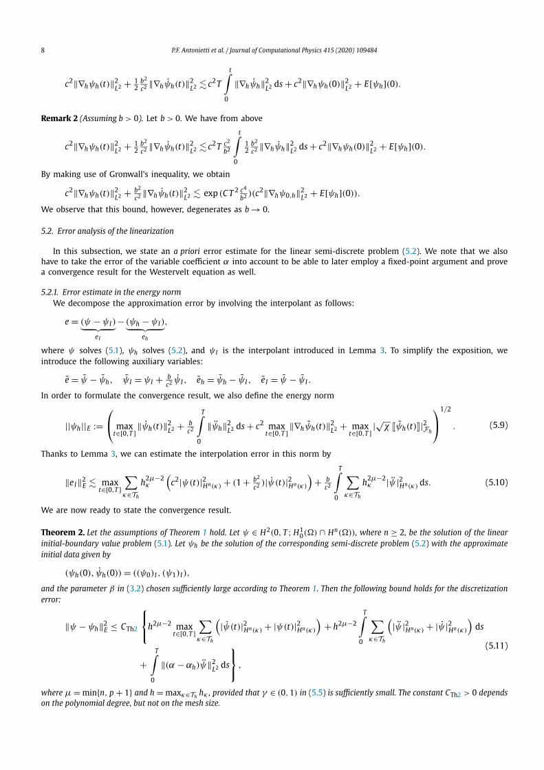
8 P.F. Antonietti et al. / Journal of Computational Physics 415 (2020) 109484

c2‖∇hψh(t)‖2L2 + 1

2b2

c2 ‖∇hψh(t)‖2L2 c2T

t∫0

‖∇hψh‖2L2 ds + c2‖∇hψh(0)‖2

L2 + E[ψh](0).

Remark 2 (Assuming b > 0). Let b > 0. We have from above

c2‖∇hψh(t)‖2L2 + 1

2b2

c2 ‖∇hψh(t)‖2L2 c2T c2

b2

t∫0

12

b2

c2 ‖∇hψh‖2L2 ds + c2‖∇hψh(0)‖2

L2 + E[ψh](0).

By making use of Gronwall’s inequality, we obtain

c2‖∇hψh(t)‖2L2 + b2

c2 ‖∇hψh(t)‖2L2 exp (C T 2 c4

b2 )(c2‖∇hψ0,h‖2L2 + E[ψh](0)).

We observe that this bound, however, degenerates as b → 0.

5.2. Error analysis of the linearization

In this subsection, we state an a priori error estimate for the linear semi-discrete problem (5.2). We note that we also have to take the error of the variable coefficient α into account to be able to later employ a fixed-point argument and prove a convergence result for the Westervelt equation as well.

5.2.1. Error estimate in the energy normWe decompose the approximation error by involving the interpolant as follows:

e = (ψ − ψI )︸ ︷︷ ︸eI

− (ψh − ψI )︸ ︷︷ ︸eh

,

where ψ solves (5.1), ψh solves (5.2), and ψI is the interpolant introduced in Lemma 3. To simplify the exposition, we introduce the following auxiliary variables:

e = ψ − ψh, ψI = ψI + bc2 ψI , eh = ψh − ψI , e I = ψ − ψI .

In order to formulate the convergence result, we also define the energy norm

||ψh||E :=⎛⎝ max

t∈[0,T ] ‖ψh(t)‖2L2 + b

c2

T∫0

‖ψh‖2L2 ds + c2 max

t∈[0,T ] ‖∇hψh(t)‖2L2 + max

t∈[0,T ] |√

χ ψh(t)|2Fh

⎞⎠

1/2

. (5.9)

Thanks to Lemma 3, we can estimate the interpolation error in this norm by

‖eI‖2E max

t∈[0,T ]∑κ∈Th

h2μ−2κ

(c2|ψ(t)|2Hn(κ) + (1 + b2

c2 )|ψ(t)|2Hn(κ)

)+ b

c2

T∫0

∑κ∈Th

h2μ−2κ |ψ |2Hn(κ) ds. (5.10)

We are now ready to state the convergence result.

Theorem 2. Let the assumptions of Theorem 1 hold. Let ψ ∈ H2(0, T ; H10() ∩ Hn()), where n ≥ 2, be the solution of the linear

initial-boundary value problem (5.1). Let ψh be the solution of the corresponding semi-discrete problem (5.2) with the approximate initial data given by

(ψh(0), ψh(0)) = ((ψ0)I , (ψ1)I ),

and the parameter β in (3.2) chosen sufficiently large according to Theorem 1. Then the following bound holds for the discretization error:

‖ψ − ψh‖2E ≤ CTh2

⎧⎨⎩h2μ−2 max

t∈[0,T ]∑κ∈Th

(|ψ(t)|2Hn(κ) + |ψ(t)|2Hn(κ)

)+ h2μ−2

T∫0

∑κ∈Th

(|ψ |2Hn(κ) + |ψ |2Hn(κ)

)ds

+T∫

0

‖(α − αh)ψ‖2L2 ds

⎫⎬⎭ ,

(5.11)

where μ = minn, p + 1 and h = maxκ∈Th hκ , provided that γ ∈ (0, 1) in (5.5) is sufficiently small. The constant CTh2 > 0 depends on the polynomial degree, but not on the mesh size.

P.F. Antonietti et al. / Journal of Computational Physics 415 (2020) 109484 9

The proof of this auxiliary result is given in the appendix. Now we proceed directly with the analysis of the nonlinear model.

6. Analysis of the nonlinear model

Our next aim is to analyze the semi-discretization of the Westervelt equation given by (4.4). To this end, we will rely on our results for the linearized problem together with a fixed-point argument. We point out, however, that we have to restrict ourselves to the case b > 0. The reason for this is that we will need a uniform in h bound for ‖ψh‖L2 L2 . Such a bound follows from ψh being bounded in the energy norm, defined in (5.9), only if b > 0.

Theorem 3. Let c > 0, b > 0, and k ∈ R. Let the final time T > 0 be given and assume that the initial-boundary value problem (2.2)for the Westervelt equation has a solution

ψ ∈ H2(0, T ; H10() ∩ Hn()), where n > 1 + d/2,

for which it holds that

0 < α0 ≤ 1 − 2kψ ≤ α1 in × [0, T ]for some α0 , α1 > 0. Assume that the polynomial degree p ≥ 2 and that the approximate initial conditions are given by

(ψh(0), ψh(0)) = ((ψ0)I , (ψ1)I ). (6.1)

Then for sufficiently small h = maxκ∈Th

hκ and

M(ψ) = maxt∈[0,T ] |ψ(t)|2Hn + max

t∈[0,T ] |ψ(t)|2Hn + maxt∈[0,T ] ‖ψ(t)‖2

L∞ +T∫

0

(|ψ |2Hn + ‖ψ‖2L∞ + |ψ |2Hn )ds,

the corresponding semi-discrete problem (4.4) for the Westervelt equation has a unique solution ψh ∈ H2(0, T ; Vh) that satisfies the following error bound:

||ψ − ψh||2E ≤ CTh 3 h2μ−2∑κ∈Th

⎧⎨⎩ max

t∈[0,T ]

(|ψ(t)|2Hn(κ) + |ψ(t)|2Hnκ)

)+

T∫0

(|ψ |2Hn(κ) + |ψ |2Hn(κ)

)ds

⎫⎬⎭ ,

with μ = minn, p + 1, provided that the parameter β in (3.2) is sufficiently large. The constant CTh3 > 0 depends on M(ψ) and on the polynomial degree, but not on the mesh size.

Proof. We conduct the proof by employing the Banach fixed-point theorem. Therefore, we first need to define a fixed-point map. We begin by introducing the ball

Bh =

wh ∈ H2(0, T ; Vh) : ||ψ − wh||2E ≤ CTh3 h2μ−2∑κ∈Th

maxt∈[0,T ]Eκ [ψ](t) (wh(0), wh(0)) = (ψ0,h,ψ1,h)

⎫⎬⎭ ,

where we have used the notation

Eκ [ψ](t) =|ψ(t)|2Hn(κ) + |ψ(t)|2Hn(κ) +t∫

0

(|ψ |2Hn(κ) + |ψ |2Hn(κ)

)ds.

The constant CTh3 > 0 will be made precise below.

Step 1: Defining the fixed-point map.For wh ∈ Bh , we then define the operator J : wh → ψh , where ψh solves⎧⎨

⎩((1 − 2kwh)ψh, vh)L2 + ah(ψh, vh) = 0 for all vh ∈ Vh, t ∈ (0, T ),

(ψh(0), ψh(0)) = (ψ0,h,ψ1,h).

(6.2)

The operator J is well-defined thanks to the well-posedness result of Theorem 1, whose assumptions we verify below. We note that the set Bh is non-empty when CTh3 ≥ CTh2 because the solution of the linear problem (5.2) with αh = α belongs to it. Moreover, Bh is closed with respect to topology induced by ‖ · ‖E .

10 P.F. Antonietti et al. / Journal of Computational Physics 415 (2020) 109484

Step 2: The self-mapping property.We next want to verify that J (Bh) ⊂ Bh . Let wh ∈ Bh . To show that ψh = J (wh) ∈ Bh , we rely on Theorems 1 and 2, which guarantee stability and convergence for the linearized problem. We choose the variable coefficient in the linear model to be αh = 1 − 2kwh and check that all the assumptions of these theorems are satisfied. In particular, we have to justify the non-degeneracy assumption (5.3) and the smallness of αh/αh in (5.5).

We already know that αh = 1 − 2kwh ∈ H1(0, T ; Vh). We next rely on the inverse estimate given in Lemma 1 and properties of the interpolant stated in Lemma 3 to verify the non-degeneracy assumption (5.3) on αh .

The coefficient αh does not degenerate. Fix t ∈ [0, T ]. We can pick an element κ ∈ Th , such that

maxx∈

|wh(x, t)| = maxx∈κ

|wh(x, t)|. (6.3)

By involving the local interpolant and then relying on the inverse estimate, we find that

maxx∈

|wh(x, t)|2 = maxx∈κ

|wh(x, t)|2

triangle ineq. ‖ψI,κ (t) − wh(t)‖2

L∞(κ)+ ‖ψI,κ (t)‖2

L∞(κ)

inverse est. h−d

κ‖ψI,κ (t) − wh(t)‖2

L2(κ)+ ‖ψI,κ (t)‖2

L∞(κ)

triangle ineq. h−d

κ

(‖ψI,κ (t) − ψ(t)‖2

L2(κ)+ ‖ψ(t) − wh(t)‖2

L2(κ)

)+ ‖ψI,κ (t)‖2

L∞(κ).

(6.4)

We can estimate the last three terms on the right-hand side of (6.4) by employing the stability and approximation properties of the interpolant, and the fact that wh ∈ Bh . By doing so, we obtain

maxx∈

|wh(x, t)|2 h2μ−dκ

|ψ(t)|2Hs(κ)+ h−d

κh2μ−d CTh3

∑κ∈Th

maxt∈[0,T ]Eκ [ψ](t) + ‖ψI,κ (t)‖2

L∞(κ)

h2μ−d|ψ(t)|2Hs() + CTh3

(h

hκ

)d

h2μ−2−d∑κ∈Th

maxt∈[0,T ]Eκ [ψ](t) + ‖ψI,κ (t)‖2

L∞(κ),

recalling that due to our assumptions, we have μ = minn, p + 1 > 1 + d/2. By using the L∞ stability of the interpolant and the assumption on quasi-uniformity of the mesh, we infer

maxx∈

|wh(x, t)|2 ≤ C1M(ψ)(

h2μ−d + CTh3(M(ψ))h2μ−2−d + 1)

:= m (6.5)

for every t ∈ [0, T ], where the constant C1 > 0 above does not depend on the mesh size. We refer to (6.8) below for the exact form of CTh3(M(ψ)). By taking the maximum over t ∈ [0, T ] in (6.5), we further have

‖wh‖C(×[0,T ]) ≤ √m.

We then choose M(ψ) and h sufficiently small so that

0 < α0 ≤ 1 − 2|k|√m ≤ αh = 1 − 2kwh ≤ 1 + 2|k|√m ≤ α1

in × [0, T ].The quotient αh/αh is sufficiently small. The assumption on αh/αh in Theorems 1 and 2 can be verified as follows:∥∥∥∥ αh

αh

∥∥∥∥L1 L∞

=∥∥∥∥ −2kwh

1 − 2kwh

∥∥∥∥L1 L∞

≤ 2|k|1 − 2|k|√m

‖wh‖L1 L∞

≤ 2|k|1 − 2|k|√m

√T ‖wh‖L2 L∞ .

We can bound ‖wh‖L2 L∞ in a similar fashion as (6.3)–(6.5) by relying on the interpolant and inverse estimates. Note, however that this bound would degenerate if b → 0 because by the definition of the energy norm (5.9) we have

‖wh‖L2 L2 ≤ c2

b‖wh‖E . (6.6)

Therefore, we find

T∫0

maxx∈

|wh(s)|2 ds h2μ−d

T∫0

|ψ(s)|2Hs() ds + c4

b2CTh3h2μ−2−d

∑κ∈Th

maxt∈[0,T ]Eκ [ψ](t)+

T∫0

‖ψI,κ (s)‖2L∞(κ)

ds,

P.F. Antonietti et al. / Journal of Computational Physics 415 (2020) 109484 11

from which it follows that

T∫0

maxx∈

|wh(s)|2 ds ≤ C2m, (6.7)

where the constant C2 > 0 does not depend on the mesh size, but it degenerates if b tends to zero. Therefore, for Theorem 2to hold, we need that

γ := 2|k|1 − 2|k|√m

√T C2m

is sufficiently small, which we can achieve by decreasing M(ψ) and h.Choosing the constant CTh3 so that J is a self-mapping. We have therefore verified all the assumptions of Theorems 1 and 2.

On account of Theorem 2 and the resulting error estimate (5.11), we conclude that problem (6.2) has a unique solution ψh ∈ C2([0, T ]; Vh) that satisfies

||ψ − ψh||2E ≤ CTh2

⎛⎝h2μ−2

∑κ∈Th

maxt∈[0,T ]Eκ [ψ](t) + max

t∈[0,T ] ‖α(t) − αh(t)‖2L2

T∫0

‖ψ‖2L∞() ds

⎞⎠ .

Noting that the error in α can be estimated according to

maxt∈[0,T ] ‖α(t) − αh(t)‖2

L2 = maxt∈[0,T ] ‖2kψ(t) − 2kwh(t)‖2

L2

≤4k2CTh3 h2μ−2∑κ∈Th

maxt∈[0,T ]Eκ [ψ](t),

since wh ∈ Bh , we obtain

||ψ − ψh||2E ≤ CTh2 (1 + 4k2CTh3M(ψ))h2μ−2∑κ∈Th

maxt∈[0,T ]Eκ [ψ](t).

For sufficiently small M(ψ) such that 1 − 4k2CTh2M(ψ) > 0, we can choose CTh3 as

CTh3 := CTh2

1 − 4k2CTh2M(ψ). (6.8)

This choice of the constant CTh3 implies that

||ψ − ψh||2E ≤ CTh3h2μ−2∑κ∈Th

maxt∈[0,T ]Eκ [ψ](t);

in other words, ψh ∈ Bh .

Step 3: Contractivity.To prove that the operator J is strictly contractive, take w(1)

h , w(2)

h ∈ Bh and set ψ(1)

h = J (w(1)

h ), ψ(2)

h = J (w(2)

h ) ∈ Bh . Denote Wh = w(1)

h − w(2)

h . Then the difference h = ψ(1)

h − ψ(2)

h satisfies the problem

((1 − 2kw(1)

h )h, vh)L2 + ah(h, vh) = (2k Wh ψ(2)

h , vh)L2 , vh ∈ Vh (6.9)

for all time, with zero initial data. This equation corresponds to equation (A.4) satisfied by the approximation error in the proof of Theorem 2. Therefore, testing (6.9) with ˙

h and proceeding analogously to the proof of Theorem 2 results in the estimate

||h||2E 4k2(1 + bc2 )α−1

0

⎧⎨⎩

T∫0

‖ψ(2)

h ‖2L∞() ds

⎫⎬⎭ max

t∈[0,T ] |Wh(t)|2L2 .

This inequality then corresponds to estimate (A.9) in the proof of Theorem 2 if we formally set the interpolant error to zero. We further have

||h||2E 4k2(1 + bc2 )α−1

0

⎧⎨⎩

T∫0

‖ψ(2)

h ‖2L∞() ds

⎫⎬⎭ ||Wh||2E . (6.10)

12 P.F. Antonietti et al. / Journal of Computational Physics 415 (2020) 109484

We can bound ‖ψ(2)

h ‖2L2 L∞ by proceeding in the same way as in (6.6)–(6.7). This term can thus be made sufficiently small

by reducing M(ψ) and h. From estimate (6.10), we then conclude that J is contractive for sufficiently small M(ψ) and h.On account of Banach’s contraction principle, the mapping J has a unique fixed-point ψh = J (ψh) ∈ Bh , which is, in

turn, the unique solution of the nonlinear semi-discrete problem (4.4) with approximate initial data (6.1).

7. Computational DG approach for nonlinear sound waves

Starting from the semi-discrete equation (4.4), this section describes the numerical treatment and solution process involving the assembly of an equation in matrix-vector form and the time-integration scheme that is used. Discontin-uous Galerkin approaches for nonlinear acoustic waves based on a first-order conservation system are investigated in, e.g., [38,56,57].

7.1. The matrix form of the semi-discrete problem

For the purpose of carrying out our numerical experiments, we consider here a more general case than before of having either a non-zero source term or inhomogeneous Dirichlet boundary conditions. We present the numerical treatment of the latter case; the simpler case of having a non-zero source term f can be treated in an analogous manner.

Let ψ = g on D = ∂, where the function g is assumed to be sufficiently smooth on D, compatible with initial data. The Dirichlet conditions are imposed in a weak sense; see [19, Chapter 4, Section 4.2.2] for a detailed explanation. Therefore, in our semi-discrete weak form, the following terms arise additionally on the right-hand side:∫

D

−c2 g(∇v · n

)dS +

∫D

χ g v dS,

where, analogously to before, we have used the auxiliary notation g = g + bc2 g .

The semi-discrete form of (4.4) then reads as

Mψ +(

K − D − D + P)

(ψ + bc2 ψ) − T [·, ψ, ψ] = w, (7.1)

where M denotes the standard mass matrix and K the stiffness matrix. In addition, we assemble the nonlinearity tensor T , the DG penalty matrix P, the DG jump matrix D, and the Dirichlet data vector w. Furthermore, we introduce the shorthand notation A := K − D − D + P.

We therefore have a second-order system of ordinary differential equations with a nonlinear term on the right-hand side, which now remains to be solved by a suitable time-integration scheme. Herein the initial data approximations (ψh(0), ψh(0)) = (ψ0,h, ψ1,h) ∈ Vh × Vh are represented in the finite element basis via the coefficient vectors ψ

0and ψ

1such that for the ODE-system we have ψ(0) = ψ

0and ψ(0) = ψ

1.

7.2. Time integration

In order to integrate the system of ordinary differential equations (7.1) in time, we employ either the Newmark scheme or the Newmark-type Generalized-α method; we refer to [31,36] for a similar strategy. The nonlinear term is resolved via a fixed-point iteration during the solving stage of the predictor-corrector scheme. The termination criterion that checks the relative change of the solution-vector between iteration steps is employed. In the experiments with realistic physical data, where we observe the nonlinear steepening of the wave front in our computational domain, we choose the Generalized-αscheme because it allows to add targeted numerical damping to the higher modes and subdue Gibbs oscillations.

The algorithm for conducting the timestep n → n + 1 within the Generalized-α scheme is given in the following. It involves ψn, ψn

, and ψnas the approximations of ψ, ψ , and ψ at time level tn = nt , where t is a suitable timestep. The

so-called effective mass matrix

M∗ = (1 − αm)M + (1 − α f )γnmtb

c2A + (1 − α f )βnmt2A

and the intermediate time tn+1,α := (1 − α f )tn+1 + α f tn are also used within the time-stepping algorithm.Predictor step:

ψpred

= ψn + tψn + t2

2(1 − 2βnm)ψ

n, ψ

pred,α= (1 − α f )ψpred

+ α f ψn

ψpred

= ψn + (1 − γnm)tψ

n, ψ

pred,α= (1 − α f )ψpred

+ α f ψn

Iteration over κ = 1, 2, 3, ..., κmax with ψ1= ψn, ψ

1= ψ

n, ψ

1= ψ

n

P.F. Antonietti et al. / Journal of Computational Physics 415 (2020) 109484 13

Table 1Numerical parameters used in the experiments.

Test case 1 Test case 2 Test case 3 Test case 4

Newmark scheme βnm = 0.25γnm = 0.5

βnm = 4/9γnm = 5/6

βnm = 4/9γnm = 5/6

βnm = 4/9γnm = 5/6

Generalized-α scheme αm = 0α f = 0

αm = 0α f = 1/3

DG penalty β = 10 β = 10 β = 250 β = 1750

α-Combinations

ψκ,α

= (1 − α f )ψκ+ α f ψ

n

ψκ,α

= (1 − α f )ψκ+ α f ψ

n

ψκ,α

= (1 − αm)ψκ

+ αmψn

Solve algebraic system

M∗ψκ+1

= w(tn+1,α) − αmMψn − b

c2Aψ

pred,α

− Aψpred,α

+ T[·, ψ

κ,α, ψ

κ,α

]

Corrector step:

ψκ+1

= ψpred

+ βnmt2ψκ+1

ψκ+1

= ψpred

+ γnmtψκ+1

Check termination criterion:

If‖ψ

κ+1− ψ

κ‖

‖ψκ+1

‖ < TOL, set

⎧⎪⎪⎨⎪⎪⎩

ψn+1 = ψκ+1

ψn+1 = ψ

κ+1

ψn+1 = ψ

κ+1

and break iterationend iterationThe numerical parameters that are used in the forthcoming experiments can be found in Table 1. The physical and

discretization parameters for each experiment are given below in their respective sections.In Table 1, the values βnm and γnm denote the parameters in the Newmark scheme given in the formulas above. The

numbers αm and α f are the additional parameters in the Generalized-α scheme. TOL is the relative tolerance in the termi-nation criterion of the fixed-point-iteration, κmax stands for the maximum number of iterations after which the algorithm should abort. Those parameters were chosen to be TOL = 10−5 and κmax = 100 throughout all experiments. Finally, β is the DG-penalty term introduced in (3.2).

8. Numerical results

In this section, we perform numerical experiments to illustrate our theoretical findings. The first two numerical tests are conducted in a two-dimensional computational setting based on a MATLAB implementation. The third and fourth, three-dimensional experiments were implemented in SPEED—a parallel, high-order spectral finite-element FORTRAN code [40].

8.1. Test case 1: exact solution known

In our first example, we simulate the Westervelt equation (2.1) with a given source term f on the right hand side, which we choose as

f =[

16π2(c2 − 1) sin(4πt) + 64π3b cos(4πt)]

sin(4πx) +[

64π3k sin(4πt) cos(4πt)]

sin(4πx)2.

In this way, the exact solution is given by ψ = sin(4πx) sin(4πt), which we use in the error analysis. In this numerical experiment, all the physical quantities involved are assumed to be dimensionless. Our computational domain is given by the rectangle = (0, 1) × (0, 23

√3). We tessellate it with Nelem polygonal elements in two ways: a regular hexagonal

pattern and a random way using polygons with different number of edges each; see Fig. 1 for exemplary depictions of the resulting grids. The ratio of domain length and width is chosen such that the regular tessellation bears the same element shapes in the interior as well as (exactly halfed elements) on all four sides yielding control over the mesh quality. The initial conditions and Dirichlet boundary data are set to correspond to the values of ψ at time zero and on the boundary, respectively.

We choose the coefficients in the equation to be c = 1, b = 10−5, βa = 10−4, and the mass density is ρ = 1. The time-discretization is conducted with final time T = 0.8 and the Newmark scheme, where the timestep size is always adapted in such a way, that the time-discretization error does not dominate in Fig. 2 and the convergence with respect to the number of elements can be observed.

14 P.F. Antonietti et al. / Journal of Computational Physics 415 (2020) 109484

Fig. 1. Computational domain with exemplary polygonal grids. (left) regular hexagonal grid, (right) grid with arbitrary polygonal structure and highlighting of a few exemplary “small” edges, making the grid only suitable under the weaker assumptions discussed in Remark 1.

Fig. 2. L2 and |∇h(·)|L2 errors of ψh at final time for four sequentially refined polygonal meshes and second- and third-order polynomials, comparing a sequence of regular polygonal grids (reg.) with a sequence of irregular ones (rand.).

We perform this experiment on a sequence of regular grids that satisfy our mesh assumptions and on an unstructured grid which might not; see Fig. 1. Such unstructured meshes satisfy the weaker assumptions discussed in Remark 1, which is why we want to test if we still observe the same order of convergence when using them.

Fig. 2 displays convergence results for five sequentially refined polygonal meshes, where we have employed polynomials of degree p = 2 and p = 3. As a reference, on the five levels the unstructured grid consists out of 281, 827, 1828, 2998, and 4727 elements, respectively. As expected in practice for DG methods, the L2-error of the acoustic velocity potential converges with the order hp+1; see, e.g., [28].

8.2. Test case 2: exact solution unknown

Our second example features a more realistic setting. The computational domain is chosen to be a rectangle with dimen-sions H = 0.02 m and L = 3√

3· 0.02 m; see Fig. 3 left. The physical parameters are now set to

c = 1500 m/s, b = 6 × 10−9 m2/s, βa = 7, and ρ = 1000 kg/m3.

The time horizon is T = 2.4 × 10−5 s, resolved by a step size of dt = 2 × 10−9 s. Instead of a non-zero source term f , we employ inhomogeneous Dirichlet conditions. The excitation signal is given in the form g(x, y, t) = g(s)(x, y) · g(t)(t). Herein the temporal part responsible for the initialization of the wave oscillations is given by

g(t)(t) =⎧⎨⎩

(f t2

)2A sin(ωt), t < 2

f s,

A sin(ωt), t ≥ 2f s,

P.F. Antonietti et al. / Journal of Computational Physics 415 (2020) 109484 15

Fig. 3. (left) Computational domain with exemplary polygonal grid. The left boundary is the excitation part, where the Dirichlet data g is non-zero. At remaining boundary parts homogeneous Dirichlet data are imposed. The blue line is the axis of symmetry over which the solution is evaluated on the right. (right) Computed acoustic pressure field uh = ρψh over the horizontal axis of symmetry of the channel at final time T of a simulation with increased amplitude A = 0.0175 m2/s2, plotted together with the pressure wave obtain by solving the linear damped wave equation with same boundary and initial data. (For interpretation of the colors in the figure(s), the reader is referred to the web version of this article.)

while the spatial part is given by a mollifier-type function in order to get a spatially smooth transition between the inho-mogeneous excitation and the homogeneous remaining boundary data. In particular, we have

g(s)(x, y) =

⎧⎪⎪⎪⎪⎪⎪⎪⎪⎪⎪⎪⎪⎪⎨⎪⎪⎪⎪⎪⎪⎪⎪⎪⎪⎪⎪⎪⎩

0, x = 0 m, y = 0 m

exp

(1 − 1

1−∣∣∣ 1

0.005 (y−0.005)

∣∣∣2

), x = 0 m,0 m < y < 0.005 m

1, x = 0 m,0.005 m ≤ y ≤ 0.015 m

exp

(1 − 1

1−∣∣∣ 1

0.005 (y−0.015)

∣∣∣2

), x = 0 m,0.015 m < y < 0.02 m

0, x = 0 m, y = 0.02 m

0, 0 m < x

We therefore employ a spatially smooth, temporally modulated sinusoidal excitation with driving frequency f = 210 kHzand amplitude A = 0.01 m2/s2, where ω denotes the angular frequency ω = 2π f . Fig. 3 displays a plot of the acoustic pressure uh = ρψh along the horizontal axis of symmetry of the channel at final time T . To better observe the nonlinear steepening, the figure also contains a pressure wave obtained by solving the linear damped wave equation (i.e., Westervelt’s equation with k = 0).

We next want to analyze the behavior of the numerical solution with respect to h- and p-refinement. However, in this more realistic setting an exact solution is unknown. Therefore, instead of tracking the deviation from a given solution, we track a given quantity of interest. Here we choose to compute

Q (ψh) := ‖ψh‖L∞(0,T ;L2()), (8.1)

on different discretization levels. We note that

Q (ψ) − ‖ψh − ψ‖L∞(0,T ;L2()) ≤ Q (ψh) ≤ Q (ψ) + ‖ψh − ψ‖L∞(0,T ;L2()),

and so we expect that, for p fixed, Q (ψh) behaves asymptotically as q1 + q2 · hp+1 for some constants q1 and q2.

h-refinement. We restrict ourselves to structured, quasi-uniform polygonal meshes consisting of Nelem ∈ 220, 312, 420, 544,

684, 840, 1104, 1740, 2664 elements. The polynomial degree is set to p = 3. Values Q (ψh) for these levels of refinement are plotted in Fig. 4 on the left. In order to observe the convergence order, we perform a least-square fit of the (h, Q (ψh))

data pairs. We obtain a fitted curve

Q f (h) = q1 + q2 · h4,

where q1 and q2 are subject to the least-square fit. The fitted curve Q f with optimized parameters reads approximately as

Q f (h) = 1.322735 · 10−4 − 504.613929 · h4

and is plotted in Fig. 4 on the left as well. As expected, we observe O (hp+1) convergence. The extrapolated value for the quantity of interest Q f (0) evaluates to 1.322735 · 10−4.

16 P.F. Antonietti et al. / Journal of Computational Physics 415 (2020) 109484

Fig. 4. (left) The quantity of interest Q (ψh) = ‖ψh‖L∞(0,T ;L2()) computed on a sequence of polygonal meshes with third-order polynomials and a least-

square fitted extrapolation-curve of order h4. (right) Deviation of the computed quantity of interest Q (ψh) from a reference value as a function of p on a fixed mesh.

p-refinement. We also perform a refinement analysis of the quantity of interest with respect to the polynomial degree. Here we choose a fixed mesh with Nelem = 312 elements and successively increase the polynomial degree p ∈ 1, 2, ..., 7, where it should be mentioned that even though our theory holds for p ≥ 2, the case p = 1 yields a similar result as well. The deviations of the resulting quantities from a reference value are plotted in Fig. 4 on the right. As the reference, we choose the extrapolated value of the h-refinement with degree p = 4. For p = 7, the quantity of interest evaluates to 1.322730 ·10−4

with the deviation from the extrapolated reference value below 7.6 · 10−5 %.

8.3. Test case 3: a three-dimensional example

Our third example is performed in a three dimensional setting, where we use the discontinuous Galerkin approach in a hybrid way. Fig. 5 shows an image of the computational geometry consisting of six different material blocks. The blocks differ in all relevant material parameters, given in Table 2. This example is motivated by nonlinear sound propagation in inhomogeneous media. These types of computational settings often arise in medical ultrasound when the sound waves propagate through human body with varying speed of sound and other medium parameters; see, for example, [46]. We, therefore, solve here Westervelt’s equation

(1 − 2k(x)ψ)ψ − div(c2(x)∇ψ) − div(b(x)∇ψ) = 0

with coefficients in L∞(). The pressure is then computed via u = (x)ψt , where the mass density is now as well in L∞(). The stabilization function has the form

χ|F =

⎧⎪⎪⎪⎪⎨⎪⎪⎪⎪⎩

β maxκ∈κ+,κ−

c2|κp2

hκfor all F ∈ F i

h, F ⊂ ∂κ+ ∩ ∂κ−,

βc2|κp2

hκfor all F ∈ Fb

h , F ⊂ ∂κ.

To save computational power, the blocks are meshed and discretized individually via conforming spectral elements within each block, while the discontinuous Galerkin approach deals with the non-matching grids on the interfaces.

Setup of the experiment. Block 1 has a width and length of 0.025 m and a height of 0.01 m; see Fig. 5. On its bottom surface, the wave excitation takes place. We use an excitation signal in the form of a Dirichlet condition similarly to Section 8.2. The four walls of the block are equipped with homogeneous Neumann/symmetry boundary conditions, its top surface with a homogeneous Dirichlet condition, except at the interfaces to the blocks 2 to 5. Those are truncated four-sided pyramids which are aligned in a regular way between blocks 1 and 6, each with a height of 0.01 m and homogeneous Dirichlet conditions on its four walls. Block 6, with a height of 0.04 m and the remaining measures as for Block 1, covers the upper part of the geometry, again equipped with homogeneous Neumann/symmetry conditions on its four sides and homogeneous Dirichlet conditions at top and bottom, except for the interfaces with the blocks 2 to 5.

The excitation signal is given by

g(t, x, y, z) = g(t)(t) =⎧⎨⎩

(f t2

)2A sin(ωt), t < 2

f s

0, t ≥ 2f s;

P.F. Antonietti et al. / Journal of Computational Physics 415 (2020) 109484 17

Fig. 5. Test case 3: Computational domain with six different material blocks. Each block has its own material parameters, mesh, and ansatz space. Interface coupling is done via the DG approach.

Table 2Physical parameters of different material blocks.

Material block 1 • 2 • 3 • 4 • 5 • 6 •c [m/s] 1500 1000 1000 3000 750 1500b

[m2/s

]6 × 10−9 4 × 10−9 4 × 10−2 4 × 10−9 6 × 10−9 6 × 10−9

βa 5 4 4 7 4 5ρ

[kg/m3

]1000 1250 1250 2000 1500 1000

Fig. 6. Iso-volumina at time steps (left) 12000 (middle) 19000 (right) 24600 of the highest acoustic pressure amplitudes (in absolute value) uh = ρψh

during wave propagation through the four connecting channels of the computational domain. The orientation of the images is the same as in Fig. 5.

i.e., by a cut-off pulse-version of the continuous excitation signal used before. We use such a signal here in order to avoid interference within the block 1 originating from reflections off the walls between the interfaces to blocks 2 to 5. Amplitude and frequency are chosen as before. For the time discretization again the Generalized-α method is used with the final time T = 2.217 · 10−5 s, resolved with a step size of t = 10−9 s.

Fig. 6 shows snapshots of the solution computed with p = 2 on 260730 elements. We observe iso-volumina of the highest acoustic pressure amplitudes at different time steps which show how the wave propagates through the four separate channels connecting the base block with the top block. Especially the deviations in the speed of sound are visible as the

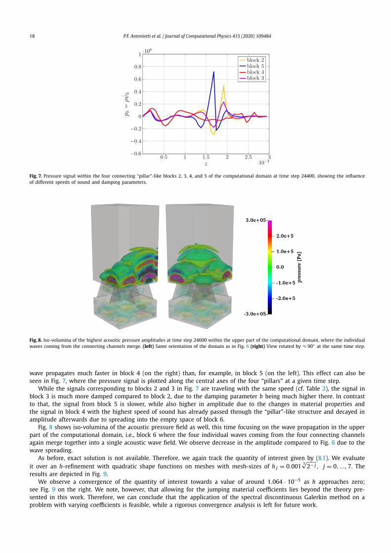
18 P.F. Antonietti et al. / Journal of Computational Physics 415 (2020) 109484

Fig. 7. Pressure signal within the four connecting “pillar”-like blocks 2, 3, 4, and 5 of the computational domain at time step 24400, showing the influence of different speeds of sound and damping parameters.

Fig. 8. Iso-volumina of the highest acoustic pressure amplitudes at time step 24600 within the upper part of the computational domain, where the individual waves coming from the connecting channels merge. (left) Same orientation of the domain as in Fig. 6 (right) View rotated by ≈ 90 at the same time step.

wave propagates much faster in block 4 (on the right) than, for example, in block 5 (on the left). This effect can also be seen in Fig. 7, where the pressure signal is plotted along the central axes of the four “pillars” at a given time step.

While the signals corresponding to blocks 2 and 3 in Fig. 7 are traveling with the same speed (cf. Table 2), the signal in block 3 is much more damped compared to block 2, due to the damping parameter b being much higher there. In contrast to that, the signal from block 5 is slower, while also higher in amplitude due to the changes in material properties and the signal in block 4 with the highest speed of sound has already passed through the “pillar”-like structure and decayed in amplitude afterwards due to spreading into the empty space of block 6.

Fig. 8 shows iso-volumina of the acoustic pressure field as well, this time focusing on the wave propagation in the upper part of the computational domain, i.e., block 6 where the four individual waves coming from the four connecting channels again merge together into a single acoustic wave field. We observe decrease in the amplitude compared to Fig. 6 due to the wave spreading.

As before, exact solution is not available. Therefore, we again track the quantity of interest given by (8.1). We evaluate it over an h-refinement with quadratic shape functions on meshes with mesh-sizes of h j = 0.001

3√2− j, j = 0, ..., 7. The

results are depicted in Fig. 9.We observe a convergence of the quantity of interest towards a value of around 1.064 · 10−5 as h approaches zero;

see Fig. 9 on the right. We note, however, that allowing for the jumping material coefficients lies beyond the theory pre-sented in this work. Therefore, we can conclude that the application of the spectral discontinuous Galerkin method on a problem with varying coefficients is feasible, while a rigorous convergence analysis is left for future work.

P.F. Antonietti et al. / Journal of Computational Physics 415 (2020) 109484 19

Fig. 9. Quantity of interest over an h-refinement with quadratic shape functions. (left) L2() norm of the numerical solution over the course of time for all tested levels of refinement (right) Respective L∞(0, T ; L2())-norm results on all 8 mesh levels in order to observe convergence.

Fig. 10. (left) Acoustic domain consisting out of different layers of air with different material properties. (right) Topographic profile of the mountain range below the acoustic layers.

8.4. Test case 4: wave scattering

Our final example deals on a larger spatial scale, where seismic events take place. In particular, we are motivated by nonlinear effects that can be observed in seismic wave propagation [27,45]. In this experiment, the acoustic medium is a rectangularly cut-out block of air above a mountain-like range. On the top-surface of the acoustic domain, a wave is excited vertically and is traveling towards the mountain’s surface where it gets reflected. On its way towards the mountain’s surface, the wave travels through different layers of the acoustic medium bearing different material properties.

In the applicational context, these could be layers of air-currents of different temperature and hence varying density ρ and speed of sound c2. The coupling between those layers is again performed by employing the discontinuous-Galerkin approach in a hybrid way to couple non-conforming meshes. This feature is especially useful in the context of locally refined grids. In the present case, this is done by resolving the layers with more complex dynamics closer to the reflecting mountain surface finer than the most upper air-layer, resulting in non-conforming mesh-interfaces between the layers.

Fig. 10 (left) shows an image of the computational domain highlighting the different layers in use. The bottom and middle layer have a height of 2000 m each. The top layer has a minimal thickness of 3000 m. Fig. 10 (right) shows the topographic profile of the mountain range below the air layers. The depicted area has a width and length of 11520 mand is located on the earth’s surface with mid-point at 11.51855 E, 48.07305 N (Munich-area, Germany, with the Alps in the south). The elevation model was constructed from data in the Digital Elevation Database (http://srtm .csi .cgiar.org/). The altitudes have been smoothed and are exaggerated by a factor of 40 and normalized to a minimum of 0 m to create a more dynamic profile.

20 P.F. Antonietti et al. / Journal of Computational Physics 415 (2020) 109484

Table 3Physical parameters of different air layers.

Material block Top layer Mid layer Bottom layer

c [m/s] 351.88 331.30 315.77ρ

[kg/m3

]1.1455 1.2922 1.4224

As for the material parameters, we use the following varying values, see Table 3.The damping and nonlinearity parameters were chosen to be constant with values b = 0.00005 m

2

s , βa = 1.2. The upper surface of the top layer is equipped with a time-varying Dirichlet conditions:

g(t, x, y, z) = e− 1

2

[(x−μxσx

)2+(

y−μyσy

)2]⎧⎪⎪⎪⎪⎪⎨⎪⎪⎪⎪⎪⎩

(f t2

)2A sin(ωt), t < 2

f s⎛⎝1 −

(f(

t− 2f

)2

)2⎞⎠ A sin(ωt), 2

f s ≤ t < 4f s;

0, else,

with parameters: μx = μy = 5760 m, σx = σy = 1000 m, f = 0.1 Hz, A = 0.01 m2/s2. To the lower surface of the bottom block which constitutes the mountain’s surface, we prescribe homogeneous Neumann conditions. On the remaining surfaces encasing the block of air, we employ the Engquist–Majda absorbing boundary conditions, i.e. c∂nψ = −ψt [24], to prevent unphysical reflections traveling back into the domain.

Due to the kilometer scale, the time-horizon of 90 s for this simulation is much larger than in the previous experiments on the centimeter scale. The simulation time is resolved once more by the Generalized-α-method with 30000 timesteps. For spatial discretization, 46516 elements for the top-layer, 82500 elements for the middle layer and 82264 elements for the bottom layer have been used, hence featuring a mesh that is refined more towards the reflection surface, where mesh-coupling between the non-conforming material layers is done via the discontinuous Galerkin method. In this example, the value of the penalty parameter in the DG approach is set to be larger than before. By this we allow for poorly shaped elements at the interfaces, and we do enforce the solution to have no significant jump at the interface between the layers. We note that this does not deteriorate the quality of the solution since the best approximation property of a constrained space having zero jump is in this special case of the same quality as of the unconstrained case. This is due to the fact that our mesh generator starts from a conforming surface mesh for the layers. The value p = 2 is chosen as degree of the basis functions.

Fig. 11 shows the snapshots of the acoustic potential at certain timesteps, such that the reflection of the wave on the mountain’s surface can be observed.

9. Conclusion

We have considered the discretization of the Westervelt’s nonlinear wave equation with strong damping to model sound propagation with losses through homogeneous media. For the space discretization, we proposed a high-order discontinu-ous Galerkin scheme that can support general polygonal/polyhedral meshes. The fully discrete formulation is then obtained based on employing either the Newmark scheme or the Newmark-type Generalized-α method. The nonlinear term is re-solved via a fixed-point iteration during the solving stage of the predictor-corrector scheme.

For the semidiscrete formulation we proved existence, stability and a priori error estimates in a suitable (mesh-dependent) energy norm, under the assumption that the polynomial approximation order p is such that p ≥ 2. To accomplish the the-oretical analysis, preventing the equation from degenerating, and handling the nonlinearity in the model which involves the derivatives in time of the acoustic velocity potential, we made use of the Banach fixed-point theorem combined with a stability and convergence analysis of a linear wave equation with a variable coefficient in front of the second time derivative.

A wide set of two- and three-dimensional numerical experiments validate the theoretical convergence bounds and il-lustrate the practical performance of the proposed method on a practical test case stemming from medical ultra-sound applications and nonlinear seismic waves. Future developments include the extension of the proposed analysis to coupled non-linear elasto-acoustic wave propagation problems, by expanding on the recent results of [1,2] where discontinuous Galerkin and discontinuous Galerkin spectral element methods for the linear elasto-acoustic coupled problem have been proposed. Further research will also cover the extensive testing of the proposed method on a set of challenging test cases stemming from practical applications.

Declaration of competing interest

The authors declare that they have no known competing financial interests or personal relationships that could have appeared to influence the work reported in this paper.

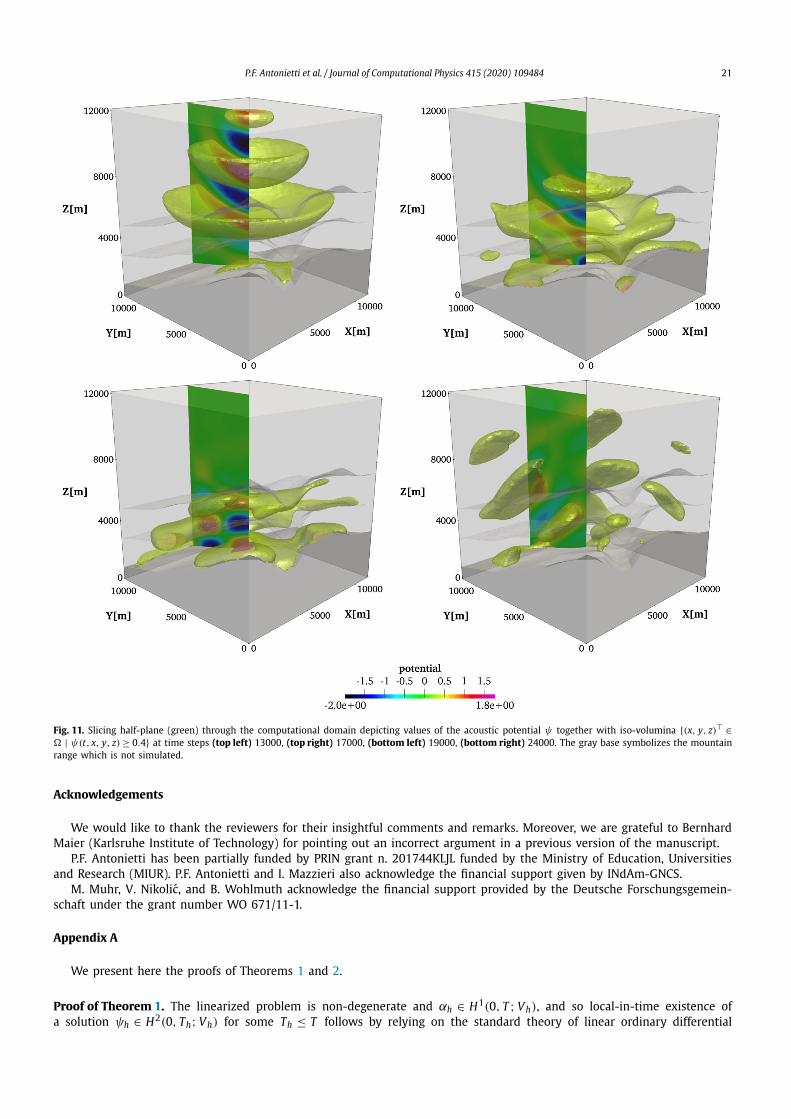
P.F. Antonietti et al. / Journal of Computational Physics 415 (2020) 109484 21

Fig. 11. Slicing half-plane (green) through the computational domain depicting values of the acoustic potential ψ together with iso-volumina (x, y, z) ∈ | ψ(t, x, y, z) ≥ 0.4 at time steps (top left) 13000, (top right) 17000, (bottom left) 19000, (bottom right) 24000. The gray base symbolizes the mountain range which is not simulated.

Acknowledgements

We would like to thank the reviewers for their insightful comments and remarks. Moreover, we are grateful to Bernhard Maier (Karlsruhe Institute of Technology) for pointing out an incorrect argument in a previous version of the manuscript.

P.F. Antonietti has been partially funded by PRIN grant n. 201744KLJL funded by the Ministry of Education, Universities and Research (MIUR). P.F. Antonietti and I. Mazzieri also acknowledge the financial support given by INdAm-GNCS.

M. Muhr, V. Nikolic, and B. Wohlmuth acknowledge the financial support provided by the Deutsche Forschungsgemein-schaft under the grant number WO 671/11-1.

Appendix A

We present here the proofs of Theorems 1 and 2.

Proof of Theorem 1. The linearized problem is non-degenerate and αh ∈ H1(0, T ; Vh), and so local-in-time existence of a solution ψh ∈ H2(0, Th; Vh) for some Th ≤ T follows by relying on the standard theory of linear ordinary differential

22 P.F. Antonietti et al. / Journal of Computational Physics 415 (2020) 109484

equations; cf. [51, Theorem 1.44] and [43, Theorem 4.2]. The upcoming energy estimate will allow us to extend the existence interval to [0, T ].

We next focus on proving stability. In energy analysis of second-order wave equations, the first time derivative of the solution is a natural choice of test function. However, due to the presence of a varying coefficient αh in our case, we would need to additionally test with a suitably scaled second time derivative. We combine these ideas and choose vh = ˙

ψh =ψh + b

c2 ψh as a test function.

Taking vh = ˙ψh in (5.2), integrating over (0, t), where t ≤ Th , and performing integration by parts with respect to time

leads to the identity

t∫0

(αhψh,˙ψh)L2 ds + 1

2 c2‖∇hψh(s)‖2L2

∣∣∣t

0+ 1

2 ‖√χ ψh(s)‖2Fh

∣∣∣t

0

=〈c2∇hψh(s), ψh(s)〉Fh

∣∣∣t

0.

(A.1)

Above, we have made use of the fact that

〈c2∇hψh, ˙ψh〉Fh + 〈ψh, c2∇h

˙ψh〉Fh = d

dt〈c2∇hψh, ψh〉Fh .

We can employ Lemma 4 and inequality (5.4) to obtain

12 c2‖∇hψh‖2

L2 + 12 ‖√χ ψh‖2

Fh− c2〈∇hψh, ψh〉Fh

≥ C1(c2‖∇hψh‖2L2 + ‖√χ ψh‖2

Fh)

for all t ∈ [0, Th], provided that parameter β in (3.2) is sufficiently large. Similarly, we obtain

12 c2‖∇hψh(0)‖2

L2 + ‖√χ ψh(0)‖2Fh

− 〈c2∇hψh(0), ψh(0)〉Fh

≤ C2(c2‖∇hψh(0)‖2L2 + ‖√χ ψh(0)‖2

Fh).

The constants C1, C2 > 0 above are independent of c, b, or the mesh size, but depend on the polynomial degree p. It remains to estimate the αh-term in (A.1). We recall how the auxiliary state ψh is defined in (4.5) and employ integration by parts with respect to time, which results in

t∫0

(αhψh,˙ψh)L2 ds = b

c2

t∫0

‖√αh ψh‖2L2 ds +

t∫0

(αhψh, ψh)L2 ds

=t∫

0

(bc2 ‖√αh ψh‖2

L2 − 12 ‖√

αhψh‖2L2

)ds

+ 12 ‖√

αh(s)ψh(s)‖2L2

∣∣∣t

0.

From here, we can further estimate the last term to obtain

t∫0

(αhψh,˙ψh)L2 ds ≥ b

c2

t∫0

‖√αh ψh‖2L2 ds + 1

2 ‖√αh(s)ψh(s)‖2

L2

∣∣∣t

0

− 12

t∫0

supx∈

∣∣∣∣ αh(x)

αh(x)

∣∣∣∣ · ‖√αhψh‖2L2 ds

≥ bc2

t∫0

‖√αh ψh‖2L2 ds + 1

2 ‖√αh(s)ψh(s)‖2

L2

∣∣∣t

0

− 12 max

s∈[0,Th] ‖√

αh(s)ψh(s)‖2L2

T∫0

supx∈

∣∣∣∣ αh(x)

αh(x)

∣∣∣∣ ds,

where we have additionally employed the fact that t ≤ Th ≤ T in the last step. By combining our previously derived esti-mates, we arrive at

P.F. Antonietti et al. / Journal of Computational Physics 415 (2020) 109484 23

12 ‖√

αh(t)ψh(t)‖2L2 + C1c2‖∇hψh(t)‖2

L2

+ bc2

t∫0

‖√αh ψh‖2L2 ds + C1‖√χ ψh(t)‖2

Fh

≤ 12 ‖√

αh(0)ψh(0)‖2L2 + C2

(c2‖∇hψh(0)‖2

L2 + ‖√χ ψh(0)‖2Fh

)

+ 12 max

s∈[0,Th] ‖√

αh(s)ψh(s)‖2L2

T∫0

supx∈

∣∣∣∣ αh(x)

αh(x)

∣∣∣∣ ds

(A.2)

for all t ∈ [0, Th]. Taking the maximum of the above estimate over [0, Th] then yields

(1 − γ ) maxt∈[0,Th] ‖

√αh(t)ψh(t)‖2

L2 + c2 maxt∈[0,Th] ‖∇hψh(t)‖2

L2

+ bc2

Th∫0

‖√αh ψh‖2L2 ds + max

s∈[0,Th] ‖√

χ ψh(t)‖2Fh

‖√αh(0)ψh(0)‖2

L2 + c2‖∇hψh(0)‖2L2 + ‖√χ ψh(0)‖2

Fh.

(A.3)

Since the right-hand side of (A.3) does not depend on Th , we are allowed to extend the existence interval to [0, T ]; i.e., we can set Th = T . Uniqueness follows by linearity of the problem and the derived stability bound.

Proof of Theorem 2. We begin the proof by observing that ψ satisfies the weak form (5.2) when αh = α. Therefore, we can see the error e = ψ − ψh as the solution of the following problem:

(αhe, vh)L2 + ah(e, vh) = −((α − αh)ψ, vh)L2 (A.4)

for all vh ∈ Vh and all time t ∈ (0, T ], with

(e(0), e(0)) = (ψ0 − ψ0,h, ψ1 − ψ1,h).

By involving the interpolant, we can then rewrite equation (A.4) as

(αheh, vh)L2 + ah(eh, vh) = (αheI + (α − αh)ψ, vh)L2 + ah(e I , vh) (A.5)

for t ∈ (0, T ] and all vh ∈ Vh . We next test equation (A.5) with vh = ˙eh ∈ Vh and estimate the resulting terms. By treating all the terms arising from the left-hand side of (A.5) as in the proof of Theorem 1, we arrive at the following counterpart of estimate (A.2) for the energy of eh at time t:

‖√αh(t) eh(t)‖2

L2 + bc2

t∫0

‖√αh eh‖2L2 ds + c2‖∇heh(t)‖2

L2 + ‖√χ eh(t)‖2Fh

∣∣∣∣∣∣t∫

0

(αheI + (α − αh)ψ, ˙eh)L2 + ah(e I ,

˙eh)

ds

∣∣∣∣∣∣ + γ maxs∈[0,t] ‖

√αh(s)eh(s)‖2

L2 ,

(A.6)

where we have additionally used that eh(0) = eh(0) = 0 due to our choice of the approximate initial data. By employing Hölder’s and then Young’s inequality with ε1 > 0, we obtain

24 P.F. Antonietti et al. / Journal of Computational Physics 415 (2020) 109484

t∫0

(αh eI + (α − αh)ψ, eh + bc2 eh)L2 ds

≤t∫

0

(‖√αheI‖L2 +∥∥∥α−αh√

αhψ

∥∥∥L2

)(‖√αheh‖L2 + bc2 ‖√αheh‖L2)ds

≤ 14ε1

(1 + bc2 )

t∫0

(α1‖e I‖2

L2 + α−10 ‖(α − αh)ψ‖2

L2

)ds

+ 2ε1

t∫0

‖√αheh‖2L2 ds + 2ε1

bc2

t∫0

‖√αheh‖2L2 ds

for all t ∈ [0, T ]. We note that the following useful estimate holds for the bilinear form ah(·, ·):

|ah(φ, vh)| c2‖∇hφ‖L2‖∇h v‖L2 + ‖χ−1/2c2∇hφ ‖Fh ‖√

χvh‖Fh

+ c 1√β‖∇h vh‖L2‖√χφ‖Fh + ‖√χφ‖Fh ‖

√χvh‖Fh ,

(A.7)

which we will use below with the choice of φ ∈ e I , eI . The term ‖χ−1/2 c2∇hφ ‖Fh appearing in (A.7) is the reason why we need the bound (3.7) on the interpolant error. To estimate the ah(e I , eh) term in (A.6), we employ integration by parts with respect to time and then twice inequality (A.7),

t∫0

ah(e I ,˙eh)ds =ah(e I (t), eh(t)) −

t∫0

ah(˙eI , eh)ds

c2‖∇heI (t)‖L2 |∇heh(t)|L2 + ‖χ−1/2c2∇heI (t)‖Fh ‖√

χeh(t)‖Fh

+ c 1√β‖∇heh(t)‖L2‖√χe I (t)‖Fh + ‖χ1/2e I (t)‖Fh ‖χ1/2eh(t)‖Fh

+t∫

0

(c2‖∇h

˙eI‖L2‖∇heh‖L2 + ‖χ−1/2c2∇h˙eI ‖Fh ‖

√χeh‖Fh

+ c 1√β‖∇heh‖L2‖√χ ˙eI‖Fh + ‖√χ ˙eI‖Fh ‖

√χeh‖Fh

)ds.

From here by Young’s inequality with ε2 ∈ (0, ε1), we have

t∫0

ah(e I ,˙eh)ds ε1

(c2(1 + 1

β)‖∇heh(t)‖2

L2 + ‖√χeh(t)‖2Fh

)

+ ε2

t∫0

(c2(1 + 1

β)‖∇ eh‖2

L2 + ‖√χeh‖2Fh

)ds + 1

4ε2E[eI ](t),

where the modified energy of the interpolant error is given by

E[eI ](t) := c2‖∇heI (t)‖2L2 + ‖√χe I (t)‖2

Fh+ ‖χ−1/2c2∇heI (t)‖2

Fh

+t∫

0

(c2‖∇h

˙eI‖2L2 + ‖√χ ˙eI‖2

Fh+ ‖χ−1/2c2∇h

˙eI ‖2Fh

)ds.

We fix ε1 > 0 sufficiently small and include the derived bounds in estimate (A.6), from which we immediately have

P.F. Antonietti et al. / Journal of Computational Physics 415 (2020) 109484 25

E[eh](t) ε2T maxt∈[0,T ]

(‖√

αh(t)eh(t)‖2L2 + c2(1 + 1

β)‖∇heh(t)‖2

L2

+ ‖√χeh(t)‖2Fh

)+ (1 + b

c2 )α−10

t∫0

‖(α − αh)ψ‖2L2 ds

+ 14ε2

⎛⎝E[eI ](t) + (1 + b

c2 )α1

t∫0

‖e I‖2L2 ds

⎞⎠

+ γ maxt∈[0,T ] ‖

√αh(t)eh(t)‖2

L2

(A.8)

for all t ∈ [0, T ]. Above, we have also employed the inequality

t∫0

‖v‖2L2 ds ≤ T max

t∈[0,T ] ‖v(t)‖2L2 ,

which holds for functions v ∈ C([0, T ]; L2()). By possibly decreasing ε2 and γ , and then taking the maximum over [0, T ]of (A.8), we obtain

maxt∈[0,T ] E[eh](t) (1 + b

c2 )α−10

T∫0

‖(α − αh)ψ‖2L2 ds + max

t∈[0,T ] E[eI ](t)

+ (1 + bc2 )α1

T∫0

‖e I‖2L2 ds.

(A.9)

Recalling also the properties of the interpolant stated in Lemma 3 leads to

‖eh‖2E h2μ−2 max

t∈[0,T ]∑κ∈Th

(c2|ψ(t)|2Hn(κ) + b2

c2 |ψ(t)|2Hn(κ)

)

+ h2μ−2

T∫0

∑κ∈Th

((α1 + b

c2 α1 + b2

c2 )|ψ |2Hn(κ) + c2|ψ |2Hn(κ)

)ds

+ (1 + bc2 )α−1

0

T∫0

‖(α − αh)ψ‖2L2 ds.

Together with estimate (5.10) for ‖eI‖E , this yields the desired bound (5.11) for the discretization error. We note that the constant CThm2 in the final estimate has the form

CThm2 = O(

c2 + b2

c2 + bc2 + 1

).

References

[1] P.F. Antonietti, F. Bonaldi, I. Mazzieri, Simulation of three-dimensional elastoacoustic wave propagation based on a discontinuous Galerkin spectral element method, Int. J. Numer. Methods Eng. (2019).

[2] P.F. Antonietti, F. Bonaldi, I. Mazzieri, A high-order discontinuous Galerkin approach to the elasto-acoustic problem, Comput. Methods Appl. Mech. Eng. 358 (2020).

[3] P.F. Antonietti, A. Cangiani, J. Collis, Z. Dong, E.H. Georgoulis, S. Giani, P. Houston, Review of Discontinuous Galerkin Finite Element Methods for Partial Differential Equations on Complicated Domains, 1st edition, Lecture Notes in Computational Science and Engineering, vol. 114, Springer, 2016, pp. 281–310, Chapter 8.

[4] P.F. Antonietti, B.A. De Dios, I. Mazzieri, A. Quarteroni, Stability analysis of discontinuous Galerkin approximations to the elastodynamics problem, J. Sci. Comput. 68 (1) (2016) 143–170.

[5] P.F. Antonietti, I. Mazzieri, High-order discontinuous Galerkin methods for the elastodynamics equation on polygonal and polyhedral meshes, Comput. Methods Appl. Mech. Eng. 342 (2018) 414–437.

[6] D.N. Arnold, An interior penalty finite element method with discontinuous elements, SIAM J. Numer. Anal. 19 (4) (1982) 742–760.[7] I. Babuška, M. Suri, The h-p version of the finite element method with quasi-uniform meshes, RAIRO Modél. Math. Anal. Numér. 21 (2) (1987) 199–238.[8] F. Bassi, L. Botti, A. Colombo, Agglomeration-based physical frame dG discretizations: an attempt to be mesh free, Math. Models Methods Appl. Sci.

24 (8) (2014) 1495–1539.[9] F. Bassi, L. Botti, A. Colombo, S. Rebay, Agglomeration based discontinuous Galerkin discretization of the Euler and Navier—Stokes equations, Comput.

Fluids 61 (2012) 77–85.

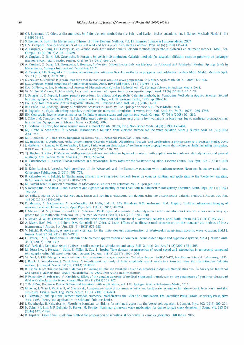
26 P.F. Antonietti et al. / Journal of Computational Physics 415 (2020) 109484

[10] C.E. Baumann, J.T. Oden, A discontinuous hp finite element method for the Euler and Navier—Stokes equations, Int. J. Numer. Methods Fluids 31 (1) (1999) 79–95.

[11] S. Brenner, R. Scott, The Mathematical Theory of Finite Element Methods, vol. 15, Springer Science & Business Media, 2007.[12] D.M. Campbell, Nonlinear dynamics of musical reed and brass wind instruments, Contemp. Phys. 40 (6) (1999) 415–431.[13] A. Cangiani, Z. Dong, E.H. Georgoulis, hp-version space-time discontinuous Galerkin methods for parabolic problems on prismatic meshes, SIAM J. Sci.

Comput. 39 (4) (2017) A1251–A1279.[14] A. Cangiani, Z. Dong, E.H. Georgoulis, P. Houston, hp-version discontinuous Galerkin methods for advection-diffusion-reaction problems on polytopic

meshes, ESAIM: Math. Model. Numer. Anal. 50 (3) (2016) 699–725.[15] A. Cangiani, Z. Dong, E.H. Georgoulis, P. Houston, hp-Version Discontinuous Galerkin Methods on Polygonal and Polyhedral Meshes, SpringerBriefs in

Mathematics, Springer International Publishing, 2017.[16] A. Cangiani, E.H. Georgoulis, P. Houston, hp-version discontinuous Galerkin methods on polygonal and polyhedral meshes, Math. Models Methods Appl.

Sci. 24 (10) (2014) 2009–2041.[17] I. Christov, C. Christov, P. Jordan, Modeling weakly nonlinear acoustic wave propagation, Q. J. Mech. Appl. Math. 60 (4) (2007) 473–495.[18] D.G. Crighton, Model equations of nonlinear acoustics, Annu. Rev. Fluid Mech. 11 (1) (1979) 11–33.[19] D.A. Di Pietro, A. Ern, Mathematical Aspects of Discontinuous Galerkin Methods, vol. 69, Springer Science & Business Media, 2011.[20] W. Dörfler, H. Gerner, R. Schnaubelt, Local well-posedness of a quasilinear wave equation, Appl. Anal. 95 (9) (2016) 2110–2123.[21] J. Douglas Jr., T. Dupont, Interior penalty procedures for elliptic and parabolic Galerkin methods, in: Computing Methods in Applied Sciences, Second

Internat. Sympos., Versailles, 1975, in: Lecture Notes in Phys., vol. 58, Springer, Berlin, 1976, pp. 207–216.[22] F.A. Duck, Nonlinear acoustics in diagnostic ultrasound, Ultrasound Med. Biol. 28 (1) (2002) 1–18.[23] B.O. Enflo, C.M. Hedberg, Theory of Nonlinear Acoustics in Fluids, vol. 67, Springer Science & Business Media, 2006.[24] B. Engquist, A. Majda, Absorbing boundary conditions for numerical simulation of waves, Proc. Natl. Acad. Sci. 74 (5) (1977) 1765–1766.[25] E.H. Georgoulis, Inverse-type estimates on hp-finite element spaces and applications, Math. Comput. 77 (261) (2008) 201–219.[26] J. Gilbert, M. Campbell, A. Myers, B. Pyle, Differences between brass instruments arising from variations in brassiness due to nonlinear propagation, in:

International Symposium on Musical Acoustics (ISMA), 2007.[27] C. Godano, F. Oliveri, Nonlinear seismic waves: a model for site effects, Int. J. Non-Linear Mech. 34 (3) (1999) 457–468.[28] M.J. Grote, A. Schneebeli, D. Schötzau, Discontinuous Galerkin finite element method for the wave equation, SIAM J. Numer. Anal. 44 (6) (2006)

2408–2431.[29] M.F. Hamilton, D.T. Blackstock, Nonlinear Acoustics, Vol. 1, Academic Press, San Diego, 1998.[30] J.S. Hesthaven, T. Warburton, Nodal Discontinuous Galerkin Methods: Algorithms, Analysis, and Applications, Springer Science & Business Media, 2007.[31] J. Hoffelner, H. Landes, M. Kaltenbacher, R. Lerch, Finite element simulation of nonlinear wave propagation in thermoviscous fluids including dissipation,

IEEE Trans. Ultrason. Ferroelectr. Freq. Control 48 (3) (2001) 779–786.[32] T.J. Hughes, T. Kato, J.E. Marsden, Well-posed quasi-linear second-order hyperbolic systems with applications to nonlinear elastodynamics and general

relativity, Arch. Ration. Mech. Anal. 63 (3) (1977) 273–294.[33] B. Kaltenbacher, I. Lasiecka, Global existence and exponential decay rates for the Westervelt equation, Discrete Contin. Dyn. Syst., Ser. S 2 (3) (2009)

503.[34] B. Kaltenbacher, I. Lasiecka, Well-posedness of the Westervelt and the Kuznetsov equation with nonhomogeneous Neumann boundary conditions,

Conference Publications 2 (2011) 763–773.[35] B. Kaltenbacher, V. Nikolic, M. Thalhammer, Efficient time integration methods based on operator splitting and application to the Westervelt equation,

IMA J. Numer. Anal. 35 (3) (2014) 1092–1124.[36] M. Kaltenbacher, Numerical Simulation of Mechatronic Sensors and Actuators, Vol. 2, Springer, 2007.[37] S. Kawashima, Y. Shibata, Global existence and exponential stability of small solutions to nonlinear viscoelasticity, Commun. Math. Phys. 148 (1) (1992)

189–208.[38] J.F. Kelly, S. Marras, X. Zhao, R.J. McGough, Linear and nonlinear ultrasound simulations using the discontinuous Galerkin method, J. Acoust. Soc. Am.

143 (4) (2018) 2438–2448.[39] D. Maresca, A. Lakshmanan, A. Lee-Gosselin, J.M. Melis, Y.-L. Ni, R.W. Bourdeau, D.M. Kochmann, M.G. Shapiro, Nonlinear ultrasound imaging of

nanoscale acoustic biomolecules, Appl. Phys. Lett. 110 (7) (2017) 073704.[40] I. Mazzieri, M. Stupazzini, R. Guidotti, C. Smerzini, SPEED: spectral elements in elastodynamics with discontinuous Galerkin: a non-conforming ap-

proach for 3D multi-scale problems, Int. J. Numer. Methods Fluids 95 (12) (2013) 991–1010.[41] S. Meyer, M. Wilke, Optimal regularity and long-time behavior of solutions for the Westervelt equation, Appl. Math. Optim. 64 (2) (2011) 257–271.[42] A. Myers, R.W. Pyle Jr, J. Gilbert, D.M. Campbell, J.P. Chick, S. Logie, Effects of nonlinear sound propagation on the characteristic timbres of brass

instruments, J. Acoust. Soc. Am. 131 (1) (2012) 678–688.[43] V. Nikolic, B. Wohlmuth, A priori error estimates for the finite element approximation of Westervelt’s quasi-linear acoustic wave equation, SIAM J.

Numer. Anal. 57 (4) (2019) 1897–1918.[44] C. Ortner, E. Süli, Discontinuous Galerkin finite element approximation of nonlinear second-order elliptic and hyperbolic systems, SIAM J. Numer. Anal.

45 (4) (2007) 1370–1397.[45] O.V. Pavlenko, Nonlinear seismic effects in soils: numerical simulation and study, Bull. Seismol. Soc. Am. 91 (2) (2001) 381–396.[46] M. Pérez-Liva, J. Herraiz, J. Udías, E. Miller, B. Cox, B. Treeby, Time domain reconstruction of sound speed and attenuation in ultrasound computed

tomography using full wave inversion, J. Acoust. Soc. Am. 141 (3) (2017) 1595–1604.[47] W. Reed, T. Hill, Triangular mesh methods for the neutron transport equation, Technical Report LA-UR-73-479, Los Alamos Scientific Laboratory, 1973.[48] J. Resch, L. Krivodonova, J. Vanderkooy, A two-dimensional study of finite amplitude sound waves in a trumpet using the discontinuous Galerkin

method, J. Comput. Acoust. 22 (03) (2014) 1450007.[49] B. Rivière, Discontinuous Galerkin Methods for Solving Elliptic and Parabolic Equations, Frontiers in Applied Mathematics, vol. 35, Society for Industrial

and Applied Mathematics (SIAM), Philadelphia, PA, 2008, Theory and implementation.[50] P. Rosnitskiy, P. Yuldashev, V. Khokhlova, Effect of the angular aperture of medical ultrasound transducers on the parameters of nonlinear ultrasound

field with shocks at the focus, Acoust. Phys. 61 (3) (2015) 301–307.[51] T. Roubícek, Nonlinear Partial Differential Equations with Applications, vol. 153, Springer Science & Business Media, 2013.[52] M. Ryles, F. Ngau, I. McDonald, W. Staszewski, Comparative study of nonlinear acoustic and lamb wave techniques for fatigue crack detection in metallic

structures, Fatigue Fract. Eng. Mater. Struct. 31 (8) (2008) 674–683.[53] C. Schwab, p- and hp-Finite Element Methods, Numerical Mathematics and Scientific Computation, The Clarendon Press, Oxford University Press, New

York, 1998, Theory and applications in solid and fluid mechanics.[54] I. Shevchenko, B. Kaltenbacher, Absorbing boundary conditions for nonlinear acoustics: the Westervelt equation, J. Comput. Phys. 302 (2015) 200–221.[55] H. Sohn, H.J. Lim, M.P. DeSimio, K. Brown, M. Derriso, Nonlinear ultrasonic wave modulation for online fatigue crack detection, J. Sound Vib. 333 (5)

(2014) 1473–1484.[56] B. Tripathi, Discontinuous Galerkin method for propagation of acoustical shock waves in complex geometry, PhD thesis, 2015.

P.F. Antonietti et al. / Journal of Computational Physics 415 (2020) 109484 27

[57] B.B. Tripathi, A. Luca, S. Baskar, F. Coulouvrat, R. Marchiano, Element centered smooth artificial viscosity in discontinuous Galerkin method for propa-gation of acoustic shock waves on unstructured meshes, J. Comput. Phys. 366 (2018) 298–319.

[58] T. Tsuchiya, Y. Kagawa, A simulation study on nonlinear sound propagation by finite element approach, J. Accoust. Soc. Jpn. 13 (4) (1992) 223–230.[59] P.J. Westervelt, Parametric acoustic array, J. Acoust. Soc. Am. 35 (4) (1963) 535–537.