Monitoring fish using passive acoustics by Xavier Mouy B.Sc ...

Monitoring fish using passive acoustics

by

Xavier Mouy

B.Sc., University of Le Mans, 2004

M.Sc., University of Quebec in Rimouski, 2007

A Dissertation Submitted in Partial Fulfillment of the

Requirements for the Degree of

DOCTOR OF PHILOSOPHY

in the School of Earth and Ocean Sciences

© Xavier Mouy, 2022

University of Victoria

All rights reserved. This dissertation may not be reproduced in whole or in part, by

photocopying or other means, without the permission of the author.

ii

Monitoring fish using passive acoustics

by

Xavier Mouy

B.Sc., University of Le Mans, 2004

M.Sc., University of Quebec in Rimouski, 2007

Supervisory Committee

Dr. S. E. Dosso, Co-Supervisor

(School of Earth and Ocean Sciences)

Dr. F. Juanes, Co-Supervisor

(Department of Biology)

Dr. J. F. Dower, Departmental Member

(School of Earth and Ocean Sciences)

Dr. G. Tzanetakis, Outside Member

(Department of Computer Science)

Dr. R. A. Rountree, Outside Member

(Department of Biology)

iii

ABSTRACT

Some fish produce sounds for a variety of reasons, such as to find mates, defend

their territory, or maintain cohesion within their group. These sounds could be used

to non-intrusively detect the presence of fish and potentially to estimate their number

(or density) over large areas and long time periods. However, many fish sounds have

not yet been associated to specific species, which limits the usefulness of this approach.

While recording fish sounds in tanks is reasonably straightforward, it presents several

problems: many fish do not produce sounds in captivity or their behavior and sound

production is altered significantly, and the complex acoustic propagation conditions

in tanks often leads to distorted measurements. The work presented in this thesis

aims to address these issues by providing methodologies to record, detect, and iden-

tify species-specific fish sounds in the wild. A set of hardware and software solutions

are developed to simultaneously record fish sounds, acoustically localize the fish in

three-dimensions, and record video to identify the fish and observe their behavior.

Three platforms have been developed and tested in the field. The first platform, re-

ferred to as the large array, is composed of six hydrophones connected to an AMAR

acoustic recorder and two open-source autonomous video cameras (FishCams) that

were developed during this thesis. These instruments are secured to a PVC frame

of dimension 2 m x 2 m x 3 m that can be transported and assembled in the field.

The hydrophone configuration for this array was defined using a simulated annealing

optimization approach that minimized localization uncertainties. This array provides

the largest field of view and most accurate acoustic localization, and is well suited

to long-term deployments (weeks). The second platform, referred to as the mini ar-

ray, uses a single FishCam and four hydrophones connected to a SoundTrap acoustic

recorder on a one cubic meter PVC frame; this array can be deployed more easily in

constrained locations or on rough/uneven seabeds. The third platform, referred to as

the mobile array, consists of four hydrophones connected to a SoundTrap recorder and

mounted on a tethered Trident underwater drone with built-in video, allowing remote

control and real-time positioning in response to observed fish presence, rather than

long-term deployments as for the large and mini arrays. For each array, acoustic lo-

calization is performed by measuring time-difference of arrivals between hydrophones

and estimating the sound-source location using linearized (for the large array) or

non-linear (for the mini and mobile arrays) inversion. Fish sounds are automatically

detected and localized in three dimensions, and sounds localized within the field of

iv

view of the camera(s) are assigned to a fish species by manually reviewing the video

recordings. The three platforms were deployed at four locations off the East coast of

Vancouver Island, British Columbia, Canada, and allowed the identification of sounds

from quillback rockfish (Sebastes maliger), copper rockfish (Sebastes caurinus), and

lingcod (Ophiodon elongatus), species that had not been documented previously to

produce sounds. While each platform developed during this thesis has its own set

of advantages and limitations, using them in coordination helps identify fish sounds

over different habitats and with various budget and logistical constraints. In an effort

to make passive acoustics a more viable way to monitor fish in the wild, this thesis

also investigates the use of automatic detection and classification algorithms to ef-

ficiently find fish sounds in large passive acoustic datasets. The proposed approach

detects acoustic transients using a measure of spectrogram variance and classifies

them as “noise” or “fish sounds” using a binary classifier. Five different classification

algorithms were trained and evaluated on a dataset of more than 96,000 manually-

annotated examples of fish sounds and noise from five locations off Vancouver Island.

The classification algorithm that performed best (random forest) has an Fscore of

0.84 (Precision = 0.82, Recall = 0.86) on the test dataset. The analysis of 2.5

months of acoustic data collected in a rockfish conservation area off Vancouver Island

shows that the proposed detector can be used to efficiently explore large datasets,

formulate hypotheses, and help answer practical conservation questions.

v

Contents

Supervisory Committee ii

Abstract iii

Table of Contents v

List of Tables ix

List of Figures x

Acknowledgements xx

Dedication xxii

1 Introduction 1

1.1 Background and motivation . . . . . . . . . . . . . . . . . . . . . . . 1

1.2 Thesis outline . . . . . . . . . . . . . . . . . . . . . . . . . . . . . . . 6

2 Cataloging fish sounds in the wild using acoustic localization and

video recordings: a proof of concept 7

2.1 Abstract . . . . . . . . . . . . . . . . . . . . . . . . . . . . . . . . . . 7

2.2 Introduction . . . . . . . . . . . . . . . . . . . . . . . . . . . . . . . . 8

2.3 Methods . . . . . . . . . . . . . . . . . . . . . . . . . . . . . . . . . . 9

2.3.1 Array and data collection . . . . . . . . . . . . . . . . . . . . 9

2.3.2 Automated detection of acoustic events . . . . . . . . . . . . . 10

2.3.3 Acoustic localization by linearized inversion . . . . . . . . . . 10

2.3.4 Video processing . . . . . . . . . . . . . . . . . . . . . . . . . 12

2.4 Results . . . . . . . . . . . . . . . . . . . . . . . . . . . . . . . . . . . 13

2.5 Discussion . . . . . . . . . . . . . . . . . . . . . . . . . . . . . . . . . 15

2.6 Acknowledgements . . . . . . . . . . . . . . . . . . . . . . . . . . . . 15

vi

3 Development of a low-cost open source autonomous camera for

aquatic research 17

3.1 Abstract . . . . . . . . . . . . . . . . . . . . . . . . . . . . . . . . . . 17

3.2 Hardware in context . . . . . . . . . . . . . . . . . . . . . . . . . . . 18

3.3 Hardware description . . . . . . . . . . . . . . . . . . . . . . . . . . . 19

3.3.1 Electronic design . . . . . . . . . . . . . . . . . . . . . . . . . 19

3.3.2 Mechanical design . . . . . . . . . . . . . . . . . . . . . . . . . 20

3.3.3 Software . . . . . . . . . . . . . . . . . . . . . . . . . . . . . . 23

3.4 Validation and characterization . . . . . . . . . . . . . . . . . . . . . 26

3.5 Summary . . . . . . . . . . . . . . . . . . . . . . . . . . . . . . . . . 32


4 Identifying fish sounds in the wild: development and comparison

of three audio/video platforms 34

4.1 Abstract . . . . . . . . . . . . . . . . . . . . . . . . . . . . . . . . . . 34

4.2 Introduction . . . . . . . . . . . . . . . . . . . . . . . . . . . . . . . . 35

4.3 Methods . . . . . . . . . . . . . . . . . . . . . . . . . . . . . . . . . . 38

4.3.1 Description of the audio/video arrays . . . . . . . . . . . . . . 38

4.3.2 Automatic detection of acoustic transients . . . . . . . . . . . 42

4.3.3 Time Difference of Arrival . . . . . . . . . . . . . . . . . . . . 44

4.3.4 Acoustic localization . . . . . . . . . . . . . . . . . . . . . . . 44

4.3.5 Identification of the localized sounds . . . . . . . . . . . . . . 47

4.3.6 Optimization of hydrophone placement . . . . . . . . . . . . . 47

4.3.7 Characterization of identified fish sounds . . . . . . . . . . . . 49

4.3.8 Estimation of source levels . . . . . . . . . . . . . . . . . . . . 51

4.3.9 Software implementation . . . . . . . . . . . . . . . . . . . . . 52

4.3.10 Data collection in the field . . . . . . . . . . . . . . . . . . . . 52

4.3.11 Localization of controlled sound sources in the field . . . . . . 55

4.4 Results . . . . . . . . . . . . . . . . . . . . . . . . . . . . . . . . . . . 56

4.4.1 Identification of fish sounds using the large array . . . . . . . 56

4.4.2 Identification of fish sounds using the mini array . . . . . . . . 60

4.4.3 Identification of fish sounds using the mobile array . . . . . . 63

4.4.4 Description of identified fish sounds . . . . . . . . . . . . . . . 63

4.5 Discussion . . . . . . . . . . . . . . . . . . . . . . . . . . . . . . . . . 68

4.6 Summary . . . . . . . . . . . . . . . . . . . . . . . . . . . . . . . . . 72

vii

4.7 Acknowledgments . . . . . . . . . . . . . . . . . . . . . . . . . . . . . 73

5 Automatic detection and classification of fish sounds in British

Columbia 75

5.1 Abstract . . . . . . . . . . . . . . . . . . . . . . . . . . . . . . . . . . 75

5.2 Introduction . . . . . . . . . . . . . . . . . . . . . . . . . . . . . . . . 76

5.3 Methods . . . . . . . . . . . . . . . . . . . . . . . . . . . . . . . . . . 78

5.3.1 Data Set . . . . . . . . . . . . . . . . . . . . . . . . . . . . . . 78

5.3.2 Detection . . . . . . . . . . . . . . . . . . . . . . . . . . . . . 82

5.3.3 Feature extraction . . . . . . . . . . . . . . . . . . . . . . . . 84

5.3.4 Classification . . . . . . . . . . . . . . . . . . . . . . . . . . . 87

5.3.5 Experimental Design . . . . . . . . . . . . . . . . . . . . . . . 90

5.3.6 Performance . . . . . . . . . . . . . . . . . . . . . . . . . . . . 92

5.3.7 Implementation . . . . . . . . . . . . . . . . . . . . . . . . . . 93

5.4 Results . . . . . . . . . . . . . . . . . . . . . . . . . . . . . . . . . . . 94

5.5 Discussion and conclusion . . . . . . . . . . . . . . . . . . . . . . . . 96


6 Discussion and Perspectives 100

A FishCam User Manual: Instructions to build, configure and oper-

ate the FishCam 107

A.1 Bill of materials . . . . . . . . . . . . . . . . . . . . . . . . . . . . . . 108

A.2 Build instructions . . . . . . . . . . . . . . . . . . . . . . . . . . . . . 109

A.2.1 Assembling the electronics . . . . . . . . . . . . . . . . . . . . 109

A.2.2 Building the internal frame . . . . . . . . . . . . . . . . . . . 119

A.2.3 Building the pressure housing and external attachment . . . . 130

A.2.4 Installing the D-cell batteries . . . . . . . . . . . . . . . . . . 132

A.3 Operation instructions . . . . . . . . . . . . . . . . . . . . . . . . . . 135

A.3.1 Installing the software suite . . . . . . . . . . . . . . . . . . . 135

A.3.2 Automatic start of the recordings . . . . . . . . . . . . . . . . 138

A.3.3 FishCam ID . . . . . . . . . . . . . . . . . . . . . . . . . . . . 138

A.3.4 Camera settings . . . . . . . . . . . . . . . . . . . . . . . . . . 139

A.3.5 Configuring the duty cycles . . . . . . . . . . . . . . . . . . . 139

A.3.6 Configuring the buzzer . . . . . . . . . . . . . . . . . . . . . . 140

A.3.7 Accessing the FishCam wirelessly . . . . . . . . . . . . . . . . 141

viii

A.3.8 Downloading data from the FishCam . . . . . . . . . . . . . . 146

A.3.9 Pre-deployment checklist . . . . . . . . . . . . . . . . . . . . . 146

Bibliography 148

ix

List of Tables

3.1 Deployments of the FishCam in the field. . . . . . . . . . . . . . . . 28

4.1 Deployment locations, depths, and durations. . . . . . . . . . . . . . 53

4.2 Characteristics of the fish sounds identified. Duration, pulse frequency,

pulse rate, and source level are reported by their mean ± the standard

deviation. Asterisks (∗) indicate measurements for which there were

not enough samples of fish sounds (n) to estimate the standard deviation. 68

5.1 Fish and noise annotations used to develop the fish sound classifier. . 79

5.2 Description of the features calculated for each detection. . . . . . . . 86

5.3 Performance of all the classification models on the training data set

for a confidence threshold of 0.5 (mean ± standard deviation). RF5,

RF10, RF30, and RF50 correspond to the RF models trained with 5,

10, 30, and 50 trees, respectively. . . . . . . . . . . . . . . . . . . . . 95

5.4 Performance of the random forest model with 50 trees on the test data

set for a confidence threshold of 0.5. This model was trained using the

entire training data set. . . . . . . . . . . . . . . . . . . . . . . . . . 96

6.1 Estimated detection range (R) of fish sounds at Mill Bay and Horbny

Island. Noise levels (NL) were computed in the 20-1000 Hz frequency

band every minute by averaging 120 1 s long Hann-windowed fast

Fourier transforms overlapped by 0.5 s. . . . . . . . . . . . . . . . . . 105

A.1 Bill of material . . . . . . . . . . . . . . . . . . . . . . . . . . . . . . 108

x

List of Figures

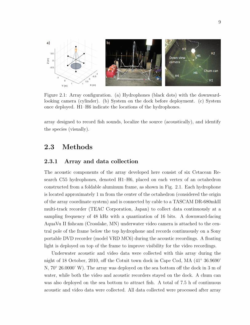
2.1 Array configuration. (a) Hydrophones (black dots) with the downward-

looking camera (cylinder). (b) System on the dock before deployment.

(c) System once deployed. H1–H6 indicate the locations of the hy-

drophones. . . . . . . . . . . . . . . . . . . . . . . . . . . . . . . . . 9

2.2 Localization uncertainties of the hydrophone array in the (a) XY, (b)

XZ, and (c) YZ plane. . . . . . . . . . . . . . . . . . . . . . . . . . . 13

2.3 Identification of sounds produced by a tautog. (a) Image from the

video camera showing the tautog swimming in the middle of the array

(red pixels). (b) Simultaneous acoustic localization (red dots) with

uncertainties on each axis (blue lines). (c) Spectrogram of the sounds

recorded on hydrophone 2. Red boxes indicate the sounds automati-

cally detected by the detector that were used for the localization. . . 14

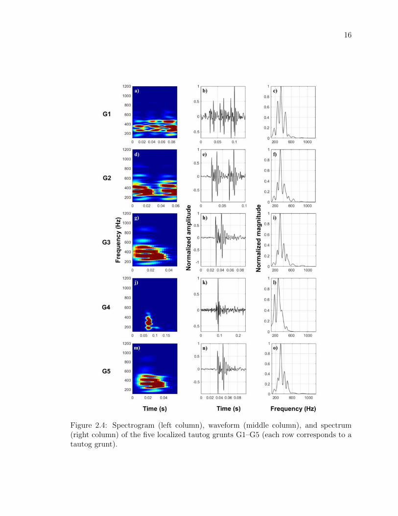
2.4 Spectrogram (left column), waveform (middle column), and spectrum

(right column) of the five localized tautog grunts G1–G5 (each row

corresponds to a tautog grunt). . . . . . . . . . . . . . . . . . . . . . 16

3.1 Overview of the FishCam . . . . . . . . . . . . . . . . . . . . . . . . 21

3.2 Internal frame . . . . . . . . . . . . . . . . . . . . . . . . . . . . . . 22

3.3 External components . . . . . . . . . . . . . . . . . . . . . . . . . . . 24

3.4 Video examples . . . . . . . . . . . . . . . . . . . . . . . . . . . . . . 29

3.5 Synchronization tones . . . . . . . . . . . . . . . . . . . . . . . . . . 30

4.1 Large array. (a) Photograph of the large array deployed in the field.

(b) side view and (c) top view diagrams of the array with dimensions.

The six hydrophones are represented by the numbered gray circles.

The top and side video cameras are indicated by C1 and C2, respec-

tively. Note that C1 is not represented in (c) for clarity. The acoustic

recorder and its battery pack are indicated by AR and PB, respec-

tively. Gray and red lines represent the PVC structure of the array

(red indicating the square base of the array). . . . . . . . . . . . . . 39

xi

4.2 Mini audio and video array. (a) Photograph of the mini array before

deployment in the field. (b) rear view and (c) top view diagrams of the

mini array with dimensions. The four hydrophones are represented by

the numbered gray circles. The camera and the acoustic recorder are

indicated by C and AR, respectively. Grey and black lines represent

the frame of the array. . . . . . . . . . . . . . . . . . . . . . . . . . . 41

4.3 Mobile audio and video array. (a) Photograph of the mobile array

deployed in the field. (b) rear view and (c) top view diagrams of the

mobile array with dimensions. The four hydrophones are represented

by the numbered gray circles. The underwater drone and the acoustic

recorder are indicated by ROV and AR, respectively. The video cam-

era is located at the front of the drone (coordinates: (0,0.2,−0.05))

facing forward. Black lines represent the frame of the array. . . . . . 42

4.4 Optimization of hydrophone placement using simulated annealing: X

(top row), Y (middle row), and Z (bottom row) coordinates of each

hydrophone (columns) at each iteration of the simulated annealing

process. . . . . . . . . . . . . . . . . . . . . . . . . . . . . . . . . . . 49

4.5 Comparison of localization uncertainties between the large array from

this study and the array used in [76]. (a) Hydrophone geometry used

in [76]. (b) Hydrophone geometry of the large array as defined by the

simulated annealing optimization process. Estimated 50-cm localiza-

tion uncertainty isoline of the large array (dashed line) and [76] (solid

line) in the (c) XY , (d) XZ, and (e) Y Z plane. Uncertainties for each

array were computed using Eq. 4.10 on a 3D grid of 3 m3 with points

located every 10 cm, and using a standard deviation of data errors of

0.12 ms. . . . . . . . . . . . . . . . . . . . . . . . . . . . . . . . . . . 50

4.6 Waveform of a fish grunt composed of six pulses. The pulse period,

Tpulse, and pulse repetition interval, Trep, are measured on the wave-

form representation of the fish sound to calculate the pulse frequency

and pulse repetition rate, respectively. Tdur represents the duration of

the sound. . . . . . . . . . . . . . . . . . . . . . . . . . . . . . . . . . 51

4.7 Map of the deployment locations. Black dots indicate the locations

where the audio and video arrays were deployed. . . . . . . . . . . . 54

xii

4.8 Acoustic localization of the underwater drone using the large array

deployed at Ogden Point (17 Jun. 2019). (a) Spectrogram of the

acoustic recording acquired by hydrophone 4 (frame: 0.0624 s, FFT:

0.0853 s, step size: 0.01 s, Hanning window). Beige boxes indicate

the time and frequency limits of the sounds that were automatically

detected. Dots at the top of the spectrogram indicate the colors as-

sociated to the start time of each detection (see color scale on the

x-axis) and used for the localization. Colored camera icons indicate

the time of the camera frames shown in panels (d) and (e). (b) Side

and (c) top view of the large array. Colored dots and lines represent

the coordinates and uncertainty (standard deviation) of the acoustic

localizations, respectively. (d) Image taken by video camera C2 at

t = 1.2 s, and (e) t = 5 s, showing the underwater drone approaching

the array. Numbers in panels (b), (c), (d), and (e) correspond to the

hydrophone identification numbers. . . . . . . . . . . . . . . . . . . . 57

4.9 Acoustic localization of the underwater drone using the mini array de-

ployed at Mill Bay (1 Aug. 2019). (a) Spectrogram of the acoustic

recording acquired by hydrophone 2 (frame: 0.0624 s, FFT: 0.0853 s,

step size: 0.01 s, Hanning window). Beige boxes indicate the time and

frequency limits of the underwater drone sounds that were automati-

cally detected. Dots at the top of the spectrogram indicate the colors

associated to the start time of each detection (see color scale on the

x-axis) and used for the localization. The green camera icon indicates

the time of the camera frames showed in panels (d) and (e). (b) Rear

and (c) top view of the mini array. Colored dots and lines represent

the coordinates and uncertainty (99% highest-probability density cred-

ibility interval) of the acoustic localizations, respectively. (d) Image

taken by the underwater drone at t = 4.7 s showing the mini array.

(e) Image taken from the video camera of the mini array at t = 4.7 s,

showing the underwater drone in front of the array. . . . . . . . . . . 58

xiii

4.10 Localization of an acoustic projector using the mobile array deployed

at Macaulay Point (10 Sep. 2020). (a) Spectrogram of the acoustic



frequency limits of the fish sounds that were emitted by the acoustic

projector and automatically detected. (b) Rear and (c) top view of

the mobile array. Colored dots and lines represent the coordinates

and uncertainty (99% highest-probability density credibility interval)

of the acoustic localizations, respectively. Red, green, orange, and

blue correspond to acoustic localizations when the acoustic projector

was located at coordinates (0,1,0), (1,0,0), (0,−1,0), and (−1,0,0),

respectively. . . . . . . . . . . . . . . . . . . . . . . . . . . . . . . . . 59

4.11 Identification of sounds from lingcod using the large array deployed at

Ogden Point (17 Jun. 2019). (a) Spectrogram of the acoustic record-

ing acquired by hydrophone 4 (frame: 0.0624 s, FFT: 0.0853 s, step

size: 0.01 s, Hanning window). Beige boxes indicate the time and

frequency limits of the fish sounds that were automatically detected.

Dots at the top of the spectrogram indicate the colors associated to the

start time of each detection (see color scale on the x-axis) and used

for the localization. Colored camera icons indicate the time of the

camera frames shown in panels (d) and (e). (b) Side and (c) top view

of the large array. Colored dots and lines represent the coordinates

and uncertainty (standard deviation) of the acoustic localizations, re-

spectively. (d) Image taken by video camera C1 at t = 0.5 s, and (e)

t = 6 s, showing a lingcod entering the array from the left and stopping

at the center of the array on the seafloor below hydrophone 4. Bold

numbers in panels (b), (c), (d), and (e) correspond to the hydrophone

identification numbers. Video available on the data repository [133]. . 61

xiv

4.12 Identification of sounds from quillback rockfish using the large array

deployed at Hornby Island (20 Sep. 2019). (a) Spectrogram of the



the time and frequency limits of the fish sounds that were automati-



x-axis) and used for the localization. Colored camera icons indicate

the time of the camera frames showed in panels (d) and (e). (b) Side

and (c) top view of the large array. Colored dots and lines represent

the coordinates and uncertainty (standard deviation) of the acoustic

localizations, respectively. (d) Image taken by video camera C1 at

t = 2 s, and (e) t = 10 s, showing a lingcod and three quillback rock-

fish near or inside the array. Bold numbers in panels (b), (c), (d),

and (e) correspond to the hydrophone identification numbers. Video

available on the data repository [133]. . . . . . . . . . . . . . . . . . 62

4.13 Identification of sounds from copper rockfish using the mini array de-

ployed at Mill Bay (1 Aug. 2019). (a) Spectrogram of the acoustic




Dots at the top of the spectrogram indicate the colors associated to

the start time of each detection (see color scale on the x-axis) and used

for the localization. The blue camera icon indicates the time of the

camera frame showed in panel (e). (b) Rear and (c) top view of the

mini array. Colored dots and lines represent the coordinates and un-

certainty (99% highest-probability density credibility interval) of the

acoustic localizations, respectively. (d) Image from the video camera,

taken several minutes before the fish sounds were emitted, showing the

copper rockfish before it sat on top of the mini array. (e) Image taken

from the video camera of the mini array at t = 0.5 s, showing the tail

of the copper rockfish sitting on top of the mini array. Video available

on the data repository [133]. . . . . . . . . . . . . . . . . . . . . . . . 64

xv

4.14 Identification of sounds from copper rockfish using the mobile array

deployed at Hornby Island (21 Sep. 2019). (a) Spectrogram of the



the time and frequency limits of the fish sounds that were automati-



x-axis) and used for the localization. The yellow camera icon indicates

the time of the camera frame showed in panel (d). (b) Rear and (c)

top view of the mobile array. Colored dots and lines represent the co-

ordinates and uncertainty (99% highest-probability density credibility

interval) of the acoustic localizations, respectively. (d) Image from the

underwater drone’s video camera and taken at t = 11.9 s, showing two

copper rockfish at the front of the mobile array. Video available on

the data repository [133]. . . . . . . . . . . . . . . . . . . . . . . . . 65

4.15 Localization of unknown fish sounds using the mobile array deployed

at Hornby Island (18 Sep. 2019). (a) Spectrogram of the acoustic






for the localization. The green camera icon indicates the time of the

camera frame showed in panel (d). (b) Rear and (c) top view of the

mobile array. Colored dots and lines represent the coordinates and

uncertainty (99% highest-probability density credibility interval) of

the acoustic localizations, respectively. (d) Image from the underwater

drone’s video camera taken at t = 5.9 s, showing a blackeye goby and

a copper rockfish in front of the mobile array. Video available on the

data repository [133]. . . . . . . . . . . . . . . . . . . . . . . . . . . . 66

xvi

4.16 Localization of unknown fish sounds using the mobile array deployed

at Hornby Island (16 Sep. 2019). (a) Spectrogram of the acoustic






for the localization. The turquoise camera icon indicates the time of

the camera frame shown in (d). (b) Rear and (c) top view of the

mobile array. Colored dots and lines represent the coordinates and

uncertainty (99% highest-probability density credibility interval) of

the acoustic localizations, respectively. (d) Image from the underwater

drone’s video camera taken at t = 3.8 s, showing a blackeye goby in

front of the mobile array, defending its territory. Video available on

the data repository [133]. . . . . . . . . . . . . . . . . . . . . . . . . 67

4.17 Illustration of the different constraints, strengths, and weaknesses of

each audio/video array proposed in this study . . . . . . . . . . . . . 71

5.1 Spectrogram of unknown fish knock and grunt sounds recorded off

Hornby Island, British Columbia (1.95 Hz frequency resolution, 0.128

s time window, 0.012 s time step, Hamming window). Knocks are the

short pulses and grunts the longer sounds with an harmonic structure. 77

5.2 Example of fish (a) and (b) noise sounds manually annotated with

PAMlab. The yellow boxes indicate the time and frequency boundaries

of the sound defined by the analyst (a) or the detector (b) on the

spectrogram (1.95 Hz frequency resolution, 0.128 s time window, 0.012

s time step, Hamming window). “FS” and “NN” indicate annotated

fish and noise sounds, respectively. . . . . . . . . . . . . . . . . . . . 80

5.3 Map of the sampling locations. Black dots indicate the location of the

acoustic recorders that were used to create the manually annotated fish

and noise sound data sets. NC-RCA In and NC-RCA Out indicate

recorders deployed inside and outside the Northumberland Channel

Rockfish Conservation Area, respectively. . . . . . . . . . . . . . . . 81

xvii

5.4 Illustration of the detection process on a recording containing three

fish sounds. a) Equalized spectrogram S[t, f ], b) local variance matrix

Svar[t, f ], c) binarized spectrogram, d) result of the detection process.

Red boxes indicate the time and frequency boundaries of each detected

event. Fish sounds are at t = 0.2 s, t = 1.5 s, and t = 2.8 s. . . . . . 83

5.5 Extraction of features. a) Spectrogram of a fish detection. Red and

black crosses denote the median and peak frequency of each time slice

of the spectrogram, respectively. The white box indicates the 95%

energy area over which the spectrogram features were calculated. b)

Spectral envelope of the detection. c) Temporal envelope of the detec-

tion. . . . . . . . . . . . . . . . . . . . . . . . . . . . . . . . . . . . . 85

5.6 Description of the data used in the training and testing data sets.

Labels on the x-axis indicate the class of the annotations (i.e., fish or

noise) followed by the identification of the deployment they were from

(see Table 5.1). . . . . . . . . . . . . . . . . . . . . . . . . . . . . . . 90

5.7 Illustration of the protocol used to train and evaluate the performance

of the different classification models. . . . . . . . . . . . . . . . . . . 91

5.8 Performance of the fish sound classifier on the training data set: a)

Average precision and recall and (b) average F score calculated over

all confidence thresholds for the eight (plus the dummy baseline) clas-

sification models tested. . . . . . . . . . . . . . . . . . . . . . . . . . 94

5.9 Automatic detection of fish sounds inside the Northumberland Chan-

nel RCA from April to June 2019. a) Spectrogram of a 30 s recording

from May 19 with no fish sounds, b) heat map representation of the

number of automatic fish detections per hour, c) spectrogram of a 30

s recording from May 26 with more than 60 fish sounds. Spectrogram

resolution: 1.95 Hz frequency resolution, 0.128 s time window, 0.012 s

time step, Hamming window. . . . . . . . . . . . . . . . . . . . . . . 98

6.1 Conceptual diagram of the different modules in ecosound. Blue rect-

angles denote the ecosound base objects, and blue dashed arrows refer

to visual representations. . . . . . . . . . . . . . . . . . . . . . . . . . 102

6.2 Pulse frequency and duration of the single pulse sounds idendified in

Chapter 4. . . . . . . . . . . . . . . . . . . . . . . . . . . . . . . . . . 103

A.1 Raspberry Pi zero with male header . . . . . . . . . . . . . . . . . . 109

A.2 Soldering of the JST male connector on the Witty Pi. . . . . . . . . . 109

xviii

A.3 Installation of the silicon mounts. . . . . . . . . . . . . . . . . . . . . 110

A.4 Installation of Witty Pi. . . . . . . . . . . . . . . . . . . . . . . . . . 111

A.5 Preparation of the voltage regulator. . . . . . . . . . . . . . . . . . . 112

A.6 Installation of the JST female connector. . . . . . . . . . . . . . . . . 112

A.7 Assembly of Molex Connector, ON/OFF switch, voltage regulator,

and Raspberry Pi. . . . . . . . . . . . . . . . . . . . . . . . . . . . . 113

A.8 Installation of the camera sensor on its mount. . . . . . . . . . . . . 114

A.9 Electronic diagram of the buzzer circuit. . . . . . . . . . . . . . . . . 114

A.10 Buzzer circuit. . . . . . . . . . . . . . . . . . . . . . . . . . . . . . . 115

A.11 Assembly of all the electronic components. . . . . . . . . . . . . . . . 117

A.12 Placement of the electronic components on the mounting plate. . . . 118

A.13 Electronic components installed on the mounting plate. . . . . . . . . 120

A.14 Cutting of the discs from the PVC vinyl tile. . . . . . . . . . . . . . 120

A.15 Sanding edges of the discs. . . . . . . . . . . . . . . . . . . . . . . . . 121

A.16 Locating holes to drill on the discs. . . . . . . . . . . . . . . . . . . . 121

A.17 Drilling of the holes on the discs. . . . . . . . . . . . . . . . . . . . . 122

A.18 Battery connectors glued to the discs. . . . . . . . . . . . . . . . . . 123

A.19 Cutting of the metal rods. . . . . . . . . . . . . . . . . . . . . . . . . 124

A.20 Assembly of the rods and discs. . . . . . . . . . . . . . . . . . . . . . 125

A.21 Assembly of the negative discs. . . . . . . . . . . . . . . . . . . . . . 126

A.22 Soldering of the Molex connector. . . . . . . . . . . . . . . . . . . . . 126

A.23 Attachment of the handle. . . . . . . . . . . . . . . . . . . . . . . . . 127

A.24 Assembly of the electronics with the internal frame. . . . . . . . . . . 128

A.25 Connection of the electronics to the battery pack. . . . . . . . . . . . 128

A.26 Assembly of the cap nut and screw protector. . . . . . . . . . . . . . 129

A.27 Inside of the Fishcam fully assembled. . . . . . . . . . . . . . . . . . 129

A.28 Cutting of the tee fitting. . . . . . . . . . . . . . . . . . . . . . . . . 130

A.29 Installation of the bushing on the tee fitting. . . . . . . . . . . . . . . 131

A.30 Installation of the PVC union fittings. . . . . . . . . . . . . . . . . . 131

A.31 Installation of PVC attachments to the pressure housing of the Fishcam.132

A.32 Installation of the D-cell batteries in the central stack. . . . . . . . . 133

A.33 Installation of the rest of the D-cell batteries. . . . . . . . . . . . . . 134

A.34 Illustration of the parameters defining the beeping sequences of the

buzzer. . . . . . . . . . . . . . . . . . . . . . . . . . . . . . . . . . . 141

A.35 Setting up a Wi-fi hotspot. . . . . . . . . . . . . . . . . . . . . . . . 142

xix

A.36 FishCam connected to the wi-fi hotspot. . . . . . . . . . . . . . . . . 144

A.37 RaspController’s interface to control and monitor the FishCam. . . . 144

A.38 Monitoring the status of the data acquisition. . . . . . . . . . . . . . 145

xx

ACKNOWLEDGEMENTS

I would like to thank:

My supervisors Dr. Stan Dosso and Dr. Francis Juanes. I could not have

hoped for better supervisors. Francis helped me learn more about fish biology

and ecology, and Stan substantially deepened my knowledge of acoustics and

inversion methods. They both were always available when I needed, despite

their numerous commitments and responsibilities. I am tremendously grateful

to have had the opportunity to work with them. Beside the academic aspect,

Stan and Francis are just wonderful people who have always been kind and

supportive to me, my wife, and my kids. Chatting with them on a regular

basis, particularly during the pandemic, was always uplifting and really helped

me get through the hard times.

Dr. Rodney Rountree who has been such a great inspiration and mentor for this

work. Most of the research conducted in this thesis is the realization of visionary

ideas Rodney already had several decades ago. I thank him for sharing his

experience, stories, and “big picture” ideas that helped me put my work into

perspective.

Morgan Black, Kieran Cox, and Jessica Qualley for leading all the diving

operations and being such great friends and colleagues.

All the volunteers who helped me during fieldwork, including: Tristan Blaine

(CCIRA), Nick Bohlender (UVic), Jenna Bright (Archipelago), Desiree Bulger

(UVic), Garth Covernton (UVic), Hailey Davies (UVic), Sean Dimoff (UVic),

Sarah Dudas (DFO), Heloise Frouin-Mouy (UVic), Dana Haggarty (DFO),

Katie Innes (UVic), Alex MacGillivray (JASCO), Jesse Macleod (UVic), Niallan

O’Brien (UVic), Kristina Tietjen (UVic), Brian Timmer (UVic), Scott Trivers

(Indep.),

David Hannay and Dr. Roberto Racca for their mentorship and for allowing

me to keep working at JASCO Applied Sciences part-time during my PhD.

My wife and kids. Heloıse was supportive of my decision to go back to school

right from the beginning. She helped with many aspects of my PhD, cheered

me up in difficult times and was also there when it was time to celebrate. I

xxi

am also so grateful that she tolerated to have electronic components all over

our house and a big PVC frame in our backyard for several months. Hugo and

Charlotte always made me feel good about my work and were always keen to

help when they could, and learn about what I had been building or discovering.

Most importantly, they helped me keep my feet on the ground and constantly

reminded me that there is nothing more important than family.

My parents to have pushed me to continue my studies 20 years ago, when all I

wanted was to play music with my friends. Who would have thought I would

end up with a PhD...(certainly not me). The work I do is my passion and it is

in large part thanks to them. I can’t thank them enough for this. Thanks also

to my sister Elizabeth, and my two brothers, Pierre-Alain and Yann, for their

encouragements, the lovely packages full of French treats they sent me, and for

always being there when I needed to talk.

All my friends in Canada and France who supported me in many different ways.

Thanks Chris and Claire, Alexis and Herman, Adrien, Amalis, Ben and Celia,

Alex and Natalie, Graham and Shyla for these unforgettable moments spent

in Victoria with you. Thanks Rianna and Dave for these much needed coffee

breaks in the Whale Lab at UVic, the fun times with the kids and the won-

derful memories on Flores Island. Thanks Amalis for these precious discussions

at SEOS and for listening to me rambling about my equipment and various

struggles. Thanks to Mitch and Caro, Julien Pommier, Florian, and Cedric for

your always-encouraging phone calls and emails.

”You got it, Cap!”

Tweak from the Octonauts

xxii

DEDICATION

To my parents Marie-Christine and Alain Mouy

Chapter 1

Introduction

1.1 Background and motivation

The first written recognition that fish produce sound was made by Aristotle in the 4th

century BC, who observed that “Fishes can produce no voice, for they have no lungs,

nor windpipe and pharynx; but they emit certain inarticulate sounds and squeaks.”

[1]. In the middle of the 19th century, several scientific studies confirmed Aristotle’s

observation by describing the sound-producing mechanisms of several species of fish

[2, 3]. In the 1950s to early 1970s, key scientific studies listed and described the sounds

of a large variety of fish species from both the Pacific and Western North Atlantic

Ocean [4–6]. Anecdotally, in 1968, Captain Jacques Yves Cousteau also exposed the

general public to fish sounds in the episode “Savage World of the Coral Jungle” of

the popular television documentaries “The Undersea World of Jacques Cousteau”

[7]. Even though fish have been known to produce sounds for a very long time,

their acoustic repertoire and acoustic behaviour have arguably been under-studied

compared to acoustic research on marine mammals.

Over 800 species of fishes worldwide are known to be soniferous [8, 9]. More than

150 of these species are found in the northwest Atlantic [6]. Among the approximately

400 known marine fish species frequenting the waters of British Columbia, only 22

have been reported to be soniferous [10]. It is believed that many more of these

species produce sounds, but their repertoires have not yet been identified. Fishes can

produce sound incidentally while feeding or swimming (e.g. [11, 12]) or intentionally

for communication purposes [13, 14]. For example, fish sound spectral and temporal

characteristics can convey information about male status and spawning readiness to

2

females [15], or male body condition [16]. It has been speculated that some species of

fish may also emit sound to orient themselves in the environment (i.e. by echolocation

[17]). As is the case for marine mammal vocalizations, fish sounds can typically be

associated with a specific species and sometimes to specific behaviours [14, 18]. It

has also been shown that several populations of the same species can have different

acoustic dialects [19]. Consequently, researchers can measure the temporal and spec-

tral characteristics of recorded fish sounds to identify which species of fish are present

in the environment, to infer their behaviour and in some cases to potentially identify

and track a specific population [20].

Using passive acoustics to monitor fish can complement existing monitoring tech-

niques such as net sampling [21], active acoustics [22], or acoustic tagging [23]. Passive

acoustics presents several advantages: It is non-intrusive, can monitor continuously

for long periods of time, and can cover large geographical areas. However, in order

to use passive acoustics to monitor fish, their sounds must first be characterized and

catalogued under controlled conditions. This can be achieved in various ways. The

most common way to identify species- and behaviour-specific sounds is to capture

and isolate a single fish or several fish of the same species in a controlled environment

(typically a fish tank) and record the sounds they produce (e.g. [24–26]). This ex-

perimental setup precludes sound contamination from other species and allows visual

observation of the behaviour of the animal. While these studies provide important

findings on fish sound production, they do not always result in sounds that fish pro-

duce in their natural environments (e.g., see comparison of red hind grouper sounds

described by Fish and Mowbray in captivity [6], and by Mann et al. in the wild [27]).

To partially address this issue, other studies record fish in natural environments but

constrained in fishing net pens to ensure that they remain in sufficient proximity of

hydrophones (e.g. [28]). Passively recording fish in their natural environment has

many advantages, especially in not disrupting the animals. However, it provides

less control over external variables and also presents many technical challenges. Re-

motely operated vehicles (ROVs) equipped with video cameras and hydrophones have

been used by Sprague and Luczkovich in 2004 [29] and Rountree and Juanes in 2010

[30]. Locascio and Burton in 2015 [31] deployed fixed autonomous passive acoustic

recorders and conducted diver-based visual surveys to document the presence of fish

species. They also developed customized underwater audio and video systems to

verify sources of fish sounds and to understand their behavioural contexts. Most of

these monitoring techniques are limited by high power consumption and data storage

3

space requirements, and are typically only deployed for short periods of time. Cabled

ocean observatories equipped with hydrophones and video cameras provide valuable

data for more extended time periods but by their nature provide data at fixed loca-

tions and are expensive to deploy and maintain [10, 32]. There is currently a need

for the research community to develop long term and affordable autonomous video

and audio recorders that are more versatile than the current technology and facilitate

cataloguing fish sounds in situ.

A key consideration when cataloguing fish sounds in the wild is the need to localize

the recorded sounds. In most cases, having only a single omnidirectional hydrophone

and a video camera is not sufficient. Several fish can produce sounds at the same time

and it is important to know which fish in the video recording produced the sound.

Although numerous methods have been developed for the large-scale localization of

marine mammals based on their vocalizations (see reviews in [33] and [34]), only a

handful of studies have been published to date on the localization of fish sounds.

D’Spain and Batchelor [35], Mann and Jarvis [36], and Spiesberger and Fristrup [37]

localized distant groups of fish. Parsons et al. [38, 39] and Locascio and Mann [40]

conducted finer scale three-dimensional localization and monitored individual fish in

aggregations. Ferguson and Cleary [41] and Too et al. [42] also performed fine-scale

acoustic localization on sounds produced by invertebrates. Fine-scale localization

is extremely valuable as it can not only be used with video recordings to identify

the species and behaviour of the animals producing sounds, but can also be used

to potentially track movements of individual fish, estimate the number of vocalizing

individuals near the recorder, and measure source levels of the sounds. The latter

represents critical information needed to estimate the distance over which fish sounds

can propagate before being masked by ambient noise [40, 43]. Fine-scale passive

acoustic localization systems (hardware and software) need to be developed further

and made more accessible to facilitate and increase the number and extent of in situ

studies of fish sounds [44].

Once fish sounds are catalogued, passive acoustics alone (without video record-

ings) can be used for monitoring the presence of fish in space and time. Many of

the soniferous fish species are of commercial interest, which makes passive acoustic

monitoring a powerful and non-intrusive tool that could be used for conservation

and management purposes [9, 20, 45–47]. Sounds produced while fish are spawning

have been used to document spatio-temporal distributions of mating fish [20, 48–

52]. Recently, Di Iorio et al. [53] monitored the presence of fish in Posidonia ocean-

4

ica meadows in the Western Mediterranean Sea using passive acoustics over a 200

km2 area. Parmentier et al. [54] were able to monitor acoustically the presence of

the brown meagre (Sciaena umbra) during a period of 17 years in different Mediter-

ranean regions, which clearly showed the potential of passive acoustics for monitoring

fish at large scales and over long periods of time. Finally, Rountree and Juanes [55]

demonstrated how passive acoustics could be used to detect an invasive fish species

in a large river system.

All the studies mentioned above used passive acoustics to describe the presence

or absence of fish over time and space. Passive acoustics of fish cannot only pro-

vide presence/absence information, but can also, in some cases, estimate the relative

abundance of fish in the environment. For example, by performing a simultaneous

trawl and passive acoustic survey, Gannon and Gannon [56] found that temporal and

spatial trends in densities of juvenile Atlantic croaker (Micropogonias undulatus) in

the Neuse River estuary in North Carolina could be identified by measuring character-

istics of their sounds in acoustic recordings (i.e. call index, peak frequency, received

levels). Similarly, Rowell et al. [57] performed passive acoustic surveys along with

diver-based underwater visual census at several fish spawning sites in Puerto Rico, and

demonstrated that passive acoustics could predict changes in red hind (Epinephelus

guttatus) density and habitat use at a higher temporal resolution than previously

possible with traditional methods. More recently, Rowell et al. [58] measured sound

levels produced by spawning Gulf corvina (Cynoscion othonopterus) with simulta-

neous measurements of density from active acoustic surveys in the Colorado River

Delta, Mexico, and found that sound levels of Gulf corvina were linearly related to fish

density during the peak spawning period. Note that all these studies employed a sin-

gle hydrophone at each monitoring location. Using several synchronous hydrophones

allows individual fish sounds to be localized in three dimensions, which could poten-

tially also allow estimation of fish density. To my knowledge, such studies have not

been done to date.

The manual detection of fish sounds in passive acoustic recordings is typically

performed aurally and by visual inspection of spectrograms. This is a laborious

task, with biases which depend on the experience and the degree of fatigue of the

operator. Therefore, the development of efficient and robust automatic detection and

classification methods can have great value. Detector performance is be dependent on

the complexity and diversity of the sounds being identified. It also is dependent on the

acoustic properties of the environment, such as the characteristics of the background

5

noise. Many methods have been developed to automatically detect and classify marine

mammal sounds in acoustic recordings (e.g. [59–64]). However, much less work has

been done on automatic detectors for fish sounds, and what has been done is restricted

to a small number of fish species. Early studies used energy-based detection methods

[65–67]. In the last few years, more advanced techniques have been investigated.

Ibrahim et al. [68], Malfante et al.[69], Noda et al. [70], and Vieira et al. [71] used

supervised classification techniques typically used in the field of automatic speech

recognition to classify sounds from multiple fish taxa. Sattar et al. [72] used a

robust principal component analysis along with a support vector machine classifier to

recognize sounds from the plainfin midshipman (Porichthys notatus). Urazghildiiev

and Van Parijs [73] developed a detector for Atlantic cod (Gadus morhua) grunts.

Lin et al. [74, 75] investigated unsupervised techniques to help analyse large passive

acoustic datasets containing un-identified periodic fish choruses. While results for

these latest studies show real promise, the techniques developed have only been tested

on small datasets and still need to be tested on larger and more diverse acoustic

datasets to confirm their efficiency. Therefore, further developments of automatic

fish sound detectors and classifiers are necessary to make passive acoustic monitoring

practically effective [44, 47, 65].

The motivation for this thesis is to make passive acoustics a more viable and

accessible way to monitor fish in their natural habitat. More specifically, the objective

is to develop and test a set of methodologies to facilitate the identification of sounds

that fish produce in their natural environment and make the analysis of large passive

acoustic datasets more efficient. The research in this thesis was conducted by following

four guiding principles:

Portability: all methodologies developed must be portable and easy to deploy

in the field.

Autonomy: proposed instrumentation should be able to collect data over several

weeks without needing human supervision nor physical connection to shore.

Reproducibility: all proposed solutions must be easily reproducible and open-

source.

Efficiency: analysis methods proposed should be able to process large amount

of data automatically or semi-automatically.

6

1.2 Thesis outline

This thesis consists of four chapters which correspond to four scientific papers. The

two first chapters are already published, while the third and fourth are still to be

submitted for publication. The chapters are written as stand-alone papers which

leads to some repetition in introductory material. The papers involve work that

I carried out in collaboration with co-authors, so each chapter includes a preface

detailing what my contribution was. The outline of my thesis is as follows.

Chapter 2 is the starting point of this PhD research. It presents the original proof

of concept demonstrating that fish sounds can be identified in situ by combining

passive acoustic localization and underwater video in a compact array. It also

identifies parts of the audio/video array prototype that need to be improved.

Chapter 3 builds on the weaknesses of the initial prototype identified in chapter

2 and describes an autonomous open-source video camera that is inexpensive

and capable of recording underwater video for several weeks.

Chapter 4 combines the localization approach in chapter 2 with the video camera

developed in chapter 3, and proposes (and tests) three audio/video array designs

that are capable of identifying fish sounds in a variety of habitats and with

various logistical and budget constraints.

Chapter 5 proposes signal processing and machine learning methods that can detect

fish sounds automatically in large passive acoustic datasets.

Appendix A provides the instructions to build, configure, and operate the video

camera developed in chapter 3.

7

Chapter 2

Cataloging fish sounds in the wild

using acoustic localization and

video recordings: a proof of

concept

This chapter was published in the Journal of the Acoustical Society of America [76]:

Mouy, X., Rountree, R., Juanes, F., and Dosso, S. E. (2018). Cataloging fish sounds

in the wild using combined acoustic and video recordings. The Journal of the Acous-

tical Society of America, 143(5), EL333–EL339.

For this paper, I used data collected in 2010 by committee member Rodney Roun-

tree to perform acoustic localization of fish sounds. Dr. Rountree designed the hy-

drophone array and collected the data in the field. I performed the data analysis

which consisted of writing the linearized inversion localization, the uncertainty anal-

ysis and video processing scripts in Matlab. I wrote the paper with editing assistance

from Stan Dosso, Francis Juanes, and Rodney Rountree.

2.1 Abstract

Although many fish are soniferous, few of their sounds have been identified, mak-

ing passive acoustic monitoring (PAM) ineffective. To start addressing this issue, a

8

portable 6-hydrophone array combined with a video camera was assembled to catalog

fish sounds in the wild. Sounds are detected automatically in the acoustic record-

ings and localized in three dimensions using time-difference of arrivals and linearized

inversion. Localizations are then combined with the video to identify the species pro-

ducing the sounds. Uncertainty analyses show that fish are localized near the array

with uncertainties < 50 cm. The proposed system was deployed off Cape Cod, MA

and used to identify sounds produced by tautog (Tautoga onitis), demonstrating that

the methodology can be used to build up a catalog of fish sounds that could be used

for PAM and fisheries management.

2.2 Introduction

Passive acoustic monitoring (PAM) of fish (i.e., monitoring fish in the wild by listen-

ing to the sound they produce) is a research field of growing interest and importance

[9]. The types of sounds fish produce vary among species and regions but consist typ-

ically of low frequency (<1 kHz) pulses and amplitude-modulated grunts or croaks

lasting from a few hundreds of milliseconds to several seconds [77]. As is the case for

marine mammal vocalizations, fish sounds can typically be associated with specific

species and behaviors [77]. Consequently, temporal and spectral characteristics of

these sounds in underwater recordings could identify, non-intrusively, which species

are present in a particular habitat, deduce their behavior, and thus characterize criti-

cal habitats. Unfortunately, many fish sounds have not been identified which reduces

the usefulness of PAM. Many studies carried out in laboratory settings attempt to

catalog fish sounds (e.g. [78, 79]). However, behavior-related sounds produced in nat-

ural habitats are often difficult or impossible to induce in captivity (e.g., spawning or

interaction with conspecifics [9]). Consequently, there is a need to record and identify

fish sounds in their natural habitat. Because there is no control over biological and

environmental variables (e.g., number of fish vocalizing), in situ measurements are

challenging and require accurate localization of the soniferous fish, both acoustically

and visually [44]. Although numerous methods have been developed for the large-

scale localization of marine mammals based on their vocalizations (see review in [34]),

only a handful of studies have been published to date on the fine-scale localization of

individual fish ([38–40]. To our knowledge, no studies combining underwater acoustic

localization and video recording to catalog fish sounds have been published. This

letter develops and demonstrates the use of a compact hydrophone and video camera

9

Figure 2.1: Array configuration. (a) Hydrophones (black dots) with the downward-looking camera (cylinder). (b) System on the dock before deployment. (c) Systemonce deployed. H1–H6 indicate the locations of the hydrophones.

array designed to record fish sounds, localize the source (acoustically), and identify

the species (visually).

2.3 Methods

2.3.1 Array and data collection

The acoustic components of the array developed here consist of six Cetacean Re-

search C55 hydrophones, denoted H1–H6, placed on each vertex of an octahedron

constructed from a foldable aluminum frame, as shown in Fig. 2.1. Each hydrophone

is located approximately 1 m from the center of the octahedron (considered the origin

of the array coordinate system) and is connected by cable to a TASCAM DR-680mkII

multi-track recorder (TEAC Corporation, Japan) to collect data continuously at a

sampling frequency of 48 kHz with a quantization of 16 bits. A downward-facing

AquaVu II fishcam (Crosslake, MN) underwater video camera is attached to the cen-

tral pole of the frame below the top hydrophone and records continuously on a Sony

portable DVD recorder (model VRD MC6) during the acoustic recordings. A floating

light is deployed on top of the frame to improve visibility for the video recordings.

Underwater acoustic and video data were collected with this array during the

night of 18 October, 2010, off the Cotuit town dock in Cape Cod, MA (41 36.9690’

N, 70 26.0000’ W). The array was deployed on the sea bottom off the dock in 3 m of

water, while both the video and acoustic recorders stayed on the dock. A chum can

was also deployed on the sea bottom to attract fish. A total of 7.5 h of continuous

acoustic and video data were collected. All data collected were processed after array

10

recovery.

2.3.2 Automated detection of acoustic events

Acoustic events (transient signals) were detected automatically in recordings from hy-

drophone H2. First, the spectrogram of the recordings was calculated (4096-sample

Blackman window zero-padded to 8192 samples for FFT, with a time step of 480

samples or 10 ms) and normalized from 5 to 2000 Hz using a split-window normal-

izer to increase the signal to noise ratio of acoustic events in the frequency band of

typical fish sounds (Struzinski and Lowe, 1984, 4-s window, 0.5-s notch). Second,

the spectrogram was segmented by calculating the local energy variance on a two-

dimensional kernel of size 0.01 s by 50 Hz. Events were defined in time and frequency

by connecting the adjacent bins of the spectrogram with a local normalized energy

variance of 0.5 or higher using the Moore neighborhood algorithm [80]. All acoustic

events with a frequency bandwidth less than 100 Hz or with a duration less than 0.02

s were discarded. All detection parameters were empirically defined to capture acous-

tic events whose time and frequency properties correspond to typical fish sounds. An

illustration of the detection process can be found in [81].

2.3.3 Acoustic localization by linearized inversion

The time difference of arrival (TDOA) of acoustic events between hydrophone 2 and

each of the other hydrophones was used to localize the sound source in three di-

mensions (3D). Given their low source levels, fish sounds are typically detectable for

distances of a few tens of meters [82]. In this case, the problem can be formulated by

assuming that the effects of refraction are negligible and propagation can be modeled

along straight-line paths with a constant sound velocity v. The TDOA ∆tij between

hydrophones i and j is then defined by

∆tij =1

v

(√(X − xi)2 + (Y − yi)2 + (Z − zi)2 −

√(X − xj)2 + (Y − yj)2 + (Z − zj)2

),

(2.1)

where x, y, z are the known 3D Cartesian coordinates of hydrophones i and j relative

to the array center (Fig. 2.1a), and X, Y , Z are the unknown coordinates of the

acoustic source (M = 3 unknowns). The 6-hydrophone array provides measurements

of a maximum of N = 5 TDOA data, assuming the signal could be identified on all

11

hydrophones. Localizing the acoustic source is a non-linear problem defined by

dk = dk(m); k = 1, . . . , N, (2.2)

where d = [∆t21,∆t23,∆t24,∆t25,∆t26]T represents the measured data and d(m)

the modeled data with m = [X, Y, Z]T (in the common convention adopted here

bold lower-case symbols represent vectors and bold upper-case symbols represent

matrices). The expansion of Eq. 2.2 in a Taylor series to the first order about an

arbitrary starting model m0 can be written

d− d(m0) = A(m−m0) (2.3)

or

δd = Aδm, (2.4)

where A is the N ×M Jacobian matrix of partial derivatives with elements

Aij =∂di(m0)

∂mj

; i = 1, ..., N ; j = 1, ...,M. (2.5)

This is an over-determined linear problem (N = 5, M = 3). Assuming errors in the

data are identical and independently Gaussian distributed, the maximum-likelihood

solution is

δm =[ATA

]−1AT δd. (2.6)

The location m of the acoustic source can be estimated by solving for δm and re-

defining iteratively

ml+1 = ml + αδm; l = 1, ..., L; 0 < α ≤ 1, (2.7)

until convergence (i.e., appropriate data misfit and stable |m|). In Eq. 2.7, α is a step

size damping factor and L is the number of iterations until convergence. Localization

uncertainties can be estimated from the diagonal elements of the model covariance

matrix Cm about the final solution defined by

Cm =[ATC−1

d A]−1

, (2.8)

12

where Cd = σ2I is the data covariance matrix with σ2 the variance of the TDOA

measurement errors and I the identity matrix. The 3D localization uncertainty is

defined as the square root of the sum of the variances along each axis (diagonal

elements of Cm). All localizations were performed using the starting model m0 =

[0, 0, 0]T , a constant sound velocity v = 1484 m/s, and step size damping factor

α = 0.1.

The TDOAs in d were obtained by cross-correlating acoustic events detected on

the recording from hydrophone 2 with the recordings from the other 5 hydrophones

(search window: 62.5 ms). Before performing the cross-correlation, each recording was

band-pass filtered in the frequency band determined by the detector using an eighth

order zero-phase Butterworth filter (FILTFILT function in MATLAB, MathWorks,

Inc., Natick, MA). Only detections with a sharp maximum peak in the normalized

cross-correlation were considered for localization (peak correlation amplitude > 0.3,

kurtosis > 14). The TDOA measurement errors were estimated by subtracting the

measured TDOAs d at each hydrophone pair (N = 5) from the predicted TDOAs

d(m) for the estimated source location m using Eq. 2.1. The variance of the mea-

surement errors σ2 was then estimated as

σ2 =1

Q(N − 3)

Q∑i=1

N∑j−1

(d(i)j − dj(m)(i)

)2, (2.9)

where Q is the total number of acoustic events that were localized.

2.3.4 Video processing

To facilitate the visualization of fish in the video data, the recordings were processed

to detect any movements that occurred in the camera’s field of view. Each frame

of the video recording was converted to a gray scale and normalized to a maximum

of 1. An image representing the background scene was defined as the median of

each pixel over a 5-min recording and was subtracted from each frame of the video.

Finally, temporal smoothing was performed using a moving average of pixel values

over 10 consecutive frames. Pixels with values greater than 0.6 were set to 1, and

the others were set to zero. Each binarized image was overlaid in red on the original

video image. All the processing of the acoustic and video data was performed using

MATLAB 2017a (MathWorks, Inc., Natick, MA).

13

Figure 2.2: Localization uncertainties of the hydrophone array in the (a) XY, (b) XZ,and (c) YZ plane.

2.4 Results

This paper shows results from one 8-min data file. Out of the 185 acoustic events

detected in this recording from hydrophone 2, 9 had a high enough cross-correlation

peak with the other hydrophones to be localized. Other detections not selected for the

localization stage were most often due to mechanical sounds from crabs crawling on

the array frame or from sounds that were too faint to be received on all hydrophones.

The standard deviation of the TDOA measurement errors was estimated to σ = 0.12

ms (Eq. 2.9, Q = 9). The localization capabilities of the hydrophone array were as-

sessed by calculating Cm and mapping the localization uncertainties of hypothetical

sound sources located every 10 cm of a 3 × 3 m cubic volume centered at [0, 0, 0] m.

Figure 2.2 shows the localization uncertainties of the hydrophone array calculated

for a 3D grid around the array using Eq. 2.8. The localization uncertainty in the

middle of the water volume spanned by the arms of the array is less than 50 cm and

increases progressively for sound sources farther from the center (Fig. 2.2). Local-

ization uncertainties for sources outside the hydrophone array are generally greater

than 1m.

Figure 2.3 shows the acoustic localization results when a tautog (Tautoga onitis)

was swimming in the field of view of the camera. Identification of the species was

performed visually from the top camera and from an additional non-recording side-

view camera deployed on the side of the array. The location of the tautog from the

video (highlighted with red pixels in Fig. 2.3a) coincides with the acoustic localization

[Fig. 2.3b] of the five low-frequency grunts detected in the acoustic recording [labeled

G1–G5 in Fig. 2.3c]. Grunts G1 and G2 were detected as one acoustic event by

14

Figure 2.3: Identification of sounds produced by a tautog. (a) Image from the videocamera showing the tautog swimming in the middle of the array (red pixels). (b)Simultaneous acoustic localization (red dots) with uncertainties on each axis (bluelines). (c) Spectrogram of the sounds recorded on hydrophone 2. Red boxes indicatethe sounds automatically detected by the detector that were used for the localization.

the automated detector and were consequently localized at the same time (i.e., one

localization for both grunts). Small localization uncertainties (blue lines in Fig. 2.3b)

leave no ambiguity that these grunts were produced by the tautog. Note that the five

other sounds that were automatically detected and localized could not be identified

to specific fish species because they were outside of the field of view of the camera.

Figure 2.4 provides the spectrogram, waveform, and spectrum for each of the

identified tautog grunts. All grunts are composed of one (G3–G5), two (G2), or

three (G1) double-pulses. The component pulses of a double-pulse are separated by

11.25 ± 60.7 ms (n = 8). Grunts have a peak frequency of 317 ± 28 Hz (n = 8)

and a duration from 22 ms (G3) to 81 ms (G1). Most of the energy for all tautog

grunts was below 800 Hz. All time and frequency measurements were performed

using the waveform (band-pass filtered between 100 and 1200 Hz with an eighth

order zero-phase Butterworth filter, middle column in Fig. 2.4), and the average

periodogram (spectral resolution of 3Hz, 2048-sample Hanning window zero-padded

to 16,384 samples for FFT, with a time step of 102 samples or 2.1 ms; right column

in Fig. 2.4, respectively.

15

2.5 Discussion

Compact hydrophone arrays, like the one used in this study, in combination with

underwater cameras provide the ability to catalog fish sounds non-intrusively in the

wild. Their small footprint allows such systems to be portable and easily deployable.

The system described here is cabled to the surface which does not allow deployment

in remote areas for extended periods. An autonomous system that can record acous-

tic and video data for several weeks is currently being developed. In addition to

cataloging fish sounds, and use in soniferous behavior research, such an array can be

used to document source levels of fish sounds, which is critical information required

for assessing the impact of anthropogenic noise on fish communication.

The tautog is an important fisheries species whose stock is overfished [83]. Their

sounds had previously only been reported by Fish and Mowbray in 1970 [6]. Unfortu-

nately, their description of the calls provides insufficient details to positively identify

tautog sounds in acoustic recordings. While more measurements are needed to fully

characterize the vocal repertoire of the tautog, this paper shows that the proposed

combination of instruments and automated processing methods provides a system-

atic and efficient way to identify fish sounds from large datasets. The methodology

described here promises to become a valuable tool to aid in developing fish and in-

vertebrate sound libraries, as well as for in situ observations of soniferous behavior.

This will help to continue the cataloging effort initiated by Fish and Mombray [6]

and make PAM a more viable tool for fish monitoring and fisheries management.

2.6 Acknowledgements

This research is supported by the NSERC Canadian Healthy Oceans Network and its

Partners: Department of Fisheries and Oceans Canada and INREST (representing

the Port of Sept-Iles and City of Sept-Iles), JASCO Applied Sciences, the Natu-

ral Sciences and Engineering Research Council (NSERC) Postgraduate Scholarships-

Doctoral Program, and MITACS. The data collection was funded by the MIT Sea

Grant College Program Grant No. 2010-R/RC-119 to R.R. and F.J.

16

Figure 2.4: Spectrogram (left column), waveform (middle column), and spectrum(right column) of the five localized tautog grunts G1–G5 (each row corresponds to atautog grunt).

17

Chapter 3

Development of a low-cost open

source autonomous camera for

aquatic research

This chapter was published in the journal HardwareX [84]. For conciseness and read-

ability, all step-by-step building instructions of the FishCam, originaly in the main

text of the HardwareX paper, have been placed in appendix A.

Mouy, X., Black, M., Cox, K., Qualley, J., Mireault, C., Dosso, S.E., and Juanes,

F. (2020). FishCam: A low-cost open source autonomous camera for aquatic re-

search. HardwareX 8, e00110.

For this paper, I designed, built, and tested the FishCam autonomous underwater

camera and led the data collection in the field. Morgan Black, Kieran Cox, and Jes-

sica Qualley lead the diving operations in the field. I wrote the paper with editorial

help from all co-authors. Callum Mireault provided feedback on the first prototypes

of FishCam.

3.1 Abstract

We describe the ”FishCam”, a low-cost (< 500 USD) autonomous camera package

to record videos and images underwater. The system is composed of easily acces-

sible components and can be programmed to turn ON and OFF on customizable

18

schedules. Its 8-megapixel camera module is capable of taking 3280 × 2464-pixel

images and videos. An optional buzzer circuit inside the pressure housing allows

synchronization of the video data from the FishCam with passive acoustic recorders.

Ten FishCam deployments were performed along the east coast of Vancouver Island,

British Columbia, Canada, from January to December 2019. Field tests demonstrate

that the proposed system can record up to 212 hours of video data over a period of

at least 14 days. The FishCam data collected allowed us to identify fish species and

observe species interactions and behaviors. The FishCam is an operational, easily

reproducible and inexpensive camera system that can help expand both the tempo-

ral and spatial coverage of underwater observations in ecological research. With its

low cost and simple design, it has the potential to be integrated into educational

and citizen science projects, and to facilitate learning the basics of electronics and

programming.

3.2 Hardware in context

Underwater cameras are essential equipment for studying aquatic environments. They

can be deployed in a variety of ways and in different habitats to monitor and observe

marine or freshwater flora and fauna. Remote underwater video (RUV) cameras are

autonomous cameras attached to small platforms that are typically deployed on the

seabed for several hours. RUVs have been used successfully to study fish diversity,

abundance and behavior, and when equipped with a pair of cameras, can estimate

fish sizes [85–87]. They have the advantage of observing the underwater environment

without human disturbance but have limited temporal coverage. Camera systems can

also be deployed permanently on the seabed, connected to linked networks such as

Ocean Networks Canada’s NEPTUNE and VENUS cabled observatories [88]. These

installations have limited spatial coverage but provide substantially longer time series

since they receive power from and transmit data to shore stations via cable [89].

When mounted on mobile platforms, underwater cameras can cover larger spatial

areas. Systems tethered on sleds towed on the seabed by surface vessels are used

to map benthic habitats [90]. Cameras attached inside fish trawl nets count and

measure fish for fisheries applications [91]. Remotely operated vehicles (ROVs) are

also equipped with cameras and have been used to assess fish assemblages [92] and

map hydrothermal vent fauna [93]. These cameras are expensive to purchase, operate,

and maintain and consequently are accessible only to a limited number of research

19

groups. However, the emergence of low-cost microcontrollers, single-board computers

and sensors are creating new possibilities for data collection [94]. Scientists are now

able to design their own low-cost instruments tailored to their specific needs. For

example, Favaro et al. [95] developed a camera system to study deep-water animals

for under 3,000 USD. The system was able to capture a maximum of 13 hours of

video data at a time. Williams et al. [96] created an underwater stereo-camera trap

using off-the-shelf commercial point and shoot cameras and a Raspberry Pi single

board computer. Their system cost 1,800 USD and captured time-lapse images (not

video) with a maximum autonomous deployment time of about six hours. Wilby et

al. [97] designed an acoustically triggered underwater camera system for 5,500 USD.

Their instrument was composed of six video cameras and a hydrophone, and had a

battery run-time of 180 hours assuming actual video recording of 5% of the time (i.e.

9 hours). Despite being more affordable, the autonomy of these systems is restricted

to only a few hours and sometimes limited to images only. Finally, not all studies

provide schematics and instructions required to build their systems, which limits the

accessibility to other users.

We aimed to address these limitations by developing an underwater camera design

that is low cost (<500 USD), has an autonomy of several days, and is relatively simple

to construct. The system was designed to help catalog fish sounds in the wild [76],

but can find applications in a variety of research fields. Requirements for the camera

system were to 1) be low cost (<500 USD), 2) be autonomous, 3) be able to record

both video and still images for at least several days, 4) have the ability to be turned

ON and OFF on duty cycles, and 5) be easily constructed using readily available

components.

3.3 Hardware description

3.3.1 Electronic design

The core of the FishCam is made of a Raspberry Pi Zero W low-cost single-board

computer (Raspberry Pi Foundation, Cambridge, United Kingdom), a WittyPi power

management board (UUGear, Prague, Czech Republic) and low-cost electronics (Fig-

ure 3.1). The Raspberry Pi Zero W has a small footprint (65 mm × 30 mm), uses a

Linux operating system and can be configured as a desktop computer by connecting

it via the HDMI and USB ports to an external monitor, keyboard and mouse. Its

20

embedded WiFi card allows wireless access to the system, which provides a conve-

nient way to monitor the FishCam in the field with a mobile device (e.g. ensure

the camera is working properly just prior to deployment). All data and operating

systems are stored on a 200 GB microSDXC card. Using cards with a UHS Speed

Class of 1 (USH-1) provides sufficient transfer speed to record video data in the h264

format. An 8 MegaPixel Raspberry Pi camera module v2 fitted with a 110 lens (Blue

Robotics, Torrance, USA) is connected to the Raspberry Pi via its FPC connector

and can capture high-definition video and digital still images. The WittyPi Mini

board, connected via the Raspberry Pi general-purpose input/output (GPIO) pins,

provides a Real Time Clock and allows the FishCam to be turned ON and OFF in

custom duty cycles. The system is powered by a battery pack comprised of seven

stacks of four EBL D-Cell rechargeable batteries in series, providing a total capac-

ity of 70,000 mAh. A Pololu (Las Vegas, USA) 5V 2A Step-Up/Down regulator is

placed between the output of the battery pack and the input of the WittyPi Mini

to increase or decrease the voltage as necessary to produce fixed 5 V power. This

makes the FishCam more stable, extends its autonomy, and allows the use of recharge-

able or non-rechargeable batteries. Finally, an external buzzer circuit connected via

the GPIO pins can produce an acoustic signal on-demand to time synchronize the

video data from the FishCam with other audio recording instruments deployed in the

vicinity.

3.3.2 Mechanical design

The frame holding all the electronics of the FishCam is made out of consumer-grade

items (identified by letters in Figure 3.2) that are typically found at local hardware

stores or from popular online retailers. The main components are eight 8-32 aluminum

threaded rods (D, E) bolted to three 4” separator disks (C) and a 3” × 3.75” × 0.08”

clear acrylic sheet (B). The six short rods (E) serve as holders for the D-cell batteries

(5), while the two longer rods (D) extend up to the tip of the camera lens (1) to hold

the acrylic sheet (B) and support the weight of the FishCam when placed upside

down without damaging the camera sensor. Rubber padding (A) is added at the

end of each of these rods to avoid scratching the front-view window of the FishCam

pressure housing. The acrylic sheet (B) holds all the electronics using silicon M3

mounts and is secured to the rods (D) with small zip ties. The separator disks (C),

cut from virgin-grade PVC vinyl ceiling tiles, have springs connectors and wires glued

21

Figure 3.1: Overview of the FishCam electronic components and functionalities.

22

on one side to connect each D-cell stack in parallel. The 4” diameter of the disks fit

seven D-cell stacks and maintain stability of the internal frame inside the pressure

housing. A laminated plastic sheet wrapped around the battery pack and secured

with electrical tape holds the batteries in place. The Raspberry Pi, WittyPi and

voltage regulator are placed on one side of the acrylic sheet (Figure 3.2c), while the

PCB board with the buzzer circuit is placed on the opposite side (Figure 3.2d). The

sheet is perforated at several places to allow wires to connect components from both

sides.

Figure 3.2: Internal frame supporting the FishCam electronic components: (a) Dia-gram and (b) photograph of the internal camera components, (c) photograph of themain core electronic circuit, and (d) buzzer circuit. Numbers indicate the electroniccomponents defined in Figure 3.1. Letters identify the main mechanical componentsdescribed in section 3.3.2.

The internal frame with all the electronics is inserted in a pressure housing in

order to be deployed in an aquatic environment. Two possible pressure housing

23

designs (one homemade and the other commercially available) were tested and their

key components are identified by letters in Figure 3.3. The first pressure housing (F)

is made of Schedule 40 PVC pipe and based on [98] but with a longer tube. This

housing is inexpensive (∼100 USD), made of readily available parts, and was pressure

tested to water depths of at least 30 m (50 psi). The second pressure housing (G) is

assembled from components available from Blue Robotics. It is rated to 100 m depth,

costs ∼260 USD, and has five watertight openings on the end-cap to accommodate

external connections. Both housings have a front-view window on one end (K, Figure

3.3b) for the camera and an internal diameter of 4”, which allows a snug fit with the

internal FishCam frame.

Both pressure housings are fitted with two 4” × 4” × 2” ABS Tee fittings cut in

half along the 4” section (I) and held together with three stainless steel collars (J). A

1-1/2” PVC union fitting (H) is cemented to the 2” end of the tee fittings via a small

section of 1-1/2” PVC pipe and a 2” to 1-1/2” bushing. This allows the FishCam to

be easily attached/detached vertically or horizontally on any structure made out of

1-1/2” PVC pipe. The angle of the FishCam can easily be adjusted by loosening and

tightening the screw of the PVC union fittings. Figure 3.3c shows an example of a

simple PVC frame design to deploy the FishCam on the seabed.

3.3.3 Software

The FishCam is programmed via the Linux operating system (OS) of the Raspberry

Pi. We used the Linux distribution Raspbian Buster with desktop [99], which has

minimal software already installed, leaving more storage space for video data on

the microSD card. Upon the initial setup of the OS, only the necessary software is

installed manually. Once deployed, the FishCam runs the OS headless (i.e. without

the graphical interface) to minimize computational overhead.

The duty cycle of the FishCam is controlled via the WittyPi. Upon initial instal-

lation of the WittyPi board on the Raspberry Pi, the scheduling software is installed

following the user manual from the manufacturer [100]. The duty cycle is defined in

a text file describing the start time and duration of each ON and OFF sequence. In

all our field tests, because no external lights were used, the FishCam was put in sleep

mode during night time to save battery life. To avoid having important data gaps

due to potential OS malfunctions (freezing), the FishCam was set to reboot every

4 hours. Duty cycle sequences can be customized to fit multiple research purposes.

24

Figure 3.3: External components of the FishCam: (a) homemade (left) and com-mercially made (right) pressure housings with PVC attachments, (b) front plexiglasswindow, (c) example of PVC frame for holding the FishCam. Letters define the me-chanical components described in section 3.3.2.

25

Before deployment, the Real Time Clock of the WittyPi must be synchronized with

the Raspberry Pi clock using the manufacturer’s interface. The WittyPi mini has no

external battery but powers the Real Time Clock using a supercapacitor which can

only remember the time for 17 hours without external power. As a consequence, the

duty cycle programmed on the Witty Pi mini should not have an OFF time greater

than 17 hours.

Operational mode settings and acquisition of data from the camera sensor are

controlled in Python using the well-documented picamera library [101]. Many cam-

era settings can be adjusted, including, but not limited to, resolution, frame rate,

exposure and ISO. In all our field tests, the camera was set to record video on 5-

minute h264 files at 10 frames per second (maximum value available: 30 frames per

second) with a resolution of 1600 × 1200 pixels at ISO 400. While the mjpeg video

format is also available, here we chose the h264 format as it generates smaller files

and requires less GPU resources. The python script runs automatically once the OS

starts using a job scheduler (i.e. Crontab). The buzzer circuit is also activated via

Python using the library RPi.GPIO [102] and emits a short sequence of beeps when

the OS starts and video data acquisition has successfully begun. In the field, not

hearing the buzzer sequence after turning ON the FishCam indicates an issue with

the data acquisition. Buzzer sequences are customizable, so that instruments can be

differentiated acoustically if several FishCams are deployed at the same location. The

buzzer circuit can be turned off if not required.

Wireless access to the FishCam is possible by activating the WiFi card of the

Raspberry Pi and enabling SSH connections to the OS. Freely available phone appli-

cations such as RaspController [103] can be used to configure or monitor the FishCam

in the field (e.g. synchronize the Real Time Clock, preview or live stream of video

data being acquired, monitor CPU usage, etc.).

Advantages of the FishCam:

Low cost and long autonomy that can expand the temporal and spatial coverage

of underwater observations.

Simple design and widely-available components that make the FishCam easy to

replicate.

Can record videos and pictures on custom duty cycles and with adjustable image

resolution, frame rate, exposure, and ISO.

26

Versatile and easy to customize to add more sensors.

Can easily be incorporated in educational and citizen science programs.

3.4 Validation and characterization

Three FishCams were built and deployed at five sites on the east coast of Vancouver

Island, Canada, from January to December 2019, as part of the Fish Sound Project

[76]). A total of ten deployments were conducted at water depths of 8–12 m (Table

3.1). One of the FishCams (FC-00) did not have enough ballast and was dragged by

strong currents. It was found 6 months (180 days) later on a beach ∼50 km from its

original deployment location. The electronic components were all intact and opera-

tional upon retrieval. However, the front-view window of the pressure housing was

heavily scratched, which made this unit unusable for further deployments. The other

two FishCams (FC-01 and FC-02) were deployed multiple times for durations of 8 to

14 days. In these deployments, the FishCams were attached either horizontally to the

PVC frame shown in Figure 3.3c near the seabed (e.g. Figure 3.4a,d), or vertically

to a larger PVC frame at 3 m above the seabed (e.g. Figure 3.4b,c). For all deploy-

ments, the FishCams were configured to record video files during daylight hours only,

at 10 frames per second and, at a resolution of 1600 × 1200 pixels. The minimum

and maximum duration of video recordings collected per deployment were 80 hours

(Armstrong Point) and 212 hours (Mill Bay), respectively, with an average (± stan-

dard error) of 124 ± 11.6 hours. This variability is largely due to variations in water

visibility. Video files are compressed by the camera board during acquisition, which

results in smaller file sizes in low-light environments and larger files in bright and

clear conditions. The sixth deployment at Mill Bay occurred during a phytoplank-

ton bloom (Figure 3.4d), which resulted in poor light conditions and consequently

smaller video files. In all cases (except the first deployment), the FishCams were still

powered and running when retrieved, but their memory cards were full, indicating

that even after 14 days, they were not battery limited, but memory limited. Using

larger memory cards would substantially increase the maximum amount of data col-

lected. The resolution of the FishCam videos acquired during the ten deployments

allowed us to successfully count and identify fish swimming in the field of view of the

camera, and to observe inter- and intra-specific behaviors (Figure 3.4). The sequence

of 3 kHz tones emitted by the buzzer inside the FishCam pressure housings was loud

27

enough to be detected by hydrophones located 3 m away, and provided successful

synchronization of video and audio data (Figure 3.5).

28

Tab

le3.

1:D

eplo

ym

ents

ofth

eF

ish

Cam

inth

efi

eld

.

Field

trial

#

Loca

tion

FishCam

IDDeployment

date

Depth

(m)

Minim

um

water

temper-

atu

re(C)

Deployment

dura

tion

(days)

Date

of

first

reco

rding

Date

of

last

reco

rding

Hours

of

video

reco

rded

1A

rmst

ron

gP

oint

FC

-00

2019

-01-

21V

aria

ble

Un

kn

own

∼18

020

19-0

1-21

06:2

8:46

2019

-01-

2717

:55:

5380

.3

2O

gden

Poi

nt

FC

-01

2019

-05-

0310

118

2019

-05-

0318

:00:

5820

19-0

5-10

13:3

5:19

163.

2

3O

gden

Poi

nt

FC

-01

2019

-06-

1510

1214

2019

-06-

1515

:22:

0020

19-0

6-20

18:5

1:41

98.9

4O

gden

Poi

nt

FC

-02

2019

-06-

1510

1214

2019

-06-

1515

:31:

3520

19-0

6-21

18:2

1:33

117.

3

5M

ill

Bay

FC

-01

2019

-07-

299

129

2019

-07-

2915

:40:

2420

19-0

8-04

05:5

6:31

109.

1

6M

ill

Bay

FC

-01

2019

-08-

189

1514

2019

-08-

1816

:13:

5520

19-0

9-02

01:3

6:16

212.

2

7H

ornby

Isla

nd

FC

-01

2019

-09-

158

148

2019

-09-

1516

:01:

2320

19-0

9-21

02:2

1:43

89.0

8H

ornby

Isla

nd

FC

-02

2019

-09-

158

148

2019

-09-

1516

:50:

1720

19-0

9-23

18:1

6:42

127.

0

9S

nak

eIs

lan

dF

C-0

120

19-1

1-28

1211

1320

19-1

1-28

17:1

3:53

2019

-12-

0514

:21:

4411

1.2

10S

nak

eIs

lan

dF

C-0

220

19-1

1-28

1211

1320

19-1

1-28

13:2

4:43

2019

-12-

0623

:11:

5013

2.4

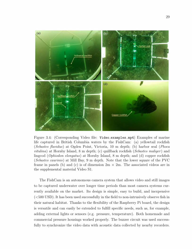
29

Figure 3.4: (Corresponding Video file: Video examples.mp4) Examples of marinelife captured in British Columbia waters by the FishCam: (a) yellowtail rockfish(Sebastes flavidus) at Ogden Point, Victoria, 10 m depth; (b) harbor seal (Phocavitulina) at Hornby Island, 8 m depth; (c) quillback rockfish (Sebastes maliger) andlingcod (Ophiodon elongatus) at Hornby Island, 8 m depth; and (d) copper rockfish(Sebastes caurinis) at Mill Bay, 9 m depth. Note that the lower square of the PVCframe in panels (b) and (c) is of dimension 2m × 2m. The associated videos are inthe supplemental material Video S1.

The FishCam is an autonomous camera system that allows video and still images

to be captured underwater over longer time periods than most camera systems cur-

rently available on the market. Its design is simple, easy to build, and inexpensive

(<500 USD). It has been used successfully in the field to non-intrusively observe fish in

their natural habitat. Thanks to the flexibility of the Raspberry Pi board, the design

is versatile and can easily be extended to fulfill specific needs, such as, for example,

adding external lights or sensors (e.g. pressure, temperature). Both homemade and

commercial pressure housings worked properly. The buzzer circuit was used success-

fully to synchronize the video data with acoustic data collected by nearby recorders.

30

Figure 3.5: (Corresponding audio file: buzzer sequence.wav) Waveform (top) andspectrogram (bottom) of a 3 kHz-tone sequence from the FishCam received by ahydrophone located 3 m away. The sampling frequency of the acoustic recorder was32 kHz. The spectrogram was computed by Fast Fourier Transform using 512-sampleHanning windows overlapped at 95%.

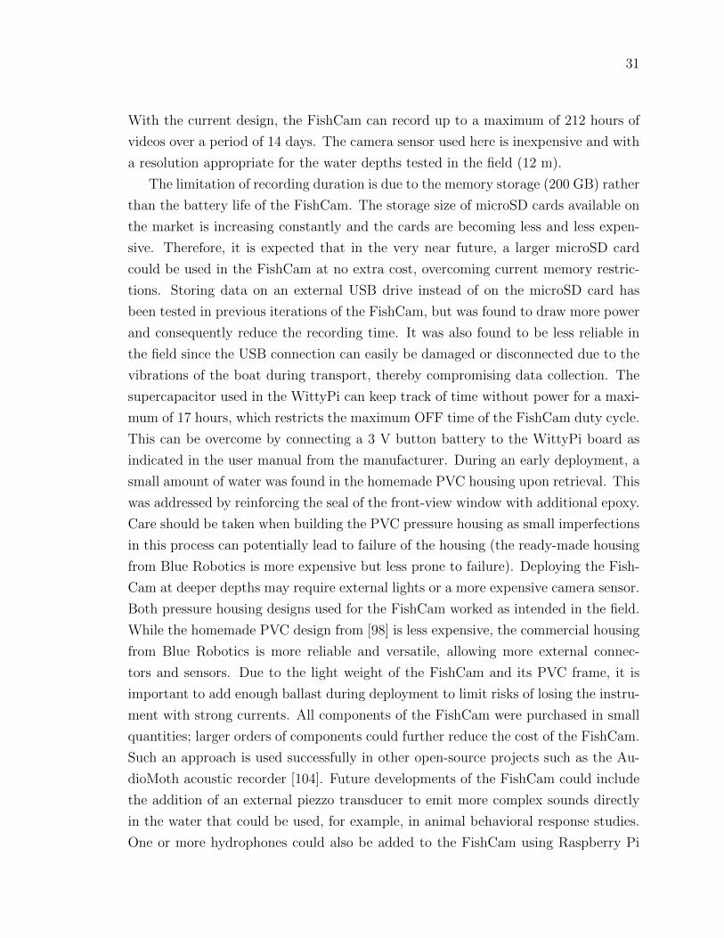
31

With the current design, the FishCam can record up to a maximum of 212 hours of

videos over a period of 14 days. The camera sensor used here is inexpensive and with

a resolution appropriate for the water depths tested in the field (12 m).

The limitation of recording duration is due to the memory storage (200 GB) rather

than the battery life of the FishCam. The storage size of microSD cards available on

the market is increasing constantly and the cards are becoming less and less expen-

sive. Therefore, it is expected that in the very near future, a larger microSD card

could be used in the FishCam at no extra cost, overcoming current memory restric-

tions. Storing data on an external USB drive instead of on the microSD card has

been tested in previous iterations of the FishCam, but was found to draw more power

and consequently reduce the recording time. It was also found to be less reliable in

the field since the USB connection can easily be damaged or disconnected due to the

vibrations of the boat during transport, thereby compromising data collection. The

supercapacitor used in the WittyPi can keep track of time without power for a maxi-

mum of 17 hours, which restricts the maximum OFF time of the FishCam duty cycle.

This can be overcome by connecting a 3 V button battery to the WittyPi board as

indicated in the user manual from the manufacturer. During an early deployment, a

small amount of water was found in the homemade PVC housing upon retrieval. This

was addressed by reinforcing the seal of the front-view window with additional epoxy.

Care should be taken when building the PVC pressure housing as small imperfections

in this process can potentially lead to failure of the housing (the ready-made housing

from Blue Robotics is more expensive but less prone to failure). Deploying the Fish-

Cam at deeper depths may require external lights or a more expensive camera sensor.

Both pressure housing designs used for the FishCam worked as intended in the field.

While the homemade PVC design from [98] is less expensive, the commercial housing

from Blue Robotics is more reliable and versatile, allowing more external connec-

tors and sensors. Due to the light weight of the FishCam and its PVC frame, it is

important to add enough ballast during deployment to limit risks of losing the instru-

ment with strong currents. All components of the FishCam were purchased in small

quantities; larger orders of components could further reduce the cost of the FishCam.

Such an approach is used successfully in other open-source projects such as the Au-

dioMoth acoustic recorder [104]. Future developments of the FishCam could include

the addition of an external piezzo transducer to emit more complex sounds directly

in the water that could be used, for example, in animal behavioral response studies.

One or more hydrophones could also be added to the FishCam using Raspberry Pi

32

compatible sound acquisition boards [105]. The FishCam could find applications in

a wide range of aquatic research. Many marine ecology research studies use baited

remote underwater video (BRUV) to record fish diversity, abundance, and behaviour

[85]. Many of these BRUVs typically have an autonomy of fewer than 10 hours [106,

107]. A FishCam could be used in BRUV studies to expand the duration and spatial

coverage of the monitoring effort. FishCams deployed in pairs could potentially be

used as stereo-video systems for accurate fish size measurements [108, 109], although

this may require the use of a different lens.

Advances in technology, along with the increasing popularity of open-source sys-

tems and software, allow researchers to build sophisticated research instruments at

lower costs. These innovations can then be made accessible to a much broader de-

mographic. Through this approach, new instruments are becoming available to the

marine research community to monitor underwater environments over longer peri-

ods of time, over greater spatial scales, and at a minimal cost. Advanced electronic

components, such as those used in the FishCam, become not only more accessible

to the research community, but also to the general public. This encourages citizen

science initiatives that have the potential to improve and expand ongoing research

by scientists [110]. Our vision for the FishCam is to have applications in education,

citizen science and ecological research. The FishCam could be built by students to

teach them the basics of electronics, programming and environmental science, and

used in deployments by citizen scientists, including recreational divers and students,

to acquire data to be analyzed by researchers to address ecologically-important ques-

tions. Such an approach offers a unique opportunity to engage with students and

local communities to learn new skills that contribute directly to real-world research

and conservation [111–113].

3.5 Summary

Capabilities of FishCam:

Maximum video capacity of 212 hours over a period of 14 days.

Duty cycles fully customizable.

Acquisition of videos and/or pictures.

Large field of view (110).

33

Wireless access and configuration.

Possibility to add external sensors.

Inexpensive and easy to build.

Limitations of FishCam:

Needs additional external lights for deployment in deep water.

Basic electronics skills required (i.e., soldering).


This paper is dedicated to the late Callum Mireault (Memorial University of New-

foundland and CHONe graduate student) who brainstormed ideas with the authors

at early stages of this project. Data collection in the field was made possible thanks

to all the volunteers of the Juanes Lab at the University of Victoria, Scott Trivers,

and Tristan Blaine from the Central Coast Indigenous Resource Alliance (CCIRA).

This research is supported by the Natural Sciences and Engineering Research Council

(NSERC) Canadian Healthy Oceans Network (CHONe) and its partners: Fisheries

and Oceans Canada and INREST (representing the Port of Sept-Iles and City of Sept-

Iles), JASCO Applied Sciences, and NSERC. X.M was also funded by an NSERC

Postgraduate Scholarship and a Mitacs Accelerate Fellowship.

34

Chapter 4

Identifying fish sounds in the wild:

development and comparison of

three audio/video platforms

For this chapter, I designed, built, and tested the audio/video arrays and led the

data collection in the field. Morgan Black, Kieran Cox, and Jessica Qualley led the

diving operations in the field and helped with the identification of fish species in the

video data. I performed the data analysis, implemented the detection and localization

scripts in Python, and created the supporting open-source package ecosound. Dr. Stan

Dosso provided the initial Matlab script to calculate the confidence intervals for the

non-linear localization. I wrote the paper with editorial assistance from Dr. Francis

Juanes and Dr. Stan Dosso.

4.1 Abstract

Fish sounds can be used to non-intrusively detect the presence of fish and potentially

to estimate their number (or density) over large areas and long time periods. How-

ever, many fish sounds have not yet been associated to specific species, which limits

the usefulness of this approach. While recording sounds from individual species can

be performed in tanks, it presents many challenges, including the fact that many fish

do not produce sounds in captivity. This paper proposes three audio/video platforms

capable of identifying species-specific fish sounds in the wild. Each platform is de-

signed with specific habitats and logistical and cost constraint in mind, but all are

35

able to record fish sounds, acoustically localize the fish in three-dimensions (using lin-

earlized or fully non-linear inversion) and record video to identify the fish and observe

their behavior. The first platform, referred to as the large array, is composed of six

hydrophones, an acoustic recorder, and two video cameras secured to a PVC frame

of dimensions 2 m × 2 m × 3 m, that can be transported and assembled in the field.

Despite its higher cost, this array provides the largest field of view, the most accurate

acoustic localization, and is well suited to long-term deployments (weeks). The second

platform, referred to as the mini array, uses a single video camera, four hydrophones,

and an acoustic recorder on a one cubic meter PVC frame. It can be deployed more

easily in constrained locations or on rough/uneven seabed and is less expensive, but

has lower localization capabilities. The third platform, referred to as the mobile array,

consists of four hydrophones connected to an acoustic recorder mounted on a tethered

underwater drone with built-in video. This array allows remote control and real-time

positioning in response to observed fish presence, is easy and inexpensive to deploy

and operate, but has also lower localization capabilities. The three platforms were

deployed at four locations off the east coast of Vancouver Island, British Columbia,

Canada, and allowed the identification and description of sounds from quillback rock-

fish (Sebastes maliger), copper rockfish (Sebastes caurinus), and lingcod (Ophiodon

elongatus). In addition, data collected with the large array provided estimated mean

source levels of 115.4 and 113.5 dB re 1 µPa for lingcod and quillback rockfish sounds,

respectively.

4.2 Introduction

Over 800 species of fishes worldwide are currently known to be soniferous [8, 9, 114].

It is likely that many more species produce sounds, but their repertoires have not

yet been identified. Fishes can produce sound incidentally while feeding or swimming

(e.g., [11, 12]) or intentionally for communication [13, 14]. For example, fish sound

spectral and temporal characteristics can convey information about male status and

spawning readiness to females [15], or male body condition [16]. It has been speculated

that some species of fish may also emit sound to orient themselves in the environment

(i.e., by echolocation [17]). As is the case for marine mammal vocalizations, fish

sounds can typically be associated with a specific species and sometimes to specific

behaviours [14, 18]. Recently, Parmentier et al. [115] used fish sounds to identify a

new cryptic species of humbug damselfish in French Polynesia. It has also been shown

36

that several populations of the same species can have different acoustic dialects [19].

Consequently, researchers can measure the temporal and spectral characteristics of

recorded fish sounds to identify which species of fish are present in the environment,

to infer their behaviour and, in some cases, to potentially identify and track a specific

population [20].

Using passive acoustics to monitor fish can complement existing monitoring tech-

niques such as net sampling [21], active acoustics [22], or acoustic tagging [23]. Passive

acoustics presents several advantages: It is non-intrusive, can monitor continuously

for long periods of time, and can cover large geographical areas. However, in order

to use passive acoustics to monitor fish, their sounds must first be characterized and

catalogued under controlled conditions. This can be achieved in various ways. The

most common way to identify species and behaviour-specific sounds is to capture and

isolate a single fish or several fish of the same species in a controlled environment

(typically a fish tank) and record the sounds they produce (e.g., [24–26]). This ex-

perimental setup precludes sound contamination from other species and allows visual

observation of the behaviour of the animal. While these studies provide important

findings on fish sound production, they do not always result in sounds that fish pro-

duce in their natural environments. To partially address this issue, other studies

record fish in natural environments but constrained in fishing net pens to ensure they

remain in sufficient proximity of the hydrophones (e.g., [28]). This also presents some

challenges as other fish species outside the pen can potentially be recorded.

Passively recording fish in their natural environment has many advantages, espe-

cially in terms of not disrupting the animals. However, it provides less control over

external variables and also presents many technical challenges. Remote operated

vehicles (ROVs) equipped with video cameras and hydrophones have been used by

Sprague and Luczkovich in 2004 [29] and Rountree and Juanes in 2010 [30]. Locas-

cio and Burton deployed fixed autonomous passive acoustic recorders and conducted

diver-based visual surveys to document the presence of fish species [31]. They also

developed customized underwater audio and video systems to verify sources of fish

sounds and to understand their behavioural contexts. Most of these monitoring tech-

niques are limited by high power consumption and data storage space requirements,

and are typically only deployed for short periods of time. Cabled ocean observato-

ries equipped with hydrophones and video cameras provide valuable data for more

extended time periods but by their nature provide data at fixed locations and are

expensive to deploy and maintain [10, 32]. As stated by Rountree et al. in 2006

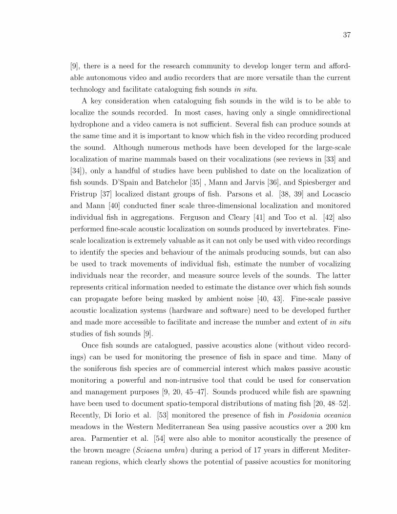
37

[9], there is a need for the research community to develop longer term and afford-

able autonomous video and audio recorders that are more versatile than the current

technology and facilitate cataloguing fish sounds in situ.

A key consideration when cataloguing fish sounds in the wild is to be able to

localize the sounds recorded. In most cases, having only a single omnidirectional

hydrophone and a video camera is not sufficient. Several fish can produce sounds at

the same time and it is important to know which fish in the video recording produced

the sound. Although numerous methods have been developed for the large-scale

localization of marine mammals based on their vocalizations (see reviews in [33] and

[34]), only a handful of studies have been published to date on the localization of

fish sounds. D’Spain and Batchelor [35] , Mann and Jarvis [36], and Spiesberger and

Fristrup [37] localized distant groups of fish. Parsons et al. [38, 39] and Locascio

and Mann [40] conducted finer scale three-dimensional localization and monitored

individual fish in aggregations. Ferguson and Cleary [41] and Too et al. [42] also

performed fine-scale acoustic localization on sounds produced by invertebrates. Fine-

scale localization is extremely valuable as it can not only be used with video recordings

to identify the species and behaviour of the animals producing sounds, but can also

be used to track movements of individual fish, estimate the number of vocalizing

individuals near the recorder, and measure source levels of the sounds. The latter

represents critical information needed to estimate the distance over which fish sounds

can propagate before being masked by ambient noise [40, 43]. Fine-scale passive

acoustic localization systems (hardware and software) need to be developed further

and made more accessible to facilitate and increase the number and extent of in situ

studies of fish sounds [9].

Once fish sounds are catalogued, passive acoustics alone (without video record-

ings) can be used for monitoring the presence of fish in space and time. Many of

the soniferous fish species are of commercial interest which makes passive acoustic

monitoring a powerful and non-intrusive tool that could be used for conservation

and management purposes [9, 20, 45–47]. Sounds produced while fish are spawning

have been used to document spatio-temporal distributions of mating fish [20, 48–52].

Recently, Di Iorio et al. [53] monitored the presence of fish in Posidonia oceanica

meadows in the Western Mediterranean Sea using passive acoustics over a 200 km

area. Parmentier et al. [54] were also able to monitor acoustically the presence of

the brown meagre (Sciaena umbra) during a period of 17 years in different Mediter-

ranean regions, which clearly shows the potential of passive acoustics for monitoring

38

fish at large scales and over long time periods. Finally, Rountree and Juanes [55]

demonstrated how passive acoustics could be used to detect an invasive fish species

in a large river system.

In this chapter, we propose three combinations of audio/video hardware and soft-

ware to catalog and characterize fish sounds in the field.

4.3 Methods

4.3.1 Description of the audio/video arrays

Three audio/video arrays, referred to as large, mini and mobile arrays, were developed

to acoustically localize and visually identify fish producing sounds. Each array was

designed with different constraints in mind. The large array was configured for ac-

curate 3D acoustic localization, the mini array for easier deployments in constrained

locations or on rough/uneven seabeds, and the mobile array for dynamic real-time

spatial sampling over shorter time periods (hours).

Large array

The large array is a static platform deployed on the seafloor that records audio and

video data for one to two weeks.

The large array uses six M36-V35-100 omnidirectional hydrophones (GeoSpectrum

Technologies Inc.) connected to an AMAR-G3R4.3 acoustic recorder (JASCO Ap-

plied Sciences) with a PVC housing rated to 250 m depth. Four of the hydrophones

(1-4 in Figure 4.1) are connected to the first acquisition board of the recorder via

a 4 m long 4-to-1 spliter cable. The two other hydrophones (5,6 in Figure 4.1) are

connected, via a 3 m long 2-to-1 splitter cable, to the second acquisition board of the

recorder. The recorder is set to acquire acoustic data continuously as 30-min wave

files, at a sampling frequency of 32 kHz, with a bit depth of 24 bit, and with a pre-

digitalization analog gain of 6 dB. An external battery pack with 48 D-cell batteries

is used to power the recorder, which, using this configuration, allows the system to

acquire data for up to 35 days. An end-to-end calibration was performed for each hy-

drophone using a piston-phone type 42AA precision sound source (G.R.A.S. Sound &

Vibration A/S) at 250 Hz. System gain measured on all hydrophones was −167.3±0.2

dB re FS/µPa, where FS is the full digitalization scale (i.e., amplitudes values be-

tween −1 and 1). Positions of the hydrophones within the large array (Figure 4.1)

39

Figure 4.1: Large array. (a) Photograph of the large array deployed in the field.(b) side view and (c) top view diagrams of the array with dimensions. The sixhydrophones are represented by the numbered gray circles. The top and side videocameras are indicated by C1 and C2, respectively. Note that C1 is not represented in(c) for clarity. The acoustic recorder and its battery pack are indicated by AR andPB, respectively. Gray and red lines represent the PVC structure of the array (redindicating the square base of the array).

.

were defined to maximize the accuracy of the acoustic localization (see optimization

procedure described in section 4.3.6).

Two autonomous FishCam cameras [84] are used to record video inside the large

array. One (C1) is located at the top of the array and is oriented downward towards

the sea bottom, and the other (C2) is located on the side of the array, pointing

horizontally towards hydrophone 4 (Figure 4.1). Each camera is set to record video

continuously during the day (from 5:00 to 21:00 local time) and to shut-down during

the night. Video data are recorded on 300-s h264 files, with a frame rate of 10 frames

per second, a resolution of 1600 × 1200 pixels, and an ISO of 400. Both cameras emit

different sequences of beeps at 3 kHz every 4 hours for time-synchronizing the video

and acoustic data. The autonomy of the FishCams is storage-limited, dependent on

the underwater light conditions, and typically ranges from 8 to 14 days (see [84]).

All instruments are secured to a tent-shaped PVC frame of 2 m width, 2 m length

and 3 m height (Figure 4.1). The frame is built out of schedule 40 1 1/2” PVC

pipes, and 4-way and 3-way Formufit PVC Tee fittings. The core components of the

frame that support most of the weight from the acoustic recorder are glued together

with PVC cement. Other parts of the frame are snug-fit to allow the array to be

disassembled. Two galvanized crossed 1/8” wire cables with turnbuckles are used

on two sides of the array to add rigidity to the frame. Two ropes with galvanized

thimbles are attached at the top of the PVC frame to lower or lift the array to/from

40

the seafloor during deployment and recovery. The acoustic recorder (AR) and its

battery pack (BP) are supported by two schedule 80 1 1/2” PVC pipes located at

the base of the array (red solid lines in Figure 4.1b,c) and secured with Smart Band

fasteners (HCL Fasteners Ltd). Hydrophones are held snug in a 3/4” 3/4” 1/2” PVC

tee fitting that is connected successively to a 1/2” PVC nipple, a 1 1/2” 1/2” PVC

bush, and a 1 1/2” 3-way Formufit PVC Tee fitting cut in half and secured to the array

frame using stainless steel hose clamps. Cables from the recorder to the hydrophones

are held to the PVC frame using re-usable self-gripping Velcro bands. Cameras are

attached to the frame with PVC union fittings as described in [84]. Camera C1 is at

the top of the main PVC structure and camera C2 is on a separate PVC frame that

is clipped on the side of the main structure during deployment.

Mini array

Like the large array, the mini array is a static platform deployed on the seafloor that

records audio and video data for one to two weeks, but has a much smaller footprint

than the large array.

The mini array uses four HTI-96-MIN omnidirectional hydrophones (High Tech

Inc.) connected to a SoundTrap ST4300HF acoustic recorder (Ocean Instruments,

New Zealand). The recorder is set to acquire temperature every 10 s, and acoustic

data continuously on 15-min wave files, at a sampling frequency of 48 kHz, and with

a bit depth of 16 bit. Using this configuration the recorder has an autonomy of

approximately 6 days. An end-to-end calibration was performed for each hydrophone

using a piston-phone type 42AA precision sound source (G.R.A.S. Sound & Vibration

A/S) at 250 Hz. System gain measured on all hydrophones was −168.2 ± 0.2 dB re

FS/µPa. Coordinates of the hydrophones are indicated in Figure 4.2.

The mini array uses a single FishCam video camera facing horizontally and placed

below the four hydrophones. It is set to record video using the same configuration

used for the large array.

The recorder, hydrophones, and camera are secured to a frame of 1.2 m width, 1.3

m length and 1.3 m height (Figure 4.2). It is built out of a combination of schedule 40

1 1/2” PVC pipe (light gray lines in Figure 4.2) and 3/4” high density polyethylene

(HDPE) pipe (black lines in Figure 4.2). PVC and HDPE sections of the frame

are assembled using 4-way or 3-way PVC and polyethylene fittings. The camera is

attached to the frame with PVC union fittings and the acoustic recorder with zip

41

Figure 4.2: Mini audio and video array. (a) Photograph of the mini array beforedeployment in the field. (b) rear view and (c) top view diagrams of the mini arraywith dimensions. The four hydrophones are represented by the numbered gray circles.The camera and the acoustic recorder are indicated by C and AR, respectively. Greyand black lines represent the frame of the array.

.

ties and duct tape. Hydrophones are placed at the end of each HDPE sections of the

frame and secured with Velcro bands.

Mobile array

Unlike the static large and mini arrays, the mobile array is remote controlled, can be

re-positioned dynamically in the environment in response to observed fish presence,

and can collect audio and video data over periods of approximately two hours.

The mobile array uses a SoundTrap ST4300HF acoustic recorder (Ocean Instru-

ments, New Zealand) with four HTI-96-MIN omnidirectional hydrophones (High Tech

Inc.) secured on top of a Trident (Sofar Ocean Technologies) underwater drone (Fig-

ure 4.3). The recorder is set to acquire temperature every 10 s, and acoustic data

continuously on 15-min wave files, at a sampling frequency of 48 kHz, and with a bit

depth of 16 bit. Both the recorder and hydrophones are the same ones used for the

mini array, and thus the system gain is the same (i.e., −168.2 ± 0.2 dB re FS/µPa).

The Trident underwater drone uses a 100 m tether and is controlled by a JXD

S192K gaming tablet (JinXing Digital Co. Ltd) connected via WiFi to the Trident

surface hub. Video from the drone’s camera is transmitted in real-time to the JXD

controller and is recorded with a resolution of 1920 × 1080 pixels and a frame rate of

30 frames per second. Time, water temperature, depth and horizontal orientation of

42

Figure 4.3: Mobile audio and video array. (a) Photograph of the mobile array de-ployed in the field. (b) rear view and (c) top view diagrams of the mobile arraywith dimensions. The four hydrophones are represented by the numbered gray cir-cles. The underwater drone and the acoustic recorder are indicated by ROV andAR, respectively. The video camera is located at the front of the drone (coordinates:(0,0.2,−0.05)) facing forward. Black lines represent the frame of the array.

the drone are recorded and displayed on each video recording. The hydrophones and

recorder are attached to a small frame made of 3/4” HDPE pipe, 3-way polyethylene

fittings and zip ties, and secured to the bottom of the drone using four M3 screws.

Hydrophones are secured to the frame using Velcro bands and are placed at the end

of each arm of the frame that extend to approximately 0.5 m on each side, in front,

and above the drone (Figure 4.3). Two 10 cm long vertical pieces of HDPE pipe

are placed at the bottom-front of the frame to keep the drone and thrusters out

of the sand and mud when resting on the seafloor. Pieces of buoyant polyethylene

foam are attached with zip ties on several sections of the frame to maintain balance

and buoyancy. The array is made slightly negatively buoyant to remain stable when

resting on the seafloor with the thrusters turned off.

4.3.2 Automatic detection of acoustic transients

Data collected by the audio/video arrays are analyzed in four steps. First, acoustic

transients are automatically detected on the signal from one of the hydrophones (this

section). Second, the time-difference of arrivals (TDOAs) between hydrophones of the

array are estimated via cross-correlation (section 4.3.3). Third, the 3D localization

of the detected events is estimated (section 4.3.4) using linearized inversion (for the

large array) or full non-linear inversion (for the mini and mobile array). Finally, 3D

acoustic localizations are matched with the video recordings to identify the species

and behavior of the fish that emitted for the sound (section 4.3.5).

43

All acoustic events (including, but not limited to fish sounds) are automatically

detected on data from one of the hydrophones of the array (hydrophone 4 for the

large array, Figure 4.1, and hydrophone 2 for the mini and mobile arrays, Figures 4.2

and 4.3). The detection is performed by calculating and denoising the spectrogram,

then by segmenting the denoised spectrogram to identify acoustic transients.

The spectrogram is calculated using 0.0625 s frames with time steps of 0.01 s and

0.0853 s FFTs. Given that most fish sounds reported in the literature have a peak

frequency below 5 kHz [77, 116], the spectrogram is truncated to only keep frequencies

from 0 to 6 kHz. Magnitude values are squared to obtain energy and expressed in

decibels. To improve the signal-to-noise ratio of fish sounds and attenuate tonal

sounds from vessels, the spectrogram is equalized using a median filter, calculated

with a sliding window, for each row (frequency) of the spectrogram. The equalized

spectrogram, S[t, f ], at each time bin, t, and frequency bin, f , is calculated as

S[t, f ] = S[t, f ] − Smed[t, f ], (4.1)

where S[t, f ] is the original spectrogram and Smed[t, f ] is the median spectrogram

calculated as:

Smed[t, f ] = median(S[t−k, f ], S[t−k+1, f ], . . . , S[t, f ], . . . , S[t+k−1, f ], S[t+k, f ]),

(4.2)

where the median is calculated on a window centered on the tth sample and has a

duration of 2k+1 bins. Here, we choose a median window equivalent to a 3 s duration

(k = 150), which removes constant tonal components from vessels without removing

the longer grunting sounds from fish.

Once the spectrogram is calculated and equalized, it is segmented by calculating

the local energy variance on a two-dimensional (2D) kernel of size ∆T × ∆F . The

resulting matrix, Svar, is defined as

Svar[t, f ] =1

(∆T∆F ) − 1

t+∆T2∑

i=t−∆T2

f+∆F2∑

j=f−∆F2

|S[i, j] − µ|2, (4.3)

44

where µ is the mean over the 2D kernel

µ =1

(∆T∆F )

t+∆T2∑

i=t−∆T2

f+∆F2∑

j=f−∆F2

S[i, j]. (4.4)

The number of time and frequency bins of the kernel are chosen to be equivalent to

0.1 s and 300 Hz, respectively. Bins of the spectrogram with a local variance less

than 20 were set to zero and all the other bins were set to one. Bounding boxes of

contiguous bins in the binarized spectrogram are then defined using the outer border

following algorithms described in [117]. These bounding boxes define the start and

stop times and the minimum and maximimum frequency of the acoustic events to

localize.

4.3.3 Time Difference of Arrival

The TDOAs are obtained by cross-correlating acoustic events detected on the record-

ing from the reference-hydrophone with the recordings from the other hydrophones.

Before performing the cross-correlation, each recording is band-pass filtered in the

frequency band determined by the detector using an eighth-order zero-phase forward-

backward Butterworth filter [118], and up-sampled using the FFT method [119], to

obtain a time resolution of 0.1 µs. The TDOA of a detected signal between a pair

of hydrophones is defined as the time of the maximum peak in the normalized cross-

correlation within the range of possible values for the array (i.e., ±1.9 ms for the large

array, ±0.8 ms for the mini array, and ±0.6 ms for the mobile array). Only TDOAs

with a peak correlation amplitude greater than 0.5 are considered for localization.

4.3.4 Acoustic localization

The forward model

Given that fish sounds only propagate over small distances [82] and that hydrophones

of the audio/video arrays are separated by less than 3 m, it is assumed for the local-

ization, that the effects of refraction are negligible and that the sound velocity, v, is

constant (here, v = 1484 m/s). In such case, the TDOA ∆tij between hydrophones i

45

and j is defined by

∆tij =1

v

(√(X − xi)2 + (Y − yi)2 + (Z − zi)2 −

√(X − xj)2 + (Y − yj)2 + (Z − zj)2

),

(4.5)

where x, y, z are the known 3D Cartesian coordinates of hydrophones i and j relative

to the array center, and X, Y , Z are the unknown coordinates of the acoustic source

(M = 3 unknowns).

Localizing the acoustic source is a non-linear problem defined by

dk; k = 1, N = d = d(m) (4.6)

where, d represents the N measured TDOA data and d(m) the modeled TDOA data

with m = [X, Y, Z]T (in the common convention adopted here bold lower-case symbols

represent vectors and bold upper-case symbols represent matrices). The large array

has 6 hydrophones and can provide 5 independent TDOAs measurements (N = 5),

while the mini and mobile arrays have 4 hydrophones which provide 3 independent

TDOA measurements (N = 3).

Linearized inversion

Acoustic localization for the large array is performed using linearized inversion. The

localization problem in Eq. 4.6 can be linearized by starting at a location m0, and

iteratively solving for small perturbations δm, of the model m [76]. Assuming errors

on the data are identical and independently Gaussian-distributed random variables,

the maximum-likelihood solution is

δm =[ATA

]−1AT δd, (4.7)

where δd = d − d(m0), and A is the N ×M Jacobian matrix of partial derivatives

with elements

Aij =∂di(m0)

∂mj

; i = 1, ..., N ; j = 1, ...,M. (4.8)

The location m of the acoustic source can be estimated by solving for δm and re-

defining iteratively

ml+1 = ml + αδm; l = 0, ..., L; 0 < α ≤ 1, (4.9)

46

until convergence (i.e., until ∥ml+1 − ml∥2 < 0.01 m). In Eq. 4.9, α is a stepsize

damping factor (here, α = 0.1) and L is the maximum number of iterations (here,

L = 100). The localization uncertainties, about the final solution, are estimated from

the diagonal elements of the model covariance matrix Cm defined by

Cm = σ2[ATA

]−1, (4.10)

where σ2 is the variance of the TDOA measurement errors. The localization process is

repeated for each detected sound by choosing five different starting models m0. One

is always selected at the center of the array (i.e., m0 = [0, 0, 0]T ), and the four others

are randomly drawn from a uniform distribution within the volume of the array. The

localization result with the smallest data misfit is considered the best solution. The

variance of the TDOA measurement errors, σ2 in Eq. 4.10, is estimated for each

localization by

σ2 =1

N − 3

N∑i−1

(di − di(m))2 . (4.11)

Non-linear inversion

The spacing between hydrophones for the mini and mobile arrays is smaller than for

the large array and most sound sources to localize are outside the volume of the array.

In such cases the problem becomes highly non-linear and localizing using linearized

inversion is less appropriate, as it has difficulties converging towards a final solution

and the linearized uncertainty estimates become unreliable. Consequently, acoustic

localization for the mini and mobile arrays is performed using a fully non-linear inver-

sion. A 3D spatial search grid of pre-computed time-difference data, d(m) is defined

using Eq. 4.5 and simulated sound sources positioned every 2 cm from −3 m to 3

m in the x and y axes, and from −1 m to 3 m in the z axis (coordinate systems

defined in Figures 4.2 and 4.3). Assuming errors in the data are identical and inde-

pendently Gaussian distributed, the un-normalized likelihood L(m, σ) is estimated

at each location m of the search grid as

L(m, σ) = exp

[− 1

2σ2|d− d(m)|2

], (4.12)

where |d − d(m)|2 =∑N

i=1(di − di(m))2, and σ2 is the variance of the TDOA mea-

surement errors estimated at the grid location mML that minimizes |d − d(m)|2.

47

The likelihood values of the Mx × My × Mz grid are then normalized by S =∑Mx

i=1

∑My

j=1

∑Mz

k=1 L(xi, yj, zk) to obtain a normalized posterior probability density in

3D. The location mML has the maximum likelihood and is considered as the estimate

of the sound source location. Uncertainties of the localization are then characterized

as the limits of the 99% highest-probability density credibility interval of the marginal

probability distributions, Px, Py, and Pz defined for each axis, x, y, and z of the 3D

grid, respectively. As the mini and mobile array can only provide 3 TDOAs, σ2 is

not updated for each localization, as for the large array, but for groups of 3 or more

consecutive localizations and assumed constant over the recording analyzed.

4.3.5 Identification of the localized sounds

Acoustic recordings are automatically analyzed using the process described above

and only acoustic localizations that are within the field of view of the video cameras,

and have uncertainties in each dimension less than 1 m, are kept for further analysis.

Video recordings corresponding to the time of the selected localizations are manually

inspected and experienced taxonomists visually identify individual fish matching the

position of the acoustic localization. Identification is performed to the species level

and when possible the sounds are associated to specific behaviors. Synchronization

beeps emitted by the video cameras are identified in the audio data and used to ensure

the video and audio data are time-aligned properly.

4.3.6 Optimization of hydrophone placement

For the large array, the placement of the hydrophones was defined so as to minimize

the overall localization uncertainty. This was achieved using the simulated annealing

optimization algorithm [120] and followed the procedure developed in [121]. The

optimization consisted of finding the x, y, and z coordinates of the six hydrophones

(18 parameters) that minimizes the average localization uncertainty of 500 simulated

sound sources placed on a 2 m radius sphere around the center of the array. For

a given hydrophone configuration m, the average localization uncertainty, E(m) is

defined as

E(m) =S∑

s=1

√σ2sx + σ2

sy + σ2sz/S, (4.13)

where S is the number of simulated sound sources (S = 500), and σ2sx , σ2

sy , and σ2sz are

the variances of the localization uncertainties of the simulated sound source s in the

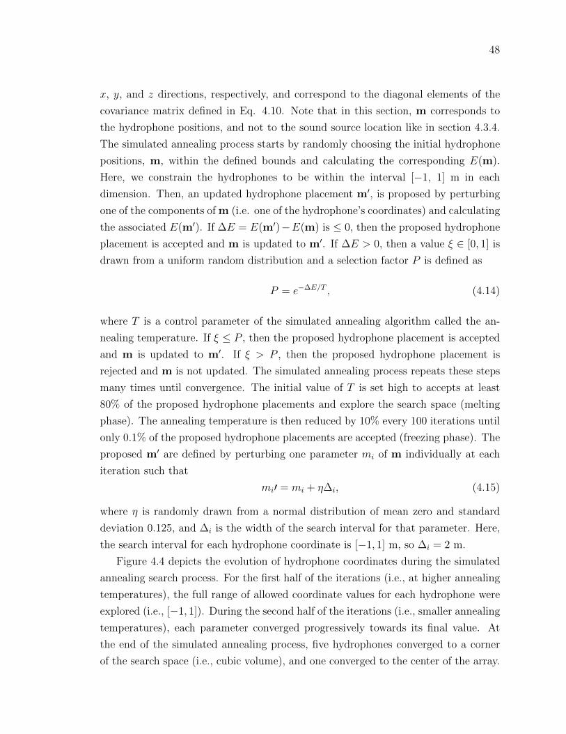
48

x, y, and z directions, respectively, and correspond to the diagonal elements of the

covariance matrix defined in Eq. 4.10. Note that in this section, m corresponds to

the hydrophone positions, and not to the sound source location like in section 4.3.4.

The simulated annealing process starts by randomly choosing the initial hydrophone

positions, m, within the defined bounds and calculating the corresponding E(m).

Here, we constrain the hydrophones to be within the interval [−1, 1] m in each

dimension. Then, an updated hydrophone placement m′, is proposed by perturbing

one of the components of m (i.e. one of the hydrophone’s coordinates) and calculating

the associated E(m′). If ∆E = E(m′)−E(m) is ≤ 0, then the proposed hydrophone

placement is accepted and m is updated to m′. If ∆E > 0, then a value ξ ∈ [0, 1] is

drawn from a uniform random distribution and a selection factor P is defined as

P = e−∆E/T , (4.14)

where T is a control parameter of the simulated annealing algorithm called the an-

nealing temperature. If ξ ≤ P , then the proposed hydrophone placement is accepted

and m is updated to m′. If ξ > P , then the proposed hydrophone placement is

rejected and m is not updated. The simulated annealing process repeats these steps

many times until convergence. The initial value of T is set high to accepts at least

80% of the proposed hydrophone placements and explore the search space (melting

phase). The annealing temperature is then reduced by 10% every 100 iterations until

only 0.1% of the proposed hydrophone placements are accepted (freezing phase). The

proposed m′ are defined by perturbing one parameter mi of m individually at each

iteration such that

mi′ = mi + η∆i, (4.15)

where η is randomly drawn from a normal distribution of mean zero and standard

deviation 0.125, and ∆i is the width of the search interval for that parameter. Here,

the search interval for each hydrophone coordinate is [−1, 1] m, so ∆i = 2 m.

Figure 4.4 depicts the evolution of hydrophone coordinates during the simulated

annealing search process. For the first half of the iterations (i.e., at higher annealing

temperatures), the full range of allowed coordinate values for each hydrophone were

explored (i.e., [−1, 1]). During the second half of the iterations (i.e., smaller annealing

temperatures), each parameter converged progressively towards its final value. At

the end of the simulated annealing process, five hydrophones converged to a corner

of the search space (i.e., cubic volume), and one converged to the center of the array.

49

The simulated annealing process was repeated five times (using a different initial

hydrophone placement) and always led to the same relative hydrophone geometry

(with possible rotations around the center of the array). For practical reasons (i.e.,

restriction in cable length), the hydrophone placement used for the large array (Figure

4.1) is a rotated version of the hydrophone placement shown in Figure 4.4.

Figure 4.4: Optimization of hydrophone placement using simulated annealing: X (toprow), Y (middle row), and Z (bottom row) coordinates of each hydrophone (columns)at each iteration of the simulated annealing process.

Figure 4.5, shows that for the same array footprint (i.e., 2 m × 2 m, Figure 4.5a,b),

the spatial capacity of the large array to localize with an uncertainty below 50 cm is

more than seven times larger than the hydrophone array used in [76] (i.e., 4.2 m3 vs

33.5 m3). This means that fish sounds can be localized accurately even when the fish

are located up to a meter outside the array. The simulated annealing approach was

not used for the mini and mobile arrays as the placement of the hydrophones was

mostly dictated by the mechanical constraints of these platforms.

4.3.7 Characterization of identified fish sounds

Identified fish sounds are characterized by measuring their pulse frequency, pulse

repetition rate, and duration, where a pulse is defined as a positive/negative amplitude

pair. Each fish sound is usually made up of one or more pulses. All measurements

are performed on the waveform as in [122] (Figure 4.6). The pulse period, Tpulse,

50

Figure 4.5: Comparison of localization uncertainties between the large array fromthis study and the array used in [76]. (a) Hydrophone geometry used in [76]. (b)Hydrophone geometry of the large array as defined by the simulated annealing opti-mization process. Estimated 50-cm localization uncertainty isoline of the large array(dashed line) and [76] (solid line) in the (c) XY , (d) XZ, and (e) Y Z plane. Un-certainties for each array were computed using Eq. 4.10 on a 3D grid of 3 m3 withpoints located every 10 cm, and using a standard deviation of data errors of 0.12 ms.

51

is measured as the time separating the two first consecutive amplitude peaks of a

pulse, and is used to calculate the pulse frequency in hertz (i.e., 1/Tpulse). The pulse

repetition interval, Trep, is measured as the duration between the first peak of two

consecutive pulses, and is used to calculate the pulse repetition rate in pulses per

second (i.e., 1/Trep). The duration, Tdur, is the duration of the fish sound in seconds.

There is only one duration measurement per fish sound. However, fish sounds with

multiple pulses (typically grunts), have several measurements of pulse frequency and

pulse repetition rate (e.g., 4.6).

Figure 4.6: Waveform of a fish grunt composed of six pulses. The pulse period, Tpulse,and pulse repetition interval, Trep, are measured on the waveform representation ofthe fish sound to calculate the pulse frequency and pulse repetition rate, respectively.Tdur represents the duration of the sound.

4.3.8 Estimation of source levels

The acoustic source levels are calculated for the localized fish sounds by applying

estimated transmission loss values to the received levels using [123],

SL = RL + PL, (4.16)

where SL is source level RL is received level, and PL is the propagation loss (all in

dB re 1µPa). Received levels are calculated for each fish sound after converting the

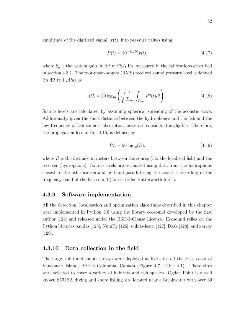
52

amplitude of the digitized signal, x(t), into pressure values using

P (t) = 10−Sg/20x(t), (4.17)

where Sg is the system gain, in dB re FS/µPa, measured in the calibrations described

in section 4.3.1. The root-mean-square (RMS) received sound pressure level is defined

(in dB re 1 µPa) as

RL = 20 log10

(√1

Tdur

∫Tdur

P 2(t)dt

). (4.18)

Source levels are calculated by assuming spherical spreading of the acoustic wave.

Additionally, given the short distance between the hydrophones and the fish and the

low frequency of fish sounds, absorption losses are considered negligible. Therefore,

the propagation loss in Eq. 4.16, is defined by

PL = 20 log10(R), (4.19)

where R is the distance in meters between the source (i.e. the localized fish) and the

receiver (hydrophone). Source levels are estimated using data from the hydrophone

closest to the fish location and by band-pass filtering the acoustic recording in the

frequency band of the fish sound (fourth-order Butterworth filter).

4.3.9 Software implementation

All the detection, localization and optimization algorithms described in this chapter

were implemented in Python 3.8 using the library ecosound developed by the first

author [124] and released under the BSD-3-Clause License. Ecosound relies on the

Python libraries pandas [125], NumPy [126], scikits-learn [127], Dask [128], and xarray

[129].

4.3.10 Data collection in the field

The large, mini and mobile arrays were deployed at five sites off the East coast of

Vancouver Island, British Columbia, Canada (Figure 4.7, Table 4.1). These sites

were selected to cover a variety of habitats and fish species. Ogden Point is a well

known SCUBA diving and shore fishing site located near a breakwater with over 30

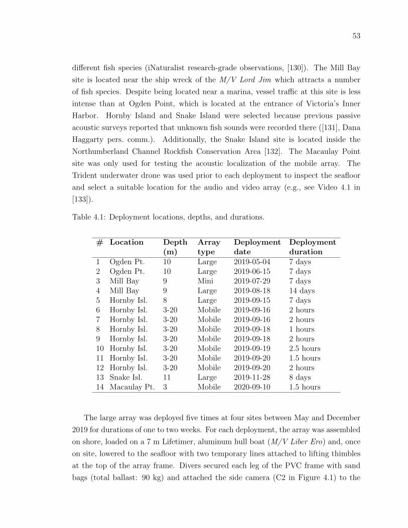
53

different fish species (iNaturalist research-grade observations, [130]). The Mill Bay

site is located near the ship wreck of the M/V Lord Jim which attracts a number

of fish species. Despite being located near a marina, vessel traffic at this site is less

intense than at Ogden Point, which is located at the entrance of Victoria’s Inner

Harbor. Hornby Island and Snake Island were selected because previous passive

acoustic surveys reported that unknown fish sounds were recorded there ([131], Dana

Haggarty pers. comm.). Additionally, the Snake Island site is located inside the

Northumberland Channel Rockfish Conservation Area [132]. The Macaulay Point

site was only used for testing the acoustic localization of the mobile array. The

Trident underwater drone was used prior to each deployment to inspect the seafloor

and select a suitable location for the audio and video array (e.g., see Video 4.1 in

[133]).

Table 4.1: Deployment locations, depths, and durations.

# Location Depth(m)

Arraytype

Deploymentdate

Deploymentduration

1 Ogden Pt. 10 Large 2019-05-04 7 days2 Ogden Pt. 10 Large 2019-06-15 7 days3 Mill Bay 9 Mini 2019-07-29 7 days4 Mill Bay 9 Large 2019-08-18 14 days5 Hornby Isl. 8 Large 2019-09-15 7 days6 Hornby Isl. 3-20 Mobile 2019-09-16 2 hours7 Hornby Isl. 3-20 Mobile 2019-09-16 2 hours8 Hornby Isl. 3-20 Mobile 2019-09-18 1 hours9 Hornby Isl. 3-20 Mobile 2019-09-18 2 hours10 Hornby Isl. 3-20 Mobile 2019-09-19 2.5 hours11 Hornby Isl. 3-20 Mobile 2019-09-20 1.5 hours12 Hornby Isl. 3-20 Mobile 2019-09-20 2 hours13 Snake Isl. 11 Large 2019-11-28 8 days14 Macaulay Pt. 3 Mobile 2020-09-10 1.5 hours

The large array was deployed five times at four sites between May and December

2019 for durations of one to two weeks. For each deployment, the array was assembled

on shore, loaded on a 7 m Lifetimer, aluminum hull boat (M/V Liber Ero) and, once

on site, lowered to the seafloor with two temporary lines attached to lifting thimbles

at the top of the array frame. Divers secured each leg of the PVC frame with sand

bags (total ballast: 90 kg) and attached the side camera (C2 in Figure 4.1) to the

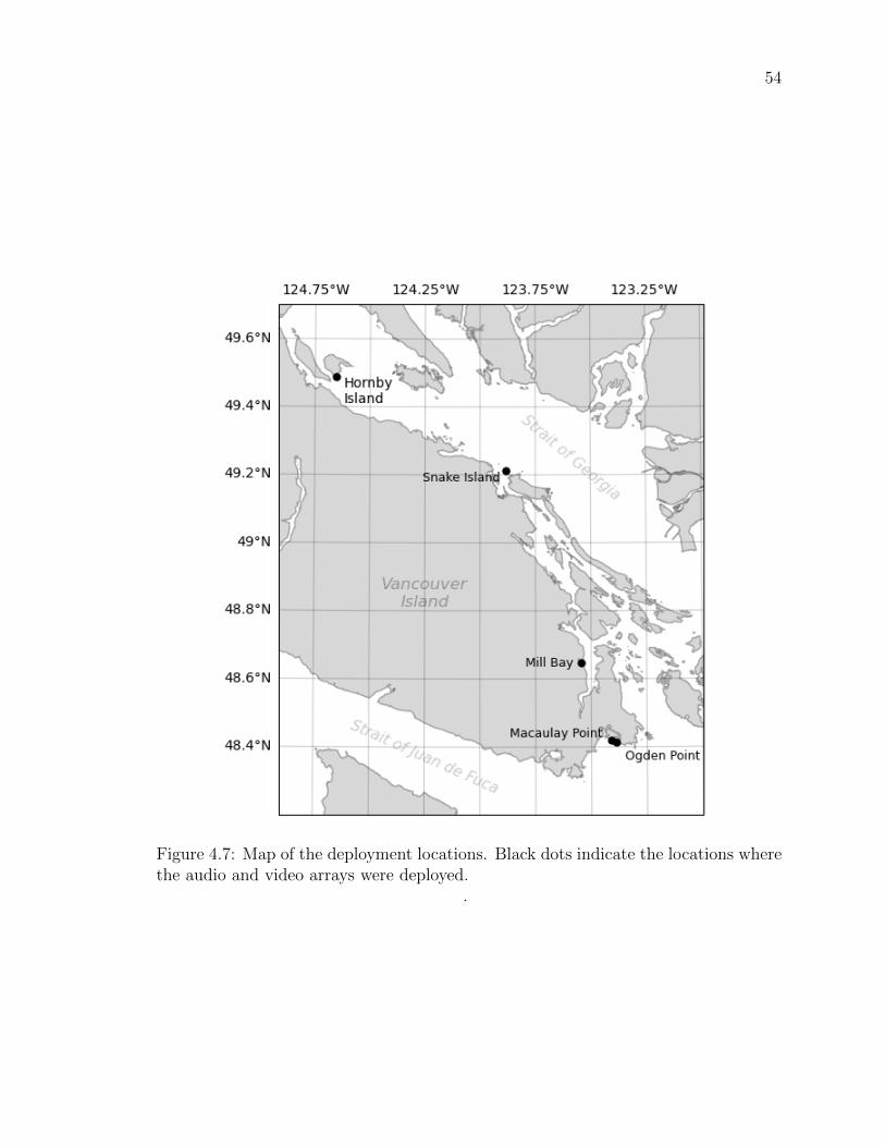
54

Figure 4.7: Map of the deployment locations. Black dots indicate the locations wherethe audio and video arrays were deployed.

.

55

main frame. Deployment operations for the large array required 1 boat driver, 1 dive

tender, 1 deck-hand, and 3 SCUBA divers.

The mini array was deployed once at Mill Bay, in August 2019, for 14 days. The

array was assembled on shore and deployed from a 3.3 m × 1.5 m inflatable boat

(Intex Mariner 4). Divers lowered the mini array to the seafloor by hand and secured

it in place with sand bags (total ballast: 40 kg). Deployment operations for the mini

array required 1 boat driver, 1 dive tender, and 2 SCUBA divers.

The mobile array was deployed seven times between September 16 and 20, 2019

off Hornby Island and once at Macaulay Point in September 2020. The duration of

each deployment was between 1 and 2.5 hours and was dictated by the battery life

of the Trident underwater drone. The mobile array was deployed and piloted from

a 3.3 m × 1.5 m inflatable boat (Intex Mariner 4). Deployments typically consisted

of 1) anchoring the boat with a small weight, 2) deploying the mobile array in the

water, 3) piloting the drone to explore the area to find fish, and 4) land the array on

the seafloor or on rocks to quietly record fish sounds (see Video 4.2 in [133]). This

sequence was repeated several times for each deployment. The choice of locations to

land the array was made based on the video footage only as the acoustic data are

not accessible in real-time. The deployment at Macaulay Point was performed from

a public dock and therefore did not require a boat. Deployment operations for the

mobile array required a single person to drive the boat (when the measurements were

not done from shore) and pilot the underwater drone.

For all three arrays, data were downloaded after recovery of the instruments and

processed in post analysis.

4.3.11 Localization of controlled sound sources in the field

For each array, the accuracy of the acoustic localization was tested in the field using

a source emitting known sounds at a known location.

For the large and mini arrays, the Trident underwater drone was used as the con-

trolled sound source. The characteristic noise from the drone’s thrusters was received

by all hydrophones and was used for localization. The accuracy of the localization

was then assessed when the drone was within the field of view of the cameras. Figure

4.8 shows the acoustic localization of the underwater drone over 6 s as it approaches

the large array. The broadband sounds from the drone’s thrusters (Figure 4.8a) were

localized on the left side of the array at approximately 1 m from the seafloor and with

56

estimated localization uncertainties less than 20 cm in each dimension (Figure 4.8b,c).

These acoustic localizations corresponded closely to positions and movements of the

underwater drone recorded on the video camera C2 (Figure 4.8d,e).

Figure 4.9 shows the acoustic localization of the underwater drone over 6 s as

it faces the mini array. The broadband sounds from the drone’s thrusters (Figure

4.9a) were localized in front of the mini array at approximately 1.5 m above the

seafloor. Localization uncertainties were small along the x and z axes (i.e., less than

10 cm and 50 cm, respectively) but larger along the y axis (up to 2.5 m). The acoustic

localization was successful at determining the bearing and elevation of the underwater

drone but was less accurate at estimating the range.

For the mobile array, the acoustic localization was tested by emitting sounds

from an acoustic projector. A Lubel Labs LL96 acoustic projector was connected

to a Clarion Marine APX280M power amplifier and an Apple Ipod audio player,

and was deployed on the seafloor, in 3 m of water, off a marina dock at Macaulay

Point (Figure 4.7). The mobile array was also deployed on the seafloor and was

located approximately 1 m in front of the projector. The acoustic projector was set

to play a series of fish sounds that were then localized by the mobile array. To test

the localization in different directions, measurements were repeated with the mobile

array oriented at different angles from the acoustic projector (0, 90, 180, and 270).

The orientation of the mobile array and its distance from the source were adjusted

using the compass readings from the drone and visually from the surface. Figure

4.10 shows the localization results from this experiment. As for the mini array, the

localization from the mobile array can resolve the source bearing and elevation angles

relatively well, but is much less accurate at estimating range.

4.4 Results

This section shows examples of fish sounds that were identified in the field using

each platform. Videos corresponding to Figures 4.11-4.16 can be found on this thesis’

online data repository [133].

4.4.1 Identification of fish sounds using the large array

Figure 4.11 shows the acoustic localization of fish sounds over a 10-s period when a

lingcod (Ophiodon elongatus) swam inside the array from the left (Figure 4.11d) and

57

Figure 4.8: Acoustic localization of the underwater drone using the large array de-ployed at Ogden Point (17 Jun. 2019). (a) Spectrogram of the acoustic recordingacquired by hydrophone 4 (frame: 0.0624 s, FFT: 0.0853 s, step size: 0.01 s, Hanningwindow). Beige boxes indicate the time and frequency limits of the sounds that wereautomatically detected. Dots at the top of the spectrogram indicate the colors asso-ciated to the start time of each detection (see color scale on the x-axis) and used forthe localization. Colored camera icons indicate the time of the camera frames shownin panels (d) and (e). (b) Side and (c) top view of the large array. Colored dots andlines represent the coordinates and uncertainty (standard deviation) of the acousticlocalizations, respectively. (d) Image taken by video camera C2 at t = 1.2 s, and (e)t = 5 s, showing the underwater drone approaching the array. Numbers in panels (b),(c), (d), and (e) correspond to the hydrophone identification numbers.

58

Figure 4.9: Acoustic localization of the underwater drone using the mini array de-ployed at Mill Bay (1 Aug. 2019). (a) Spectrogram of the acoustic recording acquiredby hydrophone 2 (frame: 0.0624 s, FFT: 0.0853 s, step size: 0.01 s, Hanning win-dow). Beige boxes indicate the time and frequency limits of the underwater dronesounds that were automatically detected. Dots at the top of the spectrogram indi-cate the colors associated to the start time of each detection (see color scale on thex-axis) and used for the localization. The green camera icon indicates the time ofthe camera frames showed in panels (d) and (e). (b) Rear and (c) top view of themini array. Colored dots and lines represent the coordinates and uncertainty (99%highest-probability density credibility interval) of the acoustic localizations, respec-tively. (d) Image taken by the underwater drone at t = 4.7 s showing the mini array.(e) Image taken from the video camera of the mini array at t = 4.7 s, showing theunderwater drone in front of the array.

59

Figure 4.10: Localization of an acoustic projector using the mobile array deployed atMacaulay Point (10 Sep. 2020). (a) Spectrogram of the acoustic recording acquiredby hydrophone 2 (frame: 0.0624 s, FFT: 0.0853 s, step size: 0.01 s, Hanning window).Beige boxes indicate the time and frequency limits of the fish sounds that were emit-ted by the acoustic projector and automatically detected. (b) Rear and (c) top viewof the mobile array. Colored dots and lines represent the coordinates and uncertainty(99% highest-probability density credibility interval) of the acoustic localizations, re-spectively. Red, green, orange, and blue correspond to acoustic localizations when theacoustic projector was located at coordinates (0,1,0), (1,0,0), (0,−1,0), and (−1,0,0),respectively.

60

stopped at the center of the array below the PVC tubes holding hydrophone 4 (Figure

4.11e). The detected fish sounds were localized on the seafloor near the center of the

array (i.e., below hydrophone 4), with a localization uncertainty less than 20 cm for

all dimensions, and corresponded to the location of the lingcod. We conclude that

fish sounds recorded were therefore emitted by the lingcod.

Figure 4.12 shows the acoustic localization of fish sounds over a 17-s period when

a lingcod and three quillback rockfish (Sebastes maliger) are in the field of view of

video camera C1. The sequence of actions for this recording was as follows. The

lingcod, initially located on top of the acoustic recorder, started to move (t = 2

s) and relocated itself on top of the battery pack (t = 10 s). In response to the

lincod’s movement, quillback rockfish #1 which was located near the center of the

array, abruptly swam to the left (t = 1 s), went outside the array frame and slowly

swam towards hydrophone 5 near quillback rockfish #3 (t = 14 s). Quillback rockfish

#2 entered the top of the array (t = 1 s) and steadily swam to the right towards

video camera C2. The first sequence of fish sounds (purple dots in Figure 4.12) were

localized at the location of quillback rockfish #1 as it swam away from the lingcod.

The second sequence of fish sounds (green and yellow dots) were localized on the

left side of the array where quillback rockfish #1 and #3 were located. Localization

uncertainties were less than 20 cm inside the array and less than 40 cm outside the

array, which leaves no ambiguity that the fish sounds were produced by quillback

rockfish.

4.4.2 Identification of fish sounds using the mini array

Figure 4.13 shows the acoustic localization of two fish grunts while a copper rockfish

(Sebastes caurinus) was sitting on top of the mini array. While only the tail of the

fish was visible in the video when the fish sounds were emitted (Figure 4.13e), the

manual inspection of the video data several minutes prior to the sounds confirmed

the fish as a copper rockfish (Figure 4.13d). The first fish grunt (at t = 0.5 s) is

localized at the top front of the camera. The second fish grunt (at t = 0.8 s) is

localized about 20 cm further to the right and higher than the first grunt which

would place the source outside the field of view of the camera. For both localizations,

the uncertainties in each dimension were less than 10 cm. From these localization

results, it is unambiguous that the first fish grunt was emitted by the copper rockfish

sitting on top of the array. The second grunt was likely emitted by another fish near

61

Figure 4.11: Identification of sounds from lingcod using the large array deployed atOgden Point (17 Jun. 2019). (a) Spectrogram of the acoustic recording acquired byhydrophone 4 (frame: 0.0624 s, FFT: 0.0853 s, step size: 0.01 s, Hanning window).Beige boxes indicate the time and frequency limits of the fish sounds that were auto-matically detected. Dots at the top of the spectrogram indicate the colors associatedto the start time of each detection (see color scale on the x-axis) and used for thelocalization. Colored camera icons indicate the time of the camera frames shown inpanels (d) and (e). (b) Side and (c) top view of the large array. Colored dots andlines represent the coordinates and uncertainty (standard deviation) of the acousticlocalizations, respectively. (d) Image taken by video camera C1 at t = 0.5 s, and (e)t = 6 s, showing a lingcod entering the array from the left and stopping at the centerof the array on the seafloor below hydrophone 4. Bold numbers in panels (b), (c),(d), and (e) correspond to the hydrophone identification numbers. Video available onthe data repository [133].

62

Figure 4.12: Identification of sounds from quillback rockfish using the large arraydeployed at Hornby Island (20 Sep. 2019). (a) Spectrogram of the acoustic recordingacquired by hydrophone 4 (frame: 0.0624 s, FFT: 0.0853 s, step size: 0.01 s, Hanningwindow). Beige boxes indicate the time and frequency limits of the fish sounds thatwere automatically detected. Dots at the top of the spectrogram indicate the colorsassociated to the start time of each detection (see color scale on the x-axis) and usedfor the localization. Colored camera icons indicate the time of the camera framesshowed in panels (d) and (e). (b) Side and (c) top view of the large array. Coloreddots and lines represent the coordinates and uncertainty (standard deviation) of theacoustic localizations, respectively. (d) Image taken by video camera C1 at t = 2 s,and (e) t = 10 s, showing a lingcod and three quillback rockfish near or inside thearray. Bold numbers in panels (b), (c), (d), and (e) correspond to the hydrophoneidentification numbers. Video available on the data repository [133].

63

the array.

4.4.3 Identification of fish sounds using the mobile array

Figure 4.14 shows the acoustic localization of five impulsive fish sounds while two cop-

per rockfish were located in front of the mobile array. All sounds were localized at the

front right of the array, near the seafloor (Figure 4.14b,c). Localization uncertainties

were less than 50 cm along the x axis, and 75 cm along the z axis. Despite the greater

localization uncertainties in range (i.e., > 1 m along the y axis), the absence of other

fish in the video within the boundaries of the localization uncertainties, confirms that

the fish sounds in Figure 4.14a were produced by the copper rockfish in front of the

mobile array. These impulsive sounds have longer duration than the copper rockfish

grunts identified with the mini array (Figure 4.13) and seemed to be associated with

an agonistic behavior.

Figure 4.15 shows the acoustic localization of six impulsive fish sounds while a

copper rockfish and a blackeye goby (Rhinogobiops nicholsii) were located in front of

the mobile array. All sounds were localized at the front of the array, near the seafloor,

and had localization uncertainties less than 20 cm and 60 cm along the x and z axes,

respectively, but up to 2 m along the y axis (Figure 4.14b,c). Given that the two fish

are along the same bearing angle and that the localization uncertainties are relatively

large in range, it is not possible to identify with certainty which fish produced the

sounds.

Figure 4.16 shows the acoustic localization of fish sounds while a blackeye goby

was in the front of the mobile array and was chasing away other fish intruders from

its shelter under a rock. All fish sounds were localized to the rear left of the mobile

array (Figure 4.14b,c). Localization uncertainties were very large in all dimensions

(up to 3 m), but did not spatially overlap with the area covered visually by the video

camera. Fish sounds recorded by the mobile array were therefore not emitted by the

blackeye goby in the front of the array.

4.4.4 Description of identified fish sounds

Table 4.2 indicates the pulse frequency, pulse rate, duration, and source levels, of the

lingcod, quillback rockfish, and copper rockfish sounds identified by the audio/video

arrays. Source levels were only calculated for sounds localized by the large array

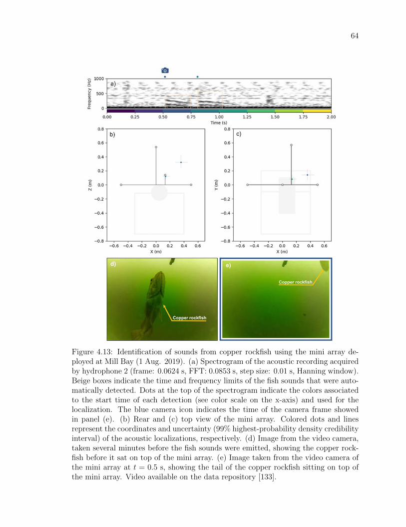
64

Figure 4.13: Identification of sounds from copper rockfish using the mini array de-ployed at Mill Bay (1 Aug. 2019). (a) Spectrogram of the acoustic recording acquiredby hydrophone 2 (frame: 0.0624 s, FFT: 0.0853 s, step size: 0.01 s, Hanning window).Beige boxes indicate the time and frequency limits of the fish sounds that were auto-matically detected. Dots at the top of the spectrogram indicate the colors associatedto the start time of each detection (see color scale on the x-axis) and used for thelocalization. The blue camera icon indicates the time of the camera frame showedin panel (e). (b) Rear and (c) top view of the mini array. Colored dots and linesrepresent the coordinates and uncertainty (99% highest-probability density credibilityinterval) of the acoustic localizations, respectively. (d) Image from the video camera,taken several minutes before the fish sounds were emitted, showing the copper rock-fish before it sat on top of the mini array. (e) Image taken from the video camera ofthe mini array at t = 0.5 s, showing the tail of the copper rockfish sitting on top ofthe mini array. Video available on the data repository [133].

65

Figure 4.14: Identification of sounds from copper rockfish using the mobile arraydeployed at Hornby Island (21 Sep. 2019). (a) Spectrogram of the acoustic recordingacquired by hydrophone 2 (frame: 0.0624 s, FFT: 0.0853 s, step size: 0.01 s, Hanningwindow). Beige boxes indicate the time and frequency limits of the fish sounds thatwere automatically detected. Dots at the top of the spectrogram indicate the colorsassociated to the start time of each detection (see color scale on the x-axis) andused for the localization. The yellow camera icon indicates the time of the cameraframe showed in panel (d). (b) Rear and (c) top view of the mobile array. Coloreddots and lines represent the coordinates and uncertainty (99% highest-probabilitydensity credibility interval) of the acoustic localizations, respectively. (d) Image fromthe underwater drone’s video camera and taken at t = 11.9 s, showing two copperrockfish at the front of the mobile array. Video available on the data repository [133].

66

Figure 4.15: Localization of unknown fish sounds using the mobile array deployed atHornby Island (18 Sep. 2019). (a) Spectrogram of the acoustic recording acquiredby hydrophone 2 (frame: 0.0624 s, FFT: 0.0853 s, step size: 0.01 s, Hanning win-dow). Beige boxes indicate the time and frequency limits of the fish sounds thatwere automatically detected. Dots at the top of the spectrogram indicate the colorsassociated to the start time of each detection (see color scale on the x-axis) and usedfor the localization. The green camera icon indicates the time of the camera frameshowed in panel (d). (b) Rear and (c) top view of the mobile array. Colored dotsand lines represent the coordinates and uncertainty (99% highest-probability densitycredibility interval) of the acoustic localizations, respectively. (d) Image from theunderwater drone’s video camera taken at t = 5.9 s, showing a blackeye goby and acopper rockfish in front of the mobile array. Video available on the data repository[133].

67

Figure 4.16: Localization of unknown fish sounds using the mobile array deployed atHornby Island (16 Sep. 2019). (a) Spectrogram of the acoustic recording acquired byhydrophone 2 (frame: 0.0624 s, FFT: 0.0853 s, step size: 0.01 s, Hanning window).Beige boxes indicate the time and frequency limits of the fish sounds that were auto-matically detected. Dots at the top of the spectrogram indicate the colors associatedto the start time of each detection (see color scale on the x-axis) and used for thelocalization. The turquoise camera icon indicates the time of the camera frame shownin (d). (b) Rear and (c) top view of the mobile array. Colored dots and lines representthe coordinates and uncertainty (99% highest-probability density credibility interval)of the acoustic localizations, respectively. (d) Image from the underwater drone’svideo camera taken at t = 3.8 s, showing a blackeye goby in front of the mobile array,defending its territory. Video available on the data repository [133].

68

(using the hydrophone closest to the sound source). The localizations from other

arrays were not precise enough to accurately estimate source level.

Table 4.2: Characteristics of the fish sounds identified. Duration, pulse frequency,pulse rate, and source level are reported by their mean ± the standard deviation.Asterisks (∗) indicate measurements for which there were not enough samples of fishsounds (n) to estimate the standard deviation.

Species Soundtype

Dur.(ms)

Pulse freq.(Hz)

Pulse rate(ms)

Source level(dB re 1µPa)

n

Lingcod Grunt 170∗ 301 ± 32 84.5 ± 10.5 115.4∗ 2Lingcod Pulse 19± 4 318 ± 13 N/A 113.0 ± 3.5 6Quillbackrockfish

Pulse 9 ± 1 387 ± 77 N/A 113.5 ± 2.0 13

Copperrockfish

Pulse 23± 2 163 ± 2 N/A - 5

4.5 Discussion

Results show that all three audio/video arrays can successfully identify fish sounds in

the wild. Field tests using a controlled sound source for each platform ground-truthed

the accuracy of the localization results and confirmed that the instrumentation and

analysis process are working correctly.

The large array provides the most accurate acoustic localizations and, with its

two video cameras, has the largest field of view. Note however, that localization

uncertainties are not represented similarly for all platforms. For the large array,

uncertainties are represented using one standard deviation while they are represented

by the 99% highest-probability density credibility interval for the mini and mobile

arrays. Hydrophone placement for this array was optimized using simulated annealing

to minimize localization uncertainties. This optimization resulted in a hydrophone

geometry that was different than the one used by Mouy et al. [76] to localize fish

sounds off Cape Cod. Using this hydrophone configuration increased by a factor of

about seven the spatial localization capacity of the array used in [76] (for the same

array volume) and allowed fish to be localized accurately (i.e., localization uncertainty

< 50 cm) at up to 3 m from the center of the array (Figure 4.5). The mini and mobile

arrays have a much smaller footprints and most of the sound sources to localize

69

are outside the array. Consequently, small errors in the measurement of the time-

difference of arrival lead to large errors in the localization results. Nevertheless, these

two arrays are capable of determining the bearing and elevation of the sound source,

which in many cases, is enough to confirm that the sounds recorded are emitted by the

fish in front of the camera (e.g., Figure 4.14). In some circumstances, when several

fish are located along the same bearing angle from the mini or mobile arrays, the large

localization uncertainties in range cannot identify with certainty the fish producing

the sound (e.g., Figure 4.15). This is typically not an issue if the fish are from the

same species.

While attempting to identify fish sounds in the wild using a single hydrophone

and a single camera is relatively inexpensive and logistically easy, our study shows

the importance of having several hydrophones (or directional sensors) for performing

acoustic localization. Inferring which individual fish produces the sounds, based only

on visual observations from video footage, is prone to errors and can lead to assigning

sounds to the wrong fish species. The case presented in Figure 4.8 is a good example

of this, where four fish are interacting together and for which the identification of the

individual fish emitting the sounds, only based on the video data, could be ambiguous.

Based on behavior only (i.e., without the acoustic localization), the emitted sounds

could have been either interpreted as a territorial display from the lingcod, or as a

reaction/defense display from the quillback rockfish. Another example illustrating

the usefulness of the acoustic localization is the recording with the blackeye goby

in Figure 4.16. Given, the clear territorial display of the blackeye goby observed

in the video, and the high signal-to-noise ratio of the fish sounds received by the

hydrophones, it would have seemed relatively evident to assign the fish sounds to this

individual. Performing the acoustic localization proved that this was not the case. It

is therefore critical to perform acoustic localization when cataloging fish sounds in a

natural setting.

In 2005, Rountree et al. [9] had already identified the need to combine passive

acoustic localization and underwater video to identify fish sounds in the wild. Our

work provides three different hardware and software solutions that attempt to fill this

research gap and help make passive acoustics a viable technique to monitor fish. Each

of the audio/video platforms that we developed have different constraints, strengths

and weaknesses. Given their different sizes, all arrays cannot be used in every habitat.

The large array requires a relatively flat bottom (at least a 4 m2 surface) and a water

depth of at least 6 m. The mini array can be deployed in more complex habitats with

70

rougher terrain and steeper slopes, and in shallower water (minimum of 3 m depth).

The mobile array can cover most types of habitat, from rough to flat sea bottom, from

very shallow (2 m) to deep (100 m) water depths, and can explore small crevasses

where fish can hide in. It can, however, not be used in areas with strong currents due

to reduced maneuverability. With proper ballast, the large and mini arrays are less

affected by currents. From a logistics perspective, the large array is the most complex

to deploy and recover. It requires at least two divers, two to three people at the surface

and a medium-sized motor boat. The mini array can be deployed with two divers and

one person at the surface. If deployed near shore, the mini array can be carried by

divers and no boat is needed. If deployed farther out, it can be deployed with a smaller

boat than for the large array. The mobile array is the easiest platform to deploy. It

only requires a single person piloting the underwater drone. It can be deployed from

shore or a dock, on a small boat, or from larger motor vessels. When deployed from

larger vessels, noise contamination from the engine and propellers must to be taken

into account, and all onboard machinery should be turned off when possible. Cost

wise, the large array uses six hydrophones and high-quality multichannel acoustic

recorder, which makes it the most expensive platform (∼ $40, 000 USD). The mini and

mobile arrays are less costly (∼ $8, 000 and $11, 000 USD, respectively). In terms of

the sampling, both the large and the mini arrays are static platforms that are deployed

over several weeks at a time. This long-term duration allows non-intrusive observation

and measurement of fish sounds related to a variety of behaviors. The short home-

range of some fish species [134], and the static nature of the large and mini arrays,

mean these platforms may only sample sounds from a small set of individuals. If this

is an issue, carrying out short deployments at different locations may be preferable

to performing a series of deployments at the same location. The mobile array can

sample several individuals over a larger spatial area but can only record for a few

hours. The mobile array is more intrusive than the two other arrays which tends to

more often elicit aggressive behaviors. Consequently, the mobile array may sample a

more restricted set of acoustic behaviors. As demonstrated in section 4.4, all arrays

can successfully attribute sounds to individual fish and therefore measure the temporal

and frequency characteristics of sound emitted by specific fish species. The large array

provides the most accurate localization and is consequently the preferred platform for

estimating source levels. Apart from infrequent cases, where the fish sits inside the

array (e.g., Figure 4.13), the localization from the mini and mobile arrays is typically

not accurate enough in range to allow accurate estimation of source levels. Figure

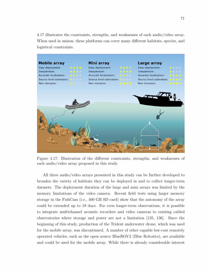
71

4.17 illustrates the constraints, strengths, and weaknesses of each audio/video array.

When used in unison, these platforms can cover many different habitats, species, and

logistical constraints.

Figure 4.17: Illustration of the different constraints, strengths, and weaknesses ofeach audio/video array proposed in this study

All three audio/video arrays presented in this study can be further developed to

broaden the variety of habitats they can be deployed in and to collect longer-term

datasets. The deployment duration of the large and mini arrays was limited by the

memory limitations of the video camera. Recent field tests using larger memory

storage in the FishCam (i.e., 400 GB SD card) show that the autonomy of the array

could be extended up to 19 days. For even longer-term observations, it is possible

to integrate multichannel acoustic recorders and video cameras to existing cabled

observatories where storage and power are not a limitation [135, 136]. Since the

beginning of this study, production of the Trident underwater drone, which was used

for the mobile array, was discontinued. A number of other capable low-cost remotely

operated vehicles, such as the open source BlueROV2 (Blue Robotics), are available

and could be used for the mobile array. While there is already considerable interest

72

in using passive acoustics for monitoring fish in coastal areas, there is also a growing

interest in exploring sounds produced by fish in deeper habitats [36, 137]. Due to

the low light conditions in the deep ocean, the design of our arrays would need to be

modified to sample in such environments. External LED lights could be added to the

FishCam on the array and could be controlled via its onboard single board computer

[84]. Alternatively, low-light cameras could be used [138].

Lingcod have not previously been documented to produce sound. Kelp greenling

(Hexagrammos decagrammus), which belong to the same family as lingcod (Hexa-

grammidae) and also do not have a swim bladder, have been reported to have mus-

cles possibly responsible for sound production [139], but their sounds have not been

recorded. A number of rockfish species have been reported to have sonic muscles

[139] and some have been documented to produce sounds [26, 78, 140]. Sounds from

quillback and copper rockfish have not been described in the peer-reviewed litera-

ture. However, a M.Sc. thesis from 2005 does provide some sound measurements

from these two species in captivity [140]. The source levels we measured (i.e. 113 dB

re 1 µPa) are consistent with the source levels measured for other species of rockfish

(i.e., 103–113 dB re 1 µPa [78]). Note that the sound measurements presented in

this study aim at illustrating the type of information that can be measured with the

audio/video arrays. A comprehensive description of the variability of the sounds from

each species based on the analysis of the entire dataset we collected will be the object

of a future study.

The source levels and temporal and spectral measurements of fish sounds are

key to monitor fish using passive acoustics. They are required to estimate how far

fish sounds can be detected and to investigate if fish species can be discriminated

acoustically. We show that such information can be reliably measured in situ in a

variety of habitats. We trust the open-source design we propose will help researchers

catalog and characterize fish sounds in other parts of the world.

4.6 Summary

Cataloging fish sounds in the wild is important for making passive acoustics a viable

tool for monitoring fish. Compared to lab studies, identifying fish sounds in the field

allows to record and characterize sounds from fish under a larger variety of behaviors.

However, it requires specialized equipment that can acoustically localize and visually

record fish in different habitats. In this study, we designed and tested three portable

73

audio/video platforms capable of identifying species-specific fish sounds in the wild:

a large array, a mini array, and a mobile array. The large and mini arrays are static

autonomous platforms than can be deployed on the seafloor and record audio and

video for up to two weeks. They use multichannel acoustic recorders (AMARs and

SoundTrap) and low-cost FishCam video recorders mounted on PVC frames. The

mobile array also uses a multichannel acoustic recorder (SoundTrap), but mounted

on an underwater drone with built-in video, which allows remote control and real-time

positioning in response to observed fish presence. Fish sounds were localized in three-

dimensions for all arrays and matched to the fish positions in the video data. The

hydrophone configuration of the large array was defined using a simulated annealing

optimization process which allowed this platform to have the most accurate acoustic

localization (i.e., uncertainties < 50 cm for fish located up to 3 m from the center

of the array). The mini and mobile arrays were able to resolve well the bearing and

elevation angles of the fish, but were less accurate at resolving the range. The large

array is the most expensive and, with its larger footprint, is well adapted to identify

fish sounds in relatively flat habitats. The mini array is the least expensive, easy to

deploy, and well adapted to rough/uneven seafloor. The mobile array can only record

for a few hours but is well suited for identifying sounds from fish between boulders

and in crevasses.

We deployed these three platform at four locations off the east coast of Vancouver

Island, British Columbia, Canada, and collected a total of 1214 hours of audio/video

data. From the analysis of a subset of these data, we identified, for the first time,

sounds from quillback rockfish (Sebastes maliger), copper rockfish (Sebastes caur-

inus), and lingcod (Ophiodon elongatus). In addition to measuring temporal and

spectral characteristics (i.e., pulse frequency, pulse repetition rate, and duration) of

sounds for each species, we estimated mean source levels for lingcod and quillback

rockfish sounds (115.4 and 113.5 dB re 1 µPa, respectively). We also show that iden-

tifying fish sounds in the wild without performing acoustic localization (i.e., with a

single omnidirectional hydrophone and camera) could lead to assigning sounds to the

wrong fish species.

4.7 Acknowledgments

Data collection in the field was made possible thanks to all the volunteers from the

Juanes Lab at the University of Victoria, Dr. Heloise Frouin-Mouy (NOAA), Dr. Dana

74

Haggarty (DFO), Dr. Sarah Dudas (DFO), and Scott Trivers. We would like to thank

James Pilkington (DFO) for providing the acoustic projector, and Marie Taureau for

producing the illustration in Figure 4.17. Thanks to Philippe Frouin for helping with

the design of the PVC frame for the large array. National Geographic and OpenROV

provided the Trident underwater drone through the Science Exploration Education

(S.E.E.) Initiative. All SCUBA divers involved in the deployment and recovery op-

erations were scientific divers certified by the Canadian Association for Underwater

Science (CAUS). This research is supported by the Natural Sciences and Engineer-

ing Research Council (NSERC) Canadian Healthy Oceans Network (CHONe) and its

partners: DFO and INREST (representing the Port of Sept-Iles and City of Sept-Iles),

JASCO Applied Sciences, and NSERC. X.M was also funded by an NSERC Postgrad-

uate Scholarship and a Mitacs Accelerate Fellowship. Field expenses and equipment

costs were funded by an NSERC Discovery grant, the Liber Ero Foundation, and

CFI/BCKDF funding.

75

Chapter 5

Automatic detection and

classification of fish sounds in

British Columbia

For this chapter, I designed and implemented all the analysis and processing scripts of

this study in Python, and created and documented the supporting open-source pack-

ages ecosound and FishSound Finder. Dr. Stephanie Archer made the majority of the

manual annotations from the Northumberland Channel Rockfish Conservation Area,

Emie Woodburn and Courtney Evans manually annotated fish sounds from Hornby

Island and Mill Bay, and I annotated fish sounds from the Delta node. Dr. Dana

Haggarty and Dr. Sarah Dudas collected the data from the Northumberland Chan-

nel Rockfish Conservation Area and I collected the data in the field at Mill bay and

Hornby Island. I wrote the paper with editorial assistance from Dr. Francis Juanes

and Dr. Stan Dosso.

5.1 Abstract

Many species of fish around the world have been reported to be soniferous. The

types of sounds fish produce vary among species and regions but consist typically of

low-frequency (< 1 kHz) pulses and amplitude-modulated grunts. These sounds can

potentially be used to monitor fish non-intrusively and could complement other more

traditional monitoring techniques. However, the significant time required for human

analysts to manually label fish sounds in acoustic recordings does not yet allow passive

76

acoustics to be used as a viable tool for monitoring fish. In this paper, we propose

an approach to automatically detect fish sounds in acoustic recordings from British

Columbia, Canada. First, acoustic transients are detected based on a measure of local

variance on the spectrogram. Second, each detected transient is represented by a set

of 45 features characterizing the sound distribution in time and frequency domain.

Third, extracted features are presented to a binary classifier to label the sound as

“fish” or “noise”. We tested 5 different classification algorithms (classification and

regression trees, gradient-boosted decision trees, random forest, linear discriminant

analysis, and logistic regression) and evaluated their performance on a dataset of

more than 96,000 manually-annotated fish and noise sounds from 5 different locations

off Vancouver Island and collected over all seasons of the year. The random forest

classifier with 50 trees performed best with an F score of 0.84 (Precision = 0.82,

Recall = 0.86). We show that the proposed approach can efficiently analyze long-

term datasets and make passive acoustics viable for fish monitoring. We provide an

open-source implementation of the fish detector along with detailed documentation.

5.2 Introduction

Over 800 species of fish worldwide are known to be soniferous [8, 9]. Fishes can pro-

duce sound incidentally while feeding or swimming (e.g., [12, 141]) or intentionally for

communication purposes [13, 14]. For example, the temporal and spectral character-

istics of fish sounds can convey information about male status and spawning readiness

to females [15], or about male body condition [16]. It has been speculated that some

species of fish may also emit sound to orient themselves in the environment (i.e., by

echolocation [17]). As is the case for marine mammal vocalizations, fish sounds can

typically be associated with a specific species and sometimes to specific behaviors [14,

18]. Several populations of the same species can have different acoustic dialects [19].

Consequently, it may be possible to use the characteristics of recorded fish sounds to

identify which species of fish are present in an environment, to infer their behavior,

and in some cases potentially identify and track a specific population [20]. Among

the approximately 400 known marine fish species frequenting the waters off British

Columbia, Canada, only 22 have been reported to be soniferous to date [10]. It is

believed that many more species produce sounds, but their repertoires have not yet

been identified. Several ongoing efforts aim to identify and characterize sounds from

more fish species in British Columbia [25], but many fish sounds still remain unknown

77

Figure 5.1: Spectrogram of unknown fish knock and grunt sounds recorded off HornbyIsland, British Columbia (1.95 Hz frequency resolution, 0.128 s time window, 0.012s time step, Hamming window). Knocks are the short pulses and grunts the longersounds with an harmonic structure.

(e.g., Figure 5.1).

Passive acoustic monitoring (PAM) of fish cannot only provide presence/absence

information, but in some cases it can also be used to estimate the relative abundance

of fish in an environment. By performing a simultaneous trawl and passive acoustic

survey, Gannon and Gannon [56] found that temporal and spatial trends in densities

of juvenile Atlantic croaker (Micropogonias undulatus) in the Neuse River estuary

in North Carolina could be identified by measuring characteristics of their sounds in

acoustic recordings (i.e., peak frequency, received levels). Similarly, Rowell et al. [57]

performed passive acoustic surveys along with diver-based underwater visual censuses

at several fish spawning sites in Puerto Rico and demonstrated that passive acoustics

could predict changes in red hind (Epinephelus guttatus) density and habitat use at a

higher temporal resolution than previously possible with traditional methods. More

recently, Rowell et al. [58] measured sound levels produced by spawning Gulf corv-

ina (Cynoscion othonopterus) with simultaneous density measurements from active

acoustic surveys in the Colorado River Delta, Mexico, and found that the recorded

levels were linearly related to fish density during the peak spawning period. While

passive acoustics shows great promise for monitoring fish populations, it is still largely

limited by knowledge gaps about the vocal repertoire of many fish species.

The manual detection of fish sounds in passive acoustic recordings is typically

performed aurally and by visually inspecting spectrograms. This is time-consuming

and laborious task, with potential biases which depend on the experience and the

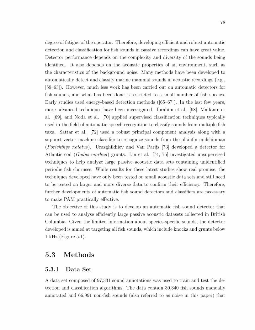
78

degree of fatigue of the operator. Therefore, developing efficient and robust automatic

detection and classification for fish sounds in passive recordings can have great value.

Detector performance depends on the complexity and diversity of the sounds being

identified. It also depends on the acoustic properties of an environment, such as

the characteristics of the background noise. Many methods have been developed to

automatically detect and classify marine mammal sounds in acoustic recordings (e.g.,

[59–63]). However, much less work has been carried out on automatic detectors for

fish sounds, and what has been done is restricted to a small number of fish species.

Early studies used energy-based detection methods ([65–67]). In the last few years,

more advanced techniques have been investigated. Ibrahim et al. [68], Malfante et

al. [69], and Noda et al. [70] applied supervised classification techniques typically

used in the field of automatic speech recognition to classify sounds from multiple fish

taxa. Sattar et al. [72] used a robust principal component analysis along with a

support vector machine classifier to recognize sounds from the plainfin midshipman

(Porichthys notatus). Urazghildiiev and Van Parijs [73] developed a detector for

Atlantic cod (Gadus morhua) grunts. Lin et al. [74, 75] investigated unsupervised

techniques to help analyze large passive acoustic data sets containing unidentified

periodic fish choruses. While results for these latest studies show real promise, the

techniques developed have only been tested on small acoustic data sets and still need

to be tested on larger and more diverse data to confirm their efficiency. Therefore,

further developments of automatic fish sound detectors and classifiers are necessary

to make PAM practically effective.

The objective of this study is to develop an automatic fish sound detector that

can be used to analyse efficiently large passive acoustic datasets collected in British

Columbia. Given the limited information about species-specific sounds, the detector

developed is aimed at targeting all fish sounds, which include knocks and grunts below

1 kHz (Figure 5.1).

5.3 Methods

5.3.1 Data Set

A data set composed of 97,331 sound annotations was used to train and test the de-

tection and classification algorithms. The data contain 30,340 fish sounds manually

annotated and 66,991 non-fish sounds (also referred to as noise in this paper) that

79

Table 5.1: Fish and noise annotations used to develop the fish sound classifier.

Location Acousticrecorder

Deploymentdate

Fishannot.

Noiseannot.

Totalannot.

Mill Bay AMAR Aug. 2019 3,699 24,330 28,029Hornby Isl. AMAR Sept. 2019 18,195 105 18,300Delta node AMAR Sept. 2014 831 0 831NC-RCA in SoundTrap Oct. 2018 6,677 8,434 15,111NC-RCA in SoundTrap Jan. 2019 0 8,036 8,036NC-RCA in SoundTrap Apr. 2019 0 6,742 6,742NC-RCA in SoundTrap Aug. 2019 0 2,353 2,353NC-RCA out SoundTrap Oct. 2018 938 1,844 2,782NC-RCA out SoundTrap Dec. 2018 0 5,047 5,047NC-RCA out SoundTrap Apr. 2019 0 10,100 10,100

Total: 30,340 66,991 97,331

were semi-automatically selected (Table 5.1). The fish sound annotations were per-

formed by five different analysts using the software Raven v1.6 (Cornell University,

Ithaka, NY) and PAMlab v8.4.2 (JASCO Applied Sciences, Dartmouth, NS). The

annotation process consisted of manually drawing time-frequency boxes around each

fish sound identified on the spectrogram (Figure 5.2a). To capture a spread of fish

sounds characteristics, noise conditions, and recording platforms, annotations were

performed from recordings collected at five different locations off Vancouver Island,

British Columbia (Mill Bay, Hornby Island, Ocean Network Canada’s Delta node in

the Fraser River delta, and inside and outside the Northumberland Channel Rockfish

Conservation Area - RCA), on a total of ten different deployments, and from three

different recording devices (Table 5.1, Figure 5.3).

Noise annotations were performed semi-automatically. First, sections of audio

recordings not containing any fish sounds were identified by an analyst. Then, the

detector (Section 5.3.2) was run on the selected recordings to automatically define the

time and frequency boundaries of all acoustic transients (Figure 5.2b). Recordings

used to create this noise data sets were chosen so it would include a large variety of

sounds such as noise from vessels, moorings, surface waves, and invertebrates (Table

5.1).

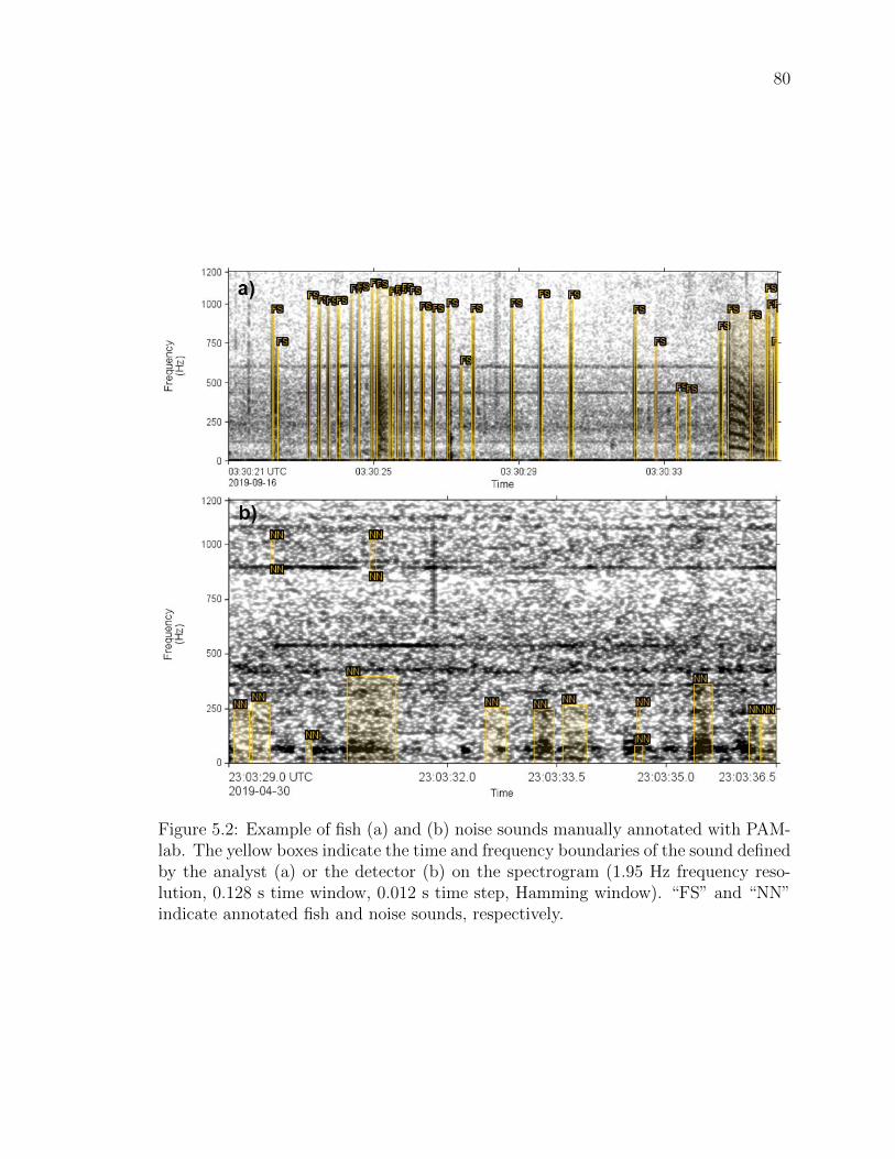
80

Figure 5.2: Example of fish (a) and (b) noise sounds manually annotated with PAM-lab. The yellow boxes indicate the time and frequency boundaries of the sound definedby the analyst (a) or the detector (b) on the spectrogram (1.95 Hz frequency reso-lution, 0.128 s time window, 0.012 s time step, Hamming window). “FS” and “NN”indicate annotated fish and noise sounds, respectively.

81

Figure 5.3: Map of the sampling locations. Black dots indicate the location of theacoustic recorders that were used to create the manually annotated fish and noisesound data sets. NC-RCA In and NC-RCA Out indicate recorders deployed insideand outside the Northumberland Channel Rockfish Conservation Area, respectively.

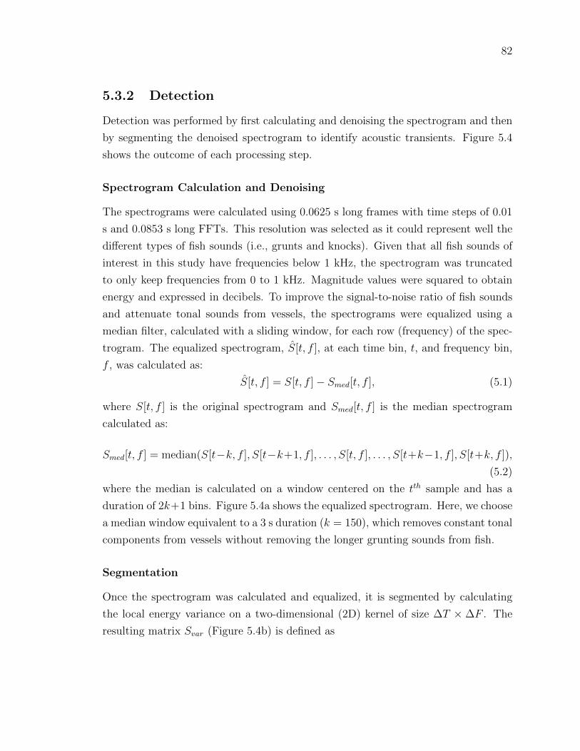
82

5.3.2 Detection

Detection was performed by first calculating and denoising the spectrogram and then

by segmenting the denoised spectrogram to identify acoustic transients. Figure 5.4

shows the outcome of each processing step.

Spectrogram Calculation and Denoising

The spectrograms were calculated using 0.0625 s long frames with time steps of 0.01

s and 0.0853 s long FFTs. This resolution was selected as it could represent well the

different types of fish sounds (i.e., grunts and knocks). Given that all fish sounds of

interest in this study have frequencies below 1 kHz, the spectrogram was truncated

to only keep frequencies from 0 to 1 kHz. Magnitude values were squared to obtain

energy and expressed in decibels. To improve the signal-to-noise ratio of fish sounds

and attenuate tonal sounds from vessels, the spectrograms were equalized using a

median filter, calculated with a sliding window, for each row (frequency) of the spec-

trogram. The equalized spectrogram, S[t, f ], at each time bin, t, and frequency bin,

f , was calculated as:

S[t, f ] = S[t, f ] − Smed[t, f ], (5.1)

where S[t, f ] is the original spectrogram and Smed[t, f ] is the median spectrogram

calculated as:

Smed[t, f ] = median(S[t−k, f ], S[t−k+1, f ], . . . , S[t, f ], . . . , S[t+k−1, f ], S[t+k, f ]),

(5.2)

where the median is calculated on a window centered on the tth sample and has a

duration of 2k+1 bins. Figure 5.4a shows the equalized spectrogram. Here, we choose

a median window equivalent to a 3 s duration (k = 150), which removes constant tonal

components from vessels without removing the longer grunting sounds from fish.

Segmentation

Once the spectrogram was calculated and equalized, it is segmented by calculating

the local energy variance on a two-dimensional (2D) kernel of size ∆T × ∆F . The

resulting matrix Svar (Figure 5.4b) is defined as

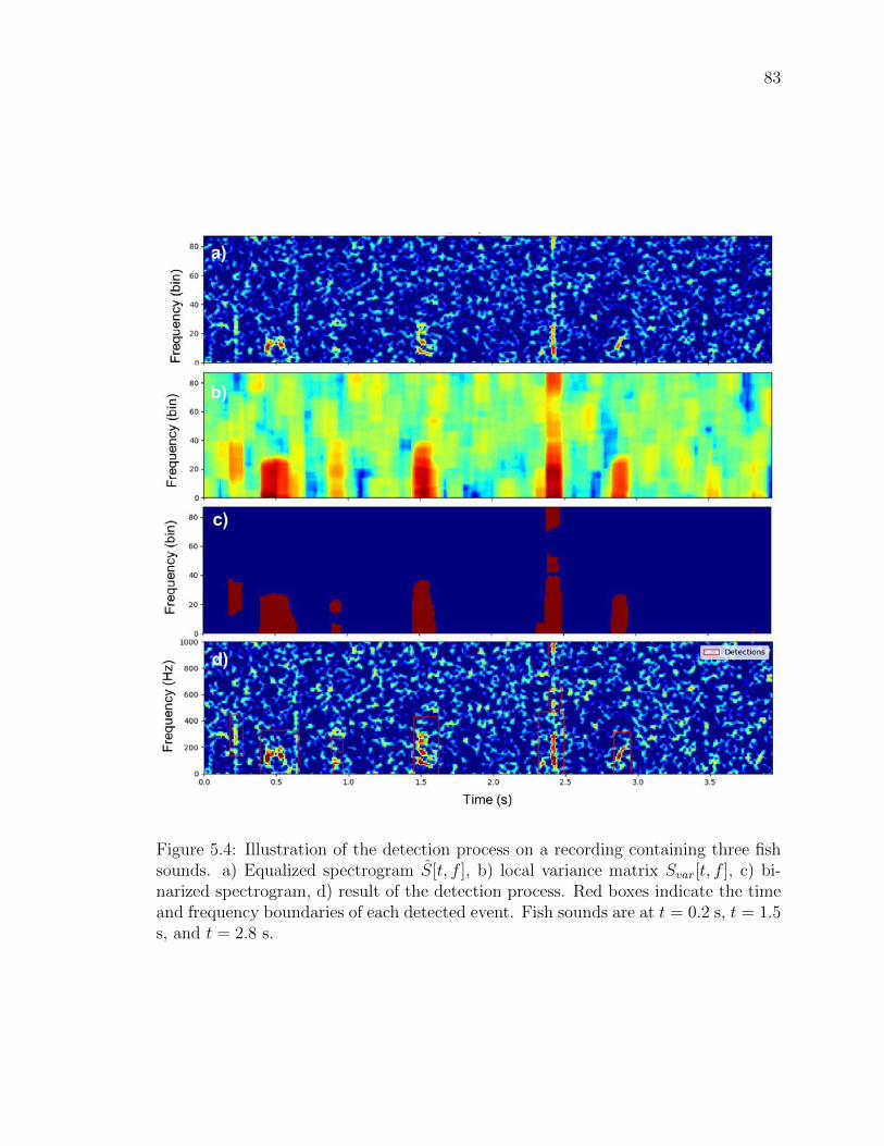
83

Figure 5.4: Illustration of the detection process on a recording containing three fishsounds. a) Equalized spectrogram S[t, f ], b) local variance matrix Svar[t, f ], c) bi-narized spectrogram, d) result of the detection process. Red boxes indicate the timeand frequency boundaries of each detected event. Fish sounds are at t = 0.2 s, t = 1.5s, and t = 2.8 s.

84

Svar[t, f ] =1

(∆T∆F ) − 1

t+∆T2∑

i=t−∆T2

f+∆F2∑

j=f−∆F2

|S[i, j] − µ|2, (5.3)

where µ is the mean over the 2D kernel:

µ =1

(∆T∆F )

t+∆T2∑

i=t−∆T2

f+∆F2∑

j=f−∆F2

S[i, j]. (5.4)

In this study, the number of time and frequency bins of the kernel are chosen to

be equivalent to 0.1 s and 300 Hz, respectively. Bins of the spectrogram with a

local variance less than 10 were set to zero and all the other bins were set to one

(Figure 5.4c). Bounding boxes of contiguous bins in the binarized spectrogram are

then defined using the outer border following algorithms described in [117]. These

bounding boxes define acoustic events of interest (red rectangles in Figure 5.4d) and

will be used in the next steps to determine whether they are fish sounds or not. To

speed up the classification process, all detected acoustic events shorter than 50 ms

or with a bandwidth smaller than 40 Hz were discarded. Figure 5.4 illustrates the

detection process on an acoustic recording containing three fish sounds.

5.3.3 Feature extraction

Each detection was represented by 45 features calculated from the (equalized) spectro-

gram, the spectral envelope, and the temporal envelope of the detected events (Figure

5.5, Table 3). The spectral envelope is the sum of the spectrogram energy values for

each frequency (Figure 5.5b). The temporal envelope is the sum of the spectrogram

energy values for each time step (Figure 5.5c). The spectral and temporal envelopes

were normalized to 1 and interpolated to have a resolution of 0.1 Hz and 1 ms, re-

spectively (red dots in Figure 5.5b,c). Spectrogram features were extracted based

on a time-frequency box that contained 95% of the energy of the initial detection

(white box in Figure 5.5a). Table 5.2 describes all features calculated to represent

the detections. Features were normalized before being used for classification, so all

have a mean of 0 and a variance of 1. These features were selected as they showed to

successfully represent animal sounds in a number of studies (e.g., [61, 142, 143]).

85

Figure 5.5: Extraction of features. a) Spectrogram of a fish detection. Red and blackcrosses denote the median and peak frequency of each time slice of the spectrogram,respectively. The white box indicates the 95% energy area over which the spectrogramfeatures were calculated. b) Spectral envelope of the detection. c) Temporal envelopeof the detection.

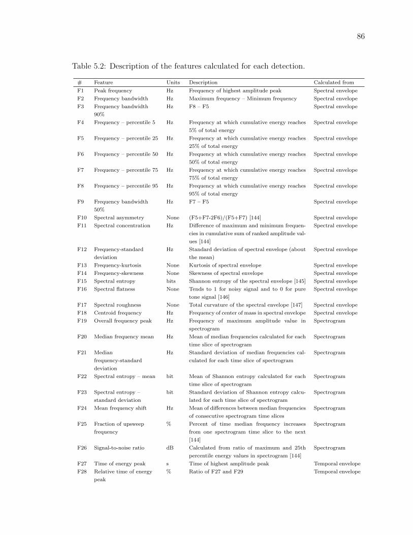
86

Table 5.2: Description of the features calculated for each detection.

# Feature Units Description Calculated from

F1 Peak frequency Hz Frequency of highest amplitude peak Spectral envelope

F2 Frequency bandwidth Hz Maximum frequency – Minimum frequency Spectral envelope

F3 Frequency bandwidth

90%

Hz F8 – F5 Spectral envelope

F4 Frequency – percentile 5 Hz Frequency at which cumulative energy reaches

5% of total energy

Spectral envelope


25% of total energy

Spectral envelope


50% of total energy

Spectral envelope


75% of total energy

Spectral envelope


95% of total energy

Spectral envelope

F9 Frequency bandwidth

50%

Hz F7 – F5 Spectral envelope

F10 Spectral asymmetry None (F5+F7-2F6)/(F5+F7) [144] Spectral envelope

F11 Spectral concentration Hz Difference of maximum and minimum frequen-

cies in cumulative sum of ranked amplitude val-

ues [144]

Spectral envelope

F12 Frequency-standard

deviation

Hz Standard deviation of spectral envelope (about

the mean)

Spectral envelope

F13 Frequency-kurtosis None Kurtosis of spectral envelope Spectral envelope

F14 Frequency-skewness None Skewness of spectral envelope Spectral envelope

F15 Spectral entropy bits Shannon entropy of the spectral envelope [145] Spectral envelope

F16 Spectral flatness None Tends to 1 for noisy signal and to 0 for pure

tone signal [146]

Spectral envelope

F17 Spectral roughness None Total curvature of the spectral envelope [147] Spectral envelope

F18 Centroid frequency Hz Frequency of center of mass in spectral envelope Spectral envelope

F19 Overall frequency peak Hz Frequency of maximum amplitude value in

spectrogram

Spectrogram

F20 Median frequency mean Hz Mean of median frequencies calculated for each

time slice of spectrogram

Spectrogram

F21 Median

frequency-standard

deviation

Hz Standard deviation of median frequencies cal-

culated for each time slice of spectrogram

Spectrogram

F22 Spectral entropy – mean bit Mean of Shannon entropy calculated for each

time slice of spectrogram

Spectrogram

F23 Spectral entropy –

standard deviation

bit Standard deviation of Shannon entropy calcu-

lated for each time slice of spectrogram

Spectrogram

F24 Mean frequency shift Hz Mean of differences between median frequencies

of consecutive spectrogram time slices

Spectrogram

F25 Fraction of upsweep

frequency

% Percent of time median frequency increases

from one spectrogram time slice to the next

[144]

Spectrogram

F26 Signal-to-noise ratio dB Calculated from ratio of maximum and 25th

percentile energy values in spectrogram [144]

Spectrogram

F27 Time of energy peak s Time of highest amplitude peak Temporal envelope

F28 Relative time of energy

peak

% Ratio of F27 and F29 Temporal envelope

87

Table 5.2 (continued): Description of the features calculated for each detection

# Feature Unit Description Calculated from

F29 Duration s Length of temporal envelope Temporal envelope

F30 Time-percentile 5 s Time at which cumulative energy reaches 5%

of total energy

Temporal envelope


of total energy

Temporal envelope


of total energy

Temporal envelope


of total energy

Temporal envelope

F34 Time-percentile 95 s Time at cumulative energy reaches 95% of total

energy

Temporal envelope

F35 Duration 50% s F33 – F31 Temporal envelope

F36 Duration 90% s F34 – F30 Temporal envelope

F37 Temporal asymmetry None (F31+F33-2F32)/(F31+F33) [144] Temporal envelope

F38 Temporal concentration s Difference of maximum and minimum times

in cumulative sum of ranked amplitude values

[144]

Temporal envelope

F39 Time – standard

deviation

s Standard deviation of temporal envelop. Temporal envelope

F40 Time-kurtosis None Kurtosis of temporal envelope Temporal envelope

F41 Time-skewness None Skewness of temporal envelope Temporal envelope

F42 Temporal entropy Bits Shannon entropy of a temporal envelope [145] Temporal envelope

F43 Temporal flatness None Flatness of temporal envelope. Tends towards

1 for noisy signal and towards 0 for pure tone

signal [146]

Temporal envelope

F44 Temporal roughness None Roughness of temporal envelope [147] Temporal envelope

F45 Temporal centroid s Time of center of mass in temporal envelope Temporal envelope

5.3.4 Classification

Features described in Section 5.3.3 were used to classify the detected events as either

“fish” or “noise”. Six different types of supervised classification algorithms were in-

vestigated: Classification and regression tree, gradient boosted decision trees, random

forest, linear discriminant analysis, logistic regression, and a dummy classifier used

as a baseline.

Classification and Regression Tree

A classification and regression tree (CART) is a supervised algorithm that can be

used for performing regression or classification tasks [148, 149]. In this study, we

used CART for classification. The principle of this algorithm is to predict the class of

an unknown sound by learning simple decision rules inferred from the data features.

During the training phase, the algorithm splits the training data (root) iteratively

88

into subgroups (nodes) based on one of the features. The choice of the rule and

feature at each split is based on a measure of entropy and is performed such that

the purity of the resulting nodes is maximized (i.e., maximizing the number of data

samples of the same class in each final node - also called leaf). The splits can be

performed until all leaves are pure (i.e., only containing data samples from the same

class), or until some conditions are met (e.g., until a minimum number of samples is

in a leaf). Once the set of rules are defined in the training phase, they can be used for

classifying an unknown data sample. The sample is run through the sets of conditions

of the tree and the label of the leaf the unknown sample ends up in, defines its class.

A probability of confidence is associated to the predicted class and is defined as the

fraction of samples of the same class in the leaf of the unknown sample. For this

study, splits of the CART were performed using the Gini impurity, and nodes were

expanded until all leaves contained a minimum of two data samples.

Gradient Boosted Decision Trees

Gradient boosted decision is a classification technique based on the concept of an

ensemble. It performs classification not using a single decision tree (e.g., CART), but

an ensemble(collection) of decision trees [150]. It starts by fitting an initial model

to the data. Then a second model is fit on a modified version of the original data

set that focuses on accurately predicting the cases where the first model performed

poorly. The combination of these two models is expected to be better than either

model alone. Then, this “boosting” process is repeated many times. Each successive

model attempts to correct for the shortcomings of the combined boosted ensemble of

all previous models. For this study, we used the XGBoost implementation of gradient

boosted decision trees with a maximum tree depth of 6 and 100 trees [151].

Random Forest

Random forest (RF) is also a classification technique based on the concept of an

ensemble. A random forest is a collection of decision trees [152], where each tree is

grown independently using binary partitioning of the data based on the value of one

feature at each split (or node). When features measured from a sample or, in our

case, a sound, are run through the random forest, each tree in the forest produces a

classification and the sound is classified as the class that the greatest number of trees

vote for. Randomness is injected into the tree-growing process in two ways: 1) each

89

tree in the forest is grown using a random subsample of the data in the training data

set and 2) the decision of which feature to use as a splitter at each node is based

on a random subsample of all features [152]. Each tree is grown to its maximal size.

Using an ensemble of trees with splitting features chosen from a subset of features at

each node means that all important features will eventually be used in the model. In

contrast, a single decision tree is limited to a subset of features (unless the number

of features is small or the tree is large) and can be unstable (small changes in the

data set can result in large changes in the model; [153]). The ensemble decision

approach has been shown to result in lower error rates than can be achieved using

single decision trees (e.g., [154]). In this study, we tested random forest models with

5 (RF5), 10 (RF10), 30 (RF30), and 50 (RF50) trees. For all these test models, the

random subset of features used for each splits was set to 6.

Linear Discriminant Analysis

A linear discriminant analysis (LDA) classifier consists of defining a linear decision

boundary generated by fitting class conditional densities to the data and using Bayes’

rule (Section 2.6.2 in [155]). It assumes that features for each class have a normal

distribution and all have the same variance. In this study, we fitted the model to

the data using singular value decomposition. This method is attractive given that it

returns a closed-form solution that is straightforward to compute and has no hyper-

parameters to tune. The LDA algorithm is well known and serves as a reference for

the other more advanced algorithms used in this work (i.e., gradient boosted trees,

and random forest).

Logistic Regression

Logistic regression (LR) is a linear model for binary classification. It is similar to

linear regression (which is not used for classification), but instead of fitting a line to

the data, fits a sigmoid (also called logistic) function that allows the best separation

of two classes [155]. In this study, the logistic function parameters were estimated

using the LBFGS algorithm using an L2 norm penalty [156]. As for the LDA, LR is

a well-known algorithm for binary classification (which is our case here: fish versus

noise) and serves as a reference for the other more advanced algorithms.

90

Figure 5.6: Description of the data used in the training and testing data sets. Labelson the x-axis indicate the class of the annotations (i.e., fish or noise) followed by theidentification of the deployment they were from (see Table 5.1).

Dummy classifier

Finally, we used a dummy classifier as a baseline for other classification methods. It

consisted of classifying all unknown data as being fish.

5.3.5 Experimental Design

Classification models were trained and tested by dividing the data set of annotated

sounds (Section 2.1.1) into two subsets. One was composed of 75% of the entire

data set and was used to train the classification models, tune their hyperparameters,

and identify which one performed best (blue bars in Figure 5.6). The other one,

representing 25% of the entire data set, was used to evaluate the performance of

the selected model. These two subsets were carefully defined so that they did not

share annotations made from the same hour of recording, had the two classes (fish

and noise) equally represented, and had a similar representation of all deployments

(Figure 5.6). Data used for testing the performance of the classification were never

used for training the models.

91

Figure 5.7: Illustration of the protocol used to train and evaluate the performance ofthe different classification models.

The different classification methods were evaluated on the training set using a

five-fold cross-validation strategy. Folds were defined by splitting the training into

5 subsets. As done previously for creating the training and test sets (Figure 5.1),

folds were defined so that they did not share annotations made from the same hour

of recording, had the two classes (fish and noise) equally represented, and had a sim-

ilar representation of all deployments. Each classification method was evaluated five

times by, in turn, using data from four folds for training the model and data from

the remaining fold for evaluating its performance. This cross-validation procedure

was repeated five times by shuffling the training data before redefining the folds.

Consequently, each classification algorithm was trained and evaluated 25 times. The

performance of each algorithm was represented by the mean and variance of its classi-

fication performance over the 25 cross-validations. At the end of the cross-validation

process, a total of 200 models were trained and evaluated (i.e., 8 algorithms × 25

cross-validations). The algorithm that performed best during the training phase was

retrained using the entire training set and was tested on the test data set. Figure 5.7

illustrates the training and testing procedure.

Given that the annotated data were imbalanced (i.e., many more noise annotations

than fish annotations, Table 5.1), two resampling methods were adopted before the

training of each model. First, the Tomek links method was used to under-sample

the majority class (here noise). It consists of identifying pairs of nearest neighbors

92

in a data set that have different classes and then removing the examples from these

pairs belonging to the majority class. This has the effect of reducing the number of

samples in the majority class, while making the decision boundary in the training

data set less noisy or ambiguous [157]. Second, the synthetic minority over-sampling

technique (SMOTE) was used to over-sample the minority class (here fish). It consists

of artificially creating new data points by selecting examples of the minority class that

are close in the feature space, drawing a line between them, and drawing a new data

point as a point in the feature space along that line [158]. Theses two methods were

used to obtain a balanced data set (i.e., equal number of fish and noise samples)

before training the classification models.

5.3.6 Performance

The decisions generated from the classifiers can be categorized as follows:

True positives (TP ): A signal of interest being correctly classified as such;

False positives (FP ): Noise classified as a signal of interest (i.e., a false alarm);

and

False negatives (FN): A signal of interest that is classified as noise (i.e., missed).

To calculate the numbers of TP s, FP s, and FNs, the manual annotations of

fish sounds, which are considered true results, were compared with the automated

classifications. To assess the performance of the detectors, precision (P ) and recall

(R) metrics were calculated based on the numbers (N) of TP s, FP s, and FNs, as:

P =NTP

NTP + NFP

, R =NTP

NTP + NFN

, (5.5)

where P measures exactness and R measures completeness. For instance, a P of 0.9

means that 90% of the detections classified as fish sounds were in fact fish sounds but

says nothing about whether all sounds in the data set were identified. An R of 0.8

means that 80% of all fish sounds in the data set were correctly classified, but says

nothing about how many classifications were wrong. Thus, a perfect classifier would

have P and R equal to 1. Neither P nor R alone can describe the performance of

a detector/classifier on a given data set; both metrics are required. The F score is

also used to quantify classifier performance. The F score measures the accuracy of

93

the detector and varies from 0 to 1, where an F score of 1 corresponds to a perfect

detector. It is defined as

Fβ = (1 + β2)PR

β2P + R, (5.6)

where β is the relative weight between the recall and precision. A β of 2 means

the recall has double the weight of the precision. Conversely, a β of 0.5 means the

recall has half the weight of the precision. In this work, it was considered that P and

R were equally important, so the unweighted F score was used (i.e., β = 1).

All classifiers used in this study provide classification results (i.e., “fish” or “noise”)

as well as a confidence of classification comprised between 0 and 1. The latter can

be used to adjust the sensitivity of a classifier. Accepting classification results with a

low confidence will lead to detecting more fish sounds (i.e., high recall), but will also

generate more false alarms (low precision). Conversely, only accepting classification

results with a high confidence will lead to detecting fewer fish sounds (low recall),

but will also result in fewer false alarms (high precision). Therefore, the precision,

recall, and F score were calculated separately for confidence values going from 0 to 1

in increments of 0.02.

5.3.7 Implementation

The fish sound detection and classification algorithms described in this paper were

implemented in Python 3.8 using the open source library ecosound [124]. Ecosound

is a python toolkit with several building blocks that help develop automatic detectors

and classifiers and deploy them at large scale (from single workstations to computer

clusters). It relies on the Python libraries pandas [125], NumPy [126], scikits-learn

[127], Dask [128], and xarray [129], and is compatible with annotations from the

bioacoustics software Raven (Cornell University, Ithaca, NY), and PAMlab (JASCO

Applied Sciences, Dartmouth, NS). The fish sound detector/classifier has been re-

leased as the standalone python package FishSound Finder [159]. Both ecosound and

FishSound Finder are released under the BSD-3-Clause License and can be installed

using the Python Package Index (pypi.org).

94

5.4 Results

Figure 5.8 and Table 5.3 show the performance results of the classification models

on the training data set via cross validation. The dummy classifier (baseline) had

a mean precision of 0.343, recall of 1.00, and F score of 0.498. The LDA classifier

performed the worst compared to the other algorithms, with a mean precision of

0.64, recall of 0.795, and F score of 0.70. The LR classifier also did not perform well,

with performance results close to those obtained with LDA. RF and gradient boosted

trees (XGBoost), which are the more-complex ensemble-based algorithms, performed

substantially better (i.e., with an F score increased by at least 5%) than LDA and

RF.

Increasing the number of trees in the RF classifier from 5 to 30 increased the F

score by approximately 5%. However, training RF models with more than 30 trees

did not substantially improve the performance. The RF classification model with 50

trees performed best, with a mean precision of 0.75, recall of 0.845, and F score of

0.792.

Most classifiers performed best when used with a confidence threshold between

0.5 and 0.6 (Figure 5.8). Performance of the RF classification model with 50 trees

calculated on the test data set was slightly higher than the one calculated by cross-

validation on the training data set, with a precision of 0.82, recall of 0.86, and F score

of 0.84 (Table 5.4). Noise samples were well classified on the test data set, with an

F score of 0.94.

Figure 5.8: Performance of the fish sound classifier on the training data set: a)Average precision and recall and (b) average F score calculated over all confidencethresholds for the eight (plus the dummy baseline) classification models tested.

95

Table 5.3: Performance of all the classification models on the training data set fora confidence threshold of 0.5 (mean ± standard deviation). RF5, RF10, RF30, andRF50 correspond to the RF models trained with 5, 10, 30, and 50 trees, respectively.

XGBoost CART RF5 RF10 RF30 RF50 LDA LR Dummy

Precision 0.70 ±0.13 0.68±0.12

0.72±0.11

0.73±0.11

0.75±0.11

0.75±0.11

0.64±0.17

0.64±0.15

0.34±0.13

Recall 0.83 ±0.05 0.04±0.71

0.83±0.04

0.83±0.04

0.84±0.04

0.84±0.04

0.79±0.08

0.79±0.08

1.00±0.00

F score 0.76 ±0.09 0.71±0.08

0.76±0.08

0.72±0.08

0.79±0.07

0.79±0.07

0.70±0.14

0.70±0.12

0.50±0.15

96

Table 5.4: Performance of the random forest model with 50 trees on the test data setfor a confidence threshold of 0.5. This model was trained using the entire trainingdata set.

Class Precision Recall F score # sounds

Fish 0.82 0.86 0.84 6758Noise 0.95 0.93 0.94 17666

5.5 Discussion and conclusion

The methods developed here for automatically detecting fish sounds show satisfactory

performance results on the dataset of manually annotated recordings. Emsemble-

based classifiers (RF and XGBoost) performed better than other more traditional

methods (LDA, LR). The F score we obtained with the RF classifier with 50 trees (F

score = 0.84) is comparable to the Sciaenidae sound detector described in [160] (F

score = 0.86), but lower than the generic fish detector in [69] (F score 0.9). Noda et

al. [70] obtained an F score of 0.98 in automatically classifying sounds from 128 fish

species. The latter study was based on a small dataset of sounds recorded in tanks

and did not include classification of noise (i.e., non-fish) recordings. Several other fish

sound detectors have been developed but focus on detecting periodic fish chorusing

events rather than individual fish sounds (e.g., [74, 161]). The calculated performance

of automatic detectors and classifiers dependents strongly on the datasets used to

both train and test the algorithms. Evaluating algorithms on small datasets (e.g.,

several hundred sounds collected over a few days), where noise conditions, fish species

present, and recording platforms do not change or are very stable and predictable,

can lead to high performance scores, which may not be representative of how these

algorithms would behave when applied to large continuous passive acoustic datasets.

The large dataset we use is comprised of more than 97,000 fish and noise sounds

collected over 5 different sites (some, like Delta Node and NC-RCA-In, located in

noisy vessel shipping routes), and spanning all seasons of the year, which provides

confidence that the detectors characterized in this paper would behave similarly on

long-term continuous datasets.

The methods developed here are target individual fish knocks and grunts which

97

are the most common sounds recorded in British Columbia (e.g., Figure 5.1). Longer

continuous sounds from chorusing fish found in British Columbia, such as plainfin

midshipman (Porichthys notatus) boat-whistles [162], would not be successfully de-

tected with the proposed approach. The methods developed in this study target fish

sounds in general without differentiating knocks from grunts. It may be useful to

retrain the classification models to recognize these two sound types separately. Ad-

ditionally, as more sounds from fish are identified, it would be useful to train the

classification model to recognize specific species. This may require using different ad-

vanced methods such as deep neural networks [163–165]. While we tested the detector

on a large dataset, we recognize that this only considered recordings off the east coast

of Vancouver Island. Testing the detector in other parts of British Columbia will be

part of future studies.

Based on the dataset collected at Hornby Island for this study, it takes approx-

imately 48 hours of continuous work (equivalent of six 8-hour working days) for a

human analyst to manually annotate one day (24 hours) of continuous recording.

In comparison, the RF based detector described here (RF50) processes one day of

continuous recording in approximately 4 hours and does not require human supervi-

sion. Using such automated algorithms for detecting and labeling fish sounds makes

passive acoustics a more viable tool to help fish monitoring and marine conservation.

Automatic detectors still require some level of manual analysis from human analysts

to validate the detection results. However, several manual analysis methodologies

[166] and software solutions [167, 168] can be employed to make this process more

efficient.

To illustrate the potential of the proposed algorithm, we ran it on 2.5 months of

acoustic data. Figure 5.9 shows the automatic detections from the RF50 detector

that was run on continuous data collected in the Northumberland Channel Rockfish

Conservation Area (see map in Figure 5.3) from April 10 to June 25, 2019. From

these detection results, it is possible to quickly identify periods with (Figure 5.9a)

and without (Figure 5.9c) fish sounds, which provides initial insights on the variation

of the number of fish sounds over the entire deployment. Just using Figure 5.9b it

is possible to observe three possible trends in the data: 1) The oblique patterns of

elevated detections suggest that occurrence of fish sounds may correlate with tide

cycles; 2) the number of fish sounds appears to increase gradually from April to June;

and 3) more fish sounds were detected during the night than during the day. While a

rigorous analysis is required to confirm these initial observations, this result illustrates

98

Figure 5.9: Automatic detection of fish sounds inside the Northumberland ChannelRCA from April to June 2019. a) Spectrogram of a 30 s recording from May 19with no fish sounds, b) heat map representation of the number of automatic fishdetections per hour, c) spectrogram of a 30 s recording from May 26 with more than60 fish sounds. Spectrogram resolution: 1.95 Hz frequency resolution, 0.128 s timewindow, 0.012 s time step, Hamming window.

99

how useful the automatic detector can be to quickly explore large datasets, formulate

hypotheses, and answer practical conservation questions.

It has been known for a long time that fish produce sounds. However, the use their

sounds in passive acoustic monitoring programs is still uncommon. One reason fish

sounds are underused in marine conservation is because the analysis tools developed

by engineers are rarely made accessible to other researchers in the marine conservation

field. The software implemented in this paper is released under an open source license

and is accompanied with a step by step tutorial showing how to use it [159]. Our

hope is that it will be used, further tested, and improved by other researchers in the

community.


This research was funded by Fisheries and Oceans Canada (DFO), the Liber Ero

Foundation, a Natural Sciences and Engineering Research Council (NSERC) Dis-

covery Grant, and the NSERC Canadian Healthy Oceans Network and its Partners:

DFO and INREST (representing the Port of Sept-Iles and City of Sept-Iles). X.M. was

also supported by a NSERC Postgraduate Scholarships-Doctoral scholarship, JASCO

Applied Sciences, and a MITACS Accelerate fellowship. Data from the Northum-

berland Channel RCA were provided by Dr. Dana Haggarty (DFO) and Dr. Sarah

Dudas (DFO). Data from the Delta Node were provided by Ocean Networks Canada.

Dr. Stephanie Archer (Louisiana Universities Marine Consortium), Dr. Philina En-

glish (DFO), Ms. Emie Woodburn (University of Victoria), and Ms. Courtney Evans

(University of Victoria) manually annotated fish sounds from the data collected at

Northumberland Channel RCA, Hornby Island and Mill Bay. Thanks to Ms. Karen

Scanlon (JASCO Applied Sciences) for an initial editorial review of this manuscript.

100

Chapter 6

Discussion and Perspectives

The overarching objective of this thesis was to make passive acoustics a more viable

and accessible tool to monitor fish in their natural habitat. The work specifically

consisted of developing and testing a set of methodologies to facilitate the identifica-

tion of sounds that fish produce in their natural environment and make the analysis

of large passive acoustic datasets more efficient. It involved the development of both

hardware and software solutions. On the hardware side, a low-cost autonomous un-

derwater camera capable of recording video for several weeks was developed. Three

easy-to-build audio/video array designs were also proposed to catalog fish sounds

in various habitats. On the software side, an open-source library was developed to

automatically detect fish sounds, optimize hydrophone placement, and perform 2D

acoustic localization. These solutions were tested in the field and enabled the de-

scription of sounds from fish that had not been reported to produce sound before.

Many of the audio/video methods developed in this thesis are based on ideas that

were proposed several decades ago by founding researchers of the fish bioacoustics

community [9]. For example, in 1968 Breder already use of acoustic localization to

study fish sounds using an apparatus called the audiogoniometer [169]. Sprague and

Luczkovich in 2004 [29], then Rountree and Juanes in 2010 [30] had used Remotely

Operated Vehicles (ROVs) to simultaneously record audio and video to study fish.

In 2015, Locascio and Burton [31] developed customized underwater audio and video

systems to verify sources of fish sounds in Florida. Many of these methods are the

foundation of what fish bioacoustics is today. However, due to the prohibitive costs,

logistical constraints, and technical challenges, the specialized equipment required is

not easy to use and accessible only to a small group of researchers. This thesis took

advantage of recent advances in technology to transform these conceptual ideas into

101

practical tools that are relatively inexpensive, easy to replicate, and accessible to the

research community and also potentially to interested citizen scientists. The recent

democratization of small single-board computers, such as the Rapsberry Pi, now al-

lows us to relatively easily build sophisticated and fully customizable instruments at

a low-cost, such as the FishCam described in Chapter 3 [170]. The recent advances of

small ROVs have also played an important role in this thesis. Unlike the large ROVs

used by Sprague and Luczkovich [29] and Rountree and Juanes [30], the underwater

drone used for the mobile audio/video array in Chapter 4 was inexpensive (< $3, 000

USD), easy to operate from a small boat or from shore, and quiet when not moving.

The Trident was one of the first reliable underwater drones to become available on the

market when this thesis started. Now, many more models and designs of underwater

drones exist and have a variety of specialized capabilities (e.g., robotic arm, built-in

echosounders). This will allow even further development and democratization of plat-

forms such as the mobile array proposed in Chapter 4. Advances in passive acoustic

recorder technology were also key in making two of the proposed audio/video arrays

relatively inexpensive and compact. We showed that performing acoustic localization

is highly recommended for identifying fish sounds in the wild. However this implies

the use of autonomous multichannel recorders with at least four channels, which are

typically more expensive than single-hydrophone systems. The four-channel Sound-

Trap recorder used for the mini and mobile arrays was introduced in recent years and

made acoustic localization possible at a reasonable cost and with a minimal fooprint.

New generations of low-cost (< $100 USD) open-source audio recorders such as the

AudioMoth [104] are currently revolutionizing passive acoustic monitoring on land,

and are expected to be adapted to the aquatic environment in the near future. This

will likely result in making audio/video platforms for identifying fish sounds even

more affordable and lightweight.

Fish have been known to produce sounds for a very long time, but their sounds

have arguably been under-studied compared to more charismatic marine fauna (e.g.,

whales), despite the value of passive acoustics for fisheries management. This dif-

ference can be attributed partially to the technology that was not always available

and affordable (as mentioned above), but also to the general lack of interest in this

topic. Thanks to founding researchers in the field, substantial efforts have been made

to educate funding agencies, research communities and the general public, which led

to a increase of interest in fish bioacoustics in the last decade [9, 171–173]. Another

reason that fish sounds have been under-studied, is the lack of accessibility and repro-

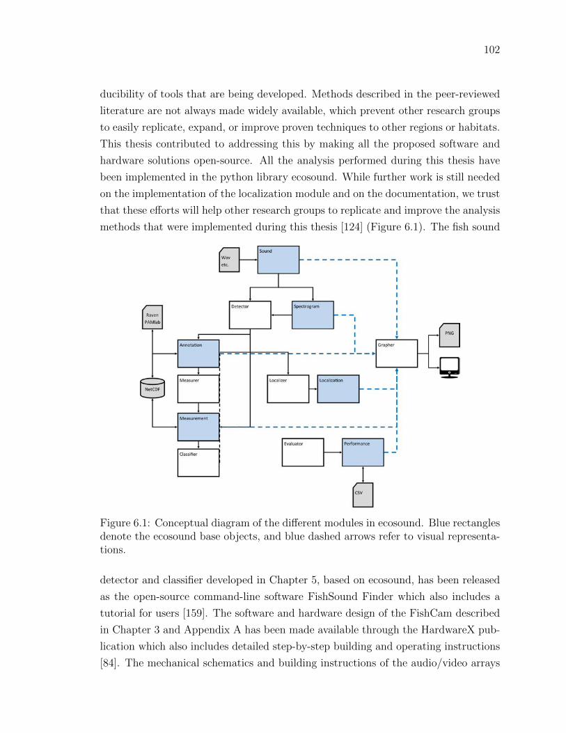
102

ducibility of tools that are being developed. Methods described in the peer-reviewed

literature are not always made widely available, which prevent other research groups

to easily replicate, expand, or improve proven techniques to other regions or habitats.

This thesis contributed to addressing this by making all the proposed software and

hardware solutions open-source. All the analysis performed during this thesis have

been implemented in the python library ecosound. While further work is still needed

on the implementation of the localization module and on the documentation, we trust

that these efforts will help other research groups to replicate and improve the analysis

methods that were implemented during this thesis [124] (Figure 6.1). The fish sound

Figure 6.1: Conceptual diagram of the different modules in ecosound. Blue rectanglesdenote the ecosound base objects, and blue dashed arrows refer to visual representa-tions.

detector and classifier developed in Chapter 5, based on ecosound, has been released

as the open-source command-line software FishSound Finder which also includes a

tutorial for users [159]. The software and hardware design of the FishCam described

in Chapter 3 and Appendix A has been made available through the HardwareX pub-

lication which also includes detailed step-by-step building and operating instructions

[84]. The mechanical schematics and building instructions of the audio/video arrays

103

and the acoustic localization scripts used in Chapter 4 have not been included in

this thesis but will be included as supplementary material when this chapter is sub-

mitted for publication. The FishSound Finder software is currently being tested by

organizations in Canada (DFO), United States (Louisiana Universities Marine Con-

sortium), and Norway (Norwegian Institute for Nature Research). The FishCam is

also currently being built and improved by several companies in British Columbia

(ASL Environmental Science Inc., Cascadia Seaweed).

Fish sounds are being recorded in many places along the coast of British Columbia

from Haida Gwaii to Southern Vancouver Island ([10, 81, 174], Lynn Lee pers. comm.,

Scott Veirs pers. comm.). This widespread interest shows the potential of passive

acoustics for monitoring fish in British Columbia. However, many of these sounds are

still not identified to specific species. This thesis has begun to address this knowledge

gap for the Strait of Georgia by identifying sounds from quillback rockfish, copper

rockfish, and lingcod. While several weeks of data have been collected with the au-

dio/video arrays, only a subset were analyzed due to time-contraints. The sounds

identified and described demonstrated the capabilities of the proposed arrays, but

cannot fully describe the extend of the acoustic repertoire of these species. The anal-

ysis of the entire dataset will be performed in future work. A key constraint in making

passive acoustic monitoring of fish successful and efficient in British Columbia will

be the ability to discriminate sounds from these different species using a single hy-

drophone without video cameras. Time and frequency characteristics of the sounds

identified in this thesis suggest that it may be possible to distinguish species based on

the pulse frequency and duration (Figure 6.2). It is, however, important to consider

Figure 6.2: Pulse frequency and duration of the single pulse sounds idendified inChapter 4.

that this preliminary observation is only made from a small set of fish sounds. Al-

104

though several fish species produce sounds that have distinct frequency and temporal

characteristics [82], fish sound properties can also fluctuate with behavior, water tem-

perature and fish size [77, 175, 176]. Therefore, it will be important to analyze the

entire dataset collected with the audio/video arrays to better describe the variability

of sounds for each species to determine the validity of this initial observation. It will

also be important to take into account other descriptors quantifying sound rhythm

[177] and temporal context [178]. If passive acoustic species discrimination is con-

firmed, then automatic detection and classifications methods described in Chapter 5

can be adapted to target specific species.

Data from the large audio/video can provide estimates of the source level of the

fish sounds. This information is key in designing passive acoustic monitoring pro-

grams as it helps to 1) define the distance over which fish sounds can be detected,

2) determine how many recorders are required for the area of interest, and 3) assess

if passive acoustic monitoring is suitable for an area, given its ambient noise condi-

tions. If we assume that fish sounds with a received level below the ambient noise

are not detectable (i.e. detection threshold of 0 dB), and that sound waves spread

spherically without absorption, then the maximum distance R at which fish sounds

can be detected is estimated as

R = 10SL−NL

20 , (6.1)

where SL is the source level, and NL is the noise level at the monitoring location.

Table 6.1 shows the estimated detection ranges at the Mill Bay and Hornby Island

locations where the large audio/video array was deployed (Figure 4.7, Table 4.1). The

calculation was performed using a source level value of 113 dB re 1µPa (as measured

in Table 4.2) and noise levels measured at the middle hydrophone of the large array

between 20 and 1000 Hz (i.e., the frequency band of fish sounds) using the software

PAMGuide [179]. Given that noise levels constantly fluctuate in time, the detection

range was calculated for the minimum (Lmin) and maximum (Lmax) noise levels, as

well as for the 5th, 50th, and 95th percentile levels (L5, L50, and L95, respectively).

Detection range values in Table 6.1 show that at Hornby Island, fish sounds can be

detected at up to 33 m under the quietest conditions (Lmin), but only up to 8 m for

half of the time (L50). At Mill Bay, the detection range is less than 11 m under the

quietest conditions and less than 2 m for half of the time. During the noisiest events

(Lmax), typically when a boat is passing close by, fish sounds are only detectable

105

Table 6.1: Estimated detection range (R) of fish sounds at Mill Bay and HorbnyIsland. Noise levels (NL) were computed in the 20-1000 Hz frequency band everyminute by averaging 120 1 s long Hann-windowed fast Fourier transforms overlappedby 0.5 s.

Mill Bay Horny IslandNL (dB re 1µPa) R (m) NL (dB re 1µPa) R (m)

Lmin 92.6 10.5 82.6 33.0L5 102.2 3.5 87.2 19.6L50 107.9 1.8 95.0 7.9L95 116.1 0.7 105.1 2.5Lmax 146.9 0.0 130.1 0.1

over a few centimeters for both locations. These results illustrate well how source

levels are needed to assess spatial coverage and define a monitoring plan. The Mill

Bay site is near a marina and is noisier than Hornby Island, which results in smaller

detection ranges. Consequently, developing a passive acoustic monitoring program

for fish would likely require deploying more acoustic recorders at Mill Bay than at

Hornby Island. Such analysis may also help define areas where passive acoustics is

simply not suitable for conducting fish monitoring due to high noise conditions.

This thesis proposed methods to 1) identify and characterize species-specific fish

sounds in the field, and 2) process large amount of passive acoustic data efficiently.

These two aspects are key to transition passive acoustics from an experimental to an

operational approach to monitor fish, and eventually lead to the definition of spatial

and temporal occurrence of fish species in a given area. Fish density is particularly

important for fisheries management or marine conservation [180]. Being able to count

the number of fish and estimate their size allows ecologists to closely monitor fish

biomass and estimate species recovery or fish stocks. In some cases, passive acoustics,

can be used to estimate the relative abundance of fish in the environment [56–58].

There is also evidence that characteristics of sounds from some species of fish are

correlated with their size [175]. While size and density estimation has not been

tackled in this thesis, it will be an important research area to investigate in the near

future.

We identified for the first time sounds from quillback rockfish (Sebastes maliger),

copper rockfish (Sebastes caurinus), and lingcod (Ophiodon elongatus). These newly-

identified sounds are of high interest for fish conservation in British Columbia since

106

quilback rockfish are designated as threatened by the committee on the status of

endangered wildlife in canada (COSEWIC), and that the population of lingcod found

in the Strait of Georgia is assessed under fisheries and oceans Canada’s precautionary

approach framework as cautious.

107

Appendix A

FishCam User Manual:

Instructions to build, configure and

operate the FishCam

This appendix details all the steps necessary to build, configure and operate the

FishCam. To build the FishCam, it is recommended to follow instructions from

sections A.2.1, A.2.2, A.2.3 and A.3.1 in that order. Once the FishCam is operational,

the reader can refer to the other sections independently depending on specific needs.

Many sections refer to FishCam parts using their part identification codes indicated

in the first column of Table A.1.

108

A.1 Bill of materials

Table A.1: Bill of material

PartID

Description Qty Retailer Website

Camera system with battery pack:P1 D-Cell rechargeable batteries. 10,000 mAh. 1.2V Ni-

Mh28 Amazon https://tinyurl.com/wdzb47y

P2 ON/OFF rocker switch 1 BC-Robotics https://tinyurl.com/yxy3gpv9P3 Raspberry Pi zero W 1 Ameridroid https://tinyurl.com/u4t3zfjP4 2 x 20 pin breakaway male header 1 BC-Robotics https://tinyurl.com/wf9qndxP5 Witty Pi Mini 1 UUGEAR https://tinyurl.com/qogcnhwP6 Camera adapter cable for Raspberry Pi Zero 1 Ameridroid https://tinyurl.com/w2c67utP7 Raspberry Pi camera module v2 with wide angle lens 1 Blue Robotics https://tinyurl.com/squjpacP8 5V 2A Step-Up/Down regulator 1 BC-Robotics https://tinyurl.com/rma6k6rP9 200GB Ultra MicroSDXC UHS-I memory card 1 Amazon https://tinyurl.com/ta3lclmP10 M2.5 male + female hex nylon spacer, standoff, bolt,

screw, nuts1 Amazon https://tinyurl.com/w5rcoqo

P11 Micro JST 1.25MM 2-Pin male + female connectors 1 BC-Robotics https://tinyurl.com/stcywc4P12 Assortment of electronics wires 1 Amazon https://tinyurl.com/wej2ey4P13 Set of male + female 2-pin Molex connectors 1 Amazon https://tinyurl.com/vntm733P14 Plastic egde protector 1 Amazon https://tinyurl.com/teywd2r

Buzzer circuit:P15 PCB board prototype 1 Amazon https://tinyurl.com/uy6nyyoP16 PNP transistor 2N3904 1 Amazon https://tinyurl.com/utboyovP17 10 kOhm resistor 1 Amazon https://tinyurl.com/w64pjlbP18 9V battery 1 Amazon https://tinyurl.com/wz8e49yP19 9V battery holder 1 Amazon https://tinyurl.com/qo39gtbP20 Large Piezo Alarm - 3KHz 1 RobotShop https://tinyurl.com/uy7j6up

Internal frame:P21 D cell battery spring and plate connectors 14 Digikey https://tinyurl.com/tctpcmlP22 OPTIX 0.08” x 8” x 10” clear acrylic sheet 1 Lowe’s https://tinyurl.com/tous2t8P23 3’ 8-32 threaded rods 4 Lowe’s https://tinyurl.com/wtdj6a9P24 #8 washers 20 Lowe’s https://tinyurl.com/r8j9w3kP25 8-32 nuts 20 Lowe’s https://tinyurl.com/sdatntzP26 #8 lock washers 20 Lowe’s https://tinyurl.com/wh45wvtP27 #8 cap nuts 2 Lowe’s https://tinyurl.com/rmwphm5P28 Screw protector 2 Lowe’s https://tinyurl.com/uwv3994P29 5-mil 11”x17” laminated plastic sheet 1 Staples https://tinyurl.com/uohs3a6P30 2’ x 4’ virgin-grade PVC vinyl ceiling tile 1 Lowe’s https://tinyurl.com/tv3jrfqP31 Roll of 22-gauge metal hanger strap 1 Lowe’s https://tinyurl.com/w4ur3h5P32 4” x 0.1” miniature cable ties 4 Lowe’s https://tinyurl.com/qwl4ura

Pressure housing:P33 PVC design 1 Plumbing storeP34 Watertight enclosure for ROV/AUV (4” Series) Blue Robotics https://tinyurl.com/tprcs4pP35 4” x 4” x-2” tee fittings (ABS) 2 Lowe’s https://tinyurl.com/vry5t6jP36 2” x 1-1/2” flush bushing fittings (ABS) 2 Lowe’s https://tinyurl.com/t7ynfsfP37 Slip PVC union fitting 2 Home Depot https://tinyurl.com/wmd6koyP38 Piece of 1-1/2” PVC tube schedule 40 1 Lowe’s https://tinyurl.com/sn6b3qlP39 6” stainless steel adjustable clamps 3 Lowe’s https://tinyurl.com/sf85pw5

109

A.2 Build instructions

A.2.1 Assembling the electronics

Main camera circuit

1. Solder the breakaway male header (P4) to the Raspberry Pi (P3, Figure A.1).

Figure A.1: Raspberry Pi zero with male header

2. Solder the micro JST male connector (P11) to the battery port of the Witty Pi

(P5), circled in red bellow (Figure A.2).

Figure A.2: Soldering of the JST male connector on the Witty Pi.

3. There are two switches on the Witty Pi board. Ensure that the switch Default

is ON and D-Load is OFF.

4. Take four silicon mounts (P10) and insert them through each mounting hole of

the Raspberry Pi (Figure A.3).

110

Figure A.3: Installation of the silicon mounts.

111

5. Take four more silicon mounts (P10) and screw them on top of the ones installed

in step 4. Stack the Witty Pi on top of the Raspberry Pi via the male header

(P4), and screw four silicon nuts on top of each mount to secure the two boards

together (Figure A.4).

Figure A.4: Installation of Witty Pi.

6. Solder the two terminal blocks (in blue below, included with the regulator) to

the input and output ports of the voltage regulator (P8, Figure A.5).

7. Cut and strip both ends of a red and a black wire (P12) about 10 cm long each.

Solder one end of each wire to the micro JST female connector (P11). Ensure

the red and black wires are connected to the JST connector in such a way that

once the female connector is connected to the Witty Pi (via the male connector

soldered in step 2), the red and black wires correspond to positive and negative

ports of the Witty Pi. Connect the other end of the cables to the output of

the voltage regulator via the terminal block (Figure A.6). Ensure the red and

black wires are connected to the positive and negative outputs of the voltage

regulator, respectively. Attach four silicon mounts (P10) to the mounting holes

of the voltage regulator (Figure A.7).

8. Connect the voltage regulator (P8) to the Witty Pi (P5), using the micro JST

connectors. Solder the Molex connector (P13), and the ON/OFF rocker switch

(P2) to two wires going to the input block connector of the voltage regulator

(Figure A.7).

9. Cut a small piece of plastic edge protector (P14) and drill two holes in it to

attach the camera sensor (P7). Attach the camera sensor to the plastic edge

112

Figure A.5: Preparation of the voltage regulator.

Figure A.6: Installation of the JST female connector.

113

Figure A.7: Assembly of Molex Connector, ON/OFF switch, voltage regulator, andRaspberry Pi.

114

protector with nylon screws and nuts (P10). Connect the ribbon cable (P6) to

the camera sensor (P7, Figure A.8).

Figure A.8: Installation of the camera sensor on its mount.

Buzzer circuit

The buzzer circuit is composed of a piezo alarm, a resistor, a transistor, and a 9V

battery (Figure A.9). The circuit is connected to the pins GPIO-8 and Ground of

the Raspberry Pi. The transistor acts as a switch that connects/disconnects the

9 V battery to the piezzo alarm. When the GPIO-8 logic pin is turned ON via a

Python script, a voltage of 3.3 V from the Rapsberry Pi is delivered to the base of

the transistor which closes the circuit and consequently turns ON the piezzo alarm.

The Python script controlling the buzzer circuit is described in section A.3.6. The

steps to assemble the buzzer circuit are

Figure A.9: Electronic diagram of the buzzer circuit.

115

Figure A.10: Buzzer circuit.

116

1. Place and solder the electronic components P16, P17, and P20 on a 3.2 cm ×4.5 cm PCB prototyping board (P15) as shown in Figure A.10.

2. Solder electronics wires (P12) to connect the electronic components as shown

in the electronic diagram in Figure A.9.

3. Attach four silicon mounts (P10) to each corner of the PCB board (Figure A.10)

4. Solder two wires to the battery holder (P19) and connect them to the “9 V”

terminal block of the buzzer circuit (Figure A.11).

5. Connect two wires between the “3 V” terminal block of the buzzer circuit and

the GPIO pins “GND” and “GPIO-8” of the Raspberry Pi. The male header

pins (P4) on the Raspberry Pi should be long enough to have the wires directly

soldered on them (Figure A.11)

6. The buzzer circuit is now connected to the Raspberry Pi and can be controlled

via a Python script (see section A.3.6).

Assembly of the electronics on the mounting plate

All the electronic components of the FishCam are attached to the mounting plate

(P22) held in place by the aluminum rods of the internal frame. The diagram in

Figure A.12 indicates the placement of each component. The blue symbols indicate

components that are on the top-side of the mounting plate. Red symbols indicate

components placed on the bottom-side of the mounting plate. Circles indicate mount-

ing holes. The two bigger green circles indicate the holes for wires that connect the

buzzer circuit to the GPIO pins of the Rapsberry Pi and the ON/OFF switch to the

input of the voltage regulator. The two holes denoted by the orange circles allow the

attachment of an elastic band (dashed orange line) that holds down the ribbon cable

of the camera sensor. The four pairs of yellow circles indicate holes that are used

to attach the mounting plate to the aluminum rods of the internal frame (horizontal

grey lines) using small cable ties (P32).

1. With an exacto knife, cut a mounting plate of dimensions 7.5 cm × 9.5 cm out

of the clear acrylic sheet (P22).

2. With a marker pen, mark on the mounting plate the locations of the ON/OFF

switch and all of the holes.

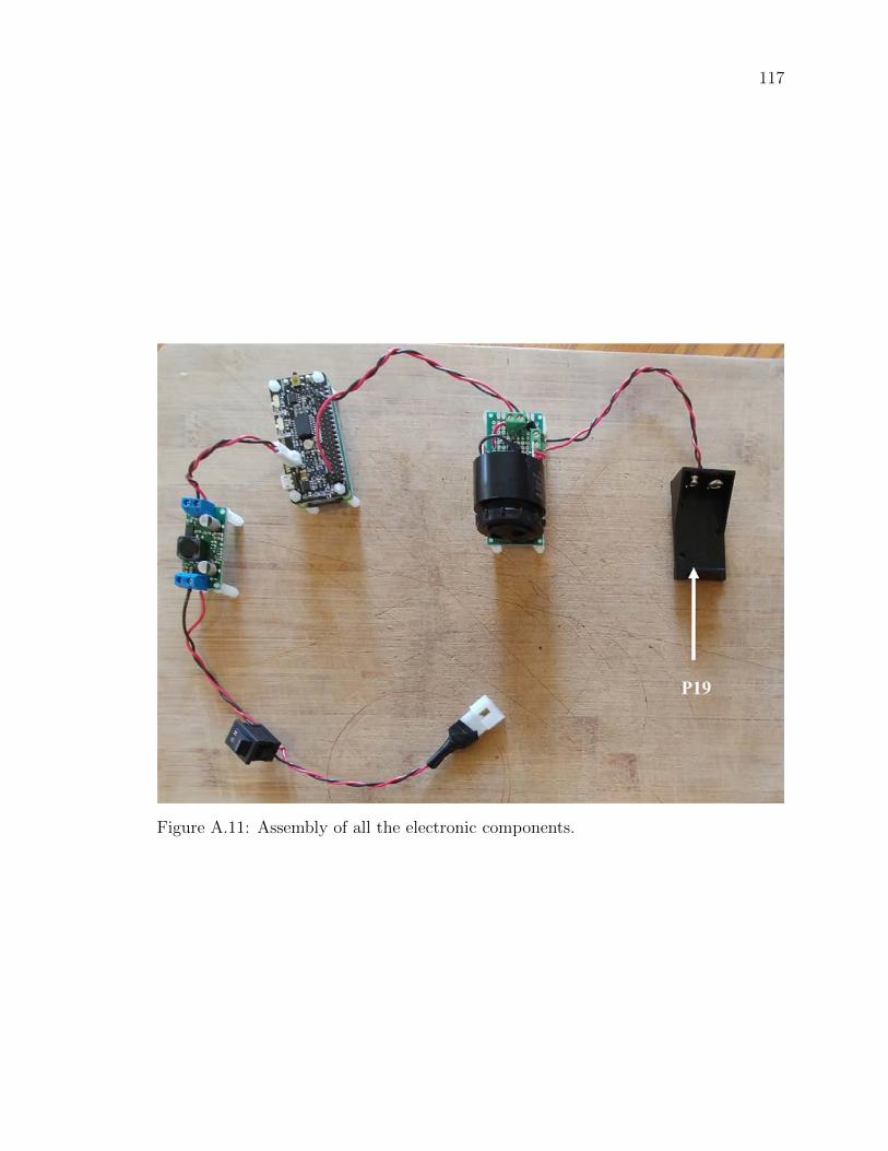
117

Figure A.11: Assembly of all the electronic components.

118

Figure A.12: Placement of the electronic components on the mounting plate.

119

3. Drill all the holes on the mounting plate with a drill and cut the rectangle of

the switch with an exacto knife.

4. Tie a short elastic band through the holes indicated by the orange circles in the

diagram above.

5. Temporarily disconnect all wires of the electronic components from the terminal

blocks.

6. Attach the buzzer circuit and the 9 V battery holder on the bottom side of the

mounting plate with the silicon screws (P10).

7. Attach the voltage regulator, the camera sensor (via the camera holder) and

the Raspberry Pi on the top side of the mounting plate using the silicon screws

(P10). The camera sensor should be placed such that the ribbon cable connector

is on the top side of the mounting plate.

8. Connect the free end of the ribbon cable of the camera to the camera port of

the Raspberry Pi. The cable must go underneath the Raspberry Pi and be held

down by the elastic band.

9. Glue the ON/OFF switch to the mounting plate.

10. Reconnect all the wires to their respective terminal blocks (Figure A.13).

A.2.2 Building the internal frame

The internal frame holds the battery pack and the electronic components in the 4”

diameter tube of the pressure housing. The steps to assemble the internal frame are

as follows.

1. Draw a disc of diameter 4” on the PVC vinyl tile (P30) and cut it out with an

exacto knife (Figure A.14).

2. Use sand paper to smooth the edges of the disc (Figure A.15). Ensure it fits

perfectly into the tube of the pressure housing (i.e. a 4” diameter tube).

120

Figure A.13: Electronic components installed on the mounting plate.

Figure A.14: Cutting of the discs from the PVC vinyl tile.

121

Figure A.15: Sanding edges of the discs.

Figure A.16: Locating holes to drill on the discs.

122

3. Place seven D-cell batteries perfectly centered on top of the disk. Place eight

nails (or screws) between the D-cell batteries as shown in Figure A.16.

4. Gently tap on the nails with a hammer to leave a mark on the disk. Remove

the batteries and nails, and drill holes with a drill at each mark on the disk.

These holes will be used for holding the rods. The two holes indicated with the

green circles will be for the longer rods going up to the front-view window of

the pressure housing. Drill two additional holes (indicated in red in the figure

below and referred to as “wire holes” in the following steps) large enough to fit

seven wires (Figure A.17).

Figure A.17: Drilling of the holes on the discs.

5. Repeat steps 1-4 twice to obtain three disks. The first disk, referred to as

“positive disk”, will hold all the positive (+) battery connectors (P21 plates).

The second disk, referred to as “negative disk”, will hold all the negative (−)

battery connectors (P21 springs). The third disk, referred to as “connector-free

disk”, will serve as a structural component and will not have any connectors

attached to it. The connector-free disk should not have any cable holes drilled

into it (i.e. red-labeled holes depicted in the figure above).

6. Solder red wires to the seven positive battery connectors (P21 plates), glue them

to the positive disk, and pass the free end of the wires through one of the wire

holes (Figure A.18). The red wires should be ∼ 40 cm long.

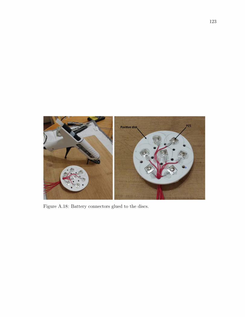
123

Figure A.18: Battery connectors glued to the discs.

124

7. Repeat step 6, but this time using black wires and the negative battery con-

nectors (P21 springs) on the negative disk. The black wires should be ∼ 15 cm

long.

8. With a metal saw cut six 28.6 cm (11.25 inch) rods (P23), and two 40 cm rods

(Figure A.19).

Figure A.19: Cutting of the metal rods.

9. Attach all the rods to the connector-free disk using washers (P24), lock-washers

(P26) and nuts (P25) on both sides. For one of the central rods, the washers,

lock-washers and nuts should only be used on the external side of the disk, so

it can be easily removed when installing the D-cell batteries. The longer 40 cm

rods should be in the outside holes (depicted in green in the figure of step 4)

and the short ones should be in the central holes. b) Pass the red wires of the

positive disk through the second wire hole, then slide the disk through the rods

and stack it on top of the connector-free disk (Figure A.20).

10. Slide the negative disk through the rods with the spring connectors facing the

plate connectors of the positive disk, and secure it to the rods using the washers

(P24), lock-washers (P26) and nuts (P25) on both sides. As for the positive disk,

one of the central rods should have washers, lock-washers and nuts on one side

only to be able to remove the rod easily when installing the D-cell batteries. Use

four D-cell batteries between the centrals rods to ensure the distance between

the positive and negative disks is appropriate (i.e. long enough to fit four D-cell

batteries, but short enough to maintain the D-cell batteries tightly in place).

125

Figure A.20: Assembly of the rods and discs.

126

Finally, pass the red wires from the positive disk through the remaining wire

hole of the negative disk (Figure A.21).

Figure A.21: Assembly of the negative discs.

11. Solder the free end of the red and black wires to the Molex battery connector

(P13, Figure A.22).

Figure A.22: Soldering of the Molex connector.

12. Cut a small piece of metal hanger strap (P31), bend it as a finger handle and

attach it to the outside of the connector-free disk with the washers (P24), lock-

washers (P26) and nuts (P25, Figure A.23).

127

Figure A.23: Attachment of the handle.

128

13. Slide the mounting plate with the electronics through the rods (Figure A.24).

Figure A.24: Assembly of the electronics with the internal frame.

14. Secure the mounting plate to the rods with four small cable ties (P32) and

connect the board to the battery pack with the Molex battery connectors (P13,

Figure A.25).

Figure A.25: Connection of the electronics to the battery pack.

15. Add a nut (P25), lock-washer (P25), and cap nut (P27) to the end of the two

long rods and cover the cap nut with a screw protector (P28, Figure A.26).

16. The inside of the FishCam is now assembled (Figure A.27).

129

Figure A.26: Assembly of the cap nut and screw protector.

Figure A.27: Inside of the Fishcam fully assembled.

130

A.2.3 Building the pressure housing and external attach-

ment

All the instructions to build the custom PVC housing are in the supplementary ma-

terial of Bergshoeff et al. [98]. The off-the-shelf 4” pressure housing can easily be

ordered from the Blue Robotics website (https://bluerobotics.com/store/watertight-

enclosures/4-series/wte4-asm-r1/).

The external attachment for the FishCam is assembled as follows.

1. Using a saw, cut an ABS 4” × 4” × 2” tee fitting (P35) in half, lengthwise

(Figure A.28).

Figure A.28: Cutting of the tee fitting.

2. Glue a 2” to 1-1/2” flush bushing fitting (P36) to the tee fitting using PVC

cement (Figure A.29).

3. a) Cut a small piece of 1-1/2” PVC pipe (P38) and attach it to the PVC union

fitting (P37) using PVC cement. b) Attach the PVC union to the tee fitting

using PVC cement (Figure A.30).

4. Repeat steps 1-3.

5. Place the two halves of tee fittings on either side of the pressure housing and

secure with three adjustable stainless steel collars (P39, Figure A.31).

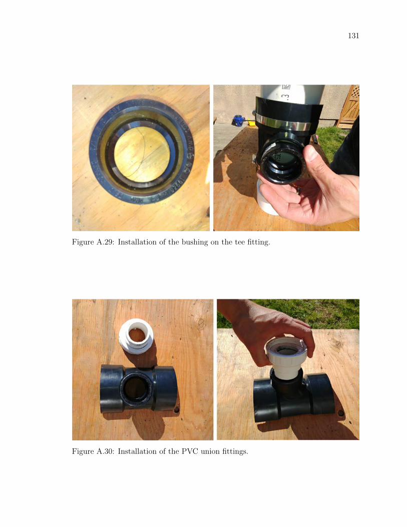
131

Figure A.29: Installation of the bushing on the tee fitting.

Figure A.30: Installation of the PVC union fittings.

132

Figure A.31: Installation of PVC attachments to the pressure housing of the Fishcam.

A.2.4 Installing the D-cell batteries

This section describes the steps to install the D-cell batteries in the FishCam.

1. Test with a voltmeter that all the D-cell batteries are properly charged.

2. Unscrew the end of one of the central rods (the one with no bolts on the inside

of the negative disk) and slide it out. Insert the four D-cell batteries in the

central battery stack. Slide the rod back and secure it with the bolts and nuts

(Figure A.32).

3. Wrap the laminated plastic sheet (P29) around the rods and hold it in place

with your hand.

4. Slide the plastic sheet down towards the positive-disk and insert the first row

of 6 batteries.

133

Figure A.32: Installation of the D-cell batteries in the central stack.

134

5. Slide the plastic sheet slightly up and insert the second row of batteries. Repeat

this process for the third and fourth rows of batteries.

6. Hold the plastic sheet tightly around the battery pack with your hand and use

electrical tape to keep it in place. At this point the batteries should be well

secured and not moving (Figure A.33).

Figure A.33: Installation of the rest of the D-cell batteries.

7. Measure the voltage of each 4-battery stack with a voltmeter. All stacks should

have the same voltage value.

135

A.3 Operation instructions

This section describes how to set the FishCam to start recording when it is powered

ON and how to adjust the video settings (frame rate, ISO, resolution, etc). For these

instructions you need to have the FishCam started and have access to the FishCam OS

either directly via a mouse, keyboard and monitor, or remotely via an SSH connection

(see section A.3.7).

A.3.1 Installing the software suite

Setting up the software requires both a computer and the FishCam. It is assumed

here that the computer is using a recent version of the Microsoft Windows operating

system (OS). Using a computer with a different OS is possible but is not documented

here. It is also assumed that a Wifi connection with access to the internet is available.

Steps 1-6 are performed on the Windows computer, and steps 7-14 are performed on

the FishCam itself. For all these steps, it is recommended to power the FishCam via

the power USB port of the Raspberry Pi using an external power supply (i.e. not the

D-cell battery pack).

1. Take the microSD card (P9) and connect it to your computer.

2. Use free software such as SD Card Formatter to format the microSD card.

3. Download the image (.img) file Raspbian Buster with Desktop from the Rasp-

berry Pi website

(https://www.raspberrypi.org/downloads/raspbian/).

4. Copy the Raspbian image to the microSD card using free software such as Win32

Disk Imager.

5. Once Raspbian is installed on the microSD card it will appear on the computer

as two separate drives boot and rootfs. On the boot drive, open the file config.txt

with a text editor (e.g. Notepad) and add the line dtoverlay=pi3-disable-bt at

the end of the file. Save and close the text editor. This step turns off the

Bluetooth capabilities of the Raspberry Pi to save power. Ignore this step if

you need to use the Bluetooth.

6. Eject the microSD card from the computer and insert it in the FishCam’s Rasp-

berry Pi.

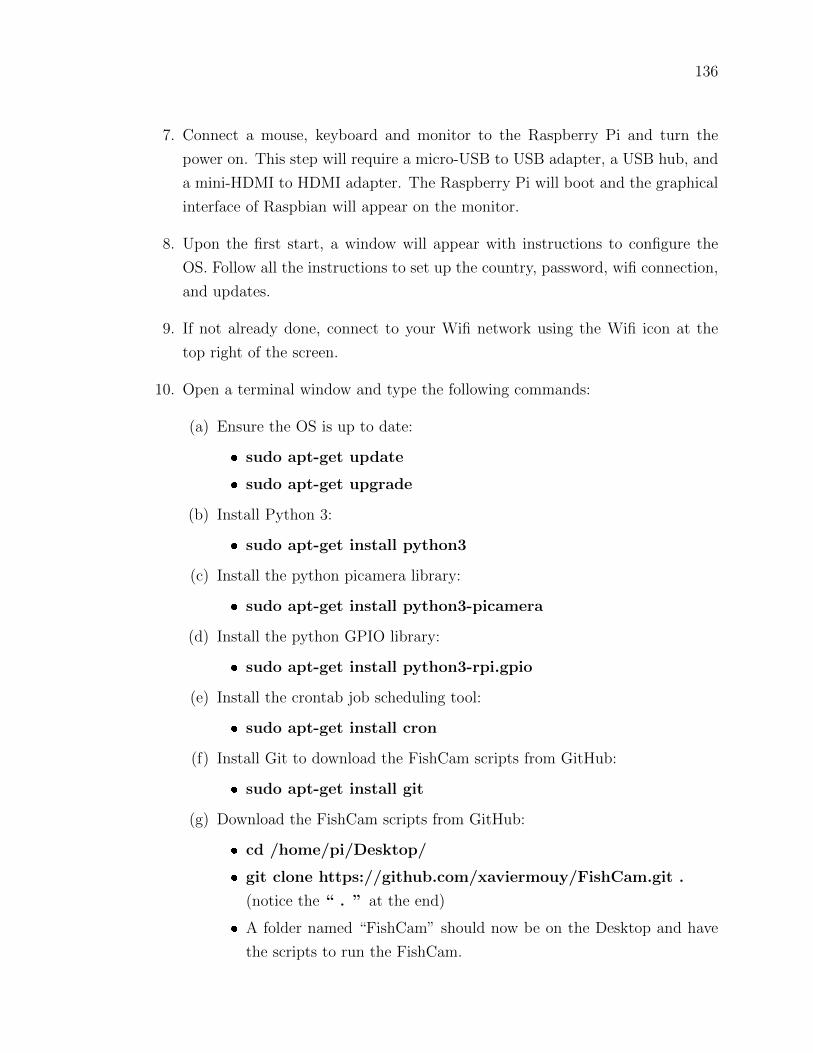
136

7. Connect a mouse, keyboard and monitor to the Raspberry Pi and turn the

power on. This step will require a micro-USB to USB adapter, a USB hub, and

a mini-HDMI to HDMI adapter. The Raspberry Pi will boot and the graphical

interface of Raspbian will appear on the monitor.

8. Upon the first start, a window will appear with instructions to configure the

OS. Follow all the instructions to set up the country, password, wifi connection,

and updates.

9. If not already done, connect to your Wifi network using the Wifi icon at the

top right of the screen.

10. Open a terminal window and type the following commands:

(a) Ensure the OS is up to date:

sudo apt-get update

sudo apt-get upgrade

(b) Install Python 3:

sudo apt-get install python3

(c) Install the python picamera library:

sudo apt-get install python3-picamera

(d) Install the python GPIO library:

sudo apt-get install python3-rpi.gpio

(e) Install the crontab job scheduling tool:

sudo apt-get install cron

(f) Install Git to download the FishCam scripts from GitHub:

sudo apt-get install git

(g) Download the FishCam scripts from GitHub:

cd /home/pi/Desktop/

git clone https://github.com/xaviermouy/FishCam.git .

(notice the “ . ” at the end)

A folder named “FishCam” should now be on the Desktop and have

the scripts to run the FishCam.

137

(h) Install the WittyPi software:

wget http://www.uugear.com/repo/WittyPi2/installWittyPi.sh

sudo sh installWittyPi.sh

When prompted, type y to remove fake-hwclock, and n to not install

Qt5

11. Restart the Raspberry Pi to apply all the changes.

12. Once Raspbian has restarted, open a terminal window and type sudo raspi-

config to configure the Raspberry Pi:

(a) If not done already, change your user password in the menu Change User

Password.

(b) In the menu Network Options select Hostname, and change it to fish-

cam01. Other hostnames can be chosen, but it has to be explicit enough

to be easily identifiable on a network.

(c) In the menu Change Boot Options and Desktop/CLI, select Desktop

Auto Login.

(d) To set FishCam time to UTC, in the menu Localisation Options, select

Change Time Zone, then None, and GMT.

(e) In the menu Interfacing Options set the Camera (CSI camera inter-

face) and SSH connection to enabled.

(f) Ensure the entire microSD card is used by selecting Expand Filesystem

in the menu Advanced Options.

(g) Select Finish to exit raspi-config.

13. At this point all the necessary software are installed.

14. Optional: shut down the Raspberry Pi, take the microSD card out and connect

it to your computer. Use free software such as Win32 Disk Imager to take

an image of the microSD card with all the software installed. The image file

created may be used to set up another FishCam without having to go through

all the installation steps described above.

138

A.3.2 Automatic start of the recordings

The crontab job scheduler is used to start acquiring video when the FishCam is pow-

ered ON (i.e. rebooted). Open a terminal window and type the following commands:

1. Edit the job schedule by typing: crontab -e

2. The first time you run crontab you will be prompted to select an editor. Choose

Nano by pressing Enter.

3. Once the schedule is open in Nano:

(a) Scroll down with the down-arrow key to the bottom of the document and

type

@ reboot sh /home/pi/Desktop/FishCam/script/camStartup.sh

&

(b) Save the changes by pressing CTRL + O, then press Enter to confirm.

(c) Exit Nano by pressing CTRL + X.

4. Verify that the schedule has been saved:

crontab -l

5. Close terminal

A.3.3 FishCam ID

If you are using several FishCams, it may be useful to assign a unique ID to each

of them. This ID will be used at the beginning of the filename of each video being

recorded. To modify the FishCam ID:

1. Go to the folder /home/pi/Desktop/FishCam/script/

2. Open the file FishCamID.config with a text editor.

3. Type the FishCam ID, save, and close the text editor. By default FishCam ID

is set to FishCam01.

139

A.3.4 Camera settings

All the camera settings are defined in the python script captureVideo.py located in

the folder /home/pi/Desktop/FishCam/script/. To change the settings, open

the script captureVideo.py with a text editor and adjust the parameters defined in

the function initVideoSettings(). For more information about the different parame-

ters, refer to the documentation of the picamera library [101].

def i n i tV i d e oS e t t i n g s ( ) :

v i d eoSe t t i ng s = ’ durat ion ’ : 300 , # f i l e s dura t ion in sec

’ r e s o l u t i o n ’ : (1600 ,1200) ,

’ frameRate ’ : 10 , # frame ra t e f p s

’ q ua l i t y ’ : 20 , # 1 = be s t q ua l i t y , 30 poorer q u a l i t y

’ format ’ : ’ h264 ’ , # ’ h264 ’ , ’mjpeg ’

’ exposure ’ : ’ n ight ’ , # ’ auto ’ , ’ n i gh t ’ , ’ b a c k l i g h t ’

’AWB’ : ’ auto ’ , # ’ auto ’ , ’ c loudy ’ , ’ s u n l i g h t ’

’ sharpness ’ : 0 , # in t e g e r between =100 and 100 , auto : 0

’ c on t ra s t ’ : 0 , # in t e g e r between =100 and 100 , auto : 0

’ b r i gh tne s s ’ : 50 , # in t e g e r between 0 and 100 , auto : 0

’ s a tu ra t i on ’ : 0 , # in t e g e r between =100 and 100 , auto : 0

’ ISO ’ : 400 , # auto : 0

’ v f l i p ’ : Fa l se

return v id eoSe t t i ng s

A.3.5 Configuring the duty cycles

The duty cycles of the FishCam are configured with the software provided with the

Witty Pi and installed in section A.3.1. In this section, it is assumed that the FishCam

is connected to the internet via Wifi.

1. Create a Witty Pi schedule script (i.e. .wpi file) to define the ON and OFF

sequence needed and save it in the folder /home/pi/WittyPi/schedules/. The

name of the .wpi file should be explicit and self-explanatory (e.g. textitschedule_

fishcam_fall_UTC.wpi). Examples of schedule scripts can be found in the

folder textbf/home/pi/Desktop/FishCam/wittypi_schedules/. For more in-

formation on how to define ON/OFF sequences, refer to the Witty Pi user

manual.

140

2. Open a terminal window:

(a) Ensure the clock of the FishCam is at the correct time by typing the

command date. If the date and time displayed are not correct, make

sure that the FishCam is connected to the internet. The time should be

updated automatically once an internet connection is established.

(b) Start the Witty Pi software:

sudo sh /home/pi/WittyPi/wittyPi.sh

(c) Select menu item 3: Synchronize time.

(d) Ensure the system clock and the RTC clock at the top of the menu options

show the same time. If not, re-run the time synchronization.

(e) Select menu item 6: Choose schedule script, and choose the name of

the schedule script you created at the first step.

(f) Select menu item 8: Exit

3. The duty cycles are now activated and the FishCam will start to turn ON and

OFF based on the schedule defined.

Note: The witty Pi mini cannot remember the time (RTC) without power

for more than 17 hours. Consequently, the time synchronization and sched-

ules should be defined no more than 17 hours before the deployment of

the FishCam.

A.3.6 Configuring the buzzer

The beeping sequence of the buzzer can be defined by editing the file /home-

/pi/Desktop/FishCam/script/runBuzzer.py with a text editor. The five pa-

rameters below can be adjusted:

beep dur sec: Duration of a single beep in seconds.

beep gap sec: Duration of the silence between beeps in seconds.

beep number: Number of beeps in a sequence.

number beep sequences: Number of sequences.

gap btw sequences sec: Duration of the silence between sequences.

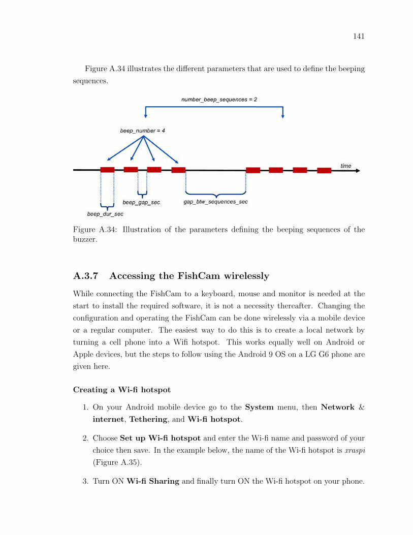
141

Figure A.34 illustrates the different parameters that are used to define the beeping

sequences.

Figure A.34: Illustration of the parameters defining the beeping sequences of thebuzzer.

A.3.7 Accessing the FishCam wirelessly

While connecting the FishCam to a keyboard, mouse and monitor is needed at the

start to install the required software, it is not a necessity thereafter. Changing the

configuration and operating the FishCam can be done wirelessly via a mobile device

or a regular computer. The easiest way to do this is to create a local network by

turning a cell phone into a Wifi hotspot. This works equally well on Android or

Apple devices, but the steps to follow using the Android 9 OS on a LG G6 phone are

given here.

Creating a Wi-fi hotspot

1. On your Android mobile device go to the System menu, then Network &

internet, Tethering, and Wi-fi hotspot.

2. Choose Set up Wi-fi hotspot and enter the Wi-fi name and password of your

choice then save. In the example below, the name of the Wi-fi hotspot is xraspi

(Figure A.35).

3. Turn ON Wi-fi Sharing and finally turn ON the Wi-fi hotspot on your phone.

142

Figure A.35: Setting up a Wi-fi hotspot.

143

4. Connect the FishCam to a keyboard, mouse and monitor and turn it on. This

will be the last time you will need to connect the FishCam to a monitor.

5. Once started, click on the Wi-fi icon at the top right of the screen, select your

Wi-fi hotspot (here xraspi) and enter the corresponding password (the one set

in step 2). Now the FishCam should connect to this network automatically if it

is available. To ensure this is actually the case, before taking off the keyboard,

mouse and monitor, you can reboot the FishCam and confirm that it connects

automatically to the Wi-fi hotspot.

6. At this point all the keyboard, mouse, and monitor can be disconnected.

Controlling the FishCam from a mobile device

Several phone applications exist to control the Raspberry Pi. Here we provide in-

structions for the free application RaspController by Ettore Gallina.

1. Turn ON the Wi-fi hotspot on your cell phone.

2. Turn ON the FishCam.

3. On you cell phone go in the menu System, then Network & internet, Teth-

ering, and Wi-fi hotspot.

4. After a moment the FishCam should appear in the “Connected Devices” section.

Note the FishCam’s IP address (in the example in Figure A.36, the IP address

is 192.168.43.95)

5. Start the application RaspController on your phone, add a device (+ sign at the

top right), then enter the IP address and password (the one defined in section

A.3.1) of the FishCam and save.

6. Once connected to the FishCam, you can browse through the folders and files

via the File Manager menu, open a terminal window via the menu Shell

SSH, and monitor the FishCam resources via the menu Cpu, RAM, Disk

monitoring (Figure A.37).

7. Through the File Manager, it is possible to monitor that everything is working

properly by verifying that video files are being recorded in the folder /home-

/pi/Desktop/FishCam/data/, verify their size, and read the logs to ensure all

144

.

Figure A.36: FishCam connected to the wi-fi hotspot.

Figure A.37: RaspController’s interface to control and monitor the FishCam.

145

processes started properly and that there are no errors (Figure A.38).

Figure A.38: Monitoring the status of the data acquisition.

Controlling the FishCam from a computer

The FishCam can also be accessed wirelessly from a computer. While there are several

ways to do this, here we provide instructions using a Wi-fi hotspot (section A.3.7).

1. Turn ON the Wi-fi hotspot on your cell phone.

2. Connect to the Wi-fi hotspot on your computer.

3. Turn ON the FishCam.

4. On your cell phone go into the System menu, then Network & internet,

Tethering, and Wi-fi hotspot.

5. After a moment the FishCam should appear in the “Connected Devices” section.

Note the FishCam’s IP address.

6. On your computer, use a SFTP client such as FileZilla to connect to the Fish-

Cam and browse through the folders and files. You will need to connect using

the FishCam’s IP address, username (i.e. “pi”), password (the one defined in

section A.3.1) and using the port 22.

146

7. On your computer, use an SSH client such as Putty to access the terminal

console of the FishCam. You will also need to connect using the FishCam’s IP

address, username, password, use port 22 and an SSH connection type.

A.3.8 Downloading data from the FishCam

The fastest way to download the data from the FishCam, is to take the microSD

card out, connect it to a computer, and copy the data and logs folders to the com-

puter. It is also possible to connect wirelessly to the FishCam from a computer and

transfer the data via a SFTP client software (see section A.3.7). It is recommended

to download both the data folder, which contains all the video files, and the logs

folder, which contains information about the start time of the buzzer sequences and

any errors that may have occurred during the data acquisition.

Data folder:

/home/pi/Desktop/FishCam/data/

Logs folder:

/home/pi/Desktop/FishCam/logs/

A.3.9 Pre-deployment checklist

In order to minimize failures, it is recommended to go through the following steps

before deploying the FishCam in the field.

D-cell batteries at least 1.4 V.

All wires properly connected and undamaged.

Camera ribbon connector properly attached/not loose.

Camera lens clean and free of debris.

Buzzer’s 9 V battery connected.

O-rings of the pressure housing clean and greased with lube.

Front-view window clean.

Time on the FischCam’s clock is correct (check with the command ”date” in

an SSH terminal).

147

RTC of the WittyPi is synchronized and ON/OFF schedule is operational.

Buzzer rang after power turned ON.

Files recording properly (check number of files recorded, file sizes and logs via

SSH).

148

Bibliography

1Aristotle, The Complete Works of Aristotle-The Revised Oxford Translation II

(Princeton, N.J: Princeton University Press, 1984).

2M. Dufosse, “Recherches sur les bruits et les sons expressifs que font entendre les

poissons d’Europe et sur les organes producteurs de ces phenomenes acoustiques

ainsi que sur les appareils de l’audition de plusieurs de ces animaux”, Ann. Sci.

Nat. 19, 1–53 (1874).

3J. Muller, “Beobachtungen uber die Schwimmblase der Fische, mit Bezug auf einige

neue Fischgattungen”, Arch. Anat. Physiol. 1842, 307–329 (1842).

4M. P. Fish, Sonic fishes of the Pacific. Tech. rep. (Woods Hole Oceanographic

Institution, WHOI Technical report n°2., 1948).

5M. P. Fish, “The character and significance of sound production among fishes of

the western North Atlantic.”, Bingham Oceanogr. Collect. Bull. 14, 1–109 (1954).

6M. P. Fish and W. H. Mowbray, Sounds of western North Atlantic fishes: a refer-

ence file of biological underwater sounds (Johns Hopkins Press, Baltimore, 1970).

7P. Cousteau and P. Watson, The Undersea World of Jacques Cousteau: Savage

Worlds of the Coral Jungle. 1968.

8I. Kaatz, “Multiple sound-producing mechanisms in teleost fishes and hypotheses

regarding their behavioural significance”, Bioacoustics 12, 230–233 (2002).

9R. A. Rountree, G. Gilmore, C. A. Goudey, A. D. Hawkins, J. J. Luczkovich,

and D. A. Mann, “Listening to Fish: applications of passive acoustics to fisheries

science”, Fisheries 31, 433–446 (2006).

10C. C. Wall, R. A. Rountree, C. Pomerleau, and F. Juanes, “An exploration for deep-

sea fish sounds off Vancouver Island from the NEPTUNE Canada ocean observing

system”, Deep. Res. Part I 83, 57–64 (2014).

https://doi.org/10.1080/09524622.2002.9753705

https://doi.org/10.1577/1548-8446(2006)31

https://doi.org/10.1016/j.dsr.2013.09.004

149

11M. C. P. Amorim, Y. Stratoudakis, and A. D. Hawkins, “Sound production during

competitive feeding in the grey gurnard”, J. Fish Biol. 65, 182–194 (2004).

12J. M. Moulton, “Swimming sounds and the schooling of fishes”, Biol. Bull. 119,

210–223 (1960).

13A. H. Bass and F. Ladich, “Vocal–Acoustic Communication: From Neurons to

Behavior”, in Fish bioacoustics , edited by J. F. Webb, R. R. Fay, and A. N. Popper

(Springer New York, New York, NY, 2008), pp. 253–278.

14F. Ladich and A. A. Myrberg, “Agonistic behaviour and acoustic communication”,

in Commun. fishes, edited by K. B. G. Ladich F., Collin S. P., Moller P. (Science

Publishers, 2006), pp. 122–148.

15E. W. Montie, C. Kehrer, J. Yost, K. Brenkert, T. O’Donnell, and M. R. Denson,

“Long-term monitoring of captive red drum Sciaenops ocellatus reveals that calling

incidence and structure correlate with egg deposition”, J. Fish Biol. 88, 1776–95

(2016).

16M. C. P. Amorim, R. O. Vasconcelos, and P. J. Fonseca, “Fish Sounds and Mate

Choice”, in Sound commun. fishes , edited by F. Ladich (Springer Vienna, Vienna,

2015), pp. 1–33.

17W. N. Tavolga, “Mechanisms for directional hearing in the sea catfish (Arius fe-

lis).”, J. Exp. Biol. 67, 97–115 (1977).

18P. S. Lobel, “Sounds produced by spawning fishes”, Environ. Biol. Fishes 33, 351–

358 (1992).

19E. Parmentier, J. P. Lagardere, P. Vandewalle, and M. L. Fine, “Geographical

variation in sound production in the anemonefish Amphiprion akallopisos”, Proc.

R. Soc. B Biol. Sci. 272, 1697–703 (2005).

20J. J. Luczkovich, R. C. Pullinger, S. E. Johnson, and M. W. Sprague, “Identifying

Sciaenid Critical Spawning Habitats by the Use of Passive Acoustics”, Trans. Am.

Fish. Soc. 137, 576–605 (2008).

21C. B. Portt, G. A. Coker, D. L. Ming, and R. G. Randall, A review of fish sampling

methods commonly used in Canadian freshwater habitats. Tech. rep. (Canadian

Technical Report of Fisheries and Aquatic Sciences, 2006), p. 58.

https://doi.org/10.1111/j.0022-1112.2004.00443.x

https://doi.org/10.1097/00003446-199510000-00013

https://doi.org/10.1111/jfb.12938


https://doi.org/10.1007/978-3-7091-1846-7_1

https://doi.org/10.1098/rspb.2005.3146

https://doi.org/10.1098/rspb.2005.3146

https://doi.org/10.1577/T05-290.1

https://doi.org/10.1577/T05-290.1

150

22O. R. Godøl, N. O. Handegard, H. I. Browman, G. J. Macaulay, S. Kaartvedt,

J. Giske, E. Ona, G. Huse, and E. Johnsen, “Marine ecosystem acoustics (MEA):

Quantifying processes in the sea at the spatio-temporal scales on which they occur”,

ICES J. Mar. Sci. 71, 2357–2369 (2014).

23S. J. Pittman, M. E. Monaco, A. M. Friedlander, B. Legare, R. S. Nemeth, M. S.

Kendall, M. Poti, R. D. Clark, L. M. Wedding, and C. Caldow, “Fish with chips:

Tracking reef fish movements to evaluate size and connectivity of Caribbean marine

protected areas”, PLoS One 9, 1–11 (2014).

24A. Riera, R. A. Rountree, M. K. Pine, and F. Juanes, “Sounds of Arctic cod

(Boreogadus saida) in captivity: A preliminary description”, J. Acoust. Soc. Am.

143, 1–6 (2018).

25A. Riera, R. A. Rountree, L. Agagnier, and F. Juanes, “Sablefish (Anoplopoma fim-

bria) produce high frequency rasp sounds with frequency modulation”, J. Acoust.

Soc. Am. 147, 2295–2301 (2020).

26A Sirovic, G. Cutter, L Butler, and D. Demer, “Rockfish sounds and their potential

use for population monitoring in the Southern California Bight”, ICES J. Mar. Sci.

66, 981–990 (2009).

27D. A. Mann, J. Locascio, M. Scharer, M. Nemeth, and R. Appeldoorn, “Sound

production by red hind epinephelus guttatus in spatially segregated spawning ag-

gregations”, Aquat. Biol. 10, 149–154 (2010).

28P. A. Cott, A. D. Hawkins, D. Zeddies, B. Martin, T. A. Johnston, J. D. Reist,

J. M. Gunn, and D. M. Higgs, “Song of the burbot: Under-ice acoustic signaling

by a freshwater gadoid fish”, J. Great Lakes Res. 40, 435–440 (2014).

29M. W. Sprague and J. J. Luczkovich, “Measurement of an individual silver perch

Bairdiella chrysoura sound pressure level in a field recording.”, J. Acoust. Soc. Am.

116, 3186–3191 (2004).

30R. A. Rountree and F. Juanes, “First attempt to use a remotely operated vehicle

to observe soniferous fish behavior in the Gulf of Maine, Western Atlantic Ocean”,

Curr. Zool. 56, 90–99 (2010).

31J. V. Locascio and M. L. Burton, “A passive acoustic survey of fish sound pro-

duction at Riley’s Hump within Tortugas South Ecological Reserve; implications

regarding spawning and habitat use”, Fish. Bull. 114, 103–116 (2015).

https://doi.org/10.1093/icesjms/fsu116

https://doi.org/10.1371/journal.pone.0096028

https://doi.org/10.1121/1.5035162

https://doi.org/10.1121/1.5035162

https://doi.org/10.1121/10.0001071

https://doi.org/10.1121/10.0001071

https://doi.org/10.3354/ab00272

https://doi.org/10.1016/j.jglr.2014.02.017

https://doi.org/10.1121/1.1802651

https://doi.org/10.1121/1.1802651

https://doi.org/10.7755/FB.114.1.9

151

32A. Sirovic, S. Brandstatter, and J. A. Hildebrand, “Fish recordings from NEP-

TUNE Canada”, J. Acoust. Soc. Am. 132, 1916 (2012).

33O. Adam and F. Samaran, Detection, Classification and Localization of Marine

Mammals using passive acoustics, 2003- 2013: 10 years of international research

(Dirac NGO, Paris, France, 2013), p. 298.

34W. M. X Zimmer, Passive Acoustic Monitoring of Cetaceans (Cambridge Univer-

sity Press, Cambridge, UK, 2011), p. 356.

35G. L. D’Spain and H. H. Batchelor, “Observations of biological choruses in the

Southern California Bight: A chorus at midfrequencies”, J. Acoust. Soc. Am. 120,

1942–1955 (2006).

36D. A. Mann and S. M. Jarvis, “Potential sound production by a deep-sea fish”, J.

Acoust. Soc. Am. 115, 2331–2333 (2004).

37J. L. Spiesberger and K. M. Fristrup, “Passive Localization of Calling Animals and

Sensing of their Acoustic Environment Using Acoustic Tomography”, Am. Nat.

135, 107–153 (1990).

38M. J. Parsons, R. D. McCauley, M. C. Mackie, P. Siwabessy, and A. J. Duncan,

“Localization of individual mulloway (Argyrosomus japonicus) within a spawning

aggregation and their behaviour throughout a diel spawning period”, ICES J. Mar.

Sci. 66, 1007–1014 (2009).

39M. J. Parsons, R. D. McCauley, M. C. Mackie, and A. J. Duncan, “A comparison

of techniques for ranging close-proximity mulloway (Argyrosomus Japonicus) calls

with a single hydrophone”, Acoust. Aust. 38, 145–151 (2010).

40J. V. Locascio and D. A. Mann, “Localization and source level estimates of black

drum (Pogonias cromis) calls”, J. Acoust. Soc. Am. 130, 1868–1879 (2011).

41B. G. Ferguson and J. L. Cleary, “In situ source level and source position estimates

of biological transient signals produced by snapping shrimp in an underwater en-

vironment”, J. Acoust. Soc. Am. 109, 3031–3037 (2001).

42Y. M. Too, M. Chitre, G. Barbastathis, and V. Pallayil, “Localizing Snapping

Shrimp Noise Using a Small-Aperture Array”, IEEE J. Ocean. Eng. 44, 207 –219

(2019).

https://doi.org/10.1121/1.4755031

https://doi.org/10.1121/1.2338802

https://doi.org/10.1121/1.2338802

https://doi.org/10.1121/1.1694992

https://doi.org/10.1121/1.1694992

https://doi.org/10.1086/285035

https://doi.org/10.1086/285035

https://doi.org/10.1093/icesjms/fsp016

https://doi.org/10.1093/icesjms/fsp016

https://doi.org/10.1121/1.3621514

https://doi.org/10.1121/1.1339823

https://doi.org/10.1109/JOE.2017.2777718

https://doi.org/10.1109/JOE.2017.2777718

152

43C. A. Radford, S. Ghazali, A. G. Jeffs, and J. C. Montgomery, “Vocalisations of

the bigeye Pempheris adspersa: characteristics, source level and active space”, J.

Exp. Biol. 218, 940–948 (2015).

44B. R. Rountree, “Do you hear what I hear? Future technological development –

and needs- in passive acoustics underwater observation”, Mar. Technol. Report.

51, 40–46 (2008).

45G. E. Davis, M. F. Baumgartner, J. M. Bonnell, J. Bell, C. Berchok, J. Bort

Thornton, S. Brault, G. Buchanan, R. A. Charif, D. Cholewiak, C. W. Clark,

P. Corkeron, J. Delarue, K. Dudzinski, L. Hatch, J. Hildebrand, L. Hodge, H.

Klinck, S. Kraus, B. Martin, D. K. Mellinger, H. Moors-Murphy, S. Nieukirk, D. P.

Nowacek, S. Parks, A. J. Read, A. N. Rice, D. Risch, A. Sirovic, M. Soldevilla, K.

Stafford, J. E. Stanistreet, E. Summers, S. Todd, A. Warde, and S. M. Van Parijs,

“Long-term passive acoustic recordings track the changing distribution of North

Atlantic right whales (Eubalaena glacialis) from 2004 to 2014”, Sci. Rep. 7, 1–12

(2017).

46D. P. Gannon, “Passive Acoustic Techniques in Fisheries Science: A Review and

Prospectus”, Trans. Am. Fish. Soc. 137, 638–656 (2008).

47S. M. Van Parijs, C. W. Clark, R. S. Sousa-Lima, S. E. Parks, S. Rankin, D. Risch,

and I. C. Van Opzeeland, “Management and research applications of real-time and

archival passive acoustic sensors over varying temporal and spatial scales”, Mar.

Ecol. Prog. Ser. 395, 21–36 (2009).

48M. Bolgan, J. O’Brien, E. Chorazyczewska, I. J. Winfield, P. McCullough, and

M. Gammell, “The soundscape of Arctic Charr spawning grounds in lotic and

lentic environments: can passive acoustic monitoring be used to detect spawning

activities?”, Bioacoustics 27, 57–85 (2017).

49S. K. Lowerre-Barbieri, K Ganias, F Saborido-Rey, H Murua, and J. R. Hunter,

“Reproductive timing in marine fishes: variability, temporal scales, and methods”,

Mar. Coast. Fish. 3, 71–91 (2011).

50M. J. Parsons, C. P. Salgado-Kent, S. A. Marley, A. N. Gavrilov, and R. D. Mc-

Cauley, “Characterizing diversity and variation in fish choruses in Darwin Har-

bour”, ICES J. Mar. Sci. 73, 2058–2074 (2016).

51M. J. G. Parsons, C. P. Salgado Kent, A. Recalde-Salas, and R. D. McCauley, “Fish

choruses off Port Hedland, Western Australia”, Bioacoustics 4622, 1–18 (2017).

https://doi.org/10.1242/jeb.115295

https://doi.org/10.1242/jeb.115295

https://doi.org/10.1038/s41598-017-13359-3

https://doi.org/10.1038/s41598-017-13359-3

https://doi.org/10.1577/T04-142.1

https://doi.org/10.3354/meps08123


https://doi.org/10.1080/09524622.2017.1286262

https://doi.org/10.1080/19425120.2011.556932

https://doi.org/10.1093/icesjms/fsw037

https://doi.org/10.1080/09524622.2016.1227940

153

52I. Sanchez-Gendriz and L. R. Padovese, “A methodology for analyzing biologi-

cal choruses from long-term passive acoustic monitoring in natural areas”, Ecol.

Inform. 41, 1–10 (2017).

53L. Di Iorio, X. Raick, E. Parmentier, P. Boissery, C. A. Valentini-Poirier, and C.

Gervaise, “’Posidonia meadows calling’: A ubiquitous fish sound with monitoring

potential”, Remote Sens. Ecol. Conserv. 4, 248–263 (2018).

54E. Parmentier, L. Di Iorio, M. Picciulin, S. Malavasi, J.-P. Lagardere, and F.

Bertucci, “Consistency of spatiotemporal sound features supports the use of passive

acoustics for long-term monitoring”, Anim. Conserv. 21, 211–220 (2017).

55R. A. Rountree and F. Juanes, “Potential of passive acoustic recording for moni-

toring invasive species: freshwater drum invasion of the Hudson River via the New

York canal system”, Biol. Invasions 19, 2075–2088 (2017).

56D. P. Gannon and J. G. Gannon, “Assessing trends in the density of Atlantic

croaker (Micropogonias undulatus): A comparison of passive acoustic and trawl

methods”, Fish. Bull. 108, 106–116 (2010).

57T. J. Rowell, M. T. Scharer, R. S. Appeldoorn, M. I. Nemeth, D. A. Mann, and

J. A. Rivera, “Sound production as an indicator of red hind density at a spawning

aggregation”, Mar. Ecol. Prog. Ser. 462, 241–250 (2012).

58T. J. Rowell, D. A. Demer, O. Aburto-Oropeza, J. J. Cota-Nieto, J. R. Hyde,

and B. E. Erisman, “Estimating fish abundance at spawning aggregations from

courtship sound levels”, Sci. Rep. 7, 1–14 (2017).

59D. Gillespie, “Detection and classification of right whale calls using an ”edge”

detector operating on a smoothed spectrogram.”, Can. Acoust. 32, 39–47 (2004).

60D. K. Mellinger and C. W. Clark, “Recognizing transient low-frequency whale

sounds by spectrogram correlation.”, J. Acoust. Soc. Am. 107, 3518–3529 (2000).

61X. Mouy, J. Oswald, D. Leary, J. Delarue, J. Vallarta, B. Rideout, D. Mellinger, C.

Erbe, D. Hannay, and B. Martin, “Passive acoustic monitoring of marine mammals

in the Arctic”, in Detect. classif. localization mar. mamm. using passiv. acoust.

Edited by O. Adam and F. Samaran (Dirac NGO, Paris, France, 2013) Chap. 9.

62M. A. Roch, M. S. Soldevilla, J. C. Burtenshaw, E. E. Henderson, and J. A. Hilde-

brand, “Gaussian mixture model classification of odontocetes in the Southern Cal-

ifornia Bight and the Gulf of California”, J. Acoust. Soc. Am. 121, 1737–1748

(2007).

https://doi.org/10.1016/j.ecoinf.2017.07.001


https://doi.org/10.1002/rse2.72

https://doi.org/10.1111/acv.12362

https://doi.org/10.1007/s10530-017-1419-z


https://doi.org/10.1038/s41598-017-03383-8

https://doi.org/10.1121/1.429434

https://doi.org/10.1121/1.2400663

https://doi.org/10.1121/1.2400663

154

63A. M. Thode, K. H. Kim, S. B. Blackwell, C. R. Greene, C. S. Nations, T. L. Mc-

Donald, and A. M. Macrander, “Automated detection and localization of bowhead

whale sounds in the presence of seismic airgun surveys.”, J. Acoust. Soc. Am. 131,

3726–47 (2012).

64I. R. Urazghildiiev and C. W. Clark, “Acoustic detection of North Atlantic right

whale contact calls using spectrogram-based statistics”, J. Acoust. Soc. Am. 122,

769–76 (2007).

65D. A. Mann, A. A. D. Hawkins, and J. M. Jech, “Active and Passive Acoustics to

Locate and Study Fish”, in Fish bioacoustics , edited by J. F. Webb, R. R. Fay,

and A. N. Popper (Springer New York, New York, NY, 2008), pp. 279–309.

66D. A. Mann and P. S. Lobel, “Passive acoustic detection of sounds produced by the

damselfish, Dascyllus albisella (Pomacentridae)”, Bioacoustics 6, 199–213 (1995).

67R. Stolkin, S. Radhakrishnan, A. Sutin, and R. Rountree, “Passive acoustic detec-

tion of modulated underwater sounds from biological and anthropogenic sources”,

in Ocean. 2007 (2007), pp. 1–8.

68A. K. Ibrahim, L. M. Cherubin, H. Zhuang, M. T. Scharer Umpierre, F. Dalgleish,

N. Erdol, B. Ouyang, and A. Dalgleish, “An approach for automatic classification

of grouper vocalizations with passive acoustic monitoring”, J. Acoust. Soc. Am.

143, 666–676 (2018).

69M. Malfante, J. I. Mars, M. Dalla Mura, and C. Gervaise, “Automatic fish sounds

classification”, J. Acoust. Soc. Am. 139, 2115–2116 (2018).

70J. J. Noda, C. M. Travieso, and D. Sanchez-Rodrıguez, “Automatic Taxonomic

Classification of Fish Based on Their Acoustic Signals”, Appl. Sci. 6, 443 (2016).

71M. Vieira, P. J. Fonseca, M. C. P. Amorim, and C. J. Teixeira, “Call recognition

and individual identification of fish vocalizations based on automatic speech recog-

nition: An example with the Lusitanian toadfish”, J. Acoust. Soc. Am. 138, 3941–

3950 (2015).

72F. Sattar, S. Cullis-Suzuki, and F. Jin, “Acoustic analysis of big ocean data to

monitor fish sounds”, Ecol. Inform. 34, 102–107 (2016).

73I. R. Urazghildiiev and S. M. Van Parijs, “Automatic grunt detector and recognizer

for Atlantic cod (Gadus morhua)”, J. Acoust. Soc. Am. 139, 2532–2540 (2016).

https://doi.org/10.1121/1.3699247

https://doi.org/10.1121/1.3699247

https://doi.org/10.1121/1.2747201

https://doi.org/10.1121/1.2747201

https://doi.org/10.1007/978-0-387-73029-5_9

https://doi.org/10.1080/09524622.1995.9753290

https://doi.org/10.1109/OCEANS.2007.4449200

https://doi.org/10.1121/1.5022281

https://doi.org/10.1121/1.5022281

https://doi.org/10.1121/1.5036628

https://doi.org/10.3390/app6120443

https://doi.org/10.1121/1.4936858

https://doi.org/10.1121/1.4936858


https://doi.org/10.1121/1.4948569

155

74T.-H. Lin, Y. Tsao, and T. Akamatsu, “Comparison of passive acoustic soniferous

fish monitoring with supervised and unsupervised approaches”, J. Acoust. Soc.

Am. 143, EL278–EL284 (2018).

75T. H. Lin, S. H. Fang, and Y. Tsao, “Improving biodiversity assessment via unsu-

pervised separation of biological sounds from long-duration recordings”, Sci. Rep.

7, 1–10 (2017).

76X. Mouy, R. Rountree, F. Juanes, and S. Dosso, “Cataloging fish sounds in the

wild using combined acoustic and video recordings”, J. Acoust. Soc. Am. 143,

EL333–EL333 (2018).

77A. O. Kasumyan, “Sounds and sound production in fishes”, J. Ichthyol. 48, 981–

1030 (2008).

78A. Sirovic and D. A. Demer, “Sounds of captive rockfishes”, Copeia 2009, 502–509

(2009).

79A. D. Hawkins and M. C. P. Amorim, “Spawning sounds of the male haddock,

Melanogrammus aeglefinus”, Environ. Biol. Fishes 59, 29–41 (2000).

80G. A. Moore, “Automatic scanning and computer processes for the quantitative

analysis of micrographs and equivalent subjects”, Pattern Recognit. 1, 275–326

(1968).

81A. Riera, R. A. Rountree, X. Mouy, J. K. Ford, and F. Juanes, “Effects of anthro-

pogenic noise on fishes at the SGaan Kinghlas-Bowie Seamount Marine Protected

Area”, in Proc. meet. acoust. (2016), p. 010005.

82M. C. P. Amorim, “Diversity of Sound Production in Fish”, Commun. Fishes, 71–

105 (2015).

83ASMFC, Amendment 1 to the Interstate Fishery Management Plan for Tautog,

tech. rep. (Atlantic States Marine Fisheries Commission, 2017).

84X. Mouy, M. Black, K. Cox, J. Qualley, C. Mireault, S. Dosso, and F. Juanes, “Fish-

Cam: A low-cost open source autonomous camera for aquatic research”, HardwareX

8, e00110 (2020).

85M. Delphine and P. Dominique, “Archimer Underwater video techniques for ob-

serving coastal marine biodiversity : A review of sixty years of publications (1952

– 2012)”, Fish. Res. 154, 44–62 (2014).

https://doi.org/10.1121/1.5034169

https://doi.org/10.1121/1.5034169

https://doi.org/10.1038/s41598-017-04790-7

https://doi.org/10.1038/s41598-017-04790-7

https://doi.org/10.1121/1.5037359

https://doi.org/10.1121/1.5037359

https://doi.org/10.1134/S0032945208110039

https://doi.org/10.1134/S0032945208110039

https://doi.org/10.1643/CP-08-121

https://doi.org/10.1643/CP-08-121

https://doi.org/10.1023/A:1007615517287

https://doi.org/10.1121/2.0000245

https://books.google.co.za/books?id=do0WAQAAIAAJ\&source=gbs\_book\_other\_versions

https://books.google.co.za/books?id=do0WAQAAIAAJ\&source=gbs\_book\_other\_versions

https://doi.org/10.1016/j.ohx.2020.e00110


https://doi.org/10.1016/j.fishres.2014.01.019

156

86K. L. Wilson, M. S. Allen, R. N. Ahrens, and M. D. Netherland, “Use of underwater

video to assess freshwater fish populations in dense submersed aquatic vegetation”,

Mar. Freshw. Res. 66, 10–22 (2014).

87D. Harasti, K. A. Lee, R. Laird, R. Bradford, and B. Bruce, “Use of stereo baited

remote underwater video systems to estimate the presence and size of white sharks

(Carcharodon carcharias)”, Mar. Freshw. Res. 68, 1391 (2017).

88V. Tunnicliffe, C. R. Barnes, and R. Dewey, “Major advances in cabled ocean

observatories (VENUS and NEPTUNE Canada) in coastal and deep sea settings”,

in US/EU-baltic int. symp. ocean obs. ecosyst. manag. forecast. - provisional symp.

proceedings, balt. (2008).

89S. K. Juniper, M. Matabos, S. Mihaly, R. S. Ajayamohan, F. Gervais, and A. O.

Bui, “A year in Barkley Canyon: A time-series observatory study of mid-slope

benthos and habitat dynamics using the NEPTUNE Canada network”, Deep. Res.

Part II Top. Stud. Oceanogr. 92, 114–123 (2013).

90C. Rooper, “Underwater Video Sleds: Versatile and Cost Effective Tools for Habitat

Mapping”, Mar. Habitat Mapp. Technol. Alaska, 99–108 (2008).

91K. Williams, R. Towler, and C. Wilson, “Cam-trawl: A combination trawl and

stereo-camera system”, Sea Technol. 51, 45–50 (2010).

92D. Sward, J. Monk, and N. Barrett, “A systematic review of remotely operated

vehicle surveys for visually assessing fish assemblages”, Front. Mar. Sci. 6, 1–19

(2019).

93K. Gerdes, P. M. Arbizu, U. Schwarz-Schampera, M. Schwentner, and T. C. Ki-

hara, “Detailed mapping of hydrothermal vent fauna: A 3d reconstruction approach

based on video imagery”, Front. Mar. Sci. 6 (2019).

94S. J. Johnston and S. J. Cox, “The raspberry Pi: A technology disrupter, and the

enabler of dreams”, Electron. 6 (2017).

95B. Favaro, C. Lichota, I. M. Cote, and S. D. Duff, “TrapCam: An inexpensive

camera system for studying deep-water animals”, Methods Ecol. Evol. 3, 39–46

(2012).

96K. Williams, A. De Robertis, Z. Berkowitz, C. Rooper, and R. Towler, “An under-

water stereo-camera trap”, Methods Oceanogr. 11, 1–12 (2014).

https://doi.org/10.1071/MF16184

https://doi.org/10.1109/BALTIC.2008.4625496

https://doi.org/10.1109/BALTIC.2008.4625496

https://doi.org/10.3389/fmars.2019.00134

https://doi.org/10.3389/fmars.2019.00134

https://doi.org/10.1016/j.mio.2015.01.003

157

97A. Wilby, R. Kastner, A. Hostler, and E. Slattery, “Design of a low-cost and

extensible acoustically-triggered camera system for marine population monitoring”,

Ocean. 2016 MTS/IEEE Monterey, OCE 2016 (2016).

98J. A. Bergshoeff, N. Zargarpour, G. Legge, and B. Favaro, “How to build a low-cost

underwater camera housing for aquatic research”, FACETS 2, 150–159 (2017).

99Raspberry Pi Foundation, “Raspbian”, www.raspberrypi.org (2019).

100UUGear, “Witty Pi Mini User Manual”, http://www.uugear.com/doc/WittyPiMini_

UserManual.pdf (2017).

101D. Jones, “Picamera”, https://picamera.readthedocs.io/en/release-1.13/

(2015).

102Croston, “Python library RPi.GPIO”, https://sourceforge.net/projects/

raspberry-gpio-python/ (2019).

103Ettore Gallina, “RaspController”, www.gallinaettore.com (2019).

104A. P. Hill, P. Prince, J. L. Snaddon, C. P. Doncaster, and A. Rogers, “AudioMoth:

A low-cost acoustic device for monitoring biodiversity and the environment”, Hard-

wareX 6, e00073 (2019).

105R. C. Whytock and J Christie, “Solo : an open source , customizable and inexpen-

sive audio recorder for bioacoustic research”, Methods Ecol. Evol., 308–312 (2017).

106B. Stobart, D. Dıaz, F. Alvarez, C. Alonso, S. Mallol, and R. Goni, “Performance

of baited underwater video: Does it underestimate abundance at high population

densities?”, PLoS One 10 (2015).

107S. K. Whitmarsh, P. G. Fairweather, and C. Huveneers, “What is Big BRUVver

up to? Methods and uses of baited underwater video”, Rev. Fish Biol. Fish. 27,

53–73 (2017).

108E. S. Harvey, S. J. Newman, D. L. McLean, M. Cappo, J. J. Meeuwig, and C. L.

Skepper, “Comparison of the relative efficiencies of stereo-BRUVs and traps for

sampling tropical continental shelf demersal fishes”, Fish. Res. 125-126, 108–120

(2012).

109J. L. Boldt, K. Williams, C. N. Rooper, R. H. Towler, and S. Gauthier, “Develop-

ment of stereo camera methodologies to improve pelagic fish biomass estimates and

inform ecosystem management in marine waters”, Fish. Res. 198, 66–77 (2018).

https://doi.org/10.1139/facets-2016-0048

https://doi.org/www.raspberrypi.org

https://doi.org/www.raspberrypi.org

https://doi.org/http://www.uugear.com/doc/WittyPiMini_UserManual.pdf




https://doi.org/https://picamera.readthedocs.io/en/release-1.13/



https://doi.org/https://sourceforge.net/projects/raspberry-gpio-python/




https://doi.org/www.gallinaettore.com

https://doi.org/www.gallinaettore.com



https://doi.org/10.1111/2041-210X.12678

https://doi.org/10.1007/s11160-016-9450-1

https://doi.org/10.1007/s11160-016-9450-1



http://dx.doi.org/10.1016/j.fishres.2017.10.013

158

110S. Gorgopa, “Citizen Science Data Quality : Harnessing the Power of Recreational

SCUBA Divers for Rockfish (Sebastes spp .) Conservation”, PhD thesis (University

of Victoria, 2018).

111L. Lobel and C. Cardamone, “Using Citizen Science to Engage Introductory Stu-

dents: From Streams to the Solar System”, J. Microbiol. Biol. Educ. 17, 117–119

(2016).

112B. Taylor, “Evaluating the Benefit of the Maker Movement in K-12 STEM Educa-

tion”, Int. J. Educ. Arts, Sci. 2, 1–22 (2016).

113H. McRae, “Principles of an indigenous community-based science program”, Int.

J. Innov. Sci. Math. Educ. 26, 44–56 (2018).

114A. Looby, A. Riera, S. Vela, K. Cox, S. Bravo, R. Rountree, F. Juanes, L. K.

Reynolds, and C. W. Martin, “FishSounds, version 1.0.”, https://fishsounds.

net (2021).

115E. Parmentier, R. Scalbert, X. Raick, C. Gache, B. Frederich, F. Bertucci, and

D. Lecchini, “First use of acoustic calls to distinguish cryptic members of a fish

species complex”, Zool. J. Linn. Soc., 1–12 (2021).

116A. O. Kasumyan, “Acoustic signaling in fish”, J. Ichthyol. 49, 963–1020 (2009).

117S. Suzuki and K. A. Be, “Topological structural analysis of digitized binary images

by border following”, Comput. Vision, Graph. Image Process. 30, 32–46 (1985).

118F. Gustafsson, “Determining the initial states in forward-backward filtering”, IEEE

Trans. Signal Process. 44, 988–992 (1996).

119A. V. Oppenheim and R. W. Schafer, Discrete Time Signal Processing 3rd Edition

(Pearson, 2009), p. 1144.

120S. Kirkpatrick, C. D. Gelatt, and M. P. Vecchi, “Optimization by simulated an-

nealing”, Science (80-. ). 220, 671–680 (1983).

121S. E. Dosso and B. J. Sotirin, “Optimal array element localization”, J. Acoust.

Soc. Am. 106, 3445–3459 (1999).

122L. Casaretto, M. Picciulin, and A. D. Hawkins, “Seasonal patterns and individual

differences in the calls of male haddock Melanogrammus aeglefinus”, J. Fish Biol.

87, 579–603 (2015).

123R. J. Urick, Principles of underwater sound (McGraw-Hill Companies, NewYork.,

1983), p. 423.

https://doi.org/10.1128/jmbe.v17i1.1082

https://doi.org/10.1128/jmbe.v17i1.1082

https://doi.org/https://fishsounds.net




https://doi.org/10.1093/zoolinnean/zlab056

https://doi.org/10.1134/S0032945209110010

https://doi.org/10.1016/0734-189X(85)90016-7

https://doi.org/10.1109/78.492552

https://doi.org/10.1109/78.492552

https://doi.org/10.1121/1.428198

https://doi.org/10.1121/1.428198



159

124X. Mouy, “Ecosound bioacoustic toolkit”, https://ecosound.readthedocs.io

(2021).

125W. McKinney and P. D. Team, “Pandas - Powerful Python Data Analysis Toolkit”,

https://pandas.pydata.org (2015).

126C. R. Harris, K. J. Millman, S. J. van der Walt, R. Gommers, P. Virtanen, D.

Cournapeau, E. Wieser, J. Taylor, S. Berg, N. J. Smith, R. Kern, M. Picus, S.

Hoyer, M. H. van Kerkwijk, M. Brett, A. Haldane, J. F. del Rıo, M. Wiebe, P.

Peterson, P. Gerard-Marchant, K. Sheppard, T. Reddy, W. Weckesser, H. Abbasi,

C. Gohlke, and T. E. Oliphant, “Array programming with NumPy”, Nature 585,

357–362 (2020).

127F. Pedregosa, G. Varoquaux, A. Gramfort, V. Michel, B. Thirion, O. Grisel, M.

Blondel, P. Prettenhofer, R. Weiss, V. Dubourg, J. Vanderplas, A. Passos, D. Cour-

napeau, M. Brucher, M. Perrot, and E. Duchesnay, “Scikit-learn: Machine learning

in Python”, J. Mach. Learn. Res. 12, 2825–2830 (2011).

128Dask Development Team, “Dask: Library for dynamic task scheduling”, https:

//dask.org (2016).

129S. Hoyer and J. J. Hamman, “xarray: N-D labeled Arrays and Datasets in Python”,

J. Open Res. Softw. 5, 1–10 (2017).

130INaturalist, “Research-grade fish observations at Ogden Point, BC, Canada.”,

www.inaturalist.org, https://www.inaturalist.org/observations?nelat=

48.41388259954598&nelng=-123.37876972998414&place_id=any&quality_

grade=research&subview=map&swlat=48.409965782458514&swlng=- 123.

3932429298285&view=species&iconic_taxa=Actinopterygii (2021).

131K. Nikolich, H. Frouin-Mouy, and A. Acevedo-Gutierrez, “Quantitative classifica-

tion of harbor seal breeding calls in Georgia Strait, Canada”, J. Acoust. Soc. Am.

140, 1300–1308 (2016).

132L. Thornborough, K.J., Lancaster, D., Dunham, J.S., Yu, F., Ladell, N., Deleys, N.,

Yamanaka, Risk assessment of permitted human activities in Rockfish Conservation

Areas in British Columbia, tech. rep. (DFO Can. Sci. Advis. Sec. Res. Doc., 2020),

p. 280.

133OSF online data repository for Chapter 4, https://osf.io/pwuft/?view_only=

901b9f3e20774dc3aad493f05da74039, Accessed: 2021-11-17.

https://doi.org/https://ecosound.readthedocs.io



https://doi.org/https://pandas.pydata.org

https://doi.org/https://pandas.pydata.org

https://doi.org/https://dask.org




https://doi.org/https://www.inaturalist.org/observations?nelat=48.41388259954598&nelng=-123.37876972998414&place_id=any&quality_grade=research&subview=map&swlat=48.409965782458514&swlng=-123.3932429298285&view=species&iconic_taxa=Actinopterygii








https://doi.org/10.1121/1.4961008

https://doi.org/10.1121/1.4961008

https://osf.io/pwuft/?view_only=901b9f3e20774dc3aad493f05da74039

https://osf.io/pwuft/?view_only=901b9f3e20774dc3aad493f05da74039

160

134N. Tolimieri, K. Andrews, G. Williams, S. Katz, and P. S. Levin, “Home range

size and patterns of space use by lingcod, copper rockfish and quillback rockfish in

relation to diel and tidal cycles”, Mar. Ecol. Prog. Ser. 380, 229–243 (2009).

135J. Aguzzi, D. Chatzievangelou, S. Marini, E. Fanelli, R. Danovaro, S. Flogel, N.

Lebris, F. Juanes, F. C. De Leo, J. Del Rio, L. Thomsen, C. Costa, G. Riccobene, C.

Tamburini, D. Lefevre, C. Gojak, P. M. Poulain, P. Favali, A. Griffa, A. Purser, D.

Cline, D. Edgington, J. Navarro, S. Stefanni, S. D’Hondt, I. G. Priede, R. Rountree,

and J. B. Company, “New High-Tech Flexible Networks for the Monitoring of Deep-

Sea Ecosystems”, Environ. Sci. Technol. 53, 6616–6631 (2019).

136R. A. Rountree, J. Aguzzi, S. Marini, E. Fanelli, F. C. De Leo, J. Del Rio, and

F. Juanes, “Towards an optimal design for ecosystem-level ocean observatories”,

in Oceanog. mar. biol. ann. rev. 58 (Taylor & Francis, 2020), pp. 79–106.

137M. Bolgan and E. Parmentier, “The unexploited potential of listening to deep-sea

fish”, Fish Fish. 21, 1238–1252 (2020).

138C. M. Pagniello, J. Butler, A. Rosen, A. Sherwood, P. L. Roberts, P. E. Parnell,

J. S. Jaffe, and A. Sirovic, “An optical imaging system for capturing images in low-

light aquatic habitats using only ambient light”, Oceanography 34, 71–77 (2021).

139L. E. Hallacher, “The comparative morphology of extrinsic gasbladder musculature

in the scorpionfish genus Sebastes (Pisces: Scorpaenidae)”, Proc. Calif. Acad. Sci.

4th Ser. 40, 59–86 (1974).

140B. Nichols, “Characterizing sound production in nearshore rockfishes (Sebastes

spp.)”, MSc thesis (University of South Florida, 2005), 1–55 (2005).

141M. C. P. Amorim, Y. Stratoudakis, and A. D. Hawkins, “Sound production during

competitive feeding in the grey gurnard”, J. Fish Biol. 65, 182–194 (2004).

142M. A. Acevedo, C. J. Corrada-Bravo, H. Corrada-Bravo, L. J. Villanueva-Rivera,

and T. M. Aide, “Automated classification of bird and amphibian calls using ma-

chine learning: A comparison of methods”, Ecol. Inform. 4, 206–214 (2009).

143J. C. Ross and P. E. Allen, “Random Forest for improved analysis efficiency in

passive acoustic monitoring”, Ecol. Inform. 21, 34–39 (2014).

144D. K. Mellinger and J. W. Bradbury, “Acoustic Measurement of Marine Mammal

Sounds in Noisy Environments”, Proc. Second Int. Conf. Underw. Acoust. Meas.

Technol. Results, Heraklion, Greece, 25-29 June 2007, 8 (2007).


https://doi.org/10.1021/acs.est.9b00409

https://doi.org/10.1111/faf.12493

https://doi.org/10.5670/oceanog.2021.305

https://www.biodiversitylibrary.org/part/52869

https://www.biodiversitylibrary.org/part/52869

https://doi.org/10.1111/j.0022-1112.2004.00443.x



ftp://ftp.pmel.noaa.gov/newport/mellinger/papers/Mellinger+Bradbury07-BioacousticMeasurementInNoise-UAM,Crete.pdf

ftp://ftp.pmel.noaa.gov/newport/mellinger/papers/Mellinger+Bradbury07-BioacousticMeasurementInNoise-UAM,Crete.pdf

161

145C. Erbe and A. R. King, “Automatic detection of marine mammals using informa-

tion entropy.”, J. Acoust. Soc. Am. 124, 2833–40 (2008).

146S. Dubnov, “Generalization of spectral flatness measure for non-Gaussian linear

processes”, IEEE Signal Process. Lett. 11, 698–701 (2004).

147J. O. Ramsay and B. W. Silverman, Functional data analysis (2nd ed.) (Springer,

2005), p. 426.

148L. Breiman, J. H. Friedman, R. A. Olshen, and C. J. Stone, Classification and

regression trees (Taylor & Francis, 1984), p. 368.

149T. Hastie, R. Tibshirani, and J. Friedman, The Elements of Statistical Learning,

Vol. 1 (Springer, 2009), pp. 1–694.

150J. H. Friedman, “Greedy function approximation: A gradient boosting machine”,

Ann. Stat. 29, 1189–1232 (2001).

151T. Chen and C. Guestrin, “XGBoost: A scalable tree boosting system”, in Proc.

ACM SIGKDD int. conf. knowl. discov. data min. Vol. 13-17-Augu (2016).

152L. Breiman, “Random forests”, Mach. Learn. 45, 5–32 (2001).

153L. Breiman, “Bagging predictors”, Mach. Learn. 24, 123–140 (1996).

154E. Bauer and R. Kohavi, “Empirical comparison of voting classification algorithms:

bagging, boosting, and variants”, Mach. Learn. 36, 105–139 (1999).

155R. O. Duda, P. E. Hart, and D. G. Stork, Pattern classification (2nd edition)

(Wiley-Interscience, 2000), p. 688.

156C. Zhu, R. H. Byrd, P. Lu, and J. Nocedal, “Algorithm 778: L-BFGS-B: Fortran

Subroutines for Large-Scale Bound-Constrained Optimization”, ACM Trans. Math.

Softw. 23, 550–560 (1997).

157A. T. Elhassan, M. Aljourf, F. Al-Mohanna, and M. Shoukri, “Classification of Im-

balance Data using Tomek Link (T-Link) Combined with Random Under-sampling

(RUS) as a Data Reduction Method”, Glob. J. Technol. Optim. 01 (2016).

158N. V. Chawla, K. W. Bowyer, L. O. Hall, and W. P. Kegelmeyer, “SMOTE: Syn-

thetic minority over-sampling technique”, J. Artif. Intell. Res. 16, 321–357 (2002).

159X. Mouy, “FishSound Finder”, https://fishsound-finder.readthedocs.io

(2021).

https://doi.org/10.1121/1.2982368

https://doi.org/10.1109/LSP.2004.831663

https://doi.org/10.1145/2939672.2939785

https://doi.org/10.1145/2939672.2939785

https://doi.org/10.1613/jair.953

https://doi.org/https://fishsound-finder.readthedocs.io



162

160R. Harakawa, T. Ogawa, M. Haseyama, and T. Akamatsu, “Automatic detection

of fish sounds based on multi-stage classification including logistic regression via

adaptive feature weighting”, J. Acoust. Soc. Am. 144, 2709–2718 (2018).

161S. Siddagangaiah, C. F. Chen, W. C. Hu, and N. Pieretti, “A complexity-entropy

based approach for the detection of fish choruses”, Entropy 21, 1–19 (2019).

162W. D. Halliday, M. K. Pine, A. P. H. Bose, S. Balshine, and F. Juanes, “The

plainfin midshipman’s soundscape at two sites around Vancouver Island, British

Columbia”, Mar. Ecol. Prog. Ser. 603, 189–200 (2018).

163Y. Shiu, K. J. Palmer, M. A. Roch, E. Fleishman, X. Liu, E. M. Nosal, T. Helble,

D. Cholewiak, D. Gillespie, and H. Klinck, “Deep neural networks for automated

detection of marine mammal species”, Sci. Rep. 10, 1–12 (2020).

164D. Stowell, Y. Stylianou, M. Wood, H. Pamu la, and H. Glotin, “Automatic acoustic

detection of birds through deep learning: the first Bird Audio Detection challenge”,

Methods Ecol. Evol. 10, 368–380 (2019).

165S. Madhusudhana, Y. Shiu, H. Klinck, E. Fleishman, X. Liu, E. M. Nosal, T.

Helble, D. Cholewiak, D. Gillespie, A. Sirovic, and M. A. Roch, “Improve automatic

detection of animal call sequences with temporal context”, J. R. Soc. Interface 18,

20210297 (2021).

166K. A. Kowarski, J. J.-Y. Delarue, B. J. Gaudet, and S. B. Martin, “Automatic

data selection for validation: A method to determine cetacean occurrence in large

acoustic data sets”, JASA Express Lett. 1, 051201 (2021).

167X. Mouy, P. A. Mouy, D. Hannay, and T. Dakin, “JMesh-A Scalable Web-Based

Platform for Visualization and Mining of Passive Acoustic Data”, Proc. - 15th

IEEE Int. Conf. Data Min. Work. ICDMW 2015, 773–779 (2016).

168J. Macaulay, “SoundSort”, https://github.com/macster110/aipam (2021).

169C. M. J. Breder, “Seasonal and diurnal occurrences of fish sounds in a small Florida

bay”, Bull. Am. Museum Nat. Hist. 138, 325–378 (1968).

170J. W. Jolles, “Broad-scale applications of the Raspberry Pi: A review and guide

for biologists”, Methods Ecol. Evol. 12, 1562–1579 (2021).

171R. Rountree, C. A. Goudey, A. D. Hawkins, J. J. Luczkovich, and D. A. Mann,

“Listening to Fish: Passive Acoustic Applications in Marine Fisheries Proceedings”,

Int. Work. Appl. Passiv. Acoust. Fish., 1–171 (2002).

https://doi.org/10.1121/1.5067373

https://doi.org/10.3390/e21100977


https://doi.org/10.1038/s41598-020-57549-y

https://doi.org/10.1098/rsif.2021.0297

https://doi.org/10.1098/rsif.2021.0297

https://doi.org/10.1121/10.0004851

https://doi.org/10.1109/ICDMW.2015.193

https://doi.org/10.1109/ICDMW.2015.193

https://doi.org/https://github.com/macster110/aipam

https://doi.org/https://github.com/macster110/aipam

https://doi.org/10.1111/2041-210X.13652

163

172J. J. Luczkovich, D. A. Mann, and R. A. Rountree, “Passive Acoustics as a Tool

in Fisheries Science”, Trans. Am. Fish. Soc. 137, 533–541 (2008).

173D. A. Mann, “Remote Sensing of Fish Using Passive Acoustic Monitoring”, Acoust.

Today 8, 8–15 (2012).

174X. Mouy, “Possible fish sounds recorded in the Salish Sea”, Salish Sea Ecosyst.

Conf. (2016).

175F. Ladich and I. P. Maiditsch, “Acoustic signalling in female fish: Factors influenc-

ing sound characteristics in croaking gouramis”, Bioacoustics 27, 377–390 (2018).

176F. Ladich, “Acoustic communication in fishes: Temperature plays a role”, Fish

Fish. 19, 598–612 (2018).

177L. S. Burchardt and M. Knornschild, “Comparison of methods for rhythm analysis

of complex animals’ acoustic signals”, PLoS Comput. Biol. 16, 1–22 (2020).

178A. Kershenbaum, D. T. Blumstein, M. A. Roch, C. Akcay, G. Backus, M. A. Bee,

K. Bohn, Y. Cao, G. Carter, C. C??sar, M. Coen, S. L. Deruiter, L. Doyle, S.

Edelman, R. Ferrer-i Cancho, T. M. Freeberg, E. C. Garland, M. Gustison, H. E.

Harley, C. Huetz, M. Hughes, J. Hyland Bruno, A. Ilany, D. Z. Jin, M. Johnson, C.

Ju, J. Karnowski, B. Lohr, M. B. Manser, B. Mccowan, E. Mercado, P. M. Narins,

A. Piel, M. Rice, R. Salmi, K. Sasahara, L. Sayigh, Y. Shiu, C. Taylor, E. E. Vallejo,

S. Waller, and V. Zamora-Gutierrez, “Acoustic sequences in non-human animals:

A tutorial review and prospectus”, Biol. Rev. 91, 13–52 (2016).

179N. D. Merchant, K. M. Fristrup, M. P. Johnson, P. L. Tyack, M. J. Witt, P. Blondel,

and S. E. Parks, “Measuring acoustic habitats”, Methods Ecol. Evol. 6, 257–265

(2015).

180A. Frid, M. McGreer, D. R. Haggarty, J. Beaumont, and E. J. Gregr, “Rockfish size

and age : The crossroads of spatial protection, central place fisheries and indigenous

rights”, Glob. Ecol. Conserv. 8, 170–182 (2016).

https://doi.org/10.1577/T06-258.1

https://doi.org/10.1121/1.4753916

https://doi.org/10.1121/1.4753916

https://doi.org/10.1080/09524622.2017.1359669



https://doi.org/10.1371/journal.pcbi.1007755

https://doi.org/10.1111/brv.12160

https://doi.org/10.1111/2041-210X.12330

https://doi.org/10.1111/2041-210X.12330

https://doi.org/10.1016/j.gecco.2016.09.008

Monitoring fish using passive acoustics by Xavier Mouy B.Sc ...

Documents

Transcript of Monitoring fish using passive acoustics by Xavier Mouy B.Sc ...