IN DEGREE PROJECT ENGINEERING PHYSICS,SECOND CYCLE, 30 CREDITS

, STOCKHOLM SWEDEN 2019

Non-Parametric Calibration for Classification

JONATHAN WENGER

KTH ROYAL INSTITUTE OF TECHNOLOGYSCHOOL OF ELECTRICAL ENGINEERING AND COMPUTER SCIENCE

Kungliga Tekniska högskolan (KTH)

Teknisk fysik

Degree Project

Non-Parametric Calibration for ClassificationJonathan Wenger

jwenger@kth.se

Supervisor: Prof. Dr. Hedvig KjellströmExaminer: Prof. Dr. Danica KragicSubmission Date: July 3, 2019

Abstract

Many applications for classification methods not only require high accuracy but alsoreliable estimation of predictive uncertainty. This is of particular importance in fieldssuch as computer vision or robotics, where safety-critical decisions are made basedon classification outcomes. However, while many current classification frameworks,in particular deep neural network architectures, provide very good results in termsof accuracy, they tend to incorrectly estimate their predictive uncertainty.

In this thesis we focus on probability calibration, the notion that a classifier’s confi-dence in a prediction matches the empirical accuracy of that prediction. We studycalibration from a theoretical perspective and connect it to over- and underconfi-dence, two concepts first introduced in the context of active learning.

The main contribution of this work is a novel algorithm for classifier calibration.We propose a non-parametric calibration method which is, in contrast to existingapproaches, based on a latent Gaussian process and specifically designed for multi-class classification. It allows for the incorporation of prior knowledge, can be appliedto any classification method that outputs confidence estimates and is not limited toneural networks.

We demonstrate the universally strong performance of our method across differentclassifiers and benchmark data sets from computer vision in comparison to exist-ing classifier calibration techniques. Finally, we empirically evaluate the effects ofcalibration on querying efficiency in active learning.

i

ii

Sammanfattning

Många applikationer för klassificeringsmetoder kräver inte bara hög noggrannhetutan även tillförlitlig uppskattning av osäkerheten av beräknat utfall. Detta är avsärskild betydelse inom områden som datorseende eller robotik, där säkerhetskritiskabeslut fattas utifrån klassificeringsresultat. Medan många av de nuvarande klassi-ficeringsverktygen, i synnerhet djupa neurala nätverksarkitekturer, ger resultat närdet gäller noggrannhet, tenderar de att felaktigt uppskatta strukturens osäkerhet.

I detta examensarbete fokuserar vi på sannolikhetskalibrering, d.v.s. hur väl en klas-sificerares förtroende för ett resultat stämmer överens med den faktiska empiriskasäkerheten. Vi studerar kalibrering ur ett teoretiskt perspektiv och kopplar det tillöver- och underförtroende, två begrepp som introducerades första gången i sambandmed aktivt lärande.

Huvuddelen av arbetet är framtagandet av en ny algoritm för klassificeringskali-brering. Vi föreslår en icke-parametrisk kalibreringsmetod som, till skillnad frånbefintliga tillvägagångssätt, bygger på en latent Gaussisk process och som är specielltutformad för klassificering av flera klasser. Algoritmen är inte begränsad till neu-rala nätverk utan kan tillämpas på alla klassificeringsmetoder som ger konfidens-beräkningar.

Vi demonstrerar vår metods allmänt starka prestanda över olika klassifikatorer ochkända datamängder från datorseende i motsats till befintliga klassificeringskalibrering-stekniker. Slutligen utvärderas effektiviteten av kalibreringen vid aktivt lärande.

iii

iv

Acronyms

CNN convolutional neural networkECE expected calibration errorELBO evidence lower boundGP Gaussian processGPS global positioning systemLA Laplace approximationMC Monte CarloMCE maximum calibration errorMCMC Markov chain Monte CarloNLL negative log-likelihoodNN neural networkRKHS reproducing kernel Hilbert spaceSVGP scalable variational Gaussian processSVM support vector machine

v

Notation

Scalars, Vectors and Matrices

θ scalar or (probability distribution) parameterx (column) vectorA matrix or random variabletrA trace of the (square) matrix A

Probability Theory

p(x) probability density function or probability mass functionp(y | x) conditional density functionX ∼ D random variable X is distributed according to distribution

Diid independent and identically distributedN (µ,Σ) (multivariate) normal distribution with mean µ and co-

variance ΣN (x | µ,Σ) density of the (multivariate) normal distributionCat(ρ) categorical distribution with category probabilities ρCat(x | ρ) probability mass function of the categorical distributionBeta(α, β) beta distribution with shape parameters α and βGP(µ, k) Gaussian process with mean function µ(·) and covariance

function k(·, · | θ)KL[p||q] Kullback-Leibler divergence of probability distributions p

and qH(p) information-theoretic entropy of probability distribution p

vi

Classification and Calibration

x feature vectory class labely class predictionz output of a classifier, either a vector of class probabilities

or logitsz confidence in predictionECEp expected calibration error for 1 ≤ p ≤ ∞N cardinality of the training dataK number of classesM number of inducing points in a scalable variational approx-

imation

vii

viii

Contents

Abstract i

Acronyms v

Notation vi

List of Tables xi

List of Figures xii

1 Introduction 11.1 Research Question and Contribution . . . . . . . . . . . . . . . . . . 21.2 Related Work . . . . . . . . . . . . . . . . . . . . . . . . . . . . . . . 31.3 Societal Aspects, Ethics and Sustainability . . . . . . . . . . . . . . . 41.4 Organisation . . . . . . . . . . . . . . . . . . . . . . . . . . . . . . . 6

2 Background 72.1 Classification . . . . . . . . . . . . . . . . . . . . . . . . . . . . . . . 72.2 Uncertainty Representation . . . . . . . . . . . . . . . . . . . . . . . 92.3 Measures of Uncertainty Representation . . . . . . . . . . . . . . . . 9

2.3.1 Negative Log-Likelihood and Cross Entropy . . . . . . . . . . 102.3.2 Calibration and Sharpness . . . . . . . . . . . . . . . . . . . . 102.3.3 Over- and Underconfidence . . . . . . . . . . . . . . . . . . . 13

2.4 Calibration Methods . . . . . . . . . . . . . . . . . . . . . . . . . . . 132.4.1 Binary Calibration . . . . . . . . . . . . . . . . . . . . . . . . 142.4.2 Multi-class Calibration . . . . . . . . . . . . . . . . . . . . . . 17

2.5 Relations between Measures of Uncertainty Representation . . . . . . 182.5.1 Calibration, Over- and Underconfidence . . . . . . . . . . . . 182.5.2 Sharpness, Over- and Underconfidence . . . . . . . . . . . . . 20

3 Gaussian Process Calibration 213.1 Definition . . . . . . . . . . . . . . . . . . . . . . . . . . . . . . . . . 213.2 Inference . . . . . . . . . . . . . . . . . . . . . . . . . . . . . . . . . . 22

3.2.1 Inducing Points . . . . . . . . . . . . . . . . . . . . . . . . . . 233.2.2 Bound on the Marginal Likelihood . . . . . . . . . . . . . . . 243.2.3 Computation of the Expectation Terms . . . . . . . . . . . . 25

3.3 Prediction . . . . . . . . . . . . . . . . . . . . . . . . . . . . . . . . . 26

ix

3.4 Online Calibration . . . . . . . . . . . . . . . . . . . . . . . . . . . . 273.5 Implementation . . . . . . . . . . . . . . . . . . . . . . . . . . . . . . 27

4 Experiments 294.1 Synthetic Data . . . . . . . . . . . . . . . . . . . . . . . . . . . . . . 314.2 Binary Benchmark Data . . . . . . . . . . . . . . . . . . . . . . . . . 334.3 Multi-class Benchmark Data . . . . . . . . . . . . . . . . . . . . . . . 344.4 Active Learning . . . . . . . . . . . . . . . . . . . . . . . . . . . . . . 36

5 Conclusion 395.1 Summary . . . . . . . . . . . . . . . . . . . . . . . . . . . . . . . . . 395.2 Future Work . . . . . . . . . . . . . . . . . . . . . . . . . . . . . . . 40

Bibliography 41

A Additional Experimental Results 47

B Multivariate Normal Distribution 51

x

List of Tables

2.1 Examples of common loss functions used in classification.Loss functions allow the comparison of different classification modelsby scoring them using samples from (X,Y ). We list a few commonloss functions for a single input - output pair (x, y). . . . . . . . . . . 8

4.1 Calibration results on binary classification benchmark datasets. Average ECE1 and standard deviation of ten Monte-Carlo crossvalidation folds on binary benchmark data sets. Lowest calibrationerror per data set and classification model is indicated in bold. . . . 35

4.2 Calibration results on multi-class classification benchmarkdata sets. Average ECE1 and standard deviation of ten Monte-Carlocross validation folds on multi-class benchmark data sets. Lowestcalibration error per data set and classification model is indicated inbold. . . . . . . . . . . . . . . . . . . . . . . . . . . . . . . . . . . . . 37

A.1 Accuracy after calibration on binary data. Average accuracyand standard deviation of ten Monte-Carlo cross validation folds onbinary benchmark data sets. . . . . . . . . . . . . . . . . . . . . . . . 48

A.2 Accuracy after calibration on multi-class data. Average accu-racy and standard deviation of ten Monte-Carlo cross validation foldson binary benchmark data sets. . . . . . . . . . . . . . . . . . . . . 49

xi

List of Figures

1.1 Example classification task in autonomous driving. Segmentedscenery of Tübingen from the cityscapes data set [3] with a boundingbox around an object, demonstrating an example classification taskfor an autonomous car. . . . . . . . . . . . . . . . . . . . . . . . . . . 2

1.2 Motivating example for calibration. We trained a neural networkwith one hidden layer on MNIST [19] and computed the classificationerror, the negative log-likelihood (NLL) and the expected calibrationerror (ECE1) over training epochs. We observe that while accuracycontinues to improve on the test set, the ECE1 increases after 20epochs. Note that this is different from classical overfitting, as the testerror continues to decrease. This shows that training and calibrationneed to be considered independently. This can be mitigated by post-hoc calibration using our method (dashed red line). The uncertaintyestimation is improved with maintained classification accuracy. . . . 3

2.1 Illustration of the two approaches to modelling in classifica-tion. One can take one of two approaches when trying to model thelatent relationship between inputs and outputs in the training data.Either one takes a discriminative approach, modelling the posteriorfX,Y (y | x) directly or a generative approach modelling the joint dis-tribution fX,Y (x, y). Reprinted from [46]. . . . . . . . . . . . . . . . 8

2.2 Illustration of calibration and sharpness. Examples of reliabil-ity diagrams and confidence histograms for a miscalibrated and notsharp classifier, a calibrated, but not sharp classifier, a classifier whichis both miscalibrated and sharp and finally a calibrated and sharpclassifier. The last classifier is generally the most desirable out of thefour shown as its confidence estimates match its empirical accuracyand they are sufficiently close to 0 and 1 to be informative. . . . . . 12

2.3 Effect of confidence boosting in active learning. Comparison ofgradient and confidence boosting on various data sets with respect toaccuracy and querying efficiency. Panel (a) shows learning curves foractive and passive gradient and confidence boosting on the PenDigitsdata set. Gradient boosting displays better accuracy for less queriedlabels. Panel (b) compares the number of queries per learning epochof gradient versus confidence boosting on different data sets. Figurereprinted from [49]. . . . . . . . . . . . . . . . . . . . . . . . . . . . . 14

xii

2.4 Diagram illustrating probability calibration. Calibration meth-ods act post-hoc on the output of a classifier in order to improve itsuncertainty representation. First, a small subset of the training datais split off and the classification model is trained on the remainingdata. Then the split off data is classified by the model and is usedalong with the true labels to train the calibration method. Finally,when new data comes in, it is first classified by the underlying modeland then the calibration method adjusts the resulting confidence output. 15

2.5 Illustration of the effect of probability calibration. Uncer-tainty contour plot of a synthetic binary classification problem intwo-dimensional feature space. Red indicates probability of class 1and blue indicates probability of class 0. The first panel shows anuncalibrated classifier. The second panel shows the uncertainty post-calibration. The underlying classifier is underconfident in the borderregion between the two classes, which is rectified by the calibrationmethod. . . . . . . . . . . . . . . . . . . . . . . . . . . . . . . . . . 15

2.6 Modern NN architectures are miscalibrated. Confidence his-tograms (top) and reliability diagrams (bottom) of a simple and amodern neural network architecture’s confidence estimates on theCIFAR-100 data set [53]. The modern neural network displays lowererror but is more overconfident and thus less calibrated. Graphsreprinted from [5]. . . . . . . . . . . . . . . . . . . . . . . . . . . . . 18

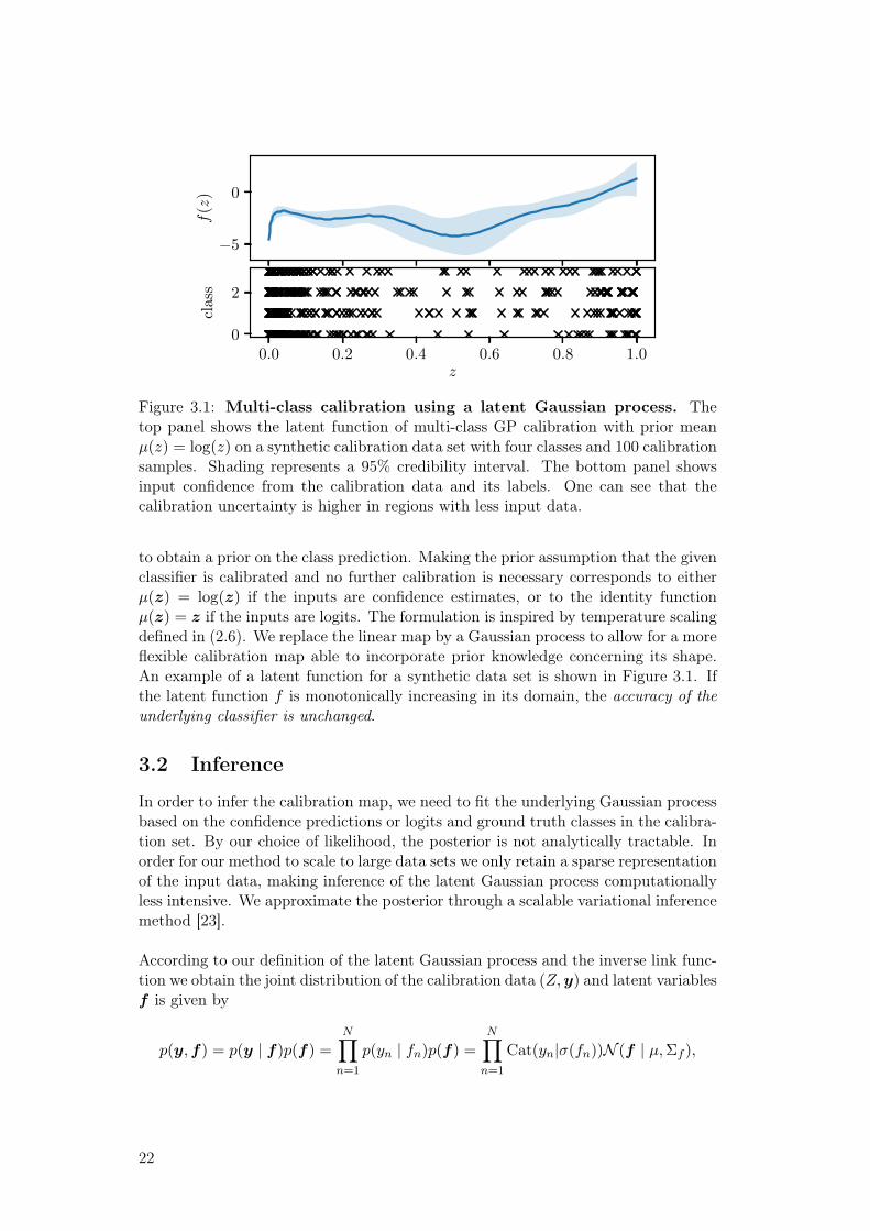
3.1 Multi-class calibration using a latent Gaussian process. Thetop panel shows the latent function of multi-class GP calibration withprior mean µ(z) = log(z) on a synthetic calibration data set withfour classes and 100 calibration samples. Shading represents a 95%credibility interval. The bottom panel shows input confidence fromthe calibration data and its labels. One can see that the calibrationuncertainty is higher in regions with less input data. . . . . . . . . . 22

3.2 Taylor approximation of the log-softargmax function. Illustra-tion of the second-order Taylor approximation to the log-softargmaxfunction (3.10) for a binary calibration problem with y = 0 and meanof the variational distribution ϕn = (0, 0)>. . . . . . . . . . . . . . . 25

4.1 Traffic scene from the KITTI data set. Still image captured froman example sequence of the KITTI data set [60] showing point cloudsin white on black background, ground truth bounding boxes in colorand a road overlay. The image at the top shows the camera imagerecorded by the stereo camera system with bounding boxes added. . 30

4.2 Sample scans from the PCam data set. Example images fromthe PCam data set [63] depicting scans of lymph node tissue. Sampleswith metastatic tissue in the center are indicated by green boxes andgiven a positive label. . . . . . . . . . . . . . . . . . . . . . . . . . . 31

4.3 Sample digits from the MNIST data set. Randomly drawnsamples from the MNIST database [19] of handwritten digits. . . . . 31

xiii

4.4 Samples from the ImageNet data set. Illustratory samples fromthe ImageNet data set showing a wide variety of different classes. Dur-ing classification images are rescaled to uniform dimensions. Reprintedfrom [64]. . . . . . . . . . . . . . . . . . . . . . . . . . . . . . . . . . 32

4.5 Reliability diagrams before and after GP calibration. Relia-bility diagrams for synthetic data with 10 classes and a train set with100 data points showing the effect of GP calibration on a test set with900 instances. The uncalibrated reliability diagram is styled after ef-fects often observed in modern network based image classifiers, whichtend to be overconfident. . . . . . . . . . . . . . . . . . . . . . . . . . 34

4.6 Active learning and calibration. ECE1 and classification errorfor two Mondrian forests trained online on labels requested throughan entropy query strategy on the KITTI data set. One Mondrianforest is calibrated at regularly spaced intervals (in gray) using GPcalibration. Raw data and a Gaussian process regression up to theaverage number of queried samples across folds is shown. . . . . . . . 38

4.7 Effects of calibration on over- and underconfidence in ac-tive learning. Over- and underconfidence for two Mondrian foreststrained online in an active fashion. The Mondrian forest which wascalibrated in regularly spaced intervals (in gray) demonstrates a shiftin over- and underconfidence to the ratio determined by Theorem 2.6.Raw data and a Gaussian process regression up to the average numberof queried samples across folds is shown. . . . . . . . . . . . . . . . . 38

xiv

Chapter 1

Introduction

With the recent achievements in machine learning, in particular in the area of deeplearning, the range of applications for learning methods has also increased signifi-cantly. Especially in challenging fields such as computer vision or speech recognition,important advancements have been made using powerful and complex network ar-chitectures, trained on very large data sets. Most of these techniques are used forclassification tasks, e.g. object recognition as illustrated in Figure 1.1. We also con-sider classification in this thesis. However, in addition to achieving high classificationaccuracy, our goal is to also provide reliable uncertainty estimates for predictions.This is of particular relevance in safety-critical applications [1], such as autonomousdriving and robotics. Reliable uncertainties can be used to increase a classifier’s pre-cision by reporting only class labels that are predicted with low uncertainty or forinformation theoretic analyses of what was learned and what was not. The latter isespecially interesting in the context of active learning [2], where the learner activelyselects the most relevant data samples for training via a query function based on theposterior predictive uncertainty of the model.

Unfortunately, current probabilistic classification approaches that inherently providegood uncertainty estimates, such as Gaussian processes, often suffer from a loweraccuracy and a higher computational complexity on high-dimensional classificationtasks compared to state-of-the-art convolutional neural network (CNN) architec-tures. It was recently observed that many modern CNNs are overconfident [4] andmiscalibrated [5]. Here, calibration refers to adapting the confidence output of aclassifier such that it matches its true probability of being correct. Originally devel-oped in the context of forecasting [6, 7], probability calibration has seen increasedinterest in recent years [5, 8–11], partly because of the popularity of CNNs whichlack inherent uncertainty representation. Earlier studies show that also classicalmethods such as decision trees, boosting, SVMs and naive Bayes classifiers tendto be miscalibrated [8, 12–14]. Therefore, we claim that training and calibrating aclassifier can be two different objectives that need to be considered separately, asexemplified in a toy example in Figure 1.2. Here, a simple neural network contin-ually improves its accuracy on the test set during training, but eventually overfitsin terms of NLL and calibration error. A similar phenomenon was observed in [5]for more complex models. Calibration methods perform a post-hoc improvement to

1

Figure 1.1: Example classification task in autonomous driving. Segmentedscenery of Tübingen from the cityscapes data set [3] with a bounding box aroundan object, demonstrating an example classification task for an autonomous car.

uncertainty estimation using a small subset of the training data. In this thesis wedevelop a multi-class calibration method for arbitrary classifiers, to provide reliablepredictive uncertainty estimates in addition to maintaining high accuracy.

We note that in contrast to recent approaches which strive to improve uncertaintyestimation only for neural networks, including Bayesian neural networks [15, 16] andLaplace approximations (LA) [17, 18], our aim is a framework that is not based ontuning a specific classification method. This has the advantage that the methodoperates independently of the training process of the classifier and does not rely ontraining-specific values such as the curvature of the loss function as in LA methods.

1.1 Research Question and Contribution

The research question which will be examined in this thesis is the following. How canprediction uncertainty of a multi-class classifier, applied to computer vision prob-lems, be accurately represented independent of model specification? We made thefollowing contributions in this thesis in an attempt to answer this question.

We show a theoretical link between calibration, over- and underconfidence, con-necting these formerly disparate concepts. Further, we demonstrate on a range ofclassification models and benchmark data sets that popular classification modelsare often not calibrated. The main contribution of this thesis is a new multi-classand model-agnostic approach to calibration, based on Gaussian processes. Finally,we study the relationship between active learning and calibration from a theoreticaland empirical perspective.

2

0 20 40 60

epoch

0.00

0.05

error

0 20 40 60

epoch

0.0

0.2

NLL

0 20 40 60

epoch

0.02

0.04

ECE1

traintesttest + calibr.

Figure 1.2: Motivating example for calibration. We trained a neural networkwith one hidden layer on MNIST [19] and computed the classification error, the neg-ative log-likelihood (NLL) and the expected calibration error (ECE1) over trainingepochs. We observe that while accuracy continues to improve on the test set, theECE1 increases after 20 epochs. Note that this is different from classical overfitting,as the test error continues to decrease. This shows that training and calibrationneed to be considered independently. This can be mitigated by post-hoc calibrationusing our method (dashed red line). The uncertainty estimation is improved withmaintained classification accuracy.

1.2 Related Work

Estimation of uncertainty is of considerable interest in the machine learning com-munity at the moment. There are two main approaches in classification. First, bydefining a model and loss function which inherently learns a good representation andsecond, by post-hoc calibration methods which transform output of the underlyingmodel. Uncertainty estimation is also connected to adversarial robustness. Theo-retical results on calibration were previously considered in the fairness literature.Finally, calibration in a broader sense is studied in the regression setting and otherapplications. We give a short overview of related work in the following paragraphs.

Uncertainty Estimation for Neural Networks

Uncertainty estimation in deep learning [20] is generally done by some form of reg-ularisation. Pereyra et al. [21] evaluate two output regularizers for deep NNs, amaximum entropy based confidence penalty and label smoothing. They find thatboth improve generalisation on common benchmark data sets. Kumar et al. [10]suggest a trainable measure of calibration as a regulariser in an attempt to improvecalibration during training. Finally, Maddox et al. [22] employ an approximateBayesian inference technique using stochastic weight averaging to obtain an approx-imate posterior distribution over network weights. Bayesian model averaging is thenperformed by sampling from the resulting Gaussian distribution.

Gaussian Processes for Large-Scale Problems

Gaussian processes provide a principled way to represent uncertainty, but generallyperform subpar with regard to accuracy on high-dimensional problems and scalabilityfor very large data sets. Hensman et al. [23] propose a variational inference techniqueto scale Gaussian processes to large data sets and perform inference for intractablelikelihoods. Milios et al. [24] approximate Gaussian process classifiers, which tend to

3

have good uncertainty estimates by GP regression on transformed labels for improvedscalability.

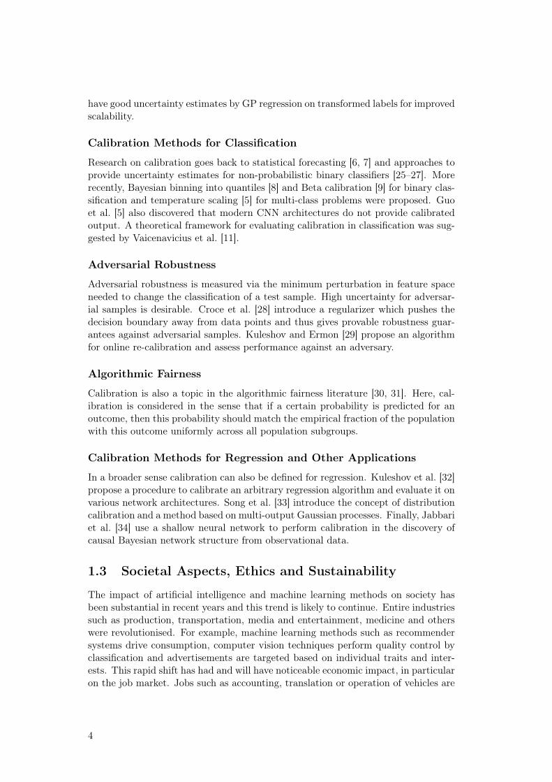
Calibration Methods for Classification

Research on calibration goes back to statistical forecasting [6, 7] and approaches toprovide uncertainty estimates for non-probabilistic binary classifiers [25–27]. Morerecently, Bayesian binning into quantiles [8] and Beta calibration [9] for binary clas-sification and temperature scaling [5] for multi-class problems were proposed. Guoet al. [5] also discovered that modern CNN architectures do not provide calibratedoutput. A theoretical framework for evaluating calibration in classification was sug-gested by Vaicenavicius et al. [11].

Adversarial Robustness

Adversarial robustness is measured via the minimum perturbation in feature spaceneeded to change the classification of a test sample. High uncertainty for adversar-ial samples is desirable. Croce et al. [28] introduce a regularizer which pushes thedecision boundary away from data points and thus gives provable robustness guar-antees against adversarial samples. Kuleshov and Ermon [29] propose an algorithmfor online re-calibration and assess performance against an adversary.

Algorithmic Fairness

Calibration is also a topic in the algorithmic fairness literature [30, 31]. Here, cal-ibration is considered in the sense that if a certain probability is predicted for anoutcome, then this probability should match the empirical fraction of the populationwith this outcome uniformly across all population subgroups.

Calibration Methods for Regression and Other Applications

In a broader sense calibration can also be defined for regression. Kuleshov et al. [32]propose a procedure to calibrate an arbitrary regression algorithm and evaluate it onvarious network architectures. Song et al. [33] introduce the concept of distributioncalibration and a method based on multi-output Gaussian processes. Finally, Jabbariet al. [34] use a shallow neural network to perform calibration in the discovery ofcausal Bayesian network structure from observational data.

1.3 Societal Aspects, Ethics and Sustainability

The impact of artificial intelligence and machine learning methods on society hasbeen substantial in recent years and this trend is likely to continue. Entire industriessuch as production, transportation, media and entertainment, medicine and otherswere revolutionised. For example, machine learning methods such as recommendersystems drive consumption, computer vision techniques perform quality control byclassification and advertisements are targeted based on individual traits and inter-ests. This rapid shift has had and will have noticeable economic impact, in particularon the job market. Jobs such as accounting, translation or operation of vehicles are

4

likely to be replaced by automated systems in the future [35]. Widespread use ofartificial intelligence also raises many questions regarding ethics, privacy, fairnessand environmental impact.

One area which has been impacted heavily by automated statistical analysis is pri-vacy. It is routine business practice of social media companies to use personalisedadvertising as the main stream of revenue. This relies on building a statistical modelof consumer behaviour, based on their interaction data with the specific site. It isvery important to protect an individual’s right to privacy, in particular since manyusers of such a website are not aware of how their data is being used. These changesrequire careful analysis and possible regulatory action to protect the consumer [36].One area where privacy is particularly crucial is facial recognition. Such technologiescan be easily misused by organisations or governments to control and monitor.

The routine reliance on data in order to make decisions and the apparent objectiv-ity of statistical models can introduce unwanted bias. Fairness, the concept thatsubgroups of a population are treated equally in a model should be considered in or-der to avoid discrimination. There are many examples of systems like credit scoresand crime risk being heavily skewed towards economically disadvantaged popula-tion groups or minorities [37], job platforms ranking people based on qualificationshave been found to disproportionally undervalue women [38] and facial recognitionsoftware, trained predominantly on light skinned faces, fails when presented with ahuman face with darker complexion [39]. These examples underline the challengeswhen relying on automated systems learning from data and their ethical impact.

Computing also has a considerable environmental impact [40]. Many components ofmodern computers use rare materials which are extracted and manufactured underdangerous conditions, often in economically disadvantaged nations with low wagelevels. Further computing in general and training large scale machine learning mod-els in particular has significant energy cost (e.g. Google Deepmind’s AlphaGo [41]).This raises questions of sustainability and the created societal value of a certainapplication with regard to its power usage.

This work specifically touches on many of the general aspects mentioned above. Allbenchmark data sets for our application are from computer vision, one specificallyfor autonomous driving. It is conceivable that our method could be used in facialrecognition software at some point in the future. Further, our approach which wewill outline later in this thesis is not robust against biased data and thus its use mayraise questions of fairness. The main societal relevance of our thesis is in improv-ing classification systems. As mentioned above automated statistical classificationis ubiquitous in modern society. By improving uncertainty representation in suchmethods we aim to make automated systems safer, easier to use and interpret andfaster to improve. This work has a theoretical and research focus and is thus targetedtowards the research community.

5

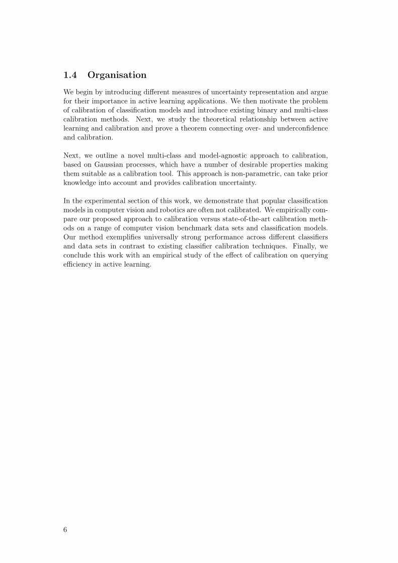
1.4 Organisation

We begin by introducing different measures of uncertainty representation and arguefor their importance in active learning applications. We then motivate the problemof calibration of classification models and introduce existing binary and multi-classcalibration methods. Next, we study the theoretical relationship between activelearning and calibration and prove a theorem connecting over- and underconfidenceand calibration.

Next, we outline a novel multi-class and model-agnostic approach to calibration,based on Gaussian processes, which have a number of desirable properties makingthem suitable as a calibration tool. This approach is non-parametric, can take priorknowledge into account and provides calibration uncertainty.

In the experimental section of this work, we demonstrate that popular classificationmodels in computer vision and robotics are often not calibrated. We empirically com-pare our proposed approach to calibration versus state-of-the-art calibration meth-ods on a range of computer vision benchmark data sets and classification models.Our method exemplifies universally strong performance across different classifiersand data sets in contrast to existing classifier calibration techniques. Finally, weconclude this work with an empirical study of the effect of calibration on queryingefficiency in active learning.

6

Chapter 2

Background

Suppose we are trying to learn the relationship between a set of inputs x and outputsy with the goal of predicting the output of unseen inputs. For example, we might beinterested in predicting the classes of objects visible in an image in order to decidewhether a robot can interact with them safely. If y takes on a discrete set of valuesor classes, we call this problem classification. This problem falls under the broadercategory of supervised learning, meaning we have access to a set of training dataD = (xn, yn)Nn=1 of examples of the relationship between inputs and outputs. Morerigorously, we can formulate this problem as a form of function approximation, whereinputs and outputs come from an underlying distribution which we are trying touncover. Out of the many introductory texts on supervised learning and classificationwhich exist, we relied mostly on [42–44] for this introduction. Taking a probabilisticview, we define the problem formally below.

2.1 Classification

Let X be a vector space and Y a set of finite cardinality K = |Y|. Further, let(Ω,F , P ) be a probability space and X : Ω → X , Y : Ω → Y random variables onsaid space. We assume we have access to a training data set D of independent andidentically distributed samples from (X,Y ) of size N . The relationship between Xand Y is fully determined by its joint density function fX,Y : X × Y → R.

Modeling the relationship between X and Y comes down to approximating theirjoint density function. We call a function f : X × Y → R a classifier or model andy = arg maxy∈Y f(x, y) for some x ∈ X its class prediction. We will abuse notationand sometimes use f : X → RK with output z = f(x), prediction y = arg maxi(zi)and associated confidence score z = maxi(zi) instead. Modeling the relationshipdefined by fX,Y can be approached in two ways, according to Ng and Jordan [45].One can either take a generative approach and model the joint distribution p(x, y),or a discriminative approach and model the posterior p(y | x) directly, i.e. learna mapping from inputs x to outputs y. These two approaches are illustrated inFigure 2.1.

In order to decide between classifiers a loss function L(f,D) is used. It scores a

7

(a) Discriminative model (b) Generative model

Figure 2.1: Illustration of the two approaches to modelling in classification.One can take one of two approaches when trying to model the latent relationshipbetween inputs and outputs in the training data. Either one takes a discriminativeapproach, modelling the posterior fX,Y (y | x) directly or a generative approachmodelling the joint distribution fX,Y (x, y). Reprinted from [46].

Table 2.1: Examples of common loss functions used in classification. Lossfunctions allow the comparison of different classification models by scoring themusing samples from (X,Y ). We list a few common loss functions for a single input -output pair (x, y).

Loss function Definition

0/1 loss 1y 6=ySquared loss (1− yf(x))2

Exponential loss exp(−αyf(x))Hinge loss max(0, 1− yf(x))

Log loss (Cross entropy) −y+12 log(f(x))− (1− y+1

2 ) log(1− f(x))

classifier by comparing the predictions and associated confidence scores of the clas-sifier on a set of inputs with the true outputs or labels. Some common examples ofloss functions are presented in Table 2.1. As the space of all possible functions istoo vast to be useful, one restricts the class of functions which model the relation-ship defined by fX,Y . This modelling task is where knowledge about the applicationwhere the data is coming from is essential. For example, sometimes a mechanisticunderstanding about a physical system is available or some rules about what typeof data is classified into which class is known a priori. During training one uses thetraining data to compute the loss for a set of models from the chosen class to choosethe best fitting one.

Often one also introduces a regularisation term R(f) which penalises functions fromthe chosen class in different ways. This can be useful to combat overfitting, the phe-nomenon of modelling the training data too well, resulting in a lack of generalisation,i.e. small loss on the training data but large loss on independent data sampled from(X,Y ).

8

2.2 Uncertainty Representation

In this work we are particularly interested in uncertainty representation, i.e. howwell a classifier is aware of what it does not know. This is important because in ap-plications it is often not sufficient to have high accuracy on a classification task. Forexample consider an autonomous robot which is deployed in a novel environment,such as a remote planet or a city destroyed by an earthquake. During navigationthis robot has to make choices continuously of what type of objects are in its pathand whether it is safe to interact with them. Some of these classifications can besafety-critical for example whether to drive over a ledge or to interact with a po-tential disaster victim. Proper uncertainty about its prediction allows the robot torefrain from making potentially dangerous decisions. For example when the robothas high uncertainty on whether it is safe to drive to a certain location, it can firstask for feedback on its camera image from a human supervisor on earth, before tak-ing action. It could also record high uncertainty predictions in order to obtain thetrue classification at a later date from an expert in order to improve its predictionsin the future. This type of learning strategy is called active learning by uncertaintysampling.

We are interested in correctly modelling predictive uncertainty, the posterior proba-bility of the class prediction fX,Y (y | x) or if viewed from the classifier perspective,the uncertainty a classifier has about its prediction. One can further split the pre-dictive uncertainty into at least two types [16]. Epistemic uncertainty or modeluncertainty is caused by uncertainty about the correct parameters and structure ofthe underlying model and aleatoric uncertainty or uncertainty caused by inherentnoise in the training data.

2.3 Measures of Uncertainty Representation

So far we have not defined what it means to have good uncertainty representation.This is due to the fact that this comes down to the modelling choices made and canvary for different applications. One usually tries to measure how close the model fis to the true data distribution fX,Y . This can be done in different ways. One candefine a metric on a space of probability measures (e.g. Wasserstein metric), one canmeasure the distance between probability distributions (e.g. KL divergence) if thetrue data distribution is known, or one can represent a probability distribution as anelement of a reproducing kernel Hilbert space (e.g. maximum mean discrepancy).Typically these distances rely on samples from one or both distributions as fX,Yis usually unknown. Focussing on uncertainty representation means putting valueon closeness with respect to the chosen statistical distance and not only on accuracy.

In the following, we will introduce a set of measures used to quantify uncertaintyrepresentation. We are particularly interested in the concept of calibration, thenotion that a classifier’s uncertainty in its prediction matches its empirical accuracy.

9

In practice, we evaluate these measures on a test data set, which we assume toconsist of i.i.d. samples from the ground truth distribution.

2.3.1 Negative Log-Likelihood and Cross Entropy

We begin by defining cross entropy, an information-theoretic quantity which can beused to compare probability distributions and is commonly used as a loss functionfor example in logistic regression.

Definition 2.1Let f(y | x) be a model approximating the conditional distribution of the data.We define the cross entropy as

H(fY |X , f) = EX,Y [− log f ] . (2.1)

Remark 2.2The following identity for the cross entropy holds

EX,Y [− log f ] = H(fY |X) + KL[fY |X ||f ],

where H is the information-theoretic entropy and KL[fY |X ||f ] the Kullback-Leibler divergence. Since KL[·||·] ≥ 0, we see that the ground truth distributionminimises the cross entropy.

Cross-entropy in the context of machine learning is closely related to maximum like-lihood estimation. When fitting a family of parametric statistical models, maximumlikelihood estimation (MLE) is used to identify the value of the parameter, for whichthe probability of the observed sample is maximised. Due to the monotonicity ofthe natural logarithm we can equivalently minimise the negative log-likelihood. Infact, when evaluating the negative log-likelihood on an i.i.d. sample from (X,Y ), itis given by

L = −n∑i=1

log f(yi | xi),

which can be seen as a Monte-Carlo estimator of 2.1.

2.3.2 Calibration and Sharpness

Originally introduced in the context of statistical forecasting [6, 7] calibration de-scribes how well the confidence of a classifier in its prediction matches the empiricalfrequency of its prediction being correct.

Definition 2.3Let f be a model, y its class prediction and z the associated confidence score.A classifier is called calibrated if

P (y = y | z = z) = z ∀z ∈ [0, 1],

10

or equivalentlyE [1y=y | z] = z. (2.2)

In order to measure degree of calibration, we define the expected calibrationerror [8] for 1 ≤ p <∞ by

ECEp = E [|z − E [1y=y | z]|p]1p (2.3)

and the maximum calibration error [8] by

ECE∞ = maxz∈[0,1]

|z − E [1y=y | z = z]|. (2.4)

In practice, we estimate the calibration error as suggested by Naeini et al. [8] byintroducing a fixed binning θ0 < θ1 < · · · < θB such that

ECEp ≈1

B

(B∑b=1

∣∣¯zb − accb∣∣) 1

p

,

where¯zb =

1

Nb

∑θb−1<z≤θb

z

is the mean confidence,

accb =1

Nb

∑θb−1<z≤θb

1y=y

the accuracy and Nb the number of samples in bin b.

Calibration on its own is not a sufficient criterium for confidence estimates of aclassifier to be meaningful. In a two-class problem with equal prior probabilityfor both classes, a classifier which chooses either of the two classes at random withprobability 0.5 is calibrated. However it is immediately apparent that such a classifieris of little use. Intuitively, for a classifier’s confidence estimates to be meaningful,they need to be sufficiently close to 0 or 1, at least some of the time.

Definition 2.4We define the sharpness of f by

sharp(f) =4k2

(k − 1)2Var [z] ∈ [0, 1]. (2.5)

The sharpness represents the scaled variance of the confidence in the predicted class.It is scaled such that it is always in the unit interval no matter the number of classesof the problem. Sharpness has been defined in various ways in previous works, re-flecting the fact that there are a multitude of measures of concentration for a randomvariable. Variations of this notion are also known as refinement [7, 47, 48].

11

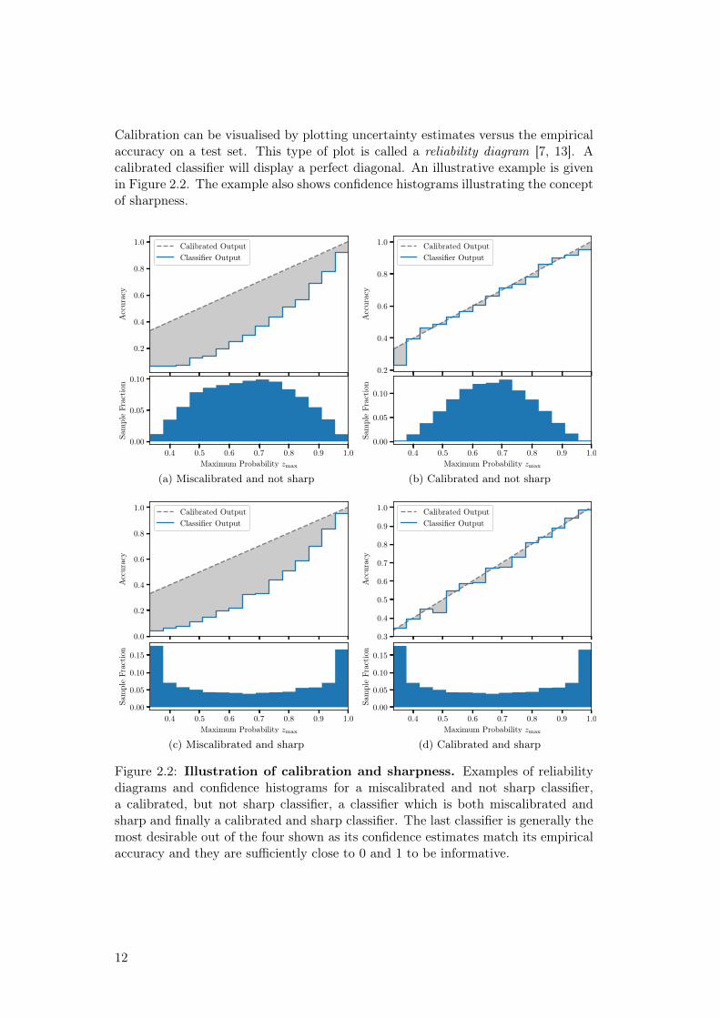
Calibration can be visualised by plotting uncertainty estimates versus the empiricalaccuracy on a test set. This type of plot is called a reliability diagram [7, 13]. Acalibrated classifier will display a perfect diagonal. An illustrative example is givenin Figure 2.2. The example also shows confidence histograms illustrating the conceptof sharpness.

0.2

0.4

0.6

0.8

1.0

Accuracy

Calibrated OutputClassifier Output

0.4 0.5 0.6 0.7 0.8 0.9 1.0

Maximum Probability zmax

0.00

0.05

0.10

SampleFraction

(a) Miscalibrated and not sharp

0.2

0.4

0.6

0.8

1.0

Accuracy

Calibrated OutputClassifier Output

0.4 0.5 0.6 0.7 0.8 0.9 1.0

Maximum Probability zmax

0.00

0.05

0.10

SampleFraction

(b) Calibrated and not sharp

0.0

0.2

0.4

0.6

0.8

1.0

Accuracy

Calibrated OutputClassifier Output

0.4 0.5 0.6 0.7 0.8 0.9 1.0

Maximum Probability zmax

0.00

0.05

0.10

0.15

SampleFraction

(c) Miscalibrated and sharp

0.3

0.4

0.5

0.6

0.7

0.8

0.9

1.0

Accuracy

Calibrated OutputClassifier Output

0.4 0.5 0.6 0.7 0.8 0.9 1.0

Maximum Probability zmax

0.00

0.05

0.10

0.15

SampleFraction

(d) Calibrated and sharp

Figure 2.2: Illustration of calibration and sharpness. Examples of reliabilitydiagrams and confidence histograms for a miscalibrated and not sharp classifier,a calibrated, but not sharp classifier, a classifier which is both miscalibrated andsharp and finally a calibrated and sharp classifier. The last classifier is generally themost desirable out of the four shown as its confidence estimates match its empiricalaccuracy and they are sufficiently close to 0 and 1 to be informative.

12

2.3.3 Over- and Underconfidence

In the context of active learning, where only the most informative data is queriedfor labels, an accurate representation of uncertainty is important in order for theclassifier to obtain informative samples. Informative samples are those that improvethe classifier’s accuracy on future data. In particular, obtaining more samples inregions of the input space, which are misclassified with the current model and lessfor regions which the classifier already predicts correctly as these are uninformativeis desirable. Over- and underconfidence, introduced in [49] capture this notion.

Definition 2.5Let z ∈ [0, 1] be the confidence score output by a model f at x. We define theoverconfidence of f as the expected confidence on the misclassified samples

o(f) = E [z | y 6= y]

and analogously underconfidence as the average uncertainty on the correctlyclassified samples

u(f) = E [1− z | y = y] .

Overconfidence measures the average confidence a classifier has in the samples it clas-sifies wrongly. When using an uncertainty sampling based strategy in active learning,this means that wrongly classified samples are rarely requested as the classifier hashigh confidence in its prediction for them. The flip-side of this is underconfidence.It describes the average uncertainty of the classifier about its correctly classifiedsamples. If a classifier has high underconfidence it queries many samples which italready classifies correctly, i.e. predominantly uninformative samples. Ideally bothover- and underconfidence are low. It is also important to note that both quantitiesare by definition independent of accuracy.

In [49] these notions of introspective capability of a classifier were used to improveuncertainty sampling in the context of active learning. They introduced a variantof a gradient boosting algorithm which weighted those samples more which werewrongly classified with high confidence. Figure 2.3 shows how this strategy improvedaccuracy compared to regular gradient boosting and lowered the number of queriedlabels.

2.4 Calibration Methods

Calibration methods were originally developed to provide probabilistic output fordiscriminative models such as support vector machines (SVMs). They were lateradapted to be used as post-hoc methods to improve uncertainty representation bylowering calibration error. They work by using a small subset of the training dataand subsequently adjusting the confidence output of the underlying model. A dia-grammatic explanation of calibration is shown in Figure 2.4. Figure 2.5 illustratesthe effect of calibration in a binary classification problem on prediction uncertainty.

13

(a) Learning curves of passive and activegradient and confidence boosting on thePenDigits data set.

(b) Number of new label queries perepoch on different data sets.

Figure 2.3: Effect of confidence boosting in active learning. Comparison ofgradient and confidence boosting on various data sets with respect to accuracy andquerying efficiency. Panel (a) shows learning curves for active and passive gradientand confidence boosting on the PenDigits data set. Gradient boosting displaysbetter accuracy for less queried labels. Panel (b) compares the number of queriesper learning epoch of gradient versus confidence boosting on different data sets.Figure reprinted from [49].

Calibration has seen a resurgence of interest in recent years, partly due to the pop-ularity of large neural network architectures and their lack of calibration [5] evenwhen combined with principled Bayesian approaches [50]. An example of this isshown in Figure 2.6. In this section, we introduce the most prevalent methods.

2.4.1 Binary Calibration

We begin by introducing common binary calibration methods. We denote a binarycalibration method by v : R→ R. It transforms the confidence for the positive classz1 and then computes the calibrated confidence for the negative class by 1− v(z1).

Platt scaling Originally introduced in the context of SVMs, Platt Scaling [25,26] is a parametric method designed to output calibrated posterior probabilities fornon-probabilistic binary classifiers. It works by fitting a logistic regression model tothe model output using the negative log-likelihood as a loss function. Let z1 ∈ R bethe output of a model. The probabilistic score computed via Platt scaling is definedas

v(z1) =1

1 + exp(−az1 − b),

where a, b ∈ R are the parameters determined in the fitting procedure. The para-metric assumption made corresponds to the case where the scores of each class arenormally distributed with identical variance across classes [51].

Isotonic Regression Isotonic regression [27] is a non-parametric approach tomapping non-probabilistic classifier scores to probabilities. It relaxes the assumption

14

training data Classifier

CalibrationMethod

new data

prediction

calib

ratio

n da

ta

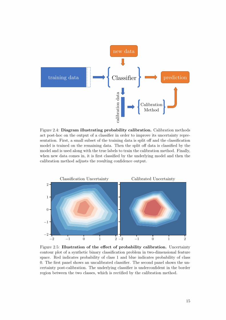
Figure 2.4: Diagram illustrating probability calibration. Calibration methodsact post-hoc on the output of a classifier in order to improve its uncertainty repre-sentation. First, a small subset of the training data is split off and the classificationmodel is trained on the remaining data. Then the split off data is classified by themodel and is used along with the true labels to train the calibration method. Finally,when new data comes in, it is first classified by the underlying model and then thecalibration method adjusts the resulting confidence output.

−2 −1 0 1 2−2

−1

0

1

2

Classification Uncertainty

−2 −1 0 1 2

Calibrated Uncertainty

Figure 2.5: Illustration of the effect of probability calibration. Uncertaintycontour plot of a synthetic binary classification problem in two-dimensional featurespace. Red indicates probability of class 1 and blue indicates probability of class0. The first panel shows an uncalibrated classifier. The second panel shows the un-certainty post-calibration. The underlying classifier is underconfident in the borderregion between the two classes, which is rectified by the calibration method.

15

of a sigmoidal relationship between the model scores and empirical frequencies madeby Platt scaling to an isotonic (non-decreasing) one. The following model

v(z1) = m(z1) + ε

is assumed for the probabilistic scores. The isotonic function m is found by minimis-ing a squared loss function. In practice, piece-wise constant solutions can be foundby using the pair-adjacent violators (PAV) algorithm [52].

Beta Calibration Specifically designed for probabilistic classifiers with outputrange [0, 1], Beta calibration [9, 51] is a recently introduced parametric approach tocalibration. Here, a calibration map family is defined based on the likelihood ratiobetween two Beta distributions. This parametric assumption is appropriate if themarginal class distributions follow Beta distributions. The model is given by

v(z1) =1

1 + exp(−c) (1−z1)bza1

,

where a, b, c ∈ R are parameters. One theoretical advantage of Beta calibration overPlatt scaling is that it defines a richer family of calibration maps. For example, theidentity map emerges for a = 1, b = 1 and c = 0, which is not part of the sigmoidfamily. When applying Platt scaling to a calibrated classifier, the result will bemiscalibrated.

Histogram Binning Histogram Binning [12] is a straightforward approach tominimising the calibration error. The classifier output range is binned into a fixednumber of bins

0 = θ1 < θ2 < · · · < θB+1 = 1

with thresholds θiB+1i=1 . Then the empirical accuracy in each bin is computed on

the calibration data set giving values aiBi=1. The calibration map is then definedby the piecewise constant map

v(z1) = aj for θj < z1 ≤ θj+1.

The bin edges can be determined for example by equal width or equal frequency.

Bayesian Binning into Quantiles BBQ [8] extends the histogram binning ap-proach in a Bayesian fashion. Here, multiple equal-frequency binning models areconstructed and scored. A binning model M is scored as follows

Score = P (M)P (D |M).

The marginal likelihood P (D | M) can be computed in closed form under the fol-lowing assumptions. All samples are iid and each bin’s class distribution is modelledas a binomial random variable. We assume a Beta(αb, βb) prior on the parameter ofthe binomial distribution in bin b. Then the marginal likelihood is given by

P (D |M) =

B∏b=1

Γ(N′

B )

Γ(Nb + N ′

B )

Γ(mb + αb)

Γ(αb)

Γ(nb + βb)

Γ(βb)

16

where N ′ is the equivalent sample size controlling the influence of the prior, Nb isthe total number of samples in bin b and nb and mb are the number of class 0 andclass 1 instances in bin b respectively. The parameters of the Beta priors are set toαb = N ′

B pb and βb = N ′

B (1 − pb), where pb is the midpoint of bin b. The prior overbinning models P (M) is chosen as uniform. The above score is then used to performmodel averaging across all possible binning models in a given size range.

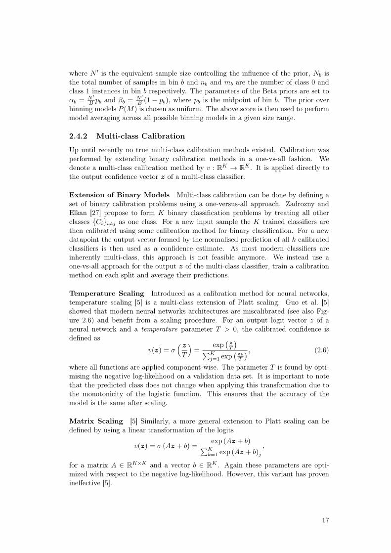
2.4.2 Multi-class Calibration

Up until recently no true multi-class calibration methods existed. Calibration wasperformed by extending binary calibration methods in a one-vs-all fashion. Wedenote a multi-class calibration method by v : RK → RK . It is applied directly tothe output confidence vector z of a multi-class classifier.

Extension of Binary Models Multi-class calibration can be done by defining aset of binary calibration problems using a one-versus-all approach. Zadrozny andElkan [27] propose to form K binary classification problems by treating all otherclasses Cii 6=j as one class. For a new input sample the K trained classifiers arethen calibrated using some calibration method for binary classification. For a newdatapoint the output vector formed by the normalised prediction of all k calibratedclassifiers is then used as a confidence estimate. As most modern classifiers areinherently multi-class, this approach is not feasible anymore. We instead use aone-vs-all approach for the output z of the multi-class classifier, train a calibrationmethod on each split and average their predictions.

Temperature Scaling Introduced as a calibration method for neural networks,temperature scaling [5] is a multi-class extension of Platt scaling. Guo et al. [5]showed that modern neural networks architectures are miscalibrated (see also Fig-ure 2.6) and benefit from a scaling procedure. For an output logit vector z of aneural network and a temperature parameter T > 0, the calibrated confidence isdefined as

v(z) = σ( zT

)=

exp(zT

)∑Kj=1 exp

(zkT

) , (2.6)

where all functions are applied component-wise. The parameter T is found by opti-mising the negative log-likelihood on a validation data set. It is important to notethat the predicted class does not change when applying this transformation due tothe monotonicity of the logistic function. This ensures that the accuracy of themodel is the same after scaling.

Matrix Scaling [5] Similarly, a more general extension to Platt scaling can bedefined by using a linear transformation of the logits

v(z) = σ (Az + b) =exp (Az + b)∑Kk=1 exp (Az + b)j

,

for a matrix A ∈ RK×K and a vector b ∈ RK . Again these parameters are opti-mized with respect to the negative log-likelihood. However, this variant has provenineffective [5].

17

On Calibration of Modern Neural Networks

Chuan Guo * 1 Geoff Pleiss * 1 Yu Sun * 1 Kilian Q. Weinberger 1

AbstractConfidence calibration – the problem of predict-ing probability estimates representative of thetrue correctness likelihood – is important forclassification models in many applications. Wediscover that modern neural networks, unlikethose from a decade ago, are poorly calibrated.Through extensive experiments, we observe thatdepth, width, weight decay, and Batch Normal-ization are important factors influencing calibra-tion. We evaluate the performance of variouspost-processing calibration methods on state-of-the-art architectures with image and documentclassification datasets. Our analysis and exper-iments not only offer insights into neural net-work learning, but also provide a simple andstraightforward recipe for practical settings: onmost datasets, temperature scaling – a single-parameter variant of Platt Scaling – is surpris-ingly effective at calibrating predictions.

1. IntroductionRecent advances in deep learning have dramatically im-proved neural network accuracy (Simonyan & Zisserman,2015; Srivastava et al., 2015; He et al., 2016; Huang et al.,2016; 2017). As a result, neural networks are now entrustedwith making complex decisions in applications, such as ob-ject detection (Girshick, 2015), speech recognition (Han-nun et al., 2014), and medical diagnosis (Caruana et al.,2015). In these settings, neural networks are an essentialcomponent of larger decision making pipelines.

In real-world decision making systems, classification net-works must not only be accurate, but also should indicatewhen they are likely to be incorrect. As an example, con-sider a self-driving car that uses a neural network to detectpedestrians and other obstructions (Bojarski et al., 2016).

*Equal contribution, alphabetical order. 1Cornell University.Correspondence to: Chuan Guo <cg563@cornell.edu>, GeoffPleiss <geoff@cs.cornell.edu>, Yu Sun <ys646@cornell.edu>.

Proceedings of the 34 th International Conference on MachineLearning, Sydney, Australia, PMLR 70, 2017. Copyright 2017by the author(s).

0.0 0.2 0.4 0.6 0.8 1.00.0

0.2

0.4

0.6

0.8

1.0

%of

Sam

ples

Avg

.con

fiden

ceA

ccur

acy

LeNet (1998)CIFAR-100

0.0 0.2 0.4 0.6 0.8 1.0

Avg

.con

fiden

ce

Acc

urac

y

ResNet (2016)CIFAR-100

0.0 0.2 0.4 0.6 0.8 1.00.0

0.2

0.4

0.6

0.8

1.0

Acc

urac

y

Error=44.9

OutputsGap

0.0 0.2 0.4 0.6 0.8 1.0

Error=30.6

OutputsGap

Confidence

Figure 1. Confidence histograms (top) and reliability diagrams(bottom) for a 5-layer LeNet (left) and a 110-layer ResNet (right)on CIFAR-100. Refer to the text below for detailed illustration.

If the detection network is not able to confidently predictthe presence or absence of immediate obstructions, the carshould rely more on the output of other sensors for braking.Alternatively, in automated health care, control should bepassed on to human doctors when the confidence of a dis-ease diagnosis network is low (Jiang et al., 2012). Specif-ically, a network should provide a calibrated confidencemeasure in addition to its prediction. In other words, theprobability associated with the predicted class label shouldreflect its ground truth correctness likelihood.

Calibrated confidence estimates are also important formodel interpretability. Humans have a natural cognitive in-tuition for probabilities (Cosmides & Tooby, 1996). Goodconfidence estimates provide a valuable extra bit of infor-mation to establish trustworthiness with the user – espe-cially for neural networks, whose classification decisionsare often difficult to interpret. Further, good probabilityestimates can be used to incorporate neural networks intoother probabilistic models. For example, one can improveperformance by combining network outputs with a lan-

Figure 2.6: Modern NN architectures are miscalibrated. Confidence his-tograms (top) and reliability diagrams (bottom) of a simple and a modern neuralnetwork architecture’s confidence estimates on the CIFAR-100 data set [53]. Themodern neural network displays lower error but is more overconfident and thus lesscalibrated. Graphs reprinted from [5].

2.5 Relations between Measures of Uncertainty Repre-sentation

While the importance of different measures of uncertainty quantification is applica-tion specific, many of them are inherently linked. Here we will study more closelyhow calibration, over- and underconfidence and sharpness are linked.

2.5.1 Calibration, Over- and Underconfidence

Since over- and underconfidence are properties independent of accuracy, they seemto be at first glance also independent of calibration, a property defined through clas-sification accuracy. But as it turns out there is a quite important connection. Thecloser a classifier is to being calibrated, the closer the ratio between its over- under-confidence is determined by the odds of the classifier making a correct prediction.

Theorem 2.6Let 1 ≤ p < q ≤ ∞, then the following relationship between over-, underconfi-dence and the expected calibration error holds:

|o(f)P(y 6= y)− u(f)P(y = y)| ≤ ECEp ≤ ECEq (2.7)

18

Proof. By linearity and the law of total expectation it holds that

E [z] = E [z + E [1y=y | z]− E [1y=y | z]] = E [z − E [1y=y | z]] + P(y = y).

Conversely, by decomposing the average confidence we have

E [z] = E [z | y 6= y]P(y 6= y) + E [z | y = y]P(y = y)

= E [z | y 6= y]P(y 6= y) + (1− E [1− z | y = y])P (y = y)

= o(f)P(y 6= y) + (1− u(f))P(y = y).

Combining the above we obtain

E [z − E [1y=y | z]] = o(f)P(y 6= y)− u(f)P(y = y).

Now, since f(x) = |x|p is convex for 1 ≤ p <∞, we have by Jensen’s inequality

|E [z − E [1y=y | z]]|p ≤ E [|z − E [1y=y | z]|p]

and finally by Hölder’s inequality with 1 ≤ p < q ≤ ∞ it follows that

ECEp = E [|z − E [1y=y | z]|p]1p ≤ E [|z − E [1y=y | z]|q]

1q = ECEq,

which concludes the proof.

While a similar result for ECE1 was shown in the context of fairness in [30] fordifferent population groups in X , the sharpness of the bound and the generalisationto 1 ≤ p < q ≤ ∞ are original results to the best of our knowledge.

Corollary 2.7Assume f is calibrated, then

o(f)P(y 6= y) = u(f)P(y = y), (2.8)

i.e. the odds of making a correct prediction determine the ratio between over-and underconfidence. Assuming P(y 6= y) /∈ 0, 1 we obtain

o(f)

u(f)=

P(y = y)

P(y 6= y).

Proof. Since f is calibrated we have by definition

ECEp = E [|z − E [1y=y | z]|p]1p = 0,

i.e. the calibration gap is zero. By Theorem 2.6 we have

o(f)P(y 6= y)− u(f)P(y = y) = 0.

Rearranging terms concludes the proof.

The relationship described in Theorem 2.7 was previously established in the fairnessliterature by [30, 31]. The authors show that for each population group the aboveholds under separate calibration of each group.

19

2.5.2 Sharpness, Over- and Underconfidence

While the previous subsection established a relationship between calibration andover- and underconfidence it does not yet provide us with a way to minimise them.A fixed ratio of the two can still imply both to be high. Here we will establish howsharpness influences over- and underconfidence. Intuitively a sharp classifier makeseither very confident or very uncertain predictions. If the classifier is calibrated thesehave high and low accuracy respectively. The definition of over- and underconfidencethen suggests that increased sharpness under calibration should reduce both. Thissubsection formalises this heuristic argument.

Proposition 2.8The following relationship between sharpness and over- / underconfidence of fholds:

sharp(f) =4k2

(k − 1)2(P (y 6= y)

(Var [z | y 6= y] + (o(f)− E [z])2

)+ P (y = y)

(Var [1− z | y = y] + (u(f)− E [1− z])2

))

(2.9)

Proof. Using the law of total variance, we obtain

Var [z] = E [Var [z | 1y=y]] + Var [E [z | 1y=y]]= E

[Var [z | 1y=y] + (E [z | 1y=y]− E [E [z | 1y=y]])2

]= P(y 6= y)

(Var [z | y 6= y] + (E [z | y 6= y]− E [z])2

)+ P(y = y)

(Var [z | y = y] + (E [z | y = y]− E [z])2

)= P(y 6= y)

(Var [z | y 6= y] + (E [z | y 6= y]− E [z])2

)+ P(y = y)

(Var [1− z | y = y] + (E [z | y = y]− 1 + 1− E [z])2

)= P(y 6= y)

(Var [z | y 6= y] + (o(f)− E [z])2

)+ P(y = y)

(Var [1− z | y = y] + (u(f)− E [1− z])2

).

Now the result follows directly from the definition of sharpness.

The combination of Theorem 2.7 and Theorem 2.8 imply that for a calibrated clas-sifier for which one of the regularity conditions

o(f) ≤ E [z] or u(f) ≤ E [1− z]

holds, a sufficient increase in sharpness of f decreases both over- and underconfidenceas long as the individual variances can be controlled. In the rest of this thesis we willfocus solely on improving calibration and leave simultaneous calibration and increasein sharpness based on this theoretical result for future work. We hypothesise thatthe difficulty lies in calibration and controlling the variance terms simultaneously.

20

Chapter 3

Gaussian Process Calibration

We outline our non-parametric calibration method in the following sections. Ouraim is to develop a calibration algorithm, which is inherently multi-class, suitable forarbitrary classifiers, makes no parametric assumption on the shape of the calibrationmap and can take prior knowledge into account. These desired properties readilylead to our approach using a latent Gaussian process [54]. This has the addedbenefit that we obtain calibration uncertainty providing us with information abouthow much we can trust the calibration map in different regions of its input space.

3.1 Definition

Assume a one-dimensional Gaussian process prior over the latent function f(z), i.e.

f ∼ GP (µ(·), k(· , · | θ))

with mean function µ, kernel k and kernel parameters θ. A common kernel choicemotivated by a smoothness assumption of the calibration map is the squared expo-nential kernel with added noise

k(zi, zj) = σ2 exp

(−(zi − zj)2

2l2

)︸ ︷︷ ︸

squared exponential

+ δijσ2noise.︸ ︷︷ ︸

Gaussian noise

(3.1)

Further, let the calibrated output be given by the softargmax inverse link functionapplied to the latent process evaluated at the model output

v(z)j = σ(f(z))j =exp(f(zj))∑Kk=1 exp(f(zk))

. (3.2)

Note the similarity to multi-class Gaussian process classification, but in contrastwe consider one shared latent function applied to each component of z individuallyinstead of K latent functions. We use the categorical likelihood

Cat(y|σ(f(z))) =

K∏k=1

σ(f(z))[y=k]k (3.3)

21

−5

0f

(z)

0.0 0.2 0.4 0.6 0.8 1.0z

0

2

class

Figure 3.1: Multi-class calibration using a latent Gaussian process. Thetop panel shows the latent function of multi-class GP calibration with prior meanµ(z) = log(z) on a synthetic calibration data set with four classes and 100 calibrationsamples. Shading represents a 95% credibility interval. The bottom panel showsinput confidence from the calibration data and its labels. One can see that thecalibration uncertainty is higher in regions with less input data.

to obtain a prior on the class prediction. Making the prior assumption that the givenclassifier is calibrated and no further calibration is necessary corresponds to eitherµ(z) = log(z) if the inputs are confidence estimates, or to the identity functionµ(z) = z if the inputs are logits. The formulation is inspired by temperature scalingdefined in (2.6). We replace the linear map by a Gaussian process to allow for a moreflexible calibration map able to incorporate prior knowledge concerning its shape.An example of a latent function for a synthetic data set is shown in Figure 3.1. Ifthe latent function f is monotonically increasing in its domain, the accuracy of theunderlying classifier is unchanged.

3.2 Inference

In order to infer the calibration map, we need to fit the underlying Gaussian processbased on the confidence predictions or logits and ground truth classes in the calibra-tion set. By our choice of likelihood, the posterior is not analytically tractable. Inorder for our method to scale to large data sets we only retain a sparse representationof the input data, making inference of the latent Gaussian process computationallyless intensive. We approximate the posterior through a scalable variational inferencemethod [23].

According to our definition of the latent Gaussian process and the inverse link func-tion we obtain the joint distribution of the calibration data (Z,y) and latent variablesf is given by

p(y,f) = p(y | f)p(f) =

N∏n=1

p(yn | fn)p(f) =

N∏n=1

Cat(yn|σ(fn))N (f | µ,Σf ),

22

where y ∈ 1, . . . ,KN , f = (f1, f2, . . . , fN )> ∈ RNK and fn = (f(zn1) . . . , f(znK))> ∈RK . The covariance matrix Σf has block-diagonal structure by independence of thecalibration data, as follows

Σf =

A1,1 · · · 0...

. . ....

0 · · · AN,N

∈ RNK×NK

and each submatrix is given via the kernel function

Ai,j =

k(z1i , z1j | θ) · · · k(z1i , z

Kj | θ)

.... . .

...k(zKi , z

1j | θ) · · · k(zKi , z

Kj | θ)

∈ RK×K ,

where i, j ∈ 1, . . . , N. If performance is critical, a further diagonal assumptioncan be made. This would correspond to the assumption that confidence estimatesfor classes for a given data point are independent. Note that we drop the explicitdependence on Z and θ throughout to lighten the notation.

3.2.1 Inducing Points

Our goal is to compute the posterior p(f | y). In order to reduce the computationalcomplexity from O((NK)3) we focus on inducing point methods. We define Minducing inputs W = (w1, . . . , wM )> ∈ RM and inducing variables u ∈ RM withthe goal to only retain a sparse representation of our Gaussian process at thesepoints. The joint distribution is given by

p(f ,u) = N([fu

] ∣∣∣∣ [µfµu],

[Σf Σf,u

Σ>f,u Σu

]). (3.4)

where the covariance matrix between calibration data and inducing points is givenby

Σf,u =

k(z11 , u1) · · · k(z11 , uM ))

.... . .

...k(zK1 , u1) · · · k(zK1 , uM ))

.... . .

...k(zKN , u1) · · · k(zKN , uM ))

∈ RNK×M

and the covariance matrix at the inducing points by

Σu =

k(u1, u1 | θ) · · · k(u1, uM | θ)...

. . ....

k(uM , u1 | θ) · · · k(uM , uM | θ)

∈ RM×M .

Using Bayes’ theorem and the conditional independence of y and u given f , thejoint can be factorised as

p(y,f ,u) = p(y | f)p(f | u)p(u). (3.5)

23

We aim to find a variational approximation q(u) = N (u|m,S) to the posteriorp(u | y). For general treatments on variational inference we refer interested readersto [55, 56].

3.2.2 Bound on the Marginal Likelihood

We find the variational parameters m and S, the locations of the inducing inputsw and the kernel parameters θ by optimising a lower bound to the marginal log-likelihood log p(y). To begin consider the following bound, derived by marginalisa-tion and Jensen’s inequality

log p(y | u) ≥ Ep(f |u) [log p(y | f)] . (3.6)

We then substitute eq. (3.6) into the lower bound to the evidence (ELBO) as follows

log p(y) = KL [q(u)‖p(u | y)] + ELBO(q(u))

≥ ELBO(q(u))

= Eq(u) [log p(y,u)]− Eq(u) [log q(u)]

= Eq(u) [log p(y | u)]−KL [q(u)‖p(u)]

≥ Eq(u)[Ep(f |u) [log p(y | f)]

]−KL [q(u)‖p(u)]

= Eq(f) [log p(y | f)]−KL [q(u)‖p(u)]

= Eq(f)

[log

N∏n=1

p(yn | fn)

]−KL [q(u)‖p(u)]

=N∑n=1

Eq(fn) [log p(yn | fn)]−KL [q(u)‖p(u)] ,

(3.7)

where the second to last equality holds by independence of the training data and

q(f) :=

∫p(f | u)q(u) du.

By eq. (3.4) and Theorem B.3 we obtain

p(f | u) = N (f | µf + Σf,uΣ−1u (u− µu), Σf − Σf,uΣ−1u Σ>f,u).

With q(u) = N (u | m,S) and A := Σf,uΣ−1u , we have

q(f) :=

∫p(f | u)q(u)︸ ︷︷ ︸

q(f ,u)

du = N (f | µf +A(m− µu), Σf +A(S − Σu)A>). (3.8)

as q(f ,u) is again normally distributed by Theorem B.4 and marginals of multivari-ate normal distributions are normally distributed by Theorem B.1.

24

f 1n

−2.0−1.5 −1.0 −0.5 0.0 0.5 1.0 1.52.0

f2n

−2.0−1.5

−1.0−0.5

0.00.5

1.01.5

2.0

−3.5

−3.0

−2.5

−2.0

−1.5

−1.0

−0.5

0.0

log p(yn | fn)Taylor approx.

Figure 3.2: Taylor approximation of the log-softargmax function. Illustrationof the second-order Taylor approximation to the log-softargmax function (3.10) fora binary calibration problem with y = 0 and mean of the variational distributionϕn = (0, 0)>.

3.2.3 Computation of the Expectation Terms

In order to obtain the variational objective eq. (3.7) we need to compute the expectedvalue terms

Eq(fn) [log p(yn | fn)] = Eq(fn)

[log

exp(fynn )∑Kk=1 exp(fkn)

]

= mynn − Eq(fn)

[log

K∑k=1

exp(fkn

)].

(3.9)

with respect to the K-dimensional marginals of q(f)

q(fn) =

∫p(fn | u)q(u) du = N (fn | ϕn, Cn),

which are normally distributed. To compute the intractable expectation terms (3.9),we use a second order Taylor approximation of

h(fn) := log p(yn | fn) = logexp(fynn )∑Kk=1 exp(fkn)

(3.10)

at fn = ϕn. An illustration is shown in Figure 3.2. We begin by computing theHessian of the log-softargmax. We have

Df log σ(f)y = D2f

[log

exp(fy)∑Kk=1 exp(fk)

]= Df

[fy − log

K∑k=1

exp(fk)

]= ey − σ(f)

25

where ey is the y-th unit vector. Then

D2f log σ(f)y = −

[∂

∂fσ(f)1, . . . ,

∂

∂fσ(f)K

]

= −

σ(f)1(1− σ(f)1) −σ(f)1σ(f)2 · · ·−σ(f)1σ(f)2 σ(f)2(1− σ(f)2) · · ·

.... . .

= σ(f)σ(f)> − diag(σ(f)).

Note, that somewhat surprisingly this expression does not depend on y. Now weobtain by using x>Mx = tr

(x>Mx

), the linearity of the trace and its invariance

under cyclic permutations, that

Eq(fn) [log p(yn | fn)] = Eq(fn) [h(fn)]

≈ Eq(fn)[h(ϕn) +Dfnh(ϕn)>(fn − ϕn) +

1

2(fn − ϕn)>D2

fnh(ϕn)(fn − ϕn)

]= h(ϕn) +

1

2Eq(fn)

[(fn − ϕn)>

(σ(ϕn)σ(ϕn)> − diag(σ(ϕn))

)(fn − ϕn)

]= h(ϕn) +

1

2tr[Eq(fn)

[(fn − ϕn)(fn − ϕn)>

] (σ(ϕn)σ(ϕn)> − diag(σ(ϕn))

)]= log p(yn | ϕn) +

1

2tr[Cn

(σ(ϕn)σ(ϕn)> − diag(σ(ϕn))

)]= log p(yn | ϕn) +

1

2

(tr[σ(ϕn)>Cnσ(ϕn)

]− tr[Cndiag(σ(ϕn))]

)= log p(yn | ϕn) +

1

2

(σ(ϕn)>Cnσ(ϕn)− diag(Cn)>σ(ϕn)

),

which can be computed in O(K2) by expressing the term inside the parenthesesas a double sum over K terms. Computing the KL-divergence term in (3.7) is inO(M3). Therefore, computing the objective (3.7) has complexity O(NK2 + M3).As we assume M N most of the computational expense will be in computing theN expectations. Note that this can be remedied through parallelisation as all Nexpectation terms can be computed independently. Now, the optimisation to findthe variational parameters, the kernel parameters and the inducing point locationscan be performed by using either a gradient-based optimiser or as in our case byautomatic differentiation.

3.3 Prediction

Now that the latent process is fit to the calibration data, we can predict calibrateduncertainties for new input data. Given the approximate posterior

p(f ,u | y) ≈ q(f ,u) := p(f | u)q(u),

26

predictions at new inputs Z∗ are obtained via

p(f∗ | y) =

∫p(f∗ | f ,u)p(f ,u | y) dfdu

≈∫p(f∗ | f ,u)p(f | u)q(u) dfdu

=

∫p(f∗ | u)q(u) du

Note, that p(f∗ | y) is Gaussian by Theorem B.4 as in eq. (3.8). Means and variancesof a latent value f∗ ∈ RK can be computed in O(KM2). The class prediction y∗ isthen obtained by evaluating the integral

p(y∗ | y) =

∫p(y∗ | f∗)p(f∗ | y) df∗

via Monte-Carlo integration. While inference and prediction have higher compu-tational cost than in other calibration methods, it is comparatively small to thetraining time of the underlying classifier, since usually only a small fraction of thedata is necessary for calibration.

3.4 Online Calibration

Streaming sparse Gaussian process approximations [57] could allow for an extensionof our approach to the online setting. This is particularly interesting in active learn-ing applications where we aim to calibrate as data is coming in sequentially.

The comparatively higher computational cost of Gaussian process calibration isremedied in the online setting by three factors. First, calibration is completelyindependent of model training and prediction. Calibration can be done in parallelto online classification and be incorporated once it is completed. In the stream-ing setting fewer samples for calibration can be requested and there is ample timebetween them to calibrate.

3.5 Implementation

All calibration methods from Section 2.4 were implemented using Python 3.6 andare available as a package with documentation at

https://www.github.com/JonathanWenger/pycalib.

An example script demonstrating the use of pycalib is shown in Listing 3.1. Weimplemented the GP calibration’s outlined inference method using gpflow [58], aPython framework for Gaussian process models which builds on tensorflow [59].This allows for automatic differentiation to obtain the gradient of the variationalobjective eq. (3.7) with respect to the variational parameters m and S, the loca-tions of the inducing inputs w and the kernel parameters θ. While these can bederived analytically, automatic differentiation reduces implementation length andcomplexity.

27

Listing 3.1: Code usage example of pycalib. Python code demonstrating onhow to calibrate a random forest classifier on the MNIST data set using Gaussianprocess calibration.1 # Package impo r t s2 impor t numpy as np3 impor t s k l e a r n4 from s k l e a r n . ensemble impor t RandomFo r e s tC l a s s i f i e r5 impor t p y c a l i b . c a l i b r a t i on_method s as calm67 # Seed and data s i z e8 seed = 09 n_test = 1000010 n_ca l i b = 10001112 # Download MNIST data13 X, y = s k l e a r n . d a t a s e t s . fetch_openml ( ’ mnist_784 ’ , v e r s i o n =1,

return_X_y=True , cache=True )14 X = X / 255 .15 y = np . a r r a y ( y , dtype=i n t )1617 # S p l i t data i n t o t r a i n , c a l i b r a t i o n and t e s t18 X_train , X_test , y_tra in , y_test = s k l e a r n . mode l_se l e c t i on .

t r a i n_ t e s t_ s p l i t (X, y , t e s t_ s i z e=n_test , random_state=seed )19 X_train , X_cal ib , y_tra in , y_ca l i b = s k l e a r n . mode l_se l e c t i on .

t r a i n_ t e s t_ s p l i t ( X_train , y_tra in , t e s t_ s i z e=n_cal ib ,

random_state=seed )2021 # Tra in c l a s s i f i e r22 r f = RandomFo r e s tC l a s s i f i e r ( random_state=seed )23 r f . f i t ( X_train , y_t ra in )24 p_uncal = r f . p r ed i c t_proba ( X_test )2526 # Pr e d i c t and c a l i b r a t e output27 gpc = calm . GPCa l i b r a t i o n ( n_c l a s s e s =10, random_state=seed )28 gpc . f i t ( r f . p r ed i c t_proba ( X_cal ib ) , y_ca l i b )29 p_pred = gpc . p r ed i c t_proba ( p_uncal )

28

Chapter 4

Experiments

We experimentally evaluate our approach against the calibration methods presentedin Section 2.4. We use a range of different classifiers on a set of binary and multi-classcomputer vision benchmark data sets and calibrate subsequently. Besides convolu-tional neural networks, we are also interested in ensemble methods such as boostingand forests. These models are still relevant in computer vision and robotics due totheir comparatively smaller computational cost during training and prediction whencompared to large scale neural network architectures.

All methods and experiments were implemented in Python 3.6. We either used theauthors’ original code, if available or re-implemented calibration methods based onthe respective publications. For our GP-based method we used a log mean functionand a sum kernel consisting of an RBF and a white noise kernel as in eq. (3.1). Allexperiments were performed with the implementation described in Section 3.5.

We report the average ECE1 estimated with 100 bins over 10 Monte-Carlo crossvalidation runs. This means we sample a calibration data set without replacementfrom the total data each time. Thus splits may contain the same data points.We choose this cross validation strategy as it allows us to choose the size of thecalibration set and the number of validation splits freely. We used the followingdata sets with indicated train, calibration and test splits:

• KITTI [60, 61]: Stream-based urban traffic scenes with features [62] from seg-mented 3D point clouds. 8 or 2 classes, dimension 60, train: 16000, calibration:1000, test: 8000.

• PCam [63]: Detection of metastatic tissue in histopathologic scans of lymphnode sections converted to gray scale. 2 classes, dimension 96×96, train: 22768,calibration: 1000, test: 9000.

• MNIST [19]: Handwritten digit recognition. 10 classes, dimension 28×28,train: 60000, calibration: 1000, test: 9000.

• ImageNet 2012 [64]: Image database of natural objects and scenes. 1000classes, train: 1.2 million, calibration: 1000, test: 9000.

We give a more detailed explanation of each data set in the following paragraphs.

29

KITTI

The KITTI vision benchmark suite [60] is an autonomous driving data set capturedvia video cameras, a laser scanner and a GPS localisation system. The sensors weremounted on a car driving through various German urban traffic environments. Weuse a version of the data set from the benchmark suite as described in [61], which con-sists of 18 streams of annotated, segmented point clouds, which were concatenatedto one stream. Each feature vector represents points in a bounding box around anobject. Subsequently, a 60-dimensional feature vector is computed via point featurehistograms [62]. These features are particularly suitable to the online setting as theyare computable in real time and low dimensional compared to the original data. Forthe binary setting we group all classes which are no cars into one class. An illustra-tion of the KITTI data set is shown in Figure 4.1. Each of the indicated boundingboxes contains a point cloud which is then converted to a feature representation asdescribed.

Figure 4.1: Traffic scene from the KITTI data set. Still image captured froman example sequence of the KITTI data set [60] showing point clouds in white onblack background, ground truth bounding boxes in color and a road overlay. Theimage at the top shows the camera image recorded by the stereo camera system withbounding boxes added.

PCam

The PatchCamelyon [63] data set consists of 96x96 color images depicting histopatho-logical scans of lymph node tissue. Each image is labelled according to the presenceof metastatic tissue. As medical applications are becoming increasingly important inmachine learning and particularly computer vision, this data set provides a suitablebenchmark. Detection of metastatic tissue is a clinically relevant task and thus mo-tivates the choice of this data set. A subset of the images is shown in Figure 4.2. Inour application we converted the images to gray scale to reduce the dimensionalityof the data set to allow for training of ensemble methods without preceding featureextraction. The color uniformity in the data for different scans justifies this choice.

30

Figure 4.2: Sample scans from the PCam data set. Example images from thePCam data set [63] depicting scans of lymph node tissue. Samples with metastatictissue in the center are indicated by green boxes and given a positive label.

MNIST

The MNIST database [19] of handwritten digits is a commonly used computer visionbenchmark data set containing 70,000 size-normalised and centered 28x28 pixel grayscale images. The images depict handwritten digits 0 through 9 and thus the dataset has 10 classes. Some random samples from the data set are shown in Figure 4.3.

Figure 4.3: Sample digits from the MNIST data set. Randomly drawn samplesfrom the MNIST database [19] of handwritten digits.

ImageNet

ImageNet [64] is an annotated database of more than 14 million images of everydayobjects and scenery classified into over 20,000 different categories. It was publishedas a benchmark vision data set as part of a computer vision research competition.Here, we use a curated subset of the database with 1000 different classes and alabelled validation set of 50,000 images. A subset of images contained in the dataset is shown in Figure 4.4.

4.1 Synthetic Data

We begin by outlining a procedure to generate synthetic calibration data directly,without having to classify data first, i.e. a procedure to generate vectors of probabil-ities. In this way we can test calibration methods and generate illustratory figures.

31

Figure 4.4: Samples from the ImageNet data set. Illustratory samples from theImageNet data set showing a wide variety of different classes. During classificationimages are rescaled to uniform dimensions. Reprinted from [64].

We draw confidence estimates for the predicted class from a Beta distribution, ap-ply a given function miscalibrating the confidence estimates and finally sample classpredictions. In this way we can control the shape of the confidence histogram anddegree of miscalibration.

We begin by sampling a set of confidence estimates from a Beta distribution scaledto the interval [ 1

K , 1]. We do this to be able to choose the distribution of confidenceestimates freely. We obtain

z ∼(

1− 1

K

)Beta(α, β) +

1

K

where α, β ∈ (0,∞). Next, we sample ground truth class labels for a multi-classproblem from a categorical distribution

y ∼ Categorical(ρ),

32

where ρk = p(y = Ck) ∈ [0, 1] determines the marginal class probabilities. Sincewe are aiming to generate miscalibrated predictions, we now sample the correctprediction not with probability z, but with probability g(z), where g : [ 1

K , 1] →[ 1K , 1] is called the miscalibration function. It specifies the mapping from predictedconfidence to accuracy of our synthetic classification output. This allows us to specifythe degree and type of miscalibration for the synthetic experiment. For example,we can emulate predictions from a random forest by choosing a function which isalways larger than the identity. This produces underconfident predictions as is oftenobserved for ensemble methods. Thus, we sample the predicted class labels froma two-point distribution, which is a Bernoulli distribution with arbitrary support aand b, rather than 0, 1. We have

y ∼ TwoPoint (g(z), a, b)

where a = y and b = j for j uniformly sampled from the remaining classes 1, . . . ,K\y.

Finally, we need to generate the predicted probabilities for the other classes besidesy. There are two constraints. One, z has to stay maximal and two, the zi need tosum to one as they are representing posterior class probabilities. We achieve this byusing a conditional stick-breaking process conditioned on z being maximal. We setθ0 = z and sample (K − 1) times from a Beta distribution

θk ∼ Beta(1, γ)

where γ ∈ (0,∞) and rescale each time such that

max

(1−

k∑l=0

θl − (K − k − 1)θ0, 0

)≤ θk+1 ≤ min

(θ0, 1−

k∑l=0

θl

)(4.1)

This implies θ0 ≥ θk for k ∈ 1, . . .K−1. Finally, in order to remove the dependencebetween the class probabilities introduced by the monotonicity from eq. (4.1) weuniformly draw probabilities for the non-predicted classes 1, . . . ,K \ y out ofθKk=1. This completes the synthetic data generation. Figure 4.5 illustrates the use ofGP calibration on a synthetic data set generated with this procedure.

4.2 Binary Benchmark Data

We trained two boosting variants (AdaBoost [65, 66], XGBoost [67]), two forestvariants (Mondrian Forest [68], Random Forest [69]) and a simple one layer neuralnetwork on the binary KITTI and PCam data sets. We were interested in boostingand forests as they show are typically underconfident in contrast to neural networkswhich are overconfident.

We report the average ECE1 in Table 4.1. For binary problems all calibration meth-ods perform similarly with the exception of isotonic regression, which has particularlylow calibration error on the KITTI data set. However due to its piece-wise constant

33

0.0

0.2

0.4

0.6

0.8

1.0

Accuracy

Reliability Diagram

Calibrated OutputClassifier Output

0.2 0.4 0.6 0.8 1.0

Maximum Probability zmax

0.0

0.1

0.2

SampleFraction

(a) No calibration: ECE1 = 0.293

0.0

0.2

0.4

0.6

0.8

1.0

Accuracy

Reliability Diagram

Calibrated OutputClassifier Output

0.2 0.4 0.6 0.8 1.0

Maximum Probability zmax

0.00

0.05

SampleFraction

(b) GP calibration: ECE1 = 0.069

Figure 4.5: Reliability diagrams before and after GP calibration. Reliabilitydiagrams for synthetic data with 10 classes and a train set with 100 data pointsshowing the effect of GP calibration on a test set with 900 instances. The uncali-brated reliability diagram is styled after effects often observed in modern networkbased image classifiers, which tend to be overconfident.

calibration map the resulting confidence distribution of the predicted class has a setof singular peaks instead of a smooth distribution. While GP calibration is competi-tive across data sets and classifiers, it does not outperform any of the other methodsand is computationally more expensive. Hence, if exclusively binary problems are ofinterest, a simple calibration method such as isotonic regression or Beta calibrationshould be preferred. The simple layer neural network on the KITTI data set is al-ready well calibrated, nonetheless all calibration methods except isotonic regressionand GP calibration increase the ECE1.

4.3 Multi-class Benchmark Data

Aside the aforementioned classification models, which were trained on MNIST, wealso calibrated pre-trained convolutional neural network architectures on ImageNet.The following CNNs were used:

• AlexNet [70]• VGG19 [71]• ResNet50, ResNet152 [72]• DenseNet121, DenseNet201 [73]• Inception v4 [74]• SE ResNeXt50, SE ResNeXt101[75, 76]

All binary calibration methods were extended to the multi-class setting in a one-vs-all manner. Temperature scaling was applied to logits for all CNNs and otherwise

34

Tab

le4.1:

Calibration

resultson

binaryclassification

ben

chmarkdatasets.Average

ECE1an

dstan

dard

deviationof

ten

Mon

te-C

arlo

crossvalid

ationfoldson

bina

rybe

nchm

arkda

tasets.Lo

westcalib

ration

errorpe

rda

tasetan

dclassific

ationmod

elis

indicatedin

bold.

DataSet

Mod

elUncal.

Platt

Isoton

icBeta

BBQ

Tem

p.GPcalib

KIT

TI

Ada

Boo

st.4

301

.018

2±.0

018

.0134±.0

021

.018

0±.0

016

.0190±.0

055

.018

5±.0

017

.019

2±.0

018

KIT

TI

XGBoo

st.0

434

.0198±.0

019

.0114±.0

026

.017

8±.0

015

.018

4±.0

038

.020

4±.0

009

.018

6±.0

017

KIT

TI

Mon

dr.Fo

rest

.0546

.0198±.0

011

.0142±.0

018

.025

2±.0

099

.021

8±.0

035

.020

0±.0

008

.020

2±.0

018

KIT

TI

Ran

d.Fo

rest

.0768

.0147±.0

027

.0135±.0

030

.015

9±.0

027

.065

2±.0

469

.012

6±.0

020

.018

2±.0

032

KIT

TI

1layerNN

.0153

.0285±.0

034

.0121±.0

043

.017

4±.0

026

.017

8±.0

056

.028

0±.0

015

.015

6±.0

020

PCam

Ada

Boo

st.2

506

.0409±.0

020

.033

5±.0

047

.039

7±.0

024

.0330±.0

077

.038

1±.0

033

.0389±.0

032

PCam

XGBoo

st.0

605

.037

8±.0

010

.032

3±.0

058

.035

6±.0

028

.0312±.0

110

.039

9±.0

020

.0332±.0

039

PCam

Mon

dr.Fo

rest

.041

5.0

428±.0

024

.0291±.0

066

.034

9±.0

040

.0643±.0

161

.0427±.0

013

.034

7±.0

043

PCam

Ran

d.Fo

rest

.0798

.0237±.0

035

.023

3±.0

052

.029

3±.0

053

.0599±.0

084

.0210±.0

013

.028

5±.0

023

PCam

1layerNN

.2090

.0717±.0

051

.029

7±.0

092

.050

1±.0

049

.0296±.0

102

.054

2±.0

015

.0461±.0

034

35

directly to probability scores.

The average expected calibration error is shown in Table 4.2. While binary methodsstill perform reasonably well for 10 classes in the case of MNIST, they worsen calibra-tion in the case of 1000 classes on ImageNet. Moreover, they also skew the posteriorpredictive distribution so much that accuracy is sometimes severely affected, disqual-ifying them from use (see Table A.2 in the appendix). Temperature scaling preservesthe underlying accuracy of the classifier by definition. Even though GP calibrationhas no such guarantees, our experiments show very little effect on accuracy (seeTable A.2). GP calibration outperforms temperature scaling for boosting methodson MNIST. These tend to be severely underconfident and in the case of AdaBoosthave low confidence overall. Only our method is able to handle this. Both tempera-ture scaling and GP calibration perform well across CNN architectures on ImageNet,whereas GP calibration performs particularly well on CNNs which demonstrate highaccuracy. Further, in contrast to all other methods, GP calibration preserves lowECE1 for Inception v4. We attribute this desirable behaviour, also seen in the binarycase, to the prior assumption that the underlying classification method is alreadycalibrated. The increased flexibility of the non-parametric latent function and itsprior assumptions allow our approach to better adapt to various classifiers and datasets.

4.4 Active Learning

We hypothesise that a better uncertainty estimation of the posterior through cal-ibration leads to an improved learning process when performing active learning.To evaluate this, we use the multi-class KITTI data set, for which we trained twoMondrian forests. These are particularly suited to the online setting, as they arecomputationally efficient to train and have the same distribution whether trainedonline or in batch. We randomly shuffled the data 10 times and request samplesbased on an entropy query strategy with a threshold of 0.5. Any samples above thethreshold are used for training. Both forests are trained for 1000 samples and subse-quently one uses 200 samples exclusively for calibration in regularly spaced intervals.

We report the expected calibration and classification error in Figure 4.6. As we cansee, the calibration initially incurs a penalty on accuracy for the calibrated forest, asfewer samples are used for training. This penalty is remedied over time through moreefficient querying. The same error of the uncalibrated Mondrian forest is reachedafter a pass through the entire data while less samples overall were requested.

A look at the influence of calibration on over- and underconfidence in Figure 4.7illustrates the effect of Theorem 2.6 and the reason for the more conservative la-bel requests and therefore improved efficiency. Underconfidence is reduced at theexpense of overconfidence leading to a more conservative sampling strategy, whichdoes not penalise accuracy in the long run.

36

Tab

le4.2:

Calibration

resultson

multi-classclassification

ben

chmarkdatasets.Average

ECE1an

dstan

dard

deviationof

ten

Mon

te-C

arlo

crossvalid

ationfoldson

multi-class

benchm

arkda

tasets.Lo

westcalib

ration

errorpe

rda

tasetan

dclassific

ationmod

elis

indicatedin

bold.

one-vs-all

DataSet

Mod

elUncal.

Platt

Isoton

icBeta

BBQ

Tem

p.GPcalib

MNIST

Ada

Boo

st.6

121

.2267±.0

137

.131

9±.0

108

.222

2±.0

134

.1384±.0

104

.156

7±.0

122

.0414±.0

085

MNIST

XGBoo

st.0

740

.044

9±.0

021

.017

6±.0

018

.018

4±.0

014

.020

7±.0

020

.022

2±.0

015

.0180±.0

014

MNIST

Mon

dr.Fo

rest

.216

3.0

357±.0

049

.028

2±.0

021

.038

3±.0

057

.076

2±.0

111

.0208±.0

012

.0213±.0

020

MNIST

Ran

d.Fo

rest

.1178

.0273±.0

039

.020

7±.0

042

.025

9±.0

070

.1233±.0

005

.0121±.0

012

.014

8±.0

021

MNIST

1layerNN

.026

2.0126±.0

031

.014

0±.0

017

.016

8±.0

018

.018

6±.0

027

.019

5±.0

060

.0239±.0

023

Imag

eNet

AlexN

et.0

354

.114

3±.0

128

.277

1±.0

118

.232

1±.0

06.1

344±.0

06.0336±.0

038

.035

4±.0

024

Imag

eNet

VGG19

.037

5.1

018±.0

083

.265

6±.0

481

.248

4±.0

069

.164

2±.0

136

.0347±.0

036

.0351±.0

042

Imag

eNet

ResNet50

.0444

.091

1±.0

086

.263

2±.0

54.2

239±.0

077

.1627±.0

119

.0333±.0

032

.0333±.0

024

Imag

eNet

ResNet15

2.0

525

.086

2±.0

098

.237

4±.0

238

.217

7±.0

159

.1665±.0

076

.0328±.0

03.0

336±.0

032

Imag

eNet

DenseNet121

.036

9.0

941±.0

076

.237

4±.0

11.2

277±.0

09.1

536±.0

105

.033

3±.0

034

.0331±.0

038

Imag

eNet

DenseNet201

.0421

.0923±.0

066

.230

6±.0

195

.219

5±.0

15.1

602±.0

071

.0319±.0

029

.033

6±.0

04Im

ageN

etInceptionv4

.031

1.0

852±.0

062

.279

5±.0

408

.162

8±.0

095

.1569±.0

117

.046

0±.0

061

.0307±.0

017

Imag

eNet

SEResNeX

t50

.0432

.0837±.0

038

.257

0±.0

391

.172

3±.0

179

.171

7±.0

206

.046

2±.0

028

.0311±.0

033

Imag

eNet

SEResNeX

t101

.0571

.0837±.0

07.2

718±.0

367

.166

0±.0

098

.151

3±.0

084

.043

5±.0

061

.0317±.0

031

37

1000 2000 3000 4000 5000 6000

queried samples

0.02

0.04

0.06

0.08

ECE

1000 2000 3000 4000 5000 6000

queried samples

0.10

0.12

erro

r

MF entropyMF entropy GPCalibration

Figure 4.6: Active learning and calibration. ECE1 and classification error fortwo Mondrian forests trained online on labels requested through an entropy querystrategy on the KITTI data set. One Mondrian forest is calibrated at regularlyspaced intervals (in gray) using GP calibration. Raw data and a Gaussian processregression up to the average number of queried samples across folds is shown.

1000 2000 3000 4000 5000 6000

queried samples

0.60

0.65

0.70

over

confi

denc

e

1000 2000 3000 4000 5000 6000

queried samples

0.08

0.10

0.12

0.14

unde

rcon

fiden

ce

MF entropyMF entropy GPCalibration

Figure 4.7: Effects of calibration on over- and underconfidence in activelearning. Over- and underconfidence for two Mondrian forests trained online inan active fashion. The Mondrian forest which was calibrated in regularly spacedintervals (in gray) demonstrates a shift in over- and underconfidence to the ratiodetermined by Theorem 2.6. Raw data and a Gaussian process regression up to theaverage number of queried samples across folds is shown.

38

Chapter 5

Conclusion

In this final chapter we will give an overview of this thesis and its conclusions.Finally, we will give a detailed description of further research directions with regardto calibration, our specific approach based on Gaussian processes and the connectionbetween calibration and active learning.

5.1 Summary

This thesis concerned itself with uncertainty representation in classification withapplications in computer vision. We began by introducing different notions of un-certainty representation with a particular focus on calibration. Next, we demon-strated a theoretical connection between over- and underconfidence, two conceptsfrom active learning, and probabilistic calibration. We showed that under perfectcalibration, the ratio between over- and underconfidence is determined by the oddsof the classifier making a correct prediction. The main contribution of this thesisis a novel multi-class calibration method for arbitrary classifiers based on a latentGaussian process allowing for the incorporation of prior knowledge. Its parame-ters are inferred through an adaption of scalable variational inference for Gaussianprocesses. We tested our method against state-of-the-art calibration methods on arange of classifiers on a set of benchmark data sets from computer vision. We foundthat our method performed well universally across classifiers and data sets whichwe attributed to its non-parametric nature. In particular, it showed low calibrationerror for boosting methods and high accuracy CNNs. It was also the only methodwhich did not worsen calibration for models which were already calibrated. We fur-ther found that on binary classification problems most binary calibration methodsperform better than multi-class approaches. However, all binary calibration meth-ods extended via a one-vs-all approach fail for multi-class problems, in particularwhen the number of classes grows large. Finally, we empirically studied the impactof calibration on querying efficiency in active learning. Our experiment showed thatprobability calibration can improve uncertainty sampling and result in less queriesoverall. It also empirically demonstrated the theoretical relationship between over-and underconfidence outlined in the beginning.

39

5.2 Future Work

There are many opportunities for further work on the topics covered in this thesis.We describe three areas in more detail. First, general study of calibration, second,analysis and extension of our proposed calibration approach and finally the relation-ship between calibration and active learning.

The need for and effectiveness of calibration suggests that accuracy and uncertaintyestimation benefit from being treated separately. It would be of considerable inter-est to develop a theoretical backing for this empirical observation. Further, to judgethe usefulness of calibration on various data sets, in particular when sample size issmall, a thorough analysis of the effect of calibration set size would be beneficial.The impact on accuracy could be studied in a set of experiments similar to theones performed here. We hypothesise that there are different optimal ratios betweentraining and calibration data for different classifiers and calibration methods. Inparticular parametric methods may need less data, but will not be as adaptable todifferent classifiers as non-parametric ones.

Our proposed inference approach for GP calibration can be used with an arbitrarykernel and choice of hyperparameters. Calibration could possibly be improved bya different choice of kernel and prior distribution over hyperparameters. Further,in our implementation we fixed the sample size for the Monte-Carlo inference pro-cedure. Here, one could either save computational expense or improve accuracyby analysing what effect the number of samples has on calibration error. Likewisea more detailed analysis of the Taylor approximation to the expectation terms inthe variational objective might yield insights into how close the variational approx-imation is to the true distribution. The GP calibration approach could further beimproved by enforcing a monotone latent process, e.g. via derivative observations[77], to obtain a guarantee on the preservation of accuracy. Finally, it might bepossible to extend the variational approach to the online setting (e.g. [57]) whichwould allow for continuous calibration.

A more thorough study of the effect of calibration on active learning could shedmore light on its benefits. We noticed in our experiments that if the underlyingclassifier did not receive sufficient pre-training it did not benefit from calibrationenough to close the gap to the uncalibrated classifier. Similarly the optimal size ofthe calibration data set in the online setting has not yet been studied. A furtherpossibly fruitful direction of research is the development of a switching strategybetween calibration and training in the online setting. This is reminiscent of anexplore - exploit strategy and also tightly connected to the sample selection forcalibration. Finally, it is possible calibration could be improved by selecting samplesfor calibration not by the query criterion, but via what we call active calibration. Theconcept of using an active learning query strategy, which switches between requestingsamples for model training and probability calibration based on the uncertainty ofthe latent Gaussian process of our calibration method.

40

Bibliography

[1] Dario Amodei et al. “Concrete Problems in AI Safety”. In: CoRR abs/1606.06565(2016).

[2] Burr Settles. Active learning literature survey. Tech. rep. 55-66. University ofWisconsin, Madison, 2010, p. 11.

[3] Marius Cordts et al. “The Cityscapes Dataset for Semantic Urban Scene Under-standing”. In: The IEEE Conference on Computer Vision and Pattern Recog-nition (CVPR). 2016.

[4] Balaji Lakshminarayanan et al. “Simple and scalable predictive uncertainty es-timation using deep ensembles”. In: Advances in Neural Information ProcessingSystems. 2017, pp. 6402–6413.

[5] Chuan Guo et al. “On calibration of modern neural networks”. In: Proceedingsof the 34th International Conference on Machine Learning (ICML). 2017.

[6] Allan H. Murphy. “A New Vector Partition of the Probability Score”. In: Jour-nal of Applied Meteorology (1962-1982) 12.4 (1973), pp. 595–600.

[7] Morris H. DeGroot and Stephen E. Fienberg. “The Comparison and Evaluationof Forecasters”. In: Journal of the Royal Statistical Society. Series D (TheStatistician) 32.1/2 (1983), pp. 12–22.

[8] Mahdi Pakdaman Naeini et al. “Obtaining Well Calibrated Probabilities UsingBayesian Binning”. In: Proceedings of the Twenty-Ninth AAAI Conference onArtificial Intelligence, January 25-30, 2015, Austin, Texas, USA. Ed. by BlaiBonet and Sven Koenig. AAAI Press, 2015, pp. 2901–2907.

[9] Meelis Kull et al. “Beta calibration: a well-founded and easily implementedimprovement on logistic calibration for binary classifiers”. In: Proceedings of the20th International Conference on Artificial Intelligence and Statistics. Vol. 54.Proceedings of Machine Learning Research. Fort Lauderdale, FL, USA: PMLR,2017, pp. 623–631.

[10] Aviral Kumar et al. “Trainable Calibration Measures For Neural NetworksFrom Kernel Mean Embeddings”. In: Proceedings of the 35th InternationalConference on Machine Learning, ICML 2018, Stockholmsmässan, Stockholm,Sweden, July 10-15, 2018. 2018, pp. 2810–2819.

[11] Juozas Vaicenavicius et al. “Evaluating model calibration in classification”. In:Proceedings of Machine Learning Research. Vol. 89. Proceedings of MachineLearning Research. PMLR, 2019, pp. 3459–3467.

41

[12] Bianca Zadrozny and Charles Elkan. “Obtaining calibrated probability esti-mates from decision trees and naive Bayesian classifiers”. In: Proceedings ofthe 18th International Conference on Machine Learning. 2001, pp. 609–616.

[13] Alexandru Niculescu-Mizil and Rich Caruana. “Predicting good probabilitieswith supervised learning”. In: Proceedings of the 22nd International Conferenceon Machine Learning. ACM. 2005, pp. 625–632.

[14] Alexandru Niculescu-Mizil and Rich Caruana. “Obtaining Calibrated Proba-bilities from Boosting.” In: UAI. 2005, p. 413.

[15] David J. C. MacKay. “A Practical Bayesian Framework for BackpropagationNetworks”. In: Neural Computation 4.3 (1992), pp. 448–472.

[16] Yarin Gal. “Uncertainty in Deep Learning”. PhD thesis. University of Cam-bridge, 2016.

[17] James Martens and Roger Grosse. “Optimizing neural networks with kronecker-factored approximate curvature”. In: International conference on machine learn-ing. 2015, pp. 2408–2417.

[18] Jimmy Ba et al. “Distributed Second-Order Optimization using Kronecker-Factored Approximations”. In: ICLR. 2017.

[19] Yann LeCun et al. “Gradient-Based Learning Applied to Document Recogni-tion”. In: Proceedings of the IEEE. Vol. 86/11. 1998, pp. 2278–2324.

[20] Alex Kendall and Yarin Gal. “What uncertainties do we need in bayesian deeplearning for computer vision?” In: Advances in Neural Information ProcessingSystems 30. 2017, pp. 5574–5584.

[21] Gabriel Pereyra et al. “Regularizing Neural Networks by Penalizing ConfidentOutput Distributions”. In: 5th International Conference on Learning Repre-sentations, ICLR. 2017.

[22] Wesley Maddox et al. “A Simple Baseline for Bayesian Uncertainty in DeepLearning”. In: arXiv preprint arXiv:1902.02476 (2019).

[23] James Hensman et al. “Scalable Variational Gaussian Process Classification”.In: Proceedings of AISTATS. 2015.

[24] Dimitrios Milios et al. “Dirichlet-based Gaussian Processes for Large-scale Cal-ibrated Classification”. In: Advances in Neural Information Processing Systems31. 2018, pp. 6008–6018.

[25] John C. Platt. “Probabilistic Outputs for Support Vector Machines and Com-parisons to Regularized Likelihood Methods”. In: Advances in Large-MarginClassifiers. MIT Press, 1999, pp. 61–74.

[26] Hsuan-Tien Lin et al. “A note on Platt’s probabilistic outputs for supportvector machines”. In: Machine learning 68.3 (2007), pp. 267–276.

[27] Bianca Zadrozny and Charles Elkan. “Transforming Classifier Scores into Ac-curate Multiclass Probability Estimates”. In: Proceedings of the Eighth ACMSIGKDD International Conference on Knowledge Discovery and Data Mining.KDD ’02. Edmonton, Alberta, Canada: ACM, 2002, pp. 694–699.

42

[28] Francesco Croce et al. “Provable Robustness of ReLU networks via Maximiza-tion of Linear Regions”. In: AISTATS (2019).

[29] Volodymyr Kuleshov and Stefano Ermon. “Estimating Uncertainty OnlineAgainst an Adversary.” In: AAAI. 2017, pp. 2110–2116.

[30] Geoff Pleiss et al. “On fairness and calibration”. In: Advances in Neural Infor-mation Processing Systems. 2017, pp. 5680–5689.

[31] Jon Kleinberg. “Inherent Trade-Offs in Algorithmic Fairness”. In: SIGMET-RICS Perform. Eval. Rev. 46.1 (2018), pp. 40–40.

[32] Volodymyr Kuleshov et al. “Accurate Uncertainties for Deep Learning UsingCalibrated Regression”. In: Proceedings of the 35th International Conferenceon Machine Learning. Vol. 80. Proceedings of Machine Learning Research.PMLR, 2018, pp. 2796–2804.

[33] Hao Song et al. “Distribution Calibration for Regression”. In: Proceedings ofthe 36th International Conference on Machine Learning (2019).

[34] Fattaneh Jabbari et al. “Obtaining Accurate Probabilistic Causal Inferenceby Post-Processing Calibration”. In: NIPS Workshop on Causal Inference andMachine Learning. 2017.

[35] Carl Benedikt Frey and Michael A. Osborne. “The Future of Employment:How Susceptible Are Jobs to Computerisation?” In: Oxford Martin 114 (Jan.2013).

[36] Sandra Wachter and Brent Mittelstadt. “A right to reasonable inferences: Re-thinking data protection law in the age of Big Data and AI”. In: ColumbiaBusiness Law Review 2019 (Apr. 2019).

[37] Julia Angwin et al. Machine Bias. 2016. url: https://www.propublica.org/article/machine-bias-risk-assessments-in-criminal-sentencing(visited on 06/16/2019).

[38] Preethi Lahoti et al. “iFair: Learning Individually Fair Data Representationsfor Algorithmic Decision Making”. In: IEEE 35th International Conference onData Engineering (ICDE) (2018), pp. 1334–1345.

[39] Joy Buolamwini and Timnit Gebru. “Gender Shades: Intersectional AccuracyDisparities in Commercial Gender Classification”. In: Proceedings of the 1stConference on Fairness, Accountability and Transparency. Ed. by Sorelle A.Friedler and Christo Wilson. Vol. 81. Proceedings of Machine Learning Re-search. New York, NY, USA: PMLR, 2018, pp. 77–91.

[40] Eric D. Williams et al. “The 1.7 Kilogram Microchip: Energy and Material Usein the Production of Semiconductor Devices”. In: Environmental Science andTechnology 36.24 (2002), pp. 5504–5510.

[41] David Silver et al. “Mastering the game of Go with deep neural networks andtree search”. In: Nature 529 (2016), pp. 484–489.

[42] Trevor Hastie et al. The Elements of Statistical Learning. Springer Series inStatistics. New York, NY, USA: Springer New York Inc., 2001.

43

[43] Christopher M. Bishop. Pattern Recognition and Machine Learning (Informa-tion Science and Statistics). Berlin, Heidelberg: Springer-Verlag, 2006.

[44] Kevin P. Murphy. Machine Learning: A Probabilistic Perspective. The MITPress, 2012.

[45] Andrew Y. Ng and Michael I. Jordan. “On Discriminative vs. Generative Clas-sifiers: A Comparison of Logistic Regression and Naive Bayes”. In: Proceedingsof the 14th International Conference on Neural Information Processing Sys-tems: Natural and Synthetic. NIPS’01. Vancouver, British Columbia, Canada:MIT Press, 2001, pp. 841–848.

[46] Afshine Amidi and Shervine Amidi. CS 229 Stanford - Machine Learning. 2018.url: https://stanford.edu/~shervine/teaching/cs-229.html (visited on10/21/2018).

[47] Allan H. Murphy and Robert L. Winkler. “Diagnostic verification of probabilityforecasts”. In: International Journal of Forecasting 7 (1992), pp. 435–455.

[48] Ira Cohen and Moises Goldszmidt. “Properties and Benefits of Calibrated Clas-sifiers”. In: 8th European Conference on Principles and Practice of KnowledgeDiscovery in Databases (PKDD. Springer, 2004, pp. 125–136.

[49] D. Mund et al. “Active online confidence boosting for efficient object classifi-cation”. In: 2015 IEEE International Conference on Robotics and Automation(ICRA). 2015, pp. 1367–1373.

[50] Gia-Lac Tran et al. “Calibrating Deep Convolutional Gaussian Processes”. In:arXiv preprint arXiv:1805.10522 (2018).

[51] Meelis Kull et al. “Beyond sigmoids: How to obtain well-calibrated probabil-ities from binary classifiers with beta calibration”. In: Electronic Journal ofStatistics 11.2 (2017), pp. 5052–5080.

[52] Miriam Ayer et al. “An Empirical Distribution Function for Sampling with In-complete Information”. In: The Annals of Mathematical Statistics 26.4 (1955),pp. 641–647.

[53] Alex Krizhevsky et al. “CIFAR-100 (Canadian Institute for Advanced Re-search)”. In: (2009). url: http://www.cs.toronto.edu/~kriz/cifar.html.

[54] Carl Edward Rasmussen and Christopher K. I. Williams. Gaussian Processesfor Machine Learning (Adaptive Computation and Machine Learning). TheMIT Press, 2005.

[55] David M Blei et al. “Variational inference: A review for statisticians”. In: Jour-nal of the American Statistical Association 112.518 (2017), pp. 859–877.

[56] Cheng Zhang et al. “Advances in Variational Inference”. In: IEEE transactionson pattern analysis and machine intelligence (2018).

[57] Thang D Bui et al. “Streaming sparse Gaussian process approximations”. In:Advances in Neural Information Processing Systems. 2017, pp. 3299–3307.

[58] Alexander G. de G. Matthews et al. “GPflow: A Gaussian process library usingTensorFlow”. In: Journal of Machine Learning Research 18.40 (2017), pp. 1–6.

44

[59] Martin Abadi et al. TensorFlow: Large-Scale Machine Learning on Heteroge-neous Systems. Software available from tensorflow.org. 2015.

[60] Andreas Geiger et al. “Are we ready for Autonomous Driving? The KITTIVision Benchmark Suite”. In: Conference on Computer Vision and PatternRecognition (CVPR). 2012.

[61] Alexander Narr et al. “Stream-based active learning for efficient and adaptiveclassification of 3d objects”. In: Robotics and Automation (ICRA), 2016 IEEEInternational Conference on. IEEE. 2016, pp. 227–233.

[62] Michael Himmelsbach et al. “Real-time object classification in 3D point cloudsusing point feature histograms”. In: IEEE/RSJ International Conference onIntelligent Robots and Systems. IEEE. 2009, pp. 994–1000.

[63] Bastiaan S Veeling et al. “Rotation equivariant CNNs for digital pathology”. In:International Conference on Medical image computing and computer-assistedintervention. Springer. 2018, pp. 210–218.

[64] Olga Russakovsky et al. “ImageNet Large Scale Visual Recognition Challenge”.In: International Journal of Computer Vision (IJCV) 115.3 (2015), pp. 211–252.

[65] Yoav Freund and Robert E Schapire. “A decision-theoretic generalization ofon-line learning and an application to boosting”. In: Journal of computer andsystem sciences 55.1 (1997), pp. 119–139.

[66] Trevor Hastie et al. “Multi-class adaboost”. In: Statistics and its Interface 2.3(2009), pp. 349–360.

[67] Tianqi Chen and Carlos Guestrin. “XGBoost: A Scalable Tree Boosting Sys-tem”. In: Proceedings of the 22nd ACM SIGKDD International Conference onKnowledge Discovery and Data Mining. KDD ’16. San Francisco, California,USA: ACM, 2016, pp. 785–794.

[68] Balaji Lakshminarayanan et al. “Mondrian Forests: Efficient Online RandomForests”. In: Proceedings of the 27th International Conference on Neural In-formation Processing Systems - Volume 2. NIPS’14. Montreal, Canada: MITPress, 2014, pp. 3140–3148.

[69] Leo Breiman. “Random Forests”. In: Machine Learning 45.1 (2001), pp. 5–32.

[70] Alex Krizhevsky et al. “ImageNet Classification with Deep Convolutional Neu-ral Networks”. In: Proceedings of the 25th International Conference on NeuralInformation Processing Systems - Volume 1. NIPS’12. Lake Tahoe, Nevada:Curran Associates Inc., 2012, pp. 1097–1105.

[71] S. Liu and W. Deng. “Very deep convolutional neural network based imageclassification using small training sample size”. In: 3rd IAPR Asian Conferenceon Pattern Recognition (ACPR). 2015, pp. 730–734.

[72] Kaiming He et al. “Deep Residual Learning for Image Recognition”. In: 2016IEEE Conference on Computer Vision and Pattern Recognition (CVPR) (2016),pp. 770–778.

[73] Gao Huang et al. “Densely connected convolutional networks”. In: Proceedingsof the IEEE Conference on Computer Vision and Pattern Recognition. 2017.

45

[74] Christian Szegedy et al. “Inception-v4, Inception-ResNet and the Impact ofResidual Connections on Learning”. In: AAAI. 2016.

[75] Saining Xie et al. “Aggregated Residual Transformations for Deep Neural Net-works”. In: IEEE Conference on Computer Vision and Pattern Recognition(CVPR) (2017), pp. 5987–5995.

[76] Jie Hu et al. “Squeeze-and-Excitation Networks”. In: IEEE Conference onComputer Vision and Pattern Recognition. 2018.

[77] Jaakko Riihimäki and Aki Vehtari. “Gaussian processes with monotonicityinformation”. In: Proceedings of the Thirteenth International Conference onArtificial Intelligence and Statistics. 2010, pp. 645–652.

[78] Thomas B Schön and Fredrik Lindsten. Manipulating the multivariate Gaus-sian density. Tech. rep. 2011. url: http://users.isy.liu.se/en/rt/schon/Publications/SchonL2011.pdf.

46

Appendix A

Additional Experimental Results

In this section we present some additional results from the experiments conductedin Chapter 4. The accuracy of the classifiers after calibration is shown in Table A.1for the binary and in Table A.2 for the multi-class experiments. One very clearresult from the multi-class experiments is that one-vs-all calibration methods are notsuitable to problems with a large number of classes. Most of them drop significantlyin accuracy, disqualifying them from use.

47

Table

A.1:

Accu

racyafter

calibration

onbinary

data.

Average

accuracyand

standarddeviation

often

Monte-C

arlocross

validationfolds

onbinary

benchmark

datasets.

Data

SetModel

Uncal.

Platt

IsotonicBeta

BBQ

Tem

p.GPcalib

KIT

TI

AdaB

oost.9

463.9

499±

.0009.9497±

.0006.9499±

.0009.9444±

.0072.9463±

.0006.9465±

.0005KIT

TI

XGBoost

.9674

.9673±

.0007.9660±

.0017.9671±

.0011.9640±

.0043.9674±

.0006.9675±

.0006KIT

TI

Mondr.

Forest.9

536.9

539±.0004

.9523±.0021

.9532±.0009

.9439±.0041

.9536±.0003

.9536±.0004

KIT

TI

Rand.

Forest.9

639.9

628±.0011

.9616±.0017

.9625±.0017

.8922±.0055

.9639±.0007

.9637±.0007

KIT

TI

1layer

NN

.9620

.9644±

.0007.9686±

.0012.9684±

.0009.9647±

.0060.9620±

.0006.9620±

.0006PCam

AdaB

oost.758

6.7

609±.0030

.7644±.0025

.7610±.0030

.7638±.0032

.7586±.0022

.7588±.0020

PCam

XGBoost

.8086

.8065±

.0013.8050±

.0018.8068±

.0015.8020±

.0066.8086±

.0016.8084±

.0016PCam

Mondr.

Forest.794

6.7

976±.0013

.7954±.0032

.7976±.0017

.7950±.0027

.7946±.0012

.7946±.0013

PCam

Rand.

Forest.848

7.8

484±.0015

.8473±.0016

.8482±.0016

.8110±.0041

.8487±.0007

.8483±.0008

PCam

1layer

NN

.5925

.6239±

.0070.6504±

.0019.6487±

.0031.6458±

.0082.5925±

.0008.5779±

.0041

48

Tab

leA.2:Accuracy

aftercalibration

onmulti-classdata.

Average

accu

racy

andstan

dard

deviationof

tenMon

te-C

arlo

cross

valid

ationfoldson

bina

rybe

nchm

arkda

tasets.

one-vs-all

DataSet

Mod

elUncal.

Platt

Isoton

icBeta

BBQ

Tem

p.GPcalib

MNIST

Ada

Boo

st.7

311

.6601±.0

097

.678

7±.0

049

.664

2±.0

09.6

540±.0

061

.731

1±.0

009

.7289±.0

020

MNIST

XGBoo

st.9

333

.933±.0

011

.931

2±.0

014

.933

1±.0

011

.927

4±.0

022

.9333±.0

006

.933

3±.0

006

MNIST

Mon

dr.Fo

rest

.913

3.9

144±.0

015

.911

8±.0

014

.914

2±.0

015

.747

5±.0

138

.9133±.0

008

.913

2±.0

008

MNIST

Ran

d.Fo

rest

.944

8.9

461±.0

012

.944

5±.0

01.9

453±.0

010

.0004±.0

003

.944

8±.0

006

.9457±.0

011

MNIST

1layerNN

.9625

.962

4±.0

007

.962

0±.0

011

.962

6±.0

011

.955

7±.0

026

.9625±.0

007

.951

7±.0

011

Imag

eNet

AlexN

et.5

649

.3437±.0

072

.347

6±.0

050

.349

0±.0

076

.1861±.0

039

.564

9±.0

031

.5626±.0

037

Imag

eNet

VGG19

.7247

.447

5±.0

074

.458

4±.0

055

.449

6±.0

079

.258

4±.0

105

.7247±.0

026

.723

3±.0

036

Imag

eNet

ResNet50

.760

0.4

654±.0

085

.473

1±.0

080

.478

0±.0

087

.2648±.0

088

.760

0±.0

027

.7587±.0

025

Imag

eNet

ResNet152

.7850

.479

0±.0

088

.491

9±.0

109

.493

8±.0

078

.274

7±.0

079

.7850±.0

043

.783

4±.0

044

Imag

eNet

DenseNet12

1.7

451

.4598±.0

072

.469

8±.0

102

.461

5±.0

097

.2402±.0

055

.745

1±.0

039

.7430±.0

027

Imag

eNet

DenseNet20

1.7

702

.475

4±.0

070

.480

4±.0

100

.482

3±.0

037

.258

3±.0

060

.7702±.0

035

.770

7±.0

023

Imag

eNet

Inceptionv4

.800

0.4

939±.0

055

.506

0±.0

119

.505

1±.0

121

.2610±.0

096

.800

0±.0

032

.8009±.0

043

Imag

eNet

SEResNeX

t50

.7914

.486

5±.0

107

.499

9±.0

058

.496

5±.0

076

.315

4±.0

058

.7914±.0

043

.789

0±.0

035

Imag

eNet

SEResNeX

t101

.802

1.4

963±.0

076

.511

1±.0

079

.504

0±.0

098

.2525±.0

067

.802

1±.0

029

.8018±.0

026

49

50

Appendix B

Multivariate Normal Distribution

Here we collect some useful results on the multivariate normal distribution, which areused throughout this thesis. Let x ∼ N (µ,Σ), where µ ∈ Rn and Σ ∈ Rn×n positivedefinite. Assume that we can partition x, its mean and covariance as follows:

x =

[x1x2

]∼ N

([µ1µ2

],

[Σ1 Σ1,2

Σ2,1 Σ2

]).

Then the following theorems hold.

Theorem B.1 (Marginalization)Let x ∼ N (µ,Σ), then the marginal distribution of x2 is given by

x2 ∼ N (µ2,Σ2).

Proof. The result follows directly from the definition of the multivariate normaldistribution, the rules of integration and standard application of linear algebra.

Theorem B.2 (Affine Transformation)Let µ ∈ Rn, Σ ∈ Rn×n symmetric, positive definite, then for x ∼ N (µ,Σ),A ∈ Rm×n and b ∈ Rm, we have

y = Ax+ b ∼ N (Aµ+ b, AΣA>).

Proof. One can prove this by checking the characteristic function

φy(s) = E[eis>y]

and using some linear algebra. The result follows by the uniqueness property ofcharacteristic functions. A detailed proof can be found in any introductory book onprobability theory.

Theorem B.3 (Conditioning)Let x ∼ N (µ,Σ), then the conditional distribution of x1 | x2 is Gaussian and

51

given byx1 | x2 ∼ N

(µ1 + Σ1,2Σ

−12 (x2 − µ2),Σ1|2

),

whereΣ1|2 = Σ1,1 − Σ1,2Σ

−12 Σ2,1.

Proof. A proof is available in any standard textbook on probability theory.

Analogously we consider this result in the other direction.

Corollary B.4Let p(x2) = N (x2 | µ2,Σ2) and p(x1 | x2) = N (x1 | Mx2 + b,Σ1|2), wherex1 ∈ Rn1 , x2 ∈ Rn2 ,M ∈ Rn1×n2 , b ∈ Rn1. Then the joint distribution of x1and x2 is given by

p(x1, x2) = N([x1x2

] ∣∣∣∣ [Mx2 + bµ2

], Σ

)Σ =

[Σ1|2 +MΣ2M

> MΣ2

Σ2M> Σ2

].

(B.1)

Proof. A proof can be found in Appendix A.2 of [78].

52

www.kth.se

TRITA -EECS-EX-2019:495