Nikon A1R GaAsP Laser Scanning Confocal Microscope

Information

•  Loca%on: –  TCHRF (Building R) Room 3007A

•  Facility is open 24/7 to trained and badged users •  Book systems through hGp://research.cchmc.org/mrbs

–  Click on “confocal” –  Click on 3007

•  Assistance on systems: –  Mike’s desk is in 3006 –  MaG’s office is 3442

Technical Information •  Microscope:

–  The microscope is a Nikon Eclipse Ti inverted. It is a four-‐port, fully automated inverted microscope. It includes an motorized XY stage, high speed piezo Z stage stepper, and the following six objec%ves:

•  4x Plan Apo •  10x Plan Apo λ •  20x Plan Apo VC DIC •  40x Apochroma%c λS DIC-‐ Water Immersion (Note: not Planar) •  60x Plan Apo IR DIC-‐ Water Immersion •  100x Plan Apo TIRF DIC-‐ Oil Immersion

–  X and Y movement is controlled via the joys%ck to the right of the scope. Z movement is controlled either by the knob on the right side of the joys%ck or by the large focus knobs on either side of the scope. Z-‐speed can be changed to course, fine, or extra-‐fine with selectors next to the focusing knobs.

–  Objec%ves and filters should be changed via the NIS-‐Elements sofware, do not use the buGons on the microscope.

•  A1R Controller/Lasers: –  There are four lasers on the system:

•  405 •  Mul%line Argon (457, 471, 488, 514) •  561 •  640

–  The DU4 detector has four detec%on channels on photomul%plier tubes that can detect in the 400-‐820nm range. Channels two and three are Gallium-‐Arsenide-‐Phosphide detectors, which are much more “sensi%ve” than bialkali photocathode materials. They can reach a theore%cal quantum efficiency of about 45%, as opposed to about 32% in other materials. This results in a beGer signal-‐to-‐noise ra%o, but at the cost of dynamic range. The GaAsP PMTs are most sensi%ve in the 500-‐600nm range, which is why they are on Channels 2 and 3.

•  A1R Controller/Lasers (con%nued): –  There are two types of scanners on the microscope: galvanometric and resonant. The galvanometric scans at ~1

frame per second at 512 x 512 pixels. Fast scanning is usually done with the resonant scanner, which oscillates at a con%nuous 7.8 kHz, and can scan up 30 frames per second at 512 x 512 pixels . Faster scanning can be accomplished with both scanners, under specific circumstances.

•  Max image size with the galvano scanner is 4096x4096. •  Image size is limited to 512x512 with the resonant.

–  Confocality is achieved using the pinhole. This eliminates out-‐of-‐focus fluorescence and enables op%cal sec%oning and eventual 3-‐D reconstruc%on of images. The pinhole on the Nikon A1R is variable from 12 to 256μm. Op%cal sec%on thickness is dependent on the pinhole diameter, the wavelength of light used, and the numerical aperture (NA) of the objec%ve.

Technical Information

Basic Laser Confocal Microscope Theory •  Terms:

–  Eyepiece: the por%on of the microscope that you look through. These op%cs commonly have a magnifica%on of 10x. –  Nosepiece: The por%on of the microscope that one or more objec%ves is mounted. –  Objec-ve: the objec%ve is the set of op%cs that gathers light from the specimen being observed and focuses that light

into a real image. –  Stage: the stage is the loca%on where the specimen being imaged is placed. –  Laser: a device that emits coherent light arising from the s%mula%on of a gain medium. Lasers can be fixed-‐

wavelength, or tuneable. –  PMT: an acronym for photomul%plier tube. A PMT gathers photons and mul%ples the electric effect of them by

inducing secondary electron emission across several voltage-‐posi%ve dynode stages. The mul%plica%ve effect can be on the order of 105-‐107 electrons produced per single photon.

–  Collimator: a device that narrows and aligns non-‐parallel incident light. –  Dichroic Mirror: meaning “two-‐colored,” a dichroic mirror will allow light of a certain range of wavelengths through,

and reflect light of differing wavelengths. –  Filter: Much like the dichroic mirror, a filter will only let a certain type of light through. They are organized into three

major types: Bandpass (which transmit across a band of wavelengths), shortpass (which aGenuate longer wavelength light), and longpass (which aGenuate shorter wavelength light).

–  Fluorophore: A chemical compound that emits light upon excita%on. –  Epifluorescence: A type of fluorescence produced via reflected light, as opposed to transmiGed light. –  Autofluorescence: Natural fluorescence by certain biological structures where no fluorophore is added. –  Pinhole: a variable-‐size iris (in our microscopes, anyway) that spa%ally limits incoming light. This is the mechanism

that provides confocality, and eliminates out-‐of-‐focus fluorescence.

Basic Laser Confocal Microscope Theory •  Terms:

–  Resolu-on: the ability of an op%cal system to resolve two nearby objects separately. The higher the resolu%on of the system, the smaller the distance that can be accurately imaged. There are two primary types of resolu%on, and both are diffrac%on-‐limited: lateral resolu%on, and axial resolu%on. Lateral resolu%on is in the X-‐Y plane and axial resolu%on is in the Z plane. The resolu%on of the op%cal system is determined primarily by the NA of the objec%ve being used. An objec%ve with a smaller NA will have a lower resolu%on, and a higher NA is higher resolu%on.

–  Airy Disk: a diffrac%on paGern formed by a perfect lens at its spot of best focus. it is a series of concentric circles, as it is diffrac%on-‐limited. A lens with a larger NA will have a smaller central disk, thus giving greater resolving power.

–  Rayleigh criterion: this is the accepted criterion for minimum resolvable detail. If the central disk (maxima) of one Airy paGern intersects with the first minima of a second, then the two objects can be just resolved. If they are closer, then they are not resolved, and if they are farther apart, then they can be well resolved.

–  Nyquist Theorem: this establishes the minimal sampling rate necessary to be able to accurately reconstruct the object being imaged. The sampling rate is determined by the scan size and the scan area. These two parameters determine the pixel size. In order to properly sample, the sampling rate needs to be at least twice that of the original frequency. In this case, the pixel size should be at least half the size of the smallest object you want to resolve. Oversampling is acceptable, and is actually very common, but it will not add any addi%onal informa%on to the image.

Basic Laser Confocal Microscope Theory –  Light Path: In the Nikon A1 systems, the light follows a scan-‐descan path. The light leaves the lasers, enters the scan

head, moves through the op%cal train to the sample, and excites it. The fluorescence is then collected in the objec%ve and returned to the scan head. Since fluorescence is red-‐shifed, it can be re-‐directed via a dichroic mirror to exit out the rear op%cal output ports. This process (where the light is directed with the scan mirrors in both direc%ons) is known as descanning. Afer that, the light moves to the A1 controller where it interacts with the PMTs and the signal is converted to an image in the computer.

Basic Laser Confocal Microscope Theory

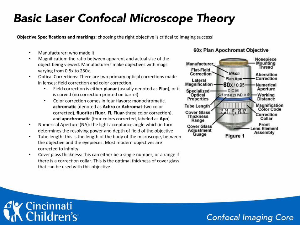
•  Manufacturer: who made it •  Magnifica%on: the ra%o between apparent and actual size of the

object being viewed. Manufacturers make objec%ves with mags varying from 0.5x to 250x.

•  Op%cal Correc%ons: There are two primary op%cal correc%ons made in lenses: field correc%on and color correc%on. •  Field correc%on is either planar (usually denoted as Plan), or it

is curved (no correc%on printed on barrel) •  Color correc%on comes in four flavors: monochroma%c,

achroma-c (denoted as Achro or Achromat-‐two color corrected), fluorite (Fluor, Fl, Fluar-‐three color correc%on), and apochroma-c (four colors corrected, labeled as Apo)

•  Numerical Aperture (NA): the light acceptance angle which in turn determines the resolving power and depth of field of the objec%ve

•  Tube length: this is the length of the body of the microscope, between the objec%ve and the eyepieces. Most modern objec%ves are corrected to infinity.

•  Cover glass thickness: this can either be a single number, or a range if there is a correc%on collar. This is the op%mal thickness of cover glass that can be used with this objec%ve.

Objec-ve Specifica-ons and markings: choosing the right objec%ve is cri%cal to imaging success!

Basic Laser Confocal Microscope Theory •  Working distance (WD): this is the distance between the front lens of the objec%ve and the cover glass when the specimen is in focus. Generally, higher mags = lower W, but long working distance (LWD) and extra/super/ultra-‐long working distance objec%ves (ELWD, SLWD, and ULWD, respec%vely) exist.

•  Special proper%es: this will denote if this objec%ve can be used for certain types of contrast, like Phase (denoted Ph) or differen%al interference (denoted DIC)

•  Immersion medium: this will be printed on the objec%ve barrel, or denoted by a colored ring.

•  Water is shown by a white ring, and W or Water is inscribed on the barrel

•  Oil is a black ring, and Oil or Oel is printed •  Glycerol is denoted by an orange ring, and Gly is on the barrel •  Special immersion media, or mul%-‐immersion objec%ves are

given a red ring •  Magnifica%on Color Codes (for objec%ves found on our systems):

•  4X: Red •  10X: Yellow •  20X: Green •  40X: Light Blue •  60X: Cobalt Blue •  100X: White

Basic Laser Confocal Microscope Theory

•  Aberra%ons and oddi%es: –  Chroma-c aberra-on: an aberra%on where different wavelengths of light are not focused in the same plane(axial), or

the different colors focus they focus at different posi%ons in the same focal plane (transverse) This can manifest itself in several ways. Either each color will appear in a different plane, or as spots in the same plane. Objects can also appear to have colored edges (known as purple-‐fringing). This is corrected by placing two types of glass together, usually crown glass and fluorite., and adjus%ng them so that the light focuses in the same spot in the same plane. At our level, chroma%c aberra%on can be mi%gated by using an achroma%c or apochroma%c lens (depending on the desired number of colors corrected).

–  Spherical aberra-on: an aberra%on where the image appears blurred due to unexpected diffrac%on of light. This is far more common that chroma%c aberra%on. A common cause is mixed media of differing refrac%ve indices. Make sure you match refrac%ve indices in your immersion media and moun%ng media as closely as possible. Do not allow for air gaps or bubbles! Another possible cause is using an objec%ve with a curved field. If this is unavoidable, try imaging in the lens’ aplana%c point. This is a certain area in the center of a lens that will not exhibit any spherical aberra%on. A common solu%on to spherical aberra%on is to use a Plan lens.

Getting Started 1.  Turn on the power strip on the right leg of the air table 2.  Turn the key on the laser launch 90° clockwise to the 3-‐9 posi%on 3.  Depress the buGon on the A1R controller

1 2

3

Getting Started

Log on to the computer, and begin NIS-‐Elements.

Image Acquisition Your screen should have been set up during your ini%al training. If for some reason it was not, contact Mike or MaG.

Right now, we will focus on single-‐dimension image acquisi%on (ie a single picture in a single focal plane). There are four major elements used in single-‐dimensional image collec%on:

•  Ti Pad •  A1plus Compact Gui •  OC (op%cal configura%ons) panel •  Scan Area

Ti pad

From here, you can change your objec%ves, light path, filter cubes, and adjust your Z-‐drive and lamp. You can also work with the Nikon Perfect Focus System. (PFS is not covered in this training) Ideally, the only %me you will use the Ti Pad is to change your objec%ve. Everything else is controlled by the OC Panel.

Selected objec%ve highlighted green

OC Panel

This is a macro-‐driven list of all of the established op%cal configura%ons in this microscope. You can add more, this is only a default list of common seungs. The top por%on controls the “eyes” por%on of the scope. It will set the light path to the appropriate port, and place the correct filter in the light path. The boGom por%on holds configura%ons for laser scanning. Each of the configura%ons shows what lasers are on, and some have special scanners and/or DIC/transmiGed light on. All of this is customizable.

A1plus Scan Area This dialogue allows you to change your scan size, type, and zoom. It also displays the current thickness of your op%cal sec%on (confocality!), your pixel size, dwell %me, and current resolu%on.

Band scan

Full frame scan

Polyline scan (rarely used)

Line scan Cancel zoom (full frame shortcut)

Update preview

Show zoom as large image

Scan Window: this is adjustable, so you can use either the window or the slider to adjust your zoom. Grab a corner, and resize it accordingly. Afer, you will be prompted to R-‐click to confirm, and the window will turn green again.

Scan size: can be changed here, but it is recommended to change it through the A1lus Compact GUI. Pixel size, z-‐step, resolu%on, and sec%on

thickness are all found here.

Nyquist XY: sets the zoom to the highest resolving limit per the Nyquist Theorem. Anything higher will not result in a gain in informa%on.

A1plus Compact GUI Scan, Capture, Find: Scan con%nually scans the image, it is a live view. Capture will take a snapshot of the current view. Find reduces the frame size and image quality to quickly acquire an area to scan. We do not train on the find func%on. Scanner selector: the galvanometric scanners are slower, but can provide more varia%on on scan area and longer pixel dwell %mes. The resonant is much faster, but with a short pixel dwell %me that may compromise resolu%on and image quality. Eye port: not used on this system. Remove Interlock: this is a physical shuGer that prevents lasing when the light path is sent to the eyes. It will turn red when it is on, and will need to be turned off when moving into confocal mode.

Unidirec-onal and bidirec-onal scanning (speed is gained, but resolu%on can be lost). If using bidirec%onal scanning, scan offset must be adjusted using the “…” buGon.

Pixel dwell -me/frames per second -me: determines how long the laser stays on one pixel. Longer %mes=more data and more laser. This can be good for areas of low signal, or very noisy areas. Be careful, however. Longer pixel dwell %mes can possibly lead to bleaching!

Scan size: this is the size, in pixels, of the area that you are scanning. The scan area is a square (in most cases), so this represents both the X and Y dimensions. More pixels=higher resolu%on (sort of-‐ it depends on the defini%on of resolu%on. The size of structure you can resolve is limited by the objec%ve’s NA. Image size gives you a larger raster, so the image can be displayed larger without loss of defini%on.

A1plus Compact GUI continued Normal/averaging/integra-on: averaging scans mul%ple lines and divides subsequent scans into each other, poten%ally reducing noise at the expense of longer scan %mes. Integra%on sums scans together, which can also poten%ally reduce noise, but we don’t train on it.

Channel Series: When this is ac%ve, the system will scan with one laser at a %me and collect image data on one PMT, minimizing crosstalk between channels. Scan %me is longer, but channel separa%on can be greatly improved. Next to it is the channel order buGon, where you can determine the order of the channel series. Pinhole Adjustment slider/AU buSon: the pinhole is important! It is what determines the size of the op%cal sec%on. A smaller pinhole means a thinner op%cal sec%on, and a larger pinhole gives more of a widefield-‐style of image (thicker slice). The AU buGon will op%mize the size of the pinhole for maximum axial resolu%on based on the longest wavelength of light that you are using.

Light path configura-on: this brings up the light path window. Please do not adjust any of these seungs without consul%ng Mike or MaG.

Laser Control Panel: with this, you can turn lasers and detectors on and off and adjust your laser power, gain, and offset. We will discuss this in more detail in image acquisi%on.

Image Acquisition Place your slide on the stage, coverslip down. On your OC Panel, click the “eyes” func%on corresponding to one of your fluorophores. Using the XY stage controller (to the right of the microscope) and the focus knobs on the microscope, find your sample. A good place to start is in a 1200-‐1400μm focal plane. Once you have found your sample and focused, select “Confocal” on the OC panel. Then, click on the correct op%cal configura%on for your sample. (ie which lasers, detectors, and scanners do you want on?)

Image Acquisition Click on “Remove Interlock,” and wait 3 seconds un%l it turns from red to subdued. Click “Scan.” A new window will pop up, and you will see your sample. If the image looks blank, increase HV and adjust focus to visualize the sample. At this point in %me, you need to begin op%mizing your image. Look at the top of the image window, and click on the satura%on indicator icon. This will highlight saturated pixels. It is a good idea to click the dropdown arrow next to it, and choose complementary colors. Also, if it is not already selected, choose to split your channels.

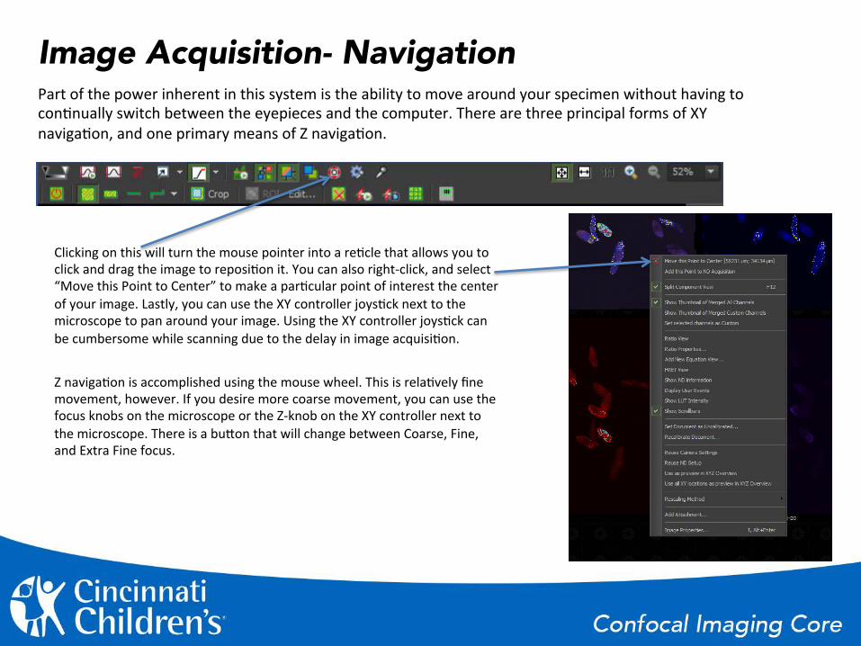
Image Acquisition- Navigation Part of the power inherent in this system is the ability to move around your specimen without having to con%nually switch between the eyepieces and the computer. There are three principal forms of XY naviga%on, and one primary means of Z naviga%on.

Clicking on this will turn the mouse pointer into a re%cle that allows you to click and drag the image to reposi%on it. You can also right-‐click, and select “Move this Point to Center” to make a par%cular point of interest the center of your image. Lastly, you can use the XY controller joys%ck next to the microscope to pan around your image. Using the XY controller joys%ck can be cumbersome while scanning due to the delay in image acquisi%on.

Z naviga%on is accomplished using the mouse wheel. This is rela%vely fine movement, however. If you desire more coarse movement, you can use the focus knobs on the microscope or the Z-‐knob on the XY controller next to the microscope. There is a buGon that will change between Coarse, Fine, and Extra Fine focus.

Image Acquisition- Saturation

This image, at first glance, looks okay. Looks can be deceiving, however. This image contains saturated pixels. With satura%on, image data points are falling outside the dynamic range of the detectors (PMTs). Above this range, the radiance of the pixel cannot be quan%fied.

Image Acquisition- Saturation

Turning on the satura-on indicator displays the currently saturated pixels on each channel. It is helpful to change the psuedocoloring of saturated pixels to “complementary color” using the dropdown to the right of the pixel satura%on indicator. The laser power and PMT gain can then be adjusted to minimize or eliminate saturated pixels.

Dropdown

Image Acquisition- Laser Power and Gain (HV) There is a golden rule to know: Use the lowest laser power necessary

to form an acceptable image. It is generally a good idea to start with low laser power and increase

the gain (HV) to brighten the image. Remember: the overall goal is to get an image with good signal-‐noise, not get a super bright image. At a certain point the gain becomes too high, and noise is unacceptable.

If you have maxed out your gain and you are s%ll not geung a good image (and you’re in a good focal plane), then drop the gain down, and slightly increase your laser power. Increasing laser power should be done carefully, especially at high magnifica%ons. More laser = more photons = increased possibility of bleaching or specimen damage. Once the laser power has been increased, try again increasing the gain un%l the image is sa%sfactory.

It is not recommended adjust the Offset slider, as this can clip low-‐intensity data. This low-‐intensity data can be fine-‐tuned in post-‐processing using LUTs.

Gain (HV)

Laser Power

Offset (don’t adjust)

Image Acquisition

When the PMT Gain and Laser Power are properly adjusted, you will get a good image, with no satura%on. Once you get a good image, click “Capture” on the A1plus Compact GUI to snap a picture of your scan area.

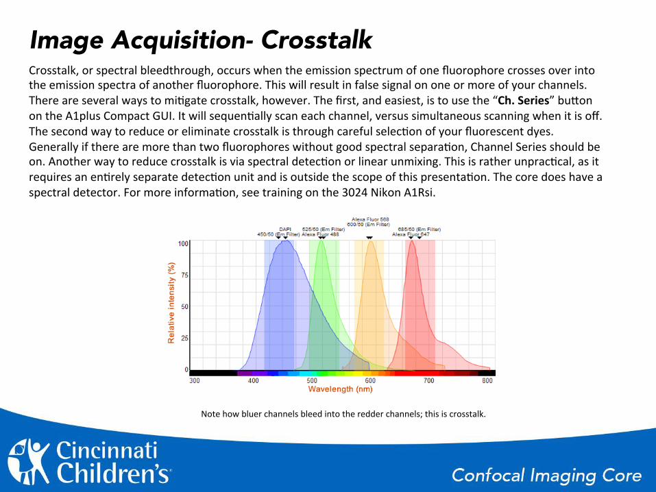
Image Acquisition- Crosstalk Crosstalk, or spectral bleedthrough, occurs when the emission spectrum of one fluorophore crosses over into the emission spectra of another fluorophore. This will result in false signal on one or more of your channels. There are several ways to mi%gate crosstalk, however. The first, and easiest, is to use the “Ch. Series” buGon on the A1plus Compact GUI. It will sequen%ally scan each channel, versus simultaneous scanning when it is off. The second way to reduce or eliminate crosstalk is through careful selec%on of your fluorescent dyes. Generally if there are more than two fluorophores without good spectral separa%on, Channel Series should be on. Another way to reduce crosstalk is via spectral detec%on or linear unmixing. This is rather unprac%cal, as it requires an en%rely separate detec%on unit and is outside the scope of this presenta%on. The core does have a spectral detector. For more informa%on, see training on the 3024 Nikon A1Rsi.

Note how bluer channels bleed into the redder channels; this is crosstalk.

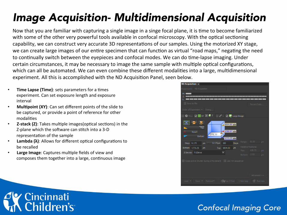
Image Acquisition- Multidimensional Acquisition Now that you are familiar with capturing a single image in a singe focal plane, it is %me to become familiarized with some of the other very powerful tools available in confocal microscopy. With the op%cal sec%oning capability, we can construct very accurate 3D representa%ons of our samples. Using the motorized XY stage, we can create large images of our en%re specimen that can func%on as virtual “road maps,” nega%ng the need to con%nually switch between the eyepieces and confocal modes. We can do %me-‐lapse imaging. Under certain circumstances, it may be necessary to image the same sample with mul%ple op%cal configura%ons, which can all be automated. We can even combine these different modali%es into a large, mul%dimensional experiment. All this is accomplished with the ND Acquisi%on Panel, seen below.

•  Time Lapse (Time): sets parameters for a %mes experiment. Can set exposure length and exposure interval

•  Mul-point (XY): Can set different points of the slide to be captured, or provide a point of reference for other modali%es

•  Z-‐stack (Z): Takes mul%ple images(op%cal sec%ons) in the Z-‐plane which the sofware can s%tch into a 3-‐D representa%on of the sample

•  Lambda (λ): Allows for different op%cal configura%ons to be recalled

•  Large Image: Captures mul%ple fields of view and composes them together into a large, con%nuous image

ND Acquisition- Time Lapse

Time Lapse allows for measurement across %me. Mul%ple phases can be entered into the experiment. For each phase an interval (frequency of measurement) and a dura%on (length of measurement) needs to be chosen. Afer the correct parameters have been entered, click “Run now” to begin the experiment.

ND Acquisition- Multipoint XY is the mul%point modality of the ND Acquisi%on Panel. It will store mul%ple XY (and Z, if Include Z is checked) points that can be used in other modali%es. To add a point, simply click on the checkbox in the point name field. The fields will be populated with the center of the image that you are currently viewing. X and Y can be manually entered, as well. Clicking the liGle arrow next to the point name will update the point informa%on to the spa%al data of the center of your current field of view. Clicking “Run now” without any other modali%es will take single images of each point in the XY tab.

ND Acquisition- Large Image

Large Image will s%tch together mul%ple fields to create a large composite image. This is good for u%lizing a higher-‐NA objec%ve to get beGer resolu%on for a specimen that cannot fit into a single field of view. It is also excellent for crea%ng a spa%al road map of the en%re area of interest, as XY data will be encoded into the final image. Large Image must be used in conjunc-on with another modality, such as XY or Time Lapse. (circle phases on image) To use, choose either the number of fields in X and Y, or choose X and Y dimensions in mm. It is advisable to use the default 15% overlap for s%tching. The sofware will account for this, and make any image adjustments as necessary. There is no need to account for the extra 15% when entering fields or mm. When the size is set and an addi%onal modality is chosen, click “Run now” to begin the experiment.

ND Acquisition- Z-stack

There are three choices for Z-‐stacking. The first is define top and boSom with absolute posi%on. In this, you choose the top and boGom of the stack. The reset buGon will reset all of your points. Simply navigate to the top of your stack, and click the “Top” buGon, and do the same for the “BoGom.” If you get them backwards, don’t worry. The sofware is smart that way. It will fix it for you. When you have chosen your points and the proper step size, click “Run now” to begin. Z-‐stack does not require and addi%onal modality.

Step size field

Op%mal step size buGon

Z device selector Piezo homing buGon (when Piezo device is selected)

When you have built your Z-‐stack, you can double-‐click on each of the three points to check your stack. It is good to check your seungs at the top, middle, and boGom to ensure nothing is amiss. For example, if you are using the Piezo Z-‐drive and your sec%on is larger than 200 microns, it will change one of the sets points to limit the range.

I’m confused! What’s all this talk about step size, and why do I have a choice of Z devices? Good ques%on! Step size is important, because it is derived from the thickness of your current op%cal sec%on. Nikon recommends a ~66% overlap between op%cal sec%ons when construc%ng a Z-‐stack so it will s%tch together nicely. It is acceptable to use less than that, but you never want your step size to be larger than your op%cal sec%on. You lose data that way. There is a buGon next to the step size field that will automa%cally select the op%mal step size. There are several Z devices to choose from, too. They have different speeds and different ranges of mo%on. The Piezo Z is fast, but it is limited to 200μm in thickness. The normal Z drive is slower, but there is virtually no limit to the thickness of your Z sec%on aside from the working distance of the lens (and the ability of light to penetrate your sample, but that’s another lesson!).

ND Acquisition- Z-stack

ND Acquisition- Z-stack symmetrical

The second choice in Z-‐stacking is symmetrical stacking. This will take a range above and below an absolute point. You need to specify the range in the range field, and the step size, just like before. Pressing the “Rela%ve” buGon will keep your range, and allow you to change your absolute point as you mouse up and down. Pressing “Home” will make your current Z posi%on the absolute point. When all parameters are set, press “Run now” to begin the experiment.

ND Acquisition- Z-stack asymmetrical

The third choice in Z-‐stacking is asymmetrical stacking. This will take a range above and below an absolute point, but in this instance you must specify how much above and below you would like the sofware to image. You need enter the distance above and below in the respec%ve fields and the step size, just like before. Pressing the “Rela%ve” buGon will keep your range, and allow you to change your absolute point as you mouse up and down. Pressing “Home” will make your current Z posi%on the absolute point. When all parameters are set, press “Run now” to begin the experiment.

ND Acquisition- Lambda (λ)

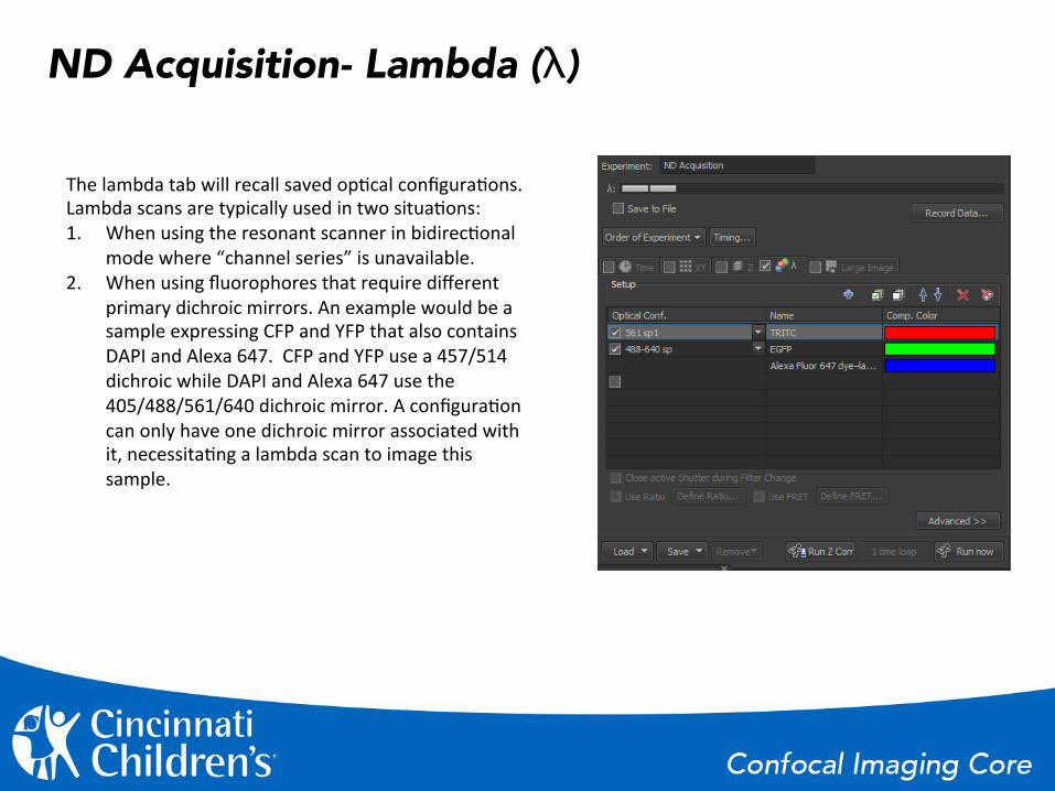
The lambda tab will recall saved op%cal configura%ons. Lambda scans are typically used in two situa%ons: 1.  When using the resonant scanner in bidirec%onal

mode where “channel series” is unavailable. 2.  When using fluorophores that require different

primary dichroic mirrors. An example would be a sample expressing CFP and YFP that also contains DAPI and Alexa 647. CFP and YFP use a 457/514 dichroic while DAPI and Alexa 647 use the 405/488/561/640 dichroic mirror. A configura%on can only have one dichroic mirror associated with it, necessita%ng a lambda scan to image this sample.

Tying it all together The first ques%on you should ask yourself is “what are the goals of my imaging?” The last thing you want to do is to spend most of your %me fumbling around trying to find something, or poorly image something mul%ple %mes only to see your %me run out. If you create a good plan in advance, then you can op%mize your %me on the system, and get the most bang for your buck. Do you need to see the en%re slide, or do you have a large mount? Don’t waste %me trying to image the whole thing right off the bat with the Galvo. Switch to the resonant, and take a large image much faster. Find your area of interest, then switch to the Galvo scanner. A large image at a low mag contains the same spa%al informa%on as one at high mag, but your fields are much larger. If you need to take a large image, maybe do it at a low mag, then choose a good ROI for higher mag. Higher magnifica-on isn’t always beSer. Remember, your resolu%on is driven by the numerical aperture of your objec%ve lens. A 20X with a NA of 0.8 will resolve down to .37 microns at 488nm. A 40x with a 1.0 NA will resolve down to .29 microns at 488. Occasionally that eight nanometers may maGer, but more ofen than not it will not hinder your imaging to be at a lower magnifica%on. Axial (Z) resolu%on is also determined by your NA. It is generally (but not always) half of the lateral resolu%on. This is due to the point spread func%on of light. Without geung to physics-‐heavy, it goes to say that a higher NA=thinner op%cal sec%on=less lower-‐intensity, out of focus light in the point spread func%on. Tailor your objec-ve to your imaging needs! Experience will be your best friend, but if you need assistance, we are always here to help.

Image Size, Scan Zoom, and Photobleaching The image size (or scan format) is the number of X-‐Y pixels that the scanner is collec%ng in a single pass of the image. The smaller the scan format (ie 512), the larger the pixel, thus the lower the resolu%on of the image. A larger scan format (ie 1024) will result in a smaller pixel, and a higher resolu%on image. Higher scan formats take longer to acquire, however. Confocal microscopes with galvanometric scanning mirrors are able to change the oscilla%on angle of the mirrors and scan a smaller area while maintaining the same number of pixels. This is called scan zoom. You cannot arbitrarily keep zooming in, though. At a certain point, oversampling will not add any more defini%on to the image. This is known as the Nyquist Limit (as discussed in Confocal Microscope Theory earlier on). Past the Nyquist Limit there is no addi%onal data added to the image, and resolu%on cannot be increased any further. Zooming and changing your image size can affect your pixel dwell %me and the number of incident photons over the sampled area. Too much light can lead to photobleaching or possible photodamage of the specimen. This is to be avoided at all costs, as it is unrecoverable.

Image Size, Scan Zoom, and Photobleaching

Before and afer of severe photobleaching from the laser. Laser photobleaching is always square. If you see round areas of dimmed fluorescence, it is bleaching caused by the epifluorescent light source. Decrease your light power. It is recommended that you scan away from your area occasionally to check for signs of photobleaching, especially if you are working for long periods of %me at high mag, high zooms, high power, or high pixel dwell %mes.

Changing Objectives and Immersion Media There will be a need to change from a dry objec%ve to an immersion objec%ve, and that’s perfectly acceptable. There is a simple way to do this. 1.  Capture your image at a lower magnifica%on. 2.  Change to the immersion objec%ve using the Ti Pad. Do not use the buGons on the microscope! 3.  Press the “Escape” buGon on the right side of the microscope. 4.  Use the XY Joys%ck to expose the objec%ve. 5.  Apply the immersion media. 6.  Right click on your image, and select a point to move to center. 7.  Press “Refocus” on the right side of the microscope. Some%mes, you will have to use your eyes to adjust the focus, but more ofen than not you will be very close to the same focal plane as before. The only small difference will be due to the changing refrac%ve index of the immersion media. Once on immersion objec-ve, DO NOT RETURN TO DRY OBJECTIVE WITHOUT PROPERLY CLEANING YOUR SLIDE

Shutting Down and Leaving the System First, remove your slide. Clean any immersion media off the objec%ve using lens paper. Using the Ti pad, change to a lower magnifica%on (10X or lower). Manually lower the objec%ve using the focus knobs to 500μm or lower. Check the booking schedule at research.cchmc.org/mrbs. If someone is scheduled soon afer you (within an hour or two) simply log off the computer and go about your day. If no one is afer you, or you are the last user of the day, shut down is the opposite of start up. 1.  Log off the computer. 2.  Depress the buGon on the A1 controller box. 3.  Turn the key on the laser launch back to the 12-‐6 posi%on. 4.  Turn off the power strip on the right leg of the microscope table.

A final note…

SPIN YOUR ANTIBODIES!

•  really, really give them a good whirl •  vortex your primary, and spin it at max speed (12K rpm+

for at least 10 minutes) •  make your dilu%on using the supernatant, and spin it for

at least 10 minutes at max speed •  apply that supernatant •  repeat for the secondary an%body

Nikon A1R GaAsP Laser Scanning Confocal Microscope

Documents

Transcript of Nikon A1R GaAsP Laser Scanning Confocal Microscope