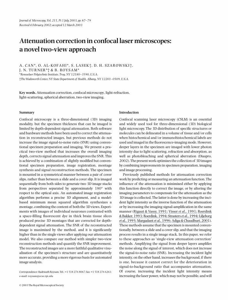
© 2003 The Royal Microscopical Society

Journal of Microscopy, Vol. 211, Pt 1 July 2003, pp. 67–79

Received 4 February 2002; accepted 12 March 2003

Blackwell Publishing Ltd.

Attenuation correction in confocal laser microscopes: a novel two-view approach

A . C A N *, O. A L - KO F A H I *, S . L A S E K †, D. H . S Z A R OW S K I †, J. N. TU R N E R *† & B . RO Y S A M *

*

Rensselaer Polytechnic Institute, Troy, NY 12180–3590, U.S.A.

†

The Wadsworth Center, NY State Department of Health, Albany, NY 12201–0509, U.S.A.

Key words.

Attenuation correction, confocal microscopy, light-refraction, light-scattering, spherical aberration, two-view imaging.

Summary

Confocal microscopy is a three-dimensional (3D) imagingmodality, but the specimen thickness that can be imaged islimited by depth-dependent signal attenuation. Both softwareand hardware methods have been used to correct the attenua-tion in reconstructed images, but previous methods do notincrease the image signal-to-noise ratio (SNR) using conven-tional specimen preparation and imaging. We present a pra-ctical two-view method that increases the overall imagingdepth, corrects signal attenuation and improves the SNR. Thisis achieved by a combination of slightly modified but conven-tional specimen preparation, image registration, montagesynthesis and signal reconstruction methods. The specimenis mounted in a symmetrical manner between a pair of coverslips, rather than between a slide and a cover slip. It is imagedsequentially from both sides to generate two 3D image stacksfrom perspectives separated by approximately 180

°

withrespect to the optical axis. An automated image registrationalgorithm performs a precise 3D alignment, and a model-based minimum mean squared algorithm synthesizes amontage, combining the content of both the 3D views. Experi-ments with images of individual neurones contrasted witha space-filling fluorescent dye in thick brain tissue slicesproduced precise 3D montages that are corrected for depth-dependent signal attenuation. The SNR of the reconstructedimage is maximized by the method, and it is significantlyhigher than in the single views after applying our attenuationmodel. We also compare our method with simpler two-viewreconstruction methods and quantify the SNR improvement.The reconstructed images are a more faithful qualitative visu-alization of the specimen’s structure and are quantitativelymore accurate, providing a more rigorous basis for automatedimage analysis.

Introduction

Confocal scanning laser microscopy (CSLM) is an essentialand widely used tool for three-dimensional (3D) biologicallight microscopy. The 3D distribution of specific structures ormolecules can be delineated in a volume of tissue and/or cellswhen histochemical and/or immunohistochemical labels areused and imaged in the fluorescence-imaging mode. However,deeper layers in the specimen are imaged with lower photonintensity due to light scattering, refraction and absorption, aswell as photobleaching and spherical aberration (Diaspro,2002). The present work optimizes the collection of 3D imagesby combining improvements in specimen preparation, imagingand image processing.

Previously published methods for attenuation correctionwork by predicting or measuring an attenuation function. Theinfluence of the attenuation is minimized either by applyingthis function directly to correct the image, or by altering theimaging parameters to compensate for the attenuation as the3D image is collected. The latter is done by increasing the inci-dent light intensity as the inverse function of the attenuationor by increasing the imaging signal-amplification in the samemanner (Rigaut & Vassy, 1991; Visser

et al

., 1991; Roerdink& Bakker, 1993; Roerdink, 1994; Strasters

et al

., 1994; Liljeborg

et al

., 1995; Margadant

et al

., 1996; Adiga & Chaudhuri, 2001).These methods assume that the specimen is mounted conven-tionally, between a slide and a cover slip, and that the imagingprocess results in a single image stack. In this paper, we referto these approaches as ‘single-view attenuation correction’methods. Amplifying the signal from deeper layers amplifiesthe noise along the signal of interest, which does not increasethe signal-to-noise ratio (SNR). Increasing the incident lightintensity, on the other hand, increases the background, if thereis one, because it cannot correct for the deterioration insignal-to-background ratio that accompanies attenuation.Of course, increasing the incident light intensity meansincreasing the laser power, which may not be possible, and will

Correspondence: Badrinath Roysam. Tel.: +1 518 276 8067; fax: +1 518 276 6261;

e-mail: roysam@ecse.rpi.edu

68

A . CA N

E T A L .

© 2003 The Royal Microscopical Society,

Journal of Microscopy

,

211

, 67–79

exacerbate photobleaching. Current methods often assumethat the fluorochrome distribution in the specimen is uniform.This assumption is rarely valid for biological specimens thatare composed of very complex structures often with complexmorphologies and large variations of label.

Previous attempts have been made to reconstruct micro-scope images from multiple views. These attempts, however,are aimed at increasing the axial resolution rather than theimaging depth (Mastronarde, 1997; Frank, 2001). This hasbeen thoroughly addressed in the field of electron micros-cope tomography. In widefield microscopy (Shaw

et al

., 1989;Shaw, 1990), and in confocal microscopy (Cogswell

et al

.,1996; Heintzmann

et al

., 2000), multiple views (tilted views)were also used to increase the axial resolution. Special speci-men preparation inside a capillary or on a glass fibre and aspecial tilt stage were needed. For confocal light microscopy,this approach limits the spatial extent of the specimen that canbe imaged. The present work calls for much simpler prepara-tion and imaging instrumentation, and allows imaging ofspecimens essentially unlimited in the

x, y

directions (Can

et al

., 2000).

Discussion of single-view attenuation correction methods

The current methods attempt to correct a single stack ofoptical slices. There are two basic approaches in use. One type(exemplified by Rigaut & Vassy, 1991; Liljeborg

et al

., 1995;Nagelhus

et al

., 1996; Adiga & Chaudhuri, 2001) relies ona statistical model, whereas the other (exemplified by Visser

et al

., 1991; Roerdink & Bakker, 1993; Roerdink, 1994;Strasters

et al

., 1994; Margadant

et al

., 1996) uses geometricmodels. Both methods first compute a one-dimensional (alongthe

z

-axis) spatial correction factor based on the statisticalor geometric model, and then adjusts the intensity at a given

z

-dimension (slice) with a multiplicative correction factor.The statistical methods of attenuation correction estimate

the distribution of the intensity as a function of depth by form-ing histograms and fitting curves. While they are computa-tionally attractive, and can also take photobleaching intoaccount, they suffer from two main limitations. First, theirapplicability is limited to specimens with nearly homogeneousfluorochrome distribution, especially as a function of depth.This is a condition rarely found in biological specimens. Forexample, in neuron images such as those shown in Al-Kofahi

et al

. (2003), the fluorochrome density is mostly a function ofthe spatial locations of the dendrites and the soma. Since thesoma has a complex 3D shape, the intensity variation betweenconsecutive slices is a function of its geometry as well as of theattenuation. A second drawback of statistical methods is thelack of improvement in SNR. This is because attenuationcorrection based on multiplying by a factor amplifies the noiseas well as the signal.

The geometrical optics-based methods closely represent theunderlying optical phenomena, but also suffer from the SNR

problem noted above for statistical methods. Additionally,they are more computationally intensive, and estimatingsome of the related parameters is difficult. These methods arebased on the assumption that the image intensity is a functionof fluorochrome density, and iteratively corrects the layers.Visser

et al

. (1991) described the underlying optical geometry,and a reconstruction algorithm based on a layer strippingmethod. The light bundle is assumed to travel as a sphericalwave that converges to the focal point and forms a cone structure(Fig. 1). The attenuation of excitation and florescence light iscomputed by integrating all light paths within this conicalvolume. This method does not correct for photobleaching orspherical aberration; the latter becomes more prominentwhen the refractive indices of the mounting and immersionmedia are mismatched (Hell

et al

., 1993; Jacobsen

et al

., 1994).It is also not very practical due to its high computational com-plexity (scales with the fourth power of image depth, i.e.

O

( ),

N

z

is the depth of the image), especially for the high-resolutionimages where the depth resolution is high. Following themodel description of Visser

et al

. (1991), Roerdink & Bakker(1993) reformulated the problem by 3D convolution integralsto reduce the computational time to

O

(

N

z

log

N

z

). Obtainingslightly lower-quality results under their weak attenuationassumption, this method suffers from a high memory require-ment, which is a major problem for high-resolution images.Roerdink (1994) improved the accuracy of this method byreformulating the problem as a statistical estimation problem.By using a similar cone structure, Margadant

et al

. (1996)reduced the computational memory requirements. Using theimage plane sampling for ray discretization, Strasters

et al

.(1994) proposed two computationally efficient methods,recursive attenuation correction using directional extinctiontracking (RAC-DET) and recursive attenuation correctionusing light front tracking (RAC-LT). In these methods, atten-uation information at the previous slice is used to calculatethe attenuation coefficients at the current slice. In our work,we modified the RAC-DET algorithm for single-view attenua-tion correction to correct for spherical aberration, in additionto scattering and absorption.

In summary, the limitations of the single-view methodsbased on statistical or geometric models are:1 They do not provide any gain in terms of SNR because the

noise and the signal are simultaneously amplified.2 The parameters of the models are estimated based on the

assumption that the fluorochrome density is constant along thedepth, which is not true for most types of biological specimen.

Overview of the proposed two-view method

The concept underlying the proposed two-view method issimple. In this method, the corrected image is an attenuation-corrected montage of two images taken from different viewsof the specimen. In other words, the specimen is flipped overwithout special instrumentation (i.e. an inexact flip), and

N z4

T WO - V I E W C O N F O CA L I M AG E AT T E N UAT I O N C O R R E C T I O N

69

© 2003 The Royal Microscopical Society,

Journal of Microscopy

,

211

, 67–79

imaged again from the opposite direction to collect a second3D image. The two views are separated by approximately180

°

. Structures that appear to be darker in the deeper layersof one view are at the shallow layers in the other view, andtherefore appear bright.

The above simple concept requires attention to several pra-ctical issues. For example, the specimen must be prepared in amanner suitable for symmetrical imaging. Second, computeralgorithms are required for precise registering of the two views(Al-Kofahi

et al

., 2003). The intensity values and correctioncoefficients of the two registered views must be combined insuch a way that the reconstructed montage image has ahigher SNR compared to either corrected single view. Thismontage can be used to increase the depth and extent ofimaging in confocal microscopes. Extended structures suchas neurones represent a good initial test specimen to evaluatethe overall methodology.

Specimen preparation

To enable two-sided symmetric imaging (Fig. 1), the specimenis mounted between two cover slips using a spacer. A 3D imageset is collected in the conventional way then the sample is flippedupside down and imaged again. The perspectives of the two3D images are approximately 180

°

apart. Figure 2 shows thethree orthogonal projections of typical two-view 3D images ofa neuron from the hippocampus of Wistar rat brain. The brainis perfusion fixed in buffered 4% paraformaldehyde, removedfrom the carium, blocked and thick (300-

µ

m) sections cut ona vibratome. All procedures were in accordance with theguidelines of the NIH and the Animal Care Committee of theWadsworth Center.

Individual neurones were filled in the thick slices with 4%Alexa 594 (Molecular Probes, Eugene, OR, U.S.A.). Slices weremounted in an injection chamber and placed on the stage of

Fig. 1. Illustration of the imaging model. Top: theconversion of the monochromatic plane wave into aconverging spherical wave, bounded by the semi-aperture angle ω, with radius R. Bottom: illustrationof the two-view imaging model. The specimen isimaged from two angles separated by approximately180°, and then reconstructed using computationalmethods to complete the thick image. To enable two-sided symmetric imaging, the specimen is mountedbetween two cover slips using a spacer. The coordinatesystem of the first image is used as the coordinatesystem for the reconstructed image.

70

A . CA N

E T A L .

© 2003 The Royal Microscopical Society,

Journal of Microscopy

,

211

, 67–79

a microscope equipped for epi-fluorescence microscopy. Theslices were penetrated, under visual control, by a sharp,borosilicate glass micropipette loaded with the dye. Dye wascontinuously ejected ionophoretically with 250-ms, 2-Hz

negative current pulses. The pipette was advanced throughthe tissue until the cell body of a neuron appeared to fill withand retain the dye. At this point the electrode was halted anddye was injected until all the dendrites were completely filled

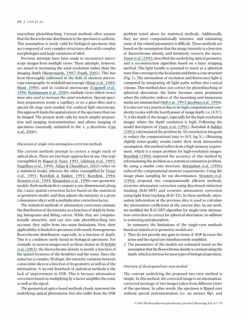
Fig. 2. Sample views of an Alexa 594 filled neuron; the left-column is view-1 and the right column is view-2. The top row shows x–y maximum-valuefiltered projections, and the second and third rows show x–z and y–z projections, respectively. Notice that in the deeper layers, the dendrites are dimmer due toattenuation. View-2 is the image of the same specimen after flipping as illustrated in Fig. 1. The neuronal processes in the deeper layers in view-1 are now inthe upper layers in view-2, and appear brighter. The sampling rates are 0.375 µm pixel−1 for the X and Y dimensions and 0.5 µm pixel−1 for the Z dimension.

T WO - V I E W C O N F O CA L I M AG E AT T E N UAT I O N C O R R E C T I O N

71

© 2003 The Royal Microscopical Society,

Journal of Microscopy

,

211

, 67–79

and dendritic tips fluoresced brightly. After several cells wereinjected within each slice, the slice was post-fixed for 1.5 h inthe same fixative. The tissue slices were mounted in 95% buff-ered glycerol with 1% n-propyl gallate in a well formed by athin spacer between two cover slips. This allows the slice to beimaged from both directions.

The images were collected using a NORAN Oz confocalattachment on an Olympus IX-70 inverted infinity-correctedmicroscope, using a 40

×

NA 1.15 water immersion objectivelens and with a field size of 192

×

180

µ

m and 0.375

µ

m pixel

−

1

.The

z

-direction step size is 0.5

µ

m pixel

−

1

for the images shownin Fig. 2.

Mathematical models describing the imaging process

This section summarizes the key mathematical models andassumptions used by the two-view correction method. Ourwork draws heavily from the single-view correction work ofStrasters

et al

. (1994). First we describe the imaging process ofa CSLM in the fluorescence mode for a single-view operation,and then we describe the attenuation correction in a two-viewsystem. Our model corrects for four sources of signal attenua-tion: absorption, scattering, refraction and spherical aberra-tion (Diaspro, 2002). Note, however, that the goal of this workis not to describe an exact model for the optical attenuationphenomenon in the confocal microscope but, rather, wedescribe the two-view imaging model and its application toattenuation correction. Simplified mathematical derivationswill be presented in this section; for a more rigorous discussion,the reader is referred to Appendix A at the end of this paper.

Attenuation due to absorption is negligible in homogenousspecimens with no high dye concentration (de Grauw

et al

.,1999; Diaspro, 2002). However, in regions where the dyeconcentration is significantly high (e.g. soma or cell body inneuron images), absorption has to be taken into account.Scattering occurs when the excitation or the fluorescentlyemitted light is incident on objects with different refractiveindices that are smaller than the wavelength; if the object islarger than the wavelength, refraction occurs.

In fluorescence microscopy, the excitation and emission wavel-engths are different, implying that the attenuation coefficientsare different for the exciting and emitted light. The equationthat describes the signal attenuation on the way to and from thefocus point is given by Diaspro (2002) and Flock

et al

. (1992)

(1)

where

I

(

z

,

λ

) is the collected light, which is a function of thefocal position (see Fig. 1) and the wavelength,

λ

, used.

α

exc

and

α

em

are the attenuation coefficients for the exciting andemitted light, respectively; these describe attenuation due toabsorption, scattering and refraction. For more details on thegeometry of the specimen, and calculation of the distance

z

in(1) above, see Appendix A.

The effect of spherical aberration is enhanced due to refrac-tive index mismatch between the immersion medium andthe mounting medium, and broadens the PSF as a result. Theextent of the broadening increases with depth, which resultsin loss of signal passing through the pinhole (Carlsson, 1991).Spherical aberration is modelled in this article as exponentialsignal attenuation as a function of depth. This is not an accu-rate model, but it is used here for convenience.

If we incorporate the spherical aberration effect with thosedue to absorption, scattering and refraction, then the originalintensity that we wish to recover,

Î

(

x

), is related to theobserved intensity,

I

(

x

), by the following relationship:

I

(

x

) =

γ

sph

(

z

)

γ

exc

(

x

)

γ

em

(

x

)

Î

(

x

), (2)

where

γ

sph

(

z

) is the attenuation factor due to spherical aberra-tion.

γ

exc

(

x

) and

γ

em

(

x

) are the excitation and emitted lightattenuation factors, respectively. These factors can be arrangedto be equal to unity if there is no attenuation, and can bewritten (see Appendix A) as:

(3)

(4)

(5)

where

α

sph

is the spherical aberration extinction coefficient.For our neuron specimen images, attenuation due to spher-

ical aberration appears to be the most significant for most ofthe specimen volume that is not occluded by the soma (regionswith low fluorochrome density), while absorption is significantin the region beneath the soma (high fluorochrome density).

Application of the imaging model to single-view correction

Excluding spherical aberration, algorithms to solve Eq. (2)have been described by Visser

et al

. (1991), Roerdink & Bakker(1993), Roerdink (1994) and Strasters

et al

. (1994). Theoriginal image is reconstructed by multiplying the observedintensity by a spatial correction constant

C

(

x

),

Î

(

x

) =

C

(

x

)

I

(

x

); (6)

where

(7)

is the inverse of the overall attenuation.

I z I z I e eexc emz zexc em( , ) exp [ ( ) ] ,λ α α α α= − + = − −

0 0

γ αsph

zz e sph( ) = −

γπ ω

θ θ φ θ

ω π αθ

exc

z

e

z

exc

( ) sin

cos sin ;

( )cos

x

x

=− ′

′12

0 0

2

0�� � d

d d

γπ ω

θ φ θ

ω π αθ

em

z

e

z

em

( ) ( cos )

sin .

( )cos

x

x

=−

− ′′1

2 10 0

2

0�� � d

d d

Czsph exc em

( ) ( ) ( ) ( )

xx x

=1

γ γ γ

72 A . CA N E T A L .

© 2003 The Royal Microscopical Society, Journal of Microscopy, 211, 67–79

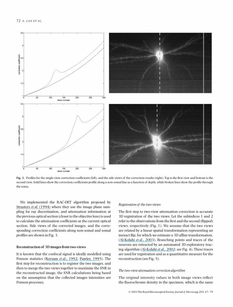
We implemented the RAC-DET algorithm proposed byStrasters et al. (1994) where they use the image plane sam-pling for ray discretization, and attenuation information atthe previous optical section (closer to the objective lens) is usedto calculate the attenuation coefficients at the current opticalsection. Side views of the corrected images, and the corre-sponding correction coefficients along non-somal and somalprofiles are shown in Fig. 3.

Reconstruction of 3D images from two-views

It is known that the confocal signal is ideally modelled usingPoisson statistics (Roysam et al., 1992; Pawley, 1995). Thefirst step for reconstruction is to register the two images, andthen to merge the two views together to maximize the SNR inthe reconstructed image, the SNR calculations being basedon the assumption that the collected images intensities arePoisson processes.

Registration of the two-views

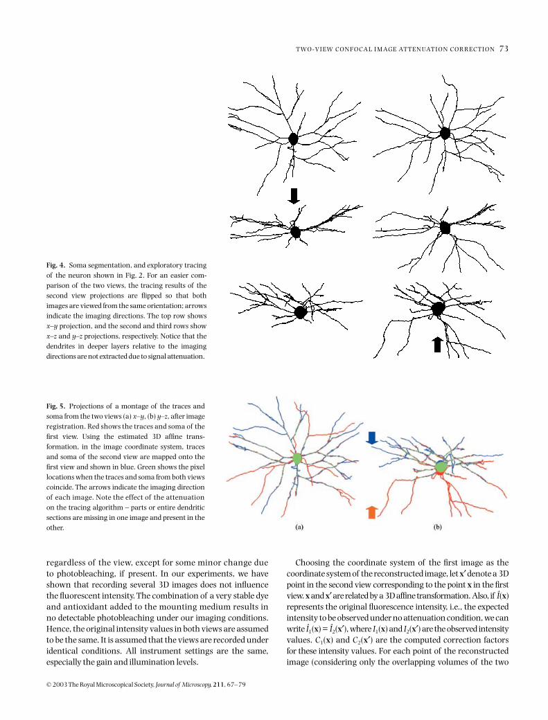
The first step to two-view attenuation correction is accurate3D registration of the two views. Let the subindices 1 and 2refer to the observations from the first and the second (flipped)views, respectively (Fig. 1). We assume that the two viewsare related by a linear spatial transformation representing aninexact flip, for which we estimate a 3D affine transformation.(Al-Kofahi et al., 2003). Branching points and traces of theneurons are extracted by an automated 3D exploratory trac-ing algorithm (Al-Kofahi et al., 2002; see Fig. 4). These tracesare used for registration and as a quantitative measure for thereconstruction (see Fig. 5).

The two-view attenuation correction algorithm

The original intensity values in both image views reflectthe fluorochrome density in the specimen, which is the same

Fig. 3. Profiles for the single-view correction coefficients (left), and the side views of the correction results (right). Top is the first view and bottom is thesecond view. Solid lines show the correction coefficients profile along a non-somal line as a function of depth, while broken lines show the profile throughthe soma.

T WO - V I E W C O N F O CA L I M AG E AT T E N UAT I O N C O R R E C T I O N 73

© 2003 The Royal Microscopical Society, Journal of Microscopy, 211, 67–79

regardless of the view, except for some minor change dueto photobleaching, if present. In our experiments, we haveshown that recording several 3D images does not influencethe fluorescent intensity. The combination of a very stable dyeand antioxidant added to the mounting medium results inno detectable photobleaching under our imaging conditions.Hence, the original intensity values in both views are assumedto be the same. It is assumed that the views are recorded underidentical conditions. All instrument settings are the same,especially the gain and illumination levels.

Choosing the coordinate system of the first image as thecoordinate system of the reconstructed image, let x′ denote a 3Dpoint in the second view corresponding to the point x in the firstview. x and x′ are related by a 3D affine transformation. Also, if Î(x)represents the original fluorescence intensity, i.e., the expectedintensity to be observed under no attenuation condition, we canwrite Î1(x) = Î2(x′), where I1(x) and I2(x′) are the observed intensityvalues. C1(x) and C2(x′) are the computed correction factorsfor these intensity values. For each point of the reconstructedimage (considering only the overlapping volumes of the two

Fig. 4. Soma segmentation, and exploratory tracingof the neuron shown in Fig. 2. For an easier com-parison of the two views, the tracing results of thesecond view projections are flipped so that bothimages are viewed from the same orientation; arrowsindicate the imaging directions. The top row showsx–y projection, and the second and third rows showx–z and y–z projections, respectively. Notice that thedendrites in deeper layers relative to the imagingdirections are not extracted due to signal attenuation.

Fig. 5. Projections of a montage of the traces andsoma from the two views (a) x–y, (b) y–z, after imageregistration. Red shows the traces and soma of thefirst view. Using the estimated 3D affine trans-formation, in the image coordinate system, tracesand soma of the second view are mapped onto thefirst view and shown in blue. Green shows the pixellocations when the traces and soma from both viewscoincide. The arrows indicate the imaging directionof each image. Note the effect of the attenuationon the tracing algorithm – parts or entire dendriticsections are missing in one image and present in theother.

74 A . CA N E T A L .

© 2003 The Royal Microscopical Society, Journal of Microscopy, 211, 67–79

3D images after registration) we have two readings from thetwo different views.

Modelling the confocal signal for the hypothetical unatten-uated image by a Poisson process and using the MaximumLikelihood (ML) estimator to reconstruct the image from thetwo views, we get:

(8)

is the estimated reconstructed intensity. Notice that theML estimator is unbiased, i.e. . Let be theresulting SNR in the two-view reconstructed image, andSNR be that which would have been observed under the no-attenuation condition, Î(x). Then

(9)

The in Eq. (9) is identical to that achieved using a simpleaverage of the two views as shown in the equation below:

(10)

However, reconstruction using the average of the two viewsis biased, i.e.

(11)

Figure 6 shows the result of registering the two views shownin Fig. 2, and reconstructing the image using Eq. (8). Usingthe ML estimator for reconstruction is also intuitively satisfy-ing. Notice that for locations where the attenuation is high inthe second view, places such as the deeper layers or beneaththe soma, C2(x′) >> C1(x) ≥ 1, the reconstructed image isformed predominantly from the first view, ,which has a higher SNR at this location. Similarly, the deeperlayers in the first view contribute less to the reconstructedimage at the corresponding 3D location than does the secondview. For the locations where the attenuation values on bothviews are comparable, C2(x′) ≈ C1(x), Eq. (8) gives the averageof both corrected views

(12)

Another possible approach for reconstruction from the twoviews is to weight the two views inversely proportional withrespect to the depth from the viewing direction when averag-ing. This method produces a biased estimate:

(13)

and the resulting is

(14)

where D is the total depth.The estimated change of the SNR relative to the hypotheti-

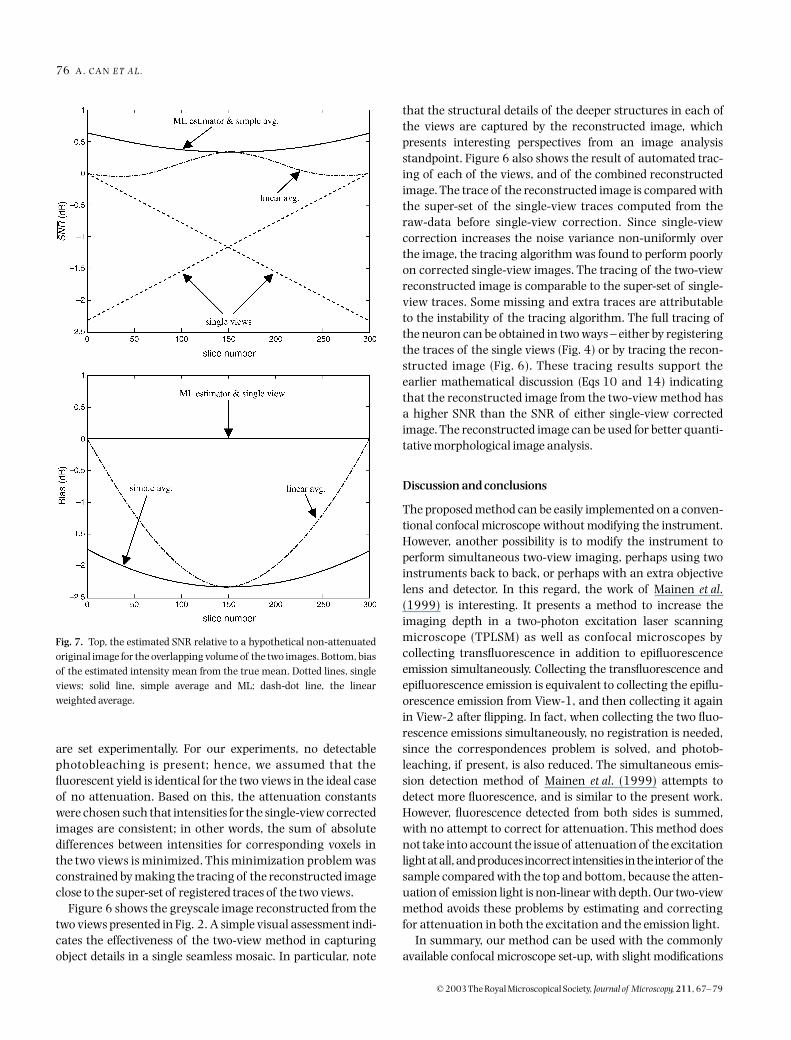
cal non-attenuated original image as a function of depth forthe different methods described above is plotted in Fig. 7. Thefigure also shows the bias of the estimated intensity meanfrom the true mean. The two-view reconstructions show asignificant improvement in the SNR compared to the singleviews, and work for all values of the attenuation constant.Using the ML or the average of the two views for reconstruc-tion produces the maximum gain in the SNR. However, thesimple average reconstruction is biased while the ML estima-tor is not. Linear weighted average produces suboptimal SNRgain, whereas it is less biased compared to the simple average.Single view correction is not biased, but it does not produceany SNR gain.

Experimental results

The flipped images of Fig. 2 show the effects of depth-dependentsignal attenuation on 3D image content. The projectionsof the first image (view-1) are presented in the left-hand col-umn and the second or flipped images (view-2) are presentedin the right-hand column. As shown, the images are not yetregistered. By examining the upper pair of images (the x–yprojection) it is easy to find dendrites in one image that are lessintense or even missing in the other image. The x–z and y–zimages show a very different distribution of dendrites in thez-direction between the two images.

Figure 4 shows the result of applying our tracing algo-rithms to the individual images of Fig. 2. Note that the traceson the right-hand side of Fig. 4 are flipped for clarity. The den-drites that are present in one view but missing in the other areobvious by this display method. The two-view image data canbe registered in 3D space by registering the individual traces.Figure 5 is the result of montaging the two tracing results ofFig. 4 into a single 3D image. The two individual traces arecolour-coded red and blue. Regions of correspondence betweenthe two traces are shown in green. It is easy to see in the x–zprojection which dendrites appeared in one image and whichappeared in the other. The blue dendrites were clearly the onescloser to the objective lens when imaged from the blue direc-tion and the reverse is clearly true for the red ones.

The result of attenuation correction in single-view images isshown in Fig. 3. In these images the depth-dependent signalattenuation is corrected for each of the two views of Fig. 2. Thedendrite intensities are more consistent as a function ofthe z-dimension. Attenuation constants through somal and

I( ) ( ) ( )

( )

( )

.xx x

x x

=+ ′

+′

I I

C C

1 2

1 2

1 1

I( ) xE Î[ ( )] ( )I x x= SNR

SNR SNRC C

( )

( )

.= +′

1 1

1 2x x

SNR

IAvg

I I( )

( ) ( ).x

x x=

+ ′1 2

2

EI

C CAvg[ ( )] ˆ( )

( )

( )I x

xx x

= +′

2

1 1

1 2

I( ) ( ) ( )x x x≈ C I1 1

I( ) ( )( ) ( )

.x xx x

=+ ′

CI I1 2

2

EI

D

D z

C

z

CLA[ ( )] ˆ( )

( )

( ),I x

xx x

=−

+′

1 2

SNR

SNR

D zC

zC

D zC

zC

( )

( )

( )( )

( )

=

− +′

− +′

1 2

2

1

2

2

x x

x x

T WO - V I E W C O N F O CA L I M AG E AT T E N UAT I O N C O R R E C T I O N 75

© 2003 The Royal Microscopical Society, Journal of Microscopy, 211, 67–79

non-somal profiles are also presented in Fig. 3 (solid and bro-ken lines, respectively). It is clear that in the major part of theimage, the attenuation is dominated by spherical aberration,which appears as a 1D exponential function. However, scat-

tering and absorption effects appear as a ‘bump’ in the profilethrough the soma, where the dye concentration is higher.

Visser et al. (1991) described a method to estimate theattenuation constants. In our implementation, those constants

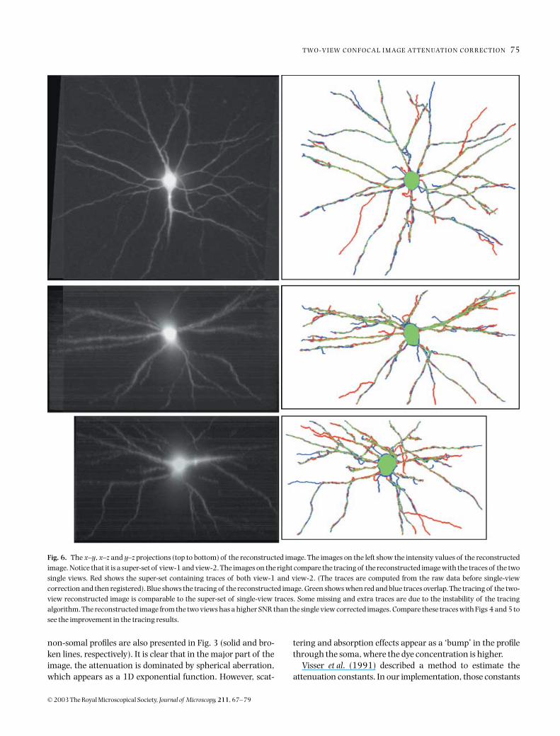
Fig. 6. The x–y, x–z and y–z projections (top to bottom) of the reconstructed image. The images on the left show the intensity values of the reconstructedimage. Notice that it is a super-set of view-1 and view-2. The images on the right compare the tracing of the reconstructed image with the traces of the twosingle views. Red shows the super-set containing traces of both view-1 and view-2. (The traces are computed from the raw data before single-viewcorrection and then registered). Blue shows the tracing of the reconstructed image. Green shows when red and blue traces overlap. The tracing of the two-view reconstructed image is comparable to the super-set of single-view traces. Some missing and extra traces are due to the instability of the tracingalgorithm. The reconstructed image from the two views has a higher SNR than the single view corrected images. Compare these traces with Figs 4 and 5 tosee the improvement in the tracing results.

76 A . CA N E T A L .

© 2003 The Royal Microscopical Society, Journal of Microscopy, 211, 67–79

are set experimentally. For our experiments, no detectablephotobleaching is present; hence, we assumed that thefluorescent yield is identical for the two views in the ideal caseof no attenuation. Based on this, the attenuation constantswere chosen such that intensities for the single-view correctedimages are consistent; in other words, the sum of absolutedifferences between intensities for corresponding voxels inthe two views is minimized. This minimization problem wasconstrained by making the tracing of the reconstructed imageclose to the super-set of registered traces of the two views.

Figure 6 shows the greyscale image reconstructed from thetwo views presented in Fig. 2. A simple visual assessment indi-cates the effectiveness of the two-view method in capturingobject details in a single seamless mosaic. In particular, note

that the structural details of the deeper structures in each ofthe views are captured by the reconstructed image, whichpresents interesting perspectives from an image analysisstandpoint. Figure 6 also shows the result of automated trac-ing of each of the views, and of the combined reconstructedimage. The trace of the reconstructed image is compared withthe super-set of the single-view traces computed from theraw-data before single-view correction. Since single-viewcorrection increases the noise variance non-uniformly overthe image, the tracing algorithm was found to perform poorlyon corrected single-view images. The tracing of the two-viewreconstructed image is comparable to the super-set of single-view traces. Some missing and extra traces are attributableto the instability of the tracing algorithm. The full tracing ofthe neuron can be obtained in two ways – either by registeringthe traces of the single views (Fig. 4) or by tracing the recon-structed image (Fig. 6). These tracing results support theearlier mathematical discussion (Eqs 10 and 14) indicatingthat the reconstructed image from the two-view method hasa higher SNR than the SNR of either single-view correctedimage. The reconstructed image can be used for better quanti-tative morphological image analysis.

Discussion and conclusions

The proposed method can be easily implemented on a conven-tional confocal microscope without modifying the instrument.However, another possibility is to modify the instrument toperform simultaneous two-view imaging, perhaps using twoinstruments back to back, or perhaps with an extra objectivelens and detector. In this regard, the work of Mainen et al.(1999) is interesting. It presents a method to increase theimaging depth in a two-photon excitation laser scanningmicroscope (TPLSM) as well as confocal microscopes bycollecting transfluorescence in addition to epifluorescenceemission simultaneously. Collecting the transfluorescence andepifluorescence emission is equivalent to collecting the epiflu-orescence emission from View-1, and then collecting it againin View-2 after flipping. In fact, when collecting the two fluo-rescence emissions simultaneously, no registration is needed,since the correspondences problem is solved, and photob-leaching, if present, is also reduced. The simultaneous emis-sion detection method of Mainen et al. (1999) attempts todetect more fluorescence, and is similar to the present work.However, fluorescence detected from both sides is summed,with no attempt to correct for attenuation. This method doesnot take into account the issue of attenuation of the excitationlight at all, and produces incorrect intensities in the interior of thesample compared with the top and bottom, because the atten-uation of emission light is non-linear with depth. Our two-viewmethod avoids these problems by estimating and correctingfor attenuation in both the excitation and the emission light.

In summary, our method can be used with the commonlyavailable confocal microscope set-up, with slight modifications

Fig. 7. Top, the estimated SNR relative to a hypothetical non-attenuatedoriginal image for the overlapping volume of the two images. Bottom, biasof the estimated intensity mean from the true mean. Dotted lines, singleviews; solid line, simple average and ML; dash-dot line, the linearweighted average.

T WO - V I E W C O N F O CA L I M AG E AT T E N UAT I O N C O R R E C T I O N 77

© 2003 The Royal Microscopical Society, Journal of Microscopy, 211, 67–79

only in the specimen preparation, while the simultaneousemission detection method requires additional set-up for theconfocal microscope used. In fact, we expect our method towork with multiphoton microscopes as well, even thoughthe experiments remain to be performed. Importantly, ourmethod yields a real improvement in the SNR, as well asenhanced imaging depth, and was shown to be applica-ble to regions with relatively low fluorochrome density (smalldendrites) and with very high fluorochrome density (somas).

Acknowledgements

This work was supported in part by CenSSIS, the Center forSubsurface Sensing and Imaging Systems, under the Engi-neering Research Centers Program of the National ScienceFoundation (Award Number EEC-9986821). We are gratefulto Dr Khalid Al-Kofahi for providing the automated algo-rithms for tracing the neurons, and to Dr Christopher Pacefor preparing the filled neuron samples that were used in thisstudy. Finally, we are grateful to the anonymous refereeswhose comments greatly enhanced this paper.

References

Adiga, U.P.S. & Chaudhuri, B.B. (2001) Some efficient methods to correctconfocal images for easy interpretation. Micron, 32, 363–370.

Al-Kofahi, O., Can, A., Lasek, S., Szarowski, D.H., Turner, J.N. & Roysam, B.(2003) Algorithm for 3-D registration of neuronal images acquired byconfocal scanning laser microscopy. J. Microsc. 211, 000–000.

Al-Kofahi, K., Lasek, S., Szarowski, D., Pace, C., Nagy, G., Turner, J.N. &Roysam, B. (2002) Rapid automated three-dimensional tracing ofneurons from confocal image stacks. IEEE Transactions InformationTechnol. Biomedicine, 6, 171–187.

Can, A., Lasek, S., Szarowski, D.H., Turner, J.N. & Roysam, B. (2000)A robust two-view method for increasing the imaging depth andcorrecting for signal attenuation in confocal microscope images. Proc.Microsc. Microanal. 6, 818–819.

Carlsson, K. (1991) The influence of specimen refractive index, detectorsignal integration, and non-uniform scan speed on the imagingproperties in confocal microscopy. J. Microsc. 163, 2, 167–178.

Cogswell, C.J., Larkin, K.G. & Klemm, H.U. (1996) Fluorescence micro-tomography: multi-angle image acquisition and 3D digital reconstruc-tion. SPIE, 2655, 109–115.

Diaspro, A. (2002) Confocal and Two-Photon Microscopy Foundations,Applications, and Advances. Wiley-Liss, Inc, New York.

Flock, S.T., Jacques, S.L., Wilson, B.C., Star, W.M. & van Gemert, M.J.C.(1992) Optical properties of intralipid: a phantom medium for lightpropagation studies. Lasers Surg. Med. 12, 510–519.

Frank, J. (2001) Cryo-electron microscopy as an investigative tool: theribosome as an example. Bioessays, 23, 725–732.

de Grauw, C.J., Vroom, J.M., van der Voort, H.T. & Gerritsen, H.C. (1999)Imaging Properties in two-photon excitation microscopy and effects

of refractive-index mismatch in thick specimens. Appl. Opt. 38, 5995–6003.

Heintzmann, R., Kreth, G. & Cremer, C. (2000) Reconstruction of axialtomographic high resolution data from confocal fluorescence micros-copy: a method for improving 3D FISH images. Anal. Cell. Pathol. 20, 7–15.

Hell, S., Reiner, G., Cremer, C. & Stelzer, E.H.K. (1993) Aberrations inconfocal fluorescence microscopy induced by mismatches in refractiveindex. J. Microsc. 169, 391–405.

Jacobsen, H., Hanninen, P., Soini, E. & Hell, S.W. (1994) Refractive-index-induced aberrations in two-photon confocal microscopy. J. Microsc.176, 226–230.

Liljeborg, A., Czader, M. & Porwit, A. (1995) A method to compensatefor light attenuation with depth in three-dimensional DNA imagecytometry using confocal scanning laser microscope. J. Microsc. 177,108–114.

Mainen, Z.F., Maletic, S.M., Shi. S.H., Hayashi, Y., Malinow, R. & Svoboda, K.(1999) Two-photon imaging in living brain slices. Methods: a Companionto. Meth. Enzymol. 18, 231–239.

Margadant, F., Leemann, T. & Niederer, P. (1996) A precise light attenua-tion correction for confocal scanning microscopy with O (N4/3) comput-ing time and O (N) memory requirements for N voxels. J. Microsc. 182,121–132.

Mastronarde, D.N. (1997) Dual Axis tomography: an approach withalignment methods that preserve resolution. J. Struct. Biol. 120,343–352.

Nagelhus, T.A., Slupphaug, G., Krokan, H.E. & Lindmo, T. (1996) Fadingcorrection for fluorescence quantitation in confocal microscopy.Cytometry, 23, 187–195.

Pawley, J. (ed.) (1995) Handbook of Confocal Microscopy. Plenum Press,New York.

Rigaut, J.P. & Vassy, J. (1991) High-resolution three-dimensional imagesfrom confocal scanning laser microscopy. Anal. Quantitative Cytol.Histol. 13, 223–232.

Roerdink, J.B.T.M. (1994) FFT-based methods for nonlinear imagerestoration in confocal microscopy. J. Mathemat. Imaging Vision, 4, 199–207.

Roerdink, J.B.T.M. & Bakker, M. (1993) An FFT-based method for attenu-ation correction in fluorescence confocal microscopy. J. Microsc. 169,3–14.

Roysam, B., Bhattacharjya, A.K., Srinivas, C. & Turner, J.N. (1992)Unsupervised noise removal algorithms for 3-D confocal fluorescencemicroscopy. Micron Microsc. Acta, 23, 447–461.

Shaw, P.J. (1990) Three-dimensional optical microscopy using tiltedviews. J. Microsc. 158, 165–172.

Shaw, P.J., Agard, D.A., Hiraoko, Y. & Sedat, J.W. (1989) Tilted viewreconstruction in optical microscopy, three-dimensional reconstruc-tion of Drosophila melanogaster embryo nuclei. J. Microsc. 55, 101–110.

Strasters, K.C., Van der Voort, H.T.M., Geusebroek, J.M. & Smeulders, A.W.M.(1994) Fast attenuation correction in fluorescence confocal imaging:a recursive approach. Bioimaging, 2, 78–92.

Visser, T.D., Groen, F.C.A. & Brakenhoff, G.J. (1991) Absorption andscattering correction in fluorescence confocal microscopy. J. Microsc.163, 189–200.

78 A . CA N E T A L .

© 2003 The Royal Microscopical Society, Journal of Microscopy, 211, 67–79

Appendix A: scattering, refraction and absorption

If the focal plane is deep inside the sample, the amount ofscattered light (excitation and fluorescent) increases, as wellas the PSF size, reducing the fluorescent yield as a result.

The equation that describes the signal attenuation on theway to and from the focus point is given by Diaspro (2002) andFlock et al. (1992):

(A1)

where I(z,λ) is the collected light, which is a function of thefocal position (see Fig. 1) and the wavelength, λ, used.αexc = αs,exc + αa,exc is the attenuation coefficient for the excita-tion light, αs,exc for scattering and refraction, and αa,exc forabsorption, of the excitation light. αem = αs,em is the attenuationcoefficient for the emitted light, which reflects attenuationdue to scattering and refraction of emitted light only, sincereabsorption of emitted photons is neglected (Diaspro, 2002).For small-NA objectives, the distance z is approximately equalto the distance from the top cover slip (with respect to theobjective) to the focal position. However, for large-NA objec-tives used in our experiments (NA = 1.15), Eq. (A1) definedabove should be integrated over the light cone shown in Fig. 1.When the spherical aberration is significant, as in our mis-matched system, only the low-NA rays will contribute to theimage, all higher-angle rays being deflected far from the focus bythe aberrations. Hence, the semi-aperture angle, ω, used shouldbe smaller than the actual ω dictated by the objective used.

The excitation light (forward direction) and the emittedlight (backward direction) can be integrated separately to sim-plify the computations. To facilitate the discussion, we attacha Cartesian coordinate system to the specimen x = (x,y,z)T,where x and y show the coordinates on an observed opticalsection, and z shows the depth (Fig. 1). Here we assume thatthe z-axis is aligned along the optical axis of the microscope.Let (r,θ,φ) be the representation of a point within the speci-men, expressed in spherical coordinates. If a ray with angles θand φ is traveling through a homogeneous medium, the inten-sity at x = (x,y,z)T will be

(A2)

Here z/cos θ is the length of the path that the ray travels. Fora non-homogeneous medium, the extinction coefficient willbe different at each point in space; hence the final intensity canbe written more generally as

(A3)

The objective lens of the system converts this monochromaticplane wave into a converging spherical wave, bounded by

the semi-aperture angle ω, with radius R. In the hypotheticalcase of zero attenuation, the total excitation intensity iscalculated as:

(A4)

where Iin is the intensity of light per unit area, and cos θ is dueto the convergence of the uniform bundle into a spherical wave.

Scattering and refraction can be broken into two compo-nents: those that are inherent to the sample itself, and are nota function of the fluorophore distribution, and those that areproportional to the fluorophore distribution. Both compo-nents have the same effect of scattering the light and increas-ing the PSF size, and both are modelled by exponentialattenuation in our experiments. The first component is a func-tion of path travelled only (see Eq. A2), and the attenuationcoefficients are constants (not a function of fluorophore distri-bution). The second component is proportional to the fluoro-phore density along the path travelled, and is described byEq. (A3).

As a result, we have

(A5)

αs,exc and αs,em represent the extinction coefficients for scatter-ing and refraction components for the excitation and emittedlights, respectively. The subindex ‘smpl’ represents the sampleinherent components, which depend on the length of the lightpath only, while the subindex ‘flor’ represents the componentsproportional to the fluorphore distribution. Hence, the totalexcitation intensity for a non-homogeneous medium can beexpressed as

(A6)

We assume that this excitation light is absorbed by thefluorochrome, and fluorescence is emitted proportional tothe fluorochrome density and the incident light intensity. If therelationship is different, the equation below can be amendedappropriately. The emitted fluorescence light intensity is

If (x) = cpρ(x)Ie(x), (A7)

where cp is a factor related to the quantum efficiency of thefluorochrome. Although cp is a function of time and space dueto photobleaching, for our specimen preparation and imagingconditions, however, we can demonstrate that there is nosignificant photobleaching for the two views.

I z I z I e eexc emz zexc em( , ) exp[ ( ) ] λ α α α α= − + = − −

0 0

I I e I en

zz

z

exc

exc( ) .cos /cosx = =

− ′−

0 00

� αθ α θ

d

I I en

z

z

exc

( ) .( )

cosx

x

=− ′′

00

�αθ

d

I I R I Rin in0

0 0

2

2 2 2 cos sin sin ,= =

ω π

θ θ φ θ π ω�� d d

α α αα α α

s exc s exc smpl s exc flor

s em s em smpl s em flor

, , , , ,

, , , , ,

= += +

I I R

z

e in

z

s exc flor s exc smpl a exc

( ) cos sin

exp( ) ( ), , , , ,

x

x x

=

−′ + + ′

′

0 0

2

2

0

ω π

θ θ

α α αθ

φ θ

��

� cosd d d

T WO - V I E W C O N F O CA L I M AG E AT T E N UAT I O N C O R R E C T I O N 79

© 2003 The Royal Microscopical Society, Journal of Microscopy, 211, 67–79

The emitted light travels back along the same path as theincoming radiation and the detected light is then

(A8)

which is similar to Eq. (A6) except that there is no cos θfactor inside the integration because of the assumption ofisotropic emission. The extinction coefficients for the neu-ron images can be approximated as a linear function of thefluorochrome density plus the sample inherent components,under the assumption that the extinction is small (Visser et al.,1991). Substituting Eqs (A6) and (A7) into Eq. (A8) yields

(A9)

where the factors αexc(x) and αem(x) are described in Eqs (A1)and (A5). If there is no attenuation, then αexc(x) = αem(x) = 0,and the above equation reduces to

(A10)

Î(x) is the expected light intensity to be observed under noattenuation, which is simply the fluorochrome density multipliedby constants.

Glossary of mathematical terms

Î(x) Original intensity, i.e. the expected intensity to beobserved under no-attenuation condition.

I1(x), I2(x) Observed attenuated intensity in the first andsecond views.

C1(2)(x) Computed correction coefficient from the observedintensity value in the first (second) view.

I (x) Estimated intensity value from the two views.

II

zf

z

s em flor s em smpl( ) ( )

sin exp( ) , , , ,x

x x= −

′ +′

4

0 0

2

0π

θα α

θφ θ

ω π

� � � cosd d d

Ic I R

e

e

p inz

z

z

em

z

exc

( ) ( )

sin

cos sin ,

( )

( )

x =− ′

′

− ′′

2

0 0

2

0 0

2

40

0

ρπ

θ φ θ

θ θ φ θ

ω π αθ

ω π αθ

xx

x

��

��

�

�

cosd

cosd

d d

d d

Îc I Rp in( )

( ) sin ( cos ).x

x= −

22

42 1

ρπ

π ω π ω