
Development of confocal microscope for polarimetry of ...
155
HAL Id: tel-03471441 https://tel.archives-ouvertes.fr/tel-03471441 Submitted on 8 Dec 2021 HAL is a multi-disciplinary open access archive for the deposit and dissemination of sci- entific research documents, whether they are pub- lished or not. The documents may come from teaching and research institutions in France or abroad, or from public or private research centers. L’archive ouverte pluridisciplinaire HAL, est destinée au dépôt et à la diffusion de documents scientifiques de niveau recherche, publiés ou non, émanant des établissements d’enseignement et de recherche français ou étrangers, des laboratoires publics ou privés. Development of confocal microscope for polarimetry of semiconductor nano-structures Meryem Benelajla To cite this version: Meryem Benelajla. Development of confocal microscope for polarimetry of semiconductor nano- structures. Physics [physics]. INSA de Toulouse, 2020. English. NNT : 2020ISAT0028. tel- 03471441
-
Upload
khangminh22 -
Category
Documents
-
view
3 -
download
0
Transcript of Development of confocal microscope for polarimetry of ...

HAL Id: tel-03471441https://tel.archives-ouvertes.fr/tel-03471441
Submitted on 8 Dec 2021
HAL is a multi-disciplinary open accessarchive for the deposit and dissemination of sci-entific research documents, whether they are pub-lished or not. The documents may come fromteaching and research institutions in France orabroad, or from public or private research centers.
L’archive ouverte pluridisciplinaire HAL, estdestinée au dépôt et à la diffusion de documentsscientifiques de niveau recherche, publiés ou non,émanant des établissements d’enseignement et derecherche français ou étrangers, des laboratoirespublics ou privés.
Development of confocal microscope for polarimetry ofsemiconductor nano-structures
Meryem Benelajla
To cite this version:Meryem Benelajla. Development of confocal microscope for polarimetry of semiconductor nano-structures. Physics [physics]. INSA de Toulouse, 2020. English. �NNT : 2020ISAT0028�. �tel-03471441�


Acknowledgements
”Ce que l’on conçoit bien s’énonce clairement,et les mots pour le dire arrivent aisément.” Nicolas Boileau-Despréaux
It is my pleasure to acknowledge the members of my thesis committee: Jean-Jacques Greffet, Olivier Krebs, Isabelle Robert-Philip, Vincent Paillard, KhaledKarrai, Bernhard Urbaszek for generously offering their time, support, guidanceand good will throughout the preparation and review of this document.
This journey would not have been possible without the support of my family,professors and mentors, and friends. I spend in total three years at the companyattocube systems, including my secondments at the Laboratoire de Physique etChimie des Nano-Objets. Those years have been rich in scientific achievements. Ihad the chance to cross the way of many interesting and exciting people withoutwhom this thesis would not have been possible.
Most of all, I would like to express my gratitude to my supervisor at thecompany attocube; Prof. Khaled Karrai for his continuous support, patience, mo-tivation, enthusiasm, and immense knowledge. Your insightful feedback duringthe planning and development of this research work pushed me to sharpen mythinking and brought my work to a higher level. Your willingness to help at anytime has been very much appreciated. Thank you for all the opportunities youprovides me and all the work methods I learned at your contact during those3 years. I will keep a very good memory of that workshop on Lake Achenseein Austrian Alps. I very much enjoyed walking in the panoramic view of thelake and mountains and breathe in the fresh, clean air. Encore une fois, mercibeaucoup Khaled!
3

My grateful thanks are also extended to my supervisor at the University ofToulouse; Prof. Bernhard Urbaszek who has provided me with extensive personaland professional guidance throughout the duration of my Ph.D. thesis. Yourvaluable advice, ingenious recommendations and profound belief in my workwere a key element that allows me to achieve a successful thesis with a manyscientific results and a lot of new experiences. I had a wonderful memorabletime in Toulouse that I will never forget. I enjoyed our walking tour togetherwith Shivangi very much and all the tasty local food especially the HomemadeWaffles with Salted Caramel Sauce. Ein letzes mal, vielen dank Bernhard!
My sincere thanks to R. Warburton, M. Kroner, L. Novotny, Alexander Högele,Massimo Gurioli, Elena Kammann and C. Schaefermeier for useful discussionsand valuable suggestions. This research project has received funding from theEuropean Union’s Horizon 2020 research and innovation programme under theMarie Skłodowska-Curie grant agreement No721394 ITN 4PHOTON. Thank you4PHOTON team for the wonderful meetings and workshops. It was a perfectmix of topics, people, science and social gathering!
My special gratitude to many people I met, worked with; who helped mein different ways throughout my studies. I tried to list them all but I probablyforget some, thank you, everyone, and please accept my apologies!
• attocube colleagues: E. Kammann, C. DalSavio, C. Schaefermeier, J. Lind-lau, H. Thierschmann, S. Vadia, C. K. V. Grundherr, P. Kuehnemann, G.Wuest, K. Grafenstein, S. Muller, T. Maier, P. Leubner, P. Kellner, I. Park,T. Rind, O. Seidel, A. Schmidt, M. Matheus, T. Lesnicar, N. Grill, K. Hoe-fling, Y. Heubeck, L. Zierl, A. Reuter, V. Dahlmeier, F. Otto, K. Bittner, K.Simi, B. Sipos, V. Kuemmerling, G. Schindler, S. Oberbauer, M. Bacani, T.Linderberg, V. Gentz, E. Trommer, M. Potsi, A. Piccolo, F. Valmorra.
• LPCNO colleagues: S. Shree, B. Han, X. Marie, C. Robert, T. Amand,D. Lagarde, H. Fang, G. Wang, E. Courtade, I. Paradeisanos, M. Manca,P. Renucci, L. Lombez, A. Balocchi, H. Carrere, L. Ren, J. Rajagopal, H.Tornatzky, J-F. Leherissier, B. Lassagne, T. Blon and É. Palleau.
• 4PHOTON colleagues: S. Stanguinetti, S. Bietti, S. Soubes, R. Waburton,L. Zhai, A. Tartakovskii, A. Fognini, A. Guardiani, A. Tuktamyshev, B.Giorgios, D. Toliopoulos, G. Bester, G. Pirard, H. Cristian, H. Liu, J. Muller,L. Ranasinghe, M. Abbarchi, M. Gurioli, M. Flatte, M. Glazov, P. Sheard, P.M. Koenraad, P. Zotev, P. A. Wronski, S. Dorenbos, S. Hofling, V. Zwiller,W. Hansen, A. Ludwig, D. Ritchie, R. S. R. Gajjela, A. Cruz, A. Shields, R.M. Stevenson.
M�e�r�y�e�m�
4


Abstract
Confocal microscopy is an essential imaging tool for biological systems, in solid-state physics and nano-photonics. Using confocal microscopes allows performingresonant fluorescence experiments, where the emitted light has the same wave-length as the excitation laser. Theses challenging experiments are carried outunder linear cross-polarization conditions, rejecting laser light from the detector.In this work, we uncover for the first time the physical mechanisms that are atthe origin of the yet unexplained high polarization rejection ratio which makesthe resonant fluorescence measurements possible. We show in both experimentand theory that the use of a reflecting surface (i.e. the beam-splitter and mirrors)placed between two polarizers in combination with a confocal arrangementexplains the giant cross-polarization extinction ratio of 108 and beyond. We mapthe modal transformation of the polarized optical Gaussian beam. We find anintensity "hole" in the reflected beam under cross-polarization conditions. Weinterpret this as a manifestation of the Imbert-Fedorov effect. We confirm theseexperimental findings for a large variety of commercially available mirrors andpolarizers, allowing their practical implementation in many experiments.
Learning from this first part, we moved our exploration to a more funda-mental aspect of optics in order to test the predictive power of the model. TheImbert-Fedorov shift, also known as "spin-Hall effect of light", was first measuredfor a laser beam of circularly polarized light in a glass prism under total internalreflectivity condition. Depending on the chirality of its circular polarization,the trajectory of a circularly polarized beam will shift above or below the planeof reflectivity when reflected off a surface. This shift is due to spin-orbit cou-pling of light upon each reflection and is normally very small, typically, severalorder of magnitudes smaller than the photon wavelength. For this reason, ithas previously required using complex detection schemes limiting detailed ex-perimental investigations. Here, we report about a novel method to measureand map the Imbert-Fedorov shift based on a dark-field cross-polarization tech-nique in a confocal arrangement. In our proposed dark-field configuration incircular polarization, the majority photons reflected off a silver surface that arenot contributing to the shift are filtered-out. The minority photons possess theproper chirality for spin-orbit coupling enabling this way the magnification ofthe Imbert-Fedorov shift by several orders of magnitudes. We verified that theout of plane of incidence shift measured this way is a direct consequence of theconservation of total angular momentum. Building on our detailed model forGaussian beams derived for the first part of this work we have verified quanti-
5

tatively experimentally that the shift increases significantly when decreasingthe angle of incidence, this, to the best of our knowledge, is a novel regime thatwas not explored previously. The analytical model show an excellent agreementwith our measurements performed on high reflectivity metals such as silver. Inparticular, the model reveals clearly a regime of lower angle of incidence belowwhich the simplistic approach of quasi plane wave would lead to an unphysicaldivergence of the shift at vanishing angles. In such a low angle regime, our modeleliminates this shift divergence and predicts instead a modal transformation ofthe reflected minority photons to the next higher Hermite-Gaussian mode in away very similar to that explored in the first part of this work. First data indicatethe transition into such a regime.
Finally, this work opens the way to methodical design of sensitive laserresonant-fluorescence microscopes with extreme background extinction, for abroad range of applications in quantum optics and solid-state physics. The newmethods developed here can also be applied for measuring material opticalproperties.
6

Résumé
La microscopie confocale est un outil d’imagerie essentiel pour les systèmesbiologiques, en physique du solide et en nano-photonique. L’utilisation d’untel microscope permet de réaliser des mesures de fluorescence résonante, où lalumière émise a la même longueur d’onde que la source. Ces mesures difficilessont menées en condition de polarisation croisée linéaire, rejetant la lumièrelaser du détecteur. Dans ce travail, nous expliquons pour la première fois lesmécanismes physiques du taux de rejet de polarisation élevé encore inexpliquéqui rend possible les mesures de fluorescence résonante. Nous montrons à la foisdans l’expérience et la théorie que l’utilisation d’une surface réfléchissante (leséparateur de faisceau et les miroirs) placée entre deux polariseurs en combinai-son avec un arrangement confocal explique le taux d’extinction géant de 108 etau-delà. Nous illustrons la transformation modale du faisceau gaussien polarisé.Nous trouvons un «trou» d’intensité dans le faisceau réfléchi dans ces condi-tions. Nous interprétons cela comme une manifestation de l’effet Imbert-Fedorov.Nous confirmons ces résultats pour une grande variété de miroirs et polariseursdisponibles dans le commerce, permettant leur mise en œuvre pratique dans denombreuses expériences.
Par la suite, nous avons exploré un aspect plus fondamental de l’optique pourtester notre modèle. Le décalage d’Imbert-Fedorov, également connu commel’«effet de spin-hall de la lumière», a d’abord été mesuré pour un faisceau laserde lumière polarisée circulairement dans un prisme de verre en condition deréflectivité interne totale. En fonction de la chiralité de sa polarisation, la trajec-toire d’un faisceau polarisé circulairement se déplacera au-dessus ou au-dessousdu plan de réflectivité lorsqu’il est réfléchi sur une surface. Ce décalage est dûau couplage spin-orbite de la lumière à chaque réflexion et est normalement trèspetit, typiquement, plusieurs ordres de grandeur plus petits que la longueurd’onde du photon. Pour cette raison, il était auparavant nécessaire d’utiliser desschémas de détection complexes limitant les investigations expérimentales. Ici,nous rapportons une nouvelle méthode pour mesurer et illustrer ce décalagebasée sur une technique de polarisation croisée en champ sombre dans un ar-rangement confocal. Dans cette configuration, la majorité des photons réfléchispar le miroir qui ne contribuent pas au décalage sont filtrés. Les photons minori-taires possèdent la chiralité appropriée pour le couplage spin-orbite permettantainsi le grossissement du décalage de plusieurs ordres de grandeur. Nous avonsvérifié que le décalage hors plan d’incidence mesuré de cette manière est uneconséquence directe de la conservation du moment cinétique total. En se basant
7

sur notre modèle dérivé en première partie, nous avons vérifié expérimentale-ment que le décalage augmente de manière significative en diminuant l’angled’incidence, ceci, à notre connaissance, est un nouveau régime qui n’a pas étéexploré. Le modèle montre un excellent accord avec nos mesures effectuéessur un mirror métallique. En particulier, le modèle révèle un régime d’angled’incidence inférieur en dessous duquel l’approche simpliste de la quasi-ondeplane mène à une divergence non physique du décalage. Dans un tel régime,notre modèle élimine cette divergence de décalage et prédit une transforma-tion modale des photons minoritaires réfléchis vers le mode Hermite-Gaussiensupérieur suivant d’une manière similaire à celle explorée dans la première par-tie de ce travail. Les premières données indiquent la transition vers un tel régime.
Enfin, ces travaux ouvrent la voie à la conception méthodique de microscopesà fluorescence résonante laser sensibles à extinction de fond extrême, pour unelarge gamme d’applications en optique quantique et en physique du solide. Lesméthodes développées ici peuvent également être appliquées pour mesurer lespropriétés optiques des matériaux.
8


Contents
Acknowledgements 3
Abstract 5
Résumé 7
1 Resonant spectroscopy: the motivation to go beyond instrument’s limit 131.1 Introduction . . . . . . . . . . . . . . . . . . . . . . . . . . . . . . 131.2 Scope of the thesis . . . . . . . . . . . . . . . . . . . . . . . . . . . 15
2 Confocal microscope setup with polarization extinction 172.1 Confocal microscope for cryogenic spectroscopy . . . . . . . . . 18
2.1.1 Optical design . . . . . . . . . . . . . . . . . . . . . . . . . 182.1.2 Application to nanoscale spectroscopy . . . . . . . . . . . 202.1.3 Conclusion . . . . . . . . . . . . . . . . . . . . . . . . . . . 20
2.2 Confocal arrangement for cross-polarization extinction . . . . . 212.2.1 Confocal setup design . . . . . . . . . . . . . . . . . . . . 212.2.2 Confocal setup concept . . . . . . . . . . . . . . . . . . . 222.2.3 Confocal setup realization . . . . . . . . . . . . . . . . . . 232.2.4 Confocal setup alignment . . . . . . . . . . . . . . . . . . 252.2.5 Conclusion . . . . . . . . . . . . . . . . . . . . . . . . . . . 25
3 The physical origins of cancellation of polarization leakage 273.1 Polarization leakage equation . . . . . . . . . . . . . . . . . . . . 273.2 Material and angular dependency . . . . . . . . . . . . . . . . . . 293.3 Wavelength dependency . . . . . . . . . . . . . . . . . . . . . . . 313.4 Conclusion . . . . . . . . . . . . . . . . . . . . . . . . . . . . . . . 31
4 Modal transformation of a reflected polarized Gaussian beam 334.1 Experimental modal analysis of beam reflectivity . . . . . . . . . 33
4.1.1 Experimental details . . . . . . . . . . . . . . . . . . . . . 334.1.2 Confocal imaging of Imbert-Fedorov modes . . . . . . . . 34
4.2 Theoretical modal analysis of beam reflectivity . . . . . . . . . . 374.2.1 Mirror transfer matrix in angular domain . . . . . . . . . 374.2.2 Mirror transfer matrix in space domain . . . . . . . . . . 404.2.3 Effect of confocal filtering . . . . . . . . . . . . . . . . . . 424.2.4 Understanding effect of metal mirrors reflectivity . . . . . 44
9

4.3 Observation on different materials . . . . . . . . . . . . . . . . . 464.4 Experimental limits, so far . . . . . . . . . . . . . . . . . . . . . . 50
5 Circular polarization basis: direct imaging of Imbert-Fedorov effectin confocal microscopy 555.1 Motivation . . . . . . . . . . . . . . . . . . . . . . . . . . . . . . . 555.2 Spin and angular momentum of a plane wave . . . . . . . . . . . 585.3 Confocal imaging of Imbert-Fedorov shift . . . . . . . . . . . . . 60
5.3.1 Experimental setup with circularly polarized light . . . . 605.3.2 Experimental results with circularly polarized light . . . 61
5.4 Measurements at different angles of incidence . . . . . . . . . . . 665.5 Imbert-Fedorov shift for a circularly polarized Gaussian beam . 695.6 Imbert-Fedorov shift without the use of polarization analyzer . 735.7 Remark . . . . . . . . . . . . . . . . . . . . . . . . . . . . . . . . . 775.8 Conclusion . . . . . . . . . . . . . . . . . . . . . . . . . . . . . . . 78
6 Summary and perspectives 79
Appendix A Supplementary information to chapter 3“The physical origins of cancellation of polarization leakage” 81A.1 Jones calculus . . . . . . . . . . . . . . . . . . . . . . . . . . . . . 81A.2 Expression of the electric field after the analyzer (equation (3.4)) 83A.3 Expression of the light intensity after the analyzer (equation (3.6)) 83A.4 Angular shift as a function of Fresnel reflection coefficients . . . 84A.5 Maximum acceptable limit of polarization leakage . . . . . . . . 87
Appendix B Supplementary information to chapter 4“Modal transformation of a reflected polarized Gaussian beam” 91B.1 Reflection matrix as a function of (u,v) (equation (4.3)) . . . . . 91B.2 Reflected field distribution in the (x,y) domain (equation (4.4)) . 94
B.2.1 p-polarization . . . . . . . . . . . . . . . . . . . . . . . . . 97B.2.2 s-polarization . . . . . . . . . . . . . . . . . . . . . . . . . 99
B.3 Reflection matrix as a function of (x,y) (equation (4.6)) . . . . . 100
Appendix C Supplementary information to chapter 4“Effect of confocal spatial filtering” 105C.1 Spatial filtering with a single mode fiber (equation (4.8)) . . . . 105C.2 Reflection matrix including confocal filtering (equation (4.9)) . . 107C.3 Reflected field distribution for p (or s) polarized beam . . . . . . 109
C.3.1 Expression of the electric field after the fiber . . . . . . . 109C.3.2 Intensity of the lobe maxima at cross-polarization (equa-
tion (4.12)) . . . . . . . . . . . . . . . . . . . . . . . . . . . 110
Appendix D Supplementary information to chapter 4“Integrated intensity without confocal filtering (equation (4.11))” 113
10

Appendix E Supplementary information to chapter 4“Polarization structure of higher-order Hermite-Gaussian laser beams”115E.1 Focusing of a Gaussian beam: solution as a function of u and v . 115E.2 Focusing of a Gaussian beam: solution as a function of x and y . 117E.3 Application to p- polarization (equation (4.13)) . . . . . . . . . . 119
Appendix F Supplementary information to chapter 5“Evaluation of the Fresnel coefficient in the limit of small angles ” 121
Appendix G Supplementary information to chapter 5“Jones Vectors and Matrices ” 123
Appendix H Supplementary information to all chapters“Gaussian beam propagation” 125
Appendix I Summary of the present manuscript in french 127I.1 Chapitre 1: Spectroscopie résonnante: la motivation d’aller au-
delà de la limite de l’instrument . . . . . . . . . . . . . . . . . . . 127I.2 Chapitre 2: Configuration confocal avec extinction de polarisation 129I.3 Chapitre 3: Les origines physiques de l’annulation de fuite de
polarisation . . . . . . . . . . . . . . . . . . . . . . . . . . . . . . . 134I.4 Chapitre 4: Transformation modale de la réflectivité d’un faisceau
Gaussien polarisé . . . . . . . . . . . . . . . . . . . . . . . . . . . 135I.5 Chapitre 5: Base de polarisation circulaire: directe imagerie de
l’effet Imbert-Fedorov avec la microscopie confocale . . . . . . . 141I.6 Chapitre 6: Conclusion et perspectives . . . . . . . . . . . . . . . 146
Bibliography 149
11


Chapter 1
Resonant spectroscopy: themotivation to go beyond
instrument’s limit
Adapted from [1]:Meryem Benelajla, Elena Kammann, Bernhard Urbaszek, and Khaled Karrai,”The physical origins of extreme cross-polarization extinction in confocal mi-croscopy”, arXiv:2004.13564 (2020).
1.1 Introduction
In optical spectroscopy experiments it is crucial to excite an emitter with a laservery close to its transition energy. Experiments under resonant excitation areessential for accessing the intrinsic optical and spin-polarization properties oflarge class of emitters [2–7]. Using linear cross-polarization in a confocal setuphas been successfully employed as a dark-field method to carry out resonantfluorescence experiments to suppress scattered laser light, with the added benefitof high spatial resolution [8,9]. Resonant fluorescence experiments allow crucialinsights into light-matter coupling, such as the interaction of a single photonemitter with its environment [10], with optical cavities [11] and also studyingsingle defects in atomically thin materials such as WSe2 [12]. Dark-field confocaltechniques allow developing single photon sources with high degrees of photonindistinguishability [13–15] and longer coherence [16]. In practice dark-fieldlaser suppression is not just a spectroscopy tool, it is also a key part of morematured quantum technology systems [17].
Despite many advances based on experiments in confocal microscopes withcross-polarization laser rejection, the physical mechanisms that make theseexperiments possible are not well understood, hampering further progress inthis field. The key figure of merit is the suppression of the excitation laserbackground by at least six orders of magnitude. Indeed a suppression by a factorof 108 [18] up to 1010 (this work) has been measured. But this is very surprisingas mirrors and beam-splitter in such a system reduce the theoretical extinction
13

Chapter 1 – Resonant spectroscopy: the motivation to go beyond instrument’slimit
limit to the 103 to 104 range.
Figure 1.1: taken from [18]. (a) Microscope setup for resonance fluorescenceexperiments on a single InGaAs quantum dot. (b) Sensitivity of the laser sup-pression to the quarter-wave plate angle. (c) Long-term behaviour. The opticaldensity (OD), defined as OD = −log(1/T ) with transmission T, is plotted as afunction of time. The microscope is stable over many hours with an OD > 6.8.
In this work we explain the physics behind the giant enhancement of theextinction ratio by up to seven orders of magnitude that make microscopy basedon dark-field laser suppression possible. The measurements of resonant fluores-cence are typically performed in an epifluorescence geometry [18], for whichlaser excitation and fluorescence collection are obtained through the same fo-cusing lens. This involves necessarily the use of a beam-splitter orienting theback-reflected light containing the fluorescence towards a detection channel asdepicted in Fig. 1.1. The back-reflected laser is suppressed by rotating a quarter-wave plate, switching between laser rejection maximally on and maximally off.The implementation of this scheme Fig. 1.1(a) demonstrated an impressivelyhigh suppression of laser excitation background in excess of a factor of 108
(Fig. 1.1. (b) and (c)) corresponding to an optical density OD=8. Fig. 1.1. (b)shows that this giant extinction depends on the quarter-wave plate angle anda change of only few mdeg can decrease the level of background rejection byone order of magnitude. In another words, this emphasizes the need for a mdegrotation resolution and an extreme control of polarization to be able to performa resonance fluorescence experiments on quantum emitters.
In our work we identify two key ingredients that explain the giant ampli-fication of the cross-polarization extinction ratio: (i) a reflecting surface (i.e.
14

Chapter 1 – Resonant spectroscopy: the motivation to go beyond instrument’slimit
the beam-splitter) placed between a polarizer and analyzer, and (ii) a confocalarrangement. We demonstrate giant extinction ratios in our experiments fordifferent mirrors (silver, gold, dielectric, beam-splitter cubes) and polarizers(Glan-Taylor, nanoparticle thin films). We demonstrate that behind this gen-eral observation lies the intriguing physics of the Imbert-Fedorov effect [19, 20],which deviates a reflected light beam depending on its polarization helicity.We discover that a confocal arrangement not only amplifies the visibility ofthe Imbert-Fedorov effect dramatically, taking it from the nanometer to themicrometer scale, but also exploits conveniently the symmetry of the newlyobserved Imbert-Fedorov modes to insure that the cross-polarized laser beam isnot coupled, explaining the near complete suppression of the laser backgroundsignal. In other words, we cannot treat the spatial (i.e. modal) and polarizationproperties of light separately in our dark-field confocal microscope analysis. Inaddition to new developments in dark-field microscopy our experiments providepowerful tools to understand spin-orbit coupling of light [21–23], in the broadercontext of topological photonics [22, 23].
In our work we setup a robust, highly reproducible experiment and derivea convenient classical formalism to investigate these remarkable effects at thecross roads of quantum optics and topological photonics.
1.2 Scope of the thesis
The thesis is structured as follows, in chapter 2 we introduce the confocal mi-croscope setup with polarization extinction, confocal microscope design forcryogenic spectroscopy is discussed in section 2.1, the simplified confocal ar-rangement for cross-polarization extinction measurement is described in section2.2. Cancellation of polarization leakage is measured and discussed in a firstsimplified model in chapter 3. The modal transformation of a reflected Gaussianbeam is analyzed in chapter 4. Direct imaging of the Imbert-Fedorov shift effectusing circular polarization state of light is presented in chapter 5.
15


Chapter 2
Confocal microscope setup withpolarization extinction
Adapted from [24]:Meryem Benelajla, Elena Kammann, Bernhard Urbaszek, and Khaled Karrai”Modal imaging of a laser Gaussian-beam reflected off a surface”,Proceedings Volume 11485, Reflection, Scattering, and Diffraction from SurfacesVII; 114850E (2020).
In this chapter we start by describing the attocube fiber-based confocalmicroscope instrument for nanoscale spectroscopy at cryogenic temperaturesand in high magnetic fields (section 2.1.1). As a demonstration of the microscopeperformance, applications in the spectroscopy of single quantum emitters arepresented in section 2.1.2. The confocal microscope presented in section 2.1is designed to obtain a high polarization extinction ratio with a convenientswitching between laser rejection maximally on and maximally off. Section 2.2describes the simplified confocal arrangement we used in order to focus on themost relevant physics leading to extreme laser rejection. A detailed descriptionof the optical elements contained in the experimental setup is also presented.
17

Chapter 2 – Confocal microscope setup with polarization extinction
2.1 Confocal microscope for cryogenic spectroscopy
2.1.1 Optical design
Experiments on semiconductor nanostructures present challenging demandson the optical system. It requires low temperature, high spatial resolution,mechanical stability and magnetic field. This features could be performed byattocube’s commercial confocal microscope attoCFM and attoDRY 1000 cryostat,as depicted below:
Figure 2.1: The attocube fiber-based confocal microscope attoCFM andattoDRY1100 cryostat. (1) Collimator. (2) FC/APC coupled single mode fiberto/from excitation laser or detector/spectrometer. (3) Beam-splitter positioneasily switchable from outside. (4) Two additional filter mounts on beam-splittercube. (5) Beam-splitter options. (6) Optional: polarizing beam-splitter cube. (7)Optional: non-polarizing beam-splitter cube. (8) Filter drawer. (9) Theta/phimirrors for each channel easily adjustable from the outside.
The low temperature attoCFM has been designed to provide the user a maxi-mum amount of flexibility and convenient operation. The head of the microscopeconsists of two main channels which allow the excitation and detection of op-tical signals. The microscope optical train typically consists of a commerciallyavailable collimator, filters, mirrors, beam-splitter cubes, microscope objective,detector, and single mode fibers are used as pinholes to connect the microscopeto the excitation source and detection channel. Spatial resolution is crucialfor spectroscopy measurements. This is achieved using attocube piezo-drivenpositioners that allow a precise movement of 10nm in x,y,z directions, even atlow temperature and strong magnetic fields. The spatial resolution is generallyrelated to the microscope objective numerical aperture for which the collection
18

Chapter 2 – Confocal microscope setup with polarization extinction
efficiency may vary from one wavelength to the other due to chromatic aberra-tion effect. The use of attocube objective LT −APO solves the problem.
Despite the fact that some optical spectroscopy experiments are conductedat room temperature, low temperature measurements are of strong interest tostudy in fine details the intrinsic optical properties of a large class of quantumemitters [2–6]. This feature is fully enabled by attocube attoDRY1100 heliumfree cryostat with different base temperatures down to 300mK . In this system,the helium is used as a gas and is then liquefied in a closed cycle following astandard thermodynamic processes of compression and cooling.
Figure 2.2: (a) Schematic drawing of the low temperature attoCFM where sampleis mounted on a x,y,z piezo-driven nanopositioners as explained in the text.(SM), (CM) denote steering and coupling mirrors respectiveley. (λ/4) quarter-wave plate mounted on a piezo-driven rotator to control the state of polarization(b)The extinction ratio plotted as a function of the angle of the quarter-waveplate. In a narrow angular region of about 30 mdeg the extinction exceeds sixorders of magnitude ultimately demonstrating the need for high resolution piezo-driven rotators. (c) Mollow triplet of a two-level system at resonant excitation.Measured spectra of the quantum dot resonance fluorescence signal for differentexcitation powers starting from 0.15 µW until 6 µW . The two side peaks moveaway from the central peak with increasing excitation power.
The schematic drawing of such microscope is shown in Fig. 2.2.(a). A laserlight from a single mode fiber is collimated and is transmitted through a linearpolarizer so as to define the excitation polarization state. Next, the laser lightis reflected by several mirrors and beam-splitter cubes. It is then focused on asample by an achromatic low temperature objective. The back reflected lightfrom the sample is collimated through the same objective, and is transmitted
19

Chapter 2 – Confocal microscope setup with polarization extinction
through a second linear polarizer (analyzer) to define the detection polarizationstate. Another collimator focuses the light beam onto a single mode fiber fordetection. A quarter-wave plate aligned with both polarizer and analyzer, isused for controlling the state of polarization and also for compensating anydistortion from linear to elliptical polarization in the excitation and detectionpolarization states. In this case, the quarter-wave plate allows for switchingbetween transmission and laser rejection mode.
2.1.2 Application to nanoscale spectroscopy
Resonant fluorescence was a long-term experimental challenge as it is diffi-cult to discriminate between the emitted light and the excitation laser. Thisdifficulty has been successfully overcome over the past decade using linear cross-polarization in a confocal setup as a dark-field method to suppress scattered laserlight from the detector. In our case, the confocal microscope with its complexdesign enabled us to achieve a level of laser background suppression of 7 ordersof magnitude, a factor 10 away from the work [18]. Fig. 2.2.(b) is a plot of thepolarization extinction ratio as a function of the angle of the quarter-wave platewhich is mounted on an high precision rotator allowing a mdeg rotation reso-lution. Further, we define the polarization extinction ratio (ER) as the ratio ofminimum to maximum transmission of an impinging laser beam whose electricfield direction is either parallel (p-polarized) or orthogonal (s-polarized) to theplane of incidence. More interestingly, we conducted a resonance fluorescencemeasurements on single quantum dots with such system. Fig. 2.2.(c) correspondto the resonant quantum dot emission filtered through a high finesse scanningFabry-Pérot spectral filter. It reveals two side peaks which move away fromthe central peak with increasing excitation powers starting from 0.15 µW until6 µW . The resulting fluorescence spectrum of a two-level system driven by aresonant incident field is known as a Mollow triplet [25].
2.1.3 Conclusion
Following this brief overview, it can be noticed that mirrors and beam-splittercubes are commonly used for applications in confocal fluorescence microscopyunder both resonant and non-resonant excitation source. Non-resonant excita-tion introduces spin and charge noise leading to dephasing and decoherenceof optical and spin states [16]. Compared to photoluminescence [26], resonantfluorescence measurement enables the generation of indistinguishable singlephotons of high fidelity [17]. Further, it allows a spin to be initialized, coherentlymanipulated, and read-out optically [2–7]. In the next section, we introduce asimplified optical confocal microscope arrangement to enhance by several ordersof magnitude the otherwise normally best achievable laser extinction, makingthis way the resonant fluorescence experiments possible .
20
Chapter 2 – Confocal microscope setup with polarization extinction
2.2 Confocal arrangement for cross-polarization ex-tinction
2.2.1 Confocal setup design
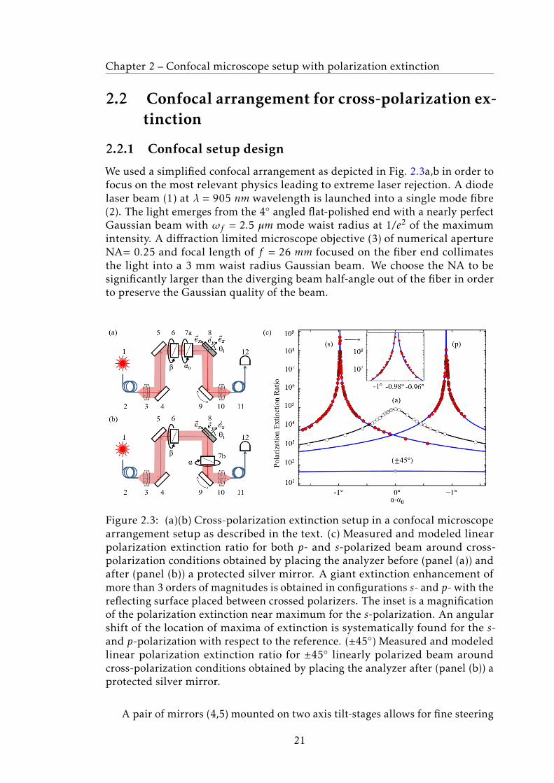
We used a simplified confocal arrangement as depicted in Fig. 2.3a,b in order tofocus on the most relevant physics leading to extreme laser rejection. A diodelaser beam (1) at λ = 905 nm wavelength is launched into a single mode fibre(2). The light emerges from the 4◦ angled flat-polished end with a nearly perfectGaussian beam with ωf = 2.5 µm mode waist radius at 1/e2 of the maximumintensity. A diffraction limited microscope objective (3) of numerical apertureNA= 0.25 and focal length of f = 26 mm focused on the fiber end collimatesthe light into a 3 mm waist radius Gaussian beam. We choose the NA to besignificantly larger than the diverging beam half-angle out of the fiber in orderto preserve the Gaussian quality of the beam.
Figure 2.3: (a)(b) Cross-polarization extinction setup in a confocal microscopearrangement setup as described in the text. (c) Measured and modeled linearpolarization extinction ratio for both p- and s-polarized beam around cross-polarization conditions obtained by placing the analyzer before (panel (a)) andafter (panel (b)) a protected silver mirror. A giant extinction enhancement ofmore than 3 orders of magnitudes is obtained in configurations s- and p- with thereflecting surface placed between crossed polarizers. The inset is a magnificationof the polarization extinction near maximum for the s-polarization. An angularshift of the location of maxima of extinction is systematically found for the s-and p-polarization with respect to the reference. (±45◦) Measured and modeledlinear polarization extinction ratio for ±45◦ linearly polarized beam aroundcross-polarization conditions obtained by placing the analyzer after (panel (b)) aprotected silver mirror.
A pair of mirrors (4,5) mounted on two axis tilt-stages allows for fine steering
21

Chapter 2 – Confocal microscope setup with polarization extinction
of the collimated beam axis. Next the beam travels to a linear polarizer (6)oriented at an angle β and mounted on a piezoelectric stepping stage rotatingwith 20 µrad resolution around the optical axis. The beam travels then towardsa mirror (8), the key element of this experiment, either by passing first throughan analyzing polarizer (Fig. 1.1a) oriented at an angle α0 for the control mea-surement (7a), or by passing through the analyzer oriented at an angle α after areflecting surface for the test experiment (7b). We mounted the analyzer also ona piezo stepper fine rotation stage. The mirror (9) mounted on two-axis piezocontrolled tilt stage steers the beam into a microscope objective (10) identicalto (3) focusing the light into the core of a single mode fiber (11) identical to (2)allowing for Gaussian TEM00 modal confocal filtering and optical detection (12)at the other end of the 5m fiber cable.
2.2.2 Confocal setup concept
This confocal arrangement simulates the essential components of the resonantfluorescence confocal microscopes. The reflecting surface plane (8) at 45◦ of inci-dence, defines the standard p and s state of polarization with projections along~ex and ~ey respectively. The reflecting test surfaces in position (8) of Fig. 2.3a,bwe used in this work were commercial protected silver, aluminum and dielectrichigh reflectivity Bragg mirrors, evaporated gold film, as well as non-polarizingbeam-splitter cubes. All such reflecting surfaces are typically used in diffractionlimited confocal microscopes. The results were qualitatively very similar for allthese reflecting surfaces. We choose to show here the data measured with silvermirrors only, this with the exception of data measured for comparison on a glasssurface reflecting from air as discussed at chapter 4.
We now discuss the measurements in the configuration shown in Fig. 2.3b, forwhich the reflecting test surface is sandwiched between the polarizer and the ana-lyzer. First, the polarizer angle β is adjusted near 0 or π/2, for p- or s-polarizationrespectively, while setting the analyzer angle α near cross-polarization at β±π/2.Then the polarizer and analyzer are subsequently finely rotated to reach maxi-mum extinction at values β and α respectively. Once the optimization reached, βremains untouched and the analyzer in its rotator is subsequently placed beforethe reflecting surface just after the polarizer for our control extinction measure-ment (Fig. 2.3 a). The analyzer angle must be then be adjusted to a new value α0in order to recover maximum nominal extinction specification inherent to thepolarizers; α0 defines then the p or s reference. The extinction data measuredas a function of the analyzer angle α in reference to α0 are shown in Fig. 2.3cfor the control measurement (Fig. 2.3a) as well as for the p- and s-polarizationsin the configuration (Fig. 2.3b). Two striking observations stands out. (i) For allthe tested reflectors indicated above, the extinction ratio obtained this way wasenhanced beyond the 108 range when the test mirror surface was sandwichedbetween the polarizer and the analyzer, reducing this way significantly the polar-ization leakage of the polarizers. (ii) The analyzer angle for maximum extinctionis shifted away from α0 by +0.898◦ and −0.977◦ for the p- and s-polarizationrespectively, a significant angular deviation given our resolution of about 10−3
22

Chapter 2 – Confocal microscope setup with polarization extinction
deg. In the chapter 3, we provide a first explanation for these two strikingobservations.
2.2.3 Confocal setup realization
Figure 2.4: Experimental realization of the cross-polarization extinction setup ina confocal arrangement (left). Coupling of the laser source is done in a separatestep (right). Red solid and dashed lines indicate the excitation and the reflectionray path respectively as explained in the text.
The exact realization of the schematic design described in section 2.2.1 isshown in Fig. 2.4. The unit on the right of Fig. 2.4 is used for coupling thelaser beam into the single mode fiber (7). The unit on the left corresponds tothe basic confocal arrangement used later in this work for polarization extinc-tion measurement and mode imaging. Alignment procedure of both units isexplained in next section 2.2.4. In what follows, we discuss and characterizeall necessary components for our experiment, like coupling unit, test surfaces(including mirrors and beam-splitter cube), detector, polarizers and rotators.
Beam steering mirrorsIn both units, we implement a beam-walk technique using a pair of protectedsilver mirrors (2,10) (Thorlabs mirrors, protected silver PF10-03-P01 - Ø1) with areflectance higher than 96% for laser wavelength 905 nm (Fig. 2.4). This processis used to ensure that the laser beam is aligned and it involves a successiveadjustment of the two steering mirrors in such a way that a maximum intensityis reached at the detector.
Test surfacesThe reflecting test surfaces in position (13) of Fig. 2.4 (left) we used in this work
23

Chapter 2 – Confocal microscope setup with polarization extinction
were commercial protected silver (Thorlabs mirror, protected silver PF10-03-P01- Ø1), aluminum (Thorlabs mirror, aluminum PFSQ20-03-G01) and dielectrichigh reflectivity Bragg mirrors (Thorlabs mirror, dielectric BB1-E03 - Ø1), evap-orated gold film (Thorlabs mirror, gold PF10-03-M03), as well as non-polarizingbeam-splitter cubes (Thorlabs non-polarizing cube beam-splitters 30:70). Allsuch reflecting surfaces are optimized for the laser wavelength 905 nm andtypically used in diffraction limited confocal microscopes.
ObjectivesIn both units, we use same objectives (Olympus Plan Achromat Objectives, NA=0.25, f = 26mm) for beam collimation or for focusing the laser light into singlemode fibers. The collimation of the light beam is optimized by means of aretroreflector (Thorlabs, TIR Retroreflector Prisms PS975-M) which we placejust after the collimator (9) and before the mirror (10). The dashed line in Fig. 2.4(right) indicates the reflection ray path. Then, the light beam is again focused bythe collimation objective (9) onto the single mode fiber (7) and is back-reflectedinto the laser coupling unit. We used a beam-splitter (3) with a transmissionratio of 70:30, a plano-convex lens (4) ( Thorlabs LA1131, f = 50 mm) and aphotodetector (5) (Thorlabs PDA36A-EC - Si Switchable Gain Detector, 350 -1100 nm) with internal gain to check the reflected light. Next, the z-position ofthe collimation objective (9) is finely adjusted until maximizing the signal onthe detector. Indeed, the focal plane of the objective coincides with z-positionfor which all rays of light are focused into the single mode fiber and thus lead-ing to a high signal value on the detector. Here, the focused spot waist radiusi.e the fiber Gaussian mode size ωf , is given by ωf = λf /πω0 = 2.5 µm with fis the focal length and ω0 = 3mm is the beam radius of the collimated laser beam.
Polarizers and rotatorsSelecting the appropriate polarizers enables excellent extinction ratio perfor-mance. For this experiment, we used the best quality commercial linear polariz-ers with an extinction in direct cross-polarization limited to 105 for nanoparticlethin film polarizer (Thorlabs LPVIS050) and to 106 for Glan-Thomson crystalpolarizers (Thorlabs GTH10M). Both polarizers are mounted on a piezoelectricstepping stage rotating (attocube systems, ANR240/RT - rotator 360° endless)with 20 µrad resolution around the optical axis. A digital controlling unit (at-tocube systems, ANC 350 multi-functional piezo controller for driving attocube’srotators) is used to drive the rotators of the polarizer and the analyzer.
DetectorIn this experiment, we used a photo-detector (Femto OE-200- Si-photodiode)which converts the incident optical signal into voltage. The resulted signal afterphoto-detection is measured on a voltmeter. The photo-detector is operatingfrom f W to mW and has an adjustable conversion gain from 103 to 1011V /Wwith a bandwidth up to 500 kHz. One of the most important measures thatquantify the sensitivity of photo-detectors is the Noise Equivalent Power (NEP),usually expressed in Watts per square root of Hertz (W/
√Hz). It corresponds
24

Chapter 2 – Confocal microscope setup with polarization extinction
to the input signal power that results in a signal-to-noise ratio (S/R) of 1 in a1 Hz output bandwidth. Basically, this represents the threshold above whicha signal can be detected. For most detectors, the output noise density can bemeasured without incident light when the optical input is completely darkened.In our case, the signal is detected using an integration time 5 ms in a bandwidth∆f = 200 Hz, with a detector of NEP down to 6f W /
√Hz. The theoretical mini-
mum detectable power using such detector is then NEP ×√∆f = 84.85 f W .
2.2.4 Confocal setup alignment
The laser coupling unit (Fig. 2.4 (right)) is made of a diode laser beam (1) (TOPAG3-5mW output power at 905 nm) of laser type 3R specified with a wavelengthof 905 nm, microscope objective (6) mounted on a z-translation stage, beamsteering mirrors (2) and a beam-splitter 70:30 (4). A photodetector (5) in com-bination with a plano-convex lens (4) ( Thorlabs LA1131, f = 50 mm) willbe used for measuring the coupling of the laser in the confocal arrangementFig. 2.4(left). Laser coupling can pose many challenges, like optical distortionsand losses. First, we start with measuring the laser power output using a powermeter sensor, the measured power before mirror (2) is about 5mW . The objective(6) is connected to a single mode fiber (7) which is placed in polarization pad-dles (8) (Thorlabs Manual fiber polarization controllers FPC560) to control therandom polarization of the light inside the fiber. Next, a beam-walk techniqueis implemented by means of mirrors (2) to ensure a maximum output intensityat the collecting fiber (7). The measured laser power at the output of the fiberpolarization controller is about P0 = 1 mW . After the laser coupling is done, thecollimating and collecting objectives of the confocal arrangement (Fig. 2.4(left))are aligned with respect to the optical axis by means of a z-translation stage.The measured laser power after collimator (9) and before mirror (10) is about70%P0 which means that the lens causes 23% loss of light at the laser wavelength905 nm. Then, a beam-walk technique is again used to ensure that the laserbeam is aligned. The laser power after all mirrors (without any polarizers) andafter focusing into the fiber (6) (Fig. 2.4(left)) is about 50%P0. This value is goodenough for performing our experiment, but it is possible to reach an outputpower of more than 0.5 mW , by using high power industrial fiber lasers to avoidcoupling losses in fiber optic.
2.2.5 Conclusion
In conclusion, we can comment that the confocal arrangement has a simplisticdesign but it requires a high degree of polarization control and alignmentprecision. In particular, the measured cross-polarization extinction was fora long time experimentally limited to 108 value. Considerable progress hasbeen made over the last year of the Ph.D. and we have reached a record level ofabout 1010 for which the limiting factor was the dark noise of our detector. Thistopic will be discussed further at the end of chapter 4. In next chapter, we will
25

Chapter 2 – Confocal microscope setup with polarization extinction
explain the physical origins of the huge cross-polarization extinction in confocalmicroscopy.
26

Chapter 3
The physical origins of cancellationof polarization leakage
Adapted from [1]:Meryem Benelajla, Elena Kammann, Bernhard Urbaszek, and Khaled Karrai,”The physical origins of extreme cross-polarization extinction in confocal mi-croscopy”, arXiv:2004.13564 (2020).
3.1 Polarization leakage equation
Intuitively, the significant reduction of the polarization leakage field must findits root in a destructive interference effect. The first challenge towards findingan answer to our problem is to offer a model of the polarization leakage. In orderto determine the light field at various planes such as after the polarizers andmirrors, we define a right hand coordinate system ~p, ~s transverse to the opticalbeam propagation axis ~p ×~s according to the definition of p- and s-polarizationwith respect to the plane of incidence with the test surface (8) of Fig. 2.3b. Forclarity, ~s ≡ ~ey is perpendicular to the incidence plane. In this section, we will testfirst the simplistic idea that the collimated laser beam can be approximated by aplane wave. We use a Jones matrices formalism projecting the field componentsalong ~p, ~s after each relevant optical element namely the matrix ¯̄P (β) of thepolarizer, ¯̄M of the reflecting test surface and ¯̄A(α) that of the analyzer. In thisformalism an ideal linear polarizer along ~p and ~s is represented by
¯̄Pp0=
[1 00 0
], ¯̄Ps0 =
[0 00 1
](3.1)
We will assume now that a real physical linear polarizer along ~p or ~s representedby ¯̄Pp = ¯̄L ¯̄Pp0
and ¯̄Ps = ¯̄L ¯̄Ps0 respectively and is characterized by a polarizer leakageJones matrix ¯̄L. Many conditions result in the light leakage such as light scatter-ing, misalignment of crossed polarizers, errors during the manufacturing process.The assumption we are making about the physical origin of the leakage is that itis due to lossless coherent scattering such as Rayleigh scattering inclusions in
27

Chapter 3 – The physical origins of cancellation of polarization leakage
the crystal. In particular, when light travels through a polarizing sheet made ofnanoparticles chains, it interacts with the medium and this causes the scatteringof light. Photons with a polarization direction along the chains are stronglyabsorbed, whereas the absorption is weak for the photons with a polarizationdirection perpendicular to these. Absorption causes the nanoparticles to vibrateand then re-emit the photons in random directions, but with same frequencyand wavelength. Rayleigh scattering is a type of coherent scattering interactionwhich causes the transmitted light to be (π/2) out of phase with the initial beamlight. In this interaction, the energy of the scattering particles is not changed.The second assumption, which we verified experimentally, is that the leakageshould be invariant upon an arbitrary angular rotation ϕ around the optical axis~p ×~s, namely ¯̄L = ¯̄R(ϕ) ¯̄L ¯̄R(−ϕ) where the rotation matrix ¯̄R(ϕ) is given by
¯̄R(ϕ) =[cosϕ −sinϕsinϕ cosϕ
](3.2)
We choose to represent the polarization leakage by a matrix
¯̄L =[a ib−ib a
](3.3)
where a2 + b2 = 1. Such a form is invariant upon rotation. For a high qualitycommercially available linear polarizer a2� b2, which is the case in our setupsince from our experiment we determine a2/b2 � (1.5 ± 0.5) × 105. This is themeasured nominal leakage seen in Fig. 2.3c. We note that the formalism can alsobe extended to circular polarizers, in which case a2 � b2 and the leakage stemsfrom the slight difference between the two terms.
We assume an incoming laser field ~Ep initially p-polarized that we rotate at an
angle β aligning it with the polarizer such ~E(β) = ¯̄R(β)~Ep. This field first traversesthe leaky polarizer also rotated at β such ¯̄P (β) = ¯̄R(β) ¯̄L ¯̄Pp0
¯̄R(−β) followed bythe mirror matrix ¯̄M and by the analyzer matrix rotated at an angle α namely¯̄A(α) = ¯̄R(α) ¯̄L ¯̄Ap0
¯̄R(−α) so the field ~E just after the analyzer writes
~E = ¯̄A(α) ¯̄M ¯̄P (β) ¯̄R(β)~Ep (3.4)
The calculation, shown in detail in Appendix A.2. The mirror Jones matrix for aplane wave writes
¯̄M =[rp 00 rs
](3.5)
Where rp,s are the complex valued Fresnel reflectivity coefficients rp = (εcosθi −√ε − sin2θi)/(εcosθi+
√ε − sin2θi) and rs = (cosθi−
√ε − sin2θi)/(cosθi+
√ε − sin2θi)
[27] where the test surface material enters through its complex-valued dielectricfunction ε = ε1+iε2 or equivalently its optical constant n2 = ε, which is tabulated
28

Chapter 3 – The physical origins of cancellation of polarization leakage
for noble mirror metals [28]. After a lengthy but straightforward calculation(Appendix A.3), we determine the light intensity just after the analyzer
I = a2 | rp cosα cosβ + rs sinα sinβ |2 +b2 | rp cosα sinβ − rs sinα cosβ |2
− 2abIm(rpr∗s )cosα sinα
(3.6)
The polarization extinction ratio is then simply given by 1/I . A practicalcheck for p(s) polarized light, namely for β = 0(π/2) and the correspondingcross-polarization α = π/2(0) leads to the expected finite polarization leakageI = b2 | rp/s |2. For a hypothetical perfect mirror, rp = 1 and rs = −1 making it inthis idealized case I = b2. Because the reflecting surface has real and imaginarycomponents for rs and rp, equation (3.6) shows that for a ”sufficiently small value”of b2 we can always find a choice of angles α,β that leads to I = 0, canceling thisway the undesired leakage. This is always true under condition of total internalreflection which is the case of a metallic mirror in the visible and infrared rangeand for a typical cube beam-splitter. A ”sufficiently small value” of depolariza-tion to obtain perfect cancellation means in the context of our work typicallyb2 < 6×10⁻³ when using a silver mirror as we will derive later in the text. Thereflecting test surface in combination with the polarizers rotation act to interferedestructively with the residual rotation invariant lossless polarization leakageinherent to even best commercial linear polarizers. Conversely, for a purelydielectric surface such a glass (i.e. BK7) reflecting from the air-side, for which rpand rs are both real, no full polarization leakage cancellation was possible.
3.2 Material and angular dependency
To get a better feel for the relevant parameters at work in canceling almostperfectly the polarization leakage we use the form rp = ρp exp(iϕp) and rs =ρs exp(iϕs). Consider high reflectivity mirrors for which ρp ≈ ρs ≈ 1. Solvingequation 3.6 for field cancellation leads to the first order in | b |� 1 to a set of twoequations cos(α + β) = b/ tan∆ and cos(α − β) = b tan∆ where ∆ = (ϕp −ϕs)/2.This way both α and β can be analytically calculated (Appendix A.4). In theparticular case of dielectrics reflecting from the air side for which ∆ = π/2 wesee already that there are no solutions. Instead we need the condition ∆ , π/2which is always verified in condition of total internal reflection. For pure sil-ver at λ = 905 nm, ϕp − ϕs = 192.52◦ implying tan∆ = −9.12 which in turnshows that for this particular case a solution I = 0 exist for polarizers withleakage levels b2 < 0.012. One more step is required to make use of these equa-tions towards interpreting our results because we did not find any easy wayto measure independently an absolute value α and β to the precision requiredfor our measurements. As explained in the previous section the value we canmeasure experimentally with the required accuracy is the shift α −α0. In thereference measurement with the analyzer placed directly after the polarizerwe assume that the cross-polarization condition α0 − β = π/2 holds. For thetest experiment, the equation cos(α − β) = b tan∆ is developed in the limit of
29
Chapter 3 – The physical origins of cancellation of polarization leakage
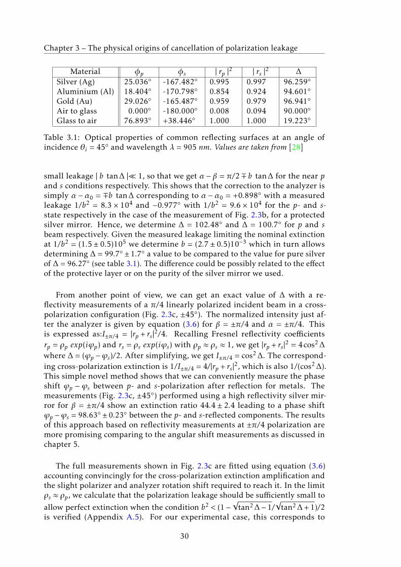
Material φp φs | rp |2 | rs |2 ∆
Silver (Ag) 25.036◦ -167.482◦ 0.995 0.997 96.259◦
Aluminium (Al) 18.404◦ -170.798◦ 0.854 0.924 94.601◦
Gold (Au) 29.026◦ -165.487◦ 0.959 0.979 96.941◦
Air to glass 0.000◦ -180.000◦ 0.008 0.094 90.000◦
Glass to air 76.893◦ +38.446◦ 1.000 1.000 19.223◦
Table 3.1: Optical properties of common reflecting surfaces at an angle ofincidence θi = 45◦ and wavelength λ = 905 nm. Values are taken from [28]
small leakage | b tan∆ |� 1, so that we get α − β = π/2∓ b tan∆ for the near pand s conditions respectively. This shows that the correction to the analyzer issimply α − α0 = ∓b tan∆ corresponding to α − α0 = +0.898◦ with a measuredleakage 1/b2 = 8.3 × 10⁴ and −0.977◦ with 1/b2 = 9.6 × 10⁴ for the p- and s-state respectively in the case of the measurement of Fig. 2.3b, for a protectedsilver mirror. Hence, we determine ∆ = 102.48◦ and ∆ = 100.7◦ for p and sbeam respectively. Given the measured leakage limiting the nominal extinctionat 1/b2 = (1.5 ± 0.5)105 we determine b = (2.7 ± 0.5)10−3 which in turn allowsdetermining ∆ = 99.7◦ ± 1.7◦ a value to be compared to the value for pure silverof ∆ = 96.27◦ (see table 3.1). The difference could be possibly related to the effectof the protective layer or on the purity of the silver mirror we used.
From another point of view, we can get an exact value of ∆ with a re-flectivity measurements of a π/4 linearly polarized incident beam in a cross-polarization configuration (Fig. 2.3c, ±45◦). The normalized intensity just af-ter the analyzer is given by equation (3.6) for β = ±π/4 and α = ±π/4. Thisis expressed as:I±π/4 = |rp + rs|2/4. Recalling Fresnel reflectivity coefficientsrp = ρp exp(iϕp) and rs = ρs exp(iϕs) with ρp ≈ ρs ≈ 1, we get |rp + rs|2 = 4cos2∆
where ∆ = (ϕp −ϕs)/2. After simplifying, we get I±π/4 = cos2∆. The correspond-ing cross-polarization extinction is 1/I±π/4 = 4/ |rp + rs|2, which is also 1/(cos2∆).This simple novel method shows that we can conveniently measure the phaseshift ϕp − ϕs between p- and s-polarization after reflection for metals. Themeasurements (Fig. 2.3c, ±45◦) performed using a high reflectivity silver mir-ror for β = ±π/4 show an extinction ratio 44.4 ± 2.4 leading to a phase shiftϕp −ϕs = 98.63◦ ± 0.23◦ between the p- and s-reflected components. The resultsof this approach based on reflectivity measurements at ±π/4 polarization aremore promising comparing to the angular shift measurements as discussed inchapter 5.
The full measurements shown in Fig. 2.3c are fitted using equation (3.6)accounting convincingly for the cross-polarization extinction amplification andthe slight polarizer and analyzer rotation shift required to reach it. In the limitρs ≈ ρp, we calculate that the polarization leakage should be sufficiently small to
allow perfect extinction when the condition b2 < (1−√
tan2∆− 1/√
tan2∆+ 1)/2is verified (Appendix A.5). For our experimental case, this corresponds to
30

Chapter 3 – The physical origins of cancellation of polarization leakage
b2 < 1.26 10−2 and for a pure silver to b2 < 6.00 10−3. Such values are infact relatively large and thus allow realistically achieving polarization leakagecancellation for most standard commercial polarizers.
3.3 Wavelength dependency
A last practical aspect to address is the wavelength dependency of this effect.For a highly reflecting mirror, the wavelength dependency is to be found inthe phase difference ∆(λ). As a result, the correction to the analyzer angleα(λ) − α0 = ∓b tan∆(λ) calculated for reaching maximum extinction is also afunction of wavelength. Hence, we see that the polarizer angle α of maximum ex-tinction shifts as a function of wavelength as ∂α/∂λ = ∓b(∂∆/∂λ)/ cos2∆ whichcan easily be evaluated using the formula of Fresnel coefficient and the cor-responding dielectric constant of the mirror relevant material. For a perfectsilver mirror and a polarization leakage of 105 we evaluate a chromaticity rateof ∂α/∂λ = 0.0019◦/nm for a wavelength around λ = 905 nm. In this particularexample, keeping the analyzer angle at value of maximum extinction for 905 nm,the wavelength could be shift by up to ±10 nm and still keep the extinction upto a level > 107.
3.4 Conclusion
At this point we could conclude our work here as we were able to explain con-vincingly all the features of the enhanced polarization extinction. Our analysishas however occulted so far a crucial point, namely the experimental fact thatthe leakage cancellation was only measurable in a confocal arrangement, a pointthat is elucidated in the next chapters. More specifically, the analysis we con-ducted leading to the main result in equation (3.6) so far was done purely for aplane wave for which the Jones matrix formalism is valid. In reality however,the finite size of the collimated Gaussian laser beam imposes a finite angularwave distribution around the angle of incidence on the mirror [29]. The Fresnelcoefficient rp and rs becomes then a function of the angular distribution [29].This as we will see, leads to significant geometrical depolarization effects in formof new optical modes limiting the total extinction to the 104 range. We will seethat a confocal arrangement filters away the depolarization modes and that theresult of this chapter turns out to be fortuitously usable.
31


Chapter 4
Modal transformation of a reflectedpolarized Gaussian beam
Adapted from [1]:Meryem Benelajla, Elena Kammann, Bernhard Urbaszek, and Khaled Karrai,”The physical origins of extreme cross-polarization extinction in confocal mi-croscopy”, arXiv:2004.13564 (2020).
4.1 Experimental modal analysis of beam reflectiv-ity
4.1.1 Experimental details
To find the origin of the unexpectedly high polarization rejection ratio > 108, weperformed an x,y scanning imaging of the detected intensity in cross-polarizationconditions. Imaging can be achieved by scanning a mirror (9) or scanning thespatial position of the collecting fiber in the focal plane of the focusing objective(Fig. 2.3b). Scanning the fiber position with respect to the fix objective has theadvantage that the optical system is fixed in space and avoids the problem ofmisalignment but mirror scanning can be faster and offer wider range of scan.In this work, we use the fiber scanning technique. The output fiber is mountedon a piezo electric scanner (Thorlabs scanner, PE4 piezo electric actuator) whichhas a maximum travel range of 15µmwhen 150 V is applied to the piezo actuatorx or y (Fig. 4.1). We use the attocube ASC500 scan and imaging controller withxy-scan generator to create the voltage necessary for the scan. Such controllerhas a maximum allowed voltage output ±15V and for this reason, we use the at-tocube scan voltage amplifier ANC200 to amplify the maximum allowed voltageby a factor 10 in order to reach the 150V at the piezo scanner. In this configura-tion, the x,y output scanners of the ASC500 are connected into the x,y DC inof the ANC200. Then, the x,y output of the ANC200 are connected to the x,ypiezo scanner. The photo-detector measured power intensity Ix,y correspondingto each pixel location x,y on the scan is collected via a single mode fibre in
33

Chapter 4 – Modal transformation of a reflected polarized Gaussian beam
combination with the femto variable gain photo-receiver (see specifications insection 2.2.3). The electrical output signal is then connected to the signal inputof the ASC500 controller. The recorded signal is imaged into a two dimensionalcolor plot using the ASC500 software.
Figure 4.1: (Left) xyz-piezo electric scanner when no voltage is applied tothe actuators. (Right) Plane at objective focus, looking into the objective backaperture towards the optical fiber entrance. x (y respectively) increasing in thedirection of the axis x (y respectively) on the drawing for voltages increasingfrom 0 to up. Manual Resolution:1µm. Piezo travel range: 15µm. Piezo drivingvoltage 150V . Piezo capacitance: 1.4µF.
4.1.2 Confocal imaging of Imbert-Fedorov modes
In the absence of a reflecting surface between the analyzer and polarizer in cross-polarization, namely the reference configuration in Fig. 2.3a, the measurementsin Fig. 4.2a,b (upper row) show a pure TEM00 Gaussian mode field attenuatedby 8.3× 10⁴ and 9.6× 10⁴ for p- and s- polarized beam, respectively. This levelis expected for the polarizer leakage specifications. In contrast, when we placethe analyzer after the reflecting test surface, the measurements show that themode splits into two lobes distributed along ~ey and located above and belowthe reflectivity plane. In this cross-polarized configuration, we find an intensity“hole” at the location of the optical fiber center. There the intensity extinction isslightly higher than 108, a factor 100 away from our actual setup sensing-limitdiscussed later in this work.
To get a feel for the measured modal transformation for p- and s-, we mea-sured and showed in Fig. 4.3 and Fig. 4.4 the evolution of the confocal lightintensity maps for different analyzer rotation angles variation δα around thesymmetrically split mode. Fig. 4.3d and 4.4d show quantitatively for p- ands-polarizations the measured positions of beam-peak shifts along ~ey and split-ting above and below the plane of incidence as a function of δα. We observeda very similar behavior for beam-splitter cubes typically used in the resonantfluorescence setup such as in reference [8, 9, 16, 18], with the difference how-ever that equivalent figure looks instead mirrored with respect to the axis ∆y = 0.
34

Chapter 4 – Modal transformation of a reflected polarized Gaussian beam
Figure 4.2: Confocal mapping of s- (a) and p- (b) laser beam in co- and cross-polarization using a scanning mirror (9). The upper and lower rows of the figuresare measurements with the analyzer placed before ( Fig. 2.3a) and after ( Fig. 2.3b)the test reflecting surface respectively, in s-polarization and p-polarization (panela and b). We plot the extinction ratio map by dividing, pixel per pixel, the co-with the cross-polarized data. In cross-polarization, a modal splitting along~ey above and below the plane of incidence is observed both for the s- and p-polarization. The dotted line circle is the 1/e intensity level of the Gaussiandistribution resulting from the confocal convolution between the focused spotand the collecting fiber mode. The location of the maxima of the modal splittinglie exactly on that circle. The diameter of this circle gives also the non-convolutedfocal spot waist diameter at 1/e2 focused on the collecting fiber end. The verticalwhite bar represents 5µm.
35

Chapter 4 – Modal transformation of a reflected polarized Gaussian beam
In all cases, such split-lobes intensity distribution is very reminiscent of aTEM01 Hermite-Gaussian mode.Figure 4.3c and 4.4c show on careful inspection that the minima of intensityor maxima of extinction do not occur exactly at y = 0 but instead are veryslightly displaced symmetrically along y for both the p- and s-polarization. Thismean that there is not a single position of the fibre location y that can lead to amaximum extinction for both p- and s-polarization at the same time. This is alsoclearly seen in Fig. 2.3c for which the extinction is beyond the 109 range for thes-polarization and 108 for p- in that particular measurement. This observationsuggest clearly that the novel modes along y do seem to assist in boosting theextinction well beyond the 108 level. We have reached a record level of 1010 forwhich the limiting factor was the dark noise of our detector. The challenge insuch experiment is to have a polarization rotator that enable stepping with smallenough rotation angles. At this point we need to find out why (i) the confocalarrangement enables the dramatic extinction enhancement as seen in Fig. 2.3c,and (ii) why does the beam shift and split at cross-polarization in Fig. 4.2 (lowerrow) and this always above and below the plane of incidence. To answer thesequestions we need to first model the spatial field distribution at the focal plane ofthe focusing lens just before the collecting single mode optical fiber (see section4.2.1) and then use the collecting fiber as the confocal Gaussian filter functionporting the light to the detector (see section 4.2.2).
Figure 4.3: p-polarized beam reflected off a silver mirror. Measured (a) and sim-ulated (b) evolution of the modal confocal imaging mapping through maximumextinction (c) for different analyzer angles δα as explained in text. In (d), thebeam peak-shift and splitting positions are shown in units of beam waist ωfat focus which we modeled for our silver mirror ∆ = 102.48◦and a leakage of1/b2 = 8.3× 10⁴
36

Chapter 4 – Modal transformation of a reflected polarized Gaussian beam
Figure 4.4: s-polarized beam reflected off a silver mirror. Measured (a) andsimulated (b) evolution of the modal confocal imaging mapping through maxi-mum extinction (c) for different analyzer angles δα as explained in text. In (d),the beam peak-shift and splitting positions are shown in units of beam waistωf at focus which we modeled for a silver mirror ∆ = 100.7◦and a leakage of1/b2 = 9.6× 10⁴
4.2 Theoretical modal analysis of beam reflectivity
4.2.1 Mirror transfer matrix in angular domain
In this section, we will model the spatial field distribution ~Ef x,y at the focal planeof the focusing lens just before the collecting single mode optical fiber. The finitesize beam before the mirror results from a Gaussian-weighted superposition ofplane waves propagating along an angular distribution ~k/k0 = u~p+ v~s+w~k0/k0
very narrowly centered around ~k0 the wave vector along the optical axis withk0 = 2π/λ as depicted in figure 4.5. In the paraxial approximation u and v areboth � 1, so they represent the angular spread of the collimated beam. Thefocusing lens transforms each plane wave field ~Eu,v of the angular distributioninto a field density ~Ef x,y in the focal plane, hence the beam reaching the focalplane at distance f result from a coherent superposition of all such focusedcomponents (Appendix B.2). Assuming that all these waves are paraxial andapplying the Fresnel approximation [30] one can establish that
~Ef x,y =−iλf
exp(
+ ik0f) +∞"−∞
~Eu,v exp[
+ ik0(xu + yv)]dudv (4.1)
The integrals run normally within the maximum boundaries -1 and 1 for u,v, but for mathematical convenience they are extended to infinities as thisdoes not affect the result in a paraxial approximation, namely because ~Eu,vvanishes rapidly when u, v are no longer much less than unity. In what follows
37

Chapter 4 – Modal transformation of a reflected polarized Gaussian beam
Figure 4.5: Geometry of beam reflection off a mirror. The incident beam hasa Gaussian field distribution in the transverse plane. The transverse u, v andlongitudinal w wavenumbers depend on the angle of incidence as explained intext.
we will drop the propagation phase term exp+ik0f as we from now on justconcern with establishing the field at focal plane only. The next step is to obtainthe angular distribution ~Eu,v. Such problem was modeled for a Gaussian fielddistribution in [31] by Aiello and Woerdman. We derive here a simplified versionconveniently describing the essential physics needed to model our observations.We begin with the field just before the polarizer for which we assume a linearlypolarized Gaussian-field normalized angular distribution ~E0uv
~E0uv =E0
πθ20
exp(− u
2 + v2
θ20
)[cosβsinβ
](4.2)
The mode divergence θ0 = 2/(k0ω0) = ω0/l results from the finite size of thecollimated laser beam with beam radius ω0 ≡ 3mm, and the Rayleigh rangel = k0ω
20/2 is 104 m, a value much larger than the size of our experimental setup
allowing us to ignore the role of beam propagation up to the focusing lens. Withthis convention a p(s) polarized light is obtained at β = 0(π/2).When the beam reflects off the test surface, each plane wave component acquiresan angle dependent Fresnel reflection coefficient rp,uv and rs,uv that are functionnot only of θi but also of u, v [29]. Consequently, for each plane wave component,we choose a coordinate system ~ep, ~es, ~k/k0 that defines a local incidence plane
for that wave. The longitudinal basis vector is ~k/k0 and the transverse ones are~es =~k/k0 ×~ez and ~ep = (~k/k0 ×~ez)× (~k/k0) in the s- and p- planes respectively. Toobtain the reflectivity of the mirror for each plane wave, we determine firstthe weights of p- and s- field components, given by the weighted projectionsrp,uv(~ep · ~E0uv) and rs,uv(~es · ~E0uv). We determine then the resulting reflected field
transverse field along the corresponding reflected basis ~es,R = ~kR/k0 × ~ez and~ep,R = (~kR/k0 ×~ez)× (~kR/k0) such ~Euv = rp,uv(~ep · ~E0uv)~ep,R + rs,uv(~es · ~E0uv)~es,R. Here~kR is the mirrored wave vector after reflection. In the paraxial limit, for a beamimpinging, the Fresnel coefficients are developed to the first order in u aroundθi and v around 0, giving rp,uv = rp + u ∂rp/∂θi and rs,uv = rs + u ∂rs/∂θi . The
38

Chapter 4 – Modal transformation of a reflected polarized Gaussian beam
first order derivatives ∂rp/s uv/∂v in the s-plane vanish both for rp and rs leavingjust derivative r
′p = ∂rp/∂θi and r
′s = ∂rs/∂θi . We calculate the components of
the incoming and reflected basis vectors ~ep, ~es, ~k/k0 and ~ep,R, ~es,R, ~kR/k0 in theparaxial limit u,v << θi . After a lenghty but straightforward calculation weobtain the reflected field distribution after the mirror for each angle u,v (seeAppendix B.1) . We express the result conveniently in terms of Matrix notation~Euv = ¯̄Mu,v
~E0uv where
¯̄Mu,v =[rp 00 rs
]+u
[r ′p 00 r ′s
]+ v
rp + rstanθi
[0 −11 0
](4.3)
Upon inspection of the expression 4.3 for symmetries we see now that the re-flectivity Jones matrix transforms an impinging perfect Gaussian mode, suchas equation (4.2), into the sum of TEM00, TEM01 and TEM10 Hermite-Gaussmodes. The indices for TEMnm indicate the number of nodes along the ~p and~s direction repectively. The first term in the right hand side is the normal testsurface reflectivity we used in the first part of this paper. The second term isresponsible for generating a TEM10 mode along ~p in the plane of incidence. Thisterm is in fact responsible for the Goos-Hänchen effect [32–37], as it has itsphysical origin in the angular dispersion of the reflectivity terms at θi . Here thedifferent plane wave components acquire slightly different phases upon reflectiv-ity shifting the beam in the plane of incidence. Because this matrix is diagonal,we see that for a perfect p- or s-polarization the Goos-Hänchen effect does notcontribute to depolarization. The third term, the most relevant to this work, isresponsible for generating an out of plane of incidence TEM01 mode with twolobes along ~ey . This term is the physics responsible for the Imbert-Fedorov ef-fect [19,20,22,33–38] known to deviate a reflected light beam above or below theplane of incidence depending on its right handed or left handed polarization he-licity. The calculation detailed above shows that this term originates purely fromgeometrical projections in which the gradual phase-shift gained by each planewave component upon reflection, sums to a cross-diagonal matrix that mixesthe p- and s- phase shifted reflected plane wave components. Consequently thisterm is responsible for an intrinsic reflectivity induced depolarization for p- ands-polarization even when using ideally perfect polarizers. Because of the purelygeometrical projections nature of the argumentation, compelling connectionsbetween the Imbert-Fedorov effect, Berry’s phase and spin-Hall effect of lightare discussed in the literature [22, 38]. Because of the direct proportional depen-dency of this matrix on the angle v and in particular its sign, it creates a TEM10mode asymmetric along ~ey , adding/suppressing field to/from the symmetricmain mode displacing this way its weight above or below the plane of incidencedepending on its helicity. This can be easily verified using a circular polarizationversion of equation (4.2) with the Jones matrix equation (4.3). From this simplederivation, it is worth appreciating that in the paraxial approximation equation(4.3) express both Goos-Hänchen and Imbert-Fedorov effects in an elegant andcompact way. At this point, we can see from a symmetry argument that our con-focal arrangement enhances cross-polarization extinction. Without the confocalarrangement, the extinction would have been naturally limited in the 104 range
39

Chapter 4 – Modal transformation of a reflected polarized Gaussian beam
in our experiment as we will discuss in the section 4.2.3.
4.2.2 Mirror transfer matrix in space domain
In the following step we express the field distribution transmitted through thepolarizer, the mirror and analyzer at the back aperture of the focusing lens~Euv = ¯̄A(α) ¯̄Mu,v
¯̄P (β)~E0uv used in the Fourier transform equation (4.1). Beforeproviding the general solution, we get first a feel for the physical parametersgoverning the Imbert-Fedorov cross-polarized mode. For this, we consider thespecial case of a p- or s-polarized light impinging on the mirror and subsequentlyanalyzed in cross-polarization configuration. Here, only the third matrix onthe r.h.s of equation (4.3) is relevant, all other terms cancel. After some algebra(Appendix B.2) we obtain the cross-polarized field for the p(s) incident light
~Ef ⊥ =±E0
πω2f
rp + rstanθi
y
lfexp
(−x2 + y2
ω2f
)~es (4.4)
here the focused spot waist radius ωf = λf /πω0 ' 2.5µm is the fiber Gaussianmode size and lf = k0ω
2f /2 corresponding Rayleigh range, in our case 21.7µm.
We notice that the field is an antisymmetric function of y with two lobes with op-posite phase located at y = ±ωf /
√2 above and below the plane of incidence. The
field peak intensity normalized to the maximum of co-polarized peak intensityis proportional to the ratio ωf /lf which is nothing else than θf = 2/(k0ωf ) thehalf cone angle of the focused beam which in our experiment is the numericalaperture of the single mode fiber. An important result emerges, namely that thelens amplifies dramatically the Imbert-Fedorov mode field strength. It is easy toshow that the amplification factor of the light intensity is ω2
0/ω2f when compar-
ing the peak strength just after the reflecting test surface (i.e ω0 = 3mm) and atthe focal plane. In our case we obtain an amplification of 3mm/2.5µm = 1200.This is the reason for which we can detect this mode so clearly in a confocalconfiguration.
The other essential physical parameter that governs the Imbert-Fedorovmode field intensity is the sum rp + rs given by the material reflecting properties.To get a more physical insight we use the representation rp = ρp exp(iϕp) andrs = ρs exp(iϕs) that can be conveniently symmetrized using ρs = ρ+ δρ/2, ρp =ρ − δρ/2 for the reflectivity and ∆ = (ϕp −ϕs)/2 the phase difference. This waywe obtain
rp + rs = 2ρcos∆+ iδρ sin∆ (4.5)
to within a constant proportional phase term expi(ϕp +ϕs)/2 identical for allmodes of equation (4.3). We now see that the difference ϕp −ϕs governs theintensity and the phase of the Imbert-Fedorov mode. For instance in the caseof the air side reflectivity off a perfect dielectric we have ϕp − ϕs = π, hencerp + rs = iδρ, so the Imbert-Fedorov mode field intensity is directly proportional
40

Chapter 4 – Modal transformation of a reflected polarized Gaussian beam
to the pure differential reflectivity between the p and s waves. In contrast, fordielectrics under total internal reflectivity and for metals we have δρ ≈ 0 andρ ≈ 1 so that rp + rs = 2cos∆. In this case the strength of the depolarizing modeis fully governed by the phase difference ϕp −ϕs. We conclude that mappingthe Imbert-Fedorov mode fields in a confocal microcopy setup provides a directand sensitive access to the differential reflectivity amplitude and phases of areflecting surface. To move forward with our analysis on the more generalcase we have performed the Fourier optics transformation equation (4.3). Thecalculation, shown in detail in Appendix B.3. The result is that the field image atfocal plane for the test experiment with the mirror placed between the polarizersis ~Ef xy = ¯̄A(α) ¯̄Mx,y
¯̄P (β)~E0x,y where the effective reflectivity Jones matrix is givenby
¯̄Mx,y =[rp 00 rs
]+ i
xlf
[r ′p 00 r ′s
]+ i
y
lf
rp + rstanθi
[0 −11 0
](4.6)
The spatial distribution of the field ~E0x,y results from the lens transforming theunperturbed linearly polarized laser field angular distribution of equation (4.2)into a spatial normalized distribution now at the focal point such
~E0x,y =−iE0
πω2f
exp(−x2 + y2
ω2f
)[cosβsinβ
](4.7)
This result turns out to be within a Gouy phase −i at focus, the one discoveredin a different context in the insightful and pioneering work of Aiello et al. [39].In their work the authors provided within a paraxial approximation, a completeanalytical solution for the field distribution of a single mode Gaussian beamreflected off a mirror. The essential finding from our work is that the confocalarrangement transforms the collimated beam waist ω0 and Rayleigh length land of Aiello et al. [39] field distribution at the mirror plane, into lf and ωf inour case. This result appears benign at first but as discussed earlier amounts to asizeable amplification of the weak mode intensity in proportion to ω2
0/ω2f . Aiello
et al. [39] showed that it is the finite size of the beam at the reflecting surface thatare responsible for the additional field terms that affect the initial Gaussian mode.From our work it is becoming now clear here that using a confocal arrangement,the size of the beam at the mirror is not relevant to our measurements butrather the size of the focused beam that plays a crucial role. This fact, at firstnon-intuitive, provides a valuable advantage to explore experimentally the cross-polarization geometry with sufficient sensitivity and a very fine spatial resolution.In particular, high extinction cross-polarization extinction is kin to the “weakmeasurement procedure” of Aharonov et al. [40, 41] which we extend here to aconfocal arrangement enabling the added benefit of spatial resolution. Recentliterature [22] provides an interpretation for the depolarization as resultingfrom an effective spin-orbit interaction of light occurring at the mirror surfacemanifesting itself in the form of a spin-Hall effect of light [42]. In the work,we restrict ourselves to a purely modal interpretation and leave the discussionconcerning spin-orbit aside.
41

Chapter 4 – Modal transformation of a reflected polarized Gaussian beam
4.2.3 Effect of confocal filtering
The one final point we need to address to get a full quantitative interpretationof our experiment is to address the effect of the confocal filter function of thecollecting fibre. The single mode fiber collects and ports the field to the photo-detector, it does this however by acting as a Gaussian spatial filter. For oursymmetric setup shown in Fig. 2.3 we illuminate and collect light with a singlemode fibers of identical mode size, and with identical collimating and focusinglenses. The spatial filtering is a convolution between the field spatial distributionat focal plane and the fiber Gaussian mode amounting to a detected field strength~ED location x0, y0 with respect to the optical axis. The results of the calculationfor the field are the following (Appendix C.1). First we get the mapping of thereference field without use of polarizer and reflecting surface as seen by thedetector
~ED0,0 = − iE0
2exp
(−x2
0 + y20
2ω2f
)[cosβsinβ
](4.8)
We note that beam waist at focus appears now to be broadened by a factor√
2when comparing with the distribution of equation (4.7). Second we found thatthe confocal filtering by convolution with a Gaussian mode leads to a modifiedeffective Jones matrix for the reflecting surface acting on the field as seen fromthe detector (see Appendix C.2)
¯̄MDx0,y0=
[rp 00 rs
]+ i
x0
2lf
[r ′p 00 r ′s
]+ i
y0
2lf
rp + rstanθi
[0 −11 0
](4.9)
With the confocal filtering, the Goos-Hänchen and the Imbert-Fedorov fieldsterms (i.e. the second and third terms of the r.h.s in the equation) are halvedwhen compared to equation (4.6). The Jones matrix related to the polarizersand polarization leakage remain unchanged. With this last correction, we havenow all the equations required in order to simulate the modal transformationinduced by a reflecting surface acting on a polarized Gaussian beam and thisfor any arbitrary polarization and polarization leakage level. Finally the fullscanning confocal mapping of the detected field is given by the analytical form
~ED(x0, y0) = ¯̄A(α) ¯̄MDx0,y0¯̄P (β)~ED0,0 (4.10)
The first important result we are getting from equation (4.10) and the mirrormatrix term in equation (4.9) is when the location of the fiber center and the focalspot axis coincide, namely for x0 = 0 and y0 = 0. In this case the result is the sameas found in the simplified plane wave analysis of chapter 3 and the equation ofpolarization cancellation given in equation (3.6) holds fortuitously. This is thecase because the filtering function of the confocal arrangement eliminates thehigher depolarizing modes. Without the confocal filtering (see Appendix D), thenormalized integrated total intensity in cross-polarization detected in wide fieldimaging of the focused point, or for collected with a wide core multimode fiber,
42

Chapter 4 – Modal transformation of a reflected polarized Gaussian beam
is obtained using equations (4.4) and (4.7):!| ~Ef ⊥ |2 dxdy!| ~E0x,y |2 dxdy
=14
| rp + rs |2
tan2θi
(ωflf
)2(4.11)
For our experimental parameters and using equation (4.5), the collected depo-larized field would limit the extinction to 1.56 × 10³ and 2.1 × 10³ for p- ands-polarized beam respectively. This demonstrates the key role of the confocalarrangement for the giant polarization extinction reached in the state of the artresonance fluorescence measurements [8, 9, 16, 18].
The second significant result is illustrated, applying equation (4.10) on apurely p- or s-polarized beam measured in cross-polarization, by mapping thefocused spot position (x0, y0) across the single mode fiber end. The result isan intensity map displaying two lobes maxima located at the fiber location atx0max = 0 and y0max = ±ωf above and below the plane of incidence. This is incomplete agreement with our measurements as seen in Fig. 4.2 for silver. Weconfirmed quantitatively these findings for Bragg mirrors and thin-film basedbeam-splitter cubes. As seen in figure Fig. 4.3 and Fig. 4.4, equation (4.10)maps closely the evolution of the mode transformation near cross-polarizationcondition for a metallic surface. In our experiment the material parameter of thehigh reflectivity surface that governs most of the effects we observed is the phasedifference ϕp −ϕs. In particular for high reflectivity materials the intensity ofthe lobe maxima at cross-polarization are obtained from equation (4.10) at fiberlocation (x0, y0) = (0,±ωf )
| ~ED(0,±ωf )/ ~ED0,0 |2=14e
| rp + rs |2
tan2θi
(ωflf
)2(4.12)
See Appendix C.3 for more details. In particular for high reflectivity mate-rials, from equation (4.5) we have | rp + rs |2= 4cos2∆. For a pure silver surface∆ = 192.52◦, the lobe intensity should be 5.9 × 10⁻⁵. For our independentlymeasured values of ∆ = 102.48◦ and ∆ = 100.7◦, we should be finding 2.35×10⁻⁴
and 1.74× 10⁻⁴ for p- and s- polarization respectively. We measure typical lobemaxima in the range of 0.3 to 1.4×10⁻⁶. For a reason not yet elucidated, our max-imum measured intensities are weaker than modeled. We believe that we are stillmissing a full quantitative understanding in the way the receiving fiber filtersnon Gaussian modes. Indeed the sensitivity of our setup should have permittedto detect the higher terms modes TEM11 that have a symmetry xy. Such modesoriginate from the finite sized waist of the Gaussian beam making it naturallydivergent [43]. In fact, we can use the exact formalism developed above to showthat such terms originate also from geometrical projections around the opticalaxis. This time the projection is not involving any reflecting surface but just thenatural divergence of the beam before the lens, leading to a gradual phase-shiftgained by each plane wave component here again depolarizing naturally thebeam. Applying the Fourier transform due to the focusing lens and keeping in
43

Chapter 4 – Modal transformation of a reflected polarized Gaussian beam
mind the convolution imposed by the collecting fiber, we calculated that theexpected clover shaped mode is peaking at the four location (x0;y0) = (±ωf ;±ωf )with an intensity given by (see Appendix E):
| ~ED(±ωf ,±ωf )/ ~ED0,0 |2=1
4e2
( ωf2 lf
)4(4.13)
A result corroborated in ref [43]. Using this expression for our experimentparameters, the mode peak intensity should be 3.8×10⁻⁷ a value that is wellwithin our sensitivity range. It is a puzzling fact that we did not observe anytrace of this TEM11 signal. There is no doubt however that this mode is presentas measured in [43] , this is why we believe that our understanding of the waythe optical fiber is filtering the signal is not complete yet.
4.2.4 Understanding effect of metal mirrors reflectivity
To get a first impression of what a metallic mirror does to a Gaussian beam, itis instructive to use the small angle approximation for the reflectivity matrix(equation (4.9)). The result is expressed as a function of the physical param-eters related to the mirror material, the angle of incidence and the Gaussianbeam Rayleigh length. The general reflectivity coefficients are given for reflect-ing material of complex dielectric function ε̃ under incidence angle θi by thefollowing [27]:
rp =ε̃cosθi −
√ε̃ − sin2θi
ε̃cosθi +√ε̃ − sin2θi
(4.14)
and
rs =cosθi −
√ε̃ − sin2θi
cosθi +√ε̃ − sin2θi
(4.15)
In the following we concentrate on the case of total internal reflectivity (i.e.metallic mirrors). We approximate in what follows ε̃ � −ε with ε is a real andpositive number� 1. Using this definition (see Appendix F), we can write theFresnel reflectivity coefficients in the limit of small angle approximation as:
rp � 1− 2ε
+2i√ε
+ iθ2i√ε
(4.16)
and
rs � −1 +2ε− 2i√ε
+ iθ2i√ε
(4.17)
Inserting equation (4.16) and (4.17) into equation (4.9), we find that the Jonesmatrix for a reflecting surface in the limit of small angle approximation is given
44

Chapter 4 – Modal transformation of a reflected polarized Gaussian beam
by:
limθi→0
¯̄MDx0,y0=
(1− 2
ε+
2i√ε
)[1 00 −1
]+ iθ2i√ε
[1 00 1
]− θi√
ε
x0
lf
[1 00 1
]− θi√
ε
y0
lf
[0 −11 0
](4.18)
The same formula is also conveniently expressed as a function of the beam waistradius and photon wavelength
limθi→0
¯̄MDx0,y0=
(1− 2
ε+
2i√ε
)[1 00 −1
]+iθ2i√ε
[1 00 1
]− θi√
ε
λx0
ω2f
[1 00 1
]− θi√
ε
λy0
ω2f
[0 −11 0
](4.19)
This formulation is useful to get a feel for how the physical parameters governthe various component in the modal transformation of Gaussian beam reflectedoff a mirror. The first limit is to understand that in the case of an ideally perfectmirror in which case (ε̃ = −ε)→−∞, the mirror reflectivity is
lim(ε̃=−ε)→−∞
¯̄MDx0,y0=
[1 00 −1
](4.20)
With this matrix, the reflected mode remains Gaussian and its polarization ismirrored but remain "pure". For finite values of ε, new terms appear that nowinvolve the mirror material properties, the angle of incidence θi , the Gaussianbeam waist and wavelength (or Rayleigh length lf ). The first matrix providesreflectivity at vanishing angle of incidence. It shows first that the p and s reflec-tivity are 180◦ out of phase. It is interesting to note that for a purely real andnegative dielectric constant ε̃ = −ε the matrix pre-factor contains an imaginaryterm. This is the case of total internal reflectivity. This term delays or advanceof the reflected light for the p or s polarization with respect to the incidentlaser field, the relative phase between p and s is constant at 180◦. The secondterm leads to a phase retardation that becomes increasingly different for p ands at finite non-vanishing angle θi , the phase difference scales as θ2
i . This is theterm that introduces ellipticity on a linearly polarized field tilted with respectto the incident plane and enables a perfect compensation of the polarizationleakage in our experiment. While the first two matrices describes the reflectivityof a plane wave off a metallic mirror, the third and fourth matrix relate to thefinite size of a light beam. They do vanish in the limit of infinite beam waistsize, namely strictly speaking in the case of a plane wave. These two matricestransform the initial Gaussian mode into the next higher symmetry modes witha node at the location of the fiber position origin. The intensity of these modesscale like inverse Rayleigh length, which represent the depth of field of thelight focused onto the confocal filter aperture. The stronger the focusing thelarger the weight of the higher order modes. We learn here that in a confocalarrangement, the size of the beam at the mirror location is not directly relevant;instead, the size of focused beam at the location of the collecting aperture drivesthe intensity and the size of the new modes. This remark, helps determining newmeasurement strategies compared to previous works. In particular in earlierpublications [42] [39], the Gaussian beam was focused on the reflecting surface.
45

Chapter 4 – Modal transformation of a reflected polarized Gaussian beam
This is no longer a limitation allowing to work with collimated beams over largedistances and illuminating larger portions of mirror materials.
The third matrix is responsible for the Goos-Hänchen effect [32–37]. Onclose inspection, one can see that matrix distributes continuously along x (i.e. inproportion to x0 ) the weight to the reflectance components in the plane of inci-dence across the Gaussian beam field changing its sign past the node at origin.This field added to the original Gaussian distribution results in a displacementof the maximum of the beam intensity in the p-plane. The effect is understoodas beam displacement in the plane of incidence. The displacement is positive,namely along +~p for an s- polarized Gaussian beam and is negative (along -~p)for a p-polarized beam. Measurements for metals were published in [44]. Thephysics behind this effect is the finite penetration depth of the optical beamunder the surface of the mirror. The penetration depth depends on the angleof incidence. The larger the angle the shorter the penetration depth. The finitesize of the beam is formed by a superposition of plane waves with a distributionof angle of incidence. This result into a non-uniform penetration depth forthe distribution of wave vectors making the finite size beam. This leads to acontinuous bending of the beam trajectory to resurface as a displaced beam. Thephysics that governs the size of the displacement is the local derivative of thereflectance with respect to the angle of incidence, namely the dispersion of thereflectance. The matrix shows that the Goos-Hänchen effect preserves the natureof the incoming polarization for pure p- or s-linearly polarized fields.
The fourth matrix is the only non-diagonal matrix. In actual fact it is anti-diagonal which mean that it transforms equally p- polarization into s and con-versely s into p. Further, this matrix adds continuously weight in the fielddistribution along y a direction perpendicular to the plane of incidence, its signchanges when passing through the origin. As just said, the new mode createdby this term is perpendicular in polarization to the incoming p- or s-polarizedbeam. As a result, the directly reflected original p or s field components andthe new mode fields do not interfere and hence cannot shift the beam position.However when the incoming field is circularly polarized, this matrix elementadds weight to the fields in such a way that it displaces the beam maximumintensity above or below the plane of incidence depending on the chirality ofthe polarization [19, 20, 22, 33–38].
4.3 Observation on different materials
In our experiment, we have experimentally verified the stability of the extinctionratio over tens of hours for p- and s-linearly polarized incident light. We ob-served qualitatively the same effects for incidence angles of θi at 9◦, 22◦, 25◦, 30◦
and 68◦. We observed qualitatively the same behavior for different type of po-larizers such as crystal polarizer (Glan-Taylor) and nanoparticle thin film linearpolarizers, for different mirrors such as silver, gold, aluminum, dielectrics Braggreflectors and non-polarizing beam-splitter cubes, attesting to the robustness of
46

Chapter 4 – Modal transformation of a reflected polarized Gaussian beam
this effect. The results were qualitatively very similar for all these reflecting sur-faces. We choose to show here the data measured with a Thorlabs non-polarizingbeam-splitter cube (700 - 1100 nm) 30:70 (R:T) split ratio (Fig. 4.6(a)(b)) anddielectric high reflectivity Bragg mirror BB1-E03 - Ø1 (Fig. 4.6(c)(d)), this withthe exception of data measured for comparison on a dielectric BK7 glass surfacereflecting from air as discussed later in this section.
Figure 4.6: Confocal mapping of a polarized beam reflected off a beam-splittercube (a)(b) and a high reflectivity Bragg mirror (c)(d). Here (a)(c) and (c)(d) aremeasurements with the analyzer placed before ( Fig. 2.3a) and after ( Fig. 2.3b)the test reflecting surface respectively. We plot the extinction ratio map bydividing, pixel per pixel, the co-with the cross-polarized data. The horizontalwhite bar represents 5µm.
As already discussed in previous sections, the measurements in the absence ofa reflecting surface between the analyzer and polarizer in cross-polarization (seeFig. 4.6(a)(c)) show a pure TEM00 Gaussian mode field attenuated by 2.8× 10⁵
and 1.11× 10⁵ for non-polarizing beam-splitter cube and Bragg mirror, respec-tively. The measurements presented in Fig. 4.6(b)(d) are intended to show thata non-polarizing beam-splitter cube and a high reflectivity Bragg mirror be-have like an ordinary metallic mirror in the case of total internal reflection, acondition for which there is an effect of cancellation of the polarization leak-age as expected also from chapter 3. Here, the cross-polarization extinctionis 2.18 × 10⁸ and 1.01 × 10⁸ for non-polarizing beam-splitter cube and a highreflectivity Bragg mirror, respectively. As shown in Fig. 4.7 (a)(c), the cross-polarization extinction amplification is reached with a correction to the analyzer
47

Chapter 4 – Modal transformation of a reflected polarized Gaussian beam
angle α −α0 = +0.876◦ and−2.256◦ for a non-polarizing beam-splitter cube andBragg mirror, respectively. In this respect, we found a striking difference in themaxima beam peak-shift and splitting positions as shown in Fig. 4.7(b)(d). In par-ticular, the corresponding graph for a beam-splitter cube is reversed comparedto the graph for the Bragg mirror. In another words, this means that the splittingeffect reversed its sign. This effect, although interesting, is not relevant to ourexperiment since it does not affect the maximum cross-polarization extinctionbut it can be exploited to study polarization properties of beam-splitter cubes.
Figure 4.7: Measured and simulated extinction ratio (a)(c) for different analyzerangles α shifts for a polarized beam reflected off a beam-splitter cube (a)(b) anda high reflectivity Bragg mirror (c)(d).The maxima beam peak-shift are shownand modeled in (b)(d) in units of beam waist ωf . Note that for the beam-splittercube the peak shifts negatively first and then positively as the angle increased.This is very different from the metal reflectivity case (Fig.4.3 and 4.4).
Another interesting fact is that a tilt of the Imbert-Fedorov mode takes placeat cross-polarization condition (Fig. 4.6(b)(d)) revealing that the reflected beamhas a larger weight of the x component. This effect has been also measured for aprotected silver mirror. For a reason not yet elucidated, this rotation occurs whenvarying the polarizer angle β through maximum cross-polarization extinctionwithin a range between +4 and -4 degrees. The behavior seems consistent with aTEM10 mode that add coherently to the TEM01 Imbert-Fedorov mode that causeit to tilt. It is perhaps simply an experimental issue with the exactly opticalalignment of our illumination-detection plane with the plane of incidence. Thisremains to be resolved.
48
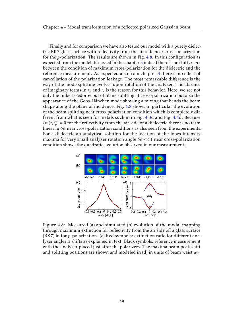
Chapter 4 – Modal transformation of a reflected polarized Gaussian beam
Finally and for comparison we have also tested our model with a purely dielec-tric BK7 glass surface with reflectivity from the air-side near cross-polarizationfor the p-polarization. The results are shown in Fig. 4.8. In this configuration asexpected from the model discussed in the chapter 3 indeed there is no shift α−α0between the condition of maximum cross-polarization for the dielectric and thereference measurement. As expected also from chapter 3 there is no effect ofcancellation of the polarization leakage. The most remarkable difference is theway of the mode splitting evolves upon rotation of the analyzer. The absenceof imaginary terms in rp and rs is the reason for this behavior. Here, we see notonly the Imbert-Fedorov out of plane splitting at cross-polarization but also theappearance of the Goos-Hänchen mode showing a mixing that bends the beamshape along the plane of incidence. Fig. 4.8 shows in particular the evolutionof the beam splitting near cross-polarization condition which is completely dif-ferent from what is seen for metals such in in Fig. 4.3d and Fig. 4.4d. BecauseIm(rsr∗p) = 0 for the reflectivity from the air side of a dielectric there is no termlinear in δα near cross-polarization conditions as also seen from the experiments.For a dielectric an analytical solution for the location of the lobes intensitymaxima for very small analyzer rotation angle δα << 1 near cross-polarizationcondition shows the quadratic evolution observed in our measurement.
Figure 4.8: Measured (a) and simulated (b) evolution of the modal mappingthrough maximum extinction for reflectivity from the air side off a glass surface(BK7) in for p-polarization. (c) Red symbols: extinction ratio for different ana-lyzer angles α shifts as explained in text. Black symbols: reference measurementwith the analyzer placed just after the polarizers. The maxima beam peak-shiftand splitting positions are shown and modeled in (d) in units of beam waist ωf .
49

Chapter 4 – Modal transformation of a reflected polarized Gaussian beam
4.4 Experimental limits, so far
We identify three major limiting factors for the detection performance of ourexperiment; noise, alignment, and the angular resolution in the rotation ofthe polarizers. The cross-polarization extinction is primarily affected by thenoise in photo-detection. We choose to show here the measured intensitiesat cross-polarization with a silver mirror (Fig. 4.9(a)(b)), beam-splitter cube(Fig. 4.9(e)(f)), Bragg mirror (Fig. 4.9(c)(d)) and dielectric BK7 glass surfacereflecting from air (Fig. 4.9(g)(h)) using a logarithmic (a) and linear scale (b). Thelimit of detection is shown in dashed line and will be discussed in this section.
Figure 4.9: A linearly polarized laser beam reflected off a silver mirror (a)(b),(c)(d) Bragg mirror, beam-splitter cube (e)(f) and a glass surface BK7 (g)(h).For all measurements, the cross-polarized intensity is represented in a linearand logarithmic scale for better illustration of the extinction level. The limit ofdetection is shown in dashed line as discussed in text.
In all cases, except results for BK7 glass surface, an extinction beyond alevel 108 is observed. At this point, we can conclude that the challenge in such
50

Chapter 4 – Modal transformation of a reflected polarized Gaussian beam
experiment is to enhance the signal with respect to the noise in photo-detection,known as signal-to-noise ratio. There are numerous sources that generate noisein a photo-diode detector such as thermal noise, shot noise, and dark noise.As a starting point for discussion, we characterize the dark noise in photo-detection which occurs in the absence of a light input. Fig. 4.10 (a) is a plotof the output noise when the laser is completely darkened. The signal is de-tected using an integration time 5 ms namely in a bandwidth ∆f = 200 Hzshows a noise standard deviation given by a root mean square (rms) valueof 107.5 f W , a value comparable to the the manufacturer specification limit84.85 f W (see section 2.2.3). In our case, the maximum intensity obtainedin co-polarization scheme was limited to 233µW . Thus, the noise limit isN = 107.5 f W / 233 µW = 4.61 × 10⁻¹⁰, which corresponds to an extinctionlimit of 1/N = 2.17× 10⁹. One way to improve further the extinction at cross-polarization is the use of a photon counting detectors with a dark noise readoutusually much lower. Another point worth to mention here is that a good align-ment of the setup can definitely lead to an enhancement of the signal-to-noiseratio. The result shown in Fig. 4.10 (b) is a magnification of the cross-polarizedbeam intensity near minimum for a silver mirror (Fig. 4.9(a)(b)). The minimumdetected intensity is I = 156 f W / 233 µW = 6.7× 10⁻¹⁰, a value to be comparedto the dark noise limit N = 4.61× 10⁻¹⁰. This measurement shows that we havereached a record level in the extinction value for which the limiting factor is thedark noise of the detector.
Figure 4.10: (a) The measured output noise without incident light when thelaser is completely darkened using a logarithmic scale. (b) A magnification ofthe cross-polarized beam intensity near minimum for a protected silver mirrorusing a logarithmic scale. The dashed lines refer to the noise limit as discussedin the text.
We now discuss the shot noise limit in photo-detection. This type of noiseis intrinsic to the quantum nature of the source and usually quantified as afunction of the number of photons n that are collected by a given detector perunit of time. The standard deviation of shot noise is equal to the square rootof the n detected photons per second and the signal-to-noise ratio takes theexpression: SNR =
√n. In our case, the detected signal in bright-field is 233 µW
at a wavelength λ = 905 nm, which corresponds to a total energy of n h̄ν with
51

Chapter 4 – Modal transformation of a reflected polarized Gaussian beam
h̄ = h/2π and h is Planck’s constant: 6.626×10⁻³⁴ Joule− sec. Since the energy ofa single photon is h̄ c/λ = 2.19×10⁻¹⁹,we find a number of photons n = 1.06 1015
produced per second. Thus, the signal-to-noise ratio is: SNR =√n = 32× 106,
which we express in photons per square root of Hz. It implies a shot noise7.28 pW /
√∆f = 102.97 pW in a bandwidth ∆f = 200 Hz, a value about 1000
times more than the dark noise limit 107.5 f W . The shot noise due to the laserintensity is almost canceled at cross-polarization condition. In another words,our measurement procedure seems only affected by the dark noise in photo-detection with the exception of thermal noise, usually present in electroniccircuits, that may limit the sensitivity of our photo-detector.
Figure 4.11: Modeled angular resolution as function of the cross-polarizationextinction ratio. The inset is a magnification of the positioning resolution nearmaximum polarization extinction ratio for a linearly polarized beam obtainedby placing the analyzer after a protected silver mirror.
Another point regarding the experimental limits that can be discussed is theangular resolution. The challenge in such experiment is to have a polarizationrotator that enable stepping with small enough rotation angles. To illustratethis point further, we assume a plane wave and a perfect (non leaking) linearpolarizer and analyzer combination. The analyzer is rotated by an angle θwith respect to the polarizer. For such an ideal setup, the detected transmittedintensity (normalized) is
I0 = cos2θ (4.21)
The extinction (ER) is reached for θ =Nπ/2 where N is an integer, this leads toI0 < 1/ER. When ER >> 1 the condition is reached in a range of θ = Nπ/2 − εwhere ε << 1. The goal here is to determine this range of ε given an ER limit.It follows
cos2θ < 1/ER (4.22)
52

Chapter 4 – Modal transformation of a reflected polarized Gaussian beam
This correspond to
sin2 ε << 1/ER (4.23)
Which for ER >> 1 approximates to
ε2 << 1/ER (4.24)
In other words
−1/√ER < ε < 1/
√ER (4.25)
This defines a range ∆ε = 2/√ER, which means that the analyzer rotator resolu-
tion should be better than 2/√ER. To illustrate, in order to reach a systematically
an extinction level of ER = 1010 the resolution should be better than 2×10⁻⁵Rador 1.15×10⁻³deg, the same way to reach ER = 108 the resolution should be betterthan 2×10⁻⁴Rad or 1.15×10⁻²deg. In practice, it is best to work with an angularresolution that is at least a factor 4 better than this limit and this in order to haveenough sensitivity to set comfortably the condition of maximum extinction.Fig. 4.11 is a plot of the angular resolution as a function of the cross-polarizationextinction for which a protected silver mirror is sandwiched between the po-larizer and the analyzer. The extinction enhancement strongly depends on therotation angle and a change of only few mdeg can decrease the extinction inten-sity by one order of magnitude as seen in Fig. 4.11. For our experimental case,we have reached a record level of I0 = 6.7× 10⁻¹⁰ using a piezo rotating stageswith 0.001◦ resolution around the optical axis [45]. This value is comparablewith the theoretical resolution 5.17×10⁻⁵Rad or 3×10⁻³deg. Thus, higher extinc-tion values can only be reached through a piezo rotating stages with additionalprecision specifications. So far, this point has not been further investigated inthis work.
53


Chapter 5
Circular polarization basis: directimaging of Imbert-Fedorov effect in
confocal microscopy
5.1 Motivation
Learning from the previous chapters, we are now moving our exploration to amore fundamental aspect of optics in order to test the predictive ability of themodel and more importantly the experimental power of confocal microscopyto reveal very weak polarization effects. In particular here we want to focus onhow reflecting surfaces affect circularly polarized light. What is well establishedis that a circularly polarized laser beam is reflected with spatial shift transverseto the plane of incidence [19, 20, 22, 33–38]. This Imbert-Fedorov shift, alsoknown as ”spin-Hall effect of light”, was first measured by C. Imbert [20] fora laser beam of circularly polarized light in a glass prism under total internalreflectivity condition (Fig. 5.1(a)(b)). Depending on the chirality of its circularpolarization, the trajectory of a circularly polarized beam will shift above orbelow the plane of incidence when reflected off a surface. This shift is due tospin-orbit coupling of light upon each reflection [21, 38, 46, 47] and is normallyvery small, typically, several orders of magnitude smaller than the photon wave-length. For this reason, it has previously required complex detection schemeslimiting detailed experimental investigations. Here, we report about a novelmethod to measure and map the Imbert-Fedorov shift of Gaussian laser beambased on a dark-field cross-polarization technique in a confocal arrangement.
A considerable amount of literature [42, 48] exists about the measurement ofImbert-Fedorov shift using linear polarization state of light where the reflectedbeam mode splits into two lobes located above and below the reflectivity plane,as already discussed in previous chapters. In our view, this approach is notrelevant to the spin-orbit coupling of light as the notion of a photon spin isusually connected to circular polarization. Because this displacement is perpen-dicular to the plane of reflectivity, the Imbert-Fedorov effect has been renamedas spin-Hall effect of light by authors like Onoda et al. [38], Bliokh et al. [46, 47],
55

Chapter 5 – Circular polarization basis: direct imaging of Imbert-Fedorov effectin confocal microscopy
Aiello et al. [49]. They interpreted the spin-orbit interaction of light in terms ofgeometrical phases and conservation of the total angular momentum of light, asalready predicted by Liberman et al. in 1992 in an inhomogeneous medium [21].More recent evidence of this effect has been shown by Bliokh et al. using multiplereflections in a cylinder glass in which the spin-Hall shift accumulates along ahelical trajectory (Fig. 5.1(c)). In this case, the spin-Hall splitting is amplifiedthrough multiple reflections and becomes noticeable at higher number of turns(Fig. 5.1(d)). In this context, the well-known rotation of the polarization plane fora twisted trajectory is explained based on the Berry phase and the optical Magnuseffect. The first observation of this phenomena in case of metallic reflection wasdemonstrated in [49] by Aiello and his team. In their experiment (Fig. 5.1(e)),they have directly measured the shift of a circularly polarized light instead oflooking at the splitting of a linearly polarized light. The detected shift is in thenanometer range and not measurable at angle of incidence below 50◦ (Fig. 5.1(f)).
Despite the various approaches (Fig. 5.1) that have been developed to inves-tigate the spin-Hall effect of light, this phenomena was not directly observed.It was only measured in some very special situations such as multiple reflec-tions and a weak measurement scheme. This limits the use of this effect asa means for generating, manipulating, and detecting spin-polarized photons.The only evidence so far is a measurement of a polarization-differential shifteither by varying the angle of incidence or the position of the detector. Theuncertainty associated with the measurement of the shift raises many questionsregarding the usefulness and experimental investigation of this effect. In thiswork, we aim to make a mental bridge between all these works and provide aclear explanation of the fundamental origins of the spin-orbit coupling of lightat optical interfaces. For this purpose, we present a mechanical description oftrajectory of a circularly polarized plane wave depending on its orbital angularmomentum. We find a simple formula of the Imbert-Fedorov shift that revealsthe polarization-dependent Hall effect of light previously discussed in literature.Same expression is derived using the full Maxwell approach which is relevant toexplain the important subtleties of phase shifts induced by Fresnel coefficientsupon reflection. We set up a simple, highly reproducible experiment to directlyobserve and measure the Imbert-Fedorov shift for circularly polarized Gaussianbeam. Further measurements of the shift has been carried out using differentangles of incidence θi = 44◦,30◦,21◦,13◦. We discover that a confocal arrange-ment in combination with a dark-field technique amplifies the visibility of theeffect. In addition to new developments in spin-optics systems our experimentsprovide powerful tools to understand spin-orbit coupling of light, in the broadercontext of topological photonics.
56

Chapter 5 – Circular polarization basis: direct imaging of Imbert-Fedorov effectin confocal microscopy
Figure 5.1: (a) Over-all experimental arrangement for measuring Imbert-Fedorovshift in circular polarization state. A laser beam, with horizontal linear polar-ization, traverses a quarter-wave plate and then a half-wave plate covering halfof the beam; the resulting beam, which illuminates the rectilinear object CAB,is thus polarized circularly with opposite helicities on its two halves. This willproduce the differential doubling effect we have alluded to. After illuminatingthe rectilinear object CAB, the beam enters either of our two multiplying prisms,and the image of CAB is finally observed. The high luminosity of the prism Pallows this image to be projected on a screen. (b) Image of a rectilinear objectdisplaying the transverse shift of a circularly polarized beam. The circular polar-ization states of the two halves of the beam are indicated. (See [20] for details).(c) Direct measurement of the spin-Hall of light in a glass cylinder in which theshift accumulates along a helical trajectory. (d) The relative shift between thetwo spin components versus the turns of the helix. (See [47] for details). (e) Theoptical set-up to measure the polarization-differential shift of a beam reflectedoff a thick gold film. (f) Measured polarization-differential shift between σ−/σ+polarized light as function of the angle of incidence. (See [49] for details)
57

Chapter 5 – Circular polarization basis: direct imaging of Imbert-Fedorov effectin confocal microscopy
5.2 Spin and angular momentum of a plane wave
Optical angular momentum is an important concept to get a better understand-ing behind the concept idea of spin-orbit interaction put forward in the liter-ature [38, 46, 47]. In this section, we present an alternative way to explain thetransverse Imbert-Fedorov shift i.e spin-Hall effect of light using the conserva-tion law of the z-component of the total angular momentum upon reflectionat an optical surface. For an idealized circularly polarized plane wave of awavevector ~k0 and momentum ~p, the total angular momentum is expressed as~J = ~Lext + ~S. It consists of the orbital (extrinsic) momentum ~Lext and the spin (in-trinsic) momentum ~S associated with beam trajectory and circular polarization(helicity), respectively. The classical definition of orbital angular momentum perphoton is ~Lext = ~r × ~p where ~r = (∆x,∆y,∆z) is the position vector of the planewave and ~p = h̄~k0, with h̄ = h/2π, h is the Planck’s constant: 6.626 × 10⁻³⁴ J.s.The spin angular momentum per photon is often expressed as ~S = σh̄ ~k0/ |~k0 |,with σ = ±1 for left- and right-handed circularly polarized light respectively andσ = 0 for linearly polarized light.
Figure 5.2: Schematic drawing of a circularly polarized plane wave reflected offan optical surface. The projection of its wavevector ~k0 on the basis (~ex,~ey ,~ez) is(−k0 sinθi ,0, k0 cosθi) where θi is the angle of incidence as explained in text. σinand σout are the polarization helicity state of the incoming and reflected planewave, respectively.
When the plane wave is reflected off an optical interface, the z-component(normal to the surface) of the total angular momentum ~J between the incidentand reflected wave is conserved assuming that the geometric configurationremains unchanged after rotating around the z-axis. The conservation law givesthe following expression: ~S.~ez = ~S ′.~ez +~Lext.~ez, where ~Lext = ~r × ~p is an orbital
58

Chapter 5 – Circular polarization basis: direct imaging of Imbert-Fedorov effectin confocal microscopy
angular momentum with ~p = h̄~k0 and ~r = (∆x,∆y,∆z) an effective orbital radiusto be determined.The conservation equation can be written as h̄k0σin cosθi = −h̄k0σout cosθi +~Lext.~ez, where σin and σout are the polarization helicity state of the incoming andreflected plane wave, respectively. Here,
~Lext = h̄k0
∆x∆y∆z
×−sinθi
0cosθi
(5.1)
By calculating the cross product we can verify that
~Lext = h̄k0
∆y cosθi−∆xcosθi −∆z sinθi
∆y sinθi
(5.2)
Setting up the total angular momentum conservation of the z-component:h̄ σin cosθi = −h̄ σout cosθi +∆y sinθi , leads to an analytical expression for thedisplacement ∆y in a direction perpendicular to the plane of reflection. In acompact form, we show that
∆y =σin + σoutk0 tanθi
(5.3)
This simple equation guides us towards the optimal strategy to perform anexperiment providing the largest ∆y. For an ideal metallic mirror with 100%reflectivity, σout = −σin. This is because a perfect mirror also mirrors the helicityof the polarization meaning that the sum of the spin cancels out σin + σout = 0and there is no shift ∆y above or below the plane of incidence. For a real mirrorsuch as a silver mirror, the sum σin + σout expresses the proportion of minorityphotons that are reflected with the same spin. It is a direct measurement ofthe circular depolarization. A distinctive feature of the shift ∆y is the factthat it is independent of the material properties and beam size of the incidentlight attesting to the robustness of this effect. Because this displacement isperpendicular to the plane of reflectivity, it is also dubbed spin-Hall effectof light. Now the maximum value of ∆y that can be reached is when σout =−σin, which is also σin + σout = 2. This situation can be experimentally realizedby sorting out the majority photons that do not contribute to the maximumsum σin + σout and keep the photon conserving the spin which maximizes thesum. Practically, we use a dark-field cross-polarization technique in a confocalarrangement where a circular analyzer placed on the reflected beam path justto allow the photons with the same helicity as the incoming beam to reach thedetector as explained in section 5.3. In what follows, we evaluate that shift.
59

Chapter 5 – Circular polarization basis: direct imaging of Imbert-Fedorov effectin confocal microscopy
5.3 Confocal imaging of Imbert-Fedorov shift
5.3.1 Experimental setup with circularly polarized light
Figure 5.3: (Left) Experimental setup for measuring and observing the Imbert-Fedorov shift of a circularly polarized laser beam. (Right) Coupling of thelaser source is done in a separate step. Red solid and dashed lines indicate theexcitation and the reflection ray path respectively. See section 2.2.3 for details.
We used the already-introduced confocal arrangement (section 2.2) in orderto emphasize the most relevant physics leading to the Imbert-Fedorov shift of acircularly polarized Gaussian beam reflected off a test mirror. The quarter-waveplates QWP1 and QWP2 allow and reciprocally for conversion of light fromthe linear to the circular or elliptical polarization (or vice versa). We choose azero-order quartz retarders (Thorlabs WPQ05M) with a wavelength 915±35nm,because they offer a lower dependence on temperature and wavelength thanmulti-order wave plates. Each quarter wave-plate is mounted in a continuousrotation mount with adjustable zero (Thorlabs RSP1D ) and an angular reso-lution of 5arcmin Vernier Scale (≈ 0.083◦). In contrast to cross-polarizationextinction measurement, high angular resolution is not a crucial requirement fordetecting the Imbert-Fedorov shift. However, the circular polarizer and analyzerare important optical components for the experiment and the challenge here isto be able to generate circular light with sufficiently high-purity of polarizationstate. In order to provide a direct observation of the beam displacement uponreflection, we mapped the detected intensity by scanning the spatial position ofthe collecting fiber in the focal plane of the focusing objective. We performedsame measurement for different angles of incidence by adjusting the position ofthe reflecting test surface (13) as depicted in Fig. 5.3(left). It is also indispensableto produce high-fidelity imaging of the confocal light and also high-precisionmeasurements of the Imbert-Fedorov shift. In the next section (5.3.2), we ex-
60

Chapter 5 – Circular polarization basis: direct imaging of Imbert-Fedorov effectin confocal microscopy
plain our experimental procedure for generating the circular polarization andmeasuring the beam shift.
5.3.2 Experimental results with circularly polarized light
Figure 5.4: Confocal imaging of a (a) +45◦, (b)−45◦, σ+ and σ− polarized beamoff a test mirror surface in a bright-field (first row) and dark-field (second row)arrangement. We plot the extinction ratio map in logarithmic scale by dividing,pixel per pixel, the bright-field with the dark-field data. In dark-field, a beamshift along ~ey above and below the plane of incidence is observed both forthe σ+ and σ− polarization. The dotted line circle is the 1/e intensity level ofthe Gaussian distribution resulting from the confocal convolution between thefocused spot and the collecting fiber mode. The diameter of this circle gives alsothe non-convoluted focal spot waist diameter at 1/e2 focused on the collectingfiber end. The horizontal white bar represents 5µm.
In our experiment, we use a linear polarizer next to a quarter-wave plateto generate light of circular polarization. We start out by setting the linearpolarizer angle β near 0 for p-polarization (Fig. 5.5(b)) and the linear analyzerangle α near cross-polarization at β ±π/2 (Fig. 5.5(a)). This step is necessaryfor recognizing the p or s reference. The field vector along the p (or s) planeis written as: (1,0) (or (0,1)). Once the maximum extinction is reached, thelinear polarizer (LP) is rotated visually at +45◦ by reading the graduations on
61

Chapter 5 – Circular polarization basis: direct imaging of Imbert-Fedorov effectin confocal microscopy
the Thorlabs manual rotator. The analyzer angle must be then rotated by 90◦
to be set at −45◦ in order to maximize the collected confocal intensity at thedetector i.e bright-field mode (Fig. 5.5(d)). The detected field for +45◦ linearpolarization in a bright-field confocal arrangement is shown in Fig. 5.4(a)(firstrow). To operate in dark-field mode (Fig. 5.5(c)), β remains untouched andwe set the analyzer at the same helicity i.e +45◦ because the mirror flips thesign of the chirality. The detected field in the dark-field mode is shown inFig. 5.4(a)(second row). The measurements in Fig. 5.4(a)(b) show by a factora pure TEM00 Gaussian mode field in bright-field arrangement attenuated by46.79 and 46.83 for +45◦ and −45◦ linearly polarized beam, respectively. Interms of Imbert-Fedorov i.e spin-Hall experiment, we want to come to the mirrorwith a selected photon spin and measure after the mirror the number of photonsthat made it out to the detector with the exact same spin. For this case, weplace a first quarter-wave plate (QWP1) after the linear polarizer (LP) at +45◦
and before the mirror. The QWP1 is mounted on a Thorlabs rotator in a waythat its fast axis is along the p plane (i.e. horizontal in our setup). In this case,the linearly polarized light beam has an angle of +45◦ with the fast axis, thephase shift will be π/2 between polarization components and the out-going lightbeam is circularly polarized. When the linear polarization is parallel to thefast axis, there is no phase shift and no change in the polarization state. Next,the second quarter-wave plate (QWP2) is added after the mirror and before thelinear analyzer (LA). Since the mirror flips the chirality of the beam, we usethe combination {QWP2, LA +45◦} and {QWP2, LA −45◦} to switch betweendark-field and bright-field modes as illustrated by Fig. 5.5(e) and (f) respectively,assuming a left-hand incident circular polarization σ+ i.e {LP +45◦, QWP1}. Inthe same way, we define the combination {QWP2, LA −45◦} and {QWP2, LA+45◦} to switch between dark-field and bright-field modes respectively in case ofright-hand circular polarization σ− i.e {−45◦ LP, QWP1}.
To get a feel of the measured Imbert-Fedorov shift for a circular polariza-tion σ+ and σ− at an angle of incidence θi = 44◦, we measured and showedin Fig. 5.4(c)(d) the confocal light intensity in a bright-field and dark-field ar-rangement(Fig. 5.5(f)(e)). We observed that the reflected beam spot measured indark-field arrangement is displaced perpendicularly to the plane of incidence.The peak-shift occurs along ~ey and located above or below the reflectivity planefor σ+ and σ− polarization, respectively. The measured subwavelength shiftshowed in Fig. 5.6 is yσ+
= +330nm and yσ− = −340nm when switching betweencircular polarization σ+ and σ−. Thus, the total displacement is ∆y = 670nm.This is consistent with the value 2× (λ/π)cotθi = 596nm, calculated using theexpression (5.3) for a simple plane wave reflected of a silver mirror at θi = 44◦
and λ = 905nm. In this dark-field configuration, we find an extinction ratio47.59 and 47.86 for σ+ and σ− polarization, respectively. Here, it is worth tomention that the measured extinction ratio for σ+ and σ− have almost a valuesimilar to the value for +45◦ and −45◦ linearly polarized beam, respectively. Thisreflects the fact that quarter-wave plates aligned along its fast or slow axis donot reduce the intensity of the incident ±45◦ incident light, as it passes through it.
62

Chapter 5 – Circular polarization basis: direct imaging of Imbert-Fedorov effectin confocal microscopy
Figure 5.5: Measurement protocol for observation of the Imbert-Fedorov shiftupon reflection. First we set a linear p-polarization in (b) co-and (a) cross-polarization scheme, respectively. Next, the linear polarizer is rotated at +45◦.For the bright-field arrangement the linear polarizer (LP) and the lineare analyzer(LA) are set up in parallel (d) while for the dark-field arrangement they arerotated by 90◦. Two quarter-wave plates QWP1 and QWP2 are then addeddirectly before and after the mirror, respectively. The fast axis of both wave-plates is parallel to p plane. In this geometry, the dark-field and bright-fieldarrangement are shown in (e) and (f), respectively. To measure the shift in theopposite direction, the polarizer is rotated by 90◦ in a dark-field arrangement asshown in (g). Then, the analyzer is rotated also by 90◦ to switch to bright-fieldmode as illustrated in (h).
63

Chapter 5 – Circular polarization basis: direct imaging of Imbert-Fedorov effectin confocal microscopy
The first important condition for the success of our experiment is the stabilityof the maxima beam position during the confocal imaging process. Keeping thisin mind, we present in Fig. 5.4(first row) the confocal imaging in a bright-field ar-rangement, where the location of the maxima of the beam lie exactly on the circleindicating the 1/e intensity level of the Gaussian distribution. This indicates thatour setup is mechanically stable and not affected by any drift problem whichleads to moving the beam maxima location. We have also experimentally verifiedthe stability and the reproducibility of the shift on the reflected confocal spotunder different incidence angles for instance θi = 30◦, 21◦, 13◦ attesting to the ro-bustness of this effect. We observed similar behavior for all the mentioned anglesof incidence, with the difference that the value shift is amplified while decreasingthe incidence angle as already predicted from expression 5.3: 2 × (λ/π)cotθi .Corresponding experimental results are shown and discussed in section 5.4.Here we show results for 29◦ as depicted in Fig. 5.6. In this case, the shift isyσ+
= +680± 0.04nm and yσ− = −680± 0.04nm when switching between a polar-ization σ+ and σ−, respectively. These values are comparable to the calculatedvalue using the plane wave model (λ/π)cotθi = 520nm, with λ = 905nm. Thedifference could be possibly related to the purity of the polarization state of light.
Figure 5.6: Measured and calculated circularly polarized laser beam reflected offa silver mirror in a dark-field confocal arrangement for θi = 29◦ incidence angle.The bright-field beam (black circles) is centered in the middle with maximumintensity 160µW . The measured intensity profiles for σ+ and σ− polarizationare shown using red and white circles, respectively. The measured shift isyσ+
= +680± 0.04nm and yσ− = −680± 0.04nm when switching between circularpolarization σ+ and σ−, respectively.
The challenge in this experiment towards proving the existence of such sub-wavelength shift is to check the purity of the generated circular polarizationby combination of the linear polarizer and the quarter-wave plate (QWP1). Aquarter-wave plate has two principal axes: fast and slow. Each axis has a differentrefractive index and, therefore, a different wave velocity. If the light after thelinear polarizer is at ±45◦ and the quarter-wave plate is aligned at an angle otherthan the fast or slow axis, then the output will be elliptically polarized. Thus,the knowledge of the fast or slow axis of the quarter-wave plate is crucial for
64

Chapter 5 – Circular polarization basis: direct imaging of Imbert-Fedorov effectin confocal microscopy
manipulating the polarization state of light beams. It is worth to mention herethat the output light from a quarter-wave plate aligned along the fast or slowaxis is left or right-hand circular polarization. The commercial quarter-waveplates we used in this work had already the fast axis denoted by a line. Oth-erwise, it may be found out easily by verifying that the dark-field intensity onthe detector decreases by 1/2 as compared to a p or s polarization. In fact, thenormalized field intensity in the dark-field confocal arrangement for +45◦ linearpolarization is given by equation (3.6) for β = π/4 and α = π/4. This is expressedby: I = |rp + rs|2/4. First thing to note from this formula is that the sum rp + rsgoverns the dark-field detected field intensity. Later in the analysis (section 5.5)we will see that this sum appear as pre-factors in the description of circularlypolarized reflected fields.
ERmeasured ERtheory θi ∆measured ∆ref erence
47.73± 0.15 93.37 44◦ 98.32◦ ± 0.02◦ 95.94◦
(2.53± 0.03)× 102 4.96× 10² 30◦ 93.60◦ ± 0.02◦ 92.57◦
(1.16± 0.01)× 103 2.18× 10³ 21◦ 91.68◦ ± 0.01◦ 91.23◦
(1.02± 0.04)× 104 1.52× 10⁴ 13◦ 90.57◦ ± 0.02◦ 90.46◦
Table 5.1: Overview of the measured extinction ratio ERmeasured and phase dif-ference ∆measured for different incidence angles θi = 44◦,30◦,21◦,13◦. Referencevalues of ERref erence and ∆ref erence are determined from [28].
It is worth emphasizing that an ideal mirror i.e rp = 1 and rs = −1 reversesthe chirality of the photon meaning that rp + rs = 0. For high reflectivity mate-rials such as silver mirror, we have rp + rs = 2cos∆ where ∆ = (φp −φs)/2 is thephase difference (see section 3.2 for more details). The significant result fromthe formula of the detected field in dark-field arrangement is the fact that theextinction ratio 1/I = 4/ |rp + rs|2 which is also 1/(cos2∆), is a direct measurementof the purity of the generated circular polarization as reported in table 5.1. Wehave measured the extinction ratio in a dark-field configuration for differentangles of incidence θi = 44◦,30◦,21◦,13◦. In particular, a good agreement be-tween theoretical and experimental values is found, highlighting the highestpurity of circular polarization. We have also determined the correspondingphase difference ∆measured for each θi = 44◦,30◦,21◦,13◦. In fact the incidenceangles are deduced from the measurement of the extinction ratio. In practical,we set a rough nominal incidence angle θi , then compare the measured (ER) tothe reference value reported from literature [28] for silver and then we deduce
65

Chapter 5 – Circular polarization basis: direct imaging of Imbert-Fedorov effectin confocal microscopy
the exact value of θi . This technique used for measuring the phase difference∆ = (φp −φs)/2 is a simple way for incidence angle calibration in a variety ofhigh-precision measurement in polarimetry and micro-ellipsometry. In con-clusion, the significant results in table 5.1 report on a robust method based ondark-field confocal arrangement to directly measure and check the purity of thepolarization state of light taking advantage on the effect that light reflected by ametallic surface introduces a phase shift between the p and s components of thebeam due to the Fresnel reflectivity coefficients rp and rs.
5.4 Measurements at different angles of incidence
Figure 5.7: Rough way to set the incidence angle θi . It is measured usinga tangent function tan2θi = IM2/IM1 in the triangle (IM1M2). The distanceIM2 remains unchanged and only the distance IM2 is adjusted by horizontaltranslation of the test mirror in order to vary the angle of incidence θi of thelaser beam. An exact measurement of incidence angle θi is finalized through ERmeasurements as discussed in text.
Following equation 5.3 for plane wave the Imbert-Fedorov shift is expected toevolve as cotgθi , in other words we are compelled to explore the smaller anglesregion. Here, we were interested in observing the shift at angles of incidenceθi = 44◦,30◦,21◦,13◦. In practice, we have setup four different experimentsgiven a specific θi angle setting. In particular, the test mirror is moved relativeto the incident light beam to change the angle between the beam and the testsurface mirror. The reflected beam travels off at an angle of reflection which isequal to the angle of incidence according to the law of reflection. The angle ofincidence is predicted by a tangent function as depicted in Fig. 5.7.For each incidence angle θi setting, we have mapped the confocal light intensity,for σ+ and σ− circular polarization, measured in a bright-field (Fig. 5.8) anddark-field (Fig. 5.9) arrangement, respectively. Only half beam is shown foreach circular polarization for better illustration of the direct observation of theImbert-Fedorov shift. In all cases, the bright-field intensity profile is essentially
66

Chapter 5 – Circular polarization basis: direct imaging of Imbert-Fedorov effectin confocal microscopy
a reminiscent of a TEM00 Gaussian beam for σ+ and σ− polarization, respectively.The location of the peak intensity is centered at 0, there is no maxima positiontechnical spurious drift of the laser beam during the confocal scanning processwhich might be caused by poor mechanical mounting of the optomechanicalparts or upon rotation of optical components such as the quarter-wave plate.These measurements (Fig. 5.8) are intended to evaluate the beam-positioningperformance of our setup as well as examine the fidelity and long-term stabilityover 24 hours, of the Imbert-Fedorov shift measured in the dark-field confocalarrangement. We have experimentally verified the stability of the beam maximaposition θi = 44◦,30◦,21◦,13◦ as depicted in Fig. 5.8(e)(f)(g)(h) attesting to therobustness of the experimental setup.
Figure 5.8: Bright-field measurements in a confocal arrangement for incidenceangles θi = 44◦(a)(e),30◦(b)(f ),21◦(c)(g),13◦(d)(h) when using σ+ and σ− circularpolarization. The measurements demonstrate that no technical spurious shiftsaffect our experimental setup in configurations for which no measurable shift isexpected. Only half beam is shown for each circular σ+ and σ− polarization. Themeasured intensity profiles for σ+ (red circles) and σ− (white circles) polarizationare shown in the lower row.
We now discuss the results in Fig. 5.9 where the confocal light intensity forσ+ and σ− circular polarization is measured in dark-field arrangement. Themost striking result to emerge from the data Fig. 5.9(a)(b)(c)(d) is that theImbert-Fedorov shift i.e spin-Hall effect is amplified as the angle of incidence θidecreases. This finding confirms the initial calculations of conservation of totalangular momentum for a simple circularly polarized plane wave reflecting offa metallic mirror (section 5.2). In our measurement procedure of the shift, weuse the least-squares method to fit a Gaussian model to our experimental data.The beam shift yσ± is measured with a fitting error between the experimentalvalues and those given by the fitted curve. Our measurements of the Imbert-Fedorov shift for σ+ and σ− circular polarization are summarized in table 5.3.
67

Chapter 5 – Circular polarization basis: direct imaging of Imbert-Fedorov effectin confocal microscopy
Figure 5.9: Analysis of the Imbert-Fedorov shift for σ+ and σ− polariza-tion in a dark-field confocal arrangement for incidence angles settings θi =44◦(a)(e),30◦(b)(f ),21◦(c)(g),13◦(d)(h). Only half beam is shown for each circu-lar σ+ and σ− polarization. The measured intensity profiles for σ+ (red circles)and σ− (white circles) polarization are shown in the lower row.
There is no significant differences between the measured ∆ymeasured = yσ+ − yσ−and calculated ∆yplanewave = 2 × (λ/π)cotθi total displacement of the oppositeshifts of the two circular polarizations in case of θi = 44◦,30◦,21◦,13◦ incidenceangles. It is worth to mention here that the data at 13◦ is no longer explainedby the simplistic model of plane wave. To the best of our knowledge, we arethe first to now see the departure from the divergence given by the plane waveapproximation for low angles of incidence. The agreement with Gaussian modelis excellent as we will discuss later in this chapter.
At this point, we were able to directly observed the Imbert-Fedorov shift incase of metallic reflection through the use of dark-field confocal arrangement.Specifically, we used a powerful technique based on cross-polarization measure-ment to filter away photons that are not experiencing spin-orbit coupling uponreflectivity. So far, all the presented experimental results except for θi = 13◦
are in good agreement with the simple argument that for a plane wave theconservation of the projection of angular momentum along the mirror normalaxis (i.e. mirror rotation invariance around that axis) the wave is displacedperpendicularly to the plane of incidence. This cannot be measured for a planewave as it has an infinite extend and therefore its location cannot be defined.However for a finite sized beam, such a Gaussian beam, we have shown that thisshift is clearly observable. In what follows we uncover the physics responsiblefor Imbert-Fedorov shift for a Gaussian beam and we will explain convincinglyall the features of the measured results.
68

Chapter 5 – Circular polarization basis: direct imaging of Imbert-Fedorov effectin confocal microscopy
θi yσ− yσ+ ∆ymeasured ∆yplanewave
44◦ −340± 0.03nm +330± 0.03nm 670nm 596nm
30◦ −500± 0.02nm +520± 0.03nm 1.02µm 997nm
21◦ −710± 0.01nm +710± 0.02nm 1.42µm 1.50µm
13◦ −1050± 0.02nm +1040± 0.02nm 2.09µm 2.49µm
Table 5.2: Overview of the measured Imbert-Fedorov shift for different inci-dence angles θi = 44◦,30◦,21◦,13◦. For each θi angle setting, we measure theImbert-Fedorov shift for σ+ and σ− circular polarization. ∆ymeasured = yσ+ − yσ−corresponds to the total displacement of the opposite shifts of the two circularpolarizations. The theoretical value of ∆yplanewave = 2× (λ/π)cotθi is determinedforλ = 905nm as explained in text (see section 5.2 for details ).
5.5 Imbert-Fedorov shift for a circularly polarizedGaussian beam
Figure 5.10: Geometry of beam reflection off a mirror. The incident beam hasa Gaussian field distribution in the transverse plane. The transverse u, v andlongitudinal w wavenumbers depend on the angle of incidence as explained inprevious chapter.
We assume an incoming laser beam circularly polarized reflected off a metal-lic mirror (see Fig. 5.10). We express the result conveniently using the matrixformalism, already introduced in previous chapter. The resulting normalized
69

Chapter 5 – Circular polarization basis: direct imaging of Imbert-Fedorov effectin confocal microscopy
reflected field is expressed as follows:
~ENorm = exp(−x2
0 + y20
2ω2f
)¯̄Aσ±
¯̄MDx0,y0¯̄Pσ±~Ep (5.4)
We recall that the mirror reflectivity matrix (including confocal Gaussian filter-ing) is given by equation (4.9):
¯̄MDx0,y0=
[rp 00 rs
]+ i
x0
2lf
[r ′p 00 r ′s
]+ i
y0
2lf
rp + rstanθi
[0 −11 0
](5.5)
where r ′p/s = ∂rp/s/∂θi is the first order derivative of Fresnel coefficients withrespect to the angle of incidence θi . The matrix of a circular polarizer/analyzeris given by (Appendix G):
¯̄Pσ± = ¯̄Aσ± =12
[1 ∓i±i 1
](5.6)
Applying such a matrix on a linearly polarized field along ~p gives
¯̄Pσ±~Ep =1√
2
1√
2
[1 ∓i±i 1
][10
](5.7)
which is also
¯̄Pσ±~Ep =1√
2
1√
2
[1±i
](5.8)
The matrix product above of linearly polarized field along ~p followed by a leftor right circular polarizer produces ~σ+ or ~σ− circularly polarized field. It isstraightforward to verify that:
~ENorm =1√
2
(rp + rs√2±
y0√2lf
rp + rstanθi
+ ix0√2lf
(rp + rs)′
2
)exp −
(x20 + y2
0
2ω2f
)~σ± (5.9)
where r ′p/s = ∂rp/s/∂θi is the first order derivative of Fresnel coefficients withrespect to the angle of incidence θi . Therefore,
~ENorm =rp + rs
2
(1±
y0
lf
1tanθi
+ ix0
lf
(rp + rs)′
2(rp + rs)
)exp
(−x2
0 + y20
2ω2f
)~σ± (5.10)
This is the detected field of a confocal scanning microscope in a circular polar-ization dark-field arrangement normalized to the bright-field value at confocalaperture placed at the origin. Equation (5.10) provides the general form of theconfocal dark-field mapping of a Gaussian beam reflected off a material surface(dielectric or metallic). The assymetric modal distribution along y0 is clearlyaffected by the chirality of the light polarization the focus of this chapter. Theassymetric field distribution along x0 is directly proportional to dispersion of
70
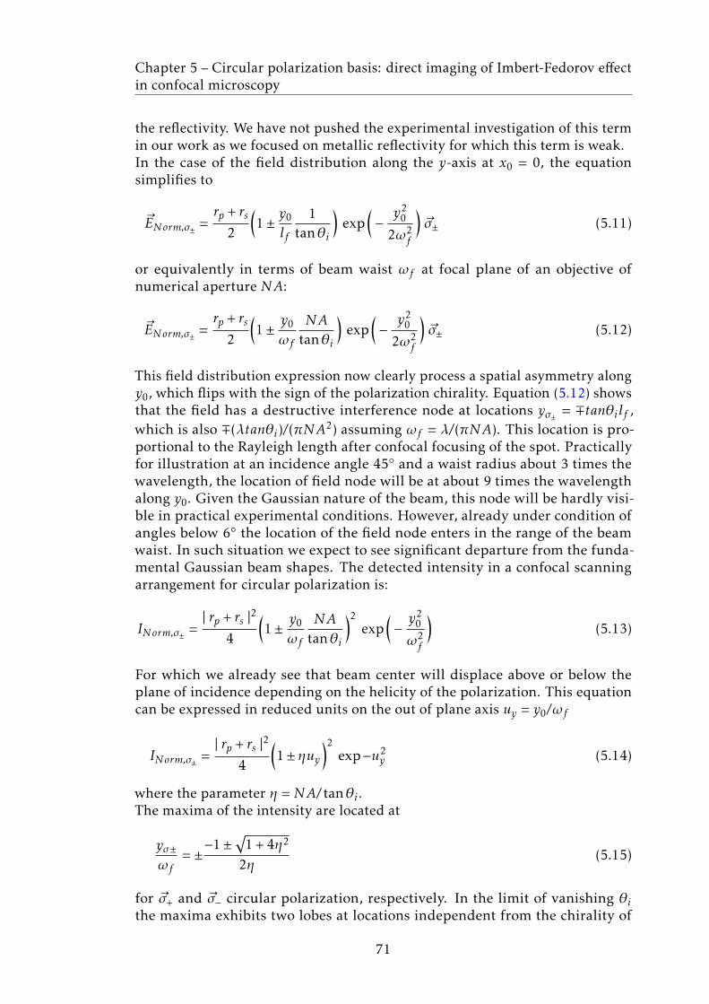
Chapter 5 – Circular polarization basis: direct imaging of Imbert-Fedorov effectin confocal microscopy
the reflectivity. We have not pushed the experimental investigation of this termin our work as we focused on metallic reflectivity for which this term is weak.In the case of the field distribution along the y-axis at x0 = 0, the equationsimplifies to
~ENorm,σ± =rp + rs
2
(1±
y0
lf
1tanθi
)exp
(−y2
0
2ω2f
)~σ± (5.11)
or equivalently in terms of beam waist ωf at focal plane of an objective ofnumerical aperture NA:
~ENorm,σ± =rp + rs
2
(1±
y0
ωf
NAtanθi
)exp
(−y2
0
2ω2f
)~σ± (5.12)
This field distribution expression now clearly process a spatial asymmetry alongy0, which flips with the sign of the polarization chirality. Equation (5.12) showsthat the field has a destructive interference node at locations yσ± = ∓tanθilf ,which is also ∓(λtanθi)/(πNA2) assuming ωf = λ/(πNA). This location is pro-portional to the Rayleigh length after confocal focusing of the spot. Practicallyfor illustration at an incidence angle 45◦ and a waist radius about 3 times thewavelength, the location of field node will be at about 9 times the wavelengthalong y0. Given the Gaussian nature of the beam, this node will be hardly visi-ble in practical experimental conditions. However, already under condition ofangles below 6◦ the location of the field node enters in the range of the beamwaist. In such situation we expect to see significant departure from the funda-mental Gaussian beam shapes. The detected intensity in a confocal scanningarrangement for circular polarization is:
INorm,σ± =| rp + rs |2
4
(1±
y0
ωf
NAtanθi
)2exp
(−y2
0
ω2f
)(5.13)
For which we already see that beam center will displace above or below theplane of incidence depending on the helicity of the polarization. This equationcan be expressed in reduced units on the out of plane axis uy = y0/ωf
INorm,σ± =| rp + rs |2
4
(1± ηuy
)2exp−u2
y (5.14)
where the parameter η =NA/ tanθi .The maxima of the intensity are located at
yσ±ωf
= ±−1±
√1 + 4η2
2η(5.15)
for ~σ+ and ~σ− circular polarization, respectively. In the limit of vanishing θithe maxima exhibits two lobes at locations independent from the chirality of
71

Chapter 5 – Circular polarization basis: direct imaging of Imbert-Fedorov effectin confocal microscopy
the circular polarization, namely at ±ωf independently of the sign of the po-larization. In other words, the intensity has two maxima along a line perpen-dicular to the plane of incidence in a way identical to the case of p or s beamin cross-polarization. In the limit of NA << tanθi , for instance for very wideGaussian beam waist, the dominant maximum is located at ±NA/ tanθi for the~σ+ and ~σ− circular polarization. We see therefore that the corresponding lo-cation yσ± = ±(λ/π)cotθi as expected for a plane wave. In fact, in this limit ofNA << tanθi this shift is independent from the Gaussian beam size. Thus, the ex-pression yσ± = ±(λ/π)cotθi , which is also ωf (NA/tanθi) define the experimentalcondition for which the spin-orbit interaction of light can be made very clearlyvisible. The full measurements shown in Fig 5.11 are fitted using the formula ofmaxima of the intensity for a Gaussian beam (full line) and plane wave (dashedline) in units of beam waist radius ωf . It shows first that the shift is alwayssmaller than the beam waist. Nevertheless, it will still be many orders of magni-tudes larger than in bright-field experiments without an analyzer. Worse stillthe bright-field experiment with a circular analyzer gives a 0 shift as expectedfrom the conservation of angular momentum analysis. To illustrate the case, weconsider NA = 0.115, taking an angle of incidence of 20◦ we will get a separationof beam position the order 63% of the beam radius when switching between apositive to a negative chirality of the circular polarization, as shown in Fig 5.11.Such a large visibility of the effect is unprecedented and is of text-book quality(see Fig 5.11).
θi yσ− yσ+ y/ωf yplanewave yGaussian
44◦ −340± 0.03nm +330± 0.03nm ±0.117 ±298nm ±294nm
30◦ −500± 0.02nm +520± 0.03nm ±0.191 ±498nm ±480nm
21◦ −710± 0.01nm +710± 0.02nm ±0.27 ±750nm ±693nm
13◦ −1050± 0.02nm +1040± 0.02nm ±0.413 ±1.24µm ±1.03µm
Table 5.3: Overview of the measured Imbert-Fedorov shift for different inci-dence angles θi = 44◦,30◦,21◦,13◦. For each θi angle setting, we measure theImbert-Fedorov shift for σ+ and σ− circular polarization. ∆ymeasured = yσ+ − yσ−corresponds to the total displacement of the opposite shifts of the two circularpolarizations. The theoretical value of ∆yplanewave = 2× (λ/π)cotθi is determinedfor λ = 905nm as explained in text (see section 5.2 for details).
72

Chapter 5 – Circular polarization basis: direct imaging of Imbert-Fedorov effectin confocal microscopy
Figure 5.11: Measured Imbert-Fedorov shift for σ± circular polarization in unitof beam waist radius ωf in case of silver mirror and for a laser wavelengthλ = 905nm. We plot the position of intensity maxima for a plane wave (dashedline) and Gaussian beam (full line) reflected off a silver mirror as a function ofpolarization excitation and detection. σ± Dark-field and σ± Bright-field denotethe dark-field (σ±Mσ±) and bright-field (σ±Mσ∓) configurations respectively,when the mirror (M) is sandwiched between two circular polarizers. The datameasured at θi = 13◦ shows clearly the departure from the plane wave approxi-mation divergence (dashed line) for low angles of incidence. The Gaussian beammodel is in a very good agreement (full line).
5.6 Imbert-Fedorov shift without the use of polar-ization analyzer
The "original" Imbert-Fedorov shift, namely circularly polarized reflected Gaus-sian beam without the use of polarization analyzer configuration the field distri-bution in a confocal arrangement is given by removing the analyzer function inequation (4.10)
~ENorm(x0, y0) = ¯̄MDx0,y0¯̄Pσ±~Ep (5.16)
where ¯̄Pσ± is the Jones matrix of a circular polarizer (see Appendix G). We recallthat the mirror reflectivity matrix (including confocal Gaussian filtering) is givenby equation (4.9):
¯̄MDx0,y0=
[rp 00 rs
]+ i
x0
2lf
[r ′p 00 r ′s
]+ i
y0
2lf
rp + rstanθi
[0 −11 0
](5.17)
The job to be done in this configuration is to evaluate the ¯̄M1¯̄Pσ± ~Ep, ¯̄M2
¯̄Pσ± ~Epand ¯̄M3
¯̄Pσ± ~Ep. Where
73

Chapter 5 – Circular polarization basis: direct imaging of Imbert-Fedorov effectin confocal microscopy
¯̄M1¯̄Pσ±~Ep =
1√
2
1√
2
[rp 00 rs
][1 ∓i±i 1
][10
](5.18)
this
¯̄M1¯̄Pσ±~Ep =
1√
2
1√
2
[rp±irs
](5.19)
Moving to the next term gives a very similar calculation
¯̄M2¯̄Pσ±~Ep = i
x0
2lf
1√
2
1√
2
∂∂θi
[rp±irs
](5.20)
The last term involves an anti-diagonal matrix
¯̄M3¯̄Pσ±~Ep = i
y0
2lf
rp + rstanθi
1√
2
1√
2
[0 −11 0
][1 ∓i±i 1
][10
](5.21)
this
¯̄M3¯̄Pσ±~Ep = i
y0
2lf
rp + rstanθi
1√
2
1√
2
[0 −11 0
][1±i
](5.22)
The next term is
¯̄M3¯̄Pσ±~Ep = i
y0
2lf
rp + rstanθi
1√
2
1√
2
[∓i1
](5.23)
Giving
¯̄M3¯̄Pσ±~Ep = ±
y0
2lf
rp + rstanθi
1√
2
1√
2
[1±i
](5.24)
Now putting all terms together, we get
~ENorm =12
exp(−x2
0 + y20
2ω2f
) rp + i x02lf
∂rp∂θi± y0
2lf
rp+rstanθi
±i(rs + i x0
2lf∂rs∂θi± y0
2lf
rp+rstanθi
) (5.25)
Case x0 = 0
~ENorm =12
exp(−x2
0 + y20
2ω2f
) rp ±y02lf
rp+rstanθi
±i(rs ±
y02lf
rp+rstanθi
) (5.26)
74

Chapter 5 – Circular polarization basis: direct imaging of Imbert-Fedorov effectin confocal microscopy
The corresponding intensity is
INorm =14
exp(−y2
0
ω2f
)(| rp |2 + | rs |2 +2
∣∣∣∣ y0
2lf
rp + rstanθi
∣∣∣∣2 + 2y0
2lf
|rp + rs|2
tanθi
)(5.27)
Compare this to the case with a circular analyzer in dark-field (see equation(5.10))
INorm,σ± =| rp + rs |2
4exp
(−y2
0
ω2f
) (1±
y0
lf
1tanθi
)2(5.28)
which is also
INorm,σ± =| rp + rs |2
4exp
(−y2
0
ω2f
) (1 + |
y0
lf
1tanθi
|2 ± 2y0
lf
1tanθi
)(5.29)
Both equations for the case with and without an analyzer show a similar an-alytical expression. This said, clearly, the weight of the polarization chiralitydependent terms (i.e linear in y0) in the measurement without analyzer is re-duced by a factor |rp + rs|2/4. So in limit in which the quadratic term in y0 doesnot dominate the line shape (i.e away from vanishing angle of incidence), wecan directly deduce the Imbert-Fedorov shift from our previous calculation forthe dark-field case (see section 5.5) for the positive and the negative circularpolarization.We see therefore that the corresponding locations are given by:
ymax± ≈ ±| rp + rs |2
4λ
π tanθi(5.30)
Very much like in the dark-field confocal configuration (section 5.5), the shiftis independent from the size of the beam. The notable difference is that nowthe shift depends on the material optical properties through |rp + rs|2. For silverthe calculated pure Imbert-Fedorov shift is shown in the table 5.4. This is to becompared to the dark-field measurement in circular polarization.
Note the connection to the extinction ratio |rp + rs|2/4 = 1/(ER) which showsthat in the dark-field configuration the Imbert-Fedorov shift is amplified by ER.The question remains to demonstrate formally whether or not this "amplification"of the shift obtained by sorting out the photons not experiencing spin-orbitinteraction is the same as the one found from the general frame work of theweak-measurement technique [42]. The fact that the amplification factor isdirectly given by the extinction ratio is a strong indication that the principle ofweak measurement is not applying to this case. This said, the special situationof dark-field measurement for the very particular case of circular polarization
75

Chapter 5 – Circular polarization basis: direct imaging of Imbert-Fedorov effectin confocal microscopy
θi ymax± without analyzer yσ± in dark-field
44◦ 3.20nm 335nm
30◦ 1.01nm 510nm
21◦ 0.035nm 710nm
13◦ 0.08nm 1.045nm
Table 5.4: Overview of the Imbert-Fedorov shift for different incidence anglesθi = 44◦,30◦,21◦,13◦ without analyzer and in dark-field configuration. Foreach θi incidence, the shift is calculated for σ+ and σ− circular polarization atλ = 905nm as explained in text.
(and away from the low angle limit) is that the Imbert-Fedorov shift does notdepend on the material property but solely on the photon polarization chiralityproperties, its wavelength and its angle of incidence. This is not the case forany other polarization state. It is very interesting to note that for this verypure circular polarization configuration, the shift is free from the arbitrarinessinherent to the weak measurement technique, namely that the amplificationfactor can be in principle set to any arbitrary value. We verified indeed thataway from a pure circular polarization state of the polarizer and analyzer wecould measure a massive amplification that we could simply set by choosing thedegree of ellipticity of our polarization.
76

Chapter 5 – Circular polarization basis: direct imaging of Imbert-Fedorov effectin confocal microscopy
5.7 Remark
Literature about spin-Hall effect of light has tended to confirm that a simplemirror reflectivity splits a linearly polarized Gaussian beam into left and rightcircularly polarized beams [42]. Such unjustified postulation can lead to seriousquestions regarding the nature of the polarization state of the Imbert-Fedorovmodes observed previously in this work for a linearly polarized beam. In thiscontext, we now assume that we manage to make an experiment that bringthe fields ~ENorm,σ± (section 5.5) to add or substract interferometrically. Thisexperiment requires splitting the incoming beam in two parallel fields of twoopposing circular polarization, each beam then is reflected and passes twoindividual circular polarization analyzers of same chirality of the correspondingimpinging beam. Finally both beams need to be combined on a detector. Arather complex procedure but let us see what would be the result. In this casewe make use of the linear combination of fields
~p =(~σ+ + ~σ−)√
2(5.31)
~s = −i (~σ+ − ~σ−)√2
(5.32)
We recall that:
~ENorm,σ± =rp + rs√
2
(1±
y0
lf
1tanθi
)exp−
( y20
2ω2f
)~σ± (5.33)
We see that if we just added or subtracted the fields
~ENorm,σ++ ~ENorm,σ−√2
=rp + rs
2exp
(−x2
0 + y20
2ω2f
) ( ~σ+ + ~σ−√2
+y0
lf
1tanθi
~σ+ − ~σ−√2
)(5.34)
Like wise
~ENorm,σ+− ~ENorm,σ−√2
=rp + rs
2exp
(−x2
0 + y20
2ω2f
) ( ~σ+ − ~σ−√2
+y0
lf
1tanθi
~σ+ + ~σ−√2
)(5.35)
Now we conveniently express both fields in terms of ~p and ~s
~ENorm,σ++ ~ENorm,σ−√2
=rp + rs
2exp
(−x2
0 + y20
2ω2f
) (~p+ i
y0
lf
1tanθi
~s)
(5.36)
and
~ENorm,σ+− ~ENorm,σ−√2
=rp + rs
2exp
(−x2
0 + y20
2ω2f
) (i~s+
y0
lf
1tanθi
~p)
(5.37)
77

Chapter 5 – Circular polarization basis: direct imaging of Imbert-Fedorov effectin confocal microscopy
We see clearly that any linear combination of this form will not allow tohave a cancellation of intensity on axis at y0 = 0. More generally, any linearcombination a~ENorm,σ+
+ b~ENorm,σ− adding the fields (even with complex coeffi-cients) terms will not lead to a cancellation of the intensity at y0 = 0. To get acancellation of the field at y0 = 0, we need instead to pass the combined fieldsthrough a linear crossed polarizers that ends up keeping just the terms in y0.In this very complicated configuration, we recover the results obtained simplyusing a pair of linear polarizer and analyzer. The message here is to tell thatsumming up the fields do not lead to a pure linearly polarized beam.
5.8 Conclusion
In conclusion we presented a novel method to measure and map the Imbert-Fedorov shift based on a dark-field cross-polarization technique in a confocalarrangement. In our proposed dark-field configuration under circular polariza-tion, the majority photons reflected off a surface that are not contributing tothe shift are filtered-out. The minority photons possess the proper chirality forspin-orbit coupling of light enabling this way the magnification of the Imbert-Fedorov shift by several orders of magnitudes. We verified that the out of planeof incidence shift measured this way is a direct consequence of the conservationof total angular momentum. Building on our detailed model for Gaussian laserbeams derived for the first part of this work we have verified quantitativelyexperimentally that the shift increases significantly when decreasing the angleof incidence, this, to the best of our knowledge, is a novel regime that was notexplored previously. The analytical model show an excellent agreement withour measurements performed on a silver mirror. In particular, the model re-veals clearly a regime of lower angle of incidence below which the simplisticapproach of quasi plane wave would lead to an unphysical divergence of theshift at vanishing angles. In such a low angle regime, our model eliminates thisshift divergence and predicts instead a modal transformation of the reflectedminority photons to the next higher Hermite-Gaussian modes in a way verysimilar to that explored in the first part of this work. First data indicate thetransition into such a regime.
78

Chapter 6
Summary and perspectives
Our study provides a robust toolbox for a new way to do fluorescence spec-troscopy and polarimetry experiments using confocal microscopy. We haveexposed a systematic experimental method based on a confocal microscopyarrangement to obtain a giant enhancement in dark-field cross-polarization ex-tinction and this by up to 3 orders of magnitudes and possibly beyond. Wefound that the effect exploits the material properties of a surface or interfaceunder condition of total internal reflectivity in particular. In more general terms,the effect was found to be fully governed by the phase difference, such as in-duced by beam-splitter cubes and Bragg mirrors, between the reflectivity oflight components polarized in and out of plane of incidence. Now that the basicprinciple of cancellation of polarization leakage is established, there are optionsfor improving the experimental detection limit of the cross-polarization extinc-tion ratio. First it is possible to improve the signal-to-noise ratio. Generally, itis helpful to increase the optical input power by better alignment. However,this depends primarily on the application. In some cases, noisy lasers can’t bestabilized and a suitable type and model of photo-detector can (and cannot)improve the signal-to-noise ratio. Second possibility is to amplify the rotation-angle precision. It is demonstrated in chapter 4 that a positioning resolution of10−6 degrees allows measuring an extinction ratio value in the level of 1011 andbeyond. It is practically possible to obtain a sub-step-size rotation resolutionwith selected attocube controllers. An already existing solution is the bearingbased rotator ECR4040/Al/NUM/RT with an integrated 1/2" aperture, suitablefor optical experiments. It is designed for ambient conditions with a fine angularposition of 0.04m◦.
Furthermore, we have also presented the theoretical modal analysis of beamreflectivity. In fact, modeling this effect led us to simulate and map in minutedetails the transformation of Gaussian beams near cross-polarization into Imbert-Fedorov higher modes, a physics governed essentially by the finite divergence ofa Gaussian beam reflecting off a surface. Results so far have been very promisingup to first order transformation in x and y. One potential promising applicationof our approach would be to simulate and map the transformation of Gaussianbeams at higher order modes. So far we did not observe any trace of the mode
79

Appendix – Summary and perspectives
TEM11 signal. There is no doubt however that this mode is present as measuredin [43], this is why we believe that our model is not complete yet. Future workshould also concentrate on enhancing the quality of the extinction ratio in areal-world confocal device made of several mirrors and beam-splitter cubes indifferent and complex geometries. We are confident that our model will serve asa base for setting up the basic building block of any future optical spectroscopysystem. The present model is based on a pure Maxwell plane wave expansionapproach. The next step is to include the connection between the Imbert-Fedoroveffect and geometric phases. This is absolutely essential in the conception anddesign of modern spin-based optical devices.
In chapter 5, we have presented a direct observation of the Imbert-Fedorovshift i.e spin-Hall effect for spin up and down of light (circular polarization).This was never seen clearly in a text book. We have demonstrated that theImbert-Fedorov like it is said in text books that (i) a laser beam shifts out of theplane of specular incidence when the light is impinging in a circular polariza-tion and detected in the same circular polarization. (ii) The sign of the shift isgiven by the chirality. This is a new finding in microscopy and can lead to somemeasurement issues or opportunities for researcher doing measurements undercircular polarization. We showed both theoretically and experimentally, thatthe effect is a consequence of conservation of total angular momentum betweenthe incident and reflected beam. To be convincing, we have also verified themaxima beam position stability of our setup. The idealized situation of a circularpolarized plane wave light and a highly reflective perfect mirror is perfectlypredictive, namely it predicts a displacement shift typically dependent on theco-tangent of incidence angle cotθi . This beautiful result comes from a verysimple calculation that consider the conservation of angular momentum of lightprojected on the z-axis perpendicular to the mirror. In this work and in real-lifemicroscopy experiments we ask ourselves how does that apply to a Gaussian fo-cused beam in a confocal configuration. To answer this we have made our modelcalculations first in the limit of smaller NA and found the exact same result forthe shift of location of the maximum of the beam intensity. So we now have aregime for which a Gaussian mode appear to act like a plane wave. We verifyour theory by experimental measurements at difference incidence angles. Ourexperimental approach has a number of similarities with the weak measurementtechnique, the main difference is that we measure at exact cross-polarizationcondition. Further experimental investigations are needed to understand theorigin of the weak measurement amplification of the shift already reported inliterature [42, 48]. This is an important matter for future research.
This work opens the way to methodical design of sensitive laser resonantfluorescence microscopes with extreme background extinction, for a broad rangeof applications in quantum optics and solid-state physics. The new methodsdeveloped for this work can also be applied for measuring material opticalproperties and polarimetry applications.
80

Appendix A
Supplementary information tochapter 3
“The physical origins of cancellationof polarization leakage”
The purpose of this section is to derive an expression for the cross-polarizationextinction amplification in a confocal arrangement. For this purpose, we assumean incoming laser field ~Ep initially p-polarized that we rotate at an angle β
aligning it with the polarizer such ~E(β) = ¯̄R(β)~Ep. This field first traverses theleaky polarizer also rotated at β such ¯̄P (β) = ¯̄R(β) ¯̄L ¯̄Pp0
¯̄R(−β) followed by themirror matrix ¯̄M and by the analyzer matrix rotated at an angle α namely¯̄A(α) = ¯̄R(α) ¯̄L ¯̄Ap0
¯̄R(−α) so the field ~E just after the analyzer writes
~E = ¯̄A(α) ¯̄M ¯̄P (β) ¯̄R(β)~Ep (A.1)
A.1 Jones calculus
To calculate equation (A.1), we start first by performing a simple matrix multi-plication of the Jones matrix of the input laser field together with the polarizerat an angle β. We find that
¯̄P (β) ¯̄R(β)~Ep = ¯̄R(β) ¯̄L ¯̄Pp0¯̄R(−β) ¯̄R(β)~Ep (A.2)
Here the product ¯̄R(−β) ¯̄R(β) is equal to identity matrix. Thus, we can write
⇔ ¯̄P (β) ¯̄R(β)~Ep = ¯̄R(β) ¯̄L ¯̄Pp0~Ep
We recall that the incoming laser field ~Ep is initially p-polarized i.e ~Ep =[10
],
¯̄L ¯̄Pp0=
[a 0−ib 0
]and ¯̄R(β) =
[cosβ −sinβsinβ cosβ
]. Therefore,
81

Appendix A – Supplementary information to chapter 3“The physical origins of cancellation of polarization leakage”
⇔ ¯̄P (β) ¯̄R(β)~Ep =[cosβ −sinβsinβ cosβ
] [a 0−ib 0
] [10
]Now we calculate the matrix product
⇔ ¯̄P (β) ¯̄R(β)~Ep =[cosβ −sinβsinβ cosβ
] [a−ib
]which is also
⇔ ¯̄P (β) ¯̄R(β)~Ep =[acosβ + ib sinβasinβ − ibcosβ
](A.3)
For a high quality commercially available polarizers a2 >> b2. Thus a2 ≈ 1 andthe leakage b2 is in the range of 105 and 106 in best cases. A practical check forp- polarized light, namely β = 0 leads to the expected field vector [1, ib] at theoutput of a leaky polarizer along ~p.Now, let’s calculate the matrix of a leaky analyzer rotated at α defined as:
¯̄A(α) = ¯̄R(α) ¯̄L ¯̄Ap0¯̄R(−α) (A.4)
Using ¯̄L ¯̄Ap0= ¯̄L ¯̄Pp0
=[a 0−ib 0
]and ¯̄R(α) =
[cosα −sinαsinα cosα
], we can write that
¯̄A(α) =[cosα −sinαsinα cosα
] [a 0−ib 0
] [cosα sinα−sinα cosα
](A.5)
Here, the matrix product calculation leads to
⇔ ¯̄A(α) =[cosα −sinαsinα cosα
] [acosα asinα−ibcosα −ib sinα
]So after simplifying, this expression becomes:
⇔ ¯̄A(α) =[acos2α + ibcosα sinα acosα sinα + ib sin2αacosα sinα − ibcos2α asin2α − ibcosα sinα
](A.6)
which can be also written as:
⇔ ¯̄A(α) =[a ib−ib a
][cos2α cosα sinα
cosα sinα sin2α
](A.7)
From equation (A.7), we note that the matrix of a real physical linear analyzeris none than a combination of an ideal linear polarizer at an angle α and theleakage Jones matrix ¯̄L.
82

Appendix A – Supplementary information to chapter 3“The physical origins of cancellation of polarization leakage”
A.2 Expression of the electric field after the ana-lyzer (equation (3.4))
We introduce Eq. (A.3) and Eq. (A.7) into Eq. (A.1) , the electric field after theanalyzer can be therefore written as
~E = ¯̄A(α) ¯̄M ¯̄P (β) ¯̄R(β)~Ep (A.8)
By inserting equation (A.7) and equation (A.3) into equation (A.8), we obtain
~E =[a ib−ib a
][cos2α cosα sinα
cosα sinα sin2α
][rp 00 rs
] [acosβ + ib sinβasinβ − ibcosβ
]The matrix product calculation leads to
~E =[a ib−ib a
][cos2α cosα sinα
cosα sinα sin2α
] [rp(acosβ + ib sinβ)rs(asinβ − ibcosβ)
]which is also
~E =[a ib−ib a
] [rp(acosβ + ib sinβ)cos2α + rs(asinβ − ibcosβ)cosα sinαrp(acosβ + ib sinβ)cosα sinα + rs(asinβ − ibcosβ)sin2α
]So after simplifying, this expression becomes:
~E ={rp(acosβ + ib sinβ)cosα + rs(asinβ − ibcosβ)sinα
}[a ib−ib a
] [cosαsinα
]Finally,
~E ={rp(acosβ+ ib sinβ)cosα+ rs(asinβ− ibcosβ)sinα
} [acosα + ib sinα−ibcosα + asinα
](A.9)
A.3 Expression of the light intensity after the ana-lyzer (equation (3.6))
The corresponding intensity is determined by I =| ~E |2, which is also
I =∣∣∣∣rp(acosβ + ib sinβ)cosα + rs(asinβ − ibcosβ)sinα
∣∣∣∣2 (A.10)
with | acosα+ib sinα |2 + | −ibcosα+asinα |2= a2 +b2 = 1. Equation (A.10) reads
I =∣∣∣∣arp cosβ cosα + ars sinβ sinα + ibrp sinβ cosα − ibrs cosβ sinα
∣∣∣∣2 (A.11)
We calculate the product of the electric field after the analyzer and its complexconjugate, we obtain
83

Appendix A – Supplementary information to chapter 3“The physical origins of cancellation of polarization leakage”
I = a2 | rp cosβ cosα + rs sinβ sinα |2 +b2 | rp sinβ cosα − rs cosβ sinα |2 +K1 +K2
where
K1 =(arp cosβ cosα + ars sinβ sinα
)(ibrp sinβ cosα − ibrs cosβ sinα
)∗or
K1 = −iabrpr∗p cosβ sinβ cos2α − iabrsr∗p sin2β sinα cosα
+iabrpr∗s cos2β sinα cosα + iabrsr
∗s cos2β sin2α
and
K2 =(arp cosβ cosα + ars sinβ sinα
)∗(ibrp sinβ cosα − ibrs cosβ sinα
)or
K2 = iabrpr∗p cos2β cos2α + iabr∗s rp sin2β sinα cosα
−iabr∗prs cos2β sinα cosα − iabrsr∗s cos2β sin2α
We calculate the sum K1 +K2, we obtain
K1 +K2 = iabrpr∗s cosα sinα − iabrsr∗p cosα sinα = iabcosα sinα(rpr
∗s − rsr∗p)
which is also
K1 +K2 = −2abIm(rpr∗s )cosα sinα (A.12)
Inserting K1 and K2 into equation (A.11) leads to
I = a2 | rp cosβ cosα + rs sinβ sinα |2 +b2 | rp sinβ cosα − rs cosβ sinα |2
− 2abIm(rpr∗s )cosα sinα
(A.13)
A.4 Angular shift as a function of Fresnel reflectioncoefficients
To get a better feel for the relevant parameters in canceling almost perfectlythe polarization leakage we use the form rp = ρp exp(iϕp) and rs = ρs exp(iϕs)that can be conveniently symmetrized using ρs = ρ+ δρ/2, ρp = ρ − δρ/2 for thereflectivity and ∆ = (ϕp −ϕs)/2 the phase difference. This way we obtain
¯̄M =[rp 00 rs
]= e−i∆
[(ρ − δρ/2)ei∆ 0
0 (ρ+ δρ/2)e−i∆
](A.14)
84

Appendix A – Supplementary information to chapter 3“The physical origins of cancellation of polarization leakage”
For high reflectivity mirrors ρp ≈ ρs ≈ 1 and δρ = 0
¯̄M ≈[ei∆ 00 e−i∆
](A.15)
Thus, the Fresnel reflection coefficients can be approximated by rp ≈ ei∆ andrs ≈ e−i∆.We recall that the light intensity just after the analyzer is given by equation(A.10):
I =| rp(acosβ + ib sinβ)cosα + rs(asinβ − ibcosβ)sinα |2
Inserting rp and rs into the expression of the intensity
I =| ei∆(acosβ + ib sinβ)cosα + e−i∆(asinβ − ibcosβ)sinα |2 (A.16)
In case of a perfect leakage cancellation, i.e I = 0
I = 0⇔| ei∆(acosβ + ib sinβ)cosα + e−i∆(asinβ − ibcosβ)sinα |2= 0
This means that the real and the imaginary parts of I are both equal to 0 and weobtain a set of two equationsacosβ cosα cos∆− b sinβ cosα sin∆+ asinβ sinα cos∆− bcosβ sinα sin∆ = 0acosβ cosα sin∆+ b sinβ cosα cos∆− asinβ sinα sin∆− bcosβ sinα cos∆ = 0
(A.17)
Using the identities cos(α ∓ β) = cosα cosβ ± sinα sinβ andsin(α ∓ β) = sinα cosβ ∓ cosα sinβ, we can rewrite equation (A.17)acos∆cos(α − β) = b sin∆sin(α + β)asin∆cos(α + β) = bcos∆sin(α − β)
(A.18)
If we divide the first equation of the system (A.18) by acos∆ and second one bybcos∆, we getcos(α − β) = b
a tan∆sin(α + β)sin(α − β) = a
b tan∆cos(α + β)(A.19)
To solve this system of two equations, both equations are multiplied by the factorab and we define the sum of their squares as
a2b2(cos2(α − β) + sin2(α − β)) = tan2∆(b4 sin2(α + β) + a4 cos2(α + β)) (A.20)
Using cos2(α − β) + sin2(α − β) = 1 and a2 + b2 = 1, we get
a2b2 = tan2∆(b4 sin2(α + β) + (1− b2)(1− b2)cos2(α + β))
85

Appendix A – Supplementary information to chapter 3“The physical origins of cancellation of polarization leakage”
which is also
⇔ a2b2 = tan2∆(b4 sin2(α + β) + (1 + b4 − 2b2)cos2(α + β))
After simplification, we get
⇔ a2b2 = tan2∆(b4 sin2(α + β) + b4 cos2(α + β) + (1− 2b2)cos2(α + β))
From cos2(α + β) + sin2(α + β) = 1, we obtain
⇔ a2b2 = tan2∆(b4 + (1− 2b2)cos2(α + β)) (A.21)
Using equation (A.21), we express cos(α + β) as
cos(α + β) =1
tan∆
b√
1− 2b2
√a2 − b2 tan2∆ (A.22)
In our case a = 1 and b << 1, therefore√
1− 2b2 ≈ 1,√a2 − b2 tan2∆ ≈
√a2 = a = 1
and
cos(α + β) =b
tan∆(A.23)
Therefore,
sin(α + β) =
√1− b2
tan2∆(A.24)
Inserting Eq. (A.23) and Eq. (A.24) into the system of equation (A.19), we getcos(α − β) = ba tan∆sin(α + β)
sin(α − β) = ab tan∆cos(α + β)
which is also
⇔
cos(α − β) = ba tan∆
√1− b2
tan2∆
sin(α − β) = a
Finally, the solution of the system of equation (A.19) is given bycos(α − β) = b tan∆
sin(α − β) = 1(A.25)
Now, we want to extract the values of α and β from equation (A.25). For thisreason, we use the definition of the analyzer angle α = π
2 + ε in case of mirrormeasurement at cross-polarization :
cos(α − β) = b tan∆⇔ cos(π
2+ ε − β
)= b tan∆
86

Appendix A – Supplementary information to chapter 3“The physical origins of cancellation of polarization leakage”
Using the identity cos(A+B) = cosAcosB− sinAsinB, we obtain
⇔ cos(π
2
)cos(ε − β)− sin
(π2
)sin(ε − β) = b tan∆
Thus
⇔−sin(ε − β) = b tan∆
In the approximation of small angles sin(ε − β) = (ε − β):
⇔−(ε − β) = b tan∆
We recall that α = π2 + ε, therefore
⇔ β +π2−α = b tan∆ (A.26)
In case of no mirror measurement, the analyzer angle α0 is related to the polarizerangle β by the following expression: α0 −β = π
2 . Moreover, we define a system ofequation for mirror/no mirror measurement as:α − β = π
2 ∓ b tan∆
α0 − β = π2
which reduces to
⇔ α −α0 = ∓b tan∆ (A.27)
with α and α0 are the analyzer angle for mirror/no mirror measurement atcross-polarization for a given polarizer angle β.
A.5 Maximum acceptable limit of polarization leak-age
In this part, we would like to get an accurate value of the polarization leakageb2. We recall equation (A.21): a2b2 = tan2∆(b4 + (1− 2b2)cos2(α + β)).Using a2 + b2 = 1, we obtain
b2 − b4 = tan2∆(b4 + (1− 2b2)cos2(α + β)) (A.28)
For the sake of simplification, we consider A = tan2∆ usually A >> 1 and x =cos2(α + β). Therefore,
b2 − b4 = A(b4 + (1− 2b2)x) (A.29)
We write the equation (A.29) in form of a polynomial function in b,
⇔ b4(1 +A)− b2(1 + 2Ax) +Ax = 0 (A.30)
87

Appendix A – Supplementary information to chapter 3“The physical origins of cancellation of polarization leakage”
We divide equation (A.30) by the factor 1 +A and we get:
⇔ b4 − b2 1 + 2Ax1 +A
+Ax
1 +A= 0 (A.31)
Now, let us study the possible solutions for this equation. One could show that:
b2 =12
{1 + 2Ax1 +A
±
√(1 + 2Ax)2
(1 +A)2 −4Ax1 +A
}which is also
⇔ b2 =12
1 + 2Ax1 +A
{1±
√1− 4Ax(1 +A)
(1 + 2Ax)2
}(A.32)
There are no solutions for b when the term under the square root is < 0, so wemust have
1− 4Ax(1 +A)(1 + 2Ax)2 > 0 (A.33)
We multiply the equation (A.33) by the factor (1 + 2Ax)2
⇔ (1 + 2Ax)2 > 4Ax(1 +A)
This defines the range of xmax which can be determined by the solving thefollowing equation
⇔ (1 + 2Ax)2 − 4Ax(1 +A) = 0 (A.34)
Using the identity (u + v)2 = u2 + 2uv + v2, we get
⇔ 1 + 4A2x2 + 4Ax − 4Ax(1 +A) = 0 (A.35)
We write the equation (A.35) in form of a polynomial function in x,
⇔ 4A2x2 + (4A− 4A− 4A2)x+ 1 = 0 (A.36)
We divide equation (A.38) by the factor 4A2 and we obtain:
⇔ x2 +−4A2
4A2 x+1
4A2 = 0
which is also
⇔ x2 − x+1
4A2 = 0 (A.37)
The two possible solutions of equation (A.37) arexmax+ = 1
2
{1 +
√1− 1
A2
}xmax− = 1
2
{1−
√1− 1
A2
} (A.38)
88

Appendix A – Supplementary information to chapter 3“The physical origins of cancellation of polarization leakage”
When (1 + 2Ax)2 − 4Ax(1 +A) = 0, equation (A.32) becomes
⇔ b2 =12
1 + 2Ax1 +A
(A.39)
Therefore, the possible values of b2 are given by:b2max+ = 1
21+2Axmax+
1+Ab2max− = 1
21+2Axmax−
1+A
(A.40)
Inserting equation (A.37) into equation (A.40) we getb2max+ = 1
2
(1 +
√A−1A+1
)b2max− = 1
2
(1−
√A−1A+1
) (A.41)
Recalling that A = tan2∆, finallyb2max+ = 1
2
(1 +
√tan2∆−1tan2∆+1
)b2max− = 1
2
(1−
√tan2∆−1tan2∆+1
) (A.42)
89


Appendix B
Supplementary information tochapter 4
“Modal transformation of a reflectedpolarized Gaussian beam”
B.1 Reflection matrix as a function of (u,v) (equa-tion (4.3))
Figure B.1: Geometry of beam reflection off a mirror. The incident beam hasa Gaussian field distribution in the transverse plane. The transverse u, v andlongitudinal w wavenumbers depends on the angle of incidence as explained inprevious chapter.
Here we use the general wave propagation convention exp(ikr − iωt). Weconsider that the finite size beam before the mirror results from a Gaussianweighted superposition of plane waves propagating along an angular distribu-tion ~k/k0 = u~p+ v~s+w~k0/k0 narrowly centered around ~k0 with k0 = 2π/λ whereu, v and w are angular variables along ~p, ~s and ~k0/k0 respectively. For each planewave component, we choose a coordinate system ~ep, ~es, ~k/k0 that defines a local
incidence plane for that wave. The longitudinal basis vector is ~k/k0 and the
91

Appendix B – Supplementary information to chapter 4“Modal transformation of a reflected polarized Gaussian beam”
transverse ones are ~es =~k/k0 ×~ez and ~ep = (~k/k0 ×~ez)× (~k/k0) in the s and p planes
respectively. We now express these vectors in the coordinate system ~p, ~s, ~k0/k0 asdepicted below
Figure B.2: Schematic illustration of reflection geometry. ~k/k0 = u~p+v~s+w~k0/k0
is the wavenumber vector with ~k0 with k0 = 2π/λ and u, v and w are angularvariables along ~p, ~s and ~k0/k0 respectively.
Therefore,
−→es =~k/k0×~ez =
uvw
×sinθi
0cosθi
=
v cosθi−u cosθi +w sinθi
−v sinθi
(B.1)
and
−→ep = (~k/k0 ×~ez)× (~k/k0) =
v cosθi−u cosθi +w sinθi
−v sinθi
×uvw
we calculate the cross product of the two vectors
=
w(−u cosθi +w sinθi)− v2 sinθi−vwcosθi −uv sinθi
(u2 + v2)cosθi −uw sinθi
(B.2)
In the paraxial limit u,v << θi , we can write
−→es = sinθi
v cotθi−u cotθi +w
−v
≈v cotθi
1−v
(B.3)
and
−→ep = sinθi
−u cotθi +w2 − v2
−vwcotθi −uv(u2 + v2)cotθi −uw
≈ 1−v cotθi−u
(B.4)
To obtain the reflectivity of the mirror for each plane wave, we determine firstthe weights of p- and s- field-components, given by the weighted projectionsrp,uv(~ep · ~E0uv) and rs,uv(~es · ~E0uv). We determine then the resulting reflected field
92

Appendix B – Supplementary information to chapter 4“Modal transformation of a reflected polarized Gaussian beam”
transverse field along the corresponding reflected basis ~es,R = ~kR/k0 × ~ez and~ep,R = (~kR/k0 ×~ez)× (~kR/k0) such ~Euv = rp,uv(~ep · ~E0uv)~ep,R + rs,uv(~es · ~E0uv)~es,R. Here~kR is the mirrored wave vector after reflection. In the paraxial limit, for a beamimpinging, the Fresnel coefficients are developed to the first order in u aroundθi and v around 0, giving: rp,uv = rp + u ∂rp/∂θi and rs,uv = rs + u ∂rs/∂θi . Thefirst order derivatives ∂rp/s uv/∂v in the s-plane vanish both for rp and rs leavingjust derivative r
′p = ∂rp/∂θi and r
′s = ∂rs/∂θi . We calculate the components of the
reflected basis vectors ~ep,R, ~es,R, ~kR in the paraxial limit u,v << θi .Therefore, we obtain
~ep,R = −→ep (−u,v,π −θi) ≈
1v cotθiu
(B.5)
and similarly we get
~es,R = −→es (−u,v,π−θi) ≈
−v cotθi1−v
(B.6)
Inserting equation (B.3), (B.4), (B.5) and (B.6) into ~Euv we obtain
~Euv = rp,uv(~ep·~E0uv)~ep,R+rs,uv(~es·~E0uv)~es,R (B.7)
For simplicity, we only calculate the components along ~p and ~s of equation (B.7)
~Euv = rp,uv([
1−v cotθi
]·[EpEs
])[1
v cotθi
]+rs,uv
([v cotθi
1
]·[EpEs
])[−v cotθi1
](B.8)
Calculating first the scalar product terms (~ep · ~E0uv) and (~es · ~E0uv),
~Euv = rp,uv(Ep − v cotθiEs)[
1v cotθi
]+ rs,uv(v cotθiEs +Ep)
[−v cotθi
1
](B.9)
then we have
~Euv =[
rp,uv(Ep − v cotθiEs)v cotθirp,uv(Ep − v cotθiEs)
]+[−v cotθirs,uv(v cotθiEs +Ep)
rs,uv(v cotθiEs +Ep)
](B.10)
which is also
~Euv =[rp,uv(Ep − v cotθiEs)− v cotθirs,uv(v cotθiEs +Ep)v cotθirp,uv(Ep − v cotθiEs) + rs,uv(v cotθiEs +Ep)
](B.11)
Inserting rp,uv = rp +u ∂rp/∂θi and rs,uv = rs +u ∂rs/∂θi into equation (B.11), weget
~Euv =[(rp +u ∂rp/∂θi)(Ep − v cotθiEs)− v cotθi(rs +u ∂rs/∂θi)(v cotθiEs +Ep)v cotθi(rp +u ∂rp/∂θi)(Ep − v cotθiEs) + (rs +u ∂rs/∂θi)(v cotθiEs +Ep)
]93

Appendix B – Supplementary information to chapter 4“Modal transformation of a reflected polarized Gaussian beam”
Up to the first order in u and v, the reflected field vector is then given by:
~Euv =[rpEp +uEp ∂rp/∂θi −Esrpv cotθi −Esrsv cotθiEprpv cotθi +Eprsv cotθi + rsEs +uEs ∂rs/∂θi
](B.12)
After simplification, we can write
~Euv =[rpEp +uEp ∂rp/∂θi −Es(rp + rs)v cotθirsEs +uEs ∂rs/∂θi +Ep(rp + rs)v cotθi
](B.13)
Using r ′p/s = ∂rp/s/∂θi in equation (B.13) , we obtain
~Euv =[rpEp +uEp r ′p −Es(rp + rs)v cotθirsEs +uEs r ′s +Ep(rp + rs)v cotθi
](B.14)
We express the result in terms of matrix notation in the standard ~p, ~s basis suchthat
~Euv = ¯̄Mu,v~E0uv
where
~Euv =[
rp +ur ′p −v cotθi(rp + rs)v cotθi(rp + rs) rs +ur ′s
][EpEs
](B.15)
One can conclude that
¯̄Mu,v =[
rp +ur ′p −v cotθi(rp + rs)v cotθi(rp + rs) rs +ur ′s
](B.16)
It is convenient to write separately the components of equation (B.16) dependingon u and v variables in order to discuss the modal transformation of the incidentbeam. Thus,
¯̄Mu,v =[rp 00 rs
]+u
[r ′p 00 r ′s
]+ v
rp + rstanθi
[0 −11 0
](B.17)
B.2 Reflected field distribution in the (x,y) domain(equation (4.4))
To calculate the expression of the reflected beam detected after the lens, we needto derive the field distribution that result when we focus a particular far-fieldonto an image plane. To get a better feeling we assume the lens is illuminated bya plane wave field ~E(u,v) traveling along ~k at an angle u,v off a given optical axisof a lens as depicted below. A surface element of a focusing lens such dS = dxdycause a field density at location (x′, y′). This field is caused by the plane wave at
94

Appendix B – Supplementary information to chapter 4“Modal transformation of a reflected polarized Gaussian beam”
Figure B.3: Focusing of a plane wave into a point as explained in text. f is thefocal length. ~k wavevector at an angle u,v. dS = dxdy a surface element of afocusing lens
angle u,v so it will be indexed such as: Eu,v(x′, y′). Here we use the general wavepropagation convention exp(ikr − iωt). Fresnel-Huygens principle dictate thateach point of the surface element dS emit coherently as a single point emitter.
The total field caused at (x′, y′) due to the plane wave E(u,v) field densityover the area dS is therefore:
+∞"−∞
Eu,v(x′, y′)dx′ dy′ = α
+∞"−∞
E(u,v)exp+i~k ·~r|~r |
dxdy (B.18)
where α is a normalization constant to be calculated. Fresnel-Huygens principlecan be easily treated in a paraxial approximation here for which the largestcontribution of the field at (x,y) causing a field at (x′, y′) are due to the locationof the surface such x << f , y << f . So we can expand
r2 = f 2 + x2 + y2 = f 2(1 +x2 + y2
f 2 ) (B.19)
In the paraxial approximation x << f and y << fwe can show that:
|~r | ≈ f +x2 + y2
2f(B.20)
replacing |~r | in we get
+∞"−∞
Eu,v(x′, y′)dx′ dy′ = αE(u,v)exp(ikf )
f
+∞"−∞
exp+ikx2 + y2
2fdxdy (B.21)
here E(u,v) being a plane wave field density does not depend on (x,y). Also inour approximation we have taken the denominator |~r | ≈ f . Now physically the
full field at (x′, y′) namely+∞!−∞Eu,v(x′, y′)dx′ dy′ is caused by the full field E(u,v)
of the plane wave. So we have
95

Appendix B – Supplementary information to chapter 4“Modal transformation of a reflected polarized Gaussian beam”
|~r | ≈ f +x2 + y2
2f(B.22)
replacing |~r | in we get
+∞"−∞
Eu,v(x′, y′)dx′ dy′ = αE(u,v)exp(ikf )
f(B.23)
making use of equation (B.23) in (B.21) we get
1 =αf
+∞"−∞
exp+ikx2 + y2
2fdxdy (B.24)
using a first identification R2 = x2 + y2, the integral becomes
1 =αf
2π∫0
+∞∫0
exp+ikR2
2fRdRdψ (B.25)
which is also
1 = 2πα
+∞∫0
exp+ikR2
2f2RdR
2f(B.26)
making second identification −W = ikR2/2f , we get
−dWik
=2RdR
2f(B.27)
which is also
idWk
=2RdR
2f(B.28)
Using the above formula in the integral we get
1 =2παik
+∞∫0
(exp−W )dW (B.29)
which is also
1 =2παik
(B.30)
96

Appendix B – Supplementary information to chapter 4“Modal transformation of a reflected polarized Gaussian beam”
since k = 2π/λ, we finally get 1 ≈ αiλ. Thus, α = −i/λ.
In our case, we consider the propagation of a Gaussian field angular dis-tribution (source plane) indicated by the coordinate variables u and v. At thesource plane, the area dS = dudv defines the extent of the beam. The fielddistribution in the source plane is given by Eu,v(u,v) and the field ~Ef x,y(x,y) inthe observation plane. Now back to equation B.18, in the paraxial approximationwe have:
~Ef x,y(x,y) =−iλ
+∞"−∞
Eu,v(u,v)exp+ i~k ·~r|~r |
dudv (B.31)
Here ~k/k0 = u~p + v~s +w~k0/k0 narrowly centered around ~k0 with k0 = 2π/λ and~r = x~p+ y~s is the distance between a position on the source plane and a positionin the observation plane. Thus, we obtain:
~Ef x,y(x,y) =−iλf
exp(+ik0f )
+∞"−∞
Eu,v(u,v) exp[+ik0(xu + yv)]dudv (B.32)
In what follows, we will drop the phase term exp+ik0f as we are interested toexpress the field in the focal region.
B.2.1 p-polarization
In our case a p-polarized light is obtained at β = 0 and its corresponding cross-polarization is reached when α = π/2. For simplicity, we calculate the reflectivityof a p-polarized beam at cross-polarization in case of a = 1 and b = 0. We recallthat the reflected field distribution after the mirror for each angle u,v
~Euv = ¯̄A(α) ¯̄Mu,v¯̄P (β)~E0uv (B.33)
where
¯̄Mu,v =[rp 00 rs
]+u
[r ′p 00 r ′s
]+ v
rp + rstanθi
[0 −11 0
](B.34)
and
~E0uv =E0
πθ20
exp(− u
2 + v2
θ20
)[cosβsinβ
](B.35)
When β = 0 and α = π/2, ¯̄A(α) =[0 00 1
]and ¯̄P (β) =
[1 00 0
]. Therefore, we find
that
~Euv =E0
πθ20
exp(−u
2 + v2
θ20
)[0 00 1
][rp +ur ′p −v cotθi(rp + rs)
v cotθi(rp + rs) rs +ur ′s
][1 00 0
][10
](B.36)
97
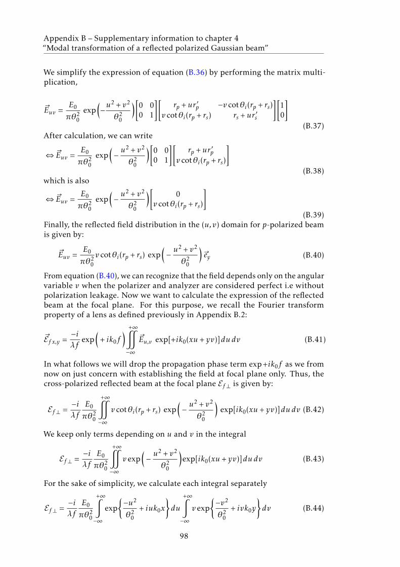
Appendix B – Supplementary information to chapter 4“Modal transformation of a reflected polarized Gaussian beam”
We simplify the expression of equation (B.36) by performing the matrix multi-plication,
~Euv =E0
πθ20
exp(−u
2 + v2
θ20
)[0 00 1
][rp +ur ′p −v cotθi(rp + rs)
v cotθi(rp + rs) rs +ur ′s
][10
](B.37)
After calculation, we can write
⇔ ~Euv =E0
πθ20
exp(− u
2 + v2
θ20
)[0 00 1
][rp +ur ′p
v cotθi(rp + rs)
](B.38)
which is also
⇔ ~Euv =E0
πθ20
exp(− u
2 + v2
θ20
)[ 0v cotθi(rp + rs)
](B.39)
Finally, the reflected field distribution in the (u,v) domain for p-polarized beamis given by:
~Euv =E0
πθ20
v cotθi(rp + rs) exp(− u
2 + v2
θ20
)~ey (B.40)
From equation (B.40), we can recognize that the field depends only on the angularvariable v when the polarizer and analyzer are considered perfect i.e withoutpolarization leakage. Now we want to calculate the expression of the reflectedbeam at the focal plane. For this purpose, we recall the Fourier transformproperty of a lens as defined previously in Appendix B.2:
~Ef x,y =−iλf
exp(
+ ik0f) +∞"−∞
~Eu,v exp[+ik0(xu + yv)]dudv (B.41)
In what follows we will drop the propagation phase term exp+ik0f as we fromnow on just concern with establishing the field at focal plane only. Thus, thecross-polarized reflected beam at the focal plane Ef ⊥ is given by:
Ef ⊥ =−iλf
E0
πθ20
+∞"−∞
v cotθi(rp + rs) exp(− u
2 + v2
θ20
)exp[ik0(xu + yv)]dudv (B.42)
We keep only terms depending on u and v in the integral
Ef ⊥ =−iλf
E0
πθ20
+∞"−∞
v exp(− u
2 + v2
θ20
)exp[ik0(xu + yv)]dudv (B.43)
For the sake of simplicity, we calculate each integral separately
Ef ⊥ =−iλf
E0
πθ20
+∞∫−∞
exp{−u2
θ20
+ iuk0x
}du
+∞∫−∞
v exp{−v2
θ20
+ ivk0y
}dv (B.44)
98

Appendix B – Supplementary information to chapter 4“Modal transformation of a reflected polarized Gaussian beam”
which is also
Ef ⊥ =−iλf
E0
πθ20
+∞∫−∞
exp{−1
θ20
(u − iuk0xθ
20
)}du
+∞∫−∞
v exp{−1
θ20
(v − ivk0yθ
20
)}dv
In order to calculate both integrals, we write the exponent terms in form of apolynomial in u and v respectively
Ef ⊥ =−iλf
E0
πθ20
+∞∫−∞
exp
−1
θ20
(u − i
θ20k0x
2
)2−θ2
0k20x
2
4
du+∞∫−∞
v exp
−1
θ20
(v − i
θ20k0y
2
)2−θ2
0k20y
2
4
dvThe terms independent of u and v can be moved outside the integrals
Ef ⊥ =−iλf
E0
πθ20
exp{−θ2
0k20x
2 +θ20k
20y
2
4
}+∞∫−∞
exp{−1
θ20
(u − i
θ20k0x
2
)2}du
+∞∫−∞
v−1
θ20
(v − i
θ20k0y
2
)2dv
Using+∞∫−∞xexp−a(x − b)2dx = b
√π/a, a > 0, we find that
Ef ⊥ =−iλf
E0
πθ20
exp{−θ2
0k20x
2 +θ20k
20y
2
4
}iθ2
0k0y
2
√πθ2
0
√πθ2
0
which is also
Ef ⊥ =−iλf
E0
πθ20
πθ20iθ2
0k0y
2exp
{−θ2
0k20x
2 +θ20k
20y
2
4
}(B.45)
The angular mode divergence is given by θ0 =ω0/f which is also λ/(πωf ) withω0 = λf /(πωf ). Using θ2
0k20/4 = 1/ω2
f and θ20k0/2 = 2/k0ω
2f = 1/lf , we find that
the reflected field distribution in the (x,y) domain for p beam is expressed as:
Ef ⊥ =E0
πω2f
y
lfexp−
x2 + y2
ω2f
(B.46)
B.2.2 s-polarization
The following example use the same calculation method as in section B.2.1. Westart our analysis by considering an s-polarized beam reflected off a mirror i.e
99

Appendix B – Supplementary information to chapter 4“Modal transformation of a reflected polarized Gaussian beam”
β = π/2 and α = 0. The reflected field distribution after the mirror for each angleu,v is given by
~Euv = ¯̄A(α) ¯̄Mu,v¯̄P (β)~E0uv (B.47)
When β = π/2 and α = 0, ¯̄A(α) =[1 00 0
]and ¯̄P (β) =
[0 00 1
]. Therefore, we obtain
~Euv =E0
πθ20
exp(−u
2 + v2
θ20
)[1 00 0
][rp +ur ′p −v cotθi(rp + rs)
v cotθi(rp + rs) rs +ur ′s
][0 00 1
][01
](B.48)
We simplify the expression of equation (B.48) by performing the matrix multi-plication,
~Euv =E0
πθ20
exp(− u
2 + v2
θ20
)[1 00 0
][rp +ur ′p −v cotθi(rp + rs)
v cotθi(rp + rs) rs +ur ′s
][01
](B.49)
After calculation we get
⇔ ~Euv =E0
πθ20
exp(− u
2 + v2
θ20
)[1 00 0
][−v cotθi(rp + rs)
rs +ur ′s
](B.50)
which is also
⇔ ~Euv =E0
πθ20
exp(− u
2 + v2
θ20
)[−v cotθi(rp + rs)0
](B.51)
Finally, the reflected field distribution in the (u,v) domain for s-polarized beamis given by:
~Euv = − E0
πθ20
v cotθi(rp + rs) exp(− u
2 + v2
θ20
)~ey (B.52)
We can recognize that there is a sign change in the expression of the field ascompared to the case of p beam equation (B.40). The reflected field distributionin the (x,y) domain for s beam is therefore:
Ef ⊥ =−E0
πω2f
y
lfexp
(−x2 + y2
ω2f
)(B.53)
B.3 Reflection matrix as a function of (x,y) (equa-tion (4.6))
We preliminary determine the expression of the reflected beam for specific caseof p and s beam. Furthermore, this study can be generalized to and across other
100

Appendix B – Supplementary information to chapter 4“Modal transformation of a reflected polarized Gaussian beam”
cases of incident polarization states. For this purpose, we aim here to expressthe reflection matrix at focal plane as a function of (x,y) using the same lenstransformation (Appendix E.2):
¯̄Mx,y =−iλf
+∞"−∞
¯̄Mu,v exp[ik0(xu + yv)]dudv (B.54)
which can be also written as
¯̄Mx,y = I1
[rp 00 rs
]+I2
[r ′p 00 r ′s
]+I3
rp + rstanθi
[0 −11 0
](B.55)
where
I1 =1
πθ20
+∞"−∞
exp(−u
2 + v2
θ20
)exp[ik0(xu + yv)]dudv
(B.56)
I2 =1
πθ20
+∞"−∞
u exp(−u
2 + v2
θ20
)exp[ik0(xu + yv)]dudv
(B.57)
I3 =1
πθ20
+∞"−∞
v exp(−u
2 + v2
θ20
)exp[ik0(xu + yv)]dudv
(B.58)First we calculate
I1 =1
πθ20
+∞"−∞
exp(−u
2 + v2
θ20
)exp[ik0(xu + yv)]dudv
(B.59)For the sake of simplicity, we calculate each integral separately
⇔ I1 =1
πθ20
+∞∫−∞
exp(−u2
θ20
+ iuk0x)du
+∞∫−∞
exp(−v2
θ20
+ ivk0y)dv
In order to calculate both integrals, we write the exponent terms in form of apolynomial in u and v respectively
⇔ I1 =1
πθ20
+∞∫−∞
exp
−1
θ20
(u − i
θ20k0x
2
)2−θ2
0k20x
2
4
du+∞∫−∞
exp
−1
θ20
(v − i
θ20k0y
2
)2−θ2
0k20y
2
4
dv101

Appendix B – Supplementary information to chapter 4“Modal transformation of a reflected polarized Gaussian beam”
The terms independent of u and v can be moved outside the integrals
⇔ I1 =1
πθ20
exp{−θ2
0k20x
2 +θ20k
20y
2
4
}+∞∫−∞
exp{−1
θ20
(u − i
θ20k0x
2
)2}du
+∞∫−∞
−1
θ20
(v − i
θ20k0y
2
)2dv
Using+∞∫−∞exp − ax2dx =
√π/a, a > 0, we obtain
⇔ I1 =1
πθ20
exp{−θ2
0k20x
2 +θ20k
20y
2
4
}√πθ2
0
√πθ2
0 (B.60)
which is also
⇔ I1 = exp{−θ2
0k20x
2 +θ20k
20y
2
4
}(B.61)
The angular mode divergence is given by θ0 =ω0/f which is also λ/(πωf ) withω0 = λf /(πωf ). Using θ2
0k20/4 = 1/ω2
f , we get
⇔ I1 = exp
−x2 + y2
ω2f
(B.62)
Similarly, we calculate I2
I2 =1
πθ20
+∞"−∞
u exp(− u
2 + v2
θ20
)exp[ik0(xu + yv)]dudv (B.63)
We use method of separation of variables
I2 =1
πθ20
+∞∫−∞
u exp(−u2
θ20
+ iuk0x)du
+∞∫−∞
exp(−v2
θ20
+ ivk0y)dv (B.64)
After simplification
⇔ I2 =1
πθ20
+∞∫−∞
u exp
−1
θ20
(u − i
θ20k0x
2
)2−θ2
0k20x
2
4
du+∞∫−∞
exp
−1
θ20
(v − i
θ20k0y
2
)2−θ2
0k20y
2
4
dv102

Appendix B – Supplementary information to chapter 4“Modal transformation of a reflected polarized Gaussian beam”
which is also
⇔ I2 =1
πθ20
exp{−θ2
0k20x
2 +θ20k
20y
2
4
}+∞∫−∞
u exp{−1
θ20
(u − i
θ20k0x
2
)2}du
+∞∫−∞
−1
θ20
(v − i
θ20k0y
2
)2dv
Using+∞∫−∞xexp − a(x − b)2dx = b
√π/a,a > 0
⇔ I2 =1
πθ20
exp{−θ2
0k20x
2 +θ20k
20y
2
4
}iθ2
0k0x
2
√πθ2
0
√πθ2
0 (B.65)
So we have
I2 = iθ2
0k0x
2exp
{−θ2
0k20x
2 +θ20k
20y
2
4
}(B.66)
The angular mode divergence is given by θ0 =ω0/f which is also λ/(πωf ) withω0 = λf /(πωf ). Using θ2
0k20/4 = 1/ω2
f and θ20k0/2 = 2/k0ω
2f = 1/lf , we obtain
I2 =ixlf
exp
−x2 + y2
ω2f
(B.67)
We recall that
I3 =1
πθ20
+∞"−∞
v exp−u2 + v2
θ20
exp ik0(xu + yv)dudv =iy
lfexp
−x2 + y2
ω2f
(B.68)
Using I1, I2 and I3, the reflectivity Jones matrix is therefore given by
¯̄Mx,y =[rp 00 rs
]+ i
xlf
[r ′p 00 r ′s
]+ i
y
lf
rp + rstanθi
[0 −11 0
](B.69)
103

Appendix C
Supplementary information tochapter 4
“Effect of confocal spatial filtering”
C.1 Spatial filtering with a single mode fiber (equa-tion (4.8))
To illustrate the effect of confocal spatial filtering, we consider an input Gaussianbeam E0x,y propagating through a single mode fiber which transmits only thefundamental mode T EM00. The fiber filter function centered at (x0, y0) = (0,0)(the optical axis of the objective and that the fiber is displaced around) is a
Gaussian distribution Ef ilter(x−x0, y −y0) = exp− (x−x0)2+(y−y0)2
w2f
of identical beam
size ωf as the input beam. In practice, the detected beam at the fiber front-end isthe convolution output beam ED0,0 with the guidance mode of the single modefiber and is given by:
ED0,0(x0, y0) =
+∞"−∞
E0x,y(x,y)Ef ilter(x−x0, y−y0)dxdy (C.1)
with E0x,y = −iE0πω2
fexp
(− x
2+y2
ω2f
). Therefore,
ED0,0(x0, y0) =−iE0
πω2f
+∞"−∞
exp(−x2 + y2
ω2f
)exp−
(x − x0)2 + (y − y0)2
w2f
dxdy
(C.2)We start by writing the integral in simplified form by expanding expressionswith exponents like the following
ED0,0(x0, y0) =−iE0
πω2f
+∞"−∞
exp(−x2 + y2
ω2f
)exp−
(x2 − 2x0x+ x20) + (y2 − 2yy0 + y2
0 )
w2f
dxdy
(C.3)
105

Appendix C – Supplementary information to chapter 4“Effect of confocal spatial filtering”
The terms independent of x and y can be moved outside the integrals
ED0,0(x0, y0) =−iE0
πω2f
exp(−x2
0 + y20
ω2f
) +∞"−∞
exp−2x2 − 2x0x − 2yy0 + 2y2
w2f
dxdy
(C.4)which is also
ED0,0(x0, y0) =−iE0
πω2f
exp(−x2
0 + y20
ω2f
) +∞"−∞
exp−2x2 − x0x − yy0 + y2
w2f
dxdy (C.5)
Now, we express the exponent as a form of a polynomial in x and y respectively
ED0,0(x0, y0) =−iE0
πω2f
exp(−x2
0 + y20
ω2f
)+∞"−∞
exp−2(x − x0/2)2 + (y − y0/2)2 − x2
0/4− y20 /4
w2f
dxdy
Again, the constant factors can be taken outside the integral
ED0,0(x0, y0) =−iE0
πω2f
exp(−x2
0 + y20
ω2f
)exp
(x20 + y2
0
2ω2f
)+∞"−∞
exp−2(x − x0/2)2 + (y − y0/2)2
w2f
dxdy
Therefore,
ED0,0(x0, y0) =−iE0
πω2f
exp(−x2
0 + y20
2ω2f
) +∞"−∞
exp−2(x − x0/2)2 + (y − y0/2)2
w2f
dxdy
(C.6)
Using+∞∫−∞exp − a(x − b)2dx =
√π/a,a > 0, we obtain
ED0,0(x0, y0) =−iE0
πω2f
√πω2
f
2
√πω2
f
2exp
(−x2
0 + y20
2ω2f
)(C.7)
After simplification
ED0,0(x0, y0) =−iE0
πω2f
πω2f
2exp−
(x20 + y2
0
2ω2f
)(C.8)
106

Appendix C – Supplementary information to chapter 4“Effect of confocal spatial filtering”
Finally, the convolution between the spatial field distribution at focal plane andthe fiber Gaussian mode is given by:
ED0,0(x0, y0) =−iE0
2exp
(−x2
0 + y20
2ω2f
)(C.9)
We conclude that the confocal filtering by convolution with a Gaussian modeleads to a broadening of the beam waist by a factor
√2 and divide the field
distribution by a factor 2.
C.2 Reflection matrix including confocal filtering(equation (4.9))
Here, we are interested in studying the effect of confocal spatial filtering on thereflection matrix. We recall that the reflectivity Jones matrix as a function of(x,y) is expressed as:
¯̄Mx,y =[rp 00 rs
]+ i
xlf
[r ′p 00 r ′s
]+ i
y
lf
rp + rstanθi
[0 −11 0
](C.10)
For the sake of notation simplicity, we call GH and IF the terms responsiblefor the Goos-Hänchen and Imbert-Fedorov modes. We start our analysis bycalculating the convolution of the GH term with the mode of the fiber:
GH =
+∞"−∞
ixlf
exp(−x2 + y2
ω2f
)exp−
(x − x0)2 + (y − y0)2
w2f
dxdy
(C.11)We use same calculation method as in equation (C.3), (C.4) and (C.5) in AppendixC.1
GH =
+∞"−∞
ixlf
exp(−x2 + y2
ω2f
)exp−
(x2 − 2x0x+ x20) + (y2 − 2yy0 + y2
0 )
w2f
dxdy
(C.12)The terms independent of x and y can be moved outside the integrals
⇔ GH = exp(−x2
0 + y20
ω2f
) +∞"−∞
ixlf
exp−2x2 − 2x0x − 2yy0 + 2y2
w2f
dxdy
(C.13)which is also
⇔ GH = exp(−x2
0 + y20
ω2f
) +∞"−∞
ixlf
exp−2x2 − x0x − yy0 + y2
w2f
dxdy (C.14)
107

Appendix C – Supplementary information to chapter 4“Effect of confocal spatial filtering”
Now, we express the exponent as a form of a polynomial in x and y respec-tively
⇔ GH = exp(−x2
0 + y20
ω2f
) +∞"−∞
ixlf
exp−2(x − x0/2)2 + (y − y0/2)2 − x2
0/4− y20 /4
w2f
dxdy
(C.15)Again, the constant factors can be taken outside the integral
⇔ GH = exp(−x2
0 + y20
ω2f
)exp
x20 + y2
0
2ω2f
+∞"−∞
ixlf
exp−2(x − x0/2)2 + (y − y0/2)2
w2f
dxdy
(C.16)After simplification, we get
⇔ GH = exp(−x2
0 + y20
2ω2f
) +∞"−∞
ixlf
exp−2(x − x0/2)2 + (y − y0/2)2
w2f
dxdy
(C.17)
Using+∞∫−∞xexp − a(x − b)2dx = b
√π/a,a > 0, we get
⇔ GH = ix0
2lf
√πω2
f
2
√πω2
f
2exp
(−x2
0 + y20
2ω2f
)(C.18)
Finally,
GH = ix0
2lf
πω2f
2exp
(−x2
0 + y20
2ω2f
)(C.19)
Similarly, the convolution of the Imbert-Fedorov term (IF) with the mode of thefiber is given by:
IF =
+∞"−∞
iy
lfexp
(−x2 + y2
ω2f
)exp−
(x − x0)2 + (y − y0)2
w2f
dxdy (C.20)
After calculation, we can write
⇔ IF =
+∞"−∞
iy
lfexp
(−x2 + y2
ω2f
)exp−
(x2 − 2x0x+ x20) + (y2 − 2yy0 + y2
0 )
w2f
dxdy
(C.21)The terms independent of x and y can be moved outside the integrals
⇔ IF = exp(−x2
0 + y20
ω2f
) +∞"−∞
iy
lfexp−
2x2 − 2x0x − 2yy0 + 2y2
w2f
dxdy (C.22)
108

Appendix C – Supplementary information to chapter 4“Effect of confocal spatial filtering”
which is also
⇔ IF = exp(−x2
0 + y20
ω2f
) +∞"−∞
iy
lfexp−2
x2 − x0x − yy0 + y2
w2f
dxdy
(C.23)We express the exponent as a form of a polynomial in x and y respectively
⇔ IF = exp(−x2
0 + y20
ω2f
) +∞"−∞
iy
lfexp−2
(x − x0/2)2 + (y − y0/2)2 − x20/4− y
20 /4
w2f
dxdy
Again, the constant factors can be taken outside the integral
⇔ IF = exp(−x2
0 + y20
ω2f
)exp
(x20 + y2
0
2ω2f
) +∞"−∞
iy
lfexp−2
(x − x0/2)2 + (y − y0/2)2
w2f
dxdy
(C.24)After simplification, we can write
⇔ IF = exp(−x2
0 + y20
2ω2f
) +∞"−∞
iy
lfexp−2
(x − x0/2)2 + (y − y0/2)2
w2f
dxdy (C.25)
Using+∞∫−∞xexp−a(x − b)2dx = b
√π/a,a > 0
⇔ IF = iy0
2lf
√πω2
f
2
√πω2
f
2exp
(−x2
0 + y20
2ω2f
)(C.26)
Finally,
IF = iy0
2lf
πω2f
2exp
(−x2
0 + y20
2ω2f
)(C.27)
We conclude that the matrix of reflection including confocal spatial filtering isgiven by:
¯̄MDx0,y0=
[rp 00 rs
]+ i
x0
2lf
[r ′p 00 r ′s
]+ i
y0
2lf
rp + rstanθi
[0 −11 0
](C.28)
C.3 Reflected field distribution for p (or s) polar-ized beam
C.3.1 Expression of the electric field after the fiber
We have shown previously that the reflected field distribution for p or s beam isgiven by:
109

Appendix C – Supplementary information to chapter 4“Effect of confocal spatial filtering”
Ef ⊥ = ± E0
πω2f
y
lfexp
(−x2 + y2
ω2f
)(C.29)
After propagation in the optical spatial filter, we obtain
ED(x0, y0) = ± E0
πω2f
y
2lfexp
(−x2
0 + y20
2ω2f
)(C.30)
C.3.2 Intensity of the lobe maxima at cross-polarization (equa-tion (4.12))
The cross-polarized intensity for the p (or s) incident light
I =| ED(0, y0) |2=| rp + rs |2
tan2θi
y20
4l2fexp
(−y2
0
ω2f
)(C.31)
To calculate the lobe maxima at cross-polarization, we use the first derivativemethod. Therefore,
dIdy0
= 0⇔y2
0
4l2f
−2y0
ω2f
exp(−y2
0
ω2f
)+
2y0
4l2fexp
(−y2
0
ω2f
)= 0
(C.32)The exponent term can be eliminated in equation (C.32)
⇔y2
0
4l2f
−2y0
ω2f
+2y0
4l2f= 0 (C.33)
After factorization we get
⇔2y0
4l2f(−y2
0
ω2f
+ 1) = 0 (C.34)
The common factor can be eliminated
⇔−y2
0
ω2f
+ 1 = 0 (C.35)
The possible solutions for equation (C.35) are y0 = ±ωf . Therefore, the intensityof the reflected beam at cross-polarization reaches a maximum at the locationsy0 = ±ωf , and is given by:
| ED(0, y0 =ωf ) |2=| rp + rs |2
tan2θi
ω2f
4l2fexp
(−ω2f
ω2f
)(C.36)
110

Appendix C – Supplementary information to chapter 4“Effect of confocal spatial filtering”
After simplification, we obtain
| ED(0, y0 =ωf ) |2=1e
| rp + rs |2
tan2θi
ω2f
4l2f(C.37)
which is also
| ED(0, y0 =ωf ) |2=14e
| rp + rs |2
tan2θi
ω2f
l2f(C.38)
111


Appendix D
Supplementary information tochapter 4
“Integrated intensity withoutconfocal filtering (equation (4.11))”
Here, we aim to study the expected extinction ratio without confocal filtering.For simplification the effect of polarization leakage in polarizers is ignored. Westart our analysis by defining the total integrated intensity at cross-polarizationdetected in wide field imaging or using a wide core multimode fiber,
PF =" +∞
−∞| E0 xy |2 dxdy (D.1)
To illustrate what this means, let’s consider an incident Gaussian beam of thetype
E0xy =E0
πω2f
exp(−x2 + y2
ω2f
)(D.2)
The total integrated intensity is therefore given by:" +∞
−∞| E0x,y |2 dxdy =
" +∞
−∞
E20
π2ω4f
exp(− 2
x2 + y2
ω2f
)dxdy (D.3)
We separate the variables by moving all the y terms to one side and all the xterms to the other side
⇔" +∞
−∞| E0x,y |2 dxdy =
E20
π2ω4f
∫ +∞
−∞exp
(− 2
x2
ω2f
)dx
∫ +∞
−∞exp
(− 2
y2
ω2f
)dy (D.4)
Using+∞∫−∞
exp−ax2dx =√π/a,a > 0, we find that
⇔" +∞
−∞| E0x,y |2 dxdy =
E20
π2ω4f
√π ω2
f
2
√π ω2
f
2=
E20
π2ω4f
π ω2f
2=
E20
2πω2f
(D.5)
113

Appendix D – Supplementary information to chapter 4“Integrated intensity without confocal filtering (equation (4.11))”
We consider now the cross-polarized reflected beam of the p/s beam:
Ef ⊥ =±E0
πω2f
rp + rstanθi
y
lfexp
(−x2 + y2
ω2f
)(D.6)
Thus," +∞
−∞| Ef ⊥ |2 dxdy =
E20
π2ω4f
| rp + rs |2
tan2θi
" +∞
−∞
y2
l2fexp
(− 4
x2 + y2
ω2f
)dxdy (D.7)
We simplify the expression of the integral by separation of variables" +∞
−∞| Ef ⊥ |2 dxdy =
E20
π2ω4f
| rp + rs |2
tan2θi
∫ +∞
−∞
y2
l2fexp
(− 2
y2
ω2f
)dy
∫ +∞
−∞exp
(− 2
x2
ω2f
)dx
Using+∞∫−∞
exp−ax2dx =√π/a, and
+∞∫−∞x2 exp−ax2dx = 1/2
√π/a3, a > 0
⇔" +∞
−∞| Ef ⊥ |2 dxdy =
E20
π2ω4f
| rp + rs |2
tan2θi
1
l2f
12
√π (ω2
f )3
23
√π ω2
f
2(D.8)
After simplification
⇔" +∞
−∞| Ef ⊥ |2 dxdy =
E20
π2ω4f
| rp + rs |2
tan2θi
1
l2f
12
√(ω2
f )2
22
π ω2f
2(D.9)
which is also
⇔" +∞
−∞| Ef ⊥ |2 dxdy = E2
0
| rp + rs |2
tan2θi
1
π2ω4f l
2f
12
ω2f
2
π ω2f
2(D.10)
The total integrated intensity of the reflected beam at cross-polarization istherefore given by:"
| Ef ⊥ |2 dxdy =E2
0
8πl2f
| rp + rs |2
tan2θi(D.11)
After normalization, the maximum signal to expect from the cross-polarizationwithout confocal configuration is:!| Ef ⊥ |2 dxdy!| E0x,y |2 dxdy
=14
(ωflf
)2 | rp + rs |2
tan2θi(D.12)
or
!| Ef ⊥ |2 dxdy!| E0x,y |2 dxdy
=12
(ωflf
)2 1 + cos(ϕp −ϕs
)tan2θi
(D.13)
114

Appendix E
Supplementary information tochapter 4
“Polarization structure ofhigher-order Hermite-Gaussian
laser beams”
E.1 Focusing of a Gaussian beam: solution as a func-tion of u and v
Here, we use the same approach as in Appendix B.1 to calculate higher-ordermodal transformation of a polarized Gaussian propagating through a focusinglens. Here we want to show that under high NA condition, the electric field vec-tors get tilted in the focal region enabling the generation of a cross-polarizationcomponent and a longitudinal field component. The component along x corre-sponds to the dominant polarization. The y component i.s cross-polarizationhas a four lobes pattern separated by dark lines x and y. These findings wastheoretically predicted in 1993 by W.L. Erikson [43]. He was actually able toprovide the first experimental proof of the cross-polarization component. In hiscalculations, he solved the Maxwell equations for a paraxial Gaussian laser beamwith a dominant polarization direction along x-axis. In our case, we assumethat the incident beam propagates through a focusing lens, and is a Gaussianweighted superposition of plane waves propagating along an angular distribu-tion ~k/k0 = u~x+ v~y +w~k0/k0 narrowly centered around ~k0 with k0 = 2π/λ. Eachplane wave component is attached to a local incidence plane (~ex, ~ey , ~k/k0) suchas that:
−→ey =~k/k0×~ez =1
√u2 + v2
uvw
×001
=1
√u2 + v2
v−u0
(E.1)
115

Appendix E – Supplementary information to chapter 4“Polarization structure of higher-order Hermite-Gaussian laser beams”
and
−→ey = (~k/k0 ×~ez)× (~k/k0) =1
√u2 + v2
v−u0
×uvw
we calculate the cross product of the two vectors
−→ex =1
√u2 + v2
−uw−vwu2 + v2
(E.2)
To calculate the propagation of each plane wave through the focusing lens,we determine first the weights of x- and y- field-components, given by theweighted projections (~ex · ~E0uv) and (~ey · ~E0uv). We determine then the resultingfield transverse field as:
~Euv = (~ex · ~E0uv)~ex + (~ey · ~E0uv)~ey (E.3)
Inserting Eq. (E.3) and into
~Euv =1
u2 + v2
([−uw−vw
]·[ExEy
])[−uw−vw
]+([v−u
]·[ExEy
])[v−u
](E.4)
Calculating first the scalar product terms (~ex · ~E0uv) and (~ey · ~E0uv),
~Euv =1
u2 + v2 (−uwEx−vwEy)[−uw−vw
]+(vEy−uEx)
[v−u
](E.5)
which is also
~Euv =1
u2 + v2
[−uw(−uwEx − vwEy) + v(vEx −uEy)−vw(−uwEx − vwEy)−u(vEx −uEy)
](E.6)
After simplification, we get
~Euv =1
u2 + v2
[u2w2Ey +uvw2Ey + v2Ex −uvEyuvw2Ex + v2w2Ey −uvEx +u2Ey
](E.7)
Using w2 = 1−u2 − v2:
~Euv =1
u2 + v2
[(u2Ex +uvEy)(1−u2 − v2) + v2Ex −uvEy(uvEx + v2Ey)(1−u2 − v2)−uvEx +u2Ey
](E.8)
After calculation, we obtain
⇔ ~Euv =1
u2 + v2
[−(u2Ex +uvEy)(u2 + v2) +u2Ex + v2Ex−(uvEx + v2Ey)(u2 + v2) + v2Ey +u2Ey
](E.9)
Finally, the expression of a focused Gaussian beam in k-space is given by:
~Euv =[Ex(1−u2)−uvEyEy(1− v2)−uvEx
](E.10)
116

Appendix E – Supplementary information to chapter 4“Polarization structure of higher-order Hermite-Gaussian laser beams”
E.2 Focusing of a Gaussian beam: solution as a func-tion of x and y
Now, we want to express the result in x-space, for this reason we consider anincident Gaussian beam of the type
E0
πθ20
exp(− u
2 + v2
θ20
)(E.11)
as defined in previous sections.Thus, the expression of the field in the focalregion of a focused Gaussian beam ~Ef xy is given by (Appendix ()):
~Ef xy =−iλf
E0
πθ20
+∞"−∞
~Euv exp(− u
2 + v2
θ20
)exp[ik0(xu + yv)]dudv (E.12)
For the sake of simplicity, we calculate separately terms depending on u2, v2
and uv in the integral. Therefore, we define K1, K2 and K3 as:
K1 =E0
πθ20
+∞"−∞
u2 exp(−u
2 + v2
θ20
)exp[ik0(xu + yv)]dudv
(E.13)
K2 =E0
πθ20
+∞"−∞
v2 exp(−u
2 + v2
θ20
)exp[ik0(xu + yv)]dudv
(E.14)
K3 =E0
πθ20
+∞"−∞
uv exp(−u
2 + v2
θ20
)exp[ik0(xu + yv)]dudv
(E.15)We start by calculating K1
K1 =E0
πθ20
+∞"−∞
u2 exp(−u
2 + v2
θ20
)exp[ik0(xu + yv)]dudv (E.16)
For simplicity, we calculate each integral separately
K1 =E0
πθ20
+∞∫−∞
u2 exp(−u2
θ20
+ iuk0x)du
+∞∫−∞
exp(−v2
θ20
+ ivk0y)dv (E.17)
which is also
⇔ K1 =E0
πθ20
+∞∫−∞
u2 exp
−1
θ20
(u − i
θ20k0x
2
)2−θ2
0k20x
2
4
du+∞∫−∞
exp
−1
θ20
(v − i
θ20k0y
2
)2−θ2
0k20y
2
4
dv117

Appendix E – Supplementary information to chapter 4“Polarization structure of higher-order Hermite-Gaussian laser beams”
The terms independent of u and v can be moved outside the integrals
⇔ K1 =E0
πθ20
exp{−θ2
0k20x
2 +θ20k
20y
2
4
}+∞∫−∞
u2 exp{−1
θ20
(u − i
θ20k0x
2
)2}du
+∞∫−∞
−1
θ20
(v − i
θ20k0y
2
)2dv
Using+∞∫−∞x2exp − a(x − b)2dx = 1/2
√π/a3 + b2
√π/a and
+∞∫−∞exp − a(x − b)2dx =
√π/a,a > 0
⇔ K1 =E0
πθ20
exp{−θ2
0k20x
2 +θ20k
20y
2
4
}√πθ2
0(θ2
0
2−θ4
0k20x
2
4)√πθ2
0 (E.18)
which is also
K1 = E0(θ2
0
2−θ4
0k20x
2
4)exp
{−θ2
0k20x
2 +θ20k
20y
2
4
}(E.19)
The angular mode divergence is given by θ0 =ω0/f which is also λ/(πωf ) withω0 = λf /(πωf ). Using θ2
0k20/4 = 1/ω2
f and θ20k0/2 = 2/k0ω
2f = 1/lf , we get
K1 = E0(1k0lf− x
2
l2f)exp
−x2 + y2
ω2f
(E.20)
Similarly we show that
K2 = E0(1k0lf−y2
l2f)exp
−x2 + y2
ω2f
(E.21)
Now, let’s calculate K3
K3 =E0
πθ20
+∞"−∞
uv exp(− u
2 + v2
θ20
)exp[ik0(xu + yv)]dudv (E.22)
We use the method of separation of variables
K3 =E0
πθ20
+∞∫−∞
u exp(−u2
θ20
+ iuk0x)du
+∞∫−∞
v exp(−v2
θ20
+ ivk0y)dv (E.23)
which is also
⇔ K3 =E0
πθ20
+∞∫−∞
u exp
−1
θ20
(u − i
θ20k0x
2
)2−θ2
0k20x
2
4
du+∞∫−∞
v exp
−1
θ20
(v − i
θ20k0y
2
)2−θ2
0k20y
2
4
dv118

Appendix E – Supplementary information to chapter 4“Polarization structure of higher-order Hermite-Gaussian laser beams”
The terms independent of u and v can be moved outside the integrals
⇔ K3 =E0
πθ20
exp{−θ2
0k20x
2 +θ20k
20y
2
4
}+∞∫−∞
u exp{−1
θ20
(u − i
θ20k0x
2
)2}du
+∞∫−∞
v−1
θ20
(v − i
θ20k0y
2
)2dv
Using+∞∫−∞xexp−a(x − b)2dx = b
√π/a
⇔ K3 =E0
πθ20
exp{−θ2
0k20x
2 +θ20k
20y
2
4
}√πθ2
0
√πθ2
0
(iθ2
0k0x
2
)(iθ2
0k0y
2
)(E.24)
After simplification, we get
K3 = −(θ2
0k0xE0
2
)(θ20k0y
2
)exp
{−θ2
0k20x
2 +θ20k
20y
2
4
}(E.25)
The angular mode divergence is given by θ0 =ω0/f which is also λ/(πωf ) withω0 = λf /(πωf ). Using θ2
0k20/4 = 1/ω2
f and θ20k0/2 = 2/k0ω
2f = 1/lf , we obtain
K3 = −E0xlf
y
lfexp
−x2 + y2
ω2f
(E.26)
Finally, the normalized expression of a focused Gaussian beam in x-space isgiven by:
~Ef xy =−iE0
πω2f
Ex(1− 1
k0lf+ x2
l2f) + x
lf
ylfEy
Ey(1− 1k0lf
+ y2
l2f) + x
lf
ylfEx
exp
−x2 + y2
ω2f
(E.27)
and with convolution
~ED(x0, y0) =−iE0
πω2f
Ex(1− 1
k0lf+ x2
04l2f
) + x02lf
y02lfEy
Ey(1− 1k0lf
+ y20
4l2f) + x0
2lfy02lfEx
exp
−x20 + y2
0
2ω2f
(E.28)
There seems to be a discrepancy i.e factor 2 between our calculated cross-polarization component and Erikson formula [43].
E.3 Application to p- polarization (equation (4.13))
To illustrate the meaning of equation Eq. (E.28), let’s consider the example ofpropagation of a p-polarized Gaussian beam through a lens i.e Ex = 1 and Ey = 0.Therefore,
119

Appendix E – Supplementary information to chapter 4“Polarization structure of higher-order Hermite-Gaussian laser beams”
~ED(x0, y0) =−iE0
πω2f
(1−1k0lf
+ x20
4l2f)
x02lf
y02lf
(E.29)
Equation (E.29) show that under high NA condition, the electric field vectorsget tilted in the focal region enabling the generation of a depolarization termalong the y-axis.The component along the x-axis corresponds to the dominantpolarization. At cross-polarization the field has a four lobes pattern separatedby a dark lines x- and y-axes:
ED(x0, y0) =−iE0
πω2f
x0
2lf
y0
2lfexp
−x20 + y2
0
2ω2f
(E.30)
Furthermore, the intensity of the cross-polarized beam reaches a maximum atthe locations (x0, y0) = (±ωf ,±ωf ), and is given by:
| ED(±ωf ,±ωf ) |2=ω2f
4l2f
ω2f
4l2fexp −
2ω2f
ω2f
(E.31)
Note that this expression is normalized to the maximum intensity I0 of thedominant mode TEM00, with I0 = E2
0/(πω2f )2. After simplification, we obtain
| ED(±ωf ,±ωf ) |2=1
4e2 (ωf2lf
)4 (E.32)
120

Appendix F
Supplementary information tochapter 5
“Evaluation of the Fresnel coefficientin the limit of small angles ”
Here we use the general wave propagation convention exp(ikr − iωt). The generalreflectivity coefficient are given for reflecting material of complex dielectricfunction ε̃ under incidence angle θi by the following [27]
rp =ε̃cosθi −
√ε̃ − sin2θi
ε̃cosθi +√ε̃ − sin2θi
(F.1)
and
rs =cosθi −
√ε̃ − sin2θi
cosθi +√ε̃ − sin2θi
(F.2)
For illustration for a silver mirror we have ε̃ = −41.062 + 0.51265i at wave-length λ = 905 nm.In the following we concentrate on total internal reflectivity case (i.e. metallicmirrors). We approximate in what follows ε̃ � −ε and ε is a real and positivenumber� 1. With this definition we get
rp =−εcosθi −
√−ε − sin2θi
−εcosθi +√−ε − sin2θi
(F.3)
and
rs =cosθi −
√−ε − sin2θi
cosθi +√−ε − sin2θi
(F.4)
This is also
121

Appendix F – Supplementary information to chapter 5“Evaluation of the Fresnel coefficient in the limit of small angles ”
rp =cosθi + (i/
√ε)
√1 + sin2θi/ε
cosθi − (i/√ε)
√1 + sin2θi/ε
(F.5)
and
rs =cosθi + (i
√ε)
√1 + sin2θi/ε
cosθi − (i√ε)
√1 + sin2θi/ε
(F.6)
Now let us define a new parameter for notation convenience u = θ2i /2� 1, and
develop in the small angle of incidence limit θi � 1. We get
rp �(1−u) + (i/
√ε)(1 +u/ε)
cosθi − (i/√ε)(1 +u/ε)
(F.7)
and
rs �(1−u) + (i
√ε)(1 +u/ε
(1−u)− (i√ε)(1 +u/ε)
(F.8)
The task now is to separate real and imaginary part.
rp �(1−u)2 − (1 +u/ε)2/ε
(1−u)2 + (1 +u/ε)2/ε+2i
(1−u)(1 +u/ε)/√ε
(1−u)2 + (1 +u/ε)2/ε(F.9)
and
rs �(1−u)2 − (1 +u/ε)2ε
(1−u)2 + (1 +u/ε)2ε−2i
(1−u)(1 +u/ε)√ε
(1−u)2 + (1 +u/ε)2ε(F.10)
Now we consider the situation ε� 1 for which we get
rp � (1−2/ε)+2i√ε
(1+u) (F.11)
and
rs � −(1−2/ε)− 2i√ε
(1−u) (F.12)
In terms of angles this is
rp � (1−2/ε)+2i√ε
(1+θ2i
2) (F.13)
and
rs � −(1−2/ε)− 2i√ε
(1−θ2i
2) (F.14)
Both the first order of 1/ε and u. These are useful formula for loss-free metallicreflectivity in the limit of small angles of incidence.
122

Appendix G
Supplementary information tochapter 5
“Jones Vectors and Matrices ”
State of polarization Jones Vector
Horizontal Linear Polarization[10
]
Vertical Linear Polarization[01
]
Linear polarization at +45◦ 1√2
[11
]
Linear polarization at −45◦ 1√2
[1−1
]
Right circular polarization 1√2
[1−i
]
Left circular polarization 1√2
[1i
]Table G.1: Jones Vector for selected polarization states
123

Appendix G – Supplementary information to chapter 5“Jones Vectors and Matrices ”
Optical element Jones matrix
Horizontal Linear Polarizer[1 00 0
]
Vertical Linear Polarizer[0 00 1
]
Linear polarizer at +45◦ 12
[1 11 1
]
Linear polarizer at −45◦ 12
[1 −1−1 1
]
Left hand circular polarizer 1√2
[1 −ii 1
]
Right hand circular polarizer 1√2
[1 i−i 1
]Table G.2: Jones Matrices for standard optical elements
124

Appendix H
Supplementary information to allchapters
“Gaussian beam propagation”
All plane wave developments done in this thesis are based on the propagationconvention exp(ikr − iωt). This applies also to the definition of Fresnel coeffi-cients. The table below show some useful connections in Gaussian optics. ω0 isthe waist at back aperture and f the focal length.
Optical element Jones matrix
Numerical aperture NA =ω0/f
Connection between NA and aperture angle NA = tan(θ0)
in paraxial approximation NA = θ0
Waist at focal plane ωf = λπNA
Rayleigh length lf = λπNA2
Wave vector k = 2πλ
kω0 = 2NA
1λf = 1
πωf ω0
Table H.1: Gaussian beam optical parameters
125


Appendix I
Summary of the present manuscriptin french
I.1 Chapitre 1: Spectroscopie résonnante: la motiva-tion d’aller au-delà de la limite de l’instrument
Dans les expériences de spectroscopie optique, il est crucial d’exciter un émet-teur avec un laser très proche de son énergie de transition. Les expériencessous excitation résonante sont essentielles pour accéder aux propriétés intrin-sèques optiques et de polarisation de spin d’une grande classe d’émetteurs [2–7].L’exploitation de la polarisation croisée linéaire dans une configuration confo-cale a été utilisée avec succès dans les expériences de fluorescence résonanteen champ sombre comme méthode pour supprimer la lumière laser diffusée,et améliorer d’avantage la résolution spatiale [8, 9]. Les expériences de fluo-rescence résonante permettent d’accéder à des informations cruciales sur lecouplage lumière-matière, comme l’interaction d’un seul émetteur de photonsavec son environnement [10], avec des cavités optiques [11] et permettent égale-ment l’étude des défauts uniques dans des matériaux atomiquement mincestels que WSe2 [12]. La technique de microscopie confocal en champ sombrepermet de développer des sources de photons uniques avec des degrés élevésd’indiscernabilité des photons [13–15] et une cohérence plus longue [16]. En pra-tique, la technique de suppression du laser à champ sombre n’est pas seulementun outil de spectroscopie, c’est aussi un élément clé de technologie quantiquerécente [17].
Malgré de nombreuses avancées basées sur des microscopes confocaux à rejetlaser en polarisation croisée, les mécanismes physiques qui rendent ces expéri-ences possibles ne sont pas bien compris, ce qui freine les progrès scientifiquesdans ce domaine. Le facteur clé du mérite est la suppression du fond du laserd’excitation d’au moins six ordres de grandeur. En effet, une suppression parun facteur de 108 [18] jusqu’à 1010 (ce travail) a été mesurée. Mais cela esttrès surprenant car les miroirs et le séparateur de faisceau dans un tel systèmeréduisent la limite d’extinction théorique à 103 et voire même 104.
Dans ce travail, nous expliquons la raison physique de l’augmentationgéante du taux d’extinction jusqu’à sept ordres de grandeur qui rendent possible
127

Appendix I – Summary of the present manuscript in french
Figure I.1: extrait de [18] (a) Configuration du microscope pour des expériencesde fluorescence par résonance sur un seul point quantique InGaAs. (b) Sensibilitéde la suppression laser à l’angle de plaque quart d’onde. (c) Comportement àlong terme. La densité optique, défini comme OD = −log(1/T ) avec transmissionT, est tracé en fonction du temps. Le microscope est stable sur plusieurs heuresavec un OD > 6.8.
la microscopie basée sur la suppression laser à champ sombre. Les mesuresde fluorescence résonante sont généralement effectuées dans une géométried’épifluorescence [18], dans laquelle l’excitation laser et la collection de fluores-cence sont obtenues à travers la même lentille de focalisation. Cela impliquenécessairement l’utilisation d’un séparateur de faisceau orientant la lumièrerétroréfléchie contenant la fluorescence vers le détecteur tel que représenté sur lafigure I.1. Le laser rétroréfléchi est supprimé en faisant tourner une lame quartd’onde, commutant entre le mode rejet laser activé et désactivé au maximum. Lamise en œuvre de ce schéma Fig. I.1(a) a démontré une suppression remarquable-ment élevée du fond d’excitation laser dépassant un facteur de 108 (Fig. I.1.(b)et (c)) correspondant à une densité optique OD=8. Fig. I.1.(b) montre que cetteextinction géante dépend de l’angle de la lame quart d’onde et un changementde seulement quelques mdeg peut diminuer le niveau de rejet laser d’un ordrede grandeur. En d’autres termes, cela souligne la nécessité d’une résolution derotation mdeg et d’un contrôle extrême de la polarisation pour pouvoir effectuerdes expériences de fluorescence résonante sur des émetteurs quantiques.
Dans notre travail, nous identifions deux ingrédients clés qui expliquentl’amplification géante du rapport d’extinction de polarisation croisée: (i) unesurface réfléchissante (c’est-à-dire le séparateur de faisceau) placée entre unpolariseur et un analyseur, et (ii) un arrangement confocal. Nous démontrons
128

Appendix I – Summary of the present manuscript in french
des taux d’extinction géants dans nos expériences pour différents miroirs (argent,or, diélectrique, cubes séparateurs de faisceaux) et polariseurs (Glan-Taylor, filmsminces de nanoparticules). Nous démontrons que derrière cette observationgénérale se cache la physique intrigante de l’effet Imbert-Fedorov [19,20], quidévie un faisceau lumineux réfléchi en fonction de son hélicité de polarisation.Nous découvrons qu’un arrangement confocal amplifie non seulement la visi-bilité de l’effet Imbert-Fedorov de façon spectaculaire, en le faisant passer del’échelle nanométrique à l’échelle micrométrique, mais exploite également com-modément la symétrie des modes Imbert-Fedorov nouvellement observés pourassurer que la composante du faisceau laser en polarisation croisée n’est pascouplé, ce qui explique la suppression presque complète du signal de fond laser.En d’autres termes, nous ne pouvons pas traiter les propriétés spatiales (c’est-à-dire modales) et de polarisation de la lumière séparément dans notre analyse aumicroscope confocal à champ sombre. En plus des nouveaux développements enmicroscopie à champ sombre, nos expériences fournissent des outils puissantspour comprendre le couplage spin-orbite de la lumière [21–23], dans le contexteplus large de la photonique topologique [22, 23].
Dans notre travail, nous mettons en place une expérience robuste et haute-ment reproductible et dérivons un formalisme classique pratique pour étudierces effets remarquables à la croisée de l’optique quantique et de la photoniquetopologique.
La thèse est structurée comme suit, dans le chapitre I.2 nous introduisonsl’arrangement confocal simplifié pour la mesure d’extinction de polarisationcroisée est décrit dans la section. L’annulation de la fuite de polarisation estmesurée et discutée dans un premier modèle simplifié dans le chapitre I.3. Latransformation modale d’un faisceau Gaussien réfléchi est analysée dans lechapitre I.4. L’imagerie directe de l’effet Imbert-Fedorov en état de polarisationcirculaire de la lumière est présentée dans le chapitre I.5.
I.2 Chapitre 2: Configuration confocal avec extinc-tion de polarisation
Les expériences sur les nanostructures semi-conductrices présentent des exi-gences difficiles sur le système optique. Les principaux critères de qualité sont labasse température, la haute résolution spatiale, la stabilité mécanique et l’accèsau champ magnétique. Ces fonctionnalités pourraient être réalisées par le cryo-stat attoCFM et attoDRY1000 du microscope confocal commercial d’attocube,comme illustré ci-dessous: Le attoCFM à basse température a été conçu pouroffrir à l’utilisateur une flexibilité maximale et un fonctionnement pratique. Latête du microscope est constituée de deux canaux principaux qui permettentl’excitation et la détection de signaux optiques. Le train optique du microscopecomprend généralement un collimateur disponible dans le commerce, des filtres,des miroirs, des cubes séparateurs de faisceau, un objectif de microscope, undétecteur et des fibres monomodes sont utilisées comme trous d’épingle pourconnecter le microscope à la source d’excitation et au canal de détection. Dans
129

Appendix I – Summary of the present manuscript in french
Figure I.2: Le microscope confocal à fibre attocube attoCFM et CryostatattoDRY1100. (1) Collimateur. (2) Fibre monomode couplée FC/APC vers/ depuis le laser d’excitation ou le détecteur / spectromètre. (3) Position duséparateur de faisceau facilement commutable de l’extérieur. (4) Deux supportsde filtre supplémentaires sur un cube séparateur de faisceau. (5) Options dediviseur de faisceau. (6) Facultatif: cube séparateur de faisceau polarisant. (7)Facultatif: cube séparateur de faisceau non polarisant. (8) Tiroir à filtre. (9)Miroirs Theta / phi pour chaque canal facilement réglables de l’extérieur.
notre cas, le microscope confocal avec sa conception complexe nous a permisd’atteindre un niveau de suppression de fond laser de 7 ordres de grandeur, à unfacteur 10 du travail [18]. La figure I.3b est un tracé du rapport d’extinction depolarisation en fonction de l’angle de la lame quart d’onde qui est montée sur unrotateur de haute précision permettant une résolution de rotation de mdeg. Enoutre, nous définissons le rapport d’extinction de polarisation (ER) comme le rap-port de la transmission minimale à la transmission maximale d’un faisceau laserincident dont la direction du champ électrique est soit parallèle (p-polarisée)ou orthogonale (s-polarisée) au plan d’incidence. Plus intéressant encore, nousavons effectué des mesures de fluorescence par résonance sur des points quan-tiques uniques avec un tel système. Fig. 2.2c correspondent à l’émission depoints quantiques résonnants filtrés à travers un filtre spectral Fabry-Pérot àbalayage de grande finesse. Il révèle deux pics latéraux qui s’éloignent du piccentral avec des puissances d’excitation croissantes allant de 0.15 µW jusqu’à 6µW . Le spectre de fluorescence résultant d’un système à deux niveaux entraînépar un champ incident résonant est connu sous le nom de triplet de Mollow [25].
Après cette brève explication du principe d’un microscope confocal, on peut
130

Appendix I – Summary of the present manuscript in french
Figure I.3: (a) Dessin schématique de l’attoCFM basse température oùl’échantillon est monté sur un nanopositionneur piézo-piloté x,y,z commeexpliqué dans le texte. (SM), (CM) désignent les miroirs de direction etd’accouplement respectivement. (λ/4) plaque quart d’onde montée sur unrotateur piézoélectrique pour contrôler l’état de polarisation (b) Le rapportd’extinction tracé en fonction de l’angle de la lame quart d’onde. Dans unerégion angulaire étroite d’environ 30 mdeg, l’extinction dépasse six ordres degrandeur, démontrant finalement le besoin de rotateurs à entraînement pié-zoélectrique à haute résolution. (c) Triplet de Mollow d’un système à deuxniveaux à excitation résonnante. Spectres mesurés du signal de fluorescence derésonance de points quantiques pour différentes puissances d’excitation à partirde 0.15 µW jusqu’à 6 µW . Les deux pics latéraux s’éloignent du pic central avecune puissance d’excitation croissante.
remarquer que les miroirs et les cubes séparateurs de faisceaux sont courammentutilisés pour des applications en microscopie confocale à fluorescence sous unesource d’excitation à la fois résonante et non résonnante (photoluminescence).Par la suite, nous introduisons un agencement de microscope confocal optiquesimplifié pour améliorer de plusieurs ordres de grandeur l’extinction laser enpolarisation croisée, rendant ainsi possible les expériences de fluorescence réso-nante.
Nous avons utilisé un arrangement confocal simplifié comme illustré dans laFig. I.1 a, b afin de nous concentrer sur la physique la plus pertinente menantà un rejet laser extrême. Un faisceau laser à diode (1) à une longueur d’ondeλ = 905 nm est lancé dans une fibre monomode (2). La lumière émerge del’extrémité polie plate inclinée 4◦ avec un faisceau gaussien presque parfait
131
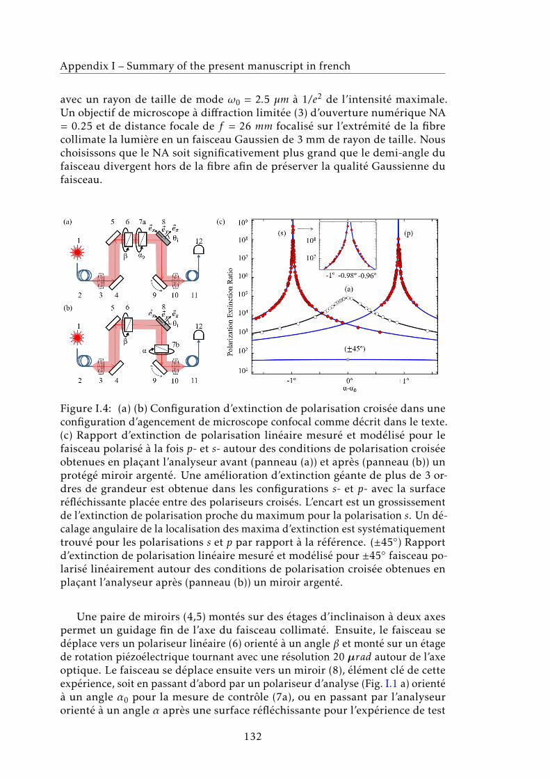
Appendix I – Summary of the present manuscript in french
avec un rayon de taille de mode ω0 = 2.5 µm à 1/e2 de l’intensité maximale.Un objectif de microscope à diffraction limitée (3) d’ouverture numérique NA= 0.25 et de distance focale de f = 26 mm focalisé sur l’extrémité de la fibrecollimate la lumière en un faisceau Gaussien de 3 mm de rayon de taille. Nouschoisissons que le NA soit significativement plus grand que le demi-angle dufaisceau divergent hors de la fibre afin de préserver la qualité Gaussienne dufaisceau.
Figure I.4: (a) (b) Configuration d’extinction de polarisation croisée dans uneconfiguration d’agencement de microscope confocal comme décrit dans le texte.(c) Rapport d’extinction de polarisation linéaire mesuré et modélisé pour lefaisceau polarisé à la fois p- et s- autour des conditions de polarisation croiséeobtenues en plaçant l’analyseur avant (panneau (a)) et après (panneau (b)) unprotégé miroir argenté. Une amélioration d’extinction géante de plus de 3 or-dres de grandeur est obtenue dans les configurations s- et p- avec la surfaceréfléchissante placée entre des polariseurs croisés. L’encart est un grossissementde l’extinction de polarisation proche du maximum pour la polarisation s. Un dé-calage angulaire de la localisation des maxima d’extinction est systématiquementtrouvé pour les polarisations s et p par rapport à la référence. (±45◦) Rapportd’extinction de polarisation linéaire mesuré et modélisé pour ±45◦ faisceau po-larisé linéairement autour des conditions de polarisation croisée obtenues enplaçant l’analyseur après (panneau (b)) un miroir argenté.
Une paire de miroirs (4,5) montés sur des étages d’inclinaison à deux axespermet un guidage fin de l’axe du faisceau collimaté. Ensuite, le faisceau sedéplace vers un polariseur linéaire (6) orienté à un angle β et monté sur un étagede rotation piézoélectrique tournant avec une résolution 20 µrad autour de l’axeoptique. Le faisceau se déplace ensuite vers un miroir (8), élément clé de cetteexpérience, soit en passant d’abord par un polariseur d’analyse (Fig. I.1 a) orientéà un angle α0 pour la mesure de contrôle (7a), ou en passant par l’analyseurorienté à un angle α après une surface réfléchissante pour l’expérience de test
132

Appendix I – Summary of the present manuscript in french
(7b). Nous avons également monté l’analyseur sur un étage de rotation pié-zoélectrique. Le miroir (9) monté sur un étage piézoélectrique à deux axes quipermet d’orienter le faisceau dans un objectif de microscope (10) identique à(3) focalisant la lumière dans le coeur d’une fibre monomode (11) identique à(2) permettant le filtrage confocal modal et la détection optique (12) à l’autreextrémité du câble fibre de 5 m.
Cet arrangement confocal simule les composants essentiels d’un microscopeconfocal à fluorescence résonnante. Le plan de surface réfléchissant (8) à 45◦
d’incidence, définit l’état de polarisation standard p et s avec des projections lelong de ~ex et ~ey respectivement. Les surfaces de test réfléchissantes en position (8)de la Fig. I.4a,b que nous avons utilisé dans ce travail sont des mirroirs commer-ciaux en argent protégé, aluminium, or évaporé, diélectrique, de Bragg à hauteréflexion ainsi que les cubes séparateurs non polarisants. Toutes ces surfacesréfléchissantes sont généralement utilisées dans des microscopes confocaux àdiffraction limitée. Les résultats étaient qualitativement très similaires pourtoutes ces surfaces réfléchissantes. Nous choisissons de montrer ici les donnéesmesurées avec des miroirs en argent uniquement, ceci à l’exception des donnéesmesurées à des fins de comparaison sur une surface de verre réfléchissant del’air (comme discuté au chapitre 4).
Nous discutons maintenant des mesures dans la configuration illustrée dansla figure I.4b, pour laquelle la surface de test réfléchissante est comprise entre lepolariseur et l’analyseur. Tout d’abord, l’angle du polariseur β est ajusté prèsde 0 ou π/2, respectivement pour p ou s polarisation, tout en définissant l’anglede l’analyseur α près de la polarisation croisée à β ±π/2. Ensuite, le polariseuret l’analyseur sont tournés finement pour atteindre l’extinction maximale auxvaleurs β et α respectivement. Une fois l’optimisation est atteinte, β reste intacteet l’analyseur dans son rotateur est ensuite placé avant la surface réfléchissantejuste après le polariseur pour notre mesure d’extinction de contrôle (Fig.I.4a).L’angle de l’analyseur doit alors être ajusté à une nouvelle valeur α0 afin derécupérer l’extinction nominale maximale inhérente aux polariseurs; α0 définitalors la référence p ou s. Les valeurs d’extinction mesurées en fonction de l’anglede l’analyseur α en référence à α0 sont représentées sur la Fig. I.4c pour lamesure de contrôle (Fig. I.4a) ainsi que pour les polarisations p et s dans laconfiguration (Fig. I.4b). Deux observations frappantes ressortent. (i) Pour tousles réflecteurs testés indiqués ci-dessus, le rapport d’extinction obtenu de cettemanière a été amélioré au-delà de 108 lorsque le miroir de test est compris entrele polariseur et l’analyseur, réduisant ainsi considérablement la fuite de polari-sation des polariseurs. (ii) L’angle de l’analyseur pour l’extinction maximale estdécalé de α0 de +0.898◦ et −0.977◦ respectivement pour les polarisations p ets, un écart angulaire significatif étant donné notre résolution d’environ 10 −3
deg. Dans le chapitre I.3, nous présentons une première explication de ces deuxobservations frappantes.
133

Appendix I – Summary of the present manuscript in french
I.3 Chapitre 3: Les origines physiques de l’annulationde fuite de polarisation
Intuitivement, la réduction significative du champ de fuite de polarisation doittrouver son origine dans un effet d’interférence destructeur. Le premier défipour trouver une réponse à notre problème est de proposer un modèle de fuitede polarisation. En effet, de nombreuses facteurs entraînent des fuites de po-larisation telles que la diffusion de la lumière, le désalignement, et des erreurslors du processus de fabrication des polariseurs croisés. L’hypothèse que nousfaisons sur l’origine physique de la fuite de polarisation est qu’elle est due à unediffusion cohérente sans perte telle que les inclusions de diffusion de Rayleighdans le cristal. En particulier, lorsque la lumière traverse une feuille polarisanteconstituée de chaînes de nanoparticules, elle interagit avec le milieu et celaprovoque la diffusion de la lumière. Les photons avec une direction de polarisa-tion le long des chaînes sont fortement absorbés, alors que l’absorption est faiblepour les photons avec une direction de polarisation perpendiculaire à ceux-ci.L’absorption fait vibrer les nanoparticules qui réémettent des photons dans desdirections aléatoires, mais avec la même fréquence et la même longueur d’onde.La diffusion de Rayleigh est un type d’interaction de diffusion cohérente qui faitque la lumière transmise est (π/2) déphasée avec le faisceau lumineux initial.Dans cette interaction, l’énergie des particules diffusantes n’est pas modifiée.et la fuite doit être invariante sur une rotation angulaire arbitraire autour del’axe optique. Dans notre cas la fuite nominale mesurée est (1.5 ± 0.5) × 105
(voir Fig. I.4c). On note que notre formalisme peut également être étendu auxpolariseurs circulaires.
Après un long mais simple calcul (équation (3.6), Annexe A.3), nous déter-minons l’intensité lumineuse juste après l’analyseur. Parce que la surfaceréfléchissante a des composantes réelles et imaginaires des coefficients de Fres-nel, on montre que pour une ” valeur suffisamment petite ” de fuite on peuttoujours trouver un choix des angles α,β qui conduit à une annulation parfaitede la fuite indésirable. Ceci est toujours vrai dans des conditions de réflexioninterne totale ce qui est le cas d’un miroir métallique dans le domaine visibleet infrarouge et pour un cube séparateur de faisceau typique. Une «valeur suff-isamment petite» de dépolarisation pour obtenir une annulation parfaite signifiedans le cadre de notre travail typiquement < 6×10⁻³ lors de l’utilisation d’unmiroir argenté comme nous nous l’avons dérivés dans le texte. La surface detest réfléchissante en combinaison avec la rotation des polariseurs agit pourinterférer de manière destructive avec la fuite de polarisation sans perte invari-ante de rotation résiduelle inhérente même aux meilleurs polariseurs linéairescommerciaux. Inversement, pour une surface purement diélectrique un tel verre(c’est-à-dire BK7) réfléchissant du côté air, pour lequel les coefificents de Fresnelpour p et s sont tous deux réels, aucune annulation de fuite de polarisationcomplète n’était possible.
Pour avoir une meilleure idée des paramètres pertinents en pratique pourl’annulation presque parfaite de la fuite de polarisation, nous illustrons lesmesures complètes et le modèle dans la Fig. I.4 qui sont obtenues en utilisant
134

Appendix I – Summary of the present manuscript in french
l’équation (3.6) et en tenant compte de manière convaincante de l’amplificationd’extinction de polarisation croisée et du léger décalage de rotation du polariseuret de l’analyseur nécessaire pour l’atteindre. Pour un miroir argenté parfait etune fuite de polarisation de 105 on évalue un taux de chromaticité de 0.0019◦/nmpour une longueur d’onde autour de λ = 905 nm . Dans cet exemple particulier,en gardant l’angle de l’analyseur à la valeur d’extinction maximale de 905 nm,la longueur d’onde pourrait être décalée jusqu’à ±10 nm tout en maintenantl’extinction à un niveau > 107.
À ce stade, nous avons pu conclure notre travail ici car nous avons pu ex-pliquer de manière convaincante toutes les caractéristiques de l’extinction depolarisation renforcée. Notre analyse a cependant occulté jusqu’à présent unpoint crucial, à savoir le fait expérimental que l’annulation de fuite n’étaitmesurable que dans un agencement confocal, point qui sera élucidé dans leschapitres suivants. Plus précisément, l’analyse que nous avons menée conduisantau résultat principal dans l’équation (3.6) jusqu’à présent a été faite uniquementpour une onde plane pour laquelle le formalisme de la matrice de Jones estvalide. En réalité cependant, la taille finie du faisceau laser Gaussien collimatéimpose une distribution d’onde angulaire finie autour de l’angle d’incidencesur le miroir [29]. Les coefficients de Fresnel pour p et s deviennent alors unefonction de la distribution angulaire [29]. Ceci, comme nous le verrons, conduità des effets de dépolarisation géométriques importants sous forme de nouveauxmodes optiques limitant l’extinction totale à la plage 104. Nous verrons qu’unedisposition confocale filtre les modes de dépolarisation et que le résultat de cechapitre se révèle fortuitement exploitable.
I.4 Chapitre 4: Transformation modale de la réflec-tivité d’un faisceau Gaussien polarisé
Pour expliquer l’origine du rapport de réjection de polarisation étonnammentélevé > 108, nous avons effectué une imagerie par balayage x,y de l’intensitédétectée dans des conditions de polarisation croisée. L’imagerie peut être réaliséeen balayant un miroir (9) ou en balayant la position spatiale de la fibre collec-trice dans le plan focal de l’objectif de focalisation (Fig. I.4b). Dans l’absence desurface réfléchissante entre l’analyseur et le polariseur en polarisation croisée,à savoir la configuration de référence de la Fig. I.4a, les mesures de la Fig. I.5a,b (rangée du haut) montrent un mode pur TEM00 Gaussien champ atténué de8.3× 104 et 9.6× 10⁴ pour p et s faisceau polarisé, respectivement. Ce niveau estattendu pour les spécifications de fuite du polariseur. En revanche, lorsque nousplaçons l’analyseur après la surface de test réfléchissante, les mesures montrentque le mode se divise en deux lobes répartis le long de ~ey et situés au-dessuset au-dessous du plan de réflectivité. Dans cette configuration à polarisationcroisée, on trouve un «trou» d’intensité à l’emplacement du centre de la fibreoptique. Là, l’extinction d’intensité est légèrement supérieure à 108, un facteur100 de notre limite de détection de configuration réelle.
135
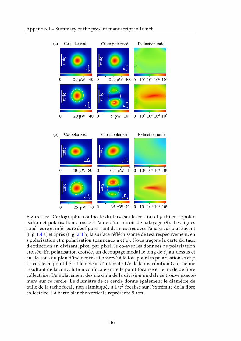
Appendix I – Summary of the present manuscript in french
Figure I.5: Cartographie confocale du faisceau laser s (a) et p (b) en copolar-isation et polarisation croisée à l’aide d’un miroir de balayage (9). Les lignessupérieure et inférieure des figures sont des mesures avec l’analyseur placé avant(Fig. I.4 a) et après (Fig. 2.3 b) la surface réfléchissante de test respectivement, ens polarisation et p polarisation (panneaux a et b). Nous traçons la carte du tauxd’extinction en divisant, pixel par pixel, le co-avec les données de polarisationcroisée. En polarisation croisée, un découpage modal le long de ~ey au-dessus etau-dessous du plan d’incidence est observé à la fois pour les polarisations s et p.Le cercle en pointillé est le niveau d’intensité 1/e de la distribution Gaussiennerésultant de la convolution confocale entre le point focalisé et le mode de fibrecollectrice. L’emplacement des maxima de la division modale se trouve exacte-ment sur ce cercle. Le diamètre de ce cercle donne également le diamètre detaille de la tache focale non alambiquée à 1/e2 focalisé sur l’extrémité de la fibrecollectrice. La barre blanche verticale représente 5 µm.
136

Appendix I – Summary of the present manuscript in french
Pour avoir une idée de la transformation modale mesurée pour p et s, nousavons mesuré et montré sur les Fig. I.6 et Fig. I.7 l’évolution de la lumière confo-cale cartes d’intensité pour différents angles de rotation de l’analyseur variationδα autour du mode divisé symétriquement. Fig. I.6d et I.7d montrent quantita-tivement pour les polarisations p et s les positions mesurées des décalages depics de faisceaux le long de ~ey et la division au-dessus et sous le plan d’incidenceen fonction de δα. Nous avons observé un comportement très similaire pour lescubes séparateurs de faisceaux généralement utilisés dans la configuration defluorescence résonnante, comme dans la référence [8, 9, 16, 18], à la différencecependant que ce chiffre équivalent semble plutôt reflété par rapport à l’axe∆y = 0. Dans tous les cas, une telle distribution d’intensité à lobes séparésrappelle beaucoup un mode TEM01 Hermite-Gaussien.
Les figures I.6c et I.7c montrent après une inspection minutieuse que lesminima d’intensité ou maxima d’extinction ne se produisent pas exactement ày = 0 mais sont plutôt très légèrement décalés symétriquement le long de y pourles deux la polarisation p et s. Cela signifie qu’il n’y a pas une seule position del’emplacement de fibre y qui puisse conduire à une extinction maximale pour lespolarisations p et s en même temps. Ceci est également clairement visible sur lafigure I.4c pour laquelle l’extinction est au-delà de 109 pour la polarisation s et108 pour p dans cette mesure particulière. Cette observation suggère clairementque les nouveaux modes le long de y semblent contribuer à stimuler l’extinctionbien au-delà du niveau de 108. Nous avons atteint un niveau record de 1010
pour lequel le facteur limitant était le bruit sombre de notre détecteur. Le défidans une telle expérience est d’avoir un rotateur de polarisation qui permet unpas avec des angles de rotation suffisamment petits. À ce stade, nous devonsdécouvrir pourquoi (i) la disposition confocale permet l’amélioration dramatiquede l’extinction comme le montre la Fig. I.4c, et (ii) pourquoi le faisceau se déplaceet se sépare en polarisation croisée en Fig. I.5(rangée du bas) et ceci toujoursau-dessus et au-dessous du plan d’incidence.
Pour répondre à ces questions, nous avons d’abord modéliser la distribu-tion spatiale du champ au plan focal de la lentille de focalisation juste avantla fibre optique monomode collectrice, puis utiliser la fibre collectrice commefonction de filtre Gaussien confocal portant la lumière vers le détecteur. Dansl’approximation paraxiale, la lentille de focalisation transforme chaque champd’onde plane de la distribution angulaire en une densité de champ dans la fo-cale plan, donc le faisceau atteignant le plan focal à la distance f résulte d’unesuperposition cohérente de toutes ces composantes focalisées (Annexe B.2). Untel problème a été modélisé pour une distribution de champ Gaussien dans [31]par Aiello et Woerdman. Nous en tirons ici une version simplifiée décrivant demanière pratique la physique essentielle nécessaire pour modéliser nos observa-tions. Lorsque le faisceau se réfléchit sur la surface de test, chaque composanted’onde plane acquiert un coefficient de réflexion de Fresnel. Nous montrons quela matrice de réflectivité de Jones transforme un mode Gaussien parfait incident,tel que l’équation (4.2), en la somme de TEM00, TEM01 et TEM10 Hermite-Gauss
137

Appendix I – Summary of the present manuscript in french
Figure I.6: Faisceau Gaussien p polarisé réfléchi par un miroir argenté. Évolutionmesurée (a) et simulée (b) de la cartographie d’imagerie confocale modale parextinction maximale (c) pour différents angles d’analyseur δα comme expliquédans le texte. En (d), les positions de décalage de crête et de division du faisceausont indiquées en unités de taille de faisceau ωf que nous avons modélisé pournotre miroir argenté ∆ = 102.48◦ et une fuite de 1/b2 = 8.3× 10⁴
Figure I.7: Faisceau Gaussien s polarisé réfléchi par un miroir argenté. Évolutionmesurée (a) et simulée (b) de la cartographie d’imagerie confocale modale parextinction maximale (c) pour différents angles d’analyseur δα comme expliquédans le texte. En (d), les positions de décalage de crête et de division du faisceausont indiquées en unités de taille de faisceau ωf que nous avons modélisé pourun miroir argenté ∆ = 100.7◦ et une fuite de 1 / b2 = 9.6× 10⁴
modes. Les indices pour TEM nm indiquent respectivement le nombre de nœuds.Le premier terme est la réflectivité normale de la surface de test que nous avonsutilisée dans la première partie de cet article. Le second terme est responsablede la génération d’un mode TEM10 le long du plan d’incidence. Ce terme est
138

Appendix I – Summary of the present manuscript in french
en fait responsable de l’effet Goos-Hänchen [32], car il a son origine physiquedans la dispersion angulaire des termes de réflectivité à θi . Ici les différentesondes planes les composants acquièrent des phases légèrement différentes lorsdu déplacement du faisceau dans le plan d’incidence. Comme cette matrice estdiagonale, l’effet Goos-Hänchen fait ne contribue pas à la dépolarisation dansle cas d’une polarisation p ou s parfaite. Le troisième terme, le plus pertinentpour ce travail, est chargé de générer un mode TEM01 hors plan d’incidenceavec deux lobes le long de l’axe y. Ce terme est la physique responsable del’effet Imbert-Fedorov [19,20,22,38] connu pour dévier un faisceau lumineuxréfléchi au-dessus ou au-dessous du plan d’incidence en fonction de son hélicitéde polarisation à droite ou à gauche. Notre calcul détaillé dans ce travail montreque ce terme provient purement de projections géométriques dans lesquellesle déphasage progressif gagné par chaque composante d’onde plane lors de laréflexion, se résume à une matrice diagonale croisée qui mélange les phases pet s composantes d’onde plane réfléchies décalées. Par conséquent, ce terme estresponsable d’une dépolarisation induite par réflectivité intrinsèque pour p et spolarisation même en utilisant des polariseurs idéalement parfaits. En raisonde la nature de projections purement géométriques de l’argumentation, le lienentre l’effet Imbert-Fedorov, la phase de Berry et l’effet spin-Hall de la lumièreest discuté dans la littérature [22, 38]. Nous pouvons voir à présent à partird’un argument de symétrie que notre arrangement confocal améliore l’extinctionde la polarisation croisée. Sans l’arrangement confocal, l’extinction aurait éténaturellement limitée dans la gamme 104 dans notre expérience comme nous leverrons après dans le texte.
Par ailleurs, nous avons exprimés la distribution de champ transmise par lepolariseur, le miroir et l’analyseur à l’ouverture arrière de la lentille de focali-sation en utilisant la transformée de Fourier (4.6). Après quelques calculationsalgèbriques (Annexe B.2), nous obtenons le champ de polarisation croisée pourla lumière incidente p (s). Un résultat important se dégage, à savoir que l’objectifamplifie considérablement le champ du mode Imbert-Fedorov. Il est facile demontrer que le facteur d’amplification de l’intensité lumineuse est ω2
0/ω2f . Dans
notre cas, nous obtenons une amplification de 3mm/2.5µm = 1200. C’est laraison pour laquelle nous pouvons détecter ce mode si clairement dans une con-figuration confocale. L’autre paramètre physique essentiel qui régit l’intensitédu champ du mode Imbert-Fedorov est la somme rp + rs donnée par le matériaureflétant les propriétés. Nous concluons que la cartographie des champs de modeImbert-Fedorov dans une configuration de microcopie confocale fournit un accèsdirect et sensible à l’amplitude et aux phases de réflectivité différentielle d’unesurface réfléchissante.
Ce résultat se révèle être dans un contexte différent dans le travail perspicaceet pionnier d’Aiello et al. [39]. Dans leur travail, les auteurs ont fourni dans uneapproximation paraxiale, une solution analytique complète pour la distributionde champ d’un faisceau Gaussien monomode réfléchi par un miroir. Le résultatessentiel de notre travail est que l’arrangement confocal transforme la taille du
139

Appendix I – Summary of the present manuscript in french
faisceau collimaté ω0 et la longueur de Rayleigh l et de la distribution du champAiello et al. [39] au plan miroir, en lf et ωf dans notre cas. Ce résultat semblebénin au début, mais comme évoqué plus haut, il s’agit d’une amplificationimportante de l’intensité du mode faible proportionnellement à ω2
0/ω2f . Aiello et
al. [39] a montré que c’est la taille finie du faisceau à la surface réfléchissantequi est responsable des termes de champ supplémentaires qui affectent le modeGaussien initial. De nos travaux, il devient maintenant clair ici qu’en utilisantun arrangement confocal, la taille du faisceau au niveau du miroir n’est paspertinente pour nos mesures mais plutôt la taille du faisceau focalisé qui joue unrôle crucial. Ce fait, au départ non intuitif, fournit un avantage précieux pourexplorer expérimentalement la géométrie de polarisation croisée avec une sensi-bilité suffisante et une résolution spatiale très fine. En particulier, l’extinction depolarisation croisée à extinction élevée est apparentée à la «procédure de mesurefaible» d’Aharonov et al. [40,41] que nous étendons ici à un agencement confocalpermettant l’avantage supplémentaire de la résolution spatiale. La littératurerécente [22] fournit une interprétation de la dépolarisation comme résultantd’une interaction spin-orbite efficace de la lumière se produisant à la surface dumiroir se manifestant sous la forme d’un effet spin-Hall de la lumière [42]. Dansle travail, nous nous limitons à une interprétation purement modale et laissonsde côté la discussion concernant le spin-orbite.
Le dernier point que nous avons aussi aborder pour obtenir une interpréta-tion quantitative complète de notre expérience est de traiter l’effet de la fonctionde filtre confocal de la fibre collectrice. La fibre monomode collecte et acheminele champ vers le photo-détecteur, elle le fait cependant en agissant comme unfiltre spatial Gaussien. Pour notre configuration symétrique illustrée à la Fig. I.4,nous éclairons et collectons la lumière avec des fibres monomodes de taille demode identique et avec des lentilles de collimation et de focalisation identiques.Le filtrage spatial est une convolution entre la distribution spatiale du champ auplan focal et le mode Gaussien de la fibre équivalant à une intensité de champdétectée par rapport à l’axe optique. Les résultats du calcul pour le champ sontles suivants (Annexe C.1). Nous obtenons d’abord la cartographie du champde référence sans utiliser de polariseur ni de surface réfléchissante vue par ledétecteur. Nous notons que la taille du faisceau au foyer semble maintenantêtre élargie d’un facteur
√2 en comparaison avec la distribution de l’équation
(4.7). Deuxièmement, nous avons trouvé que le filtrage confocal par convolu-tion avec un mode Gaussien conduit à une matrice de Jones efficace modifiéepour la surface réfléchissante agissant sur le champ vu depuis le détecteur (voirAnnexe C.2). Avec le filtrage confocal, les termes des champs Goos-Hänchenet Imbert-Fedorov (c’est-à-dire les deuxième et troisième termes des rhs dansl’équation) sont divisés par deux par rapport à l’équation (4.6) la matrice deJones liée aux polariseurs et à la fuite de polarisation reste inchangée. Avec cettedernière correction, nous avons maintenant toutes les équations nécessaires poursimuler la transformation modale induite par une surface réfléchissante agissantsur un faisceau Gaussien polarisé et ce pour tout arbitraire polarisation et niveaude fuite de polarisation. Le premier résultat important que nous obtenons de
140

Appendix I – Summary of the present manuscript in french
cette analyse est lorsque l’emplacement du centre de la fibre et l’axe du pointfocal coïncident le résultat est le même que celui trouvé dans l’analyse simplifiéedes ondes planes du chapitre 3 et l’équation d’annulation de polarisation don-née dans l’équation (3.6) est fortuite. C’est le cas car la fonction de filtrage del’agencement confocal élimine les modes de dépolarisation supérieurs. Sans le fil-trage confocal (voir Annexe D), le champ dépolarisé collecté en imagerie à champlarge du point focalisé limiterait l’extinction à 1.56 ×10³ et 2.1× 10³ pour p ets polarisé faisceau respectivement. Cela démontre le rôle clé de l’arrangementconfocal pour l’extinction de polarisation géante atteinte dans les mesures defluorescence de résonance de pointe [8, 9, 16, 18].
Comme le montre la Fig. I.5, notre calcul numérique est en parfait accordavec nos mesures pour l’argent. Nous avons confirmé quantitativement ces ré-sultats pour les miroirs de Bragg et les cubes séparateurs de faisceaux. Fig. I.6 etFig. I.7 montrent l’évolution de la transformation de mode près de la conditionde polarisation croisée pour une surface métallique. Dans notre expérience,nous mesurons les maxima typiques des lobes dans la plage de 0.3 à 1.4 ×10⁻⁶.Pour une raison non encore élucidée, nos intensités maximales mesurées sontplus faibles que celles modélisées. Nous pensons qu’il nous manque encore unecompréhension quantitative complète de la manière dont la fibre réceptrice filtreles modes non Gaussiens. En effet la sensibilité de notre configuration auraitdû permettre de détecter les modes de termes supérieurs TEM11 qui ont unesymétrie xy. Ces modes proviennent de la taille finie du faisceau Gaussien lerendant naturellement divergent [43]. En fait, nous pouvons utiliser le formal-isme exact développé ci-dessus pour montrer que de tels termes proviennentégalement de projections géométriques autour de l’axe optique. Cette fois, laprojection n’implique aucune surface réfléchissante mais juste la divergencenaturelle du faisceau avant la lentille, conduisant à un déphasage progressifgagné par chaque composante d’onde plane ici encore dépolarisant naturelle-ment le faisceau (voir Annexe E). En utilisant ce résultat pour nos paramètresd’expérimentation, l’intensité du pic de mode devrait être de 3.8 ×10⁻⁷, unevaleur qui se situe bien dans notre plage de sensibilité. C’est un fait étonnantque nous n’ayons observé aucune trace de ce signal TEM11. Il n’y a aucun doutecependant que ce mode est présent tel que mesuré dans [43], c’est pourquoinous pensons que notre compréhension de la façon dont la fibre optique filtre lesignal n’est pas encore complète.
I.5 Chapitre 5: Base de polarisation circulaire: di-recte imagerie de l’effet Imbert-Fedorov avec lamicroscopie confocale
En utilisant les résultats des chapitres précédents, nous déplaçons maintenantnotre exploration vers un aspect plus fondamental de l’optique afin de testerla capacité prédictive du modèle et plus important encore la puissance expéri-mentale de la microscopie confocale à révéler des effets de polarisation très
141

Appendix I – Summary of the present manuscript in french
faibles. En particulier ici, nous voulons nous concentrer sur la façon dont lessurfaces réfléchissantes affectent la lumière polarisée de manière circulaire. Cequi est bien établi, c’est qu’un faisceau laser à polarisation circulaire est réfléchiavec un décalage spatial transversal au plan d’incidence. Ce décalage d’Imbert-Fedorov, également connu sous le nom d’ effet spin-Hall de la lumière, a étémesuré pour la première fois par C. Imbert [20] pour un faisceau laser de lu-mière polarisée circulairement dans un prisme de verre dans des conditionsde réflectivité interne totale (Fig. I.8 (a) (b)). En fonction de la chiralité de sapolarisation circulaire, la trajectoire d’un faisceau polarisé circulairement sedéplacera au-dessus ou au-dessous du plan d’incidence lorsqu’il est réfléchi surune surface. Ce décalage est dû au couplage spin-orbite de la lumière à chaqueréflexion [21, 38, 46, 47] et est normalement très petit, typiquement, plusieursordres de grandeur plus petit que la longueur d’onde du photon. Pour cetteraison, il a auparavant nécessité des schémas de détection complexes limitantles investigations expérimentales détaillées. Ici, nous rapportons une nouvelleméthode pour mesurer et cartographier le décalage Imbert-Fedorov du faisceaulaser Gaussien basé sur une technique de polarisation croisée en champ sombredans un arrangement confocal.
Il existe une quantité considérable de littérature [42, 48] sur la mesure dudécalage d’Imbert-Fedorov en utilisant l’état de polarisation linéaire de la lu-mière où le mode de faisceau réfléchi se divise en deux lobes situés au-dessuset au-dessous du plan de réflectivité, comme déjà discuté dans les chapitresprécédents. À notre avis, cette approche n’est pas pertinente pour le couplagespin-orbite de la lumière car la notion de spin photonique est généralement liéeà la polarisation circulaire. Parce que ce déplacement est perpendiculaire auplan de réflectivité, l’effet Imbert-Fedorov a été renommé en effet spin-Hall dela lumière par des auteurs comme Onoda et al. [38], Bliokh et al. [46,47], Aielloet al. [49]. Ils ont interprété l’interaction spin-orbite de la lumière en termesde phases géométriques et de conservation du moment angulaire total de lalumière, comme déjà prédit par Liberman et al. En 1992 dans un milieu inho-mogène [21]. Des preuves plus récentes de cet effet ont été montrées par Bliokhet al. En utilisant des réflexions multiples dans un verre cylindrique dans lequelle décalage spin-Hall s’accumule le long d’une trajectoire hélicoïdale (Fig. I.8(c)).Dans ce cas, la division du spin-hall est amplifiée par de multiples réflexionset devient perceptible à un nombre de tours plus élevé (Fig. I.8 (d)). Dans cecontexte, la rotation bien connue du plan de polarisation pour une trajectoiretorsadée est expliquée à partir de la phase de Berry et de l’effet optique Magnus.La première observation de ce phénomène en cas de réflexion métallique a étédémontrée dans [49] par Aiello et son équipe. Dans leur expérience (Fig. I.8(e)),ils ont mesuré directement le décalage d’une lumière polarisée circulairementau lieu de regarder la division d’une lumière polarisée linéairement. Le décalagedétecté est de l’ordre du nanomètre et n’est pas mesurable à un angle d’incidenceinférieur à 50◦ (Fig. I.8(f)).
Malgré les différentes approches (Fig. I.8) qui ont été développées pour
142

Appendix I – Summary of the present manuscript in french
Figure I.8: (a) Dispositif expérimental global pour mesurer le décalage d’Imbert-Fedorov dans l’état de polarisation circulaire. Un faisceau laser, avec linéairehorizontal polarisation, traverse une lame quart d’onde puis une lame demi-onde couvrant la moitié du faisceau; le faisceau résultant, qui éclaire l’objetrectiligne CAB, est ainsi polarisé circulairement avec des hélicités opposées surses deux moitiés. Cela produira l’effet de doublement différentiel que nousontfait allusion à. Après avoir éclairé l’objet rectiligne CAB, le faisceau entre dansl’un de nos deux prismes multiplicateurs, et l’image de CAB est finalementobservée. La haute luminosité du prisme P permet de projeter cette image surun écran. (b) Image d’un objet rectiligne affichant le décalage transversal d’unfaisceau polarisé de manière circulaire. Les états de polarisation circulaire desdeux moitiés du faisceau sont indiqués. (Voir [20] pour plus de détails). (c)Mesure directe du spin-Hall de la lumière dans un cylindre de verre dans lequelle décalage s’accumule le long d’une trajectoire hélicoïdale. (d) Le décalagerelatif entre les deux composantes de spin par rapport aux tours de l’hélice.(Voir [47] pour plus de détails). (e) Le montage optique pour mesurer le décalagedifférentiel de polarisation d’un faisceau réfléchi par un film d’or épais. (f)Décalage différentiel de polarisation mesuré entre σ−/σ+ lumière polarisée enfonction de l’angle d’incidence. (Voir [49] pour plus de détails).
143

Appendix I – Summary of the present manuscript in french
étudier l’effet spin-Hall de la lumière, ce phénomène n’a pas été directement ob-servé. Il n’a été mesuré que dans certaines situations très particulières telles quedes réflexions multiples et un schéma de mesure faible. Cela limite l’utilisationde cet effet comme moyen pour générer, manipuler et détecter des photons polar-isés en spin. La seule preuve à ce jour est une mesure d’un décalage différentielde polarisation soit en faisant varier l’angle d’incidence ou la position du dé-tecteur. L’incertitude associée à la mesure du décalage soulève de nombreusesquestions quant à l’utilité et à la recherche expérimentale de cet effet. Dans cetravail, nous visons à faire un pont mental entre tous ces travaux et à fournirune explication claire des origines fondamentales du couplage spin-orbite de lalumière aux interfaces optiques. Pour cela, nous présentons une description mé-canique de la trajectoire d’une onde plane à polarisation circulaire en fonction deson spin et de son moment angulaire orbital. Nous trouvons une formule simpledu décalage Imbert-Fedorov qui révèle l’effet Hall de la lumière dépendant dela polarisation précédemment discuté dans la littérature. La même expressionest dérivée en utilisant l’approche Maxwell complète qui est pertinente pourexpliquer les subtilités importantes des déphasages induits par les coefficientsde Fresnel lors de la réflexion. Nous avons mis en place une expérience simpleet hautement reproductible pour observer et mesurer directement le décalaged’Imbert-Fedorov pour un faisceau Gaussien à polarisation circulaire.
Figure I.9: Mesures en champ clair dans un arrangement confocal pour lesangles d’incidence θi = 44◦(a)(e),30◦(b)(f ),21◦(c)(g),13◦(d)(h) en utilisant σ+ etσ− polarisation circulaire. Les mesures démontrent qu’aucun décalage techniqueparasite n’affecte notre configuration expérimentale dans des configurations pourlesquelles aucun décalage mesurable n’est attendu. Seul le demi-faisceau est af-fiché pour chaque polarisation circulaire σ+ et σ−. Les profils d’intensité mesuréspour la polarisation σ+ (cercles rouges) et σ− (cercles blancs) sont indiqués dansla ligne inférieure.
D’après le calcul pour une onde plane, le décalage Imbert-Fedorov devraitévoluer en cotgθi , en d’autres termes, nous sommes obligés d’explorer la région
144

Appendix I – Summary of the present manuscript in french
des petits angles pour pouvoir mesurer de grandes valeurs de décalage . Ici,nous nous sommes intéressés à observer le décalage aux angles d’incidenceθi = 44◦,30◦,21◦,13◦. En pratique, nous avons mis en place quatre expéri-ences différentes en modifiant l’angle d’incidence θi . En particulier, le miroirde test est déplacé par rapport au faisceau lumineux incident pour changerl’angle entre le faisceau et le miroir de surface de test. Pour chaque réglaged’angle d’incidence θi , nous avons mesurés l’intensité lumineuse, pour σ+ etσ− polarisation circulaire, mesurée en champ clair et sombre (Fig. I.9), respec-tivement. Seul un demi-faisceau est affiché pour chaque polarisation circulairepour une meilleure illustration de l’observation directe du décalage d’Imbert-Fedorov. Dans tous les cas, le profil d’intensité en champ clair est essentielle-ment un faisceau gaussien TEM 00 pour la polarisation σ+ et σ−, respectivement.L’emplacement de l’intensité du pic est centré à 0, il n’y a pas de dérive parasitetechnique de position maximale du faisceau laser pendant le processus de bal-ayage confocal qui pourrait être causée par un mauvais montage mécanique despièces optomécaniques ou lors de la rotation de composants optiques tels que laquart d’onde. Ces mesures (Fig. I.9) ont pour but d’évaluer les performances depositionnement du faisceau de notre configuration et aussi la fidélité et la sta-bilité à long terme du décalage Imbert-Fedorov mesuré avec notre arrangementconfocal en champ sombre. Nous avons vérifié expérimentalement la stabilitéde la position des maxima du faisceau θi = 44◦,30◦,21◦,13◦ comme le montre laFig. I.9(e)(f)(g)(h) attestant de la robustesse du montage expérimental.
En nous appuyant sur notre modèle détaillé pour les faisceaux laser Gaussiensdérivé pour la première partie de ce travail, nous avons vérifié quantitative-ment que le décalage augmente de manière significative en diminuant l’angled’incidence, ceci, à notre connaissance, est un nouveau régime qui n’était pasexplorée précédemment. Le modèle analytique montre un excellent accordavec nos mesures effectuées sur un miroir en argent. En particulier, le modèlerévèle clairement un régime d’angle d’incidence plus faible en dessous duquell’approche simpliste de la quasi-onde plane conduirait à une divergence nonphysique du décalage aux angles de fuite. Dans un régime d’angles aussi bas,notre modèle élimine cette divergence de décalage et prédit à la place unetransformation modale des photons minoritaires réfléchis vers le mode Hermite-Gaussien supérieur suivant d’une manière très similaire à celle explorée dans lapremière partie de ce travail. Les premières données indiquent la transition versun tel régime.
En conclusion, nous avons présenté une nouvelle méthode pour mesureret cartographier le décalage Imbert-Fedorov basée sur une technique de po-larisation croisée en champ noir dans un arrangement confocal. Dans notreconfiguration de champ sombre proposée sous polarisation circulaire, la ma-jorité des photons réfléchis sur une surface qui ne contribuent pas au décalagesont filtrés. Les photons minoritaires possèdent la chiralité appropriée pour lecouplage spin-orbite de la lumière permettant ainsi le grossissement du décalageImbert-Fedorov de plusieurs ordres de grandeur. Nous avons vérifié que le
145

Appendix I – Summary of the present manuscript in french
Figure I.10: Décalage Imbert-fedorov mesuré pour une polarisation circulaireσ± en unité de rayon de taille du faisceau ωf dans le cas d’un miroir argenté etpour une longueur d’onde laser λ = 905nm. On trace la position des maximad’intensité pour une onde plane (trait en pointillé) et un faisceau gaussien (traitplein) réfléchi par un miroir d’argent en fonction de l’excitation et de la détectionde polarisation. σ± Dark-field et σ± Bright-field désignent le dark-field (σ±Mσ±)et le Bright-field (σ±Mσ∓) configurations respectivement, lorsque le miroir (M)est placé entre deux polariseurs circulaires. Les mesures à θi = 13◦ montrentclairement le départ de la divergence d’approximation de l’onde plane (trait enpointillé) pour de faibles angles d’incidence. Le modèle est en très bon accord(trait plein).
décalage hors plan d’incidence mesuré de cette manière est une conséquencedirecte de la conservation du moment cinétique total.
I.6 Chapitre 6: Conclusion et perspectives
Notre étude fournit une boîte à outils robuste pour une nouvelle façon de fairedes expériences de spectroscopie de fluorescence et de polarimétrie à l’aidede la microscopie confocale. Nous avons exposé une méthode expérimentalesystématique basée sur un agencement de microscopie confocale pour obtenirune amélioration géante de l’extinction de polarisation croisée en champ som-bre et ce jusqu’à 3 ordres de grandeur et éventuellement au-delà. Nous avonsconstaté que l’effet exploite les propriétés matérielles d’une surface ou d’uneinterface sous condition de réflectivité interne totale notamment. En termesplus généraux, l’effet s’est avéré être entièrement régi par la différence de phase,telle qu’induite par les cubes séparateurs de faisceaux et les miroirs de Bragg,entre la réflectivité des composantes lumineuses polarisées dans et hors du pland’incidence. Maintenant que le principe de base de l’annulation de la fuite depolarisation est établi, il existe des options pour améliorer la limite de détectionexpérimentale du rapport d’extinction de polarisation croisée. Tout d’abord,
146

Appendix I – Summary of the present manuscript in french
il est possible d’améliorer le rapport signal sur bruit. En général, il est utiled’augmenter la puissance d’entrée optique par un meilleur alignement. Cepen-dant, cela dépend principalement de l’application. Dans les mêmes cas, les lasersbruyants ne peuvent pas être stabilisés et un type et un modèle appropriés dephoto-détecteur peuvent (et ne peuvent pas) améliorer le rapport signal / bruit.La deuxième possibilité consiste à amplifier la précision de l’angle de rotation.Il est démontré au chapitre I.4 qu’une résolution de positionnement de 10−6
degrés permet de mesurer une valeur de rapport d’extinction au niveau de 1011
et au-delà. Il est pratiquement possible d’obtenir une résolution de rotationde sous-taille avec des contrôleurs d’attocube sélectionnés. Une solution déjàexistante est le rotateur à roulement ECR4040/Al/NUM/RT avec une ouvertureintégrée de 1/2", adapté aux expériences optiques. Il est conçu pour des condi-tions ambiantes avec une position angulaire fine de 0.04 m◦.
De plus, nous avons également présenté l’analyse modale théorique de laréflectivité du faisceau. En effet, la modélisation de cet effet nous a conduit àsimuler et cartographier dans les moindres détails la transformation de faisceauxGaussiens proches de la polarisation croisée en modes supérieurs d’Imbert-Fedorov, une physique régie essentiellement par la divergence finie d’un faisceauGaussien réfléchissant sur une surface. Jusqu’à présent, les résultats ont ététrès prometteurs jusqu’à la transformation du premier ordre en x et y. Uneapplication potentielle prometteuse de notre approche serait de simuler et decartographier la transformation de faisceaux Gaussiens à des modes d’ordresupérieur. Jusqu’à présent, nous n’avons observé aucune trace du signal de modeTEM11. Il n’y a aucun doute cependant que ce mode est présent tel que mesurédans [43], c’est pourquoi nous pensons que notre modèle n’est pas encore com-plet. Les travaux futurs devraient également se concentrer sur l’améliorationde la qualité du taux d’extinction dans un dispositif confocal du monde réelcomposé de plusieurs miroirs et cubes séparateurs de faisceaux de géométriesdifférentes et complexes. Nous sommes convaincus que notre modèle servirade base pour la mise en place de la pierre angulaire de tout futur système despectroscopie optique. Le présent modèle est basé sur une approche d’expansiond’onde plane de Maxwell pure. L’étape suivante consiste à inclure la connexionentre l’effet Imbert-Fedorov et les phases géométriques. Ceci est absolumentessentiel dans la conception et la conception de dispositifs optiques modernesbasés sur le spin.
Dans le chapitre I.5, nous avons présenté une observation directe du décalageImbert-Fedorov, c’est-à-dire l’effet spin-Hall pour le spin vers le haut et versle bas de la lumière (polarisation circulaire). Cela n’a jamais été clairement vudans un manuel. Nous avons démontré que l’Imbert-Fedorov, comme il est ditdans les manuels scolaires, que (i) un faisceau laser se déplace hors du pland’incidence spéculaire lorsque la lumière heurte une polarisation circulaire etest détectée dans la même polarisation circulaire. (ii) Le signe du décalage estdonné par la chiralité. Il s’agit d’une nouvelle découverte en microscopie et peutconduire à des problèmes de mesure ou à des opportunités pour le chercheur
147
Appendix 6 – Summary of the present manuscript in french
effectuant des mesures sous polarisation circulaire. Nous avons montré à lafois théoriquement et expérimentalement, que l’effet est une conséquence dela conservation du moment cinétique total entre le faisceau incident et réfléchi.Pour être convaincant, nous avons également vérifié la stabilité maximale de laposition du faisceau de notre installation. La situation idéalisée d’une lumièred’onde plane polarisée circulaire et d’un miroir parfait hautement réfléchissantest parfaitement prédictif, à savoir qu’il prédit un décalage de déplacementtypiquement dépendant de la co-tangente de l’angle d’incidence cotgθi . Ce beaurésultat est issu d’un calcul très simple qui considère le conservation du momentcinétique de la lumière projetée sur l’axe z perpendiculaire au miroir. Dans cetravail et dans des expériences de microscopie réelles, nous nous demandonscomment cela s’applique à un faisceau focalisé Gaussien dans une configurationconfocale. Pour répondre à cela, nous avons fait notre modèle calculs d’aborddans la limite de NA plus petit et ont trouvé exactement le même résultat pour ledécalage de l’emplacement du maximum de l’intensité du faisceau. Nous avonsdonc maintenant un régime pour lequel un mode Gaussien semble agit commeune onde plane. Nous vérifions notre théorie par des mesures expérimentalesà différents angles d’incidence. Notre approche expérimentale présente un cer-tain nombre de similitudes avec la technique de mesure faible, la principaledifférence est que nous mesurons à une condition de polarisation croisée exacte.Des recherches expérimentales supplémentaires sont nécessaires pour compren-dre l’origine de la faible amplification de la mesure du décalage déjà rapportédans la littérature [42, 48]. C’est une question importante pour les recherchesfutures.
Ce travail ouvre la voie à la conception méthodique de microscopes à fluo-rescence à résonance laser sensible avec une extinction de fond extrême, pourune large gamme d’applications en optique quantique et en physique du solide.Les nouvelles méthodes développées pour ce travail peuvent également être ap-pliquées pour mesurer les propriétés optiques des matériaux et les applicationsde polarimétrie.
148

Bibliography
[1] Benelajla, M., Kammann, E., Urbaszek, B. & Karrai, K. The physical originsof extreme cross-polarization extinction in confocal microscopy. arXiv:2004.13564 (2020). URL https://arxiv.org/abs/2004.13564.
[2] Aharonovich, I., Englund, D. & Toth, M. Solid-state single-photon emitters.Nature Photonics 10, 631 (2016).
[3] Högele, A. et al. Dynamic nuclear spin polarization in the resonant laserexcitation of an InGaAs quantum dot. Physical Review Letters 108, 197403(2012).
[4] Paillard, M. et al. Spin relaxation quenching in semiconductor quantumdots. Physical Review Letters 86, 1634 (2001).
[5] Högele, A. et al. Voltage-controlled optics of a quantum dot. Physical ReviewLetters 93 (2004).
[6] Atatüre, M. et al. Quantum-dot spin-state preparation with near-unityfidelity. Science 312, 551–553 (2006).
[7] Gerardot, B. D. et al. Optical pumping of a single hole spin in a quantumdot. Nature 451 (2008).
[8] Vamivakas, A. N., Zhao, Y., Lu, C.-Y. & Atatüre, M. Spin-resolved quantum-dot resonance fluorescence. Nature Physics 5, 198–202 (2009).
[9] Kaldewey, T. et al. Far-field nanoscopy on a semiconductor quantum dot viaa rapid-adiabatic-passage-based switch. Nature Photonics 12, 68–72 (2018).
[10] Nguyen, H.-S. et al. Ultra-coherent single photon source. Applied PhysicsLetters 99, 261904 (2011).
[11] Najer, D. et al. A gated quantum dot strongly coupled to an optical micro-cavity. Nature 1–1 (2019).
[12] Kumar, S. et al. Resonant laser spectroscopy of localized excitons in mono-layer wse 2. Optica 3, 882–886 (2016).
[13] Nowak, A. et al. Deterministic and electrically tunable bright single-photonsource. Nature communications 5, 1–7 (2014).
149
Appendix 6 – BIBLIOGRAPHY
[14] Müller, M., Bounouar, S., Jöns, K. D., Glässl, M. & Michler, P. On-demandgeneration of indistinguishable polarization-entangled photon pairs. NaturePhotonics 8, 224 (2014).
[15] Schöll, E. et al. Resonance fluorescence of GaAs quantum dots with near-unity photon indistinguishability. Nano Letters 19, 2404–2410 (2019).
[16] Kuhlmann, A. V. et al. Charge noise and spin noise in a semiconductorquantum device. Nature Physics 9, 570–575 (2013).
[17] Ollivier, H. et al. Reproducibility of high-performance quantum dot single-photon sources. ACS Photonics 7, 1050–1059 (2020). URL https://doi.
org/10.1021/acsphotonics.9b01805.
[18] Kuhlmann, A. V. et al. A dark-field microscope for background-free detec-tion of resonance fluorescence from single semiconductor quantum dotsoperating in a set-and-forget mode. Review of scientific instruments 84,073905 (2013).
[19] Fedorov, F. I. K teorii polnogo otrazheniya. Doklady Akademii Nauk SSSR105, 465–468 (1955).
[20] Imbert, C. Calculation and experimental proof of the transverse shiftinduced by total internal reflection of a circularly polarized light beam.Physical Review D 5, 787 (1972).
[21] Liberman, V. S. & Zel’dovich, B. Y. Spin orbit interaction of a photon in aninhomogeneous medium. Physical Review A 46, 5199 (1992).
[22] Bliokh, K. Y., Rodríguez-Fortuño, F. J., Nori, F. & Zayats, A. V. Spin-orbitinteractions of light. Nature Photonics 9, 796 (2015).
[23] Ozawa, T. et al. Topological photonics. Rev. Mod. Phys. 91, 015006 (2019).
[24] Benelajla, M., Kammann, E., Urbaszek, B. & Karrai, K. Modal imaging ofa laser gaussian-beam reflected off a surface. Proceedings 11485 (114850E(2020)). URL https://doi.org/10.1117/12.2568365.
[25] Mollow, B. R. Power spectrum of light scattered by two-level systems.Physical Review Letters 188, 1969–75 (1969).
[26] Shree, S. et al. High optical quality of MoS2 monolayers grown by chemicalvapor deposition. 2D Materials 7 (2019).
[27] Stern, F. Elementary theory of the optical properties of solids. In Solid statephysics, vol. 15, 299–408 (Elsevier, 1963).
[28] Johnson, P. B. & Christy, R.-W. Optical constants of the noble metals.Physical review B 6, 4370 (1972).
[29] Novotny, L. & Hecht, B. Principles of nano-optics (Cambridge universitypress, 2012).
150

Appendix 6 – BIBLIOGRAPHY
[30] Goodman, J. Introduction to fourier optics (1968).
[31] Aiello, A. & Woerdman, H. The reflection of a maxwell-gaussian beam by aplanar surface. arXiv preprint arXiv:0710.1643 (2007).
[32] Goos, F. & Hänchen, H. Ein neuer und fundamentaler versuch zur totalre-flexion. Annalen der Physik 436, 333–346 (1947).
[33] Artmann, K. V. Berechnung der seitenversetzung des total-reflektiertenstrahles. Ann. Phys. Leipzig 2, 87–102 (1948).
[34] Tamir, T. Nonspecular phenomena in beam fields reflected by multilayeredmedia. J. Opt. Soc. Am. A 3, 558–565 (1986).
[35] Horovitz, B. R. & Tamir, T. Lateral displacement of a light beam at adielectric interface. J. Opt. Soc. Am. 61, 586–594 (1971).
[36] Ra, J. W., Bertoni, H. L. & Felsen, L. B. Reflection and transmission of beamsat a dielectric interface. SIAM J. Appl. Math. 24, 396–413 (1973).
[37] Nasalski, W. Longitudinal and transverse effects of nonspecular reflection.J. Opt. Soc. Am. A 13, 172–181 (1996).
[38] Onoda, M., Murakami, S. & Nagaosa, N. Hall effect of light. Physical ReviewLetters 93, 083901 (2004).
[39] Aiello, A. & Woerdman, J. Role of beam propagation in goos–hänchen andimbert–fedorov shifts. Optics letters 33, 1437–1439 (2008).
[40] Aharonov, Y., Albert, D. Z. & Vaidman, L. How the result of a measurementof a component of the spin of a spin-1/2 particle can turn out to be 100.Physical Review Letters 60, 1351 (1988).
[41] Duck, I., Stevenson, P. M. & Sudarshan, E. The sense in which a" weakmeasurement" of a spin-1/2 particle’s spin component yields a value 100.Physical Review D 40, 2112–2117 (1989).
[42] Hosten, O. & Kwiat, P. Observation of the spin hall effect of light via weakmeasurements. Science 319, 787–790 (2008).
[43] Erikson, W. L. & Singh, S. Polarization properties of maxwell-gaussian laserbeams. Phys. Rev. E 49, 5778–5786 (1994).
[44] Merano, M. et al. Observation of goos-hänchen shifts in metallic reflection.Physical Review Letters 15, 15928–15934 (2007).
[45] Karrai, K. & Miles, H. Inertial rotation device. Patent No: (Sep.6,2005). URL https://patentimages.storage.googleapis.com/a7/40/
8d/4a376e806e8773/US6940210.pdf.
151

Appendix 6 – BIBLIOGRAPHY
[46] Bliokh, K. Y. & Bliokh, Y. Conservation of angular momentum, transverseshift, and spin hall effect in reflection and refraction of an electromagneticwave packet. Phys. Rev. Lett. 96, 073903 (2006).
[47] Bliokh, K. Y., Niv, A., Kleiner, V. & Hasman, E. Geometrodynamics ofspinning light. Nature Photonics 2, 748–753 (2008).
[48] Ling, X. et al. Recent advances in the spin hall effect of light. IOP PublishingLtd 80 (2017).
[49] Hermosa, N., Nugrowati, A. M., Aiello, A. & Woerdman, J. Spin hall effectof light in metallic reflection. Optics letters 36, 3200–3202 (2011).
152