�����������������

Citation: Avram, F.; Adenane, R.;

Halanay, A. New Results and Open

Questions for SIR-PH Epidemic

Models with Linear Birth Rate, Loss

of Immunity, Vaccination and Disease

and Vaccination Fatalities. Symmetry

2022, 14, 995. https://doi.org/

10.3390/sym14050995

Academic Editors: Lorentz Jäntschi

and Sergei D. Odintsov

Received: 31 March 2022

Accepted: 7 May 2022

Published: 12 May 2022

Publisher’s Note: MDPI stays neutral

with regard to jurisdictional claims in

published maps and institutional affil-

iations.

Copyright: © 2022 by the authors.

Licensee MDPI, Basel, Switzerland.

This article is an open access article

distributed under the terms and

conditions of the Creative Commons

Attribution (CC BY) license (https://

creativecommons.org/licenses/by/

4.0/).

symmetryS S

Article

New Results and Open Questions for SIR-PH Epidemic Modelswith Linear Birth Rate, Loss of Immunity, Vaccination andDisease and Vaccination FatalitiesFlorin Avram 1,* , Rim Adenane 2 and Andrei Halanay 3

1 Laboratoire de Mathématiques Appliquées, Université de Pau, 64000 Pau, France2 Département des Mathématiques, Université Ibn-Tofail, Kenitra 14000, Morocco; rim.adenane@uit.ac.ma3 Department of Mathematics and Informatics, Polytechnic University of Bucharest,

062203 Bucharest, Romania; andrei.halanay@upb.ro* Correspondence: Florin.Avram@univ-Pau.fr

Abstract: Our paper presents three new classes of models: SIR-PH, SIR-PH-FA, and SIR-PH-IA, andstates two problems we would like to solve about them. Recall that deterministic mathematicalepidemiology has one basic general law, the “R0 alternative” of Van den Driessche and Watmough,which states that the local stability condition of the disease-free equilibrium may be expressed asR0 < 1, where R0 is the famous basic reproduction number, which also plays a major role in thetheory of branching processes. The literature suggests that it is impossible to find general lawsconcerning the endemic points. However, it is quite common that 1. When R0 > 1, there exists aunique fixed endemic point, and 2. the endemic point is locally stable whenR0 > 1. One would liketo establish these properties for a large class of realistic epidemic models (and we do not include hereepidemics without casualties). We have introduced recently a “simple” but broad class of “SIR-PHmodels” with varying populations, with the express purpose of establishing for these processes thetwo properties above. Since that seemed still hard, we have introduced a further class of “SIR-PH-FA”models, which may be interpreted as approximations for the SIR-PH models, and which includesimpler models typically studied in the literature (with constant population, without loss of immunity,etc.). For this class, the first “endemic law” above is “almost established”, as explicit formulas fora unique endemic point are available, independently of the number of infectious compartments,and it only remains to check its belonging to the invariant domain. This may yet turn out to bealways verified, but we have not been able to establish that. However, the second property, thesufficiency ofR0 > 1 for the local stability of an endemic point, remains open even for SIR-PH-FAmodels, despite the numerous particular cases in which it was checked to hold (via Routh–Hurwitztime-onerous computations, or Lyapunov functions). The goal of our paper is to draw attention tothe two open problems above, for the SIR-PH and SIR-PH-FA, and also for a second, more refined“intermediate approximation” SIR-PH-IA. We illustrate the current status-quo by presenting newresults on a generalization of the SAIRS epidemic model.

Keywords: epidemic models; varying population models; SIR-PH models; stability; next-generationmatrix approach; basic reproduction number; vaccination; loss of immunity; endemic equilibria;Routh–Hurwitz conditions

1. Introduction

Motivation. One of the hardest challenges facing epidemic models is dealing withmodels within which death is possible, in which the total population N varies, and inwhich the infection rates depend on N (as is the case in reality, except for a short period oftime at the start of an epidemic). As these features confront the researcher with challengingbehaviors (the first being that the uniqueness of the fixed endemic point may stop holding),sometimes hard to explain epidemiologically, it seems natural to attempt to identify the

Symmetry 2022, 14, 995. https://doi.org/10.3390/sym14050995 https://www.mdpi.com/journal/symmetry

Symmetry 2022, 14, 995 2 of 26

simplest class of realistic models for which a theory may be developed. The natural choiceis “standard incidence rates”—see (1), since models with nonlinear infection rates are quitecomplex—see for example [1–5] for the very complex dynamical behaviors which mayarise otherwise.

The next issue is choosing the type of birth function b(N) to work with. The easiestcase is when b(N) is constant, but this corresponds to immigration rather than birth, and soour favorite are linear birth rates b(N) = ΛN. A bonus for this choice, as well known, is thatnormalization by the total population leads to a model with constant parameters, whichlooks similar to classic constant population models, but involves some extra nonlinearterms—see (2). The well-studied classic models may then be recovered via a heuristic “firstapproximation” (FA) of ignoring the extra terms. This approximation, which deserves to beinvestigated rigorously via slow-fast/singular perturbation/homogenization techniques,has the merit of putting under one umbrella constant and varying population models withlinear birth rates.

At this point, let us mention that we believe that epidemic models should be ideallyparameterized by the two matrices F, V, which intervene in the next generation matrixapproach, which has been called disease-carrying and state evolution matrices [6,7]. Afoundational paper in this direction is [8], Arino shows that further simplifications arisefor models having only one susceptible class and disease-carrying matrix of rank one. Thefirst fundamental question, the uniqueness of the endemic point when R0 > 1, may beresolved explicitly for the “FA approximation” (and hence also for “small perturbations”,numerically). This has motivated us to propose [9,10] to develop the theory of this class ofmodels, which we call “Arino” or “SIR–PH” models.

Contributions and contents. The goal of our paper is to draw attention to two in-teresting open problems, for the SIR-PH, SIR-PH-FA, and also for a second, more refined“intermediate approximation” SIR-PH-IA. We illustrate the current status-quo by presentingnew results on a generalization of the SAIRS epidemic model of [11,12].

The SAIRS model (2) is presented in Section 2. The history of the problem and someoversights and errors in the literature are recalled in Section 2.1. The basic reproductionnumberR0 and the weakR0 alternative for the DFE equilibrium are established via thenext generation matrix approach in Section 2.2. The local stability of the endemic pointwhen the basic reproduction number satisfies R0 > 1 for the FA model is established inSection 2.3.

A review of the theory of SIR-PH models is provided in Section 3, and some newresults in Section 4.

The scaled SAIRS model is revisited in the Section 5, where some previous results inthe literature are corrected and completed.

2. The SAIRS Model with Linear Birth Rate

In this paper, we consider a ten parameters SAIR (also called SEIR in the classicliterature [13]) epidemic model inspired by [12,14–20], which we call SAIR/V+S (or SAIRfor short) as it groups together immunized people in an R/V compartment. The letterA (from asymptomatic) stands for the fact that the individuals in this compartment mayinfect the susceptibles. This important feature, already present in [13], was further studiedin [11,12,21]. The model studied in [12] is the most complete in the sense that it missesonly one of the parameters of interest, namely the important extra death rate due to thedisease—see for example [22]. The explanation for this omission in [12] lies probably in thefact that this paper follows the tradition of the “short term constant population epidemics”,in which the total population N is assumed constant, and the endemic point is uniqueand easy to find explicitly. Our paper investigates, for the model of [12], the topic of thefirst six papers cited, i.e., we attempt to deal with the variation of N(t) during epidemicsthat may last for a long time and which may never be totally eradicated. We generalizethe uniqueness of the endemic point and the local stability results of these six papers and,

Symmetry 2022, 14, 995 3 of 26

at the same time, draw attention to certain unnecessary assumptions and mistakes. Thehardest issue of global stability is only illustrated via some numerical simulations.

SAIR Model. Letting S(t), E(t), I(t), R(t), D(t) and De(t) represent Susceptibleindividuals, Exposed individuals, Infective individuals, Recovered individuals, naturallyDead individuals and Dead individuals due to the disease, respectively, the model weconsider is:

S′(t) = ΛN(t)− S(t)(

βiN(t)

I(t) +βe

N(t)E(t) + γs + µ

)+ γrR(t),

E′(t) = S(t)(

βiN(t)

I(t) +βe

N(t)E(t)

)− (γe + µ)E(t), γe = ei + er

I′(t) = eiE(t)− I(t)(γ + µ + δ), (1)

R′(t) = γsS(t) + erE(t) + γI(t)− (γr + µ)R(t),

D′(t) = µ(S(t) + E(t) + I(t) + R(t)) := µN(t),

D′e(t) = δI(t),

N(t) = S(t) + E(t) + I(t) + R(t) =⇒ N′(t) = (Λ− µ)N(t)− δI(t).

Epidemiologic meaning of the parameters:

1. Λ ∈ R≥0 and µ ∈ R≥0 denote the average birth and death rates in the population (inthe absence of the disease), respectively.

2. The parameters βi ∈ R≥0 and βe ∈ R≥0 denote the infection rates for infective andexposed individuals, respectively;

3. γs ∈ R≥0 is the vaccination rate, γe ∈ R≥0 is the rate at which the exposed individualsbecome infected or recovered, γr ∈ R≥0 denotes the rate at which immune individualslose immunity (this is the reciprocal of the expected duration of immunity), γ ∈ R>0is the rate at which infected individuals recover from the disease.

4. ei ∈ R≥0, er ∈ R≥0, are rates of transfer from E to I and R, respectively.5. δ ∈ R≥0 is the extra death rate in the infected compartment due to the disease.

Some particular cases.

1. If βe = er = 0, we obtain a SEIRS type model. If furthermore γr = γs = 0, we arrive tothe model masterly studied in [15]; if only one of these parameters is zero, we arriveto the models studied in [16–19].

2. If βi = γr = γs = 0 = δ, we obtain the SIQR model [23,24].

Remark 1. Note the notation scheme employed above, which could be applied to any compartmentalmodel. A linear rate of transfer from compartment m to compartment c is denoted by mc, and thetotal linear rate out of m is denoted by γm, which implies ∑c mc = γm, for example γe = ei + er.Extra death rates due to the epidemics in a department c are denoted by δc. An exception is madethough for the infectious compartment i, where we simply use the classic notations γ, δ, instead ofγi, δi. Our scheme would simplify a lot, if adopted, perusing the rather random notations used inthe literature.

The scaled model. It is convenient to reformulate (1) in terms of the normalizedfractions s = S

N , e = EN , i = I

N , r = RN . Using N′(t) = (Λ− µ)N(t)− δI(t), this yields the

following nine parameters SEIRS epidemic model (the common death rate µ simplifies,and an extra δi c appears in the equation of each compartment c–see for example [25] forsimilar computations).

s′(t) = Λ− s(t)(βii(t) + βe e(t) + γs + Λ) + γrr(t) + δs(t)i(t)(e′(t)i′(t)

)=

[s(t)

(βe βi

0 0

)+

(−(γe + Λ) 0

ei −(Λ + γ + δ)

)+ δit Id

](e(t)i(t)

)r′(t) = γss(t) + er e(t) + γi(t)− (γr + Λ)r(t) + δi(t)r(t)

. (2)

Symmetry 2022, 14, 995 4 of 26

Remark 2. Note that we have written the “infectious” middle equations to emphasize first thefactorized form, similar to that encountered for Lotka-Volterra networks—see for example [26].Secondly, for the factor appearing in these equations, we have emphasized the form

F−V + δiI2 := sB−V + δiI2. (3)

Note that the matrices F, V are featured in the famous the (Next Generation Matrix) approach [13],that some authors refer to them as “new infections” and “transmission matrices”, that [7] callthem the disease-carrying and state evolution matrices, and that ([27], Ch 5) gives a way to definean associated stochastic birth and death model associated to these matrices. The matrix B is fur-ther useful in defining and studying more general SIR-PH models—see [9,10] and below, and seealso [28], ([29], (2.1)), [6] for related works.

Since the computations will become soon very cumbersome, we will start using from now onthe following notations:

v0 = Λ + γr + γs,v1 = Λ + γe,v2 = Λ + γ + δ.

(4)

Note that vz, with z = {1, 2}, are the diagonal elements of V, and that v0 appears as denomi-nator in the DFE (9).

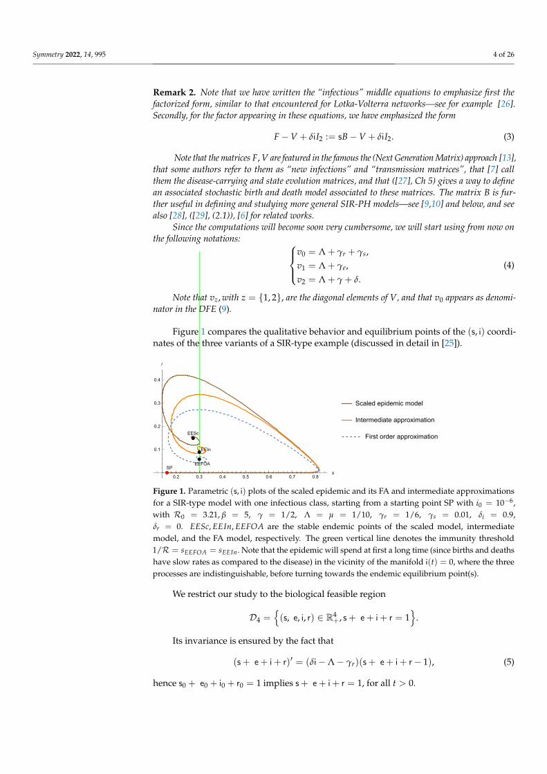
Figure 1 compares the qualitative behavior and equilibrium points of the (s, i) coordi-nates of the three variants of a SIR-type example (discussed in detail in [25]).

0.2 0.3 0.4 0.5 0.6 0.7 0.8s

0.1

0.2

0.3

0.4

i

SPEEFOA

EESc

EEIn

Scaled epidemic model

Intermediate approximation

First order approximation

Figure 1. Parametric (s, i) plots of the scaled epidemic and its FA and intermediate approximationsfor a SIR-type model with one infectious class, starting from a starting point SP with i0 = 10−6,with R0 = 3.21, β = 5, γ = 1/2, Λ = µ = 1/10, γr = 1/6, γs = 0.01, δi = 0.9,δr = 0. EESc, EEIn, EEFOA are the stable endemic points of the scaled model, intermediatemodel, and the FA model, respectively. The green vertical line denotes the immunity threshold1/R = sEEFOA = sEEIn. Note that the epidemic will spend at first a long time (since births and deathshave slow rates as compared to the disease) in the vicinity of the manifold i(t) = 0, where the threeprocesses are indistinguishable, before turning towards the endemic equilibrium point(s).

We restrict our study to the biological feasible region

D4 ={(s, e, i, r) ∈ R4

+, s+ e+ i+ r = 1}

.

Its invariance is ensured by the fact that

(s+ e+ i+ r)′ = (δi−Λ− γr)(s+ e+ i+ r− 1), (5)

hence s0 + e0 + i0 + r0 = 1 implies s+ e+ i+ r = 1, for all t > 0.

Symmetry 2022, 14, 995 5 of 26

We will work in three dimensions by eliminating r = 1− s− e− i. The first equationof (2) changes then, and the system becomes

s′(t) = Λ + γr − γr( e(t) + i(t))− s(t)[Λ + γr + γs + (βi − δ)i(t) + βe e(t)],(e′(t)i′(t)

)=

[(βes(t)− v1 βis(t)

ei −v2

)+ δi(t)I2

](e(t)i(t)

)(s, e, i) ∈ D3 := {(s, e, i) ∈ R3

+, s+ e+ i ≤ 1}

. (6)

Concerning fixed points, we note first, following ([15], (4.2)), ([17], (13)), the followingnecessary condition at a fixed endemic point:

s′ + e′ + i′ = 0⇔ e(γe − ei) + γi + sγs = γrr + Λr− δir

⇔ (1− (e + i + s))(Λ + γr − δi) = e(γe − ei) + γi + sγs =⇒ i < ic := min[1, (Λ + γr)/δ],(7)

where the last implications follows since the right hand side of the last equation in (7) ispositive, due to er = γe − ei ≥ 0.

Thus, the search for fixed points may be reduced to the domain

D f := D3 ∩ {i : i < ic = min[1, (Λ + γr)/δ]}. (8)

As a quick preview of the next generation matrix “factorization” idea, we note nowthat the disease free equation s′ = Λ − s(Λ + γs) + γr(1 − s) (defined by e = i = 0,r = 1− s) has fixed point

sd f e =Λ + γr

Λ + γr + γs=⇒ rd f e = 1− sd f e =

γs

Λ + γr + γs, (9)

whenever Λ+γr +γs 6= 0, which will be assumed from now on. Note this formula containsonly three of the parameters.

The other 6 parameters γ, δ, βi, βe, ei, γe intervene in the “infection equations” for e, i,and will determine the basic reproduction number (12)

R0 =sd f e

Λ + γe

[βe +

βieiΛ + γ + δ

]:= sd f eR,

whereR is precisely theR0 which would be obtained in the absence of vaccination.When δ = 0, our model (6) reduces to the eight parameters constant population model

studied in [12], which has a unique endemic point, with coordinates expressible in termsof R0; for example see =

sd f eR0

:= 1R . Its global stability is, however, hard to prove ([12],

Conjecture 15), and the authors resolve only the case βe < γ.

2.1. Some History of the SEIRS and SAIRS Varying Population Models

A first important paper on the varying population SEIRS model (recall that bothnotations SEIRS and SAIRS have been used already for the same model) is [14], whereβe = er = 0 and where a proportion q of vaccines is allocated to the newborn. We took forsimplicity q = 0, as this parameter does not modify in an essential way the mathematicsinvolved. Note that δ, Λ, γe, γs and γr are denoted in [14] by α, r, σ, p and ε, respectively.

Besides the typical weakR0 alternative, ([14], Thm 2.3(i)) establishes also global asymp-totic stability (GAS) of disease free equilibrium whenR0 < 1 and when either (I) βiγe

Λ+γe≤ δ,

(II) γs = 0, or a certain non-explicit condition holds. A second result ([14], Thm 2.3(ii))establishes the uniqueness of the endemic point whenR0 > 1, and , γr ≤ min[γe, γ].

Stimulated by the many open cases left above, in [15], the authors considered the particularcase βe = er = γr = γs = 0.As the authors explain, the difficulties met, especially in theglobal stability problem, forced them to devise new ingenious methods. (12) becomes nowR0 = βiγe

(γe+Λ)(Λ+γ+δ)(note that β, γe, Λ, δ and R0 are denoted in [15] by λ, ε, b, α and σ,

Symmetry 2022, 14, 995 6 of 26

respectively, and that sd f e = 1). Building on previous results in the limiting cases δ = 0 for SEIRmodels with constant population [30] and γe → ∞ for SIR models with varying populations [31],they establish the uniqueness and global stability of the endemic point ([15], Cor. 6.2, Thm6.5)whenR0 > 1.

Note that the Corollary is under the assumption of non-existence of non-constantperiodic solutions and the Theorem requires the additional assumption δ < γe; thus, thecomplementary case was left open.

Next, the reference [16] studied the case of waning immunity, leaving again open many cases.Note that the so-called “geometric approach to stability” method, initiated in [15,16,32], was usedmany times afterward —see for example [19].

Eleven years later, the authors in [17] re-attacked the [14] problem with βe = er =γr = 0 and vaccination γs ≥ 0 (denoted by aσ). We note, by adding the two infectionrates in ([17], Figure 1), which yields λ(1 − aσ), that the model depends only on aσ,and so introducing two parameters for γs unnecessarily complicates the mathematics.Furthermore, the infection rate λ(1− aσ) might as well be denoted by one parameter, andwe chose the classical β. Finally, one can relate their results to ours by substituting β withγ and setting σ = 1 (i.e., giving up the second source of infections), and λ = β/(1− γs).Then, ([17], (8))

R0 = sd f eβiγe

(Λ + γe)(Λ + γ + δ):= Rsd f e, (10)

whereR =

βiγe

(Λ + γe)(Λ + γ + δ)and sd f e =

ΛΛ + γs

.

See also (12).

Remark 3. Let us note two open problems left in [17].

1. ([17], Thm 2.1) proves the global stability of the DFE when

R ≤ 1

(by using the Lyapunov function γee + (γe + Λ)i, which is different from the Lyapunovfunction used in [33], e(γ + Λ + δ) + γei. This leaves open the caseR0 < 1 < R, when theDFE is locally, but perhaps not globally stable, and also the question of choosing the “mostperformant” Lyapunov function.

2. ([17], Thm 2.1) establishes global stability of a unique endemic point in certain cases andsuggests that outside those cases, “there may exist stable periodic solutions”.

Seven years later, the reference [18] revisited the [16] problem with γs = 0 and waningimmunity γr ≥ 0 (denoted by ρ). The authors remark that in this particular case, there arestill open questions: “We have not proved, but we strongly believe that ifR0 > 1, then thesystem (2) has one and only one endemic equilibrium and that this equilibrium is globallyasymptotically stable”. The [16] problem was revisited then in [19], who claims to havealso removed the restriction δ < γe of [15]; however, their crucial equation ([19], (3.28))is wrong, see Section 5. The fact that the papers [17,19] contain unnecessary conditions,mistakes, and wrong conjectures suggests that for complicated epidemic models withinfection rates depending on N, ingenuity stops being enough, and it must be accompaniedby verifications via symbolic software, rendered public, as is the case with our paper (inline with the so-called “reproducible research” [34]).

Finally, the authors in [12] apply the geometric approach to global stability, takinginto account vaccination and loss of immunity, and also the possibility that the exposed, orrather the asymptomatic, are infectious, but for a simplified constant population modelwith δ = 0, Λ ≥ 0. The basic reproduction number (12) becomes now ([12], (5))

R0 =

[βe +

βieiΛ + γ

]sd f e

γe + Λ

Symmetry 2022, 14, 995 7 of 26

(with the correspondence Λ→ µ, βe → βA, ei → α, er → δA, γ→ δI , γr → γ, γs → δ). Theglobal stability is proven only in the case βe < γ.

These multiple but only partially successful attempts at solving the [14] problemmotivated us to revisit it. (Yet another motivation was the literature on bifurcation analysisof SIR and SEIR-type models [1,3,5,35–37], and [2,20] which contains yet another plethoraof open problems.)

2.2. Warm-Up: The WeakR0 Alternative for the DFE Equilibrium

Note that the DFE (9) is a stable point for the disease-free equation

s′(t) = Λ + γr − s(t)(Λ + γr + γs).

Then, we may check that the quadratic—linear decomposition of(e′(t)i′(t)

)=

(βes(t) + δi(t)− (γe + Λ) βis(t)

ei δi(t)− v2

)(e(t)i(t)

)= F ( e, i)− V( e, i),

where

F ( e, i) =(

βes e+ βisi+ δ eiδi2

), V( e, i) =

((Λ + γe) e−ei e+ iv2

)satisfies the splitting assumptions of the NGM (Next Generation Matrix) method [13].

The partial derivatives at the DFE of F ( e, i),V( e, i) are

F = sd f e

(βe βi0 0

), V =

(v1 0−ei v2

), (11)

and

FV−1 =

(βesd f e βisd f e

0 0

)( 1v1

0ei

v1v21v2

)=

(sd f e

[βev1

+ βieiv1v2

]sd f e βi

v2

0 0

).

We may conclude then by the well-known next generation matrix result of [13] that:

Proposition 1. The SAIR/V+S basic reproductive number is

R0 := sd f eβt

v1v2, (12)

where vi were defined in (4) and where

βt := βiei + βev2. (13)

Furthermore, the weak R0 alternative (The strong R0 alternative [33] also covers he caseR0 = 1.) holds, i.e.,

1. IfR0 < 1⇔ (Λ+γr)βt < v0v1v2 then the disease-free equilibrium is locally asymptoticallystable.

2. IfR0 > 1⇔ (Λ + γr)βt > v0v1v2, the disease-free equilibrium is unstable.

Remark 4. The formula for R0 follows also from the [8] formula for SIR-PH models with newinfection matrix of rank one F = sα~β—see [9,10], and below, for the definition of this class. Thisformula becomes, after including demography parameters Λ,~δ,

R0 = ~β V−1α, V = −A + Diag(~δ + Λ~1),

Symmetry 2022, 14, 995 8 of 26

In the particular SAIRS case, this formula may be applied with the parameters defining themodel, which are

~β =(

βe, βi), α =

(10

), A =

(−γe 0

ei −γ

),~δ =

(0, δ

).

Finally, we will write

~a :=~1(−A) =(γe − ei, γ

)in this example,

for a quantity which will appear often below.—See for example (24) where we used the standardnotation in the theory of phase-type distributions.

A direct proof of Proposition (1) is also easy here. Indeed, after reducing (2) to a threeorder system by r = 1− s− e− i, the Jacobian matrix is

J =

−~βi + δi−Λ− γr − γs −sβe − γr s(δ− βi)− γr~βi sβe + iδ− v1 eδ + βis0 ei −γ + (2i− 1)δ−Λ

,

(where ~βi = βee + βii), and

JDFE =

−v0 −βesd f e − γr (δ− βi)sd f e − γr0 βesd f e − v1 βisd f e0 ei −v2

.

Note the evident block structure {s}, {e, i} (which is the driving idea behind the nextgeneration matrix method), with one negative eigenvalue −v0.

Now the “infectious” determinant v1v2 − sd f eβt is positive iff

v1v2(1− sd f eβt

v1v2) = v1v2(1−R0) > 0⇔ R0 < 1.

This is also the stability condition, since it may be shown that sd f eβt < v1v2 impliesalso the trace condition βesd f e − v1 − v2 < 0, and so theR0 alternative holds.

Remark 5. As usual, it is useful to introduce critical vaccination and critical “total contact” (recallβt = βiei + βev2) parameters, as the unique solutions of R0 = 1 with respect to γs and βt. Thecritical values are

γ∗s = (Λ + γr)

[βt

v1v2− 1]

:= (Λ + γr)[R− 1], β∗t =v0v1v2

Λ + γr=

v1v2

sd f e. (14)

These are particular cases of the SIR-PH Formulas (29).

2.3. The Endemic Point for the FA Approximation, and the Determinant Formula

We consider now the following “first approximation” (FA) of the SIR-PH-FA varyingpopulation dynamics

i′(t) = [s(t) B−V]i(t)s′(t) = Λ− s(t) ~βi(t)− (Λ + γs)s(t) + γrr(t)r′(t) =~ai(t) + s(t)γs − r(t)(γr + Λ)

(s(t), i(t), r(t)) ∈ R4+

, (15)

Symmetry 2022, 14, 995 9 of 26

where i(t) :=(

e(t)i(t)

),~β and ~a are defined in Remarks 4, and V in (11). Here the extra

deaths δ due to the disease in state i are kept, but the quadratic interaction terms involvingδi were neglected. Under this approximation, the endemic point and the determinant ofthe Jacobian have elegant formulas in terms of R0, some already discovered and othershidden in the particular cases of [11,12].

Remark 6. For this approximation, the sum of the variables is constant only if δ = 0; therefore, rmay not be eliminated, and we must work in four dimensions.

Lemma 1. (a) For the SAIR model (15) with extra deaths δ, put iee =

(eeeiee

)and

v0 := Λ + γr + γs,v1 := Λ + γe,v2 := Λ + γ + δ,v3 := (v1 + γr)v2 + γrei.

Then, the following formulas hold at the endemic point:

see =sd f e

R0= 1R ,(

eee

iee

)= Λ+γr

Λv3+γrδei(1− 1

R0)

(v2

ei

),

~βiee = βtΛ+γr

Λv3+γrδei(1− 1

R0) = Λ(R0−1)v0v1v2

Λv3+γrδei=: EI,

~aiee =Λ+γr

Λv3+γrδei(1− 1

R0) [γeγ + (Λ + δ)er],

ree =

(γs

(Λ + v2 + ei(Λ + δ)

)+ Λ(R− 1)(v2er + γei)

)× 1R(Λv3+γrδei)

.

(16)

(b) All the coordinates are positive iffR0 > 1.(c) The vector iee checks the general SIR-PH normalization Formula (36).

Proof. (a) One can do a direct computation or apply ([10], Prop. 2), a particular case ofwhich is included for completeness as Proposition 3, Section 3. That result is expressed interms of the Perron Frobenius eigenvector of the matrix M = 1

RB−V (for the 0 eigenvalue);

in our case, this is(

v2ei

), see second equation in (16).

(b) Is obvious.(c) May be easily checked, combining the last two rows in (16).

Remark 7. Several particular cases of this problem have been studied in the literature. The caseδ = 0 is studied in [12], and the reference [38] considered the case βe = γr = er = 0, δ > 0, where

α =

(10

), A =

(−γe 0γe −γ

),~at := (−A)t1 =

(0γ

),~β =

(0 βi

),~δ =

(0 δ

).

The normalization Formula (36) reduces in this case to

~βi = Λ

[R− 1

sd f e

]= Λ

(βiγe

(Λ + γ + δ)(γe + Λ)− 1)− γs.

Lemma 2. The following remarkable identity holds

Det(Jee) = Λv0v1v2(1−R0) = −Det(Jd f e), (17)

Symmetry 2022, 14, 995 10 of 26

where vi are defined in (4).

Proof. See the proof of Proposition 3.

Remark 8. We conjecture that the endemic point is always locally stable when 1 < R0. Wehave attempted to apply the classic Routh–Hurwitz–Lienard–Chipart–Schur–Cohn–Jury (RH)methods [39–41], which are formulated in terms of the coefficients of the characteristic polynomialDet(J− zIn) = (−z)n + a1zn−1 + ...+ an, and of certain Hurwitz determinants Hi ([39], (15.22)).At order four, Det(J − zI3) = z4 − Tr(J)z3 + z2M2(J)− zM3(J) + Det(J), where M2, M3 arethe sums of the second and third order principal leading minors of J, and one ends up with ([39],pg. 137) {

Tr(J) < 0, M2 > 0, M3 < 0, Det(J) > 0,0 < Tr(J)(M2M3 − Tr(J)Det(J))−M2

3.

Now in our example the determinant is positive when R0 > 1 by Lemma 2, and the trace,given by

−γrei(γs + Λ)(Λ + δ) + Λv2(v1(R(Λ + γr) + Λ) + γr(Λ + γs))

eiγr(Λ + δ) + Λv2(γr + v1)− v2 − (Λ + γr)−

eiβiRv2

is negative. However, the check of the sum of the second and third-order principal leading minors ofthe Jacobian at EE and the additional Hurwitz criterion seemed to exceed our machine power. (At

order three, RH becomes

{Tr(J) < 0,Tr(J)M(J) < Det(J) < 0,

where M is the sum of the second-order

principal leading minors of J, which is considerably simpler.)

3. A Review of Arino and Rank-One SIR-PH Models3.1. SIR-PH Models with Demography, Loss of Immunity, Vaccination and One Susceptible andOne Removed Classes

The fundamental concept of basic reproduction number R0 can be only defined (asthe spectral radius of the next generation matrix) for epidemic models to which the nextgeneration matrix assumptions apply. It seems more practical, therefore, to restrict to“Arino models” whereR0 may be explicitly expressed in terms of the matrices that definethe model [8,42–44].

The idea behind these models is to further divide the noninfected compartments into(Susceptible) (or input) classes, defined by producing “new non-linear infections”, andoutput R classes (like D, De in our first example), which are fully determined by the restand may, therefore, be omitted from the dynamics. Furthermore, it is convenient to restrictto epidemic models with the linear force of infection as it is known that non-linear forces ofinfection may lead to very complex dynamics [1,2,5,36,45,46], which are not always easyto interpret epidemiologically. This is in contrast with the Arino models, where typicallyone may establish the absence of periodic solutions (closed orbits, homoclinic loops, andoriented phase polygons) [47,48].

It is convenient to restrict even further to the case of one removed class (w.l.o.g. ) andonly one susceptible class (a significant simplification).

Definition 1. A “SIR-PH epidemic” of type n, with demography parameters (Λ, µ) (scalars), lossof immunity and vaccination parameters γr, γs, is characterized by two matrices A, B of dimensionsn× n and a column vector of extra death rates ~δ. This model contains one susceptible class S, oneremoved state R (healthy, vaccinated, etc), and a n-dimensional vector of “disease” states I (whichmay contain latent/exposed, infective, asymptomatic, etc). The dynamics are:

Symmetry 2022, 14, 995 11 of 26

S′(t) = ΛN − S(t)N

~βI(t)− (γs + µ)S(t) + R(t)γr, ~β =~1B,

I′(t) =[

S(t)N

B + A− Diag(~δ + µ~1)]

I(t),

R′(t) =~aI(t) + γsS(t)− R(t)(γr + µ), ~a =~1(−A) (18)

N′(t) = S′(t) +~1I′(t) + R′(t) = (Λ− µ)N − I(t)~δ,

D′(t) = µ(S(t) +~1I(t) + R(t)),

D′e(t) = I(t)~δ.

Here,

1. I(t) ∈ Rn is a row vector whose components model a set of disease states (or classes).2. R(t) accounts for individuals who recovered from the infection.3. B is a n× n matrix, where each entry Bi,j represents the force of infection of the disease

class i onto class j. We will denote by ~β the vector containing the sum of the entries ineach row of B, namely, ~β =~1B.

4. A is a n× n Markovian sub-generator matrix (i.e., a Markovian generator matrix forwhich the sum of at least one row is strictly negative), where each off-diagonal entryAi,j, i 6= j, satisfies Ai,j ≥ 0 and describes the rate of transition from disease class i todisease class j; while each diagonal entry Ai,i satisfies Ai,i ≤ 0 and describes the rateat which individuals in the disease class i leave towards non-infectious compartments.Alternatively, −A is a non-singular M-matrix [8,49]. (Recall that an M-matrix is areal matrix V with vij ≤ 0, ∀i 6= j, and having eigenvalues whose real parts arenonnegative [50].)

5. ~δ ∈ Rn is a row vector describing the death rates in the disease compartments, whichare caused by the epidemic.

6. γr is the rate at which individuals lose immunity (i.e., transition from recovered statesto the susceptible state).

7. γs is the rate at which individuals are vaccinated (immunized).

Remark 9.

1. Note that~at := (−A)t1 is a vector with a well-known probabilistic interpretation in the theoryof phase-type distributions: it is the column vector that completes a matrix with negative rowsums to a matrix with zero row sums.

2. A particular but revealing case is that when the matrix B has rank 1 and is necessarily henceof the form B = α~β, where α ∈ Rn is a probability column vector whose components αjrepresent the fractions of susceptibles entering into the diseased compartment j when infectionoccurs. We call this case “rank one SIR-PH”, following Riano [49], who emphasized itsprobabilistic interpretation—see also [51], and see [52] for an early appearance of such models.

It is convenient to reformulate (18) in terms of the fractions normalized by thetotal population

s =SN

, i =1N

I, r =1N

R, N = s+~1i + r. (19)

The reader may check that the following equations hold for the scaled variables:s′(t) = Λ− (Λ + γs)s(t) + r(t)γr − s(t)

(~β−~δ

)i(t)

i′(t) =[s(t) B + A− Diag

(~δ + Λ~1

)+~δi(t)In

]i(t)

r′(t) = s(t)γs +~ai(t)− r(t)(γr + Λ) + r(t)~δi(t)s(t) +~1i(t) + r(t) = 1

, (20)

Symmetry 2022, 14, 995 12 of 26

and the Jacobian, using ∇~δi(t)i(t) = i(t)~δ +~δi(t)In, is

J =

−~βi− (Λ + γs) −s(~β−~δ

)γr

Bi sB−V + i~δ 0γs ~a + r~δ −(γr + Λ)

+~δiIn+2. (21)

By letting n := s+~1i + r, we have

n′(t) = (Λ−~δi(t))(1− n(t)) = 0;

The above equation guarantees that if s(t0) + i(t0) + r(t0) = 1 for some t0 ∈ R≥0, thens(t) + i(t) + r(t) = 1 for all t ≥ t0. Accordingly, in what follows we will always assumethat n(t0) = 1, which guarantees that n(t) = 1, ∀t.

The following definition puts in a common framework the dynamics for the scaledprocess and two interesting approximations.

Definition 2. Let Φs, Φi, Φr ∈ {0, 1} and let

s′(t) = Λ− (Λ + γs)s(t) + r(t)γr − s(t)i(t)~β + Φss(t)~δi(t),

i′(t) =[s(t) B + A− Diag

(~δ + Λ~1

))+ Φi~δi(t)

]i(t),

r′(t) = s(t)γs +~ai(t)− r(t)Diag(

γr + Λ~1)+ Φrr(t)~δi(t),

s(t) +~1i(t) + r(t) = 1. (22)

1. The model (22) with Φs = Φi = Φr = 1 will be called scaled model (SM).2. The model (22) with Φs = Φi = Φr = 0 will be called first approximation (FA).3. The model (22) with Φs = Φr = 1, Φi = 0 will be called intermediate approximation (IA).

Example 1. The classic SEIRS models′(t) = Λ− s(t)(βii(t) + γs + Λ) + γrr(t)(

e′(t)i′(t)

)=

(−(γe + Λ) βis(t)

γe −(γ + Λ + δ)

)(e(t)i(t)

)r′(t) = γss(t) + γi(t)− r(t)(γr + Λ)

. (23)

is a particular case of SIR-PH-FA model obtained when{α =

(10

), A =

(−γe 0γe −γ

),~a =~1(−A) =

(0 γ

),~β =

(0 βi

), so B =

(0 βi

0 0

),~δ =

(0 δ

).

The SAIR is obtained by modifying the parameters to{α =

(10

), A =

(−γe 0

ei −γ

),~a =~1(−A) =

(er γ

),~β =

(βe βi

), so B =

(βe βi

0 0

),~δ =

(0 δ

). (24)

3.2. The Eigenstructure of the Jacobian for the SIR-PH Scaled Model

For the scaled model, we can eliminate r. Then, the system becomes then n + 1 dimensional:s′(t) = Λ + γr − (Λ + γr + γs)s(t)− γr~1i(t)− s(t)

(~β−~δ

)i(t)

i′(t) =[s(t) B + A− Diag

(~δ + Λ~1

)+~δi(t)In

]i(t)

s(t) +~1i(t) ≤ 1

. (25)

Symmetry 2022, 14, 995 13 of 26

The Jacobian matrix of the scaled model is given by

J =

(−(Λ + γr + γs)−

(~β−~δ

)i −γr~1− s

(~β−~δ

)Bi sB + A− Diag(~δ + Λ~1) +~δi +~δiIn

)

:=

(−(Λ + γr + γs)−

(~β−~δ

)i −γr~1− s

(~β−~δ

)Bi sB−V +~δi +~δiIn

), (26)

and

Jd f e =

(−v0 −γr~1− s

(~β−~δ

)0 sd f eB−V

),

where V := Diag(~δ + Λ~1)− A.

Remark 10. Note the block structure (which suggested probably the next generation matrix ap-proach), and that

Det(Jd f e) = −v0 Det(sd f eB−V).

We highlight next a simple but important consequence of the fact that V = Diag(~δ +Λ~1)− A is an invertible matrix, especially when B is assumed to have rank 1.

Lemma 3. (a) When B = α ~β is of rank 1, the matrix BV−1 has precisely one non-zero eigenvalue.(b) The remaining eigenvalue equals the trace

Tr(BV−1) = ~β V−1α := R

Hence, the Perron-Frobenius eigenvalue of BV−1 is

λPF

(BV−1

)= R.

Proof. (a) Since B = α~β has rank 1, the same holds for BV−1, and the ”rank-nullity theorem”rank(BV−1) + nullity(BV−1) = n [53] implies that (n − 1) of the eigenvalues of BV−1

are zero.(b) Using the invariance of the trace under cyclic permutations, we conclude that the

trace of α~β V−1 equals ~β V−1α. Since V−1 has only nonnegative entries, this value must bepositive and hence the Perron-Frobenius eigenvalue.

3.3. The Basic Reproduction Number for SIR-PH, via the Next Generation Matrix Method

We follow up here on a remark preceding ([8], Thm 2.1), and via the next generationmatrix method [54,55], and show in the following proposition that their simplified formulafor the basic reproduction number still holds when the loss of immunity and vaccinationare allowed, provided that B = α~β has rank one.

Proposition 2. Consider a SIR-PH model (20), with parameters

(A, B, Λ,~δ, γs, γr).

1. The unique disease-free equilibrium is (sd f e,~0, rd f e) =(

Λ+γrΛ+γr+γs

,~0, γsΛ+γr+γs

).

2. The DFE is locally asymptotically stable ifR0 < 1 and is unstable ifR0 > 1, where

R0 = λPF(FV−1), (27)

Symmetry 2022, 14, 995 14 of 26

where F = sd f eB, V = Diag(~δ+Λ~1)− A (see (26)), and λPF denotes the (dominant) PerronFrobenius eigenvalue.

3. For B := α~β of rank one, we further have

(a)R0 = sd f e R, whereR = α V−1 ~β. (28)

(b) The critical vaccination defined by solvingR0 = 1 with respect to γs is given by

γ∗s := (Λ + γr)(

αV−1b− 1)= (Λ + γr)(R− 1). (29)

Proof. 1. The disease free system (with i = 0, r = 1− s) reduces to

s′(t) = Λ− (γs + Λ)s(t) + (γrs(t))(1− s(t)). (30)

2. It is enough to show that the conditions of ([13], Thm 2) hold.The DFE and its local stability for the disease-free system have already been checked

in the SAIR/V+S example.We provide now a splitting for the infectious equations:

i′(t) =[s(t)B +~δi(t)In

]i(t)−

[Diag(~δ + Λ~1)− A

]i(t) := F (s, i)− V(i)

(where r = 1− s− i1). The corresponding gradients at the DFE i = 0 areF =

[∂F (X(DFE))

∂i

]= sB

V =

[∂V(X(DFE))

∂i

]= Diag(~δ + Λ~1)− A.

(31)

We note that F has non-negative elements and that V is an M-matrix, and, therefore,V−1 exists and has non-negative elements, ∀Λ,~δ. We may check that the next generationmatrix conditions [13] are satisfied.

For example, the last non-negativity condition

i(t)[

Diag(~δ + Λ~1)− A]1 ≥ 0, ∀i ∈ D, (32)

is a consequence of −A being a M-matrix, which implies −A1 ≥ 0, componentwise.3. (a) Using Lemma 3 and the obvious linearity in s, we may conclude that

R0 = λPF(FV−1) = sd f eλPF(BV−1) = sd f eR.

3. (b) May be easily verified

3.4. The Endemic Point of the SIR-PH-FA Model

In this section, we give more explicit results for the endemic equilibrium of thefollowing approximate model, referred to as SIR-PH-FA

i′(t) = [s(t)B−V]i(t)s′(t) = Λ− s(t) ~βi(t)− (Λ + γs)s(t) + γrr

r′(t) =~ai(t) + s(t)γs − r(t)(γr + Λ)

(s(t), i(t), r(t)) ∈ Rn+2+

. (33)

Remark 11. For this approximation, the sum of the variables is constant only if δ = 0; therefore, rmay not be eliminated.

Symmetry 2022, 14, 995 15 of 26

If R0 > 1, then (33) may have a second fixed point within its forward-invariant set.This endemic fixed point must be such that the quasi-positive matrix see B−V is singular,and that i is a Perron-Frobenius positive eigenvector.

Let i0 denote an arbitrary positive solution of

(see B−V)i0 := Mi0 = 0, (34)

and let

i =Λ[

1see− 1

sd f e

](~β− 1

see

γrγr+Λ~a

)i0

i0 (35)

denote the unique vector of disease components iee which satisfies also the normalization:(~β− 1

see

γr

γr + Λ~a)

i = Λ

[1see− 1

sd f e

]. (36)

Proposition 3. Consider a SIR-PH-FA model (33) with parameters (Λ, A, B,~δ, γs, γr), where Ais assumed irreducible, withR0 > 1. Then:

1. There exists a unique endemic fixed point within its forward-invariant set Rn+2+ iff(

~β−R~a γr

γr + Λ

)i0 > 0.

This fixed point satisfies

(a) see =1R ,

(b) that i given by (35) is a Perron-Frobenius positive eigenvector of the quasi-positivesingular matrix see B−V,

(c) the normalization (36).

2. The determinant identity Det(Jd f e) = −Det(Jee) holds.

Proof. Recall the fixed point system0 = (see B−V)i0 = Λ− (Λ + γs)see + reeγr − see ~βi,0 =~ai + seeγs − ree(γr + Λ) =⇒ ree =

1γr+Λ (~ai + γssee)

and note that ree is positive if i, see are.1. Let us examine the two cases which arise from factoring the disease equations. More

precisely, we will search separately in the disease free set {i =~0} and in its complement.Then: (A) either i ∈ {i =~0} and solving{

Λ = (Λ + γs)s− rγr~0 = sγs − r(γr + Λ)

=(s r

)(Λ + γs γs−γr −(γr + Λ)

)for s, r yields the unique DFE, or

(B) the determinant of the resulting homogeneous linear system for i 6=~0 must be 0,which implies that s = see satisfies

det[see B−V] = 0. (37)

Using that V = Diag(~δ+Λ~1)−A is an invertible matrix, and det(UU′) = det(U)det(U′),(37) may be written as

Symmetry 2022, 14, 995 16 of 26

Det[(seeB−V)V−1

]= 0⇔ Det

[BV−1 − 1

seeI]= 0. (38)

Thus:(a) 1

seemust equal the Perron Frobenius eigenvalue R (recall Lemma 3). Note that

see < 1 follows fromR ≥ R0 > 1.(b) i is a Perron-Frobenius eigenvector of the quasi-positive matrix see B − V, and

hence may be chosen as positive.(c) To determine the proportionality constant, it remains to solve the second equation :(

~βsee −~aγr

γr + Λ

)i = Λ− (Λ + γs)see +

γr

γr + Λγssee ⇔

(~β−~a Rγr

γr + Λ

)i =

ΛR−Λ + γs

(γr

γr + Λ− 1)= ΛR−Λ− γs

(Λ

γr + Λ

)= Λ

(R− γs + γr + Λ

γr + Λ

),

yielding (36).2. At the DFE, the infectious equations decouple, and the triangular block structure implies

Det(Jd f e) = Λv0Det(sd f eB−V).

For the EE, we will compute the determinant of the Jacobian matrix:

J =

sB−V Bi 0−s~β −~βi− (Λ + γs) γr~a γs −(γr + Λ)

,

after applying simplifying row and column operations which preserve the determinant(“Neville eliminations” [56]), to be denoted by ∝.

However, first, we will take a detour through the more explicit SAIRS-FA model (15),

where i =(

ei

),

J =

βes− v1 βis βee + βii 0

ei −v2 0 0−βes −βis −(Λ + γs)− βii− βee γr

er γ γs −(Λ + γr)

∝

sβe − v1 βis βee + βii 0

ei −v2 0 0−v1 0 −(Λ + γs) γr

er γ γs −(Λ + γr)

(here we added row one to row three), and Det(Jd f e) simplifies to

Det(Jd f e) = Λv0(v1v2 − sd f eβt) = Λv0v1v2(1−R0).

The Jacobian at the endemic point is

Jee =

βeR − v1

βiR βeeee + βiiee 0

ei −v2 0 0−v1 0 −(Λ + γs) γr

er γ γs −(Λ + γr)

requires more work, and we will start by asking Mathematica for the LUDecompositionJ = PerLU =⇒ Det(J) = Det(Per)Det(U). The first factor Per is a permutation matrixwith determinant−1 in our case, the second, L, is lower triangular with one on the diagonal,and the second is upper triangular

Symmetry 2022, 14, 995 17 of 26

U =

ei −v2 0 00 v2γe−ei(Λ+δ)

eiγs γs − v0

0 0 Λv0v1v2(1−R0)−γrei(Λ+δ)+v2Λ(−γr−v1)

0

0 0 0 −γrei(Λ+δ)+v2Λ(−γr−v1)ei(Λ+δ)−γev2

,

with determinant−Det(U) = Λv0v1v2(R0 − 1) = Det(Jee).

We provide now a second derivation based on determinant preserving transformations

Jee ∝

βeR − v1

βiR βeeee + βiiee 0

ei −v2 0 0−v1 0 −v0 γr

er γ v0 −(Λ + γr)

∝

βeR − v1

βiR βeeee + βiiee 0

ei −v2 0 0−v1 0 −v0 γr

er − v1 γ 0 −Λ

,

where we substracted column four from three, and then added row three to row four andwhere eee and iee are defined in (16). We develop now by third column:

Det(Jee) = EI

∣∣∣∣∣∣ei −v2 0−v1 0 γr

er − v1 γ −Λ

∣∣∣∣∣∣+ v0

∣∣∣∣∣∣βeR − v1

βiR 0

ei −v2 0er − v1 γ −Λ

∣∣∣∣∣∣= EI

∣∣∣∣∣∣ei −v2 0−v1 0 γr

er − v1 γ −Λ

∣∣∣∣∣∣− v0Λ

∣∣∣∣∣ βeR − v1

βiR

ei −v2

∣∣∣∣∣= EI

∣∣∣∣∣∣ei −v2 0

−v1 − γr 0 γr0 −(Λ + δ) −Λ

∣∣∣∣∣∣− v0Λ

∣∣∣∣∣ βeR − v1

βiR

ei −v2

∣∣∣∣∣= EI(eiγr(Λ + δ) + v2Λ(v1 + γr)) + Λv0

(v2(

βe

R − v1)− eiβiR

)= EI(Λv3 + δ eiγr)

where EI is defined in (16), and the third equality follows by substracting column threefrom column one and then adding row one to row three. Then using βe =

Rv1v2−ei βiv2

, the

last product in the equality four cancels, and recall EI = βeeee + βiiee = Λ(R0−1)v0v1v2Λv3+γrδei

,this yields

Det(Jee) = Λv0v1v2(R0 − 1) = −Det(Jd f e).

Or, by developing the first row, the determinant reads

Symmetry 2022, 14, 995 18 of 26

Det(Jee) = (βeR − v1)

∣∣∣∣∣∣−v2 0 0

0 −(Λ + γs) γrγ γs −(Λ + γr)

∣∣∣∣∣∣− βiR

∣∣∣∣∣∣ei 0 0−v1 −(Λ + γs) γr

er γs −(Λ + γr)

∣∣∣∣∣∣+EI

∣∣∣∣∣∣ei −v2 0−v1 0 γr

er γ −(Λ + γr)

∣∣∣∣∣∣= −( βe

R − v1)Λv0v2 −βiRΛeiv0 + EI(−γγrei + v2(v1(Λ + γr)− erγr))

= EI(−γγrei + v2(v1(Λ + γr)− erγr)) (by using βe =Rv1v2−ei βi

v2)

= EI(−γγrei − v2γr(v1 −Λ− ei) + v1v2(Λ + γr))

= EI(v1v2Λ + eiγr(v2 − γ) + Λγrv2)

= EI(Λ(v1v2 + eiγr + γrv2) + eiγrδ)

= EI(Λv3 + eiγrδ),

thus, Det(Jee) = Λv0v1v2(R0 − 1) = −Det(Jd f e).

4. A Glimpse of the Intermediate Approximation for the SIR-PH Model

The intermediate approximation associated to (20) iss′(t) = Λ− (Λ + γs)s(t) + r(t)γr − s(t)

(~β−~δ

)i(t)

i′(t) =(s(t) B−V

)i(t)

r′(t) = s(t)γs +~ai(t)− r(t)(

Λ + γr −~δi(t))) ; (39)

Proposition 4.

1. The DFE points of the scaled, the intermediate approximation, and the FA are equal, given by( Λ+γr

Λ+γr+γs,~0, γs

Λ+γr+γs).

2. An endemic point must satisfy that iee is a positive eigenvector of the matrix seeB−V for theeigenvalue 0 (same as for the FA), thatsee =

1R ,

ree =γsR +~aiee

Λ+γr−~δiee> 0

,

and that

Λ(R− 1)− γs +γsγr

Λ + γr −~δiee=

[(~β−~δ)−R γr

Λ + γr −~δiee~a

]iee. (40)

Since this equation is quadratic (see (41)), we may have a priori two, one, or zero endemic points.

Proof.

1. The equations determining the DFE for the three models coincide.

2. see =1R has been established in the proof of Proposition 3, and ree =

γsR +~aiee

Λ+γr−~δieefollows

immediately from the last equation in (39). By susbtitution of ree and see into the firstequation in (39), we obtain

Λ(R− 1)− γs +γsγr

Λ+γr−~δiee=[(~β−~δ)−R γr

Λ+γr−~δiee~a]iee,

which yields the result.

Symmetry 2022, 14, 995 19 of 26

Remark 12.

1. Under the substitution ~δiee → 0, (40) reduces to Formula (36).2. The existence of positive solutions to (40) requires studying a quadratic equation Xλ2 +Yλ +

Z. Indeed, putting iee = λi0, (40) may also be written as

⇔ (Λ + γr −~δλi0)(Λ(R− 1)− γs) + γsγr = (Λ + γr −~δλi0)(~β−~δ)λi0 −Rγr~aλi0

⇔ γsγr = (Λ + γr −~δλi0)[(~β−~δ)λi0 + γs −Λ(R− 1)

]−Rγr~aλi0, (41)

and we findX = ~δi0(~β−~δ)i0,

Y =((γs −Λ(R− 1))~δ +Rγr~a + (Λ + γr)(~δ− ~β)

)i0,

Z = γsγr + (Λ + γr)(Λ(R− 1)− γs).

Example 2. The intermediate approximation of the SAIRS model is

(e′(t)i′(t)

)=

(−(γe + Λ) + βes(t) βis(t)

ei −(γ + Λ + δ)

)(e(t)it

)s′(t) = Λ− s(t)(βiit + βe e(t) + γs + Λ− δit) + γrr(t)r′(t) = γss(t) + er e(t) + γit − r(t)(γr + Λ− δit)

. (42)

is a particular case of SIR-PH-IA model (α, A,~a,~β and ~δ were defined in (24)).

For the SAIRS model (39) with extra deaths δ, putting i(1,2)ee =

(e(1,2)ee

i(1,2)ee

), the following

formulas hold at the endemic points:

see =sd f e

R0= 1R

e(1,2)ee =

v2ei(v0(δ−R(Λ+δ))+Λδ+ΛR(Λ+γs)+δRγs)+v22ΛR(−v0−v1+Λ+γs)

2δei(δei−v1v2R)

±√

v22((v0ei(δ−R(Λ+δ))+δei(Λ+Rγs)+ΛRei(Λ+γs)+v2ΛR(−v0−v1+Λ+γs))2+4Λδei(Rγs−v0(R−1))(v1v2R−δei))

2δei(δei−v1v2R)

i(1,2)ee =

v2ei(v0(δ−R(Λ+δ))+Λδ+ΛR(Λ+γs)+δRγs)+v22ΛR(−v0−v1+Λ+γs)

2v2δ(δei−v1v2R)

±√

v22((v0ei(δ−R(Λ+δ))+δei(Λ+Rγs)+ΛRei(Λ+γs)+v2ΛR(−v0−v1+Λ+γs))2+4Λδei(Rγs−v0(R−1))(v1v2R−δei))

2v2δ(δei−v1v2R)

(43)

Remark 13. A yet another open problem is whether the endemic point must always exist for theFA and IA models.

5. The Scaled SAIRS Model: Existence, Uniqueness, and Local Stability of theEndemic Point5.1. Reduction to One Dimension and the Problem of Existence of Endemic Equilibrium

We will follow here the idea of the particular cases ([15], (4.3)), ([17], (14)) and ([19],(3.28)), in which the authors eliminate e, s in the fixed point equations

0 = Λ + γr(1− e− i)− s[v0 + (βi − δ)i + βee],(00

)=

[(βes− v1 βis

ei −v2

)+ δiI2

](ei

)

and study a resulting polynomial equation in i. An alternative to the successive eliminationssuggested in [15,17,19] is to notice that a strictly positive endemic point must satisfy thatthe determinant

∆ =

∣∣∣∣βes+ δi− v1 βisei δi− v2

∣∣∣∣ = 0.

Symmetry 2022, 14, 995 20 of 26

After eliminating s from the first equation, the denominator of the determinant is thedenominator of s, and the numerator of the determinant is a fifth-order polynomial in i,with factor i.

e =i(v2 − iδ)

ei, s =

Λ + γr(1− e− i)v0 + i(βi − δ) + eβe

. (44)

From the equation of s in (44), we note a typo in ([17], (15)), which should bes = Λ

i(βi−δ)+Λ+γs.

The next result shows that the existence of endemic points may be reduced for SAIRSto a one-dimensional problem.

Lemma 4. An endemic point Eee satisfying 0 < iee < min[1, (Λ + γr)/δ] and

γr( eee + iee − 1) ≤ Λ (45)

will satisfy Eee ∈ De.

Proof. By (44), 0 < iee < 1 =⇒ eee > 0. Also, the numerator of see, given by Λ + (1− iee −eee)γr, is positive by (45). Furthermore, 0 < iee < ic (recall (7)) implies that the denominatorof see is positive.

Finally, 0 < 1− see − eee − iee follows from (7) and see > 0, eee > 0, iee > 0.

The next result shows that the endemic point is unique, without the unnecessary extraconditions assumed in [17].

Proposition 5. R0 > 1 ensures the existence and uniqueness of the endemic point for the [17]SIR-PH-SM problem.

Proof. For the [17] problem (45) holds trivially (since γr = 0, γs ≥ 0). Thus, it onlyremains to show that the third order polynomial p(i) which results from the eliminationhas precisely one root in (0, ic), whenR0 > 1. (The polynomial is of fourth order in general,with a complicated formula, but the leading coefficient is −δ3βe, and when βe = 0 andδ = 0, the fourth order polynomial becomes of third and first order, respectively. )It turnsout that this polynomial satisfies{

p(0) = −(R0 − 1)γev1v2(Λ + γs) < 0

p(ic) =γ2

e (βiγΛ+δ(γ+δ)γs)δ > 0

.

This implies that whenR0 > 1, p(i) must have either one, two or three roots in (0, ic).The last case may be ruled out using an interesting algebraic identity ([15], (4.3)),

([17], (14))

p(i) = R0 − fSH(i), fSH(i) = fLi(i) :=(

1 +βi − δ

γs + Λi)(

1− iδv2

)(1− iδ

v1

). (46)

This shows that solving the equation p(i) = 0 (which provides the endemic equilib-rium values of i) is equivalent to equating toR0 a function with known roots fSH(i).

As a sanity check, note that when i = 0, this equation reduces to R0 = 1, which isconsistent with the fact that the endemic point only appears at this threshold (equivalently,whenR0 = 1, the polynomial p(i) = R0 − fSH(i) admits only one root, namely i = 0).

Refer now to the Figure 2 which plots the function fSH(i). It may be easily checkedthat the roots of fSH(i), given by i1 = v1

δ , i2 = v2δ , i3 = Λ

βi−δ , do not belong to the range

(0, ic = min[1, Λδ ]) (recall that γr = 0). Indeed, i2 > 1, i1 > Λ

δ , andR0 > 1⇔ βt > β∗t =⇒βi > δ =⇒ i3 < 0. It follows that the largest root of fSH(i) = R0 must be outside theinterval (0, Λ

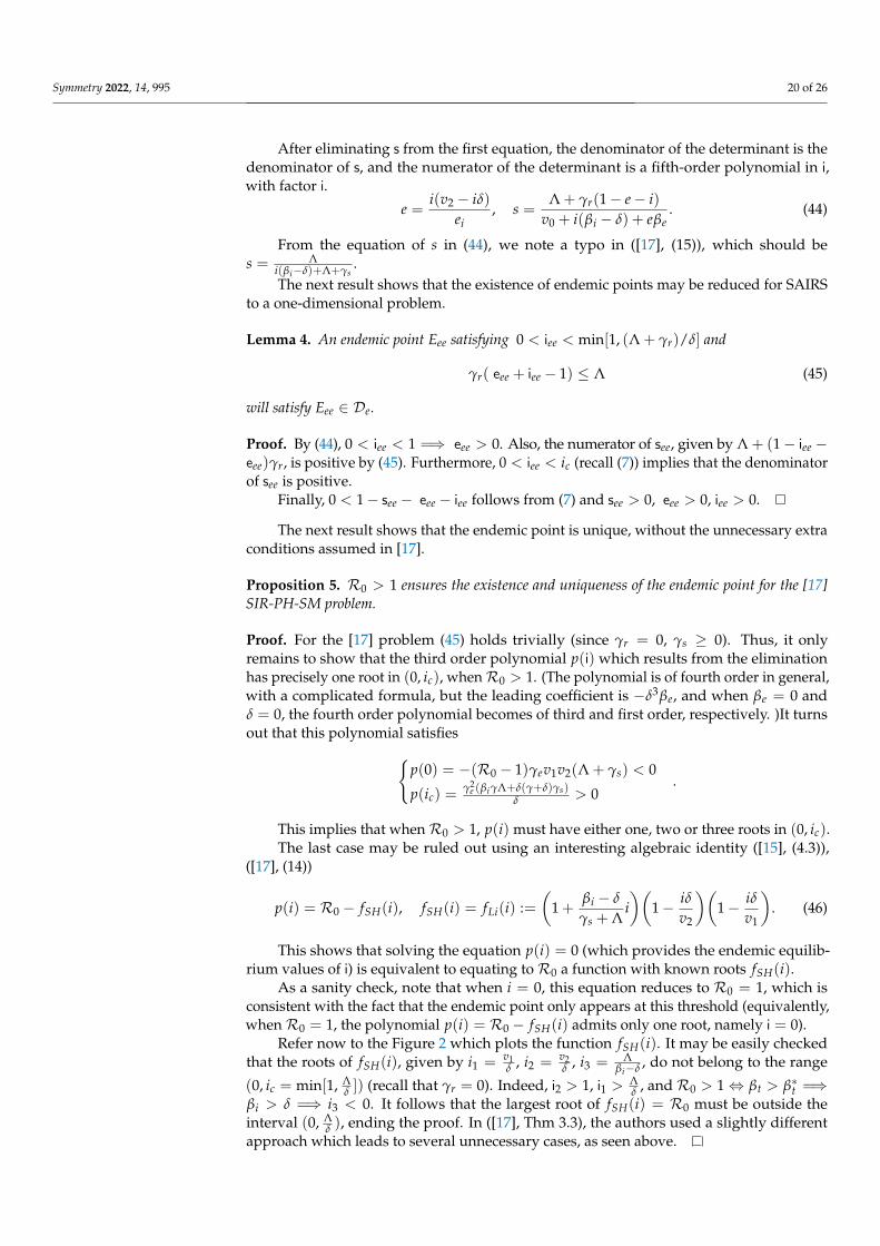
δ ), ending the proof. In ([17], Thm 3.3), the authors used a slightly differentapproach which leads to several unnecessary cases, as seen above.

Symmetry 2022, 14, 995 21 of 26

From the proof above, when R0 > 1, the line f = R0 has exactly one intersection(iee, fSH(iee)) with the graph of fSH(i) that satisfies iee ∈ [0, ic],– see Figure 2.

0.5 1.0 1.5 2.0i

-1

1

2

3

4

f

Λ/ν

{Λ/ν,fSH(Λ/ν)}

fSH(i)

R0

fSH(Λ/ν)

Figure 2. The existence and uniqueness of endemic point iee in the interval [0, ic] for the [17] problem,([15], Figure 1), with fSH(i) as defined in (46), fSH(Λ

δ ) =(γ+δ)γe(βiΛ+δγs)

Λδ(Λ+γ+δ)(v1)(Λ+γs), β = 18, βe = γr = 0,

Λ = 45 and δ = γ = ei = γs = γe = 1.

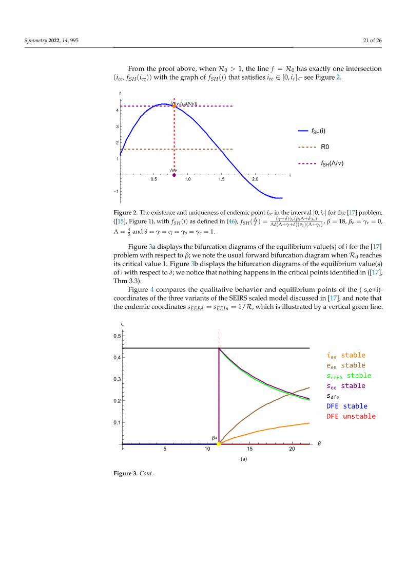
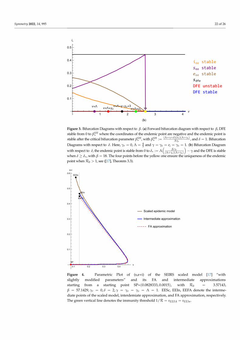
Figure 3a displays the bifurcation diagrams of the equilibrium value(s) of i for the [17]problem with respect to β; we note the usual forward bifurcation diagram whenR0 reachesits critical value 1. Figure 3b displays the bifurcation diagrams of the equilibrium value(s)of i with respect to δ; we notice that nothing happens in the critical points identified in ([17],Thm 3.3).

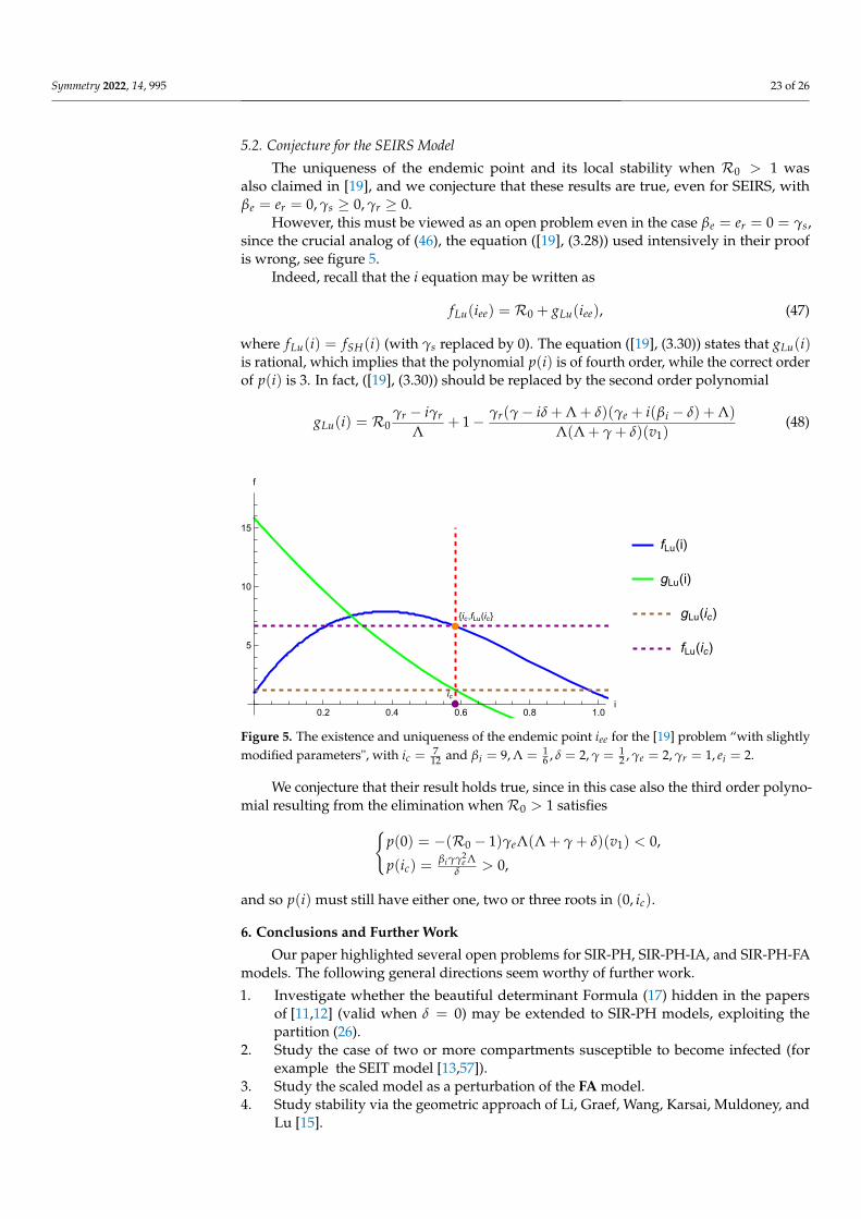
Figure 4 compares the qualitative behavior and equilibrium points of the ( s,e+i)-coordinates of the three variants of the SEIRS scaled model discussed in [17], and note thatthe endemic coordinates sEEFA = sEEIn = 1/R, which is illustrated by a vertical green line.

5 10 15 20β

0.1

0.2

0.3

0.4

0.5

i*

β*

iee stable

eee stable

seeFA stable

see stable

sdfeDFE stable

DFE unstable

(a)

Figure 3. Cont.

Symmetry 2022, 14, 995 22 of 26

1 2 3 4ν

0.1

0.2

0.3

0.4

0.5

i*

ν*ν=Λ

ν>Λ+γsν=Λ-γ-γe+3ν<Λ+γe

iee stable

see stable

eee stable

sdfeDFE unstable

DFE stable

(b)

Figure 3. Bifurcation Diagrams with respect to β. (a) Forward bifurcation diagram with respect to β, DFEstable from 0 to βSH

∗ where the coordinates of the endemic point are negative and the endemic point isstable after the critical bifurcation parameter βSH

∗ , with βSH∗ := (Λ+γ+δ)(v1)(Λ+γs)

Λγe, and δ = 1. Bifurcation

Diagrams with respect to δ. Here, γr = 0, Λ = 45 and γ = γe = ei = γs = 1. (b) Bifurcation Diagram

with respect to δ, the endemic point is stable from 0 to δ∗ := Λ(

βiγe(Λ+γe)(Λ+γs)

)− γ and the DFE is stable

when δ ≥ δ∗, with β = 18. The four points before the yellow one ensure the uniqueness of the endemicpoint whenR0 > 1, see ([17], Theorem 3.3).

0.1 0.2 0.3 0.4s

0.1

0.2

0.3

0.4

0.5

0.6

e+i

SP

EEFA

EESc

EEIn

Scaled epidemic model

Intermediate approximation

FA approximation

Figure 4. Parametric Plot of (s,e+i) of the SEIRS scaled model [17] “withslightly modified parameters” and its FA and intermediate approximationsstarting from a starting point SP=(0.0828333, 0.0015), with R0 = 3.57143,β = 57.1429, γr = 0, δ = 2, γ = γe = γs = Λ = 1. EESc, EEIn, EEFA denote the interme-diate points of the scaled model, interdemiate approximation, and FA approximation, respectively.The green vertical line denotes the immunity threshold 1/R = sEEFA = sEEIn.

Symmetry 2022, 14, 995 23 of 26

5.2. Conjecture for the SEIRS Model

The uniqueness of the endemic point and its local stability when R0 > 1 wasalso claimed in [19], and we conjecture that these results are true, even for SEIRS, withβe = er = 0, γs ≥ 0, γr ≥ 0.

However, this must be viewed as an open problem even in the case βe = er = 0 = γs,since the crucial analog of (46), the equation ([19], (3.28)) used intensively in their proofis wrong, see figure 5.

Indeed, recall that the i equation may be written as

fLu(iee) = R0 + gLu(iee), (47)

where fLu(i) = fSH(i) (with γs replaced by 0). The equation ([19], (3.30)) states that gLu(i)is rational, which implies that the polynomial p(i) is of fourth order, while the correct orderof p(i) is 3. In fact, ([19], (3.30)) should be replaced by the second order polynomial

gLu(i) = R0γr − iγr

Λ+ 1− γr(γ− iδ + Λ + δ)(γe + i(βi − δ) + Λ)

Λ(Λ + γ + δ)(v1)(48)

0.2 0.4 0.6 0.8 1.0i

5

10

15

f

ic

{ic,fLu(ic}

fLu(i)

gLu(i)

gLu(ic)

fLu(ic)

Figure 5. The existence and uniqueness of the endemic point iee for the [19] problem “with slightlymodified parameters", with ic = 7

12 and βi = 9, Λ = 16 , δ = 2, γ = 1

2 , γe = 2, γr = 1, ei = 2.

We conjecture that their result holds true, since in this case also the third order polyno-mial resulting from the elimination whenR0 > 1 satisfies{

p(0) = −(R0 − 1)γeΛ(Λ + γ + δ)(v1) < 0,

p(ic) =βiγγ2

e Λδ > 0,

and so p(i) must still have either one, two or three roots in (0, ic).

6. Conclusions and Further Work

Our paper highlighted several open problems for SIR-PH, SIR-PH-IA, and SIR-PH-FAmodels. The following general directions seem worthy of further work.

1. Investigate whether the beautiful determinant Formula (17) hidden in the papersof [11,12] (valid when δ = 0) may be extended to SIR-PH models, exploiting thepartition (26).

2. Study the case of two or more compartments susceptible to become infected (forexample the SEIT model [13,57]).

3. Study the scaled model as a perturbation of the FA model.4. Study stability via the geometric approach of Li, Graef, Wang, Karsai, Muldoney, and

Lu [15].

Symmetry 2022, 14, 995 24 of 26

5. We hope that the use of more sophisticated and fast software will allow researchers in thefuture to progress with the interesting questions raised by models with higher dimensions.Here, exploiting symmetries may turn out helpful.

Author Contributions: Supervision, Florin Avram; Writing-review and editing, Florin Avram, RimAdenane and Andrei Halanay. All authors have read and agreed to the published version ofthe manuscript.

Funding: This research received no external funding.

Institutional Review Board Statement: Not applicable.

Informed Consent Statement: Not applicable.

Data Availability Statement: Not applicable.

Acknowledgments: We thank Mattia Sensi and Sara Sottile for useful suggestions and referencesand for providing some of the codes used for producing the figures.

Conflicts of Interest: The authors declare no conflict of interest.

References1. Liu, W.m.; Levin, S.A.; Iwasa, Y. Influence of nonlinear incidence rates upon the behavior of SIRS epidemiological models. J.

Math. Biol. 1986, 23, 187–204. [CrossRef] [PubMed]2. Liu, W.m.; Hethcote, H.W.; Levin, S.A. Dynamical behavior of epidemiological models with nonlinear incidence rates. J. Math.

Biol. 1987, 25, 359–380. [CrossRef] [PubMed]3. Vyska, M.; Gilligan, C. Complex dynamical behaviour in an epidemic model with control. Bull. Math. Biol. 2016, 78, 2212–2227.

[CrossRef]4. Roostaei, A.; Barzegar, H.; Ghanbarnejad, F. Emergence of Hopf bifurcation in an extended SIR dynamic. arXiv 2021,

arXiv:2107.10583.5. Gupta, R.; Kumar, A. Endemic bubble and multiple cusps generated by saturated treatment of an SIR model through Hopf and

Bogdanov–Takens bifurcations. Math. Comput. Simul. 2022, 197, 1–21. [CrossRef]6. De la Sen, M.; Nistal, R.; Alonso-Quesada, S.; Ibeas, A. Some formal results on positivity, stability, and endemic steady-state

attainability based on linear algebraic tools for a class of epidemic models with eventual incommensurate delays. Discret. Dyn.Nat. Soc. 2019, 2019, 8959681. [CrossRef]

7. De la Sen, M.; Ibeas, A.; Alonso-Quesada, S.; Nistal, R. On the Carrying and Evolution Matrices in Epidemic Models. J. Phys.Conf. Ser. 2021, 1746, 012015. [CrossRef]

8. Arino, J.; Brauer, F.; van den Driessche, P.; Watmough, J.; Wu, J. A final size relation for epidemic models. Math. Biosci. Eng. 2007,4, 159.

9. Avram, F.; Adenane, R.; Ketcheson, D.I. A review of matrix SIR Arino epidemic models. Mathematics 2021, 9, 1513. [CrossRef]10. Avram, F.; Adenane, R.; Basnarkov, L.; Bianchin, G.; Goreac, D.; Halanay, A. On matrix-SIR Arino models with linear birth rate,

loss of immunity, disease and vaccination fatalities, and their approximations. arXiv 2021, arXiv:2112.03436.11. Robinson, M.; Stilianakis, N.I. A model for the emergence of drug resistance in the presence of asymptomatic infections. Math.

Biosci. 2013, 243, 163–177. [CrossRef] [PubMed]12. Ottaviano, S.; Sensi, M.; Sottile, S. Global stability of SAIRS epidemic models. Nonlinear Anal. Real World Appl. 2022, 65, 103501.

[CrossRef]13. Van den Driessche, P.; Watmough, J. Further notes on the basic reproduction number. In Mathematical Epidemiology; Springer:

Berlin/Heidelberg, Germany, 2008; pp. 159–178.14. Greenhalgh, D. Hopf bifurcation in epidemic models with a latent period and nonpermanent immunity. Math. Comput. Model.

1997, 25, 85–107. [CrossRef]15. Li, M.Y.; Graef, J.R.; Wang, L.; Karsai, J. Global dynamics of a SEIR model with varying total population size. Math. Biosci. 1999,

160, 191–213. [CrossRef]16. Li, M.Y.; Muldowney, J.S. Dynamics of differential equations on invariant manifolds. J. Differ. Equ. 2000, 168, 295–320. [CrossRef]17. Sun, C.; Hsieh, Y.H. Global analysis of an SEIR model with varying population size and vaccination. Appl. Math. Model. 2010,

34, 2685–2697. [CrossRef]18. Britton, T.; Ouédraogo, D. SEIRS epidemics with disease fatalities in growing populations. Math. Biosci. 2018, 296, 45–59.

[CrossRef]19. Lu, G.; Lu, Z. Global asymptotic stability for the SEIRS models with varying total population size. Math. Biosci. 2018, 296, 17–25.

[CrossRef]20. Douris, P.; Markakis, M. Global Connecting Orbits of a SEIRS Epidemic Model with Nonlinear Incidence Rate and Nonpermanent

Immunity. Eng. Lett. 2019, 27, 1–10.

Symmetry 2022, 14, 995 25 of 26

21. Ansumali, S.; Kaushal, S.; Kumar, A.; Prakash, M.K.; Vidyasagar, M. Modelling a pandemic with asymptomatic patients, impact oflockdown and herd immunity, with applications to SARS-CoV-2. Annu. Rev. Control 2020, 50, 432–447. [CrossRef]

22. Graef, J.R.; Li, M.Y.; Wang, L. A Study on the Effects of Disease Caused Death in a Simple Epidemic Model; American Institute ofMathematical Sciences: Springfield, MI, USA, 1998; Volume 1998, p. 288.

23. Ferreira, R.A.; Silva, C.M. A nonautonomous epidemic model on time scales. J. Differ. Equ. Appl. 2018, 24, 1295–1317. [CrossRef]24. Russo, G.; Wirth, F. Matrix measures, stability and contraction theory for dynamical systems on time scales. arXiv 2020,

arXiv:2007.08879.25. Avram, F.; Adenane, R.; Bianchin, G.; Halanay, A. Stability Analysis of an Eight Parameter SIR-Type Model Including Loss of

Immunity, and Disease and Vaccination Fatalities. Mathematics 2022, 10, 402. [CrossRef]26. Goh, B.S. Global stability in many-species systems. Am. Nat. 1977, 111, 135–143. [CrossRef]27. Bacaër, N. Mathématiques et Épidémies. 2021. Available online: https://hal.archives-ouvertes.fr/hal-03331469 (accessed on 20

March 2022).28. Ballyk, M.M.; McCluskey, C.C.; Wolkowicz, G.S. Global analysis of competition for perfectly substitutable resources with linear

response. J. Math. Biol. 2005, 51, 458–490. [CrossRef]29. Fall, A.; Iggidr, A.; Sallet, G.; Tewa, J.J. Epidemiological models and Lyapunov functions. Math. Model. Nat. Phenom. 2007,

2, 62–83. [CrossRef]30. Li, M.Y.; Muldowney, J.S. Global stability for the SEIR model in epidemiology. Math. Biosci. 1995, 125, 155–164. [CrossRef]31. Busenberg, S.; Van den Driessche, P. Analysis of a disease transmission model in a population with varying size. J. Math. Biol.

1990, 28, 257–270. [CrossRef]32. Li, M.Y.; Muldowney, J.S. A geometric approach to global-stability problems. SIAM J. Math. Anal. 1996, 27, 1070–1083. [CrossRef]33. Shuai, Z.; van den Driessche, P. Global stability of infectious disease models using Lyapunov functions. SIAM J. Appl. Math. 2013,

73, 1513–1532. [CrossRef]34. LeVeque, R.J.; Mitchell, I.M.; Stodden, V. Reproducible research for scientific computing: Tools and strategies for changing the

culture. Comput. Sci. Eng. 2012, 14, 13–17. [CrossRef]35. Wang, W. Backward bifurcation of an epidemic model with treatment. Math. Biosci. 2006, 201, 58–71. [CrossRef] [PubMed]36. Tang, Y.; Huang, D.; Ruan, S.; Zhang, W. Coexistence of limit cycles and homoclinic loops in a SIRS model with a nonlinear

incidence rate. SIAM J. Appl. Math. 2008, 69, 621–639. [CrossRef]37. Zhou, L.; Fan, M. Dynamics of an SIR epidemic model with limited medical resources revisited. Nonlinear Anal. Real World Appl.

2012, 13, 312–324. [CrossRef]38. Sun, S. Global dynamics of a SEIR model with a varying total population size and vaccination. Int. J. Math. Anal. 2012,

6, 1985–1995.39. Wiggers, S.L.; Pedersen, P. Routh–hurwitz-liénard–chipart criteria. In Structural Stability and Vibration; Springer:

Berlin/Heidelberg, Germany, 2018; pp. 133–140.40. Anderson, B.; Jury, E. A simplified Schur-Cohn test. IEEE Trans. Autom. Control 1973, 18, 157–163. [CrossRef]41. Daud, A.A.M. A Note on Lienard-Chipart Criteria and its Application to Epidemic Models. Math. Stat. 2021, 9, 41–45. [CrossRef]42. Ma, J.; Earn, D.J. Generality of the final size formula for an epidemic of a newly invading infectious disease. Bull. Math. Biol.

2006, 68, 679–702. [CrossRef]43. Feng, Z. Final and peak epidemic sizes for SEIR models with quarantine and isolation. Math. Biosci. Eng. 2007, 4, 675.44. Andreasen, V. The final size of an epidemic and its relation to the basic reproduction number. Bull. Math. Biol. 2011, 73, 2305–2321.

[CrossRef]45. Georgescu, P.; Hsieh, Y.H. Global stability for a virus dynamics model with nonlinear incidence of infection and removal. SIAM J.

Appl. Math. 2007, 67, 337–353. [CrossRef]46. Hu, Z.; Ma, W.; Ruan, S. Analysis of SIR epidemic models with nonlinear incidence rate and treatment. Math. Biosci. 2012,

238, 12–20. [CrossRef] [PubMed]47. Razvan, M. Multiple equilibria for an SIRS epidemiological system. arXiv 2001, arXiv:math/0101051.48. Yang, W.; Sun, C.; Arino, J. Global analysis for a general epidemiological model with vaccination and varying population. J.

Math. Anal. Appl. 2010, 372, 208–223. [CrossRef]49. Riaño, G. Epidemic Models with Random Infectious Period. medRxiv 2020. [CrossRef]50. Plemmons, R.J. M-matrix characterizations. I—Nonsingular M-matrices. Linear Algebra Its Appl. 1977, 18, 175–188. [CrossRef]51. Hurtado, P.J.; Kirosingh, A.S. Generalizations of the ‘Linear Chain Trick’: Incorporating more flexible dwell time distributions

into mean field ODE models. J. Math. Biol. 2019, 79, 1831–1883. [CrossRef]52. Hyman, J.M.; Li, J.; Stanley, E.A. The differential infectivity and staged progression models for the transmission of HIV. Math.

Biosci. 1999, 155, 77–109. [CrossRef]53. Horn, R.A.; Johnson, C.R. Matrix Analysis; Cambridge University Press: Cambridge, UK, 2012.54. Van den Driessche, P.; Watmough, J. Reproduction numbers and sub-threshold endemic equilibria for compartmental models of

disease transmission. Math. Biosci. 2002, 180, 29–48. [CrossRef]55. Diekmann, O.; Heesterbeek, J.; Roberts, M.G. The construction of next-generation matrices for compartmental epidemic models.

J. R. Soc. Interface 2010, 7, 873–885. [CrossRef]

Symmetry 2022, 14, 995 26 of 26

56. Gasca, M.; Pena, J.M. Total positivity and Neville elimination. Linear Algebra Its Appl. 1992, 165, 25–44. [CrossRef]57. Martcheva, M. An Introduction to Mathematical Epidemiology; Springer: Berlin/Heidelberg, Germany, 2015; Volume 61.