Ph.D Dissertation

UNIVERSITY OF TRENTO

Doctoral School in Mathematics

Human behaviour

in epidemic modelling

Piero Poletti

Advisor:Prof. Andrea Pugliese

Co-Advisor:Dr. Stefano Merler

December 2010

Contents

1 Introduction 5

1.1 Human behavior in response to epidemics . . . . . . . . . . . . . . . . . . . 5

1.2 State of Art . . . . . . . . . . . . . . . . . . . . . . . . . . . . . . . . . . . 7

1.2.1 Spontaneous social distancing during an epidemic outbreak . . . . . 7

1.2.2 Vaccination choices in not compulsory vaccination program . . . . 8

1.3 Innovative aspects . . . . . . . . . . . . . . . . . . . . . . . . . . . . . . . . 10

1.3.1 Spontaneous social distancing . . . . . . . . . . . . . . . . . . . . . 11

1.3.2 Vaccination choices . . . . . . . . . . . . . . . . . . . . . . . . . . . 12

1.4 Structure of the Thesis . . . . . . . . . . . . . . . . . . . . . . . . . . . . . 12

2 Spontaneous behavioral response to an epidemic outbreak 15

2.1 Introduction . . . . . . . . . . . . . . . . . . . . . . . . . . . . . . . . . . 15

2.2 The Model . . . . . . . . . . . . . . . . . . . . . . . . . . . . . . . . . . . 16

2.3 Study of Dynamics . . . . . . . . . . . . . . . . . . . . . . . . . . . . . . . 19

2.4 Discussion . . . . . . . . . . . . . . . . . . . . . . . . . . . . . . . . . . . 28

3 Effectiveness of spontaneous social distancing and risk perception 31

3.1 Introduction . . . . . . . . . . . . . . . . . . . . . . . . . . . . . . . . . . . 31

3.2 The model . . . . . . . . . . . . . . . . . . . . . . . . . . . . . . . . . . . . 32

3.3 Reproductive number and model parametrization . . . . . . . . . . . . . . 34

3.4 Results . . . . . . . . . . . . . . . . . . . . . . . . . . . . . . . . . . . . . . 36

3.5 Discussion . . . . . . . . . . . . . . . . . . . . . . . . . . . . . . . . . . . . 42

4 The effect of risk perception on the 2009 H1N1 pandemic influenzadyanmics 45

4.1 Introduction . . . . . . . . . . . . . . . . . . . . . . . . . . . . . . . . . . . 45

4.2 Materials and Methods . . . . . . . . . . . . . . . . . . . . . . . . . . . . . 46

4.2.1 Data description . . . . . . . . . . . . . . . . . . . . . . . . . . . . 46

4.2.2 The model . . . . . . . . . . . . . . . . . . . . . . . . . . . . . . . . 46

4.3 Results . . . . . . . . . . . . . . . . . . . . . . . . . . . . . . . . . . . . . . 48

4.4 Discussion . . . . . . . . . . . . . . . . . . . . . . . . . . . . . . . . . . . . 53

1

5 Optimal vaccination choice, (static) vaccination games, and rational ex-emption 555.1 Introduction . . . . . . . . . . . . . . . . . . . . . . . . . . . . . . . . . . . 555.2 A simple model of optimal family behavior without strategic interaction . . 57

5.2.1 The case of informed families . . . . . . . . . . . . . . . . . . . . . 585.2.2 Not fully-informed families . . . . . . . . . . . . . . . . . . . . . . 605.2.3 Only a fraction of the population is eligible . . . . . . . . . . . . . 62

5.3 Implications of strategic behavior: the game-theoretic approach . . . . . . 625.3.1 A preliminary: the critical elimination line for multigroup popula-

tions . . . . . . . . . . . . . . . . . . . . . . . . . . . . . . . . . . . 625.3.2 The vaccination game . . . . . . . . . . . . . . . . . . . . . . . . . 635.3.3 The basic strategic competition . . . . . . . . . . . . . . . . . . . . 655.3.4 The Stackelberg case with anti-vaccinators leadership . . . . . . . . 695.3.5 The social planner case . . . . . . . . . . . . . . . . . . . . . . . . 70

5.4 Discussion: can we get off the no-elimination trap? . . . . . . . . . . . . . 73

6 The impact of vaccine side effects on the natural history of immunizationprograms: an imitation-game approach 756.1 Introduction . . . . . . . . . . . . . . . . . . . . . . . . . . . . . . . . . . . 756.2 Materials and Methods . . . . . . . . . . . . . . . . . . . . . . . . . . . . . 76

6.2.1 Dynamic vaccine demand and vaccine side effects . . . . . . . . . . 766.2.2 The importance of time delays . . . . . . . . . . . . . . . . . . . . . 78

6.3 Results . . . . . . . . . . . . . . . . . . . . . . . . . . . . . . . . . . . . . . 796.3.1 Endemic equilibria and their stability . . . . . . . . . . . . . . . . . 796.3.2 Analysis of selected subcases . . . . . . . . . . . . . . . . . . . . . . 81

6.4 Substantive implications of vaccine side effects for vaccination programmes 826.4.1 The epidemiological transition and vaccination payoff . . . . . . . . 826.4.2 Simulations . . . . . . . . . . . . . . . . . . . . . . . . . . . . . . . 83

6.5 Concluding remarks . . . . . . . . . . . . . . . . . . . . . . . . . . . . . . . 88

7 Conclusion 91

8 Appendix 978.1 Appendix A . . . . . . . . . . . . . . . . . . . . . . . . . . . . . . . . . . . 97

8.1.1 Proofs . . . . . . . . . . . . . . . . . . . . . . . . . . . . . . . . . . 978.2 Appendix B . . . . . . . . . . . . . . . . . . . . . . . . . . . . . . . . . . . 101

8.2.1 The model . . . . . . . . . . . . . . . . . . . . . . . . . . . . . . . . 1018.2.2 Sensitivity analysis . . . . . . . . . . . . . . . . . . . . . . . . . . . 1048.2.3 Alert time . . . . . . . . . . . . . . . . . . . . . . . . . . . . . . . . 1098.2.4 Analysis of past influenza seasons . . . . . . . . . . . . . . . . . . . 1098.2.5 Analysis of epidemiological and virological surveillance data . . . . 112

8.3 Appendix C . . . . . . . . . . . . . . . . . . . . . . . . . . . . . . . . . . . 1148.3.1 Properties and more details . . . . . . . . . . . . . . . . . . . . . . 114

2

Bibliography 115

3

4

Chapter 1

Introduction

1.1 Human behavior in response to epidemics

Mathematical models represent a powerful tool for investigating human infection dis-eases, providing useful predictions about the potential transmissibility of a disease andthe effectiveness of possible control measures.

As well known, the characteristics of the pathogen responsible for the infections [6, 19]play a central role in the spread of an infectious disease. Nonetheless, one of the mostcentral aspects of the human infection dynamics is the heterogeneity in behavioral pattersadopted by the host population. Actually, the role played by human mobility patterns [84,38, 151, 11, 112], the sociodemographic structure of the population [112] and interventionmeasures [6, 92] has been deeply investigated.

However, changes in human behaviors caused by the reaction to the disease can playa crucial role as well [56, 52]. Beyond behavioral changes imposed by public authorities,human behavioral changes can be triggered by uncoordinated responses driven by riskperception and fear of diseases (eventually of unknown fatality). Indeed, some studies onrecent outbreaks of infectious disease have shown that people are prone to reduce riskybehaviors [144, 98, 90, 125].

While behavioral responses to the spread of a diseases have been frequently reportedanecdotally, there has been relatively little systematic investigation into their nature andon how they can affect the spread of infectious diseases. Behavioral changes are sometimescited in the interpretation of outbreak data to explain drops in the transmission rate [132,121], yet rarely spontaneous behavioral changes are explicitly modeled and investigated.

Efforts to study human behavior in the context of epidemics usually concentrated onevaluating the effectiveness of various institutionally enforced measures such as schoolclosures [21, 80, 28, 27]. Recently, however, the impact of self-protective actions on thedynamics of an infectious disease has received increased attention [147, 42, 53, 93, 67,66, 17, 15, 16, 29, 48, 47, 49, 45, 108, 61, 131, 69, 129, 72, 127, 130]. In fact, humanspontaneous responses to an epidemic can affect remarkably the infection spread, andtheir interactions with disease dynamics require a proper investigation in order to bet-ter understand what happens when a disease spreads through human populations [56, 52].

5

With spontaneous behavioral responses here we define the changes in human behavioralpatterns that involve personal decisions based on the available information about thedisease or on individuals’ beliefs and attitudes. This phenomenon is completely differentfrom scenarios where the public is expected to comply with recommendations or controlmeasures imposed by institutions.

Common childhood diseases, such as chickenpox and measles, provide a suitable ex-ample of when personal decisions are relevant. In fact, the decision whether or not tovaccinate a child is ultimately a personal decision and thus it has a strong behavioralcomponent. Similarly, it is reasonable that during a severe epidemic outbreak individualstry to reduce the number of potentially infectious contacts. The avoidance of crowdedenvironments, usage of face masks, practice of better hygiene protocols and self-restrictionin traveling represent examples of self-imposed measures that can remarkably affect thedisease spread.

During the 1918 influenza pandemic people eventually stayed away from congregatedplaces [40]. In 1995, a supposed outbreak of bubonic plague in Sura, India, causedwidespread panic on hundreds of thousands of people remarkably changing their trav-eling patterns [24]. When the Severe Acute Respiratory Syndrome (SARS) emerged in2003, the usage of face masks became widespread in affected areas [98], and many indi-viduals changed their traveling behavior [98, 58]. More recently, a high risk perception,possibly as a consequence of the exposure to a massive information campaign (media) onthe risks of an emerging influenza pandemic, was detected during the 2009 H1N1 pan-demic influenza [90] and, despite the low fatality associated to the event [128], behavioralresponse apparently played a relevant role during the early stages of the pandemic aswell [144]. On the other hand, it was observed an increase in protective behavior as theprevalence of the disease was increasing, for both measles [125] and HIV [2]. Finally,concerns about proclaimed risks of vaccines have probably driven a widespread refusalof vaccination, leading to drops in vaccine uptake. This was the case of pertussis in the1970s [70] and more recently of measles-mumps-rubella (MMR) vaccine [89].

As a matter of fact, attitudes, belief systems, available information about the riskassociated to a disease can change over time. The dynamics of these attributes is a rel-evant element to understand the impact of behavioral responses to a disease [68]. Thus,infection dynamics should be considered as a coupled dynamics where the transmission ofthe pathogen is driven by human behavior dynamics, and vice versa. The investigation ofthis complex interplay would be helpful for giving insight to public health policy makers,for planning public health control strategies (e.g., vaccination) and better estimating theburden for health care centers over time.

Two specific phenomena are discussed in this thesis. The first one is represented byvaccination choices during a not compulsory vaccination program for childhood diseases.The second one is represented by spontaneous social distancing during an emerging epi-demic outbreak.

By a modeling point of view, effects of spontaneous behavioral responses on the infec-

6

tion dynamics are very different in these two specific situations. Vaccination may resultin moving individuals directly from the susceptible compartment to the removed com-partment, i.e. those individuals that have developed immunity for the disease. On theother hand a reduced exposure to diseases, as a reaction to the presence of either thedisease or certain beliefs about the disease, could be modeled either as a reduction inthe number of contacts (e.g., reduced travel behavior), or as a reduction of intensity ofcontacts (e.g., usage of face mask). Thus models dealing with spontaneous social distanc-ing, usually, assume a change in parameters (mainly the transmission rate or the recoveryrate) or changes in population structure. Moreover, unless one considers vaccines thatrequire boosting at regular intervals because of waning immunity or because of pathogenevolution ( e.g. seasonal influenza), the decision to vaccinate is usually not reversible. Onthe opposite, social distancing triggered by risk perception, may depend on the dynamicsof the risk of infection.

1.2 State of Art

There are various ways to model behavioral changes over time. Different assumption canbe made not only on the effect of behavioral changes on the epidemic dynamics, butalso on source and type of available information and the way the information spreads inthe population. In addition, more sophisticated models can explicitly include spatial orcontact network structure. In this case behavioral response to epidemics can change inthe network structure as well.

1.2.1 Spontaneous social distancing during an epidemic out-break

A number of studies have considered extensions of the simple SIR model in which theincidence rate is not bilinear in susceptible and infective individuals, but is modeledthrough a more general function, to include effects of saturation. Basically, the assumptionis that, in the presence of a very large number of infective individuals, the population maytend to reduce the number of contacts per time [25]. These models have been shown toyield rich complex dynamics [101, 100], but human behavior and its dynamics are notexplicitly modeled in order to account for a specific reaction to the disease [68].

Arguably, also behavioral response which affects the disease transmission can spreadamong individuals. Recently a class of models accounting for such phenomenon has beenproposed. Such models share the idea that the spread of responsiveness is driven by thediffusion of fear, which can be modeled as a parallel infection [147, 42, 53, 93, 67, 66].

In [147], two different types of behaviors, labeled as “careful” and “risky”, are con-sidered and their frequencies in the population change over time according to social in-teractions. Interestingly, this work shows that responsive behavior (i.e. behavior whichwould guarantee a better protection from the disease and labeled as “careful”) has aninherent evolutionary advantage if riskier behavior leads to faster progression to infection

7

and death. In general, the impact on disease dynamics can be quite remarkable if protec-tive behavior is triggered by fear or awareness of a disease spread. In [53] it is assumedthat people remove themselves from the circulation of a disease completely when they areaffected by fear from the epidemic; in this case the modeled infection dynamics can lead tomultiple epidemic waves as a consequence of the subsequent return into circulation of theindividuals, as fear decreases [53]. In [93], it is assumed that individuals avoid infection orseek treatment earlier as they become aware of a disease; as a consequence, the diffusionof health information can reduce the prevalence of infection. In [42], behavioral responsescan produce a reduction in both the basic reproductive number of the disease and thefinal epidemic size as a consequence of people entering a class of low activity at a givenrate depending on the prevalence of a disease.

As for models involving more complex structures, if susceptibility of individuals isreduced as a direct consequence of having infectious contacts in a social network, it hasbeen shown that a disease can be brought to extinction when self-protection is strongenough [9]. Moreover, it was shown that behavioral response results particularly effectivewhen the network of information spread overlaps with the contact network of diseasetransmission [67, 66].

The behavior of infected individuals has also been considered in several works [77, 141,167]. The underlying idea is that individuals that develop symptoms alter their contactpatters as a consequence of their sickness. More specifically, models based on contactnetwork assume that individuals who stay at home or avoid infected peers can be seenas cutting links of possible contagion. For instance, in [77, 141, 167], it was assumedthat healthy individuals completely remove contacts with infected peers (eventually re-connecting them with the rest of the population). However, changing network structureremoving only existing link is often unrealistic (e.g., it could be “realistic” only in thespecific context of sexually transmitted diseases). The effect of cutting links of possiblecontagion is very similar to a reduction in the transmission rate [68].

1.2.2 Vaccination choices in not compulsory vaccination pro-gram

Vaccination policies of a large number of countries are based on voluntary compliance[68]. Some recent outbreaks of vaccine preventable diseases occurred in groups opposingvaccination on ideological grounds [79] or in communities beyond the reach of health careauthorities [35]. Although forms of exemption to vaccination have always existed [139],the natural history of vaccination programs has always been pervaded by a high degree ofoptimism [29]. However, this optimistic view has increasingly been challenged in recentyears. Indeed, concerns about proclaimed risks of vaccines can produce widespread refusalof vaccination and consequent drops in vaccine uptake.

For example, opposition to the whole-cell pertussis vaccine in the 1970s [70], thethimerosal case [106], and more recently the MMR scare [89, 135, 64, 142, 163] can beconsidered evidence that, in industrialized countries, the success story of vaccination isfeeding back on itself. This is the consequence of two different processes. On the one

8

hand, the high degree of herd immunity achieved by decades of successful immunizationprograms has reduced the incidence of many infections to negligible levels. On the otherhand, the large, and increasing, number of vaccines routinely administered every yearyields steady flows of vaccine-associated side effects [160, 159]. In the US approximately30,000 reports of Vaccine Adverse Events are notified annually, with 10–15% classified asserious [62]. In such circumstances the perception of the public will likely rank the per-ceived risk of suffering a vaccine side effect (VSE) as much higher than the correspondingrisk of infection.

A common example is poliomyelitis in industrialized countries. In Italy during 1980-2000 the number of vaccine-induced polio cases was three times higher than wild poliocases [43]. In addition, it is well known that there can be a significant imbalance betweenperceived and real risk. An example of misperception of risk is the belief that the MMRvaccine can cause autism [120, 146]. In fact, such belief has spread widely despite theoverwhelming evidences that reject such a causality [146].

Drops in vaccination coverage have led to increased interest in so-called rational vac-cination decisions and their effects on the epidemiology of vaccine preventable infectiousdiseases. Many epidemiological modelers have turned to game theory and focused on thedilemma introduced by voluntary vaccination.

The “free riding” problem and the rational exemption in vaccination

Under voluntary vaccination high degrees of herd immunity might incentives vaccinationfree riding [145, 23, 131].

The name “free rider” comes from a historical example for public transportation:people using a bus without paying the fare are free riders. The free rider problem raiseswhen too many individuals becomes free riders and thereby the system has not enoughmoney to operate. Herd immunity consists in the indirect protection for unvaccinatedindividuals provided by vaccinated individuals, as the latter will not contract and transmitthe disease. The notion of free riding in vaccination means that, if vaccination is perceivedto come with risk or side-effects, the better strategy can appear not vaccinating, thusavoiding any risk of vaccine side effects, while relying on the rest of the population tokeep the coverage high enough to provide herd immunity.

The rational exemption, as defined in [48, 108], represents the parents’ decision not toimmunize children after a seemingly “rational” comparison between the perceived utilityof vaccination, i.e. protection from the risk of infection – perceived as very low as aconsequence of the high herd immunity due to decades of successful vaccination policies– with its disutility, i.e. the risk of vaccine associated side effects. Actually, a behavior,resulting from the optimization performed by rational agents, might well turn out to bemyopically rational, since it considers only the current perceived risk of disease, and notthe risk of its future resurgence due to declining coverage. Several evidence of rationalexemption behavior are documented by surveys of vaccination lifestyles [8, 107, 163, 64].

A series of recent intriguing works have attempted to explain rational exemption inits most appropriate framework, i.e. game theory [16, 15, 36, 131]. These papers have

9

provided the first game-theoretic proof of the elimination impossible result, and variousimplications of rational exemption. These implications suggest potential difficulties forglobal eradication plans, both at the national and international level [13, 55].

The game theoretical approach

When vaccination decisions are investigated using the game theory framework, it canbe shown that the vaccination level attained from individuals acting only in their bestself-interest is always below the optimal for the community. This result implies that it isimpossible to eradicate a disease under voluntary vaccination [17, 15, 16, 29, 48, 23, 61,48, 47, 49, 45, 131, 69, 129, 69, 72].

Moreover, models based on game theory have shown that the coupled dynamics of vac-cination coverage and disease prevalence can lead to oscillations with outbreaks followingupsurges in vaccination coverage and subsequent epidemic troughs. Such results comesfrom the assumption that vaccination decisions are made by imitating other individualsat a rate depending on the individual benefit [15, 131]. Actually, similar results have alsobeen found by assuming that decisions are based on past prevalence of a disease (e.g. byconsidering time delays and memory mechanisms [131, 150, 48, 49, 22, 45]).

Works focusing on influenza [69] and on human papillomavirus (HPV) [14], in whichthe model is parametrized using the results of population surveys, confirmed the problemthat, with individuals acting rationally according to their perceived risk, the populationdoes not achieve vaccination levels that minimize disease prevalence in the population.Moreover, a similar approach (leading to similar results) has been applied to the studyof vaccination against smallpox to prepare for bioterrorism [17], to childhood diseases[16, 48, 49], to seasonal influenza [150] and to yellow fever [34].

However, it was recently suggested that elimination might become possible when morerealistic contact network structures are considered [124]. Specifically, in [124] it has beenshown that voluntary ring-vaccination of individuals can reduce local outbreaks if contactsare sufficiently local and the response is fast enough.

Beyond investigations based on game theory framework, models have recently beenproposed to base vaccination behavior on the spread of opinions in a social neighborhoodrather than assuming individual rational behavior. In that case, it was shown that clustersof unvaccinated individuals can make outbreaks more likely to occur [138, 50].

1.3 Innovative aspects

Spontaneous human behavioral response is rarely considered explicitly in epidemic mod-eling. This Ph.D. thesis attempts to shed some light on the potential impact of behavioralchanges on infection dynamics. Spontaneous social distancing is investigated in order toassess how and when behavioral changes can affect the spread of an epidemic. As a secondtopic, the problem of rational exemption is faced in order to investigate whether vaccinepreventable diseases can be eliminated through not compulsory vaccination programs.

10

1.3.1 Spontaneous social distancing

While the game theoretical approach has been shared by many modelers for investigatingthe problem of vaccination choices, to the best of my knowledge, no efforts, but for a veryrecent ones [130], were developed for investigating spontaneous social distancing duringan outbreak by using this framework. Moreover, still few works, e.g. [15], deal with theevolutionary game theory framework, instead of considering classic and static games. Theapproach of considering dynamical games allows to explicitly model the coupled dynamicsof disease transmission and behavioral changes based on the risk perception.

Actually, most models accounting for spontaneous social distancing, assume a priorihuman response to the infection or consider only the behavioral response induced bythe diffusion of fear, which is modeled as a parallel infection [42, 147, 53, 93, 67, 66].However, an alternative mechanisms can contribute to the diffusion of responsiveness ina population. In fact, information diffusion may also spread through person to personcontacts and can be modeled as an imitation process in which the convenience of differentbehaviors depends on the perceived risk of infection [9, 52].

Other novelties introduced in this thesis consist in considering: (i) asymptomatic in-fective individuals’ behavior in response to the risk of infection; (ii) the effect of riskmisperception; (iii) time delays and memory mechanisms in the risk perception of infec-tion;

An innovative, in my opinion, aspect of this thesis is the investigation of an actualepidemic through a theoretical model explicitly considering human behavior. Indeed,the application to the 2009 H1N1 pandemic influenza may represent a further step toempirically assess quantitative and qualitative effects of spontaneous human response toperceived risk of infection.

Actually, most modeling efforts undertaken so far to study the impact of human be-havior on the spread of infectious diseases are based on anecdotal evidence and commonsense. Such models are almost never validated against quantifiable observations. Undeni-ably, a lot of data would be needed for model validation and parametrization. Recently,in order to answer questions like “where people obtain their information from”, “whichof information available to them they trust”, “if and how they act upon the information”and “how-effective this reaction is”, several surveys have been performed [98, 90, 82, 39].However, even if many works share the insight on the effect of behavioral response on theepidemic spread, it is still difficult quantify human behavior with robust estimates [68].Nonetheless, coupling the analysis of epidemiological data with drug purchase data, asdiscussed in chapter 4, could represent a promising solution.

At the current stage, proposed models could hardly be used for real time predictionssince our knowledge on model parameters related to human behavior is only preliminary.However, further investigations, perhaps including results coming from surveys, can leadto gain a major consciousness on how spontaneous human behavior could affect epidemicdynamics.

11

1.3.2 Vaccination choices

Vaccination choices are investigated in chapters 5, 6 through different frameworks and as-sumptions, e.g. by considering families as representative agents and investigating differentstatic and dynamic games.

Recent literature has highlighted that human perception of risk plays a central rolein the dynamics of vaccination choices [17, 15, 16, 29, 48, 23, 61, 48, 47, 49, 45, 131, 69,129, 69, 72], and thus strongly affects the chance of diseases’ elimination. As discussed insec. 1.2, elimination of vaccine preventable diseases becomes a challenge when vaccine areperceived as risky. Actually, the mismatch between subjective and objective assessment ofrisk has been demonstrated experimentally [166] and some of the key factors contributingto this mismatch have been deeply investigated [65, 91].

One innovative aspect of proposed models is represented by considering misperceptionof risks induced by partial or incorrect information, both concerning the infection andvaccine side effects. Actually, the imbalance between perceived and real risk play a cen-tral role in determining the possibility of eliminating a vaccine preventable disease. Forexample, the investigation carried out in chapter 5 highlight that elimination turns outto be possible when individuals are not fully informed about herd immunity or about theexistence of a critical vaccination coverage.

Other novelties introduced in this thesis consist in considering: (i) the case of hetero-geneous predisposition to vaccinate, assuming the population divided in groups that havedifferent perceptions about risk of VSEs; (ii) nonlinear perceived costs of infection; (iii)the possibility that the perceived costs of infection and vaccination are evaluated by thepublic using past values of state variables, for example due to information delay or of theperception of long-term vaccine side effects.

The model introduced in chapter 6 makes, in my opinion, useful contributions to theinvestigation of the problem of rational exemption. The main innovation is to modelthe perceived risk of vaccination as a function of the incidence of vaccine side effects. Ifavailable information on vaccine side effects is becoming the main driving force of vaccinedemand, as strongly supported by empirical evidence [135], this work may represent anappropriate description of the future evolution of immunization programs in voluntaryvaccination regimes.

1.4 Structure of the Thesis

This thesis is structured as follows. In the next chapter, a simple model coupling anSIR transmission process with an imitation process is introduced in order to investigateeffects of spontaneous social distancing during an epidemic outbreak. Specifically, themodel assume that individuals are able to reduce their susceptibility. The potential im-pact of behavioral response on the final epidemic size and the temporal dynamics of theepidemic is assessed, and the chance of multiple epidemic waves is discussed. An accuratetheoretical investigation is also carried out, capturing essential patterns of the infectiondynamics when behavioral changes are much faster than the epidemic transmission.

12

In chapter 3, an extension of the model presented in chapter 2 is described. Bothbehavioral response performed by infected individuals and the effect of a memory mecha-nism in perception of risk are considered. The aim of this chapter is to investigate whenand how the behavioral response affects the epidemic spread, clarifying the role of thekey features describing human response. Moreover, scenarios accounting for the chanceof delayed warning and behavioral responses triggered by the misperception of risk areanalyzed.

In chapter 4, this approach is applied for investigating the specific case of the 2009H1N1 pandemic influenza in Italy. The chapter is mainly focused on the analysis ofreal datasets. The hypothesis of an initial overestimation of risk by the host populationis advanced, as a plausible explanation for the unusual and notable pattern observablein the ILI incidence reported to the national surveillance system. Such hypothesis issupported by empirical evidences, such as the temporal pattern of drug purchase and some(sporadic) reactive school closure (“self-imposed” by the scholastic board or suggested bylocal authorities).

Chapter 5, is devoted to the discussion of the problem of rational exemption in de-veloped countries, through a set of simple static models for vaccination behavior. Firstlythe problem is investigated trough the hypothesis of representative agent and, secondly,considering game strategic interactions, including the Stackelberg competition and theanalysis of Nash Equilibria. The case of partial information about the risk of an epi-demic is considered and the effect of heterogeneity in the perception of risks associatedto vaccination is investigated as well.

In chapter 6, a transmission model with dynamic vaccine demand based on an imita-tion mechanism and with the perceived risk of vaccination modeled as a function of theincidence of VSEs is introduced. The analysis of the equilibria is performed and notewor-thy inferences as regards both the past and future lifetime of vaccination programs aredrown.

Finally, in chapter 7 includes a summary of work made during the thesis projectand a discussion on several open issues about human spontaneous behavior in epidemicmodeling.

13

14

Chapter 2

Spontaneous behavioral response toan epidemic outbreak

2.1 Introduction

The epidemic dynamics depends on the complex interplay between the characteristics ofthe pathogens’ transmissibility and the structure and behaviour of the host population.Spontaneous change of behaviour in response to epidemics [56], possibly related to riskperception [9, 133, 141], has been recently proposed as a relevant factor in the compre-hension of infection dynamics. While the merits and influence of such phenomena arestill debated [48, 117], experience from the 1918-19 pandemic indicates that a better un-derstanding of behavioural patterns is crucial to improve model realism and enhance theeffectiveness of containment/mitigation policies [21].

Human behaviour is driven by evaluation of prospective outcomes deriving from alter-native decisions and cost-benefit considerations. Past experience, response to the actionof others and changes in exogenous conditions all contribute to the balance, to whichgame theory provides a rich and natural modelling framework [154, 81]. It is not surpris-ing, therefore, that looking at behaviours through the lens of game theory has recentlyattracted the attention of the epidemiology community, for example when modelling theevolution over time of voluntary vaccination uptakes [16, 15].

In this paper we model a fairly general situation in which a population of individualsis subject to an epidemic outbreak developing according to an SIR model, but in whichcontact rates depend on the behavioural patterns adopted across the population. Morespecifically, all susceptible individuals can conform to either one or the other of twodifferent behaviours, ba and bn, respectively corresponding to an “altered” and a “normal”behavioural pattern. The first gives the individuals an advantage in terms of reduced riskof infection, yet at some extra cost. For example, avoidance of crowded environmentsreduces the risk of infection, but also entails disadvantages deriving from greater isolation.Individuals adopting the second (bn) are exposed to a normal risk of infection, but arespared the extra cost associated with ba. Individuals may choose to switch between ba andbn at any time, depending on cost-benefit assessments based on the perception of risk.

15

The resulting model consists in the coupling of two dynamical systems, one describingthe epidemic transmission and the other describing the behavioural changes. In principle,there is no reason for the two phenomena to evolve at the same speed. It is thereforecrucial to study the model allowing for different time–scales, embodied in different time-units.

We give a full description of the model when the dynamics of the behavioural changesare “fast” with respect to the epidemic transmission. In particular, we provide sufficientconditions on the parameters for generating sequences of epidemic waves. Moreover, weshow that the model is able to account for “asymmetric waves”, i.e., infection waveswhose rising and decaying phases differ in slope. However, similar patterns can also beobserved when the time–scales of the two dynamics are comparable. When the dynamicof behavioural changes is “slow”, the model basically reduces to a classical SIR.

The model’s dynamics gives rise to patterns that are morphologically compatible withmultiple outbreaks and the same-wave asymmetric slopes recently reported for the Spanishinfluenza of the 1918–19 [32, 31, 58, 115]. For these phenomena (trivially incompatiblewith the classical SIR model) a variety of alternative explanations have in fact beenadvanced: military demobilization at the end of the First World War [58], genetic variationof the influenza virus [26, 7, 20], exogenous time changes in transmission rates, such asseasonal forcing [38, 37]. Other explanations have been proposed invoking coinfectionscenarios [111, 1, 51, 114]

Finally, and regardless of the relative speeds of dynamics, we show that the fractionof susceptible individuals at the end of the epidemic is always larger than that of aclassical SIR model in which all individuals adopt the normal behaviour (bn) with thesame parameters.

2.2 The Model

Our model consists of the coupling of two mutually influencing phenomena: a) the epi-demic transitions; b) the behavioural changes in the population of susceptible individuals.

As for the epidemic transitions, whose time unit is t, our model is based on an S → I →R scheme1. We consider that susceptible individuals may adopt two mutually exclusivebehaviours, bn (“normal”) and ba (“altered”). Specifically, we assume that individualsadopting behaviour ba are able to reduce the number of contacts in the time unit withrespect to individuals adopting behaviour bn. Thus, two transmission rates are consideredfor the two groups, accounting for the different contact rates associated with behavioursba and bn. In particular, susceptible individuals adopting behaviour bn, Sn(t), becomeinfected at a rate βnI(t) (and thus Sn(t) = −βnSn(t)I(t)), where I(t) represents the pool ofinfectious individuals, while susceptible individuals adopting behaviour ba, Sa(t), becomeinfected at a rate βaI(t) (and thus Sa(t) = −βaSa(t)I(t)), with βa < βn. Introducingthe variables S(t) = Sa(t) + Sn(t) and x(t) = Sn(t)/(Sn(t) + Sa(t)), corresponding to the

1Since we model single epidemic outbreaks, the vital dynamics of the population is not taken intoaccount.

16

whole susceptible population and to the fraction of susceptibles adopting behaviour bnrespectively, the epidemic model can be written as:

dS

dt(t) = − [βnS(t)x(t) + βaS(t)(1− x(t))] I(t)

dI

dt(t) = [βnS(t)x(t) + βaS(t)(1− x(t))] I(t)− γI(t)

dR

dt(t) = γI(t)

dx

dt(t) = x(t)(1− x(t))(βa − βn)I(t) .

(2.1)

Notice that the last equation describes the change of behaviours distribution in sus-ceptible individuals deriving from the different rates of infection, βn and βa.

We now allow susceptible individuals to change their behaviour spontaneously, follow-ing cost/benefit considerations. This phenomenon can be cast in the language of evo-lutionary game theory, in which behaviours correspond to strategies in a suitable game,with certain expected payoffs. Adopting ba reduces the risk of infection, but it is morecostly. On the other hand, individuals adopting bn are exposed to a higher risk of infec-tion. It is clear that whether it is more convenient to adopt the first behaviour or thesecond depends on the state of the epidemic.

Of course, the two phenomena may not have the same time scales. In fact, whileepidemic transmission can occur only through person-to-person contacts, it is fairly rea-sonable to consider that individuals can access the information required to decide whetherto adopt either bn or ba, much more frequently by telephone, email, the Internet and, ingeneral, the media.

Let us therefore introduce τ as the time unit of behavioural changes, and let us assumethat t = ατ with α > 0.

Payoffs can now be modelled as it follows. All individuals pay a cost for the riskof infection, which we assume depends linearly on the fraction of infected individuals,I(τ), and it is higher for bn than for ba. Moreover, individuals playing ba pay an extra,fixed cost k. It may be convenient to think of k as deriving from reducing the contactswith people, and therefore less traveling, working, attending school, visiting friends andrelatives, etc.. Yet, it is more general than that, as it can account, in fact, for the cost ofany self-imposable prophylactic measure. The payoffs associated with bn and ba are:

pn(τ) = −mnI(τ)pa(τ) = −k −maI(τ) ,

(2.2)

withmn > ma. We may think ofmn andma as parameters related to the risk of developingsymptoms (especially for the lethal infections) induced by the two different behaviours bnand ba.

17

The dynamics of behaviours is modelled as a selection dynamics based on imitation(Imitation Dynamics [81, 122]). A fraction of the individuals playing strategy bn canswitch to strategy ba after having compared the payoffs of the two strategies, at a rateproportional to the difference between payoffs, ∆P (τ) = pn(τ)− pa(τ), with proportion-ality constant ρ. Conversely for the fraction of the individuals playing ba.

The last equation of system (2.1), in the time scale of infection transmission, thusbecomes:

(2.3)

dx

dt(t) = x(t)(1− x(t))(βa − βn)I(t)+

+ρ

αx(t)(1− x(t))(k − (mn −ma)I(t)) .

Notice that the first component of the time derivative of x(t) is negative, meaningthat the fraction of susceptible individuals adopting the normal beahviour bn can onlydecrease over time as an effect of the selection of behaviours induced by the epidemic. Onthe other hand, whenever bn is more convenient than ba (pn(t) > pa(t)), the fraction inthe population of susceptibles playing bn can grow.

Let us briefly comment on the second component of the time derivative of x(t). Inprinciple, since the number of susceptible individuals decreases over time, one can arguethat spontaneous changes of behaviour must depend explicitly on S(t), because of thediminished number of contacts among susceptible individuals. However, here we assumethat susceptible individuals take their decision on the basis of the composition of thepool of susceptible individuals that they are able to meet somehow (by looking only atthe fractions of susceptible individuals adopting the two behaviours bn and ba, withoutconsidering the size of the sample).

It is worth noticing that x = 0 and x = 1 are equilibria for Eq. (8.7). This in particularimplies that there is no way to switch to a different strategy (independently of whetherit would be convenient) unless there is a non zero fraction of individuals already playingit. To circumvent this (which one may regard as an undesirable effect of strict imitation),irrational behaviour can be introduced which allows for rare (in τ time units) randomswitches of behaviour independent of encounters. Assuming a constant rate, χ > 0, equalfor both behaviours, the resulting equation for x is:

(2.4)

dx

dt(t) = x(t)(1− x(t))(βa − βn)I(t)+

+ρ

αx(t)(1− x(t))(k − (mn −ma)I(t))+

+χ

α(1− x(t))− χ

αx(t) .

Therefore, the complete dynamics of infection (coupling behaviour with epidemic tran-

18

Table 2.1: Model variables and parametersNotation Description

S Fraction of susceptible individualsI Fraction of infectious individualsR Fraction of recovered individualsx Fraction of susceptibles individuals adopting the “normal”

behaviourβn Transmission rate of individuals adopting the “normal”

behaviourβa Transmission rate of individuals adopting the “altered”

behaviourγ Recovery rate

1/m Threshold value determining the switch between “normal”and “altered” behaviour

µ Irrational behaviour rateε Relative speed of SIR dynamics and behavioural response

sitions) is given by:

dS

dt(t) = − [βnS(t)x(t) + βaS(t)(1− x(t))] I(t)

dI

dt(t) = [βnS(t)x(t) + βaS(t)(1− x(t))] I(t)− γI(t)

dR

dt(t) = γI(t)

εdx

dt(t) = x(t)(1− x(t))(1−mI(t)) + µ(1− 2x(t)) .

(2.5)

where ε =α

kρ, m = (mn − ma)/k + ε(βn − βa) and µ =

χ

kρ. As for the constraints

on the models parameters, we have: 0 < βa < βn, 0 < γ < βn2, ε > 0, m > ε(βn − βa)

and µ > 0. For facilitating the reader’s understanding, the definitions of the variablesrecurring throughout the paper are reported in Tab. 2.1.

2.3 Study of Dynamics

System (2.5) admits the disease free equilibrium (S, I, R, x) = (1, 0, 0, x?)3, with

(2.6) x? =1− 2µ+

√1 + 4µ2

2,

2This constraint is required only to ensure that the epidemic occurs (see Eq. 3.3).3System (2.5) admits a continuum of equilibria, namely (S?, 0, 1− S?, x?) with S? ∈ [0, 1]. However,

here we consider in detail only the “pandemic” case S? = 1.

19

which is unstable when βnx?+βa(1−x?) > γ. Thus, we assume that the initial values for

system (2.5) are the following: (S(0), I(0), R(0), x(0)) = (1− I0, I0, 0, x?) with I0 close to

0. Note that 1/2 < x? < 1 and x? → 1 when µ → 0. Moreover, this equilibrium is stableas long as R0 < 1 where the basic reproductive number of system (2.5) is:

(2.7) R0 =βnx

? + βa(1− x?)

γ.

Let us introduce the basic quantities Rn0 = βn/γ and Ra

0 = βa/γ. We can rewriteEq. (3.3) as R0 = Rn

0x?+Ra

0(1−x?). The quantities Rn0 and Ra

0 are reproduction numbersthemselves: Rn

0 characterizes the situation where the susceptible pool is fully composedby individuals adopting the normal behaviour bn, whereas R

a0 characterizes the situation

where the susceptible pool is fully composed by individuals spontaneously reducing theircontacts (behaviour ba). Thus, Eq. (3.3) has a straightforward interpretation: a typicalinfective individual behaving according to bn (a case occurring with probability x?) wouldcause Rn

0 new infections during his/her whole period of infectivity. Similarly for Ra0 in

case he/she adopts the altered behaviour ba (which occurs with probability 1− x?). Notethat R0 ' Rn

0 for x? ' 1.We start by analyzing the dynamics of system (2.5) in two extreme cases, namely

ε → 0 and ε → +∞, which correspond respectively to the situation when the dynamicsof the behavioural changes is “fast” or “slow” with respect to the epidemic transmission.

Let us consider first the case ε → +∞. In this case, the solutions of system (2.5)approximate those of system (2.1), which is a classical SIR model with two classes ofsusceptibility. Since x(t) < 0, the fraction of individuals adopting the normal behaviourbn will decrease over time as a consequence of the selection of the behaviour ba inducedby the epidemic, even in the absence of spontaneous behavioural changes.

For the case ε → 0 (which is more interesting from both the mathematical and thebiological point of view) we are going to apply the singular perturbation methods [123].

The solutions of the singularly perturbed initial value problem (2.5) is approximatedby that of the degenerate system:

dS

dt(t) = − [βnS(t)x(t) + βaS(t)(1− x(t))] I(t)

dI

dt(t) = [βnS(t)x(t) + βaS(t)(1− x(t))] I(t)− γI(t)

dR

dt(t) = γI(t)

0 = x(t)(1− x(t))(1−mI(t)) + µ(1− 2x(t)) ,

(2.8)

obtained from (2.5) by formally setting ε = 0, provided that in the last of (2.8) we use anasymptotically stable equilibrium of the boundary–layer system

20

(2.9)dx

ds(s) = x(s)(1− x(s))(1−mI) + µ(1− 2x(s)) ,

obtained by making the transformation of independent variable s = t/ε, and then settingε = 0 (which in particular implies that S(s), I(s) and R(s) are constant) [148, 83].

Notice that, after having set ε = 0, parameter m reduces to (mn − ma)/k. Conse-quently, as it may be expected, the effect of the selection of behaviours induced by theepidemic is negligible when the dynamics of behaviours is much faster than that of theinfection transmission.

We start by analyzing the solutions of Eq. (2.9), where the fraction of infected indi-viduals I is assumed to be constant. Eq. (2.9) admits the following equilibrium:

x?(I) =

1− 2P +√1 + 4P 2

2if I < 1/m ⇐⇒ P > 0

1− 2P −√1 + 4P 2

2if I > 1/m ⇐⇒ P < 0

1

2if I = 1/m ,

(2.10)

where P = µ1−mI

, which is asymptotically stable (comparing Eq. (2.6), note that x? =x?(0)). In conclusion, the following Proposition holds:

Proposition 2.3.1. The boundary–layer system (2.9) admits the asymptotically stableequilibrium (2.10) and, independently on I, x?(I) → 1 if I < 1/m and x?(I) → 0 ifI > 1/m when µ → 0.

As regards the stability of the equilibrium (2.10), it is sufficient to observe that theequation of x is a parabola (which reduces to a straight line when I = 1/m) and that thesign of x is positive for x < x?(I) and negative for x > x?(I).

The following Proposition characterizes the solutions of system (2.5) when the dynam-ics of the behavioural changes is fast with respect to that of the epidemic transmissionand irrational behaviour rate is small.

Proposition 2.3.2. Under the assumptions Rn0 > 1 and 1/m < Ip where Ip = 1 −

1Rn

0+ 1

Rn0log 1

Rn0, if ε → 0 and µ = o(εk) with k ≥ 1, the solutions of system (2.5) are

characterized as follows:

S1 there exists a finite time t1 > 0 such that the solutions of system (2.5) approximatethose of a classical SIR model with R0 = Rn

0 on the interval (0, t1) and I(t1) = 1/m;

S2.1 If Ra0S(t1) ≤ 1, there exists a finite time t′2 > t1 such that the solution of system

(2.5) can be approximated in the time interval (t1, t′2), where t

′2 = t1+

mγ(S(t1)− 1

Rn0),

by S(t) = S(t1)− γm(t−t1) and I(t) = 1/m. Afterwards, the solutions of system (2.5)

approximate those of a classical SIR model (in its decaying phase) with R0 = Rn0 on

the interval (t′2,+∞);

21

t1 t2 t3t2

1

2.22.2.2

2.2.1

2.11/m

t

I

Figure 2.1: Possible temporal evolution of the fraction of infected individuals I. Regionsabove and below 1/m correspond to x?(I) → 0 and x?(I) → 1, respectively. In the tworegions the solutions of system (2.5) approximate those of classical SIR models with basicreproductive numbers R0 = Ra

0 and R0 = Rn0 respectively.

S2.2 If Ra0S(t1) > 1 there exists a finite time t2 > t1 such that the solutions of system

(2.5) approximate those of a classical SIR model with R0 = Ra0 on the interval (t1, t2)

and I(t2) = 1/m;

S2.2.1 If Rn0S(t2) > 1 there exists a finite time t3 > t2 such that the solutions of system

(2.5) can be approximated in the time interval (t2, t3), where t3 = t2+mγ(S(t2)− 1

Rn0),

by S(t) = S(t2)− γm(t−t2) and I(t) = 1/m. Afterwards, the solutions of system (2.5)

approximate those of a classical SIR model (in its decaying phase) with R0 = Rn0 on

the interval (t3,+∞);

S2.2.2 If Rn0S(t2) ≤ 1 the solutions of system (2.5) approximate those of a classical SIR

model (in its decaying phase) with R0 = Rn0 on the interval (t2,+∞).

Therefore, under the hypotheses of Prop. 2.3.2, solutions of system (2.5) can be classifiedin the three following types:

C1 Solution S1 in [0, t1) and S2.1 in [t1,+∞);

C2 Solution S1 in [0, t1), S2.2 in [t1, t2) and S2.2.1 in [t2,+∞);

C3 Solution S1 in [0, t1), S2.2 in [t1, t2) and S2.2.2 in [t2,+∞).

The possible behaviours of the solutions of system (2.5), which depends on the valuesof Ra

0 and Rn0 , are shown in Fig. 2.1.

22

Let us briefly comment on the hypotheses of Prop. 2.3.2. The condition Rn0 > 1 is

the obvious threshold condition for an epidemic to occur. Ip = 1 − 1Rn

0+ 1

Rn0log 1

Rn0is

the fraction of infected individuals at the peak for the classical SIR model with basicreproductive number R0 = Rn

0 (this can be easily established by considering that thefraction of infected individuals at the peak is 1

R0and by employing the SIR invariant

S(t) + I(t)− 1R0

logS(t) = const). Thus the condition 1/m < Ip imposes that behaviourba starts being convenient at some point before the epidemic reaches its peak. Basically, ifthe condition is not satisfied, system (2.5) is of scarce interest since all individuals adoptthe normal behaviour bn during the course of the epidemic; thus, system (2.5) would beequivalent to a classical SIR model with basic reproductive number R0 = Rn

0 . No explicitcondition is needed on Ra

0. In particular, Ra0 can be less than 1 (which means that no

epidemic will occur if the susceptible pool is fully composed by individuals adopting thealtered behaviour ba). Clearly, in this case the solutions of system (2.5) can only be oftype C1.

Full proof of Prop. 2.3.2 is given in App 8.1.1. Here we only observe that when I(t) <1/m we have x?(I) → 1 (see Prop. 2.3.1). Thus, the solutions of the degenerate system(2.8), obtained by solving the system of differential equations after having substitutedx(t) = 1, are those of a classical SIR model with basic reproductive number R0 = Rn

0 .The same happens when I(t) > 1/m, but now x?(I) → 0, which results in R0 = Ra

0.Let us now assume that ε is close to 0. The time intervals in which I(t) ≈ 1/m (forsolutions of type C1 or C2) can be interpreted as time intervals in which the fraction ofinfected individuals I(t) is characterized by a sequence of “micro–waves”. In fact, as soonas I(t) > 1/m, x(t) gets close to 1, so that the effective reproductive number (Ra

0S(t1)for solutions of type C1 and Ra

0S(t2) for solutions of type C2) is not sufficiently large tosustain the epidemic and thus I(t) decreases below 1/m. However, as soon as I(t) < 1/m,x(t) gets close to 1, so that the effective reproductive number (Rn

0S(t1) for solutions oftype C1 and Rn

0S(t2) for solutions of type C2) is sufficient to sustain the epidemic and thusI(t) increases over 1/m. The process is repeated as long as the fraction of susceptibleindividuals in the population is sufficiently large (Rn

0S(t) > 1). In the limit ε → 0,these switches are instantaneous, and the solution I(t) is approximately always equal to1/m. Finally, as soon as Rn

0S(t) ≤ 1, the fraction of infected individuals I(t) will startdecreasing to 0 over time. In Prop. 2.3.3 we give sufficient conditions for solutions of typeC1 or C2 to occur, which in particular implies the presence of sequences of “micro–waves”for small value of ε.

Proposition 2.3.3. Under the assumptions Rn0 > 1 and 1/m < Ip, where Ip = 1− 1

Rn0+

1Rn

0log 1

Rn0, if ε → 0, µ = o(εk) with k > 1 and Ra

0 satisfies the inequalities 1 < Ra0 <

Rn0 exp{−Ra

0(1− 1/Rn0 )} then the solution of system (2.5) are of type C1 or C2.

First of all, we comment on the hypotheses of Prop. 2.3.3. Clearly, if Ra0S(t1) ≤ 1

the solutions of system (2.5) can only be of type C1. Condition Ra0S(t1) > 1 (which in

particular implies Ra0 > 1) is thus required for solutions of type C2 to occur, in particular

to have that I(t) is increasing in t1. Condition Ra0 < Rn

0 exp{−Ra0(1−1/Rn

0 )} is necessary

23

to have that the fraction of susceptible individuals does not decrease too much in the timeinterval (t1, t2), where system (2.5) is equivalent to an SIR model with basic reproductivenumber R0 = Ra

0. In fact, if S(t) decreases so much that Rn0S(t2) < 1, I(t) will decrease

again for t > t2, resulting in a solution of type C3. Full proof of Prop. 2.3.3 is given inApp. 8.1.1.

Prop. 2.3.3 guarantees that, under certain conditions, one (or more) epidemic waveswill occur after the first when ε > 0 is sufficiently small; here, a solution showing two (ormore) epidemic waves is one for which I(t) > 0 in two time intervals separated by oneinterval in which I(t) < 0. A concrete example is shown in Fig. 2.2a. In this case, asequence of small epidemic waves is observed for t > t2. In fact, as soon as the fraction ofinfected individuals becomes larger than the threshold 1/m, the dynamics is the same asthat of an SIR model with R0 = Ra

0 for which there are not enough susceptible individualsto sustain the epidemic. Thus, the fraction of infected individuals decreases below thethreshold value (see the inset in Fig. 2.2a). A series of waves therefore follows, as long asRn

0S(t) > 1. Fig. 2.2b shows that, as stated in Prop. 2.3.2, S(t) decreases linearly whileI(t) undergoes this sequence of waves.

Convergence of the solutions of the singularly perturbed system (2.5) to those of thedegenerate system (Eq. 2.8, ε = 0) for ε → 0 is shown in Fig. 2.2c-d.

If we consider greater values of the parameter ε (about which proposition 2.3.3 doesnot say anything), the fraction of infected individuals reaches a higher peak, and thus thefraction of susceptible individuals decreases in the time interval (t1, t2) more than that ofa SIR model with R0 = Ra

0. However, if Ra0 is not too large, the fraction of susceptible

individuals at time t = t2 can be sufficient to generate at least a second epidemic wave(see Fig. 2.3a), that is now quite relevant in size.

As observed previously, if Ra0 is not sufficiently small (as required by Prop. 2.3.3) the

fraction of susceptible individuals in the time interval (t1, t2) may decrease so much thatRn

0S(t2) < 1. In this case, no additional waves will be generated and only a change in theslope during the decaying phase may be observed (see Fig. 2.3b).

One may ask how large ε can be to give rise to a second epidemic wave of the typeshown in Fig. 2.3a. Fig. 2.4a shows a numerical approximation to the minimum value,ε−1min, of 1/ε giving rise to sequences of at least two epidemic waves, as a function of thethreshold parameter m. In this respect, it should be observed that computing, givenm, the value of ε at which multiple waves start to occur is essentially equivalent to theproblem of locating the zero (if it exists) of a one-variable monotonic function, withina suitable interval. It can be observed that ε−1

min decreases with m and ε−1min ↘ 0 as

m → +∞. Moreover, m has to be larger than the theoretical minimum m = 1/Ip (shownas the dotted vertical line in Fig. 2.4a) in the assumptions of Prop. 2.3.2; indeed ε−1

min goesto ∞ (i.e. εmax goes to 0) as m → 1/Ip.

The following Proposition shows that, independently of ε, the fraction of susceptibleindividuals at the end of an epidemic described by an SIR model with R0 = Rn

0 is alwayssmaller than that obtained with model (2.5):

Proposition 2.3.4. S∞ > SSIR∞ , where SSIR

∞ is the fraction of susceptible individuals atthe end of an epidemic described by a classical SIR model with transmission rate βn and

24

a b

Time

Infe

cted

0 50 100 150 200 250

0.00

00.

005

0.01

00.

015

0.02

00.

025

00.

51

55 60 65 700.00

00.

010

0.02

0

Time

Sus

cept

ible

indi

vidu

als

0 t2 t3 200

0.4

1R

0nS

31

00.

025

Infe

cted

indi

vidu

als

c d

Time

Infe

cted

0 50 100 150 200 250

0.00

0.05

0.10

0.15

1/ε=0

1/ε=1

1/ε=2

1/ε=10

1/ε=100

1/ε=∞

Time

Infe

cted

0 50 100 150 200 250

0.00

0.05

0.10

0.15

1/ε=0

1/ε=1

1/ε=2

1/ε=10

1/ε=100

1/ε=∞

Figure 2.2: a Fraction of infected individuals (solid bold line, scale on the left) and fractionof individuals playing strategy bn (solid tiny line, scale on the right) over time for system(2.5). Parameters employed: βn = 0.6, γ = 0.3, βa = 0.35, ε = 3.33 · 10−3, m = 65,µ = 10−7. The dashed line represents the threshold value 1/m. b Fraction of infectedindividuals (solid line, scale on the right) and susceptible individuals (bold dot-dashedline, scale on the left) in the same example as in panel a. We also plot the straight lineS(t) = S(t1) − γ

m(t − t1) (tiny dot-dashed line, scale on the left)to show the linearity of

S(t) in [t2, t3] as predicted by Prop. 2.3.2. c Fraction of infected individuals vs. time fordifferent choices of the parameter ε (thin black lines) and the piecewise solution of system(2.5) (heavy gray line) as in Fig. 2.1; other parameters as in panel a. d Like panel c butwith βa = 0.3; this implies Ra

0S(t1) < 1 so that the solution is of type C1.

S∞ is the fraction of susceptible individuals at the end of an epidemic described by system(2.5).

Finally, for ε ≈ 0, the dependence of S∞ from m is clarified by the following:

25

a b

Time

Infe

cted

0 50 100 150 200 250

0.00

0.01

0.02

0.03

0.04

0.05

00.

51

Time

Infe

cted

0 50 100 150 200 250

0.00

0.01

0.02

0.03

0.04

0.05

0.06

0.07

00.

51

Figure 2.3: Other possible behaviour of solutions of system (2.5). a As in Fig. 2.2a butwith ε = 0.25. b As in Fig. 2.2a, but with βa = 0.45.

a b

m

1/ε

0 25 50 75 100 125 150

01

23

45

67

1/ε

S∞

0 10−5 10−4 10−3 10−2 10−1 1 10 102 103

0.0

0.1

0.2

0.3

0.4

0.5

0.6

m=2 Ipm=5 Ipm=10 Ipm=100 Ipm=500 Ip

1 R0n

Figure 2.4: a The minimum values of 1/ε giving rise to a sequence of at least two epidemicwaves are plotted against m, for system (2.5). Parameters employed: βn = 0.6, γ = 0.3,βa = 0.33, µ = 10−7. The vertical dotted line represents the value of m such thatm = 1/Ip. Notice that for such choice of parameters, the conditions of Prop. 2.3.3 aresatisfied, which implies that epidemic waves will occur for ε → 0. Notice how multiplewaves can occur even for “slow” changes in behaviour (large ε values). b S∞ as a functionof 1/ε for different choices of m for system (2.5). Parameters employed: βn = 0.6, γ = 0.3,βa = 0.35, µ = 10−7.

Proposition 2.3.5. Under the assumptions Rn0 > 1 and 1/m < Ip, where Ip = 1 −

1Rn

0+ 1

Rn0log 1

Rn0, in the limit ε → 0, µ = o(εk) with k ≥ 1, if Ra

0 satisfies the inequalities

26

a b

Days

Infe

cted

indi

vidu

als

0 50 100 150 200

00.

010.

020.

030.

04

Days

Infe

cted

indi

vidu

als

0 100 200 300 400

00.

010.

020.

030.

04c d

Days

Infe

cted

indi

vidu

als

0 50 100 150

00.

003

0.00

60.

009

0.01

2

Days

Infe

cted

indi

vidu

als

0 50 100 150

00.

010.

020.

030.

04

Figure 2.5: The model (2.5) accounts for interesting epidemic patterns: a Parametersemployed: m = 150, βn = 0.8, βa = 0.4, γ = 0.5, µ = 0.01, ε = 10. b Parametersemployed: m = 300, βn = 1, βa = 0.48, γ = 0.5, µ = 10−10, ε = 2. c Parametersemployed: m = 100, βn = 0.6, βa = 0.54, γ = 0.5, µ = 10−5, ε = 0.01. d Parametersemployed: m = 100, βn = 0.8, βa = 0.6, γ = 0.5, µ = 10−5, ε = 1.

1 < Ra0 < Rn

0 exp{−Ra0(1−1/Rn

0 )} then the fraction of susceptible individuals at the end ofthe epidemic (S∞(m)) is an increasing function of m and S∞(m) → 1/Rn

0 when 1/m → 0.

Proofs of Prop. 2.3.4 and 2.3.5 are in appendix 8.1.1. In Fig. 2.4b the values of S∞are reported for increasing values of 1/ε and for different choices of m. We can see thatS∞ is non monotonic in neither 1/ε nor in m. However, when 1/ε is sufficiently large, S∞increases by decreasing 1/m and S∞ → 1/Rn

0 when 1/m → 0. For small values of 1/ε,S∞ is equivalent to that obtained by employing a classical SIR model with R0 = Rn

0 .We conclude the analysis of the proposed model by showing that, with suitable choices

27

of parameters, its solutions can exhibit some interesting patterns (unaccessible to anyclassical SIR model), that are morphologically compatible with the evolution of pastpandemics. For example, two epidemic waves can be obtained (see Fig. 2.5a) in the sameepidemic episode. However, more than two epidemic waves can be obtained (as it was infact observed in the 1918-19 Spanish pandemic). Moreover, the peak daily attack rate ofthe sequence of waves is not necessarily decreasing over time (see Fig. 2.5b). Difference inslope in the decaying phase (reminiscent of those observed in the Fall wave of the 1918-19Spanish pandemic in the UK) can also be captured by our model (see Fig. 2.5c and [33]for a brief discussion). Finally, very long decaying phases, making the epidemic curvestrongly asymmetric, can also be obtained (see Fig. 2.5d).

2.4 Discussion

When studying the spread of epidemics, behaviour and contact patterns are typicallyconsidered “background” for the infection – i.e., they are not themselves variables of thedynamics. It is interesting, however, to address cases for which the population behaviourcannot be merely considered as an independent (though time-varying) parameter, butit is better modelled as a variable whose evolution influences, and is influenced by, thedynamics of the infection.

With the introduction of an explicit model for behavioural changes, infection and be-haviour both contribute to define the context for the other. Symmetry between thesetwo key-factors is therefore restored, and no by-principle prevalence is given (even for-mally) to one over the other. Not only the dynamics of infection depends now on boththe transmission and behaviour, but also the behaviour dynamics depends on behaviour(and infection as well). This is what makes evolutionary game theory especially suitedto the case as compared to classical game theory. In fact, application of the latter wouldresult in (rational) instantaneous best responses to the infection dynamics, regardless ofthe current distribution of behavioural strategies.

The model we propose is (deliberately) simple, and exhibits a transmission dynamicsdriven by an S → I → R scheme coupled with behavioural (contact) patterns driven byimitation dynamics. Still, we were able to prove that the model accounts for multiplewaves occurring within the same outbreak, and is able to explain “asymmetric waves”,i.e., infection waves whose rising and decaying phases differ in slope. As an interestingfeature, the attack rate for the model is always smaller than that of the equivalent SIRmodel (obtained by fixing x(t) = 1).

It should be observed that the model is based on two implicit, yet crucial assumptions:a) that the benefits of behavioral changes be immediately clear to the individuals; b)that individuals be able to recognize whether their contacts are susceptible, infective orremoved (since susceptible individuals can change their behaviour only through encounterswith other susceptible individuals). Consequently, our model applies better to severeepidemics, in which it is more likely that these requirements are actually met.

Coming to discuss possible variants and extensions, a first remark concerns the dy-

28

namics of behavioural changes that we have adopted. In particular, the payoffs of theunderlying game are modelled as the perceived risk of infection. Our choice was for asimple linear dependence from the fraction of currently infected individuals. Of course, anumber of different options are available; for example one may tie the perception of riskto the number of new infections, or consider the actual probability of infection in placeof perceived risk. Cumulation of risk over time could also be addressed by introducingappropriate memory mechanisms.

Independently of how the risk is specifically reckoned, the access to information per-taining the relative efficacy of behaviours may also be collected across more structurednetworks (e.g., the media). In this respect, considering different time units adds someflexibility to the model, in that it allows for different speeds in the diffusion of infectionand behaviour. For example, tuning of key parameter ε may be obtained on the basis ofempirical evidence.

At first sight, introduction of irrational behaviour may appear unnecessary, and con-trasting with the model simplicity we tried to keep throughout. Yet, by avoiding extinc-tion of allowed behaviours, irrational behaviour overtakes an unrealistic (and undesirable)effect of strict imitation: the pool of strategies from which an individual can choose islimited to those effectively represented in the population. By allowing exploration of allpossible behaviours, irrational behaviours may account for erroneous decisions or idiosyn-cratic attitudes always present in human societies.

The focus of this work is to investigate the effects that behavioural change as a pro-tective response to the state of infection has on the spread of a (severe) epidemic. That’swhy the behavioural change modelled here affects only susceptible individuals (infectedindividuals may of course change behaviour as an effect of their status, regardless of thestate of epidemic). As a side remark, notice that quarantine or isolation of infected indi-viduals can already be described by our model since they can be modelled as a reductionof the transmission parameters.

A wider class of models can also be considered. The model of behavioural changes canin fact be extended to infected individuals subdivided in symptomatic and asymptomatic,for example treating the infected asymptomatics as susceptibles for anything concerningthe behavioural dynamics. A specific class for latent individuals could also be introduced,thereby delaying the epidemic spread and affecting behavioural changes. In general, con-sidering more than two behavioural classes would provide greater flexibility and realism,while of course opening to technical problems of increased complexity.

The class of models introduced in this paper may contribute to elucidate phenomenafor which a behavioural basis is apparent, as in reaction to alerts [157], or hypothesized,as for superspreading events [102]. In fact, empirical estimation of epidemic parameters(as, for example, the basic reproduction number) or the comparison between interventionstrategies have to be carefully reconsidered whenever an underlying behavioural dynamicsis suspected. Finally, a better understanding of the distinction between spontaneous andinduced changes of behaviour is key for the implementation of more realistic and effectivesocial distancing measures.

29

30

Chapter 3

Effectiveness of spontaneous socialdistancing and risk perception

3.1 Introduction

Among the many factors known to influence the spread of epidemics across human pop-ulations, a central role is played by the heterogeneity in human behaviors and contactpatterns [156, 103, 57, 151, 3, 76, 11, 112]. Human spontaneous behavioral response tothe risk of infection is largely suspected to play a crucial role as well [71, 132, 56, 21, 52].In fact, it is expected that, during an epidemic outbreak, individuals change their be-havior in order to reduce the risk of infection, especially if serious consequences are in-volved. As mathematical modeling has increasingly become a powerful tool for decisionmaking, knowing in advance how to account for spontaneous behavioral changes wouldgreatly improve the predictive power of epidemic transmission models and the evalua-tion of the effectiveness of control strategies. Actually, the impact of risk perceptionon the spontaneous behavioral response, and in turn on the epidemic spread, is largelyacknowledged and several models have been proposed in order to investigate such phe-nomenon [42, 147, 53, 93, 67, 66, 9, 137, 138, 127, 90, 130, 68]. Nonetheless, most modelsin literature either assume a priori human response to the infection or consider only thebehavioral response as driven by the diffusion of fear, which is modeled as a parallel in-fection [42, 147, 53, 93, 67, 66]. Evolutionary game theory represents a rich and naturalframework for modeling human behavior[153, 158, 81]. Both traditional and evolutionarygame theory have recently been employed to investigate individuals’ choices in voluntaryvaccination programs resulting in interesting and non trivial insights [17, 15, 109, 124],promoting this approach as very promising.

The aim of this study is to propose the evolutionary game theory framework to modelexplicitly the infection dynamics as a complex interplay between the disease transmissionprocess and spontaneous human defensive response. The dynamics of an epidemic out-break is modeled by an SIR transmission scheme, where the force of infection dependson the behavioral patterns of individuals involved. Behavior of individuals is assumedto change over time in response to the perceived risk of infection [9, 127], based on the

31

perceived prevalence [52]. Specifically, at any time, each individual can choose to adoptor not a self-protection strategy, altering contact patterns and usual habits, in order toreduce the risk of infection. A recent work [127] has investigated the simple case in whichonly choices of susceptible individuals are modeled. Here, an extension of this work,which includes the investigation of behavioral response performed by infected individuals,is presented.

Two possible responses are considered. The first one accounts for changes in contactpatterns involving individuals that suffers symptoms, as a consequence of their sickness(workplaces and school attendance can drastically reduced during a serious infection out-break [119, 152]). Such defensive response depends on the severity of symptoms andappears regardless of the current state of the epidemic in the population, the behavior ofother individuals and the current risk of infection. Hence, we assume that symptomaticinfected individuals perform the same defensive response. This assumption results inconsidering a different transmission rate for symptomatic individuals, which can take intoaccount also a possible increased infectivity of symptomatic infections. The second behav-ioral response considered, accounts for a spontaneous defensive self-protection in responseto the perceived risk of infection. In particular, individuals are supposed to be able toreduce their susceptibility. Such defensive response takes into account both reduction inphysical contacts – e.g. through the avoidance of crowded environments or by limitingtravels [98, 59] – and, more in general, all self-prophylaxis measures which can reducethe transmission probability during these contacts – e.g. achievable by increasing wari-ness in usual activities, as recommended by WHO during 2009 pandemic influenza [161],or by using face masks, as during the 2003 SARS outbreak [98]. Actually, only suscep-tible individuals are exposed to the risk of infection. On the other hand, in principle,asymptomatic infective individuals, and recovered individuals that have not experiencedsymptoms, have no reason to behave differently from susceptibles. Self-protective be-havior eventually adopted by asymptomatic infective individuals results in a reductionof the force of infection. On the contrary, neither symptomatic infective individuals, norrecovered individuals that have already experienced the symptoms of the infection canachieve any benefit through a reduction of the risk of infection. Therefore, they are notconsidered in such mechanism of self–protection.

This manuscript investigates the impact of the behavioral response on the spreadof an epidemic and clarifies the role of key parameters regulating such mechanism, inorder to capture essential patterns of the interplay between the risk perception and thetransmission process.

3.2 The model

The disease transmission process is based on a simple SIR model where individuals mayadopt two mutually exclusive behaviors, normal and altered, on the basis of the perceivedrisk of infection. Individuals adopting the altered behavior are supposed to be able toreduce the force of infection.

32

Cast in the language of evolutionary game theory, the dynamics of self-protectioncan be modeled as a suitable dynamic game, where behaviors adopted by individualscorrespond to strategies with certain expected payoffs. The altered behavior gives theindividuals an advantage of reducing the risk of infection, but it is more costly (in absenceof infection the normal behavior is more convenient). The diffusion of the strategies inthe population is modeled as an imitation process [158, 81, 15, 127]: individuals changestrategy as they become aware, through encounters with other individuals, that theirpayoff can increase by adopting another behavior. Which behavior is more convenient toadopt clearly depends on the state of the epidemic. The balance of the payoff betweenthe two possible strategies is determined by the perceived risk of infection, which dependson the cost associated to the risk of infection and on the perceived prevalence in thepopulation, which is considered as a measure of such risk. The perceived prevalence ismodeled by assuming an exponential fading memory mechanism (such in [48]), takinginto account the number of infections occurred over a certain (past) period of time.

Let denote with S, IS, IA, RS, RA the fraction of susceptible, symptomatic and asymp-tomatic infective individuals and recovered individuals that has experienced symptomsor not respectively. By introducing the variables x, describing the fraction of individualsadopting the normal behavior, and M , describing the perceived prevalence of infectionin the population, the system of ordinary differential equations regulating the above de-scribed process can be written as follows:

S = −λ[x+ q(1− x)]S

IS = pλ[x+ q(1− x)]S − γISIA = (1− p)λ[x+ q(1− x)]S − γIARS = γISRA = γIAM = −pS − νM

x = x(1− x) pS(1−RS−IS)

λ(q − 1)

+ ρ[x(1− x)(1− IS −RS)(1−mM) + µ(1− 2x)]

(3.1)

where p denotes the probability of developing symptoms, 1/γ is the average length of theinfectivity period (corresponding here to the generation time), ν weighs the decay of theperceived prevalence M (which is based on symptomatic cases), 0 ≤ q ≤ 1 represents thereduction of contagious contact rate induced by the altered behavior; finally, λ is the forceof infection, which is modeled as follows:

λ = βSIS + βAIAx+ qβAIA(1− x)(3.2)

where βS and βA are the transmission rate for symptomatic and asymptomatic infectivesrespectively. The force of infection λ is the result of three contribution: first, the transmis-sion associated to symptomatic infected individuals (βSIS); second, the transmission asso-ciated to asymptomatic infected adopting the normal behavior (βSISx); third, the trans-mission associated to asymptomatic infected adopting the altered behavior (qβSIS(1−x)).

33

Moreover, the susceptibility of individuals is reduced by q for those susceptibles that adoptthe altered behavior, i.e. a fraction 1−x of susceptible individuals (see first eq. of system(3.1)).

The first term of the equation for x (i.e., x(1−x) pS(1−RS−IS)

λ(q−1)) represents a naturalselection, embedded into the transmission process, that favors individuals reducing therisk of infection. The second one (i.e., ρ[x(1−x)(1−IS−RS)(1−mM)+µ(1−2x)]) accountsfor spontaneous changes in individual behaviors. Specifically, x(1−x)(1− IS −RS) is thefraction of useful encounter for having a switch of strategy by imitation; 1−mM representthe balance between the payoff associated with the two possible behavior; m defines athreshold determining which behavior would represent the most convenient choice; theterm µ(1−2x) represents the possibility that individuals, rarely (at a rate µ << 1), changestrategy independently by the payoff values, by performing an irrational exploration ofstrategies [81, 127, 149]; ρ is the imitation rate and essentially represents the speed ofthe behavioral dynamics with respect to the disease transmission dynamics. In fact, ingeneral, as imitation is based on the diffusion of information rather than on physicalcontacts between individuals, the speed of behavioral changes may be different from thatof the disease transmission.

For large values of ρ (and small values of µ) the sign of x essentially depends on thebalance of payoff between the two possible behavior (1 − mM). When the perceivedprevalence M is over 1/m (hereafter referred to as prevalence threshold or risk threshold),the altered behavior is perceived as the most convenient, and thus x decreases. It isworth of noticing that in the special case of ν = γ, the perceived prevalence is exactly theprevalence of symptomatic infection in the population (M = IS).

3.3 Reproductive number and model parametriza-

tion

The basic reproductive number R0, which is essentially the average number of secondaryinfections that results from a single infectious individual in a fully susceptible population[6], can be computed by using next generation technique [44]. In this case, the resultingbasic reproductive number is

(3.3) R0 = (1− p)βA

γ[x+ q(1− x)]2 + p

βS

γ[x+ q(1− x)]

which can be interpreted as a combination of two basic reproductive numbers:

Rn0 = (1− p)

βA

γ+ p

βS

γ,

the reproductive number for a population where all individuals are adopting the normalbehavior (x = 1) and

Ra0 = q2(1− p)

βA

γ+ qp

βS

γ,

34

q

R0a

0

0.1

0.2

0.3

0.4

0.5

0.6

0.7

0.8

0.9 1

0

0.2

0.4

0.6

0.8

1

1.2

1.4

1.6

q

R0a

0

0.1

0.2

0.3

0.4

0.5

0.6

0.7

0.8

0.9 1

0

0.2

0.4

0.6

0.8

1

1.2

1.4

1.6

f

q

0

0.1

0.2

0.3

0.4

0.5

0.6

0.7

0.8

0.9 1

0

0.1

0.2

0.3

0.4

0.5

0.6

0.7

0.8

0.9

1a b c

Figure 3.1: a Ra0 as a function of q where βS = βA = 0.5. Colors from green to orange

correspond to different values of p ranging from 0 to 1. b As in a but for βS = 2βA,where βA = 0.5. c q = (q + f − 1)/f where f is the fraction of individuals able to reducetheir contacts, obtained by keeping Ra

0 constant. For instance, the figure shows that areduction of q = 0.85 in contacts performed by all individuals has the same effect on Ra

0

that a reduction of q = 0.8 performed only by 75% of individuals.

the reproductive number for a population where all individuals are adopting the alteredbehavior (i.e. x = 0). As 0 ≤ q ≤ 1 and 0 ≤ p ≤ 1, Ra

0 ≤ Rn0 . The reduction in

the number of contagious contacts cumulates when both susceptibles and asymptomaticinfective individual are adopting the altered behavior; this leads the term q2 in Ra

0.

Equation (3.3) highlights that R0 depends on the fraction of individuals in the pop-ulation who are adopting either normal or altered behavior. It is easy to check that ifx(0) = 1 and ρ = 0 the system (3.1) reduces to a classical SIR model (with the distinctionon symptomatic and asymptomatic individuals) driven by Rn

0 ; on the contrary, if x(0) = 0and ρ = 0 it reduces to a classical SIR model driven by Ra

0. The smaller is q, the smallerRa

0 and the larger the effect of self-protection when individuals are performing the alteredbehavior. Moreover, if βS = βA, i.e. the transmissibility of the disease is assumed equalfor both symptomatic and asymptomatic individuals, a larger fraction of asymptomaticinfections (small values of p) corresponds to a larger impact of self-protection because ofthe quadratic form of Ra

0 in q (see Fig.3.1a). On the other hand, if βS > βA a largerfraction of asymptomatic infections corresponds to a larger impact of self-protection onlyfor small value of q (see Fig.3.1b).

Two important assumptions characterize this model: (i) all individuals are able toperform a self-protection strategy; (ii) only two possible behavior are available and isassumed that all individuals adopting the altered behavior perform the same reductionq. Nevertheless, as the payoff are linear and a population of players is considered, suchassumptions are analogous to consider a population of individuals that can choose amongthe infinite set of mixed strategies defined by the linear convex combination of this twopure strategies. Moreover, assumption (i) is not constrictive. In fact, assuming that allindividuals are reducing contagious contacts by q, is similar to assume that only a fractionx act a reduction of q with q = (q − x)/(1− x) or that only a fraction of f of individualsis able to reduce their contacts by acting a reduction of q with q = (q + f − 1)/f (see

35

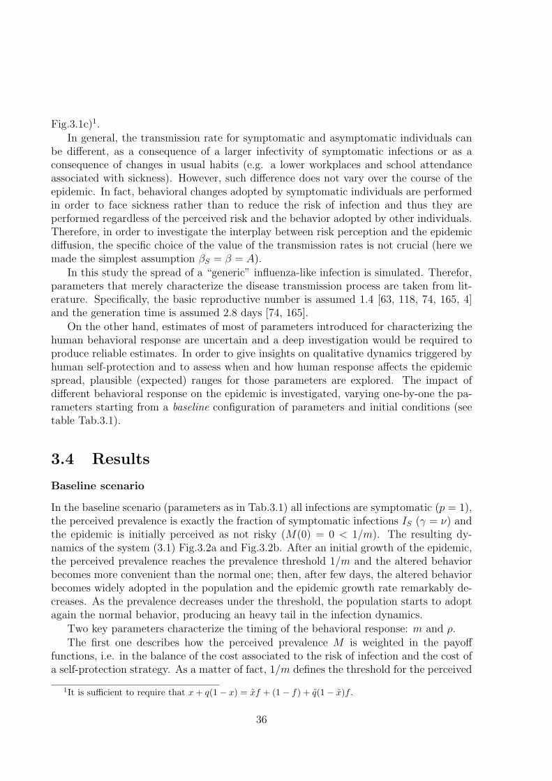
Fig.3.1c)1.

In general, the transmission rate for symptomatic and asymptomatic individuals canbe different, as a consequence of a larger infectivity of symptomatic infections or as aconsequence of changes in usual habits (e.g. a lower workplaces and school attendanceassociated with sickness). However, such difference does not vary over the course of theepidemic. In fact, behavioral changes adopted by symptomatic individuals are performedin order to face sickness rather than to reduce the risk of infection and thus they areperformed regardless of the perceived risk and the behavior adopted by other individuals.Therefore, in order to investigate the interplay between risk perception and the epidemicdiffusion, the specific choice of the value of the transmission rates is not crucial (here wemade the simplest assumption βS = β = A).

In this study the spread of a “generic” influenza-like infection is simulated. Therefor,parameters that merely characterize the disease transmission process are taken from lit-erature. Specifically, the basic reproductive number is assumed 1.4 [63, 118, 74, 165, 4]and the generation time is assumed 2.8 days [74, 165].

On the other hand, estimates of most of parameters introduced for characterizing thehuman behavioral response are uncertain and a deep investigation would be required toproduce reliable estimates. In order to give insights on qualitative dynamics triggered byhuman self-protection and to assess when and how human response affects the epidemicspread, plausible (expected) ranges for those parameters are explored. The impact ofdifferent behavioral response on the epidemic is investigated, varying one-by-one the pa-rameters starting from a baseline configuration of parameters and initial conditions (seetable Tab.3.1).

3.4 Results

Baseline scenario

In the baseline scenario (parameters as in Tab.3.1) all infections are symptomatic (p = 1),the perceived prevalence is exactly the fraction of symptomatic infections IS (γ = ν) andthe epidemic is initially perceived as not risky (M(0) = 0 < 1/m). The resulting dy-namics of the system (3.1) Fig.3.2a and Fig.3.2b. After an initial growth of the epidemic,the perceived prevalence reaches the prevalence threshold 1/m and the altered behaviorbecomes more convenient than the normal one; then, after few days, the altered behaviorbecomes widely adopted in the population and the epidemic growth rate remarkably de-creases. As the prevalence decreases under the threshold, the population starts to adoptagain the normal behavior, producing an heavy tail in the infection dynamics.

Two key parameters characterize the timing of the behavioral response: m and ρ.

The first one describes how the perceived prevalence M is weighted in the payofffunctions, i.e. in the balance of the cost associated to the risk of infection and the cost ofa self-protection strategy. As a matter of fact, 1/m defines the threshold for the perceived

1It is sufficient to require that x+ q(1− x) = xf + (1− f) + q(1− x)f .

36

Days

Dai

ly p

reva

lenc

e of

sym

pt. i

nf.

0 10 20 30 40 50 60 70 80 90 100

110

120

0

0.01

0.02

0.03

0.04

0.054 days

Days

Effe

ct. r

epr.

num

ber

1−x

0 30 60 90 120

0.75

1

1.25

1.5

0

0.25

0.5

0.75

1

Speed of behavioral changes

Imita

tion

dela

y in

day

s

0.26 1 10 100 1000

147

14

21

28

35

Days

Dai

ly p

rev.

of s

ympt

. inf

.

1−x

0 10 20 30 40 50 60 70 80 90 100

110

120

0

0.01

0.02

0.03

0.04

0.05

0

0.5

1a b c d

Figure 3.2: a Daily prevalence of symptomatic infection in the case of no response by thepopulation, q = 1 (bold gray line), and in the baseline scenario, q = 0.85 (bold red line).Other parameters as in the baseline scenario reported in Tab.3.1. The horizontal grayline represents the prevalence threshold 1/m. The behavioral response appears about 4days after the perceived prevalence M(t) = IS(t) crosses the threshold 1/m producing alower increase in the prevalence of infection. b Baseline scenario: the dynamics of 1− x(blue line, scaled on the left) and the effective reproductive number over time (dark greenline, scaled on the right). c Imitation delay as a function of ρ. Other parameters as in thebaseline scenario. For each value of ρ the imitation delay is computed as the time betweenwhen the perceived prevalence crosses the prevalence threshold 1/m and when more than50% of individuals have adopted the altered strategy (x < 0.5). The gray region representsa plausible range for the imitation delay. This, in turn, determines plausible values ofρ. For instance, if ρ = 10 (as assumed in the baseline scenario) the imitation delay is 4days, compliant to that observed in a. d Daily prevalence of symptomatic infection inthe case of no response by the population, q = 1 (bold gray line), and in the baselinescenario, q = 0.85 (bold red line), but for the prevalence threshold 1/m = 10−3. Thisexample shows that, altrough the altered behaviors is (almost) always the most convenientstrategy, human responsiveness takes about 4 days to spread in the population.

prevalence above which individuals reducing contacts have a larger payoff than other ones.The larger is m, the earlier the risk induced by the epidemic is (perceived) sufficientlylarge to make the altered behavior as the most convenient choice.

On the other hand, ρ represents the speed of the imitation process with respect to thedisease transmission time–scale. As a matter of fact, ρ entails the delay (embedded inthe imitation dynamics) between the time at which a strategy becomes more convenientand the time at which the majority of population adopt this strategy. For instance,when 1/m < Is(0), the altered behavior is more convenient than the normal one sincethe beginning of the epidemic. Nonetheless, if x 6= 0, the altered behavior takes sometime to spread in the population as well (see Fig.3.2d). We define the duration of thistransition as the imitation delay. We mesure the imitation delay as the time between

37

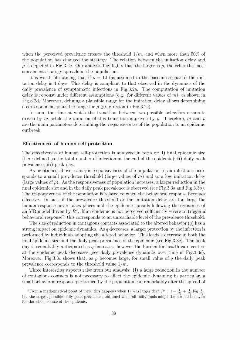
when the perceived prevalence crosses the threshold 1/m, and when more than 50% ofthe population has changed the strategy. The relation between the imitation delay andρ is depicted in Fig.3.2c. Our analysis highlights that the larger is ρ, the erlier the mostconvenient strategy spreads in the population.

It is worth of noticing that if ρ = 10 (as assumed in the baseline scenario) the imi-tation delay is 4 days. This delay is compliant to that observed in the dynamics of thedaily prevalence of symptomatic infections in Fig.3.2a. The computation of imitationdelay is roboust under different assumptions (e.g., for different values of m), as shown inFig.3.2d. Moreover, defining a plausible range for the imitation delay allows determininga correspondent plausible range for ρ (gray region in Fig.3.2c).

In sum, the time at which the transition between two possible behaviors occurs isdriven by m, while the duration of this transition is driven by ρ. Therefore, m and ρare the main parameters determining the responsiveness of the population to an epidemicoutbreak.

Effectiveness of human self-protection

The effectiveness of human self-protection is analyzed in term of: i) final epidemic size(here defined as the total number of infection at the end of the epidemic); ii) daily peakprevalence; iii) peak day.

As mentioned above, a major responsiveness of the population to an infection corre-sponds to a small prevalence threshold (large values of m) and to a low imitation delay(large values of ρ). As the responsiveness of population increases, a larger reduction in thefinal epidemic size and in the daily peak prevalence is observed (see Fig.3.3a and Fig.3.3b).The responsiveness of the population is related to when the behavioral response becomeseffective. In fact, if the prevalence threshold or the imitation delay are too large thehuman response never takes places and the epidemic spreads following the dynamics ofan SIR model driven by Rn

0 . If an epidemic is not perceived sufficiently severe to trigger abehavioral response2, this corresponds to an unreachable level of the prevalence threshold.

The size of reduction in contagious contacts associated to the altered behavior (q) has astrong impact on epidemic dynamics. As q decreases, a larger protection by the infection isperformed by individuals adopting the altered behavior. This leads a decrease in both thefinal epidemic size and the daily peak prevalence of the epidemic (see Fig.3.3c). The peakday is remarkably anticipated as q increases; however the burden for health care centersat the epidemic peak decreases (see daily prevalence dynamics over time in Fig.3.3c).Moreover, Fig.3.3c shows that, as ρ becomes large, for small value of q the daily peakprevalence corresponds to the threshold value 1/m.

Three interesting aspects raise from our analysis: (i) a large reduction in the numberof contagious contacts is not necessary to affect the epidemic dynamics; in particular, asmall behavioral response performed by the population can remarkably alter the spread of

2From a mathematical point of view, this happens when 1/m is larger than Ip = 1− 1Rn

0+ 1

Rn0log 1

Rn0,

i.e. the largest possible daily peak prevalence, obtained when all individuals adopt the normal behaviorfor the whole course of the epidemic.

38

Days

Dai

ly p

reva

lenc

e of

sym

pt. i

nfec

tions 1/m = 0.06

1/m = 0.0241/m = 0.0161/m = 0.0121/m = 0.0081/m = 0.004

0 10 20 30 40 50 60 70 80 90 100

110

120

0

0.01

0.02

0.03

0.04

0.05

Threshold prevalence (1/m)

Fin

al e

pide

mic

siz

e

0

0.01

0.02

0.03

0.04

0.05

0.06

30

35

40

45

50

55

Days

Dai

ly p

reva

lenc

e of

infe

ctio

ns

p = 0.2p = 0.3p = 0.4p = 0.5p = 0.7p = 1

0 10 20 30 40 50 60 70 80 90 100

110

120

0

0.01

0.02

0.03

0.04

0.05

Days

Dai

ly p

reva

lenc

e of

sym

pt. i

nfec

tions q = 1

q = 0.94q = 0.9q = 0.84q = 0.72q = 0.6

0 10 20 30 40 50 60 70 80 90 100

110

120

0

0.01

0.02

0.03

0.04

0.05

Reduction of potentially inf. contacts (q)

Fin

al e

pide

mic

siz

e

0.5

0.6

0.7

0.8

0.9 1

30

35

40

45

50

55

Probability of developing symptoms (p)

Fin

al e

pide

mic

siz

e

0.1

0.25 0.

5

0.75 1

0

10

20

30

40

50

Threshold prevalence (1/m)

Dai

ly p

eak

prev

alen

ce

0

0.01

0.02

0.03

0.04

0.05

0.06

0

0.01

0.02

0.03

0.04

0.05

Threshold prevalence (1/m)P

eak

day

0

0.01

0.02

0.03

0.04

0.05

0.06

20

25

30

35

40

45

50

55

60

Reduction of potentially inf. contacts (q)

Dai

ly p

eak

prev

alen

ce

0.5

0.6

0.7

0.8

0.9 1

0

0.01

0.02

0.03

0.04

0.05

Reduction of potentially inf. contacts (q)

Pea

k da

y

0.5

0.6

0.7

0.8

0.9 1

20

25

30

35

40

45

50

55

60

Probability of developing symptoms (p)

Da

ily p

ea

k p

reva

len

ce

0.1

0.2

5

0.5

0.7

5 1

0

0.01

0.02

0.03

0.04

0.05

Probability of developing symptoms (p)

Pe

ak d

ay

0.1

0.2

5

0.5

0.7

5 1

0

10

20

30

40

50

60

70

Speed of behavioral changes (ρ)

Pea

k da

y

−1 0 1 2 3

20

25

30

35

40

45

50

55

60

Speed of behavioral changes (ρ)

Dai

ly p

eak

prev

alen

ce

−1 0 1 2 3

0

0.01

0.02

0.03

0.04

0.05

Days

Dai

ly p

reva

lenc

e of

sym

pt. i

nfec

tions ρ = 0.017

ρ = 0.56ρ = 1ρ = 3.15ρ = 10ρ = 1000

0 10 20 30 40 50 60 70 80 90 100

110

120

0

0.01

0.02

0.03

0.04

0.05

Speed of behavioral changes (ρ)

Fin

al e

pide

mic

siz

e

−1 0 1 2 3

30

35

40

45

50

55

c) Reduction of potentially infectious contacts d) Probability of developing symptoms

b) Speed of behavioral changesa) Prevalence threshold

a2a1 a3

a4

c2c1 c3

c4

d1 d2 d3

d4

b1 b2 b3

b4

Figure 3.3: a Daily prevalencee of symptomatic infections (a1), final epidemic size (a2),daily peak prevalence of symptomatic infections (a3) and peak day (a4) as obtained fordifferent values of the prevalence threshold 1/m. Other parameters as in the baselinescenario (see Tab.3.1). b As a but for different values of the speed of behavioral changesρ. c As a but for different values of the reduction in potentially infectious contacts q. dAs a but for different values of the probability of developing symptoms p.

the epidemic; (ii) it exists a threshold for q, such that a further increase in the reductionq does not determine a larger impact of behavioral changes on the final epidemic size, thedaily peak prevalence and the peak day; (iii) for small values of q multiple epidemic wavescan occur. Indeed, a reduction of 100% in the number of potentially infectious contacts(corresponding to q = 0, i.e. assuming total isolation) results in a similar final epidemicsize, daily peak prevalence and peak day to that observed by considering a reductionof 25% (q = 0.75). On the other hand, large values of q can trigger multiple epidemicwaves. The conditions for observing multiple epidemic waves has been already discussedin [53, 127]. Briefly, the chance of observing multiple epidemic waves increase as thehuman responsiveness to the epidemic increases, i.e. for large values of ρ or m.

When considering the possibility of asymptomatic infections (p < 1, but still assumingβS = βA), asymptomatic infectives can adopt the altered behavior as well. Since they arenot aware of their infection, they have no reason to behave differently from susceptibles.As the fraction of asymptomatic infections increases (i.e. as p decreases), the fraction ofindividuals adopting a self-protection strategy increases as well. On the other hand, alarger symptomaticity produces a larger number of observable infections and, in turn, a

39

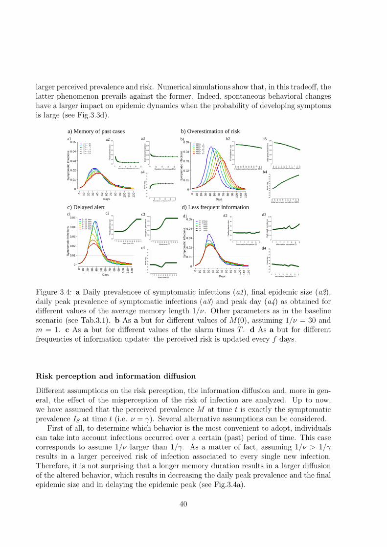
larger perceived prevalence and risk. Numerical simulations show that, in this tradeoff, thelatter phenomenon prevails against the former. Indeed, spontaneous behavioral changeshave a larger impact on epidemic dynamics when the probability of developing symptomsis large (see Fig.3.3d).

Duration of memory (1/µ)

Dai

ly p

eak

prev

alen

ce

0 20 40 60 80

0

0.01

0.02

0.03

0.04

0.05

Duration of memory (1/µ)

Pea

k da

y

0 20 40 60 80 100

20

25

30

35

40

45

50

55

60

Days

Sym

ptom

atic

Infe

ctio

ns

M(0) = 1M(0) = 1.5M(0) = 2M(0) = 2.5M(0) = 3M(0) = 3.5

0 10 20 30 40 50 60 70 80 90 100

110

120

0

0.01

0.02

0.03

0.04

0.05

Initial perceived prevalence (M(0))

Fin

al e

pide

mic

siz

e

0.6

0.9

1.2

1.5

1.8

2.1

2.4

2.7 3

3.3

3.6

30

35

40

45

50

55

Days

Sym

ptom

atic

Infe

ctio

ns

= 36 = 10 = 7 = 5 = 3.4 = 2.81 ν

1 ν1 ν1 ν1 ν1 ν

0 10 20 30 40 50 60 70 80 90 100

110

120

0

0.01

0.02

0.03

0.04

0.05

Duration of memory (1/µ)

Fin

al e

pide

mic

siz

e

0 20 40 60 80 100

30

35

40

45

50

55

Initial perceived prevalence (M(0))

Dai

ly p

eak

prev

alen

ce

0.6

0.9

1.2

1.5

1.8

2.1

2.4

2.7 3

3.3

3.6

0

0.01

0.02

0.03

0.04

0.05

Initial perceived prevalence (M(0))

Pea

k da

y

0.6

0.9

1.2

1.5

1.8

2.1

2.4

2.7 3

3.3

3.6

20

25

30

35

40

45

50

55

60

65

70

Information frequence (f)

Dai

ly p

eak

prev

alen

ce

0 2 4 6 8 10 12 14

0

0.01

0.02

0.03

0.04

0.05

Information frequence (f)

Pea

k da

y

0 2 4 6 8 10 12 14

20

25

30

35

40

45

50

55

60

Days

Sym

ptom

atic

Infe

ctio

ns

f = 14 daysf = 12 daysf = 7 daysf = 3 daysf = 2 daysf = 1 days

0 10 20 30 40 50 60 70 80 90 100

110

120

0

0.01

0.02

0.03

0.04

0.05

Days

Sym

ptom

atic

Infe

ctio

ns

T = 60 daysT = 35 daysT = 30 daysT = 25 daysT = 20 daysT = 10 days

0 10 20 30 40 50 60 70 80 90 100

110

120

0

0.01

0.02

0.03

0.04

0.05

Alert time (T)

Fin

al e

pide

mic

siz

e

1 5 10 15 20 25 30 35 40 45 50 55 60

30

35

40

45

50

55

Alert time (T)

Dai

ly p

eak

prev

alen

ce

1 5 10 15 20 25 30 35 40 45 50 55 60

0

0.01

0.02

0.03

0.04

0.05

Alert time (T)

Pea

k da

y

1 5 10 15 20 25 30 35 40 45 50 55 60

20

25

30

35

40

45

50

55

60

Information frequence (f)

Fin

al e

pide

mic

siz

e

0 2 4 6 8 10 12 14

30

35

40

45

50

55

c) Delayed alert d) Less frequent information

b) Overestimation of riska) Memory of past casesa1 a2 a3

a4

b1 b3

b4

d4

d3d1

c4

c3c2

b2

c1 d2

Figure 3.4: a Daily prevalencee of symptomatic infections (a1), final epidemic size (a2),daily peak prevalence of symptomatic infections (a3) and peak day (a4) as obtained fordifferent values of the average memory length 1/ν. Other parameters as in the baselinescenario (see Tab.3.1). b As a but for different values of M(0), assuming 1/ν = 30 andm = 1. c As a but for different values of the alarm times T . d As a but for differentfrequencies of information update: the perceived risk is updated every f days.

Risk perception and information diffusion

Different assumptions on the risk perception, the information diffusion and, more in gen-eral, the effect of the misperception of the risk of infection are analyzed. Up to now,we have assumed that the perceived prevalence M at time t is exactly the symptomaticprevalence IS at time t (i.e. ν = γ). Several alternative assumptions can be considered.

First of all, to determine which behavior is the most convenient to adopt, individualscan take into account infections occurred over a certain (past) period of time. This casecorresponds to assume 1/ν larger than 1/γ. As a matter of fact, assuming 1/ν > 1/γresults in a larger perceived risk of infection associated to every single new infection.Therefore, it is not surprising that a longer memory duration results in a larger diffusionof the altered behavior, which results in decreasing the daily peak prevalence and the finalepidemic size and in delaying the epidemic peak (see Fig.3.4a).

40

The role of memory becomes more relevant when the population overestimates the riskof infection during the early phases of the epidemic. For instance, such kind of overestima-tion may happen as a consequence of the concern raised after a mass media campaign (ascould have happened during 2009 H1N1 pandemic [90, 136]). An initial overestimation ofthe risk of infection can result an initial perceived risk above the threshold, even when thethreshold is too large for supporting the altered behavior as the most convenient one. Infact, if the number of new cases produced by the epidemic is not sufficient to support thealtered behavior as more convenient, the effect of misperception can vanish. On the otherhand, when the initial misperception of prevalence is supported by a long lasting memorythe altered behavior can result as the most convenient one for a relevant period of time.This essentially results in an initial reduced growth rate of the epidemic, which delays theepidemic (see Fig.3.4b). Moreover, if the initial overestimation of risk is supported for asufficiently large period of time, both the daily peak prevalence and the final epidemicsize decrease as well.

The misperception of risk can also occur when the population becomes aware of a newepidemic outbreak after a certain period of time, since the emergence of the epidemic. Thisphenomenon can be investigated by assuming that the perceived prevalence is initiallyequal to zero for a period of time T . Numerical simulation show that the larger is thedelay T , the lower the effectiveness of human response becomes. In particular, the dailypeak prevalence and the final epidemic size increase as T increases (see Fig.3.4c) and, ifthe alert takes place late in the course of the epidemic no relevant effects on the outbreakcan be detected (see Fig.3.4c).

Finally, regardless of misperceptions or misjudgments of the risk of infection, it is fairyreasonable to assume that individuals may acquire information about the status of theepidemic only once in a while, e.g. f days, rather than in real time3. Our investigationhighlights that less frequent information does not clearly reduce the effectiveness of thebehavioral response of the population, unless very rare information is considered (seeFig.3.4d).

The main results presented in this manuscript are summarized in Fig.3.5. Specifically,we found that, if perceived risk associated to an epidemic is sufficiently large (i.e. forlarge values of m), even small behavioral changes can remarkably reduce the impact ofthe epidemic (e.g. for q = 0.9 the final epidemic size can decrease from about 52% toabout 38%). Moreover, if the imitation delay is not too large (lower than 2 weeks),the response of the population is always effective. On the other hand, the populationresponsiveness increases as the symptomaticity increases, while memory of past cases andan initial overestimation of the risk of infection essentially delay the epidemic spread.

3However, driven by the balance based on the last information acquired by the individuals, behavioralchanges may occur continuously over time.

41

3.5 Discussion

Human response to the perceived risk of infection can remarkably affect the epidemicspread both qualitatively and quantitatively. Nonetheless, human behavior cannot bemerely considered as an independent background process of the infection dynamics. Theintroduced model provides a promising approach, based on evolutionary game theory, toinvestigate the complex interaction between human behavior and diseases transmissionprocess. Moreover, the model is fairy general to be applied for describing any kind ofdisease (e.g. influenza, smallpox, SARS and endemic diseases as well).

This study represents a further step to assess quantitative and qualitative effects ofspontaneous behavioral response to the perceived risk of infection. Key features of ahuman self-protection are captured as well as how and when behavioral responses areeffective. Our results are consistent to those obtained by previous works through differentassumptions. Specifically, as shown in [42], the disease spread results highly sensitive tohow rapidly people adopt a self-reduction in their contact activity rates. Moreover, ifbehavioral changes are fast enough, they can have a remarkable effect in reducing thedaily prevalence of infection [93] and the final epidemic size [67]. For suitable parameterconfigurations, the epidemic dynamics becomes quite rich and can account for multipleepidemic waves, as shown in [53, 127].

Spontaneous behavioral changes have detected to be occurred in recent epidemics.For instance, during the 2009 H1N1 pandemic, high levels of concern have been detectedamong individuals exposed to the infection [90, 136]. Moreover, spontaneous behavioralchanges performed as response to an emerging epidemic have been detected during pastepidemics. On 2003 this was the case of the SARS epidemic when individuals changedtheir behavioral patters in order to reduce their susceptibility to the infection by limitingtravels [98, 59], wearing face masks and performing other self-prophylaxis measures [98].

Therefore, accounting for spontaneous behavioral changes would be helpful for givinginsight to public health policy makers, for planning control strategies and for betterestimating the burden for health care centers over time. However, at the current stage, theproposed model could hardly be used for real time predictions. In fact, a deep investigationon plausible values of model parameters related to human behavior is required. In orderto gain a major consciousness on how such mechanisms work Further investigations maybe devoted to the investigation of real epidemic outbreaks where behavioral changes haveobserved.

42

Table 3.1: Parameters employed and initial conditions

EPIDEMIOLOGICAL PARAMETERS?

Parameter Interpretation Investigation Baselinerange value

1/γ Average length of - 2.8the infectivity period (days)

βS Transmission rate for - 0.5symptomatic individuals (days−1)

βA Transmission rate for - 0.5asymptomatic individuals (days−1)

p Probability of developing [0, 1] 1symptoms

S(0) Initial fraction of - 1− 10−3

susceptible individualsIA(0) Initial fraction of - 0

asymptomatic infective individualsIS(0) Initial fraction of - 10−3

symptomatic infective individualsRA(0) Initial fraction of - 0

asymptomatic recovered individualsRS(0) Initial fraction of - 0

symptomatic recovered individuals

BEHAVIORAL PARAMETERS

Parameter Interpretation Investigation Baselinerange value

q Reduction in the number of [0.5, 1] 0.85potentially infectious contacts

1/m Prevalence threshold/risk [0, 0.05] 0.01ρ Speed of the behavioral [10−1, 103] 10

changes (days−1)1/ν Average memory length [1, 30] 2.8µ Rate of irrational exploration [0, 10−2] 10−8

x(0) Initial fraction of individuals - 1− 10−6

adopting the normal strategyM(0) Initial perceived prevalence [0, 0.05]† 0

? The epidemiological parameter lead to a baseline configuration withgeneration time 2.8 days and basic reproductive number Rn

0 = 1.4(assuming that all individuals adopt the normal behavior).

† The perceived prevalence can also be considered larger when theinitial risk of the epidemic is overestimated.

43

Fin

al e

pide

mic

siz

e

q ρ m p ν M(0) T f

30%

40%

50%

60%

Dai

ly p

eak

prev

alen

ce

q ρ m p ν M(0) T f

0.01

0.02

0.03

0.04

0.05

Pea

k da

y

q ρ m p ν M(0) T f

2030

4050

6070

c

b

a

Figure 3.5: Results summary The influence of different key features of human behav-ioral responses on: a final epidemic size, b daily peak prevalence and c peak day. Differentparameters have been investigated in the ranges defined in Tab.3.1. Colors represent theresponsiveness of the population: warmer colors correspond to higher responsive popula-tion. Gray boxes have been used where no specific patterns were observed. The dashedline represents the baseline scenario, the red line represents a fully not responsive pop-ulation (i.e., it corresponds to a “simple” SIR model driven by Rn

0 ) and the blue linerepresents a fully responsive population (i.e., it corresponds to a “simple” SIR modeldriven by Ra

0.44

Chapter 4

The effect of risk perception on the2009 H1N1 pandemic influenzadyanmics

4.1 Introduction

Among the many factors known to influence the spread of epidemics across human popu-lations, a central role is played by the characteristics of the pathogen responsible for theinfections [6, 19], human mobility patterns [84, 38, 151, 11, 112], the sociodemographicstructure of the population [112] and intervention measures [6, 92]. Changes in humanbehaviors are largely suspected to play a crucial role as well [42, 53, 127, 67, 130]. Asmathematical modeling becomes a powerful tool for decision making both in pre-planning[103, 104, 57, 58, 73, 164, 33, 41, 78, 113] and in real-time situations [12, 75, 4, 99], knowingin advance how to account for spontaneous behavioral changes would greatly improve thepredictive power of epidemic transmission models and the evaluation of the effectivenessof control strategies.

In March 2009 a new influenza virus emerged in Mexico [162]. Early in the course ofthe pandemic the population was very concerned about the event [136, 90]. Did this af-fect the behavior of the population and, consequently, alter the dynamics of the epidemic?By analyzing the 2009-2010 Influenza-Like Illness (ILI) incidence in Italy, as reported tothe national surveillance system, the hypothesis appears plausible that spontaneous be-havioral changes have played a role in the pandemic, contributing to change the timingof spread and the transmissibility potential. In fact, after an initial period (September– mid-October 2009) characterized by a slow exponential increase in the weekly ILI in-cidence, a sudden and sharp increase of the growth rate was observed by mid-October.Over the whole period schools remained open [54] and only moderate mitigation measureswere enacted (e.g., antiviral treatment of severe cases) [86]. However, during the initialphases of the epidemic the Italian population has been exposed to a massive informationcampaign on the risks of an emerging influenza pandemic, which can have contributed toalter the perceived risk. The aim of this study is to investigate the effects of the perceived

45

risk of infection during the course of the 2009 H1N1 pandemic in Italy. In particular,we propose a new modeling framework, based on evolutionary game theory, accountingexplicitly for the dynamics of behavioral patterns adopted across the population.

4.2 Materials and Methods

4.2.1 Data description

In Italy, influenza surveillance system INFLUNET (accessible at: http://www.iss.it/iflu/)is based on a nationwide voluntary sentinel network of general practitioners and pedia-tricians. The aim is to monitor ILI incidence and to collect information on circulatingstrains. Incidence rates are based on the population served by each reporting physicianeach week.

As most European countries, Italy has experienced one single pandemic wave duringfall-winter 2009 and no substantial activity has been detected during the summer [4]. Thepandemic has mainly spread starting since the reopening of schools in mid-Septemberuntil mid-December. During the whole period schools remained open, in fact neitherregular holidays were scheduled [54] nor mitigation strategies were performed, except for amoderate vaccination program started on mid-October, and involving only a small fractionof at-risk patients and essential workers (the fraction of individuals vaccinated during thewhole course of the pandemic is less than 1.5% of the population) and treatment of severecases with antiviral drugs [86]. In this study, we consider total ILI incidence from week38 (corresponding to the reopening of schools after the summer break, when influenzaactivity started to be detected by the surveillance system) to 50, 2009. This allows us toinvestigate an “uncontrolled” epidemic, not affected by heavy public health interventionsor by school closure. The number of practitioners involved in the surveillance systemover the considered period varies from 561 to 1,165; consequently, the served populationvaries from 767,154 and 1,509,971. These values guarantee the reliability of the numberof weekly reported cases.

4.2.2 The model

The transmission process is based on a SIR model where susceptible individuals mayadopt two mutually exclusive behaviors, “normal” and “altered”, on the basis of the per-ceived risk of infection. Individuals adopting altered behavior are supposed to be ableto reduce the risk of infection by reducing the force of infection to which they are ex-posed. This defensive response takes into account both reduction in physical contactsand, more in general, all self-prophylaxis measures which can reduce the transmissionprobability during these contacts. For instance, a self reduction in the number of con-tacts can occur through the avoidance of crowded environments or by limiting travels,whereas a reduction in transmission probability can be achieved by increasing wariness inusual activities involving other individuals (e.g., the behavioral goals recommended by the

46

WHO for reducing influenza transmission, such as washing hands frequently or respectingcough/respiratory etiquette [161]).

In the model, individuals can change their behavior spontaneously, on the basis ofcost/benefit considerations. This phenomenon perfectly fits to the language of evolu-tionary game theory, in which behaviors adopted by individuals correspond to strategiesplayed in a suitable game, with certain expected payoffs: altered behavior takes the advan-tage of reducing the risk of infection, but it is more costly (e.g., because individuals haveto limit their activities). Which behavior is more convenient to adopt clearly depends onthe state of the epidemic. The balance of the payoff between the two possible behaviorsis determined by the perceived risk of infection, which depends on the cost associated tothe risk of infection and on the perceived prevalence of infections in the population. Thelatter is modeled by assuming a fading memory mechanism (such in [48, 3]) altering theperception of the risk of infection on the basis of the number of cases occurred over acertain (past) period of time. The diffusion of strategies in the population is modeled asan imitation process [81, 15] based on the idea that individuals change strategy as theybecome aware that their payoff can increase by adopting another behavior. Denoting byS, I, R the fraction of susceptible, infective and recovered individuals respectively andby introducing the variables x, describing the fraction of individuals adopting normalbehavior, and M , describing the perceived prevalence of infection in the population, thesystem of ordinary differential equations regulating this process can be written as follows:

S = −βIS [x+ q(1− x)]

I = βIS [x+ q(1− x)]− γI

R = γI

M = βIS [x+ q(1− x)]− θMx = x(1− x)(q − 1)βI + ρx(1− x)(1−mM)S

where β is the transmission rate; 1/γ is the average duration of infectivity period (cor-responding to the generation time); q represents the reduction of the risk of infectionto which individuals adopting altered behavior are exposed; θ weighs the decay of theperceived prevalence; ρ essentially represents the speed of the imitation process with re-spect to the pathogen transmission dynamics; m defines the risk threshold for determiningwhich behavior would represent the most convenient choice.

Briefly, the last equation of the system models the diffusion of the two different be-haviors in the population driven by an imitation/natural selection process. The first termof the equation accounts for a natural selection embedded into the transmission processthat favors individuals reducing the risk of infection, while the second one accounts for animitation process modeling spontaneous changes in individual behaviors. These changesoccur on the basis of the difference between the payoffs of the two possible behaviors,the perceived prevalence, the level of the risk threshold and the speed of the imitationprocess which, in general, is different from the speed of the disease transmission process(as imitation is based on the diffusion of information rather than on physical contactsbetween individuals). Model details are presented in the Supporting Text 8.2.

47

The basic reproductive number R0, which is essentially the average number of sec-ondary infections that results from a single infectious individual in a fully susceptiblepopulation [6], can be computed by using next generation technique [44]. The result-

ing basic reproductive number is R0 =β

γ[x+ q(1− x)], which can be interpreted as a

weighted sum of two basic reproductive numbers: Rn0 =

β

γ, the reproductive number

for individuals adopting the normal behavior (namely the fraction x) and Ra0 = q

β

γ, the

reproductive number for individuals adopting the altered behavior (namely the fraction1 − x). Therefore, R0 depends on the fraction of individuals in the population who arecurrently adopting either normal or altered behavior.

4.3 Results

The ILI incidence as reported to the surveillance system during the 2009 H1N1 pandemicshows two different phases characterized by two distinct exponential growth rates, es-pecially appreciable when data are plotted in a logarithmic scale (see Fig. 1a and itssub-panel). The “classical” SIR model is not able to catch this phenomenon (see Fig. 1b)unless by considering a time-dependent transmission rate, switching from a low transmis-sion level during the first four weeks to a higher level for the rest of the epidemic (see Fig.1c). However, this model is not able to explain the motivation underlying this suddenchange in the transmissibility potential.

On the contrary, the model introduced here perfectly fits the observed ILI incidence(see Fig. 1a) providing a plausible explanation of the mechanisms responsible for theobserved pattern. Specifically, the estimated parameter configuration obtained by fittingILI incidence entails an initial overestimation of the perceived risk that decreases overtime, along with an initial diffusion of the altered behavior in the population which be-comes replaced by the normal behavior during the course of the epidemic. In fact, a highlevel of perceived risk of infection at the beginning of the pandemic leads the simulatedpopulation to adopt the altered behavior (as in the presence of a well sustained circulationof the virus) resulting in a growth rate of the epidemic lower than what would have beenobserved in a population adopting the normal behavior. Along with a slow increase inthe number of cases, a decrease in the perceived risk of infection is observed. In fact, thelatter depends on the combination of these two opposite phenomena: the increase of newinfections and the decline of the perceived prevalence (slowed by the memory mechanism),which was overestimated in the early phases of the epidemic. As the perceived prevalencegoes below the risk threshold 1/m, the normal behavior starts to spread quickly in thepopulation as the most convenient strategy to be adopted through the subsequent courseof the epidemic. This induces an increase of R0 which leads to a sudden change in thegrowth rate of the epidemic. Thus, these two distinct exponential growth phases in theobserved ILI incidence correspond to two phases in the model: the first one characterizedby the diffusion of the altered behavior in the population and thus driven by Ra

0, and the

48

Weeks (week of the year)

Wee

kly

inci

denc

e (c

ases

per

1,0

00 in

divi

dual

s)

38 39 40 41 42 43 44 45 46 47 48 49 50 51

0

4

8

12

16

log

scal

e

38 40 42 44 46 48 50

−3

−1.5

0

1.5

3a

Weeks (week of the year)

Wee

kly

inci

denc

e (c

ases

per

1,0

00 in

divi

dual

s)

38 39 40 41 42 43 44 45 46 47 48 49 50 51

0

4

8

12

16

log

scal

e

38 40 42 44 46 48 50

−3

−1.5

0

1.5

3

Weeks (week of the year)

Wee

kly

inci

denc

e (c

ases

per

1,0

00 in

divi

dual

s)

38 39 40 41 42 43 44 45 46 47 48 49 50 51

0

4

8

12

16

b c

log

scal

e

38 40 42 44 46 48 50

−3

−1.5

0

1.5

3

Figure 4.1: Comparing observed ILI incidence and model simulations. a WeeklyILI incidence as reported to the surveillance system (green) and weekly incidence sim-ulated by the model (red). Sub-panel shows the same curves in a logarithmic scale.Parameter values used in the simulation are set as follows. The generation time 1/γis assumed 2.5 days according to [63, 165, 74] (a sensitivity analysis on the length ofthe generation time is presented in the Supporting Text 8.2); S(0) = 0.9 according to aserological survey on the Italian population [134]; x(0) = 10−8, assumed; M(0) = 10.5,I(0) = 0.001243, ρ = 66, q = 0.84, m = 0.1, ν = 0.005, β = 0.59, fitted; the estimatedunderreporting factor is 16.9%, in good agreement with the range 18%-20.2% previouslyestimated in [4]. b Weekly ILI incidence as reported to the surveillance system (green)and weekly incidence simulated by a “simple” SIR model (blue). Sub-panel shows thesame curves in a logarithmic scale. Parameter values used in the simulation are set asfollows. The generation time 1/γ is assumed 2.5 days; S(0) = 0.9 according to [134];I(0) = 0.000176, β = 0.58, fitted; the estimated underreporting factor is 17.4%. c WeeklyILI incidence as reported to the surveillance system (green) and weekly incidence sim-ulated by a SIR model assuming a time-dependent transmission rate (blue). Sub-panelshows the same curves in a logarithmic scale. Parameter values used in the simulationare set as follows. The generation time 1/γ is assumed 2.5 days; S(0) = 0.9 accordingto [134]; I(0) = 0.00126, β(t) = 0.496 for weeks 38-41.58 and β(t) = 0.596 for weeks41.58-51, fitted; the estimated underreporting factor is 16.7%.

second one characterized by the diffusion of the normal behavior and thus driven by Rn0 .

The best estimate for Ra0 is 1.24 and for Rn

0 is 1.48 (which correspond to two effectivereproductive numbers of 1.12 and 1.33 respectively, given a 10% initial natural immunityto the 2009 H1N1pdm strain in the Italian population [134]). The basic reproductivenumber estimated in the phase of the epidemic characterized by the normal behavior,namely Rn

0 , is in good agreement with the estimates previously obtained for the 2009pandemic in Italy [4] and in several regions of the world [63, 118, 165, 74, 10].

The analysis of the sensibility of the model to changes in parameter values highlightsthat the model complies with observed ILI incidence only if an initial (persistent) diffusionof the altered behavior in the population is considered (see Supporting Text 8.2). Specifi-cally, an initial perceived risk of infection above the risk threshold, a long-lasting memory

49

mechanism (able to maintain the altered behavior as more convenient over a relevant pe-riod of time) and a fast imitation process (enough to produce a sudden change in theforce of infection) are required. Moreover, model predictions are robust in terms of finalepidemic size (with absolute differences of the order of 3%), while they are more sensiblein terms of timing of the epidemic. Specifically, small variations in the reduction of therisk of infection in individuals adopting the altered behavior result in changing Ra

0 andthus the timing of the epidemic. The same holds if the initial perceived prevalence and therisk threshold determining which behavior is more convenient to adopt are perturbed. Onthe other hand, no relevant differences appear by increasing either the average duration ofthe perceived risk of infection (i.e., the length of the long-lasting memory mechanism) orthe speed of the imitation process. A further analysis (shown in the Supporting Text 8.2)has revealed that, if the risk of infection is overestimated during the early phases of theepidemic, the diffusion of the virus would be slowed down (thus gaining time for vaccineproduction). On the other hand, if such overestimation occurs during the outbreak, alower peak incidence (and thus a lower burden for health care centers) and a relevantdecline of the final epidemic size would be observed.

Results reported above support the hypothesis that the mass media campaign on therisks of an emerging influenza pandemic performed in the early phases of the epidemicmight have induced a high perceived risk of infection at the beginning of the pandemic, asit has been highlighted by specific survey studies [136, 90]. In order to investigate if suchphenomenon could have been a peculiarity of the 2009 pandemic, we also analyzed thelast three influenza seasons in Italy. Our analysis, reported in the Supporting Text 8.2,reveals that during the 2006-2007, 2007-2008 and 2008-2009 influenza seasons behavioralchanges would not have played a relevant role in the early phases of the epidemics.

Beyond the previous analysis, the hypothesis of an overestimation of the risk is sup-ported by the temporal pattern of drug purchases and by sporadic self-imposed schoolclosures. Specifically, during the 2008-2009 influenza season the maximum weekly numberof antiviral drugs sold was under 2 doses per 100, 000 individuals per week, while whenthe 2009 pandemic arrived in Europe (end of April) antiviral drug purchases immediatelyjumped to more than 12 doses per 100, 000 individuals per week [85]. Despite no substan-tial ILI activity has been detected in Italy during the summer, the purchase of antiviraldrugs reached a peak of about 35 doses per 100,000 individuals per week at the end ofJuly. As shown in Fig. 2a and 2b, during fall the purchase of antiviral drugs complies withthe observed ILI temporal dynamics, while until mid-October an excess of antiviral drugpurchase can be observed, supporting the hypothesis of an initial overestimation of therisk of infection. On the contrary, the sales of pain killers (which are commonly used torelieve pain due to mild symptoms) have followed a completely different pattern: duringthe summer the sales have been (nearly) constant, then they started to increase from themiddle of September [85]. The purchase of antiviral drugs might have been amplified bythe concern about the pandemic possibly thanks to the information campaign about theuse of antivirals for treating H1N1 infections. Moreover, from the end of September to thebeginning of October, a few examples of reactive school closure have been documented[94, 97, 96, 95]. Such school closures were “self-imposed” by the scholastic board or sug-

50

Weeks (week of the year)

Exc

ess

of p

urch

ase

of a

ntiv

irals

dru

gs(d

rugs

per

100

,000

indi

vidu

als)

Per

ceiv

ed p

reva

lenc

e (M

(t))

36 37 38 39 40 41 42 43 44 45 46 47 48 49 50 51

−10

−5

0

5

10

15

20

25

30

7

8

9

10

11

12

13

Weeks (week of the year)

We

ekl

y p

urc

ha

se a

ntiv

ira

l dru

gs

(dru

gs

pe

r 1

00

,00

0 in

div

idu

als

)

We

ekl

y IL

I in

cid

en

ce(c

ase

s p

er

1,0

00

ind

ivid

ua

ls)

36

37

38

39

40

41

42

43

44

45

46

47

48

49

50

51

0

10

20

30

40

50

0

2.75

5.5

8.25

11.

13.75

Weeks (week of the year)

Rep

ortin

g fa

ctor

(%

)

38 39 40 41 42 43 44 45 46 47 48 49 50 51

0

20

40

60

80

100

120

140

160ca b

Figure 4.2: Risk perception, antivirals purchase and reporting factor. a Weeklypurchase of antiviral drugs (light blue, scale on the left axis) and weekly ILI incidenceas reported to the surveillance system (green, scale on the right axis) during the 2009-2010 pandemic in Italy. b Light blue points (scale on the left axis) represent the weeklyexcess of the purchase of antiviral drugs. The latter is defined as the difference betweenthe actual and the expected amount of antiviral drugs purchased (which is assumed to beproportional to ILI incidence, and the proportionality constant is computed as the numberof antivirals purchased divided by the ILI incidence averaged over weeks 43-51, i.e. inthe period of sustained transmission). Light blue line represents the best linear modelfit to the excess of purchased antivirals. Horizontal black line represents the thresholdover which the number of antivirals purchased is larger than the expected one. Grey arearepresents the maximum and the minimum excess of antiviral drugs purchased over theweeks 43-51. Red points (scale on the right axis) represent the perceived prevalence ofinfection simulated by the model parameterized as in Fig. 1a. c Weekly reporting factorestimates that enable the simple SIR model (parameters as in Fig. 1b) to exactly fit thereported ILI incidence. The horizontal grey line represents the average reporting factoras computed over the weeks 42-50.

gested by local authorities (at municipality level). However, these sporadic closures canhardly be thought as the only responsible for the low transmission observed during theearly phases of the epidemic. These two examples, however, provide empirical evidencethat a high risk for the ongoing pandemic influenza has been perceived by the Italianpopulation and that individuals have actively performed spontaneous defensive responsemeasures aimed to reduce the risk of infection.

Behavioral changes, though not directly affecting the transmission process, can also berelevant from an epidemiological perspective. For example, as well known by epidemiolo-gists, a high perceived risk during an epidemic can increase the notification rate, especiallyif the surveillance system is based on consultations. However, such phenomenon does notseem to be able to explain (alone) the observed pattern. In fact, a simple SIR model, witha time dependent reporting factor, can capture ILI incidence during the initial phase ofH1N1 pandemic only by considering extremely large values of the reporting factor (evenabove 100%, see Fig. 2c). Similar results have been obtained by investigating a datasetcombining results from the virological and epidemiological surveillance systems which al-lowed the estimation of a theoretic lower bound of the number of H1N1pdm infections in

51

Italy (see in Supporting Text 8.2).

Weeks (week of the year)

Wee

kly

inci

denc

e(c

ases

per

1,0

00 in

divi

dual

s)

38 39 40 41 42 43 44 45 46 47 48 49 50 51

0

4

8

12

16 4 weeks

Figure 4.3: The impact of risk perception. Weekly ILI incidence as reported to thesurveillance system (green) and incidence simulated by the model (red; parameter valuesas in Fig 1a). Weekly incidence simulated by the “classical” SIR model (blue; parametervalues as in Fig. 1b but for I(0) = 0.001243).

As a matter of fact, if changes in human behavioral patterns (such as self-protection)are not taken into account, two opposite outcomes can be observed. Firstly, estimates ofthe growth rate based on the observations during the early phases of the epidemic may leadto an underestimation of the transmissibility potential of the disease and thus to underratethe impact of the epidemic. Secondly, predictions based on robust available estimates ofthe reproductive number (e.g., taken from the analysis in countries where the epidemic isalready well sustained) would lead to overestimate the growth rate of the epidemic duringits early phases, resulting in turn in predicting a faster spread than the actual one. Forinstance, by using a SIR model, accounting for the best parameter estimates as obtainedby fitting the entire epidemic but initializing the system with the actual number of casesat the beginning of autumn 2009 (namely on week 38), the simulations reach the epidemicpeak four weeks in advance with respect to the actual pandemic (see Fig. 3). A similarresult has been observed also in [4], where - using a model not accounting for behavioral

52

changes in the population - the epidemic peak has been predicted two weeks in advancewith respect to the actual value.

4.4 Discussion

A high level of the perceived risk at the beginning of the 2009-10 pandemic is largelysuspected, as well as its effect in slowing the epidemic spread. Our aim here is to validatethis hypothesis by showing that spontaneous behavioral changes in the population mighthave played a central role in the early phases of the pandemic in Italy. Specifically, ILIincidence shows a low (though exponential) growth, followed by a sudden change in itsgrowth rate starting from week 42. Such pattern can hardly be captured by classicalmodels. On the contrary, the proposed approach is able to reproduce it by explicitlymodeling spontaneous behavioral changes in the population. Our analysis is supportedby some empirical evidence (e.g., the purchase of antiviral drugs) and reveals that a highperceived initial risk of infection could be a plausible explanation for such phenomenon.

This study represents a first step for the estimation of the quantitative and qualitativeeffects of spontaneous behavioral changes in the population on the spread of epidemics. Webelieve it provides a promising approach, based on evolutionary game theory, for includingthe behavior dynamics into epidemic transmission models. The proposed approach isgeneral enough to be used for describing any kind of disease where spontaneous behavioralchanges could play a relevant role. Similar approaches have been previously used toinvestigate individual choices in non-compulsory vaccination programs [48, 15, 17, 69, 108].

As shown in this study, behavioral changes (e.g. induced by mass media informa-tion campaigns) can significantly affect the epidemic spread both qualitatively (e.g., byaltering the epidemic dynamics) and quantitatively (e.g., by substantially slowing theepidemic spread or by determining different final epidemic sizes). Therefore, consideringan approach accounting for spontaneous behavioral changes would be helpful for givinginsight to public health policy makers, for planning public health control strategies (e.g.,vaccination) and better estimating the burden for health care centers over time. Moreover,this study highlights that the estimation of fundamental epidemiological parameters (andin particular the reproductive number) could be largely affected by human behaviors.

At the current stage, the proposed model could hardly be used for real time predictionssince our knowledge on plausible values of model parameters related to human behavioris only preliminary. Further investigations on the 2009-2010 pandemic dynamics in othercountries or on other epidemics where behavioral changes have been suspected (e.g., the2002-03 SARS outbreak) have to be performed in order to gain a major consciousness onhow such mechanisms work.

53

54

Chapter 5

Optimal vaccination choice, (static)vaccination games, and rationalexemption

5.1 Introduction

Despite the fundamental role played in history by vaccines, second only to potable waterin the reduction of mortality and morbidity, various forms of exemption to vaccination(conscientious, religious, philosophical) have always been documented [139]. In morerecent times episodes of decline in vaccine uptake have been associated to vaccine scares,e.g. the cases of the whole-cell pertussis vaccine [70], of thimerosal and HBV vaccine [107],up to the MMR scare [64, 142, 163]. In such cases a significant role of anti-vaccinatorsmovements in raising and spreading concerns about vaccine safety was also documented[70, 126].

Today, developed countries are increasingly facing the challenge of rational exemption(RE). By RE we mean, in regimes of voluntary vaccination, the parents decision not toimmunize children after a seemingly rational comparison between the perceived utility ofvaccination, i.e. protection from the risk of infection perceived as very low as a conse-quence of the high herd immunity due to decades of successful vaccination policies - withits disutility, i.e. the risk of vaccine associated side effects. RE is often considered as aform of free riding [145]. Such a behavior, resulting from the optimization performed byrational agents, might well turn out to be myopically rational, since it considers only thecurrent perceived risk of disease, and not the risk of its future resurgence due to decliningcoverage. Some evidence of rational exemption behavior is documented by surveys ofvaccination lifestyles [8, 107, 163, 64].

Theoretical papers based on traditional epidemiological models have investigated theimplications of RE for the dynamics and control of vaccine preventable diseases [72, 48, 49].This literature, which has pointed out the critical interplay between information andvaccinating as well as other disease-related behavior [45], has shown that RE might makeelimination a mission impossible unless the fraction of those who practice RE is small, i.e.

55

below the susceptibility threshold ensuring endemic persistence. Moreover it has shownthat if the information set used by individuals includes past information then the diseasedynamics might yield epidemic waves with very long period. The negative implicationsfor rubella control of a free vaccines market have also been investigated by more realisticepidemiological models [155].

These results call for explanations of vaccination choices by behavioral variables, e.g.economic and psychological, typically neglected in epidemiological models [56]. Besidessome old pioneering work [23, 61], a series of recent intriguing works by Bauch and cowork-ers have attempted to explain RE in its most appropriate framework, i.e. game theory[16, 15, 36, 131]. These papers have provided the first game-theoretic proof of the elim-ination impossible result, and various dynamic implications of RE. These implicationssuggest potential difficulties, both at the national and international level, for global erad-ication plans [13, 55]. In [124] it was suggested that elimination might become possiblewhen more realistic contact network structures including local information are considered.Various applications to influenza control by vaccination, e.g. the role of adaptive behavior[150], and the interplay between perceived and real costs in vaccination choices [69], havealso been considered. A two-population epidemic game related to that studied here wasanalyzed in [129].

In this paper we discuss RE in developed countries by simple static models of voluntaryvaccination behavior. In this case the actual coverage p is the sum of the vaccinationchoices of the individual families. Families make their choices rationally, by minimizinga loss function taking into account both the perceived risk of infection and the perceivedrisk of vaccine associated side effects (VSE).

We first consider the simple optimization problem where homogeneous representativefamilies make their choice without taking into account other families’ choices. We dis-tinguish two cases, i.e. informed families who know the principle of herd immunity, andnot-fully informed ones, who believe that 100% coverage is necessary to avoid any riskof infection. We prove that the elimination impossible result arises as soon as informedfamilies perceive any, however small, cost of VSE. From the case of not-fully informedfamilies we give a possible answer on how patterns of universal vaccination might emerge.This seems to be more likely when lack of knowledge on herd immunity concur with lowperceived costs of VSE.

Next we model vaccination choices as a game where families interact strategically byincorporating the other family choices in their loss function [110, 140]. We assume, asin the theoretical paper [36], the coexistence of two groups of social actors (labeled aspro- and anti-vaccinators) having widely different perceived costs of infection and of VSE.This is broadly consistent with the current situation of developed countries.

Unlike [16] where only the Nash equilibrium in a simultaneous game was considered,we discuss the implications of all the three classical types of agents’ interaction, i.e. alsothe cases of non-simultaneous (Stackelberg) and social planner games [110]. In the Nashcase agents play simultaneously, and take each other’s action as given. In the Stackelberg(or sequential) case, a few active agents lead the game. This seems to be the case ofanti-vaccination groups which appear to be very active in the acquisition of information,

56

and optimize their action by taking into account pro-vaccinators actions [8]. In the socialplanner case a Deus ex machina (social planner) seeks an agreed solution between thetwo groups by minimizing a social loss function given by an average of the two groups’loss functions. We prove that under informed families, the elimination impossible resultcontinues to hold in both Nash and Stackelberg cases. The only case where eliminationis feasible occurs when pro-vaccinators do not perceive any cost from vaccine side effects,and moreover their group is large enough to allow elimination even if the other group doesnot vaccinate at all. In particular the Stackelberg case with anti-vaccinators leadershipalways leads to a lower coverage compared to Nash behavior. Finally, we show that evenin the social planner case elimination is possible only when, provided the pro-vaccinationgroup is large enough, the social planner assigns to anti-vaccinators preferences the 100%of the weight in the social loss function. This allows a nice interpretation of the currentItalian situation.

The paper is organized as follows. Section 2 deals with the basic model of vaccinationchoice. Section 3 discusses models of strategic interaction. Concluding remarks follow.

5.2 A simple model of optimal family behavior with-

out strategic interaction

We consider a common Susceptible-Infective-Removed (SIR) vaccine preventable infec-tion, such as measles or mumps, in a stationary homogeneously mixing population [5].Infection can give rise to serious but non-fatal sequelae. The vaccine is perfect, i.e. pro-viding 100% effective lifelong immunity. Vaccination is voluntary, and it is administeredat birth. No recuperation strategy, such as vaccination at a later date during epochs ofhigher perceived risk, is allowed [48]. The infection is characterized by a basic reproduc-tion number R0 > 1 [5]. This ensures endemic circulation as far as the vaccine uptake isbelow the critical threshold pc = 1− 1/R0 allowing disease elimination [5].

In this section we assume that families behave non-strategically (i.e. we rule outany game-theoretic consideration). Families are fully homogeneous in their preferencestoward vaccination, i.e. we consider a single representative family [110]. This impliesidentical individual decisions, which in turn straightforwardly imply the equality betweenthe individual propensity to vaccinate p and the collective coverage. Real world familieshave only two options: to vaccinate or not their children at birth. In our formulationeach family determines its optimal propensity to vaccinate p, i.e. its vaccine demand, asthe quantity that minimizes its loss function L. The propensity to vaccinate representsthe agent’s probability (i.e. 0 ≤ p ≤ 1) to take the decision to vaccinate. The lossfunction summarizes the cost families will suffer as a consequence of their decisions. Asloss function we take a quadratic additive function, which is the commonest type of lossfunction in economics [110], increasing in the perceived risk of infection ρI(p), and in theperceived risk of vaccine associated side effect ρV (p):

(5.1) L = ρ2I(p) + βρ2V (p)

57

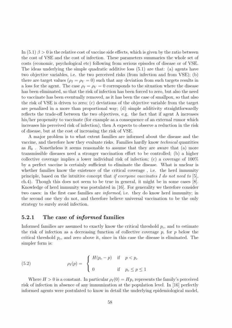
In (5.1) β > 0 is the relative cost of vaccine side effects, which is given by the ratio betweenthe cost of VSE and the cost of infection. These parameters summaries the whole set ofcosts (economic, psychological etc) following from serious episodes of disease or of VSE.The ideas underlying the simple quadratic additive loss (5.1) are that: (a) agents havetwo objective variables, i.e. the two perceived risks (from infection and from VSE); (b)there are target values (ρI = ρV = 0) such that any deviation from such targets results ina loss for the agent. The case ρI = ρV = 0 corresponds to the situation where the diseasehas been eliminated, so that the risk of infection has been forced to zero, but also the needto vaccinate has been eventually removed, as it has been the case of smallpox, so that alsothe risk of VSE is driven to zero; (c) deviations of the objective variable from the targetare penalized in a more than proportional way; (d) simple additivity straightforwardlyreflects the trade-off between the two objectives, e.g. the fact that if agent A increaseshis/her propensity to vaccinate (for example as a consequence of an external rumor whichincreases his perceived risk of infection), then A expects to observe a reduction in the riskof disease, but at the cost of increasing the risk of VSE.

A major problem is to what extent families are informed about the disease and thevaccine, and therefore how they evaluate risks. Families hardly know technical quantitiesas R0 . Nonetheless it seems reasonable to assume that they are aware that (a) moretransmissible diseases need a stronger vaccination effort to be controlled; (b) a highercollective coverage implies a lower individual risk of infection; (c) a coverage of 100%by a perfect vaccine is certainly sufficient to eliminate the disease. What is unclear iswhether families know the existence of the critical coverage , i.e. the herd immunityprinciple, based on the intuitive concept that if everyone vaccinates I do not need to [5],ch.4). Though this does not seem to be true in general, it might be in some cases [8].Knowledge of herd immunity was postulated in [16]. For generality we therefore considertwo cases: in the first case families are informed, i.e. they do know herd immunity; inthe second one they do not, and therefore believe universal vaccination to be the onlystrategy to surely avoid infection.

5.2.1 The case of informed families

Informed families are assumed to exactly know the critical threshold pc, and to estimatethe risk of infection as a decreasing function of collective coverage p, for p below thecritical threshold pc, and zero above it, since in this case the disease is eliminated. Thesimpler form is:

ρI(p) =

H(pc − p) if p < pc

0 if pc ≤ p ≤ 1(5.2)

WhereH > 0 is a constant. In particular ρI(0) = Hpc represents the family’s perceivedrisk of infection in absence of any immunization at the population level. In [16] perfectlyinformed agents were postulated to know in detail the underlying epidemiological model,

58

in particular the functional form π(p) = (pc−p)/(1−p) of the lifetime risk of infection atequilibrium, and to estimate ρI(p) by π(p). This choice and ours are qualitatively equiv-alent (both predict a vanishing risk of infection for p = pc), but ours has the advantage ofbeing simpler, and also less demanding in terms of abstraction. Though (5.2) is formallyequivalent to the equilibrium force of infection in the SIR model [5], we prefer to interpret(5.2) as a coarse qualitative estimate of the lifetime risk of infection, consistently with theabove made assumption that agents do not know technical quantities,.

The perceived risk ρV of a VSE is modeled as the product αp of the family propensityp to vaccinate children, times the conditional probability α > 0 (exogenously given)of suffering a side effect given vaccination relative to the corresponding probability ofsuffering serious disease following infection.

The informed representative family aims therefore at choosing the value of p whichminimizes the loss function 1:

L(p) =

H2(pc − p)2 + βα2p2 if p < pc

βα2p2 if p ≥ pc

(5.3)

Note that L(p) has a continuous first derivative. The idea underlying the quadraticloss, as (5.3), is that families perceive two type of costs, one arising from the risk ofinfection, the other one from the risk of VSE, and want make both them as low aspossible. In [16] the expected loss L(p) = ρI(p)(1− p) + βρV (p) was used

2.

Note first that if β = 0, i.e. if no cost is perceived from VSE, then (5.3) becomes:

L(p) =

H2(pc − p)2 if p < pc

0 if p ≥ pc

(5.4)

One immediately notes that for p < pc, the graph of L(p) is an arc of paraboladecreasing to zero as p tends to pc, implying that any choice p equal to, or above thecritical coverage pc is optimal for the individual. In other words if no costs arise fromVSE it is optimal for the individual to achieve the elimination threshold.

For β > 0 the loss function is decreasing for small p and increasing for p ≥ pc, implyingthat the optimal solution can never exceed pc. This means that policies in excess ofthe critical level are more costly also at the individual level, as they expose people to

1More general results can be obtained by more general formulations allowing interpolation betweenthe linear and quadratic loss formulations, as suggested by an anonymous referee for these suggestions.

2It is possible to see that eventually the two formulations yield the same conclusions. The onlydifference is that the expected loss allows a dichotomy result, i.e. no one will vaccinate if the cost of VSEis always higher than the cost of infection, while in the opposite case some will vaccinate. Though theformer case is of theoretical interest as it yields a no vaccination equilibrium, it does not seem to havepractical relevance.

59

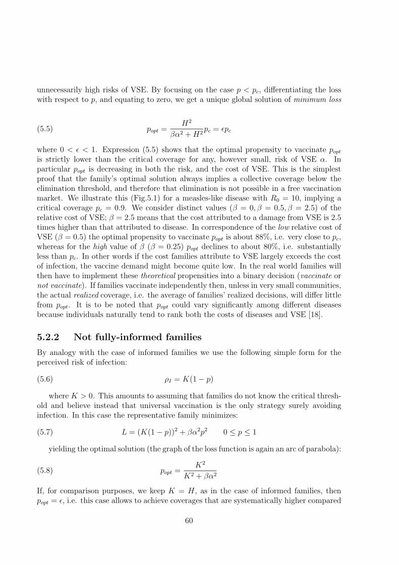
unnecessarily high risks of VSE. By focusing on the case p < pc, differentiating the losswith respect to p, and equating to zero, we get a unique global solution of minimum loss

(5.5) popt =H2

βα2 +H2pc = εpc

where 0 < ε < 1. Expression (5.5) shows that the optimal propensity to vaccinate poptis strictly lower than the critical coverage for any, however small, risk of VSE α. Inparticular popt is decreasing in both the risk, and the cost of VSE. This is the simplestproof that the family’s optimal solution always implies a collective coverage below theelimination threshold, and therefore that elimination is not possible in a free vaccinationmarket. We illustrate this (Fig.5.1) for a measles-like disease with R0 = 10, implying acritical coverage pc = 0.9. We consider distinct values (β = 0, β = 0.5, β = 2.5) of therelative cost of VSE; β = 2.5 means that the cost attributed to a damage from VSE is 2.5times higher than that attributed to disease. In correspondence of the low relative cost ofVSE (β = 0.5) the optimal propensity to vaccinate popt is about 88%, i.e. very close to pc,whereas for the high value of β (β = 0.25) popt declines to about 80%, i.e. substantiallyless than pc. In other words if the cost families attribute to VSE largely exceeds the costof infection, the vaccine demand might become quite low. In the real world families willthen have to implement these theoretical propensities into a binary decision (vaccinate ornot vaccinate). If families vaccinate independently then, unless in very small communities,the actual realized coverage, i.e. the average of families’ realized decisions, will differ littlefrom popt. It is to be noted that popt could vary significantly among different diseasesbecause individuals naturally tend to rank both the costs of diseases and VSE [18].

5.2.2 Not fully-informed families

By analogy with the case of informed families we use the following simple form for theperceived risk of infection:

(5.6) ρI = K(1− p)

where K > 0. This amounts to assuming that families do not know the critical thresh-old and believe instead that universal vaccination is the only strategy surely avoidinginfection. In this case the representative family minimizes:

(5.7) L = (K(1− p))2 + βα2p2 0 ≤ p ≤ 1

yielding the optimal solution (the graph of the loss function is again an arc of parabola):

(5.8) popt =K2

K2 + βα2

If, for comparison purposes, we keep K = H, as in the case of informed families, thenpopt = ε, i.e. this case allows to achieve coverages that are systematically higher compared

60

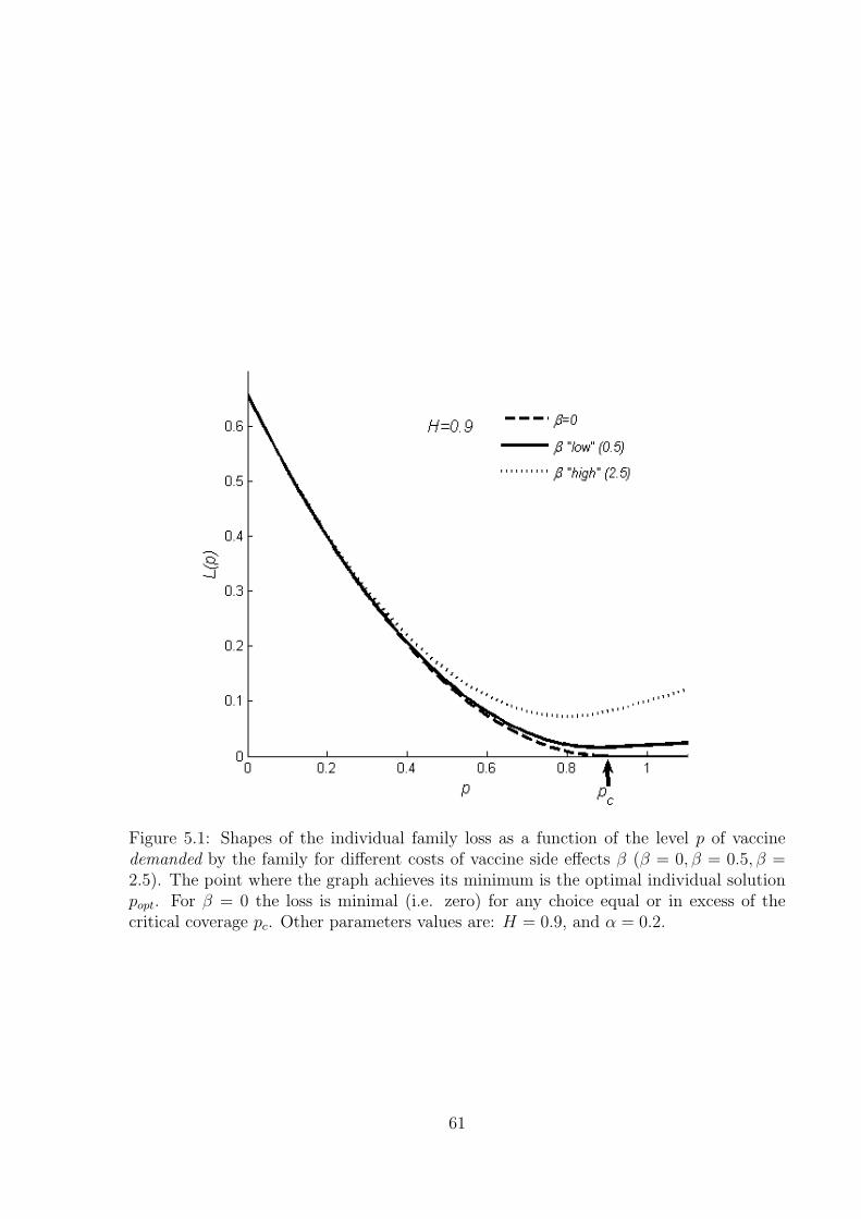
Figure 5.1: Shapes of the individual family loss as a function of the level p of vaccinedemanded by the family for different costs of vaccine side effects β (β = 0, β = 0.5, β =2.5). The point where the graph achieves its minimum is the optimal individual solutionpopt. For β = 0 the loss is minimal (i.e. zero) for any choice equal or in excess of thecritical coverage pc. Other parameters values are: H = 0.9, and α = 0.2.

61

to the case of informed families, and in particular close to 100% if the cost of VSE isnegligible. Under the same parameters assignments of the example above we find thatfor β = 0.5, the optimal coverage is near 98%, and even for β = 2.5 it is about 89%, i.e.still quite close to pc. It follows that lack of information on the existence of the infectionthreshold seems therefore to provide a simple explanation of how patterns of universalvaccination might emerge in actual circumstances.

5.2.3 Only a fraction of the population is eligible

An interesting case is when only a fraction f1 of the population is eligible for vaccination,for example because of the presence of a group practicing conscientious exemption. Inthis case the overall vaccination coverage is defined as p1 = pf1, and the critical coveragethat needs to be achieved in the eligible population is p?c = pc/f1 > pc, which might begreater than one if the eligible fraction is small. In the case of informed families we get

popt

H2f2

1

βα2 +H2f 21

pcf1

= ε1p?c if ε1p

?c < 1

1 elsewhere

(5.9)

This result will be useful in the next section.

5.3 Implications of strategic behavior: the game-

theoretic approach

5.3.1 A preliminary: the critical elimination line for multigrouppopulations

Let us now consider a SIR-type disease in a population subdivided into two groups withfrequencies f1, f2, and heterogeneous coverages p1, p2. If the population is homogeneouslymixing the collective coverage is p = p1f1 + p2f2 and the elimination rule (p ≥ pc) forvaccination at birth becomes:

(5.10) p1f1 + p2f2 ≥ pc

showing that the possibility of elimination depends not only on groups’ actual coveragesbut also on their frequencies. Taking the frequencies as given, (5.10) states that elimina-tion requires coverages p1, p2 in the two groups lying above a critical line (CL). The CL isthe portion lying in the unit vaccination square [0, 1]× [0, 1] (i.e. the space of admissiblevaccination policies), of the straight line p1f1 + p2f2 = pc, which can be written as:

(5.11) p1 = p?1,c −f2f1p2

62

where p?1,c = pc/f1. Any pair (p1, p2) lying above the CL would eliminate the infection.The CL has negative slope (an increase in critical coverage in group 2 allows a reductionin group 1 without compromising elimination) m = −f2/f1, reflecting the relative size ofthe two groups. The intercept p?1,c and the foot p?2,c = pc/f2 represent the vaccinationeffort that would be required to either group to eliminate infection when the other groupdoes not vaccinate. If either p?1,c, p

?2,c exceeds 1 elimination is unfeasible without some

cooperation.

By means of the CL we may answer useful questions related to the containment of theimpact of anti-vaccinators on control programs, e.g. if group 2 vaccinates above threshold,to what extent can group 1 vaccinate below threshold without compromising elimination?Let us consider (Fig.5.2a) a disease with R0 = 5 (sometimes adequate for rubella) implyingpc = 0.8, in a community where group 2 represents 90% of the population (f2 = 0.9).The foot p?2,c ' 0.89 indicates that group 2 can achieve elimination alone. However thesteepness of the CL (m = −9) indicates that small departures from this level make itnecessary to vaccinate also in group 1. If coverage in group 2 is 85%, then eliminationrequires at least 35% coverage in group 1.

To sum up, the shape of the CL reflects both the difficulty to eliminate the disease,summarized by pc (which in turns reflects transmissibility through the increasing relationpc = 1 − 1/R0), shifting upward when, other things being equal, pc increases, and therelative size of the two groups. Fig.5.2b illustrates the possible forms of the CL. Theseforms correspond to distinct socio-epidemiological types: (a) the CL entirely lies withinthe vaccination square: this is characterized by the condition pc < min{f1, f2} and impliesthe case of a moderately transmissible infection, i.e. such that pc < 1/2 ⇔ R0 < 2, withgroups of not too dissimilar size (pc < f1 < 1 − pc); (b) both the intercept and the footof the CL lie outside the vaccination square: this corresponds to a highly transmissibleinfection (pc > 1/2 ⇔ R0 > 2) and groups of not too dissimilar size; (c) the intercept liesoutside and the foot inside: this is expressed by the condition f1 < pc < f2. This case iscompatible with very large differences in size between the two groups when R0 approaches1 or when it is very large (R0 >> 2); (d) the intercept lies inside the and the foot outside;this is just the symmetric of (c) when the roles of the two groups are interchanged (notreported in the figure).

Given our focus on the possibility to eliminate a highly transmissible disease in pres-ence of a small group with low vaccine uptake, the type of major interest for our discussionis (c). It is important to remind that in this case group 2 is large enough to eliminatewithout cooperation from group 1, i.e. p?2,c < 1. This means that if for instance R0 = 15,so that pc = 0.93, the maximal affordable size of the anti-vaccine group is less than 7%.

5.3.2 The vaccination game

In a game-theoretic framework, unlike the individual optimization of section 2, families(players) make their choices by taking into considerations other families’ decisions. Weassume that families are subdivided into two groups of fixed (no migration between thegroups is allowed) sizes f1 and f2. Families are characterized by homogeneous preferences

63

Figure 5.2: (a) Vaccination square, critical line, and elimination zone for a disease withR0 = 5 (pc = 0.8) in a community where group 2 is majority (f2 = 0.9); (b) Differentshapes of the CL corresponding to the three different socio-epidemiological types: type a:R0 = 1.4, f1 = 0.35; type b: R0 = 3, f1 = 0.4; type c: R0 = 3, f1 = 0.3

within the group they belong to, but heterogeneous preferences between groups. Thisallows to refer to a representative agent for each group. Group 1 (anti-vaccinators)3

has a higher relative cost of VSE (β1 > β2 ≥ 0) as in [36], and it is smaller (f1 <1/2). We focus on the case of informed families, but the extension to non fully informedfamilies is straightforward. The informed representative family of each group determinesits vaccination propensity pj (j = 1, 2) by solving the problem:

(5.12) MinpjLj = (ρI(p))2 + βjα

2p2j j = 1, 2; 0 ≤ p1, p2 ≤ 1

where the perceived risk of infection is, as before, given by:

ρI(p) =

H(pc − p) if p < pc

0 elsewhere(5.13)

In particular p = p1f1 + p2f2 (the constraint 0 ≤ p1f1 + p2f2 ≤ 1 is always fulfilledas 0 ≤ p1, p2 ≤ 1, 0 ≤ f1, f2 ≤ 1) represents the overall coverage that would follow from

3We have made the distinction between pro and anti-vaccinators just for labeling the two groups. Theonly difference between the two types of agents lies in the different perceived costs following from theirdecisions (as a consequence perhaps of using distinct information sources), and neither imply distinctapriori propensities to vaccinate nor a larger apriori cooperative attitude. However we will see that thesedifferent costs imply that a posteriori one group will be more inclined to vaccinate than the other. Thisresults from the competition within groups as a Nash strategy within group.

64

choices (p1, p2) of families of the two groups. In other words families know that the overallcoverage depends on their choices (i.e. from people of their group) but also on the othergroup choices. Given that choices made by either group produces some effects also onthe other group, solving (5.12) and (5.13) requires to make assumptions as to the typeof strategic game families play. We will consider simultaneous games, non simultaneousgames (also termed Stackelberg games), and social planner games [110].

5.3.3 The basic strategic competition

In this case the two groups decide their action simultaneously by taking as given theaction of the other group. The Nash solution to (5.12) and (5.13) uses the concept ofvaccination reaction function. The reaction function M1(p2) (M2(p1)) of players of group1 (2) defines the optimal vaccination choice of player 1 (2) corresponding to any feasiblevaccination choice 0 ≤ p2 ≤ 1 of players from group 2 (1). The points where the tworeaction functions intersect are Nash Equilibria [110]. The algebraic determination of thereaction functions, though elementary, requires a tedious computation to consider all thepossible cases, depending on the type of the Critical Line, and on the values of the costsβi. For sake of simplicity we just summarize the main graphic features of M1(p2) (whichhold mutatis mutandis for M2(p1)):

1 since the risk of infection is positive only in the region below the CL (see (5.13)), itis intuitive that the reaction functions will be positive only in such a region;

2 if group 2 is able to eliminate without cooperation from group 1 (f2 large enoughthat p?2,c), then every p2 choice in excess of p?2,c is a feasible elimination choice. Inthis case M1(p2) is identically zero for p?2,c ≤ p2 ≤ 1;

3 if group 2 is not large enough to eliminate alone (p?2,c > 1), then M1(p2) is positivefor all 0 ≤ p2 ≤ 1;

4 if the value popt1 determined in section 2.3, which represents the intercept M1(0),exceeds 1 (this can happen if p?1,c > 1), a portion of M1(p2) will lie flat on the upperboundary of the vaccination square;

5 the positive portion of M1(p2), will be decreasing in p2 to mirror that as group 2increases its demand for vaccines, group 1 will find it convenient to vaccinate less(and symmetrically for M2(p1)). This is found by optimizing L1 in the region belowthe CL, yielding:

(5.14) popt1 (p2) =f 21H

2

β1α2 + f 21H

2(p?1,c +

f2f1p2) = ε1(p

?1,c +

f2f1p2)

with 0 < ε1 < 1. The line (5.14) is always flatter than the Critical Line, and it hasthe same foot. By finally relating the possible shapes of M1(p2) to the underlyingtypes of the CL (Fig.5.2b) we obtain the forms represented in Fig.5.3.

65

Figure 5.3: Possible shapes of the reaction function M1(p2) of group 1 in relation to theunderlying types of the Critical Line.

66

A special but important case occurs when families of group 2 assign a zero cost tovaccine side effects (β2 = 0). In this case the internal portion of the reaction functionM2(p1) will always coincide with the Critical Line.

Finally, as for the case of not-fully informed families, it seems natural to assume thatat least families of group 2 are not aware of herd immunity, and therefore obey (5.5)-(5.6).This will imply, other things being equal, a reaction function M2 having a higher interceptand the same slope.

We can now collect our results. They are summarized in Fig.5.4 for a variety ofdifferent circumstances. For brevity we only discuss the case of type (c), that is the mostimportant for our purposes. For generality we consider two distinct possibilities as for therelative cost of VSE in group 1: β1,low = 1, β1,high = 2.5 and take β2 < β1,low. The caseβ1,high corresponds to a very low reaction function of group 1, which vaccinates little evenif group 2 does not vaccinate, whereas in the case β1,low group 1 vaccinates 100% at verylow vaccination choices of group 2. In particular Fig.5.4a, 5.4b, 5.4c deal with the case ofinformed families, while Fig.5.4d with the case of non-fully informed agents. If the relativecost of VSE in group 2 is positive, however small (Fig.5.4a), then the Nash equilibrium,i.e. the intersection between the reaction functions, will lie strictly below the Critical Line,indicating that the families’ behavior is not compatible with elimination. When group2 does not suffer costs from VSE (β2 = 0) then (Fig.5.4b) the internal portion of thereaction function of group 2 coincides with the CL, and the Nash equilibrium is locatedat the foot p?2,c of the CL. In this case elimination is feasible because group 2 is largeenough to support the whole elimination effort without any cooperation from group 1.Note however that if group 2 is not sufficiently large, then elimination becomes impossibleeven in the favorable case β2 = 0 (Fig.5.4c). Indeed a larger anti-vaccine group make theCL (and M2) flatter, so that the Nash equilibrium is pushed out of the vaccination square.If families of group 2 do not know herd immunity then, other things being equal, M2

moves upward (Fig.5.4d) and can therefore always lie above the CL. In this case the Nashequilibrium locates above the elimination threshold. Therefore lack of knowledge of theelimination threshold make elimination possible even when this was not the case underfully informed agents. The previous results therefore prove the following:

Result 1 (Elimination is impossible under informed families). As long as both groupsassign a positive value to the cost of VSE (β1, β2 > 0) elimination is never possible.Elimination is possible if pro-vaccinators do not suffer costs from VSE (i.e. β2 = 0) andtheir group size is large enough to sustain elimination without the cooperation of theother group.

Summarizing, in presence of informed families, the forces operating in the Nash caseare never able to promote a coverage above the critical one. This provides the mainrationale for compulsory vaccination as the rule to avoid non-cooperative Nash behavior.

When families are not aware of herd immunity, then, as noted in section 2, circum-stances are more favorable to elimination (as in Fig.5.4d). Nonetheless high costs of VSEand increases in the size of the anti-vaccine group can obviously lead to a communitycoverage below the critical threshold in this case as well.

67

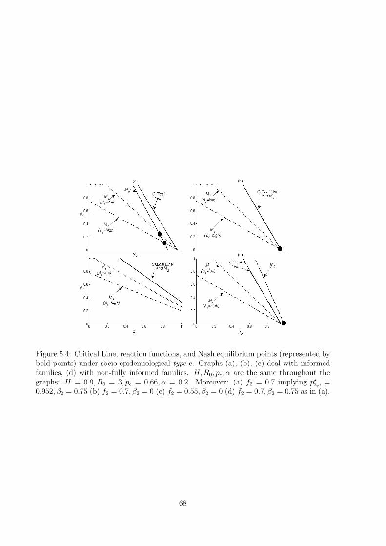
Figure 5.4: Critical Line, reaction functions, and Nash equilibrium points (represented bybold points) under socio-epidemiological type c. Graphs (a), (b), (c) deal with informedfamilies, (d) with non-fully informed families. H,R0, pc, α are the same throughout thegraphs: H = 0.9, R0 = 3, pc = 0.66, α = 0.2. Moreover: (a) f2 = 0.7 implying p?2,c =0.952, β2 = 0.75 (b) f2 = 0.7, β2 = 0 (c) f2 = 0.55, β2 = 0 (d) f2 = 0.7, β2 = 0.75 as in (a).

68

We finally note that the coordinates of the Nash equilibrium can be computed explic-itly:

pNash1 =

H2f1β2

H2(f 21β2 + f2

2β1) + α2β1β2

pc

pNash1 =

H2f2β1

H2(f 21β2 + f2

2β1) + α2β1β2

pc

(5.15)

so that the corresponding overall coverage is:

(5.16) pNash = pNash1 f1 + pNash

2 f2 =H2(f 2

1β2 + f 22β1)

H2(f 21β2 + f 2

2β1) + α2β1β2

pc

which immediately shows our main result: pNash ≤ pc.

5.3.4 The Stackelberg case with anti-vaccinators leadership

In Stackelberg games4 there is a leader who minimizes its loss function by taking intoaccount the reaction function of the follower, rather than by taking it as given, as inthe previous section. This implies therefore a behavioral asymmetry, that might be con-sistent with the vaccination game in developed countries where anti-vaccinator groupstend to be very active in the information acquisition and decision processes. To modelthis anti-vaccinators leadership in our framework we assume that anti-vaccinators havean information advantage, i.e. they know pro-vaccinators behavior (i.e. their reactionfunction) and incorporate it into their loss function.

We therefore assume that families from group 2 play as before, thereby computing theirreaction function M2(p1), whereas families from group 1 know M2(p1), and incorporate itinto their own loss function. Thus group 1 determines its optimal vaccination choice pStack1 ,and group 2 will as a consequence follow by just recomputing its choice as M2(p

Stack1 ). In

the case of informed families it holds:

(5.17) pStack1 =f 21H

2(1− ε2)2

f21H

2(1− ε2)2 + α2β1

pc

where

ε2 =f22H

2

α2β2 + f 22H

2

It is thus easy to see that when both groups have positive costs of VSE, the elim-ination impossible result continues to hold. In addition it is possible to prove that inthe Stackelberg equilibrium (pStack1 ,M2(p

Stack1 )) the demand for vaccines by group 1 will

4Stackelberg games are usually compared with Cournot games when distinguishing sequential andsimultaneous play. Both types of games can have strategies satisfying Nash’s criteria [140].

69

be lower compared to the basic simultaneous game of section 3.2, while that of group 2will be consequently higher. The intuition for such a result is that when group 1 acts asStackelberg leader it has the advantage to decide its optimal policy by considering theentire reaction of group 2 to its own behavior. For instance group 1 knows that if itdecides not to vaccinate, group 2 will entirely bear the burden of the (whole) commu-nity immunization (included the cost of VSE). No surprise, then, that in such a case thevaccination effort of group 1 will be lower than in the case in which the two groups playsimultaneously.

5.3.5 The social planner case

The elimination impossible trap under Nash or Stackelberg rules suggests to look at thepossibility that a social planner may attempt to find an agreed solution. To this end,we consider a social loss function L = L(p1, p2) of a utilitarian type [110], defined as aweighted average of the loss functions of the two groups. The social planner will finda socially optimal solution by minimizing the social loss function and then will seekappropriate policy tools to actually implement the optimal solution among the two groups.He will solve:

(5.18) Minp1,p2 xL1 + (1− x)L2 0 ≤ x ≤ 1

where x is the weight that he assigns to the loss of group 1. This case requires someelaboration (see appendix in [109]), but its results are easy to understand. We onlyconsider the case of fully informed families. In this case no solution can lie above the CL(p ≥ pc): in fact the partial derivatives of the social loss function L are always non negativeand do not vanish simultaneously. Looking for solutions lying below the CL, standardcomputations yield the following optimum point, i.e. the so called Nash equilibrium inthe social planner case:

pSoc1 =

{p2 if p1 < 11 elsewhere

(5.19)

pSoc2 =

p2 if p1 < 1

H2f22 (p

?2,c − f1/f2)

H2f 22 + (1− x)β2α2

elsewhere

where

p1 =(1− x)f1H

2β2

H2((1− x)f 21β2 + xβ1f 2

2 ) + x(1− x)α2β1β2

pc

p2 =(1− x)f2H

2β1

H2((1− x)f 21β2 + xβ1f 2

2 ) + x(1− x)α2β1β2

pc

(5.20)

70

One thus immediately notes that for values of the weight x belonging to (0, 1) it holds:pSoc = pSoc1 f1 + pSoc2 f2 < pc. This means that when both groups concur to form thesocial loss function, and in presence of informed families with positive costs from VSE,elimination is impossible even under social planning.5 Nonetheless, the present case yields,in most situations, a higher coverage compared to both Stackelberg and Nash cases. Thiscan be better understood from the limit cases where the social planner assigns a unitweight to either groups. These cases are discussed easily. Note instead that if x = 1 then:

(5.21) pSoc1 = p1 = 0; pSoc2 = p2 = p?2,c

Therefore under type c, there exists an optimal social planning solution which allowselimination. On the other hand, if x = 0 then: p1 = p?1,c > 1 and p2 = 0. Therefore

(5.22) pSoc1 = 1; pSoc2 =f 22H

2

f 22H

2 + β2α2

(p?2,c −

f1f2

)It is easy to see that this solution does not allow elimination since it yields an overall

coverage lower than pc:

pSoc = pSoc1 f1 + pSoc2 f2

= f1

(1− f2H

2

f2H2 + β2α2

)+ pc

f2H2

f2H2 + β2α2< pc

(5.23)

To sum up, for x = 1 social planning yields a feasible elimination policy if group 2 is largeenough to eliminate alone.

The overall implications of different weights given by the social planner to the twogroups in the social loss functions are illustrated (Fig.5.5) for a highly transmissible diseasewith R0 = 10 (pc = 0.9) and f2 = 0.9. This means p?c2 = 1.0, i.e. that a vaccine demandof 100% in group 2 would be required to achieve elimination when group 1 does notvaccinate. In addition we assume that group 2 has a cost of VSE smaller than the costof infection (β2 = 0.75) whereas for group 1 this cost is much higher (β2 = 2.5). Ithappens (Fig.5.5a) that the vaccine demand in group 1 is constant at 100% (pSoc1 = 1)for very small x values, but as x exceeds a threshold value it starts to fast decline up tozero. Similarly, the vaccine demand in group 2 is initially constant at a level around 76%,but when the vaccine demand of group 1 starts declining it starts increasing and reachesuniversal coverage for x = 1. As regards the overall coverage (Fig.5.5b) this is initiallyconstant around the level of 78%, but when coverage in group 2 starts increasing it startsincreasing as well, achieving the elimination threshold pc = 0.9 for x = 1. All this isconsistent with our theoretical findings. It is interesting to note that social planning doesnot necessarily yields an improvement of the Nash solution (the flat line in Fig.5.5b): thishappens only when the vaccine demand in group 2 becomes sufficiently high, which does

5It is possible to envisage other social planner functions, based on very different perspectives, thatmight lead to elimination.

71

Figure 5.5: The social planner case. (a) the optimal vaccine demand in groups 1,2(pSoc1 , pSoc2 ) as functions of the weight x attributed to group 1 in the social loss func-tion; (b) Overall vaccine demand (pSoc) versus the corresponding quantity in the Nashcase. Parameter values: R0 = 10, β1 = 2.5, β2 = 0.5, α = 0.2, f1 = 0.1.

not occur if x is close to zero.6 Note also that if the social planner assigns to group 1 aweight proportional to its demographic frequency (x = 0.1), which a priori could appeara reasonable choice, an overall coverage of 87.7% follows, which is better than the Nashcoverage.

The results for x = 1 and x = 0 lead to interesting remarks. Note that for x = 1elimination does not require that β2 = 0, as in the Nash and Stackelberg cases. Theexplanation is that for x = 1 the preferences (i.e. the costs) of group 2 are not taken intoconsideration by the social planner (whereas those of group 1 fully are), so that group 1achieves its optimum (not vaccinating at all), and then group 2 needs to supply residuallythe amount of vaccination needed to minimize the social loss function. It happens thatthis amount is, consistently with the frequencies of the two groups, the one requiredto eliminate the disease. In more concrete terms, for x = 1 the social planner giveswhole weight to the preferences of anti-vaccinators, and no weight to the preferences ofvaccinators, on the assumption that this is a good way to achieve the social optimumi.e. disease elimination. This means that vaccinators contribute fully altruistically to the

6We note that the Nash solution results slightly better than the Stackelberg one (not reported in thefigure). Moreover under not-fully informed families an increase in the overall coverage will follow, in linewith our previous findings.

72

social optimum, since they entirely supply the elimination effort. It is also interesting tonote that the opposite case (x = 0), i.e. full weight to the pro-vaccinators preferences, isthe one yielding the worse result in terms of coverage, even worse of the non-cooperativeNash outcome.

5.4 Discussion: can we get off the no-elimination

trap?

A variety of models of vaccination choice, both without and with strategic behavior, havebeen investigated, under both informed, and not-fully informed agents.

The analysis of the non-strategic choice indicates that informed families knowing theherd immunity principle will always vaccinate below the critical threshold as soon as theysuffer any, however small, cost of VSE, while a high collective coverage is much morelikely to be achieved if families are not aware of herd immunity. The analysis of thestrategic case, carried out on the assumption of the existence of a vast (fixed) majority ofagents having a small perceived cost of VSE (labeled as pro-vaccinators) versus a minorityhaving a high perceived cost of VSE (anti-vaccinators), confirms that in presence of fullyinformed families disease elimination continues to be impossible unless pro-vaccinators donot associate any cost to vaccine side effects, and moreover their frequency is in excess ofthe critical elimination coverage. If anti-vaccinators lead the game, i.e. in the Stackelbergcase, the outcome in terms of coverage will be worse compared to the Nash case. Evenif the State aims at favoring cooperative behavior through social planning, elimination ispossible only when the State takes into account in the social loss functions the prefer-ences of anti-vaccinators only7. This scenario seems to be representative of the currentItalian situation, where the possibility to switch from a compulsory to a voluntary vac-cination system is actively debated, and one region, Veneto, has recently made the step[60]. In this context, under the pressure of anti-vaccinators, the Italian government hasgradually accepted an increasing number of right claims by anti-vaccinators, for exampleit has removed the parents’ duty to vaccinate their children in order to enroll them tocompulsory school grades. This can be interpreted as a massive increase of the weight ofanti-vaccinators in the social loss function. Our results indicate that a social planning pol-icy of this sort, i.e. paying more weight to anti-vaccinators, seems to be technically correct(in fact in the opposite case, where the State takes into account the preferences of pro-vaccinators only, dramatically low coverage would follow, even worse than the Stackelbergoutcome.). However such static results figure out the possible dynamic unsustainabilityof such a policy. Indeed, how to prevent migrations towards the anti-vaccine choice, ifthis starts to be more generally perceived as more protective of children’s health? Thoughthe consideration of migration between groups would require a dynamic model (as [15]),

7Clearly this result relies upon the adopted form of the social loss function. This does not excludethat other social planner functions, based on different perspectives, for example including the Governmentloss, could allow to achieve elimination under weaker conditions. We thank an anonymous referee for thisremark.

73

we note that global socio-economic trends are not favorable in this sense: empirical stud-ies indicate that often those vaccinating less are the more educated, or the richer, ones[18, 142]. One can certainly invoke the economic argument that no free-rider groups canexpand above a certain threshold. In epidemiological terms this means that any furtherexpansion in the anti-vaccinator group will decrease the degree of herd immunity andwill therefore be stopped by the necessary re-emergence of the disease. The public healthdangerousness of such a situation, think for instance to slow declines in herd immunitydue to slow migrations toward the anti-vaccinator group, call for a careful monitoring ofsuch processes.

The case of not fully informed families produces, as a rule, better outcomes. However italso raises substantive questions. Which information mechanisms cause real communitiesto polarize into a majority who usually vaccinates universally, and a very active minoritywho is strongly reluctant to vaccinate? Our model static is not capable of explainingpolarization (it just postulates it) it strongly suggests that universal vaccination in themajority follows from: a) a very small cost associated to VSE, b) the lack of knowledgeof the critical threshold, i.e. parents believing that a propensity to vaccinate of 100% isnecessary to fully protect children against disease. This wrong perception (mathematicstells indeed that the critical threshold for disease elimination is always less, sometimessubstantially less, than 100%) is the likely cause of the asymmetry of the real worldvaccination game. Asymmetry stems from the fact that certain group of agents mightinstead have a correct knowledge of herd immunity. But this asymmetry is dangerousfor the public health system since it implies the uneven situation where someone takesthe risks of vaccine side effects to protect all, as a consequence of limited information.This further enhances the danger that people improve their information set, and as aconsequence rationally migrate towards the anti-vaccinator group.

In conclusion, do we need to fear RE? Mathematics shows that RE can be devastat-ing for immunization programs [16, 15, 36, 48, 49], [131]. This is especially true whenrumors, e.g. the MMR scare [135], contribute to disproportionately increase perceivedrisks of vaccine associated side effects compared to the perceived risk of infection [142].As regards remedies against RE, first economic papers on the subject [23, 72] suggestedthat the free-rider problem might partly be overcome through e.g. taxes and subsidies. Arecent modeling effort [124] has shown that the free-rider effect may be amplified by theassumption of homogeneous mixing, and that the problem can be largely reduced whenmore realistic contact networks are considered. Be things as they may, the actual impactof vaccination free-riding is hard to predict: RE is human behavior, which, as recentlypointed out, is a missing factor of our epidemiological explanation [56].

However, better mathematical models could help to improve our understanding ofsuch phenomena, and to design more informative studies of vaccination behavior, possi-bly aimed to also capture strategic parameters. On the other hand we believe that forthose public health systems that have already initiated a roadmap towards voluntary vac-cination, as in Italy is the case of Veneto region [60], investment in education to the socialrole of vaccination will be an unavoidable task in the future.

74

Chapter 6

The impact of vaccine side effects onthe natural history of immunizationprograms: an imitation-gameapproach

6.1 Introduction

Although forms of exemption to vaccination have always existed [139], the ”natural his-tory” of vaccination programmes, as part of the historical pathway through which hu-mankind progressive rids itself of infectious diseases, has always been pervaded by a highdegree of optimism [30]. However, recently this optimistic view has increasingly been chal-lenged: for example, opposition to the whole-cell pertussis vaccine [70], the thimerosalcase [106], and the MMR scare [135] can be considered evidence that in industrializedcountries, the success story of vaccination is feeding back on itself. This is the conse-quence of two different processes. On the one hand, the high degree of herd immunityachieved by decades of successful immunization programmes has reduced the incidence ofmany infections to negligible levels. On the other hand the large, and increasing, numberof vaccines routinely administered every year yields steady flows of vaccine-associated sideeffects [160], [159]. In the US approximately 30,000 reports of Vaccine Adverse Eventsare notified annually, with 10–15% classified as serious [62]. In such circumstances theperception of the public will likely rank the perceived risk of suffering a vaccine side effect(VSE) as much higher than the corresponding risk of infection [16, 15, 48, 49]. A commonexample is poliomyelitis in industrialized countries. For example in Italy during 1980-2000 the number of vaccine-induced polio cases was three times higher than wild poliocases [43]. Under voluntary vaccination high degrees of herd immunity might thereforeincentivise vaccination free riding [23],[131], i.e. the parents’ decision not to vaccinatechildren after comparing the perceived risk of disease and the perceived risk of vaccineside effects [16, 15, 48]. Vaccination free riding [23, 61, 72, 16, 15, 48, 49, 46, 131, 129, 69]makes eradication impossible (unless special contact structures are considered [124]) and

75

triggers stable oscillations in the infection prevalence.Previous studies on the impact of vaccination free riding on endemic infections havefocused on scenarios where the vaccine demand is driven by the time changes in the per-ceived risk of disease, measured through the current (or past) infection prevalence. Basedon the above-cited literature on VSEs we instead suggest that in industrialized countries,where the incidence of common vaccine preventable infections is very low, the availableinformation on vaccine side effects might become the main driving force of vaccine de-mand. The only paper devoted to this issue is [46], where, however, vaccine demand wasphenomenologically modelled as a decreasing function of the perceived risk of suffering avaccine-associated side effect. The perceived risk of VSEs was in its turn evaluated by thepublic from available information on current and past trends of side effects attributed tothe vaccine. In this paper we shift the focus onto the impact of VSEs on the dynamics ofimmunization programmes for endemic infections, using an SIR transmission model withvoluntary vaccination choice. Vaccination choices are described by an evolutionary gameas in [15], where the vaccine uptake p(t) is determined by an imitation process betweenagents (the parents of the children to be vaccinated) who are divided into ”vaccinators”and ”non-vaccinators”. However, in [15] the perceived payoff of the ”non-vaccinators”is proportional to the prevalence of the disease, whereas the payoff of ”vaccinators” isconstant, i.e. independent of VSEs).The novelty of the present work is that the payoff of ”vaccinators” is proportional tothe incidence of vaccine-associated side effects. In turn, this incidence is proportionalto the actual vaccine uptake. We believe that this model represents a more appropriatedescription of the future evolution of immunization programmes in voluntary vaccinationregimes. Indeed, the fact that available information on vaccine side effects might becomethe main driving force of vaccine demand is strongly supported by the empirical evidence,e.g. the case of England and Wales, where due to the MMR scare[135], first dose measlesuptake fell for several years from 94% to about 75%. Compared to [15] we also expand ourbasic model to include (a) nonlinear perceived costs of infection; (b) the possibility thatthe perceived costs of infection and vaccination are evaluated by the public using pastvalues of state variables, for example due to information delay [49] or of the perceptionof long-term vaccine side effects [46].

6.2 Materials and Methods

6.2.1 Dynamic vaccine demand and vaccine side effects

We consider a family of models of the spread of a non-fatal SIR infection controlled byvoluntary vaccination with a ”perfect” vaccine administered in a single dose at birth and

76

giving life-long immunity:

S ′ = µ(1− p)− µS − βSI(6.1)

I ′ = βSI − (µ+ ν)I(6.2)

p′ = k1∆Ep(1− p)(6.3)

where: S, I are the susceptible and infective fractions, and p the vaccinated proportionamong newborn children; β > 0, µ > 0, ν > 0 denote the transmission, the mortality andthe recovery rates. We assume that, in absence of vaccination, the disease is endemic, i.e.R0 = β/(µ+ ν) > 1.The dynamics of p obeys a learning by imitation [81] process where k1 is the ”imitation”coefficient and switching between the decisions to vaccinate or not to vaccinate, is de-termined by the payoff gain ∆E(t). The latter is given by the difference between theperceived payoff of vaccinators −ρV (t), where ρV (t) is the perceived risk of suffering aVSE, and the perceived payoff of non-vaccinators: −ρI(t), where ρI(t) is the perceivedrisk of suffering serious illness due to infection.We note that, irrespective of the specific forms of ∆E(t), the family of models (6.1-6.2-6.3) has the following three equilibria: (i) an unstable disease-free equilibrium with novaccinators A = (1, 0, 0); (ii) a pure-vaccinator disease-free equilibrium B = (0, 0, 1); (iii)the pre-vaccination equilibrium C =

(SSIR = R−1

0 , ISIR = µ(1−R−10 )/(µ+ ν), 0

).

The stability of B and C and the existence of further equilibria depend on the specifictypes of the payoff gain.Modelling of the dynamics of p by an imitation game was introduced in the seminalpaper [15], where a specific model of the family (6.1-6.2-6.3) was proposed, where: i)the perceived payoff of vaccinators is constant:−ρV = −rV ; and ii) the perceived payoffof non-vaccinators is proportional to the infective prevalence I(t): −ρI(t) = −rImI(t),where mI(t) is an estimate of the current risk of infection, and rI is the risk of seriousdisease as a consequence of infection. Hence:

∆E(t) = rImI(t)− rV = rV (ϑI(t)− 1) ,

where ϑ = mrI/rV is proportional to the relative cost of the non-vaccinator strategy.In Bauch’s model the B equilibrium is unstable and there is a fourth equilibrium: thepost-vaccination equilibrium D =

(R−1

0 , ϑ−1, p)where: p = (1 + ν/µ) (ISIR − ϑ−1) . At

ϑ = ϑ0 = I−1SIR there is a transcritical bifurcation between C and D. In turn, the stabil-

ity/instability of D depends on the product k1(ϑ− ϑ0).The assumption in [15] that the perceived risk of vaccination ρV (t) is constant can bejustified if the public correctly evaluates this risk as the ratio between total VSEs perunit time, given by α (µN) p(t) (α ∈ (0, 1)) where N is the total population size (so thatµN is the yearly number of births), and α the per-capita probability of incurring a VSEduring a single vaccine administration, and the total number of vaccinations administeredfor that specific disease µNp(t). We instead suppose that the public evaluates the risk ofVSEs by using the available information on the total number of vaccine-associated side

77

effects, or, which is equivalent, on the ratio between the total number of vaccine associatedside effects and the total number of newborn children per unit of time. We therefore set:

(6.4) ρV (t) = αp(t)

The implication of (6.4) is that periods of large vaccine uptake negatively feed back,through an increase in the incidence of VSEs, into the proportion of parents favourableto vaccination.We model the perceived risk of infection as an increasing function h1(·) ≥ 0 of the informa-tion index M , introduced in [48, 49], that summarizes the publicly available informationon the infection:

(6.5) ρI(t) = h1(M(t)).

The indexM , used by agents to evaluate the risk of infection, may model not only current,but also past information. The case h1(0) > 0 accounts for the scenario where the diseaseis locally eliminated but disease re-emergence by external reintroduction is feared. In thesimplest case, the information index M(t) is related to the current I(t) as follows:

(6.6) M(t) = h2 (I(t)) ,

where h2(·) > 0 and h′2 (·) > 0. Using (6.4)-(6.5)-(6.6) the dynamics of p can be written

as follows:

(6.7) p′ = k (h(I)− p) p (1− p)

where h(I) = α−1h1(h2(I)), k = αk1.First, note that from: p′ ≥ k (h(0)− p) p (1− p) it follows that h(0) ≥ 1 ⇒ p(t) → 1, sothat we shall not consider this trivial case. On the contrary, if h(0) < 1 then p(t) ≥ h(0)holds asymptotically, i.e. the collective coverage will at least reach the minimal level h(0).Symmetrically, inequality p′ ≤ khMaxp (1− p) means that p(t) is bounded by a logisticdynamics with kinetics constant khMax. Finally, if imitation dynamics is faster than theinfection time scale: k >> (µ+ ν)−1, then p(t) is at quasi-equilibrium:

(6.8) p(t) ≈ min (h (M(t)) , 1) ,

which is the phenomenological relationship first proposed in [48].

6.2.2 The importance of time delays

The assumption that ∆E depends only on current values of I and p is an approximation.For example agents might perceive that vaccines are responsible for VSEs arising with longtime delays [46], as might be the case with auto-immune diseases [116]. Moreover, delaysof different nature, concerning the information on the spread of the disease, may involve

78

both p(t) and M(t) [48]. Thus in the case in which the perceived risk of vaccination isevaluated on past VSEs:

(6.9) ρV (t) =

∫ t

−∞QH(Tv)αp(t− Tv)dTv

where QH is a delay kernel. An important kernel is the exponentially fading memory :QH(x) = bExp (−bx) , b > 0, which allows reduction to ODE since it holds that:

(6.10) ρ′V = b (αp(t)− ρV ) .

Scenarios such as long-term VSEs may require different kernels, more concentrated onpast periods, such as the Erlang functions: Anx

n−1Exp(−bx), also allowing reduction toODEs.

6.3 Results

6.3.1 Endemic equilibria and their stability

In this section we shall investigate the model (6.1)-(6.2)-(6.7) where no delays are present.Considering a generic h(I), the system (6.1)-(6.2)-(6.7) has three equilibrium points A(unstable), B (unstable) and C, which, unlike [15], is always unstable since the linearizedequation for p reads η′ = kh (ISIR) η. Moreover, two further equilibria are induced by thespecific ∆E we introduced:

• A disease-free equilibrium with positive vaccine uptake Edfe = (1− h(0), 0, h(0)).

• A new behaviour-related endemic equilibrium:

Ebeh =(R−1

0 , Ie, h (Ie)),

where Ie is the unique solution of the equation:

(6.11) h(I) = 1−R−10 − µ+ ν

µI.

Remark 6.3.1. The equilibrium Ebeh is equal to the endemic equilibrium of the modelstudied in [46], where, however, p is not a state variable.

Since all equilibria are independent of k, this makes it natural to choose k as a bifurcationparameter. Our main results (demonstrated in the Appendix 8.3) are as follows:

A) If

(6.12) βIeµh′ (Ie) < (µ+ βIe)

((µ+ βIe) + 2

√βIe(µ+ ν)

)then Ebeh is locally asymptotically stable (LAS) irrespective of the imitation speedk;

79

B) On the contrary, if

(6.13) βIeµh′ (Ie) > (µ+ βIe)

((µ+ βIe) + 2

√βIe(µ+ ν)

)holds then there are two positive values k1 and k2 > k1 such that:

1. If 0 < k < k1 or k > k2 then Ebeh is LAS;

2. At k = k1 and at k = k2 there are Hopf bifurcations;

3. If k ∈ (k1, k2) then Ebeh is unstable.

C) In the case k ∈ (k1, k2) the orbits x(t) = (S(t), I(t), p(t)) are oscillatory in the senseof Yabucovich. This intuitively means that for sufficiently large t all state variablesare permanently oscillating, with regular or irregular oscillations. Formally, forj = 1, 2, 3 it holds that:

minlimt→+∞xj(t) < maxlimt→+∞xj(t).

D) If h0 > pc then Edfe is globally asymptotically stable (GAS); if h0 < pc then Edfe isunstable.

Remark 6.3.2. Note that the r.h.s. of (6.13) is O(µ3/2), whereas µβIe is O(µ2), implyingthat to have Hopf bifurcation at Ebeh the derivative of h there has to be at least of orderO(µ−1/2)

Remark 6.3.3. Property D shows that, unlike [15], elimination is possible in our model,although only if in absence of the disease the vaccinator payoff is so large as to yield avaccine uptake greater than the elimination threshold.

To better understand the phenomenon of epidemic oscillations driven by vaccinationchoice we compare the above results with the recent literature on this subject. Unlike [15]where large values of k (ϑ− ϑ0) induce sustained oscillations around the endemic state, inour model oscillations are possible in an intermediate window of values of the imitationcoefficient k. This means that both slow and fast imitation are stabilizing forces. More-over, we note that the stability condition (6.12) has the same formal structure as that ofthe delayed model in [48], where dependence of the current vaccine uptake on past inci-dence was required to obtain oscillations. Indeed, imitation is a (nonlinear) adjustmentprocess introducing a delay, whose characteristic time scales are determined by the speedwith which the vaccine uptake reacts to changes in the payoff gain. Heuristically, close tothe equilibrium eq. (6.7) becomes:

(6.14) p′ ≈ kh (Ie) (1− h (Ie)) (h (I)− p) = Ψ (h (I)− p)

which may be read as an exponentially fading memory mechanism with average delay1/Ψ. This suggests a route to estimate the elusive imitation coefficient k, by preliminar-ily estimating the average delay 1/Ψ.

80

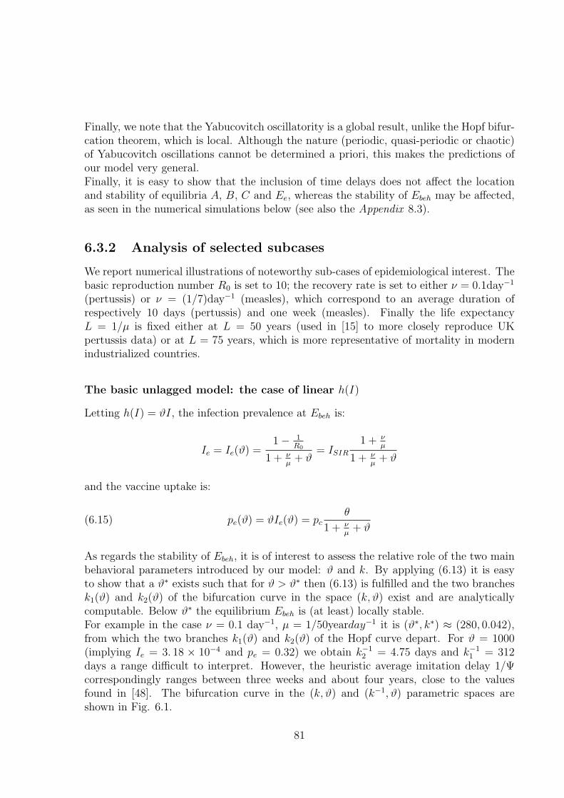
Finally, we note that the Yabucovitch oscillatority is a global result, unlike the Hopf bifur-cation theorem, which is local. Although the nature (periodic, quasi-periodic or chaotic)of Yabucovitch oscillations cannot be determined a priori, this makes the predictions ofour model very general.Finally, it is easy to show that the inclusion of time delays does not affect the locationand stability of equilibria A, B, C and Ee, whereas the stability of Ebeh may be affected,as seen in the numerical simulations below (see also the Appendix 8.3).

6.3.2 Analysis of selected subcases

We report numerical illustrations of noteworthy sub-cases of epidemiological interest. Thebasic reproduction number R0 is set to 10; the recovery rate is set to either ν = 0.1day−1

(pertussis) or ν = (1/7)day−1 (measles), which correspond to an average duration ofrespectively 10 days (pertussis) and one week (measles). Finally the life expectancyL = 1/µ is fixed either at L = 50 years (used in [15] to more closely reproduce UKpertussis data) or at L = 75 years, which is more representative of mortality in modernindustrialized countries.

The basic unlagged model: the case of linear h(I)

Letting h(I) = ϑI, the infection prevalence at Ebeh is:

Ie = Ie(ϑ) =1− 1

R0

1 + νµ+ ϑ

= ISIR1 + ν

µ

1 + νµ+ ϑ

and the vaccine uptake is:

(6.15) pe(ϑ) = ϑIe(ϑ) = pcθ

1 + νµ+ ϑ

As regards the stability of Ebeh, it is of interest to assess the relative role of the two mainbehavioral parameters introduced by our model: ϑ and k. By applying (6.13) it is easyto show that a ϑ∗ exists such that for ϑ > ϑ∗ then (6.13) is fulfilled and the two branchesk1(ϑ) and k2(ϑ) of the bifurcation curve in the space (k, ϑ) exist and are analyticallycomputable. Below ϑ∗ the equilibrium Ebeh is (at least) locally stable.For example in the case ν = 0.1 day−1, µ = 1/50yearday−1 it is (ϑ∗, k∗) ≈ (280, 0.042),from which the two branches k1(ϑ) and k2(ϑ) of the Hopf curve depart. For ϑ = 1000(implying Ie = 3. 18 × 10−4 and pe = 0.32) we obtain k−1

2 = 4.75 days and k−11 = 312

days a range difficult to interpret. However, the heuristic average imitation delay 1/Ψcorrespondingly ranges between three weeks and about four years, close to the valuesfound in [48]. The bifurcation curve in the (k, ϑ) and (k−1, ϑ) parametric spaces areshown in Fig. 6.1.

81

0 0.1 0.2 0.3 0.4 0.5 0.6 0.7 0.8 0.90

500

1000

1500

2000

2500

3000

3500

4000

4500

5000

k

thet

a

0 10 20 30 40 50 60 70 80 90250

300

350

400

450

500

550

T=(1/K) days

The

ta

0 0.1 0.2 0.3 0.4 0.5 0.6 0.7 0.8150

200

250

300

350

400

450

500

K

The

ta

0.5

0.75

0.85

Figure 6.1: Bifurcation curve for linear and linear affine h(I), in the case R0 = 10, ν =1/10 day−1, , µ = 1/50 year−1. (left-hand panel) Bifurcation curve for linear h(I) = ϑIin the parameter space (k, ϑ). (Central panel) Bifurcation curve for linear h(I) = ϑIin the parameter space (k−1, ϑ) emphasizing patterns for small imitation-related delays.(Right-hand panel) Bifurcation curve for linear affine h(I) = p0 + ϑI plotted for threevalues of p0. As p0 increases the minimal threshold of ϑ is non-monotone.

The basic unlagged model: the case of linear-affine h (I)

The case h(I) = ϑ0 + ϑI is of interest since it assumes that even in scenarios of zeroprevalence agents perceive a positive risk ϑ0 of infection re-emergence. We get:

Ie(ϑ) =1−R−1

0 − ϑ0

1 + νµ+ ϑ

, pe(ϑ) = ϑ0 + ϑ1−R−1

0 − ϑ0

1 + νµ+ ϑ

Thus the perception of such a risk has a positive effect on equilibrium uptake. Thedependence of the bifurcation curve on ϑ0 may be non-monotone, as in the right-handpanel of Fig. 6.1.

6.4 Substantive implications of vaccine side effects

for vaccination programmes

6.4.1 The epidemiological transition and vaccination payoff

We use equilibrium results from the simple case of linear h(I) to explore the impactof human progress on the natural history of vaccination programmes. Note that in theparametric set we are considering the quantity ν/µ ranges from about 1826 (pertussis in apopulation with low life-expectancy) up to about 3913 (measles in a population with highlife-expectancy). Thus, achieving a large equilibrium uptake requires very large ϑ, i.e. ofthe order of ν/µ. Since ϑ = rIm/α, it follows that to achieve large equilibrium uptakesfor measles or pertussis, the perceived cost of serious disease has to be at least three orderof magnitude higher than the perceived cost of VSE. Though this seems surprising, wefeel it is consistent with what was still observed at the beginning of the 20th century,when the risk of serious sequelae following measles or scarlet fever was extremely large(100-250 deaths per 100000 cases of disease), and the absence of vaccines was keeping therisk of infection very high. In such circumstances even a large probability of suffering a

82

VSE from a vaccine could have been tolerated by the community. This also suggests thatin industrialized countries the recent (say after 1970-1980) ’big vaccination age’ is comingto an end due to the completion of the epidemiological transition [143], i.e. the historicalchange in the cause composition of mortality from infectious and nutritional diseases tochronic degenerative ones. Indeed, an outcome of the transition has been the dramaticfall in the levels of serious morbidity and mortality from all infectious diseases. Finally,as regards the role played by life expectancy on the steady state Ebeh, our results suggestthat the achievement of a given equilibrium uptake in industrialized countries (i.e. witha very high life expectancy) requires a much larger value of ϑ compared to developingcountries. This is consistent with the fact that in regimes with low mortality (also as aconsequence of vaccinations), agents demand a vaccine only if the relative risks of sufferinga VSE are very low. We stress that our predictions are equilibrium ones based on a simpledeterministic model with homogeneous mixing. Nonetheless more realistic models wouldnot substantially affect them.

6.4.2 Simulations

In our simulations we set h(I) = ϑI and, to better emphasize our main messages, we allowimmigration of infectives, according to two different hypotheses: a) a small constanttransfer Imm from the susceptible to the infective state, representing a steady flow ofinfections as a consequence of international travelling; b) a few new infections appearat some stage once and for all, in order to mimic the possibility of infection resurgence.Indeed, in the oscillatory regime the infection prevalence I(t) may reach extremely lowvalues, which calls into question the appropriateness of a deterministic model. Thisdrawback is avoided by assumption a, also used in [15]. Imm is set to one infectiveindividual per week in a population of 5× 106 individuals.

The basic unlagged model

We first assess the impact of VSEs on the transient infection dynamics triggered by anew vaccination introduced at the pre-vaccination endemic state, and under assumptiona. The vaccine is introduced at time t = 0, with initial vaccine uptake set to 0.95 > pc.Vaccine side effects occur from the beginning of the programme. We set ϑ = 15000(implying pe ≈ 0.71, k = 0.002 day−1 and 1/Ψ ≈ 7 years). Note that k is small since it isthe product between the natural imitation rate and the low probability α of suffering aVSE. As predicted by (6.13), the system converges, in epidemiologically reasonable timescales, to a stable limit cycle. With reference to Fig. 6.2, the vaccine uptake (right-handpanel) starts declining soon after the programme starts, due to the onset of VSEs, and fallsbelow the critical threshold pc in less than four years. Thus the effective reproductionnumber RE(t) = R0 ∗ S(t) (left-hand panel) initially declines but then increases andexceed the unit threshold at t ≈ 8 years, yielding a new epidemic outbreak at t ≈ 10years. During this rather long ’honey-moon’ period the circulation of the infection isessentially sustained by immigration. Note that p(t) > pc for a rather long period of

83

0 20 400.85

0.9

0.95

1

1.05

1.1

time (years)

RE(t)

0 20 400

1

2

3

4

5

6

7

8x 10

−4

time (years)

I(t)

0 20 40

0.4

0.5

0.6

0.7

0.8

0.9

1

time (years)

p=pc

p(t)

Figure 6.2: The unlagged model with linear h(I): dynamics of RE(t) (left-hand panel),I(t) (centre), p(t) (right-hand panel), following the initiation of an immunization pro-gramme with p(0) = 0.95; S0, I0 fixed at their pre-vaccination endemic state. Parameters:R0 = 10, ν = 1/7 day−1, , µ = 1/75 year−1, θ = 15000,k = 0.002 day−1.

time (about 36 per cent of total time). During such periods routine vaccination surveyswould reveal a satisfactorily high coverage. Therefore they could not explain the endemicpersistence of infection.The role played by k is illustrated in Fig. 6.3, which considers the values: k = 0.0005,k = 0.002 (as before), k = 0.0035, and which shows that: i) the average uptake is notsignificantly affected by k and remains close to pe; ii) both the amplitude of oscillationsof p(t) and the fraction of total time where p(t) > pc increase in k; iii) the duration of theperiod between the start of the programme and a new epidemic outbreak is decreasingin k. For example, the ’low’ k value (k = 0.0005) yields oscillations that are of smallamplitude and that for a small portion of their period are such that p(t) > pc. Moreover,there is an interval of about 17 years about before a new epidemics, which is only a fewyears long for k = 0.0035. This is the consequence of the slow spread of informationoccurring for low k, which slows down the reactivity of the vaccine uptake to changesin the payoff gain. Note that if no external infections are introduced, then for small kthe infection prevalence is close to zero. This suggests that oscillations might producestochastic elimination of infection.We now study the introduction of a new vaccine for which no vaccine side effects areinitially known. In this case it seems reasonable to assume that an intermediate periodmight exist during which no perception of VSEs arises. We consider α = 0 for t < t1where t1 = 10 years, and that the starting point is the pre-vaccination steady state. Ofcourse, the vaccine uptake start increasing since the payoff vaccination is initially positive(α = 0). If VSEs raise after a very long time, or no VSEs are reported, then stochasticelimination is possible. By contrast, if evidence of VSEs emerges, the scenario reducesstraightaway to the cases treated above. If the imitation process is very slow, VSEs appearbefore reaching a sufficient coverage and a sub-optimal vaccination coverage is achieved

84

0 20 40

0.4

0.6

0.8

1

p(t)

0 20 400

2

4

6

8x 10

−4

time (years)

I(t)

0 20 40

0.4

0.6

0.8

1

0 20 400

2

4

6

8x 10

−4

time (years)

0 20 40

0.4

0.6

0.8

1

0 20 400

2

4

6

8x 10

−4

time (years)

p=pc

Figure 6.3: The unlagged model with linear h(I): dynamics of p(t) (top) and I(t) (bot-tom), for k = 0.0005 (left), k = 0.002 (centre), k = 0.0035 (right) following the initiationof an immunization programme with p(0) = 0.95; S0, I0 fixed at their pre-vaccinationendemic state. Other parameters: R0 = 10, ν = 1/7 day−1, , µ = 1/75 year−1, θ = 15000.

(left-hand panel of Fig. 6.4). Instead for a larger value of k, the infective fraction isvery close to 0 such that stochastic elimination may occur (central panel of Fig. 6.4).Finally, for an intermediate range of k there is onset of oscillations, but at the end of theirtransitory the minimum I(t) is very close to 0 and elimination can again occur (right-handpanel of Fig. 6.4).Finally, we simulated the case where eradication was achieved thanks to a period ofcompulsory vaccination, after which vaccination becomes voluntary. In this case VSEsinduce individuals to switch to the ’non-vaccinator’ strategy, thereby producing a decreasein vaccination coverage. This in turn increases the probability of infection re-emergencefrom imported cases. If a few new external infections are introduced (assumption b) beforeRE(t) = 1, then the occurrence or not of stochastic transient elimination depends againon k, with patterns similar to the previous case (see Fig. 6.5.a,6.5.b,6.5.c). Moreover, ifindividuals take into account a non zero risk of infection re-emergence from importation(the linear affine case h(I) = ϑ0 +ϑI), the population is more ’protected’ and the impactof the external infections can be reduced also for large values of k (see Fig. 6.5.d).

85

years

Infe

ctio

ns

0 100 200 300 400

00.

0001

250.

0002

50.

0003

755e

−04

0R

e=1

0.25

0.5

0.75

1

years

Infe

ctio

ns

0 12.5 25 37.5 50

00.

0001

250.

0002

50.

0003

755e

−04

0R

e=1

0.25

0.5

0.75

1

years

Infe

ctio

ns

0 50 100 150 200

00.

0007

50.

0015

0.00

225

0.00

3

0R

e=1

0.25

0.5

0.75

1

Figure 6.4: Dynamics of I(t) (black line), R0S(t) (dotted black line), p(t) (dashed blackline) with (a), k = 0.0001 (b) and k = 0.001 (c). The vertical grey dashed line describethe time in which elimination occur. The vertical grey line describe the time in which VSEappears. Initial conditions: S(0), I(0) fixed at pre-vaccination endemic state, p(0) ' 0.Other parameters: R0 = 10, ν = 1/10 day−1, , µ = 1/50 year−1, θ = 5000.

years

Infe

ctio

ns

0 3 6 9 12

02.

5e−

065e

−06

7.5e

−06

1e−

05

00.

250.

50.

751

1.25

years

Infe

ctio

ns

0 3 6 9 12

00.

0012

50.

0025

0.00

375

0.00

5

00.

250.

50.

751

1.25

years

Infe

ctio

ns

0 3 6 9 12

02.

5e−

065e

−06

7.5e

−06

1e−

05

00.

250.

50.

751

1.25

Figure 6.5: Left and central panels: dynamics of I(t) (black line), R0S(t) (dotted blackline), p(t) (dashed black line) for θ = 5000,h0 = 0. and p(0) = 0.95, S(0) = 1 − p(0),I(0) = 10−5. Left-hand panel k = 0.001. Central panel: k = 0.01. The black line is thethreshold pc. Right-hand panel: as the central panel but for h0 = 0.7,p(0) = 0.80 andS(0) = 0.07. Other parameters: R0 = 10, ν = 1/10 day−1, , µ = 1/50 year−1, θ = 5000.

Impact of information-related delays

An exponentially distributed lag in the p term yields a model given by (6.1)-(6.2) com-plemented by:

(6.16) p′ = k (h(I)−H)) p (1− p)

and by (6.10). Fig. 6.6 reports the stability regions in the (k, b) plane for ϑ = 260,ϑ ≈ 279.5 (which is close to the critical value ϑ∗ in absence of delays) and ϑ = 500. Notethat for ϑ = 500 > ϑ∗ for all b there are two values kl(b;ϑ) and kr(b;ϑ) such that forkl(b;ϑ) < k < kr(b;ϑ) the endemic state Ee is unstable and it is also an easy matter toshow that Yabucovitch oscillations can arise. Similar plots are obtained in all cases whereϑ > ϑ∗. This can be easily explained since for very large b the lagged model reduces tothe unlagged one that, for ϑ > ϑ∗, has an instability interval.Interestingly, the right panel of 6.6 for ϑ = 260 < ϑ∗ shows instability regions that are

86

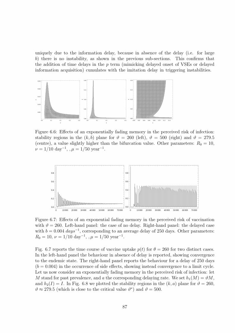
uniquely due to the information delay, because in absence of the delay (i.e. for largeb) there is no instability, as shown in the previous sub-sections. This confirms thatthe addition of time delays in the p term (mimicking delayed onset of VSEs or delayedinformation acquisition) cumulates with the imitation delay in triggering instabilities.

0.0 0.1 0.2 0.3 0.4

0.005

0.010

0.015

0.020

0.025

k

b

0.0 0.1 0.2 0.3 0.40.00

0.05

0.10

0.15

0.20

k

b

0.00 0.02 0.04 0.06 0.08 0.10 0.12 0.14

0.00

0.05

0.10

0.15

0.20

k

b

Figure 6.6: Effects of an exponentially fading memory in the perceived risk of infection:stability regions in the (k, b) plane for ϑ = 260 (left), ϑ = 500 (right) and ϑ = 279.5(centre), a value slightly higher than the bifurcation value. Other parameters: R0 = 10,ν = 1/10 day−1, , µ = 1/50 year−1.

0 10 000 20 000 30 000 40 000 50 000 60 000 70 000

0.0

0.2

0.4

0.6

0.8

0 10 000 20 000 30 000 40 000 50 000 60 000 70 000

0.0

0.2

0.4

0.6

0.8

Figure 6.7: Effects of an exponential fading memory in the perceived risk of vaccinationwith ϑ = 260. Left-hand panel: the case of no delay. Right-hand panel: the delayed casewith b = 0.004 days−1, corresponding to an average delay of 250 days. Other parameters:R0 = 10, ν = 1/10 day−1, , µ = 1/50 year−1.

Fig. 6.7 reports the time course of vaccine uptake p(t) for θ = 260 for two distinct cases.In the left-hand panel the behaviour in absence of delay is reported, showing convergenceto the endemic state. The right-hand panel reports the behaviour for a delay of 250 days(b = 0.004) in the occurrence of side effects, showing instead convergence to a limit cycle.Let us now consider an exponentially fading memory in the perceived risk of infection: letM stand for past prevalence, and a the corresponding delaying rate. We set h1(M) = ϑM ,and h2(I) = I. In Fig. 6.8 we plotted the stability regions in the (k, a) plane for ϑ = 260,ϑ ≈ 279.5 (which is close to the critical value ϑ∗) and ϑ = 500.

87

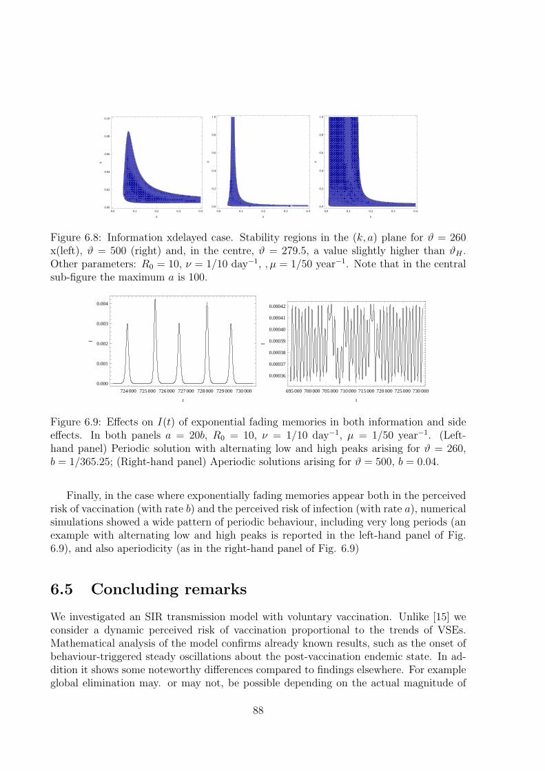
0.0 0.1 0.2 0.3 0.40.00

0.02

0.04

0.06

0.08

0.10

k

b

0.0 0.1 0.2 0.3 0.4

0.0

0.2

0.4

0.6

0.8

1.0

k

b0.0 0.1 0.2 0.3 0.4

0.0

0.2

0.4

0.6

0.8

1.0

k

b

Figure 6.8: Information xdelayed case. Stability regions in the (k, a) plane for ϑ = 260x(left), ϑ = 500 (right) and, in the centre, ϑ = 279.5, a value slightly higher than ϑH .Other parameters: R0 = 10, ν = 1/10 day−1, , µ = 1/50 year−1. Note that in the centralsub-figure the maximum a is 100.

724 000 725 000 726 000 727 000 728 000 729 000 730 000

0.000

0.001

0.002

0.003

0.004

t

I

695 000 700 000 705 000 710 000 715 000 720 000 725 000 730 000

0.00036

0.00037

0.00038

0.00039

0.00040

0.00041

0.00042

t

I

Figure 6.9: Effects on I(t) of exponential fading memories in both information and sideeffects. In both panels a = 20b, R0 = 10, ν = 1/10 day−1, µ = 1/50 year−1. (Left-hand panel) Periodic solution with alternating low and high peaks arising for ϑ = 260,b = 1/365.25; (Right-hand panel) Aperiodic solutions arising for ϑ = 500, b = 0.04.

Finally, in the case where exponentially fading memories appear both in the perceivedrisk of vaccination (with rate b) and the perceived risk of infection (with rate a), numericalsimulations showed a wide pattern of periodic behaviour, including very long periods (anexample with alternating low and high peaks is reported in the left-hand panel of Fig.6.9), and also aperiodicity (as in the right-hand panel of Fig. 6.9)

6.5 Concluding remarks

We investigated an SIR transmission model with voluntary vaccination. Unlike [15] weconsider a dynamic perceived risk of vaccination proportional to the trends of VSEs.Mathematical analysis of the model confirms already known results, such as the onset ofbehaviour-triggered steady oscillations about the post-vaccination endemic state. In ad-dition it shows some noteworthy differences compared to findings elsewhere. For exampleglobal elimination may. or may not, be possible depending on the actual magnitude of

88

the baseline perceived risk of disease relative to the risk of vaccine side effects. As regardsthe pre-vaccination equilibrium, differently from [15], it is always unstable, so that anyvaccination programme will initially be successful, at least partially. Moreover oscillationsoccur, provided the relative risk of disease is large enough, in a bounded window of theimitation parameter. In addition, we also considered the impact of time delays on thevaccination payoff gain, which is a realistic feature. Finally, the model allows notewor-thy inferences on the future lifetime of vaccination voluntary programmes. It suggeststhat in order to achieve high equilibrium uptakes for e.g. measles, the perceived cost ofthe disease must be at least three orders of magnitude higher than the perceived cost ofvaccine-associated side effects, and moreover that this requirement is further increasedunder situations with large life expectancies. Both these facts seem to be consistent withreal world observations, and suggest that maximal vaccination effort by international in-stitutions should target increasing vaccine uptake in less developed countries where therisk of serious sequelae is still high, and life expectancy is still low. Simulations finallyprovide further interesting insights on the effect of behavioural parameters on vaccineuptake.

89

90

Chapter 7

Conclusion

As recently pointed out, human behavior is a relevant missing factor of epidemiologicalmodeling [56, 52].

In fact, organized measures such as quarantine or closure of public places are one waythat behavior can change, but people may also spontaneously modify their behavior toreduce perceived risk.

Results presented in my thesis show that spontaneous behavioral response to epi-demics, coming either from the concern about the infection or from possible vaccine sideeffects, can remarkably affect the epidemic spread both qualitatively and quantitativelyand may also compromise the expected outcome of voluntary vaccination programs andother control measures. Indeed, human behavioral changes may alter timing, dynamicsand overall number of cases during a (severe) epidemic outbreak while the problem ofrational exception may be responsible of drops in vaccine uptake and suboptimal vaccinecoverage and may trigger the resurgence of diseases for which the current prevalence isvery low.

Evidences about spontaneous social distancing and other self-imposed prophylacticmeasures in response to emerging outbreaks, have been reported for past epidemics [98,59, 90, 136, 144]. On the other hand, a large number of countries, whose vaccinationpolicies are based on voluntary compliance, are increasingly facing the challenge of refusalof vaccines caused by high concerns about proclaimed risks from vaccine side effects[70, 106, 89, 135, 64, 142, 163]. Thus, spontaneous behavioral responses, not accountedby large majority of transmission models, can not be neglected to correctly inform publichealth decision makers.

The class of models developed in this thesis project provides a promising approach,based on evolutionary game theory, to investigate the complex interaction between humanbehavior and diseases transmission process, contributing to assess possible effects derivingby risk perception and individual choices.

When studying the spread of epidemics, behavior and contact patterns are typicallyconsidered as a “background” for the infection process– i.e., they are not variables of thedynamics. For mild infections such approximation is justified, as individuals rarely funda-

91

mentally change their behavior because of symptoms associated to diseases auch as cold.On the other hand, the evidence shows that faced with lethal or novel pathogens, peoplewill change their behavior to try to reduce their risk [56]. In these cases, population be-havior cannot be merely considered as an independent (though time-varying) parameter,but it is better modeled as a variable whose evolution influences, and is influenced by, thedynamics of the infection.

Actually, the diffusion of human beliefs can be driven by mechanism similar to thosedriving an epidemic; different source of information can be considered for the spreadof information in a population (e.g., rumors, media, ... ). Recently, models have beenproposed for investigating spontaneous social distancing describing human behavioralresponses as driven by the diffusion of fear, which is modeled as a parallel infection[147, 42, 53, 93, 67, 66]. However, evolutionary game theory – that is a natural frameworkfor studying human behavior – provides an alternative way for modeling the diffusion ofresponsiveness in the population.

Models introduced in chapters 2, 3, 4, 6 couple the transmission dynamics with animitation process, i.e. a learning process, in which the convenience of self-protection (e.g.,the reduction of the number of potentially infectious contacts or the choice to vaccinate)is assessed trough personal encounters. Human behavior is assumed to be driven by theevaluation of prospective outcomes deriving from alternative decisions and cost-benefitconsiderations that depend on the perceived prevalence of infection and, in the case ofvoluntary vaccination choices, the incidence of vaccine side effects (possibly consideringtime delays and memory mechanisms).

With the introduction of explicit models for behavioral changes based on evolutionarygame theory, infection and behavior both contribute to define the context for the other.Symmetry between these two key-factors is therefore restored, and no by-principle preva-lence is given (even formally) to one over the other. Not only the infection dynamicsdepends on both the transmission and behavior, but also the behavior dynamics dependson behavior (and infection as well). This is what makes evolutionary game theory espe-cially suited to this situation as compared to classical game theory. In fact, applicationof the latter would result in (rational) instantaneous best responses to the infection dy-namics, regardless of the current distribution of behavioral strategies. On the other hand,at first sight, introduction of irrational behavior may appear unnecessary, and contrast-ing with models simplicity. Yet, by avoiding extinction of allowed behaviors, irrationalbehavior overtakes an unrealistic (and undesirable) effect of strict imitation: the pool ofstrategies from which an individual can choose is limited to those effectively representedin the population. On the other hand, by allowing exploration of all possible behaviors,irrational behaviors may account for erroneous decisions or idiosyncratic attitudes alwayspresent in human societies.

Independently of how the risk is specifically reckoned, the access to information per-taining the relative efficacy of behaviors may also be collected across more structurednetworks (e.g., the media). In this respect, considering different time units adds someflexibility to models developed, in that it allows for different speeds in the diffusion ofinfection and behavior. For example, tuning of key parameter driving the speed of behav-

92

ioral changes (e.g., ε in chapter 2, ρ in chapters 3,4 and k in chapter 6) may be obtainedon the basis of empirical evidence.

More structured models, as for instance individual based models and network models,may be more appropriate for investigating actual situations and empirical data. How-ever, it is worth of noticing that the approach proposed is fairy general to be appliedfor describing any kind of disease (e.g. influenza, smallpox, SARS, measles, varicella,pertussis) and, it can be easily included into more structured models in order to accountfor spontaneous human behavior.

The simple model introduced in chapter 2 allows the investigation of the dynamics ofspontaneous reduction in the number of contacts, performed as a protective response tothe state of the epidemic and the spread of a (severe) disease. That is why the behav-ioral change modeled here affects only susceptible individuals (infected individuals mayof course change behavior as an effect of their status, regardless of the state of epidemic).The proposed model couples an SIR model with selection of behaviors driven by imitationdynamics. Therefore, infection transmission and population behavior become dynamicalvariables that influence each other. In particular, time scales of behavioral changes andof epidemic transmission can be different. The performed analysis provide a full qualita-tive characterization of the solutions when the dynamics of behavioral changes is eithermuch faster or much slower than that of epidemic transmission. For suitable parameterconfigurations, the model accounts for multiple outbreaks occurring within the same epi-demic episode. Moreover, the model can explain “asymmetric waves”, i.e. infection waveswhose rising and decaying phases differ in slope. Finally, it is proved that introduction ofbehavioral dynamics can lead to a reduction of the final attack rate.

In chapter 3, an extension of the model introduced in chapter 2, including a widerclass of scenarios, is presented. The model of behavioral changes is extended to infectedindividuals subgrouped in symptomatic and asymptomatic, treating the infected asymp-tomatic as susceptibles for anything concerning the behavioral dynamics. The impact ofkey features of a human self-protection on the effectiveness of behavioral responses arediscussed. The analysis of the proposed model highlights that, if the perceived risk asso-ciated to an epidemic is sufficiently large, even small behavioral changes can remarkablyreduce the final epidemic size and the daily peak prevalence. Moreover, if the delay inthe behavior diffusion – embedded in the imitation process – is not too large, the re-sponse of the population is always effective. The population responsiveness increases asthe symptomaticity increases, while memory of past cases and initial overestimation ofthe risk of infection essentially delay the epidemic spread. Results of this study are con-sistent to those obtained by previous works through different assumptions. Specifically,as shown in [42], the disease spread results highly sensitive to how rapidly people adopta self-reduction in their contact activity rates. Moreover, if behavioral changes are fastenough, they can have a remarkable effect in reducing the daily infection prevalence [93]and the final epidemic size [67]. Finally, as in [53], for suitable parameter configurations,

93

the epidemic dynamics can account for multiple epidemic waves.

In chapter 4 the approach introduced in chapter 3 is used for investigating the 2009H1N1 pandemic influenza dynamics in Italy. As it emerges from the analysis of influenza-like illness incidence data, after an initial period characterized by a slow exponentialincrease in the weekly incidence, a sudden and sharp increase of the growth rate is ob-served. The performed investigation, based on model fit to epidemiological data and onthe analysis of antiviral drugs purchase, reveals that an initial overestimation of the riskin the general population, possibly induced by the high concern for the emergence of anew influenza pandemic, can result in a pattern of spread compliant with the observedincidence. Moreover, the analysis of influenza-like illness incidence data highlights thatthe estimation of fundamental epidemiological parameters (and in particular of the repro-ductive number) may be reconsidered as well, as it could be largely affected by humanbehaviors.

Static models for vaccination choice introduced in chapter 5 allow getting some mean-ingful insights on disease elimination feasibility under voluntary vaccination policy. First,the elimination impossible result is proved by a simple model of individual choice in pres-ence of informed families, i.e. families aware of herd immunity, and it is suggested thatlimited information might explain patterns of universal vaccination. Next, vaccinationchoices are investigated in a game-theoretic framework for communities stratified intotwo groups, pro and anti vaccinators, having widely different perceived costs of infectionand of vaccine side effects. Under the assumption of informed families neither a Nashnor a Stackelberg behavior (characterized respectively by players acting simultaneouslyand by an asymmetric situation with a leader and a follower) allow disease elimination,unless pro-vaccinators assign no costs to vaccine side effects. Elimination turns out tobe possible when “cooperation” is encouraged by a social planner, provided however heincorporates in the social loss function the preferences of anti-vaccinators only.

Finally, the model with dynamic vaccine demand, based on imitation and describedin chapter 6, may represent a significant contribution for the investigation of the problemof rational exception. Here the perceived risk of vaccination is modeled as a function ofthe incidence of vaccine side effects, instead of using a constant. This represents the maininnovative aspect of the model. The impact of time delays on the vaccination payoffs isconsidered as well. Mathematical analysis of the model confirms already known results,such as the onset of behavior-triggered steady oscillations about the post-vaccination en-demic state. The model shows important differences compared to previous game dynamicmodels of vaccination. For example, global elimination may, or may not, be possible de-pending on the actual magnitude of the baseline perceived risk of disease relative to therisk of vaccine side effects. Differently from [15], the pre-vaccination equilibrium is alwaysunstable, so that any vaccination program will initially be successful, at least partially.Moreover, provided the relative risk of disease is large enough, oscillations occur in abounded window of the imitation parameter. The performed analysis suggests that, in

94

order to achieve high coverages, a huge disproportion between the perceived risk of diseaseand vaccination is necessary. This disproportion is further increased in highly industri-alized countries. Both these facts seem to be consistent with “real world” observations,and suggest that maximal vaccination effort by international institutions should targetincreasing vaccine uptake in less developed countries where the risk of serious sequelae isstill high, and life expectancy is still low.

As regards the problem of rational exception in vaccination choices, noteworthy in-ferences emerged in the analysis of proposed models need to be properly discussed. Thepossibility to switch from a compulsory to a voluntary vaccination system is actively de-bated, and one Italian region, Veneto, has recently made the step [60]. In epidemiologicalterms, any further expansion in the anti-vaccinator group will decrease the degree of herdimmunity and will therefore be stopped by the necessary re-emergence of the disease.Though the consideration of migration between groups would require a specific dynamicmodel, global socio-economic trends are not favorable in this sense: empirical studies in-dicate that often those individuals vaccinating less are the more educated, or the richer,ones [18, 142]. The public health dangerousness of such a situation, think for instance toslow declines in herd immunity due to slow migrations toward the anti-vaccinator group,call for a careful monitoring of such processes.

Moreover, the investigation performed in chapters 5 and 6 strongly suggest that uni-versal vaccination in the majority of the population follows from: a) a very small costassociated to vaccine side effects, b) the lack of knowledge of the critical threshold, i.e.parents believing that a propensity to vaccinate of 100% is necessary to fully protect chil-dren against disease. This wrong perception (mathematical models show that the criticalthreshold for disease elimination is always less, sometimes substantially less, than 100%)is dangerous for the public health system since it implies the uneven situation wheresomeone takes the risks of vaccine side effects to protect all, as a consequence of limitedinformation. This further enhances the danger that people improve their information set,and as a consequence, rationally migrate towards the anti-vaccinator group. Thus, forthose public health systems that have already initiated a road map towards voluntaryvaccination, as in Italy is the case of Veneto region [60], investment in education to thesocial role of vaccination will be an unavoidable task in the future.

After all, considering models accounting for spontaneous behavioral changes would behelpful for giving insight to public health policy makers for planning public health controlstrategies during an emerging epidemic (also providing better estimates about the burdenfor health care centers over time) and for evaluating the effectiveness of control measuresbased on voluntary compliance.

However, as regards spontaneous behavioral changes occurring during an epidemicoutbreak, “the challenge for mathematical modelers is that data are scarce, and oftenqualitative when they do emerge”, as pointed out in [56]. Actually, few efforts have been

95

made to validate models dealing with spontaneous behavioral changes from empiricalobservations.

The study performed in chapter 4 may represent a further step in this direction, as thequantitative and qualitative effects of spontaneous behavioral changes in the populationon the spread of an epidemic have been validated against empirical data. However, atthe current stage, the proposed models could hardly be used for real time predictionssince our knowledge on plausible values of model parameters related to human behavioris only preliminary. Further investigations have to be performed in order to gain a majorconsciousness on how such mechanisms work.

Undeniably, a lot of empirical data would be needed for models validation and parametriza-tion. However, recent surveys on human behavioral response have started to answer ques-tions as: where people obtain their information from, which of information available tothem they trust, if and how they act upon the information [90, 82, 39, 98, 144].

On the other hand, the chance of considering reliable data on human behavior increasesin the context of vaccination. Indeed, data on vaccine uptake may represent also humanbehavior and would allow quantitative estimation, model validation and, in turn, a betterunderstanding of mechanisms that drive information and beliefs diffusion and the interplaybetween risk perception and the spreading responsiveness during epidemics.

96

Chapter 8

Appendix

8.1 Appendix A

8.1.1 Proofs

Proof of Proposition 2.3.2

S1 Let us consider the set T1 = {0}∪{t > 0 | I(t) < 1/m ∀ t ∈ (0, t)}. T1 6= ∅ and let usdefine t1 = supT1. I(0) := I0 < 1/m implies that t1 > 0. Let us consider any finitetime t < t1. For any t ∈ [0, t], the boundary–layer system (2.9) with I = I(t) admitsthe asymptotically stable equilibrium x?(I), as defined in Eq. (2.10) and x?(I) → 1when µ → 0 (see Prop. 2.3.1). In fact, I(t) < 1/m for each t ∈ [0, t]. Therefore, thesolution of the degenerate system (2.8) is equivalent to that of a classical SIR modelwith R0 = Rn

0 on the whole interval [0, t]. By Tikhonov theorem [148], this is alsothe approximation of the solution of system (2.5). Condition 1/m < Ip guaranteesthat t1 < +∞. In fact, if t1 = +∞, system (2.5) is equivalent to an SIR modelwith R0 = Rn

0 and thus I(t) = Ip > 1/m for some finite time t > 0, which impliest1 6= supT1. Moreover, I(t1) = 1/m.

S2.1 Let us now assume that Ra0S(t1) ≤ 1. As observed in the main text, the only

admissible value for the fraction of infected individuals is I(t) = 1/m+O(ε) as longas Rn

0S(t) > 1. Formally, if I(t) > 1/m in some interval then x(t) would be veryclose to 0 in almost the whole interval. Thus, I(t) would be negative and I(t) woulddecrease below 1/m. On the other hand, if I(t) < 1/m in some interval then x(t)would be very close to 1. Thus, I(t) would be positive and I(t) would increase over1/m.

This has two relevant consequences, namely

• in the slower time scale system we havedI

dt(t) = 0;

• in the faster time scale system we havedx

ds(s) = 0 since µ = o(εk) with k ≥ 1

(see Eq. 2.9). In particular, this implies that the under the hypotheses of

97

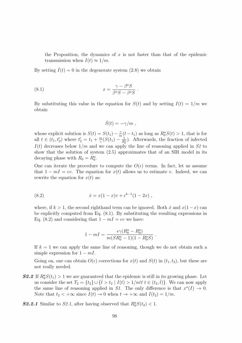
the Proposition, the dynamics of x is not faster than that of the epidemictransmission when I(t) ≈ 1/m.

By setting I(t) = 0 in the degenerate system (2.8) we obtain

(8.1) x =γ − βaS

βnS − βaS.

By substituting this value in the equation for S(t) and by setting I(t) = 1/m weobtain

S(t) = −γ/m ,

whose explicit solution is S(t) = S(t1)− γm(t− t1) as long as Rn

0S(t) > 1, that is forall t ∈ (t1, t

′2) where t′2 = t1 +

mγ(S(t1) − 1

Rn0). Afterwards, the fraction of infected

I(t) decreases below 1/m and we can apply the line of reasoning applied in S1 toshow that the solution of system (2.5) approximates that of an SIR model in itsdecaying phase with R0 = Rn

0 .

One can iterate the procedure to compute the O(ε) terms. In fact, let us assumethat 1 − mI = εv. The equation for x(t) allows us to estimate v. Indeed, we canrewrite the equation for x(t) as:

(8.2) x = x(1− x)v + εk−1(1− 2x) ,

where, if k > 1, the second righthand term can be ignored. Both x and x(1−x) canbe explicitly computed from Eq. (8.1). By substituting the resulting expressions inEq. (8.2) and considering that 1−mI = εv we have:

1−mI =εγ(Rn

0 −Ra0)

m(SRn0 − 1)(1−Ra

0S).

If k = 1 we can apply the same line of reasoning, though we do not obtain such asimple expression for 1−mI.

Going on, one can obtain O(ε) corrections for x(t) and S(t) in (t1, t2), but these arenot really needed.

S2.2 If Ra0S(t1) > 1 we are guaranteed that the epidemic is still in its growing phase. Let

us consider the set T2 = {t2}∪{t > t2 | I(t) > 1/m∀ t ∈ (t2, t)}. We can now applythe same line of reasoning applied in S1. The only difference is that x?(I) → 0.Note that t2 < +∞ since I(t) → 0 when t → +∞ and I(t2) = 1/m.

S2.2.1 Similar to S2.1, after having observed that Ra0S(t2) < 1.

98

S2.2.2 Trivial. �

Lemma 8.1.1. If Rn0 > 1, the set of the solutions of the inequalities 1 < Ra

0 < Rn0 exp{−Ra

0(1−1/Rn

0 )} is non empty.

For fixed values of Rn0 > 1, let us consider the function

hRn0(x) = x−Rn

0 exp{−x(1− 1/Rn0 )} .

We have that hRn0(Rn

0 ) > 0. We are interested to study the sign of the function k(Rn0 ) :=

hRn0(1) = 1 − Rn

0 exp{1/Rn0 − 1}. We have that k(1) = 0, limRn

0→∞ k(Rn0 ) = −∞ and

k(Rn0 ) < 0. It follows that hRn

0(1) < 0 for each Rn

0 > 1. Therefore, it does exist R(Rn0 ) ∈

(1, Rn0 ) such that hRn

0(R) = 0. It follows that choosing Ra

0 with 1 < Ra0 < R(Rn

0 ), wesatisfy the inequality in the thesis. �

Proof of Proposition 2.3.3Let us consider the time interval [0, t1] where t1 is defined in the proof of Prop. 2.3.2.

Since the system is equivalent to a SIR model with R0 = Rn0 , we can employ the SIR

invariant S(t) + I(t) − 1Rn

0logS(t) = const in [0, t1] to compute S1 := S(t1). Since

S(0) = 1 − I0, I(0) = I0 and I(t1) = 1/m it follows that S1 is a zero of the functionf(x) = x+ 1

m− 1

Rn0log x− 1 +O(I0), where O(I0) =

1Rn

0log(1− I0) can be ignored. Since

f(1) = 1/m > 0 and f(1/Rn0 ) = 1/m− Ip < 0 (by hypothesis) it follows that it does exist

S1 such that f(S1) = 0 and

(8.3) S1 ∈ (1/Rn0 , 1)

with lim1/m→0 S1 = 1 and lim1/m→Ip S1 = 1/Rn0 . Since f(x) is increasing for x > 1/Rn

0

the solution is unique.Let us now assume that Ra

0 satisfies the inequalities 1 < Ra0 < Rn

0 exp{−Ra0(1−1/Rn

0 )}(it is possible thanks to lemma 8.1.1), which in particular implies Ra

0 < Rn0 . Since Rn

0 >1/S1 (see Eq. (8.3)), we can distinguish two cases:

• Case 1: Ra0 > 1/S1 ,

• Case 2: Ra0 ≤ 1/S1 .

In Case 2, we have a solution of type C1, satisfying the thesis.Hence, we look only at Case 1. We are guaranteed that the epidemic is still in its

growing phase. Let us consider the time interval [t1, t2] where t2 is defined in the proof ofProp. 2.3.2. Again, we can employ the SIR invariant in [t1, t2] to compute S2 := S(t2).Since S(t1) and I(t1) are known and I(t2) = 1/m it follows that S2 is a non trivial solutionof the equation g(x) = g(S1) where g(x) = x + 1

m− 1

Ra0log x. Function g is convex, has

a absolute minimum for x = 1/Ra0, is strictly decreasing for x < 1/Ra

0 and it is strictly

99

increasing for x > 1/Ra0, limx→0 = +∞ and limx→+∞ = +∞. Since S1 > 1/Ra

0, a uniqueS2 ∈ (0, 1/Ra

0) exists such that g(S2) = g(S1).We now show that S2 > 1/Rn

0 . Since Ra0 < Rn

0 exp{−Ra0(1− 1/Rn

0 )} it follows that:

1− 1

Ra0

log1

Ra0

<1

Rn0

− 1

Ra0

log1

Rn0

.

Since

1− 1

Ra0

log1

Ra0

> S1 −1

Ra0

logS1

we have that g(S2) = g(S1) < g(1/Rn0 ) and thus S2 > 1/Rn

0 since g is decreasing in(0, 1/Ra

0).We have thus demonstrated that Rn

0S2 > 1 which implies that we have a solution oftype C2.

Case 2. Trivially, we have a solution of type C1. �

Lemma 8.1.2. When S(t) = 1/Rn0 , the solution of system (2.5) satisfies I(t) < 1− 1

Rn0+

1Rn

0log 1

Rn0.

Equations of system (2.5) for I and S can be written in the general form{S = −β(t)SI

I = −β(t)SI − γI(8.4)

with β(t) ∈ [βa, βn]. It is easy to show that for system (8.4) the function

S(t) + I(t)− 1

Rn0

logS(t)

is decreasing in t. It follows that

1 = S(0) + I(0)− 1

Rn0

logS(0) > S(t) + I(t)− 1

Rn0

logS(t) .

The thesis follows by substituting S(t) = 1/Rn0 . �

Proof of Proposition 2.3.4Let us define (SSIR(t), ISIR(t)) and (S(t), I(t)) as the fractions of susceptible and

infected individuals for a classical SIR model and for system (2.5), respectively. Inthe phase plane (S, I) the solution of a classical SIR model goes through the point( 1Rn

0, 1 − 1

Rn0+ 1

Rn0log 1

Rn0), corresponding to the epidemic peak. The solutions of system

(2.5) pass through the point (1/Rn0 , I) where I < 1 − 1

Rn0+ 1

Rn0log 1

Rn0thanks to lemma

8.1.2.

100

Let us assume that S∞ < SSIR∞ . It follows that in the phase plane the trajectories

of the two models must intersect at a certain point (S?, I?) with S? < 1/Rn0 . Moreover,

at this point both S and I are decreasing and thus we can assume that the functionsISIR(SSIR) and I(S) are well defined, and that

dISIR

dSSIR(S?) >

dI

dS(S?) .

hence,

−1 +γI?

S?I?βn

> −1 +γI?

S?I?(βnx+ βa(1− x))

which is absurd since βa < βn and x ∈ (0, 1). �

Proof of Proposition 2.3.5Let us consider system (2.5). We have already seen that a time t3 exists such that

I(t3) = 1/m and S(t3) = 1/Rn0 (see Prop. 2.3.2). Moreover, for t > t3 system (2.5) can

be approximated by an SIR model with R0 = Rn0 . Thus we can employ the SIR invariant

in [t3,+∞). It follows that S∞(m) is solution to the equation:

S∞(m)− 1

Rn0

logS∞(m) = S(t3) + I(t3)−1

Rn0

logS(t3) =1

Rn0

+1

m− 1

Rn0

log1

Rn0

while SSIR∞ is solution of the equation

SSIR∞ − 1

Rn0

logSSIR∞ = 1 .

Therefore, we have to compare the solutions of the equations:

l(x) = 1 , l(x) = b(m)

where l(x) = x− 1Rn

0log x and b(m) = 1

Rn0+ 1

m− 1

Rn0log 1

Rn0.

Condition 1/m < Ip implies that b(m) < 1. Function l is convex, has an absoluteminimum at x = 1/Rn

0 with l(1/Rn0 ) < b(m), it is strictly decreasing for x < 1/Rn

0 andlimx→0+ = +∞.

Since we are interested in solutions x < 1/Rn0 , we have that b(m) < 1 implies S∞(m) >

SSIR∞ . Moreover, b(m) is an decreasing function of m and thus S∞(m) is an increasing

function of m.Finally, b(m) ↘ l(1/Rn

0 ) when 1/m → 0; thus S∞(m) → 1/Rn0 when 1/m → 0. �

8.2 Appendix B

8.2.1 The model

The aim here is to introduce a model for a disease transmission process, accounting forheterogeneity with respect to the behaviors adopted spontaneously by the individuals of

101

the host population. The diffusion of the different behaviors performed by the populationis modeled through evolutionary game theory. Specifically, we introduce a simple SIRmodel where individuals can adopt two mutually exclusive behaviors on the basis of theperceived risk of infection through a classical imitation process. We decided to keepthe transmission model as simple as possible. Therefore no latency period, age classes,different levels of symptomaticity, variable viral load over time are considered. The hostpopulation is assumed to be divided into three classes, namely susceptible (S), infective(I) and recovered (R) individuals.

We assume that individuals are able to reduce the force of infection to which theyare exposed as a spontaneous defensive response to the epidemic. Actually, individualsexposed to the risk of infection are only susceptible ones. As we are considering thedynamics of a spontaneous self–protection strategy that reduces the undergoing force ofinfection, neither infective, nor recovered individuals can achieve any benefit through areduction of their force of infection, unless by assuming an altruistic interaction betweenthem and susceptible individuals. Since such investigation is beyond the scope of thiswork, we consider only behavioral changes among susceptible individuals. Therefore,susceptible individuals are divided in two subclasses: individuals adopting a “normal”behavior (Sn) and individuals adopting an “altered” one (Sa), assuming that the latterare able to reduce the received force of infection. From now on, let us denote as bn andba the two different behaviors adopted by Sn and Sa respectively.

Let us define β as the transmission rate, 1/γ the average duration of the infectivityperiod and q ∈ (0, 1) the reduction of the force of infection performed by Sa (e.g., byavoiding crowded environments or by increasing wariness in usual activities involvingcontacts with other individuals). The epidemic flows between classes can be described asfollows:

dSn

dt(t) = −βI(t)Sn(t)

dSa

dt(t) = −qβI(t)Sa(t)

dI

dt(t) = βI(t)[Sn(t) + qSa(t)]− γI(t)

dR

dt(t) = γI(t).

(8.5)

Setting x = Sn/(Sn + Sa), where x represents the fraction of susceptible individualsadopting the normal behavior bn, system (8.5) can be rewritten as follows

102

dS

dt(t) = −β [x(t) + q(1− x(t))]S(t)I(t)

dI

dt(t) = β [x(t) + q(1− x(t))]S(t)I(t)− γI(t)

dR

dt(t) = γI(t)

dx

dt(t) = x(t)(1− x(t)) [qβI(t)− βI(t)] .

(8.6)

where, as mentioned above, S = Sn + Sa is the whole fraction of susceptible individuals.The latter equation of system (8.5), obtained by deriving Sn/(Sn+Sa), can be read as a

“natural” selection process embedded in the transmission dynamics that favors individualsreducing the force of infection.

Let us assume that individuals can also change strategy spontaneously during thecourse of the epidemic, through cost–benefit considerations that involve the perceivedrisk of infection.

This phenomenon perfectly fits to the language of evolutionary game theory, in whichbehaviors correspond to strategies that are adopted or not on the basis of their conve-nience. More specifically here we assume that behavior diffusion is driven by an imitationdynamics [81, 122, 15, 127]: a fraction of the individuals playing strategy bn can switchto strategy ba after having compared the payoffs of the two strategies, namely pn and pa,at a rate proportional to their difference ∆P = pn − pa, with proportionality constantω; conversely for the fraction of the individuals playing ba. As this comparison is basedon the diffusion of information and may not involve only physical contacts between indi-viduals, the imitation process and the pathogen transmission can have two different timescales. Thus let us introduce τ as the time unit for spontaneous behavioral changes, andlet us assume that t = ατ with α ∈ R.

The convenience of two mutually exclusive behaviors is modeled through their cor-responding payoff functions. We consider that all individuals pay a cost for the risk ofinfection, which we assume to depend linearly on the perceived prevalence, M(τ), and itis higher for bn than for ba. Moreover, individuals playing strategy ba pay an extra fixedcost. Hence, the payoffs associated with bn and ba are respectively:

pn(τ) = −mnM(τ)pa(τ) = −k −maM(τ) ,

withmn > ma. We may think ofmn andma as parameters related to the risk of developingsymptoms induced by the two different behaviors bn and ba, while k represents the costof any self-imposable prophylactic measure (e.g., less traveling).

The perceived prevalence M is modeled through an exponentially fading memorymechanism (such as in [48]) as follows:

dM

dt(t) = β [x(t) + q(1− x(t))]S(t)I(t)− θI(t) .

103

where θ weighs the decay of the perceived risk of infection produced by new cases andthus 1/θ can be read as the average duration of the memory of new cases in the perceivedprevalence.

By adding the imitation dynamics in the last equation of system (8.6), the equationfor the fraction of susceptible individuals adopting normal behavior x becomes(8.7)

dx

dt(t) = x(t)(1− x(t)) [qβI(t)− βI(t)] + ω

αx(t)(1− x(t))S [k − (mn −ma)M(t)]

expressed in the time scale of infection transmission process. Equation (8.7) can berewritten in the following form:

dx

dt(t) = x(t)(1− x(t))β(q − 1)I(t) + ρx(t)(1− x(t))S [1−mM(t)] .

where ρ = ωkα, m = (mn −ma)/k.

As a matter of fact, 1/m defines the threshold for the perceived prevalence M(t),over which it is more convenient to adopt the altered behavior. Moreover ρ essentiallyrepresents the speed of the imitation process with respect to the pathogen transmissiondynamics. Finally, q tunes the reduction of the force of infection for individuals adoptingthe altered behavior.

One could consider a more general model for behavior dynamics, including the pos-sibility that individuals can also (rarely) change behavior regardless of cost–benefit con-siderations, as driven by an irrational exploration. This possibility can be modeled as amutation dynamics [81], not favoring any strategy, by considering a mutation rate µ << 1.The resulting equation for x would become

dx

dt(t) = x(t)(1− x(t))β(q − 1)I(t) + ρ[x(t)(1− x(t))S(1−mM(t))− µx+ µ(1− x)] .

Mutation dynamics might be considered to gain more realism (details have been largelydiscussed in [127]). Nonetheless, its effect can be neglected for the purpose of this work.

8.2.2 Sensitivity analysis

In order to assess the robustness of qualitative results shown in the main text, we investi-gate the sensibility of the model by changing one–by–one the values of fitted parametersstarting from the estimates obtained by model fitting.

The timing of the simulated epidemics is highly sensible to changes in the parametervalues, while just slightly differences in the final epidemic size can be appreciated. Ingeneral, the final size varies from 38% to 41% whereas the epidemic peak week can changeof more than 3 weeks.

Results are stable for large values of ρ, representing a fast imitation process, for smallx(0) values, i.e. if altered behavior is initially widespread in the population, and for along lasting memory (Fig. 8.1). As varying x(0) in a range 10−6 − 10−12 does not result

104

ρ

Fin

al e

pide

mic

siz

e

20 30 40 50 60 70 70 100

200

900

38

38.5

39

39.5

40

ρ

Pea

k w

eek

(wee

k of

the

year

)

20 30 40 50 60 7070 100

200

900

42

43

44

45

46

47

1/ θ

Pea

k w

eek

(wee

k of

the

year

)

80 100

120

140

160

180

200

220

240

42

43

44

45

46

47

1/ θ

Fin

al e

pide

mic

siz

e (%

)

80 100

120

140

160

180

200

220

240

39

39.5

40

40.5

41

x(0)

Fin

al e

pide

mic

siz

e (%

)

10−2

10−3

10−4

10−6

10−8

10−1

0

10−1

2

10−1

6

10−2

0

39

39.75

40.5

41.25

42

Weeks (week of the year)

Wee

kly

inci

denc

e(c

ases

per

1,0

00 in

divi

dual

s)

38 39 40 41 42 43 44 45 46 47 48 49 50 510

4

8

12

16

Weeks (week of the year)

Wee

kly

inci

denc

e(c

ases

per

1,0

00 in

divi

dual

s)

38 39 40 41 42 43 44 45 46 47 48 49 50 510

4

8

12

16

x(0)

Pea

k w

eek

(wee

k of

the

year

)

10−2

10−3

10−4

10−6

10−8

10−1

0

10−1

2

10−1

6

10−2

0

42

43

44

45

46

47

Weeks (week of the year)

Wee

kly

inci

denc

e(c

ases

per

1,0

00 in

divi

dual

s)

38 39 40 41 42 43 44 45 46 47 48 49 50 510

4

8

12

16

a b c

d e f

g h i

Figure 8.1: a Final epidemic size as simulated by the proposed model for different valuesof x(0). Other parameters as described in the main text (see Fig. 1). b As is a but forthe peak week. c As is a but for the weekly incidence. Lines colors correspond to pointscolors in a and b. d, e and f As a, b and c but varying ρ. g, h and i As a, b and c butvarying θ.

105

q

Pea

k w

eek

(wee

k of

the

year

)

0.78 0.8

0.82

0.84

0.86

0.88 0.9

0.92

0.94

42

43

44

45

46

47

Weeks (week of the year)

Wee

kly

inci

denc

e(c

ases

per

1,0

00 in

divi

dual

s)

38 39 40 41 42 43 44 45 46 47 48 49 50 510

4

8

12

16

Weeks (week of the year)

Wee

kly

inci

denc

e(c

ases

per

1,0

00 in

divi

dual

s)

38 39 40 41 42 43 44 45 46 47 48 49 50 510

4

8

12

16

Weeks (week of the year)

Wee

kly

inci

denc

e(c

ases

per

1,0

00 in

divi

dual

s)

38 39 40 41 42 43 44 45 46 47 48 49 50 510

4

8

12

16

m

Fin

al e

pide

mic

siz

e (%

)

0.09

6

0.09

7

0.09

8

0.09

9

0.1

0.10

1

0.10

2

0.10

3

0.10

4

38

38.75

39.5

40.25

41

M(0)

Pea

k w

eek

(wee

k of

the

year

)

10.1

10.2

10.3

10.4

10.5

10.6

10.7

10.8

10.9

42

43

44

45

46

47

m

Pea

k w

eek

(wee

k of

the

year

)

0.09

6

0.09

7

0.09

8

0.09

9

0.1

0.10

1

0.10

2

0.10

3

0.10

4

42

43

44

45

46

47

M(0)

Fin

al e

pide

mic

siz

e (%

)

10.1

10.2

10.3

10.4

10.5

10.6

10.7

10.8

10.9

38

39

40

41

q

Fin

al e

pide

mic

siz

e (%

)

0.78 0.8

0.82

0.84

0.86

0.88 0.9

0.92

0.94

39

39.25

39.5

39.75

40a b c

f

g

e

h i

d

Figure 8.2: a Final epidemic size as simulated by the proposed model for different valuesof q. Other parameters as described in the main text (see Fig. 1). b As is a but for thepeak week. c As is a but for the weekly incidence. Lines colors correspond to pointscolors in a and b. d, e and f As a, b and c but varying M(0). g, h and i As a, b and cbut varying m.

106

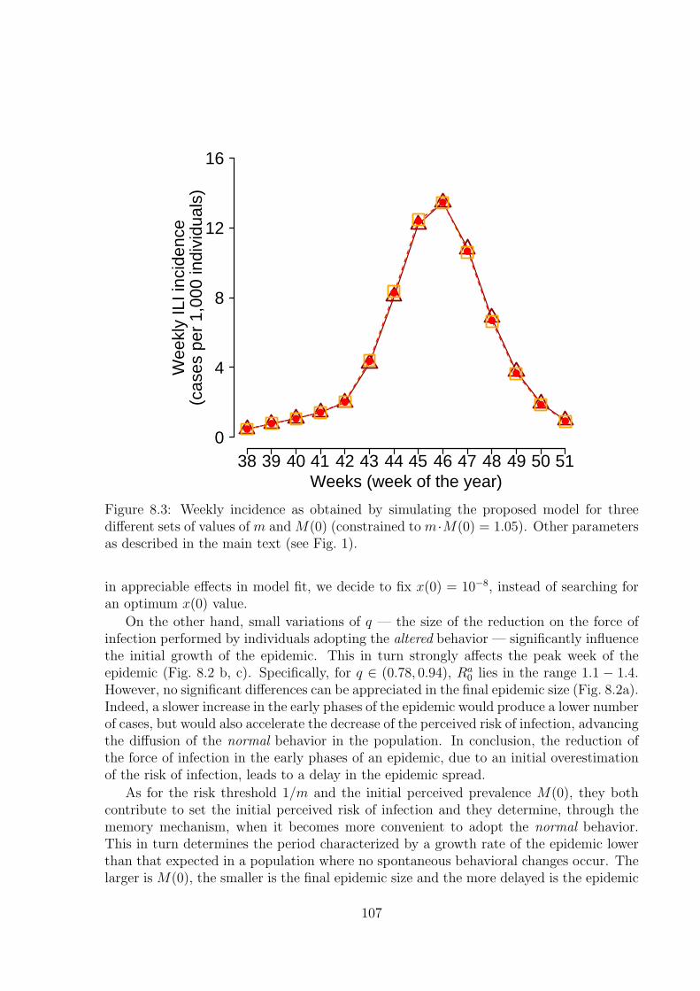
Weeks (week of the year)

Wee

kly

ILI i

ncid

ence

(cas

es p

er 1

,000

indi

vidu

als)

38 39 40 41 42 43 44 45 46 47 48 49 50 510

4

8

12

16

Figure 8.3: Weekly incidence as obtained by simulating the proposed model for threedifferent sets of values of m and M(0) (constrained to m·M(0) = 1.05). Other parametersas described in the main text (see Fig. 1).

in appreciable effects in model fit, we decide to fix x(0) = 10−8, instead of searching foran optimum x(0) value.

On the other hand, small variations of q — the size of the reduction on the force ofinfection performed by individuals adopting the altered behavior — significantly influencethe initial growth of the epidemic. This in turn strongly affects the peak week of theepidemic (Fig. 8.2 b, c). Specifically, for q ∈ (0.78, 0.94), Ra

0 lies in the range 1.1 − 1.4.However, no significant differences can be appreciated in the final epidemic size (Fig. 8.2a).Indeed, a slower increase in the early phases of the epidemic would produce a lower numberof cases, but would also accelerate the decrease of the perceived risk of infection, advancingthe diffusion of the normal behavior in the population. In conclusion, the reduction ofthe force of infection in the early phases of an epidemic, due to an initial overestimationof the risk of infection, leads to a delay in the epidemic spread.

As for the risk threshold 1/m and the initial perceived prevalence M(0), they bothcontribute to set the initial perceived risk of infection and they determine, through thememory mechanism, when it becomes more convenient to adopt the normal behavior.This in turn determines the period characterized by a growth rate of the epidemic lowerthan that expected in a population where no spontaneous behavioral changes occur. Thelarger is M(0), the smaller is the final epidemic size and the more delayed is the epidemic

107

Weeks (week of the year)

Wee

kly

ILI i

ncid

ence

(cas

es p

er 1

,000

indi

vidu

als)

38 39 40 41 42 43 44 45 46 47 48 49 50 510

4

8

12

16

Weeks (week of the year)W

eekl

y IL

I inc

iden

ce(c

ases

per

1,0

00 in

divi

dual

s)

38 39 40 41 42 43 44 45 46 47 48 49 50 51

0

4

8

12

16ba 1/γ=31/γ=2

Figure 8.4: a Weekly ILI incidence as reported to the surveillance system (green) andweekly incidence simulated by the model by assuming 1/γ = 2 days (red). Parametersvalues: β = 0.719, q = 0.83, m = 0.1, ρ = 61.3, µ = 0.005, M(0) = 10.5, x(0) = 10−8,I(0) = 0.00121 and S(0) = 0.1. The estimated basic reproductive number lies in the range1.2 − 1.44 and the reporting factor is 17.9%. b Weekly ILI incidence as reported to thesurveillance system (green) and weekly incidence simulated by the model by assuming1/γ = 3 days (red). Parameters values: β = 0.518, q = 0.84, m = 0.1, ρ = 64.9,µ = 0.005, M(0) = 10.5, x(0) = 10−8, I(0) = 0.00124 and S(0) = 0.1. The estimatedbasic reproductive number lies in the range 1.31− 1.55 and the reporting factor is 15.4%.

peak (see Fig. 8.2 d, e and f). The same is observed for m (see Fig. 8.2 g, h and i).Specifically, variations of the order of 10% in M(0) or in m result in absolute differencesin the epidemic size of about 2% and, most remarkably, in variations of 3-4 weeks of theepidemic peak week.

Actually, the investigated situation is characterized by: (i) a risk of infection unableto sustain the altered behavior as a convenient choice; (ii) an initial overestimation of thisrisk of infection. In this specific case, the product m ·M(0) is the crucial factor (ratherthan the values of the single parameters). In fact, as shown in Fig. 8.3, by varying valuesof m and M(0) under the constraint that their product is kept constant, no appreciabledifferences in model trajectories can be detected.

In our investigation we have assumed a fixed generation time of 2.5 days, accordingto recent estimates [63, 165]. As shown in Fig. 8.4, predictions are not very sensitive tothe length of the generation time (for 1/γ = 2 and 1/γ = 3).

In short, the model is able to account for the notable observed pattern, characterizedby a sudden change in the slope of the incidence, if:

I an initial large diffusion of the altered behavior, due to a perceived risk of infectionover the threshold, occurs;

II the altered behavior results as more convenient for a relevant period of time thanksto a long-lasting memory;

108

III the imitation process is fast enough to allow a sudden change in the distribution ofthe behaviors adopted by the population, which in turn results in a sudden changeof the growth of the epidemic.

In conclusion, m ·M(0) > 1 represents an overestimation of the initial risk of infection.The closer is the product m ·M(0) to one and the larger is ρ, the smaller are the effectsof the overestimation of the risk and thus the shorter is the period characterized by thediffusion of the altered behavior. As a consequence, as this period becomes smaller, thedynamics of the model becomes similar to the one predicted by a “simple” SIR model.

8.2.3 Alert time

Our analysis has revealed that a central role for determining epidemic dynamics has beenplayed by the initial concern about the spread of a new influenza pandemic. Here weinvestigate what would happen if the overestimation of risks occurs at different times(here considered as “alert” times), for example driven by different timing in the massmedia information campaign. Specifically, as shown in Fig. 8.5, if the alert takes placeduring the early phases of the epidemic, no relevant effects are observed in terms of finalepidemic size nor in the peak incidence, while the diffusion of the virus can be sloweddown allowing public health agencies to gain time to perform control strategies such asvaccination (which requires time for the preparation and the distribution of doses). Alertsperformed during the course of the outbreak have limited effects in slowing the epidemicspread and thus they do not allow gaining time for the interventions. However, these alertscan result in lower peak incidence (and thus in a lower burden for health care centers)and in a relevant decline of the final epidemic size. Clearly, alerts performed at the endof the epidemic have no effects on the timing and on the peak incidence of the epidemicsbut may result only in a reduction of the final size as they can contribute to acceleratethe decline of the epidemic.

8.2.4 Analysis of past influenza seasons

As shown in the main text, the proposed model perfectly fits the ILI incidence reportedto the Italian surveillance system during the 2009 H1N1pdm influenza. Specifically, ouranalysis has shown that a self-protection behavior, spontaneously performed by the pop-ulation in response to a high initial perceived risk of infection, represents a plausibleexplanation for the notable observed pattern. As discussed in the main text, this couldhave been induced by the mass media information campaign on the risks of an emerginginfluenza pandemic; such hypothesis is also supported by empirical evidence (such as thetrend of antivirals drugs sales and the sporadic self-imposed school closures during Octo-ber 2009). Our aim in this section is to investigate if behavioral changes spontaneouslyperformed by the population have been a peculiarity of the 2009 pandemic or if (andpossibly how) they could have played a central role during past influenza seasons.

Our analysis focuses on the last three influenza seasons (namely, the 2006-2007, the2007-2008 and the 2008-2009) in Italy and, exactly as for the analysis shown in the main

109

Week

Dai

ly in

cide

nce

(cas

es p

er 1

,000

indi

vidu

als)

1 2 3 4 5 6 7 8 9 10 11 12 13 14 15 16

0

0.4

0.8

1.2

1.6

2

Week of alert

Pea

k da

ily in

cide

nce

1 2 3 4 5 6 7 8 91.2

1.4

1.6

1.8

2

2.2

Week of alertF

inal

epi

dem

ic s

ize

(%)

1 2 3 4 5 6 7 8 934

36

38

40

42

Week of alert

Pea

k w

eek

1 2 3 4 5 6 7 8 97

8

9

10

11b ca

d

Figure 8.5: a Peak week as predicted by the model for different times of the alert. Pa-rameters as in Fig. 1a of the main text, but for M , which is set to 10.5 at the time of thealert (same value as in Fig. 1a of the main text but different time). Horizontal black linerepresents the peak week as predicted by the “classical” SIR model. b Final epidemic sizeas predicted by the model for different times of the alert. Horizontal black line representsthe final epidemic size as predicted by the “classical” SIR model. Parameters as in a. cPeak daily incidence (cases per 1,000 individuals) as predicted by the model for differenttimes of the alert. Horizontal black line represents the peak daily incidence as predictedby the “classical” SIR model. Parameters as in a. d Daily incidence as predicted by themodel for different times of the alert. Colors of the lines correspond to colors of the pointsin a, b and c.

text, it is based on model fit to ILI incidence reported to the Italian surveillance system(data available at http://www.iss.it/iflu/).

We found that considering behavioral dynamics does not improve the accuracy of thefit with respect to a “simple” SIR model for the 2006-2007 and the 2008-2009 influenzaseasons. Specifically, the best parameter sets estimated by using a least square fittingprocedure for both 2006-2007 and 2008-2009 seasons force the system to a configurationcharacterized by the diffusion of a single strategy adopted by the population over thewhole course of the epidemic (i.e., x(t) = 0∀t or x(t) = 1∀t). Therefore, the proposed

110

Weeks (week of the year)

Wee

kly

ILI i

ncid

ence

(cas

es p

er 1

,000

indi

vidu

als)

48 49 50 51 52 1 2 3 4 5 6 7 8 9 10 11 12 13 14

0

2

4

6

8

10

Chr

istm

as h

olid

ays

Weeks (week of the year)

Wee

kly

ILI i

ncid

ence

(cas

es p

er 1

,000

indi

vidu

als)

48 49 50 51 52 1 2 3 4 5 6 7 8 9 10 11 12 13 14

0

2

4

6

8

10

Chr

istm

as h

olid

ays

Weeks (week of the year)

Wee

kly

ILI i

ncid

ence

(cas

es p

er 1

,000

indi

vidu

als)

48 49 50 51 52 1 2 3 4 5 6 7 8 9 10 11 12 13 14

0

2

4

6

8

10

Chr

istm

as h

olid

ays

Weeks (week of the year)

Wee

kly

ILI i

ncid

ence

(cas

es p

er 1

,000

indi

vidu

als)

48 49 50 51 52 1 2 3 4 5 6 7 8 9 10 11 12 13 14

0

2

4

6

8

10

Chr

istm

as h

olid

ays

a b

c d

Figure 8.6: Analysis of the 2006-2007, the 2007-2008 and the 2008-2009 influenza sea-sons. a Weekly ILI incidence as reported to the Italian surveillance system (green) inthe 2006-2007 season and weekly incidence as simulated by the “classical” SIR model(blue). Parameters values: β = 0.49, γ = 0.26, I(0) = 0.001. Since serological analy-sis on those influenza seasons are not available to us, the initial fraction of susceptibleindividuals in the population is S(0) = 0.73 as assumed in literature (e.g., in [105, 28]).The estimated effective reproductive number results to be 1.38 and the reporting factor is15%. b Weekly ILI incidence as reported to the Italian surveillance system (green) in the2008-2009 season and weekly incidence as simulated by the “classical” SIR model (blue).Parameters values: β = 0.46, γ = 0.27, I(0) = 0.001 and S(0) = 0.73. The estimatedeffective reproductive number results to be 1.24 and the reporting factor is 23%. c WeeklyILI incidence as reported to the Italian surveillance system (green) in the 2007-2008 sea-son and weekly incidence as simulated by the proposed model (red). Parameters values:β = 0.35, γ = 0.18, q = 0.89, m = 30, ρ = 400, µ = 0.03, M(0) = 0, x(0) = 0.99,I(0) = 0.001 and S(0) = 0.73. The estimated effective reproductive number lies in therange 1.26− 1.42 and the reporting factor is 26%. d Weekly ILI incidence as reported tothe Italian surveillance system (green) in the 2007-2008 season and weekly incidence assimulated by the “classical” SIR model (blue). Parameters values: β = 0.44, γ = 0.26,I(0) = 0.0001 and S(0) = 0.73. The estimated effective reproductive number results tobe 1.24 and the reporting factor is 27%.

111

Weeks (week of the year)

Wee

kly

inci

denc

e

M(t

)

38 39 40 41 42 43 44 45 46 47 48 49 50 51

0

3

6

9

12

15

0

3

6

9

12

15

Weeks (week of the year)

Wee

kly

inci

denc

e

M(t

)

48 49 50 51 52 1 2 3 4 5 6 7 8 9 10 11 12 13 14

0

2

4

6

8

10

0

0.02

0.04

0.06

0.08

0.1

Chr

istm

as h

olid

ays

ba2007−2008 2009−2010

Figure 8.7: a Weekly incidence (cases per 1,000 individuals) as simulated by the proposedmodel (red) for the 2007-2008 season. Dynamics of the perceived prevalence (gray, scaleon the right axis). Horizontal gray line represents the risk threshold. b As a but for the2009-2010 pandemic season.

model and the “classical” SIR model coincide. Best model fits to the weekly ILI incidencein 2006-2007 and 2008-2009 influenza seasons are shown in Fig. 8.6 a and b.

As regards the 2007-2008 influenza season, we found that the proposed model, ac-counting for behavioral changes in the population, fits the weekly ILI incidence betterthan the “classical” SIR model (see Fig. 8.6 c and d). However, our parameters estimatesuggests no initial overestimation of the perceived prevalence. The diffusion of an “al-tered” behavior could possibly have occurred during the most acute phase of the epidemic,close to the epidemic peak, i.e. when the risk of infection was “really” higher. Hence,even in this case, no overestimation of the perceived risk of infection at the beginningof the epidemic has been detected by our analysis, as opposed to that observed for the2009-2010 season. Fig. 8.7 show the dynamics of the ILI incidence and of the perceivedprevalence, as obtained by fitting the 2009-2010 and the 2007-2008 influenza seasons.

In conclusion, this analysis suggests that behavioral changes would not have playeda relevant role in past influenza seasons, at least in the early stages of the epidemic.The initial overestimation of the risk of infection seems to be a peculiarity of the 2009pandemic.

8.2.5 Analysis of epidemiological and virological surveillance data

By combining virological [88] and epidemiological [87] surveillance data on the 2009–2010 season, we are able to estimate a theoretic lower bound for the weekly number ofH1N1pdm infections. Specifically, we multiply the weekly ILI incidence to the number oflaboratory confirmed cases divided by the number of tested specimens. Tested specimenshave been sampled between the ILI cases identified by physicians participating to thenational surveillance system.

As for the weekly ILI incidence (analyzed in the main text), this different dataset ischaracterized by two distinct exponential growth phases (especially appreciable in the

112

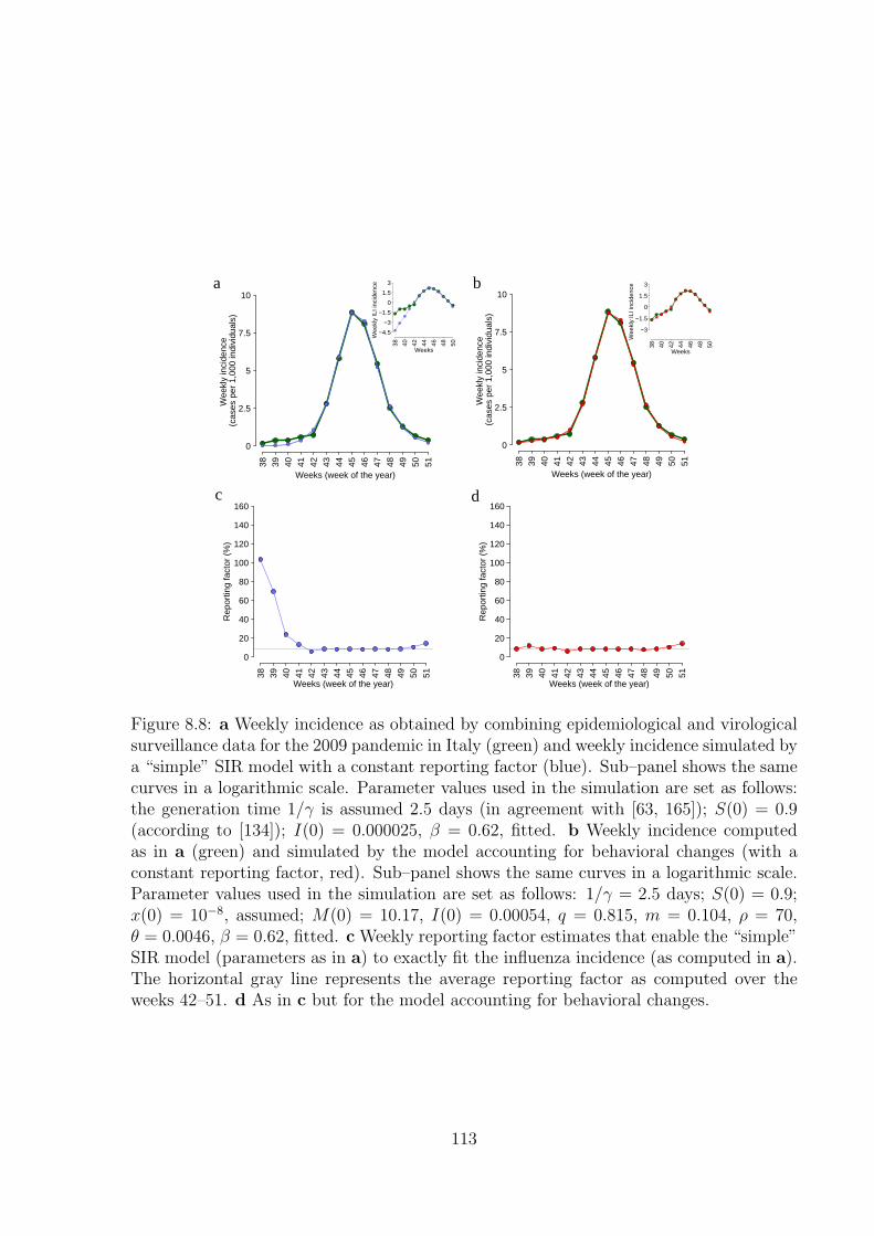
Weeks (week of the year)

Wee

kly

inci

denc

e (c

ases

per

1,0

00 in

divi

dual

s)

38 39 40 41 42 43 44 45 46 47 48 49 50 51

0

2.5

5

7.5

10

Weeks (week of the year)

Rep

ortin

g fa

ctor

(%

)

38 39 40 41 42 43 44 45 46 47 48 49 50 51

0

20

40

60

80

100

120

140

160

Weeks (week of the year)

Rep

ortin

g fa

ctor

(%

)

38 39 40 41 42 43 44 45 46 47 48 49 50 51

0

20

40

60

80

100

120

140

160

Weeks

Wee

kly

ILI i

ncid

ence

38 40 42 44 46 48 50

−4.5

−3

−1.5

0

1.5

3

Weeks (week of the year)W

eekl

y in

cide

nce

(cas

es p

er 1

,000

indi

vidu

als)

38 39 40 41 42 43 44 45 46 47 48 49 50 51

0

2.5

5

7.5

10

Weeks

Wee

kly

ILI i

ncid

ence

38 40 42 44 46 48 50

−3

−1.5

0

1.5

3a b

c d

Figure 8.8: a Weekly incidence as obtained by combining epidemiological and virologicalsurveillance data for the 2009 pandemic in Italy (green) and weekly incidence simulated bya “simple” SIR model with a constant reporting factor (blue). Sub–panel shows the samecurves in a logarithmic scale. Parameter values used in the simulation are set as follows:the generation time 1/γ is assumed 2.5 days (in agreement with [63, 165]); S(0) = 0.9(according to [134]); I(0) = 0.000025, β = 0.62, fitted. b Weekly incidence computedas in a (green) and simulated by the model accounting for behavioral changes (with aconstant reporting factor, red). Sub–panel shows the same curves in a logarithmic scale.Parameter values used in the simulation are set as follows: 1/γ = 2.5 days; S(0) = 0.9;x(0) = 10−8, assumed; M(0) = 10.17, I(0) = 0.00054, q = 0.815, m = 0.104, ρ = 70,θ = 0.0046, β = 0.62, fitted. c Weekly reporting factor estimates that enable the “simple”SIR model (parameters as in a) to exactly fit the influenza incidence (as computed in a).The horizontal gray line represents the average reporting factor as computed over theweeks 42–51. d As in c but for the model accounting for behavioral changes.

113

log scale, see Fig. 8.8a). By fitting a simple SIR model and the proposed model to suchdata, we obtain substantially the same results discussed in the main text: the SIR modelis unable to account for the initial phases of the epidemic, while the model includingbehavioral changes performs much better (see Fig. 8.8a, b).

We found that a simple SIR model with a time dependent reporting factor is ableto capture the initial phase of pandemic only by considering extremely large values ofthe reporting factor (even above 100%, see Fig. 8.8c). Since this new dataset can beinterpreted as a theoretic lower bound for the number of H1N1pdm infections, reportingfactor values above 100% in principle cannot be observable. On the contrary, the modelconsidering behavioral changes does not require such large values for the reporting factor(see Fig. 8.8d). In conclusion, this analysis suggests that a variable reporting factor doesnot seem to be able to explain alone the observed pattern.

8.3 Appendix C

8.3.1 Properties and more details

The biomathematical properties listed in section 3 may be demonstrated as follows:Property A Let us define, to simplify the notation, the parameter:

(8.8) Ψ = kh (Ie) (1− h (Ie)) .

Linearizing at Ee yields the following characteristic polynomial with positive coefficients:

(8.9) λ3 + (Ψ + µ+ βIe)λ2 + ((µ+ βIe)Ψ + (µ+ ν)βIe)λ+ βIe (µ+ ν + µh′ (Ie))Ψ,

for which the Routh-Hurwitz condition yields this inequality in the variable Ψ:(8.10)

RH(Ψ) = (µ+ βIe)Ψ2 +

((µ+ βIe)

2 − βIeµh′ (Ie)+

)Ψ+ (µ+ βIe) βIe(µ+ ν) > 0.

Since the coefficients of power 0 and 2 of eq. (8.10) are positive, and taking also intoaccount the sign of the coefficient of power 1, it is easy to show that if (6.12) holds thenEbeh is LAS.Property B If (6.13) holds then there are two positive values 0 < k1 < k2 such that ifk < k1 or k > k2 then Ebeh is LAS; moreover, if k1 < k < k2 then Ebeh is unstable andk1 and k2 are Hopf points. After some algebra it is easy to verify that at the Hopf pointsthere are Hopf bifurcations since the nonzero speed condition Re

((dλ/dk)|λ=±iωHopf

)6= 0

is fulfilled.Property C As regards the Yabucovitch oscillations, note that: i) the bounded set

A = {(S, I, p) ∈ R+|0 ≤ S + I ≤ 1− h(0), h(0) ≤ p ≤ 1}

is positively invariant and attractive; ii) Ebeh is unstable, and Edfe, which is in the bound-ary of A, has as the stable manifold the line (w, 0, 1) w ∈ [0, 1] to which Ebeh does not

114

belong, excluding heterocline orbits. Thus we may apply the Yabucovitch theorem.Property D Since asymptotically p(t) ≥ h(0), it follows that for large times:

S ′ ≤ µ (1− h(0)− S) ,

i.e. asymptotically S(t) ≤ (1− h(0)). This in turn implies:

I ′ ≤ βI(1− h(0)−R−1

0

)= β (pc − h(0)) I.

Thus, if h(0) > pc then I(t) → 0 implying p(t) → h(0) and S(t) → 1 − h(0), i.e. Edfe isGAS.Let us now discuss the case of an exponentially fading memory in the perceived risk ofvaccination with linear h(I) = ϑI. The Routh-Hurwitz stability condition reads:

(8.11) G(Ψ, b) = c2(b)Ψ2 + c1(b)Ψ + c0(b) > 0

where Ψ is as in eq. (8.8), and the coefficients are third order polynomials in the delayparameter b. Thus, for each b there are at most two bifurcation values for k, whereas foreach k there may be at most three bifurcation values for b.

115

116

Bibliography

[1] F. R. Adler and J. M. Losada. Adaptive Dynamics of Infectious Diseases: In Pursuitof Virulence Management. Cambridge University Press, 2002.

[2] A. Ahituv, V. J. Hotz, and T. Philipson. The Responsiveness of the Demand forCondoms to the Local Prevalence of AIDS. J Hum Resour, 31(4):869–897, 1996.

[3] M. Ajelli, M. Iannelli, P. Manfredi, and M. L. Ciofi degli Atti. Basic mathematicalmodels for the temporal dynamics of HAV in medium-endemicity Italian areas.Vaccine, 26(13):1697–1707, 2008.

[4] M. Ajelli, S. Merler, A. Pugliese, and C. Rizzo. Model predictions and evaluationof possible control strategies for the 2009 A/H1N1v influenza pandemic in Italy.Epidemiol Infect, Published Online by Cambridge University Press 14 June 2010,2010.

[5] R. M. Anderson and R. M. May. Infectious diseases of humans: dynamics andcontrol. Oxford, UK: Oxford University Press, 1991.

[6] R. M. Anderson and R. M. May. Infectious diseases of humans: dynamics andcontrol. Oxford, UK: Oxford University Pres, 1992.

[7] V. Andreasen, J. Lin, and S. Levin. The dynamics of cocirculating influenza strainsconferring partial cross-immunity. J Math Biol, 35(7):825–842, 1997.

[8] D. A. Asch, J. Baron, J. C. Hershey, H. Kunreuther, J. Meszaros, I. Ritov, andM. Spranca. Omission bias and pertussis vaccination. Medical Decision Making,14(2):118–23, 1994.

[9] F. Bagnoli, P. Lio, and L. Sguanci. Risk perception in epidemic modeling. PhysRev E, 76(6):061904–061911, 2007.

[10] M. Baguelin, A. J. V. Hoek, M. Jit, S. Flasche, P. J. White, and W. J. Edmunds.Vaccination against pandemic influenza A/H1N1v in England: A real-time economicevaluation. Vaccine, 28(12):2370–2384, 2010.

[11] D. Balcan, V. Colizza, B. Goncalves, H. Hu, J. J. Ramasco, and A. Vespignani.Multiscale mobility networks and the spatial spreading of infectious diseases. ProcNatl Acad Sci USA, 106(51):21484–21489, 2009.

117

[12] D. Balcan, H. Hu, B. Goncalves, P. Bajardi, C. Poletto, J. J. Ramasco, D. Paolotti,N. Perra, M. Tizzoni, W. V. Broeck, V. Colizza, and A. Vespignani. Seasonaltransmission potential and activity peaks of the new influenza A (H 1 N 1): aMonte Carlo likelihood analysis based on human mobility. BMC Med, 7(1):45,2009.

[13] S. Barrett. Global disease eradication. Journal of European Economic Association,1(2,3):591–600, 2003.

[14] S. Basu, G. B. Chapman, and A. P. Galvani. Integrating epidemiology, psychol-ogy, and economics to achieve HPV vaccination targets. Proc Natl Acad Sci USA,105:19018–19023, 2008.

[15] C. T. Bauch. Imitation dynamics predict vaccinating behaviour. Proc R Soc B,27:1669–1675, 2005.

[16] C. T. Bauch and D. J. D. Earn. Vaccination and the theory of games. Proc NatlAcad Sci USA, 101:13391–13394, 2004.

[17] C. T. Bauch, A. P. Galvani, and D. J. D. Earn. Group interest versus self-interest insmallpox vaccination policy. Proc Natl Acad Sci USA, 100(18):10564–10567, 2003.

[18] H. Bedford and M. Lansley. More vaccines for children? Parents’ views. MVaccine,25:7818–7823, 2007.

[19] S. Bonhoeffer and M. A. Nowak. Mutation and the evolution of virulence. Proc RSoc B, 258:133–140, 1994.

[20] M. Boni, J. Gog, V. Andreasen, and F. Christiansen. Influenza drift and epidemicsize: the race between generating and escaping immunity. Theor Popul Biol, 65:179–191, 2004.

[21] M. C. J. Bootsma and N. M. Ferguson. The effect of public health measures on the1918 influenza pandemic in US cities. Proc Natl Acad Sci USA, 104(18):7588–7593,2007.

[22] R. Breban, R.and Vardavas and S. Blower. Mean-field analysis of an inductivereasoning game: Application to influenza vaccination. Phys Rev E, 76(3):031127,2007.

[23] D. L. Brito, E. Sheshinski, and M. D. Intriligator. Externalities and compulsoryvaccinations. Journal of Public Economics, 45:69–90, 1991.

[24] G. L. Campbell and J. M. Hughes. Plague in India: A New Warning from an OldNemesis. Ann Intern Med, 122(2):151–153, 1995.

[25] V. Capasso and G. Serio. A generalization of the Kermack-McKendrick deterministicepidemic model. Mathematical Biosciences, 42(1-2):43–61, 1978.

118

[26] C. Castillo-Chavez, H. Hethcote, V. Andreasen, S. A. Levin, and W. M. Liu. Epi-demiological models with age structure, proportionate mixing, and cross-immunity.J Math Biol, 89(27):233–258, 1989.

[27] S. Cauchemez, C. Ferguson, N. M.and Wachtel, A. Tegnell, G. Saour, B. Duncan,and A. Nicoll. Closure of schools during an infuenza pandemic. Lancet, 9:473–481,2009.

[28] S. Cauchemez, A. Valleron, P. Boelle, A. Flahault, and N. M. Ferguson. Estimatingthe impact of school closure on influenza transmission from Sentinel data. Nature,452:750 – 754, 2007.

[29] F. H. Chen. A Susceptible-infected Epidemic Model with Voluntary Vaccinations .J Math Biol, 53(2):253–272, 2006.

[30] R. T. Chen and W. A. Orenstein. Epidemiologic Methods in Immunization Pro-grams. Epidemiologic Reviews, 18(2):99–117, 1996.

[31] G. Chowell, C. E. Ammon, N. W. Hengartner, and J. M Hyman. Estimation of thereproductive number of the spanish flu epidemic in geneva, switzerland. Vaccine,24:p6747–6750, 2006.

[32] G. Chowell, C. E. Ammon, N. W. Hengartner, and J. M. Hyman. Transmissiondynamics of the great influenza pandemic of 1918 in geneva, switzerland: Assessingthe effects of hypothetical interventions. J Theor Biol, 241:193–204, 2006.

[33] M. L. Ciofi degli Atti, S. Merler, C. Rizzo, M. Ajelli, M. Massari, P. Manfredi,C. Furlanello, G. Scalia Tomba, and M. Iannelli. Mitigation measures for pandemicinfluenza in Italy: an individual based model considering different scenarios. PLoSONE, 3(3):e1790, 2008.

[34] C.T. Codeco, P.M. Luz, F. Coelho, A.P. Galvani, and C. Struchiner. Vaccinatingin disease-free regions: a vaccine model with application to yellow fever. J R SocInterface, 4(17):1742–5689, 2007.

[35] S. Cohuet, A. Bukasa, R Heathcock, J. White, K. Brown, M. Ramsay, and G. Fraser.A measles outbreak in the Irish traveller ethnic group after attending a funeral inEngland, March–June 2007. Epidemiol and Infect, 12:1–7, 2009.

[36] M. G. Cojocaru, C. T. Bauch, and M. D. Johnston. Dynamics of vaccination strate-gies via projected dynamical systems. Bulletin of Mathematical Biology, 69:1453–1476, 2007.

[37] V. Colizza, A. Barrat, M. Barthelemy, A.-J. Valleron, and A. Vespignani. Mod-eling the worldwide spread of pandemic influenza: baseline case and containmentinterventions. PLoS Med, 4(1):e13, 2007.

119

[38] V. Colizza, A. Barrat, M. Barthelemy, and A. Vespignani. The role of the airlinetransportation network in the prediction and predictability of global epidemics. ProcNatl Acad Sci USA, 103(7):2015–2020, 2006.

[39] B.J. Cowling, DM Ng, DK Ip, Q. Liao, WW Lam, J.T. Wu, JT Lau, S.M. Griffiths,and R. Fielding. Community Psychological and Behavioral Responses through theFirst Wave of the 2009 Influenza A (H1N1) Pandemic in Hong Kong. J Infect Dis,202(6):867–876, 2010.

[40] A. W. Crosby. America’s forgotten pandemic: the influenza of 1918. Cambridge,UK: Cambridge University Press, 1990.

[41] V. J. Davey, R. J. Glass, H. J. Min, W. E. Beyeler, and L. M. Glass. Effective, robustdesign of community mitigation for pandemic influenza: a systematic examinationof proposed US guidance. PLoS ONE, 3(7):e2606, 2008.

[42] S. Del Valle, H. Hethcote, J. M. Hyman, and C. Castillo-Chavez. Effects of behav-ioral changes in a smallpox attack model. Math Biosci, 195(2):228–251, 2005.

[43] Istituto Superiore di Sanita. Surveillance of adverse events, 1999.

[44] O. Diekmann, J. A. P Heesterbeek, and J. A. J. Metz. On the definition and thecomputation of the basic reproduction ratio R0 in models for infectious diseases inheterogeneous populations. J Math Biol, 28(4):365–382, 1990.

[45] A. d’Onofrio and P. Manfredi. Information-related changes in contact patterns maytrigger oscillations in the endemic prevalence of infectious diseases. J Theor Biol,256(3):473–478, 2008.

[46] A. d’Onofrio and P. Manfredi. Vaccine demand driven by vaccine side effects: dy-namic implications for SIR diseases. J Theor Biol, 264:237–252, 2010.

[47] A. d’Onofrio, P. Manfredi, and E. Salinelli. Bifurcation threshold in an SIR modelwith information dependent vaccination. Mathematical Modelling of Natural Phe-nomena, 2:323–38, 2007.

[48] A. d’Onofrio, P. Manfredi, and E. Salinelli. Vaccinating behaviour, information, andthe dynamics of SIR vaccine preventable diseases. Theor Popul Biol, 71(3):301–317,2007.

[49] A. d’Onofrio, P. Manfredi, and E. Salinelli. Fatal SIR diseases and rational exemp-tion to vaccination. Mathematical Medicine and Biology, 25(4):337–357, 2008.

[50] K. T. D. Eames. Networks of influence and infection: parental choices and childhooddisease. J R Soc Interface, 6(38):811–814, 2009.

120

[51] D. Edwards, J. C. Man, P. Brand, J. P. Katsra, K. Sommerer, H. A. Stone,E. Nardell, and G. Scheuch. Inhaling to mitigate exhaled bioaerosols. Proc NatlAcad Sci USA, 101(50):17383–17388, 2004.

[52] J. M. Epstein. Modelling to contain pandemics. Nature, 460(7256):687, 2009.

[53] J. M. Epstein, J. Parker, D. Cummings, and R. A. Hammond. Coupled contagiondynamics of fear and disease: mathematical and computational explorations. PLoSOne, 3(12):e3955, 2008.

[54] European Commission. Organisation of school time in Europe, Primary and generalsecondary education, 2009/10 school year, 2009.

[55] D. Farchy. A common good: whither the global eradication of the measles virus.Working Paper World Bank, 2006.

[56] N. Ferguson. Capturing human behaviour. Nature, 446(7137):733, 2007.

[57] N. M. Ferguson, D. A. Cummings, S. Cauchemez, C. Fraser, S. Riley, A. Meeyai,S. Iamsirithaworn, and D. S. Burke. Strategies for containing an emerging influenzapandemic in Southeast Asia. Nature, 437(7056):209–214, 2005.

[58] N. M. Ferguson, D. A. Cummings, C. Fraser, J. C. Cajka, and P. C. Cooley. Strate-gies for mitigating an influenza pandemic. Nature, 442(7101):448–452, 2006.

[59] N. M. Ferguson, D. A. Cummings, C. Fraser, J. C. Cajka, P. C. Cooley, and D. S.Burke. Strategies for mitigating an influenza pandemic. Nature, 442:448–452, 2006.

[60] A. Ferro, S. Cinquetti, T. Menegon, G. Napoletano, L. Bertoncello, and M. Valsec-chi. Overcoming mandatory vaccination policy: first steps. Annali di Igiene, 20:3–8,2008.

[61] P. E. M. Fine and J. A. Clarkson. Individual versus public priorities in the deter-mination of optimal vaccination policies. Am J Epidemiol, 124:1012–1020, 1986.

[62] Center for Disease Control. Vaccine safety, 1999.

[63] C. Fraser, C. A. Donnelly, S. Cauchemez, W. P. Hanage, M. D. Van Kerkhove, T. D.Hollingsworth, J. Griffin, R. F. Baggaley, H. E. Jenkins, E. J. Lyons, T. Jombart,W. R. Hinsley, N. C. Grassly, F. Balloux, A. C. Ghani, N. M. Ferguson, A. Ram-baut, O. G. Pybus, H. Lopez-Gatell, C. M. Alpuche-Aranda, I. Bojorquez Chapela,E. Palacios Zavala, D. M. Espejo Guevara, F. Checchi, E. Garcia, S. Hugonnet,C. Roth, and The WHO Rapid Pandemic Assessment Collaboration. Pandemic Po-tential of a Strain of Influenza A (H1N1) : Early Findings. Science, 324(5934):1557–1561, 2009.

121

[64] V. Friederichs, J. C. Cameron, and Robertson C. Impact of adverse publicity onMMR vaccine uptake: a population based analysis of vaccine uptake records for onemillion children, born 1987–2004. Arch. Diseases Childood, 91(6):465–468, 2006.

[65] K. Frost, E. Frank, and E. Maibach. Relative risk in the news media: a quantificationof misrepresentation. American Journal of Public Health, 87(5):842–845, 1997.

[66] S. Funk, E. Gilad, and V. A. A. Jansen. Endemic disease, awareness, and localbehavioural response. J Theor Biol, 264(2):501–509, 2010.

[67] S. Funk, E. Gilad, C. Watkins, and V. A. A. Jansen. The spread of awareness andits impact on epidemic outbreaks. Proc Natl Acad Sci USA, 106(16):6872–6877,2009.

[68] S. Funk, M. Salathe, and V. A. A. Jansen. Modelling the influence of human be-haviour on the spread of infectious diseases: a review. J R Soc Interface, 7(50):1247–1256, 2010.

[69] A. P. Galvani, T. C. Reluga, and G. B. Chapman. Long-standing influenza vacci-nation policy is in accord with individual self-interest but not with the utilitarianoptimum. Proc Natl Acad Sci USA, 104(13):5692–5697, 2007.

[70] E. J. Gangarosa, A. M. Galazka, C. R. Wolfe, R. E. Phillips, L. M. Gangarosa,Miller E., and R. T. Chen. Impact of anti-vaccine movements on pertussis control:the untold story. Lancet, 351:356–61, 1998.

[71] G. P. Garnett and R. M. Anderson. Sexually transmitted diseases and sexual be-havior: insights from mathematical models. J Infect Dis, 174:150–161, 1996.

[72] P.Y. Geoffard and T. Philipson. Disease eradication: private versus public vaccina-tion. Am Econ Rev, 87:222–230, 1997.

[73] T. C. Germann, K. Kadau, I. M. J. Longini, and C. A. Macken. Mitigation strategiesfor pandemic influenza in the United States. Proc Natl Acad Sci USA, 103(15):5935–5940, 2006.

[74] A. C. Ghani, M. Baguelin, J. Griffin, S. Flasche, A. J. Van Hoek, S. Cauchemez,C. Donnelly, C. Robertson, M White, J Truscott, C Fraser, T Garske, P White,S Leach, I Hall, H Jenkins, N Ferguson, and B Cooper. The early transmissiondynamics of H1N1pdm influenza in the United Kingdom. PLoS Curr Influenza,2:RRN1130, 2009.

[75] M. Z. Gojovic, B. Sander, D. Fisman, M. D. Krahn, and C. T. Bauch. Modellingmitigation strategies for pandemic (H1N1) 2009. Can Med Assoc J, 181(10):673–680, 2009.

122

[76] M. C. Gonzalez, C. A. Hidalgo, and A. L. Barabasi. Understanding individualhuman mobility patterns. Nature, 453(7196):779–782, 2008.

[77] T. Gross, C. J. D. D’Lima, and B. Blasius. Epidemic Dynamics on an AdaptiveNetwork. Phys Rev Lett, 96(20):208701, 2006.

[78] M. E. Halloran, N. M. Ferguson, S. Eubank, I. M. Longini Jr, D. A. T. Cummings,B. Lewis, S. Xu, C. Fraser, A. Vullikanti, T. C. Germann, D. Wagener, R. Beckman,K. Kadau, C. Barrett, C. A. Macken, D. S. Burke, and P. Cooley. Modeling targetedlayered containment of an influenza pandemic in the United States. Proc Natl AcadSci USA, 105(12):4639–4645, 2008.

[79] B. Hanratty, O Holt, E. Duffell, W. Patterson, J. M. Ramsay, M. White, and P. Jin,L.and Litton. UK measles outbreak in non-immune anthroposophic communities:the implications for the elimination of measles from Europe. Epidemiol Infect,125:377–383, 2000.

[80] R. J. Hatchett, C. E. Mecher, and M. Lipsitch. Public health interventions andepidemic intensity during the 1918 influenza pandemic. Proc Natl Acad Sci USA,104(18):7582–7587, 2007.

[81] J. Hofbauer and K. Sigmund. Evolutionary Games and Population Dynamics. Cam-bridge University Press, 1998.

[82] S. Holly, H. Anita, M.L. Mary-Louise, W. Kirsten, L. Chris, V. Debbie, and M. I. C.Raina. Why do I need it? I am not at risk! Public perceptions towards the pandemic(H1N1) 2009 vaccine. BMC Infect Dis, 10:1471–2334, 2010.

[83] F. Hoppensteadt. Singular Perturbations on the Infinite Interval. Transactions ofthe American Mathematical Society, 123:521–535, 1966.

[84] L. Hufnagel, D. Brockmann, and T. Geisel. Forecast and control of epidemics in aglobalized world. Proc Natl Acad Sci USA, 101(42):15124–15129, 2004.

[85] Istituto Superiore di Sanita. FluNews Aggiornamento epidemiologico settimanalenumero 14, 25-31 January 2010., 2010. (In Italian).

[86] Istituto Superiore di Sanita. FluNews Aggiornamento epidemiologico settimanalenumero 22, 22-28 March 2010., 2010. (In Italian).

[87] Istituto Superiore di Sanita. Stagione influenzale 2009/2010: Sorveglianza epidemi-ologica, 2010. (Available in Italian at http://www.iss.it/iflu/risu/cont.php?id=141&lang=1&tipo=5).

[88] Italian Ministry of Health. Sorveglianza virologica dell’influenza, 2010. (Avail-able in Italian at http://www.nuovainfluenza.salute.gov.it/nuovainfluenza/andamentoEpidemiaNuovaInfluenza.jsp?id=1223).

123

[89] V. A. A. Jansen, N. Stollenwerk, H. J. Jensen, M. E. Ramsay, W. J. Edmunds, andC. J. Rhodes. Measles Outbreaks in a Population with Declining Vaccine Uptake.Science, 301(5634):804, 2003.

[90] J. H. Jones and M. Salathe. Early assessment of anxiety and behavioral responseto novel swine-origin influenza A (H1N1). PloS One, 4:e8032, 2009.

[91] R.E. Kasperson, O. Renn, P. Slovic, H.S. Brown, J. Emel, R. Goble, J.X. Kasperson,and S. Ratick. The social amplification of risk: A conceptual framework. Riskanalysis, 8(2):177–187, 1988.

[92] M. J. Keeling, M. E. J. Woolhouse, R. M. May, G. Davies, and B. T. Grenfell. Mod-elling vaccination strategies against foot-and-mouth disease. Nature, 421(6919):136–142, 2002.

[93] I. Z. Kiss, J. Cassell, M. Recker, and P. L. Simon. The impact of informationtransmission on epidemic outbreaks. Math Biosci, 225(1):1–10, 2010.

[94] La Repubblica (National newspaper). Caso sospetto di influenza A la scuolachiude per 2 giorni (September 29, 2009), 2009. (In Italian, article avail-able at http://ricerca.repubblica.it/repubblica/archivio/repubblica/

2009/09/29/caso-sospetto-di-influenza-la-scuola-chiude.html).

[95] La Repubblica (National newspaper). Davanti a scuola sorpresa e paurama c’e pure chi brinda alla vacanza (October 9, 2009), 2009. (In Ital-ian, article available at http://ricerca.repubblica.it/repubblica/archivio/repubblica/2009/10/09/davanti-scuola-sorpresa-paura-ma-pure.html).

[96] La Repubblica (National newspaper). Influenza: un caso di virusA scuola chiusa, riapre oggi, 2009. (In Italian, article available athttp://ricerca.repubblica.it/repubblica/archivio/repubblica/2009/

10/06/influenza-un-caso-di-virus-scuola-chiusa.html).

[97] La Repubblica (National newspaper). Virus A, chiusa scuola aPomigliano (October 4, 2009), 2009. (In Italian, article available athttp://ricerca.repubblica.it/repubblica/archivio/repubblica/2009/

10/04/virus-chiusa-scuola-pomigliano.html).

[98] JT Lau, H. Tsui, M. Lau, and X. Yang. SARS transmission, risk factors, andprevention in Hong Kong. Emerg Infect Dis, 10(4):587–92, 2004.

[99] B. Y. Lee, S. T. Brown, G. Korch, P. C. Cooley, R. K. Zimmerman, W. D. Wheaton,S. M. Zimmer, J. J. Grefenstette, R. R. Bailey, T. M. Assi, and Burke D. S. Acomputer simulation of vaccine prioritization, allocation, and rationing during the2009 H1N1 influenza pandemic. Vaccine, 28(31):4875–4879, 2010.

124

[100] W. Liu, H. W. Hethcote, and S. A. Levin. Dynamical behavior of epidemiologicalmodels with nonlinear incidence rates . J Math Biol, 25(4):359–380, 1987.

[101] W. Liu, S. A. Levin, and Y. Iwasa. Influence of nonlinear incidence rates upon thebehavior of SIRS epidemiological models. J Math Biol, 23(2):187–204, 1986.

[102] J. O. Lloyd-Smith, S. J. Schreiber, P. E. Koop, and W. M. Getz. Superspreadingand the effect of individual variation on disease emergence. Nature, 438:355–359,2005.

[103] I. M. J. Longini, M. E. Halloran, A. Nizam, and Y. Yang. Containing PandemicInfluenza with Antiviral Agents. Am J Epidemiol, 159(7):623–633, 2004.

[104] I. M. J. Longini, A. Nizam, S. Xu, K. Ungchusak, W. Hanshaoworakul, D. A.Cummings, and M. E. Halloran. Containing pandemic influenza at the source.Science, 309(5737):1083–1087, 2005.

[105] Jr I. M. Longini, J. S. Koopman, M. Haber, and G. A. Cotsonis. Statistical in-ference for infectious diseases: risk-specific household and community transmissionparameters. Am J Epidemiol, 128(4):845–859, 1988.

[106] E. T. Luman, Fiore A. E., Strine T. W., and L. E. Barker. Impact of thimerosal-related changes in hepatitis B vaccine, birth-dose recommendations. J. AmericanMedical Association, 291:2351–2358, 2004.

[107] A. Maayan-Metzger, P. Kedem-Friedrich, and J. Kuint. To vaccinate or not tovaccinate: that is the question: why are some mothers opposed to giving theirinfants hepatitis B vaccine? Vaccine, 23:1941–1948, 2004.

[108] P. Manfredi, A. D’Onofrio, P. della Posta, and E. Salinelli. Rational exemption tovaccination: from dynamics to behaviour. Epidemics Conference, Asilomar (CA),December 2009.

[109] P. Manfredi, P. D. Posta, A. d’Onofrio, E. Salinelli, F. Centrone, C. Meo, andP. Poletti. Optimal vaccination choice, vaccination games, and rational exemption:An appraisal. Vaccine, 28(1):98–109, 2009.

[110] A. Mas Colell and M. D. Whinston. Microeconomic theory. Oxford, UK: OxfordUniversity Press, 1995.

[111] R.M. May and M.A. Nowak. Coinfection and the evolution of parasite virulence.Proceedings: Biological Sciences, 261(1361):209–215, 1995.

[112] S. Merler and M. Ajelli. The role of population heterogeneity and human mobilityin the spread of pandemic influenza. Proc R Soc B, 277(1681):557–565, 2010.

[113] S. Merler, M. Ajelli, and C. Rizzo. Age-prioritized use of antivirals during aninfluenza pandemic. BMC Infect Dis, 9:117, 2009.

125

[114] S. Merler, P. Poletti, M. Ajelli, B. Caprile, and P. Manfredi. Coinfection can triggermultiple pandemic waves. J Theor Biol, 254(2):499–507, 2008.

[115] C. E. Mills, J. M. Robins, and M. Lipsitch. Transmissibility of 1918 pandemicinfluenza. Nature, 432:904–906, 2004.

[116] V. Molina and Y. Shoenfeld. Infection, vaccines and other environmental triggersof autoimmunity. Autoimmunity, 38:235–245, 2005.

[117] I. A. Moneim. The effect of using different types of periodic contact rate on thebehaviour of infectious diseases: A simulation study. Computers in Biology andMedicine, 37, 2007.

[118] C. V. Munayco, J. Gomez, V. A. Laguna-Torres, J. Arrasco, TJ Kochel, V. Fiestas,J. Garcia, J. Perez, I. Torres, F. Condori, H. Nishiura, and G. Chowell. Epidemio-logical and transmissibility analysis of influenza a (h1n1) v in a southern hemispheresetting: Peru. Eurosurveill, 14:pii: 19299, 2009.

[119] K. M. Neuzil, C. Hohlbein, and Y. Zhu. Illness among schoolchildren during in-fluenza season: effect on school absenteeism, parental absenteeism from work, andsecondary illness in families. Arch Pediatr Adolesc Med, 156(10):986–991, 2002.

[120] A. Nicoll, D. Elliman, and E. Ross. MMR vaccination and autism 1998. Br med J,316:715–716, 1998.

[121] H. Nishiura. Time variations in the transmissibility of pandemic influenza in Prussia,Germany, from 1918-19. Theoretical Biology and Medical Modelling, 4:20, 2007.

[122] M. A. Nowak and K. Sigmund. Evolutionary Dynamics of Biological Games. Science,303:793–799, 2004.

[123] R.E. O’Malley Jr. Singular perturbation methods for ordinary differential equations.Springer-Verlag, 1991.

[124] A. Perisic and C. T. Bauch. Social contact networks and disease eradicability undervoluntary vaccination. PLoS Comp Biol, 5(2):e1000280, 2009.

[125] T. Philipwon. Private Vaccination and Public Health: An Empirical Examinationfor U.S. Measles. J Hum Resour, 31(3):611–630, 1996.

[126] S. Plotkin. Lessons learned concerning vaccine safety. Vaccine, 20(Suppl. 1):S16–S19, 2002.

[127] P. Poletti, B. Caprile, M. Ajelli, A. Pugliese, and S. Merler. Spontaneous behaviouralchanges in response to epidemics. J Theor Biol, 260(1):31–40, 2009.

126

[128] A. M. Presanis, D. De Angelis, The New York City Swine Flu Investigation Team,A. Hagy, C. Reed, S. Riley, B. S. Cooper, L. Finelli, P. Biedrzycki, and M. Lipsitch.The Severity of Pandemic H1N1 Influenza in the United States, from April to July2009: A Bayesian Analysis. PLoS Med, 6(12):e1000207, 2009.

[129] T. C. Reluga. An SIS epidemiology game with two subpopulations. Journal ofBiological Dynamics, 200:1–19, 2008.

[130] T. C. Reluga. Game theory of social distancing in response to an epidemic. PLoSComp Biol, 6(5):e1000793, 2010.

[131] T. C. Reluga, C. T. Bauch, and A. P. Galvani. Evolving public perceptions andstability in vaccine uptake. Mathematical Biosciences, 204(2):185–198, 2006.

[132] S. Riley, C. Fraser, C. A. Donnelly, A. C. Ghani, L. J. Abu-Raddad, A. J. Hedley,G. M. Leung, L. Ho, T. Lam, T. Q. Thach, K. Chau, P. Chan, S. Lo, T. Leung,P. Tsang, W. Ho, K. Lee, E. M. C. Lau, N. M. Ferguson, and R. M. Anderson.Transmission Dynamics of the Etiological Agent of SARS in Hong Kong: Impact ofPublic Health Interventions. Science, 300(5627):1961 – 1966, 2003.

[133] S. Risau-Gusman and D. H. Zanette. Contact switching as a control strategy forepidemic outbreaks. arXiv[q-bio.PE]:0806.1872, 2008.

[134] C. Rizzo, M. C. Rota, A. Bella, V. Alfonsi, S. Declich, M. G. Caporali, A. Ranghi-asci, G. Lapini, S. Piccirella, S. Salmaso, and E Montomoli. Cross-reactive antibodyresponses to the 2009 A/H1N1v influenza virus in the Italian population in the pre-pandemic period. Vaccine, 28(10):3558–3562, 2010.

[135] R. J. Roberts, Q. D. Sandifer, Evans M. R., Nolan-Farrell M. Z., and Davis P. M.Reasons for non-uptake of measles, mumps and rubella catch up immunisation in ameasles epidemic and side effects of the vaccine. British Medical Journal, 310:1629–1639, 1995.

[136] G. J. Rubin, R. Amlot, L. Page, and S. Wessely. Public perceptions, anxiety, andbehaviour change in relation to the swine flu outbreak: cross sectional telephonesurvey. Br Med J, 339:b2651, 2009.

[137] M. Z. Sadique, W. J. Edmunds, R. D. Smith, W. J. Meerding, O. de Zwart, J. Brug,and P. Beutels. Precautionary behavior in response to perceived threat of pandemicinfluenza. Emerg Infect Dis, 13(9):1307–1313, 2007.

[138] M. Salathe and S. Bonhoeffer. The effect of opinion clustering on disease outbreaks.J R Soc Interface, 5(29):1505–1508, 2008.

[139] D. A. Salmon, S. P. Teret, C. R. MacIntyre, D. Salisbury, M. A. Burgess, and N. A.Halsey. Compulsory vaccination and conscientious or philosophical exemptions:past, present and future. Lancet, 367:436–442, 2006.

127

[140] A. Schotter. Microeconomics: a modern approach. New York, Harper Collins CollegePublishers, 1994.

[141] L. B. Shaw and I. B. Schwartz. Fluctuating epidemics on adaptive networks. PhysRev E, 77:066101, 2008.

[142] A. Smith, J. Yarwood, and D. M. Salisbury. Tracking mothers’ attitudes to MMRimmunisation 1996–2006. Vaccine, 25:33996–4002, 2007.

[143] J. Solomon and C. J. L.. Murray. The epidemiological transition revisited: newcompositional models for causes of death by age and sex. Pop Dev Rev, 28:205–228,2006.

[144] G. K. SteelFisher, R. J. Blendon, M. M. Bekheit, and K. Lubell. The Public’sResponse to the 2009 H1N1 Influenza Pandemic. N Engl J Med, 365:e65, 2010.

[145] J. P. Stiglitz. Economics of the Public Sector. New York, W.W. Norton & Company,2000.

[146] K Stratton, A. Gable, P. Shtty, and M. McCormick. Immunization safety re-view: measles-mumps-rubella vaccine and autism. Washington DC: The NationalAcademies Press, 2004.

[147] M. M. Tanaka, J. Kumm, and M. W. Feldman. Coevolution of pathogens andcultural practices: a new look at behavioral heterogeneity in epidemics. TheorPopul Biol, 62(2):111–119, 2002.

[148] A. Tikhonov. Systems of differential equations containing a small parameter multi-plying the derivative. Matematicheskii Sbornik (N.S.), 73(31):576–585, 1952.

[149] A. Traulsen, C. Hauert, H. De Silva, M. A. Nowak, and K. Sigmund. Explorationdynamics in evolutionary games. Proc Natl Acad Sci USA, 106(3):709–712, 2009.

[150] R. Vardavas, R. Breban, and S. Blower. Can influenza epidemics be prevented byvoluntary vaccination? PLoS Comp Biol, 3(5):e85, 2007.

[151] C. Viboud, O. N. Bjornstad, D. L. Smith, L. Simonsen, M. A. Miller, and B. T.Grenfell. Synchrony, waves, and spatial hierarchies in the spread of influenza. Sci-ence, 312(5772):447–451, 2006.

[152] S. D. Von Allmen, R. H. Lopez-Correa, J. P. Woodall, D. M. Morens, J. Chiriboga,and A. Casta-Velez. Epidemic dengue fever in Puerto Rico, 1977: a cost analysis.Am J Trop Med Hyg, 28(6):1040–1044, 1979.

[153] J. Von Neuman and O. Morgenstern. Theory of games and economic behavior. NJ:Princeton, 1947.

128

[154] J. von Neumann and O. Morgenstern. The Theory of Games and Economic Behav-ior. Princeton University Press, 1947.

[155] E. Vynnycky, N. J. Gay, and F. T. Cutts. The predicted impact of private sec-tor MMR vaccination on the burden of Congenital Rubella Syndrome. Vaccine,21:2708–2719, 2003.

[156] J. Wallinga, W. J. Edmunds, and M. Kretzschmar. Perspective: human contactpatterns and the spread of airborne infectious diseases. Trends Microbiol, 7(9):372–377, 1999.

[157] J. Wallinga and P. Teunis. Different epidemic curves for severe acute respiratorysyndrome reveal similar impacts of control measures. Am J Epidemiol, 160(6):509,2004.

[158] J. W. Weibull. Evolutionary game theory. The MIT press, 1997.

[159] W.H.O. Guidelines for managers of immunization programmes on reporting andinvestigating adverse events following immunization (WPRO/EPI/99.01.), 1999.

[160] W.H.O. Immunization safety, 1999.

[161] World Health Organization. Mitigating the impact of the new influenza A(H1N1):options for public health measures. (Available aturlhttp://www.wpro.who.int/NR/rdonlyres/9274FF90-8862-41F6-B858-D672E46C1C78/0/options ph.pdf). (Accessed May 18, 2010).

[162] World Health Organization. Situation updates - Pandemic (H1N1) 2009. Influenza-like illness in the United States and Mexico. 2009. (Available at http://www.who.int/csr/don/2009_04_24/en/index.html), 2009. (Accessed May 18, 2010).

[163] J. A. Wright and C. Polack. Understanding variation in measles—mumps–rubellaimmunization coverage: a population-based study. European J. Public Health,16(2):137–142, 2005.

[164] J. T. Wu, S. Riley, C. Fraser, and G. M. Leung. Reducing the impact of the nextinfluenza pandemic using household-based public health interventions. PLoS Med,3(9):e361, 2006.

[165] Y. Yang, J. D. Sugimoto, M. E. Halloran, N. E. Basta, D. L. Chao, L. Matrajt,G. Potter, E. Kenah, and I. M. Longini Jr. The transmissibility and control ofpandemic influenza A (H1N1) virus. Science, 326(5953):729–733, 2009.

[166] M.E. Young, G.R. Norman, and K.R. Humphreys. Medicine in the popular press:the influence of the media on perceptions of disease. PLoS One, 3(10):e3552, 2008.

[167] D. H. Zanette and S. Risau-Gusman. A generalization of the Kermack-McKendrickdeterministic epidemic model. Journal of Biological Physics, 34(1-2):135–148, 2008.

129