Artificial neural network modelling of driver handlingbehaviour in a driver±vehicle±environment system

Y. Lin

Concordia University, Concordia Institute for Information SystemsEngineering, 1455 de Maisonneuve Blvd. West, Montreal,Quebec, H3G 1M8 Canada

P. Tang

The Pennsylvania State University, College of Engineering,University Park, PA 16802 USA

W.J. Zhang*

The University of Saskatchewan, Advanced Engineering DesignLaboratory, Saskatoon SK, S7N 5A9 CanadaFax: (306) 966-5427 E-mail: Chris_Zhang@engr.usask.ca*Corresponding author

Q. Yu

China Agricultural University, College of Vehicle Engineering,Beijing 100083, P.R. China

Abstract: Modelling driver handling behaviour in a driver±vehicle±environment(DVE) system is essentially useful for the design of vehicle systems andtransport systems in the light of the safety and efficiency of human mobility.Driver handling behaviour is reflected in two aspects: the mental workloadand the performance. Further, this behaviour is exposed through theinteractions between driver±vehicle and driver±environment. There isgenerally a lack of the first principle with which to develop a model forhuman behaviour. In this study, several more sophisticated artificial neuralnetwork architectures for developing models for human drivers in a DVEsystem were used. The vehicle dynamics are modelled by a 3-d.o.f. modelderived from the first principle. The experiment was performed andcompared with a DVE simulation system in which the developed humandriver behaviour model was included, together with the vehicle dynamicsmodel. The comparative study showed that the simulation result is in goodagreement with the experimental result, which further justifies theeffectiveness of the developed driver behaviour model.

Keywords: driver behaviour modelling; driver±vehicle±environment system;neural networks.

Reference to this paper should be made as follows: Lin, Y., Tang, P.,Zhang, W.J. and Yu, Q. (0000) `Artificial neural network modelling ofdriver handling behaviour in a driver±vehicle±environment system', Int. J.Vehicle Design, Vol. 00, Nos. 0/0, pp.000±000.

6119 IJVD / 2-Zhang

Pleasesupplye-mailaddressesforco-authors,if possible.

Pleasecheck faxand e-maildetails arecorrect forW.J.Zhang,these wereobtainedfrom theinternet.

Int. J. Vehicle Design, Vol. 0, Nos. 0/0, 0000 1

Copyright # 2004 Inderscience Enterprises Ltd.

Biographical notes: Dr Y. Lin is currently an Assistant Professor atConcordia Institute for Information Systems Engineering, ConcordiaUniversity, Montreal, Canada. She received her PhD in mechanicalengineering, from the University of Saskatchewan, in 2003. She alsoreceived a PhD in vehicle engineering from China Agricultural University in1997, and a BSc in mechanical and manufacturing engineering from BeijingAgricultural Engineering University in 1992. She was an Assistant Professorat the Department of Vehicle Engineering at China Agricultural Universityduring 1997±1998.

Dr P. Tang is currently a Research Associate at the College of Engineering,Pennsylvania State University, USA. He received his PhD from thePennsylvania State University in 2004, his MSc from the University ofManitaba, Winnipeg, Canada in 2000, and his BSc in mechanical andmanufacturing engineering, from Beijing Agricultural EngineeringUniversity in 1992.

Dr W.J. Zhang is currently a Professor at the Department of MechanicalEngineering, University of Saskatchewan, Saskatoon, Canada. He receivedhis PhD in mechanical engineering from the Technical University of Delft in1994. He was an Assistant Professor at the Department of ManufacturingEngineering City University of Hong Kong during 1994±1998 and anAssociate Professor and Industrial Research Chair sponsored by AECLduring 1998±2003.

Q. Yu is a Professor Emeritus at the Department of Vehicle Engineering,China Agricultural University, Beijing, China.

1 Introduction

1.1 Motivation

Vehicles play an important role in the development of the world economy and insociety. However, vehicles also cause problems, for example, transport congestion,environmental pollution, etc. Perhaps the most serious problem among them isaccidents. There is a great need to develop accident reduction methods. Threeelements, namely the driver, the vehicle and the environment are associated withaccidents, and they cannot be viewed separately. The system which consists of thesethree elements is called the driver±vehicle±environment (DVE) system. In the DVEsystem, the driver plays four roles: supervising, controlling, actuating and sensing.Any defect or malfunction with any of these roles can lead to errors.

It has been shown that most accidents were attributed to driver error (Ervin andGuy, 1986; LeBlanc and Ervin, 1996). According to commonsense, human errors inmanipulation can be attributed to two causes: inappropriate mental workloads andbelow-desired manipulation skills; these two causes could be coupled. It is, therefore,very important to understand and model the driver mental workload (Tang andMann, 2003) and their handling capability or performance (Colburn, 1978; Wilde,1988). The study reported in this paper was concerned with the development of sucha model and investigation of the applicability of the model in a DVE simulationsystem (Lin and Yu, 1996). It is noted that such a simulation system can be used in

Did Dr. Linreceive twoPhD degreesor shouldone be anMSc?

Y. Lin, P. Tang, W.J. Zhang and Q. Yu2

vehicle design/maintenance, highway transport system design, and prediction andremedy of a driver's workplace injuries.

1.2 Literature review

Fenton applied classical control (1971) and a Linear Quadratic algorithm (1988) todesign a controller. Ackermann and Sienel (1990) used Parameter Space RobustControl to design the automatic steering controller. These models did not take thedriver's preview behaviour into consideration. They were compensatory modelswhich relied on the anti-disturbance capability of the feedback controllers fortracking the trajectories. Lee (1989) developed a discrete time preview controlalgorithm for four-wheel steering passenger vehicles and found that the controlaccuracy was improved substantially by taking into account preview behaviour.MacAdam (1980) developed an optimal preview control algorithm and successfullyapplied this algorithm to lane tracking and lane changing tasks. However, thisalgorithm could only be applied to single input±output systems (MacAdam, 1981).

PATH (Program on Advanced Technology for the Highway) created fouralgorithms for vehicle lateral control (Shladover and Desoer, 1991): Finite TimePreview Control; Frequency Shaped Linear Quadratic (Peng, 1994; Peng andTomizuka, 1991); Fuzzy-based Control (Hessburg and Tomizuka, 1993); andFeedback Linearisation and Surface Control (Pham et al., 1994). These modelswere based on an explicit vehicle dynamic model and limited to linear systems. Inaddition, a hybrid driver model was developed combining the discrete event controltheory and classical control theory (Kiencke et al., 1999). In their model, use of thequeue theory for the sensory process of drivers eliminated a concurrent perception ofinformation which is often the case in the human perception process.

In general, the modelling of a complex system (e.g. human-machine system,social-technical system) has two basic starting points. One starting point is firstprinciple or principles which fundamentally govern the behaviour of a system underinterest. The other starting point is extensional behaviour of a system in a form of thestimuli-response pair. The product of any modelling, either based on the first startingpoint or the second starting point, is a representation clustering a set of variables andparameters. A proper combination of these two approaches should lead to a moreefficient and effective model (Zhang, 2003). The models previously reviewed areclearly in the category of methods with the first starting point. Due to the lack of wellunderstood first principles on human drivers, these models have not worked well.The following are, basically, the models with the second starting point.

The fuzzy logic and neural network theory were introduced to model humandriver's behaviours. Shepanski and Macy (1987) proposed two training methods, theMaster/Apprentice training and direct network-based training in the DVE systembased on the multi-layer perception model and � training rate algorithm. Kornhauser(1991) developed a back propagation model and an adaptive resonance theorymodel, respectively. The results showed that the back propagation model resulted ina slow convergence rate. The adaptive resonance theory model was not successfulbecause such a model puts a stringent condition which, translated to driverbehaviour level, requires that different drivers should take the same steering decisionfor the same scenario. Neusser (1993) studied the driver's handling properties

Artificial neural network modelling of driver handling behaviour 3

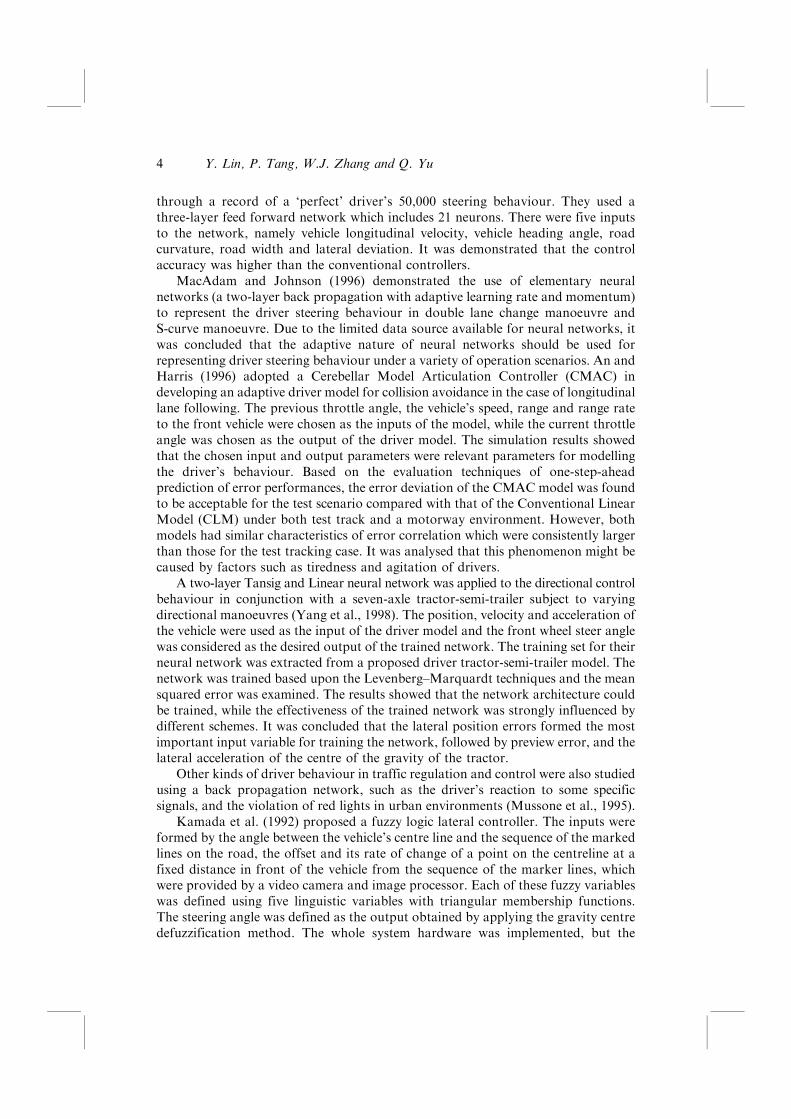
through a record of a `perfect' driver's 50,000 steering behaviour. They used athree-layer feed forward network which includes 21 neurons. There were five inputsto the network, namely vehicle longitudinal velocity, vehicle heading angle, roadcurvature, road width and lateral deviation. It was demonstrated that the controlaccuracy was higher than the conventional controllers.

MacAdam and Johnson (1996) demonstrated the use of elementary neuralnetworks (a two-layer back propagation with adaptive learning rate and momentum)to represent the driver steering behaviour in double lane change manoeuvre andS-curve manoeuvre. Due to the limited data source available for neural networks, itwas concluded that the adaptive nature of neural networks should be used forrepresenting driver steering behaviour under a variety of operation scenarios. An andHarris (1996) adopted a Cerebellar Model Articulation Controller (CMAC) indeveloping an adaptive driver model for collision avoidance in the case of longitudinallane following. The previous throttle angle, the vehicle's speed, range and range rateto the front vehicle were chosen as the inputs of the model, while the current throttleangle was chosen as the output of the driver model. The simulation results showedthat the chosen input and output parameters were relevant parameters for modellingthe driver's behaviour. Based on the evaluation techniques of one-step-aheadprediction of error performances, the error deviation of the CMAC model was foundto be acceptable for the test scenario compared with that of the Conventional LinearModel (CLM) under both test track and a motorway environment. However, bothmodels had similar characteristics of error correlation which were consistently largerthan those for the test tracking case. It was analysed that this phenomenon might becaused by factors such as tiredness and agitation of drivers.

A two-layer Tansig and Linear neural network was applied to the directional controlbehaviour in conjunction with a seven-axle tractor-semi-trailer subject to varyingdirectional manoeuvres (Yang et al., 1998). The position, velocity and acceleration ofthe vehicle were used as the input of the driver model and the front wheel steer anglewas considered as the desired output of the trained network. The training set for theirneural network was extracted from a proposed driver tractor-semi-trailer model. Thenetwork was trained based upon the Levenberg±Marquardt techniques and the meansquared error was examined. The results showed that the network architecture couldbe trained, while the effectiveness of the trained network was strongly influenced bydifferent schemes. It was concluded that the lateral position errors formed the mostimportant input variable for training the network, followed by preview error, and thelateral acceleration of the centre of the gravity of the tractor.

Other kinds of driver behaviour in traffic regulation and control were also studiedusing a back propagation network, such as the driver's reaction to some specificsignals, and the violation of red lights in urban environments (Mussone et al., 1995).

Kamada et al. (1992) proposed a fuzzy logic lateral controller. The inputs wereformed by the angle between the vehicle's centre line and the sequence of the markedlines on the road, the offset and its rate of change of a point on the centreline at afixed distance in front of the vehicle from the sequence of the marker lines, whichwere provided by a video camera and image processor. Each of these fuzzy variableswas defined using five linguistic variables with triangular membership functions.The steering angle was defined as the output obtained by applying the gravity centredefuzzification method. The whole system hardware was implemented, but the

Y. Lin, P. Tang, W.J. Zhang and Q. Yu4

control accuracy was not well validated due to the limited experimental trials.Hessburg and Tomizuka (1993) developed a fuzzy logic controller for vehicle lateralguidance which consisted of three sub-controllers: preview, feedback and gainscheduling. The fuzzy preview controller perceived the curvature for each curvedsection of the reference track and then computed the required steering angle. Thefeedback controller generated the feedback steering angle based on the discrepancybetween the current and the desired state variables. A trade off was made betweenthese two control signals, and the final steering angle was given by the gainscheduling controller. It was reported that a considerable fluctuation existed intheir system.

1.3 Objectives and scope

The literature review shows a general trend in the study of modelling of humanbehaviours, i.e. towards the greater application of computational artificialintelligence approaches, such as the neural network technique and the fuzzy logictheory. Such a trend is sound because the human driver's mental and physicalbehaviour is non-deterministic and highly non-linear, and hence there are seldomany first principles available governing such behaviour; see also the discussionabove. The complexity in predicting human driver behaviours is further coupledwith the complexity in predicting vehicle dynamics (e.g. the friction between the tyreand the road, etc.), as drivers behave under the dynamic situation of the vehicle andthe environment. However, the current literature leaves some room for a furtherstudy. For example, MacAdam and Johnson's work (1996) has some limitations inthat

* they did not consider the velocity and the acceleration of the yaw angle in theirneural network model

* the neural network model they used is elementary

* the way they considered for the driver's preview was through three sensors formeasuring the offsets (the current time t; t� �1, and t� �2, where �1, �2 arespecific delays defined empirically).

The work reported by Yang et al. (1998) considered a tractor and a trailer instead ofa car. Owing to this difference, the inputs to their neural network model might bedifferent from a car. Besides, in their model only lateral motion parameters wereconsidered. The study reported by Atsumi et al. (1993) considered different drivingsituations as the variation of vehicle velocity only. In general, the reported studies inthe literature usually employed relatively simple network architectures to theirparticular problems. It is relatively difficult to generalise about the results in terms ofthe neural network models they used.

The study reported in this paper was a continuing project on the study ofdeveloping a fuzzy logic controller for human driver handling behaviours in a DVEsystem (Gu and Yu, 1993). The primary goal of this study was the development of aneural network-based model for human driver handling behaviour in a DVE system.Consistent with this goal, the following objectives are rendered for this study:

Artificial neural network modelling of driver handling behaviour 5

* Objective 1: to employ and compare more advanced neural networkarchitectures/models in the modelling of driver behaviour.

* Objective 2: to develop a driver±vehicle±environment simulation system, in whichthe driver handling behaviour model is a part of the system.

For Objective 1, different neural network architectures were employed for thesame problem and compared to evaluate their suitability. For Objective 2, a testbed system was developed on which the effectiveness of the developed driverbehaviour model was examined through a comparison of the simulation result(produced from this system) and the experimental result (conducted in this study).The next section presents a general architecture of a driver±vehicle±environmentsimulation system, where a context for a driver handling behaviour model can beexplicitly made.

2 The DVE simulation system

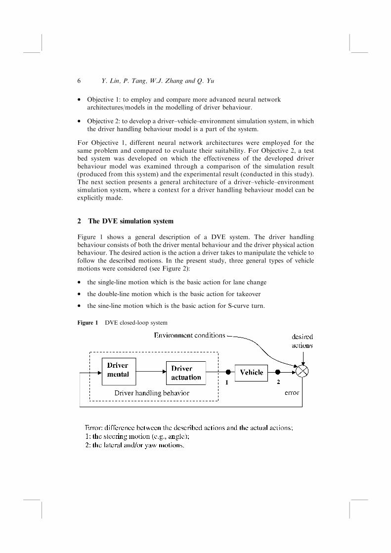
Figure 1 shows a general description of a DVE system. The driver handlingbehaviour consists of both the driver mental behaviour and the driver physical actionbehaviour. The desired action is the action a driver takes to manipulate the vehicle tofollow the described motions. In the present study, three general types of vehiclemotions were considered (see Figure 2):

* the single-line motion which is the basic action for lane change

* the double-line motion which is the basic action for takeover

* the sine-line motion which is the basic action for S-curve turn.

Figure 1 DVE closed-loop system

Y. Lin, P. Tang, W.J. Zhang and Q. Yu6

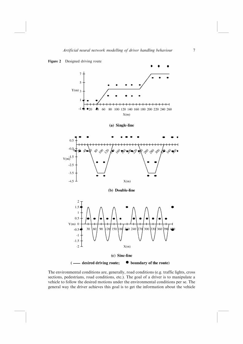
Figure 2 Designed driving route

The environmental conditions are, generally, road conditions (e.g. traffic lights, crosssections, pedestrians, road conditions, etc.). The goal of a driver is to manipulate avehicle to follow the desired motions under the environmental conditions per se. Thegeneral way the driver achieves this goal is to get the information about the vehicle

Artificial neural network modelling of driver handling behaviour 7

dynamics and the error between the desired vehicle motion and the actual vehiclemotion, to make his or her decisions, and to actuate the vehicle (see Figure 1). It isexpected that drivers should have an adaptive control ability for the uncertaintycreated from the environment, the complexity from the vehicle dynamics and fromthe interaction between the driver and the vehicle and between the vehicle and theenvironment.

The computer simulation programme for the DVE system includes threemodules: environment and task input module, vehicle dynamics module and drivercontroller module. At this phase of the study, the environment and task moduleincludes a route library that contains single-line, double-line and sine-line routes andtasks (see Figure 2). The vehicle dynamic model includes a three degree-of-freedom(DOF) vehicle model, owing to a wide agreement that 3 d.o.f. is sufficient torepresent vehicle dynamics when the lateral acceleration is smaller than 0.4 g (Smithand Starkey, 1995). In the present study, we aimed to develop a driver handlingbehaviour model. In this development, the different driving routes and dynamics ofthe vehicle were considered; however the interaction between the environment (e.g.traffic situation) and the driver was not considered.

The DVE system works as follows: The user is required to select a route and givean initial steering angle. Then, the 3-d.o.f. vehicle model calculates the values of thevehicle dynamic variables, namely, lateral acceleration, lateral velocity and yaw anglevelocity. The fourth-order Lounge-Kutta method solves the 3-d.o.f. vehicle model.The lateral displacement is obtained based on the trapezoidal integral method. Thesevariables are used as feedback signals to the driver handling model (see laterdiscussion). The steering wheel angle can be obtained from the driver model, i.e. theneural network model. The updated steering wheel angle is fed to the 3-d.o.f. vehiclemodel, which triggers a new cycle of the process. The next section discusses neuralnetwork models for the DVE system.

3 Neural network model development

3.1 Inputs and outputs to the neural network

To develop a neural network model for the DVE system, the vehicle driving motionsystem is considered as a discrete time-variant system. Let the inputs and outputs tothe neural network model be denoted by INPUT�tk� and OUTPUT�tk� at time tk.The inputs are the information from the vehicle dynamics and the error. Inparticular, the inputs in the present study include:

* the yaw angular velocity r�tk�* the lateral velocity _Y�tk�* the lateral acceleration �Y�tk�* the roll angle '�tk�* the roll angle velocity _'�tk�* the lateral displacement Y�tk�* the preview lateral offset O�tk�.

Y. Lin, P. Tang, W.J. Zhang and Q. Yu8

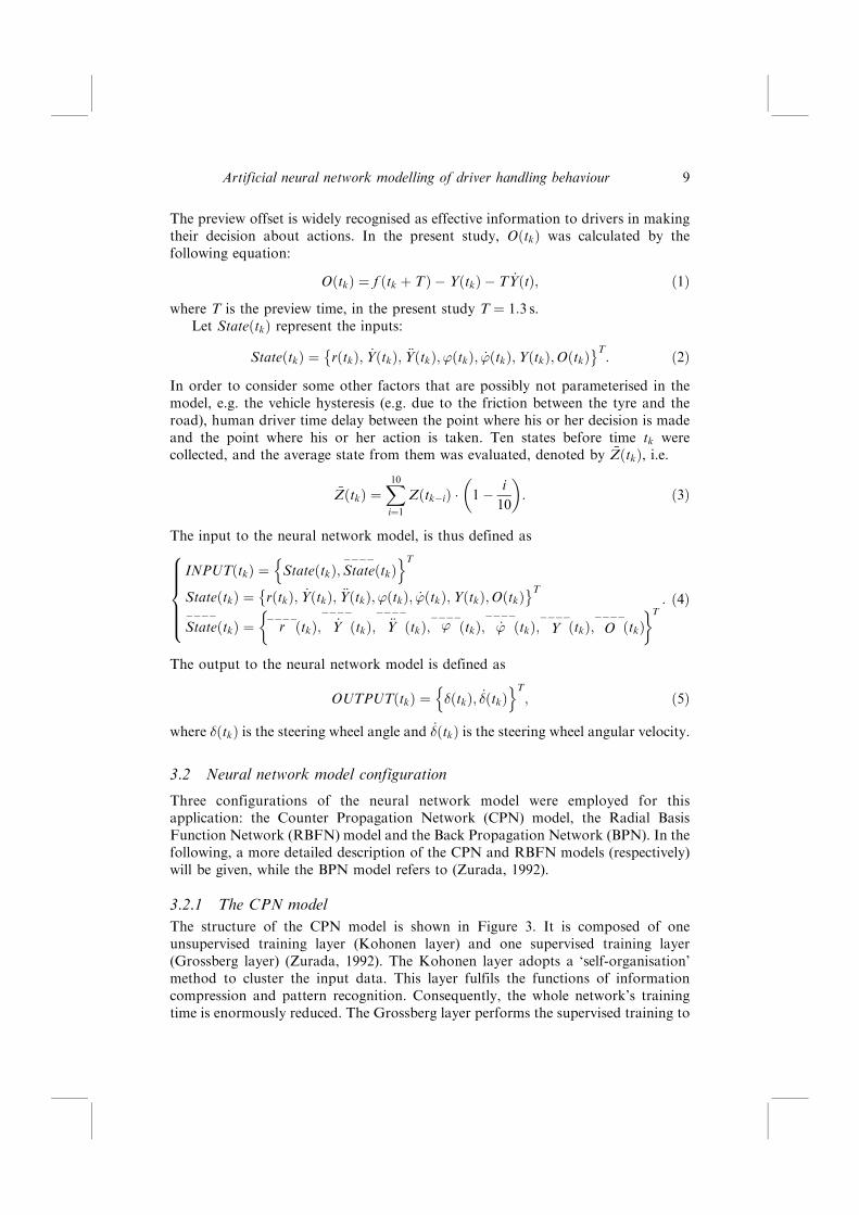
The preview offset is widely recognised as effective information to drivers in makingtheir decision about actions. In the present study, O�tk� was calculated by thefollowing equation:

O tk� � � f tk � T� � ÿ Y tk� � ÿ T _Y t� �; �1�where T is the preview time, in the present study T � 1:3 s.

Let State�tk� represent the inputs:

State tk� � � r tk� �; _Y tk� �; �Y tk� �; ' tk� �; _' tk� �;Y tk� �;O tk� �� T

: �2�In order to consider some other factors that are possibly not parameterised in themodel, e.g. the vehicle hysteresis (e.g. due to the friction between the tyre and theroad), human driver time delay between the point where his or her decision is madeand the point where his or her action is taken. Ten states before time tk werecollected, and the average state from them was evaluated, denoted by �Z�tk�, i.e.

�Z tk� � �X10i�1

Z tkÿi� � � 1ÿ i

10

� �: �3�

The input to the neural network model, is thus defined as

INPUT tk� � � State tk� �;Stateÿÿÿÿ

tk� �n oT

State tk� � � r tk� �; _Y tk� �; �Y tk� �; ' tk� �; _' tk� �;Y tk� �;O tk� �� T

Stateÿÿÿÿ

tk� � � rÿÿÿÿ

tk� �; _Yÿÿÿÿ

tk� �; �Yÿÿÿÿ

tk� �; 'ÿÿÿÿ

tk� �; _'ÿÿÿÿ

tk� �; Yÿÿÿÿ

tk� �; Oÿÿÿÿ

tk� �� �T

8>>>><>>>>: : �4�

The output to the neural network model is defined as

OUTPUT tk� � � � tk� �; _� tk� �n oT

; �5�

where ��tk� is the steering wheel angle and _��tk� is the steering wheel angular velocity.

3.2 Neural network model configuration

Three configurations of the neural network model were employed for thisapplication: the Counter Propagation Network (CPN) model, the Radial BasisFunction Network (RBFN) model and the Back Propagation Network (BPN). In thefollowing, a more detailed description of the CPN and RBFN models (respectively)will be given, while the BPN model refers to (Zurada, 1992).

3.2.1 The CPN model

The structure of the CPN model is shown in Figure 3. It is composed of oneunsupervised training layer (Kohonen layer) and one supervised training layer(Grossberg layer) (Zurada, 1992). The Kohonen layer adopts a `self-organisation'method to cluster the input data. This layer fulfils the functions of informationcompression and pattern recognition. Consequently, the whole network's trainingtime is enormously reduced. The Grossberg layer performs the supervised training to

Artificial neural network modelling of driver handling behaviour 9

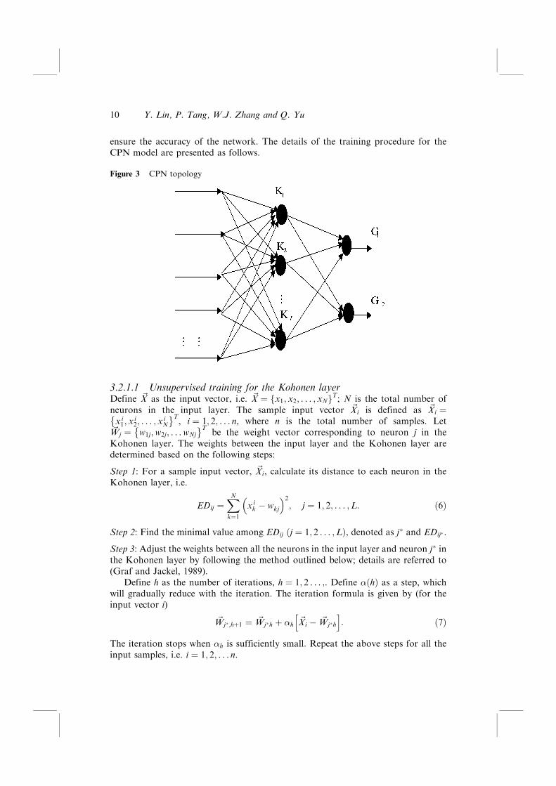
ensure the accuracy of the network. The details of the training procedure for theCPN model are presented as follows.

Figure 3 CPN topology

3.2.1.1 Unsupervised training for the Kohonen layerDefine ~X as the input vector, i.e. ~X � x1; x2; . . . ; xNf gT; N is the total number ofneurons in the input layer. The sample input vector ~Xi is defined as ~Xi �xi1; x

i2; . . . ; xi

N

� T, i � 1; 2; . . . n, where n is the total number of samples. Let

~Wj � w1j;w2j; . . .wNj

� Tbe the weight vector corresponding to neuron j in the

Kohonen layer. The weights between the input layer and the Kohonen layer aredetermined based on the following steps:

Step 1: For a sample input vector, ~Xi, calculate its distance to each neuron in theKohonen layer, i.e.

EDij �XNk�1

xik ÿ wkj

� �2; j � 1; 2; . . . ;L: �6�

Step 2: Find the minimal value among EDij �j � 1; 2 . . . ;L�, denoted as j� and EDij� .

Step 3: Adjust the weights between all the neurons in the input layer and neuron j� inthe Kohonen layer by following the method outlined below; details are referred to(Graf and Jackel, 1989).

Define h as the number of iterations, h � 1; 2 . . . ;. Define ��h� as a step, whichwill gradually reduce with the iteration. The iteration formula is given by (for theinput vector i)

~Wj�;h�1 � ~Wj�h � �h~Xi ÿ ~Wj�h

h i: �7�

The iteration stops when �h is sufficiently small. Repeat the above steps for all theinput samples, i.e. i � 1; 2; . . . n.

Y. Lin, P. Tang, W.J. Zhang and Q. Yu10

3.2.1.2 Supervised training for the Grossberg layerFollowing the training procedure for the Kohonen layer, a set of neurons in theKohonen layer is obtained, which is denoted as Qj� � j�i ji � 1; 2; . . . n

� . The

following procedure applies to the training of the weight between Qj� and the outputlayer. Define ~Bi as the weight vector for the Grossberg layer between a neuronj�i i � 1; 2; . . . n� � and the output layer, i.e.

~Bi � bi1; bi2; . . . biGf g; �8�where G is the total number of neurons in the output layer.

The goal of the training is to determine ~Bi �i � 1; 2; . . . n� by a set of pairs h~Xi; ~Yii,where ~Yi is the output, i.e. ~Yi � yi

1; yi2; . . . y i

G

� T. The basic function for iteration to

determine ~Bi is given by

~Bi;h�1 � ~Bih � � ~Yi ÿ ~Bih

h i; �9�

where � is a constant �0 � � � 1�, given as 0.8 in the present study.The stop criteria for iteration is

~Bh�1 ÿ ~Bh

�� �� � "; �10�where " is a small number.

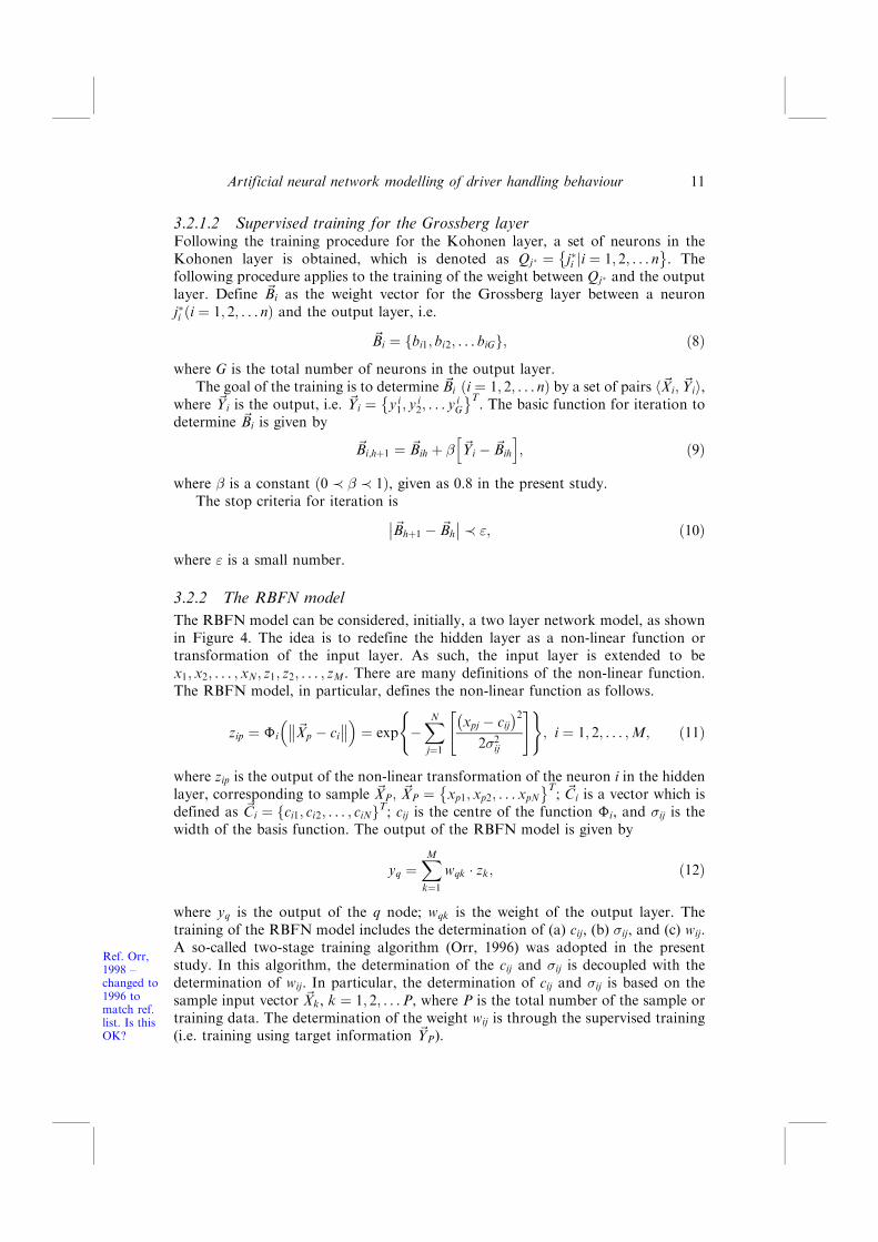
3.2.2 The RBFN model

The RBFN model can be considered, initially, a two layer network model, as shownin Figure 4. The idea is to redefine the hidden layer as a non-linear function ortransformation of the input layer. As such, the input layer is extended to bex1; x2; . . . ; xN; z1; z2; . . . ; zM. There are many definitions of the non-linear function.The RBFN model, in particular, defines the non-linear function as follows.

zip � �i~Xp ÿ ci � �

� exp ÿXNj�1

xpj ÿ cijÿ �2

2�2ij

" #( ); i � 1; 2; . . . ;M; �11�

where zip is the output of the non-linear transformation of the neuron i in the hiddenlayer, corresponding to sample ~XP; ~XP � xp1; xp2; . . . xpN

� T; ~Ci is a vector which is

defined as ~Ci � ci1; ci2; . . . ; ciNf gT; cij is the centre of the function �i, and �ij is thewidth of the basis function. The output of the RBFN model is given by

yq �XMk�1

wqk � zk; �12�

where yq is the output of the q node; wqk is the weight of the output layer. Thetraining of the RBFN model includes the determination of (a) cij, (b) �ij, and (c) wij.A so-called two-stage training algorithm (Orr, 1996) was adopted in the presentstudy. In this algorithm, the determination of the cij and �ij is decoupled with thedetermination of wij. In particular, the determination of cij and �ij is based on thesample input vector ~Xk, k � 1; 2; . . .P, where P is the total number of the sample ortraining data. The determination of the weight wij is through the supervised training(i.e. training using target information ~YP).

Ref. Orr,1998 ±changed to1996 tomatch ref.list. Is thisOK?

Artificial neural network modelling of driver handling behaviour 11

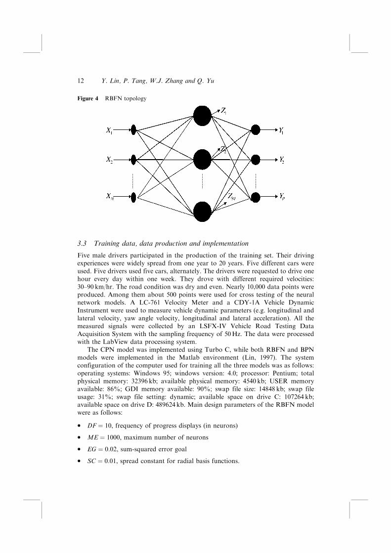
Figure 4 RBFN topology

3.3 Training data, data production and implementation

Five male drivers participated in the production of the training set. Their drivingexperiences were widely spread from one year to 20 years. Five different cars wereused. Five drivers used five cars, alternately. The drivers were requested to drive onehour every day within one week. They drove with different required velocities:30±90 km/hr. The road condition was dry and even. Nearly 10,000 data points wereproduced. Among them about 500 points were used for cross testing of the neuralnetwork models. A LC-761 Velocity Meter and a CDY-1A Vehicle DynamicInstrument were used to measure vehicle dynamic parameters (e.g. longitudinal andlateral velocity, yaw angle velocity, longitudinal and lateral acceleration). All themeasured signals were collected by an LSFX-IV Vehicle Road Testing DataAcquisition System with the sampling frequency of 50Hz. The data were processedwith the LabView data processing system.

The CPN model was implemented using Turbo C, while both RBFN and BPNmodels were implemented in the Matlab environment (Lin, 1997). The systemconfiguration of the computer used for training all the three models was as follows:operating systems: Windows 95; windows version: 4.0; processor: Pentium; totalphysical memory: 32396 kb; available physical memory: 4540 kb; USER memoryavailable: 86%; GDI memory available: 90%; swap file size: 14848 kb; swap fileusage: 31%; swap file setting: dynamic; available space on drive C: 107264 kb;available space on drive D: 489624 kb. Main design parameters of the RBFN modelwere as follows:

* DF � 10, frequency of progress displays (in neurons)

* ME � 1000, maximum number of neurons

* EG � 0:02, sum-squared error goal

* SC � 0:01, spread constant for radial basis functions.

Y. Lin, P. Tang, W.J. Zhang and Q. Yu12

4 Results and discussion

4.1 Comparison between BPN, CPN and RBFN

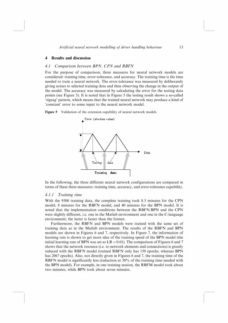
For the purpose of comparison, three measures for neural network models areconsidered: training time, error-tolerance, and accuracy. The training time is the timeneeded to train a neural network. The error-tolerance was measured by deliberatelygiving noises to selected training data and then observing the change in the output ofthe model. The accuracy was measured by calculating the error for the testing datapoints (see Figure 5). It is noted that in Figure 5 the testing result shows a so-called`zigzag' pattern, which means that the trained neural network may produce a kind of`constant' error to some input to the neural network model.

Figure 5 Validation of the extension capability of neural network models

In the following, the three different neural network configurations are compared interms of these three measures: training time, accuracy, and error-tolerance capability.

4.1.1 Training time

With the 9500 training data, the complete training took 8.5 minutes for the CPNmodel, 8 minutes for the RBFN model, and 40 minutes for the BPN model. It isnoted that the implementation conditions between the RBFN/BPN and the CPNwere slightly different, i.e. one in the Matlab environment and one in the C-languageenvironment; the latter is faster than the former.

Furthermore, the RBFN and BPN models were trained with the same set oftraining data as in the Matlab environment. The results of the RBFN and BPNmodels are shown in Figures 6 and 7, respectively. In Figure 7, the information oflearning rate is shown to get more idea of the training speed of the BPN model (theinitial learning rate of BPN was set as LR� 0.01). The comparison of Figures 6 and 7shows that the network resource (i.e. to network elements and connections) is greatlyreduced with the RBFN model (trained RBFN only has 150 epochs; whereas BPNhas 2067 epochs). Also, not directly given in Figures 6 and 7, the training time of theRBFN model is significantly less (reduction at 30% of the training time needed withthe BPN model). For example, in one training session, the RBFM model took abouttwo minutes, while BPN took about seven minutes.

Artificial neural network modelling of driver handling behaviour 13

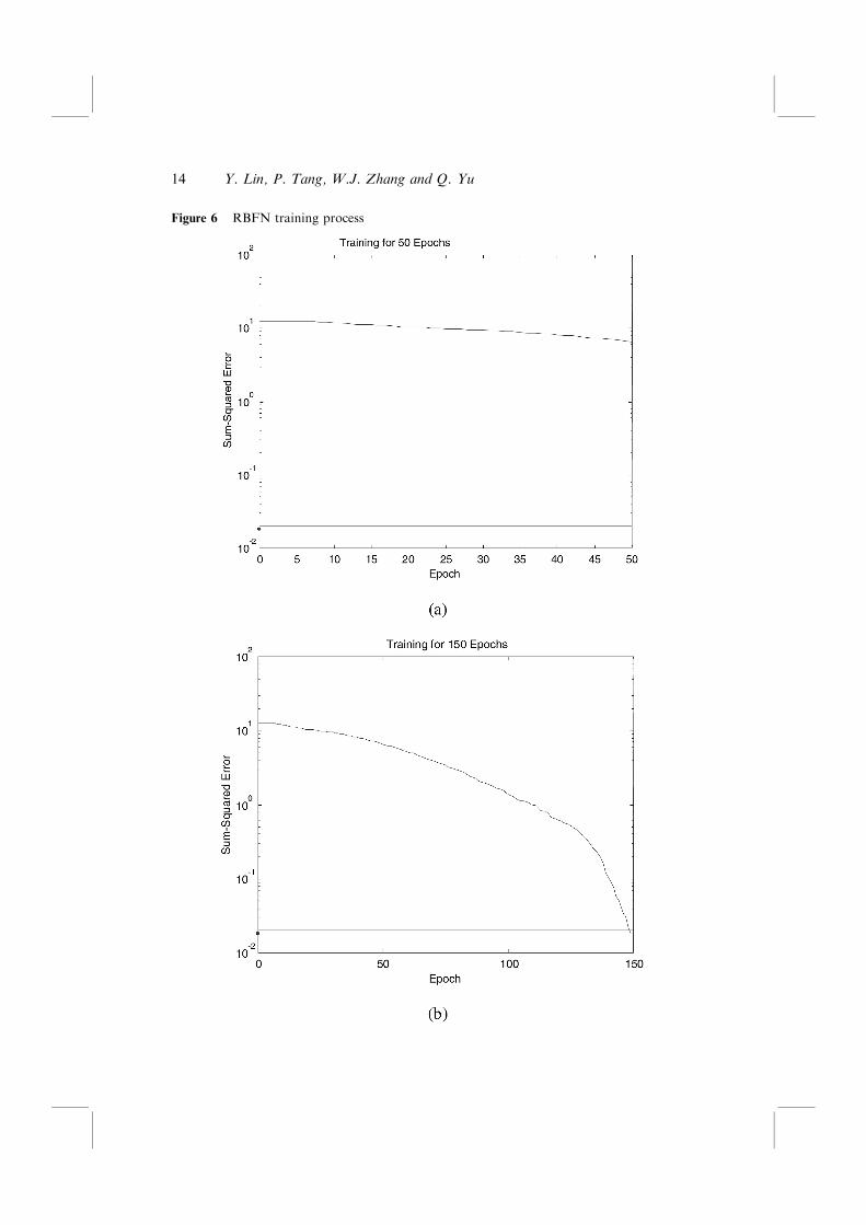
Figure 6 RBFN training process

Y. Lin, P. Tang, W.J. Zhang and Q. Yu14

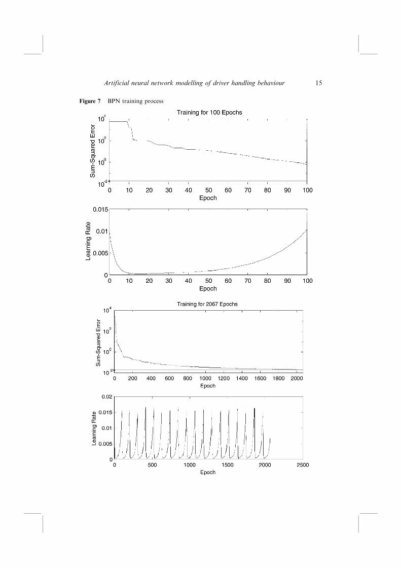
Figure 7 BPN training process

Artificial neural network modelling of driver handling behaviour 15

4.1.2 Error-tolerance capability

It was verified that the CPN model achieved the best error-tolerance resultamongst the three models. This capability with the CPN model is brought about bythe advantages of the weight-updating scheme of the Kohonen layer where theweight-updating scheme was extended to the weights of the vicinity of a node, insteadof a single node. As such, `similar' data tend to be clustered into the same class. TheRBFN model achieved the best accuracy among the three models. In the following,some more detailed results of the RBFN and BPN models were presented.

Furthermore, the error-tolerance was examined through the following idea. TheRBFN model was put into the DVE simulation system (see Figure 1). In the DVEsystem, the vehicle part was a model not a real system. Notice that when the driverbehaviour model was developed, a real vehicle was used to produce the trainingdata and thus further the neural network model. That said, there is a discrepancybetween the training data and the data in the simulation system (produced by thevehicle dynamic model). Such a discrepancy is viewed as a kind of noise of thetraining data.

4.1.3 Accuracy

A cross validation test of the trained RBFN was performed. The result is shown inFigure 8. It can be seen that the maximal error (absolute) is about 0.16 degree. Notethat usually the range of magnitude of the steering angle is about 45 degrees. Therelative maximal error would be 0.4%, which is very small.

In summary, the comparison of BPN, CPN and RBFN is shown in Table 1(H: Highest; M: Medium; L: Lowest):

Table 1 Comparison between BPN, CPN and RBFN

BPN CPN RBFN

Training time H M L

Accuracy M L H

Error-tolerance L H M

4.2 Comparison between simulation results and experimental results

The road experiment was carried out, in which the same device and instruments wereused. The experiment was performed in an open field for the purpose of eliminatingany disturbance, e.g. traffic, etc. (see Figure 9). Two drivers were hired for theexperiment. They were required to drive with different speeds to follow three routes.The drive with these speeds should not make the lateral acceleration of the cargreater than 0.4 g. The payment was concrete and the tyre of the vehicle was full ofair. These experimental conditions ensured the accuracy of the vehicle dynamicsmodel used in the DVE simulation system.

Y. Lin, P. Tang, W.J. Zhang and Q. Yu16

Figure 8 Absolute error of the RBFN model

Artificial neural network modelling of driver handling behaviour 17

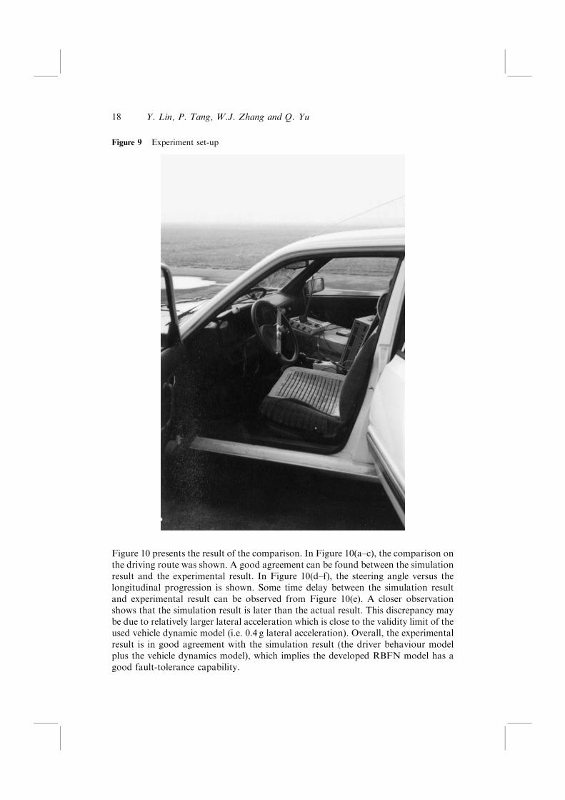
Figure 9 Experiment set-up

Figure 10 presents the result of the comparison. In Figure 10(a±c), the comparison onthe driving route was shown. A good agreement can be found between the simulationresult and the experimental result. In Figure 10(d±f), the steering angle versus thelongitudinal progression is shown. Some time delay between the simulation resultand experimental result can be observed from Figure 10(e). A closer observationshows that the simulation result is later than the actual result. This discrepancy maybe due to relatively larger lateral acceleration which is close to the validity limit of theused vehicle dynamic model (i.e. 0.4 g lateral acceleration). Overall, the experimentalresult is in good agreement with the simulation result (the driver behaviour modelplus the vehicle dynamics model), which implies the developed RBFN model has agood fault-tolerance capability.

Y. Lin, P. Tang, W.J. Zhang and Q. Yu18

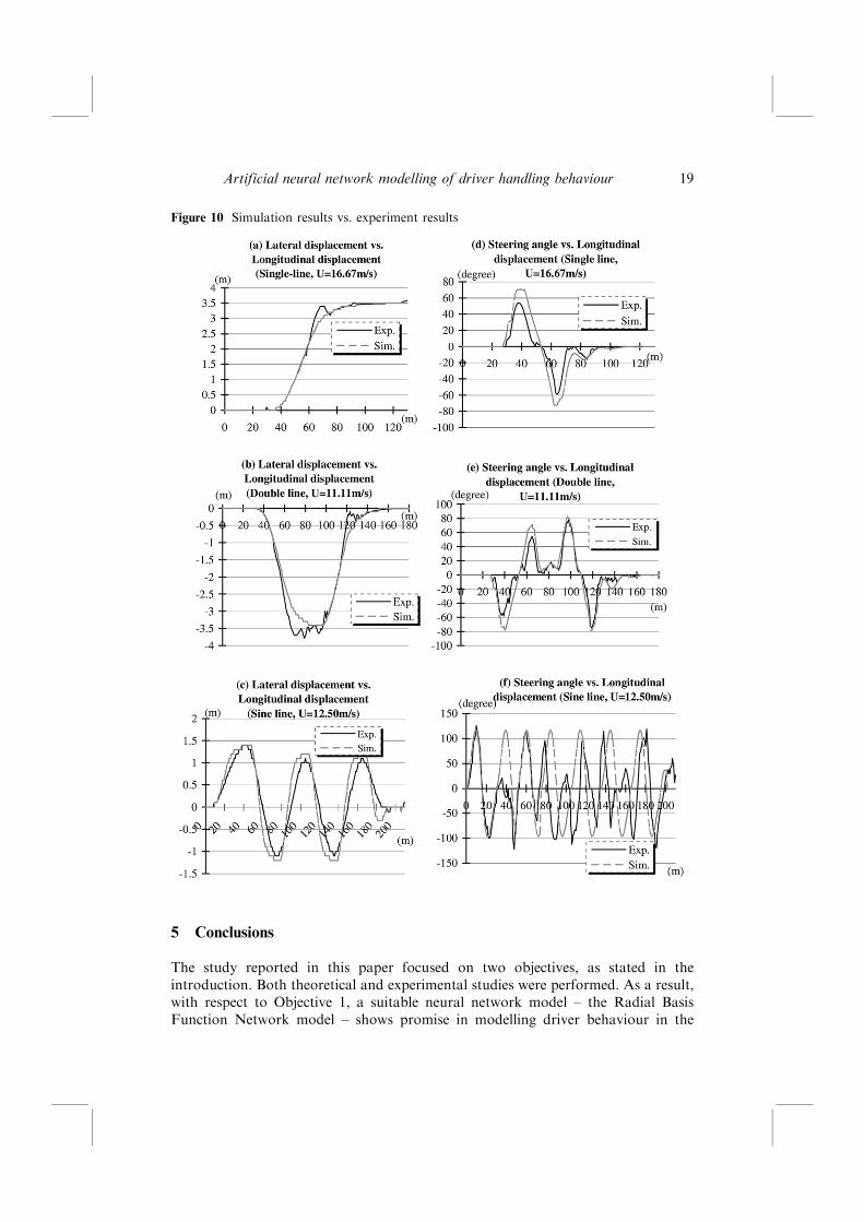
Figure 10 Simulation results vs. experiment results

5 Conclusions

The study reported in this paper focused on two objectives, as stated in theintroduction. Both theoretical and experimental studies were performed. As a result,with respect to Objective 1, a suitable neural network model ± the Radial BasisFunction Network model ± shows promise in modelling driver behaviour in the

Artificial neural network modelling of driver handling behaviour 19

Driver±Vehicle±Environment system. The training time with the Radial BasisFunction Network model can be further reduced by giving constant centre and/or theconstant width of the basis function, or partial constants and partial variants, beingtailored to more specific driving situations. With respect to Objective 2, theDriver±Vehicle±Environment simulation system was developed and the simulationresults were in good agreement with the experimental results.

6 Future work

The discrepancy between the simulation result and the experimental result under thesine route may be alleviated by increasing the preview time. This is where more workneeds to be done. Another possible cause for this delay may be attributed to the effectof driver mental workload, as it was observed that the mental workload of driverwhen driving the sine route is higher than for the single line or double line routes(Lin, 1997). Future work should consider how to incorporate mental workload in thedriver behaviour model. In Lin (1997), the driver's mental workload was alsomeasured, particularly the heart rate and blood pressure. It was found that these twomeasures were sensitive to the situation under interest. One possible way toincorporate the mental workload is to define these two measures as part of the inputto the RBFN model.

Acknowledgement

This work has been supported by the Natural Science and Engineering ResearchCouncil of Canada (NSERC) and Chinese Natural Science Foundation (CNSF). Allthe authors thank these sources of support.

References

Ackermann, J. and Sienel, W. (1990) `Robust control for automatic steering', Proceedings ofthe American Control Conference, pp.795±800.

An, P.E. and Harris, C.J. (1996) `An intelligent driver warning system for vehicle collisionavoidance', IEEE Transactions on Systems, Man and Cybernetics, Part A: Systems andHumans, Vol. 26, No. 2, pp.254±261.

Atsumi, B., Sugiura, S. and Kimura, K. (1993) `Evaluation of mental work load in vehicledriving by analysis of heart rate variability', Proceedings of the Human Factors andErgonomics Society 37th Annual Meeting, pp.574±579.

Colburn, C.J. (1978) `Perceived risk as a determinant of driver behavior', Accident Analysis &Prevention, Vol. 10, pp.131±141.

Ervin, B. and Guy, Y. (1986) `The influence of weights and dimensions on the stability andcontrol of heavy-duty trucks in Canada', University of Michigan Transportation ResearchInstitute (UMTRI) Report, No. 86±35.

Fenton, R.E. (1971) `On the steering of automated vehicles: theory and experiment', IEEETransactions on Automated Control, Vol. AC-21, No. 3, pp.306±315.

Fenton, R.E. (1988) `On the optimal design of an automotive lateral controller', IEEETransactions on Vehicular Technology, Vol. 37, No. 2, pp.108±113.

Y. Lin, P. Tang, W.J. Zhang and Q. Yu20

Graf, H.P. and Jackel, L.D. (1989) `An electronic neural network circuits', IEEE Circuits andDevices Magazine (July), pp.44±48.

Gu, X. and Yu, Q. (1993) `Driver-vehicle-environment closed-loop simulation of handling andstability using fuzzy control theory', Proceedings of 13th IAVSD Symposium, Chengdu,China, pp.172±181.

Hessburg, T. and Tomizuka, M. (1993) `Fuzzy logic control for lateral vehicle guidance',Proceedings of the IEEE Conference on Control Applications, Vol. 2, pp.581±586.

Kamada, H., Gotoh, T. and Yoshida, M. (1992) `Visual control system using image processingand fuzzy inferences', Systems and Computers in Japan, Vol. 23, No. 3, pp.13±25.

Kiencke, U., Majjad, R. and Kramer, S. (1999) `Modeling and performance analysis of ahybrid driver model', Control Engineering Practice, Vol. 7, No. 8, pp.985±991.

Kornhauser, A.L. (1991) `Neural network approaches for lateral control of autonomoushighway vehicles', VNIS '91 Vehicle Navigation and Information Systems Conference, Vol.2, pp.1143±1145.

LeBlanc, D. and Ervin, R.J. (1996) `CPAC: an implementation of a road-departure warningsystem', IEEE Contr. Syst. Mag., Vol. 16, pp.61±71.

Lee, A.Y. (1989) `Algorithm for four-wheel-steering passenger vehicles', Advanced AutomotiveTechnologies, pp.83±98.

Lin, Y. (1997) Study on Handling Stability of Driver±Vehicle±Environment Closed-loop SystemBased on Neural Networks and Fuzzy Theory, PhD thesis, China Agricultural University.

Lin, Y. and Yu, Q. (1996) `A study on driver model using neural network systems', TheProceedings of the 12th ISTVS International Conference, Beijing, China, Oct. 7±11,pp.341±348.

MacAdam, C.C. (1980) `An optimal preview control for linear systems', Journal of DynamicSystems, Measurement and Control, Transactions of the ASME, Vol. 102, No. 3,pp.188±190.

MacAdam, C.C. (1981) `Application of an optimal preview control for simulation of closed-loopautomobile driving', IEEE Transactions on System, Man and Cybernetics, SMC-11, Vol. 6.

MacAdam, C.C. and Johnson, G.E. (1996) `Application of elementary neural networks andpreview sensors for representing driver steering control behavior', Vehicle SystemDynamics, Vol. 25, pp.3±30.

Mussone, L., Reitani, G. and Rinelli, S. (1995) `An ANN model to study driver behavior inurban environment', 10th International Conference on the Applications of ArtificialIntelligence in Engineering, pp.419±426.

Neusser, S. (1993) `Neural control for lateral vehicle guidance', IEEE Micro, pp.57±66.

Orr, M.J.L. (1996) `Introduction to redial basis function networks', Technical Report (April),Centre for Cognitive Science, University of Edinburgh.

Peng, H. (1994) `A reusability study of vehicle lateral control system', Vehicle SystemDynamics, Vol. 23.

Peng, H. and Tomizuka, M. (1991) `Preview control for vehicle lateral guidance in highwayautomation', Proceedings of the 1991 American Control Conference, pp.2621±2627 (alsoASME Journal of Dynamic Systems, Measurements and Control, 1993, Vol. 115,pp.679±686).

Pham, H.A., Hedrick, J.K. and Tomizuka, M. (1994) `Combined lateral and longitudinalcontrol of vehicles for automated highway systems', Proceedings of the 1994 AmericanControl Conference, Baltimore, MD.

Shepanski, J.F. and Macy, S.A. (1987) `Manual training techniques of autonomous systemsbased on artificial neural networks', IEEE 1st International Conference on NeuralNetworks, pp.21±24.

MacAdam,1981 ±pleasesupply no.of journaland pagerange.

Artificial neural network modelling of driver handling behaviour 21

Shladover, S.E. and Desoer, C.A. (1991) `Automatic vehicle control developments in thePATH program', IEEE Transactions on Vehicular Technology, Vol. 40, pp.114±130.

Smith, D.E. and Starkey, J.M. (1995) `Effects of model complexity on the performance ofautomated vehicle steering controllers: model development, validation and comparison',Vehicle System Dynamics, Vol. 24, pp.163±181.

Tang, P. and Mann, D.D. (2003) `Ergonomic requirements of a visual information display unitused for guidance of agricultural vehicles', Journal of Agricultural Safety and Health, Vol.9, No. 1, pp.47±60.

Wilde, G.J.S. (1988) `Risk homeostasis theory and traffic accidents ± propositions, deductionsand discussion of dissension in recent reactions', Ergonomics, Vol. 31, No. 4, pp.441±468.

Yang, X., Stiharu, I. and Rakheja, S. (1998) `Study of driver factors affecting the directionalresponse of an articulated vehicle using neural networks', Transactions of CSME, Vol. 22,No. 3, pp.291±306.

Zhang, W.J. (2003) `A remark on modeling of complex systems', Technical Report(AEDL-WJZ-2003-02), Advanced Engineering Design Laboratory, University ofSaskatchewan.

Zurada, J.M. (1992) Introduction to Artificial Neural Systems, St. Paul, MN: West PublishingCompany.

Y. Lin, P. Tang, W.J. Zhang and Q. Yu22