Improving off-road vehicle handling using an active anti-roll bar
110
Improving off‐road vehicle handling using an active anti‐roll bar by Paul Hendrik Cronjé Submitted in partial fulfilment of the requirements for the degree Masters in Engineering (Mechanical Engineering) in the Faculty of Engineering, Built Environment and Information Technology (EBIT) University of Pretoria Pretoria October 2008 © University of Pretoria
-
Upload
khangminh22 -
Category
Documents
-
view
0 -
download
0
Transcript of Improving off-road vehicle handling using an active anti-roll bar

Improving off‐road vehicle handling
using an active anti‐roll bar
by
Paul Hendrik Cronjé
Submitted in partial fulfilment of the requirements for the degree
Masters in Engineering
(Mechanical Engineering)
in the
Faculty of Engineering, Built Environment
and Information Technology (EBIT)
University of Pretoria
Pretoria
October 2008
©© UUnniivveerrssiittyy ooff PPrreettoorriiaa
Page | ii
Summary
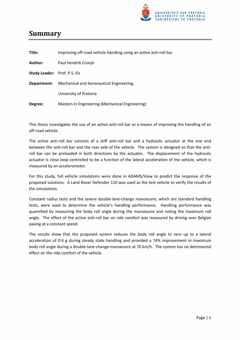
Title: Improving off‐road vehicle handling using an active anti‐roll bar
Author: Paul Hendrik Cronjé
Study Leader: Prof. P.S. Els
Department: Mechanical and Aeronautical Engineering,
University of Pretoria
Degree: Masters in Engineering (Mechanical Engineering)
This thesis investigates the use of an active anti‐roll bar as a means of improving the handling of an off‐road vehicle.
The active anti‐roll bar consists of a stiff anti‐roll bar and a hydraulic actuator at the one end between the anti‐roll bar and the rear axle of the vehicle. The system is designed so that the anti‐roll bar can be preloaded in both directions by the actuator. The displacement of the hydraulic actuator is close loop controlled to be a function of the lateral acceleration of the vehicle, which is measured by an accelerometer.
For this study, full vehicle simulations were done in ADAMS/View to predict the response of the proposed solutions. A Land Rover Defender 110 was used as the test vehicle to verify the results of the simulations.
Constant radius tests and the severe double‐lane‐change manoeuvre, which are standard handling tests, were used to determine the vehicle’s handling performance. Handling performance was quantified by measuring the body roll angle during the manoeuvre and noting the maximum roll angle. The effect of the active anti‐roll bar on ride comfort was measured by driving over Belgian paving at a constant speed.
The results show that the proposed system reduces the body roll angle to zero up to a lateral acceleration of 0.4 g during steady state handling and provided a 74% improvement in maximum body roll angle during a double‐lane‐change‐manoeuvre at 70 km/h. The system has no detrimental effect on the ride comfort of the vehicle.

Page | iii
Opsomming
Titel: Verbetering van die hantering van ‘n veldvoertuig deur die gebruik van ‘n aktiewe teenrolstaaf
Outeur: Paul Hendrik Cronjé
Studieleier: Prof. P.S. Els
Departement: Meganiese en Lugvaartkundige Ingenieurswese,
Universiteit van Pretoria
Degree: Magister in Ingenieurswese (Meganiese Ingenieurswese)
Hierdie tesis ondersoek die gebruik van ‘n aktiewe teenrolstaaf om die hantering van ‘n veldvoertuig te verbeter.
Hierdie aktiewe teenrolstaaf bestaan uit ‘n stywe teenrolstaaf en ‘n hidrouliese aktueerder aan die een kant tussen die teenrolstaaf en die agterste as van die voertuig. Die sisteem is so ontwerp dat die aktueerder in beide rigtings kan beheer. Die hidrouliese aktueerder word deur ‘n geslote lus beheerstelsel beheer, as ‘n funksie van die laterale versnelling op die voertuig wat met ‘n versnellingsmeter gemeet word.
Vir die doel van hierdie studie is vol voertuig model simulasies in ADAMS/View gedoen om die gedrag van die voertuig met die aktiewe teenrolstaaf te voorspel. ‘n Land Rover Defender 110 veldvoertuig is gebruik om die sisteem te toets en resultate wat deur die simulasies verkry is, te verifieer.
Die konstante‐radius‐toets en die dubbelbaanveranderingsmaneuver, wat standaard hanteringstoetse is, is gebruik om die voertuig se hanteringprestasie te meet. Hantering is gekwantifiseer deur die bakrolhoek gedurende die maneuver te meet en die maksimum rolhoek te noteer. Die sisteem se invloed op die ritgemak van die voertuig is ook bepaal deur teen ‘n konstante spoed oor Belgiese plaveisel te ry.
Die resultate wys dat die voorgestelde oplossing die bakrolhoek uitkanselleer tot op ‘n laterale versnelling van 0.4 g tydens ‘n gestadigde hanteringstoets en ‘n verbetering van 74% gee in die maksimum bakrolhoek, gemeet tydens die dubbel‐baan‐veranderings‐maneuver teen ‘n spoed van 70 km/h. Verdere toetse wys dat dié sisteem geen negatiewe uitwerking op die ritgemak van die voertuig het nie.
Page | iv
Acknowledgments
• Our heavenly Father who gave me the power to complete this project to the best of my abilities.
• Prof. Schalk Els, my study leader, for his endless contributions and guidance.
• My parents and Ritali (my fiancée) for their support and encouragement.
• Michael Thoresson for his excellent assistance with ADAMS.
• Juanita van der Walt for her help with the hydraulics.
• All my family and friends for their motivation, help and encouragement.

Page | v
Table of contents
Summary ................................................................................................................................................. ii
Opsomming ............................................................................................................................................ iii
Acknowledgments .................................................................................................................................. iv
Table of contents .................................................................................................................................... v
List of symbols ...................................................................................................................................... viii
List of abbreviations ............................................................................................................................... xi
List of figures ......................................................................................................................................... xii
List of tables .......................................................................................................................................... xv
1 Introduction .................................................................................................................................... 2
2 Literature study ............................................................................................................................... 3
2.1 Statistics about handling accidents ......................................................................................... 3
2.2 Handling .................................................................................................................................. 4
2.3 Ride comfort ........................................................................................................................... 6
2.4 Low‐speed turning .................................................................................................................. 7
2.5 High speed cornering .............................................................................................................. 8
2.5.1 Tyre forces and the magic formula ................................................................................. 8
2.5.2 Cornering equations ...................................................................................................... 11
2.5.3 Understeer gradient ...................................................................................................... 14
2.5.4 Roll moment distribution .............................................................................................. 15
2.6 Proposed solutions ................................................................................................................ 20
2.6.1 Passive suspension ........................................................................................................ 20
2.6.2 Four state semi‐active suspension system (4S4) ........................................................... 21
2.6.3 Other semi‐active suspension systems ......................................................................... 25
2.6.4 Active anti‐roll bars ....................................................................................................... 26
2.6.5 Active suspension .......................................................................................................... 28
2.6.6 Tilting vehicles ............................................................................................................... 29
2.6.7 Selection of proposed solutions .................................................................................... 30
2.7 Conclusion ............................................................................................................................. 32
3 Simulations .................................................................................................................................... 33
3.1 Simulation model .................................................................................................................. 33
3.2 Road type and manoeuvres .................................................................................................. 39

Page | vi
3.3 Validation of simulation model ............................................................................................. 42
3.3.1 Spring and damper characteristics ............................................................................... 42
3.3.2 Tyre characteristics ....................................................................................................... 43
3.3.3 CG height ....................................................................................................................... 46
3.3.4 Chassis torsional stiffness ............................................................................................. 46
3.3.5 Baseline correlation ...................................................................................................... 47
3.4 Simulate proposed solution .................................................................................................. 48
3.5 Conclusion ............................................................................................................................. 53
4 Active anti‐roll bar design, development and testing ................................................................... 54
4.1 Design and manufacturing .................................................................................................... 54
4.2 Bench testing ........................................................................................................................ 58
4.3 Vehicle implementation ........................................................................................................ 61
4.4 Conclusion ............................................................................................................................. 65
5 Results ........................................................................................................................................... 66
5.1 Constant radius test .............................................................................................................. 66
5.2 Double‐lane‐change‐test ...................................................................................................... 67
5.3 Belgian paving test ................................................................................................................ 67
5.4 Test session 1 ........................................................................................................................ 69
5.4.1 Constant radius test ...................................................................................................... 69
5.4.2 Double‐lane‐change‐test .............................................................................................. 70
5.4.3 Belgian paving test ........................................................................................................ 71
5.4.4 Adjustments after test session 1 ................................................................................... 72
5.5 Test session 2 ........................................................................................................................ 74
5.5.1 Constant radius test ...................................................................................................... 74
5.5.2 Double‐lane‐change‐test .............................................................................................. 76
5.5.3 Belgian paving test ........................................................................................................ 78
5.5.4 Adjustments after test session 2 ................................................................................... 79
5.6 Test session 3 ........................................................................................................................ 80
5.6.1 Constant radius test ...................................................................................................... 80
5.6.2 Double‐lane‐change‐test .............................................................................................. 81
5.7 Simulation adjustments ........................................................................................................ 83
5.8 Conclusion ............................................................................................................................. 90
6 Conclusion ..................................................................................................................................... 92
7 Future work ................................................................................................................................... 93

Page | vii
8 Bibliography .................................................................................................................................. 94

Page | viii
List of symbols
A
Area (m2)
a
Acceleration (m/s2)
ya
Lateral acceleration (g)
1a Load dependency on lateral friction (magic formula)
2a Lateral friction level (magic formula)
3a Maximum cornering stiffness (at 0γ = , magic formula)
4a Load at maximum cornering stiffness (magic formula)
5a Chamber sensitivity of cornering stiffness (magic formula)
6 13a a→ Other magic formula coefficients
B Stiffness factor (magic formula)
b Distance between the front axle and the centre of gravity point (m)
C Shape factor (magic formula)
Cα Cornering stiffness (N/°)
fCα Cornering stiffness of the front tyres (N/°)
rCα Cornering stiffness of the rear tyres (N/°)
c Distance between the rear axle and the centre of gravity point (m)
D Peak factor (magic formula)
d Diameter (m)
E Curvature factor (magic formula)
F
Force (N)
yF
Lateral force (N)
yfF
Lateral force on the front axle (N)

Page | ix
yrF
Lateral force on the rear axle (N)
zF
Vertical force (N)
yif
Lateral force on the inside wheel (N)
yof
Lateral force on the outside wheel (N)
zif
Vertical force on the inside wheel (N)
zof
Vertical force on the outside wheel (N)
G Shear modulus of elasticity (Pa)
g Gravitational acceleration = 9.81 (m/s2)
CGh Height of centre of gravity point (m)
rh Height of roll centre (m)
pI Polar moment of inertia (m4)
K Understeer gradient (°/g)
tk Torsional stiffness (Nm/°)
L Length (m), wheelbase (m)
M
Mass of the vehicle (kg)
cgM Moment about the centre of gravity (Nm)
OM
Moments about the contact patch of the outside wheel (Nm)
m
Mass (kg)
n Amount of moles of gas (mol )
P Pressure (Pa )
R
Radius of the turn (m), universal gas constant 1 18.314 . .J mol K− −=
r
Radius (m)
hS Offset on the horizontal axis (magic formula)

Page | x
vS Offset on the vertical axis (magic formula)
T Temperature ( K ), torque (Nm)
t Track width (m)
V
Forward velocity (m/s), volume ( 3m )
bW British Standard 6841 vertical acceleration filter
fW
Load on the front axle (kg)
rW Load on the rear axle (kg)
X Slip angle (°, magic formula)
x Slip angle without vertical adjustment (°, magic formula)
Y Lateral force (N, magic formula)
y Lateral force without vertical adjustment (N, magic formula)
Greek symbols:
α Slip angle (°)
fα Front slip angle (°)
rα Rear slip angle (°)
γ Camber angle (°)
φ
Body roll angle (°)
δ Average steering angle of the front wheels (°)
iδ Steering angle of the inside wheel (°)
oδ Steering angle of the outside wheel (°)
maxτ
Maximum shear stress (Pa)
μ Friction coefficient between the tyres and the road
sμ Static friction coefficient
ymμ
Lateral friction coefficient
Page | xi
List of abbreviations
AARB Active anti‐roll bar
ADAMS Automatic dynamic analysis of mechanical systems
ARB Anti‐roll bar
ASTM American society for testing and materials
DC Direct current
CAD Computer aided design
CDC Continuous damping control
CG Centre of gravity
Deg Degree (°)
DLC Double‐lane‐change
ESC Electronic stability control
ESP Electronic stability program
ISO International Organisation for Standardisation
LF Left front
LR Left rear
NHTSA National highway traffic safety administration
NTV Narrow tilting vehicle
RF Right front
RMS Root mean square
RR Right rear
RRMS Running root mean square
SIA Steering input augmented
SSF Safety stability factor
STC Steering tilt control
SUV Sports utility vehicle
UCC Unified chassis control
PID Proportional integral derivative
Page | xii
List of figures
Figure 2.1: The number of rollover fatalities per million registered vehicles for different types of vehicles in the United States, averaged from 1985 to 1990 (Dukkipati et al., 2008). ........................... 3 Figure 2.2: Passenger vehicles involved in fatal accidents, by vehicle body type and year in the United States (Dukkipati et al., 2008). ............................................................................................................... 4 Figure 2.3: Lane change track and designation of track (International Organisation for Standardisation, 1975). .......................................................................................................................... 5 Figure 2.4: Placing of cones for marking the lane‐change track (International Organisation for Standardisation, 1975). .......................................................................................................................... 5 Figure 2.5: Weighting function Wb used for measuring vibration on a seated person in the vertical direction. ................................................................................................................................................. 6 Figure 2.6: Geometry of a turning vehicle at low speed (Gillespie, 1992). ............................................ 7 Figure 2.7: Tyre cornering force properties (Gillespie, 1992). ............................................................... 8 Figure 2.8: Typical shape of the Magic Formula representing the lateral tyre stiffness (Bakker et al., 1989). .................................................................................................................................................... 10 Figure 2.9: Bicycle model during high speed cornering (Gillespie, 1992). ........................................... 12 Figure 2.10: Change of steering angle with speed for vehicles with different steering characteristics (Gillespie, 1992). ................................................................................................................................... 15 Figure 2.11: Force analysis of a vehicle during cornering (Gillespie, 1992). ........................................ 16 Figure 2.12: Vertical force vs. vertical load characteristic of the tyre (Gillespie, 1992). ..................... 17 Figure 2.13: Kinetic system during body roll (Wilde et al., 2005). ....................................................... 20 Figure 2.14: Kinetic system during vehicle articulation (Wilde et al., 2005). ....................................... 21 Figure 2.15: Circuit diagram of the 4S4 (Els, 2006). .............................................................................. 22 Figure 2.16: Schematic representation of the 4S4 (Els, 2006). ............................................................. 23 Figure 2.17: Soft and stiff spring characteristics of the 4S4 (Els, 2006). ............................................... 24 Figure 2.18: Soft and stiff damping characteristics of the 4S4 (Els, 2006). ........................................... 24 Figure 2.19: Schematics of proposed solution by Packer (1978). ........................................................ 28 Figure 2.20: Narrow tilting vehicle (Gohl et al. 2004). ......................................................................... 30 Figure 3.1: Simulation interaction. ....................................................................................................... 33 Figure 3.2: ADAMS/View model used for the simulations. .................................................................. 34 Figure 3.3: Tyre side force vs. slip angle characteristics (Els, 2006). .................................................... 35 Figure 3.4: Front suspension modelled in ADAMS (Els, 2006). ............................................................. 35 Figure 3.5: Schematic of front suspension model. ............................................................................... 36 Figure 3.6: Rear suspension modelled in ADAMS (Els, 2006). .............................................................. 37 Figure 3.7: Schematic of rear suspension model. ................................................................................. 38 Figure 3.8: Belgian paving on suspension track at Gerotek (Gerotek Test Facilities, 2008). ............... 39 Figure 3.9: Belgian paving used in simulations to perform a DLC manoeuvre. .................................... 40 Figure 3.10: Fingers measuring the surface profile of the Belgian paving (Becker, 2008). ................. 40 Figure 3.11: Electronic format of the Belgian paving (Becker, 2008). .................................................. 41 Figure 3.12: Percentage difference between the measured and simulated weighted RMS values (Becker, 2008). ...................................................................................................................................... 41 Figure 3.13: Soft and stiff spring calculations (Els, 2006). .................................................................... 42

Page | xiii
Figure 3.14: 4S4 damper characteristics (Els, 2007). ............................................................................. 43 Figure 3.15: Lateral force vs. slip angle for the three Pacejka ’89 tyre models at a vertical load of 10 kN. ......................................................................................................................................................... 44 Figure 3.16: Tyres suitable for different simulations conditions (MSC ADAMS, 2007). ...................... 45 Figure 3.17: Results of the same simulations with the three tyre models. .......................................... 46 Figure 3.18: Results of baseline vehicle and simulation during DLC manoeuvre with soft suspension. .............................................................................................................................................................. 47 Figure 3.19: Results of baseline vehicle and simulation during DLC manoeuvre with stiff suspension. .............................................................................................................................................................. 48 Figure 3.20: Anti‐roll bar modelled in ADAMS. ..................................................................................... 49 Figure 3.21: Right hand side of ARB as modelled in ADAMS. ............................................................... 49 Figure 3.22: Left hand side of ARB as modelled in ADAMS. ................................................................. 50 Figure 3.23: Schematic of ARB model. .................................................................................................. 50 Figure 3.24: Average body roll angle of the test vehicle during a DLC manoeuvre at 70km/h on a concrete road. ....................................................................................................................................... 51 Figure 3.25: Average body roll angle of the test vehicle during a DLC manoeuvre at 50km/h on Belgian paving. ...................................................................................................................................... 52 Figure 4.1: CAD of AARB system. .......................................................................................................... 54 Figure 4.2: CAD view of the hydraulic cylinder design. ......................................................................... 56 Figure 4.3: The manufactured hydraulic cylinder. ................................................................................ 57 Figure 4.4: MOOG hydraulic servo valve used to control the hydraulic cylinder and the bypass valve. .............................................................................................................................................................. 57 Figure 4.5: Stone hydraulic power pack. ............................................................................................... 58 Figure 4.6: The manufactured ARB. ...................................................................................................... 59 Figure 4.7: ARB test bench setup. ......................................................................................................... 59 Figure 4.8: Measured torsional stiffness of ARB. .................................................................................. 60 Figure 4.9: Strain gauge to measure torsion in the ARB. ...................................................................... 61 Figure 4.10: AARB fitted to the test vehicle. ........................................................................................ 62 Figure 4.11: AARB fastened on the left hand side to the rear axle. ..................................................... 63 Figure 4.12: ARB fastened on the right hand side to the rear axle. ..................................................... 63 Figure 4.13: PC 104 form factor computer. .......................................................................................... 64 Figure 5.1: Test vehicle during a constant radius test. ......................................................................... 66 Figure 5.2: DLC manoeuvre sequence. ................................................................................................. 68 Figure 5.3: Belgian paving test run. ...................................................................................................... 68 Figure 5.4: Constant radius test: average body roll angle vs. lateral acceleration. .............................. 69 Figure 5.5: DLC test: average body roll angle vs. time. ......................................................................... 70 Figure 5.6: DLC test: lateral acceleration, ARB torque and average body roll angle vs. time. ............. 71 Figure 5.7: Belgian paving test: FFT of vertical acceleration. ............................................................... 72 Figure 5.8: Response of cylinder with and without the Bessel filter. ................................................... 73 Figure 5.9: Effect of different filters on lateral acceleration. ............................................................... 74 Figure 5.10: Constant radius test: average body roll angle vs. lateral acceleration with soft suspension. ........................................................................................................................................... 75 Figure 5.11: Constant radius test: average body roll angle vs. lateral acceleration with stiff suspension. ........................................................................................................................................... 75 Figure 5.12: DLC test: average body roll angle vs. time with soft suspension. ..................................... 76

Page | xiv
Figure 5.13: DLC test: average body roll angle vs. time with stiff suspension. ..................................... 77 Figure 5.14: DLC test: lateral acceleration, ARB torque and average body roll angle vs. time. ........... 77 Figure 5.15: Belgian paving test: FFT of vertical acceleration. ............................................................. 78 Figure 5.16: Steering angles during three DLC manoeuvres with soft suspension. ............................. 79 Figure 5.17: Constant radius test: average body roll angle vs. lateral acceleration with soft suspension. ........................................................................................................................................... 80 Figure 5.18: Constant radius test: average body roll angle vs. lateral acceleration with stiff suspension. ........................................................................................................................................... 81 Figure 5.19: DLC test: average body roll angle vs. time with soft suspension. ..................................... 82 Figure 5.20: DLC test: average body roll angle vs. time with stiff suspension. ..................................... 82 Figure 5.21: Initial and modified torsional stiffness. ............................................................................ 83 Figure 5.22: ARB torsion damper spline. .............................................................................................. 84 Figure 5.23: Correlation between the measured and simulated DLC data with measured actuator displacement. ........................................................................................................................................ 85 Figure 5.24: Lateral force vs. slip angle of the left rear tyre during a DLC manoeuvre at 70 km/h. .... 85 Figure 5.25: Correlation between the measured and simulated DLC data with computed actuator displacement. ........................................................................................................................................ 86 Figure 5.26: ARB torque vs. time of the measured and simulated results during the DLC manoeuvre. .............................................................................................................................................................. 86 Figure 5.27: Effect of friction on the model during a constant radius test. ......................................... 87 Figure 5.28: Effect of friction on the model during a DLC manoeuvre. ................................................ 88 Figure 5.29: Graph of how the modified friction is modelled. ............................................................. 89 Figure 5.30: Effect of modified friction on the model during a constant radius test. .......................... 89 Figure 5.31: Effect of modified friction on the model during a DLC manoeuvre. ................................ 90

Page | xv
List of tables
Table 1: Lane change track dimensions (International Organisation for Standardisation, 1975). ....... 5 Table 2: Guidelines for comfort according to weighted RMS (British Standards Institution, 1987). .... 6 Table 3: Proposed solution weighting table. ........................................................................................ 31 Table 4: Lateral stiffness coefficients used for the Pacejka ’89 tyre model. ........................................ 44 Table 5: Design parameters obtained from simulations: ..................................................................... 52 Table 6: Sensors on test vehicle used during tests. .............................................................................. 64 Table 7: Constant radius test runs done. .............................................................................................. 67 Table 8: Belgian paving test runs done. ................................................................................................ 67 Table 9: Results of weighted RMS on vertical acceleration of Belgian paving test runs. ..................... 71 Table 10: Weighted RMS on vertical acceleration with different filters. ............................................. 73 Table 11: Results of weighted RMS on vertical acceleration for Belgian paving test runs. .................. 78

Page | 2
1 Introduction
The purpose of a vehicle suspension system can be summarised as follows:
• To isolate the vehicle from the uncomfortable vibrations transmitted from the road through the tyres; and
• To transmit the control forces back to the tyres so that the driver can keep the vehicle under control.
To design a vehicle’s suspension system for a specific, well defined road type is not a challenge any more. For a racing car that will only drive on good quality flat road, a stiff suspension system is used to give good handling. For an off‐road vehicle that requires good ride comfort and off‐road capabilities, a soft suspension system with large wheel travel that absorbs all the irregularities in the road is used. But what happens when an off‐road vehicle with good handling capabilities is required? This is the challenge for the sport utility vehicles (SUVs) on the market today.
The popularity of SUVs’ has grown tremendously over the past few years and they have caught the eyes not only of people living on farms and driving on rough roads every day, but also of people living in big cities who almost never see a dirt road.
The fact is that these vehicles are often designed for off‐road conditions. They are designed with a high centre of gravity (CG) due to the increased ground clearance required. Soft suspension systems and large wheel travel are employed to increase ride comfort and ensure traction on all the wheels. All of these characteristics contribute to bad handling even on good flat roads, while people buying these vehicles expect it to behave and handle in the same way as a sedan. This creates great concern for the safety aspects of SUV’s and opens an area for research.
This thesis focuses on the improvement of the handling capabilities of an off‐road vehicle without sacrificing ride comfort.
This document consists of a literature survey, which discusses the theory about vehicle handling and possible solutions found in literature. This is followed by simulations of the proposed solution namely the active anti‐roll bar (AARB) and the design, testing and implementation of the AARB. It is concluded with the results obtained from the tests, the conclusion and suggestions for future work.

Page | 3
2 Literature study
The main aim of this study is to investigate possibilities to improve off‐road vehicle handling without a negative effect on ride comfort.
“Handling” is a very widely used term. It can be expressed as the response of the vehicle to an input given by the driver through the steering wheel. This is a closed‐loop control system. The driver determines the desired path of the vehicle and gives the input to the vehicle through the steering wheel. The vehicle responds to the inputs from the driver, road and surroundings and gives feedback to the driver. The driver notes the response of the vehicle and corrects the input signal.
The literature survey will start with statistics of road accidents to present the motivation for the present study. This is followed by methods of quantifying vehicle ride comfort and handling and a discussion on handling theory and analysis. Several previous proposed solutions to the handling problem are presented as found in the literature. This chapter closes with determining the most suitable solution according to the selection criteria and the conclusion.
2.1 Statistics about handling accidents
According to Dukkipati et al. (2008), SUV’s contributed on average 32% to the number of rollover fatalities per million registered vehicles per year in the United States, for the period 1985 to 1990. It is clear to see from Figure 2.1 that the vehicles with a higher centre of gravity (CG) contribute more to this statistic than other vehicles. This is followed by Figure 2.2 that shows the rapid increase in fatal accidents with SUV’s over the years in the United States. This is mostly due to the increase in popularity of SUV’s in recent years.
Figure 2.1: The number of rollover fatalities per million registered vehicles for different types of vehicles in the United States, averaged from 1985 to 1990 (Dukkipati et al., 2008).

2. Literature Study
Page | 4
Figure 2.2: Passenger vehicles involved in fatal accidents, by vehicle body type and year in the United States (Dukkipati et al., 2008).
According to these statistics, it is concluded that the rollover of SUV’s causes a safety concern that needs to be addressed due to the increasing popularity and generally poor handling of SUV’s.
2.2 Handling
Handling can be divided into two sections: steady state handling and dynamic handling. In this thesis, steady state handling will be tested by means of a constant radius test and dynamic handling by means of a severe double‐lane‐change (DLC) manoeuvre.
During the constant radius test the vehicle follows a predefined circular path with a constant radius. The vehicle accelerates slowly from standstill up to a predetermined speed, predetermined lateral acceleration or predetermined event (e.g. an outrigger touching the ground), while measurements are taken.
The severe double‐lane‐change (DLC) manoeuvre is based on the test manoeuvre as defined by the International Organisation for Standardisation (1975) and measures the road holding ability of a vehicle. For the measurements in this thesis, the body roll angle at the front and the rear suspension struts will be measured by calculating the body roll angle from the displacement of the suspension struts. The average body roll angle is then determined by calculating the average of the front and the rear body roll angle of each time interval. This calculated average body roll angle will be used to determine the vehicle’s road holding ability.
The DLC test is defined as follows: “A dynamic process consisting of driving a vehicle from its initial lane to another lane parallel to the initial lane as fast as possible, and possibly returning to the initial lane.” (International Organisation for Standardisation, 1975) The layout of the manoeuvre is shown in Figure 2.3 and the track dimensions are given in Table 1.

2. Literature Study
Page | 5
Figure 2.3: Lane change track and designation of track (International Organisation for Standardisation, 1975).
Table 1: Lane change track dimensions (International Organisation for Standardisation, 1975).
Section Length Width 1 15m 1.1 x vehicle width + 0.25m 2 30m Not applicable 3 25m 1.2 x vehicle width + 0.25m 4 25m Not applicable 5 15m 1.3 x vehicle width + 0.25m 6 15m 1.3 x vehicle width + 0.25m
Lane offset 3.5m
The test must also apply to the following conditions:
• The lane change track must be marked by cones, placed at points as shown in Figure 2.4. The track limits must be tangential to the base circle of the cone.
• The measuring distance starts at the beginning of section 1 and finishes at the end of section 5.
• The lane‐change track must be passed by a skilled driver. A passage is faultless when none of the cones positioned as specified in Figure 2.4 have been displaced (International Organisation for Standardisation, 1975).
Figure 2.4: Placing of cones for marking the lane‐change track (International Organisation for Standardisation, 1975).

2. Literature Study
Page | 6
2.3 Ride comfort
According to the code of the British Standards Institution (1987) on evaluation of human exposure
to whole‐body mechanical vibration, the weighting function bW must be used, for a seated person
exposed to vibration in the vertical direction. This weighting function is shown in Figure 2.5.
Figure 2.5: Weighting function Wb used for measuring vibration on a seated person in the vertical direction.
This filter is applied to the measured vertical acceleration a person experiences during a test. This measured vertical acceleration is then converted to the frequency domain by calculating its Fast Fourier Transform (FFT). The FFT is then multiplied by the weighting function and the result is converted back to the time domain. Finally the Root Mean Square (RMS) of the weighted vertical acceleration, which is the value directly proportional to the ride comfort during the test, is calculated. Guidelines for these RMS values are given in Table 2 (British Standards Institution, 1987).
Table 2: Guidelines for comfort according to weighted RMS (British Standards Institution, 1987).
Weighted RMS values Rating < 0.315 m/s2 Not uncomfortable 0.315 – 0.63 m/s2 A little uncomfortable 0.5 – 1.0 m/s2 Fairly uncomfortable 0.8 – 1.6 m/s2 Uncomfortable 1.25 – 2.5 m/s2 Very uncomfortable > 2.0 m/s2 Extremely uncomfortable
100 101
10-0.5
10-0.4
10-0.3
10-0.2
10-0.1
100
Frequency (Hz)
Mol
ulus
2. Literature Study
Page | 7
2.4 Lowspeed turning
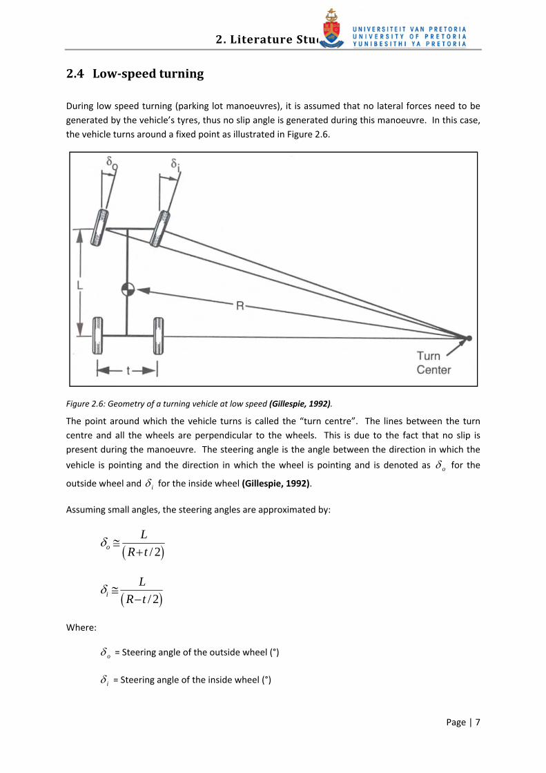
During low speed turning (parking lot manoeuvres), it is assumed that no lateral forces need to be generated by the vehicle’s tyres, thus no slip angle is generated during this manoeuvre. In this case, the vehicle turns around a fixed point as illustrated in Figure 2.6.
Figure 2.6: Geometry of a turning vehicle at low speed (Gillespie, 1992).
The point around which the vehicle turns is called the “turn centre”. The lines between the turn centre and all the wheels are perpendicular to the wheels. This is due to the fact that no slip is present during the manoeuvre. The steering angle is the angle between the direction in which the
vehicle is pointing and the direction in which the wheel is pointing and is denoted as oδ for the
outside wheel and iδ for the inside wheel (Gillespie, 1992).
Assuming small angles, the steering angles are approximated by:
( )/ 2oL
R tδ ≅
+
( )/ 2iL
R tδ ≅
−
Where:
oδ = Steering angle of the outside wheel (°)
iδ = Steering angle of the inside wheel (°)

2. Literature Study
Page | 8
L = Wheelbase (m)
R = Radius of the turn (m)
t = Track width (m)
The average steering angle is given by:
LR
δ =
This relationship is known as “Ackerman steering” or “Ackerman geometry”. This is the ideal steering angle of the “bicycle model” of the vehicle at low speeds. In the “bicycle model” the left and the right wheels are treated as one wheel with two times the vertical force on each wheel and two times the lateral force each wheel generated at the same slip angle. This means that no lateral load transfer and no body roll is taken into account in this two dimensional model (Gillespie, 1992).
2.5 High speed cornering
During high speed cornering, lateral acceleration on the vehicle cannot be neglected and plays a dominant role in handling dynamics. Thus, the tyres have to develop lateral forces to counteract the lateral acceleration. This means that slip angles will be generated at each wheel.
2.5.1 Tyre forces and the magic formula
The slip angle ( )α is the angle between the direction the vehicle is travelling in and the direction
the tyre is heading, as shown in Figure 2.7. The slope of this graph at the origin is known as the
cornering stiffness (Cα ).
Figure 2.7: Tyre cornering force properties (Gillespie, 1992).
2. Literature Study
Page | 9
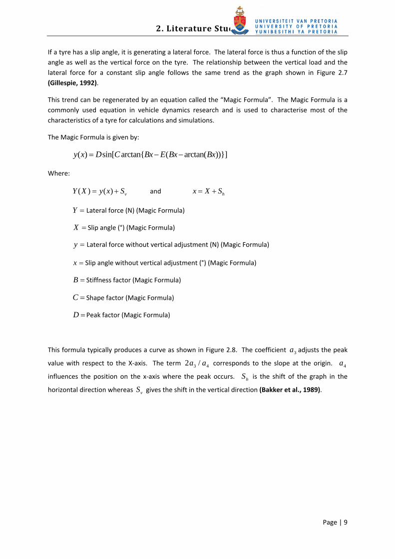
If a tyre has a slip angle, it is generating a lateral force. The lateral force is thus a function of the slip angle as well as the vertical force on the tyre. The relationship between the vertical load and the lateral force for a constant slip angle follows the same trend as the graph shown in Figure 2.7 (Gillespie, 1992).
This trend can be regenerated by an equation called the “Magic Formula”. The Magic Formula is a commonly used equation in vehicle dynamics research and is used to characterise most of the characteristics of a tyre for calculations and simulations.
The Magic Formula is given by:
( ) sin[ arctan{ ( arctan( ))}]y x D C Bx E Bx Bx= − −
Where:
( ) ( ) vY X y x S= + and hx X S= +
Y = Lateral force (N) (Magic Formula)
X = Slip angle (°) (Magic Formula)
y = Lateral force without vertical adjustment (N) (Magic Formula)
x = Slip angle without vertical adjustment (°) (Magic Formula)
B = Stiffness factor (Magic Formula)
C = Shape factor (Magic Formula)
D =Peak factor (Magic Formula)
This formula typically produces a curve as shown in Figure 2.8. The coefficient 3a adjusts the peak
value with respect to the X‐axis. The term 3 42 /a a corresponds to the slope at the origin. 4a
influences the position on the x‐axis where the peak occurs. hS is the shift of the graph in the
horizontal direction whereas vS gives the shift in the vertical direction (Bakker et al., 1989).

2. Literature Study
Page | 10
Figure 2.8: Typical shape of the Magic Formula representing the lateral tyre stiffness (Bakker et al., 1989).
The Magic Formula is defined in terms of coefficients 0a to 13a . To reconstruct the graph of the
lateral force vs. slip angle for a certain vertical load, the variables are used as follows to determine the coefficients of the Magic Formula: (Bakker et al., 1989).
ym zD Fμ=
Where:
1 2ym za F aμ = +
ymμ = Lateral friction coefficient
zF = Vertical force (N)
1a = Load dependency on lateral friction (Magic Formula)
2a = Lateral friction level (Magic Formula)

2. Literature Study
Page | 11
( )3 54
sin 2arctan 1zFBCD a aa
γ⎛ ⎞⎡ ⎤
= • −⎜ ⎟⎢ ⎥⎜ ⎟⎣ ⎦⎝ ⎠
Where:
γ = Chamber angle
3a =Maximum cornering stiffness (at 0γ = ) (Magic Formula)
4a = Load at maximum cornering stiffness (Magic Formula)
5a = Chamber sensitivity of cornering stiffness (Magic Formula)
0C a= (in this case, 0 1.3a = )
6 7zE a F a= +
E = Curvature factor (Magic Formula)
BCDBCD
=
8 9 10h zS a a F aγ= + +
11 12 13v z zS a F a F aγ= + +
6 13a a→ =Other Magic Formula coefficients
Only the information to construct the lateral force graph is given, but the same can be done for the longitudinal force and the self‐aligning torque.
2.5.2 Cornering equations
The steady state cornering equations for the bicycle model at high speeds are derived from
Newton’s second law ( )F ma= together with the equation describing the geometry in turns (Figure
2.9).
At high speeds, the turning circle is generally large, so the radius of the turn is large. This means that small angles can be assumed and that the steering angle of both the front wheels can be taken as equal.

2. Literature Study
Page | 12
Figure 2.9: Bicycle model during high speed cornering (Gillespie, 1992).
If a vehicle is travelling at a constant forward velocity of V , the sum of the forces in the lateral direction is given by (Gillespie, 1992):
2
y yf yrMVF F F
R= + =∑ [2‐1]
Where:
yF =Lateral force (N)
yfF = Lateral force on the front axle (N)
yrF = Lateral force on the rear axle (N)
M =Mass of the vehicle (kg)
V = Forward velocity (m/s)
R = Radius of the turn (m)
Because this is a steady‐state situation, the vehicle must be in force and moment equilibrium. Thus the moments about the centre of gravity (CG) equals zero. This states that:
0cg yf yrM F b F c= = −∑
Where b and c are the distances as denoted in Figure 2.9. Thus:
yf yr
cF Fb
=

2. Literature Study
Page | 13
This is substituted back into Equation [2‐1] to obtain:
2
1yr yr yrMV c b c LF F F
R b b b+⎛ ⎞ ⎛ ⎞ ⎛ ⎞= + = =⎜ ⎟ ⎜ ⎟ ⎜ ⎟
⎝ ⎠ ⎝ ⎠ ⎝ ⎠
Rearranging to make yrF the subject of the above equation gives:
2
yrMb VFL R
⎛ ⎞= ⎜ ⎟
⎝ ⎠
rW Mbg L
= is the portion of the vehicle mass on the rear axle. This means that lateral force
generated at the rear axle is given by the mass on the rear axle times the lateral acceleration at that point. Now the slip angles of the front and rear wheels can also be derived from Equation [2‐1] by
using yf f fF Cα α= and yr r rF Cα α= and rearranging so that α becomes the subject:
2
f ff
VWC gRα
α = [2‐2]
2
r rr
VWC gRα
α = [2‐3]
Now if the geometry of the model in Figure 2.9 is analysed and it can be seen that:
57.3 f rLR
δ α α= + − (in degrees) [2‐4]
Substituting Equation [2‐2] and [2‐3] into Equation [2‐4] gives:
2 2
57.3 f r
f r
W V W VLR C gR C gRα α
δ = + −
2
57.3 f r
f r
W WL VR C C gRα α
δ⎛ ⎞
= + −⎜ ⎟⎜ ⎟⎝ ⎠
[2‐5]
Where:
δ = Steering angle of the front wheels (°)
L =Wheelbase (m)
R =Radius of turn (m)
V = Forward speed (m/s)
2. Literature Study
Page | 14
g = Gravitational acceleration (9.81 m/s2)
fW = Load on the front axle (kg)
rW = Load on the rear axle (kg)
fCα = Cornering stiffness of the front tyres (kg/°)
rCα = Cornering stiffness of the rear tyres (kg/°)
2.5.3 Understeer gradient
Equation [2‐5] is often written in shorthand form as follows:
57.3 y
L KaR
δ = +
Where:
K =Understeer gradient (°/g)
ya =Lateral acceleration (g)
Equation [2‐5] clearly shows the influence of different parameters on the required steering angle.
The term [ / / ]f f r rW C W Cα α− determines the magnitude and direction of the steering input
required. It consists of two terms, each of which is the ratio of the load on the wheels to the
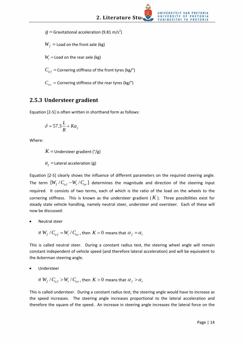
cornering stiffness. This is known as the understeer gradient ( K ). Three possibilities exist for steady state vehicle handling, namely neutral steer, understeer and oversteer. Each of these will now be discussed:
• Neutral steer
If / /f f r rW C W Cα α= , then 0K = means that f rα α=
This is called neutral steer. During a constant radius test, the steering wheel angle will remain constant independent of vehicle speed (and therefore lateral acceleration) and will be equivalent to the Ackerman steering angle.
• Understeer
If / /f f r rW C W Cα α> , then 0K > means that f rα α>
This is called understeer. During a constant radius test, the steering angle would have to increase as the speed increases. The steering angle increases proportional to the lateral acceleration and therefore the square of the speed. An increase in steering angle increases the lateral force on the
2. Literature Study
Page | 15
front tyres to keep the sum of the moments around the CG point zero. This trend for the front of the vehicle to drift outwards is compensated for by increasing the steering angle.
• Oversteer
If / /f f r rW C W Cα α< , then 0K < means that f rα α<
This is called oversteer. During a constant radius test, the steering angle would have to decrease as the speed increases. The steering angle decreases proportional to the lateral acceleration and therefore the square of the speed. A decrease in steering angle reduces the lateral force on the front tyres to keep the sum of the moments around the CG point zero. The rear of the vehicle tends to drift outwards and is compensated for by decreasing the steering angle. If the speed increases even further, counter steering can become necessary to keep the vehicle to follow the desired path (Gillespie, 1992).
The effect of neutral‐, over‐ and understeering is shown in Figure 2.10.
Figure 2.10: Change of steering angle with speed for vehicles with different steering characteristics (Gillespie, 1992).
2.5.4 Roll moment distribution
During high speed cornering, lateral acceleration is generated that affects the vehicle. According to
Newton’s second law, this imposes a lateral force ( )yF on the CG point. Due to the fact that the
height of CG ( )CGh is generally more than the height of the roll centre ( )rh on a standard vehicle,

2. Literature Study
Page | 16
the lateral force imposes a moment around the roll centre. This results in the body leaning to the outside during turning. This situation is shown in Figure 2.11.
Figure 2.11: Force analysis of a vehicle during cornering (Gillespie, 1992).
This result in the vertical loads on the inside wheels decreasing and on the outside wheels increasing by the same amount. Due to the fact that the relationship between the lateral force and the vertical load is a non‐linear relationship (Figure 2.12), the change in vertical load between the inside and outside wheels of the vehicle results in less lateral force that can be generated. Increasing the lateral load transfer (e.g. by using stiff springs or an anti‐roll bar) decreases the lateral force that can be generated by the tyres (Gillespie, 1992).
This is one of the reasons why a Winston cup race car is built asymmetric by means of moving the CG point to the inside of the vehicle. This results in the vertical load on the tyres being equal during cornering at a specific speed on the oval track. This increases the amount of lateral force the tyres can generate and allows the vehicle to increase its cornering speed (Haubenreich and Law, 2000).
This lateral load transfer can also play a role in the over‐ or understeer characteristics of the vehicle. If the front of the vehicle experiences more lateral load transfer than the rear wheels, the lateral force that can be generated by the front tyres will decrease. The slip angle at the front tyres will have to be increased to compensate for this, by increasing the steering angle. The vehicle will therefore tend to understeer. Similarly, if the rear of the vehicle experiences more lateral load transfer than the front wheels, the vehicle will tend to oversteer.

2. Literature Study
Page | 17
Figure 2.12: Vertical force vs. vertical load characteristic of the tyre (Gillespie, 1992).
To determine if a vehicle will slide before it will roll on a flat road the sum of the moments around the point of rotation during rollover is investigated. During rollover, the vehicle rotates around the contact point of the outside wheel. With reference to Figure 2.11, the sum of the moments around this point during cornering, if steady state conditions and rigid suspension is assumed, is given by:
0
02
2
O
y CG
y CG
MtMg Ma h
tMg Ma h
∑ =
⎛ ⎞− =⎜ ⎟⎝ ⎠⎛ ⎞ =⎜ ⎟⎝ ⎠
Thus, 2
y
CG
a tg h= [2‐6]
Where:
OM = Moments about the contact patch of the outside wheel (Nm)
t = Track width (m)
CGh = Height of CG point (m)

2. Literature Study
Page | 18
/ya g in Equation [2‐6] represents the magnitude of the lateral acceleration where the vertical
force on the inside wheel ( ziF ) is zero and is called the rollover threshold. To ensure that the
vehicle will always slide instead of roll, the following relation must hold:
2
y
CG
a tg h<
[2‐7]
From Newton’s second law ( )F ma= , ya can be written as:
yF Ma= [2‐8]
The force ( )F is the friction force between the tyres and the road. The maximum friction force is
given by:
maxF Mgμ= [2‐9]
Where:
μ = Friction coefficient between the tyres and the road
If Equation [2‐8] and [2‐9] is substituted into Equation [2‐7], the following relationship is obtained:
2 CG
th
μ < [2‐10]
This relationship in Equation [2‐10] states that if the track width divided by two times the CG height is larger than the friction coefficient of the road, the vehicle will slide before it will roll. The right hand side of this equation is known as the static stability factor (SSF) and is given as (Forkenbrock et. al., 2004):
2 CG
tSSFh
=
From this theoretical analysis of the lateral dynamics of a simplified linear vehicle model, it can be concluded that for improving the handling capabilities of a vehicle, the lateral acceleration that can be generated by the vehicle must be increased. But if the lateral acceleration is taken as the optimising variable, the μ in Equation [2‐10] will increase, which will result in the vehicle rolling
before sliding. This situation is undesirable, because it compromises the safety of the vehicle. This is the case with most vehicles with high CG’s such as SUVs.
Uys et. al. (2004) conducted a study on what parameter(s) should be used to quantify and optimise the handling of a vehicle. The tests strongly suggested that roll angle is a suitable variable to quantify handling. It is also suitable for the optimisation of suspension settings given a prescribed road and manoeuvre.

2. Literature Study
Page | 19
From this, it is concluded that the roll angle will be used to quantify and optimise the handling of the vehicle. It must be kept in mind that reducing the roll angle during a handling manoeuvre increases the roll stiffness of the vehicle, which increases the vertical load transfer on the tyres. This will result in a lower lateral force that can be generated by the tyres, thereby reducing the μ in Equation [2‐
10]. In other words, optimising the roll angle off the vehicle improves the safety and reduces the roll over tendency of the vehicle.
Optimising the roll angle during a handling manoeuvre can be achieved by one of the following three methods:
1. Lower the CG point of the vehicle. If the CG point is lowered, the distance between the roll centre and the CG of the vehicle decreases. This decreased distance decreases the moment about the roll centre due to the mass of the vehicle, when the vehicle experiences lateral acceleration. Due to the decreased moment, the roll angle of the vehicle body will decrease which will decrease the vertical load transfer on the tyres. The lower CG height will increase the SSF, increasing the tendency of the vehicle to slide before it will roll. A lower CG point can be obtained by semi‐active, slow‐active or active suspension systems.
2. Increase the suspension stiffness and/or damping. By increasing the suspension stiffness, the vehicle’s steady state cornering will improve and by increasing the suspension damping, the vehicle’s dynamic handling improves. This is due to the fact that increasing the suspension stiffness and/or damping reduces the body roll of the vehicle. This reduction in body roll increases vertical load transfer on the tyres and decreases the total available side forces at each axle. The suspension stiffness and/or damping can be increased by passive, semi‐active or active suspension systems.
3. An additional system can be added to increase the roll stiffness of the vehicle. This will increase the vertical load transfer on the tyres and decreases the total available side forces at each axle. These systems are for instance semi‐active and active anti‐roll bars, semi‐active suspension and active suspension.

2. Literature Study
Page | 20
2.6 Proposed solutions
Quite a number of solutions were found in literature for improving vehicle handling. These solutions will now be discussed:
2.6.1 Passive suspension
Wilde et al. (2005) presented results from simulation and testing of the Kinetic suspension system, a passive interconnected suspension system. It consists of four hydraulic cylinders, two accumulators and connection pipes. This system counters body roll during handling manoeuvres (Figure 2.13) and vehicle articulation (Figure 2.14). It was tested on a Honda CRV by means of the NHTSA fishhook manoeuvre. The maximum speed the vehicle can manage without lifting two wheels two inches from the ground or a rim touching the ground was measured and used to determine the performance of the system. This system improved the vehicle’s speed in the fishhook manoeuvre from 43 mph to more than 60 mph.
Figure 2.13: Kinetic system during body roll (Wilde et al., 2005).
2. Literature Study
Page | 21
Figure 2.14: Kinetic system during vehicle articulation (Wilde et al., 2005).
2.6.2 Four state semiactive suspension system (4S4)
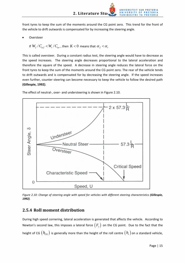
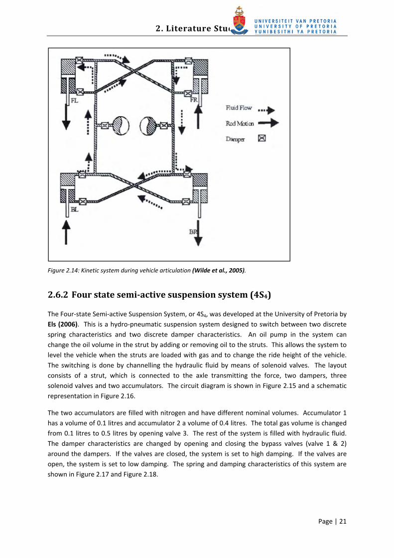
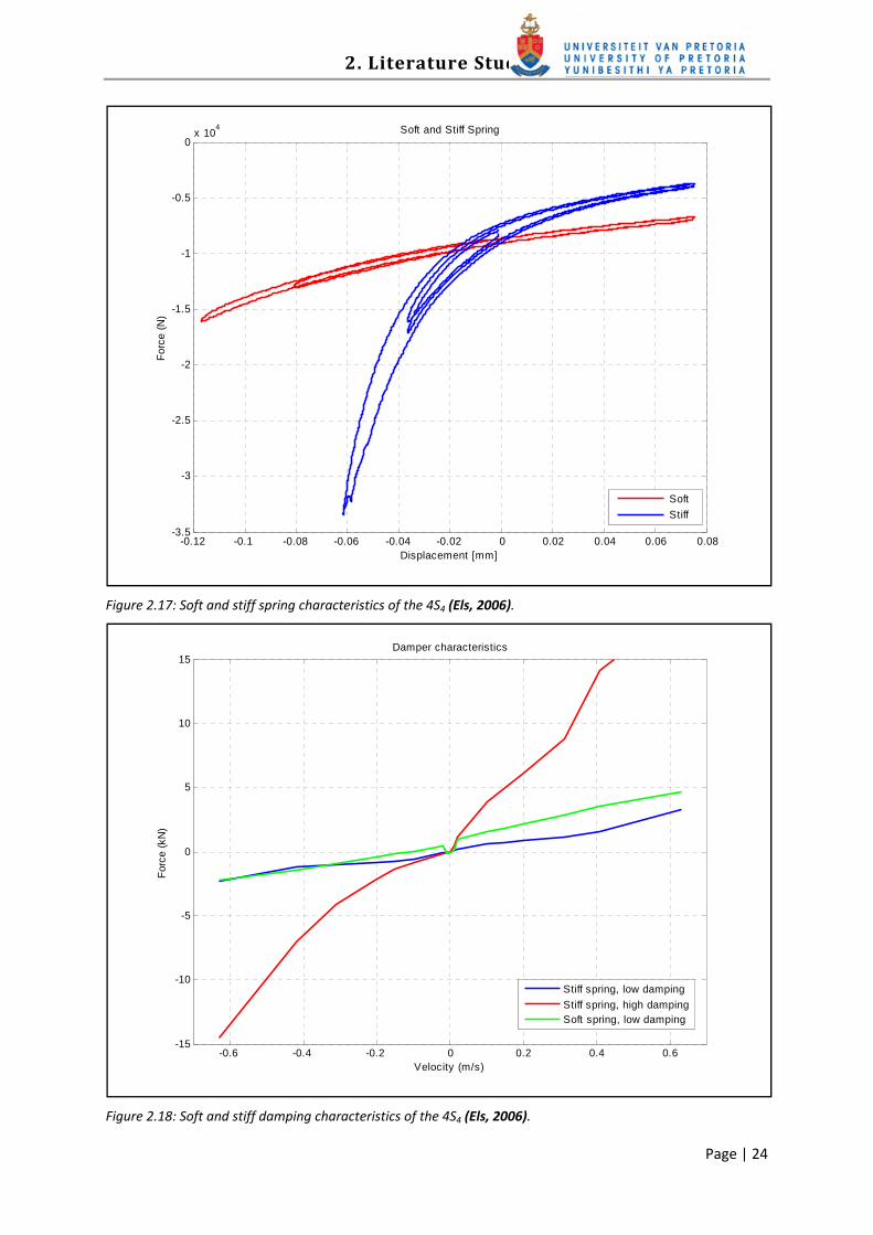
The Four‐state Semi‐active Suspension System, or 4S4, was developed at the University of Pretoria by Els (2006). This is a hydro‐pneumatic suspension system designed to switch between two discrete spring characteristics and two discrete damper characteristics. An oil pump in the system can change the oil volume in the strut by adding or removing oil to the struts. This allows the system to level the vehicle when the struts are loaded with gas and to change the ride height of the vehicle. The switching is done by channelling the hydraulic fluid by means of solenoid valves. The layout consists of a strut, which is connected to the axle transmitting the force, two dampers, three solenoid valves and two accumulators. The circuit diagram is shown in Figure 2.15 and a schematic representation in Figure 2.16.
The two accumulators are filled with nitrogen and have different nominal volumes. Accumulator 1 has a volume of 0.1 litres and accumulator 2 a volume of 0.4 litres. The total gas volume is changed from 0.1 litres to 0.5 litres by opening valve 3. The rest of the system is filled with hydraulic fluid. The damper characteristics are changed by opening and closing the bypass valves (valve 1 & 2) around the dampers. If the valves are closed, the system is set to high damping. If the valves are open, the system is set to low damping. The spring and damping characteristics of this system are shown in Figure 2.17 and Figure 2.18.

2. Literature Study
Page | 22
Figure 2.15: Circuit diagram of the 4S4 (Els, 2006).
The reason for the spring characteristics not being linear is because the spring force is generated by compressing a gas. This means that the ideal gas law can be assumed and is given by:
PV nRT=
Where:
P = Pressure (Pa )
V = Volume ( 3m )
n =Amount of moles of gas (mol )
R = Universal gas constant 1 18.314 . .J mol K− −=
T = Temperature (K )
This shows that the relationship between the pressure and the volume is given by 1PV
∝ which is
a hyperbolic relationship.

2. Literature Study
Page | 23
Figure 2.16: Schematic representation of the 4S4 (Els, 2006).
2. Literature Study
Page | 24
Figure 2.17: Soft and stiff spring characteristics of the 4S4 (Els, 2006).
Figure 2.18: Soft and stiff damping characteristics of the 4S4 (Els, 2006).
-0.12 -0.1 -0.08 -0.06 -0.04 -0.02 0 0.02 0.04 0.06 0.08-3.5
-3
-2.5
-2
-1.5
-1
-0.5
0x 104 Soft and Stiff Spring
Displacement [mm]
Forc
e (N
)
SoftStiff
-0.6 -0.4 -0.2 0 0.2 0.4 0.6-15
-10
-5
0
5
10
15
Velocity (m/s)
Forc
e (k
N)
Damper characteristics
Stiff spring, low dampingStiff spring, high dampingSoft spring, low damping
2. Literature Study
Page | 25
Various simulations and tests were done by Els (2006) to determine the optimised values for the spring and damper characteristics. It was found that for the best possible handling, a stiff spring is required (0.1 litre static gas volume for hydro pneumatic spring in the case of the test vehicle) and for optimum ride comfort a soft spring is required (>0.5 litre static gas volume for hydro pneumatic spring in the case of the test vehicle). For the damping characteristics, it was found that high damping is required for handling (more than double the base line damping) and low damping for ride comfort (less than half the base line damping value). The 4S4 was designed to meet these optimised characteristics.
This system can switch from one suspension setting to the other within 100 milliseconds by switching the solenoid valves. The system autonomously decides which setting to choose. This decision is made by taking the running RMS (RRMS) between the lateral and vertical acceleration of the vehicle body. If the vertical RRMS is larger than the lateral RRMS, the system switches to the ride comfort setting and vice versa. The system can also be forced to stay on the handling (stiff spring, high damping) or the ride comfort (soft spring, low damping) setting by toggling a switch on the dash board.
This system has been thoroughly tested and has shown during a DLC (double‐lane‐change) manoeuvre at 70 km/h that the handling setting reduced the maximum body roll angle by 78% over the factory vehicle and by 90% over the ride comfort setting. The ride comfort setting performed similarly as the factory vehicle and showed a 50% to 80% improvement in ride comfort over the handling setting on Belgian paving (Els, 2006).
2.6.3 Other semiactive suspension systems
Semi‐active suspension systems and more specifically semi‐active dampers are often used for ride comfort improvements. Ahmadian and Simon (2004) implemented and tested Skyhook control and steering input augmented (SIA) skyhook control on a 2000 Ford Expedition SUV. The vehicle was fitted with magneto‐rheological semi‐active dampers to control the damping of the suspension. The test manoeuvre was a swerve test where the vehicle is driven in a straight lane, swerves out for an obstacle and continues in the original lane. This test was done at a speed of 20 mph (33 km/h). The pitch and roll acceleration were used as quantifying variables during this swerve test. The test results showed that the Skyhook control and the SIA skyhook control gave more than a 10% improvement on roll and pitch acceleration over the standard passive suspension.
Kim et al. (2005) describe Mando’s continuously semi‐active suspension system (SDC‐20 model). This system controls the damping of the suspension between two settings by means of variable hydraulic dampers. The variable damping is used to control the response of the vehicle body during handling manoeuvres, severe road irregularities, nosedive, squat, yaw, pitch and heave. Different settings are also available such as auto, sport and comfort to change the ride experience. The aim of the design was firstly to optimise the design of the control valve and to keep it compact and light with fast response and secondly to enhance the control performance, functionality, handling and safety aspects in co‐operation with ESP (electronic stability program). Only simulations are presented for the results of this system. A handling simulation was done where a single cycle sinusoidal sweep with amplitude of 90° is given to the steering wheel. The roll velocity of the vehicle

2. Literature Study
Page | 26
is taken as the measuring variable. The SDC‐20 system showed up to a 50% improvement in peak roll velocity during the described test.
Yoon et al. (2006) evaluated the efficiency of CDC (continuous damping control), ESP (electronic stability program) and UCC (unified chassis control) to prevent rollover of SUVs. UCC is a combination of CDC and ESP. In effect, it uses the CDC to improve the effect of ESP. A model was built in ADAMS/Car and verified by means of a step steer manoeuvre against measured results of the real vehicle. Each system was then implemented and evaluated by doing a fishhook test and determining the speed at which rollover occurred. Rollover was defined as the occurrence when two wheels lift two inches from the ground. The results showed that CDC posed almost no improvement; ESP gave a 25% improvement in speed and UCC more than a 50% improvement in the speed, compared with the conventional vehicle.
2.6.4 Active antiroll bars
Anti‐roll bars control the roll stiffness of the vehicle independent of vertical (ride) stiffness. This allows the anti‐roll bar to control the body roll angle of the vehicle as well as the vertical load transfer between the left and the right wheels. Active anti‐roll bars consist of an anti‐roll bar and an actuator to increase the effect of a passive anti‐roll bar. This allows the anti‐roll bar to act on the vehicle only when needed.
Everett et al. (2000) investigated the use of an active anti‐roll bar for SUVs. This was done by means of actuating an anti‐roll bar with a hydraulic cylinder, which was controlled by an open loop control system directly proportional to the lateral acceleration of the vehicle. Only simulations were done during this study. Three tests were conducted: the steady state cornering test, moderate ramp input test and severe ramp input test. All the tests were done with only the driver in the vehicle as well as with a fully loaded vehicle. The handling of the vehicle was quantified by measuring the body roll angle of the vehicle during the tests. The results of the steady state cornering test showed a 55% improvement for the vehicle with the driver only and a 24% improvement for the loaded vehicle. The moderate ramp input test showed a 70% improvement for the vehicle with the driver only and a 33% improvement for the loaded vehicle, where the severe ramp input test also showed a 70% and a 31% improvement for the two cases. Different results where obtained by moving the accelerometer that measures the lateral acceleration further in front of the CG point. The optimal distance was 0.75 m in front of the CG point. All the tests were done with the accelerometer at the optimal position. The system was designed so that the vehicle had an almost 0° roll angle up to a lateral acceleration of 0.4 g. If the lateral acceleration increases even further, the roll angle increases at the same rate as the passive system. This was done to warn the driver that the lateral acceleration on the vehicle is approaching the vehicle’s friction limit.
Darling et al. (1992) developed a low cost active anti‐roll suspension for passenger cars. This suspension system consisted of two anti‐roll bars (one at the back and one at the front) actuated by two hydraulic cylinders. The hydraulic cylinders are controlled directly proportional to the lateral acceleration as measured at the CG point of the vehicle. Only simulations were done in this study. A step steer test was done with a steering wheel input of 30 degrees at a speed of 22.2 m/s (80 km/h). The body roll angle was measured to quantify the performance of the vehicle during the test. This
2. Literature Study
Page | 27
test showed an 82% improvement between the passive and active systems. It was also shown that this system improves the tyre camber during the test by 34%, which improves the cornering properties of the tyre.
Darling and Hickson (1998) designed an active anti‐roll bar system, which consisted of two anti‐roll bars actuated by means of two hydraulic actuators. Simulations were done to predict the response of the system. Finally the system was fitted to a Ford Fiesta Mark II to verify the simulations. Two tests were done. The first test was a steady state handling test, where the vehicle speed was increased while a constant steering angle was maintained. During this test, the lateral acceleration on the vehicle ranged from 0.5 – 8 m/s2. The second test was a dynamic handling test. During this test, the vehicle was driven at constant speed and a step input was applied to the steering wheel of magnitudes 90°, 180°, 270° and 360°. The handling performance of the vehicle was rated by measuring the body roll angle of the vehicle during the test manoeuvres. The results showed an improvement in body roll during the steady state test of over 80% and an improvement in the peak body roll angle during the dynamic handling test of approximately 80%.
Cimba et al. (2006) developed an active torsion bar system, which consists of an anti‐roll bar actuated by a hydraulic cylinder. The system was designed to eliminate body roll up to a lateral acceleration of 0.5g and when no roll control is needed, the hydraulic cylinder is released so that the single wheel irregularities are not amplified by the torsion bar. Simulations were done and then the system was built to verify the simulations. Three tests were conducted to determine the response of the system and to test the maximum hose length of the hydraulic system before it has a considerable effect on the system. These tests were step steer tests, fishhook tests and slalom tests. The performance of the vehicle was quantified by measuring the body roll angle of the vehicle during the tests. The system showed an overall improvement of 73% in body roll angle and it was determined that a maximum hose length of 24 m could be used before it influences the response of the system.
Danesin et al. (2003) designed an active roll control system to increase handling and comfort. This system consisted of two anti‐roll bars, which is each actuated by a hydraulic actuator. Simulations were done and the system was tested on an Alfa Romeo 166 – 3.0 V6. Two tests were conducted to test the response of the system. The first was a sine sweep test where the vehicle speed is kept constant and a sine input is given to the steering wheel. The second test was a step steer test where a constant speed is again maintained and a step input is given to the steering wheel. The side slip angle and the yaw rate of the vehicle was used to quantify the performance of the vehicle during the tests. The system showed a 20% improvement in the yaw rate and a 45% peak improvement in the side slip angle during the step steer test at 100 km/h with a step steering input of 100° over the baseline vehicle.
Sorniotti (2006) developed an electro‐mechanical active roll control system that consists of two anti‐roll bars actuated by two electro‐mechanical torque actuators. Electronic stability control (ESC) was also used to test its influence on the vehicle in conjunction with the active roll control system. Simulations as well as experimental tests were conducted. The system was tested by means of an extreme step steer manoeuvre and the body roll angle as well as the yaw rate was used to determine the performance of the system. During this test, the body roll angle of the vehicle was

2. Literature Study
Page | 28
improved by 33% with the active roll control system and by 42% with the active roll control system with ESC.
Kim and Park (2004) designed a robust roll motion control system. This system consists of two anti‐roll bars actuated by two linear electro‐mechanic actuators. The system was controlled by a closed loop control system, which uses the lateral acceleration of the vehicle as input. The hardware in the loop method was used to simulate the system. A test bench was built to test the anti‐roll bar system and determine its characteristics, which are inserted in the simulation. The test manoeuvre used is a step steer manoeuvre. The body roll angle was used to quantify the performance of the system. This system showed an 85% improvement in the body roll angle during the step steer manoeuvre at 50 km/h and a 73% improvement in the same manoeuvre at 100 km/h. Finally it was mentioned that the use of a hybrid control with variable dampers in conjunction with an active anti‐roll system will produce even better results.
2.6.5 Active suspension
Packer (1978) proposed a hydro‐pneumatic suspension as well as two methods of slow actively controlling the suspension to improve handling. The first method entails interlinking the hydraulic cylinders to counter body roll. The second method is a self‐levelling mechanism, which automatically adds or dumps oil to and from the system (Figure 2.19). Only the second system was investigated. A theoretical model of the system was created and results were predicted before the system was tested. Two tests were performed. The first was a cornering test up to the point where the vehicle experienced a lateral acceleration of 0.5 g before returning to a straight line. The second test was a braking test where the vehicle drives in a straight line and brakes up to a 0.5 g longitudinal acceleration. For both tests, the suspension displacement was measured for the vehicle with and without this system. During the first test, this system showed a 70% improvement in suspension displacement and 77% for the front wheels during the second test. The problem with this system is that it might be activated by a bump on a rough road, which is highly undesirable. The most interesting part of this system is that it is a completely mechanical system with no electronics.
Figure 2.19: Schematics of proposed solution by Packer (1978).

2. Literature Study
Page | 29
Tillback and Brodd (1989) describe an active suspension system that improves handling, ride comfort and safety. The system is controlled by a closed loop double feedback control system, which takes the steering angle, yaw rate, longitudinal acceleration, lateral acceleration and vertical acceleration into account. These input signals are then used in an algorithm to decide how to respond to the current situation to obtain optimal handling performance. The safety is improved by reducing roll angles, reducing tyre vertical force variation, reducing vertical body overshoot and controlling vertical force distribution. Unfortunately, no test procedure or results are given in this article. This is only a documentary study.
Shuttlewood et al. (1993) proposed a non‐linear model of a hydro‐pneumatic suspension system. The suspension struts are actuated by moving oil between the accumulators and the struts by means of a hydraulic pump. The control system uses the lateral acceleration to determine the desired response of the system. Only simulations were done to acquire results and no actual test to verify the results. A J‐manoeuvre is simulated up to a lateral acceleration of 0.8 g. The body roll angle was measured to quantify the handling of the vehicle. One of the problems experienced is that the roll movement of the body shows low damping and oscillates when the vehicle enters the turn. This can be reduced by moving the accelerometer forward by a distance of 0.6 m in front of the CG. The simulations showed that the system improves the body roll angle by up to 80% during the J‐turn manoeuvre.
Darling and Rosam (1996) used a hydro‐pneumatic suspension system on which an active roll control system was implemented. This was done by transferring hydraulic fluid from one side to the other, depending on which side the body is rolling to, by means of a hydraulic pump. The system was designed so that body roll was eliminated up to a lateral acceleration of 0.35g and then increased at the same rate as the passive vehicle. The experimental tests confirmed that the system consumes modest power and should be ‘failsafe’ without affecting the vehicle’s handling behaviour. The whole system was simulated and tested on a Rover 100. A step steer manoeuvre with a steering input of 90° was done at a speed of 13 m/s (47 km/h) to measure the performance of the system. The performance of the system was quantified by measuring the body roll angle of the vehicle during the step steer manoeuvre. The tests showed an improvement in maximum body roll angle of 75% between the test vehicle with and without this active suspension system.
Hubert and Kumar (2005) describe an active suspension system which actively changes the damping of the suspension. The control system uses 13 sensors to monitor the vehicle’s situation and an algorithm calculates the desired damping force. All of this is done in a single microprocessor and has a reaction time of 2.5 milliseconds. This is only a documentation study, so no simulations or tests are described in this article.
2.6.6 Tilting vehicles
Gohl et al. (2004) investigated steering tilt control (STC), which was implemented on a narrow tilting vehicle (NTV) (Figure 2.20). These vehicles lean into the turn during cornering. This shifts the CG point of the vehicle to the inside of the turn, which decreases the moment about the outside wheel, decreasing the chances for roll‐over. The system was modelled in Matlab and Visual Basic and then an experimental model was built to verify the simulations. The results showed that STC improved

2. Literature Study
Page | 30
the stability of the vehicle, but the amount of improvement is not given. It was also stated that this principle works better on narrow vehicles than wider vehicles.
Figure 2.20: Narrow tilting vehicle (Gohl et al. 2004).
2.6.7 Selection of proposed solutions
A number of proposed solutions found in the literature have been discussed. A set of criteria has been set up by which the proposed solutions will be weighted to determine the most suitable solution. These criteria are:
1. Is this solution feasible on a SUV? 2. Will this solution be able to function effectively in a rugged off‐road environment? 3. What is the given improvement for this solution in the literature? 4. Can this solution improve other aspects of the vehicle as well? 5. What is the energy consumption of this solution? 6. Can this solution be added to or incorporated in the current 4S4?
Each question in the criteria is awarded a weighting according to the importance it has in the choosing of the most suitable solution. Each solution is then given a mark out of 10 for each question. The given mark is then multiplied by the weighting and all the weighted marks are added together for each solution. This weighting process is shown in Table 3. The solutions taken from the literature are the following:
1. Passive interconnected suspension system as given by Wilde et al. (2005). 2. 4S4 as described by Els (2006). 3. Variable damping semi‐active suspension system as given by Ahmadian and Simon. (2004),
Kim et al. (2005) and Yoon et al. (2006).
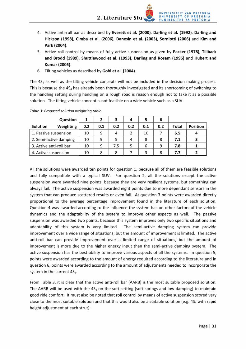
2. Literature Study
Page | 31
4. Active anti‐roll bar as described by Everett et al. (2000), Darling et al. (1992), Darling and Hickson (1998), Cimba et al. (2006), Danesin et al. (2003), Sorniotti (2006) and Kim and Park (2004).
5. Active roll control by means of fully active suspension as given by Packer (1978), Tillback and Brodd (1989), Shuttlewood et al. (1993), Darling and Rosam (1996) and Hubert and Kumar (2005).
6. Tilting vehicles as described by Gohl et al. (2004).
The 4S4 as well as the tilting vehicle concepts will not be included in the decision making process. This is because the 4S4 has already been thoroughly investigated and its shortcoming of switching to the handling setting during handling on a rough road is reason enough not to take it as a possible solution. The tilting vehicle concept is not feasible on a wide vehicle such as a SUV.
Table 3: Proposed solution weighting table.
Question 1 2 3 4 5 6
Solution Weighting 0.2 0.1 0.2 0.2 0.1 0.2 Total Position
1. Passive suspension 10 9 4 2 10 7 6.5 4 2. Semi‐active damping 10 9 5 4 8 8 7.1 3 3. Active anti‐roll bar 10 9 7.5 5 6 9 7.8 1
4. Active suspension 10 8 8 7 3 8 7.7 2
All the solutions were awarded ten points for question 1, because all of them are feasible solutions and fully compatible with a typical SUV. For question 2, all the solutions except the active suspension were awarded nine points, because they are very resilient systems, but something can always fail. The active suspension was awarded eight points due to more dependant sensors in the system that can produce scattered results or even fail. At question 3 points were awarded directly proportional to the average percentage improvement found in the literature of each solution. Question 4 was awarded according to the influence the system has on other factors of the vehicle dynamics and the adaptability of the system to improve other aspects as well. The passive suspension was awarded two points, because this system improves only two specific situations and adaptability of this system is very limited. The semi‐active damping system can provide improvement over a wide range of situations, but the amount of improvement is limited. The active anti‐roll bar can provide improvement over a limited range of situations, but the amount of improvement is more due to the higher energy input than the semi‐active damping system. The active suspension has the best ability to improve various aspects of all the systems. In question 5, points were awarded according to the amount of energy required according to the literature and in question 6, points were awarded according to the amount of adjustments needed to incorporate the system in the current 4S4.
From Table 3, it is clear that the active anti‐roll bar (AARB) is the most suitable proposed solution. The AARB will be used with the 4S4 on the soft setting (soft springs and low damping) to maintain good ride comfort. It must also be noted that roll control by means of active suspension scored very close to the most suitable solution and that this would also be a suitable solution (e.g. 4S4 with rapid height adjustment at each strut).

2. Literature Study
Page | 32
2.7 Conclusion
The following is concluded based on the evidence provided in this chapter:
• From the theory, it was taken that one or more of the following steps can by taken to improve the handling capabilities of a vehicle:
o Lower the CG point of the vehicle. o Increase the suspension stiffness and/or damping. o Add an additional system to increase vertical load transfer on the tyres.
• The literature showed a wide variety of solutions that address the problem statement.
• All the solutions found in the literature were weighted against the given criteria in order to determine the most suitable solution for the problem statement. The active anti‐roll bar solution was shown to be the most suitable solution and will be implemented in the rest of this study.
• As it was decided to focus on the problem of improving the handling of the vehicle without sacrificing ride comfort on rough roads, the solution generated was to use the soft suspension of the 4S4 (soft springs and low damping) to absorb the irregularities in the road and control body roll with an active anti‐roll bar (AARB).

Page | 33
3 Simulations
Simulations were used to test the feasibility of the proposed solution, predict the results of the system and obtain some key design parameters. In this chapter the simulation model will be discussed followed by the road type and manoeuvres performed. The parameters which were altered to verify and improve the model will be mentioned and finally the simulations that will be done to test the proposed solution are presented.
3.1 Simulation model
ADAMS/View 2005 was used to build and simulate a model of the Land Rover Defender 110. This is a full vehicle model and has 15 unconstrained degrees of freedom. The ADAMS/Controls interface was used to link ADAMS/View with Matlab 7.0.1 and Simulink 6.1. This software interaction is illustrated graphically in Figure 3.1. It was done by exporting predefined variables to Simulink. These variables are used to do calculations in Simulink and Matlab. The calculated values are sent back to ADAMS to be used in the simulation. Vehicle dynamics were solved in ADAMS while spring characteristics, damper characteristics and AARB characteristics and control were calculated in Matlab and Simulink.
Figure 3.1: Simulation interaction.
An existing full vehicle model was used as developed by Thoresson (2007) and Uys (2007). This model was built based on the properties of a Land Rover Defender 110, which was also used for the experimental tests. The geometric dimensions were measured or taken from technical drawings of the components. The roll, pitch and yaw moments of inertia as well as the CG point was determined by experimental measurements as described by Uys et al. (2006). The test vehicle and simulation model uses the 4S4 as described in paragraph 2.6.2. A graphic representation of this model is shown in Figure 3.2.
The characteristics of the bump‐stops, 4S4 hydro‐pneumatic springs and dampers were measured on Shenck Hydropulse test equipment. Theoretical models of these characteristics were then

3. Simulations
Page | 34
implemented in Matlab. The lateral tyre characteristics were measured by means of a two‐tyre testing rig that is towed behind a vehicle and measures the lateral force. This was done for slip angles up to 10° and at vertical loads of 400 kg, 850 kg and 1300 kg. This data was modelled with the Pacejka ’89 tyre model, which is used in the simulation model (Bakker et al., 1989). The tyre data is shown in Figure 3.3.
Figure 3.2: ADAMS/View model used for the simulations.
The front suspension is modelled by means of a rigid axle, which is fixed longitudinally by two leading arms connected to the body with rubber bushes. The stiffness of these bushes was measured and modelled in the ADAMS model. The rigid axle is fixed laterally with a Panhard rod. Figure 3.4 shows the layout in ADAMS while Figure 3.5 gives a schematic layout indicating the different bodies with their connecting joints.
The rear suspension also consists of a rigid axle with two trailing arms. An A‐arm connected with a revolute joint to the body and a spherical joint to the axle fixes the axle in the lateral direction. The stiffness of the trailing arm rubber bushes is also included in the simulation model. Figure 3.6 shows the layout in ADAMS while Figure 3.7 gives a schematic layout indicating the different bodies and connecting joints. The modelling of the ARB (anti‐roll bar) will be discussed in paragraph 3.4.

3. Simulations
Page | 35
Figure 3.3: Tyre side force vs. slip angle characteristics (Els, 2006).
Figure 3.4: Front suspension modelled in ADAMS (Els, 2006).

3. Simulations
Page | 36
Figure 3.5: Schematic of front suspension model.

3. Simulations
Page | 37
Figure 3.6: Rear suspension modelled in ADAMS (Els, 2006).

3. Simulations
Page | 38
Figure 3.7: Schematic of rear suspension model.

3. Simulations
Page | 39
3.2 Road type and manoeuvres
Handling simulations were done on a flat smooth road with the characteristics of a concrete road in good condition. Ride comfort simulations were done on the Belgian paving as found at Gerotek (Gerotek Test Facilities, 2008). This is a 5 m x 100 m stretch of paved stones as shown in Figure 3.8. Simulations were also performed where handling was simulated on the Belgian paving.
Figure 3.8: Belgian paving on suspension track at Gerotek (Gerotek Test Facilities, 2008).
A constant radius test and a DLC test were performed on the flat concrete road to determine the steady state and dynamic handling ability of the vehicle. A ride comfort test was done by driving over the Belgian paving in a straight line at constant speed as well as a DLC manoeuvre. The test on the Belgian paving was done to determine the influence of the system on ride comfort. The DLC manoeuvre was done to determine the dynamic handling on a rough road. Unfortunately, there is not a wide enough Belgian paving available to do an experimental DLC manoeuvre on, therefore only simulation results could be obtained. The data of the Belgian paving was copied and added together to create a big enough area to simulate a DLC manoeuvre. A graphical representation of this simulation is shown in Figure 3.9.
A three‐dimensional road profile of the Belgian paving was created by Becker (2008) by building a platform driving over the Belgian paving with fingers measuring the vertical displacement of the road (Figure 3.10). This data was then converted in Matlab to give the representation as shown in Figure 3.11 that could be used in ADAMS simulations. Becker (2008) used the same simulation model of the Land Rover used in this study to validate the model for ride comfort over the Belgian paving.

3. Simulations
Page | 40
Figure 3.9: Belgian paving used in simulations to perform a DLC manoeuvre.
Figure 3.10: Fingers measuring the surface profile of the Belgian paving (Becker, 2008).

3. Simulations
Page | 41
Figure 3.11: Electronic format of the Belgian paving (Becker, 2008).
Simulation results on this digital representation of the Belgian paving shows an average difference in the weighed RMS values of the vertical acceleration of 22% at a speed of 40 km/h compared to the measured results. The percentage difference between the measured and simulated weighted RMS are given in Figure 3.12. This indicates that ride comfort correlation between simulated and measured values is generally acceptable. The discrepancies were attributed to the Pacejka ’89 tyre model that can only simulate up to frequencies of 8 Hz (Becker, 2008).
Figure 3.12: Percentage difference between the measured and simulated weighted RMS values (Becker, 2008).
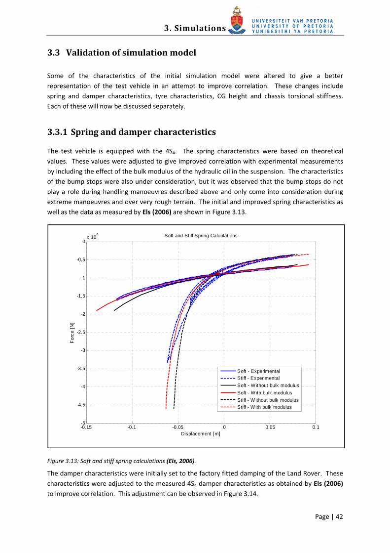
3. Simulations
Page | 42
3.3 Validation of simulation model
Some of the characteristics of the initial simulation model were altered to give a better representation of the test vehicle in an attempt to improve correlation. These changes include spring and damper characteristics, tyre characteristics, CG height and chassis torsional stiffness. Each of these will now be discussed separately.
3.3.1 Spring and damper characteristics
The test vehicle is equipped with the 4S4. The spring characteristics were based on theoretical values. These values were adjusted to give improved correlation with experimental measurements by including the effect of the bulk modulus of the hydraulic oil in the suspension. The characteristics of the bump stops were also under consideration, but it was observed that the bump stops do not play a role during handling manoeuvres described above and only come into consideration during extreme manoeuvres and over very rough terrain. The initial and improved spring characteristics as well as the data as measured by Els (2006) are shown in Figure 3.13.
Figure 3.13: Soft and stiff spring calculations (Els, 2006).
The damper characteristics were initially set to the factory fitted damping of the Land Rover. These characteristics were adjusted to the measured 4S4 damper characteristics as obtained by Els (2006) to improve correlation. This adjustment can be observed in Figure 3.14.
-0.15 -0.1 -0.05 0 0.05 0.1-5
-4.5
-4
-3.5
-3
-2.5
-2
-1.5
-1
-0.5
0x 104 Soft and Stiff Spring Calculations
Displacement [m]
Forc
e [N
]
Soft - ExperimentalStiff - ExperimentalSoft - Without bulk modulusSoft - With bulk modulusStiff - W ithout bulk modulusStiff - W ith bulk modulus

3. Simulations
Page | 43
Figure 3.14: 4S4 damper characteristics (Els, 2007).
It was also noted that the simulation model is very sensitive to these settings and should be monitored during simulations. For instance, if the mass of the vehicle is changed by more than 10%, it is highly advisable to reload the suspension accumulators and level the vehicle by means of adding or subtracting nitrogen and/or oil from the struts. This must also be done in the simulation model by changing the static force of the suspension so that the suspension struts are at 0 mm displacement if the vehicle is in static equilibrium.
3.3.2 Tyre characteristics
The characteristics of the lateral force generated by the tyre are defined by the Magic Formula in terms of the variables a0 to a13 (see paragraph 2.5.1). Two sets of values were previously used, which were generated respectively by Thoresson (2007) and Uys (2007). Later, a third set was created in between these two sets. The values of the previous and altered coefficients are given in Table 4 and the lateral force vs. slip angle for a vertical load of 10 kN is shown in Figure 3.15 for the three settings. The simulation was not very sensitive to the difference between these three settings. The difference in the results for the same simulation where the vehicle performs a DLC manoeuvre at 70 km/h with the different tyre settings are shown in Figure 3.17. Finally, it was decided that the tyre characteristics of Thoresson (2007) will be used, because these data were generated from test data where Uys (2007) modified the tyre data to obtain better correlation in the simulation.
-0.6 -0.4 -0.2 0 0.2 0.4 0.6-10
-8
-6
-4
-2
0
2
4
6
8
10
Speed (m/s)
Dam
ping
forc
e (k
N)
4S4 damper characteristics
High damping - MeasuredLow damping - MeasuredHigh damping - SimulatedLow damping - SimulatedFactory fitted damping

3. Simulations
Page | 44
It should also be mentioned that, according to MSC ADAMS (2007), the Pacejka ’89 tyre model is suitable for steady state cornering and lane change manoeuvres, but not for driving on uneven roads (Figure 3.16). The tyre model that is suitable for the most cases is FTire. Due to funding problems, we were unable to obtain a license for FTire. This makes it clear that this area needs further attention.
Table 4: Lateral stiffness coefficients used for the Pacejka ’89 tyre model.
Coefficient / reference Thoresson (2007) (Values used) Uys (2007) New coefficients a3 2125.2 9000 2380 a4 8.896 65 10
Figure 3.15: Lateral force vs. slip angle for the three Pacejka ’89 tyre models at a vertical load of 10 kN.
0 5 10 15 20 25 30 35 40 45 500
1000
2000
3000
4000
5000
6000
7000
8000
9000Pacejka '89 tire model
Slip angle (Deg)
Late
ral f
orce
(N)
Thoresson (Values used)UysNew coefficients

3. Simulations
Page | 45
Figure 3.16: Tyres suitable for different simulations conditions (MSC ADAMS, 2007).

3. Simulations
Page | 46
Figure 3.17: Results of the same simulations with the three tyre models.
3.3.3 CG height
The height of the CG point was adjusted to determine the sensitivity of this setting on the simulation. This setting had a large effect on the results, especially the roll angle of the body during a handling manoeuvre. It must also be noted that the CG height can have an error of ±10% due to the difficulty to measure this value and that this value changes when mass is added or removed from the vehicle. At the end, this value was left unchanged.
3.3.4 Chassis torsional stiffness
The chassis of the vehicle was modelled in ADAMS as two bodies connected by a torsional spring to simulate the torsional stiffness of the ladder chassis. It is crucial to model the torsional stiffness of the chassis when performing severe handling manoeuvres, so it was decided to measure this value.
To measure the torsional stiffness of the chassis, the vehicle was lifted off the ground so that all its wheels were in the air. This was done by fixing the rear bumper at two points to a mounting that is attached to the ground. One point on the front bumper was also fixed to a mounting that is attached to the ground; the other point on the front bumper was jacked up with a hydraulic jack. The force difference between the two front attachment points was measured with wheel load cells as well as the distance between the four attachment points and the floor. This information is used to calculate the angle through which the chassis twists as well as the moment that is applied to the
2 3 4 5 6 7 8
-50
0
50S
usp
disp
lace
men
t: LF
(mm
)
2 3 4 5 6 7 8
-50
0
50
Sus
p di
spla
cem
ent:
RF
(mm
)
2 3 4 5 6 7 8
-50
0
50
Sus
p di
spla
cem
ent:
LR (m
m)
2 3 4 5 6 7 8
-50
0
50
Sus
p di
spla
cem
ent:
RR
(mm
)
2 3 4 5 6 7 8
-5
0
5
Time (s)
Late
ral a
ccel
erat
ion
(m/s
2 )
2 3 4 5 6 7 8
-5
0
5
Time (s)
Ave
rage
roll
angl
e (D
eg)
Thoresson Uys New coefficients

3. Simulations
Page | 47
chassis. The chassis torsional stiffness was measured as 3040 Nm/deg where the original simulation value was 400 Nm/deg. The original simulation value was obtained through previous simulations until correlation was found. This value in the simulation model was changed to the measured value.
3.3.5 Baseline correlation
The result of the changes proposed in paragraph 3.3.1 to 3.3.4 is that the model correlates well with measured results. This can be shown by comparing measured results with the simulation results. DLC manoeuvres (as described in paragraph 2.2) were done at Gerotek Test Facilities (2008) on a long straight concrete road. A speed of 70 km/h was maintained with no anti‐roll bar (ARB) on the soft and the stiff suspension setting. Vehicle tests were regenerated with the simulations by using the measured steering angle, vehicle speed and actuator displacement (only when the ARB is passive and active) as inputs and then measuring the results. The measured data as well as the simulated results are shown in Figure 3.18 and Figure 3.19. Good correlation is found, but it is noticed that the body of the simulated vehicle moves more easily than the body of the test vehicle. This is due to friction at all the joints, connection points and seals that are not modelled in the simulation model, because the characteristics of these joints and connections points are unknown and modelled as ideal links.
The difference in suspension displacement and average roll angle between the soft and stiff suspension setting can clearly be seen by comparing Figure 3.18 and Figure 3.19.
Figure 3.18: Results of baseline vehicle and simulation during DLC manoeuvre with soft suspension.
4 6 8 10
-50
0
50
Sus
p di
spla
cem
ent:
LF (m
m)
4 6 8 10
-50
0
50
Sus
p di
spla
cem
ent:
RF
(mm
)
4 6 8 10
-50
0
50
Sus
p di
spla
cem
ent:
LR (m
m)
4 6 8 10
-50
0
50
Sus
p di
spla
cem
ent:
RR
(mm
)
4 6 8 10
-5
0
5
Late
ral a
ccel
erat
ion
(m/s
2 )
Time (s)4 6 8 10
-5
0
5
Ave
rage
roll
angl
e (D
eg)
Time (s)
MeasuredSimulated

3. Simulations
Page | 48
Figure 3.19: Results of baseline vehicle and simulation during DLC manoeuvre with stiff suspension.
3.4 Simulate proposed solution
Now that the simulation model is validated, the proposed solution can be modelled and simulated in ADAMS. The ARB was modelled by two L‐shaped arms connected by a torsion spring as shown in Figure 3.20. A torsion spring was used to model the torsional stiffness of the ARB.
The two L‐shaped arms were connected to the rear body with two revolute joints to allow rotation only in the Y‐direction. At the right hand side of the ARB (Figure 3.21), two dummy bodies with zero mass were inserted to be able to model the correct joint configuration. The end of the right L‐arm was connected to the top dummy body with a spherical joint. The two dummy bodies were then connected with a translational joint and a motion was imposed on this joint. This represented the actuator. The measured displacement of the actuator was used as input for this motion. The bottom dummy body was connected with a hooks joint to the rear axle. A hooks joint, and not a spherical joint as at the top, was used to remove the rotational degree of freedom in the Z‐direction on the two dummy bodies. In practice, two spherical joints are used and the friction at the joints restricts the rotational motion.
The left hand side of the ARB (Figure 3.22) was connected in the same way as the right hand side with the only difference being that the two dummy bodies were locked to one another. So in other words, the two dummy bodies formed a linkage. A schematic representation of how the ARB was modelled is shown in Figure 3.23.
4 6 8 10-20
-10
0
10
20
Sus
p di
spla
cem
ent:
LF (m
m)
4 6 8 10-20
-10
0
10
20
Sus
p di
spla
cem
ent:
RF
(mm
)
4 6 8 10-20
-10
0
10
20
Sus
p di
spla
cem
ent:
LR (m
m)
4 6 8 10-20
-10
0
10
20
Sus
p di
spla
cem
ent:
RR
(mm
)
4 6 8 10
-5
0
5
Late
ral a
ccel
erat
ion
(m/s
2 )
Time (s)4 6 8 10
-2
-1
0
1
2
Ave
rage
roll
angl
e (D
eg)
Time (s)
MeasuredSimulated

3. Simulations
Page | 49
Figure 3.20: Anti‐roll bar modelled in ADAMS.
Figure 3.21: Right hand side of ARB as modelled in ADAMS.
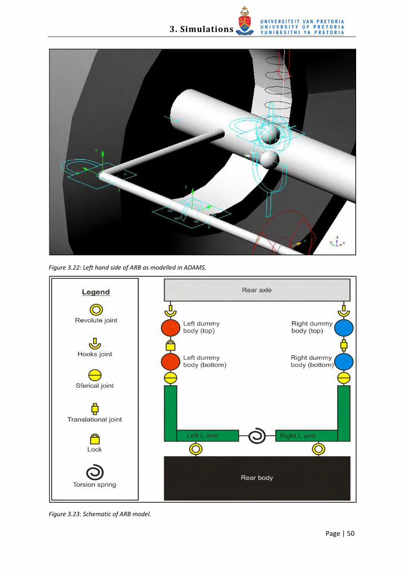
3. Simulations
Page | 50
Figure 3.22: Left hand side of ARB as modelled in ADAMS.
Figure 3.23: Schematic of ARB model.

3. Simulations
Page | 51
In order to simulate the proposed solution, a function was written in Matlab, which calculates the desired displacement of the AARB actuator. This was done by filtering the simulated lateral acceleration with a Bessel low pass filter (8th order, 6Hz cut off frequency) and then limiting this value to an absolute maximum of 0.4 g. The limiter was implemented so that the AARB (Active anti‐roll bar) system reduces the body roll angle to zero up to a lateral acceleration of 0.4 g and from there the body roll per lateral acceleration increases at the same rate as with the passive ARB. This was done to start warning the driver that the linearity limit of the vehicle is exceeded. 0.4 g was chosen because it is about half of the lateral acceleration the vehicle can generate, so it is a safe limit and all the related solutions found in the literature were limited between 0.35 g and 0.5 g lateral acceleration.
Then the filtered lateral acceleration was multiplied by a gain (26 mm/m.s‐2) to convert it to actuator displacement. The gain was obtained through trial and error with the simulations. Finally, a velocity limiter was built in with a value of 0.3 m/s to enable a limitation of the maximum velocity of the actuator. This was done to determine the maximum speed needed for the system to operate properly. The desired actuator displacement was then sent back to ADAMS to be used in the simulation. All of these calculations were done simultaneously with the simulations.
The simulations were done and the system was optimised until the best results were obtained. These results are shown in Figure 3.24 and Figure 3.25. Figure 3.24 shows an 80% improvement in body roll angle on a concrete road during a DLC manoeuvre at 70 km/h. Figure 3.25 indicates a 41% improvement on Belgian paving during a DLC manoeuvre at 50 km/h.
Figure 3.24: Average body roll angle of the test vehicle during a DLC manoeuvre at 70km/h on a concrete road.
0 1 2 3 4 5 6 7 8 9 10-6
-4
-2
0
2
4
6
Time (s)
Ave
rage
bod
y ro
ll an
gle
(Deg
)
Body roll angle: Base vehicle vs AARB vehicle on flat road
Base vehicleAARB vehicle

3. Simulations
Page | 52
Figure 3.25: Average body roll angle of the test vehicle during a DLC manoeuvre at 50km/h on Belgian paving.
The following design specifications were obtained from the initial simulations: torque in the ARB, ARB torsional stiffness, ARB arm length, actuator maximum speed, actuator displacement, controller filters, controller gains and controller dependant sensors.
The values obtained from the initial simulations are shown in Table 5. These values were altered with the ability of the hardware in mind, to avoid unrealistic values being chosen.
Table 5: Design parameters obtained from simulations:
Design parameter: Design value: Maximum torque in the ARB 1000 Nm ARB torsional stiffness 85 Nm/deg ARB arm length 0.45 m Actuator maximum speed 0.3 m/s Actuator displacement 200 mm Controller filters Bessel low pass filter (8th order, 6 Hz cut off frequency) Controller gains 26 mm/m.s‐2 (Actuator displacement per lateral acceleration) Controller dependant sensors Lateral acceleration
Some of the design parameters will now be discussed to give insight into the decision‐making process. First, the actuator displacement was chosen according to the space envelope available on the test vehicle. Simulations were also done using the speed of the vehicle and the steering angle as dependant sensors, but the lateral acceleration produced the best results. Then the ARB torsional
0 2 4 6 8 10 12 14-4
-3
-2
-1
0
1
2
3
4Body roll angle: Base vehicle vs AARB vehicle on rough road
Time (s)
Ave
rage
bod
y ro
ll an
gle
(Deg
)Base vehicleAARB vehicle
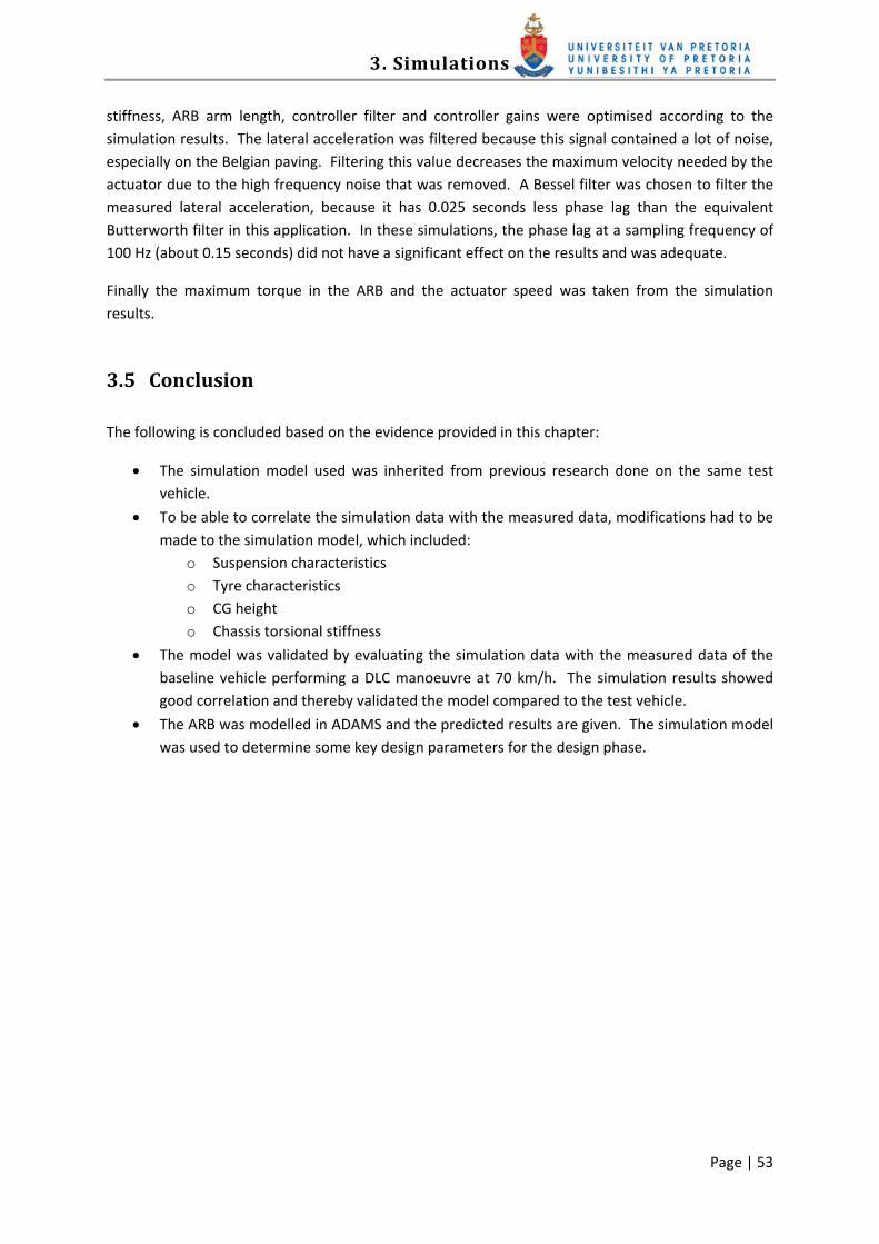
3. Simulations
Page | 53
stiffness, ARB arm length, controller filter and controller gains were optimised according to the simulation results. The lateral acceleration was filtered because this signal contained a lot of noise, especially on the Belgian paving. Filtering this value decreases the maximum velocity needed by the actuator due to the high frequency noise that was removed. A Bessel filter was chosen to filter the measured lateral acceleration, because it has 0.025 seconds less phase lag than the equivalent Butterworth filter in this application. In these simulations, the phase lag at a sampling frequency of 100 Hz (about 0.15 seconds) did not have a significant effect on the results and was adequate.
Finally the maximum torque in the ARB and the actuator speed was taken from the simulation results.
3.5 Conclusion
The following is concluded based on the evidence provided in this chapter:
• The simulation model used was inherited from previous research done on the same test vehicle.
• To be able to correlate the simulation data with the measured data, modifications had to be made to the simulation model, which included:
o Suspension characteristics o Tyre characteristics o CG height o Chassis torsional stiffness
• The model was validated by evaluating the simulation data with the measured data of the baseline vehicle performing a DLC manoeuvre at 70 km/h. The simulation results showed good correlation and thereby validated the model compared to the test vehicle.
• The ARB was modelled in ADAMS and the predicted results are given. The simulation model was used to determine some key design parameters for the design phase.

Page | 54
4 Active antiroll bar design, development and testing
In this chapter the design process together with some key design calculations are discussed. This is followed by laboratory testing, characterisation and implementation on the test vehicle. Finally the sensors and measuring equipment are discussed.
4.1 Design and manufacturing
Due to the small space envelope available at the front of the test vehicle, it was decided to implement an AARB system only on the rear of the vehicle.
A computer aided design (CAD) model of the AARB system was built in Solid Works (Figure 4.1). This was done to minimise design error, obtain 2D drawings of all the components that had to be manufactured and to perform a space envelope analysis on the system.
Figure 4.1: CAD of AARB system.
The design requirements as obtained from the simulations were used to calculate the specifications of the system and will now be discussed.
From the CAD model, the effective length ( )L of the shaft of the ARB is given as 1.078 m. The shear
modulus of elasticity ( )G of steel is given as 80 GPa (Gere, 2004). If the diameter of the shaft
( )2d r= is taken as 29 mm, the torsional stiffness ( )tk of the ARB shaft can be calculated as follows
(Gere, 2004):
4. Active antiroll bar design, development and testing
Page | 55
( )( )
( ) ( )( )
4
49
/ 2
80 10 0.0145 / 2
1.0785153 /89.9 /
pt
t
t
t
t
GIk
LG r
kL
k
k Nm radk Nm
π
π
=
=
×=
=
= °
Where:
4 / 2pI rπ= =Polar moment of inertia (m4)
r = Radius of the shaft (m)
This value of 89.9 Nm/° is close enough to the design parameter obtained from the simulations of 85 Nm/°, keeping in mind that the elasticity of the other components of the ARB will reduce this value. Therefore it was decided to manufacture the ARB with a 29 mm diameter shaft. The shaft must be
able to withstand 1000 Nm torque ( )T together with a reasonable safety factor. The maximum
shear stress ( )maxτ in the shaft with a 1000 Nm torque applied to it in the axial direction can be
calculated by (Gere, 2004):
( )( )( )
max
max 4
max 4
max
/ 21000 0.0145
0145 / 2208.8
p
TrI
Trr
MPa
τ
τπ
τπ
τ
=
=
=
=
Due to this high predicted shear stress value, it was decided to use EN24 steel for the shaft of the ARB. The yield strength of this steel is given as 635 MPa minimum (Midrand special steels, 2008), which gives a safety factor of 3.04. This is acceptable for this application.
The fatigue limit for steel can be estimated as 0.5 uσ , where uσ is the ultimate tensile strength of
the steel. (Gere, 2004) For EN24 steel, the minimum ultimate tensile strength is given as
850u MPaσ = (Midrand special steels, 2008), which gives an estimated fatigue limit of 425MPa .
This fatigue limit is larger than the maximum calculated stress in the shaft ( )208.8MPa . This
shows that the shaft of the ARB will never fail due to fatigue and that this component has a fatigue safety factor of 2.04.

4. Active antiroll bar design, development and testing
Page | 56
The arm length is specified as 0.45m from which the force ( )F on the hydraulic cylinder can be
calculated by:
( ) ( )/
1000 / 0.452222
F T LFF N
=
=
=
If the outer and inner diameters of the cylinder are chosen 40 and 30 mm, the area ( )A where the
hydraulic pressure acts is calculated as 45.5 10A m−= × . Now the required pressure ( )P can be
calculated by:
( ) ( )4
/
2222 / 5.5 10
4.04
P F A
P
P MPa
−
=
= ×
=
A pressure of 8 MPa was chosen to overcome the flow losses, friction in the system and be able to maintain pressure during pressure drops due to high flow rates. The hydraulic pump that will be used can deliver up to 20 MPa pressure (Stone Hydraulics, 2008).
The hydraulic cylinder was also manufactured. The CAD (computer aided design) model is shown in Figure 4.2 and the manufactured cylinder is shown in Figure 4.3.
Figure 4.2: CAD view of the hydraulic cylinder design.

4. Active antiroll bar design, development and testing
Page | 57
Figure 4.3: The manufactured hydraulic cylinder.
The sealing setup used was the standard setup from Trelleborg Sealing Solutions (2007). The cylinder was mounted between two spherical joints to minimise the moments exerted on the cylinder. As the plan was to use the existing hydraulic pump used for ride height adjustment on the 4S4, the same hydraulic fluid namely Aeroshell Fluid 41 was used in this hydraulic system. The flow was controlled by a MOOG hydraulic servo valve (Figure 4.4) with a maximum flow rate of 19 l/min. Displacement feedback was used to control the position of the cylinder which was done with a string displacement meter. A Zwick Roell K7500 servo controller was used to control the servo valve. It was decided to add a valve between the top and the bottom of the cylinder, which connects the two sides so that the cylinder can be moved with minimal force when the valve is open (Figure 4.4). So when the ARB needs to be disconnected, the valve is opened and when the ARB is connected, the valve is closed.
Figure 4.4: MOOG hydraulic servo valve used to control the hydraulic cylinder and the bypass valve.

4. Active antiroll bar design, development and testing
Page | 58
The hydraulic pump is a Stone hydraulic power pack (Figure 4.5). This power pack was initially used to level the vehicle when the 4S4 suspension struts where reloaded with gas and to increase or decrease the ride height of the vehicle for vehicle tests. This system consists of a 12V DC electric motor, a hydraulic pump and a reservoir. The electric motor has a maximum rotational speed of 3000 RPM and the existing hydraulic pump delivers 1cc per revolution. This gives a maximum flow rate of 3 l/min. This had to be increased, as a maximum flow rate of 10.1 l/min is needed for the cylinder to reach a maximum speed of 0.3 m/s. For this reason a 4 cc per revolution hydraulic pump was fitted to give a maximum flow rate of 12 l/min. The reservoir can store 5.6 l, which is sufficient for this application (Stone Hydraulics, 2008).
Figure 4.5: Stone hydraulic power pack.
4.2 Bench testing
After the ARB was manufactured a test setup was built in the laboratory to measure the torsional stiffness of the ARB and to calibrate the strain gauge used to measure the torque in the ARB. The manufactured ARB is shown in Figure 4.6 and the test setup in Figure 4.7.

4. Active antiroll bar design, development and testing
Page | 59
Figure 4.6: The manufactured ARB.
Figure 4.7: ARB test bench setup.

4. Active antiroll bar design, development and testing
Page | 60
For the test setup, the two brackets that bolt to the chassis of the test vehicle and keep the ARB in place was removed from the vehicle and clamped to a stable platform. The one arm was also stabilised on the same platform. On the other arm, weights were added to impose torsion on the shaft of the ARB. A fixed point on the stable platform was used as reference point to measure the deflection of the arm. The torsional stiffness of the ARB was measured by calculating the torque imposed on the shaft of the ARB by means of the weight added. The angle through which the ARB rotated was calculated from the deflection of the end of the arm on which the weights were added. The measured results for the loading and unloading of the ARB are shown in Figure 4.8. The offset between the loading and unloading measurements are due to friction at the joints and connection points. This phenomenon shown in Figure 4.8 is called a hysteresis loop.
Figure 4.8: Measured torsional stiffness of ARB.
The inverse of the average slope of these measured results is 81.5 Nm/deg. The difference between the measured and the calculated stiffness is due to the deflection of the arms and joints. This also shows that the deflection of the arms and joints contributes 9.3% to torsional stiffness of the whole ARB.
The same test bench was used to calibrate the strain gauge. Two 0°‐90° strain gauges were used, placed at the top and the bottom of the shaft of the ARB at an angle of 45° (Figure 4.9). These strain gauges were connected in a full bridge configuration to measure the torque in the ARB. The strain gauge was calibrated by imposing a known torque on the ARB and tuning the controller to take the
0 50 100 150 200 250 3000
0.5
1
1.5
2
2.5
3
3.5
4ARB torsional stiffness
Torque (Nm)
Ang
le o
f rot
atio
n (D
eg)
Loading
Unloading
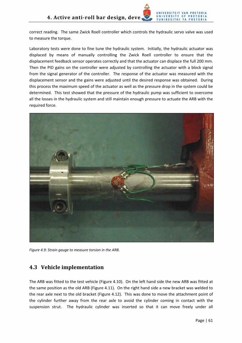
4. Active antiroll bar design, development and testing
Page | 61
correct reading. The same Zwick Roell controller which controls the hydraulic servo valve was used to measure the torque.
Laboratory tests were done to fine tune the hydraulic system. Initially, the hydraulic actuator was displaced by means of manually controlling the Zwick Roell controller to ensure that the displacement feedback sensor operates correctly and that the actuator can displace the full 200 mm. Then the PID gains on the controller were adjusted by controlling the actuator with a block signal from the signal generator of the controller. The response of the actuator was measured with the displacement sensor and the gains were adjusted until the desired response was obtained. During this process the maximum speed of the actuator as well as the pressure drop in the system could be determined. This test showed that the pressure of the hydraulic pump was sufficient to overcome all the losses in the hydraulic system and still maintain enough pressure to actuate the ARB with the required force.
Figure 4.9: Strain gauge to measure torsion in the ARB.
4.3 Vehicle implementation
The ARB was fitted to the test vehicle (Figure 4.10). On the left hand side the new ARB was fitted at the same position as the old ARB (Figure 4.11). On the right hand side a new bracket was welded to the rear axle next to the old bracket (Figure 4.12). This was done to move the attachment point of the cylinder further away from the rear axle to avoid the cylinder coming in contact with the suspension strut. The hydraulic cylinder was inserted so that it can move freely under all

4. Active antiroll bar design, development and testing
Page | 62
circumstances. The cylinder was connected to the hydraulic power pack and the MOOG valve to the servo controller.
The vehicle was fitted with a PC 104 form factor data acquisition computer (Figure 4.13) running Turbo Pascal in DOS that can read and record 16 analogue channels and 8 digital channels. It can also provide 4 analogue output channels and 8 digital output channels. This computer was used to record all the measured data, switch the hydraulic pump and the hydraulic relief valve and compute the desired cylinder displacement. All the channels that were measured are shown in Table 6. The Bessel filter used in the signal‐processing phase to calculate the desired cylinder displacement was programmed in Turbo Pascal on the PC 104 form factor computer so that it can be easily altered if needed.
Figure 4.10: AARB fitted to the test vehicle.
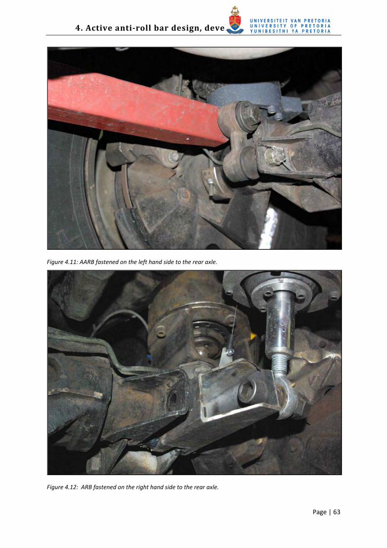
4. Active antiroll bar design, development and testing
Page | 63
Figure 4.11: AARB fastened on the left hand side to the rear axle.
Figure 4.12: ARB fastened on the right hand side to the rear axle.
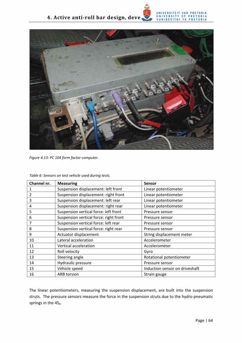
4. Active antiroll bar design, development and testing
Page | 64
Figure 4.13: PC 104 form factor computer.
Table 6: Sensors on test vehicle used during tests.
Channel nr. Measuring Sensor 1 Suspension displacement: left front Linear potentiometer 2 Suspension displacement: right front Linear potentiometer 3 Suspension displacement: left rear Linear potentiometer 4 Suspension displacement: right rear Linear potentiometer 5 Suspension vertical force: left front Pressure sensor 6 Suspension vertical force: right front Pressure sensor 7 Suspension vertical force: left rear Pressure sensor 8 Suspension vertical force: right rear Pressure sensor 9 Actuator displacement String displacement meter 10 Lateral acceleration Accelerometer 11 Vertical acceleration Accelerometer 12 Roll velocity Gyro 13 Steering angle Rotational potentiometer 14 Hydraulic pressure Pressure sensor 15 Vehicle speed Induction sensor on driveshaft 16 ARB torsion Strain gauge
The linear potentiometers, measuring the suspension displacement, are built into the suspension struts. The pressure sensors measure the force in the suspension struts due to the hydro pneumatic springs in the 4S4.

4. Active antiroll bar design, development and testing
Page | 65
Originally, a tilt sensor was used to measure the body roll angle of the vehicle, but it was found that these readings were suspiciously high. This was due to the fact that the tilt sensor takes the vertical and lateral acceleration into consideration during handling manoeuvres. This sensor has a built‐in low pass filter and can filter out higher frequencies, but very low frequencies (as experienced during a lane change handling manoeuvre) is measured as a change in tilt angle. The data from the gyro, measuring the roll velocity, was integrated to give roll angle but the drift on this data had such a big influence that it could not be used to measure body roll angle. Body roll was therefore calculated from the left and the right suspension displacements. These calculations do not include tyre deflections, but an accurate and reliable measurement could be made.
The lateral and vertical accelerations were measured by a tri‐axial accelerometer positioned near the CG point on the body of the vehicle. The steering angle was measured with a rotational potentiometer on the kingpin of the right front wheel.
Two Deltec 12 V, 105 Ah deep cycle batteries were fitted to the vehicle and connected in parallel to supply the hydraulic power pack and the measuring instrumentation. This auxiliary battery pack was charged with an external charger when testing in the laboratory and the engine of the vehicle was not running. During the test sessions at Gerotek the alternator of the engine was used to charge the auxiliary battery pack. This was done by inserting an auxiliary battery unit between the vehicle battery and the auxiliary battery pack. This unit charges the auxiliary battery pack when its voltage is lower than the voltage of the vehicle battery and disconnects the auxiliary battery when it is fully charged. This significantly increased the amount of tests that could be done during a test session.
4.4 Conclusion
The following is concluded based on the evidence provided in this chapter:
• All the hardware was designed in Solid Works according to the design parameters obtained from the simulations.
• The components were manufactured and assembled.
• The torsional stiffness of the ARB was measured to verify the design specification.
• The system was implemented on the vehicle and the necessary sensors were fitted to the vehicle to measure the response of the vehicle. The control system was programmed onto the PC 104 form factor computer, which also stored the measured data.
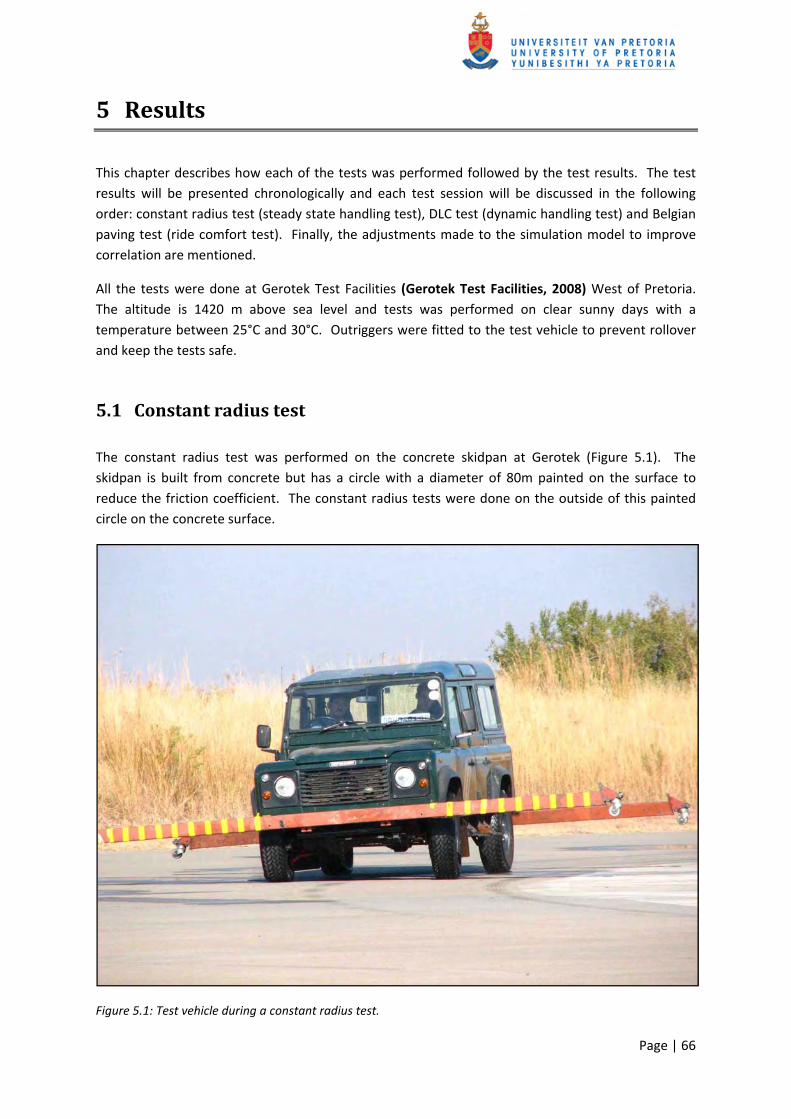
Page | 66
5 Results
This chapter describes how each of the tests was performed followed by the test results. The test results will be presented chronologically and each test session will be discussed in the following order: constant radius test (steady state handling test), DLC test (dynamic handling test) and Belgian paving test (ride comfort test). Finally, the adjustments made to the simulation model to improve correlation are mentioned.
All the tests were done at Gerotek Test Facilities (Gerotek Test Facilities, 2008) West of Pretoria. The altitude is 1420 m above sea level and tests was performed on clear sunny days with a temperature between 25°C and 30°C. Outriggers were fitted to the test vehicle to prevent rollover and keep the tests safe.
5.1 Constant radius test
The constant radius test was performed on the concrete skidpan at Gerotek (Figure 5.1). The skidpan is built from concrete but has a circle with a diameter of 80m painted on the surface to reduce the friction coefficient. The constant radius tests were done on the outside of this painted circle on the concrete surface.
Figure 5.1: Test vehicle during a constant radius test.

5. Results
Page | 67
All the tests were done by slowly accelerating the vehicle from standstill, maintaining the radius until the outrigger hits the ground (due to the large body roll angle) or it becomes impossible to maintain the constant radius due to the vehicle sliding out. Six runs were done as shown in Table 7. The soft suspension setting refers to soft spring and low damping while the stiff suspension setting refers to stiff spring and high damping.
During initial tests, the ARB was “disconnected” by opening the bypass valve. Results indicated that flow losses still had a significant effect on the vehicle due to the ARB. The ARB was subsequently disconnected mechanically. For the passive ARB setting, the actuator was “locked” initially by closing all the hydraulic valves. Again, fluid compressibility and the MOOG valve not closing properly caused the actuator to move. The actuator was subsequently controlled actively with the hydraulic system to remain in the static position to make sure that it does not move during the tests.
Table 7: Constant radius test runs done.
Test no. ARB setting 4S4 suspension setting 1 Disconnected Soft 2 Disconnected Stiff 3 Passive Soft 4 Passive Stiff 5 Active Soft 6 Active Stiff
5.2 Doublelanechangetest
The DLC test was performed as described in paragraph 2.2. It was decided to do this test at a speed of 70 km/h because it is about the limit where this test can safely be performed with all the suspension settings. The speed of the vehicle was kept as constant as possible by the driver and the same driver was used for all tests. A sequence of photos of a DLC manoeuvre is shown in Figure 5.2. The same configurations were used as for the constant radius test (Table 7).
5.3 Belgian paving test
Three runs were performed on the Belgian paving as shown in Table 8. No tests were performed on the stiff suspension setting because the ride is highly uncomfortable. The speed was kept constant by driving in first gear against the governor of the diesel engine. This ensured a constant speed throughout the test as well as a repeatable speed during all the runs. Figure 5.3 shows the test vehicle on the Belgian paving.
Table 8: Belgian paving test runs done.
Test no. ARB setting Suspension setting 1 Disconnected Soft 2 Passive Soft 3 Active Soft

5. Results
Page | 68
Figure 5.2: DLC manoeuvre sequence.
Figure 5.3: Belgian paving test run.

5. Results
Page | 69
Three test sessions were performed and will now be discussed where only the relevant information will be presented.
5.4 Test session 1
Constant radius tests, DLC tests and Belgian paving tests were performed in this test session.
5.4.1 Constant radius test
Only two test runs were performed on the soft suspension setting, with the ARB disconnected and the passive ARB. This was due the battery pack that was depleted at this point of the test session and at this stage it did not seem necessary to do constant radius tests on the stiff suspension setting. Later the need for it became clear to obtain a set of reference measurements.
Figure 5.4 shows the average of the front and the rear body roll angles, calculated from the suspension displacements, vs. the lateral acceleration for the two test runs done. This shows the reduction in roll angle due to the connection of the ARB. This proves that connecting the ARB decreases the maximum body roll angle by 56% during a steady state handling test compared to the vehicle without an ARB.
Figure 5.4: Constant radius test: average body roll angle vs. lateral acceleration.
-1 0 1 2 3 4 5 6 7-1
0
1
2
3
4
5
6
7
8
Lateral acceleration (m/s2)
Ave
rage
bod
y ro
ll an
gle
(Deg
)
Soft suspension, ARB disconnectedSoft suspension, ARB connected
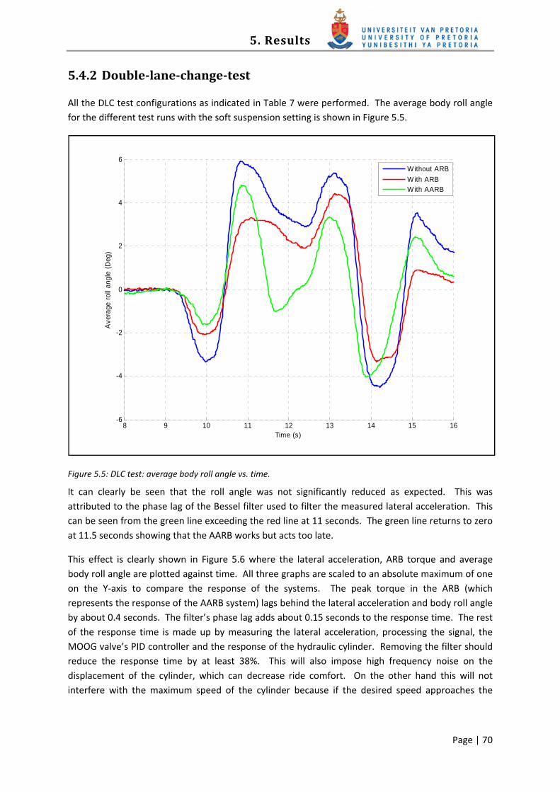
5. Results
Page | 70
5.4.2 Doublelanechangetest
All the DLC test configurations as indicated in Table 7 were performed. The average body roll angle for the different test runs with the soft suspension setting is shown in Figure 5.5.
Figure 5.5: DLC test: average body roll angle vs. time.
It can clearly be seen that the roll angle was not significantly reduced as expected. This was attributed to the phase lag of the Bessel filter used to filter the measured lateral acceleration. This can be seen from the green line exceeding the red line at 11 seconds. The green line returns to zero at 11.5 seconds showing that the AARB works but acts too late.
This effect is clearly shown in Figure 5.6 where the lateral acceleration, ARB torque and average body roll angle are plotted against time. All three graphs are scaled to an absolute maximum of one on the Y‐axis to compare the response of the systems. The peak torque in the ARB (which represents the response of the AARB system) lags behind the lateral acceleration and body roll angle by about 0.4 seconds. The filter’s phase lag adds about 0.15 seconds to the response time. The rest of the response time is made up by measuring the lateral acceleration, processing the signal, the MOOG valve’s PID controller and the response of the hydraulic cylinder. Removing the filter should reduce the response time by at least 38%. This will also impose high frequency noise on the displacement of the cylinder, which can decrease ride comfort. On the other hand this will not interfere with the maximum speed of the cylinder because if the desired speed approaches the
8 9 10 11 12 13 14 15 16-6
-4
-2
0
2
4
6
Time (s)
Ave
rage
roll
angl
e (D
eg)
W ithout ARBWith ARBWith AARB
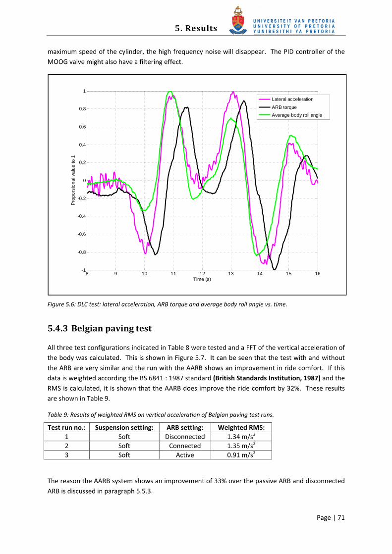
5. Results
Page | 71
maximum speed of the cylinder, the high frequency noise will disappear. The PID controller of the MOOG valve might also have a filtering effect.
Figure 5.6: DLC test: lateral acceleration, ARB torque and average body roll angle vs. time.
5.4.3 Belgian paving test
All three test configurations indicated in Table 8 were tested and a FFT of the vertical acceleration of the body was calculated. This is shown in Figure 5.7. It can be seen that the test with and without the ARB are very similar and the run with the AARB shows an improvement in ride comfort. If this data is weighted according the BS 6841 : 1987 standard (British Standards Institution, 1987) and the RMS is calculated, it is shown that the AARB does improve the ride comfort by 32%. These results are shown in Table 9.
Table 9: Results of weighted RMS on vertical acceleration of Belgian paving test runs.
Test run no.: Suspension setting: ARB setting: Weighted RMS: 1 Soft Disconnected 1.34 m/s2 2 Soft Connected 1.35 m/s2 3 Soft Active 0.91 m/s2
The reason the AARB system shows an improvement of 33% over the passive ARB and disconnected ARB is discussed in paragraph 5.5.3.
8 9 10 11 12 13 14 15 16-1
-0.8
-0.6
-0.4
-0.2
0
0.2
0.4
0.6
0.8
1
Time (s)
Pro
pors
iona
l val
ue to
1
Lateral acceleration
ARB torqueAverage body roll angle

5. Results
Page | 72
Figure 5.7: Belgian paving test: FFT of vertical acceleration.
From test session 1, it is concluded that the AARB system can improve the handling of the vehicle, but the response time of the system has to be improved by reducing the lag in the system before the expected result can be obtained.
5.4.4 Adjustments after test session 1
Laboratory tests were done where the lateral acceleration, measured on the vehicle during test session 1 was used as input and the response of the hydraulic cylinder was measured. Figure 5.8 shows the response of the cylinder with and without the Bessel filter. The increased higher frequency content is clearly visible but the lag is decreased by as much as 0.5 seconds. The cylinder cannot keep up with the high frequencies. The cylinder’s controller, MOOG valve and cylinder response acts as a low‐pass filter.
As two alternatives, a 5‐point running average and 10‐point running average filter were also implemented as two alternatives. The response of these filters is shown in Figure 5.9. From this, it seems as if the 5‐point running average or 10‐point running average filter will give the best results, depending on the amount of lag that can be tolerated and if the higher frequencies decreases the ride comfort. The filters reduce the noise but result in phase lag added to the system. A test was done on campus by driving around a corner on a tar road at 40 km/h and measuring the vertical acceleration to see if the different filters affect the ride comfort of the vehicle. All the runs were
0 5 10 15 20 25 30 35 40 45 500
0.1
0.2
0.3
0.4
0.5
0.6
0.7
0.8
0.9
1
Frequency (Hz)
Mag
nitu
de o
f ver
tical
acc
eler
atio
n (m
/s2 )W ithout ARBWith ARBWith AARB

5. Results
Page | 73
done with soft suspension and the AARB. The results of the weighted RMS of the vertical acceleration are given in Table 10.
Table 10: Weighted RMS on vertical acceleration with different filters.
Filter Weighted RMS No filter 0.46 m/s2 5‐point mean running average 0.42 m/s2 10‐point mean running average 0.38 m/s2 Bessel filter 0.39 m/s2
Figure 5.8: Response of cylinder with and without the Bessel filter.
From Table 10, it is clear that the different filters have an effect on the ride comfort but this effect is so small that it can be neglected. So it was decided that no filter will be used in test session 2.
Another change made was that the resistance was minimised between the vehicle battery and the auxiliary battery by removing a safety resistance in the circuit installed by the company who installed the auxiliary battery unit. This was done so that the alternator of the vehicle charges the auxiliary battery more efficiently.
6 7 8 9 10 11 12 13 14 15 16
-100
-50
0
50
100
Time (s)
Act
uato
r dis
plac
emen
t (m
)
Regenerated test with no filterMeasured during test with Bessel filter

5. Results
Page | 74
Figure 5.9: Effect of different filters on lateral acceleration.
5.5 Test session 2
Constant radius tests, DLC tests and Belgian paving tests were performed in this test session.
5.5.1 Constant radius test
This time, six configurations were tested as indicated in Table 7. The average body roll angle vs. lateral acceleration for the three runs with the soft suspension setting are shown in Figure 5.10.
The two runs with the ARB disconnected and ARB connected is identical. It is probably due to the MOOG valve being open for some reason and the hydraulic fluid flowing freely from one side to the other of the hydraulic cylinder, independent of the setting of the bypass valve. The second thing that is noticed is that the AARB is not effective enough. It should show zero body roll up to 0.4 g with the AARB and from there increase at the same rate as with the connected ARB.
Figure 5.11 shows the same graph for the stiff suspension setting. The same two problems can be observed in this graph.
13.6 13.7 13.8 13.9 14 14.1 14.2 14.3 14.4
2.6
2.8
3
3.2
3.4
3.6
3.8
Time (s)
Late
ral a
ccel
erat
ion
(m/s
2 )Lateral accelerationBessel filter5-point mean running average10-point mean running average

5. Results
Page | 75
Figure 5.10: Constant radius test: average body roll angle vs. lateral acceleration with soft suspension.
Figure 5.11: Constant radius test: average body roll angle vs. lateral acceleration with stiff suspension.
-1 0 1 2 3 4 5 6 7-1
0
1
2
3
4
5
6
7
8
Lateral acceleration (m/s2)
Ave
rage
bod
y ro
ll an
gle
(Deg
)
Soft suspension, ARB disconnectedSoft suspension, ARB connectedSoft suspension, AARB
-1 0 1 2 3 4 5 6 7 8-0.5
0
0.5
1
1.5
2
2.5
3
3.5
4
Lateral acceleration (m/s2)
Ave
rage
bod
y ro
ll an
gle
(Deg
)
Stiff suspension, ARB disconnectedStiff suspension, ARB connectedStiff suspension, AARB

5. Results
Page | 76
5.5.2 Doublelanechangetest
All six configurations were tested in this test session. First, the average body roll angle vs. time of the three runs for the soft suspension (Figure 5.12) and the stiff suspension (Figure 5.13) were analysed.
Figure 5.12: DLC test: average body roll angle vs. time with soft suspension.
From these graphs, it seems that the response time of the system is within an acceptable range. The AARB system decreases the maximum roll angle by 18% for the soft suspension and 36% for the stiff suspension. This is an improvement but not as great as predicted by the simulations. This verifies the assumption made from the constant radius test that the effect of the AARB system has to be increased.
The system response for the run with the soft suspension and the AARB is shown in Figure 5.14. From this graph it is clear that the response time of the AARB system is not problematic any more and that it reacts immediately.
6 7 8 9 10 11 12 13 14-4
-3
-2
-1
0
1
2
3
4
Time (s)
Ave
rage
roll
angl
e (D
eg)
W ithout ARBWith ARBWith AARB

5. Results
Page | 77
Figure 5.13: DLC test: average body roll angle vs. time with stiff suspension.
Figure 5.14: DLC test: lateral acceleration, ARB torque and average body roll angle vs. time.
6 7 8 9 10 11 12 13 14
-1
-0.8
-0.6
-0.4
-0.2
0
0.2
0.4
0.6
0.8
1
Time (s)
Ave
rage
roll
angl
e (D
eg)
W ithout ARBWith ARBWith AARB
6 7 8 9 10 11 12 13 14-1
-0.8
-0.6
-0.4
-0.2
0
0.2
0.4
0.6
0.8
1
Time (s)
Pro
pors
iona
l val
ue to
1
Lateral accelerationARB torqueAverage body roll angle

5. Results
Page | 78
5.5.3 Belgian paving test
All three configurations were tested in this test session on the Belgian paving. The values of the weighted RMS vertical acceleration are given in Table 11 and the FFT of the vertical acceleration of the vehicle body is shown in Figure 5.15.
Table 11: Results of weighted RMS on vertical acceleration for Belgian paving test runs.
Test run no.: Suspension setting: ARB setting: Weighted RMS: 1 Soft Disconnected 1.43 m/s2 2 Soft Connected 1.41 m/s2 3 Soft Active 1.44 m/s2
Figure 5.15: Belgian paving test: FFT of vertical acceleration.
In this case all three test runs gave almost identical ride comfort results. From this, it can be concluded that the AARB system without a filter has no detrimental effect on the ride comfort of the vehicle.
This also concludes that the Bessel filter that was in the system improved the ride comfort by 33% over the passive ARB and disconnected ARB systems as shown in Table 9. This is probably due to the lag added to the system by the filter, which made the AARB system act as a damper on the body roll of the vehicle. While the AARB system with no filter only increases the roll stiffness on the vehicle. This is definitely an area of possible future work to be investigated.
0 5 10 15 20 25 30 35 40 45 500
0.1
0.2
0.3
0.4
0.5
0.6
0.7
0.8FFT of vertical acceleration
Frequency (Hz)
Mag
nitu
de o
f ver
tical
acc
eler
atio
n (m
/s2 )
W ith ARB disconnectedWith ARB connectedWith AARB

5. Results
Page | 79
The reason why the weighted RMS values in test session 2 (Table 11) are 8% higher than the weighted RMS values from test session 1 (Table 9) is due to the fact that the speed at which the tests were done on the two days are not the same. During test session 1, all the test runs were done at 41 km/h and during test session 2, all the test runs were done at 38 km/h. The exact reason why the speed is slightly different is unknown, but it has to do with the maximum revolutions of the engine where the governor limits the engine.
From test session 2, it is concluded that the gain of the AARB system is too low and that the bypass valve on the cylinder does not have the desired effect on the system. It is also found that the AARB system has no significant effect on the ride comfort of the system if the lag in the system is kept to a minimum.
5.5.4 Adjustments after test session 2
The gain with which the measured lateral acceleration is multiplied to get the desired actuator displacement was additionally multiplied with 1.2 to increase the effect of the AARB system. This multiplication factor was determined experimentally.
The other change made was to perform two runs directly after each other for each configuration. This was done to give the driver a feel of how the vehicle reacts during a specific manoeuvre, because the response of the vehicle changes quite significantly between the different settings, thus the driver’s input must also change. The steering input of the driver for three different ARB settings for the soft suspension setting is shown in Figure 5.16.
Figure 5.16: Steering angles during three DLC manoeuvres with soft suspension.
3 4 5 6 7 8 9 10 11-4
-3
-2
-1
0
1
2
3
4
Time (s)
Ste
erin
g an
gle
(Deg
)
W ithout ARBWith ARBWith AARB

5. Results
Page | 80
The third change implemented for test session 3 was that the ARB was manually bolted loose from the axle when the ARB was disconnected. For passive ARB tests, the actuator was kept at its corresponding position for zero lateral acceleration by the hydraulic system. This was done by manually setting the measured lateral accelerations to zero in the program on the PC 104 form factor computer. This way, the setting of the MOOG valve or the bypass valve has no unknown effect on the test results.
5.6 Test session 3
Only constant radius tests and DLC tests were done during this test session.
5.6.1 Constant radius test
All the configurations were tested two times. The body roll angle vs. lateral acceleration for the three settings with the soft suspension are shown in Figure 5.17 and with the stiff suspension in Figure 5.18. These results show exactly what is expected from the system. The case with the disconnected ARB shows the most body roll. The case with the connected ARB shows significantly less body roll and the case with the AARB shows zero body roll up to about 0.4 g. Above 0.4 g, body roll increases at the same rate as the connected ARB.
Figure 5.17: Constant radius test: average body roll angle vs. lateral acceleration with soft suspension.
-1 0 1 2 3 4 5 6 7 8-1
0
1
2
3
4
5
6
7
Lateral acceleration (m/s2)
Ave
rage
bod
y ro
ll an
gle
(Deg
)
Soft suspension, ARB disconnectedSoft suspension, ARB connectedSoft suspension, AARB

5. Results
Page | 81
Figure 5.18: Constant radius test: average body roll angle vs. lateral acceleration with stiff suspension.
5.6.2 Doublelanechangetest
Twelve runs were performed in this test session with six configurations. First, the average body roll angle vs. time of the three runs for the soft suspension (Figure 5.19) and the stiff suspension (Figure 5.20) were investigated. For the soft suspension, there is an improvement in average body roll angle between the disconnected ARB and the AARB of 74% and for the stiff suspension an improvement of 45%. This is a substantial improvement and very close to the 80% improvement predicted by the simulations for the soft suspension. For the soft suspension setting, the AARB shows a 55% improvement in body roll over the passive ARB and an improvement of 40% with the stiff suspension setting.
From test session 3 it is concluded that the AARB system responds as expected by reducing the body roll angle to zero up to 0.4 g lateral acceleration. An improvement of 74% is found in the body roll angle of the vehicle during a DLC manoeuvre at 70 km/h compared to the test run with the soft suspension setting and the ARB disconnected.
-1 0 1 2 3 4 5 6 7 8-0.5
0
0.5
1
1.5
2
2.5
3
3.5
Lateral acceleration (m/s2)
Ave
rage
bod
y ro
ll an
gle
(Deg
)
Stiff suspension, ARB disconnectedStiff suspension, ARB connectedStiff suspension, AARB

5. Results
Page | 82
Figure 5.19: DLC test: average body roll angle vs. time with soft suspension.
Figure 5.20: DLC test: average body roll angle vs. time with stiff suspension.
5 6 7 8 9 10 11 12 13-4
-3
-2
-1
0
1
2
3
4
5
6
Time (s)
Rol
l ang
le (D
eg)
W ithout ARBWith ARBWith AARB
5 6 7 8 9 10 11 12 13
-1
-0.8
-0.6
-0.4
-0.2
0
0.2
0.4
0.6
0.8
1
Time (s)
Rol
l ang
le (D
eg)
W ithout ARBWith ARBWith AARB

5. Results
Page | 83
5.7 Simulation adjustments
After the final tests were done the simulation model was adjusted to see where changes had to be made to the simulation model to improve correlation. Due to the fact that these parameters are difficult to measure, all of these adjustments were made until good correlation was found.
The first adjustment was the torsional stiffness of the ARB. It was found from the results that there is a “dead zone” on the torque vs. angular rotation graph of the ARB. This was due to play in the whole ARB mechanism, especially where the arms are connected to the bar with keys. This was modelled in ADAMS by defining the stiffness of the torsion spring of the ARB by means of a spline. The old and the new torque vs. angular rotation are shown in Figure 5.21. The new spline was determined by altering it until correlation was found with the measured results.
Figure 5.21: Initial and modified torsional stiffness.
The second adjustment was that damping was inserted on the ARB. This was done by inserting a torsional damper between the two L arms (at the same point as the torsion spring). The damper was inserted to model as an equivalent of the friction at all the connection points and joints. The damping force of this damper was characterised by a spline in ADAMS as shown in Figure 5.22. This is a common way of modelling friction in simulations. The shape and amplitude of this spline was optimised until the best correlation was achieved.
-25 -20 -15 -10 -5 0 5 10 15 20 25-2000
-1500
-1000
-500
0
500
1000
1500
2000
Angle of rotation (Deg)
Torq
ue (N
m)
Initial torsional stiffness
Modified torsional stiffness

5. Results
Page | 84
Figure 5.22: ARB torsion damper spline.
Correlation of the simulation with the measured results where the vehicle performs a DLC manoeuvre at 70 km/h is shown in Figure 5.23. In this case, the displacement of the actuator was taken from the measured data. It is clear from these results that the simulation model reacts quicker to the steering input than the test vehicle. This is due to the tyre model not taking the tyre’s relaxation length into account. Relaxation length is the distance the tyre travels to develop the lateral force which is typically a half to a full rotation of the tyre (Gillespie, 1992).
One of the contributing reasons for the overshoot of the roll angle can be the tyre model that does not respond the same as the actual tyre under these conditions. The reason this phenomenon is not found in the disconnected ARB or passive ARB results is because the vertical load transfer is larger with the AARB than with the passive ARB or with the ARB disconnected. Thus, with the AARB system the tyres operate in a different area on the lateral force vs. slip angle graph than when the ARB is disconnected or passive. This can be seen from Figure 5.24 where the side force vs. slip angle from the simulations is compared. This shows the need for more accurate tyre data.
Figure 5.25 shows the correlation between the measured results and the simulated data when the actuator displacement is calculated by Matlab. These results show better correlation, but it can be seen that there is still room for improvement. The reason the AARB is not under suspicion is that the measured and simulated torque in the ARB correlates very well (Figure 5.26). The two peaks that overshoot in the simulation (at 9 s and 12 s) are due to the excessive body roll of the vehicle. This verifies that the modelling of the ARB gives good correlation.
-30 -20 -10 0 10 20 30-250
-200
-150
-100
-50
0
50
100
150
200
250
Angular velocity (Deg/s)
Dam
ping
mom
ent (
Nm
)
ARB torsion damper spline

5. Results
Page | 85
Figure 5.23: Correlation between the measured and simulated DLC data with measured actuator displacement.
Figure 5.24: Lateral force vs. slip angle of the left rear tyre during a DLC manoeuvre at 70 km/h.
6 8 10 12 14-50
0
50S
usp
disp
lace
men
t: LF
(mm
)
6 8 10 12 14-50
0
50
Sus
p di
spla
cem
ent:
RF
(mm
)
6 8 10 12 14-50
0
50
Sus
p di
spla
cem
ent:
LR (m
m)
6 8 10 12 14-50
0
50
Sus
p di
spla
cem
ent:
RR
(mm
)
6 8 10 12 14
-5
0
5
Late
ral a
ccel
erat
ion
(m/s
2 )
Time (s)6 8 10 12 14
-5
0
5
Ave
rage
roll
angl
e (D
eg)
Time (s)
MeasuredSimulated
-3 -2 -1 0 1 2 3-6000
-5000
-4000
-3000
-2000
-1000
0
1000
2000
Slip angle (Deg)
Late
ral F
orce
(N)
W ith AARBWithout ARB
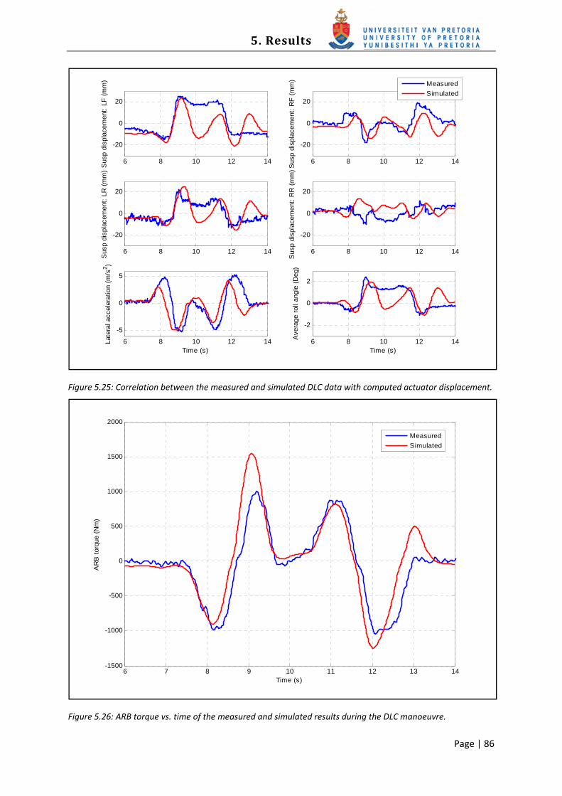
5. Results
Page | 86
Figure 5.25: Correlation between the measured and simulated DLC data with computed actuator displacement.
Figure 5.26: ARB torque vs. time of the measured and simulated results during the DLC manoeuvre.
6 8 10 12 14
-20
0
20S
usp
disp
lace
men
t: LF
(mm
)
6 8 10 12 14
-20
0
20
Sus
p di
spla
cem
ent:
RF
(mm
)
6 8 10 12 14
-20
0
20
Sus
p di
spla
cem
ent:
LR (m
m)
6 8 10 12 14
-20
0
20
Sus
p di
spla
cem
ent:
RR
(mm
)
6 8 10 12 14
-5
0
5
Late
ral a
ccel
erat
ion
(m/s
2 )
Time (s)6 8 10 12 14
-2
0
2
Ave
rage
roll
angl
e (D
eg)
Time (s)
MeasuredSimulated
6 7 8 9 10 11 12 13 14-1500
-1000
-500
0
500
1000
1500
2000
Time (s)
AR
B to
rque
(Nm
)
MeasuredSimulated

5. Results
Page | 87
The final adjustment made was to add friction to the chassis of the model. This was done to model the friction at each suspension strut to improve correlation. The friction was modelled by adding two dummy bodies (with no mass or inertia) to each suspension strut. These dummy bodies were used to be able to model the correct joint configuration so that it does not influence the kinematics of the suspension system. The top dummy bodies were connected by means of a spherical joint to the body of the vehicle. The top and bottom dummy bodies were connected with translational joints to each other, while the bottom dummy bodies were connected with hooks joints to the axles.
Friction was imposed on the four translational joint by using the built in friction function of ADAMS. The static and dynamic friction coefficients were set to 0.01 so that their effects are neglectable. This was done because the normal force on this joint is unknown and is not a representation of the friction that is in the system. The friction was modelled by adding a preload that has to be overcome before the joint will move and there after the friction remains constant. Values of 0, 200, 400, 600 and 800 N were used to determine the sensitivity of the system for this parameter. This was done for the constant radius test with the passive ARB as well as the DLC manoeuvre with the ARB disconnected. These two test runs were chosen because this parameter has the largest influence on the results during these runs. The result of the constant radius test is shown in Figure 5.27 and for the DLC manoeuvre is given in Figure 5.28 for the different friction values. The measured results are also shown in the graphs to give the reference value for the test.
Figure 5.27: Effect of friction on the model during a constant radius test.
-2 -1 0 1 2 3 4 5 6 7 8-1
0
1
2
3
4
5
6
7
Lateral acceleration (m/s2)
Rol
l ang
le (D
eg)
Measured resultsSimulation: Zero FrictionSimulation: 200N FrictionSimulation: 400N FrictionSimulation: 600N FrictionSimulation: 800N Friction

5. Results
Page | 88
Figure 5.28: Effect of friction on the model during a DLC manoeuvre.
From these results it can be concluded that by adding friction to the model increases the correlation of the model. From Figure 5.27 it is shown that the optimal friction for the constant radius test is about 800 N. For the DLC manoeuvre the optimal friction value are given in Figure 5.28 as 200 N. Because these two optimal values are not the same is a sign that this is not the correct way to model this friction in the model and that this must be altered.
It must also be kept in mind that the maximum friction force (800 N) that was added is about 11% of the maximum force in the struts and has a 72% influence on the results of the DLC manoeuvre. So the model is very sensitive to this parameter and can have a major impact on the simulation results.
It was decided to model the friction with a graph as shown in Figure 5.29, where the peak of the graph is at 800 N and the flat part of the graph is at 200 N. This is a typical way stick slip is modelled in simulations. It was also decided to remove the previously modelled friction and insert the new modified friction by adding it to the damping force which is calculated in Matlab. This makes it easier to adjust this graph as needed. Adding this modified friction force to the model resulted in some numerical problems during the simulations, especially during the constant radius test. This was due to the sharp inclines and peaks of the modified friction graph which presents a large discontinuity. This problem was overcome by decreasing the slopes of the modified friction graph and using a very small step size (0.0002 s) for the simulations.
The results of adding the modified friction to the model are shown in Figure 5.30 for the constant radius test and in Figure 5.31 for the DLC manoeuvre.
2 3 4 5 6 7 8 9 10 11-6
-5
-4
-3
-2
-1
0
1
2
3
4
5
Time (s)
Rol
l ang
le (D
eg)
Measured resultsSimulation: Zero FrictionSimulation: 200N FrictionSimulation: 400N FrictionSimulation: 600N FrictionSimulation: 800N Friction

5. Results
Page | 89
Figure 5.29: Graph of how the modified friction is modelled.
Figure 5.30: Effect of modified friction on the model during a constant radius test.
-0.2 -0.15 -0.1 -0.05 0 0.05 0.1 0.15 0.2
-800
-600
-400
-200
0
200
400
600
800
Velocity (m/s)
Fric
tion
forc
e (N
)
-2 -1 0 1 2 3 4 5 6 7 8-0.5
0
0.5
1
1.5
2
2.5
3
3.5
4
Lateral acceleration (m/s2)
Rol
l ang
le (D
eg)
Measured resultsSimulation: 800N FrictionSimulation: Modified Friction

5. Results
Page | 90
Figure 5.31: Effect of modified friction on the model during a DLC manoeuvre.
Good correlation is found between the constant friction and the modified friction models. This shows that the modified friction graph is a successful way to model the friction in the chassis and suspension members of the vehicle. The modified friction graph can be fine‐tuned further to improve correlation for future work.
5.8 Conclusion
The following is concluded based on the evidence provided in this chapter:
• Three tests were performed to measure the performance of the system: o Constant radius test o Double‐lane‐change‐test o Ride comfort test over Belgian paving
• Three test sessions were conducted so that adjustments could be made after each test session.
• The final results show that: o The average body roll angle is reduced to zero up to a lateral acceleration of 0.4 g
during steady state cornering. o The average body roll angle is reduced by 74% during the DLC manoeuvre at 70
km/h over the baseline vehicle with the soft suspension setting.
2 3 4 5 6 7 8 9 10 11-6
-5
-4
-3
-2
-1
0
1
2
3
4
5
Time (s)
Rol
l ang
le (D
eg)
Measured resultsSimulation: 200N FrictionSimulation: Modified Friction

5. Results
Page | 91
o No change is noticed in the ride comfort of the vehicle with and without the system.
• Modifications were made to the simulation model to improve correlation with the measured results.
Page | 92
6 Conclusion
The literature study revealed several concepts with the potential to improve the handling of off‐road vehicles. These concepts include passive suspensions, semi‐active suspensions, active anti‐roll bar systems, active suspensions and tilting vehicles. These solutions were weighted according to the same criteria and the active anti‐roll bar system was identified as the most suitable solution.
It was decided to perform three types of tests to quantify any improvements in vehicle handling. These tests include steady state handling (constant radius test), dynamic handling (double‐lane‐change‐test) and ride comfort tests (drive over the Belgian paving at constant speed). The maximum body roll angle was used to quantify the handling of the vehicle during the handling tests. During the ride comfort tests, the weighted RMS of the vertical acceleration measured on the body of the vehicle was used to quantify the ride comfort of the vehicle.
An existing ADAMS model of the test vehicle (Land Rover Defender 110) was taken and double‐lane‐change‐manoeuvres were done to predict the response of the vehicle. This was evaluated against double‐lane‐change‐tests done with the baseline vehicle before any modifications were done. The ADAMS model was modified until good correlation was achieved.
The active anti‐roll bar system was modelled in ADAMS and predicted results were obtained. These simulations also provided values for key design variables. After all the design variables had been finalised, the whole active anti‐roll bar system was designed in Solid Works. From these CAD models drawings were created that was used to manufacture all the components. The torsional stiffness of the anti‐roll bar was measured to check the calculations and to determine the torsional stiffness of the anti‐roll bar. The system was implemented on the test vehicle and correct operation was verified. The test vehicle was instrumented with the required sensors and prepared for testing.
Tests were done at Gerotek Test Facilities. The active anti‐roll bar system responded exactly as expected during a constant radius test by cancelling out the body roll of the vehicle up to a lateral acceleration of 0.4 g and from there increase with the same amount as the passive anti‐roll bar. The active anti‐roll bar system showed a decrease in maximum body roll angle of up to 74% over the baseline vehicle during the double‐lane‐change‐manoeuvre at 70 km/h where the simulations predicted an 80% improvement. This system also showed no detrimental effect on the ride comfort of the vehicle.
Finally, the ADAMS model was adjusted to improve correlation with the active anti‐roll bar system.
This thesis concludes that the active anti‐roll bar system can dramatically improve the handling of an off‐road vehicle without the sacrifice of ride comfort.

Page | 93
7 Future work
The following topics need to be addressed in future work:
• The tyre model used in the simulations is under suspicion. It was found that if the vertical wheel load transfer is too large, the tyre model does not give the same results as the measured results. This shows that there is a need for an improved tyre model or improved tyre characteristics for the current tyre model (Pacejka ’89). Another area where the current tyre model might be insufficient is where handling simulations are done on rough roads. This is difficult to prove due to the fact that no tests could be conducted to obtain results, but it is highly unlikely that the current tyre model will be sufficient for these conditions.
• Simulation done in this thesis (Par. 5.7) showed that adding friction to the chassis of the simulation model increases the correlation of the model with the measured results. This friction has a large influence on the results of the simulations. This modified friction graph can be altered to improve correlation with the test vehicle.
• Tests done in this thesis (Par. 5.4.3) show that ride comfort can be improved with an AARB system. Further work can be done on how exactly this can be achieved and to incorporate it with the AARB developed in this thesis and the rest of the vehicle. This however, must be done without the sacrifice of handling.
• The test vehicle can be automated so that tests can be conducted with the same software used in the simulations to calculate the desired steering angle. This will dramatically increase the repeatability of the tests and make it easier to predict the results of a manoeuvre with simulations and to reconstruct tests done with the simulations.
• Active body control can be done with the 4S4 by adding rapid height adjustment. These modifications on the 4S4 will change this semi‐active suspension system to an active suspension system. This will open a whole new development area for future work.
• During this study an AARB was added only to the rear of the vehicle due to space constraints. As shown, this increases the handling ability of the vehicle, but it also decreases the yaw stability of the vehicle. This is due to the AARB increasing the lateral load transfer on the rear axle which will cause the lateral forces generated by the rear axle to saturate most likely before the lateral forces generated by the front axle. This condition will cause the vehicle to spin out (limited oversteer) and can be improved by adding an AARB to the rear axle as well as to the front axle. This aspect is open for future investigation.

Page | 94
8 Bibliography
Ahmadian, M. and Simon, D. E., 2004, Can semiactive dampers with skyhook control improve roll stability of passenger vehicles?, SAE Technical Paper 2004‐01‐2099, Society of Automotive Engineers, Warrendale.
Bakker, E., Pacejka, H. B. and Lidner, L., 1989, A new tyre model with an application in vehicle dynamics studies, SAE Technical Paper 890087, Society of Automotive Engineers, Warrendale.
Becker, C. M., 2008. Profiling of rough terrain, Unpublished M.Eng. Thesis, University of Pretoria, Pretoria, South Africa.
British Standards Institution, 1987, British Standard Guide to Measurement and Evaluation of Human Exposure to Whole‐Body Mechanical Vibration and Repeated Shock, BS 6841.
Cimba, D., Wagner, J. and Baviskar, A., 2006, Investigation of active torsion bar actuator configurations to reduce vehicle body roll, Vehicle System Dynamics, Volume 44, Number 9, 2006, pp. 719‐736.
Danesin, D., Krief, P., Sorniotti, A. and Velardocchia, M., 2003, Active roll control to increase handling and comfort, SAE Technical Paper 2003‐01‐0962, Society of Automotive Engineers, Warrendale.
Darling, J. and Hickson, L. R., 1998, An experimental study of a prototype active anti‐roll suspension system, Vehicle System Dynamics, Volume 29, Number 5, 1998, pp. 309‐329.
Darling, J. and Rosam, N., 1996, The interconnected hydragas roll control active suspension, Proceedings of the ASME International Mechanical Engineers Congress & Exhibition, Atlanta, 17‐22 November 1996.
Darling, J., Dorey, R. E. and Ross‐Martin, T. J., 1992, A Low cost active anti‐roll suspension for passenger cars, Journal of Dynamic Systems, Measurement and Control, Volume 114, December 1992, pp. 599‐605.
Dukkipati, R. V., Pang, J., Qatu, M. S., Sheng, G. and Shuguang, Z., 2008, Road vehicle dynamics, Society of Automotive Engineers, Warrendale, PA.
Els, P. S., 2006, The ride comfort vs. handling compromise for off‐road vehicles, Unpublished PhD thesis, University of Pretoria, Pretoria, South Africa, http://upetd.up.ac.za/thesis/available/etd‐07152008‐102911/, Accessed: 4 February 2008.
Everett, N. R., Brown, M. D. and Crolla, D. A., 2000, Investigation of a roll control system for an off‐road vehicle, SAE Technical Paper 2000‐01‐1646, Society of Automotive Engineers, Warrendale.
Forkenbrock, G. J., O’Harra, B. C. and Elsasser, D., 2004, A demonstration of the dynamic tests developed for NHTSA’s NCAP rollover rating system: Phase VIII of NHTSA’s light vehicle research program, US Department of Transportation, DOT HS 809 705

8. Bibliography
Page | 95
Gere, J. M., 2004, Mechanics of materials, Volume 6, Thomson Learning, Belmont, USA.
Gerotek Test Facilities, 2008, Gerotek Test Facilities, http://www.armscorbusiness.com/SubSites/Gerotek/Gerotek01_landing.asp, Accessed: 1 October 2008.
Gillespie, T. D., 1992. Fundamentals of vehicle dynamics, Society of Automotive Engineers, Inc., Warrendale, PA.
Gohl, J., Rajamani, R., Alexander, L. and Starr, P., 2004, Active roll mode control implementation on a narrow tilting vehicle, Vehicle System Dynamics, Volume 42, Number 5, 2004, pp. 347‐372.
Haubenreich, R. W. and Law, E. H., 2000, An investigation into the effects of suspension tuning on the cornering of a Winston cup race car, SAE Technical Paper 2000‐01‐3569, Society of Automotive Engineers, Warrendale.
Hubert, K. and Kumar, A., 2005, Anti‐roll stability suspension technology, SAE Technical Paper 2005‐01‐3522, Society of Automotive Engineers, Warrendale.
International Organisation for Standardisation, 1975, International Standard ISO 3888‐1975: Road vehicles – test procedure for a severe lane‐change manoeuvre, ISO/TR 3888‐1975.
Kim, H. J. and Park, Y. P., 2004, Investigation of robust roll motion control considering varying speed and actuator dynamics, Mechatronics, Volume 14, 2004, pp. 35‐54.
Kim, W., Lee, J., Yoon, S. and Kim, D., 2005, Development of Mando's new continuously controlled semi‐active suspension system, SAE Technical Paper 2005‐01‐1721, Society of Automotive Engineers, Warrendale.
Midrand Special Steels, 2008, Midrand special steels datasheet, Centurion, South Africa.
MSC ADAMS Help, 2007, Introduction to ADAMS Tyre, file:///C:/MSC.Software/MSC.ADAMS/2007r1/help/wwhelp/wwhimpl/js/html/wwhelp.htm, Accessed: 15 September 2008.
Packer, M. B., 1978, Active ride control ‐ a logical step from static vehicle attitude, SAE Technical Paper 780050, Society of Automotive Engineers, Warrendale.
Shuttlewood, D. W., Crolla, D. A., Sharp, R. S. and Crawford, I. L., 1993, Active roll contol for passenger cars, Vehicle system dynamics, Volume 22, 1993, pp. 383‐396.
Sorniotti, A., 2006, Electro‐mechanical active roll control: a new solution for active suspension, SAE Technical Paper 2006‐01‐1966, Society of Automotive Engineers, Warrendale.
Stone Hydraulics, 2008, Pick‐A‐Pack, http://www.stonehydraulics.com/pickapack.aspx, Accessed: 16 September 2008.
Thoresson, M. J., 2007, Efficient gradient‐based optimisation of suspension characteristics for an off‐road vehicle, Unpublished PhD thesis, University of Pretoria, Pretoria, South Africa, http://upetd.up.ac.za/thesis/available/etd‐08042008‐093103/, Accessed: 17 March 2008.

8. Bibliography
Page | 96
Tillback, L. R. and Brodd, S., 1989, Active suspension ‐ the Volvo experience, SAE Technical Paper 890083, Society of Automotive Engineers, Warrendale.
Trelleborg Sealing Solutions, 2007, Hydraulic Seals ‐ linear metric version (complete catalog), http://www.tss.trelleborg.com/com//www/media/downloads/catalogs/hydraulic_complete_gb.pdf, Accessed: 14 February 2008.
Uys, B. P., 2007, “Omrol van veldvoertuie”, Rollover of off‐road vehicles, Unpublished M.Eng Thesis, University of Pretoria, Pretoria, South Africa, http://upetd.up.ac.za/thesis/available/etd‐06032008‐113745/, Accessed: 6 May 2008.
Uys, P. E., Els, P. S. and Thoresson, M. J., 2004, Criteria for handling measurement, Journal of Terramechanics, Volume 43, 2006, pp. 43‐67.
Uys, P. E., Els, P. S., Thoresson, M. J., Voigt, K. G. and Combrinck, W. C., 2006, Experimental determination of moments of inertia for an off‐road vehicle in a regular engineering laboratory, International Journal of Mechanical Engineering Education, Volume 34, Number 4, pp. 291‐314.
Wilde, J. R., Heydinger, G. J., Guenther, D. A., Mallin, T. and Devenish, A. M., 2005, Experimental evaluation of fishhook maneuver performance of a kinetic suspension system, SAE Technical Paper 2005‐01‐0392, Society of Automotive Engineers, Warrendale.
Yoon, S., Jung, J., Koo, B. and Kim, D., 2006, Development of rollover prevention system using Unified Chassis Control of ESP and CDC systems, SAE Technical Paper 2006‐01‐1276, Society of Automotive Engineers, Warrendale.