MATHEMATICAL BIOSCIENCES doi:10.3934/mbe.2012.9.297AND ENGINEERINGVolume 9, Number 2, April 2012 pp. 297–312

GLOBAL STABILITY FOR EPIDEMIC MODEL WITH

CONSTANT LATENCY AND INFECTIOUS PERIODS

Gang Huang

School of Mathematics and Physics

China University of Geosciences, Wuhan, 430074, China

Edoardo Beretta

CIMAB, University of Milano

via C. Saldini 50, I 20133 Milano, Italy

Yasuhiro Takeuchi

Graduate School of Science and TechnologyShizuoka University, Hamamatsu, 4328561, Japan

(Communicated by Jia Li)

Abstract. In recent years many delay epidemiological models have been pro-

posed to study at which stage of the epidemics the delays can destabilize the

disease free equilibrium, or the endemic equilibrium, giving rise to stabilityswitches. One of these models is the SEIR model with constant latency time

and infectious periods [2], for which the authors have proved that the two de-lays are harmless in inducing stability switches. However, it is left open the

problem of the global asymptotic stability of the endemic equilibrium whenever

it exists. Even the Lyapunov functions approach, recently proposed by Huangand Takeuchi to study many delay epidemiological models, fails to work onthis model. In this paper, an age-infection model is presented for the delay

SEIR epidemic model, such that the properties of global asymptotic stabilityof the equilibria of the age-infection model imply the same properties for the

original delay-differential epidemic model. By introducing suitable Lyapunov

functions to study the global stability of the disease free equilibrium (whenR0 ≤ 1) and of the endemic equilibria (whenever R0 > 1) of the age-infection

model, we can infer the corresponding global properties for the equilibria ofthe delay SEIR model in [2], thus proving that the endemic equilibrium in [2]is globally asymptotically stable whenever it exists.

Furthermore, we also present a review of the SIR, SEIR epidemic models,with and without delays, appeared in literature, that can be seen as particular

cases of the approach presented in the paper.

2000 Mathematics Subject Classification. Primary: 92D30, 34A34; Secondary: 34D20, 34D23.

Key words and phrases. Global stability, epidemic model, infectious period, age-structure.This research is partially supported by National Basic Research Program of China (973 Pro-

gram), No. 2011CB710602, 604.

297

298 GANG HUANG, EDOARDO BERETTA AND YASUHIRO TAKEUCHI

1. Previous results. In the paper [2], Beretta and Breda study a two-delays SEIRepidemic model as follows:

dS(t)

dt= Λ− µ1S(t)− g(I(t))S(t),

dE(t)

dt= g(I(t))S(t)− g(I(t− τ1))S(t− τ1)e−µ2τ1 − µ2E(t),

dI(t)

dt= g(I(t− τ1))S(t− τ1)e−µ2τ1 (1.1)

− g(I(t− τ1 − τ2))S(t− τ1 − τ2)e−µ2(τ1+τ2) − µ2I(t),

dR(t)

dt= g(I(t− τ1 − τ2))S(t− τ1 − τ2)e−µ2(τ1+τ2) − µ3R(t).

In the SEIR model (1.1), they have assumed that the exposed individuals E(t), whoare infected but not yet infectious, have a latency time τ1, after which they becomeinfectious I(t) (i.e. capable to infect susceptibles S(t)) and have an infectious periodτ2. Both exposed and infectious individuals are assumed to have the same deathrate “µ2”, whereas the susceptibles have a natural death rate constant “µ1”. Atthe end of the infectious period, i.e. at the infection age a = τ1 + τ2, it is assumedthat the infected individuals are removed from the infection, thus entering in theclass of the removed individuals R(t), which have a proper death rate constant“µ3”. Furthermore, for the nonlinear incidence rate g(I), the structure g(I) =βI

1+αI , α, β ∈ R+ was chosen.

The initial conditions for model (1.1), by biological reasons, are the positivecontinuous functions:

S(θ) = ψ1(θ), I(θ) = ψ2(θ), θ ∈ [−(τ1 + τ2), 0], (1.2)

with S(0), R(0) ≥ 0. Moreover, since E(t), I(t) in (1.1) can be written as:

E(t) =

∫ τ1

0

g(I(t− a))S(t− a)e−µ2ada,

I(t) =

∫ τ1+τ2

τ1

g(I(t− a))S(t− a)e−µ2ada,

then, by continuity E(0), I(0) must satisfy that :

E(0) =

∫ τ1

0

g(I(−a))S(−a)e−µ2ada, I(0) =

∫ τ1+τ2

τ1

g(I(−a))S(−a)e−µ2ada.

(1.3)The delay model (1.1) has two equilibria: the disease-free equilibrium (DFE) E0

= (S0 = Λµ1, E0 = 0, I0 = 0, R0 = 0), which exists for all the parameter values, and

the positive equilibrium E∗ = (S∗, E∗, I∗, R∗) which exists if and only if the basicreproduction number

R0 =1

µ2

Λ

µ1· g′(0)e−µ2τ1(1− e−µ2τ2),

satisfies R0 > 1 , since it can be proven that its components are:

S∗ =Λ

µ1 + g(I∗), E∗ =

1

µ2g(I∗)S∗(1− e−µ2τ1),

I∗ =1

µ2g(I∗)S∗e−µ2τ1(1− e−µ2τ1), R∗ =

1

µ3g(I∗)S∗e−µ2(τ1+τ2),

GLOBAL STABILITY FOR EPIDEMIC MODEL 299

In [2], both by the analysis of the characteristic equations and by the iterativeschemes coupled with the comparison principle for differential equations, the fol-lowing dynamical properties for model (1.1), with i.c. (1.2), were obtained:

Theorem 1.1. If R0 ≤ 1 the DFE E0 is globally attractive, i.e. for all initialconditions limt→∞(S(t), E(t), I(t), R(t)) = ( Λ

µ1, 0, 0, 0).

Theorem 1.2. If R0 > 1, the DFE E0 is unstable.

Theorem 1.3. The positive equilibrium E∗ is globally attractive if “ βα < µ1”.

Theorem 1.4. The system (1.1) is permanent if R0 > 1 and “βα < µ1”.

Theorem 1.5. Whenever it exists, the positive equilibrium E∗ is locally asymptot-ically stable.

As already noticed in [2], the results in Theorems 1.1.-1.5. show that boththe delays are harmless in inducing stability switches at both the equilibria E0

and E∗. However, since the basic reproductive number R0 depends upon boththe latency time τ1 and on the infectivity period τ2, even the existence conditionR0 > 1 of the positive equilibrium E∗, jointly with the stability properties of E0 ,will be dependent upon both delays. The latency time and the infectivity periodhowever play an opposite role on the existence of the endemic equilibrium E∗ (wesay E∗ to be endemic iff we can prove that whenever R0 > 1 then E∗ is globallyasymptotically stable): while the condition R0 > 1 requires that the latency timeτ1 must be sufficiently small in order that

τ1 < h(τ2) :=1

µ2ln

[βΛ

µ1µ2(1− e−µ2τ2)

],

on the opposite side, the infectivity period must be sufficiently large to ensure that:

τ2 > τ∗2 :=1

µ2ln

[βΛ

βΛ− µ1µ2

].

Furthermore, it is evident from the condition τ1 < h(τ2) that there is a thresholdfor the latency time, say

τ∗1 :=1

µ2ln

[βΛ

µ1µ2

],

such that if τ1 > τ∗1 the condition R0 > 1 cannot be realized whatever large theinfectivity period τ2 is.

Returning to the asymptotic stability of the positive equilibrium E∗, we see thatTheorems 1.3. and 1.5. only imply its global asymptotic stability if “βα < µ1”.Hence, it is interesting to see wether it is possible to prove the global asymptoticstability of the endemic equilibrium E∗ whenever it exists (R0 > 1). This is one ofthe main targets of this paper.

Recently, many researchers studied delay epidemic models by using Lyapunovapproach and achieve nice results on global stability of equilibria (e.g., [6, 7, 8, 18]).In [7, 8], Huang and Takeuchi employed a class of Goh-type Lyapunov functionsthat integrate over past states to establish global stability for delay SIR, SEIR,SEI, SIS epidemiological models with a general incidence rate. However, in themodels appearing in the above mentioned papers the delay terms appeared withpositive signs and this is an essential feature to ensure that the related Lyapunovfunctionals work well. However, in the model (1.1) two delay terms appear with

300 GANG HUANG, EDOARDO BERETTA AND YASUHIRO TAKEUCHI

negative signs. Correspondingly, the typical Lyapunov functions in [7, 8] do notwork for the model (1.1). Hence, the global asymptotic stability of the positiveequilibrium E∗ by Lyapunov functionals is left as open question in [2].

In this paper, in Section 2 we reformulate the above delay differential equationsmodel with nonlinear incidence as an equivalent age-infection model with nonlinearboundary conditions, which implies the stability properties of (1.1). In Section3, by using Lyapunov function approach for age-structured models [9, 14, 15], weestablish the global stability of the endemic equilibrium of the delay model (1.1).Furthermore, in Section 4, we prove that our approach by Lyapunov functionsapplied to infection age-structured models can be applied to a wide class of delay-differential models.

2. Reformulating the delay model as an age-structured model. To refor-mulate the delay-differential model (1.1) we introduce the density i(t, a) at time tof infected individuals with infection age a, where the variable a measures, at timet, the duration for which the individuals have been infected. According to the SEIRmodel (1.1), we define:

E(t) =

∫ τ1

0

i(t, a)da, I(t) =

∫ τ1+τ2

τ1

i(t, a)da, (2.1)

whereas, the balance equation for the removed individuals R(t) is

dR(t)

dt= i(t, τ1 + τ2)− µ3R(t). (2.2)

Thus, the age-structured model corresponding to the delay-differential model(1.1) is:

ddtS(t) = Λ− µ1S(t)− i(t, 0),∂∂t i(t, a) + ∂

∂a i(t, a) = −µ2i(t, a),

+b.c. i(t, 0) = g(I(t))S(t).

+i.c. i(0, a) = ψ(a), a ∈ [0, a],

(2.3)

jointly with the equations (2.1) and (2.2).It is to be noticed that, once known the initial condition (1.2) for system (1.1), the

initial condition ψ(a), a ∈ [0, a] for the age model (2.3) is also given and, accordingto (1.2), satisfies the continuity condition (1.3) for E(0), I(0). This initial conditionis:

ψ(a) := g(ψ2(−a))ψ1(−a) exp(−µ2a), a ∈ [0, a]. (2.4)

Now , it is well known (see [5] [13]) that the solution of the Lotka-McKendricequation:

∂∂t i(t, a) + ∂

∂a i(t, a) = −µ(a)i(t, a),

i(t, 0) = B(t) := g(I(t))S(t),

i(0, a) = ψ(a), a ∈ [0, a],

(2.5)

where ψ(a), a ∈ [0, a], is the initial condition (2.4), exists and it is unique for all(t, a) ∈ (0,+∞)× [0, a].

Once introduced the “survival probability Π(a) = exp(−∫ a

0µ(ν)dν)”, the solu-

tion is given by:

i(t, a) =

{ψ(a− t) Π(a)

Π(a−t) if a ≥ t,B(t− a)Π(a) if a < t.

GLOBAL STABILITY FOR EPIDEMIC MODEL 301

Since for system (2.3) we have Π(a) = exp(−µ2a), then the solution to system(2.3) with i.c. (2.4) becomes:

i(t, a) =

{g(ψ2(−(a− t)))ψ1(−(a− t))Π(a− t) Π(a)

Π(a−t) if a ≥ t,g(I(t− a))S(t− a)Π(a) if a < t.

(2.6)

Hence, in synthesis, the solution (2.6) can be written as:

i(t, a) = g(I(t− a))S(t− a) exp(−µ2a) for all t ≥ 0 and a ∈ [0, a], (2.7)

where, according to the initial conditions for the delay system (1.1), it is:

S(t− a) = ψ1(t− a), I(t− a) = ψ2(t− a), whenever t− a ∈ [−a, 0].

Now, thanks to (2.7), we want to show that the age model (2.3) with (2.1), (2.2)is equivalent to the delay-differential SEIR model (1.1) in the sense that, any ofits solution (S(t), E(t), I(t), R(t)), t ≥ 0, is also solution of system of the delay-differential system (1.1) with initial conditions (1.2).

From (2.1) and (2.2), we have

dE(t)

dt=

d

dt

∫ τ1

0

i(t, a)da =

∫ τ1

0

∂

∂ti(t, a)da

= −∫ τ1

0

(∂

∂ai(t, a) + µ2i(t, a)

)da

= − i(t, a) |τ10 −µ2

∫ τ1

0

i(t, a)da

= i(t, 0)− i(t, τ1)− µ2E(t),

that thanks to (2.7) gives

dE(t)

dt= g(I(t))S(t)− e−µ2τ1 · g(I(t− τ1))S(t− τ1)− µ2E(t).

Similarly, we have

dI(t)

dt=

d

dt

∫ τ1+τ2

τ1

i(t, a)da = i(t, τ1)− i(t, τ1 + τ2)− µ2I(t)

= e−µ2τ1 · g(I(t− τ1))S(t− τ1)

− e−µ2(τ1+τ2) · g(I(t− τ1 − τ2))S(t− τ1 − τ2)− µ2I(t),

and finally

dR(t)

dt= i(t, τ1 + τ2)− µ3R(t) = e−µ2(τ1+τ2)i(t− (τ1 + τ2), 0)− µ3R(t)

= e−µ2(τ1+τ2) · g(I(t− (τ1 + τ2)))S(t− (τ1 + τ2))− µ3R(t).

The above three equations are identical to the last three delay-differential equa-tions in system (1.1). Hence, we have the following:

Proposition 1. The model (1.1) is implied by the age-structured model (2.3) with(2.1) and (2.2) in the sense that, for all t ≥ 0, any of its solutions (S(t), E(t), I(t),R(t)) is also solution of the delay-differential system (1.1).

302 GANG HUANG, EDOARDO BERETTA AND YASUHIRO TAKEUCHI

3. Global stability of the age-structured model (2.3). The equilibria E =(S∗, i∗(a)), a ∈ [0, a] of the age-structured model (2.3) with (2.1) and (2.2) aresolutions of {

Λ− µ1S − i(0) = 0,dda i(a) = −µ2i(a), i(0) = g(I)S, a ∈ [0, a],

(3.1)

where, according to (2.1), the other equilibrium components are given by

E∗ =

∫ τ1

0

i∗(a)da, I∗ =

∫ τ1+τ2

τ1

i∗(a)da, R∗ =i∗(τ1 + τ2)

µ3. (3.2)

We see that the trivial equilibrium of model (2.3) is the disease-free equilibrium

E0 = (S0, i0(a)) =

(Λ

µ1, 0

), a ∈ [0, a],

which, according to (3.2), corresponds to the disease-free equilibrium E0 = (Λ/µ1, 0,0, 0) of system (1.1).

Besides E0, system (2.3) has the positive equilibrium

E∗ = (S∗ =Λ

µ1 + g(I∗), i∗(a)), a ∈ [0, a],

where

i∗(a) = g(I∗)S∗e−µ2a, a ∈ [0, a].

According to (3.1) and (3.2), S∗, I∗ is the unique positive solution of{Λ− µ1S

∗ − g(I∗)S∗ = 0,

µ2I∗ = g(I∗)S∗(e−µ2τ1 − e−µ2(τ1+τ2)),

(3.3)

which exist if and only if the basic reproduction number R0 of system (1.1) is:R0 > 1. Of course, according (3.2) the equilibrium E∗ corresponds to the positiveequilibrium E∗ of system (1.1).

For the sake of simplicity, in the following, by referring to the equilibria E0 andE∗ we will leave out the information a ∈ [0, a].

Proposition 2. The age-infection model (2.3) has always the disease-free equi-librium E0(Λ/µ1, i0(a)). In addition, there exists a unique positive equilibriumE∗(S∗, i∗(a)) when R0 > 1.

In the following, we would study the stability of equilibria of the age-infectionmodel (2.3) by Lyapunov functions.

Theorem 3.1. When R0 ≤ 1, the equilibrium E0 = (Λ/µ1, 0) is globally asymptot-ically stable.

Proof. Firstly, we define two non-negative functions:

(i), φ(a) = (1− e−µ2τ2)eµ2(a−τ1) for a ∈ [0, τ1]. We have

φ(0) = (1− e−µ2τ2)e−µ2τ1 ,

φ(τ1) = 1− e−µ2τ2 ,

φ′a(a) =d

daφ(a) = µ2φ(a).

GLOBAL STABILITY FOR EPIDEMIC MODEL 303

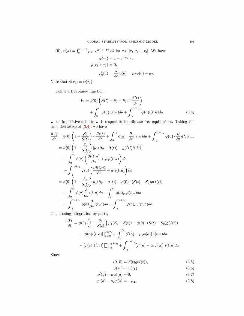
(ii), ϕ(a) =∫ τ1+τ2a

µ2 · eµ2(a−θ) dθ for a ∈ [τ1, τ1 + τ2]. We have

ϕ(τ1) = 1− e−µ2τ2 ,

ϕ(τ1 + τ2) = 0,

ϕ′a(a) =d

daϕ(a) = µ2ϕ(a)− µ2.

Note that φ(τ1) = ϕ(τ1).

Define a Lyapunov function

V1 = φ(0)

(S(t)− S0 − S0 ln

S(t)

S0

)+

∫ τ1

0

φ(a)i(t, a)da+

∫ τ1+τ2

τ1

ϕ(a)i(t, a)da, (3.4)

which is positive definite with respect to the disease free equilibrium. Taking thetime derivative of (3.4), we have

dV1

dt= φ(0)

(1− S0

S(t)

)· dS(t)

dt+

∫ τ1

0

φ(a) · ∂∂ti(t, a)da+

∫ τ1+τ2

τ1

ϕ(a) · ∂∂ti(t, a)da

= φ(0)

(1− S0

S(t)

)[µ1(S0 − S(t))− g(I(t)S(t))]

−∫ τ1

0

φ(a)

(∂i(t, a)

∂a+ µ2i(t, a)

)da

−∫ τ1+τ2

τ1

ϕ(a)

(∂i(t, a)

∂a+ µ2i(t, a)

)da

= φ(0)

(1− S0

S(t)

)µ1(S0 − S(t))− φ(0) · (S(t)− S0)g(I(t))

−∫ τ1

0

φ(a)∂

∂ai(t, a)da−

∫ τ1

0

φ(a)µ2i(t, a)da

−∫ τ1+τ2

τ1

φ(a)∂

∂ai(t, a)da−

∫ τ1+τ2

τ1

ϕ(a)µ2i(t, a)da

Then, using integration by parts,

dV1

dt= φ(0)

(1− S0

S(t)

)µ1(S0 − S(t))− φ(0) · (S(t)− S0)g(I(t))

− [φ(a)i(t, a)]∣∣a=τ1

a=0+

∫ τ1

0

[φ′(a)− µ2φ(a)] i(t, a)da

− [ϕ(a)i(t, a)]∣∣a=τ1+τ2

a=τ1+

∫ τ1+τ2

τ1

[ϕ′(a)− µ2ϕ(a)] i(t, a)da

Since

i(t, 0) = S(t)g(I(t)), (3.5)

φ(τ1) = ϕ(τ1), (3.6)

φ′(a)− µ2φ(a) = 0, (3.7)

ϕ′(a)− µ2ϕ(a) = −µ2, (3.8)

304 GANG HUANG, EDOARDO BERETTA AND YASUHIRO TAKEUCHI

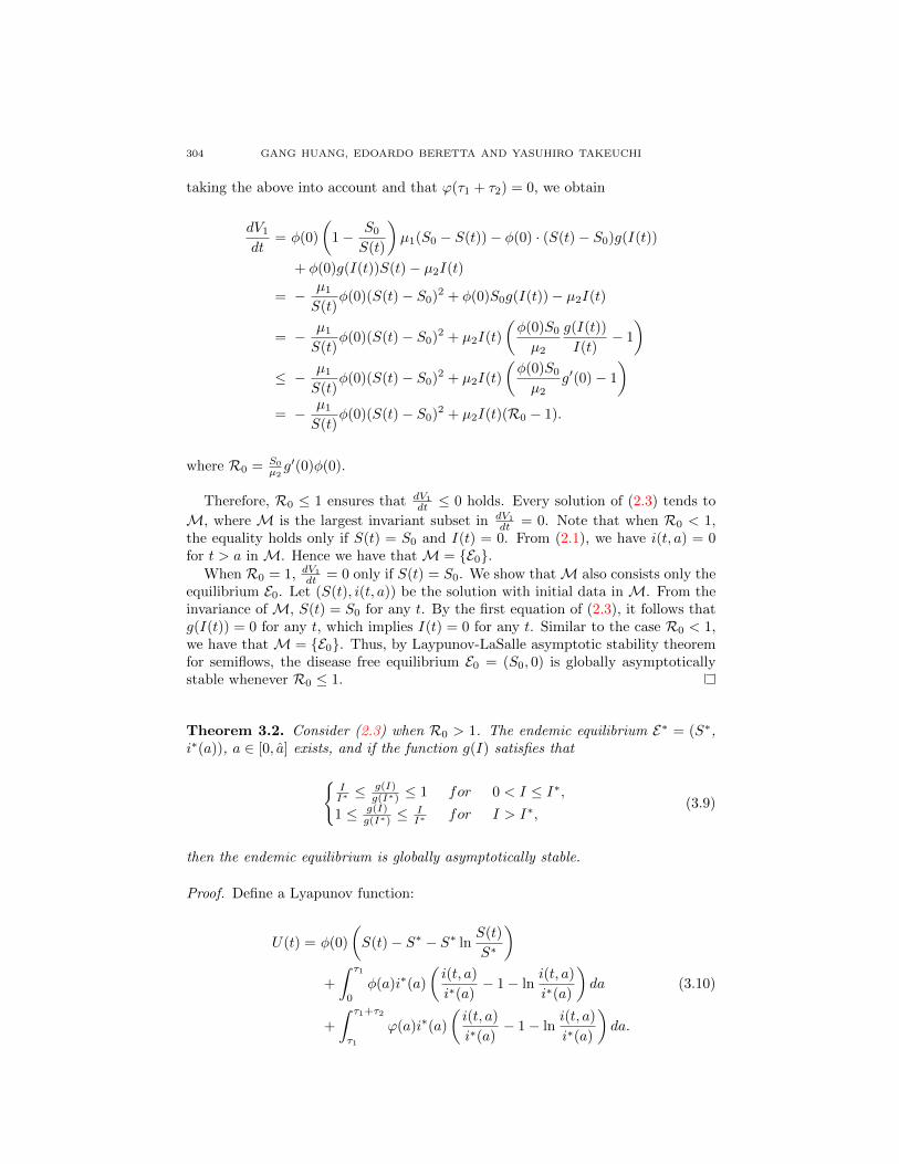
taking the above into account and that ϕ(τ1 + τ2) = 0, we obtain

dV1

dt= φ(0)

(1− S0

S(t)

)µ1(S0 − S(t))− φ(0) · (S(t)− S0)g(I(t))

+ φ(0)g(I(t))S(t)− µ2I(t)

= − µ1

S(t)φ(0)(S(t)− S0)2 + φ(0)S0g(I(t))− µ2I(t)

= − µ1

S(t)φ(0)(S(t)− S0)2 + µ2I(t)

(φ(0)S0

µ2

g(I(t))

I(t)− 1

)≤ − µ1

S(t)φ(0)(S(t)− S0)2 + µ2I(t)

(φ(0)S0

µ2g′(0)− 1

)= − µ1

S(t)φ(0)(S(t)− S0)2 + µ2I(t)(R0 − 1).

where R0 = S0

µ2g′(0)φ(0).

Therefore, R0 ≤ 1 ensures that dV1

dt ≤ 0 holds. Every solution of (2.3) tends to

M, where M is the largest invariant subset in dV1

dt = 0. Note that when R0 < 1,the equality holds only if S(t) = S0 and I(t) = 0. From (2.1), we have i(t, a) = 0for t > a in M. Hence we have that M = {E0}.

When R0 = 1, dV1

dt = 0 only if S(t) = S0. We show thatM also consists only theequilibrium E0. Let (S(t), i(t, a)) be the solution with initial data in M. From theinvariance of M, S(t) = S0 for any t. By the first equation of (2.3), it follows thatg(I(t)) = 0 for any t, which implies I(t) = 0 for any t. Similar to the case R0 < 1,we have that M = {E0}. Thus, by Laypunov-LaSalle asymptotic stability theoremfor semiflows, the disease free equilibrium E0 = (S0, 0) is globally asymptoticallystable whenever R0 ≤ 1.

Theorem 3.2. Consider (2.3) when R0 > 1. The endemic equilibrium E∗ = (S∗,i∗(a)), a ∈ [0, a] exists, and if the function g(I) satisfies that

{II∗ ≤

g(I)g(I∗) ≤ 1 for 0 < I ≤ I∗,

1 ≤ g(I)g(I∗) ≤

II∗ for I > I∗,

(3.9)

then the endemic equilibrium is globally asymptotically stable.

Proof. Define a Lyapunov function:

U(t) = φ(0)

(S(t)− S∗ − S∗ ln

S(t)

S∗

)+

∫ τ1

0

φ(a)i∗(a)

(i(t, a)

i∗(a)− 1− ln

i(t, a)

i∗(a)

)da (3.10)

+

∫ τ1+τ2

τ1

ϕ(a)i∗(a)

(i(t, a)

i∗(a)− 1− ln

i(t, a)

i∗(a)

)da.

GLOBAL STABILITY FOR EPIDEMIC MODEL 305

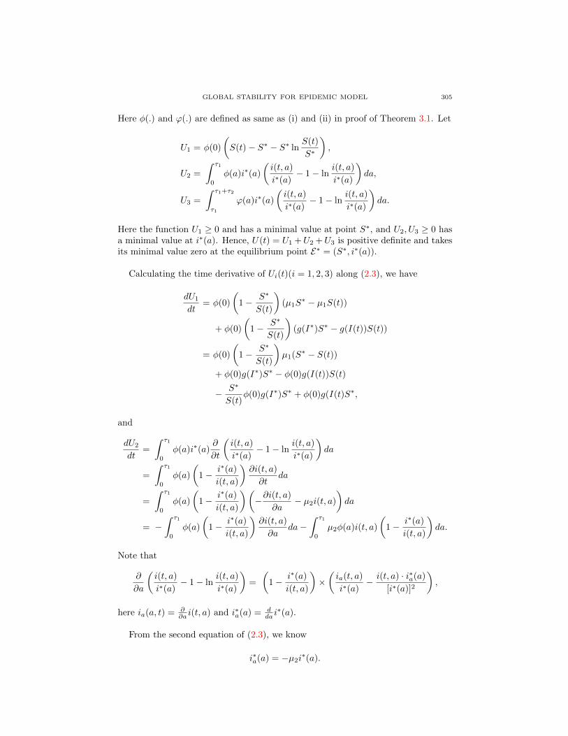
Here φ(.) and ϕ(.) are defined as same as (i) and (ii) in proof of Theorem 3.1. Let

U1 = φ(0)

(S(t)− S∗ − S∗ ln

S(t)

S∗

),

U2 =

∫ τ1

0

φ(a)i∗(a)

(i(t, a)

i∗(a)− 1− ln

i(t, a)

i∗(a)

)da,

U3 =

∫ τ1+τ2

τ1

ϕ(a)i∗(a)

(i(t, a)

i∗(a)− 1− ln

i(t, a)

i∗(a)

)da.

Here the function U1 ≥ 0 and has a minimal value at point S∗, and U2, U3 ≥ 0 hasa minimal value at i∗(a). Hence, U(t) = U1 +U2 +U3 is positive definite and takesits minimal value zero at the equilibrium point E∗ = (S∗, i∗(a)).

Calculating the time derivative of Ui(t)(i = 1, 2, 3) along (2.3), we have

dU1

dt= φ(0)

(1− S∗

S(t)

)(µ1S

∗ − µ1S(t))

+ φ(0)

(1− S∗

S(t)

)(g(I∗)S∗ − g(I(t))S(t))

= φ(0)

(1− S∗

S(t)

)µ1(S∗ − S(t))

+ φ(0)g(I∗)S∗ − φ(0)g(I(t))S(t)

− S∗

S(t)φ(0)g(I∗)S∗ + φ(0)g(I(t)S∗,

and

dU2

dt=

∫ τ1

0

φ(a)i∗(a)∂

∂t

(i(t, a)

i∗(a)− 1− ln

i(t, a)

i∗(a)

)da

=

∫ τ1

0

φ(a)

(1− i∗(a)

i(t, a)

)∂i(t, a)

∂tda

=

∫ τ1

0

φ(a)

(1− i∗(a)

i(t, a)

)(−∂i(t, a)

∂a− µ2i(t, a)

)da

= −∫ τ1

0

φ(a)

(1− i∗(a)

i(t, a)

)∂i(t, a)

∂ada−

∫ τ1

0

µ2φ(a)i(t, a)

(1− i∗(a)

i(t, a)

)da.

Note that

∂

∂a

(i(t, a)

i∗(a)− 1− ln

i(t, a)

i∗(a)

)=

(1− i∗(a)

i(t, a)

)×(ia(t, a)

i∗(a)− i(t, a) · i∗a(a)

[i∗(a)]2

),

here ia(a, t) = ∂∂a i(t, a) and i∗a(a) = d

da i∗(a).

From the second equation of (2.3), we know

i∗a(a) = −µ2i∗(a).

306 GANG HUANG, EDOARDO BERETTA AND YASUHIRO TAKEUCHI

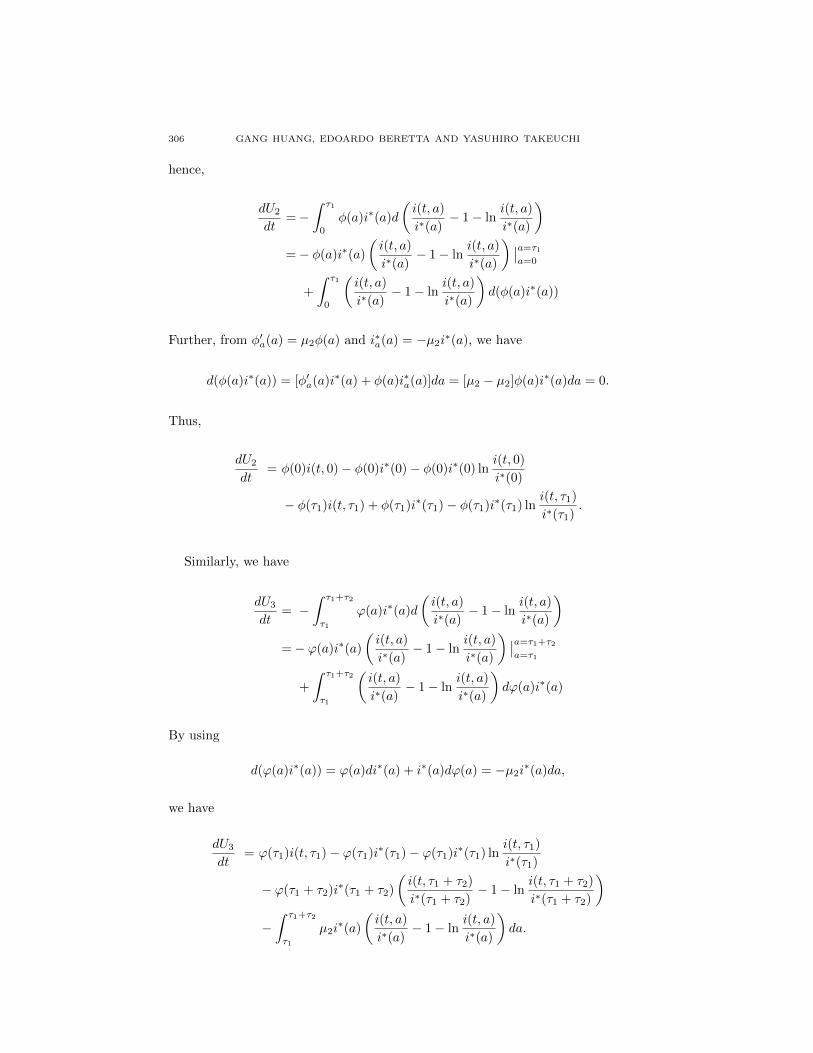
hence,

dU2

dt=−

∫ τ1

0

φ(a)i∗(a)d

(i(t, a)

i∗(a)− 1− ln

i(t, a)

i∗(a)

)=− φ(a)i∗(a)

(i(t, a)

i∗(a)− 1− ln

i(t, a)

i∗(a)

) ∣∣a=τ1

a=0

+

∫ τ1

0

(i(t, a)

i∗(a)− 1− ln

i(t, a)

i∗(a)

)d(φ(a)i∗(a))

Further, from φ′a(a) = µ2φ(a) and i∗a(a) = −µ2i∗(a), we have

d(φ(a)i∗(a)) = [φ′a(a)i∗(a) + φ(a)i∗a(a)]da = [µ2 − µ2]φ(a)i∗(a)da = 0.

Thus,

dU2

dt= φ(0)i(t, 0)− φ(0)i∗(0)− φ(0)i∗(0) ln

i(t, 0)

i∗(0)

− φ(τ1)i(t, τ1) + φ(τ1)i∗(τ1)− φ(τ1)i∗(τ1) lni(t, τ1)

i∗(τ1).

Similarly, we have

dU3

dt= −

∫ τ1+τ2

τ1

ϕ(a)i∗(a)d

(i(t, a)

i∗(a)− 1− ln

i(t, a)

i∗(a)

)=− ϕ(a)i∗(a)

(i(t, a)

i∗(a)− 1− ln

i(t, a)

i∗(a)

) ∣∣a=τ1+τ2

a=τ1

+

∫ τ1+τ2

τ1

(i(t, a)

i∗(a)− 1− ln

i(t, a)

i∗(a)

)dϕ(a)i∗(a)

By using

d(ϕ(a)i∗(a)) = ϕ(a)di∗(a) + i∗(a)dϕ(a) = −µ2i∗(a)da,

we have

dU3

dt= ϕ(τ1)i(t, τ1)− ϕ(τ1)i∗(τ1)− ϕ(τ1)i∗(τ1) ln

i(t, τ1)

i∗(τ1)

− ϕ(τ1 + τ2)i∗(τ1 + τ2)

(i(t, τ1 + τ2)

i∗(τ1 + τ2)− 1− ln

i(t, τ1 + τ2)

i∗(τ1 + τ2)

)−∫ τ1+τ2

τ1

µ2i∗(a)

(i(t, a)

i∗(a)− 1− ln

i(t, a)

i∗(a)

)da.

GLOBAL STABILITY FOR EPIDEMIC MODEL 307

Since φ(τ1) = ϕ(τ1) and ϕ(τ1 + τ2) = 0, combining U ′2(t) with U ′3(t), we obtain

dU2(t)

dt+dU3(t)

dt

= φ(0)i(t, 0)− φ(0)i∗(0)− φ(0)i∗(0) lni(t, 0)

i∗(0)

−∫ τ1+τ2

τ1

µ2i∗(a)

(i(t, a)

i∗(a)− 1− ln

i(t, a)

i∗(a)

)da

= φ(0)g(I)S − φ(0)g(I∗)S∗ − φ(0)g(I∗)S∗ lng(I)S

g(I∗)S∗

−∫ τ1+τ2

τ1

µ2

(i(t, a)− i∗(a)− i∗(a) ln

i(t, a)

i∗(a)

)da

= φ(0)g(I)S − φ(0)g(I∗)S∗ − φ(0)g(I∗)S∗ lng(I)S

g(I∗)S∗

− µ2I + µ2I∗ +

∫ τ1+τ2

τ1

µ2i∗(a) ln

i(t, a)

i∗(a)da,

and

dU

dt=dU1

dt+dU2

dt+dU3

dt

= φ(0)

(1− S∗

S(t)

)µ1(S∗ − S(t))

+ φ(0)g(I∗)S∗(−S∗

S+

g(I)

g(I∗)+ ln

g(I∗)S∗

g(I)S

)− µ2I + φ(0)g(I∗)S∗ +

∫ τ1+τ2

τ1

µ2i∗(a) ln

i(t, a)

i∗(a)da

= − µ1

S(t)φ(0) (S(t)− S∗)2

+ φ(0)g(I∗)S∗(

1− S∗

S+ ln

S∗

S

)+ µ2I

∗(g(I)

g(I∗)− I

I∗+ ln

g(I∗)

g(I)

)+

∫ τ1+τ2

τ1

µ2i∗(a) ln

i(t, a)

i∗(a)da,

here using

φ(0)g(I∗)S∗ = e−µ2τ1(1− e−µ2τ2)g(I∗)S∗ = µ2I∗,

and

lng(I∗)S∗

g(I)S= ln

S∗

S+ ln

g(I∗)

g(I).

Since

µ2I∗ = µ2

∫ τ1+τ2

τ1

i∗(a)da,

308 GANG HUANG, EDOARDO BERETTA AND YASUHIRO TAKEUCHI

we have

dU

dt= − µ1

S(t)φ(0) (S(t)− S∗)2

+ φ(0)g(I∗)S∗(

1− S∗

S+ ln

S∗

S

)+

∫ τ1+τ2

τ1

µ2i∗(a)

(g(I)

g(I∗)− I

I∗+ ln

g(I∗)i(t, a)

g(I)i∗(a)

)da

= − µ1

S(t)φ(0) (S(t)− S∗)2

+ φ(0)g(I∗)S∗(

1− S∗

S+ ln

S∗

S

)+

∫ τ1+τ2

τ1

µ2i∗(a)

(1− g(I∗)i(t, a)

g(I)i∗(a)+ ln

g(I∗)i(t, a)

g(I)i∗(a)

)da

+

∫ τ1+τ2

τ1

µ2i∗(a)

(g(I)

g(I∗)− I

I∗− 1 +

g(I∗)i(t, a)

g(I)i∗(a)

)da

Here ∫ τ1+τ2

τ1

µ2i∗(a)

(g(I)

g(I∗)− I

I∗− 1 +

g(I∗)i(t, a)

g(I)i∗(a)

)da

= µ2I∗(g(I)

g(I∗)− I

I∗− 1 +

g(I∗)I

g(I)I∗

)= µ2I

∗(I

I∗− g(I)

g(I∗)

)(g(I∗)

g(I)− 1

)Hence,

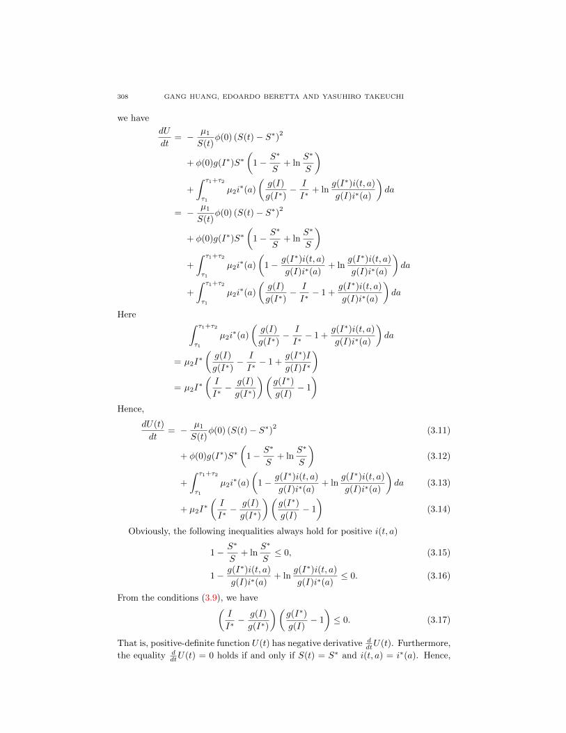
dU(t)

dt= − µ1

S(t)φ(0) (S(t)− S∗)2

(3.11)

+ φ(0)g(I∗)S∗(

1− S∗

S+ ln

S∗

S

)(3.12)

+

∫ τ1+τ2

τ1

µ2i∗(a)

(1− g(I∗)i(t, a)

g(I)i∗(a)+ ln

g(I∗)i(t, a)

g(I)i∗(a)

)da (3.13)

+ µ2I∗(I

I∗− g(I)

g(I∗)

)(g(I∗)

g(I)− 1

)(3.14)

Obviously, the following inequalities always hold for positive i(t, a)

1− S∗

S+ ln

S∗

S≤ 0, (3.15)

1− g(I∗)i(t, a)

g(I)i∗(a)+ ln

g(I∗)i(t, a)

g(I)i∗(a)≤ 0. (3.16)

From the conditions (3.9), we have(I

I∗− g(I)

g(I∗)

)(g(I∗)

g(I)− 1

)≤ 0. (3.17)

That is, positive-definite function U(t) has negative derivative ddtU(t). Furthermore,

the equality ddtU(t) = 0 holds if and only if S(t) = S∗ and i(t, a) = i∗(a). Hence,

GLOBAL STABILITY FOR EPIDEMIC MODEL 309

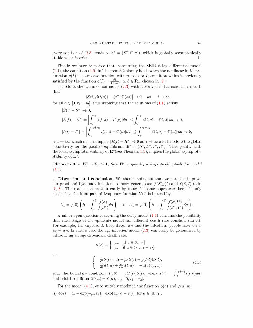
every solution of (2.3) tends to E∗ = (S∗, i∗(a)), which is globally asymptoticallystable when it exists.

Finally we have to notice that, concerning the SEIR delay differential model(1.1), the condition (3.9) in Theorem 3.2 simply holds when the nonlinear incidencefunction g(I) is a concave function with respect to I, condition which is obviously

satisfied by the function g(I) = βI1+αI , α, β ∈ R+ chosen in [2].

Therefore, the age-infection model (2.3) with any given initial condition is suchthat ∣∣(S(t), i(t, a))− (S∗, i∗(a))

∣∣→ 0 as t→∞for all a ∈ [0, τ1 + τ2], thus implying that the solutions of (1.1) satisfy

|S(t)− S∗| → 0,

|E(t)− E∗| =∣∣∣∣∫ τ1

0

[i(t, a)− i∗(a)]da

∣∣∣∣ ≤ ∫ τ1

0

|i(t, a)− i∗(a)| da→ 0,

|I(t)− I∗| =∣∣∣∣∫ τ1+τ2

τ1

[i(t, a)− i∗(a)]da

∣∣∣∣ ≤ ∫ τ1+τ2

τ1

|i(t, a)− i∗(a)| da→ 0,

as t→∞, which in turn implies |R(t)−R∗| → 0 as t→∞ and therefore the globalattractivity for the positive equilibrium E∗ = (S∗, E∗, I∗, R∗). This, jointly withthe local asymptotic stability of E∗(see Theorem 1.5), implies the global asymptoticstability of E∗.

Theorem 3.3. When R0 > 1, then E∗ is globally asymptotically stable for model(1.1).

4. Discussion and conclusion. We should point out that we can also improveour proof and Lyapunov functions to more general case f(S)g(I) and f(S, I) as in[7, 8]. The reader can prove it easily by using the same approaches here. It onlyneeds that the front part of Lyapunov function U(t) is instead by

U1 = ϕ(0)

(S −

∫ S

0

f(σ)

f(S∗)dσ

)or U1 = ϕ(0)

(S −

∫ S

0

f(σ, I∗)

f(S∗, I∗)dσ

).

A minor open question concerning the delay model (1.1) concerns the possibilitythat each stage of the epidemic model has different death rate constant (d.r.c.).For example, the exposed E have d.r.c. µE and the infectious people have d.r.c.µI 6= µE . In such a case the age-infection model (2.3) can easily be generalized byintroducing an age dependent death rate:

µ(a) =

{µE if a ∈ (0, τ1]µI if a ∈ (τ1, τ1 + τ2],

i.e. {ddtS(t) = Λ− µ1S(t)− g(I(t))S(t),∂∂t i(t, a) + ∂

∂a i(t, a) = −µ(a)i(t, a),(4.1)

with the boundary condition i(t, 0) = g(I(t))S(t), where I(t) =∫ τ1+τ2τ1

i(t, a)da,

and initial condition i(0, a) = ψ(a), a ∈ [0, τ1 + τ2].

For the model (4.1), once suitably modified the function φ(a) and ϕ(a) as

(i) φ(a) = (1− exp(−µIτ2)) · exp(µE(a− τ1)), for a ∈ (0, τ1],

310 GANG HUANG, EDOARDO BERETTA AND YASUHIRO TAKEUCHI

(ii) ϕ(a) =∫ τ1+τ2a

µI exp(µI(a− θ))dθ, for a ∈ [τ1, τ1 + τ2],

the proofs of the global asymptotic stability of the disease-free equilibria E0 whenR0 ≤ 1 and of the endemic equilibrium E∗ when R0 > 1 can be performed with thesame structure of the Lyapunov functions and by using the same technical detailsas in Theorems 3.1 and 3.2 respectively. It is to be noticed that in this case thebasic reproduction number R0 becomes

R0 =φ(0)S0

µIg′(0),

where S0 = Λ/µ1, and the endemic equilibrium component i∗(a) becomes

i∗(a) =

{g(I∗)S∗e−µEa for a ∈ (0, τ1],g(I∗)S∗e−µIa for a ∈ (τ1, τ1 + τ2].

The approach by the infection-age model followed in this paper to study theglobal stability properties for an SEIR model with two delays, of course, also appliesto the delayed SIR model. For example, Xu and Du in [22] considered a delayed SIRepidemic model with constant infectious period. That model they considered is aspecial case of model (1.1) where τ1 = 0. The global stability of endemic equilibriumwas left as an open question. Here we also solved this problem. Further, comparingwith the general age-infection model in [15], the mortality rate of i(t, a) in thisnonlinear age-infection model is assumed to be constant µ2. Our results generalizepartly the results in Magal et. al., [15] and McCluskey [16] to nonlinear incidencerate.

On the other hand, in this paper we establish the global stability for the age-infection epidemic model with nonlinear incidence rate. Actually, we find that mostepidemiological models with or without time delay can be regarded as specific casesof age-infection model (2.3).

(I) When τ1 = 0 and τ2 =∞, we have I(t) =∫∞

0i(t, a)da, and

d

dtI(t) =

d

dt

∫ ∞0

i(t, a)da = i(t, 0)− i(t,∞)− µ2I(t)

= g(I(t))S(t)− µ2I(t),

since g(I(t))S(t) is bounded as t→∞. Hence, age-infection model (2.3) is equiva-lent to the following ordinary differential equation SIR model,

S′(t) = Λ− µ1S(t)− g(I(t))S(t),

I ′(t) = g(I(t))S(t)− µ2I(t), (4.2)

R′(t) = γI(t)− µ3R(t).

The stability of the above SIR model with nonlinear incidence rate has been estab-lished by Korobeinikov et al. [10, 11, 12].

(II) When τ1 is a positive constant and τ2 = ∞ , we have E(t) =∫ τ1

0i(t, a)da,

I(t) =∫∞τ1i(t, a)da, and

d

dtI(t) = exp(−µ2τ1)g(I(t− τ1))S(t− τ1)− µ2I(t).

GLOBAL STABILITY FOR EPIDEMIC MODEL 311

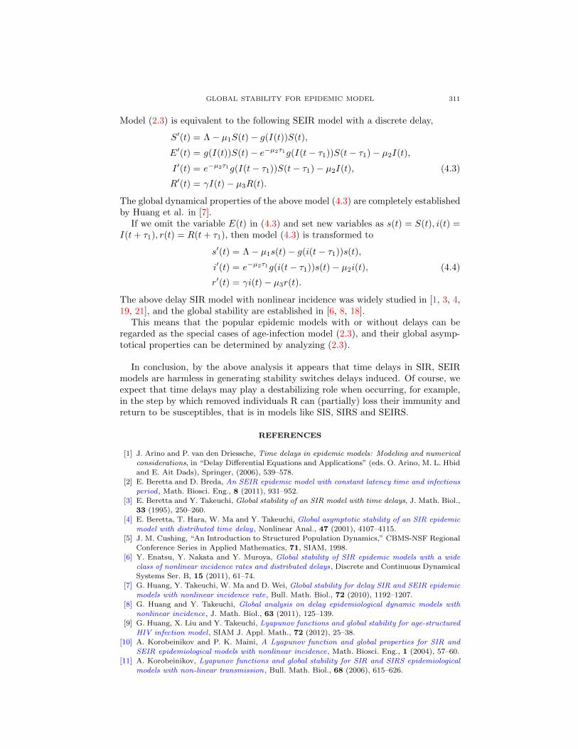
Model (2.3) is equivalent to the following SEIR model with a discrete delay,

S′(t) = Λ− µ1S(t)− g(I(t))S(t),

E′(t) = g(I(t))S(t)− e−µ2τ1g(I(t− τ1))S(t− τ1)− µ2I(t),

I ′(t) = e−µ2τ1g(I(t− τ1))S(t− τ1)− µ2I(t), (4.3)

R′(t) = γI(t)− µ3R(t).

The global dynamical properties of the above model (4.3) are completely establishedby Huang et al. in [7].

If we omit the variable E(t) in (4.3) and set new variables as s(t) = S(t), i(t) =I(t+ τ1), r(t) = R(t+ τ1), then model (4.3) is transformed to

s′(t) = Λ− µ1s(t)− g(i(t− τ1))s(t),

i′(t) = e−µ2τ1g(i(t− τ1))s(t)− µ2i(t), (4.4)

r′(t) = γi(t)− µ3r(t).

The above delay SIR model with nonlinear incidence was widely studied in [1, 3, 4,19, 21], and the global stability are established in [6, 8, 18].

This means that the popular epidemic models with or without delays can beregarded as the special cases of age-infection model (2.3), and their global asymp-totical properties can be determined by analyzing (2.3).

In conclusion, by the above analysis it appears that time delays in SIR, SEIRmodels are harmless in generating stability switches delays induced. Of course, weexpect that time delays may play a destabilizing role when occurring, for example,in the step by which removed individuals R can (partially) loss their immunity andreturn to be susceptibles, that is in models like SIS, SIRS and SEIRS.

REFERENCES

[1] J. Arino and P. van den Driessche, Time delays in epidemic models: Modeling and numerical

considerations, in “Delay Differential Equations and Applications” (eds. O. Arino, M. L. Hbidand E. Ait Dads), Springer, (2006), 539–578.

[2] E. Beretta and D. Breda, An SEIR epidemic model with constant latency time and infectiousperiod , Math. Biosci. Eng., 8 (2011), 931–952.

[3] E. Beretta and Y. Takeuchi, Global stability of an SIR model with time delays, J. Math. Biol.,

33 (1995), 250–260.

[4] E. Beretta, T. Hara, W. Ma and Y. Takeuchi, Global asymptotic stability of an SIR epidemicmodel with distributed time delay, Nonlinear Anal., 47 (2001), 4107–4115.

[5] J. M. Cushing, “An Introduction to Structured Population Dynamics,” CBMS-NSF RegionalConference Series in Applied Mathematics, 71, SIAM, 1998.

[6] Y. Enatsu, Y. Nakata and Y. Muroya, Global stability of SIR epidemic models with a wide

class of nonlinear incidence rates and distributed delays, Discrete and Continuous DynamicalSystems Ser. B, 15 (2011), 61–74.

[7] G. Huang, Y. Takeuchi, W. Ma and D. Wei, Global stability for delay SIR and SEIR epidemic

models with nonlinear incidence rate, Bull. Math. Biol., 72 (2010), 1192–1207.[8] G. Huang and Y. Takeuchi, Global analysis on delay epidemiological dynamic models with

nonlinear incidence, J. Math. Biol., 63 (2011), 125–139.

[9] G. Huang, X. Liu and Y. Takeuchi, Lyapunov functions and global stability for age-structuredHIV infection model , SIAM J. Appl. Math., 72 (2012), 25–38.

[10] A. Korobeinikov and P. K. Maini, A Lyapunov function and global properties for SIR and

SEIR epidemiological models with nonlinear incidence, Math. Biosci. Eng., 1 (2004), 57–60.[11] A. Korobeinikov, Lyapunov functions and global stability for SIR and SIRS epidemiological

models with non-linear transmission, Bull. Math. Biol., 68 (2006), 615–626.

312 GANG HUANG, EDOARDO BERETTA AND YASUHIRO TAKEUCHI

[12] A. Korobeinikov, Global properties of infectious disease models with nonlinear incidence,Bull. Math. Biol., 69 (2007), 1871–1889.

[13] M. Iannelli, “Mathematical Theory of Age-Structured Population Dynamics,” Applied Math-

ematical Monographs, 7, Consiglio Nazionale delle Ricerche, CNR, Giardini Editori e Stam-patori in Pisa, Aprile, 1995.

[14] A. V. Melnik and A. Korobeinikov, Lyapunov functions and global stability for SIR and SEIRmodels with age-dependent susceptibility, (2011), preprint.

[15] P. Magal, C. C. McCluskey and G. Webb, Lyapunov functional and global asymptotic stability

for an infection-age model , Appl. Anal., 89 (2010), 1109–1140.[16] C. C. McCluskey, Delay versus age-of-infection–global stability, Appl. Math. Comput., 217

(2010), 3046–3049.

[17] C. C. McCluskey, Global stability for an SIR epidemic model with delay and nonlinear inci-dence, Nonlinear Anal. RWA, 11 (2010), 3106–3109.

[18] C. C. McCluskey, Global stability of an SIR epidemic model with delay and general nonlinear

incidence, Math. Biosci. Eng., 7 (2010), 837–850.[19] P. van den Driessche, Some epidemiological models with delays, in “Differential Equations

and Applications to Biology and To Industry” (eds. M. Martell, K. Cooke, E. Cumberbatch,

R. Tang and H. Thieme), World Scientific, (1994), 507–520.[20] G. F. Webb, “Theory of Nonlinear Age-Dependent Population Dynamics,” Marcel Dekker,

New York, 1985.[21] R. Xu and Z. Ma, Global stability of a SIR epidemic model with nonlinear incidence rate and

time delay, Nonlinear Anal. RWA, 10 (2009), 3175–3189.

[22] R. Xu and Y. Du, A delayed SIR epidemic model with saturation incidence and a constantinfectious period , J. Appl. Math. Comput., 35 (2011), 229–250.

Received August 16, 2011; Accepted December 29, 2011.

E-mail address: huanggang10@yahoo.cn

E-mail address: edoardo.beretta@uniurb.it

E-mail address: takeuchi@sys.eng.shizuoka.ac.jp