New procedure to determine steel mechanical parameters from the spherical indentation technique

New procedure to determine steel mechanical parametersfrom the spherical indentation technique

A. Nayebi, R. El Abdi *, O. Bartier, G. Mauvoisin

Laboratoire de Recherche en M�eecanique Appliqu�eee de l’Universit�ee de Rennes, I.U.T. de Rennes. 3, rue du Clos Courtel – B.P. 90422,35704 Rennes cedex 7, France

Received 2 April 2001; received in revised form 2 January 2002

Abstract

A new numerical and experimental approach for determining mechanical properties of steels is presented. This

method uses the instrumented spherical-indentation technique. A relationship between applied load, indenter dis-

placement, flow stress and strain hardening exponent of steels, is given. This method is based on the minimisation of

error between the experimental curve (applied load–indenter displacement curve) and the theoretical curve which is a

function of the mechanical properties of studied materials. Comparison between the results obtained by the proposed

method and experimental tensile tests, confirms the interest of the proposed method. � 2002 Elsevier Science Ltd. All

rights reserved.

Keywords: Indentation method; Finite-element modelling; Hardness; Strain hardening exponent; Yield stress

1. Introduction

Indentation experiments have been performedfor nearly one hundred years for measuring thehardness of materials. Long time ago, as early asthe 19th century, the work of Hertz on rubbersappeared. Indentation of rubber can be interpretedin terms of elastic parameters using Hertz’s theory(1882) for a spherical indenter, or using Sneddon’sequations for a conical indenter (Sneddon, 1965).

For metals in a plastic state, Tabor (1951) wasthe first to point out the relation between Vickers

(HV) or Brinell (HB) hardness and yield stress ry,namely

HV � 3ry and HB � 2:8ry: ð1Þ

This experimental observation was backed up bytheoretical analyses of plastic flow, based on theSlip Line Fields method for spherical indenters(Ishlinsky, 1944), for a cone (Lockett, 1963) andthe generalisation to the Vickers pyramid byHaddow and Johnson (1961). These studies con-firmed the value of HV � 3ry for blunt indenters,and also derived solutions for sharper indenters.

Purely plastic analyses proved insufficient forhard metals where elasticity cannot be neglected.Following observations by Marsh (1964), ananalogy with the classical problem of the growth

Mechanics of Materials 34 (2002) 243–254

www.elsevier.com/locate/mechmat

*Corresponding author. Fax: +33-223-234101.

E-mail address: [email protected] (R. El Abdi).

0167-6636/02/$ - see front matter � 2002 Elsevier Science Ltd. All rights reserved.

PII: S0167-6636 (02 )00113-8

of a cavity in an infinite elastoplastic medium wasused to determine the relationship between thehardness number (or average indentation pressure)and parameters mixing geometry with elastic andplastic properties of the indented material (John-son, 1970; Edlinger et al., 1993; Giannakopoulosand Suresh, 1999; Venkatesh et al., 2000).

The traditional method of determining the yieldstress and the strain hardening exponent of a steelis the tensile test (or compression test) which re-quires the machining of samples which are, mostof the time, cylindrical. On the other hand, thespherical-indentation method can be used for de-termining material stress–strain behaviour in anon-destructive and localised fashion. Moreover,it does not need precise sample machining (Fieldand Swain, 1995).

The standard indentation measurement consistsof pushing an indenter into the sample underprecise load control. The indenter is inserted tosome specified depth and then extracted, giving theloading force over the whole depth range.

Recent years have seen increasing interest inindentation because of the significant improve-ment in the indentation equipment and the needfor measuring the mechanical properties of mate-rials on small scales. From the load–displacementcurve of an indenter during indentation, thehardness and Young’s modulus (for example) maybe obtained from the peak load and the initialslope of the unloading curves. The initial rate ofchange following the decrease in force (i.e., theslope) is defined as the sample stiffness.

Mechanical analysis requires formulation of thesharp indentation problem which is inevitablythree-dimensional and at first glance seems quiteimpossible to solve, mainly because of materialand geometric non-linearities, various dissipativemechanisms such as plasticity, phase transforma-tion, micro-cracking and the presence of residualstresses. The properties of the indenter, such as itssharpness, are also very important to the analysis.The combination of all these effects makes theproblem difficult to address analytically, and forthis reason it was left unsolved in the past. Today’scomputational capacity is, however, sufficient for adetailed investigation of the important features ofsharp indentation tests. Concerning the problemsfor which the indenter has an axisymmetric form(cones, spheres, etc.), a model using two dimen-sional finite elements (2D) often remains sufficient.

The problem of stress–strain curve determina-tion from indentation tests has been studied in thepast. The use of the stress–strain curve must leadto information about mechanical characteristicparameters.

Tabor (1951) has shown a direct relation be-tween indentation diameter and average appliedstrain, average pressure and corresponding stress.Field and Swain (1995) have used micro-sphericalindentation for determining a small volume ofmaterial mechanical properties. They have used astepwise indentation with a partial unloadingtechnique for separating elastic and plastic com-ponents of indentation at each step. Later, Jaya-raman et al. (1998), using different angle conical

Nomenclature

D diameter of balla contact radiusd indenter displacementdr residual depth of penetrationdmax maximum penetration depthr stressry yield stressm Poisson ratioE Young’s modulus

n strain hardening exponentepl plastic straineel elastic strainPav average contact pressureF applied loadFmax maximum applied loadS projected contact areaHV Vickers Hardnessq; h; z cylindrical co-ordinates

244 A. Nayebi et al. / Mechanics of Materials 34 (2002) 243–254

indenters, gave a method for determining the non-linear part of stress–strain curve. Taljat et al.(1998) used spherical indentation for determiningin another way the stress–strain curve. They havedetermined the relations for maximum and mini-mum applied strain and relating stresses, functionof contact diameter, indenter diameter and hard-ening exponent, but they have not given an exactmethod for determining the hardening exponent.Huber and Tsakmakis (1999a,b) have used aneural network and cyclic indentation for deter-mining the stress–strain curve. Bouzakis andVidakis (1999) have given a new procedure whichuses finite element simulation of successive ballindentation with increasing load. These methodsare usually difficult and time consuming, for ex-ample Huber’s method needs cyclic loading andBouzakis’ method needs a finite element simula-tion and measurement of imprint profile for everystress–strain curve point. Giannakopoulos andSuresh (1999) have used two parts of the loadingand unloading Vickers indentation curve for yieldstress and hardening exponent determination.They determine yield stress and stress at 0.29plastic strain so the hardening exponent can bedetermined from these values. But in another pa-per (Venkatesh et al., 2000), the authors specifiedthat their approach cannot distinguish two differ-ent materials which have the same yield stress ry

and the same r0:29 stress obtained for a plasticstrain equal to 0.29. The use of a Vickers indenterleads to the load–displacement F ¼ ad2 relationwhich is based on the determination of only oneparameter a and cannot lead to the uniqueness.This was shown by Cheng and Cheng (1999).

The aim of this work is to present a new pro-cedure which leads to determining the yield stressand the strain hardening exponent of steels usingan instrumented indentation technique and a the-oretical curve.

The experimental indentation test leads to ob-taining the load–displacement curve.

The theoretical curve is a relationship betweenapplied load, indenter displacement, yield stress ry

and the strain hardening exponent n of steels,which was determined by numerical simulations.

The procedure is based on the error minimisa-tion between the experimental (applied load–ind-

enter displacement curve) and the theoreticalcurves. This optimisation leads to having ry and n.

Several cylindrical samples from different steeltypes, are submitted to a tensile test and the ex-perimental values were compared with those nu-merically obtained from the proposed method.

Finally, we give a method which leads to ob-taining the Vickers hardness from knowing ry andn. This hardness value is compared to the oneobtained from the classical Vickers indentationtest.

2. Experimental procedure

2.1. Tensile test procedure

The tensile test has been used to have experi-mental comparison values. Tensile tests have beencarried out in a Lloyd LR30K machine. The ad-vance speed pertinent to the tensile tests is 2 mm/min. Cylindrical specimens 6mm in median diam-eter, having an effective length of 24 mm, wereused as tensile specimens (Fig. 1). Because of largestrains, an extensometer was used in the middle ofthe sample. A traditional system of acquisitionmakes it possible to record the tensile curve. Fig. 1gives the 100C6 steel stress–strain curve. Thistensile curve is fitted to Eq. (2), and the best valuesof ry and n so obtained were listed in Table 1.

Eq. (2) represents the strain–stress curve of ametal:

r ¼ Ken ¼ enry=ðry=EÞn; ð2Þwhere e is the total strain (e ¼ epl þ eel), and n is thestrain hardening exponent.

n ¼ 0 indicates a perfectly plastic material.

Fig. 1. Tensile curve for the 100C6 steel.

A. Nayebi et al. / Mechanics of Materials 34 (2002) 243–254 245

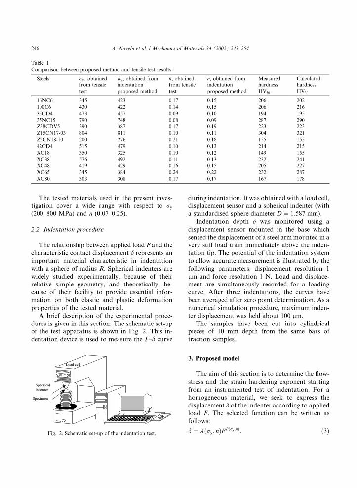
The tested materials used in the present inves-tigation cover a wide range with respect to ry

(200–800 MPa) and n (0.07–0.25).

2.2. Indentation procedure

The relationship between applied load F and thecharacteristic contact displacement d represents animportant material characteristic in indentationwith a sphere of radius R. Spherical indenters arewidely studied experimentally, because of theirrelative simple geometry, and theoretically, be-cause of their facility to provide essential infor-mation on both elastic and plastic deformationproperties of the tested material.

A brief description of the experimental proce-dures is given in this section. The schematic set-upof the test apparatus is shown in Fig. 2. This in-dentation device is used to measure the F–d curve

during indentation. It was obtained with a load cell,displacement sensor and a spherical indenter (witha standardised sphere diameter D ¼ 1:587 mm).

Indentation depth d was monitored using adisplacement sensor mounted in the base whichsensed the displacement of a steel armmounted in avery stiff load train immediately above the inden-tation tip. The potential of the indentation systemto allow accurate measurement is illustrated by thefollowing parameters: displacement resolution 1lm and force resolution 1 N. Load and displace-ment are simultaneously recorded for a loadingcurve. After three indentations, the curves havebeen averaged after zero point determination. As anumerical simulation procedure, maximum inden-ter displacement was held about 100 lm.

The samples have been cut into cylindricalpieces of 10 mm depth from the same bars oftraction samples.

3. Proposed model

The aim of this section is to determine the flow-stress and the strain hardening exponent startingfrom an instrumented test of indentation. For ahomogeneous material, we seek to express thedisplacement d of the indenter according to appliedload F. The selected function can be written asfollows:

d ¼ Aðry; nÞF Bðry;nÞ: ð3Þ

Table 1

Comparison between proposed method and tensile test results

Steels ry, obtained

from tensile

test

ry, obtained from

indentation

proposed method

n, obtained

from tensile

test

n, obtained from

indentation

proposed method

Measured

hardness

HV30

Calculated

hardness

HV30

16NC6 345 423 0.17 0.15 206 202

100C6 430 422 0.14 0.15 206 216

35CD4 473 457 0.09 0.10 194 195

35NC15 790 748 0.08 0.09 287 290

Z38CDV5 390 387 0.17 0.19 223 223

Z15CN17-03 804 811 0.10 0.11 304 321

Z2CN18-10 200 276 0.21 0.18 155 155

42CD4 515 479 0.10 0.13 214 215

XC18 350 325 0.10 0.12 149 155

XC38 576 492 0.11 0.13 232 241

XC48 419 429 0.16 0.15 205 227

XC65 345 384 0.24 0.22 232 287

XC80 303 308 0.17 0.17 167 178

Fig. 2. Schematic set-up of the indentation test.


Functions A and B depend on the yield stress ry

and the strain hardening exponent n, and are de-duced from the analysis of the results obtained byfinite elements simulations on a series of materials.

Simulation of the force–displacement relationfor the indentation of a half-space using a spheri-cal indenter with a high elastic modulus, was per-formed using the axisymmetric and large strainelastoplastic feature of the Castem 2000 finite el-ement code (Millard, 2000), with uniaxial stress–strain data as input. Materials with various yieldstresses and hardening components were studied.The quasi-static nature of the process allows usingthe static analysis performed by the programme.Underlying the approach in this code is the dis-cretization of the continuum involved. Also, animportant feature of this programme involves theability to model contact between the indenter andthe sample as a sliding interface. Initially, there iscontact at only one point between the indenter andthe sample. Progressively as the indenter pro-gresses, the programme automatically establishesthe junction between the contact surface nodes ofthe sample surface and those of the indenter.

An elastic sphere indenting an elastoplastic steelfor an axisymmetric half-space under normalcontact was considered and modelled using a fi-nite-element model in which the boundary condi-tions are given in Fig. 3; the boundary conditionsmay be expressed as follows:

rzðq; 0Þ ¼ 0 for jqj > a; ð4Þ

sqhðq; 0Þ ¼ 0 for jqj > a; ð5Þwhere a is the contact radius.

Far from the indentation zone, the displace-ments are cancelled:

u ¼ v ¼ 0 as q; z ! 1: ð6Þ

A finite element mesh of the half-space is given inFig. 4. The programme was used with 6316 ele-ments and 5986 nodes. A total of at least 30 ele-ments were allowed to come in contact with thesubstrate in order to provide sufficient resolutionin the computation of the field around the inden-ter. Other smoothness meshes were tested. Theconclusion was that the results were identical.

Table 2 gives several values of ry and n whichrepresent various studied materials.

For reducing numbers of simulations and pa-rameters, we have used an indenter with a constantdiameter as D ¼ 1:5875 mm and Young’s modulusas E ¼ 650 GPa. All the other steel parameters(Young’s modulus E ¼ 210 GPa, Poisson ratiom ¼ 0:3) remain constant.

The friction coefficient at the indenter–materialcontact was varied from 0.0 to 1.0. Various frictioncoefficients were used, and their influence on theF–d curve is negligible. Thus, for the studied ma-terials, it will be considered constant and equal to0.2 (Taljat et al., 1998).

For all homogeneous steels cited in Table 1,functions A and B have been determined as

B ¼ 1= ð0:151ry þ 0:609Þnþ 0:09ry þ 0:975� �

;

A ¼ ð3294þ 22170r0:8y Þe2:9nr0:323

y

h iB:

ð7ÞYield stress ry is in GPa.

For 35CD4 steel, Fig. 5 gives the load–dis-placement curve obtained from experimental test-ing and the proposed theoretical curve (3). Using

Fig. 3. Geometry and boundary conditions.


an optimisation procedure, we minimise the errorbetween the proposed theoretical curve and theexperimental indentation curve (F–d). This opti-misation yields parameters ry and n which makeerror minimisation. For 35CD4 steel, the errorminimisation leads to ry ¼ 457 MPa and to

n ¼ 0:10 whereas the values obtained from theexperimental tensile test are ry ¼ 473 MPa andn ¼ 0:09.

For several steels, ry and n values obtainedfrom the proposed method and tensile test arelisted in Table 1. The two methods lead to closeresults.

4. Hardness–flow stress relation

From ry and n values, we can have the hardnessvalues. A method for the determination of thehardness value is proposed.

4.1. Average contact pressure Pav

The spherical cavity expansion model expressesthe hardness value (average contact pressure) toelastic modulus ratio (Pav=E) as a function of theflow stress to elastic modulus ratio ðry=EÞ for veryhard or elastic materials. Thus, the linear hard-ness–flow stress correlation obtained from theSlip-Line Field theory can be rewritten in terms ofPav=E and ry=E. Due to the 1=E dependence inthese relations, the elastic modulus was used as thenormalising parameter. As a first step in develop-ing the hardness–flow stress correlation usingthe elastic modulus as the normalising parameter,the dependence of equivalent plastic strain epl on

Fig. 4. Finite-element meshing of half-space and zoom of the surface contact.

Table 2

Series of tested materials

ry (MPa) n n n n n

400 0.0 0.1 0.2 0.3 0.4

600 0.0 0.1 0.2 0.3 0.4

800 0.0 0.1 0.2 0.3 0.4

1000 0.0 0.1 0.2 0.3 0.4

1200 0.0 0.1 0.2 0.3 0.4

Fig. 5. Load–displacement curve for the 35CD4 steel.


the equivalent flow stress ry was given by thesimple Ramberg–Osgood equation:

epl ¼ Lðry=EÞN : ð8Þ

Any definition of the characteristic plastic strainshould be such that it is (i) dependent on the ge-ometry of the self-similar indenter, and (ii) inde-pendent of the depth of penetration (Jayaramanet al., 1998). For a given material, an experimen-tally determinable parameter that can satisfy boththese conditions is average pressure Pav. If thecharacteristic plastic strain epl is related to averagepressure Pav by a function similar to Eq. (8), wehave

epl ¼ L0ðPav=EÞN0: ð9Þ

Such a definition identifies the material being in-dented in terms of the new parameter L0 and N 0,while satisfying conditions (i) and (ii) mentionedabove. Thus, for a given indenter geometry, Eqs.(8) and (9) give a hardness–flow stress relation ofthe form:

Pav=E ¼ Cðry=EÞG; ð10Þ

where

C ¼ ðL=L0Þ1=N0and G ¼ N=N 0: ð11Þ

This theory connects Pav and ry through twoconstants C and G which depend on materialproperties and which are difficult to determine.This relation gives only the average contact pres-sure Pav and not the Vickers hardness. The fol-lowing paragraph presents a method for obtainingVickers hardness from ry and n.

4.2. Vickers hardness determination from mechan-ical properties

Fig. 6 is a schematic of the load–penetrationdepth (F–d) curve for a sharp indenter. Duringloading, the curve generally follows the power re-lation F ¼ W dm, where W and m depend on themechanical material parameters and on the ind-enter geometry.

The stress–strain curve of a metal can be char-acterised by a Hollomon-type Eq. (2).

The average contact pressure Pav is defined asthe ratio of the applied load F divided by theprojected contact area S. Finite-element simula-tion of elastoplastic indentation along with ex-periments (e.g., Giannakopoulos et al., 1994)provides the following results:

PavE� ¼ 0:27

E� r0:29

�þ ry

�1

�þ ln

E tanð22�Þ3ry

� ��;

ð12Þ

Fmax

d2max

¼ 7:143 r0:29

�þ ry

�� 1þ ln

E�

ry

� ��; ð13Þ

where 22� is the actual indentation angle ofthe Vickers indenter, Fmax is the maximum value ofthe applied load F and dmax is the maximum pen-etration depth. E� the effective modulus, is definedby

E� ¼ 1 m2

E

þ 1 m2ind

Eind

1

; ð14Þ

where E and m are Young’s modulus and Poissonratio, respectively, for the specimen and Eind andmind are the same parameters for the indenter. InEq. (12), r0:29 is the stress corresponding to thecharacteristic plastic strain of 0.29 for the indentedmaterial, deduced from Eq. (2):

Fig. 6. A schematic representation of load versus indenter

displacement data for an indentation experiment.


r0:29 ¼ K eplð0:29Þ�

þ eel�n: ð15Þ

By accounting for the effects of strain hardeningon pile-up and sinking down, and on the truecontact area, Giannakopoulos and Suresh (1999)proposes the following relation between the max-imum contact area Smax and the maximum pene-tration depth dmax:

Smax

d2max

¼ 9:96 12:64ð1 T Þ þ 105:42ð1 T Þ2

229:57ð1 T Þ3 þ 157:67ð1 T Þ4

with T ¼ PavE� : ð16Þ

Usually T is the experimentally measured stiffnessof the upper portion of the unloading data.

On the other hand, the effective elastic modulusE� of the indenter-specimen is defined as (Gian-nakopoulos and Suresh, 1999)

E� ¼ 1

c�ffiffiffiffiffiffiffiffiffiSmax

p dFdd

� �: ð17Þ

The constant c� ¼ 1:142 for the Vickers pyramidindenter, 1.167 for Berkovich indenter and 1.128for the circular conical indenter of any includedapex angle. dF =dd is the slope of the F–d curve ofthe initial stages of unloading from Fmax (Fig. 6).Thus, the use of Eq. (17) allows us to extract thevalue of dF =dd. Fig. 7 shows a cross section of anindentation and identifies the parameters used. Atany time during loading, the total indenter dis-placement d is written as

d ¼ dc þ ds; ð18Þ

where dc is the vertical distance along which con-tact is made and ds is the displacement of thesurface at the perimeter of contact. At peak load,the load and the displacement are Fmax: and dmax,respectively. Upon unloading, the elastic dis-placements are recovered, and when the indenter isfully withdrawn, the final depth of the residualhardness impression is dr.

The Sneddon’s force–displacement relationshipfor conical indenter yields (Oliver and Pharr,1992):

dr ¼ dmax 2Fmax

dF =ddð Þ : ð19Þ

For a pyramidal indenter with a half-angle of 68�and for a material under a load F, we can deter-mine the Vickers hardness HV as

HV ¼ 1:8544F

49d2r

: ð20Þ

In our case, the maximum applied load Fmax is 294N (HV30). From Eq. (13), we can deduce the valueof the maximum penetration depth dmax and cal-culating T ¼ Pav=E� from Eqs. (12) and (16) leadsto obtaining Smax. Knowing Smax and E�, Eq. (17)gives dF =dd, so from Eqs. (19) and (20) theVickers hardness can be calculated. Fig. 8 gives thehardness evolution in function of n and ry. Over-all, hardness evolution is an increasing function ofry, and for n ¼ 0 (perfectly plastic material)hardness is a linear function. Hardness is also an

Fig. 7. A schematic representation of a section through an in-

dentation.

Fig. 8. Hardness evolution versus the flow stress and the strain

hardening exponent.


increasing function of n, but this growth varieswith the ry value.

We have carried out the Vickers indentation teston many steels and Table 1 gives the comparison

between the experimental measured hardness val-ues and the calculated Vickers hardness obtainedfrom the presented method, in which n and ry

obtained from tensile tests are introduced. Fig. 9shows that the obtained results from the twomethods are similar.

5. Discussion

Several authors who use the indentation test todetermine the parameters of a material are satis-fied with an error of 20% (Venkatesh et al., 2000),moreover for brittle materials, the tensile test doesnot allow going beyond a few percent deforma-tion. However the indentation test makes it pos-sible to go beyond this limit. Steels presented inFig. 10 failed around 10% deformation under the

Fig. 9. Comparison between calculated and measured hardness

HV30.

(a)

(c) (d)

(b)

Fig. 10. Tensile and indentation curves (r ¼ Ken) for different steels.


tensile test. But the presented curves are extrapo-lated for a best comparison to the indentation re-sults. Using the behaviour law (2), we can have thestress evolution according to the strain. For foursteels (XC65, XC80, 100C6, 35CN15 steels), Figs.10(a)–(d) show that the results deduced by the twomethods lead to similar curves.

Most of the steels which we used obey theHollomon relation; since the experimental resultsare close to the values obtained from the suggestedmethod (see Table 1). On the other hand, Z2CN18-

10 steel presents a behaviour law different from thatof Hollomon. Therefore, for this material, it will benecessary to introduce its true behaviour law ob-tained from an experimental test. This true be-haviour law should be introduced in the proposedmodel.

Otherwise, Table 1 shows that the XC65 steel,which contains less carbon than XC80 steel, has ahardness (HV30 ¼ 232) higher than that of XC80steel (HV30 ¼ 167). Which goes against commonsense. A metallurgical analysis (Fig. 11) indicates

Fig. 11. Metallurgical analysis for different steels: (a) XC65 steel; (b) XC80 steel; (c) 100C6 steel; (d) 35CN15 steel.


that the XC65 steel used (Fig. 11(a)), has alamellar pearlitic structure and XC85 steel has aglobulized structure (Fig. 11(b)), thus less hard.100C6 steel is also globulized but has a highercarbon rate (1%) (Fig. 11(c)). Therefore it will beharder than XC80 steel (HV30(100C6)¼ 206).

The 35CN15 steel sample presents a bainiticstructure which appears fuzzy (Fig. 11(d)). We canhardly distinguish carbides aligned in needlepackages. It is a self-quenching steel, thus veryhard and its hardness is equal to 287.

In general, the hardness values obtainedfrom the Vickers indentation test and those ob-tained from the proposed method are similar(Table 1).

6. Conclusion

This paper presents a new procedure for deter-mining mechanical parameters of steel using theindentation test. Unlike the tensile test, the in-dentation test does not require the machining ofsamples. An experimental indentation test coupledwith a proposed method leads to the strain hard-ening exponent and the yield stress for steels. Onthe other hand, a theoretical approach is given(Eqs. (12)–(20)) and leads to the Vickers hardnessfrom the strain hardening exponent and the yieldstress.

The proposed model gives the indenter dis-placement evolution according to the loadingd ¼ Aðry; nÞF Bðry;nÞ. This model is based on aminimisation procedure of error between the pro-posed model and the finite element simulation re-sults. From the indentation displacement–loadcurve, the model yields the steel mechanical pa-rameters, ry and n.

The proposed method involves the followingsteps:

1. Experimentally determine the (F–d) curve dur-ing loading by a spherical indenter with radiusof a 1.5875 mm.

2. Use minimisation procedure between the (F–d)relation (3) and the experimental curve, wecan determine ry and n.

3. With the above theoretical framework (Eqs.(12)–(20)), the Vickers hardness can be calcu-lated.

References

Bouzakis, K.D., Vidakis, N., 1999. Superficial plastic response

determination of hard isotropic materials using ball inden-

tations and a FEM optimisation technique. Mater. Charact.

42 (1), 1–12.

Cheng, Y.T., Cheng, C.T., 1999. Can stress–strain relation-

ships be obtained from indentation curves using coni-

cal and pyramidal indenters? J. Mater. Res. 14, 3493–

3496.

Edlinger, M.L., Gratacos, P., Montmitonnet, P., Felder, E.,

1993. Finite element analysis of elastoplastic indentation

with a deformable indenter. Eur. J. Mech. A/Solids 12 (5),

679–698.

Field, J.S., Swain, M.V., 1995. Determining the mechani-

cal properties of small volumes of material from submicro-

meter spherical indentations. J. Mater. Res. 10 (1), 101–

112.

Giannakopoulos, A.E., Suresh, S., 1999. Determination of

elastoplastic properties by instrumented sharp indentation.

Scr. Mater. 40 (10), 1191–1198.

Giannakopoulos, A.E., Larsson, P.L., Vestergaard, R., 1994.

Analysis of Vickers indentation. Int. J. Solid Struct. 31 (19),

2679–2708.

Haddow, J.B., Johnson, W., 1961. Indentation with pyramids I:

theory. Int. J. Mech. Sci. 3, 229–238.

Hertz, H., 1882. €UUber die Ber€uuhrung festischer K€oorper. Z.

Reine und Angewande Math. 92, 156–171.

Huber, N., Tsakmakis, C., 1999a. Determination of constitu-

tive properties from spherical indentation data using

neural networks Part I: the case of pure kinematic harden-

ing in plasticity laws. J. Mech. Phys. Solids 47 (7), 1569–

1588.

Huber, N., Tsakmakis, C., 1999b. Determination of constit-

utive properties from spherical indentation data using

neural networks Part II: plasticity with nonlinear isotropic

and kinematic hardening. J. Mech. Phys. Solids 47 (7),

1589–1607.

Ishlinsky, A.J., 1944. Axisymmetric plastic flow in the Brinell

test. Prik. Math. Mekh. 8, 201–224 (in Russian).

Jayaraman, S., Hahn, G.T., Oliver, W.C., Rubin, C.A., Bastias,

P.C., 1998. Determination of monotonic stress–strain curve

of hard materials from ultra-low-load indentation tests. Int.

J. Solid Struct. 35 (5-6), 365–381.

Johnson, K.L., 1970. The correlation of indentation experi-

ments. J. Mech. Phys. Solids 18, 115–126.

Lockett, F.J., 1963. Indentation of a rigid plastic material by a

conical indenter. J. Mech. Phys. Solids 11, 345–355.

Marsh, D.M., 1964. Plastic flow in glass. Proc. R. Soc. A 279,

420–435.


Millard, A., 1992. Castem 2000. Guide du development.

Rapport D.E.M.T./92 300, C.E.A.

Oliver, W.O., Pharr, G.M., 1992. An improved technique for

determining hardness and elastic modulus using load and

displacement sensing indentation experiments. J. Mater.

Res. 7 (6), 1564–1583.

Sneddon, I.N., 1965. The relation between load and penetration

in the axisymmetric Boussineq problem for a punch of

arbitrary profile. Int. J. Eng. Sci. 3, 47–57.

Tabor, D., 1951. The Hardness of Metal. Clarendon Press,

Oxford.

Taljat, B., Zacharia, T., Kosel, F., 1998. New analytical

procedure to determine stress–strain curve from spherical in-

dentation data. Int. J. Solid Struct. 35 (33), 4411–4426.

Venkatesh, T.A., Vliet, K.J., Giannakopoulos, A.E., Suresh, S.,

2000. Determination of elasto-plastic properties by instru-

mented indentation: Guidelines for property extraction. Scr.

Mater. 42 (9), 833–836.


New procedure to determine steel mechanical parameters from the spherical indentation technique

Documents

Transcript of New procedure to determine steel mechanical parameters from the spherical indentation technique