Policy Research Working Paper 9597

New Evidence on Learning Trajectories in a Low-Income Setting

Natalie BauJishnu Das

Andres Yi Chang

Human Development Global Practice Office of the Chief EconomistMarch 2021

Pub

lic D

iscl

osur

e A

utho

rized

Pub

lic D

iscl

osur

e A

utho

rized

Pub

lic D

iscl

osur

e A

utho

rized

Pub

lic D

iscl

osur

e A

utho

rized

Produced by the Research Support Team

Abstract

The Policy Research Working Paper Series disseminates the findings of work in progress to encourage the exchange of ideas about development issues. An objective of the series is to get the findings out quickly, even if the presentations are less than fully polished. The papers carry the names of the authors and should be cited accordingly. The findings, interpretations, and conclusions expressed in this paper are entirely those of the authors. They do not necessarily represent the views of the International Bank for Reconstruction and Development/World Bank and its affiliated organizations, or those of the Executive Directors of the World Bank or the governments they represent.

Policy Research Working Paper 9597

Using a unique longitudinal data set collected from pri-mary school students in Pakistan, this paper documents four new facts about learning in low-income countries. First, children’s test scores increase by 1.19 standard devi-ation between Grades 3 and 6. Second, going to school is associated with greater learning. Children who drop out have the same test score gains prior to dropping out as those who do not but experience no improvements after dropping out. Third, there is significant variation in test score gains across students, but test scores converge over

the primary schooling years. Students with initially low test scores gain more than those with initially high scores, even after accounting for mean reversion. Fourth, conditional on past test scores, household characteristics explain little of the variation in learning. To reconcile the findings with the literature, the paper introduces the concept of “fragile learning,” where progression may be followed by stagnation or reversals. The implications of these results are discussed in the context of several ongoing debates in the literature on education in low- and middle-income countries.

This paper is a product of the Office of the Chief Economist, Human Development Global Practice. It is part of a larger effort by the World Bank to provide open access to its research and make a contribution to development policy discussions around the world. Policy Research Working Papers are also posted on the Web at http://www.worldbank.org/prwp. The authors may be contacted at ayichang@worldbank.org.

New Evidence on Learning Trajectories in a Low-Income Setting

Natalie Bau (UCLA), Jishnu Das (Georgetown University), and Andres Yi Chang (World Bank)1

JEL (I24,I25)

Keywords: learning, primary school, learning trajectories

1 We thank the RISE network for support and valuable comments on an earlier draft of this paper. We especially thank Michelle Kaffenberger, Karthik Muralidharan, Lant Pritchett, Zainab Qureshi, and Abhijeet Singh for their generous comments. Financial support for this research was made available through RISE grant PO13412. The findings, interpretations, and conclusions expressed in this paper are those of the authors and do not necessarily represent the views of the World Bank, its Executive Directors, or the governments they represent.

2

1. Introduction

What children learn during primary school and how learning varies by sex, parental background, and initial

test scores is of critical importance for education policy. Moreover, the process of learning and the

variation across subgroups may be very different in low-income countries (LICs) from high-income

countries. For instance, there is suggestive evidence that children with initially lower test scores learn less

in LICs due to “curricular mismatch” because curricular standards are set substantially higher than

children’s level of preparation (Pritchett and Beaty, 2015, Banerjee et al. 2016 and 2017, Kaffenberger

and Pritchett 2020a, Muralidharan, Singh and Ganimian 2019). Despite a shift in emphasis in the literature

on education in LICs from enrollment to learning and a large body of evaluative research on how to

improve test scores, there is currently little data on learning trajectories through primary school. We

address this vacuum, which is driven by the lack of large, longitudinal data sets of children’s test scores

during their primary schooling years, in this paper.

We use a rich longitudinal data set of children’s test scores over four years of primary schooling in

Pakistan, collected through the Learning and Educational Achievement in Punjab or LEAPS project, to

document four new facts about learning in low-income countries. First, we quantify how much children

learn in school. We find that an aggregate (mean) test-score measure of learning increased by 1.19 SD

between Grades 3 and 6. This implies that a high-performing child at the 75th percentile of the Grade 3

distribution “knew” as much as a low-performing child at the 25th percentile by Grade 6. Data from two

comparison groups – the Young Lives surveys of Peru, Vietnam, India, and Ethiopia, as well as

administrative data from Florida2 – show that, in all these settings, the rate of learning is similar

(approximately 1 SD over 4 years). Thus, gains across years, when measured relative to cross-sectional

variation, are similar in a highly disparate sample of countries.

Second, this learning does not solely reflect natural gains in reading, writing, and arithmetic skills as

children age. To distinguish “learning due to aging” from “learning due to schooling,” we tracked and

tested children who had dropped out between Grades 5 and 6, a transition that requires a change from

primary to middle school and may require more travel.3 In our data, the children who remained in school

between these grades gained 0.40 SD, while there was no statistically significant increase in test scores

2 Data for Florida were generously made available to us by David Figlio at Northwestern University. 3 LEAPS only tracked dropouts between Grades 5 and 6 and not in lower grades. Therefore, our results are limited to dropouts between these grades. The similarity of test score gains does not imply that rates of learning are identical, as these samples were administered different tests.

3

among dropouts. This could be because dropouts were negatively selected—perhaps they dropped out

because they were not learning. However, while dropouts reported slightly lower (but not statistically

significantly lower) test scores than children who continued in school, learning gains between Grades 3

and 5 were identical for dropouts compared to those who remained in school. This is consistent with the

‘parallel trends’ assumption required for this type of difference-in-difference estimate and suggests that

the gains we observe can be causally attributed to schooling itself.

Third, we find significant variation in how much children learn in our sample. The bottom decile of

“learners” in terms of test score gains (defined as the difference between final and initial test scores) lost

0.49 SD. The second decile gained 0.39 SD, and the top decile gained 2.77 SD over the four years of data.

The strongest determinant of how much a child learns between Grades 3 and 6 is her initial test score.

Children whose test scores were in the bottom 20% in Grade 3 learn significantly more, gaining 1.75 SD

between Grades 3 and 6, than children ranked in the top 20% (0.71 SD). Accounting for measurement

error reduces the relative gains of the lowest performers but does not reverse the pattern.

Fourth, conditional on past test scores, household characteristics explain little of the variation in test

scores between Grades 3 and 6. Regression estimates suggest that 56% of the variance in test score levels

in a given year is explained by lagged test scores, but including a full set of village and school fixed effects,

as well as parental and child characteristics, explains only another 6% of the variation. We focus on two

characteristics—gender and family wealth—in greater detail and show that our results are robust to

alternate methods of test scaling, an issue that has received considerable attention in recent work from

the United States.

These findings significantly broaden what we know about learning in low-income countries. Our first

finding – that students’ test scores increase by more than 1 SD on average over the course of 4 years of

primary school – contrasts with several studies arguing that many children progress very slowly through

schools with learning trajectories that “flatten” over the years (Beatty et al. 2018, Filmer et al. 2006,

Kaffenberger and Pritchett 2020b, Pritchett and Sandefur 2020). Yet, there are few school panels with

calibrated test questions that can be used to answer this basic question. In our novel panel, schooling

does appear to be associated with learning, at least on average. While comparing the magnitude of

learning gains measured with different tests across countries is difficult, we cannot reject that learning

gains are similar across a variety of settings.

4

Our second finding that students who attend school experience test score gains while dropouts do not

contrasts with past studies that have shown that programs incentivized to retain children in school and

increase enrollment do not improve test scores among treated cohorts (Hanushek et al. 2008; Behrman

et al. 2009; Filmer and Schady 2009; Zuilkowski et al. 2016; Nakajima et al. 2018).4 Importantly, our results

do not imply that test scores and dropout are not correlated. Even for the limited sample of children

moving between Grades 5 and 6, this correlation is positive.5 However, we are not aware of studies that

have tracked children for multiple years and compared the test-score trajectories of children who drop

out versus those who choose to continue. The specific result that there is no correlation between dropping

out and test score gains is new to the literature.

Our third finding – that test score gains are highly variant and largest among initially low performers –

relates to several studies that argue that many children, especially low performers, often start off learning

very little and that their learning trajectories flatten as they fall behind and stop learning at some point

during primary school (Beatty et al. 2018, Filmer et al. 2006, Kaffenberger and Pritchett 2020b,

Muralidharan, Singh and Ganimian 2019). We find the opposite pattern in our data. We discuss how the

disparity in findings across settings can be explained by subtleties in how learning is measured. Measuring

learning in terms of test score gains, as we do, would lead researchers to conclude that learning is highest

among the initially poorly-performing. Measures of learning that assume imperfect persistence of initial

test score levels with a common persistence parameter (e.g. Muralidharan, Singh and Ganimian, 2019)

lead to the opposite conclusion.

We further contribute to the literature by introducing the novel concept of “fragile learning” to reconcile

these findings. In our setting, as in most settings, test scores are not highly persistent across years. One

extreme consequence of low persistence is that learning trajectories are not monotonically increasing for

all children or all questions. In fact, a sizeable fraction of children experience test score losses every year.

Item-wise analysis shows that the fraction of children whose performance for specific questions features

gains followed by losses is as high as the fraction of children who are “robust learners,” or children whose

learning trajectories show either stability or monotonic increases every year. The difference between our

results and those of Muralidharan, Singh and Ganimian (2019) reflects how different specifications

4 These studies test a sample of children in treated and control areas, regardless of enrollment status. If children who are incentivized to remain in school also gain test scores, the studies should have found that children in treated areas have higher test scores than those in control areas. 5 Furthermore, completed schooling at age 22 is strongly correlated with test scores at age 12 in both the LEAPS and the Young Lives samples (Das, Singh and Yi Chang 2020).

5

account for fragile learning — unconditional test score levels converge, with low performers increasing

their test scores relatively more, but test score levels conditional on an imperfectly persistent baseline

test score do not. Understanding the causes and pedagogic basis of low persistence in low-income

countries is a fertile area for further investigation.

Our fourth finding – that wealth and gender explain little of the variation in current test scores conditional

on lagged test scores – is surprising, especially given a long history, dating back to the Coleman report, of

associating performance in tests with the home environment (Coleman 1966). However, it accords with

more recent results from high-income countries, where the difference between the correlates of levels

and gains has become more apparent with better data. A number of studies now show that family

background is strongly correlated with test score gains in the pre-school years but not necessarily

associated with gains (not levels) during the primary schooling years (Fryer and Levitt 2004, Reardon 2011

and 2013).

The remainder of the paper is organized as follows. We first describe the LEAPS data in Section 2 and

follow this with a description of the main patterns in Section 3. Section 3 also presents our regression

estimates and discusses how we address attrition and measurement error in the sample. Section 4

introduces the concept of fragile learning, and Section 5 concludes with a brief discussion. We emphasize

that this is a “first look” at the data, and there is considerable room for further research, both from an

educational and psychometric perspective.

2. Context and Data

2.1. Population and sampling

The LEAPS study was started in 2003 in the province of Punjab in Pakistan, which has an approximate

population of 70 million people and is the 12th largest schooling system in the world. A sample of 112

villages was drawn from three districts —Attock in the North, Faisalabad in the center, and Rahim Yar

Khan in the south— following an accepted stratification of the province along educational outcomes into

the better performing center and north and the poorly performing south. The sample was drawn from

villages with at least one private school, consistent with LEAP’s goal of understanding the role of private

schooling. For each of these districts, the list frame consisted of all villages that had at least one private

primary school within the relevant “choice set” for households in the village (schools in the village or

schools within a 15 minute boundary of the village in Attock and Faisalabad and a 30 minute boundary in

6

Rahim Yar Khan). In these villages, all schools in the choice-set were covered as part of the LEAPS project,

resulting in a total of 823 public and private schools in 2003. Between 2003 and 2006, we carried out tests

in 1,121 schools in 119 villages.6 The higher number of schools (1,121 versus 823) both reflects the exit

and entry of schools and our sampling strategy where we attempted to track and follow children at

whatever school they were in.

Andrabi et al. (2008) have compared the villages in the LEAPS sample to representative samples from

Punjab and show that these villages tend to be larger and wealthier, with greater access to infrastructure.

This follows from the restriction in the sample-frame that each village should have at least one private

school. Therefore, the learning patterns that we present here are not representative of either remote

rural villages or urban areas. Nevertheless, the range of household and school characteristics in the LEAPS

sample covers most villages in Punjab except for the poorest, since 60% of Punjab’s rural population lives

in a village with access to at least one private school (Andrabi et al. 2008).

Andrabi et al. (2008) also characterize the households and schools in these villages. Noteworthy features

of the sample in 2003, when the first survey was collected are: (a) 50% of household heads in the sample

reported no education at all; (b) about a quarter of household heads reported their primary occupation

as farming; and (c) the average household size was 7.5 members. Enrollment patterns reflect those in

many low-income countries, with 76% of boys between the ages of 5 and 15 enrolled in school in 2003

compared to 65% of girls, and a classic inverted U-shape in enrollment-age profiles, reflecting both late

entry into schooling and dropouts from age 11 onwards. Although we do not focus on learning differences

between private and public schools here (see Andrabi et al. 2020 for a causal analysis of private schooling

and test scores), we note that 70% of enrolled children were in public and 28% in private schools.

Enrollment in religious schools or madrassas was only 1%, reflecting nationwide enrollment patterns

(Andrabi et al. 2006).7

2.2. Data collection and samples

We use three data sets collected as part of the LEAPS surveys. These are (1) data on test scores, (2) data

on family characteristics, and (3) data collected from households. The first two data sets were collected

6 Since (a) schools open and close, and (b) in 2006, some children, who had moved on to middle school (Grade 6), were studying in schools outside the village, the total number of schools and villages is higher for the 4 years of testing. 7 The residual 1% corresponds to NGOs/community schools.

7

at schools and we refer to these samples as the “School Sample.” The sample in the third data set, which

was collected at households, is referred to as the “Household Sample.”

Test Scores in the School Sample: In each year between 2003 and 2006, the LEAPS study tested children

using tests designed in consultation with pedagogical and education experts in the subjects of English,

Urdu, and Mathematics. Tests were administered by the LEAPS team and were then recovered at the end

of the test, minimizing the possibility of manipulation or cheating. The norm-referenced tests covered a

wide range of concepts and capabilities in order to track how children learned over time. See Andrabi et

al. (2002) for a detailed description of the test. The tests were first administered in 2003 to children in

Grade 3 and then again in 2004, 2005, and 2006, as the majority of the children transitioned to Grades 5

and 6.8 New children found in the appropriate grade each year were also tested at the school. Each test

retained a rotating core of “linking items,” so that some questions were repeated from year to year. These

linking items allow us to calibrate all the tests on a common scale, following established methods in the

literature on Item Response Theory (Hambleton and Swaminathan 2013).

Tracking children over time for test data was challenging, especially as children do not have methods of

identification and switch schools over the multiple years of the survey. Every year, the LEAPS team

conducted an extensive tracking exercise, where we tried to ascertain the whereabouts of each child

enrolled in the relevant grade in the past year. Most children remained in the same school, but 5%-7%

switched schools. Sending schools had no information on whether these children had dropped out, left

the village, or were enrolled elsewhere, and teams spent several weeks trying to track the location of

these children.9 We will further discuss below how this affects the data.

Family Characteristics Data for the School Sample: On the day of the test in 2003, we sampled 10 children

randomly from each class and completed a short questionnaire with these students on their family

background. In subsequent years, we continued to complete the questionnaire with these children and

additionally surveyed randomly selected children from the same classroom.

Household Sample: Our third data source comes from a concomitant household survey carried out among

1,875 households in 2003 in the same villages. The household survey was designed to complement the

8 Some children, who were held back or double promoted, were tested in their new grades. 9 In practice, since we were following all schools and children in the relevant grade, we were successful in tracking children even when they moved in most cases. However, some children had similar names or used variants of the same name (Mohammed Abdul Karim may be in School A in year 2003 but then may move to School B in year 2004 and be registered as Abdul Karim) leading to inevitable uncertainty in these limited cases.

8

school survey and oversampled households with children between the ages of 9 and 11. In cases where

such a child was located in the household and was enrolled in the school, we have the test score of the

child and parental background variables that have been collected by the surveyors from the parents

themselves. Furthermore, in 2006, we were worried about extensive missing test scores as children

transitioned from primary to middle school. Therefore, to retain one consistent panel, we also tested

children who had been part of the school test-score panel during home visits. As we will discuss in more

detail, the household sample allows us to (1) assess how sensitive our results are to attrition and (2)

compare the learning trajectories of students who drop out and remain in school.

2.3. Measurement

In this subsection, we describe the two important components of our strategy to measure students’

learning. We first discuss the measurement of test scores with an item response model, and then describe

how we translate these test scores into our key measure of learning throughout the paper.

Test Score Measurement: In the Item Response Model, the likelihood of answering a question correctly is

determined by the ability of the child, labeled θ, and item parameters, labeled a, b, and c for difficulty (a),

discrimination (b), and a guessing parameter (c).10 If there are N children and M questions, then N + 3M

parameters are estimated through the IRT method, one θ for each child, and 3 parameters for each of the

M questions. For each item, the estimation produces an “Item Characteristic Curve” that provides, for

each θ, the likelihood that a question is answered correctly. The item characteristic curve is given by the

3-parameter logistic:

𝑃𝑃𝑗𝑗(𝜃𝜃) = 𝑐𝑐𝑗𝑗 + (1 − 𝑐𝑐𝑗𝑗)1

1 + exp {−𝑎𝑎𝑗𝑗�𝜃𝜃 − 𝑏𝑏𝑗𝑗�}

where 𝑐𝑐𝑗𝑗 is defined as the guessing parameter, since it’s the probability of getting the question right

through pure guessing; 𝑏𝑏𝑗𝑗 ≡ 𝜃𝜃∗|𝑃𝑃𝑗𝑗(𝜃𝜃∗) = 1+𝑐𝑐𝑗𝑗2

and is the difficulty parameter, which is the ability level at

which the child will answer the question correctly half the time (adjusted for guessing), and 𝑎𝑎𝑗𝑗 ∝𝜕𝜕𝑃𝑃𝑗𝑗(𝜃𝜃)𝜕𝜕𝜃𝜃

at

𝜃𝜃 = 𝑏𝑏𝑗𝑗, is the discrimination parameter, which specifies the steepness of the item characteristic curve at

the point that the ability of the child is equal to the difficulty of the question (𝑏𝑏𝑗𝑗).

10 Maximum likelihood estimates (MLE) of the underlying latent trait θ are used throughout this paper.

9

The joint estimation of these parameters follows the standard procedure in IRT using the IRT command,

OpenIRT, developed by Zajonc for STATA and discussed in Das and Zajonc (2008). In order to maximize

efficiency, we use all the data available by pooling test score data from 2003 to 2006 to jointly estimate

θ and the item parameters.11 An observation is at the child-year level, so test score gains are given by the

difference in θ for any child across two (or more) years. Even though the test can change in each year, the

exercise requires that across any two years, there are some common questions that can be used to “link”

items. Item parameters for these questions are assumed to be time invariant, allowing us to identify

parameters for other questions that are not common across years and place every θ on a common scale.

We describe how we assess item-invariance below. As θ can only be identified up to an arbitrary scale and

origin, we follow the convention that θ is drawn from a distribution with mean 0 and SD (approximately)

equal to 1 across the entirety of the sample.12

Measuring Learning: With the test score measures in hand, we identify the key object of interest in this

paper – learning gains. Our measure of a student 𝑖𝑖’s learning gain from period 𝑡𝑡0 to period T, which we

also refer to as the student’s test score trajectory, is given by 𝑦𝑦𝑖𝑖𝑖𝑖 − 𝑦𝑦𝑖𝑖,𝑡𝑡0. In the literature (see, for

example, Muralidharan, Singh and Ganimian 2019), annual learning is sometimes alternatively measured

with a value-added specification 𝑦𝑦𝑖𝑖𝑖𝑖 − 𝛽𝛽𝑦𝑦𝑖𝑖,𝑖𝑖−1. In this specification, 𝛽𝛽, identified from the data, captures

the imperfect persistence of test scores over time resulting from both measurement error and forgetting.

For much of this paper, we focus on the test score trajectory specification, since it exactly captures how

much a student’s level of knowledge (as proxied by her test score) increased over time. In Section 4, in

our discussion of fragile learning, we further compare these measures and point out areas where these

measures can lead to different conclusions.

2.4. Threats to the validity of the measures

Validation of the IRT Model in the LEAPs Data: The IRT model’s linking procedure assumes that test

parameters are invariant over time so that the increased likelihood of answering a particular question in

a particular year is fully determined by a change in the child’s θ. This is an assumption about the stability

of the item characteristic curve and assumes that, as children progress, they move along the estimated

curve, while the curve itself does not change. It is similar to the assumption of “no differential item

11 Although other cohorts were tracked over the years, IRT parameters are estimated using the 4 rounds of LEAPS test score data collected for the cohort of children in Grade 3 in 2003. 12 The model assumes a true distribution of θ with mean 0 and a SD of 1 in the presence of infinite data. In practice, the finite nature of our sample yields a distribution very close to the desired one but with minor deviations.

10

functioning” for horizontal test equating—for any two groups (say, by race), the likelihood of answering a

question correctly should depend only on underlying ability and not group membership.13

This is a strong assumption but one that can be empirically tested. Appendix Figure 1 shows the results

for an exercise where we first estimate item parameters from year 1 (2003) only, along with the

distribution of θ for the children in that sample. We then assume that the item parameters are fixed and

using the same parameters, we re-estimate new the new distribution of θ using their patterns of

responses for common items in year 4 (2006). We then plot (solid line) the expected patterns of responses

for each θ (the “item characteristic curve”) and the actual patterns of responses against θ. If the expected

and actual patterns of responses match, this implies that children are moving along a fixed item

characteristic curve and that the curve itself is not shifting across years.

For most items, we find a close match between the expected and observed response patterns. Many items

match almost exactly suggesting that vertical linking is possible in this setting and for this test, but there

are also some notable departures. Observed response patterns for Urdu Item 23, for instance, are far

above the expected response patterns with fixed item parameters at θ above the mean. This particular

question asks children to select the correct antonym for the word “victory” among the options (a)

“success,” (b) “defeat,” and (c) “weapon.” Another example is English Item 22 (which asks children to fill

in the missing letters to complete the word “fruit” next to a picture of fruits). Here, the observed patterns

are worse than expected suggesting that similarly knowledgeable children find it harder to answer this

question correctly in higher grades. It could be, for instance, that the Grade 3 curriculum included the

word “fruit,” but the Grade 5 curriculum did not have this particular word.

We tested these departures using Chi-Squared tests and are unable to reject equality for 61 of 80 common

items across years 1 and 4. We have also recomputed test score gains after (a) dropping the questions

where vertical equating seems to fail; and (b) including all questions, but fixing item parameters for the

61 items where they appear to be invariant and leaving item parameters to be estimated for the other 19,

where vertical equating seems to fail (see Appendix Table 1). We observe no appreciable difference in the

patterns of test score gains. Based on these exercises, we are cautiously optimistic that vertical linking is

13 A specific example of a question with differential item functioning in Pakistan is asking children to translate numbers into words (for instance, 22 is “Twenty-Two”). In our pilot, we noticed that children in schools taught predominantly in Urdu, as opposed to English, found these questions to be harder. The reason is that in Urdu, every number between 1 and 100 is different, while in English, once you know the numbers 1 through 10 in words as well as 20 (twenty), 30 (thirty), etc., numbers like 44 are easier to translate into words. Therefore, conditional on knowledge, children taught in Urdu find these questions harder than those taught in English.

11

viable with these data. We emphasize however, that this is an area that requires further refinement and

investigation for this data set.

Attrition: Attrition is a common problem in the collection of school-based test score data in low-income

countries, where student absenteeism rates can range from 10% to 20% on any given day due to sickness

or other emergencies at home. In our data set, there are 16,428 unique children who appear 47,105 times

over the 4 years. Of these unique child-year observations, 51% correspond to observations in every year,

and 82% to observations in at least 3 years. To address attrition, we pursue two avenues. Appendix A

explores the underlying dynamics that could produce similar attrition patterns to those we observe in

Table 2. We conclude that attrition is primarily due to a combination of random absence and a small

degree of miscoding in child IDs; however, we cannot rule out some degree of selection as well. Therefore,

in Section 3, we will discuss the potential bias induced through attrition by comparing samples who are

more and less intensively tracked and conclude that it is small.

3. Results

Our main results section proceeds in four parts, with each part describing one of the new facts generated

by the LEAPS data. Many of our results can be presented through tables and figures of means, and this is

what we focus on, augmenting these results with regression estimates to provide standard errors and

show robustness to attrition, measurement error, and test-score scaling.

3.1. How much do children learn?

Using the unbalanced school sample, Table 1 shows what children learn during primary schooling, focusing

on specific items that were repeated in every year. When first tested in Grade 3, most children could

match simple words in English to pictures (such as “book”), add and subtract 2-digit numbers, and

recognize Urdu alphabets and how to combine them into simple words (Urdu 10). But they could not

construct simple sentences in English (such as “I play” or “The water is deep”), multiply or divide, or read

an Urdu passage.

Tested again at the beginning of Grade 6, there are improvements in every item, typically in the range of

a 15 to 30 percentage point greater likelihood of a correct answer. By this time, children were learning

how to spell simple words in English, add and subtract larger numbers, and perform simple multiplication.

Moreover, 51% of children can divide 384 by 6, and a small minority can convert word challenges into

12

Math or complete simple operations with fractions. For the vernacular, Urdu, it seems that learning has

progressed sufficiently to allow students to fill in grammatically correct missing portions in a paragraph.

IRT scaling allows us to combine these item-level responses into a single score, which we report in Table

3. Here, the scores are computed for all students, and items across all four years and vertically equated

using linking items as discussed previously. Table 3 shows that in Pakistan, between Grade 3 and the

beginning of Grade 6 (ages 9.7 to 12.8), children have gained 1.08 SD in Mathematics and 1.29 SD in Urdu

for a combined average increase of 1.19 SD across these two subjects.

Robustness to attrition. One important question is whether our estimated learning gains are biased due

to attrition (or accretion). To evaluate the scope for attrition to affect our results, Table 2 reports the

sample of children observed in each of the four years of testing in the school sample. We first show the

number of rounds children appeared in, followed by basic child characteristics (sex and age), the average

number of days absent in the last month (as reported by their teacher), family characteristics (parental

education and assets), and their average annual test scores gains in the years they were observed.

Although there are small differences in child and parental characteristics across samples, regardless of the

sample of tested children we focus on (those observed for 2, 3, or 4 years), the average of our key metric

of annual learning gains is approximately 0.39 SD. The stability of this value across rounds provides initial

evidence that estimates of learning gains are not highly sensitive to selective attrition.14

We can further verify the extent to which test score gains in the schooling panel are unbiased by

identifying a sample where the pattern of attrition is less severe. The intuition here is similar to the idea

of “intensive tracking” or “double sampling” in clinical data (Baker et al 1993). Specifically, if missingness

is selective, the means computed from samples with ‘more’ and ‘fewer’ missing observations will be

informative of the selection process. If children who are missing are highly selected, as missingness

declines, we would expect to see meaningful changes in the estimated average test score gains. Appendix

A presents a formal argument for this intuition.

Using the household sample, we are able to compare a more and less intensively tracked sample. We have

constructed the analog to Table 2 for the household sample in Appendix Table 3. Here, the number of

children on whom we have test scores is much smaller (1,052), but 72% of the unique child-year

14 An important caveat is that children who are only observed once are never included in our calculations of learning gains since they do not have lagged test scores. We further discuss this group and the implications for our estimates in Appendix A.

13

observations correspond to test scores observed in every year, and 92% correspond to test scores

observed in at least 3 of 4 years. Furthermore, test scores for students who are observed in all four years

in the household and school sample track each other closely, with gains from the first to the fourth round

of 1.13 SD for the school sample compared to 1.10 SD for the household sample (with yearly test score

gains of approximately 0.38 SD).15 This suggests that selection bias is unlikely to strongly affect the average

annual test gains estimates in our setting, as a substantial decline in attrition when we use the household

instead of the school sample does not alter our main conclusions.

How does learning in the LEAPS sample compare to other settings? Our only recourse for comparison to

other settings with similarly equated test scores is the Young Lives study, which tested children in Ethiopia,

India, Peru and Vietnam, and data from Florida, where analysis was provided to us by David Figlio using

administrative data from that state. This is far from an ideal comparison. LEAPS and Florida are school-

level panels that tracked children who were first observed in Grade 3, while data in the Young Lives

countries is collected at the household-level, and initial selection into the panel starts at age 8 rather than

when children are enrolled in a specific grade. Furthermore, there are differences in the samples, with

LEAPS testing children only in rural areas but in all schools and the Young Lives using a representative

sample of urban and rural children in each of their settings.

Surprisingly, despite these substantial differences, test score gains over equivalent ages follow a very

similar pattern, with increases of 1 to 1.27 SD in these other settings. The exceptions are language gains

in Peru, which are notably higher, and Mathematics gains in Ethiopia, which fall below the average.

Although the similarity in relative gains is striking, we stress that this tells us little about absolute learning

across countries. Whether these patterns reflect more or less learning depends on the cross-sectional

variation in the baseline grade’s test scores, as well as the comparability of test score gains across different

parts of the learning distribution within each country. This comparison is also fragile because, if test scores

are normally distributed, a 1 SD gain throughout the distribution should always imply that children at the

75th percentile in Grade 3 “know” almost the same as children at the 25th percentile in Grade 6. Although

this is indeed the case for Pakistan and Florida, it is generally not true in the Young Lives countries. In

India, Vietnam and Peru, children at the 25th percentile at age 12 know more than children at the 75th

percentile at age 8, while the opposite is true in Ethiopia. The non-normality of these data could reflect

15 Test scores in 2003 were -0.56 SD in the household sample compared to -0.55 SD in the school sample and are therefore also statistically indistinguishable.

14

that fact that children tested at the same age are in very different grades, further complicating cross-

country comparisons.

3.2. Are test score gains due to “learning by aging?”

A second important question is the extent to which this learning reflects natural progression in vocabulary

and Math skills due to “learning by aging” as opposed to “learning by schooling.” Figure 1 Panel A plots

test scores in every round for two groups of students in the (unbalanced) school survey. The red line shows

students who were observed in every year. It is worth highlighting that the test score gains experienced

by these students between 2003 and 2006 (of 1.16 SD) are almost identical to what we observe for the

full school sample (1.15 SD). The blue line shows test scores in every round for students who eventually

dropped-out in the transition from primary to middle school. The last score for this group therefore

reflects their scores when they were tested at home and had been out of school for one year. Figure 1

Panel B plots the yearly test score differences between these two groups with their respective 95%

confidence intervals.

Test score gains track each other very closely between 2003 and 2005. There is a small but imprecisely

estimated difference of 0.05SD to 0.09SD in test scores levels in favor of the children who continued, but

there are no differences in gains. However, immediately after children dropout, the test score differences

increase to 0.40 SD from 0.09 SD in the preceding year. The analog of this figure for the household panel

(Appendix Figure 2) shows similar patterns prior to dropout, but starker differences after dropping out, as

children who are no longer in school report lower test scores in the year after dropping out. This striking

finding suggests that children who drop out were learning no less than those who chose to continue. It is

also an indication that school continuation remains an important source of inequality. The children who

dropped out were more likely to come from less wealthy households with lower parental education (on a

standardized asset index, the children who dropped out were 0.32 SD below those who continued, 12%

of their mothers and 40% of their fathers had completed at least primary education compared to 24% of

mothers and 55% of fathers for those who continued).

Table 4 shows the regression equivalent to Figure 1 using the (unbalanced) school sample. We present

four specifications, which differ in how we treat persistence in learning and how we treat dropouts. First,

in columns 1 and 2, we present the association between dropping out and level test scores, either by

examining the impact of dropping out in Round 4 (Column 1) or by allowing dropouts to have different

test score gains in each year (Column 2), even before they dropout. Specifically, Column 1 estimates:

15

𝑦𝑦𝑖𝑖𝑡𝑡 = 𝛽𝛽0 + 𝛽𝛽1(𝑦𝑦𝑦𝑦𝑎𝑎𝑦𝑦 = 2004) + 𝛽𝛽2(𝑦𝑦𝑦𝑦𝑎𝑎𝑦𝑦 = 2005) + 𝛽𝛽3(𝑦𝑦𝑦𝑦𝑎𝑎𝑦𝑦 = 2006) + 𝛽𝛽4(𝐷𝐷𝑦𝑦𝐷𝐷𝐷𝐷𝐷𝐷𝐷𝐷𝑡𝑡 05 − 06) + 𝜖𝜖𝑖𝑖𝑡𝑡,

while Column 2 estimates:

𝑦𝑦𝑖𝑖𝑡𝑡 = 𝛽𝛽0 + 𝛽𝛽1(𝑦𝑦𝑦𝑦𝑎𝑎𝑦𝑦 = 2004) + 𝛽𝛽2(𝑦𝑦𝑦𝑦𝑎𝑎𝑦𝑦 = 2005) + 𝛽𝛽3(𝑦𝑦𝑦𝑦𝑎𝑎𝑦𝑦 = 2006)+ 𝛽𝛽4(𝐷𝐷𝑦𝑦𝐷𝐷𝐷𝐷𝐷𝐷𝐷𝐷𝑡𝑡 𝐺𝐺𝑦𝑦𝐷𝐷𝐷𝐷𝐷𝐷) × (𝑦𝑦𝑦𝑦𝑎𝑎𝑦𝑦 = 2004)+ 𝛽𝛽5(𝐷𝐷𝑦𝑦𝐷𝐷𝐷𝐷𝐷𝐷𝐷𝐷𝑡𝑡 𝐺𝐺𝑦𝑦𝐷𝐷𝐷𝐷𝐷𝐷) × (𝑦𝑦𝑦𝑦𝑎𝑎𝑦𝑦 = 2005)+𝛽𝛽6(𝐷𝐷𝑦𝑦𝐷𝐷𝐷𝐷𝐷𝐷𝐷𝐷𝑡𝑡 𝐺𝐺𝑦𝑦𝐷𝐷𝐷𝐷𝐷𝐷) × (𝑦𝑦𝑦𝑦𝑎𝑎𝑦𝑦 = 2006)+ 𝜖𝜖𝑖𝑖𝑡𝑡 .

Here, “Dropout 05-06” is an indicator variable equal to 1 if child dropped out between years 2005 and

2006 and t is 2006, and equal to 0 otherwise, including for all other years. “Dropout Group” is a time-

invariant indicator variable equal to 1 for children who dropped-out between 2005 and 2006. These

regressions are clustered at the child-level, since there are multiple observations per child. Columns 3 and

4 re-run these regressions, but we now allow the test score levels in time t to depend on test scores in t-

1, using the frequently-used value-added specification. Specifically, the two specifications above include

an additional term, 𝛽𝛽1𝑦𝑦𝑖𝑖𝑡𝑡−1, which accounts for the persistence of past test scores year-to-year so that

the 𝛽𝛽 coefficients can be interpreted in terms of yearly test score changes. While this specification better

captures test score dynamics in our sample, it also reduces the data that are available by dropping 2003

test-scores where lags are not available, as well as any other individual with gaps in the panel.

Across all these specifications, the basic message remains the same. Tests score gains are significantly

lower in the year that children drop out. These differences range from -0.29 SD (when we allow for the

gain coefficient to vary by year and include the lagged test score in Column 4) to -0.45 SD, when we

examine level test-score differences in Column 1. The coefficient is always statistically significant at the

99% level of confidence. Children who dropout have lower test scores at baseline (although precision is

lower given the small sample, the estimates range from -0.06 SD to -0.1 SD). There is no evidence, that

conditional on lower test scores levels, their test score growth is different in any of the years prior to

dropout. This provides evidence in favor of the parallel trends assumption required for the validity of this

difference-in-difference approach. The finding is also novel in its own right—consistent with what we find,

studies thus far have shown that test scores are correlated with dropping out—but have not examined

the association between test score trajectories and dropping out. Finally, and we return to this later, there

is clear evidence of imperfect persistence of learning from year to year. If learning perfectly persisted, the

coefficient on lagged test scores would be equal to 1.

We conclude from these data that most of the gains we observe in test scores for children who are

attending school are because they are in school and not because of natural gains as children age. There is

16

evidence of gains on every tested item and some evidence that the relative gains across years are similar

to what we see in other settings.16 Finally, children who stay in school learn more than those who drop

out, and this difference in test-score gains emerges only in the year of the dropout. Of course, these data

could reflect unobserved changes in family circumstances that are also correlated with test-score gains.

However, the lack of a clear pre-trend for dropouts lends some credence to the hypothesis that these are

indeed causal estimates.

3.3. Variation in learning and test score convergence

The second part of our description of test score gains during primary school focuses on the variation in

learning across the population. We first emphasize that there is substantial variation in how much children

learn during their schooling years. Figure 2 plots test score gains from 2003-2006 by deciles of test score

gains between Grades 3 and 6. Standard errors are also plotted for each point (but are very small and

hence not visible). The poorest 10% of learners report lower test scores in Grade 6 compared to Grade 3.

Beyond this lowest decile, all children gain over the primary school years, but the gains are highly variable.

At the top end, children gained an impressive 2.8 SD over the duration of our data.

One concern that has become apparent in the recent literature on learning in LICs is that of “curricular

mismatch.” This is the idea that children are taught according to a curriculum that is far too advanced for

the average child (and maybe even the best performers), and therefore, children who are behind fall even

further behind every year (See Beatty and Pritchett 2015; Kaffenberger and Pritchett 2020a; Duflo et al.

2011; and Banerjee et al. 2016 and 2017). Muralidharan, Singh and Ganimian (2019) have demonstrated

this pattern quite strikingly for children in middle school over the first few months of the schooling year.

They have also shown that adaptive learning, where children are “taught where they are” rather than

where they should be, can yield large learning gains in a short time period. These results are very similar

to those discussed in an approach that has come to be known as “teaching at the right level,” pioneered

by the Indian NGO, Pratham, and evaluated positively by Banerjee et al. (2017). Finally, Bau (2019) has

demonstrated in the LEAPS data that private schools horizontally differentiate by setting different

curricular levels.

16 These gains are not systematically biased due to the unbalanced nature of our sample. We find very similar gains whether we look at the unbalanced or balanced school sample or the household sample where the fraction of children with test scores in every year is much higher.

17

While it is therefore clear that tailoring teaching to a child’s specific learning level yields positive dividends,

there is no data thus far that allows us to look at learning trajectories by baseline levels during the primary

schooling years in LMICs to see if the children who are behind indeed fall farther behind every year.17

Figure 2 already suggests that children who gained the most reported the lowest test scores in Grade 3.

Figure 3 examines this pattern directly. Here, we have plotted test scores, averaged across the three

subjects tested (Appendix Figures 3 show the patterns for the 3 different subjects) for children at different

learning levels in 2003. That is, we have divided the children based on their test-scores in 2003 into six

groups, with the bottom representing the worst performing 10%, the next group is the 10th to 25th

percentile, followed by the 25th to 50th, 50th to 75th, 75th to 90th percentiles, and finally, the top 10%. Every

line represents their mean test scores over the rounds of testing.

There is no divergence in test scores in this figure. In fact, there is convergence. The difference between

the bottom and top 10% is 3.52 SD in 2003, which narrows sharply to 1.92 SD in 2006. This difference is

not just across the bottom and top 10th percentiles. It reflects a gradual reduction of the baseline

differences across all percentile groups. We can also confirm that the overall variance of test scores (which

is 1 SD in 2003) has declined by 2006 to 0.98 SD. It is not only the case that children who are performing

worse in 2003 are gaining more, but also overall inequality in learning is (weakly) decreasing between

Grades 3 and 6. This is similar to recent findings from the United States—most test score divergence by

race happens before primary school with stable gaps during the primary schooling years (Carneiro and

Heckman 2002).

Robustness to measurement error: One potential complication for interpreting Figure 3 in is the fact that

measurement error in test scores will automatically lead to mean reversion and therefore conditional

convergence. Suppose that every child actually has the same knowledge level in 2003 but that each child’s

test score is measured with error. Then, the bottom quintile are children whose measurement error

“shock” was highly negative, and the top quintile is those whose measurement error “shock” was highly

positive. If there is no autocorrelation in measurement error and true ability gains are identical, the

observed learning gain for the low performers in 2003 will be mechanically higher. Similarly, we should

also expect the observed top quintile to have lower observed gains (if underlying gains are the same

throughout the ability distribution) from year t to t+1. However, the fact that the variance of test scores

decreases over time provides initial evidence that this is not the entire story.

17 Muralidharan, Singh and Ganimian (2019) report results from middle school. We discuss their results below.

18

Table 5 presents an intuitive way to show that measurement error alone does not explain why children

who are initially low performers report higher test score gains in our data. Here, we have formed quintiles

by test scores in 2003, but then examined gains only between 2004 and 2006. If measurement error is

idiosyncratic across years, it should affect the observed gains of a quintile calculated in 2003 from 2003

to 2004, but not the gains from 2004-2005 or 2004-2006. Again, we find greater learning between 2004

and 2006 for children classified in the bottom quintile in 2003. These gains are significantly lower than

what we see when using all test scores, but these findings remain at odds with the idea that ex-ante poor

performers learn less during the primary schooling years.

This procedure addresses mean reversion due to measurement error, but the gains are generally not equal

to the true learning gains by baseline scores due to misclassification in the quintiles.18 This

misclassification results in bias in the estimates of gains by quintile, but the direction of the bias is unclear

since it will depend on how true ability gains change across the Grade 3 test score distribution. A more

structured way to address the misclassification and measurement error problems together is to use the

quintile in year 1 as an instrument for the quintile in year 2 and then regress the change in scores between

years 2 and 4 on this quintile. That is, for the second stage regression in a two-stage least squares strategy,

we estimate:

Δyi,4−2 = 𝛽𝛽0 + �𝛽𝛽𝑗𝑗𝐼𝐼𝑖𝑖𝑄𝑄𝑗𝑗

𝑗𝑗

+ 𝜖𝜖𝑖𝑖𝑡𝑡 ,

where 𝐼𝐼𝑖𝑖𝑄𝑄𝑗𝑗 is an indicator variable for belonging to quintile 𝑄𝑄𝑗𝑗 in year 2 (2004), which we instrument for

with an individual’s quintile in year 1 (2003). If we omit the constant, we get the average gain by quintile

(instrumented). If we include the constant, we get the relative gain by quintile. We can also estimate a

second stage regression with a single test statistic that captures convergence/divergence:

Δyi,4−2 = 𝛽𝛽0 + 𝛽𝛽1𝑦𝑦𝑖𝑖,2 + 𝜖𝜖𝑖𝑖𝑡𝑡 .

In this second case, we instrument for 𝑦𝑦𝑖𝑖,2 with 𝑦𝑦𝑖𝑖,1. If 𝛽𝛽1 < 0, this implies test scores are converging over

time. If 𝛽𝛽1 > 0, this implies that test scores are diverging over time.

18 Using the notation above and denoting the lower and upper boundaries of a quintile as zl and zh, we are estimating 𝐸𝐸(𝑦𝑦𝑖𝑖𝑡𝑡 − 𝑦𝑦𝑖𝑖𝑡𝑡−1|𝑧𝑧𝑙𝑙 < 𝑥𝑥𝑖𝑖𝑡𝑡−2 + 𝜈𝜈𝑖𝑖𝑡𝑡−2 < 𝑧𝑧ℎ) = 𝐸𝐸(𝑥𝑥𝑖𝑖𝑡𝑡 − 𝑥𝑥𝑖𝑖𝑡𝑡−1|𝑧𝑧𝑙𝑙 < 𝑥𝑥𝑖𝑖𝑡𝑡−2 + 𝜈𝜈𝑖𝑖𝑡𝑡−2 < 𝑧𝑧ℎ), while the gains for the “true” ability quintile are 𝐸𝐸(𝑥𝑥𝑖𝑖𝑡𝑡 − 𝑥𝑥𝑖𝑖𝑡𝑡−1|𝑧𝑧𝑙𝑙 < 𝑥𝑥𝑖𝑖𝑡𝑡−2 < 𝑧𝑧ℎ).

19

The instrumental variables estimates are presented in Table 6, where Column 1 omits the constant to

obtain the average gain by quintile, and Column 2 shows gains for each quintile relative to the omitted

category, Quintile 1. Column 3 estimates the continuous version of this equation, recovering 𝛽𝛽1 as the

convergence/divergence parameter. Across these specifications, we again find convergence—children

with higher test scores in 2003 learned less between 2004 and 2006.

3.4. Role of household characteristics

We next explore other determinants of learning besides a child’s location in the test score distribution.

Table 7 uses the unbalanced panel to regress test scores in year t on lagged test scores at t-1, along with

parental education, average wealth over the rounds of the survey (measured through an asset index), age,

sex, and whether the child dropped out in 2005-06.19 We also include, in different specifications, a full set

of village or school fixed effects to capture potential differences by geography and schools. Strikingly,

household and child characteristics explain very little of the variation in test score gains.

As is true in much of the value-added literature, most of the variation in test score levels is explained by

lagged test scores, which alone account for 56% of the variation. Conditional on lagged test scores,

household characteristics all enter with the signs we would expect (children with educated mothers and

fathers and wealthier families gain more), but they explain little of the additional variation. One

particularly striking result is the difference between parental education and parental wealth. In our data,

the most beneficial household characteristics are having a father and a mother with secondary education

(only 5% of our students have at least one parent with these characteristics), and relative to having

parents with no education, having both parents with greater than secondary education would predict 0.21

SD higher value-added. This is approximately 50% of average annual gains in the sample. In contrast,

conditional on the other controls, wealth is less predictive of learning, with a 1 SD increase in wealth only

predicting a 0.02 SD increase in value-added. Including village or school fixed effects only accounts for an

additional 6% of the variation in test scores that we observe over this time.

Robustness to alternative scaling: The fact that parental education matters but wealth does not is puzzling

given an emphasis on the role of credit constraints in education, particularly in LICs. Suppose a parent is

not educated but wealthy. Why can’t they “buy” the inputs provided by an educated parent on a tutoring

19 We construct the asset index using a principle component approach. Appendix Figure A5 shows that an alternate IRT approach yields similar results with a correlation of 0.96 between the two measures.

20

market (for instance)? Given this potential puzzle and its implications, we were concerned that the weak

correlation between (longer) 4-year test-score gains and two important characteristics —gender and

family wealth— are a facet of the specific item weights generated by the Item Response procedure. This

is an issue that has been raised in the literature on test score gains in school when Blacks are compared

to Whites in the United States, where Bond and Lang (2013) have pointed out that the results are sensitive

to test score scaling choices, implicit in the test construction.20 To address this, Bond and Lang (2013)

developed a methodology to bound learning gains differences for groups over time by finding test score

scale monotonic transformations that minimize and maximize differences in gains or even convert them

into loses.

Yi Chang (2019) has developed the STATA module scale_transformation to implement this routine more

generally, and the results from this bounding exercise are shown in Table 8. Table 8 shows the “worst”

case (most extreme) bounds for the gender and household wealth learning gains between 2003 and 2006

in Columns 2 and 3 and compares them to the “raw” gap in our data displayed in Column 1.21 For gender,

the bounds are positive but quite small, suggesting that test score gains (slightly) favor females by 0.01 to

0.03 SD. For household wealth, the bounds support a much wider range of meaningful differences that

include no gap at all. This is a well-known problem in the Bond-Lang methodology, and therefore, in

Columns 4 and 5, we have also presented the resulting gap from transformations that maximize the

correlation and R2 of test scores over time, which helps to benchmark the wider bounds range against a

likely transformation. In combination with the bounds, these estimates do not suggest that there are large

gains among children with higher wealth. If anything, the evidence points towards small or no differences

by the families’ wealth.

20 For instance, 1 SD can amount to the difference between “knowing” how to add and subtract or the difference between “knowing” how to count and calculus in a particular math test. Unless the test satisfies the assumptions of a Rasch model, any monotonic transformation of the score is also a theoretically possible and alternate measure of knowledge on the test (Lord 1975). Bond and Lang (2013) show that the differences in test score gains between Blacks and Whites depends on what transformation is chosen—both convergence and divergence can be rationalized using different transformations. 21 Since purposely searching for transformations that maximize and minimize the desired learning gains gaps often yields wide bounds, we also discard very unlikely transformations, specifically those with skewness outside [-2,2] and/or kurtosis outside [0,10], as suggested by Ho and Yu (2015) in their assessment of likely test score distribution characteristics.

21

4. Fragile Learning

Although we find that there are test score gains over the course of primary schooling, as well as test score

convergence, our results do not necessarily imply that the school system in Punjab is well-functioning. In

all three tested subjects, there are basic tasks that children cannot perform correctly by the time they are

in Grade 6. In English, 54% cannot write the word "girl"; 80% cannot construct a sentence with the word

"play." In Mathematics, 49% cannot subtract 238-129, and 74% cannot multiply 417 and 27. Children find

it hard to form plurals from singular forms in Urdu, and 55% cannot form a grammatically correct sentence

with the word "karigar" (which means “workman”).22 For the 22% of children in our household sample

who will not continue their schooling past Grade 6, these are the skills they will have to bring to their work

environment.23 The challenge is how to rationalize this poor level of performance across subjects by Grade

6 with the facts that (a) the fraction of children answering questions correctly increases with every grade

(attributable to being in school, rather than ‘learning by aging’), and (b) test score gains are consistently

higher among those with the lowest scores in Grade 3. That, in turn, raises difficult questions about test

score measurement and what the literature has euphemistically termed "mean reversion."

4.1. Gains versus value-added specifications

We start by discussing how gains versus value-added specifications can yield seemingly conflicting

patterns, and how this is related to low persistence in learning. Suppose we estimate a "gain" specification

of the form, 𝑦𝑦𝑖𝑖𝑡𝑡 − 𝑦𝑦𝑖𝑖𝑡𝑡−1 = 𝛽𝛽0 + 𝛽𝛽1𝑋𝑋𝑖𝑖𝑡𝑡 + 𝜖𝜖𝑖𝑖𝑡𝑡, where 𝑋𝑋𝑖𝑖𝑡𝑡 could be individual or household characteristics.

Then, the estimated 𝛽𝛽1 are usually small—test score gains are weakly correlated with household

characteristics.24 We can also estimate a "value-added" specification, 𝑦𝑦𝑖𝑖𝑡𝑡 = 𝛾𝛾0 + 𝛾𝛾1𝑋𝑋𝑖𝑖𝑡𝑡 + 𝜆𝜆𝑦𝑦𝑖𝑖𝑡𝑡−1 + 𝜂𝜂𝑖𝑖𝑡𝑡,

where the control for lagged test scores allows for imperfect persistence (𝜆𝜆 < 1). Typical estimates of 𝜆𝜆

in the value-added specification are between 0.5 and 0.7 rather than the 1 assumed in the gains

specification. Consequently, when the 𝐶𝐶𝐷𝐷𝐶𝐶(𝑦𝑦𝑖𝑖𝑡𝑡−1,𝑋𝑋𝑖𝑖𝑡𝑡) > 0, estimates of 𝛾𝛾1 are considerably larger than

estimates of 𝛽𝛽1.

22 Similar numbers from multiple cross-sections in low-income countries contribute to the idea of a learning crisis in these settings. 23 This estimate comes from an additional long-term follow-up LEAPS round that is not used in this paper. 24 This finding continues to be debated with regard to race, sex, and socio-economic status in the United States but appears to hold in multiple data sets (see for instance, Carneiro and Heckman 2000).

22

As a concrete example, low persistence implies that children with more educated parents will gain less in

a specification that assumes 𝜆𝜆 = 1 because they have a higher test score to begin with.25 For instance,

Appendix Figure 4 plots test score gains (𝑦𝑦𝑖𝑖,2006 − 𝑦𝑦𝑖𝑖,2003) over the 4 years of our data against baseline

scores in 2003 for groups with low and high parental education. Gains in both groups are negatively

correlated with baseline scores because 𝜆𝜆 <1. For parental education, the gains specification estimates

𝛽𝛽1 = 0.11, while the value-added specification estimates 𝛾𝛾1 = 0.27 for the same parental education

indicator. This difference arises because children with more educated parents had higher test scores in

2003.

If test scores are a surrogate welfare measure, arguably the gains specification (𝑦𝑦𝑖𝑖𝑡𝑡 − 𝑦𝑦𝑖𝑖𝑡𝑡−1) is more

attractive. If adult welfare increases with test scores in Grade 6, the fact that the gains between Grades 4

and 6 are equal across high and low parental education groups is surely what matters. Alternatively, if we

are interested in the production function of education, the value-added specification may be more

appropriate, as 𝑦𝑦𝑖𝑖𝑡𝑡−1 stands-in for omitted child ability and cumulative investments as of t-1. Indeed,

Andrabi et al. (2011) showed that the value-added specification precisely replicated the gains among

children switching to a private school, even though the gains specification yields an approximately 0

coefficient on private schooling. This result foreshadowed a large and growing literature using value-

added models to estimate the productivity of teachers (Chetty et al. 2014, Bau and Das 2020) and schools

(Angrist et al. 2017, Andrabi et al. 2020).26 Using 𝑦𝑦𝑖𝑖𝑡𝑡−1 as a control to address omitted variable bias is

therefore well-established in the production function literature and in RCTs, where it serves to increase

precision, given that 𝐶𝐶𝐷𝐷𝐶𝐶(𝑦𝑦𝑖𝑖𝑡𝑡−1 ,𝑋𝑋𝑖𝑖𝑡𝑡) = 0 (Bruhn & McKenzie 2000).

Yet, when learning trajectories are themselves the focus of research, the difference between the gains

and the value-added specifications can create confusion, and therefore the interpretation of “𝜆𝜆” itself

becomes a valid object for further enquiry. Indeed, as we discuss in more detail in Appendix B, using a

value-added style specification (similar to Muralidharan, Singh, and Ganimian, 2019) would lead us to find

test score divergence (larger test score growth for those with initially high test scores) rather than

25 Consider two children, one who scores 1 in year t-1 and 2 in year t and another who scores 2 in year t-1 and 3 in year t. Both children have equal test score gains. But when 𝜆𝜆 = .7, the first child gains 1.3 and the second gains 1.6. 26 Andrabi et al. (2011) also showed that naive estimates of 𝛾𝛾1 (like in the value-added specification above) are biased downwards due to measurement error and biased upwards due to omitted variables (a child with higher 𝑦𝑦𝑖𝑖𝑡𝑡−1 may have unobserved ability, which will also directly affect 𝑦𝑦𝑖𝑖𝑡𝑡). Incorrectly estimating 𝜆𝜆 can greatly affect the estimated 𝛾𝛾1, depending on the covariance (𝑦𝑦𝑖𝑖𝑡𝑡−1 ,𝑋𝑋𝑖𝑖𝑡𝑡). In the LEAPS data these two biases cancel each other out—the estimate of 𝜆𝜆, after correcting for measurement error and omitted variable bias, is similar to what we would obtain in the specification 𝑦𝑦𝑖𝑖𝑡𝑡 = 𝛾𝛾0 + 𝛾𝛾1𝑋𝑋𝑖𝑖𝑡𝑡 + 𝜆𝜆𝑦𝑦𝑖𝑖𝑡𝑡−1 + 𝜂𝜂𝑖𝑖𝑡𝑡 .

23

convergence under the (strong) parametric assumption that persistence is identical across the test score

distribution.

4.2. Fragile learners

We believe that studying test score trajectories requires us to have a pedagogical interpretation for the

mean reversion parameter, 𝜆𝜆, particularly if we want to rationalize low levels of accumulated knowledge

as arising from low rates of learning. We present a heuristic argument that low levels of levels of test

scores cannot be equated to low rates of learning – they may reflect rapid learning followed by reversals.

Therefore, the reasonable assumption that the likelihood of answering an item correctly is always (weakly)

increasing with time for all students is incorrect. We present this argument in three parts. First, we show

that a sizeable fraction of our sample experiences year-to-year learning losses. Second, we introduce the

idea of “fragile learners” and show that this is not just due to guessing in multiple choice questions. Third,

we show that the gains versus value-added specification choice has fundamental implications for

modelling convergence in knowledge in these data. We emphasize that the concept of fragility is also built

into the item characteristic curve –the idea that there are portions of the curve where ability is such that

there is a probability of answering a question correctly implies some stochasticity in the learning process

(or at least how students translate knowledge into answering questions). The question is how to think

concretely about this stochasticity and its implications.27

Year-to-Year Losses: In the value-added specification, test score levels increase because low persistence

is balanced by additional inputs into the production function. Test score losses across years must then

reflect a combination of very low levels of inputs and/or low persistence. Such losses are surprisingly

frequent; in our data, 7% of children reported lower test scores in Grade 6 compared to Grade 3. More

tellingly, the fraction of child-years where we see an absolute loss in test scores across consecutive years

27 Both guessing and concavity are already accounted for in the IRT procedure. The guessing parameter is estimated from the data, rather than stipulated as the inverse of the number of options because sometimes children leave the question blank and sometimes there may be a ‘trick’ that leads children to a wrong answer with higher probability. Cardinality is addressed through the difficulty and discrimination parameters, assuming that the stringent assumptions required are valid for this test; it is also partially addressed through the Bond-Lang procedure discussed previously. Finally, vertically linked test scores are critical for the interpretation of 𝛽𝛽 as the lack of persistence in learning levels. If instead we “standardized” test scores to have a variance of 1 in every year, then mechanically, the persistence coefficient is a function of the variance of the error term, even if learning is strictly increasing. This is because 𝐶𝐶𝑎𝑎𝑦𝑦(𝑦𝑦𝑖𝑖𝑡𝑡) = 𝛽𝛽2𝐶𝐶𝑎𝑎𝑦𝑦�𝑦𝑦𝑖𝑖 ,𝑡𝑡−1� + 𝐶𝐶𝑎𝑎𝑦𝑦(𝜖𝜖𝑖𝑖𝑡𝑡). Therefore, if 𝐶𝐶𝑎𝑎𝑦𝑦(𝑦𝑦𝑖𝑖𝑡𝑡) = 𝐶𝐶𝑎𝑎𝑦𝑦(𝑦𝑦𝑖𝑖𝑡𝑡−1) = 1, 𝛽𝛽2 = 1 − 𝐶𝐶𝑎𝑎𝑦𝑦(𝜀𝜀𝑖𝑖𝑡𝑡 ) < 1 unless 𝐶𝐶𝑎𝑎𝑦𝑦(𝜖𝜖𝑖𝑖𝑡𝑡) = 0. Intuitively, this is because when scores are standardized within-years, the score is only capturing a student’s ranking in the distribution, rather than her accumulated knowledge.

24

is considerably higher at 20%. Every year, a fifth of children are measured as “knowing” less than they did

the year before.

Fragile Learners, Guessing, and Measurement Error: These losses cannot just be attributed to guessing in

multiple choice questions or the concavity of learning trajectories, where additions to knowledge require

greater inputs at higher levels. As a specific example, consider two questions in Mathematics. Children

are given two boxes: one with 4 crescent moons and one with 8, and subsequently asked to circle the one

with more objects. For the second one, children are given a box with 2 stars and asked to circle the number

that matches the number of stars in the box. This is a difficult question for our sample, and by Grade 6,

27% and 22% get it wrong. Because there are 2 and 4 options respectively, guessing would imply that the

fraction who "know" how to do this is even lower. A test with only these two questions administered in

Grade 6 could lead us to conclude that the accumulation of counting skills is very slow during the primary

years.

But this inference is complicated by two additional pieces of data. First, of the 25% of children who cannot

count stars in Grade 6, 82% can add 3+4; 72% can add 9+9+9, and 55% can multiply 4x5. Children who can

perform more complex tasks that involve counting still may not know how to count as required by the

first two questions. More surprisingly, among those who could not count the stars in Grade 6, between

40% and 50% correctly answered these questions in Grade 5, and between 37% and 46% correctly

answered the question in Grade 3. These are considerably higher than the fraction we would expect from

pure guessing, suggesting that they knew how to answer these questions but then subsequently "forgot."

This example leads us to introduce the idea of “fragile learners,” who we define as children whose learning

on a specific question does not follow a (weakly) monotonic trajectory. Appendix Table 5 examines year-

by-year performance on specific questions, where each row is a question-specific learning trajectory. A

child whose row reads (0,0,1,1) answered the question correctly in years 3 and 4, but not in years 1 and

2; a child whose row reads (1,0,0,1) answered the question correctly in years 1 and 4 but not in between.

We divide children into four categories: (1) "always" and (2) "never learners," who could answer the

question correctly in every year or never managed to answer correctly; (3) "robust learners," those whose

trajectories show (weakly) monotonic progression starting from a point where they could not answer the

question and (4) "fragile" learners, or those whose trajectories show regression at some point.

Figure 4 shows that robust learners range from 10% to 37% for the anchoring items that were asked in

every year. This is in line with the average gain that we see. Interestingly, depending on the question, as

25

a fraction of robust learners, fragile learners range from 40% to 185%. On average, as many children learn

and forget how to answer a question as children who learn how to answer a question and are then able

to answer it correctly in the subsequent year.

Fragility could be attributed to children guessing correctly in a multiple-choice question (MCQ) one year

and incorrectly in the next, and indeed fragile learners are a higher fraction of robust learners for MCQs,

a feature that is also captured in the higher guessing parameters for these items.28 Interestingly, this is

not the only —or even the main— reason for fragility. Many questions do not follow an MCQ format

(shaded in orange). Take (the non-MCQ) Math Item 9, which asks the child to add 3+4. The majority, 77%,

knew how to answer this question by Grade 3 and continued to know how to do so. Among the remaining

children, 8% learned this in a way that once they had answered it, they continued to answer correctly. But

15% "learned" it in a way that they could answer it correctly in some years, but not in others. These

patterns do not ascribe to a model where children who do not know a concept or question learn it and

then can answer it correctly forever. Instead, correct answers on specific items reflect a complex hilly

landscape with peaks and valleys.

Implications of Fragility for Convergence: Our inadequate understanding of fragility and mean reversion

affects our understanding of test score trajectories. Figure 2, which shows test score gains across 4 years,

demonstrates losses for the lowest decile. As we have shown, the natural interpretation that children who

were poor performers in Grade 3 also learned very little is incorrect; in fact, children who learned the least

across 4 years were the best performers in Grade 3. This figure suggests that the problem is at the top —

the best performers are not able to progress— rather than at the bottom. Again, the question of whether

this is entirely due to mean reversion or curricular design is critical for researchers’ conclusions.

The fundamental problem is that we cannot tell from these data alone whether children at the top or the

bottom are in fact learning less, since the answer depends on our assumptions about the constancy of the

persistence parameter across the test score distribution. Assuming the persistence parameter is constant

treats imperfect persistence as a "natural dynamic," independent of the pedagogic process. This

assumption may entirely miss the point. Persistence may itself be a function of the pedagogic process and

may vary across different students due to the pedagogic process. Unfortunately, with our data –as well as

28 For instance, the guessing parameter, c, for MCQ English Items 29, 30, 45 and 46 is between 0.14 and 0.16, while it is less than 0.002 for any of the non-MCQ English Items. This difference is generally true for most other English, Math, and Urdu items, but with smaller absolute differences since estimated guessing parameters are relatively low for several MCQ questions as well.

26

virtually all other data from low-income countries– lower levels of persistence cannot be observationally

separated from lower levels of learning.

Our preliminary investigation suggests that learning trajectories are extremely complicated and unpacking

this complexity is a critical task for education specialists moving forward. Thus far, our heuristic definition

of fragile learning and its implications for test score trajectories lack a formal exploration, both in terms

of the underlying statistics and the pedagogic content. We see this area as fertile grounds for further

research, particularly if more long-term panels of test scores become available.

5. Discussion and conclusion

Our findings shed light on three patterns that are widely believed to characterize education in LICs. The

first is that children learn very little and “flat” learning trajectories lead children from low-income

countries to consistently test more than 1SD below those from high-income settings. The second argues

that low learning is closely tied to pedagogical styles and suggests that because the grade-level curriculum

is far more advanced than what children know, poor performers fall back relative to high achievers as they

proceed through school. Finally, the third argues that education is for the elite, and therefore, children

from wealthier backgrounds learn significantly more.

Our findings suggest that more nuance is warranted. It is certainly the case that children do not know a

lot in Grade 6, particularly in Mathematics and English, but there is also clear evidence that they have

learned between Grades 3 and 6, increasing performance by 20 to 30 percentage points on specific items.

Our analysis of dropouts suggests that remaining in school adds considerable value, and therefore

retention policies remain important to improve learning and equity in our setting.

Our data also suggest that schools are an equalizing force in these settings, in that children with initially

low scores experience higher gains over the primary schooling years and the overall variance of the test

score distribution does not increase. It is possible that the patterns in middle school are different, like in

Muralidharan, Singh and Ganimian (2019), although we have argued that the difference between their

results and ours arises from conceptually different specifications. This convergence also does not detract

from the fact that adaptive pedagogy that is targeted to the actual knowledge of a child can increase test

scores; both children who were performing poorly and those at the higher ends of the spectrum may

benefit from a more tailored approach. Bau (2019) shows how private schools differentiate through

focusing on different types of students in our context.

27

Finally, parental wealth and child gender have little association with test score gains, although there are

clear associations with parental education. However, the characteristics available in these data still only

account for at most 6% of the variation in test scores, conditional on past test scores that we observe.

This is consistent with emerging evidence from the U.S. that gaps in test scores have already developed

by the time that children enter primary school (in our data, there are consistent differences in test scores

when first measured by family background), and they do not expand much farther.

The unique data on learning trajectories available through the LEAPS project helps us rationalize this

“positive” message with the low accumulation of skills in Grade 6 through the novel concept of “fragile

learning.” We have shown that rather than slow but steady progression on specific questions, children

may gain rapidly but then show no further increases or reversals. We have also shown that the fraction of

children whose learning is fragile is as high as those who learn in a robust, monotonic fashion. It is this

fragility, usually captured in a (low) persistence parameter that is central to our understanding of learning

trajectories in low-income countries. We do not know whether such learning trajectories reflect

differential effort in test-taking (Akyol et al. 2018), extreme sensitivity to testing and other environmental

conditions (Mendell and Garvin 2005), or a fundamental feature of the educational process.

This is one area where more research is needed with better longitudinal data using equated test scores

over the primary schooling years. Panel data sets from schools in low-income countries that have tested

children each year through the primary schooling years in a psychometrically valid fashion that allows for

a comparison are exceedingly limited (one example with 3 years of data follows children from Grades 1

to 3 in South Africa). Such data would allow researchers to examine critical questions about the link

between the educational process, low persistence, and differential rates of learning across the test score

distribution, helping to deepen our understanding of the concept of fragility that we have advanced here.

28

References

Akyol, Ş. Pelin, Kala Krishna, and Jinwen Wang. 2018. Taking PISA seriously: How accurate are low stakes exams? No. w24930. National Bureau of Economic Research.

Andrabi, Tahir, Jishnu Das, Asim Ijaz Khwaja, with Duriya Farooqi and Tristan Zajonc. 2002. Test Feasibility Survey – Pakistan: Education Sector. http://citeseerx.ist.psu.edu/viewdoc/download;jsessionid=4B235E8341AF72E8CB717DC4AFA7DEFB?doi=10.1.1.121.3426&rep=rep1&type=pdf

Andrabi, Tahir, Jishnu Das, Asim Ijaz Khwaja, and Tristan Zajonc. 2006. Religious School Enrollment in Pakistan: A Look at the Data. Comparative Education Review 50 (3): 446–77.

Andrabi, Tahir, Jishnu Das, Asim Ijaz Khwaja, Tara Vishwanath, and Tristan Zajonc. 2008. Learning and Educational Achievements in Punjab Schools (LEAPS): Insights to Inform the Education Policy Debate. Washington, DC: World Bank.

Andrabi, Tahir, Jishnu Das, Asim Ijaz Khwaja, and Tristan Zajonc. 2011. Do Value-Added Estimates Add Value? Accounting for Learning Dynamics. American Economic Journal: Applied Economics: 29-54.

Andrabi, Tahir, Natalie Bau, Jishnu Das, and Asim Khwaja. 2020. Private schooling, learning, and civic values in a low-income country. Unpublished manuscript.

Angrist, Joshua D., Peter D. Hull, Parag A. Pathak, and Christopher R. Walters. 2017. Leveraging lotteries for school value-added: Testing and estimation. The Quarterly Journal of Economics 132, no. 2: 871-919.

Baker, Stuart G., Yohanan Wax, and Blossom H. Patterson. 1993. Regression analysis of grouped survival data: informative censoring and double sampling. Biometrics: 379-389.

Banerjee, Abhijit, Rukmini Banerji, James Berry, Esther Duflo, Harini Kannan, Shobhini Mukherji, Marc Shotland, and Michael Walton. 2016. Mainstreaming an effective intervention: Evidence from randomized evaluations of “Teaching at the Right Level” in India. No. w22746. National Bureau of Economic Research.

Banerjee, Abhijit, Rukmini Banerji, James Berry, Esther Duflo, Harini Kannan, Shobhini Mukerji, Marc Shotland, and Michael Walton. 2017. From proof of concept to scalable policies: Challenges and solutions, with an application. Journal of Economic Perspectives 31, no. 4: 73-102.

Bau, Natalie. 2019. Estimating an equilibrium model of horizontal competition in education. CEPR Working Paper #13924.

Bau, Natalie, and Jishnu Das. 2020. Teacher value added in a low-income country. American Economic Journal: Economic Policy 12, no. 1: 62-96.

Beatty, Amanda, Emilie Berkhout, Luhur Bima, Thomas Coen, Menno Pradhan, and Daniel Suryadarma. 2018. Indonesia Got Schooled: 15 Years of Rising Enrolment and Flat Learning Profiles. Jakarta: RISE Programme in Indonesia.

Behrman, Jere R., Susan W. Parker, and Petra E. Todd. 2009. Medium-Term Impacts of the Oportunidades Conditional Cash Transfer Program on Rural Youth in Mexico. In Poverty, Inequality and Policy in Latin America, eds. Stephan Klasen and Felicitas Nowak-Lehman, 219- 70 Cambridge, MA, MIT Press.

29

Bertrand, Marianne, and Jessica Pan. 2013. The trouble with boys: Social influences and the gender gap in disruptive behavior. American economic journal: applied economics 5, no. 1: 32-64.

Bond, Timothy, and Kevin Lang. 2013. The Evolution of the Black-White Test Score Gap in Grades K3: The Fragility of Results. The Review of Economics and Statistics 95(5), 1468–1479.

Bond, Timothy N. and Kevin Lang. 2017. The black-white education scaled test-score gap in grades k-7. Journal of Human Resources, 0916–8242R.

Bruhn, Miriam, and David McKenzie. 2009. In pursuit of balance: Randomization in practice in development field experiments. American economic journal: applied economics 1, no. 4: 200-232.

Carneiro, Pedro and James Heckman. 2002. The evidence on credit constraints in post-secondary schooling. The Economic Journal 112(482), 705–734.

Cattaneo, Matias D., Richard K. Crump, Max H. Farrell, and Yingjie Feng. 2019. On binscatter. arXiv preprint arXiv:1902.09608.

Chetty, Raj, John N. Friedman, and Jonah E. Rockoff. 2014. Measuring the impacts of teachers I: Evaluating bias in teacher value-added estimates. American Economic Review 104, no. 9: 2593-2632.

Clotfelter, Charles T., Helen F. Ladd, and Jacob L. Vigdor. 2009. The academic achievement gap in grades 3 to 8. The Review of Economics and Statistics 91, no. 2 (2009): 398-419.

Coleman, James S. 1975. Equal educational opportunity: A definition. Oxford review of Education 1, no. 1: 25-29.

Das, Jishnu, Abhijeet Singh, and Andres Yi Chang. 2020. Test Scores and Educational Opportunities: Panel Evidence from Five Developing Countries. RISE Working Paper Series. 20/040.

Das, Jishnu, and Tristan Zajonc. 2010. India shining and Bharat drowning: Comparing two Indian states to the worldwide distribution in Mathematics achievement. Journal of Development Economics 92 (2): 175–87.

Department of Basic Education and the University of the Witwatersrand. Early Grade Reading Study 2017-2019, Waves 1-4 Merged [dataset]. Version 1. Pretoria: DBE and Wits [producers], 2020. Cape Town: DataFirst [distributor], 2020. DOI: https://doi.org/10.25828/qwx3-4m77

Duflo, Esther, Pascaline Dupas, and Michael Kremer. 2011. Peer effects, teacher incentives, and the impact of tracking: Evidence from a randomized evaluation in Kenya. American Economic Review 101, no. 5: 1739-74.

Filmer, Deon, Amer Hasan, and Lant Pritchett. 2006. A millennium learning goal: Measuring real progress in education. Center for Global Development Working Paper 97.

Filmer, Deon, and Norbert Schady. 2019. School enrollment, selection and test scores. The World Bank.

Fryer Jr, Roland G., and Steven D. Levitt. 2004. Understanding the black-white test score gap in the first two years of school. The Review of Economics and Statistics.

Fryer Jr, Roland G., and Steven D. Levitt. 2006. The black-white test score gap through third grade. American Law and Economics Review 8(2), 249–281.

Fryer Jr, Roland G., and Steven D. Levitt. 2010. An empirical analysis of the gender gap in mathematics. America Economic Journal: Applied Economics 2(2).

30

Fryer Jr, Roland G., and Steven D. Levitt. 2013. Testing for racial differences in the mental ability of young children. American Economic Review 103(2), 981–1005.

Hambleton, Ronald K., and Hariharan Swaminathan. 2013. Item response theory: Principles and applications. Springer Science & Business Media.

Hanushek, Eric A., and Steven G. Rivkin. 2006. School quality and the black-white achievement gap. No. w12651. National Bureau of Economic Research.

Hanushek, Eric A., Victor Lavy, and Kohtaro Hitomi. 2008. Do students care about school quality? Determinants of dropout behavior in developing countries. Journal of Human Capital 2, no. 1: 69-105.

Ho, Andrew D., and Carol C. Yu. 2015. Descriptive statistics for modern test score distributions: Skewness, kurtosis, discreteness, and ceiling effects. Educational and Psychological Measurement 75, no. 3: 365-388.

Kaffenberger, Michelle, and Lant Pritchett. 2020a. Failing to plan? Estimating the impact of achieving schooling goals on cohort learning. Vol. 20. RISE Working Paper Series.

Kaffenberger, Michelle, and Lant Pritchett. 2020b. Aiming higher: Learning profiles and gender equality in 10 low-and middle-income countries. International Journal of Educational Development 79: 102272.

Lord, Frederic. M. 1975. Evaluation with artificial data of a procedure for estimating ability and item characteristic curve parameters. ETS Research Report Series 1975(2).

Mendell, Mark J., and Garvin A. 2005. Heath. Do indoor pollutants and thermal conditions in schools influence student performance? A critical review of the literature. Indoor air 15, no. 1: 27-52.

Muralidharan, Karthik, Abhijeet Singh, and Alejandro J. Ganimian. 2019. Disrupting education? Experimental evidence on technology-aided instruction in India. American Economic Review 109, no. 4: 1426-60.

Nakajima, Maki, Yoko Kijima, and Keijiro Otsuka. 2018. Is the learning crisis responsible for school dropout? A longitudinal study of Andhra Pradesh, India. International Journal of Educational Development 62: 245-253.

Pritchett, Lant, and Amanda Beatty. 2015. Slow down, you’re going too fast: Matching curricula to student skill levels. International Journal of Educational Development 40: 276-288.

Pritchett, Lant, and Justin Sandefur. 2020. Girls’ schooling and women’s literacy: schooling targets alone won’t reach learning goals. International Journal of Educational Development 78: 102242.

Reardon, Sean F. 2011. The widening academic achievement gap between the rich and the poor: New evidence and possible explanations. Whither opportunity, 91–116.

Reardon, Sean F. 2013. The widening income achievement gap. Educational Leadership 70(8), 10–16.

Yi Chang, Andres. 2019. Test score gap robustness to scaling: The scale_transformation command. World Bank Policy Research Working Paper 8986.

Zuilkowski, Stephanie Simmons, Matthew CH Jukes, and Margaret M. Dubeck. 2016. I failed, no matter how hard I tried: A mixed-methods study of the role of achievement in primary school dropout in rural Kenya. International Journal of Educational Development 50: 100-107.

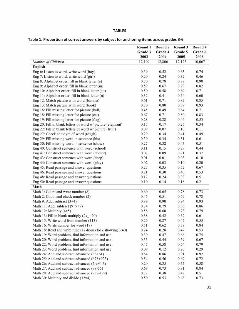
31

TABLES

Table 1: Proportion of correct answers by subject for anchoring items across grades 3-6

Round 1 Grade 3

2003

Round 2 Grade 4

2004

Round 3 Grade 5

2005

Round 4 Grade 6

2006 Number of Children 12,109 12,806 12,123 10,067 English Eng 6: Listen to word, write word (boy) 0.39 0.52 0.65 0.74 Eng 7: Listen to word, write word (girl) 0.20 0.24 0.32 0.46 Eng 8: Alphabet order, fill in blank letter (e) 0.70 0.78 0.88 0.90 Eng 9: Alphabet order, fill in blank letter (m) 0.59 0.67 0.79 0.82 Eng 10: Alphabet order, fill in blank letter (s,t) 0.50 0.58 0.69 0.71 Eng 11: Alphabet order, fill in blank letter (n) 0.32 0.41 0.54 0.60 Eng 12: Match picture with word (banana) 0.61 0.71 0.82 0.85 Eng 13: Match picture with word (book) 0.70 0.80 0.89 0.93 Eng 16: Fill missing letter for picture (ball) 0.45 0.49 0.64 0.71 Eng 18: Fill missing letter for picture (cat) 0.67 0.71 0.80 0.83 Eng 19: Fill missing letter for picture (flag) 0.28 0.28 0.46 0.53 Eng 20: Fill in blank letters of word w/ picture (elephant) 0.17 0.17 0.25 0.34 Eng 22: Fill in blank letters of word w/ picture (fruit) 0.09 0.07 0.10 0.11 Eng 27: Check antonym of word (rough) 0.29 0.34 0.41 0.49 Eng 29: Fill missing word in sentence (his) 0.30 0.34 0.51 0.61 Eng 30: Fill missing word in sentence (show) 0.27 0.32 0.43 0.51 Eng 40: Construct sentence with word (school) 0.11 0.15 0.29 0.44 Eng 41: Construct sentence with word (doctor) 0.07 0.09 0.21 0.37 Eng 43: Construct sentence with word (deep) 0.01 0.01 0.03 0.10 Eng 44: Construct sentence with word (play) 0.02 0.03 0.10 0.20 Eng 45: Read passage and answer questions 0.27 0.35 0.52 0.67 Eng 46: Read passage and answer questions 0.21 0.30 0.40 0.53 Eng 48: Read passage and answer questions 0.17 0.24 0.39 0.51 Eng 50: Read passage and answer questions 0.10 0.14 0.18 0.21 Math Math 1: Count and write number (8) 0.60 0.65 0.78 0.73 Math 2: Count and check number (2) 0.46 0.51 0.69 0.78 Math 9: Add, subtract (3+4) 0.89 0.90 0.94 0.93 Math 11: Add, subtract (9+9+9) 0.74 0.79 0.86 0.86 Math 12: Multiply (4x5) 0.58 0.60 0.73 0.79 Math 13: Fill in blank multiply (2x_=20) 0.38 0.42 0.52 0.61 Math 15: Write word from number (113) 0.26 0.27 0.47 0.55 Math 16: Write number for word (18) 0.51 0.62 0.79 0.84 Math 18: Read and write time (12-hour clock showing 3:40) 0.24 0.28 0.47 0.53 Math 19: Word problem, find information and use 0.39 0.47 0.66 0.75 Math 20: Word problem, find information and use 0.35 0.44 0.59 0.67 Math 22: Word problem, find information and use 0.47 0.58 0.74 0.79 Math 23: Word problem, find information and use 0.09 0.12 0.20 0.29 Math 24: Add and subtract advanced (36+61) 0.84 0.86 0.91 0.92 Math 25: Add and subtract advanced (678+923) 0.54 0.56 0.69 0.72 Math 26: Add and subtract advanced (5.9+4.3) 0.20 0.35 0.55 0.58 Math 27: Add and subtract advanced (98-55) 0.69 0.73 0.81 0.84 Math 28: Add and subtract advanced (238-129) 0.32 0.38 0.48 0.51 Math 30: Multiply and divide (32x4) 0.50 0.53 0.68 0.73

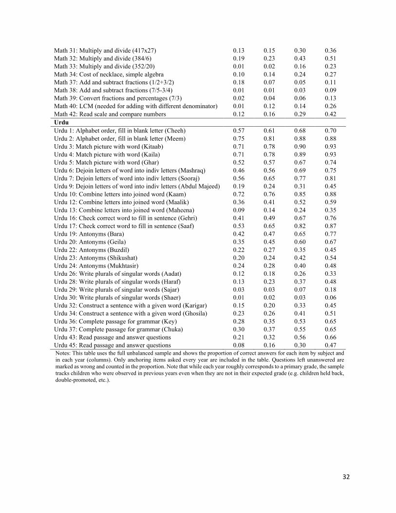
32

Math 31: Multiply and divide (417x27) 0.13 0.15 0.30 0.36 Math 32: Multiply and divide (384/6) 0.19 0.23 0.43 0.51 Math 33: Multiply and divide (352/20) 0.01 0.02 0.16 0.23 Math 34: Cost of necklace, simple algebra 0.10 0.14 0.24 0.27 Math 37: Add and subtract fractions (1/2+3/2) 0.18 0.07 0.05 0.11 Math 38: Add and subtract fractions (7/5-3/4) 0.01 0.01 0.03 0.09 Math 39: Convert fractions and percentages (7/3) 0.02 0.04 0.06 0.13 Math 40: LCM (needed for adding with different denominator) 0.01 0.12 0.14 0.26 Math 42: Read scale and compare numbers 0.12 0.16 0.29 0.42 Urdu Urdu 1: Alphabet order, fill in blank letter (Cheeh) 0.57 0.61 0.68 0.70 Urdu 2: Alphabet order, fill in blank letter (Meem) 0.75 0.81 0.88 0.88 Urdu 3: Match picture with word (Kitaab) 0.71 0.78 0.90 0.93 Urdu 4: Match picture with word (Kaila) 0.71 0.78 0.89 0.93 Urdu 5: Match picture with word (Ghar) 0.52 0.57 0.67 0.74 Urdu 6: Dejoin letters of word into indiv letters (Mashraq) 0.46 0.56 0.69 0.75 Urdu 7: Dejoin letters of word into indiv letters (Sooraj) 0.56 0.65 0.77 0.81 Urdu 9: Dejoin letters of word into indiv letters (Abdul Majeed) 0.19 0.24 0.31 0.45 Urdu 10: Combine letters into joined word (Kaam) 0.72 0.76 0.85 0.88 Urdu 12: Combine letters into joined word (Maalik) 0.36 0.41 0.52 0.59 Urdu 13: Combine letters into joined word (Maheena) 0.09 0.14 0.24 0.35 Urdu 16: Check correct word to fill in sentence (Gehri) 0.41 0.49 0.67 0.76 Urdu 17: Check correct word to fill in sentence (Saaf) 0.53 0.65 0.82 0.87 Urdu 19: Antonyms (Bara) 0.42 0.47 0.65 0.77 Urdu 20: Antonyms (Geila) 0.35 0.45 0.60 0.67 Urdu 22: Antonyms (Buzdil) 0.22 0.27 0.35 0.45 Urdu 23: Antonyms (Shikushat) 0.20 0.24 0.42 0.54 Urdu 24: Antonyms (Mukhtasir) 0.24 0.28 0.40 0.48 Urdu 26: Write plurals of singular words (Aadat) 0.12 0.18 0.26 0.33 Urdu 28: Write plurals of singular words (Haraf) 0.13 0.23 0.37 0.48 Urdu 29: Write plurals of singular words (Sajar) 0.03 0.03 0.07 0.18 Urdu 30: Write plurals of singular words (Shaer) 0.01 0.02 0.03 0.06 Urdu 32: Construct a sentence with a given word (Karigar) 0.15 0.20 0.33 0.45 Urdu 34: Construct a sentence with a given word (Ghosila) 0.23 0.26 0.41 0.51 Urdu 36: Complete passage for grammar (Key) 0.28 0.35 0.53 0.65 Urdu 37: Complete passage for grammar (Chuka) 0.30 0.37 0.55 0.65 Urdu 43: Read passage and answer questions 0.21 0.32 0.56 0.66 Urdu 45: Read passage and answer questions 0.08 0.16 0.30 0.47 Notes: This table uses the full unbalanced sample and shows the proportion of correct answers for each item by subject and in each year (columns). Only anchoring items asked every year are included in the table. Questions left unanswered are marked as wrong and counted in the proportion. Note that while each year roughly corresponds to a primary grade, the sample tracks children who were observed in previous years even when they are not in their expected grade (e.g. children held back, double-promoted, etc.).

33

Table 2: Sample of children by number of years observed, child and household characteristics and mean learning

N Years Observed

N Child-Year Obs.

% Obs.

N Unique Children

Female Proportion

Age (2003)

Avg Days Absent (last

30 days)

% Fathers w/ Primary Edu.

or Less

% Mothers w/ Primary Edu.

or Less

HH Assets PCA

Avg. Annual

Learning

4 24,152 51.27 6,038 0.48 9.58 1.82 44.24 76.13 0.11 0.39 3 14,280 30.32 4,760 0.44 9.69 1.97 51.25 79.07 -0.01 0.40 2 6,088 12.92 3,044 0.38 9.90 2.10 48.50 78.32 -0.09 0.37 1 2,585 5.49 2,585 0.38 9.83 2.42 50.75 78.25 -0.48 -

Notes: This table uses the full unbalanced sample. The “number of years observed” categories are exclusive. Thus, children observed for 1 year are not counted again in other categories. Age in 2003 is estimated for those not observed in that year. Average annual learning is defined as the mean of learning between every year a child is observed. If there are 2- or 3-year gaps, then learning is divided by the number of years in the gap. Father and mother education groups (used to construct % of fathers and mothers with primary education or less) and household assets are not available for every child as these data was only collected for a subsample of children that have test scores. The household assets PCA is the average of all years observed, ignoring missing data. The household assets PCA index is very highly correlated (corr=.96) with an index constructed using IRT on the same household assets (see Appendix Figure 5 for details on how these two measures compare). Fathers’ education, mothers’ education, and household asset information is from the school survey and was cleaned to make it stable across years (see Appendix Table 8 for details on how these variables were cleaned).

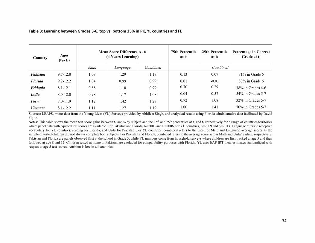
34

Table 3: Learning between Grades 3-6, top vs. bottom 25% in PK, YL countries and FL

Country Ages (t0 - t1)

Mean Score Difference t1 – t0 (4 Years Learning)

75th Percentile at t0

25th Percentile at t1

Percentage in Correct Grade at t1

Math Language Combined Combined

Pakistan 9.7-12.8 1.08 1.29 1.19 0.13 0.07 81% in Grade 6

Florida 9.2-12.2 1.04 0.99 0.99 0.01 -0.01 83% in Grade 6

Ethiopia 8.1-12.1 0.88 1.10 0.99 0.70 0.29 38% in Grades 4-6

India 8.0-12.0 0.98 1.17 1.08 0.04 0.57 54% in Grades 5-7

Peru 8.0-11.9 1.12 1.42 1.27 0.72 1.08 32% in Grades 5-7

Vietnam 8.1-12.2 1.11 1.27 1.19 1.00 1.41 70% in Grades 5-7 Sources: LEAPS, micro-data from the Young Lives (YL) Surveys provided by Abhijeet Singh, and analytical results using Florida administrative data facilitated by David Figlio. Notes: This table shows the mean test score gains between t1 and t0 by subject and the 75th and 25th percentiles at t0 and t1 respectively for a range of countries/territories where panel data with equated test scores are available. For Pakistan and Florida, t0=2003 and t1=2006, for YL countries, t0=2009 and t1=2013. Language refers to receptive vocabulary for YL countries, reading for Florida, and Urdu for Pakistan. For YL countries, combined refers to the mean of Math and Language average scores as the sample of tested children did not always complete both subjects. For Pakistan and Florida, combined refers to the average score across Math and Urdu/reading, respectively. Pakistan and Florida are panels observed first at the school in Grade 3, while YL numbers come from household surveys where children are first tracked at age 5 and then followed at age 8 and 12. Children tested at home in Pakistan are excluded for comparability purposes with Florida. YL uses EAP IRT theta estimates standardized with respect to age 5 test scores. Attrition is low in all countries.

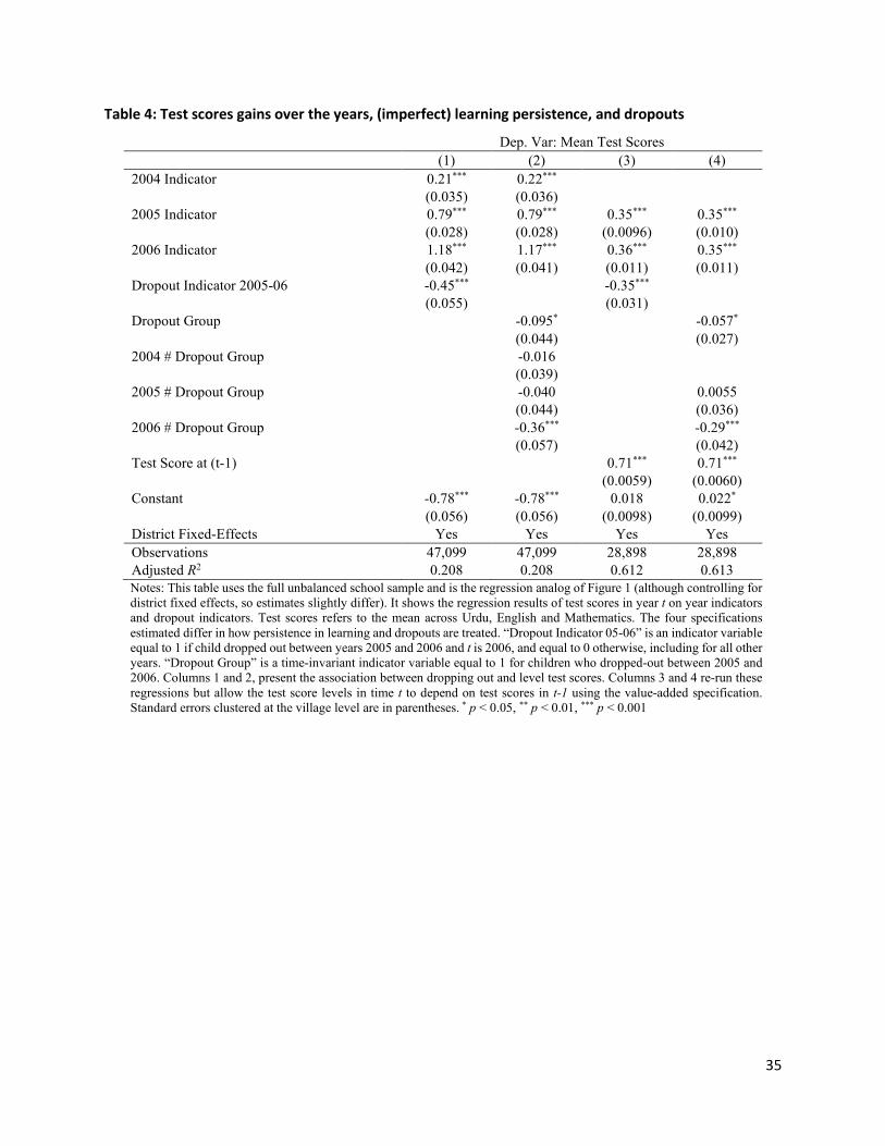
35

Table 4: Test scores gains over the years, (imperfect) learning persistence, and dropouts

Dep. Var: Mean Test Scores (1) (2) (3) (4) 2004 Indicator 0.21*** 0.22*** (0.035) (0.036) 2005 Indicator 0.79*** 0.79*** 0.35*** 0.35*** (0.028) (0.028) (0.0096) (0.010) 2006 Indicator 1.18*** 1.17*** 0.36*** 0.35*** (0.042) (0.041) (0.011) (0.011) Dropout Indicator 2005-06 -0.45*** -0.35*** (0.055) (0.031) Dropout Group -0.095* -0.057* (0.044) (0.027) 2004 # Dropout Group -0.016 (0.039) 2005 # Dropout Group -0.040 0.0055 (0.044) (0.036) 2006 # Dropout Group -0.36*** -0.29*** (0.057) (0.042) Test Score at (t-1) 0.71*** 0.71*** (0.0059) (0.0060) Constant -0.78*** -0.78*** 0.018 0.022* (0.056) (0.056) (0.0098) (0.0099) District Fixed-Effects Yes Yes Yes Yes Observations 47,099 47,099 28,898 28,898 Adjusted R2 0.208 0.208 0.612 0.613 Notes: This table uses the full unbalanced school sample and is the regression analog of Figure 1 (although controlling for district fixed effects, so estimates slightly differ). It shows the regression results of test scores in year t on year indicators and dropout indicators. Test scores refers to the mean across Urdu, English and Mathematics. The four specifications estimated differ in how persistence in learning and dropouts are treated. “Dropout Indicator 05-06” is an indicator variable equal to 1 if child dropped out between years 2005 and 2006 and t is 2006, and equal to 0 otherwise, including for all other years. “Dropout Group” is a time-invariant indicator variable equal to 1 for children who dropped-out between 2005 and 2006. Columns 1 and 2, present the association between dropping out and level test scores. Columns 3 and 4 re-run these regressions but allow the test score levels in time t to depend on test scores in t-1 using the value-added specification. Standard errors clustered at the village level are in parentheses. * p < 0.05, ** p < 0.01, *** p < 0.001

36

Table 5: Test scores over time and learning by quintile

Quintiles by Test Score 2003 Stat

Test Score 2003

Test Score 2004

Test Score 2005

Test Score 2006

Learning (2006-04)

Learning (2006-03)

Quintile 1 Mean -2.01 -1.34 -0.64 -0.26 1.10 1.75 N 1,471 1,314 1,249 1,471 1,314 1,471

Quintile 2 Mean -0.86 -0.55 0.00 0.35 0.92 1.22 N 1,471 1,347 1,275 1,471 1,347 1,471

Quintile 3 Mean -0.38 -0.14 0.37 0.67 0.83 1.05 N 1,471 1,353 1,312 1,471 1,353 1,471

Quintile 4 Mean 0.04 0.19 0.67 0.95 0.77 0.91 N 1,471 1,383 1,332 1,471 1,383 1,471

Quintile 5 Mean 0.62 0.58 1.09 1.33 0.77 0.71 N 1,471 1,358 1,336 1,471 1,358 1,471

All Mean -0.52 -0.24 0.31 0.61 0.88 1.13 N 7,355 6,755 6,504 7,355 6,755 7,355

Notes: This table uses the full unbalanced sample but is restricted to children observed in 2003, since new children in years 2004-06 cannot be classified in quintiles by 2003 test scores. Test scores refers to the mean across Urdu, English and Mathematics. Quintiles by test scores in 2003 are estimated only for those observed in 2006 as their test score in 2006 is needed to estimate their learning. For each quintile, the gains between 2004-06 and 2003-06 are shown. The table shows that measurement error alone does not explain why children who are initially low performers report higher test score gains in our data.

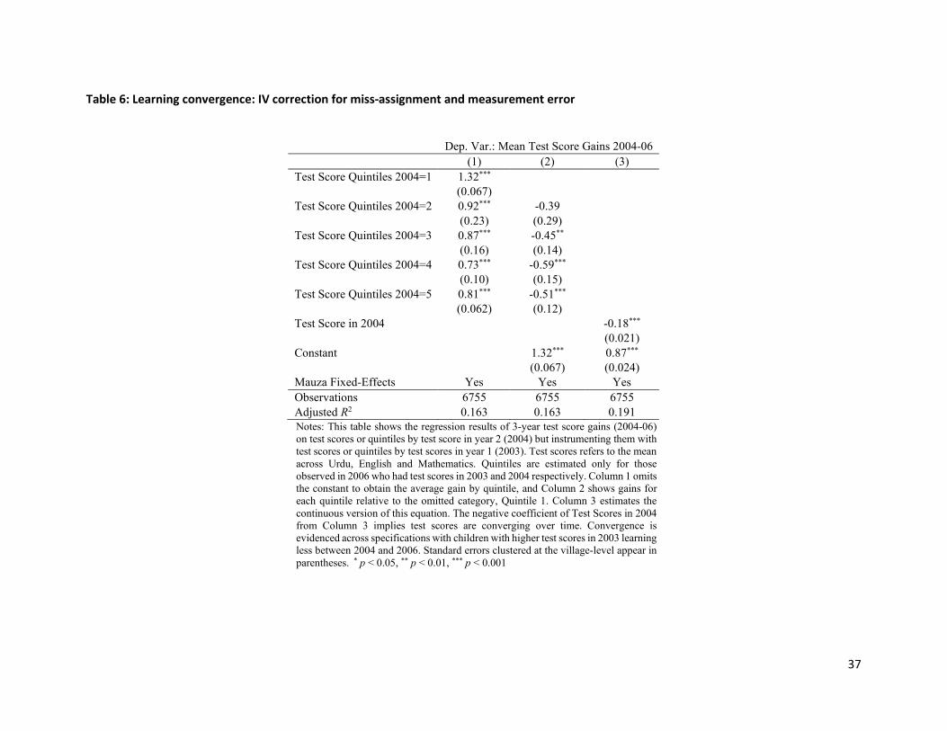
37

Table 6: Learning convergence: IV correction for miss-assignment and measurement error

Dep. Var.: Mean Test Score Gains 2004-06 (1) (2) (3) Test Score Quintiles 2004=1 1.32*** (0.067) Test Score Quintiles 2004=2 0.92*** -0.39 (0.23) (0.29) Test Score Quintiles 2004=3 0.87*** -0.45** (0.16) (0.14) Test Score Quintiles 2004=4 0.73*** -0.59*** (0.10) (0.15) Test Score Quintiles 2004=5 0.81*** -0.51*** (0.062) (0.12) Test Score in 2004 -0.18*** (0.021) Constant 1.32*** 0.87*** (0.067) (0.024) Mauza Fixed-Effects Yes Yes Yes Observations 6755 6755 6755 Adjusted R2 0.163 0.163 0.191 Notes: This table shows the regression results of 3-year test score gains (2004-06) on test scores or quintiles by test score in year 2 (2004) but instrumenting them with test scores or quintiles by test scores in year 1 (2003). Test scores refers to the mean across Urdu, English and Mathematics. Quintiles are estimated only for those observed in 2006 who had test scores in 2003 and 2004 respectively. Column 1 omits the constant to obtain the average gain by quintile, and Column 2 shows gains for each quintile relative to the omitted category, Quintile 1. Column 3 estimates the continuous version of this equation. The negative coefficient of Test Scores in 2004 from Column 3 implies test scores are converging over time. Convergence is evidenced across specifications with children with higher test scores in 2003 learning less between 2004 and 2006. Standard errors clustered at the village-level appear in parentheses. * p < 0.05, ** p < 0.01, *** p < 0.001

38

Table 7: Test scores on lagged test scores, child and household characteristics and fixed effects

(1) (2) (3) (4) Test score t Test score t Test score t Test score t Test Score t-1 0.74*** 0.73*** 0.71*** 0.66*** (0.0058) (0.0060) (0.0064) (0.0076) Father Educ: <Primary -0.0043 -0.0030 -0.0058 (0.013) (0.012) (0.012) Father Educ: >Primary to Higher Secondary 0.070*** 0.074*** 0.064*** (0.0097) (0.0097) (0.0094) Father Educ: Higher Secondary or Higher 0.13*** 0.13*** 0.11*** (0.016) (0.016) (0.016) Mother Educ: <Primary 0.0053 0.0047 -0.0044 (0.011) (0.011) (0.010) Mother Educ: >Primary to Higher Secondary 0.044*** 0.042*** 0.018 (0.0098) (0.0100) (0.0098) Mother Educ: Higher Secondary or Higher 0.085** 0.080** 0.020 (0.027) (0.027) (0.028) Average PCA Asset Index across Years 0.015*** 0.016*** 0.0046 (0.0026) (0.0026) (0.0025) Age in 2003 -0.0093*** -0.0099*** -0.012*** (0.0027) (0.0027) (0.0028) Dropout Group Indicator -0.13*** -0.13*** -0.075*** (0.015) (0.015) (0.017) Female Indicator 0.034*** 0.040*** 0.050*** (0.0075) (0.0075) (0.012) Constant 0.26*** 0.29*** 0.031 -0.63* (0.0070) (0.029) (0.080) (0.27) Mauza Fixed-Effects No No Yes No School Fixed-Effects No No No Yes District Fixed-Effects Yes Yes No No Observations 23,992 23,992 23,992 23,990 Adjusted R-squared 0.59 0.59 0.60 0.64 Within Adjusted R-squared 0.56 0.57 0.54 0.43 Notes: This table uses the full unbalanced panel to regress test scores in year t on lagged test scores at t-1 along with parental education groups, average wealth across rounds, baseline age, sex and whether the child dropped-out in 2005-06. Test scores refers to the mean across Urdu, English and Mathematics. Specifications across columns include a full set of village or school fixed effects to capture potential differences by geography and schools. The Within Adjusted R-square measures the explanatory power net of mauza, school and district fixed-effects respectively. Household and child characteristics explain very little of the variation in test score gains after accounting for fixed effects. Standard errors clustered at the village-level are in parentheses. The base category for the father and mother education groups is no education. The average wealth measure ignores missing data in any given year. * p < 0.05, ** p < 0.01, *** p < 0.001

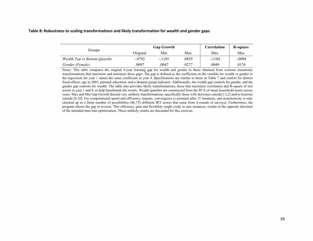
39

Table 8: Robustness to scaling transformations and likely transformation for wealth and gender gaps

Groups Gap Growth Correlation R-square

Original Min Max Max Max Wealth Top vs Bottom Quartile -.0792 -.1185 .0829 -.1184 -.0094 Gender (Female) .0097 .0047 .0277 .0049 .0176 Notes: This table compares the original 4-year learning gap for wealth and gender to those obtained from extreme monotonic transformations that maximize and minimize these gaps. The gap is defined as the coefficient on the variable for wealth or gender in the regression for year 1 minus the same coefficient in year 4. Specifications are similar to those in Table 7 and control for district fixed effects, age in 2003, parental education, and a dropout group indicator. Additionally, the wealth gap controls for gender, and the gender gap controls for wealth. The table also provides likely transformations, those that maximize correlation and R-square of test scores in year 1 and 4, to help benchmark the results. Wealth quartiles are constructed from the PCA of mean household assets across years. Max and Min Gap Growth discard very unlikely transformations, specifically those with skewness outside [-2,2] and/or kurtosis outside [0,10]. For computational speed and efficiency reasons, convergence is assumed after 15 iterations, and monotonicity is only checked up to a finite number of possibilities (46,735 different IRT scores that came from 4 rounds of surveys). Furthermore, the program allows the gap to reverse. This efficiency gain and flexibility might yield, in rare instances, results in the opposite direction of the intended max/min optimization. These unlikely results are discarded for this exercise.

40

FIGURES

Figure 1: Learning trajectories for 2005 dropouts, non-dropouts and difference – combined test scores

Panel A Panel B

Notes: Panel A shows test scores in every round for two groups of students in the full unbalanced school panel. The red solid line shows students who were enrolled in every year, while the dotted blue line shows test scores in every round for students who eventually dropped-out in the transition from primary to middle school. The last score for the dropout group reflects their scores when they were tested at home and have been out of school for one year. 95% confidence intervals displayed for each year-group combination. The percentage of dropouts in 2006 is 11.89%. Panel B shows the difference in test scores between both groups for each year and its corresponding 95% confidence interval. Test scores refers to the mean across Urdu, English and Mathematics.

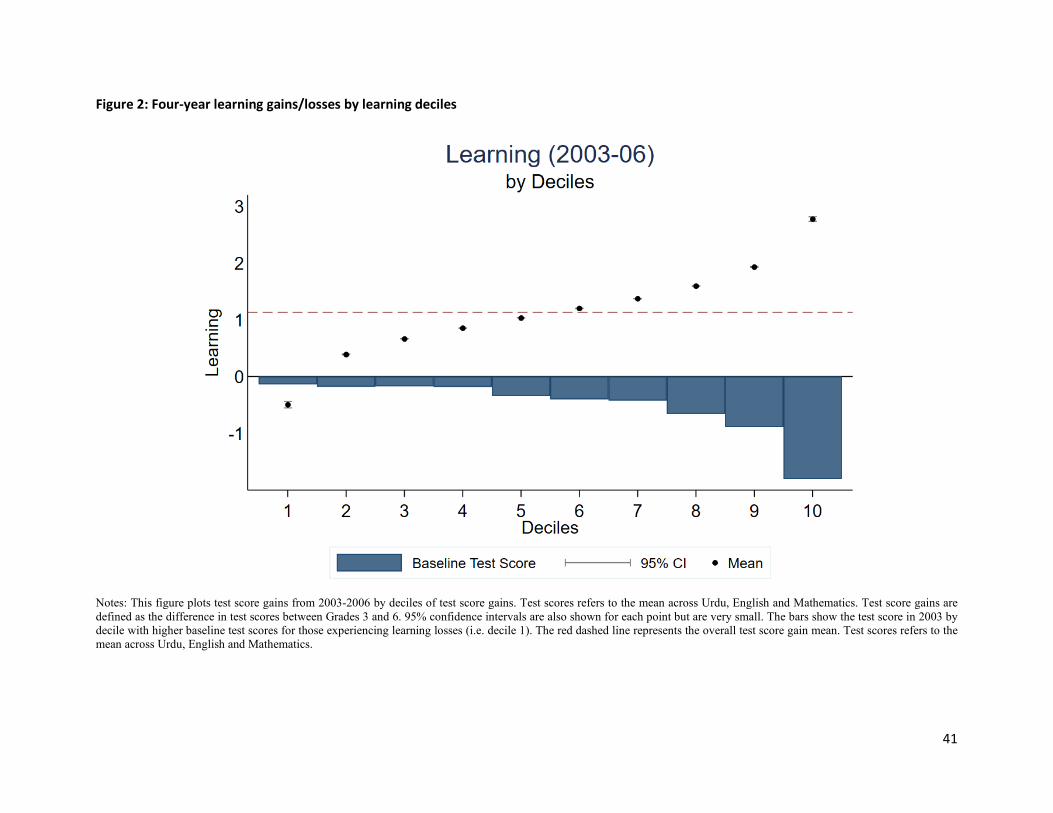
41

Figure 2: Four-year learning gains/losses by learning deciles

Notes: This figure plots test score gains from 2003-2006 by deciles of test score gains. Test scores refers to the mean across Urdu, English and Mathematics. Test score gains are defined as the difference in test scores between Grades 3 and 6. 95% confidence intervals are also shown for each point but are very small. The bars show the test score in 2003 by decile with higher baseline test scores for those experiencing learning losses (i.e. decile 1). The red dashed line represents the overall test score gain mean. Test scores refers to the mean across Urdu, English and Mathematics.

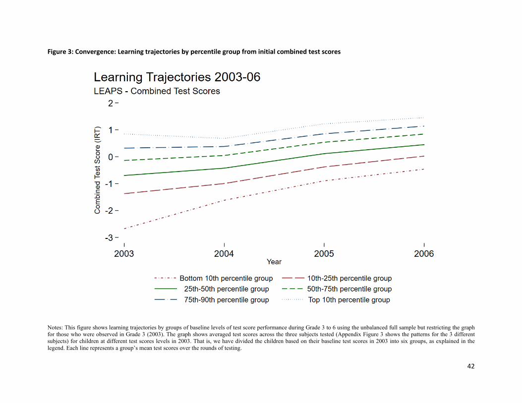
42

Figure 3: Convergence: Learning trajectories by percentile group from initial combined test scores

Notes: This figure shows learning trajectories by groups of baseline levels of test score performance during Grade 3 to 6 using the unbalanced full sample but restricting the graph for those who were observed in Grade 3 (2003). The graph shows averaged test scores across the three subjects tested (Appendix Figure 3 shows the patterns for the 3 different subjects) for children at different test scores levels in 2003. That is, we have divided the children based on their baseline test scores in 2003 into six groups, as explained in the legend. Each line represents a group’s mean test scores over the rounds of testing.

43

Figure 4: Proportion of fragile and robust learners by subject

Notes: This figure examines the proportion of students from the balanced panel (i.e. those observed every year, N=6,038) that, for each anchoring question asked every year, can be classified, based on the pattern of their correct/incorrect answer, as: (i) robust learners: those whose trajectories show (weakly) monotonic progression starting from a point where they could not answer the question; and (ii) fragile learners: those whose trajectories show regression at some point. The proportion of fragile to robust learners is shown at the top of each bar. An asterisk before the question indicates that the item was a multiple-choice questions (MCQ). The missing proportion corresponds to always or never learners, those who always or never answered correctly a given item.

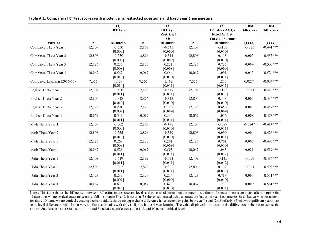
44

Table A.1: Comparing IRT test scores with model using restricted questions and fixed year 1 parameters

(1)

(2) (3) t-test t-test IRT 4yrs

IRT 4yrs

Restricted Qs

IRT 4yrs All Qs Fixed Yr 1 &

Varying Params

Difference Difference

Variable N Mean/SE N Mean/SE N Mean/SE (1)-(2) (1)-(3) Combined Theta Year 1 12,109 -0.550 12,109 -0.535 12,109 -0.108 -0.015 -0.441***

[0.009]

[0.009] [0.010]

Combined Theta Year 2 12,806 -0.339 12,806 -0.341 12,806 0.115 0.003 -0.453*** [0.009]

[0.009] [0.010]

Combined Theta Year 3 12,123 0.235 12,123 0.231 12,123 0.735 0.004 -0.500*** [0.008]

[0.008] [0.009]

Combined Theta Year 4 10,067 0.567 10,067 0.554 10,067 1.091 0.013 -0.524*** [0.010]

[0.010] [0.011]

Combined Learning (2006-03) 7,355 1.129 7,355 1.102 7,355 1.213 0.027* -0.084*** [0.010]

[0.011] [0.011]

English Theta Year 1 12,109 -0.528 12,109 -0.517 12,109 -0.102 -0.011 -0.426*** [0.011]

[0.011] [0.012]

English Theta Year 2 12,806 -0.318 12,806 -0.323 12,806 0.118 0.005 -0.436*** [0.010]

[0.010] [0.010]

English Theta Year 3 12,123 0.201 12,123 0.198 12,123 0.658 0.003 -0.457*** [0.009]

[0.009] [0.009]

English Theta Year 4 10,067 0.542 10,067 0.534 10,067 1.016 0.008 -0.473*** [0.011]

[0.011] [0.011]

Math Theta Year 1 12,109 -0.502 12,109 -0.478 12,109 -0.087 -0.024* -0.414*** [0.009]

[0.010] [0.011]

Math Theta Year 2 12,806 -0.335 12,806 -0.339 12,806 0.090 0.004 -0.426*** [0.010]

[0.010] [0.011]

Math Theta Year 3 12,123 0.268 12,123 0.261 12,123 0.761 0.007 -0.493*** [0.009]

[0.009] [0.010]

Math Theta Year 4 10,067 0.526 10,067 0.505 10,067 1.045 0.021 -0.519*** [0.011]

[0.011] [0.012]

Urdu Theta Year 1 12,109 -0.619 12,109 -0.611 12,109 -0.135 -0.009 -0.484*** [0.011]

[0.011] [0.012]

Urdu Theta Year 2 12,806 -0.362 12,806 -0.362 12,806 0.137 -0.001 -0.499*** [0.011]

[0.011] [0.012]

Urdu Theta Year 3 12,123 0.237 12,123 0.234 12,123 0.788 0.003 -0.551*** [0.009]

[0.009] [0.010]

Urdu Theta Year 4 10,067 0.632 10,067 0.623 10,067 1.213 0.009 -0.581*** [0.010]

[0.010] [0.011]

Notes: This table shows the differences between IRT-estimated tests scores levels and gains used throughout the paper (i.e. column 1) versus: those recomputed after dropping the 19 questions where vertical equating seems to fail in column (2); and, in column (3), those recomputed using all questions but using year 1 parameters for all but varying parameters for those 19 items where vertical equating seems to fail. It shows no appreciable difference in test scores or gains between (1) and (2). Similarly, (3) shows significant yearly test score level differences with (1) but very similar yearly gains with only a slightly larger 4-year learning. The value displayed for t-tests are the differences in the means across the groups. Standard errors are robust. ***, **, and * indicate significance at the 1, 5, and 10 percent critical level.

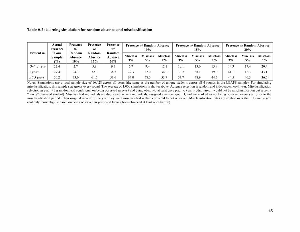
45

Table A.2: Learning simulation for random absence and misclassification

Present in

Actual Presence

in our Sample

(%)

Presence w/

Random Absence

10%

Presence w/

Random Absence

15%

Presence w/

Random Absence

20%

Presence w/ Random Absence 10%

Presence w/ Random Absence 15%

Presence w/ Random Absence 20%

Misclass 3%

Misclass 5%

Misclass 7%

Misclass 3%

Misclass 5%

Misclass 7%

Misclass 3%

Misclass 5%

Misclass 7%

Only 1 year 22.4 2.7 5.8 9.7 6.7 9.4 12.1 10.1 13.0 15.9 14.3 17.4 20.4 2 years 27.4 24.3 32.6 38.7 29.3 32.0 34.2 36.2 38.1 39.6 41.1 42.3 43.1 All 3 years 50.2 73.0 61.6 51.6 64.0 58.6 53.7 53.7 48.9 44.5 44.5 40.3 36.5

Notes: Simulations use a total sample size of 16,428 across all years (the same as the number of unique students across all 4 rounds in the LEAPS sample). For simulating misclassification, this sample size grows every round. The average of 1,000 simulations is shown above. Absence selection is random and independent each year. Misclassification selection in year t+1 is random and conditional on being observed in year t and being observed at least once prior to year t (otherwise, it would not be misclassification but rather a “newly” observed student). Misclassified individuals are duplicated as new individuals, assigned a new unique ID, and are marked as not being observed every year prior to the misclassification period. Their original record for the year they were misclassified is then corrected to not observed. Misclassification rates are applied over the full sample size (not only those eligible based on being observed in year t and having been observed at least once before).

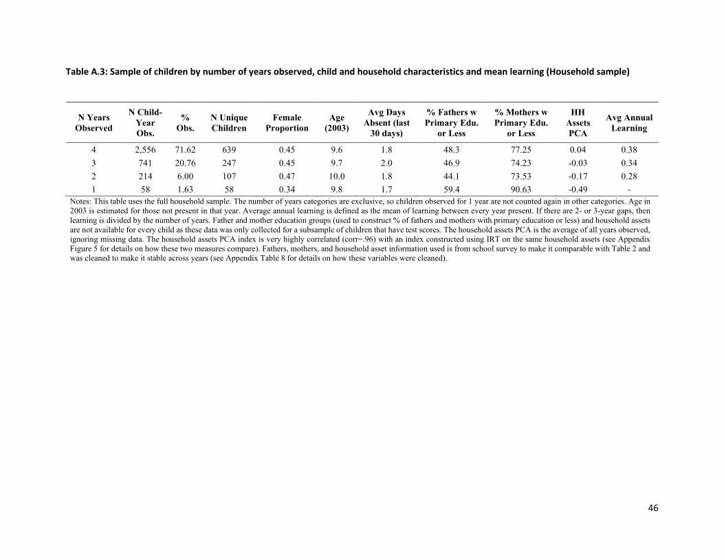
46

Table A.3: Sample of children by number of years observed, child and household characteristics and mean learning (Household sample)

N Years Observed

N Child-Year Obs.

% Obs.

N Unique Children

Female Proportion

Age (2003)

Avg Days Absent (last

30 days)

% Fathers w Primary Edu.

or Less

% Mothers w Primary Edu.

or Less

HH Assets PCA

Avg Annual Learning

4 2,556 71.62 639 0.45 9.6 1.8 48.3 77.25 0.04 0.38 3 741 20.76 247 0.45 9.7 2.0 46.9 74.23 -0.03 0.34 2 214 6.00 107 0.47 10.0 1.8 44.1 73.53 -0.17 0.28 1 58 1.63 58 0.34 9.8 1.7 59.4 90.63 -0.49 -

Notes: This table uses the full household sample. The number of years categories are exclusive, so children observed for 1 year are not counted again in other categories. Age in 2003 is estimated for those not present in that year. Average annual learning is defined as the mean of learning between every year present. If there are 2- or 3-year gaps, then learning is divided by the number of years. Father and mother education groups (used to construct % of fathers and mothers with primary education or less) and household assets are not available for every child as these data was only collected for a subsample of children that have test scores. The household assets PCA is the average of all years observed, ignoring missing data. The household assets PCA index is very highly correlated (corr=.96) with an index constructed using IRT on the same household assets (see Appendix Figure 5 for details on how these two measures compare). Fathers, mothers, and household asset information used is from school survey to make it comparable with Table 2 and was cleaned to make it stable across years (see Appendix Table 8 for details on how these variables were cleaned).

47

Table A.4: Learning for unbalanced, balanced, and household panels

Variable

(1) (2) (3) t-test t-test t-test

Unbalanced Panel Balanced Panel Household Panel Difference Difference Difference

N Mean/SE N Mean/SE N Mean/SE (1)-(2) (1)-(3) (2)-(3) Learning 2003-06 7,355 1.129 6,038 1.155 1,406 1.101 -0.026* 0.028 0.054*

[0.010] [0.011] [0.025] Learning 2004-06 8,470 0.889 6,038 0.884 1,417 0.833 0.006 0.056** 0.051**

[0.008] [0.009] [0.022] Learning 2005-06 8,796 0.355 6,038 0.344 1,412 0.305 0.011 0.050** 0.040*

[0.007] [0.008] [0.019] Learning 2003-05 8,829 0.799 6,038 0.811 1,404 0.813 -0.012 -0.014 -0.003

[0.008] [0.009] [0.019] Learning 2004-05 10,212 0.537 6,038 0.539 1,427 0.542 -0.002 -0.004 -0.003

[0.006] [0.007] [0.015] Learning 2003-05 9,890 0.258 6,038 0.272 1,450 0.284 -0.014 -0.026 -0.012 [0.008] [0.010] [0.020] Notes: This tables compares learning for 3 different samples: (i) a balanced sample of 6,038 children who were present in every year; (ii) the full unbalanced samples of children present in different years; and (iii) the household sample where the balanced proportion is higher. It shows that test score gains are very similar across all three samples, with statistically significant differences between the unbalanced/balanced panels when comparing against the household panel only when learning includes year 4. This is likely caused by the inclusion of testing dropouts at home and the fact that the balanced panel itself is a (slightly) selected group of children. The value displayed for t-tests are the differences in the means across the groups. Standard errors are robust and shown in brackets. ***, **, and * indicate significance at the 1, 5, and 10 percent critical level.

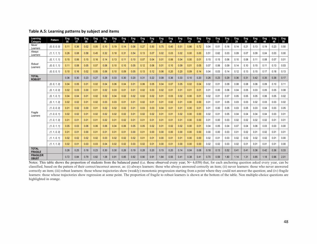
48

Table A.5: Learning patterns by subject and items Learning Category Pattern Eng

06 Eng 07

Eng 08

Eng 09

Eng 10

Eng 11

Eng 16

Eng 18

Eng 19

Eng 20

Eng 22

Eng 40

Eng 41

Eng 43

Eng 44

Eng 12

Eng 13

Eng 27

Eng 29

Eng 30

Eng 45

Eng 46

Eng 48

Eng 50

Never Learners (0, 0, 0, 0) 0.11 0.36 0.02 0.05 0.10 0.19 0.14 0.06 0.27 0.50 0.75 0.40 0.51 0.86 0.72 0.04 0.01 0.16 0.14 0.21 0.13 0.19 0.23 0.50

Always Learners (1, 1, 1, 1) 0.26 0.08 0.58 0.45 0.32 0.18 0.31 0.54 0.13 0.07 0.02 0.03 0.02 0.00 0.00 0.51 0.62 0.03 0.09 0.07 0.09 0.04 0.03 0.00

Robust Learners

(0, 1, 1, 1) 0.15 0.06 0.15 0.16 0.14 0.13 0.11 0.10 0.07 0.04 0.01 0.06 0.04 0.00 0.01 0.15 0.15 0.06 0.10 0.08 0.11 0.08 0.07 0.01

(0, 0, 1, 1) 0.11 0.08 0.05 0.07 0.08 0.10 0.10 0.05 0.12 0.06 0.01 0.10 0.09 0.01 0.05 0.07 0.06 0.09 0.14 0.10 0.15 0.11 0.13 0.03

(0, 0, 0, 1) 0.10 0.16 0.02 0.05 0.06 0.10 0.09 0.05 0.13 0.12 0.06 0.20 0.20 0.09 0.14 0.04 0.03 0.14 0.12 0.13 0.15 0.17 0.18 0.13 TOTAL ROBUST

0.36 0.30 0.23 0.27 0.28 0.33 0.30 0.20 0.31 0.22 0.08 0.36 0.33 0.10 0.20 0.26 0.23 0.29 0.36 0.31 0.42 0.35 0.38 0.17

Fragile Learners

(0, 0, 1, 0) 0.04 0.05 0.01 0.02 0.04 0.06 0.04 0.01 0.06 0.05 0.04 0.07 0.05 0.02 0.04 0.02 0.01 0.09 0.08 0.08 0.06 0.09 0.10 0.11

(0, 1, 0, 0) 0.02 0.03 0.00 0.01 0.02 0.03 0.01 0.01 0.02 0.03 0.02 0.01 0.01 0.01 0.01 0.01 0.00 0.06 0.04 0.05 0.03 0.05 0.05 0.08

(0, 1, 0, 1) 0.04 0.04 0.01 0.02 0.02 0.04 0.02 0.02 0.02 0.02 0.01 0.03 0.02 0.00 0.01 0.02 0.01 0.07 0.05 0.05 0.05 0.06 0.05 0.02

(0, 1, 1, 0) 0.02 0.02 0.01 0.02 0.03 0.03 0.01 0.01 0.02 0.01 0.01 0.02 0.01 0.00 0.00 0.01 0.01 0.05 0.03 0.03 0.02 0.03 0.03 0.02

(1, 0, 0, 0) 0.01 0.02 0.00 0.01 0.02 0.02 0.02 0.01 0.03 0.03 0.04 0.01 0.01 0.00 0.01 0.01 0.00 0.05 0.03 0.05 0.03 0.04 0.03 0.05

(1, 0, 0, 1) 0.02 0.02 0.01 0.02 0.02 0.02 0.02 0.01 0.02 0.02 0.01 0.01 0.02 0.00 0.00 0.02 0.01 0.05 0.04 0.04 0.04 0.04 0.03 0.01

(1, 0, 1, 0) 0.01 0.01 0.01 0.01 0.02 0.01 0.02 0.01 0.01 0.01 0.01 0.01 0.01 0.00 0.00 0.01 0.00 0.03 0.02 0.02 0.02 0.02 0.01 0.01

(1, 0, 1, 1) 0.05 0.03 0.06 0.06 0.06 0.04 0.06 0.05 0.05 0.02 0.01 0.02 0.02 0.00 0.01 0.04 0.05 0.04 0.07 0.04 0.06 0.03 0.03 0.00

(1, 1, 0, 0) 0.01 0.01 0.00 0.01 0.01 0.01 0.01 0.00 0.01 0.00 0.00 0.00 0.00 0.00 0.00 0.00 0.00 0.03 0.01 0.02 0.01 0.02 0.01 0.01

(1, 1, 0, 1) 0.02 0.02 0.02 0.02 0.03 0.02 0.02 0.02 0.01 0.01 0.00 0.01 0.01 0.00 0.00 0.02 0.01 0.03 0.02 0.02 0.02 0.02 0.01 0.00

(1, 1, 1, 0) 0.02 0.01 0.03 0.03 0.04 0.02 0.02 0.03 0.02 0.01 0.00 0.01 0.00 0.00 0.00 0.02 0.02 0.03 0.02 0.01 0.01 0.01 0.01 0.00 TOTAL FRAGILE

0.26 0.25 0.18 0.23 0.30 0.30 0.26 0.19 0.28 0.20 0.15 0.20 0.14 0.04 0.08 0.18 0.13 0.52 0.41 0.41 0.36 0.42 0.36 0.33

FRAGILE/ROBUST

0.72 0.84 0.79 0.82 1.08 0.91 0.85 0.92 0.90 0.91 1.84 0.55 0.41 0.38 0.41 0.70 0.59 1.80 1.14 1.31 0.85 1.18 0.96 2.01

Notes: This table shows the proportion of students from the balanced panel (i.e. those observed every year; N= 6,038) that, for each anchoring question asked every year, can be classified, based on the pattern of their correct/incorrect answer, as: (i) always learners: those who always answered correctly an item; (ii) never learners: those who never answered correctly an item; (iii) robust learners: those whose trajectories show (weakly) monotonic progression starting from a point where they could not answer the question; and (iv) fragile learners: those whose trajectories show regression at some point. The proportion of fragile to robust learners is shown at the bottom of the table. Non multiple-choice questions are highlighted in orange.

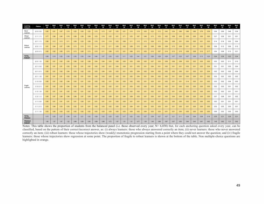
49

Learning Category

Pattern Math 09

Math 11

Math 12

Math 13

Math 15

Math 16

Math 18

Math 19

Math 20

Math 22

Math 23

Math 24

Math 25

Math 26

Math 27

Math 28

Math 30

Math 31

Math 32

Math 33

Math 37

Math 38

Math 39

Math 40

Math 01

Math 02

Math 34

Math 42

Never Learners

(0, 0, 0, 0) 0.00 0.01 0.07 0.16 0.25 0.05 0.25 0.10 0.13 0.07 0.50 0.01 0.10 0.19 0.03 0.23 0.12 0.43 0.34 0.66 0.66 0.86 0.79 0.59 0.04 0.06 0.48 0.34

Always Learners

(1, 1, 1, 1) 0.77 0.56 0.40 0.18 0.09 0.38 0.09 0.23 0.18 0.32 0.01 0.71 0.33 0.07 0.49 0.13 0.33 0.02 0.09 0.00 0.00 0.00 0.00 0.00 0.37 0.26 0.01 0.01

Robust Learners

(0, 1, 1, 1) 0.06 0.12 0.13 0.11 0.09 0.20 0.09 0.16 0.14 0.18 0.03 0.08 0.11 0.15 0.13 0.09 0.12 0.04 0.08 0.01 0.00 0.00 0.01 0.03 0.14 0.18 0.03 0.04

(0, 0, 1, 1) 0.01 0.04 0.07 0.09 0.13 0.10 0.12 0.14 0.12 0.11 0.06 0.02 0.08 0.15 0.05 0.08 0.08 0.09 0.15 0.08 0.01 0.01 0.02 0.05 0.06 0.12 0.06 0.10

(0, 0, 0, 1) 0.00 0.02 0.05 0.10 0.13 0.05 0.13 0.10 0.11 0.06 0.15 0.01 0.06 0.12 0.03 0.10 0.07 0.14 0.13 0.15 0.06 0.08 0.10 0.17 0.04 0.08 0.13 0.21

TOTAL ROBUST

0.08 0.18 0.25 0.30 0.35 0.35 0.34 0.40 0.37 0.35 0.23 0.11 0.25 0.41 0.21 0.26 0.28 0.28 0.37 0.23 0.07 0.09 0.13 0.25 0.24 0.38 0.22 0.34

Fragile Learners

(0, 0, 1, 0) 0.00 0.01 0.02 0.05 0.06 0.02 0.08 0.04 0.04 0.03 0.08 0.00 0.03 0.08 0.02 0.07 0.03 0.09 0.06 0.08 0.03 0.02 0.03 0.05 0.03 0.03 0.11 0.10

(0, 1, 0, 0) 0.00 0.01 0.01 0.03 0.02 0.01 0.02 0.02 0.02 0.01 0.04 0.00 0.01 0.03 0.01 0.04 0.01 0.02 0.01 0.01 0.03 0.01 0.02 0.04 0.01 0.01 0.05 0.04

(0, 1, 0, 1) 0.00 0.01 0.02 0.04 0.03 0.02 0.03 0.03 0.04 0.03 0.03 0.01 0.03 0.04 0.02 0.04 0.02 0.02 0.02 0.00 0.01 0.00 0.01 0.04 0.02 0.03 0.02 0.04

(0, 1, 1, 0) 0.01 0.01 0.01 0.03 0.02 0.01 0.03 0.02 0.03 0.02 0.02 0.01 0.02 0.04 0.01 0.04 0.02 0.02 0.01 0.00 0.00 0.00 0.01 0.02 0.03 0.02 0.02 0.02

(1, 0, 0, 0) 0.00 0.01 0.02 0.04 0.03 0.01 0.03 0.02 0.02 0.01 0.04 0.00 0.02 0.02 0.01 0.03 0.01 0.02 0.01 0.01 0.14 0.00 0.01 0.00 0.03 0.02 0.04 0.03

(1, 0, 0, 1) 0.01 0.02 0.03 0.04 0.02 0.02 0.02 0.03 0.03 0.02 0.01 0.01 0.03 0.02 0.02 0.03 0.02 0.02 0.01 0.00 0.02 0.00 0.00 0.00 0.02 0.03 0.01 0.02

(1, 0, 1, 0) 0.01 0.01 0.01 0.02 0.02 0.01 0.02 0.01 0.02 0.01 0.01 0.01 0.02 0.02 0.01 0.02 0.01 0.02 0.01 0.00 0.01 0.00 0.00 0.00 0.03 0.02 0.01 0.01

(1, 0, 1, 1) 0.05 0.07 0.08 0.06 0.06 0.07 0.05 0.07 0.06 0.06 0.01 0.06 0.08 0.03 0.07 0.05 0.07 0.03 0.04 0.00 0.00 0.00 0.00 0.00 0.07 0.08 0.01 0.02

(1, 1, 0, 0) 0.00 0.01 0.01 0.01 0.01 0.00 0.01 0.01 0.01 0.01 0.00 0.00 0.01 0.01 0.01 0.02 0.01 0.01 0.00 0.00 0.02 0.00 0.00 0.00 0.02 0.01 0.01 0.01

(1, 1, 0, 1) 0.03 0.04 0.03 0.03 0.02 0.01 0.01 0.02 0.03 0.02 0.00 0.03 0.04 0.01 0.04 0.03 0.03 0.01 0.01 0.00 0.01 0.00 0.00 0.00 0.03 0.03 0.00 0.01

(1, 1, 1, 0) 0.03 0.05 0.03 0.02 0.02 0.02 0.02 0.02 0.03 0.03 0.00 0.03 0.05 0.02 0.04 0.03 0.03 0.01 0.01 0.00 0.00 0.00 0.00 0.00 0.06 0.02 0.00 0.00

TOTAL FRAGILE

0.15 0.25 0.27 0.36 0.31 0.21 0.32 0.28 0.32 0.25 0.25 0.17 0.32 0.32 0.27 0.39 0.27 0.27 0.21 0.11 0.26 0.04 0.08 0.16 0.35 0.31 0.29 0.31

FRAGILE/ROBUST

1.83 1.37 1.07 1.22 0.89 0.59 0.93 0.69 0.88 0.72 1.07 1.51 1.31 0.77 1.30 1.49 0.98 0.97 0.57 0.50 3.64 0.43 0.61 0.62 1.49 0.82 1.31 0.92

Notes: This table shows the proportion of students from the balanced panel (i.e. those observed every year; N= 6,038) that, for each anchoring question asked every year, can be classified, based on the pattern of their correct/incorrect answer, as: (i) always learners: those who always answered correctly an item; (ii) never learners: those who never answered correctly an item; (iii) robust learners: those whose trajectories show (weakly) monotonic progression starting from a point where they could not answer the question; and (iv) fragile learners: those whose trajectories show regression at some point. The proportion of fragile to robust learners is shown at the bottom of the table. Non multiple-choice questions are highlighted in orange.

50

Learning Category

Pattern Urdu 01

Urdu 02

Urdu 06

Urdu 07

Urdu 09

Urdu 10

Urdu 12

Urdu 13

Urdu 26

Urdu 28

Urdu 29

Urdu 30

Urdu 32

Urdu 34

Urdu 45

Urdu 03

Urdu 04

Urdu 05

Urdu 16

Urdu 17

Urdu 19

Urdu 20

Urdu 22

Urdu 23

Urdu 24

Urdu 36

Urdu 37

Urdu 43

Never Learners

(0, 0, 0, 0) 0.09 0.01 0.10 0.06 0.36 0.03 0.21 0.50 0.45 0.32 0.75 0.89 0.37 0.32 0.37 0.01 0.01 0.07 0.09 0.03 0.07 0.10 0.25 0.21 0.21 0.14 0.15 0.16

Always Learners

(1, 1, 1, 1) 0.33 0.58 0.34 0.44 0.06 0.59 0.21 0.03 0.03 0.04 0.00 0.00 0.05 0.11 0.03 0.62 0.61 0.30 0.26 0.38 0.22 0.16 0.03 0.03 0.04 0.10 0.14 0.10

Robust Learners

(0, 1, 1, 1) 0.12 0.13 0.15 0.15 0.05 0.12 0.10 0.05 0.04 0.09 0.01 0.00 0.08 0.09 0.07 0.15 0.15 0.12 0.16 0.19 0.15 0.15 0.06 0.07 0.07 0.13 0.14 0.15

(0, 0, 1, 1) 0.06 0.04 0.09 0.08 0.08 0.05 0.08 0.08 0.07 0.12 0.03 0.01 0.10 0.09 0.14 0.05 0.05 0.08 0.13 0.11 0.14 0.12 0.09 0.16 0.10 0.14 0.14 0.18

(0, 0, 0, 1) 0.05 0.01 0.08 0.05 0.15 0.02 0.11 0.16 0.15 0.17 0.14 0.06 0.16 0.14 0.21 0.02 0.02 0.07 0.10 0.05 0.09 0.10 0.14 0.17 0.14 0.13 0.13 0.14

TOTAL ROBUST

0.22 0.18 0.32 0.27 0.28 0.19 0.30 0.29 0.26 0.38 0.18 0.07 0.34 0.32 0.42 0.22 0.22 0.27 0.39 0.35 0.38 0.36 0.29 0.39 0.31 0.40 0.40 0.48

Fragile Learners

(0, 0, 1, 0) 0.03 0.01 0.03 0.02 0.06 0.01 0.04 0.05 0.07 0.07 0.02 0.02 0.05 0.05 0.06 0.01 0.01 0.03 0.04 0.02 0.04 0.06 0.08 0.08 0.09 0.06 0.05 0.06

(0, 1, 0, 0) 0.02 0.01 0.01 0.01 0.03 0.01 0.03 0.02 0.04 0.04 0.01 0.01 0.02 0.01 0.02 0.00 0.01 0.03 0.02 0.01 0.02 0.03 0.06 0.04 0.06 0.02 0.02 0.02

(0, 1, 0, 1) 0.03 0.02 0.03 0.02 0.04 0.02 0.03 0.02 0.03 0.03 0.01 0.00 0.03 0.03 0.03 0.01 0.02 0.04 0.03 0.03 0.04 0.05 0.05 0.04 0.05 0.05 0.04 0.04

(0, 1, 1, 0) 0.02 0.02 0.02 0.02 0.02 0.01 0.02 0.01 0.03 0.02 0.00 0.00 0.02 0.02 0.01 0.01 0.01 0.03 0.02 0.02 0.02 0.03 0.03 0.03 0.03 0.03 0.03 0.02

(1, 0, 0, 0) 0.04 0.01 0.02 0.01 0.02 0.01 0.03 0.01 0.03 0.02 0.02 0.01 0.02 0.02 0.01 0.00 0.00 0.03 0.02 0.01 0.02 0.03 0.05 0.04 0.05 0.02 0.02 0.01

(1, 0, 0, 1) 0.03 0.01 0.02 0.02 0.02 0.02 0.03 0.01 0.01 0.02 0.00 0.00 0.02 0.02 0.01 0.01 0.01 0.03 0.03 0.02 0.04 0.03 0.04 0.04 0.04 0.04 0.03 0.02

(1, 0, 1, 0) 0.02 0.01 0.01 0.01 0.01 0.01 0.01 0.01 0.01 0.01 0.00 0.00 0.01 0.02 0.00 0.01 0.01 0.02 0.01 0.01 0.02 0.02 0.03 0.02 0.03 0.02 0.02 0.01

(1, 0, 1, 1) 0.07 0.07 0.05 0.05 0.03 0.06 0.04 0.01 0.01 0.02 0.00 0.00 0.03 0.05 0.02 0.06 0.06 0.07 0.06 0.08 0.09 0.06 0.03 0.04 0.04 0.06 0.06 0.04

(1, 1, 0, 0) 0.02 0.00 0.01 0.01 0.01 0.01 0.01 0.00 0.01 0.01 0.00 0.00 0.01 0.00 0.00 0.00 0.00 0.02 0.01 0.00 0.01 0.01 0.02 0.01 0.02 0.01 0.01 0.00

(1, 1, 0, 1) 0.04 0.03 0.02 0.02 0.03 0.03 0.02 0.00 0.01 0.01 0.00 0.00 0.01 0.02 0.01 0.02 0.02 0.04 0.02 0.03 0.02 0.03 0.02 0.01 0.02 0.03 0.02 0.01

(1, 1, 1, 0) 0.04 0.05 0.02 0.02 0.01 0.02 0.02 0.00 0.01 0.01 0.00 0.00 0.01 0.02 0.00 0.02 0.01 0.03 0.02 0.02 0.02 0.02 0.01 0.01 0.01 0.02 0.02 0.01

TOTAL FRAGILE

0.36 0.23 0.24 0.22 0.30 0.20 0.29 0.17 0.27 0.26 0.07 0.05 0.24 0.26 0.18 0.15 0.16 0.36 0.27 0.24 0.32 0.37 0.43 0.36 0.45 0.35 0.31 0.27

FRAGILE/ROBUST

1.58 1.29 0.75 0.80 1.06 1.04 0.97 0.58 1.05 0.68 0.37 0.69 0.71 0.80 0.43 0.70 0.71 1.33 0.70 0.68 0.85 1.02 1.46 0.91 1.45 0.86 0.78 0.56

Notes: This table shows the proportion of students from the balanced panel (i.e. those observed every year; N= 6,038) that, for each anchoring question asked every year, can be classified, based on the pattern of their correct/incorrect answer, as: (i) always learners: those who always answered correctly an item; (ii) never learners: those who never answered correctly an item; (iii) robust learners: those whose trajectories show (weakly) monotonic progression starting from a point where they could not answer the question; and (iv) fragile learners: those whose trajectories show regression at some point. The proportion of fragile to robust learners is shown at the bottom of the table. Non multiple-choice questions are highlighted in orange.

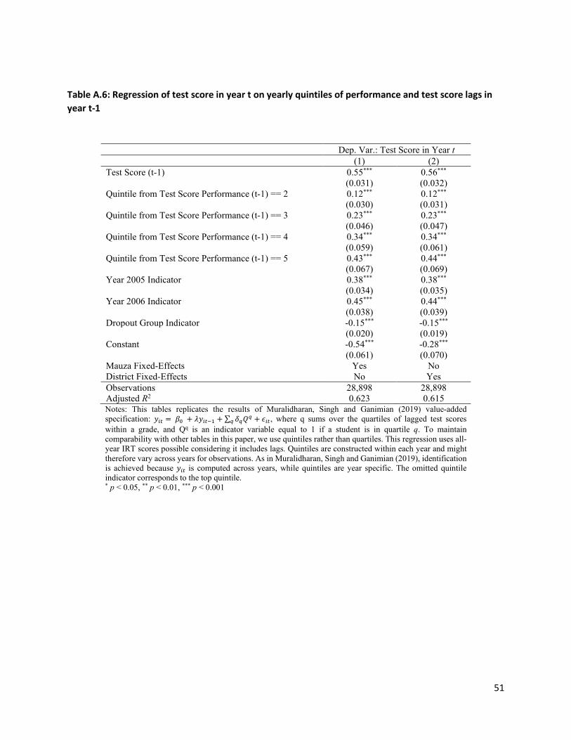
51

Table A.6: Regression of test score in year t on yearly quintiles of performance and test score lags in year t-1

Dep. Var.: Test Score in Year t (1) (2) Test Score (t-1) 0.55*** 0.56*** (0.031) (0.032) Quintile from Test Score Performance (t-1) == 2 0.12*** 0.12*** (0.030) (0.031) Quintile from Test Score Performance (t-1) == 3 0.23*** 0.23*** (0.046) (0.047) Quintile from Test Score Performance (t-1) == 4 0.34*** 0.34*** (0.059) (0.061) Quintile from Test Score Performance (t-1) == 5 0.43*** 0.44*** (0.067) (0.069) Year 2005 Indicator 0.38*** 0.38*** (0.034) (0.035) Year 2006 Indicator 0.45*** 0.44*** (0.038) (0.039) Dropout Group Indicator -0.15*** -0.15*** (0.020) (0.019) Constant -0.54*** -0.28*** (0.061) (0.070) Mauza Fixed-Effects Yes No District Fixed-Effects No Yes Observations 28,898 28,898 Adjusted R2 0.623 0.615 Notes: This tables replicates the results of Muralidharan, Singh and Ganimian (2019) value-added specification: 𝑦𝑦𝑖𝑖𝑡𝑡 = 𝛽𝛽0 + 𝜆𝜆𝑦𝑦𝑖𝑖𝑡𝑡−1 + ∑ 𝛿𝛿𝑞𝑞𝑄𝑄𝑞𝑞 + 𝜖𝜖𝑖𝑖𝑡𝑡𝑞𝑞 , where q sums over the quartiles of lagged test scores within a grade, and Qq is an indicator variable equal to 1 if a student is in quartile q. To maintain comparability with other tables in this paper, we use quintiles rather than quartiles. This regression uses all-year IRT scores possible considering it includes lags. Quintiles are constructed within each year and might therefore vary across years for observations. As in Muralidharan, Singh and Ganimian (2019), identification is achieved because 𝑦𝑦𝑖𝑖𝑡𝑡 is computed across years, while quintiles are year specific. The omitted quintile indicator corresponds to the top quintile. * p < 0.05, ** p < 0.01, *** p < 0.001

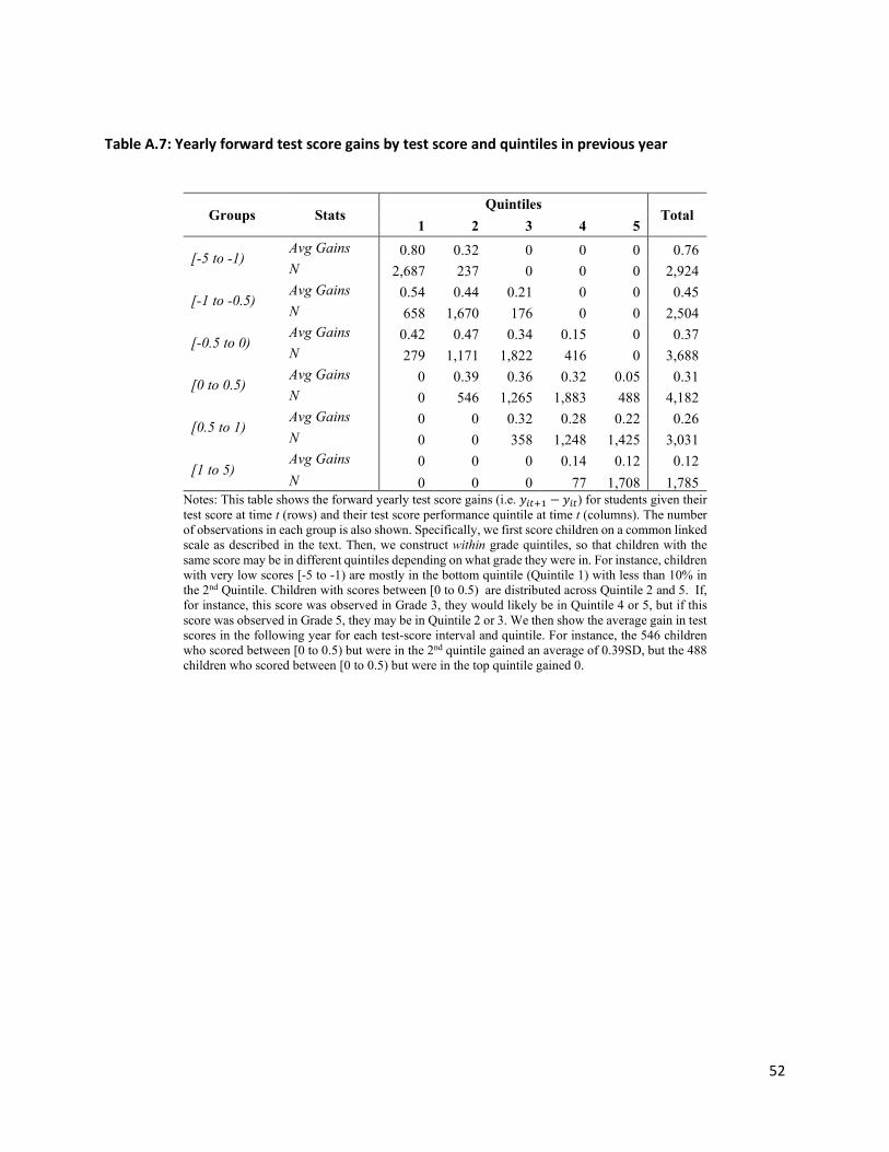
52

Table A.7: Yearly forward test score gains by test score and quintiles in previous year

Groups Stats Quintiles

Total 1 2 3 4 5

[-5 to -1) Avg Gains 0.80 0.32 0 0 0 0.76 N 2,687 237 0 0 0 2,924

[-1 to -0.5) Avg Gains 0.54 0.44 0.21 0 0 0.45 N 658 1,670 176 0 0 2,504

[-0.5 to 0) Avg Gains 0.42 0.47 0.34 0.15 0 0.37 N 279 1,171 1,822 416 0 3,688

[0 to 0.5) Avg Gains 0 0.39 0.36 0.32 0.05 0.31 N 0 546 1,265 1,883 488 4,182

[0.5 to 1) Avg Gains 0 0 0.32 0.28 0.22 0.26 N 0 0 358 1,248 1,425 3,031

[1 to 5) Avg Gains 0 0 0 0.14 0.12 0.12 N 0 0 0 77 1,708 1,785

Notes: This table shows the forward yearly test score gains (i.e. 𝑦𝑦𝑖𝑖𝑡𝑡+1 − 𝑦𝑦𝑖𝑖𝑡𝑡) for students given their test score at time t (rows) and their test score performance quintile at time t (columns). The number of observations in each group is also shown. Specifically, we first score children on a common linked scale as described in the text. Then, we construct within grade quintiles, so that children with the same score may be in different quintiles depending on what grade they were in. For instance, children with very low scores [-5 to -1) are mostly in the bottom quintile (Quintile 1) with less than 10% in the 2nd Quintile. Children with scores between [0 to 0.5) are distributed across Quintile 2 and 5. If, for instance, this score was observed in Grade 3, they would likely be in Quintile 4 or 5, but if this score was observed in Grade 5, they may be in Quintile 2 or 3. We then show the average gain in test scores in the following year for each test-score interval and quintile. For instance, the 546 children who scored between [0 to 0.5) but were in the 2nd quintile gained an average of 0.39SD, but the 488 children who scored between [0 to 0.5) but were in the top quintile gained 0.

53

Table A.8: Correlates variables definitions

Variable Variable Name Definition Asset Index (School-level data)

sc_pca_4years Predicted first Principal Component index scaled to have mean 0 across all years. It uses assets collected from a random sample of children at each school. The PCA uses assets data from 2003-06.

Assets Index (HH-level data)

hh_pca_4years Predicted first Principal Component index scaled to have mean 0 across all years. It uses assets collected at the household. The PCA uses assets data from 2003-06.

Mother Education Groups (School-level data)

sc_mother_educ Mean of available parental education groups in 2003-06 at the school-level. Missings are ignored to estimate the mean, and results are rounded to the closest unit. Parental groups follow this definition: 1 = No Education 2 = Less than Primary (less than Grade 5 - did not pass Grade 5 exams) 3 = Greater than Primary to Higher Secondary (greater or equal than Grade 5 to less or equal than Grade 12) 4 = Higher Secondary or higher (greater than Grade 12)

Father Education Groups (School-level data)

sc_father_educ

Mother Education Groups (HH-level data)

hh_mother_educ First, years of parental education is defined as the average across all observed years (ignoring missings) of the highest grade of formal schooling completed by each parent. When above 12, the following assumptions are made: (i) BA/BSC/B.Ed = 15; and (ii) MA/MSC/M.Ed/MBA = 17. Then, these parental education groups are constructed from years of parental education using the following definition: 1 = No Education 2 = Less than Primary (less than Grade 5 - did not pass Grade 5 exams) 3 = Greater than Primary to Higher Secondary (greater or equal than Grade 5 to less or equal than Grade 12) 4 = Higher Secondary or higher (greater than Grade 12)

Father Education Groups (HH-level data)

hh_father_educ

Test Items eng_item* math_item* urdu_item*

Each variable assumes that unanswered questions that were asked are marked as wrong. Only typos (i.e. values different than 0 for incorrect and 1 for correct) are set to missing if the question was asked. Variables take the value of missing if question is NOT asked in a given year.

54

Figure A.1: Vertical equating by subject

Notes: This figure shows the results of a vertical equating exercise. First, item parameters from year 1 only are estimated. Then, the item parameters are assumed to be fixed and used to re-estimate new θ’s for children using their patterns of responses for common items in year 4. The solid line in each graph is the item characteristic/response curve, which represents the expected patterns of responses for each θ. The actual patterns of responses against θ for 40 quantiles is then plotted against it. If the expected and actual patterns of responses match, this implies that children are moving along a fixed item characteristic curve and that the curve itself is not shifting across years. For 9/24 English questions, the Pearson’s Chi2 test of differences is significant between the observed and expected frequencies of answering correctly when dividing the sample in 1,000 quantiles by subject theta for a total sample of 10,067 or about 10 students by quantile.

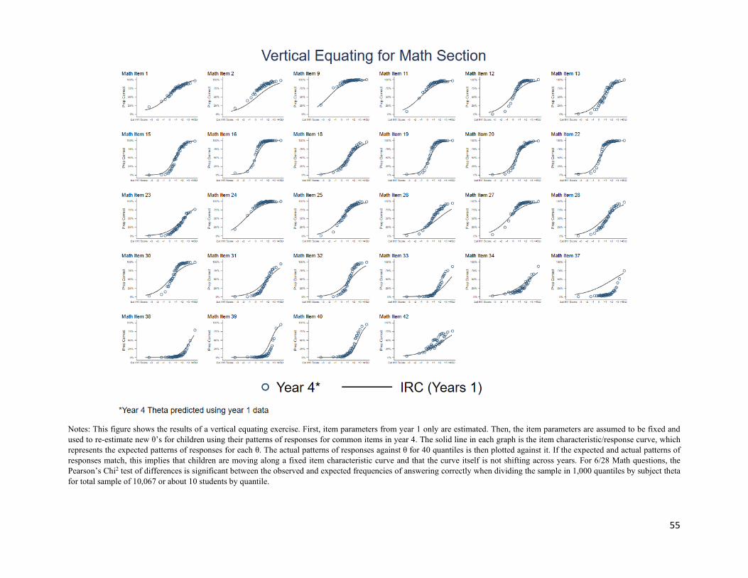
55

Notes: This figure shows the results of a vertical equating exercise. First, item parameters from year 1 only are estimated. Then, the item parameters are assumed to be fixed and used to re-estimate new θ’s for children using their patterns of responses for common items in year 4. The solid line in each graph is the item characteristic/response curve, which represents the expected patterns of responses for each θ. The actual patterns of responses against θ for 40 quantiles is then plotted against it. If the expected and actual patterns of responses match, this implies that children are moving along a fixed item characteristic curve and that the curve itself is not shifting across years. For 6/28 Math questions, the Pearson’s Chi2 test of differences is significant between the observed and expected frequencies of answering correctly when dividing the sample in 1,000 quantiles by subject theta for total sample of 10,067 or about 10 students by quantile.

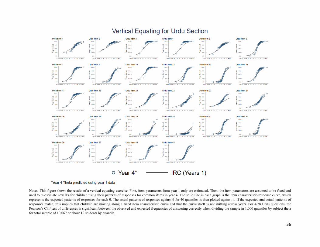
56

Notes: This figure shows the results of a vertical equating exercise. First, item parameters from year 1 only are estimated. Then, the item parameters are assumed to be fixed and used to re-estimate new θ’s for children using their patterns of responses for common items in year 4. The solid line in each graph is the item characteristic/response curve, which represents the expected patterns of responses for each θ. The actual patterns of responses against θ for 40 quantiles is then plotted against it. If the expected and actual patterns of responses match, this implies that children are moving along a fixed item characteristic curve and that the curve itself is not shifting across years. For 4/28 Urdu questions, the Pearson’s Chi2 test of differences is significant between the observed and expected frequencies of answering correctly when dividing the sample in 1,000 quantiles by subject theta for total sample of 10,067 or about 10 students by quantile.

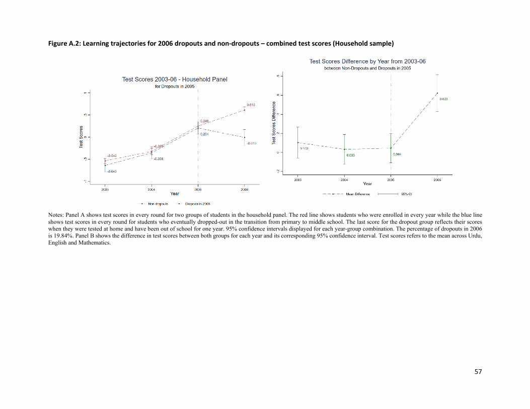
57

Figure A.2: Learning trajectories for 2006 dropouts and non-dropouts – combined test scores (Household sample)

Notes: Panel A shows test scores in every round for two groups of students in the household panel. The red line shows students who were enrolled in every year while the blue line shows test scores in every round for students who eventually dropped-out in the transition from primary to middle school. The last score for the dropout group reflects their scores when they were tested at home and have been out of school for one year. 95% confidence intervals displayed for each year-group combination. The percentage of dropouts in 2006 is 19.84%. Panel B shows the difference in test scores between both groups for each year and its corresponding 95% confidence interval. Test scores refers to the mean across Urdu, English and Mathematics.

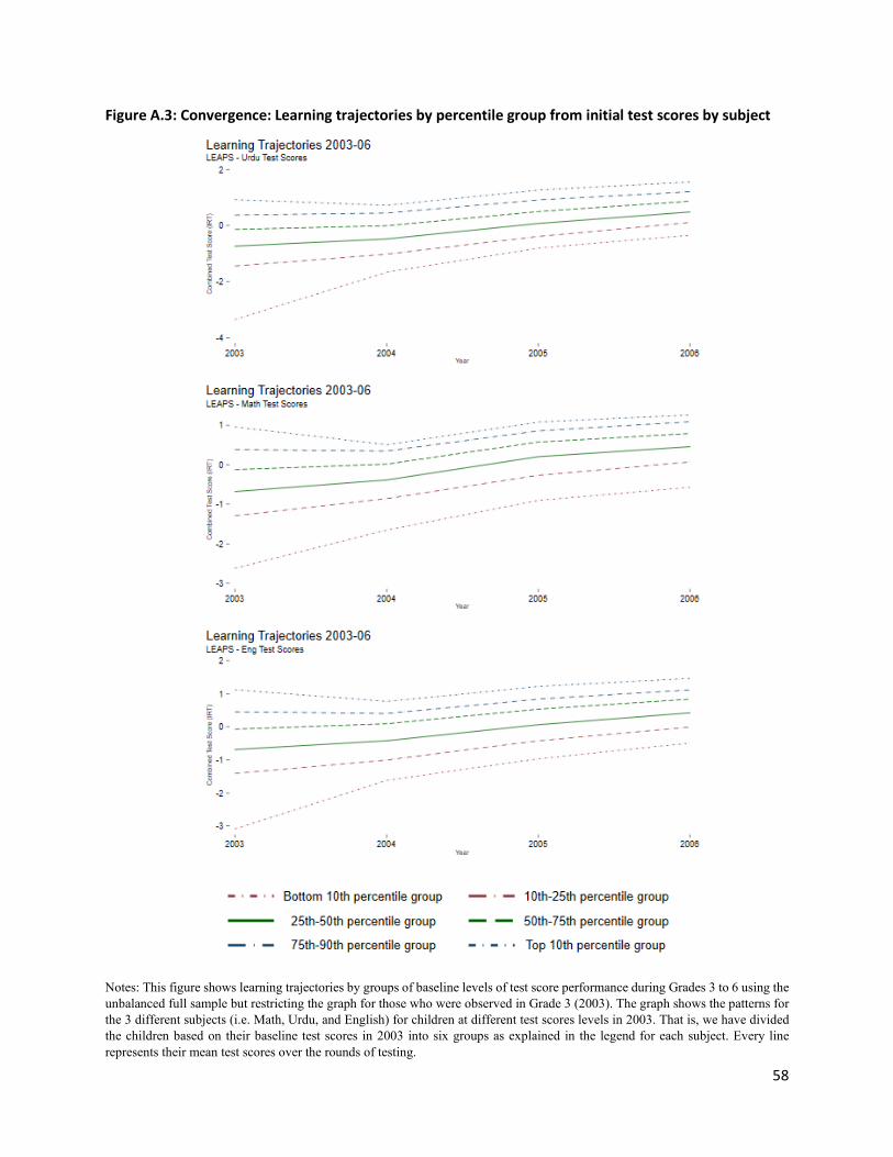
58

Figure A.3: Convergence: Learning trajectories by percentile group from initial test scores by subject

Notes: This figure shows learning trajectories by groups of baseline levels of test score performance during Grades 3 to 6 using the unbalanced full sample but restricting the graph for those who were observed in Grade 3 (2003). The graph shows the patterns for the 3 different subjects (i.e. Math, Urdu, and English) for children at different test scores levels in 2003. That is, we have divided the children based on their baseline test scores in 2003 into six groups as explained in the legend for each subject. Every line represents their mean test scores over the rounds of testing.

59

Figure A.4: Linear fit of 4-years gains and baseline test scores

Notes: High and low parental education groups are constructed from the maximum level of education across father and mother for each child. High education groups are those where the most educated parent has completed more than primary school, and low education groups are families where the most educated parent reports 0 years of schooling. In our data, 22% of parents fall in the first category, and 29% fall in the second category. The figure shows, for each group, 20 quantiles in each group and the corresponding linear fit using Catteneo’s (2019) binscatter command in Stata. For clarity, we have excluded 2% of the observations with test scores higher than +2 SD or lower than -3 SD. We have also reported coefficients from the value-added and the gains specification where all data are included. The value-added specification shows that children who started off at the same score in 2003 gained 0.27 SD extra if they were in “high” education households. The gains specification shows that, on average, children from high education households gained an additional 0.11 SD between Grades 3 and 6.

60

Figure A.5: Scatter plot and linear fit of household assets PCA and IRT indices

61

APPENDIX A: ATTRITION

Exploration of Attrition Patterns in the Data. To understand whether the patterns of number of students

observed for 1, 2, 3, and 4 years in Table 1 would occur under random attrition, we carried out a number

of simulations for the 3-year data. These are shown in Appendix Table 2, with detailed explanation of the

exercise in the notes to the table. We present data from three years because, in the fourth year, some of

the missing test scores could be because of higher dropouts. In these simulations, we assume that there

is some degree of absence in each year. We also assume that between 3% and 7% of children are

misclassified (i.e. classified as a new individual in the panel when, in fact, they had been observed before)

in every year.

Interestingly, it is quite hard to replicate observed patterns across the entire distribution with random

attrition. The fraction of children observed for 3 years is consistent with absence rates of 15% and

misclassification between 3% and 5%, but in this case, we should have seen fewer children with only one

observation. Alternately, parameters that correctly predict the number of children we see only once

under-predict the number of children with 3 years of data. Since we never observe test score gains for

these “sporadic” children, they are effectively eliminated from our sample—but remain an important

group of children that requires further investigation.29

Our working assumption remains that the data reflect 15% absenteeism, which may be selective, as well

as 3%- 5% misclassification in each year, which is likely to be random. To understand learning trajectories,

we can treat the data as a cross-section in every year, discarding the panel aspect of the data, and these

trajectories will be biased to the extent that absence and test score gains are correlated in these data.

Using an Intensively Tracked Sample to Characterize Bias. Suppose that in addition to the school sample,

we also have an “intensively” tracked sample where a greater fraction of children are observed for all four

years. Label the child’s “true” knowledge level in a given year as 𝑥𝑥𝑖𝑖𝑡𝑡, where i is the child and t the year so

that a child’s true learning gain is 𝑥𝑥𝑖𝑖𝑡𝑡 − 𝑥𝑥𝑖𝑖,𝑡𝑡−1 = 𝛿𝛿𝑖𝑖. We observe test scores, which are given by 𝑦𝑦𝑖𝑖𝑡𝑡 = 𝑥𝑥𝑖𝑖𝑡𝑡 +

𝜈𝜈𝑖𝑖𝑡𝑡, where 𝜈𝜈𝑖𝑖𝑡𝑡 is a random idiosyncratic error. Then, if we observe all students’ test scores, the average

29 This category of ‘sporadic’ children has not been documented in previous work. As reported in Table 2, children observed only once were more likely to be absent in the last 30 days as reported by their teacher. When looking at all the children between ages 5-15 in each household surveyed (not only those attending school), we observe that 10% of children are not observed consistently over the 4 years, with the majority of the years unobserved being attributed to household movements and migration. Thus, a combination of regular child absence rates, misclassification, differential absence rates, and household movement and migration might help explain the high rate of ‘sporadic’ children observed.

62

learning gains are an unbiased estimate of average learning 𝐸𝐸(𝛿𝛿𝑖𝑖). However, in a given year, we only

observe an individual if 𝐴𝐴𝑖𝑖 + 𝜖𝜖𝑖𝑖𝑡𝑡 > 𝑧𝑧, where 𝐴𝐴𝑖𝑖 is an individual-level, unobserved characteristic that may

be correlated with 𝛿𝛿𝑖𝑖, and 𝜖𝜖𝑖𝑖𝑡𝑡 is an individual-year idiosyncratic shock. Then, we can write the probability

of being observed as 𝐷𝐷(𝐴𝐴𝑖𝑖). The estimate of learning gains is then 𝛿𝛿 = 𝐸𝐸(𝑝𝑝(𝐴𝐴𝑖𝑖)𝛿𝛿𝑖𝑖)𝐸𝐸(𝑝𝑝(𝐴𝐴𝑖𝑖)) =

𝐶𝐶𝐶𝐶𝐶𝐶(𝑝𝑝(𝐴𝐴𝑖𝑖),𝛿𝛿𝑖𝑖)+𝐸𝐸�𝑝𝑝(𝐴𝐴𝑖𝑖)�𝐸𝐸(𝛿𝛿𝑖𝑖)𝐸𝐸(𝑝𝑝(𝐴𝐴𝑖𝑖))

= 𝐶𝐶𝐶𝐶𝐶𝐶(𝑝𝑝(𝐴𝐴𝑖𝑖),𝛿𝛿𝑖𝑖)𝐸𝐸(𝑝𝑝(𝐴𝐴𝑖𝑖))

+ 𝐸𝐸(𝛿𝛿𝑖𝑖). So, the bias in the estimate is 𝐶𝐶𝐶𝐶𝐶𝐶(𝑝𝑝(𝐴𝐴𝑖𝑖),𝛿𝛿𝑖𝑖)𝐸𝐸(𝑝𝑝(𝐴𝐴𝑖𝑖))

, and there is no

bias due to attrition if attrition is not correlated with 𝛿𝛿𝑖𝑖 (that is, 𝐶𝐶𝐷𝐷𝐶𝐶(𝐷𝐷(𝐴𝐴𝑖𝑖), 𝛿𝛿𝑖𝑖) = 0). Now we can consider

two samples where one is more intensively and one is less intensively tracked. For the more intensively

tracked sample, we can say that a student is observed if 𝐴𝐴𝑖𝑖 + 𝜖𝜖𝑖𝑖𝑡𝑡 > 𝑧𝑧 − Δ𝑧𝑧 , which can be written as 𝐴𝐴𝑖𝑖 +

Δ𝑧𝑧 + 𝜖𝜖𝑖𝑖𝑡𝑡 > 𝑧𝑧 . Then the difference in the estimates from the two samples is 𝐶𝐶𝐶𝐶𝐶𝐶(𝑝𝑝(𝐴𝐴𝑖𝑖+Δ𝑧𝑧),𝛿𝛿𝑖𝑖)𝐸𝐸(𝑝𝑝(𝐴𝐴𝑖𝑖+Δ𝑧𝑧))

-𝐶𝐶𝐶𝐶𝐶𝐶(𝑝𝑝(𝐴𝐴𝑖𝑖),𝛿𝛿𝑖𝑖)𝐸𝐸(𝑝𝑝(𝐴𝐴𝑖𝑖))

.

Note that this value is equal to 0 if 𝐶𝐶𝐷𝐷𝐶𝐶(𝐷𝐷(𝐴𝐴𝑖𝑖 + Δ𝑧𝑧), 𝛿𝛿𝑖𝑖) = 𝐶𝐶𝐷𝐷𝐶𝐶(𝐷𝐷(𝐴𝐴𝑖𝑖), 𝛿𝛿𝑖𝑖) = 0 (that is, if there is no

selection bias) but otherwise it is not equal to 0. Additionally, if we are willing to assume

𝐶𝐶𝐷𝐷𝐶𝐶(𝐷𝐷(𝐴𝐴𝑖𝑖 + Δ𝑧𝑧), 𝛿𝛿𝑖𝑖) ≈ 𝐶𝐶𝐷𝐷𝐶𝐶(𝐷𝐷(𝐴𝐴𝑖𝑖), 𝛿𝛿𝑖𝑖) , we note that the difference between the two estimates will be

strictly increasing in the size of the bias.

Stability of Results across Samples with Different Degrees of Attrition. Appendix Table 4 compares learning

for three different samples —a balanced sample of 6,038 children who were present in every year, the

unbalanced samples of children present in different years, and the household sample where the balanced

proportion is higher. Again, test score gains are very similar across all three samples. There are statistically

significant differences between the unbalanced/balanced panels when comparing against the household

panel but only when learning includes year 4, which is likely caused by the inclusion of testing dropouts

at home and the fact that the balanced panel itself is a (slightly) selected group of children. However,

these differences are small in magnitude (less than 0.06 SD) and suggest that absences can be treated as

equivalent to “missing at random” (with respect to learning gains) for our computations.

63

APPENDIX B: COMPARISON OF GAINS AND VALUE-ADDED SPECIFICATIONS

Instead of a gains specification, Muralidharan, Singh and Ganimian (2019) use a value-added specification

to test whether test scores converge or diverge in their sample. They run the regression 𝑦𝑦𝑖𝑖𝑡𝑡 = 𝛽𝛽0 +

𝜆𝜆𝑦𝑦𝑖𝑖𝑡𝑡−1 + ∑ 𝛿𝛿𝑞𝑞𝑄𝑄𝑞𝑞 + 𝜖𝜖𝑖𝑖𝑡𝑡𝑞𝑞 , where q sums over the quartiles of lagged test scores within a grade, 𝑄𝑄𝑞𝑞 is an

indicator variable equal to 1 if a student is in quartile q, and as in the main text 𝑦𝑦𝑖𝑖𝑡𝑡 is the test score for a

student i in a year t. Identification is achieved because 𝑦𝑦𝑖𝑖𝑡𝑡−1 is computed across grades, while quartiles

are grade specific. They show that the estimated coefficient on the lowest quartile is approximately 0.

When children at the same score are in a lower quartile because they are in a higher grade, their gains are

lower. This specification relies on the assumption that 𝜆𝜆 is a global parameter with constant effects across

quartiles and grades. When we replicate their specification in Appendix Table 6, we find evidence of

divergence, in line with their findings in India. We note, however, that assuming a constant value of the

persistence parameter 𝜆𝜆 is itself problematic. If we instead use a non-parametric table, where we simply

examine grades by test-score and quartiles (again, quartiles for the same test score are different because

children are in different grades), we find similar patterns of convergence as we have documented before

(see Appendix Table 7).