Littoral 2002, 22-26 September. Porto, Portugal

Shoreline Change due to Nearshore Dredging

Paul A. Work1, George Voulgaris2 and Fairlight Fehrenbacher3

1Assoc. Prof. and 3Grad. Res. Asst., Georgia Tech Regional Engineering Program, 6001 Chatham Center Drive, Suite 350, Savannah, GA 31405 USA. paul.work@gtrep.gatech.edu

2Asst. Prof., Marine Science Program, Dept. of Geological Sciences, Univ. of South Carolina, Columbia, SC 29208 USA. gvoulgaris@geol.sc.edu

Abstract

A methodology for assessment of impacts of nearshore dredging (for beach nourishment or other purposes) on long-term, longshore sediment transport in the surf zone is presented. The approach employs numerical model results describing mean currents (tidal and wind-induced) and wind waves and swell. The site considered is Folly Island, South Carolina, USA. Wave model results are compared to short-term measurements at three locations at the site for validation. Results indicate that wave energy dissipation is not negligible outside of the surf zone, and energy inputs by wind must also be included. Given an initial bathymetry and start time, tidal stage and velocity fields are computed, and a wind-induced velocity added based on empirical correlation between measured flows and wind speeds. Hindcast results define wave inputs, and snapshots of the wave field and longshore sediment transport rates are computed. This procedure is repeated to determine long-term shoreline change.

1. INTRODUCTION Beach nourishment is, in many locations, the only feasible or permitted means of mitigating long-term erosion problems. After identifying a nearby source of suitable sand, the impacts of moving that sand must be considered – impacts ranging from disturbance of benthic habitat to changes in nearshore waves, currents, and sediment transport.

Modifications to nearshore bathymetry can lead to several important influences on nearby beaches. If the bathymetric modifications occur in a region with depths less than half of a wavelength, wave transformation processes (primarily refraction and shoaling) will lead to modifications in the nearshore wave field (thus the term nearshore is used here to denote regions with depths less than half of a wavelength). Nearshore currents can likewise be altered by bathymetric changes, and current-induced wave refraction changed as a result.

Sediment transport that occurs subsequent to dredging can lead to infilling of the dredge pit. This can modify spatial distributions of waves and currents and can also represent a sediment sink for the littoral system.

Because of the complexities and interactions associated with the processes described above, numerical models represent the most feasible study approach. Site-specific forcing conditions must also be described. This study focuses on alterations of nearshore coastal processes due to bathymetric changes resulting from dredging for beach nourishment materials. Project volumes are often 106-107 m3.

Numerical models for wave transformation (SWAN, Booij et al. 1999) and currents (ADCIRC, Scheffner and Carson, 2001) are being used to quantify post-dredging changes in nearshore sediment transport patterns at Folly Island, South Carolina, USA (Figure 1).

Figure 1. Site location map. The site is on the southeastern (Atlantic) coast of the U.S.A.

Wave model results are validated by comparison to short-term, non-directional wave measurements, and predicted longshore gradients of longshore sediment transport are being compared to observed changes in existing beach profile data. Despite the focus on a particular site, the approach is general in that it can be applied to other sites and will reveal suitability of offshore borrow sites for beach nourishment material, from a hydrodynamic standpoint.

1

Littoral 2002, 22-26 September. Porto, Portugal

2. INPUT DATA AND FIELD MEASUREMENTS The SWAN wave transformation model (Booij et al. 1999) requires description of bathymetry, water levels, mean flows, and winds throughout the domain, and incident waves on all model boundaries (described in spectral terms, i.e. energy as a function of frequency and direction). Unfortunately, field measurements to describe these parameters are limited or unavailable at many sites, including the one considered here. Thus predicted values (derived from wave hindcasts) must often be relied upon.

The following relevant data sources are available and employed here:

- Digital bathymetry (National Geodetic Data Center, Sharman et al. 1998).

- U.S. Army Corps of Engineers WIS Wave Hindcast Data (1976-95, 9 m depth, Brooks and Brandon 1995).

- Short-term (two months) measurements of mean currents and waves, 2 km offshore of Folly Island (Jin 2001; see Figure 2).

- Predictions (via numerical model) of currents in area (Scheffner and Carson 2001).

- Measured beach profile data, typically biannual, since the early 1980’s.

- Long-term (1984-present) measurements of gust, 2-min (hourly) and 10-min (continuous) wind speeds at the northern end of Folly Island.

Unfortunately the only available long-term (1994-present) wave measurements are recorded 75 km remote to the study site and no longer include directional characteristics of the waves. Thus the wave hindcast data are best suited for making long-term predictions.

The short-term field measurements will be considered first to assess site characteristics and suitability of the wave transformation model.

A Sontek Argonaut-XR acoustic current meter was deployed twice, roughly 2 km offshore of Folly Island (Figure 2), yielding data describing waves and currents at the site during one summer month (June 1998) and one winter month (December 1998-January 1999). Measured parameters include water depth, non-directional wave energy spectra, and mean flow speeds representing water column averages. Jin (2001) provides details of the data set omitted here.

Figure 2. Detail of site showing location of three instruments. “+C” denotes location of Sontek current meter/non-directional wave gauge, “W1” and “W2” show locations of non-directional wave gauges built by author.

Harmonic analysis indicated that 97% (summer) and 95% (winter) of the water level fluctuations were attributable to tidal forcing. Thus predicted tides yield a suitable description of water levels for all but extreme events.

Flows were observed to rotate through the tidal cycle, and flows in the longshore direction dominated except when a strong cross-shore wind component existed. Tidal forcing is attributable for 86% (summer) and 63% (winter) of the cross-shore flows, and 68% (summer) and 44% (winter) of the longshore flows. The direction of each component of the mean flow reverses by season. Mean flows are northeastward in summer and southwestward in winter (Figure 3). This is attributed to changes in the mean wind stress vector between the two seasons (Blanton et al. 1985).

Figure 3. Measured mean longshore and cross-shore flows by season for two deployments: Summer (6/1/98-7/2/98) and Winter (12/9/98-1/15/99). Bathymetric contours at 2 m interval also shown.

Residual longshore and cross-shore currents were computed for both deployment periods (“residual” denoting the difference between measured and predicted tidal currents, using

2

Littoral 2002, 22-26 September. Porto, Portugal

results from harmonic analysis of the measurements). Figure 4 shows results for the summer deployment period. Longshore flows were similarly dominant in the winter data set, but with the mean flow in the opposite direction. Residual longshore flows in both seasons are correlated with longshore wind stress (Figure 5). Residual cross-shore flows were not correlated with cross-shore winds, except for the case of very strong onshore winds.

Figure 4. Longshore and cross-shore mean (top) and residual flows (bottom) for summer ’98 deployment. In each case, solid line is longshore flow (positive is to NE), dotted lines denote cross-shore flow (positive denotes onshore).

Figure 5. Residual longshore (top) and cross-shore (bottom) currents vs. longshore and cross-shore 2-min wind vectors. Winter ’98-99; results similar for summer deployment. Line denotes best fit (least squares) in each case.

A finite difference representation of the bathymetry (188 x 171 nodes, ∆x = 149 m, ∆y = 50 m, depth ~9 m on seaward boundary) was generated for the study area using data from the National Geodetic Data Center. For specification of mean flows within the SWAN model, it was necessary to determine mean currents at each

node within the grid; these are provided as input to the wave model.

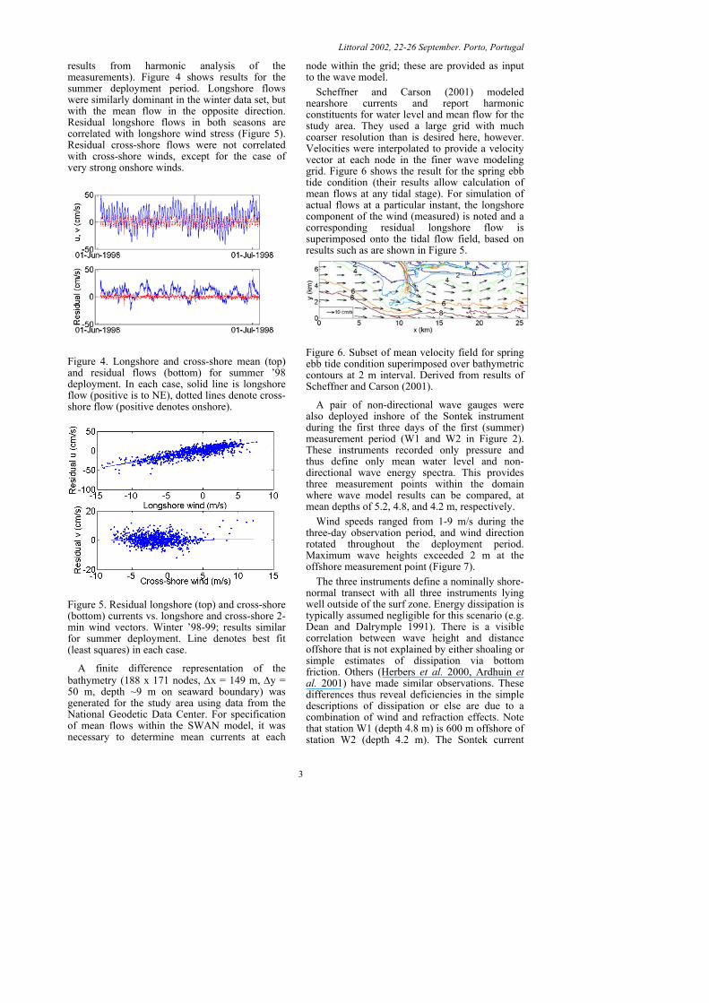
Scheffner and Carson (2001) modeled nearshore currents and report harmonic constituents for water level and mean flow for the study area. They used a large grid with much coarser resolution than is desired here, however. Velocities were interpolated to provide a velocity vector at each node in the finer wave modeling grid. Figure 6 shows the result for the spring ebb tide condition (their results allow calculation of mean flows at any tidal stage). For simulation of actual flows at a particular instant, the longshore component of the wind (measured) is noted and a corresponding residual longshore flow is superimposed onto the tidal flow field, based on results such as are shown in Figure 5.

Figure 6. Subset of mean velocity field for spring ebb tide condition superimposed over bathymetric contours at 2 m interval. Derived from results of Scheffner and Carson (2001).

A pair of non-directional wave gauges were also deployed inshore of the Sontek instrument during the first three days of the first (summer) measurement period (W1 and W2 in Figure 2). These instruments recorded only pressure and thus define only mean water level and non-directional wave energy spectra. This provides three measurement points within the domain where wave model results can be compared, at mean depths of 5.2, 4.8, and 4.2 m, respectively.

Wind speeds ranged from 1-9 m/s during the three-day observation period, and wind direction rotated throughout the deployment period. Maximum wave heights exceeded 2 m at the offshore measurement point (Figure 7).

The three instruments define a nominally shore-normal transect with all three instruments lying well outside of the surf zone. Energy dissipation is typically assumed negligible for this scenario (e.g. Dean and Dalrymple 1991). There is a visible correlation between wave height and distance offshore that is not explained by either shoaling or simple estimates of dissipation via bottom friction. Others (Herbers et al. 2000, Ardhuin et al. 2001) have made similar observations. These differences thus reveal deficiencies in the simple descriptions of dissipation or else are due to a combination of wind and refraction effects. Note that station W1 (depth 4.8 m) is 600 m offshore of station W2 (depth 4.2 m). The Sontek current

3

Littoral 2002, 22-26 September. Porto, Portugal

meter (depth 5.2 m) is another 700 m offshore of station W1.

Figure 7. 10-min wind speeds (top) measured at Folly Island C-MAN station and wave heights (bottom) for the three simultaneously deployed instruments.

The wave model was run for one case (6/30/98, 22:30 GMT) using only measured winds as a source of input energy (i.e. no incident waves). In this instance, the wind was nominally shore-parallel, and waves build as they approach Stono Inlet shoals (on west end of Folly Island), then break, and re-form (Figure 8). The simulation represents a steady state solution; downwind of Stono Inlet shoals, waves become limited by fetch, and gradually increase in height with distance from the shoals.

Figure 8. Wave height contours for 7.2 m/s wind from 220 degrees (left boundary). Conditions correspond to measured winds, water level, 6/30/98 22:30GMT. No mean currents.

Figure 9 shows three, shore-parallel transects of model-derived wave heights and seafloor elevations, one through each wave gauge location. Differences in predicted wave heights between transects are negligible, but predicted wave

heights are less than half of measured values. Thus incident wind waves must also be prescribed along the model boundary to reproduce the field measurements. Refraction effects for this case are also similar for each measurement location – bathymetric contours are regular between the shoals and the measurement stations.

Figure 9. Longshore transects of seafloor elevation (bottom) and wave height (top) passing through each measurement location. Continuous lines are from model results; measurements also shown in top plot. 7.2 m/s wind from 220 (measured); zero wave heights on boundaries, zero currents.

The two available sources of long-term wave data are wave hindcast results (at the 9 m depth contour) and wave buoy measurements 75 km offshore (depth 37 m). Wave hindcast results are not available for the measurement period, however. In order to simulate the 1998 test cases, it is necessary to transform waves from the offshore measurement location.

The large distance (75 km) between the offshore measurements (NOAA buoy 41004, depth 37 m) and the offshore boundary of the model grid exceeds the limit of applicability of the chosen wave model. Rather than using a numerical model to transform waves from the wave buoy to the seaward boundary of the computational grid, Snell’s Law was used to determine wave direction and conservation of energy was assumed to determine wave height. Wave direction at the peak of the energy spectrum was taken as the single representative wave direction.

The directional characteristics of the offshore measurements and the hindcast data are compared, for the two-year (1994-95) period for which they overlap, in Figure 10. Each offshore measurement was transformed to the 9 m depth contour (corresponding to the depth of the

4

Littoral 2002, 22-26 September. Porto, Portugal

hindcast station near the site) using linear wave theory (assuming conservation of energy) and compared to the hindcast result. Maximum and mean values of the difference in monthly mean direction are 5.6 and 0.2 degrees, respectively.

0

0.5

1

1.5

2

1 3 5 7 9 11 ALLMonth

Mea

n H

mo

(m)

NOAAWIS 35

Figure 11. Mean wave heights by month for offshore measurements (NOAA Station 41004, after transformation to 9 m depth contour) and WIS hindcast (Station 35).

Mean wave heights are within 5% of one another for each month (Figure 11). Thus it is concluded that in an average sense, use of either the hindcast data or offshore measurements transformed to an equivalent depth will yield similar descriptions of incident wave height and direction over the long term.

The shape of the incident wave spectrum is a remaining problem. The WIS hindcast data do not include a description of the shape of the directional spectrum, and the shape of the spectrum reported at the offshore measurement location will change as the waves approach the coast. Thus it was elected to use an empirical, parameterized approach to describe the shape of the incident wave energy spectrum, as a function of wave height, mean direction, and two parameters describing the degree of spreading along the direction and frequency axes. A cosine-squared directional distribution was assumed.

In this fashion, incident waves at the seaward boundary of the computational grid were determined for the test case including measurements. The results significantly underestimate wave heights at the measurement locations, however. The incident wave height at the seaward boundary was then increased incrementally in an attempt to reproduce the measurements. After more than doubling the wave height at the offshore boundary, the result shown in Figure 12 is obtained. Figure 13 indicates spatial variations in wave height for the same case.

050

100150200

1 4 7 10 ALLMonth

Mea

n w

ave

dir

(deg

rees

)

NOAAWIS 35

Figure 10. Mean wave direction by month for offshore measurements (NOAA Station 41004, after transformation to 9 m depth contour) vs. WIS hindcast results, 1994-95 (Station 35).

Figure 12. Longshore transects of seafloor elevation (bottom) and wave height (top) passing through each measurement location. Continuous lines are from model results; measurements also shown in top plot. 7.2 m/s wind from 220 (measured 6/30/98 22:30GMT) plus 2.2 m wave height on seaward boundary; zero currents.

5

Littoral 2002, 22-26 September. Porto, Portugal

- dissipation is significant and may not be correctly modeled with “default” parameters

Thus a wave model that does not include wind forcing will not yield realistic results for this site. The importance of wave-current interaction will vary throughout the tidal cycle, as the direction and magnitude of the mean flow vary, but should be minimized for nominally shore-normal waves, except near inlets. Mean flows propagating with or against waves either increase or decrease wavelengths, resulting in current-induced wave refraction, but this effect vanishes if the wave propagates across the current. Figure 13. Wave height contours (interval = 0.1

m) for simulation described in Figure 12. 3. WAVE MODEL SENSITIVITY TESTS The model thus reproduces the observed trend

in the measured wave heights, but the simple approach for estimation of incident waves underestimates, for the case considered here, the wave heights at the seaward boundary of the model grid. Energy sources and sinks between the offshore measurement point and the offshore model boundary are the most likely explanation.

The processes being modeled are highly nonlinear and controlled by a large number of input variables: tidal stage (which controls tidal currents), incident waves (with associated height, period, direction, and frequency and directional distributions), wind speed and direction, and bathymetry. All of these inputs are time-dependent, although the bathymetry is often assumed slowly varying or steady, and will be assumed steady here.

The simple approach used to transform the waves from the offshore measurement buoy to the offshore boundary of the computational grid neglects any changes in wave energy due to wind or dissipation within the bottom boundary layer between the two locations. This problem is removed when using the wave hindcast data, however, since the hindcast data are reported at the 9 m contour and there is no need to transform from deep water.

Some sensitivity tests have been performed to assess the significance of any errors or uncertainty in any of the input parameters. The first to be addressed is the mean velocity field.

Waves propagating against or with a current will be shortened or stretched, respectively. This effect vanishes as the angle between the waves and currents approaches 90 degrees (i.e. waves crossing a current). The model appears to overestimate dissipation

near the offshore boundary of the domain, and then underestimate the rate of dissipation in the interior of the domain. The characteristics of the dissipation may be adjusted via empirical parameters; this will be investigated as a means to improve model realism. Herbers et al. (2000) required a friction factor of 0.1 – much larger than commonly employed – to describe observed energy dissipation, attributing this enhanced dissipation to bedforms.

Per Figure 6 (and others), the mean currents at the site are nearly shore-parallel, except near the tidal inlets. Thus wave-current effects are not expected to dominate except perhaps near the inlets. Since the focus here is on surf zone sediment transport, breaking wave heights will be taken as the primary basis for comparison when making analyses of model sensitivity.

Breaking wave heights and breaking points in a spectral model are not well defined. A ratio of wave height to water depth of 0.5 was somewhat arbitrarily taken to indicate the location of the break point within the model. In reality there is no “point” at which breaking occurs, but rather a region with poorly defined boundaries.

To summarize the findings based on interpretation of the field measurements and the comparison to model results presented here:

- tidal predictions yield suitable estimates of water levels at the site,

- superposition of a wind-driven longshore current on top of the tidal flow explains much of the variation in the longshore flow

The breaking wave heights will be used to quantify longshore sediment transport rates, which are an important control on long-term erosion or deposition and thus make a good basis for comparison. This method does not work well close to an inlet, however, where sediment transport may be controlled largely by mean

- wind wave effects are significant at times

6

Littoral 2002, 22-26 September. Porto, Portugal

flows. Thus the use of breaking wave heights for comparison of model results will be limited to those regions not immediately adjacent to an inlet or sheltered by an ebb tidal shoal. This implies excluding about 20% of the Folly Island shoreline from comparison.

A single parameter was employed to quantify differences between two model simulations, based on computed wave heights:

( )

i

jiji

HIHH

∑−

=

2',,

ε (1)

where = the value of computed wave height

at model node i,j, is the corresponding value for the other model result under consideration, and is in the incident wave height on the seaward boundary.

jiH ,', jiH

iH

Figure 14. Influence of mean current on wave heights. x-axis indicates strength of ebb tidal current, y-axis defined by Eqn. (1). Normally incident waves; Hmo = 1.6 m, Tp = 5.4 s.

The mean tide range at the site is 1.6 m. Tidal stage is represented in the model by adding a constant to all depths within the domain (i.e. domain is assumed small compared to tidal wavelength). Wave heights within the domain are only weakly affected by changes in tidal stage, except where the tidal amplitude is large compared to the mean depth, i.e. within the surf zone and near tidal shoals. Thus for the purposes of predicting surf zone sediment transport rates, it is important to resolve water level changes due to tides. Tidal stages are well described, and easily described, by predictions derived from harmonic analysis, however, so this issue will not be considered further.

Figure 14 shows the dependence of the parameter ε on the strength of the ebb tidal current. Two comparisons are made: one involves comparing wave heights everywhere within the domain, whereas the other compares only breaking wave heights along the shoreline of Folly Island (only areas not sheltered by shoals). The first comparison (asterisks) involves averaging over many more points, including many that are negligibly affected by the mean currents. Root-mean-square wave height changes are less than 3% for currents even three times greater than actually encountered at the site. Wind exerts a significant influence on the

model results, but is easily included. It will be assumed that winds are uniform over the domain, since no data are available to indicate otherwise.

When only breaking waves are used as the basis for comparison, the relative influence of the currents is stronger. Realistic mean flows modify the breaking wave heights by 2.5% on a root-mean-square basis; for stronger currents, up to 5% changes are evident. For long-term sediment transport predictions, inclusion of mean currents is important, but the currents do not influence the breaking wave heights as much as bathymetry or large changes in tidal stage.

Obviously the wave model results are quite sensitive to the description of the incident waves, including not only wave height, period and direction, but also the directional distribution and the degree of spreading along the frequency axis of the energy spectrum. Since nearshore directional spectra are not available, however, parameterized spectra have been employed (i.e. JONSWAP spectrum with cos2 directional distribution).

4. DREDGE PIT SPECIFICATION AND INFLUENCE Gayes et al. (1998) identified two potential borrow sites near Folly Island (Figure 15). One site includes an estimated 540,000 m3 of medium quality sand and is located 4-8 km offshore of Folly Island (marked “A” in Figure 15). The other is Stono Inlet shoals (“B”), where 1.5 million m3

7

Littoral 2002, 22-26 September. Porto, Portugal

where Q denotes total longshore sediment transport rate (volume/time) and x is the longshore coordinate. A positive value for this derivative indicates shoreline erosion and a negative value denotes accretion.

of low quality sand was identified. Both are being considered as a part of the research described here.

Figure 17 provides an example of results for three different sets of conditions. Each represents a snapshot, since wave conditions are constant for each simulation. The three simulations include cases with and without ebb tidal currents and with and without a dredge pit. The presence of the dredge pit is seen to exert a negligible impact on the shoreline change, but the current does modify the picture, particularly near Stono Inlet. At a few points, even the sign (erosion vs. accretion) is changed due to the presence of the current.

Figure 15. Two of the potential borrow pit areas identified by Gayes et al. (1998). Bathymetric contours at 2 m interval.

Several different dredge pit configurations are being tested. As an example, one scenario includes a pit with a square footprint 1 km x 1 km in planform, and a 2 m depth, for a volume of 2 million m3. Figure 16 shows this simulated post-dredge bathymetry.

Figure 17. Longshore gradient of longshore sediment transport vs. longshore coordinate for three different simulations: 1) zero current, no dredge pit, 2) maximum ebb current, no dredge pit, 3) zero current, dredge pit included. All cases: zero tide stage, Hmo=1.6 m, Tp = 5.4 s, normally incident waves. Figure 16. Model bathymetry including 2 million

m3 dredge pit at seaward end of Stono Inlet shoals (box).

The large positive value appearing in Figure 17 at x = 20 km corresponds to the location of a long-term erosion problem area referred to by locals as “The Washout”. It also lies in the lee of a persistent shoal – Figure 18 shows that this shoal existed even as early as 1858. The shoreline orientation changes in the lee of this shoal, which, combined with the influence of the shoal on wave heights and directions, leads to a positive longshore gradient of longshore sediment transport, i.e. an erosional zone, at least for the wave conditions used here.

The ultimate goal here is to investigate changes in longshore sediment transport patterns, which yield shoreline changes. Given a wave model result, breaking wave heights are computed, and then longshore sediment transport rates evaluated using the “CERC Equation,” which relates total (i.e. integrated across the surf zone) longshore sediment transport rate to the longshore component of wave power (energy flux).

The longshore sediment transport rate is evaluated for each computational node along the shoreline of the island, and then the longshore gradient of the longshore sediment transport rate approximated as

A large suite of simulations will be required to prove conclusively that the change in shoreline orientation and the presence of the shoal shown in Figure 18 are the cause of the long-term erosion problem at “The Washout”. The influence of the shoal on nearshore wave conditions is evident even in simulations with small incident wave heights, however (Figure 19). x

QdxdQ

∆∆

≈ (2)

8

Littoral 2002, 22-26 September. Porto, Portugal

The persistence of the shoal in shallow (<6 m) depths is of interest; it may be a relict tidal deposit – the deepest part of the main channel of Charleston Harbor terminated near Lighthouse Inlet, at the north end of Folly Island, prior to construction of jetties at the harbor. Additional simulations will reveal the dependency of the erosional zone at “The Washout” on incident wave conditions, tidal currents, and tidal stage.

Figure 18. Detail from 1:30,000 scale nautical chart, showing shoal offshore of point where shoreline orientation changes on Folly Island. Source: “Preliminary Chart of Charleston Harbor and its Approaches,” 1858, Office of Coast Survey, National Ocean Service, NOAA.

Figure 19. SWAN wave model result for one pre-dredge case. Shade indicates wave height. Longshore gradients of wave height strongest near inlets (x = 10 km, x = 24 km) and at a site known as “The Washout” (x = 20 km).

5. LONG-TERM MODELING APPROACH The approach employed in this study to describe long-term (months to years) impacts of nearshore dredging relies extensively on the numerical wave

and current model results. The overall modeling approach may be outlined as follows:

1) Use existing digital bathymetry as initial condition (National Geodetic Data Center GEODAS data)

2) ADCIRC model results (Scheffner and Carson 2001) define mean flows and water levels at any stage of tide

3) U.S. Army Corps of Engineers WIS wave hindcast results define input wave conditions at 9 m contour, every three hours

Lighthouse Inlet

4) U.S. National Oceanic and Atmospheric Administration (NOAA) measurements define winds (hourly data)

5) Run SWAN model to determine a snapshot of nearshore waves

6) Compute longshore gradient of longshore sediment transport

7) Repeat for other conditions (water levels, currents, and waves), integrate in time

Shoal 8) Repeat entire methodology for different dredging scenarios

Lastly, the model results describing location and magnitude of erosional and depositional zones along the island will be compared with available beach profile data to reveal the overall efficacy of the methodology. 6. CONCLUSIONS A methodology for assessing the impacts of nearshore dredging on longshore sediment transport in the surf zone, and thus long-term shoreline change, was presented. The setting considered is a barrier island bounded by tidal inlets at each end, south of Charleston Harbor, South Carolina, USA. Although all of the results presented are site-specific, the methodology could be employed at any site in a similar setting.

The methodology relies on hindcast results to describe incident wave conditions and mean flow speeds due to tidal effects. Wind-generated longshore currents are superimposed based on empirical estimates. The flow field serves as one input to the chosen wave model. The overall methodology is comprehensive in that it includes a spectral description of incident waves, wind wave generation, nonlinear wave-wave interactions, shoaling, refraction, breaking, and wave-current interaction.

Different descriptions of dredge borrow areas are being tested. Infilling of the dredge hole is not considered; this would tend to reduce the impacts of the dredging on the adjacent beaches over time.

Littoral 2002, 22-26 September. Porto, Portugal

10

Thus the results shown here represent a worst-case situation from this perspective.

Field measurements of mean currents at the site indicate general site characteristics and yield a relationship between longshore winds and wind-generated longshore residual currents. Wave measurements reveal a marked decrease in wave energy flux as the waves approach shore. The wave model reproduces this trend to some degree.

Short-term simulations reproduce longshore sediment transport patterns consistent with a long-term erosional feature in the lee of a persistent shoal at the site. The persistence of the erosional feature is hypothesized to be due to the presence of the shoal and a change in shoreline orientation that is observed at this location. Additional simulations will reveal any wave conditions that reverse this trend and the impact of proposed dredging activities on the entire shoreline of the island.

ACKNOWLEDGEMENT

This work is supported by the South Carolina Sea Grant Consortium.

REFERENCES Ardhuin, F., Herbers, T.H.C., and O’Reilly, W.C., 2001. A hybrid Eulerian-Lagrangian model for spectral wave evolution with application to bottom friction on the continental shelf. J. Phys. Oceanography, 31(6), 1498-1516. Blanton, J.O., Schwing, F.B., Weber, A.H., Pietrafesa, L.J., and Hayes, D.W., 1985. Wind stress climatology in the South Atlantic Bight. In Oceanography of the Southeastern U.S. Continental Shelf, L.P. Atkinson et al., Eds., Coastal and Estuarine Sci. Vol. 2, Amer. Geophys. Union, Washington, DC, 10-22. Booij, N., Ris, R.C., and Holthuijsen, L.H., 1999. A third-generation wave model for coastal regions. 1. Model description and validation. J. Geophys. Res., 104(C4), 7649-7666. Brooks, R.A., and Brandon, W.A., 1995. Hindcast wave information for the U.S. Atlantic Coast: Update 1976-1993, with hurricanes. WIS Report 33, U.S. Army Corps of Engineers Waterways Expt. Station, Vicksburg, MS. Dean, R.G., and Dalrymple, R.A., 1991. Water Wave Mechanics for Engineers and Scientists. World Scientific, Singapore. Gayes, P.T., Donovan-Ealy, P., Harris, M.S., and Baldwin,W., 1998. Assessment of Beach Renourishment Resources on the Inner Shelf off Folly Beach and Edisto Island, South Carolina.

Center for Marine and Wetland Studies, Technical Report submitted to Minerals Management Service, Office of International Activities and Marine Minerals, 43 pp. plus Appendices. Herbers, T.H.C., Hendrickson, E.J., and O’Reilly, W.C., 2000. Propagation of swell across a wide continental shelf. J.Geophys. Res., 105(C8), 19729-19737. Jin, X., 2001. Nearshore wave and current measurements and prediction: Folly Beach, South Carolina. M.S. thesis, Dept. of Civil Eng., Clemson Univ., Clemson, SC. Scheffner, N.W., and Carson, F.C., 2001. Coast of South Carolina Storm Surge Study. Final Report. ERDC/CHL TR-01-11, U.S.Army Corps of Eng., Vicksburg, MS. Sharman, G., Metzger, D., Compagnoli, J., Butler, T., Berggren, T., Divins, D., and Steele, M., 1998. GEODAS: A hydro/bathy data management system. Surveying and Land Information Systems, 58(3), 141-146.