Large-Scale Spatial Distribution Patterns of Echinodermsin Nearshore Rocky HabitatsKatrin Iken1*, Brenda Konar1, Lisandro Benedetti-Cecchi2, Juan Jose Cruz-Motta3, Ann Knowlton1,

Gerhard Pohle4, Angela Mead5, Patricia Miloslavich3, Melisa Wong6, Thomas Trott7, Nova Mieszkowska8,

Rafael Riosmena-Rodriguez9, Laura Airoldi10, Edward Kimani11, Yoshihisa Shirayama12, Simonetta

Fraschetti13, Manuel Ortiz-Touzet14, Angelica Silva6

1 School of Fisheries and Ocean Sciences, University of Alaska Fairbanks, Fairbanks, Alaska, United States of America, 2 Department of Biology, University of Pisa, Pisa, Italy,

3 Departamento de Estudios Ambientales, Centro de Biodiversidad Marina, Universidad Simon Bolivar, Caracas, Venezuela, 4 Atlantic Reference Centre, Huntsman Marine

Science Centre, St. Andrews, New Brunswick, Canada, 5 Department of Zoology, University of Cape Town, Rondebosch, South Africa, 6 Bedford Institute of Oceanography,

Dartmouth, Nova Scotia, Canada, 7 Department of Biology, Suffolk University, Boston, Massachusetts, United States of America, 8 Marine Biological Association of the

United Kingdom, Plymouth, United Kingdom, 9 Centro Interdipartimentale di Ricerca per le Scienze Ambientali, University of Bologna, Ravenna, Italy, 10 Kenya Marine and

Fisheries Research Institute, Mombasa, Kenya, 11 Programa de Investigacion en Botanica Marina, Departamento de Biologia Marina, Universidad Autonoma de Baja

California Sur, La Paz, Baja California Sur, Mexico, 12 Seto Marine Biological Laboratory, Kyoto University, Wakayama, Japan, 13 Laboratorio di Zoologia e Biologia Marina,

Dipartimento di Scienze e Tecnologie Biologiche ed Ambientali, Universita del Salento, Lecce, Italy, 14 Centro de Investigaciones Marinas, Universidad de La Habana,

Miramar Playa, Ciudad de La Habana, Cuba

Abstract

This study examined echinoderm assemblages from nearshore rocky habitats for large-scale distribution patterns withspecific emphasis on identifying latitudinal trends and large regional hotspots. Echinoderms were sampled from 76 globally-distributed sites within 12 ecoregions, following the standardized sampling protocol of the Census of Marine Life NaGISAproject (www.nagisa.coml.org). Sample-based species richness was overall low (,1–5 species per site), with a total of 32asteroid, 18 echinoid, 21 ophiuroid, and 15 holothuroid species. Abundance and species richness in intertidal assemblagessampled with visual methods (organisms .2 cm in 1 m2 quadrats) was highest in the Caribbean ecoregions and echinoidsdominated these assemblages with an average of 5 ind m22. In contrast, intertidal echinoderm assemblages collected fromclearings of 0.0625 m2 quadrats had the highest abundance and richness in the Northeast Pacific ecoregions whereasteroids and holothurians dominated with an average of 14 ind 0.0625 m22. Distinct latitudinal trends existed forabundance and richness in intertidal assemblages with declines from peaks at high northern latitudes. No latitudinal trendswere found for subtidal echinoderm assemblages with either sampling technique. Latitudinal gradients appear to besuperseded by regional diversity hotspots. In these hotspots echinoderm assemblages may be driven by local and regionalprocesses, such as overall productivity and evolutionary history. We also tested a set of 14 environmental variables (sixnatural and eight anthropogenic) as potential drivers of echinoderm assemblages by ecoregions. The natural variables ofsalinity, sea-surface temperature, chlorophyll a, and primary productivity were strongly correlated with echinodermassemblages; the anthropogenic variables of inorganic pollution and nutrient contamination also contributed tocorrelations. Our results indicate that nearshore echinoderm assemblages appear to be shaped by a network ofenvironmental and ecological processes, and by the differing responses of various echinoderm taxa, making generalizationsabout the patterns of nearshore rocky habitat echinoderm assemblages difficult.

Citation: Iken K, Konar B, Benedetti-Cecchi L, Cruz-Motta JJ, Knowlton A, et al. (2010) Large-Scale Spatial Distribution Patterns of Echinoderms in Nearshore RockyHabitats. PLoS ONE 5(11): e13845. doi:10.1371/journal.pone.0013845

Editor: Simon Thrush, National Institute of Water & Atmospheric Research (NIWA), New Zealand

Received June 4, 2010; Accepted October 4, 2010; Published November 5, 2010

Copyright: � 2010 Iken et al. This is an open-access article distributed under the terms of the Creative Commons Attribution License, which permits unrestricteduse, distribution, and reproduction in any medium, provided the original author and source are credited.

Funding: We would like to express our most sincere gratitude to the Alfred P. Sloan Foundation for funding. Support from the History of the Near Shore programwas instrumental for collections in South Africa (AM), United Kingdom (NM), and Maine, USA (TT). For sampling in Maine, logistical support in the field andfinancial aid for data collection and processing was also provided by Suffolk University, Boston, Massachusetts, USA to TT. Collections at Canso, Canada weresupport by the Department of Fisheries and Oceans Canada to MS and AS. Collections at Conero Riviera, Italy were supported by the AdriaBio project (Universityof Bologna Strategic Project, 2007-2009) to LA. Support for sites in Japan was provided by the Nippon Foundation, Japan Society for Promotion of Science to YS.Funding for data collection in the Gulf of Alaska came from the Gulf Ecosystem Monitoring Program to BK and KI. Sampling in the Arctic was supported by the USMinerals Management Service to KI. The funders had no role in study design, data collection and analysis, decision to publish, or preparation of the manuscript.

Competing Interests: The authors have declared that no competing interests exist.

* E-mail: iken@ims.uaf.edu

Introduction

Biodiversity assessments in marine systems are of great interest

from ecological, public and management standpoints. They are

important for understanding ecological patterns and ecosystem

functioning and for managing marine resource use and identifying

conservation priorities [1–3]. A particular ecological interest is the

identification of large-scale biodiversity patterns to investigate

possible factors driving diversity, and to serve as context for local

ecological studies and in management and conservation [4]. It has

long been postulated that diversity in marine species or

communities may follow latitudinal gradients with diversity

peaking at the equator and declining towards higher latitudes

[5], with evolutionary, historical and ecological mechanisms

PLoS ONE | www.plosone.org 1 November 2010 | Volume 5 | Issue 11 | e13845

suggested as drivers [6]. Support for this trend is evident from

shallow waters to the deep-sea [7–10] and a recent meta-analysis

suggests that the trend can be viewed as a generalized pattern in

marine taxa [11]. Nevertheless, biodiversity in some taxa or

communities does not follow this postulated general latitudinal

gradient. While this gradient may be an overarching feature, there

are notable exceptions, e.g., in macroalgae [12–14], in benthic

soft-sediment shelf communities [14–16] and rocky intertidal

communities [17]. As intriguing as the idea of a generalized

diversity pattern in marine communities may be, it is equally

important to better understand large-scale diversity patterns for

individual taxa and habitat types. This will allow for the

development and further hypothesis testing needed to explain

latitudinal and other large-scale marine biodiversity patterns

[11,18–20].

No global assessments of echinoderm diversity exist despite the

often critical ecological roles they fulfill in various ecosystems

worldwide. For example, holothurians can be highly diverse and are

the dominant megabenthic taxon in some deep-sea systems, where

they are critical in bioturbation and redistribution of fresh

phytodetritus deposits [21–22]. On Arctic shelf systems, ophiuroids

are the dominant taxon that accounts for a large portion of

remineralization [23–24]. In several temperate nearshore, kelp-

dominated systems, sea urchins have a keystone species function

where their grazing activity switches the system between alternate

stable states of lush kelp beds/macroalgae and urchin barrens

[25–27]. Similarly, the asteroid Pisaster ochraceus in the Pacific

Northwest is a keystone predator in the rocky intertidal with its

feeding activity maintaining a diverse community and preventing

mussels from out-competing other space occupiers [28–29]. Also,

ecosystem structure and diversity of coral reefs can be strongly

influenced by grazing and predation activities of the sea urchin

Diadema antillarum in the Caribbean [30–31] and the crown-of-thorn

sea star Acanthaster planci in the Australian Great Barrier Reef [32].

It is not always a single echinoderm species or class that

contributes to overall ecosystem functioning. Rather, high echino-

derm species numbers and abundances contribute significantly to

community structure in different regions of the world. Examples of

abundant and diverse echinoderm assemblages are reported from

the nearshore regions of the Colombian Pacific coast [33], at

Mauritius in the Indian Ocean [34], the Galapagos Islands in the

Pacific [35], coasts along the tropical west Pacific [36], the nearshore

regions of the Alaska Pacific coast [37], and in the Atlantic shelf

benthos around the British Isles [38]. Despite this regional

knowledge of echinoderms, there are surprisingly few large-scale

studies analyzing echinoderm distribution and assemblage patterns.

The purpose of this study was to increase our understanding of

echinoderm large-scale distribution and diversity patterns, and to

identify possible drivers that may influence any observed patterns.

The focus was on rocky intertidal and shallow rocky subtidal

habitats. The nearshore zone is ecologically important as a highly

productive region that provides important ecosystem goods and

services [2,39–43], but it is also most impacted and used by

humans [44–47], with about 60% of the world population living

along coasts and bays [48]. We used globally-distributed data from

rocky nearshore areas collected with a standardized sampling

protocol to: 1) examine possible trends in echinoderm abundance

and diversity among ecoregions and with latitude, and 2) identify if

there are common environmental drivers that may explain large-

scale patterns in echinoderm assemblages.

Methods

Echinoderms were collected following the standardized protocols

of the Census of Marine Life NaGISA program (Natural Geography

in Shore Areas, www.coml.nagisa.org) for coastal hard substrate

sites with macroalgal cover (from here on referred to as ‘‘macroalgal

habitats’’) [49]. A total of 76 rocky macroalgal habitat sites were

sampled between 2003 and 2009, with the majority of sampling

occurring between 2006–2008 (Supplementary Table S1). Only

data for one year per site at a time of highest community

development were included. Sites were globally but not evenly

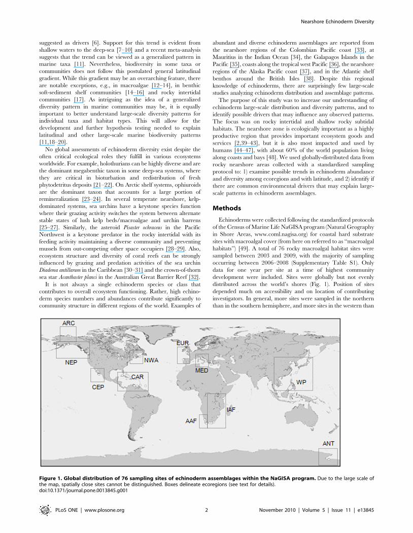
distributed across the world’s shores (Fig. 1). Position of sites

depended much on accessibility and on location of contributing

investigators. In general, more sites were sampled in the northern

than in the southern hemisphere, and more sites in the western than

Figure 1. Global distribution of 76 sampling sites of echinoderm assemblages within the NaGISA program. Due to the large scale ofthe map, spatially close sites cannot be distinguished. Boxes delineate ecoregions (see text for details).doi:10.1371/journal.pone.0013845.g001

Nearshore Echinoderm Diversity

PLoS ONE | www.plosone.org 2 November 2010 | Volume 5 | Issue 11 | e13845

in the eastern hemisphere. Several regions of the world’s coastline

were poorly sampled (e.g. Asia) or not at all sampled (e.g. Australia).

Sites were selected based on relatively pristine conditions and

remote from direct human influence as much as possible.

Sites were typically sampled at the high, mid and low intertidal

levels and at 1 m, 5 m, 10 m and occasionally 15 m subtidal depth

contours. Along each stratum, five replicate 0.0625 m2 quadrats

(from hereon referred to as 16x) were placed at randomly selected

(random number calculator) locations but with at least 1 m

distance between adjacent replicates. All epifaunal invertebrates

were removed from the quadrat area and echinoderms were

identified to the lowest taxonomic level possible (typically species

or genus). At several sites, echinoderms were enumerated using

1 m2 quadrats (from hereon referred to as 100x) either in addition

to or instead of the 16x quadrats (Supplementary Table S1). In the

100x quadrats, all visible echinoderms .2 cm were counted

without removal of the epifauna. Of the 76 macroalgal habitat

sites sampled, 12 were sampled only with 16x quadrats, 34 were

sampled only with 100x quadrats, and 30 sites were sampled with

both quadrat sizes (Supplementary Table S1). Data from the two

quadrat sizes were analyzed separately for all sites, resulting in four

assemblage types considered: 16x intertidal, 16x subtidal, 100x

intertidal, and 100x subtidal.

Local constraints prevented the sampling of all depth strata at

all sites. Abundance data were therefore averaged for intertidal

(high-low intertidal) and subtidal (1–15 m depths) regimes. Taxon

richness, a basic diversity measure, is particularly sensitive to

sampling effort with a higher likelihood to encounter more taxa

with increased sampling [50]. To appropriately address this

problem we used sample-based rarefaction to calculate the

expected number of taxa for five quadrats (ES5) at each site for

intertidal and subtidal assemblages [50–52]. Taxonomic distinct-

ness (D*), a diversity measure that is largely independent of

sampling effort and absolute abundances [53], was also obtained.

This index ranges from 0 to 100, allocating distances based on the

taxonomic level at which two taxa are related. Taxonomic levels

included in the analysis were species, genus, family, order, and

class, with equal weighting factors applied among all taxonomic

levels (Primer-E v6 software).

For large-scale comparisons of echinoderm abundance and

taxon richness (based on ES5 per site), sites were grouped into eco-

regions based on geography and prevailing oceanographic

conditions: Alaskan Arctic (ARC), north-east Pacific (NEP),

central-east Pacific (CEP), Mediterranean (MED), European

Atlantic (EUR), north-west Atlantic (NWA), Caribbean (CAR),

Indian Ocean Africa (IAF, warm Agulhas current influence),

Atlantic Ocean Africa (AAF, cold Benguela current influence),

Antarctic McMurdo Sound (ANT) (see Fig. 1 and Supplementary

Table S1). Regions with less than at least three sites for each

quadrat size/tidal regime combination were excluded (e.g.,

Western Pacific Asia, Atlantic South America). We caution that

all ecoregions likely were under-sampled to be a true represen-

tation of that region, but this grouping allowed for some

preliminary comparisons of larger-scale patterns above the local

variability. We therefore did not statistically compare abundance

and richness in ecoregions but we offer descriptive trends on

abundance and species composition and richness for ecoregions.

Relationships of abundance, ES5 and taxonomic distinctness with

latitude were analyzed using non-parametric Spearman Rank

Correlations (SPSS). To extract the effect of sampling effort (i.e.,

number of quadrats sampled per intertidal or subtial regime at

each site) on intertidal and subtidal abundance, in addition

quadrat numbers were regressed against abundance and the

residuals were used in correlations with latitude [54].

A set of 14 environmental drivers available for 54 sites within

ecoregions (Supplementary Table S1) were correlated with

biological site data pooled by ecoregion. We grouped environ-

mental variables into six ‘‘natural’’ and eight ‘‘anthropogenic’’

variables (Table 1). Natural environmental drivers included:

substrate type (SUB), macroalgal biomass (ALG), sea surface

temperature (SST), chlorophyll a (CHA), primary productivity

(PP), and salinity (SAL). Indices of anthropogenic variables of

inorganic pollution (INP), organic pollution (ORP), nutrient

contamination (NUTC), marine-derived pollution (MARP), acid-

ification (AC), invasive species incidence (INV), human coastal

population density (HUM), and shipping activity (SH) were taken

from 1 km resolution global models of human impacts on marine

ecosystems by Halpern et al. [55] (Table 1).

For the biological-environmental comparison we pooled

samples for the two tidal regimes (intertidal and subtidal) per site

and averaged both biological and environmental data for

ecoregions. Data for the quadrat sizes of 16x and 100x were

maintained separately. Only ecoregions that contained at least

three sites where biological and environmental data were available

were included in the analysis. We used ecoregions as the scale of

comparison because of the potential inaccuracy of satellite-derived

data from optical sea-surface properties (e.g., chlorophyll-a,

primary productivity) on small spatial scales [55]. Different

resolution of our biological data collected at a scale of 10’s of

meters (quadrats within the intertidal and subtidal regime of a

specific site) and environmental data extracted from global models

can be problematic. Although anthropogenic variables were

sampled at a 1 km resolution, the nearshore environment is

highly variable and can be under the influence of point sources. By

combining site data for ecoregions we concentrate on large-scale

variability, which exceeds the small-scale, local variability where

the above-mentioned uncertainties are most profound [56–57].

Biological communities over large spatial scales often do not

share any common species; hence, we used the taxonomic

dissimilarity coefficient Theta instead of the commonly-used

Bray-Curtis index for multivariate comparisons. Theta is based

on the presence/absence of species and the taxonomic relationship

(class to species used as taxonomic levels) of species within each

sample [58]. Theta dissimilarity matrices by ecoregions were

utilized to determine which environmental variables (also by

ecoregions) are most influential on echinoderm assemblages using

the BEST Bio-Env procedure within Primer-E. Only those sites

where both biological and environmental data were available were

included in the pooling of ecoregions and analyses (Supplementary

Table S1). Environmental variables were normalized to create a

common, dimensionless measurement scale and examined for

correlation prior to analysis using Spearman Rank correlations.

None of the variables were correlated at rho$0.95 and thus all

variables were maintained in the analyses. Analyses were

conducted including all environmental variables and, if variables

derived from satellite data (CHL and PP) were identified as

drivers, we repeated the analysis by excluding these variables to

assess any biases occurring from these data sources.

Results

Ecoregional patterns in echinoderm abundance anddiversity

A total of 86 echinoderm taxa were found across all sites, tidal

regimes and quadrat sizes; among these were 32 asteroids, 18

echinoids, 21 ophiuroids, and 15 holothuroids. In most ecoregions

variability among sites was high. Within intertidal assemblages

collected with 16x quadrats, highest abundances were found in the

Nearshore Echinoderm Diversity

PLoS ONE | www.plosone.org 3 November 2010 | Volume 5 | Issue 11 | e13845

Northeast Pacific (mean6se 14.465.9 ind 0.0625 m22) and the

Caribbean (3.963.7 ind 0.0625 m22) (Fig. 2a). In all other

regions, average abundance was less than 1 ind 0.0625 m22; no

echinoderms were found in the intertidal at only one site sampled

in the Mediterranean (data not shown). The abundant intertidal

assemblages in the Northeast Pacific were dominated by asteroids

and holothurians (Fig. 3a), represented nearly exclusively by

Leptasterias spp. and Cucumaria vegae, respectively. In the Caribbean,

mostly echinoids dominated by the two species, Echinometra viridis

and E. lucunter. Average abundances were also high in the

Northeast Pacific (5.162.5 ind 0.0625 m22) in the 16x subtidal

assemblages, but were not significantly different from those in the

Northwest Atlantic (2.861.7 ind 0.0625 m22) (Fig. 2b). Abun-

dances in both polar regions were less than 1 ind 0.0625 m22. The

abundant subtidal assemblages in the Northeast Pacific consisted

of a variety of species within four echinoderm classes (Fig. 3b):

asteroids (mostly Pycnopodia helianthoides, Evasterias troshelii, Henricia

leviuscula, Leptasterias spp., and Orthasterias koehleri), echinoids

(Strongylocentrotus droebachiensis), ophiuroids (mostly Amphipholis spp.

and Ophiopholis aculeata) and holothuroids (mostly Cucumaria vegae).

In the abundant 16x subtidal assemblages in the Northwest

Atlantic, asteroids were dominated by Asterias spp., echinoids by S.

droebachiensis, and ophiuroids by O. aculeata.

For intertidal assemblages sampled with the larger (100x)

quadrats, abundance was highest in the Caribbean (mean6se

5.261.3 ind m22) and on the African Indian Ocean coast

(2.161.0 ind m22), and was less than 1 ind m22 in all other

ecoregions (Fig. 2c). No echinoderms occurred at the two sites

collected in the West Pacific (data not shown). Echinoids

dominated in the Caribbean (Fig. 3c), specifically with Echinometra

viridis and E. lucunter and occasionally Diadema antillarum. All four

classes occurred in the African Indian Ocean but were dominated

by asteroids (mostly Patiriella exigua) and echinoids (especially

Parechinus angulosus and Echinometra mathaei). Abundances were not

significantly different among ecoregions in the subtidal assem-

blages from 100x quadrats, likely due to high variability among

sites within the Northwest Atlantic region, where abundance was

highest (11.6610.7 ind m22) (Fig. 2d). Assemblages there were

dominated by the echinoid Strongylocentrotus droebachiensis (Fig. 3d).

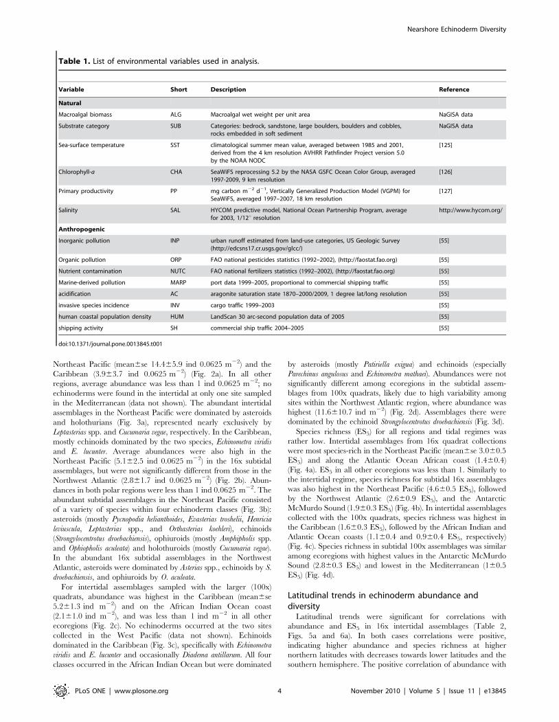
Species richness (ES5) for all regions and tidal regimes was

rather low. Intertidal assemblages from 16x quadrat collections

were most species-rich in the Northeast Pacific (mean6se 3.060.5

ES5) and along the Atlantic Ocean African coast (1.460.4)

(Fig. 4a). ES5 in all other ecoregions was less than 1. Similarly to

the intertidal regime, species richness for subtidal 16x assemblages

was also highest in the Northeast Pacific (4.660.5 ES5), followed

by the Northwest Atlantic (2.660.9 ES5), and the Antarctic

McMurdo Sound (1.960.3 ES5) (Fig. 4b). In intertidal assemblages

collected with the 100x quadrats, species richness was highest in

the Caribbean (1.660.3 ES5), followed by the African Indian and

Atlantic Ocean coasts (1.160.4 and 0.960.4 ES5, respectively)

(Fig. 4c). Species richness in subtidal 100x assemblages was similar

among ecoregions with highest values in the Antarctic McMurdo

Sound (2.860.3 ES5) and lowest in the Mediterranean (160.5

ES5) (Fig. 4d).

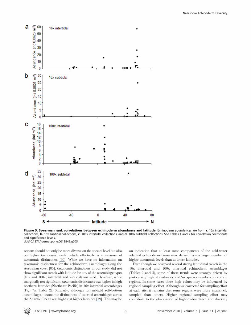
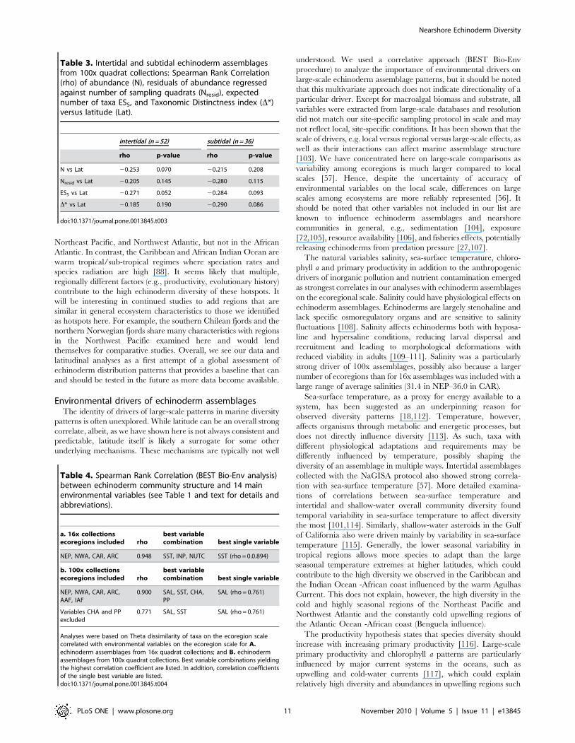
Latitudinal trends in echinoderm abundance anddiversity

Latitudinal trends were significant for correlations with

abundance and ES5 in 16x intertidal assemblages (Table 2,

Figs. 5a and 6a). In both cases correlations were positive,

indicating higher abundance and species richness at higher

northern latitudes with decreases towards lower latitudes and the

southern hemisphere. The positive correlation of abundance with

Table 1. List of environmental variables used in analysis.

Variable Short Description Reference

Natural

Macroalgal biomass ALG Macroalgal wet weight per unit area NaGISA data

Substrate category SUB Categories: bedrock, sandstone, large boulders, boulders and cobbles,rocks embedded in soft sediment

NaGISA data

Sea-surface temperature SST climatological summer mean value, averaged between 1985 and 2001,derived from the 4 km resolution AVHRR Pathfinder Project version 5.0by the NOAA NODC

[125]

Chlorophyll-a CHA SeaWiFS reprocessing 5.2 by the NASA GSFC Ocean Color Group, averaged1997-2009, 9 km resolution

[126]

Primary productivity PP mg carbon m22 d21, Vertically Generalized Production Model (VGPM) forSeaWiFS, averaged 1997–2007, 18 km resolution

[127]

Salinity SAL HYCOM predictive model, National Ocean Partnership Program, averagefor 2003, 1/12u resolution

http://www.hycom.org/

Anthropogenic

Inorganic pollution INP urban runoff estimated from land-use categories, US Geologic Survey(http://edcsns17.cr.usgs.gov/glcc/)

[55]

Organic pollution ORP FAO national pesticides statistics (1992–2002), (http://faostat.fao.org) [55]

Nutrient contamination NUTC FAO national fertilizers statistics (1992–2002), (http://faostat.fao.org) [55]

Marine-derived pollution MARP port data 1999–2005, proportional to commercial shipping traffic [55]

acidification AC aragonite saturation state 1870–2000/2009, 1 degree lat/long resolution [55]

invasive species incidence INV cargo traffic 1999–2003 [55]

human coastal population density HUM LandScan 30 arc-second population data of 2005 [55]

shipping activity SH commercial ship traffic 2004–2005 [55]

doi:10.1371/journal.pone.0013845.t001

Nearshore Echinoderm Diversity

PLoS ONE | www.plosone.org 4 November 2010 | Volume 5 | Issue 11 | e13845

latitude was slightly reduced in correlation strength and was

marginally not significant when abundance residuals were used

(i.e., corrected for sampling effort) (Table 2). These latitudinal

trends were likely driven mostly by the high values around 60u N,

i.e. the Northeast Pacific region (also see Figs. 2a and 4a). None of

the other correlations with latitude were significant (Table 2,

Figs. 5,6,7), although the correlation between taxonomic distinct-

ness and latitude for 16x intertidal assemblages was only

marginally non-significant (Table 2, Fig. 7a). Also the correlations

for both abundance and ES5 for 100x intertidal assemblages were

marginally non-significant (Table 3). Visual inspection of these

latter two correlation plots (Figs. 5c and 6c, respectively) indicated

that instead of a continuous gradient across both hemispheres,

there might be a peak at low latitudes (,10–11uN) with declines

towards higher latitudes at either side. Separate Spearman rank

correlations for abundances from 10–60uN and for 11uN–34uSwere both significant (rho = 20.550, p = 0.001 for 10–60uN;

rho = 0.484, p = 0.007 for 11uN–34uS), confirming highest abun-

dances at lower latitudes, i.e. in the Caribbean. Similarly, separate

Spearman rank correlations of ES5 with latitude for the same

latitudinal groups confirmed a significant decline in species

richness from low to high northern latitudes (10–60uN:

rho = 20.458, p = 0.005) while no significant decline into the

southern hemisphere was observed (11uN–34uS), but data

coverage in the southern hemisphere was low.

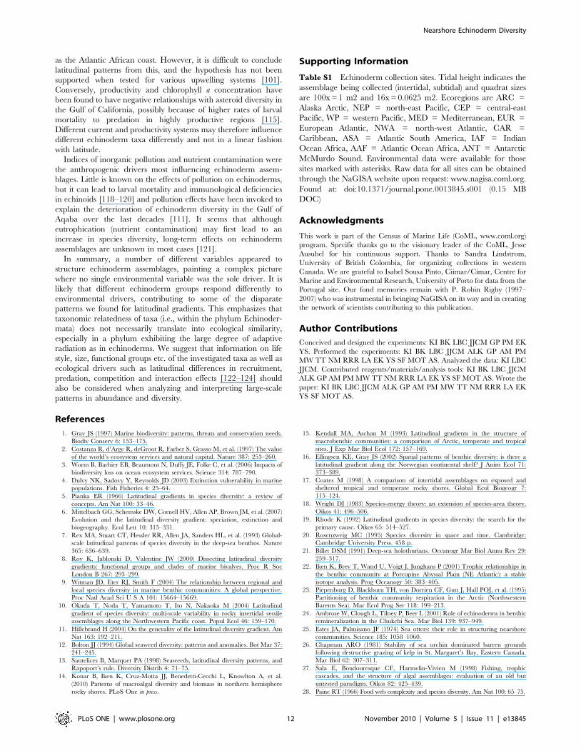
Correlation of echinoderm assemblages withenvironmental drivers

The highest correlation between the set of 14 environmental

variables and 16x assemblage data for the four ecoregions

Northeast Pacific, Northwest Atlantic, Caribbean and Alaskan

Arctic occurred with a combination of three variables (rho = 0.

948): sea-surface temperature, inorganic pollution and nutrient

contamination. The single variables sea-surface temperature and

inorganic pollution each by itself yielded a correlation of

rho = 0.894 (Table 4a). The combination of salinity, sea-surface

temperature, chlorophyll a and primary production correlated

strongly (rho = 0.900) with 100x assemblages for the six ecoregions

Northeast Pacific, Northwest Atlantic, Caribbean, Indian Ocean

African coast, Atlantic Ocean African coast and Alaskan Arctic.

Among these variables, salinity alone yielded the highest

coefficient with 100x ecoregional data (rho = 0.761, Table 4b).

When chlorophyll a and primary production as variables were

excluded from the 100x analysis because data derived from

spectral ocean properties may be associated with large errors,

especially in the nearshore system [55], overall correlation strength

was reduced (rho = 0.771) driven by salinity and sea-surface

temperature, with salinity remaining the most important variable

(rho = 0.761).

Discussion

Echinoderm diversity is typically higher in coastal regions than

deeper waters [34,59]; however, while echinoderms typically are a

conspicuous and abundant component within intertidal and

shallow subtidal habitats, they often are not overly diverse

compared to other phyla [37,60–62]. Similarly, species richness

in our collections from nearshore rocky macroalgal habitats was

low with typically only 1–5 species at those sites where

echinoderms were present. Several of our sites did not contain

Figure 2. Average echinoderm abundances in ecoregions. a. 16x intertidal collections, b. 16x subtidal collections, c. 100x intertidalcollections, d. 100x subtidal collections. Numbers below ecoregions specify the number of sites included in each region. See Fig. 1 and text forecoregions.doi:10.1371/journal.pone.0013845.g002

Nearshore Echinoderm Diversity

PLoS ONE | www.plosone.org 5 November 2010 | Volume 5 | Issue 11 | e13845

any echinoderms (18 of 76), irrespective of site location or

ecoregion. Despite low local diversity and abundance, echino-

derms often are ecologically important in intertidal and shallow

water systems, particularly as predators and grazers [63–65],

emphasizing the need to consider their large-scale distribution and

diversity patterns, such as latitudinal trends, and to identify

environmental drivers that may influence these assemblages.

Even though the low overall echinoderm species richness found

here is consistent with findings of other studies for intertidal and

shallow subtidal habitats [60–62], we emphasize that overall

species richness at any given site was certainly underestimated due

to the sampling scheme used. The use of the standardized

NaGISA sampling protocol [49] is useful for comparison of

sample-based diversity among sites [51], also referred to as point

diversity [66–67] or species density [51], but is not a reliable tool

to comprehensively assess local (alpha) diversity within a

community [68–69]. While it is not always obvious how a

community would be defined for the assessment of alpha diversity

[68], the 5–15 replicate quadrats per tidal range as collected here

are not likely to inventory the entire community. Hence, data

collected with the NaGISA protocol or similar standardized

sampling designs will only represent a subset of the species

occurring in a certain community, i.e., a subset of alpha diversity.

The benefit of using this species density as a measure in large-scale

comparisons is that there is no ambiguity of defining the scale of

community as it exists for alpha diversity. Other benefits lie in the

comparability of a standardized sampling effort and the practical-

ity of how many replicate samples can feasibly be processed if

large-scale coverage is the goal. The efficiency of quadrat sampling

is dependent on the size and distribution patterns of the target

organisms and may not be as effective in assessing patterns of

highly patchily distributed taxa such as echinoderms [70–71]. The

100x quadrats (only organisms .2 cm collected) targeted larger-

sized echinoderms, mostly adult asteroids and echinoids (see Fig. 3c

and d) that typically are patchily distributed. In comparison, many

small-sized ophiuroids and holothurians, and juvenile asteroids

and echinoids were included in the collections from the 16x

quadrats, which often occur in large densities. Therefore, the

observed differences between assemblages with respect to different

quadrat sizes are not surprising as the spatial patterns of diversity

can be influenced by the scale at which those observations are

made [9–10,72–73]. We propose that visual assessments of

echinoderm richness should rather be done with belt transects

than 161 m quadrats because of the typically large size and

patchy distribution of most echinoderm species.

Large-scale trends in echinoderm assemblagesAbundance and species richness (ES5) in assemblages from the

100x intertidal collections followed the suggested generalized

latitudinal gradient pattern [11], with highest values at low latitudes

(Caribbean) and clines in both hemispheres towards higher latitudes.

In the Caribbean, these assemblages consisted mainly of echinoids

(see Fig. 3c). Similar peaks in sea urchin abundance and diversity at

low latitudes have been found previously in regional-scale investiga-

Figure 3. Relative abundances of echinoderm classes in ecoregions. a. 16x intertidal collections, b. 16x subtidal collections, c. 100x intertidalcollections, d. 100x subtidal collections. Numbers below ecoregions specify the number of sites included in each region. See Fig 1 and text forecoregions.doi:10.1371/journal.pone.0013845.g003

Nearshore Echinoderm Diversity

PLoS ONE | www.plosone.org 6 November 2010 | Volume 5 | Issue 11 | e13845

tions in the Mediterranean [74]. The causes for this pattern are

uncertain but may be related to a prevalence of thermophilic species

in sea urchins [75], latitudinal differences in recruitment success

[76–77] and salinity tolerance [78], competitive and predatory

interactions [79–80], relief from predation due to overfishing [27], as

well as high adaptability of sea urchins to environmental stress

[81–82]. The latter is likely relaxed for subtidal communities because

of generally more buffered physical environmental conditions in the

subtidal [83], and may contribute to the non-significant abundance

and diversity patterns in the 100x subtidal assemblages.

In contrast to the 100x intertidal assemblages, the 16x intertidal

assemblages showed a gradient of highest abundance and richness

at high northern latitudes with declines towards lower latitudes.

These declines continued into the southern hemisphere, although

sample coverage there was low and our patterns in the southern

hemisphere have to be considered with care within a global

context. Latitudinal trends observed here therefore are mainly

driven by, and are most relevant for, the more intensively sampled

northern hemisphere. This latitudinal decline in 16x intertidal

echinoderm assemblage abundance and richness was mostly

driven by high values in the Northeast Pacific, a highly productive

and diverse ecoregion [62,84]. Correlation strength of this

latitudinal cline in 16x intertidal assemblages was moderate

(0.32–0.46 for abundance and 0.42 for ES5, Table 2) but was

comparable or even stronger than correlation strengths found in

other studies observing marine latitudinal gradients (e.g., 0.13–

0.39) [9]. Most notably, the latitudinal pattern of highest diversity

in high northern latitudes (as observed for 16x intertidal

assemblages) is not consistent with the postulated pattern of low

latitudinal diversity peaks [11].

The lack of other global or truly large-scale diversity studies for

echinoderms limits our comparisons to regional studies. For

example, echinoderm diversity along the eastern Australian coast

down to Tasmania decreased with increasing latitude [85], similar

to what we observed for 100x intertidal echinoderms. In Australia

this pattern was argued to be related mostly to the geological history

of the continent, which favored continued immigration of new

species from the tropics in Australia’s north but led to progressive

exclusion of cold-water species and survival of only few adaptive

genera in the high-latitude south [85,86]. Immigration in addition

to vicariance has often been presented to explain higher diversity in

tropical compared to temperate regions [87–89]. One would expect

that as a result of such evolutionary patterns, tropical or low latitude

Figure 4. Expected number of species (ES5) in ecoregions. a. 16x intertidal collections, b. 16x subtidal collections, c. 100x intertidalcollections, d. 100x subtidal collections. Numbers below ecoregions specify the number of sites included in each region. See Fig. 1 and text forecoregions.doi:10.1371/journal.pone.0013845.g004

Table 2. Intertidal and subtidal echinoderm assemblagesfrom 16x quadrat collections: Spearman Rank Correlation (rho)of abundance (N), residuals of abundance regressed againstnumber of sampling quadrats (Nresid), expected number oftaxa ES5, and Taxonomic Distinctness index (D*) versuslatitude (Lat).

intertidal (n = 26) subtidal (n = 31)

rho p-value rho p-value

N vs Lat 0.463 0.017 20.236 0.166

Nresid vs Lat 0.322 0.051 20.317 0.059

ES5 vs Lat 0.422 0.032 20.059 0.734

D* vs Lat 0.377 0.063 20.306 0.094

Bold print indicates significant correlations at a#0.05.doi:10.1371/journal.pone.0013845.t002

Nearshore Echinoderm Diversity

PLoS ONE | www.plosone.org 7 November 2010 | Volume 5 | Issue 11 | e13845

regions should not only be more diverse on the species level but also

on higher taxonomic levels, which effectively is a measure of

taxonomic distinctness [90]. While we have no information on

taxonomic distinctness for the echinoderm assemblages along the

Australian coast [85], taxonomic distinctness in our study did not

show significant trends with latitude for any of the assemblage types

(16x and 100x, intertidal and subtidal) analyzed. However, while

marginally not significant, taxonomic distinctness was higher in high

northern latitudes (Northeast Pacific) in 16x intertidal assemblages

(Fig. 7a, Table 2). Similarly, although for subtidal soft-bottom

assemblages, taxonomic distinctness of asteroid assemblages across

the Atlantic Ocean was highest at higher latitudes [59]. This may be

an indication that at least some components of the cold-water

adapted echinoderm fauna may derive from a larger number of

higher taxonomic levels than at lower latitudes.

Even though we observed several strong latitudinal trends in the

16x intertidal and 100x intertidal echinoderm assemblages

(Tables 2 and 3), some of these trends were strongly driven by

particularly high abundances and/or species numbers in certain

regions. In some cases these high values may be influenced by

regional sampling effort. Although we corrected for sampling effort

at each site, it remains that some regions were more intensively

sampled than others. Higher regional sampling effort may

contribute to the observation of higher abundance and diversity

Figure 5. Spearman rank correlations between echinoderm abundance and latitude. Echinoderm abundances are from a. 16x intertidalcollections, b. 16x subtidal collections, c. 100x intertidal collections, and d. 100x subtidal collections. See Tables 1 and 2 for correlation coefficientsand significance levels.doi:10.1371/journal.pone.0013845.g005

Nearshore Echinoderm Diversity

PLoS ONE | www.plosone.org 8 November 2010 | Volume 5 | Issue 11 | e13845

measures. For example, high sampling effort in the Northeast

Pacific 16x intertidal coincided with high abundances and species

richness. This is not a general pattern, however, as, for example,

the large number of sites sampled for the 100x intertidal in the

Northeast Pacific resulted in low abundance and species richness

for that assemblage type (Figs. 2 and 4, respectively). Similarly,

even though for the 16x subtidal assemblages the highest number

of sites (11 sites) was sampled in the Arctic, abundances and species

richness remained very low. Still, differences in regional sampling

effort are likely to influence any latitudinal or other large-scale

comparisons. Sufficient replication per latitude or latitudinal

ranges and increased coverage of especially southern hemisphere

coastlines will be needed for the evaluation of reliable global

trends. Even though our data coverage is the most comprehensive

currently available for echinoderms from nearshore rocky

macroalgal habitats, we still lack sufficient coverage along many

coastlines and latitudinal ranges.

It also is likely that overall latitudinal trends are interspersed

with regional hotspots that disrupt, or go against, the main trend.

Several ecoregions may be identified as hotspots for nearshore

echinoderms in rocky habitats based on their overall high

echinoderm abundance and species richness, e.g., in the

Caribbean, the Northeast Pacific, the Northwest Atlantic, the

Atlantic and Indian African coasts, and the Antarctic McMurdo

Sound. It is possible that regional and local conditions act on top

of latitudinal location and influence patterns in echinoderm

Figure 6. Spearman rank correlations between echinoderm species richness (based on estimated number of species ES5) andlatitude. Echinoderm abundances are from a. 16x intertidal collections, b. 16x subtidal collections, c. 100x intertidal collections, and d. 100x subtidalcollections. See Tables 1 and 2 for correlation coefficients and significance levels.doi:10.1371/journal.pone.0013845.g006

Nearshore Echinoderm Diversity

PLoS ONE | www.plosone.org 9 November 2010 | Volume 5 | Issue 11 | e13845

assemblages. For example, Price et al. [59] found that shallow-

water asteroid assemblages across the Atlantic Ocean were more

distinct by geographic region and the level of isolation among

regions than by latitude. In the Antarctic, echinoderm assemblages

were more influenced by a combination of local and regional

processes such as oceanographic conditions and iceberg scour

intensity than by latitude [91]. We also observed relatively high

diversity in subtidal echinoderm assemblages in the Antarctic, a

region that is known to have high diversity for many taxa based on

the long evolutionary isolation of the Southern Ocean, and high

nutrient levels leading to high primary productivity [92–95]. In

contrast, the low abundance and species richness we found in the

Arctic region is consistent with other observations of a sharp

decline in diversity in the Arctic compared to northern high

latitudes, due to the severe ice impact and low food abundance in

the Arctic [61,96–100]. Among the ecoregions that may be

hotspots, the Northeast Pacific, Northwest Atlantic, African

Atlantic and Antarctic all are highly productive regions

[40,84,101] providing rich food sources for nearshore echino-

derms in rocky habitats [102]. Typically, this should also be

reflected in high abundances, which we found in some echinoderm

assemblages (esp. 16x intertidal and subtidal, Fig. 2) in the

Figure 7. Spearman rank correlations between echinoderm taxonomic distinctness and latitude. Echinoderm abundances are from a.16x intertidal collections, b. 16x subtidal collections, c. 100x intertidal collections, and d. 100x subtidal collections. See Tables 1 and 2 for correlationcoefficients and significance levels.doi:10.1371/journal.pone.0013845.g007

Nearshore Echinoderm Diversity

PLoS ONE | www.plosone.org 10 November 2010 | Volume 5 | Issue 11 | e13845

Northeast Pacific, and Northwest Atlantic, but not in the African

Atlantic. In contrast, the Caribbean and African Indian Ocean are

warm tropical/sub-tropical regimes where speciation rates and

species radiation are high [88]. It seems likely that multiple,

regionally different factors (e.g., productivity, evolutionary history)

contribute to the high echinoderm diversity of these hotspots. It

will be interesting in continued studies to add regions that are

similar in general ecosystem characteristics to those we identified

as hotspots here. For example, the southern Chilean fjords and the

northern Norwegian fjords share many characteristics with regions

in the Northwest Pacific examined here and would lend

themselves for comparative studies. Overall, we see our data and

latitudinal analyses as a first attempt of a global assessment of

echinoderm distribution patterns that provides a baseline that can

and should be tested in the future as more data become available.

Environmental drivers of echinoderm assemblagesThe identity of drivers of large-scale patterns in marine diversity

patterns is often unexplored. While latitude can be an overall strong

correlate, albeit, as we have shown here is not always consistent and

predictable, latitude itself is likely a surrogate for some other

underlying mechanisms. These mechanisms are typically not well

understood. We used a correlative approach (BEST Bio-Env

procedure) to analyze the importance of environmental drivers on

large-scale echinoderm assemblage patterns, but it should be noted

that this multivariate approach does not indicate directionality of a

particular driver. Except for macroalgal biomass and substrate, all

variables were extracted from large-scale databases and resolution

did not match our site-specific sampling protocol in scale and may

not reflect local, site-specific conditions. It has been shown that the

scale of drivers, e.g. local versus regional versus large-scale effects, as

well as their interactions can affect marine assemblage structure

[103]. We have concentrated here on large-scale comparisons as

variability among ecoregions is much larger compared to local

scales [57]. Hence, despite the uncertainty of accuracy of

environmental variables on the local scale, differences on large

scales among ecosystems are more reliably represented [56]. It

should be noted that other variables not included in our list are

known to influence echinoderm assemblages and nearshore

communities in general, e.g., sedimentation [104], exposure

[72,105], resource availability [106], and fisheries effects, potentially

releasing echinoderms from predation pressure [27,107].

The natural variables salinity, sea-surface temperature, chloro-

phyll a and primary productivity in addition to the anthropogenic

drivers of inorganic pollution and nutrient contamination emerged

as strongest correlates in our analyses with echinoderm assemblages

on the ecoregional scale. Salinity could have physiological effects on

echinoderm assemblages. Echinoderms are largely stenohaline and

lack specific osmoregulatory organs and are sensitive to salinity

fluctuations [108]. Salinity affects echinoderms both with hyposa-

line and hypersaline conditions, reducing larval dispersal and

recruitment and leading to morphological deformations with

reduced viability in adults [109–111]. Salinity was a particularly

strong driver of 100x assemblages, possibly also because a larger

number of ecoregions than for 16x assemblages was included with a

large range of average salinities (31.4 in NEP–36.0 in CAR).

Sea-surface temperature, as a proxy for energy available to a

system, has been suggested as an underpinning reason for

observed diversity patterns [18,112]. Temperature, however,

affects organisms through metabolic and energetic processes, but

does not directly influence diversity [113]. As such, taxa with

different physiological adaptations and requirements may be

differently influenced by temperature, possibly shaping the

diversity of an assemblage in multiple ways. Intertidal assemblages

collected with the NaGISA protocol also showed strong correla-

tion with sea-surface temperature [57]. More detailed examina-

tions of correlations between sea-surface temperature and

intertidal and shallow-water overall community diversity found

temporal variability in sea-surface temperature to affect diversity

the most [101,114]. Similarly, shallow-water asteroids in the Gulf

of California also were driven mainly by variability in sea-surface

temperature [115]. Generally, the lower seasonal variability in

tropical regions allows more species to adapt than the large

seasonal temperature extremes at higher latitudes, which could

contribute to the high diversity we observed in the Caribbean and

the Indian Ocean -African coast influenced by the warm Agulhas

Current. This does not explain, however, the high diversity in the

cold and highly seasonal regions of the Northeast Pacific and

Northwest Atlantic and the constantly cold upwelling regions of

the Atlantic Ocean -African coast (Benguela influence).

The productivity hypothesis states that species diversity should

increase with increasing primary productivity [116]. Large-scale

primary productivity and chlorophyll a patterns are particularly

influenced by major current systems in the oceans, such as

upwelling and cold-water currents [117], which could explain

relatively high diversity and abundances in upwelling regions such

Table 3. Intertidal and subtidal echinoderm assemblagesfrom 100x quadrat collections: Spearman Rank Correlation(rho) of abundance (N), residuals of abundance regressedagainst number of sampling quadrats (Nresid), expectednumber of taxa ES5, and Taxonomic Distinctness index (D*)versus latitude (Lat).

intertidal (n = 52) subtidal (n = 36)

rho p-value rho p-value

N vs Lat 20.253 0.070 20.215 0.208

Nresid vs Lat 20.205 0.145 20.280 0.115

ES5 vs Lat 20.271 0.052 20.284 0.093

D* vs Lat 20.185 0.190 20.290 0.086

doi:10.1371/journal.pone.0013845.t003

Table 4. Spearman Rank Correlation (BEST Bio-Env analysis)between echinoderm community structure and 14 mainenvironmental variables (see Table 1 and text for details andabbreviations).

a. 16x collectionsecoregions included rho

best variablecombination best single variable

NEP, NWA, CAR, ARC 0.948 SST, INP, NUTC SST (rho = 0.0.894)

b. 100x collectionsecoregions included rho

best variablecombination best single variable

NEP, NWA, CAR, ARC,AAF, IAF

0.900 SAL, SST, CHA,PP

SAL (rho = 0.761)

Variables CHA and PPexcluded

0.771 SAL, SST SAL (rho = 0.761)

Analyses were based on Theta dissimilarity of taxa on the ecoregion scalecorrelated with environmental variables on the ecoregion scale for A.echinoderm assemblages from 16x quadrat collections; and B. echinodermassemblages from 100x quadrat collections. Best variable combinations yieldingthe highest correlation coefficient are listed. In addition, correlation coefficientsof the single best variable are listed.doi:10.1371/journal.pone.0013845.t004

Nearshore Echinoderm Diversity

PLoS ONE | www.plosone.org 11 November 2010 | Volume 5 | Issue 11 | e13845

as the Atlantic African coast. However, it is difficult to conclude

latitudinal patterns from this, and the hypothesis has not been

supported when tested for various upwelling systems [101].

Conversely, productivity and chlorophyll a concentration have

been found to have negative relationships with asteroid diversity in

the Gulf of California, possibly because of higher rates of larval

mortality to predation in highly productive regions [115].

Different current and productivity systems may therefore influence

different echinoderm taxa differently and not in a linear fashion

with latitude.

Indices of inorganic pollution and nutrient contamination were

the anthropogenic drivers most influencing echinoderm assem-

blages. Little is known on the effects of pollution on echinoderms,

but it can lead to larval mortality and immunological deficiencies

in echinoids [118–120] and pollution effects have been invoked to

explain the deterioration of echinoderm diversity in the Gulf of

Aqaba over the last decades [111]. It seems that although

eutrophication (nutrient contamination) may first lead to an

increase in species diversity, long-term effects on echinoderm

assemblages are unknown in most cases [121].

In summary, a number of different variables appeared to

structure echinoderm assemblages, painting a complex picture

where no single environmental variable was the sole driver. It is

likely that different echinoderm groups respond differently to

environmental drivers, contributing to some of the disparate

patterns we found for latitudinal gradients. This emphasizes that

taxonomic relatedness of taxa (i.e., within the phylum Echinoder-

mata) does not necessarily translate into ecological similarity,

especially in a phylum exhibiting the large degree of adaptive

radiation as in echinoderms. We suggest that information on life

style, size, functional groups etc. of the investigated taxa as well as

ecological drivers such as latitudinal differences in recruitment,

predation, competition and interaction effects [122–124] should

also be considered when analyzing and interpreting large-scale

patterns in abundance and diversity.

Supporting Information

Table S1 Echinoderm collection sites. Tidal height indicates the

assemblage being collected (intertidal, subtidal) and quadrat sizes

are 100x = 1 m2 and 16x = 0.0625 m2. Ecoregions are ARC =

Alaska Arctic, NEP = north-east Pacific, CEP = central-east

Pacific, WP = western Pacific, MED = Mediterranean, EUR =

European Atlantic, NWA = north-west Atlantic, CAR =

Caribbean, ASA = Atlantic South America, IAF = Indian

Ocean Africa, AAF = Atlantic Ocean Africa, ANT = Antarctic

McMurdo Sound. Environmental data were available for those

sites marked with asterisks. Raw data for all sites can be obtained

through the NaGISA website upon request: www.nagisa.coml.org.

Found at: doi:10.1371/journal.pone.0013845.s001 (0.15 MB

DOC)

Acknowledgments

This work is part of the Census of Marine Life (CoML, www.coml.org)

program. Specific thanks go to the visionary leader of the CoML, Jesse

Ausubel for his continuous support. Thanks to Sandra Lindstrom,

University of British Colombia, for organizing collections in western

Canada. We are grateful to Isabel Sousa Pinto, Ciimar/Cimar, Centre for

Marine and Environmental Research, University of Porto for data from the

Portugal site. Our fond memories remain with P. Robin Rigby (1997–

2007) who was instrumental in bringing NaGISA on its way and in creating

the network of scientists contributing to this publication.

Author Contributions

Conceived and designed the experiments: KI BK LBC JJCM GP PM EK

YS. Performed the experiments: KI BK LBC JJCM ALK GP AM PM

MW TT NM RRR LA EK YS SF MOT AS. Analyzed the data: KI LBC

JJCM. Contributed reagents/materials/analysis tools: KI BK LBC JJCM

ALK GP AM PM MW TT NM RRR LA EK YS SF MOT AS. Wrote the

paper: KI BK LBC JJCM ALK GP AM PM MW TT NM RRR LA EK

YS SF MOT AS.

References

1. Gray JS (1997) Marine biodiversity: patterns, threats and conservation needs.

Biodiv Conserv 6: 153–175.

2. Costanza R, d’Arge R, deGroot R, Farber S, Grasso M, et al. (1997) The value

of the world’s ecosystem services and natural capital. Nature 387: 253–260.

3. Worm B, Barbier EB, Beaumont N, Duffy JE, Folke C, et al. (2006) Impacts of

biodiversity loss on ocean ecosystem services. Science 314: 787–790.

4. Dulvy NK, Sadovy Y, Reynolds JD (2003) Extinction vulnerability in marine

populations. Fish Fisheries 4: 25–64.

5. Pianka ER (1966) Latitudinal gradients in species diversity: a review of

concepts. Am Nat 100: 33–46.

6. Mittelbach GG, Schemske DW, Cornell HV, Allen AP, Brown JM, et al. (2007)

Evolution and the latitudinal diversity gradient: speciation, extinction and

biogeography. Ecol Lett 10: 315–331.

7. Rex MA, Stuart CT, Hessler RR, Allen JA, Sanders HL, et al. (1993) Global-

scale latitudinal patterns of species diversity in the deep-sea benthos. Nature

365: 636–639.

8. Roy K, Jablonski D, Valentine JW (2000) Dissecting latitudinal diversity

gradients: functional groups and clades of marine bivalves. Proc R Soc

London B 267: 293–299.

9. Witman JD, Eter RJ, Smith F (2004) The relationship between regional and

local species diversity in marine benthic communities: A global perspective.

Proc Natl Acad Sci U S A 101: 15664–15669.

10. Okuda T, Noda T, Yamamoto T, Ito N, Nakaoka M (2004) Latitudinal

gradient of species diversity: multi-scale variability in rocky intertidal sessile

assemblages along the Northwestern Pacific coast. Popul Ecol 46: 159–170.

11. Hillebrand H (2004) On the generality of the latitudinal diversity gradient. Am

Nat 163: 192–211.

12. Bolton JJ (1994) Global seaweed diversity: patterns and anomalies. Bot Mar 37:

241–245.

13. Santelices B, Marquet PA (1998) Seaweeds, latitudinal diversity patterns, and

Rapoport’s rule. Diversity Distrib 4: 71–75.

14. Konar B, Iken K, Cruz-Motta JJ, Benedetti-Cecchi L, Knowlton A, et al.

(2010) Patterns of macroalgal diversity and biomass in northern hemisphere

rocky shores. PLoS One in press.

15. Kendall MA, Aschan M (1993) Latitudinal gradients in the structure of

macrobenthic communities: a comparison of Arctic, temperate and tropical

sites. J Exp Mar Biol Ecol 172: 157–169.

16. Ellingsen KE, Gray JS (2002) Spatial patterns of benthic diversity: is there a

latitudinal gradient along the Norwegian continental shelf? J Anim Ecol 71:

373–389.

17. Coates M (1998) A comparison of intertidal assemblages on exposed and

sheltered tropical and temperate rocky shores. Global Ecol Biogeogr 7:

115–124.

18. Wright DJ (1983) Species-energy theory: an extension of species-area theory.

Oikos 41: 496–506.

19. Rhode K (1992) Latitudinal gradients in species diversity: the search for the

primary cause. Oikos 65: 514–527.

20. Rosenzweig MC (1995) Species diversity in space and time. Cambridge:

Cambridge University Press. 458 p.

21. Billet DSM (1991) Deep-sea holothurians. Oceanogr Mar Biol Annu Rev 29:

259–317.

22. Iken K, Brey T, Wand U, Voigt J, Junghans P (2001) Trophic relationships in

the benthic community at Porcupine Abyssal Plain (NE Atlantic): a stable

isotope analysis. Prog Oceanogr 50: 383–405.

23. Piepenburg D, Blackburn TH, von Dorrien CF, Gutt J, Hall POJ, et al. (1995)

Partitioning of benthic community respiration in the Arctic (Northwestern

Barents Sea). Mar Ecol Prog Ser 118: 199–213.

24. Ambrose W, Clough L, Tilney P, Beer L (2001) Role of echinoderms in benthic

remineralization in the Chukchi Sea. Mar Biol 139: 937–949.

25. Estes JA, Palmisano JF (1974) Sea otters: their role in structuring nearshore

communities. Science 185: 1058–1060.

26. Chapman ARO (1981) Stability of sea urchin dominated barren grounds

following destructive grazing of kelp in St. Margaret’s Bay, Eastern Canada.

Mar Biol 62: 307–311.

27. Sala E, Boudouresque CF, Harmelin-Vivien M (1998) Fishing, trophic

cascades, and the structure of algal assemblages: evaluation of an old but

untested paradigm. Oikos 82: 425–439.

28. Paine RT (1966) Food web complexity and species diversity. Am Nat 100: 65–75.

Nearshore Echinoderm Diversity

PLoS ONE | www.plosone.org 12 November 2010 | Volume 5 | Issue 11 | e13845

29. McClintock JB, Robnett TJ (1986) Size selective predation by the asteroid

Pisaster ochraceus on the bivalve Mytilus californianus: a cost benefit analysis. Mar

Ecol 7: 321–332.

30. Sammarco PW (1980) Diadema and its relationship to coral spat mortality:

grazing, competition, and biological disturbance. J Exp Mar Biol Ecol 45:

245–272.

31. Edmunds PJ, Carpenter RC (2001) Recovery of Diadema antillarum reduces

macroalgal cover and increases abundance of juvenile corals on a Caribbean

reef. Proc Natl Acad Sci U S A 98: 5067–5071.

32. Porter JW (1972) Predation by Acanthaster and its effect on coral species

diversity. Am Nat 106: 487–492.

33. Neira R, Cantera JR (2005) Taxonomic composition and distribution of the

echinoderm associations in the littoral ecosystems from the Colombian Pacific.

Rev Biol Trop 53: 195–206.

34. Rowe FEW, Richmond MD (2004) A preliminary account of the shallow-water

echinoderms of Rodrigues, Mauritius, western Indian Ocean. J Nat Hist 38:

3273–3314.

35. Hickman CP (2009) Evolutionary responses of marine invertebrates to insular

isolation in Galapagos. Galapagos Res 66: 32–42.

36. Pearse JS (2009) Shallow-water asteroids, echinoids, and holothuroids at 6 sites

across the tropical west Pacific, 1988-1989. Galaxea, J Coral Reef Stud 11: 1–9.

37. Chenelot HA, Iken K, Konar B, Edwards M (2007) Spatial and temporal

distribution of echinoderms in rocky nearshore areas of Alaska. In: Rigby PR,

Shirayama Y, editors. Selected papers of the NaGISA world congress 2006.

Publications of the Seto Marine Biological Laboratory, Special Publication

Series 8: 11–28.

38. Ellis JR, Rogers SI (2000) The distribution, relative abundance and diversity of

echinoderms in the eastern English Channel, Bristol Channel, and Irish Sea.

J Mar Biol Ass U K 80: 127–138.

39. Leigh EG, Jr., Paine RT, Quinn JF, Suchanek TH (1987) Wave energy and

intertidal productivity. Proc Natl Acad Sci U S A 84: 1314–1318.

40. Bustamante RH, Branch GM, Eekhout S, Robertson B, Zoutendyk P, et al.

(1995) Gradients of intertidal primary productivity around the coast of South

Africa and their relationships with consumer biomass. Oecologia 102: 189–201.

41. Menge BA, Daley BA, Wheeler PA, Dahlhoff E, Sanford E, et al. (1997)

Benthic-pelagic links and rocky intertidal communities: bottom-up effects on

top-down control? Proc Natl Acad Sci USA 26: 14530–14535.

42. Beck MW, Heck KL, Jr., Able KW, Childers DL, Eggleston DB, et al. (2003)

The role of nearshore ecosystems as fish and shellfish nurseries. Issues Ecol 11:

1–12.

43. Ronnback P, Kautsky N, Pihl L, Troell M, Soderqvist T, et al. (2007)

Ecosystem goods and services from Swedish coastal habitats: identification,

valuation, and implications of ecosystem shifts. Ambio 36: 534–544.

44. Beauchamp KA, Gowing MM (1982) A quantitative assessment of human

trampling effects on a rocky intertidal community. Mar Environ Res 7:

279–293.

45. Adessi L (1994) Human disturbance and long-term changes on a rocky

intertidal community. Ecol Appl 4: 786–797.

46. Thompson RC, Crowe TP, Hawkins SJ (2002) Rocky intertidal communities:

past environmental changes, present status and predictions for the next 25

years. Environ Conserv 29: 168–191.

47. Airoldi L, Beck MW (2007) Loss, status and trends for coastal marine habitats

of Europe. Oceanogr Mar Biol Annu Rev 45: 345–405.

48. Lindeboom H (2002) The coastal zone: an ecosystem under pressure. In:

Field JG, Hampel G, Summerhayes C, eds. Oceans 2020: science, trends and

the challenge of sustainability. Washington, DC: Island Press. pp 49–84.

49. Rigby PR, Iken K, Shirayama Y (2007) Sampling Diversity in Coastal

Communities. NaGISA Protocols for Seagrass and Macroalgal Habitats. Kyoto

University Press. 145 p.

50. Gotelli NJ, Colwell RK (2001) Quantifying biodiversity: procedures and pitfalls

in the measurement and comparison of species richness. Ecol Lett 4: 379–391.

51. Smith EP, Stewart PM, Cairna J (1985) Similarities between rarefactionmethods. Hydrobiol 120: 167–170.

52. Chiarucci A, Bacaro G, Rocchini D, Fattorini L (2008) Discovering and

rediscovering the sample-based rarefaction formula in the ecological literature.

Commun Ecol 9: 121–123.

53. Clarke KR, Warwick RM (2001) Change in marine communities. An approach

to statistical analysis and interpretation. 2nd edition. PRIMER-E, Plymouth,

UK, 172 p.

54. Sokal RR, Rohlf JF (1995) Biometry: the principles and practice of statistics in

biological research (3rd edition). WH Freeman and Company: New York,

USA. 887 p.

55. Halpern BS, Walbridge S, Selkoe KA, Kappel CV, Micheli F, et al. (2008) A

global map of human impact on marine ecosystems. Science 319: 948–952.

56. Benedetti-Cecchi L, Iken K, Konar B, Cruz-Motta JJ, Knowlton K, et al.

(2010) Spatial relationships between polychaete assemblages and environmen-

tal variables over broad geographical scale. PLoS One 5: e12946. doi:10.1371/

journal.pone.0012946.

57. Cruz-Motta JJ, Miloslavich P, Palomo G, Iken K, Konar B, et al. (2010)

Patterns of spatial variation of assemblages associated with intertidal rocky

shores: a global perspective. PLoS One in press.

58. Clarke KR, Somerfield PJ, Chapman MG (2006) On resemblance measures for

ecological studies, including taxonomic dissimilarities and a zero-adjusted

Bray–Curtis coefficient for denuded assemblages. J Exp Mar Biol Ecol 330:55–80.

59. Price ARG, Keeling MJ, O’Callaghan CJ (1999) Ocean-scale patterns of

‘‘biodiversity’’ of Atlantic asteroids determined from taxonomic distinctness

and other measures. Biol J Linn Soc 66: 187–203.

60. Benkendorff K (2005) Intertidal molluscan and echinoderm diversity at

Althorpe Island and Innes National Park, South Australia. Trans R Soc South

Australia 129: 145–157.

61. Kuklinski P, Barnes DKA, Taylor PD (2006) Latitudinal patterns of diversity

and abundance in North Atlantic intertidal boulder-fields. Mar Biol 149:

1577–1583.

62. Konar B, Iken K, Edwards M (2009) Depth-stratified community zonation

patterns on Gulf of Alaska rocky shores. Mar Ecol 30: 63–73.

63. Paine RT (1974) Intertidal community structure. Oecologia 15: 93–120.

64. Sousa WP, Schroeter SC, Gaines SD (1981) Latitudinal variation in intertidal

algal community structure: the influence of grazing and vegetative propagation.

Oecologia 48: 297–307.

65. Benedetti-Cecchi L, Cinelli F (1995) Habitat heterogeneity, sea urchin grazing

and the distribution of algae in littoral rock pools on the west coast of Italy

(western Mediterranean). Mar Ecol Prog Ser 126: 203–212.

66. Willig MR, Kaufman DM, Stevens RD (2003) Latiudinal Gradients of

Biodiversity: Patterns, Process, Scale, and Synthesis. Annu Rev Ecol Evol Syst

34: 273–309.

67. Magurran AE (2009) Measuring Biological Diversity. Blackwell Publishing:

Oxford, UK. 256 p.

68. Underwood AJ (1989) What is a community? In: Raup DM, Jablonski D, eds.Patterns and processes in the history of life. Springer: Berlin. pp 351–367.

69. Gray JS (2000) The measurement of marine species diversity, with an

application to the benthic fauna of the Norwegian continental shelf. J Exp MarBiol Ecol 250: 23–49.

70. Engeman RM, Sugihara RT, Pank LF, Dusenberry WE (1994) A comparison

of plotless density estimators using monte carlo simulation. Ecology 75:

1769–1779.

71. Miller AW, Ambrose RF (2000) Sampling patchy distributions: comparison of

sampling designs in rocky intertidal habitats. Mar Ecol Prog Ser 196: 1–14.

72. Zacharias MA, Roff JC (2001) Explanations of patterns of intertidal diversity at

regional scales. J Biogeogr 28: 471–483.

73. Rivadeneira MM, Fernandez M, Navarrete SA (2002) Latitudinal trends of

species diversity in rocky intertidal herbivore assemblages: spatial scale and therelationship between local and regional species richness. Mar Ecol Prog Ser

245: 123–131.

74. Guidetti P, Dulcic J (2007) Relationships among predatory fish, sea urchins andbarrens in Mediterranean rocky reefs across a latitudinal gradient. Mar

Environ Res 63: 168–184.

75. Francour P, Boudouresque CF, Harmelin JG, Harmelin-Vivien ML,Quignard JP (1994) Are the Mediterranean waters becoming warmer?

Information from biological indicators. Mar Pollut Bull 28: 523–536.

76. Ebert TA (1983) Recruitment in echinoderms. In: Jangoux M, Lawrence JM,eds. Echinoderm studies I. Rotterdam: AA Balkema. pp 169–203.

77. Tsujino M, Hori M, Okuda T, Nakaoka M, Yamamoto T, et al. (2010)

Distance decay of community dynamics in rocky intertidal sessile assemblagesevaluated by transition matrix models. Popul Ecol 52: 171–180.

78. Vidolin D, Santos-Gouvea IA, Freire C (2007) Differences in ion regulation in

the sea urchins Lytechinus variegatus and Arbacia lixula (Echinodermata:

Echinoidea). J Mar Biol Ass U K 87: 769–775.

79. McClanahan TR, Shafir SH (1990) Causes and consequences of sea urchin

abundance and diversity in Kenyan coral reef lagoons. Oecologia 83: 362–370.

80. Guidetti P, Mori M (2005) Morpho-functional defences of Mediterranean sea

urchins, Paracentrotus lividus and Arbacia lixula, against fish predators. Mar Biol

147: 797–802.

81. Starr M, Himmelman J, Therriault JC (1993) Environmental control of greensea urchin, Strongylocentrotus droebachiensis, spawning in the St. Lawrence Estuary.

Can J Fish Aquat Sci 50: 894–901.

82. Pancucci P, Panayotidis P, Zenetos A (1993) Morphological changes in seaurchin populations as a response to environmental stress. In: Aldrich JC, ed.

Quantified phenotypic responses in morphology and physiology. Ashford:

JAPAGA. pp 247–257.

83. Viejo RM (2009) Resilience in intertidal rocky shore assemblages across the

stress gradient created by emersion times. Mar Ecol Prog Ser 390: 55–65.

84. Brickley PJ, Thomas AC (2004) Satellite-measured seasonal and inter-annualchlorophyll variability in the Northeast Pacific and Coastal Gulf of Alaska.

Deep-Sea Res II 51: 229–245.

85. O’Hara TD, Poore GCB (2000) Patterns of distribution for southern Australiamarine echinoderms and decapods. J Biogeogr 27: 1321–1335.

86. Crame JA (2002) Evolution and taxonomic diversity gradients in the marine

realm: evidence from the composition of recent bivalve faunas. Paleobiology

28: 184–207.

87. Poore GC, Wilson GDF (1993) Marine species richness. Nature 361: 597–598.

88. Crame JA (2001) Taxonomic diversity gradients through geological time.Divers Distrib 7: 175–189.

89. Allen AP, Gillooly JF, Savages VM, Brown JH (2006) Kinetic effects of

temperature on rates of genetic divergence and speciation. Proc Natl Acad

Sci U S A 103: 9130–9135.

Nearshore Echinoderm Diversity

PLoS ONE | www.plosone.org 13 November 2010 | Volume 5 | Issue 11 | e13845

90. Warwick RM, Clarke KR (1995) New ‘biodiversity’ index measures reveal a

decrease in taxonomic distinctness with increasing stress. Mar Ecol Prog Ser129: 301–305.

91. De Domenico F, Chiantore M, Buongiovanni S, Ferranti MP, Ghione S, et al.

(2006) Latitude versus local effects on echinoderm assemblages along theVictoria Land coast. Antarct Sci 18: 655–662.

92. Brey T, Klages M, Dahm C, Gorny M, Gutt J, et al. (1994) Antarctic benthicdiversity. Nature 368: 297.

93. Gray JS (2001) Antarctic marine benthic biodiversity in a world-wide

latitudinal context. Polar Biol 24: 633–641.94. Clarke A, Aronson RB, Crame JA, Gili J-M, Blake DB (2004) Evolution and

diversity of the benthic fauna of the Southern Ocean continental shelf. AntarctSci 16: 559–568.

95. Brandt A, Gooday AJ, Brandao SN, Brix S, Brokeland W, et al. (2007) Firstinsights into the biodiversity and biogeography of the Southern Ocean Deep

Sea. Nature 447: 307–311.

96. Barnes DKA (1999) The influence of ice on polar nearshore benthos. J MarBiol Ass U K 79: 401–407.

97. Barnes DKA (2002) Polarization of competition increases with latitude.Proc R Soc Lond B 269: 2061–2069.

98. Kotwicki L, Szymelfenig M, De Troch M, Urban-Malinga B, Weslawski J

(2005) Latitudinal biodiversity patterns of meiofauna from sandy littoralbeaches. Biodiv Conserv 14: 461–474.

99. Piepenburg D, Vob J, Gutt J (1997) Assemblages of sea stars (Echinodermata:Asteroidea) and brittle stars (Echinodermata: Ophiuroidea) in the Weddell Sea

(Antarctica) and off Northeast Greenland (Arctic): a comparison of diversityand abundance. Polar Biol 17: 305–322.

100. Wulff A, Iken K, Quartino ML, Al-Handal A, Wiencke C, et al. (2009)

Biodiversity, biogeography and zonation of benthic micro- and macroalgae inthe Arctic and Antarctic. Bot Mar 52: 491–507.

101. Blanchette CA, Wieters EA, Broitman BR, Kinlan BP, Schiel DR (2009)Trophic structure and diversity in rocky intertidal upwelling ecosystems: A

comparison of community patterns across California, Chile, South Africa and

New Zealand. Prog Oceanogr 83: 107–116.102. Harrold C, Pearse JS (1987) The ecological role of echinoderms in kelp forests.

In: Jangoux M, Lawrence JM, eds. Echinoderm studies II. Rotterdam: AABalkema. pp 137–233.

103. Huston MA (1999) Local processes and regional patterns: appropriate scales forunderstanding variation in the diversity of plants and animals. Oikos 86:

393–401.

104. Vasques-Dominguez E (2003) Diversity and distribution of crustaceans andechinoderms and their relation with sedimentation levels in coral reefs. Rev

Biol Trop 51: 183–193.105. Schoch GC, Menge BS, Allison G, Kavanaugh M, Thompson SA, et al. (2005)

Fifteen degrees of separation: latitudinal gradients of rocky intertidal biota

along the California current. Limnol Oceanogr 51: 2564–2585.106. Blake DB (1990) Adaptive zones of the Class Asteroidea (Echinodermata). Bull

Mar Sci 46: 701–718.107. Guidetti P, Sala E (2007) Community-wide effects of marine reserves in the

Mediterranean Sea. Mar Ecol Prog Ser 335: 43–56.108. Stickle WB, Diehl WJ (1987) Effects of salinity on echinoderms. In: Jangoux M,

Lawrence JM, eds. Echinoderm studies II. Rotterdam: AA Balkema. pp

235–285.

109. Price ARG (1982) Western Arabian Gulf Echinoderms in high salinity waters

and the occurrence of dwarfism. J Nat Hist 16: 519–527.

110. Roller RA, Stickle WB (1993) Effects of temperature and salinity acclimation of

adults on larval survival, physiology, and early development of Lytechinus

variegatus (Echinodermata: Echinoidea). Mar Biol 116: 583–591.

111. Dafni J (2008) Diversity and recent changes in the echinoderm Fauna of the

Gulf of Aqaba with emphasis on the regular echinoids. In: Por D, ed. Aqaba-Eilat, the Improbable Gulf. Environment, Biodiversity and Preservation.

Jerusalem. , Israel: Manges Press. pp 225–242.

112. Allen AP, Brown JH, Gillooly JF (2002) Global biodiversity, biochemical

kinetics, and the energy-equivalence rule. Science 297: 1545–1548.

113. Clarke A, Gaston KJ (2006) Climate, energy and diversity. Proc R Soc B 273:2257–2266.

114. Fraser RH, Currie DJ (1996) The species richness-energy hypothesis in a

system where historical factors are thought to prevail: coral reefs. Am Nat 148:

138–159.

115. Cintra-Buenrostro CE, Reyes-Bonilla H, Herrero-Perezrul MD (2005)

Oceanographic conditions and diversity of sea stars (Echinodermata:

Asteroidea) in the Gulf of California, Mexico. Rev Biol Trop 53: 245–261.

116. Connell JH, Orias E (1964) The ecological regulation of species diversity. Am

Nat 98: 399–414.

117. Carr ME (2002) Estimation of potential productivity in eastern boundary

currents using remote sensing. Deep-Sea Res Part II 49: 59–80.

118. Kobayashi N (1977) Preliminary experiments with sea urchin pluteus and

metamorphosis in marine pollution bioassay. Publications of Seto Marine

Biology Laboratory 24: 9–24.

119. Dafni J (1980) Abnormal growth patterns in the sea urchin Tripneustes cf. gratilla

(L.) under pollution (Echinodermata: Echinoidea). J Exp Mar Biol Ecol 47:

259–279.

120. Coteur G, Danis B, Fowler SW, Teyssie JL, Dubois P, et al. (2001) Effects of

PCBs on reactive oxygen species (ROS) production bt the immune cells of

Paracentrotus lividus (Echinodermata). Mar Poll Bull 42: 667–672.

121. Dimech M, Borg JA, Schembri (2002) Changes in the structure of a Posidonia

oceanic meadow and in the diversity of associated decapods, mollusk and

echinoderm assemblages, resulting from inputs of waste from a marine fish

farm (Malta, Central Mediterranean). Bull Mar Sci 71: 1309–1321.

122. Aronson RB, Blake DB (2001) Global climate change and the origin of modern

benthic communities in Antarctica. Am Zool 41: 27–39.

123. Barnes DKA, Kuklinski P (2003) High polar spatial competition: extreme

hierarchies at extreme latitude. Mar Ecol Prog Ser 259: 17–28.

124. Jennings LB, Hunt HL (2010) Settlement, recruitment and potential predators

and competitors of juvenile echinoderms in the rocky subtidal zone. Mar Biol

157: 307–316.

125. Kilpatrick KA, Podesta GP, Evans R (2001) Overview of the NOAA/NASA

Advanced Very High Resolution Radiometer Pathfinder algorithm for sea

surface temperature andassociated matchup database. J Geophys Res 106:

9179–9197.

126. McClain CR, Feldman GC, Hooker SB (2004) An overview of the SeaWiFS

project and strategies for producing a climate research quality global ocean bio-

optical time series. Deep-Sea Res ii 51: 5–42.

127. Behrenfeld MJ, Falkowski PG (1997) Photosynthetic rates derived from

satellite-based chlorophyll concentration. Limnol Oceanogr 42: 1–20.

Nearshore Echinoderm Diversity

PLoS ONE | www.plosone.org 14 November 2010 | Volume 5 | Issue 11 | e13845