NBER WORKING PAPER SERIES

CRYPTOCURRENCIES, CURRENCY COMPETITION, AND THE IMPOSSIBLE TRINITY

Pierpaolo BenignoLinda M. Schilling

Harald Uhlig

Working Paper 26214http://www.nber.org/papers/w26214

NATIONAL BUREAU OF ECONOMIC RESEARCH1050 Massachusetts Avenue

Cambridge, MA 02138August 2019, Revised February 2022

Financial support from the Fondation Banque de France is gratefully acknowledged. We thank Peter DeMarzo, Jonathan Berk, Dirk Niepelt, Maurice Obstfeld, participants of the 2019 ESSFM Gerzensee conference, Paul Pichler, Dirk Niepelt, Raphael Auer, Stephanie Schmitt-Grohé and ISOM 2021 participants for very insightful comments. Pierpaolo Benigno acknowledges support from the Swiss National Science Foundation, Grant No. 100018_197669. Linda's work was partially conducted in the framework of the Chair 'Blockchain and B2B Platforms' at École Polytechnique. The project partially evolved during a research stay of Linda Schilling at the Simons Institute at UC Berkeley. Support and hospitality is gratefully acknowledged. The views expressed herein are those of the authors and do not necessarily reflect the views of the National Bureau of Economic Research.

NBER working papers are circulated for discussion and comment purposes. They have not been peer-reviewed or been subject to the review by the NBER Board of Directors that accompanies official NBER publications.

© 2019 by Pierpaolo Benigno, Linda M. Schilling, and Harald Uhlig. All rights reserved. Short sections of text, not to exceed two paragraphs, may be quoted without explicit permission provided that full credit, including © notice, is given to the source.

Cryptocurrencies, Currency Competition, and the Impossible Trinity Pierpaolo Benigno, Linda M. Schilling, and Harald UhligNBER Working Paper No. 26214August 2019, Revised February 2022JEL No. D53,E4,F31,G12

ABSTRACT

We analyze a two-country economy with complete markets, featuring two national currencies as well as a global (crypto)currency. If the global currency is used in both countries, the national nominal interest rates must be equal and the exchange rate between the national currencies is a risk-adjusted martingale. Deviation from interest rate equality implies the risk of approaching the zero lower bound or the abandonment of the national currency. We call this result Crypto-Enforced Monetary Policy Synchronization (CEMPS). If the global currency is backed by interest-bearing assets, additional and tight restrictions on monetary policy arise. Thus, the classic Impossible Trinity becomes even less reconcilable.

Pierpaolo BenignoDipartiment of EconomicsUniversity of Bern3003 BernSwitzerlandpierpaolo.benigno@vwi.unibe.ch

Linda M. SchillingEcole Polytechnique CREST5 Avenue le ChatelierPalaiseau, Fran 91120Franceand CEPRlin.schilling@gmail.com

Harald UhligDept. of EconomicsUniversity of Chicago1126 E 59th StreetChicago, IL 60637and CEPRand also NBERhuhlig@uchicago.edu

1 Motivation

Globally usable cryptocurrencies are on the rise. 10 years after the introduction

of Bitcoin, a Facebook-led consortium had sought to launch Diem, designed to

appeal to the more than 2 billion world-wide Facebook users. Other companies

are not far behind. While the Diem project itself has run into headwinds and

may be scrapped altogether, it is not implausible that a privately issued and

globally usable digital currency with widespread adoption will arise within the

next two decades. Already, El Salvador has adopted Bitcoin as legal tender.

Alternatively, one of the emerging central bank digital currencies may become

a global means of payments in retail markets. Other means of payment have

reached worldwide usage before, but the ease of use and the scope of these

new digital currencies are about to create global currencies of an altogether

di�erent quality. How will they alter the �nancial landscape? How will this

a�ect exchange rates and monetary policies of traditional currencies?

Global currencies are not a new phenomenon. The Spanish Dollar in the

17th and 18th centuries, gold during the gold standard period, the Pound

Sterling prior to 1944, and the U.S. Dollar since then served as an interna-

tionally accepted unit of account. In dollarized countries, prices and contracts

might be expressed in dollar, while the local currency often still serves as

the main medium of exchange, with the occasional country, where expensive

goods or even houses were indeed bought with suitcases of 100 dollar bills.

The new cryptocurrencies, however, fully seek to become an internationally

accepted means of payment, thus directly competing with national currencies

for transaction purposes, even as prices are still expressed in, say, Dollars and

Euros. We argue that this feature, together with the consequences for national

monetary policies, is a qualitatively new phenomenon, see Section 8.

We thus analyze a general and minimalistic framework of a two-country

economy featuring a home, a foreign and a global (crypto)currency. Our focus

is on the function of money as medium of exchange: currencies provide liquidity

services. Interest-bearing bonds compete against money as a store of value. In

Section 7, we show that our framework nests a number of standard approaches

1

in the monetary economics literature. Our approach thus encompasses a wide

range of monetary approaches and strips them down to their key common

component for the analysis at hand.

For the benchmark case that markets are complete, that liquidity services

on currency are rendered immediately and that the global currency is used

in both countries, we show that nominal interest rates must be equal (Propo-

sition 4.1). We call this phenomenon a crypto-enforced monetary policy syn-

chronization (CEMPS). The escape options for central banks are unpleasant.

Lowering the interest rate in order to deter the global currency from circulation

at home risks being trapped at the zero lower bound. When increasing interest

rates relative to the foreign interest rate, we show that the central bank risks

the abandonment of its own national currency as a medium of exchange. If

the global currency is backed by interest-bearing assets, additional and tight

restrictions on monetary policy arise, see Section 5. In particular, the central

bank may be forced to the zero lower bound when the global currency con-

sortium seeks to keep its currency in use per selecting appropriately low and

competitive fees.

Our implications can be understood as a strengthened version of the Mundell-

Fleming Trilemma (Fleming, 1962; Mundell, 1960, 1963), or the Impossible

Trinity. According to this cornerstone result in international economics, it is

impossible to ensure a �xed exchange rate, free capital �ows and an indepen-

dent monetary policy all at the same time. In our framework, we allow for a

�exible exchange rate and assume free capital �ows: nevertheless, to defend the

usage of their own national currency, presumably independent central banks

have to coordinate their monetary policies. More broadly, our results are rem-

iniscent of Rey (2015), where the Trilemma is transformed into a �Dilemma�

or an �irreconcilable� duo. While the global �nancial cycle is the culprit in

her analysis, on ours, it is the worldwide di�usion of a global currency. Fur-

thermore, we contribute to the debate on how currency competition through

globalization in�uences the central bank's capacity to impact the economy, see

Romer (2007).

2

1.1 Literature

Our paper contributes to three literature strands in particular. The �rst is

the literature on the international role of currencies and the interdependence

of monetary policies. The second is the literature on currency competition

and the emerging literature on cryptocurrencies. Finally, we contribute to the

monetary economics literature examining the role of money as a medium of

exchange.

As for the �rst, the literature on international currencies and the interde-

pendence of monetary policy, our paper is related to the classic contributions

by Mundell (1960), Fleming (1962) and Mundell (1963), and the vast litera-

ture following it (see Boughton (2003), Obstfeld et al. (2003) for reviews and

Obstfeld and Rogo� (1996) for a textbook treatment). Our result can be read

as a sharp contrast to Obstfeld and Rogo� (2002), who argue that in an econ-

omy with integrated international �nancial markets, monetary policymakers

have the ability to control their monetary instruments to achieve their target.

Instead, our work shows that, under the same assumptions, having a global

currency can constrain central banks in pursuing their objectives by limiting

the impact of their monetary policy instruments. Krugman (1979), Goldberg

and Tille (2008), Rey (2001), Eichengreen et al. (2017), Amiti et al. (2018),

Gopinath and Stein (2018), Maggiori et al. (2019), Gourinchas et al. (2019),

Ilzetzki et al. (2020), Gopinath et al. (2020) and Bahaj and Reis (2020) study

the role of vehicle currencies, international currencies, global currencies and

dominant currencies, emphasizing the unit of account function as well as the

liquidity role played by securities denominated in these currencies. Gopinath

and Stein (2018) justify the dominance of a currency on the basis of a higher

share of trade settled in that currency. By contrast, we emphasize the medium

of exchange function of money and the direct competition between the national

and global currencies in that regard. Financial considerations are, instead, the

reason that justi�es, in our context, the dominance of a currency through the

comparison of return di�erentials and other asset-pricing relationships. An-

other contribution of our work with respect to the above-mentioned literature

is the analysis of the restrictions imposed by a global currency on international

3

�nancial markets, relating them to the monetary policy followed by the single

countries. Along these lines, Ilzetzki et al. (2020) argue that the limited role of

the euro in international �nancial markets can be explained by the policy of the

European Central Bank. Benigno (2019) focuses on a one-country model and

shows that under competition to cryptocurrencies, the central bank can face

some restrictions on interest rates and in�ation if the government currency has

to retain a role as a medium of exchange. We di�er from his analysis by an-

alyzing the consequences of cryptocurrency competition for the international

monetary system by building on a general stochastic framework.

Our paper is closely related to the literature on currency competition, cur-

rency substitution and dollarization, Classic contributions are by Girton and

Roper (1981), who consider the impact of currency substitution on exchange

rates, Giovannini and Turtelboom (1992), who examine various consequences

of currency substitution, Matsuyama et al. (1993), who consider currency sub-

stitution in a two-country, two-currency model of random matching, the ex-

change rate indeterminacy result due to Kareken and Wallace (1981), and

its stochastic version by Manuelli and Peck (1990). Uribe (1997) and Valev

(2010) argue that currency substitution shows hysteresis and persistence due

to network externalities. Schmitt-Grohé and Uribe (2000) examine currency

substitution and their costs. Some of these insights have found a modern

echo in the emerging literature on cryptocurrencies. Berentsen (1998) is an

early example. Garratt and Wallace (2018) provide an extension of Kareken

and Wallace (1981) to cryptocurrencies. Schilling and Uhlig (2019a) focus

on implications of competition between a cryptocurrency and traditional �at

money, while Schilling and Uhlig (2019b) analyze the implications of goods-

speci�c transaction costs. Fernández-Villaverde and Sanches (2019) and Chiu

and Koeppl (2019) analyze currency competition and monetary policy in a

Lagos-Wright model. Our framework is considerably more general than all

these contributions, allowing for interest-bearing bonds and nesting a num-

ber of classic monetary models. Our paper is close in spirit to Chahrour and

Valchev (2019), who likewise emphasize the importance of an international

medium of exchange. Brunnermeier and Niepelt (2019) pursue the implica-

4

tions of the equivalence between private and public money, in units of the same

currency, while our emphasis is on the international context, on di�erent cur-

rencies and, thus, has a di�erent focus. Alesina and Barro (2001), Amiti et al.

(2018), Maggiori et al. (2019), Gopinath et al. (2020), Bocola and Lorenzoni

(2020), Christiano et al. (2021) and Uhlig and Xie (2021) concern the �unit of

account� function of money, i.e. the pricing currency for �rms and �nancial

contracts, which is outside of the focus here. Edwards and Magendzo (2003)

and recently Ju (2020) have examined the impact of currency substitution on

economic performance.

Finally, we contribute to the monetary economics literature examining the

role of money as medium of exchange. There are a variety of benchmark ap-

proaches that discuss a role of money, see, e.g., Walsh (2010) for an excellent

textbook treatment. We take up several of these approaches in Section 7. Con-

cerning the role of money as medium of exchange, the New Monetarist frame-

work developed by Lagos and Wright (2005) has become the benchmark and

has spawned a considerable literature. Lagos et al. (2017) provide an excellent

survey and assessment. Among recent contributions, Fernández-Villaverde and

Sanches (2019) and Chiu and Koeppl (2019) employ the Lagos-Wright frame-

work to analyze currency competition and cryptocurrencies. For our general

and minimalistic framework, we abstract from the details of how money is

used as a medium of exchange. All that we require is money o�ering �liquid-

ity services�. In section 7, we show that many benchmark approaches in the

monetary economics literature, amongst others the Lagos-Wright approach,

feature such liquidity services. Thus, the results derived in our abstract and

minimalistic structure here apply to a large variety of classic settings.

There, moreover, exists a growing literature that analyze the functionality,

feasibility and microincentives of individual cryptocurrencies and blockchain.

Biais et al. (2019a,b) analyze equilibria in proof-of-work protocols such as Bit-

coin, Chiu and Koeppl (2019) study Bitcoin's suitability as a payment system,

Sockin and Xiong (2020) consider strategic complementarities in cryptocur-

rency investment when currency gives acces to platform services, Ebrahimi

et al. (2019) consider robust consensus protocols for blockchain-based dis-

5

tributed ledgers, Huberman et al. (2017) analyze revenue generation in the

Bitcoin system, Leshno and Strack (2020) characterize Bitcoin as the unique

reward scheme that satis�es anonymity, while neither giving incentive for con-

solidation nor for assuming fake identities, Prat and Walter (2021) use the

Bitcoin-Dollar exchange rate for predicting the computing power of the Bitcoin

network. Cong and He (2019) analyze implications of decentralized consen-

sus via distributed ledger technology on competition. Garratt and van Oordt

(2019) analyze the role of cryptocurrency speci�c mining equipment for avoid-

ing double spending attacks. This paper abstracts from microincentives and

the possibility of attacks, and instead assumes full functionality and reliability

of all currencies in this paper.

2 A simple framework

This section uses a simpli�ed and non-stochastic framework in order to provide

some intuition and to preview the main results of the general framework.

There are two countries, home and foreign, and three currencies: currency

h and f in their respective countries and a global (crypto) currency g. While

currency h can be used for transactions only in country h and the currency f

only in country f , the global currency can be used in both countries. Money,

either in a physical or digital form, provides non-pecuniary bene�ts, which we

call liquidity services and yield liquidity premia. Let us assume that, when

they are both used, the two currencies are perfect substitutes in providing

liquidity services.

Let St be the exchange rate between currency h and f in date t, i.e. the

amount of currency h needed to buy one unit of currency f . Let Qt denote the

amount of currency h needed to buy one unit of the global (crypto) currency.

Likewise, let Q∗t denote the amount of currency f needed to buy one unit of

the global (crypto) currency. Therefore,

Qt = StQ∗t (1)

6

At a generic time t, a resident in country h can acquire Mt units in currency h

and Gt units in the global currency at the exchange rate Qt in terms of home

currency, implying an overall expenditure or total money holding

Mtott = Mt +QtGt, (2)

expressed in units of the domestic currency. For the foreign country f , we

likewise obtain

M∗tott = M∗

t +Q∗tG∗t , (3)

where M∗t are units in currency f and G∗t are units in the global currency held

abroad, with the exchange rate Q∗t in terms of foreign currency. Note that

we are assuming perfect substitutability: the extension to imperfect substi-

tutability is explored in Appendix 6.1. The total stock of global currency is

the sum Gt +G∗t , and it can be used in either country. The investor in coun-

try h receives non-pecuniary liquidity service bene�ts from the overall money

expenditureMtott de�ated by the price of some generic consumption good (ei-

ther tradeable or non-tradeable) for which money is exchanged. At time t+ 1,

the two monies deliver an overall payo� Mt +Qt+1Gt, in units of the domestic

currency. Since liquidity services provided by each currency are substitutes,

the amount of services received is independent of the portfolio choice. Only if

the returns on money are equal then agents are willing to hold both curren-

cies in their portfolio. This is equivalent to saying that the exchange rate Q

should be constant, Qt+1 = Qt. Otherwise, one currency would dominate the

other as a means of payment. This result is nothing more than a restatement

of Kareken and Wallace (1981), additionally allowing the monies to provide

liquidity services. The analysis can equivalently be applied to country f to

obtain that the exchange rate Q∗ should also be constant.

Our �rst result in the paper follows directly from the above analysis: when

a global currency is used in both local markets, the exchange rate, S, between

currency h and f has to be constant too, although h and f do not compete di-

rectly since h and f are not simultaneously accepted in the same local market.

The monies h and f , however, compete indirectly through the global currency

7

g which has worldwide acceptance, thereby creating a link between the two

local currencies. This indirect competition then enforces equality of returns

on h and f . To see this result, apply the constancy of Q and Q∗ into (1).

Country h

Country f

Q*t Qt

St

Lt

L*t

GLOBAL

tt+1

t+2

1+it

1+i*t

BOND

Figure 1: International trade and money �ow in time

Our second result states that simultaneous trade in global and local cur-

rencies requires the synchronization of monetary policies across countries, i.e.,

the nominal interest rates are equalized across countries. To see this result,

we allow investors in each country to trade also in two nominal bonds denom-

inated in currency h and f , respectively. In a non-stochastic economy, with

frictionless capital markets, uncovered interest rate parity holds

1 + it1 + i∗t

=St+1

St(4)

in which it and i∗t denote, respectively, the nominal interest rate in country h

and f from period t to t+1 on one-period bonds denominated in the respective

currencies. Since the exchange rate S is constant, interest rates should be

equal. Figure 1 summarizes the key relationship between interest rates and

exchange rates.

As the next section will show, the result of equal nominal interest rates

extends unchanged to a stochastic economy in the case where liquidity services

8

of money are delivered at the same time money is held in the portfolio. The

result of constant exchange rates generalizes to a stochastic economy with the

quali�cation that the exchange rate between currency h and f follows instead a

martingale when adjusting for risk, i.e. in the risk-neutral probability measure.

In the stochastic setting, we will further show the equalization of the liquidity

premia of money across countries.1

Before turning to the more general framework, we discuss here which type

of global currency is captured by our analysis. The emphasis is on cryptocur-

rencies, which are unlinked from any sovereign entity and could be worldwide

adopted as medium of exchange rate. Any other currency, even sovereign one,

could �t our framework if adopted in many countries. The global currency of

our model can be in the form of digital or physical cash. As such, if adopted, it

should provide similar liquidity services to the local currencies when compet-

ing in their markets. In particular, we think that perfect substitution captures

in a better way the challenges of a digital, rather than a physical, global cur-

rency since, for its digital nature, it can be carried easily across borders and

exchanged, to equally compete with local currencies, in all goods markets.

We discuss, however, in Section 6.1 how results change with imperfect substi-

tutability and in Section 8 we further discuss the comparison with other means

of payments, as gold or dollars. Finally, it can be a purely �at currency and

not necessarily a stable or backed currency. However, In Section 5, we also

discuss the implications of competition coming from an asset-backed global

currency.

3 A general framework

Our general stochastic multi-period framework is minimalistic on purpose, re-

lying only on asset-pricing considerations to derive our key results. Our struc-

ture is broad enough to encompass a large variety of models and approaches

of the monetary economics literature, see Section 7. There are two countries

1Liquidity premia are in general monotone in the opportunity cost of holding money, i.e.the interest rate. Equal interest rates directly imply equal liquidity premia.

9

h and f , each with their own home currency and a safe one-period nominal

bond. There is also a global currency g. Agents in both countries can trade

both bonds and can hold the global currency. The agent in country h can, in

addition, hold currency h but not currency f . Vice versa, the agent in country

f can hold currency f but not currency h. An important feature of our model

is that whether a currency is used or not is an endogenous choice, depend-

ing on the monetary policy of the issuer and on the exchange rate between

currencies.

The key assumption for obtaining our result is that markets are complete2,

arbitrage-free and frictionless. As a consequence, a stochastic discount factor

exists and is unique. LetMt+1 denote the nominal stochastic discount factor

in units of currency h for the agent in country h, and likewise letM∗t+1 denote

the nominal stochastic discount factor in units of currency f for the agent in

country f . An implication of complete markets is that the nominal discount

factors in units of the two local currencies are connected through their exchange

rate since they are equalized once expressed in the same unit of account.3

Assumption 3.1 (Complete Markets:).

Mt+1 =M∗t+1

StSt+1

. (5)

Consider a (non-monetary) asset o�ering a (possibly random) nominal re-

turn Rt+1 in currency h. Since returns have a price of one (Cochrane, 2009),

the indi�erence condition of an intertemporal utility maximizing agent implies

the following standard asset pricing equation to value a random return Rt+1,

1 = Et[Mt+1Rt+1]. (6)

where Mt+1 denotes the nominal stochastic discount factor. Thus, since a

2The assumption can be weakened slightly, but would make the presentation moreopaque.

3For the generality of this result see Obstfeld (2007).

10

nominal one-period bond in country h pays a return Rt+1 = 1 + it,

1

1 + it= Et[Mt+1] (7)

and likewise for the bond in country f

1

1 + i∗t= Et[M∗

t+1]. (8)

Bonds and currencies are used for the intertemporal transfer of resources.

Money needs to o�er some liquidity services beyond the intertemporal trans-

fer to be able to compete with interest-bearing bonds for investors. We shall

therefore assume that, when used, currency h, as well as the global currency,

pays a non-monetary liquidity service Lt to agents in country h per unit of

currency, in addition to the intertemporal payo�. Note that, in our frame-

work, a currency provides liquidity only when it is used, and that its usage is

an endogenous choice. Likewise, we assume that currency f pays a liquidity

premium L∗t to agents in country f per unit of currency. For clarity and sim-

plicity, we assume here that currency h and g in country h, as well as currency

f and g in country f , are perfect substitutes. A detailed generalization and

discussion of the case of imperfect substitutability is given in Section 6.1.

In a full model speci�cation such as given in Section 7, these liquidity ser-

vices are endogenously determined through optimal consumption choices of

households under, for instance, cash-in advance constraints or money-in-the-

utility function. In all of these models, money is held across periods from t

to t + 1, and the particular model structure determines whether the services

are rendered in period t (�immediately�) or in t + 1 (�with delay�). For the

benchmark case here we assume the former, but return to the latter in Ap-

pendix A.1. In contrast, we shall think of nominal interest rates on bonds as

exogenously set policy instruments.

Assumption 3.2 (Liquidity immediacy). The purchase of currency h and g

in country h at t yields an immediate liquidity premium Lt receivable in t.

Analogously, the time t purchase of currency f and g in country f at t yields

11

an immediate liquidity premium L∗t receivable in t.

The date-t (post-liquidity) price of a unit of currency h, expressed in units

of the same currency equals unity, by de�nition. Standard asset pricing con-

siderations then deliver

1 ≥ Lt + Et[Mt+1]. (9)

Whenever (9) holds with equality, agents in country h are willing to accept

currency h at its unitary price, since they are exactly compensated by the

liquidity premium plus the discounted future value of the payo�, see terms on

the right hand side of equation (9). In case of a strict inequality, the current

price of currency h is too high compared to the expectations on future price

developments such that agents are not willing to hold or purchase the currency.

Note that we do not allow for short sale.

If a national currency is accepted, then liquidity services provided by this

currency stand in a one-to-one relationship with the nominal interest rate paid

on bonds, compare (9) to (7), because the nominal interest is the opportunity

cost of holding money for transaction purposes. Likewise, for a unit of the

global (or crypto) currency, trading at a price ofQt in terms of units of currency

h, we obtain

Qt ≥ LtQt + Et[Mt+1Qt+1], (10)

where this equation holds with equality, if the global currency is used in coun-

try h, i.e. if agents are compensated for the price Qt of a global currency

exactly by the liquidity premium plus the discounted future value of the pay-

o�, on the right hand side of equation (10). The price cannot be lower than

the right hand side, since otherwise agents in country h would seek to acquire

the currency and bid up its value. The price can be higher, however, if the

global currency is not used in country h. We implicitly rule out short sales

or, more precisely, rule out that short-sold currencies render negative liquidity

premia. Combining (7) and (9), we obtain

it1 + it

≥ Lt, (11)

12

which holds with equality when currency h is used and therefore describes

a monotone relationship between the nominal interest rate and the liquidity

services.

1 ≥ L∗t + Et[M∗t+1] (12)

Q∗t ≥ L∗tQ∗t + Et[M∗

t+1Q∗t+1], (13)

i∗t1 + i∗t

≥ L∗t . (14)

In the analysis that follows we stick to the following assumption.

Assumption 3.3 (Non-negative liquidity premia). The liquidity premia are

non-negative, i.e. Lt ≥ 0 and L∗t ≥ 0.

This assumption, together with equations (11) and (14), implies that it ≥ 0

and i∗t ≥ 0, i.e., imply a zero lower bound for nominal interest rates. Moreover,

we assume that at least one currency is used in each country while bonds

cannot serve as medium of exchange.4

Assumption 3.4 (Currency usage). In each country, at least one currency is

used. That is, in country h, at least one out of inequalities (9) and (10) holds

with equality. In country f , at least one out of inequalities (12) and (13) holds

with equality.

Additionally, it is reasonable to impose that at least one out of (10) or

(13) holds with equality, but we are not making use of that restriction. We

make the assumption that the global currency has a positive value in the time

period t under consideration.

Assumption 3.5 (Global currency is valued).

Qt > 0 and Q∗t > 0 (15)

Given the triangular relationship among exchange rates, Qt = StQ∗t , it

follows that Qt > 0 if and only if Q∗t > 0. Thus, the currency being valued in

4We abstract from the issue of existence of non-monetary equilibria, which naturallyarises in monetary models of �at money.

13

one country necessarily spills over to the other country.

Some additional terminology shall prove useful. For a generic random variable

Xt+1, de�ne the risk adjusted expectation Et[Xt+1] in country h as

Et[Xt+1] ≡ Et[Mt+1Xt+1]

Et[Mt+1], (16)

and the risk adjusted expectation E∗t [Xt+1] in country f as

E∗t [Xt+1] ≡Et[M∗

t+1Xt+1]

Et[M∗t+1]

. (17)

As a consequence of market completeness and bond pricing, (5), (7) and (8), we

obtain uncovered interest parity (UIP), when using the risk-adjusted measure

or risk neutral probability distribution,

Et [St+1]

St=

1 + it1 + i∗t

(18)

E∗t[S∗t+1

]S∗t

=1 + i∗t1 + it

(19)

where S∗t = 1/St. Note that UIP holds irrespective of whether there is a

global currency or not. UIP and the associated risk premia have received

considerable attention in the literature, see e.g. Engel (2016). Here we obtain

it as a consequence of free capital markets.

4 Main Results

Proposition 4.1 (Stochastic Economy under Liquidity Immediacy)

Assume liquidity immediacy, complete markets, and that the global currency is

valued. If all currencies are used in both countries, i.e. if equations (9), (10),

(12) and (13) hold with equality, then

1. the nominal interest rates are equalized it = i∗t ;

2. the liquidity premia are equal Lt = L∗t ;

14

3. the nominal exchange rate St between currency h and f follows a mar-

tingale, using risk adjusted expectations of country h;

4. the nominal exchange rate S∗t = 1/St between currency f and h follows

a martingale, using risk adjusted expectations of country f .

Proof. [Proposition 4.1] The competition between currency h and the global

currency, i.e. (9) and (10) with equality, the complete-market assumption (5)

and �nally the competition between currency f and the global currency, i.e.

(12) and (13) with equality, deliver

Et[Mt+1] = Et

[Mt+1

Qt+1

Qt

]= Et

[M∗

t+1

Q∗t+1

Q∗t

]= Et[M∗

t+1] (20)

Equations (9) and (12) now imply Lt = L∗t and thus it = i∗t , per equations

(11) and (14). The martingale properties of the exchange rate follow from

equations (18) and (19) together with it = i∗t .

Proposition 4.1 says that, with complete markets, global usage of the global

currency, and simultaneous usage of the local currency, monetary policies must

be perfectly synchronized. But does Proposition 4.1 mean that the central

banks in the two countries have no choice but to accept this fate of coordinated

monetary policy? When central banks in Home and Foreign are independent,

they can set their interest rates distinctly from one another. Proposition 4.1

can also be read the other way around. If it 6= i∗t , then at least one of the

presumptions has to be violated: either the global currency is not used in at

least one country or one of the national currencies is not in use or both. The

central bank in country h may then contemplate pursuing a policy that makes

sure that the global currency is not used in country h, i.e. that (10) remains

an inequality.

Proposition 4.2 (Escaping global currency adoption)

Assume liquidity immediacy, complete markets, and that the global currency

is valued. Assume that both local currencies are used in their corresponding

15

countries, i.e. equations (9) and (12) hold with equality. Independently of

whether the global currency is used or not in country f , if it < i∗t , then

1. the global currency is not adopted in country h;

2. the liquidity premia satisfy Lt < L∗t ;

3. the nominal exchange rate St between currency h and f follows a super-

martingale, using risk adjusted expectations in country h;

4. the nominal exchange rate S∗t = 1/St between currency f and h follows

a submartingale, using risk adjusted expectations in country f .

The proof is in appendix A.1. To understand the economics behind this

result, it is important to acknowledge not only the competition between the

currency h respectively f and the global currency but also the countrywide

competition between the bond and currency and the role of the frictionless

foreign exchange-rate market. The proof has three parts. First, since the

nominal interest rate in country f is higher than the nominal interest rate in

country h, liquidity services in country f are higher than in country h. Second,

the competition between the national currencies and the global currency yields

upper bounds on the risk-adjusted return of the global currency. The bound is

sharper, if the nominal interest rate is higher, i.e. in country f , and it binds,

if the global currency is adopted. Third, by frictionless foreign exchange-rate

markets and the no arbitrage condition, the risk-adjusted return on the global

currency has to be equal in countries h and f . As a consequence, the country

with the weaker constraint on that return does not adopt the global currency.

The proposition shows that there is an escape hatch indeed, but only to one

side. Starting from an equilibrium in which the global currency is used in both

countries, by lowering the risk-free interest rate in currency h below that in

currency f , the central bank in country h lowers the opportunity costs of hold-

ing the domestic currency and thus makes it more attractive than the global

currency as a means of payment, crowding out the global currency in country

h. Proposition B.1 in the appendix shows that an analogous deterrence-result

16

holds in the case of imperfect substitutability of currencies, allowing distinct

liquidity services of national and global currency.

This escape hatch is not particularly attractive, however. Nominal inter-

est rates can only be lowered to zero. Furthermore, a rat race between the

two central banks may eventually force both to stick to the zero lower bound

forever or at low interest rates.5 Some may applaud this as the ultimate and

global implementation of the Friedman rule, while others may fear de�ation-

ary spirals and macroeconomic damage. Either way, these are surely dramatic

consequences of the circulation of a global currency.

The next Proposition analyzes the opposite scenario, in which the home

central bank raises its rates above the foreign one. When the global currency

is used in country f , this leads to the abandonment of the home currency

as a medium of exchange: presumably an even less attractive option for the

home central bank. Our stark result here might be thought of as a version

of dollarization going hand-in-hand with high local currency in�ation rates or

hyperin�ations: the latter can perhaps be thought of as a �slo-mo� version of

abandoning the currency.

Proposition 4.3 (Losing medium-of-exchange property)

Assume liquidity immediacy, complete markets, and that the global currency is

used in country f , i.e. equation (13) holding with equality. If the central bank

in country h sets it > i∗t , then currency h is abandoned in country h and the

global currency takes over (currency substitution). Currency h would also be

abandoned in country h if the central bank sets it = i∗t and only currency g is

used in country f .

The proof is in appendix A.2. We call the collection of the three results

in Propositions 4.1, 4.2 and 4.3 Crypto-Enforced Monetary Policy Synchro-

nization (CEMPS). They demonstrate that introducing a global currency in

5In a one-country model Benigno (2019) shows that if the central bank keeps the in�ationtarget below the growth rate of private currency, then it can maintain the monopoly poweron the medium of exchange. However, cryptocurrencies' issuance is in general engineeredwith quite low, or zero, growth rates so that in�ation targets set by central banks should beclose to zero or below.

17

a free international capital market constitutes a constraint on the Impossible

Trinity. Under free capital �ows and without a global currency, uncovered

interest parity and the classic Impossible Trinity result provides the home

central bank with a choice: it can give up on either a pegged exchange rate

or monetary policy independence. Our result shows that introducing a global

currency implies a further restriction, when it becomes a perfect substitute

for the local currencies. Either the monetary policy of the central banks can

no longer be independent or central banks risk the crowding out of their own

currency. Additionally, the exchange rate is now a risk-adjusted martingale

and not necessarily a peg, see also Manuelli and Peck (1990) and Schilling and

Uhlig (2019a). The classical Impossible Trinity thus becomes even less recon-

cilable. With currency substitution, the countries' nominal interest rates are

equalized independently of whether the economy is stochastic or deterministic.

To conclude this analysis, it is important to emphasize that the results of

this section have abstracted from the monetary policy followed by the issuer

of the global currency. This can be characterized by fully developing the

di�erent monetary models � all nested in our general framework � that we

present in Section 6. In this abstraction, it should be understood that when the

global currency is perfect substitute of the local currency, in providing liquidity

services, is because of the underlying monetary policy. On the other side, this

section has been more explicit on the monetary policy of the local currencies

showing that their stance determines their relative value with respect to other

currencies and therefore whether they are going to be used as a medium of

exchange. In the next section, when we treat the case of an asset-backed global

currency, we will instead provide more details on how its issuer can control

the value of its currency relative to the local one.

5 Special case: Asset-backed global currencies

This section is motivated by the fairly recent proposal by a Facebook-led con-

sortium to launch a new global currency called Diem. While the Diem project

itself has undergone considerable changes since its inception as Libra and may

18

be scrapped altogether, it is not implausible that a privately issued and glob-

ally usable digital currency of widespread use and backed by a basket of assets

emerges in the near future. We therefore analyze the consequences of introduc-

ing a global currency backed by a basket of risk-free securities denominated

in government currencies. In our framework, suppose that the issuing con-

sortium backs the global currency by safe bonds denominated in currency h.

Moreover, assume that the consortium is ready to buy and sell any amount

of the global currency at a �xed price Qt. When issuing the amount ∆t of

the global currency at some date t, the consortium invests the proceeds ∆tQt

in the safe bonds of country h. In period t + 1, the consortium receives the

interest payments on the bonds. The consortium keeps a portion of the date

t + 1 portfolio value as a per-period asset management fee, assumed to be

φt∆tQt for some φt ≥ 0 set in t. One may wish to think of these fees as pro�ts

paid to the shareholders of the consortium. The consortium then sets the new

price Qt+1, again trading any amount of the global currency at that price and

investing their client's funds in home safe bonds. The return that accrues to

the global currency between t and t + 1, i.e., the bond return after applying

the management fee, can be redeemed at the global currency's price Qt+1 or is

reinvested. In order to credibly promise the repurchase of the global currency

for a price Qt+1 at t+1 and assuming no pro�ts beyond the asset management

fee, assets and liabilities have to grow at the same rate,

Qt+1 = (1 + it − φt)Qt (21)

Note that for it ≥ φt the price of the global currency then increases over time

Qt+1 ≥ Qt.

Proposition 5.1 (Asset backed global currency)

Assume that the global currency is valued.

1. If φt < it, then currency h is crowded out and only the global currency

is used in country h. Moreover, Lt = φt1+it

.

2. If φt = it, both currency h and the global currency coexist in country h.

19

3. If φt > it, then only currency h is used in country h.

The proof is in appendix A.3. From the results in Proposition 5.1, we

can generate more striking implications if we assume the fee to apply in the

form of a �xed portion of the interest payments, φt = κit for some parameter

0 ≤ κ ≤ 1. Then

1. If κ < 1, then it ≤ φt only holds for it = 0. Moreover, it = 0 implies

φt = 0 and the global currency is used together with the local currency

in country h.

2. If κ = 1 (or φt = it), then the price Qt for the global currency is �xed

(Stablecoin) and both currencies are used.

A useful reading of the above results from a central-banking perspective is

the following. For local currency h to remain in usage, the nominal interest rate

has to undercut or match the management fee φ. The proposition therefore

suggests that an interesting Bertrand-type game could unfold. The home

central bank may seek to undercut the fee charged by the consortium, in order

to drive the global currency out of usage at home. But without usage, the

global currency consortium cannot earn any revenue from the fees: it would

be better o� by lowering its fees in response.6 In the limit, this dynamic could

result in both parties ratcheting down the �price� for their currencies to their

marginal costs of issuance. If these marginal costs are zero or near zero, an

assumption often made in the literature, then one obtains a zero interest rate

policy and a zero fee. Put di�erently, currency competition between currency h

and the global currency leads to the establishment of the celebrated Friedman

rule to keep interest rates at zero, thereby setting the private costs of holding

the currencies equal to the social cost of its production. There is a large

literature establishing conditions under which the Friedman rule is optimal,

see Woodford (1990). More generally, if one currency has higher marginal

production costs than the other, then the resulting zero pro�t condition for

6The consortium may not care if country h is small. It presumably would care, though, ifthe country was large and economically important or a large and important currency union.

20

this higher-cost currency will dictate the resulting limit. From the consortium's

perspective, the nominal interest rate on the backing asset provides an upper

bound on the fee that can be charged while maintaining usage of the global

currency.

These results are also reminiscent of the view in Hayek (1978), that un-

fettered competition can align private incentives with social objectives. To

extract rents from liquidity services, currency issuers have to supply better

money than others by keeping its value high and, therefore, in�ation low. But

then competition kicks in, driving rents to zero and eliminating liquidity pre-

mia so that the better money also serves the social bene�ts. Benigno (2019)

presents a model of currency competition obtaining the same result under

free entry. Our insights are related to the analysis in Marimon et al. (2003),

who likewise emphasize that cheap inside monies place tight upper bounds on

in�ation rates there or nominal interest rates here.

6 Robustness

In this Section, we study the robustness of our results by relaxing two impor-

tant assumptions we made: 1) the perfect substitutability between the local

and the global currency; 2) complete international �nancial markets.

6.1 Imperfect substitutability of currencies

The main model assumes that, within a country, the liquidity services on the

national and the global currency are identical. We generalize this feature in

this section to allow for imperfect substitutability7. This requires a bit more

structure and notation. As in Section 2, let Mtott denote the total money

holdings in country h at time t, expressed in units of the domestic currency.

In Section 2 and implicitly in the general framework of Section 3, we have

assumed that total money in a country is the sum of the nominal amount of

7See also the transaction-costs-based approach in Schilling and Uhlig (2019b) as well asthe closely related analysis is in the undergraduate honors thesis by Kei Irizawa, Universityof Chicago 2020.

21

the domestic currency as well as the nominal value of the global currency used

in the country, see equations (2) and (3). More generally, assume now that

Mtott = a(Mt, QtGt) (22)

M∗,tott = a(M∗

t , Q∗tG∗t ) (23)

for some concave, non-negative, twice continuously di�erentiable constant-

returns-to-scale function a(·, ·) with strictly positive partial derivatives and

with 0 = a(0, 0), aggregating the two money components to the total money

stock. For the linear speci�cation a(m, g) = m + g, we obtain (2) and (3). A

nonlinear a(·, ·) captures the idea that the national currency may be relatively

more useful for certain transactions, while the global currency is more useful

for others. De�ne the real value of the money stocks as

mtott =

Mtott

Pt, mt =

Mt

Pt, gt =

QtGt

Pt, m∗,tott =

M∗,tott

P ∗t, m∗t =

M∗t

P ∗t, g∗t =

Q∗tG∗t

P ∗t.

Due to constant returns to scale, equations (22) and (23) can then alternatively

be written as

mtott = a (mt, gt) (24)

m∗,tott = a (m∗t , g∗t ) (25)

Assume that the aggregate stock of total real money mtot provides a ben-

e�t v(mtot) and assume that λt is the Lagrange multiplier on the nominal

date-t budget constraint, where either type of money as well as the bonds are

acquired. These assumptions arise directly in a money-in-the-utility formula-

tion as in subsection 7.2, when allowing for the same imperfect substitutability

as here. They likewise arise in a Lagos-Wright model as in subsection 7.1 or a

cash-in-advance model as in subsection 7.3 with some work. Let a1,t and a2,t

denote the partial derivatives a1(mt, gt) and a2(mt, gt) of a with respect to the

�rst respectively second argument and evaluated at mt and gt. Likewise, let

a∗1,t and a∗2,t denote the partial derivatives a1(m∗t , g

∗t ) and a2(m∗t , g

∗t ) of a with

22

respect to the �rst respectively second argument and evaluated at m∗t and g∗t .

The �rst-order conditions with respect to Mt ≥ 0 and Gt ≥ 0 are

λt ≥ v′(mtott )

a1,t

Pt+ βEt[λt+1] (26)

Qtλt ≥ v′(mtott )

Qta2,t

Pt+ βEt[λt+1Qt+1] (27)

Note that these partial derivatives are identical to one in the linear case (2)

and (3). WithMt+1 = βλt+1/λt and with liquidity services Lt of total money

de�ned8 as

Lt =v′(mtot

t )

Ptλt(28)

equations (26) and (27) take the more familiar form

1 ≥ Lta1,t + Et [Mt+1] (29)

1 ≥ Lta2,t + Et

[Mt+1

Qt+1

Qt

](30)

with the partial di�erence terms a1,t and a2,t generalizing the benchmark

perfect-substitutability case. For the foreign country, we have likewise

1 ≥ L∗ta∗1,t + Et

[M∗

t+1

](31)

1 ≥ L∗ta∗2,t + Et

[M∗

t+1

Q∗t+1

Q∗t

](32)

De�ne αt = α(mt, gt,m∗t , g∗t ) as

αt =a1,t

a2,t

/a∗1,ta∗2,t

=a1(mt, gt)

a2(mt, gt)

/a1(m∗t , g

∗t )

a2(m∗t , g∗t )

(33)

in9 [0,∞] as the relative marginal rates of currency substitution. Note that

αt ≡ 1 in the linear benchmark case (2) and (3). We now obtain a generaliza-

tion of proposition 4.1.

8This is similar to (66).9As is conventional, we tacitly assume that division by ∞ results in 0 and vice versa.

23

Proposition 6.1 (Imperfect currency substitutability)

Given the additional assumptions here, complete markets, Qt > 0, Q∗t > 0 and

that equations (29), (30),(31), (32) hold with equality,

1. the nominal interest rates satisfy

it1 + it

= αti∗t

1 + i∗t(34)

2. the liquidity premia for the global currency are equal: Lta2,t = L∗ta∗2,t.

The proof is in appendix A.4. Note that αt is endogenous and may depend

on the choice of the nominal interest rates it and i∗t by the central banks. Thus,

(34) is merely an equilibrium relationship and not a constraint on monetary

policy. However, equation (34) implies bounds on the interest rates. Suppose

that for some m > 0 and g > 0, we have mt ≤ m and gt ≤ g in all equilibria.

As an example, m = g would be the lowest upper bound for real transactions in

a a cash-in-advance economy. Proceed likewise for the foreign country. De�ne

α = α(m, 0, 0, g∗) and α = α(0, g, m∗, 0). (35)

In the benchmark linear case, α = α = 1.

Lemma 6.1 (Bounds for α).

α ≤ αt ≤ α (36)

The proof is in appendix A.5. Thus, under the assumptions of proposi-

tion 6.1,

αi∗t

1 + i∗t≤ it

1 + it≤ α

i∗t1 + i∗t

(37)

or (1 + i∗tαi∗t

− 1

)−1

≤ it ≤

(

1+i∗tαi∗t− 1)−1

, if αi∗t

1+i∗t< 1

∞, if αi∗t

1+i∗t≥ 1

(38)

One can read either equation as a constraint on the domestic monetary

policy interest rate it, given the foreign interest rate i∗t as well as the two

24

bounds α and α: outside these bounds, the assumptions of proposition 6.1

must be violated. To further clarify this, we generalize proposition 4.3.

Proposition 6.2 (Losing medium-of-exchange property with imperfect cur-

rency substitutability)

Given the additional assumptions here and complete markets, Qt > 0, Q∗t > 0,

if the global currency g and local currency f are used in country f 10 and if the

central bank in country h sets

it1 + it

> α(0, gt,m∗t , g∗t )

i∗t1 + i∗t

, (39)

then currency h is abandoned in country h and the global currency takes over

(currency substitution).

The proof is in appendix A.6. While equation (39) is generally tighter

than the right hand side of (37), it requires knowledge of the equilibrium

variables gt,m∗t and g

∗t . For the benchmark linear speci�cation a(m, g) = m+g,

we have α(0, gt,m∗t , g∗t ) = 1 and again obtain the result in proposition 4.3

that it is su�cient to raise the interest rate in country h just above that

of the foreign country to lose medium-of-exchange properties for currency h.

Generally, results depend on the functional form of the money aggregator.

One interesting implication, though, is that currency h is always abandoned

whenever it > 0 and i∗t = 0, provided α(0, gt,m∗t , g∗t ) is �nite. The latter

requirement, however, cannot be taken for granted as the second part of the

following corollary shows.

Corollary 6.1 (Functional forms)

Under the assumptions of Proposition 6.2

1. Suppose that the aggregator functions take the form

a(m, g) = m+ g + ψmg

m+ g(40)

10i.e. equations (31) and (32) hold with equality.

25

for some ψ ≥ 0. Then equations (37,38) and proposition 6.2 hold with

α =1

(1 + ψ)2and α = (1 + ψ)2 (41)

for equation (36) as well as

1 ≤ α(0, gt,m∗t , g∗t ) = (1 + ψ)

1 + ψ(s∗t )2

1 + ψ(1− s∗t )2≤ α (42)

for equation (39), where s∗t ≡ m∗t/(g∗t + m∗t ) is the share of the foreign

currency in the total value of currencies used abroad.

2. Suppose that the aggregator function is the CES function

a(m, g) =(m

η−1η + γg

η−1η

) ηη−1

(43)

where η > 0 is the elasticity of substitution and where γ > 0 is a share

parameter. Then

αt =

(gtmt

/g∗tm∗t

)1/η

, (44)

Equations (37,38) and proposition 6.2 hold with

α = 0 and α(0, gt,m∗t , g∗t ) = α =∞ (45)

for equations (36) and (39), with the exception that α(0, gt, 0, g∗t ) is un-

de�ned. Holding m∗t , g∗ and i∗t > 0 �xed, equation (34) implies

gtmt

→ g∗tm∗t

(1 + i∗ti∗t

)ηfor it →∞, (46)

i.e. the value of the home currency in use does not vanish relative to the

value of the global currency in use at home, even as the home nominal

interest rate diverges. Conversely gt/mt → 0 as it → 0, i.e. the role

of the global currency vanishes as the home interest rate approaches the

zero lower bound.

26

Proof. Calculate.

The �rst part of the corollary provides a money aggregator in equation

(40) such that the national currency is not essential. Although currencies are

imperfect substitutes, a su�ciently high nominal interest rate it in country

h will necessarily lead to abandoning the home currency as a medium of ex-

change, provided the foreign interest rate i∗t or the foreign currency share s∗tis su�ciently low. Domestic monetary policy may wish avoid that. This is

then a version of the crypto-enforced monetary policy synchronization, though

softened by the wriggle room up to the interval αt ∈ [(1 + ψ)−2, (1 + ψ)2].

Conversely, if home money is essential, a1(0, gt) = ∞, and if Lt > 0,

then the home currency will never be abandoned, no matter what domestic

monetary policy does: for any gt ≥ 0, there is some mt > 0, so that (29) holds

with equality. The CES speci�cation (43) of the second part of the corollary

exhibits this special case. There, it is perhaps a bit more surprising, that the

domestic home currency will continue to play a sizable role, even if domestic

monetary policy it veers far from the foreign monetary policy i∗t , provided the

latter is not at the zero lower bound, see equation (46).

Monetary policy makers should not take too much comfort in that latter

case, however. Money is a means to an end. Payment systems evolve. It is

hard to see a priori, why home money ought to be essential. The more easily

domestic money can be substituted, the stronger the force for monetary policy

synchronization. Pulling the levers of independent domestic monetary policy

too much might unleash the market place innovations, which ultimately render

home currency super�uous as a means of payment. Central banks would do

well to pay attention.

The generalizaton to the case, where each country has its own aggregator

function a in equation (22) and a∗ in equation (23) is straightforward. This

allows us to illlustrate what happens, if the relative usefulness of the global

currency di�ers across countries. We do so for the benchmark linear case. We

obtain the following version of our main result, i.e. of proposition 4.1.

27

Corollary 6.2

Suppose that the aggregator functions take the linear form

a(m, g) = m+ ξg

a∗(m∗, g∗) = m∗ + ξ∗g∗

for some constants ξ > 0 and ξ∗ > 0. Assume complete markets, Qt > 0,

Q∗t > 0 and that (29, 30,31, 32) all hold with equality. Then

it1 + it

=ξ∗

ξ

i∗t1 + i∗t

(47)

The proof is in appendix A.7. In particular, the corollary shows that propo-

sition 4.1 remains unchanged, if ξ = ξ∗ > 0, i.e., if the global currency o�ers

liquidity services in proportion to the domestic currencies, and these propor-

tions are the same. A more detailed discussion is provided in appendix B.

6.2 Incomplete markets

In this section, we relax the assumption of complete markets, by allowing for

imperfect risk sharing at the international level. We put some structure by

assuming that in each country households can trade in risk-free nominal bonds

denominated in the two local currencies.

Assumption 6.1 (Incomplete markets). Assume that agents in both coun-

tries can trade nominal bonds denominated in currency h and f. Therefore the

following asset-pricing conditions hold

1

1 + it= Et[Mt+1]

1

1 + i∗t= Et

[Mt+1

St+1

St

]in country h and

1

1 + i∗t= Et[M∗

t+1]

28

1

1 + it= Et

[M∗

t+1

StSt+1

]in country f.

Given the above assumption, we can prove the following Proposition.

Proposition 6.3 (Incomplete Markets)

Given Assumption 6.1 , Qt > 0, Q∗t > 0 and that all currencies are used in

both countries, i.e. if equations (9), (10) and their foreign-country counterparts

hold with equality, then the nominal interest rates satisfy

1

1 + i∗t=

1

1 + it+ covt

(Qt+1

Qt

,M∗t+1

StSt+1

−Mt+1

)(48)

The proof is in appendix A.8. Incomplete markets create a departure

from our main result of equalization of interest rates in the presence of a

global currency. However, this departure is limited since it depends only on

a covariance term and, therefore, to a �rst-order approximation it becomes

negligible. The covariance that matters is between the exchange rate of the

global currency and the uninsurable risk in international �nancial markets,

captured by the deviation from the complete-market assumption.

With complete markets, a higher interest rate in country h with respect to

f was crowding out the home currency for the liquidity role. Here, it would

be still consistent with the coexistence of the local currency h with the global

currency, provided the covariance in (48) is positive, i.e.

covt

(Qt+1

Qt

,M∗t+1

StSt+1

)> covt

(Qt+1

Qt

,Mt+1

).

The condition says that the global currency provides better insurance in coun-

try in country f rather than h, i.e. its h-denominated return Q(t+ 1)/Q(t) is

higher in country f rather than country h, when resources are needed there

as indicated byM∗t+1St/St+1 as opposed to the necessities at home indicated

by Mt+1. In equilibrium, the higher risk premium in h is o�set by the lower

opportunity cost it of holding money, see equation (48).

29

With the caveat of the milder linkage between nominal interest rates given

by (48), we would still get that at relatively higher interest rates the local cur-

rency is abandoned as a medium of exchange in its country while, at relatively

lower rates, it crowds out the global currency.

7 Examples

In the previous sections, we presented our results using a general framework

with a generic notation for the stochastic discount factors and the liquidity

services. We now provide several examples of models which put more structure

on preferences and constraints. We consider four di�erent models: 1) a Lagos-

Wright monetary model; 2) a money-in-utility function model; 3) a cash-in-

advance-constraint model in which the �credit� market opens before the �cash�

market; 4) a cash-in-advance-constraint model in which the �cash� market

opens before the �credit� market. The �rst three models can be cast in the

framework of Section 3 in which liquidity services are received at the same time

money is held in the agents' portfolio. Model 4) deals with the case of delayed

liquidity services, which is discussed in its more general form in Appendix A.1.

7.1 Lagos-Wright model

We describe the home country: the description of the foreign country is exactly

parallel. There are in�nitely many periods. Each period has two subperiods.

In the morning, there is a centralized market (CM), while there is a decentral-

ized market (DM) in the afternoon. There is a continuum of agents. In the

CM market, all agents meet and trade monies, assets, as well as a morning

consumption good enjoyed according to a linear utility function. Denote the

morning consumption by ct. Negative consumption denotes production. In the

decentralized market of the afternoon, agents meet pairwise randomly. Each

agent chooses the quantity q ≥ 0 of a good they wish to produce, experienc-

ing disutility −w(q) in doing so. We normalize w(0) = 0. Production of a

strictly positive quantity is only useful, if the agent they meet happens to like

30

that good. From the perspective of each agent, this happens with probability

σ. In that case, we call the producing agent the �seller�, and the other agent

the �buyer�. We assume that buyers can only trade money against goods in

the DM; they cannot use other assets such as bonds. Agents therefore have

to decide on the quantities Mt and Gt of the home and global monies to ac-

quire earlier in the CM to allow trading in the DM. If they do not meet a

seller, agents will hold their monies until the CM in the next period. If they

meet a seller, they will make the seller a take-it-or-leave-it o�er (TIOLI) of

(qt, Mt, Gt). That is, the buyer o�ers to purchase a quantity qt in return for

currency amounts Mt and Gt. The seller can either accept or reject that o�er.

Periods are discounted at rate β. We assume that aggregate shocks will be

drawn at �dawn�, before the CM opens. There are no further shocks within a

period. Given the stochastic sequence (ct, qt)∞t=t0

for some agent, with ct ∈ R

and qt ≥ 0, a buyer agent enjoys utility

E0

∞∑t=0

βt(ct + 1�buyer� in tu(qt)− 1�seller� in tw(qt)

)where 1�buyer� in t and 1�seller� in t are indicator functions taking the value

1 or 0, depending on whether the agent is a buyer resp. a seller in period t

in a match with a successful completion of DM trading. Note here that qt

is consumption from the perspective of the buyer and production from the

perspective of the seller. Let 1/Pt be the CM price in terms of the morning

good of a unit of home currency. Put di�erently, one unit of the morning good

costs Pt units of the home currency, which is the conventional notation. One

unit of the global currency costs Qt units of the home currency in the morning

market. We assume that u′(0) = ∞ and w′(0) < ∞: this assures that buyers

and sellers will strike a deal at a strictly positive quantity qt > 0. Given the

linearity of preferences in ct, the nominal stochastic discount factor relevant

for pricing assets from one morning to the next is therefore

Mt+1 = βPtPt+1

. (49)

31

As usual, a riskless nominal bond will o�er a nominal interest rate it, satisfying

1 = Et[Mt+1(1 + it)]

Consider the decentralized market or DM in t and a seller. For a unit of the

home currency, he can buy 1/Pt+1 morning goods in t + 1, yielding expected

utility Et[β/Pt+1] when discounted to the DM. Similarly, a unit of the global

currency yields discounted utility Et[βQt+1/Pt+1]. The seller is therefore in-

di�erent between rejecting the o�er versus accepting to produce qt units of the

good for receiving Mt units of home currency as well as Gt units of the global

currency, i�

w(qt) = Et

[β

1

Pt+1

]Mt + Et

[βQt+1

Pt+1

]Gt. (50)

The buyer enters the DM, holdingMt units of the home currency and Gt units

of the global currency. He values the remaining currencies after transacting

with the seller just as much as the seller values received currencies. The buyer

makes a TIOLI o�er (qt, Mt, Gt), evaluating the tradeo� between purchasing

goods now against the opportunity costs of spending tomorrow. The buyer

thus solves

maxqt,Mt,Gt

u(qt)− Et[β

1

Pt+1

]Mt − Et

[βQt+1

Pt+1

]Gt, (51)

subject to keeping the seller at his indi�erence point (50) and subject to not

spending more cash than is available,

0 ≤ Mt ≤Mt, (52)

0 ≤ Gt ≤ Gt. (53)

32

It is immediately clear that we only need to keep track of the total utility

equivalent of available currency and spent currency,

mt = Et

[β

1

Pt+1

]Mt + Et

[βQt+1

Pt+1

]Gt, (54)

mt = Et

[β

1

Pt+1

]Mt + Et

[βQt+1

Pt+1

]Gt. (55)

Therefore, the buyer's problem can be written as

v(mt) = maxqt,mt

u(qt)− mt (56)

s.t. w(qt) = mt (57)

mt ≤ mt (58)

The solution is

u′(qt) = w′(qt) (59)

if the currency constraint mt ≤ mt is slack and

w(qt) = mt

if not. In that case, the latter equation provides an implicit function qt =

q(mt), and implies

w′(qt)q′(mt) = 1. (60)

Armed with these insights, we see that

v′(mt) = 0 (61)

if the currency constraint is slack and

v′(mt) = u′(q(mt))q′(mt)− 1 =

u′(qt)

w′(qt)− 1 (62)

if not. With (59), we see that (62) holds, regardless of whether the currency

constraint is slack or not. In the CM, the buyer can obtain home currency of

33

quantity Mt at a utility cost Mt/Pt and global currency of quantity Gt at a

utility cost QtGt/Pt. We can thus proceed to use the indirect utility function

v(m) to formulate the CM problem for the buyer as maximizing

−Mt

Pt− QtGt

Pt+ σ v

(Et

[β

1

Pt+1

]Mt + Et

[βQt+1

Pt+1

]Gt

)+

(Et

[β

1

Pt+1

]Mt + Et

[βQt+1

Pt+1

]Gt

)(63)

De�ne

Lt = σ Et[Mt+1]

(u′(qt)

w′(qt)− 1

)(64)

Di�erentiating (63) with respect to Mt as well as Gt and exploiting (49) yields

the two �rst order conditions as claimed.

1 = Lt + Et[Mt+1]

Qt = LtQt + Et[Mt+1Qt+1]

7.2 Money-in-the-utility-function model

The model follows the Sidrauski-Brock framework extended to allow for mul-

tiple currencies. Consumers preferences in Home country have the form

Et0

∞∑t=t0

βt−t0

{U(Ct) + V

(Mtot

t

Pt

)}(65)

where Mtott = Mt + QtGt as in equation (2), where β is the rate of time

preferences with 0 < β < 1, C is a consumption good and P its price in

units of currency h. We can also assume more generally that C represents a

bundle of goods. Consumers enjoy utility from consumption through a concave

function U(·) strictly increasing in C and from real money balances by holding

currency h,M , and the global currency G. The utility V (·) increases weakly inreal money balances but may exhibit a satiation point at a �nite level of real

money balances; Qt is the price of the global currency in units of currency h.

34

Consistently with the general framework of Section 3, consumers can invest in

four securities: i) a risk-free bond denominated in currency h, Bh, paying an

interest rate i; ii) a risk-free bond denominated in currency f , Bf , paying an

interest rate i∗; iii) nonnegative amounts of moneyM ≥ 0 in units of currency

h and iv) nonnegative amounts G ≥ 0 of the global money. Consumers can

also trade in a complete set of state-contingent securities, spanning all states

of nature. We omit these securities from the presentation of the consumer's

budget constraint. The nominal exchange rate between currency h and f is

denoted by S, as in the main text; let T denote lump-sum transfers received

from the government in units of currency h while Tg are the transfers from the

issuer of global money in units of the global currency. Finally, Y is the home

endowment of good C. Preferences in country f are specular, with appropriate

starred variables. Consumers are subject to the following budget constraint

and wealth process

Bh,t + StBf,t +Mt +QtGt = Wt + Pt(Yt − Ct) + Tt +QtTg,t,

Wt ≡Mt−1 +QtGt−1 + (1 + it−1)Bh,t−1 + (1 + i∗t−1)StBf,t−1.

In the preferences (65) domestic and global monies are perfect substitutes.

Note that our general model in appendix section 6.1 also allows for imperfect

substitutability. While we allow the short sales of bonds, as in the main text,

we impose a short-sale constraint on the global currency and currency h, i.e.

G ≥ 0 and M ≥ 0. The �rst-order conditions with respect to Bh, Bf , M , G

areUC(Ct)

Pt

1

1 + it= Et

{βUC(Ct+1)

Pt+1

}UC(Ct)

Pt

1

1 + i∗t= Et

{βUC(Ct+1)

Pt+1

St+1

St

}UC(Ct)

Pt≥ 1

PtVm

(Mtot

t

Pt

)+ Et

{βUC(Ct+1)

Pt+1

}

35

QtUC(Ct)

Pt≥ Qt

PtVm

(Mtot

t

Pt

)+ Et

{βQt+1UC(Ct+1)

Pt+1

},

with the last two equations holding with equality for an interior solution in

which M ≥ 0 and G ≥ 0, respectively. As in the main text, at least one

should hold with equality. In the above conditions, UC(·) and Vm(·) are the

partial derivatives of the respective functions. These equations can be cast in

the notation of Section 3 by noting that the stochastic discount factors are

Mt+1 = βUC(Ct+1)

UC(Ct)

PtPt+1

M∗t+1 = β

UC(C∗t+1)

UC(C∗t )

P ∗tP ∗t+1

and the liquidity premia are

Lt =

Vm

(Mtott

Pt

)UC(Ct)

and L∗t =

Vm

(M∗,tott

P ∗t

)UC(C∗t )

, (66)

whereM∗,tott is de�ned in (3). Note that liquidity services endogenously satisfy

additivity and immediacy. Note that complete markets imply that

UC(Ct)

Pt= k

UC(C∗t )

StP ∗t

for some positive parameter k. In the case where purchasing power parity

holds, Pt = StP∗t , marginal utilities of consumption are proportional across

countries. When all currencies are used, Proposition 4.1 applies and therefore

Lt = L∗t . Another implication is that the marginal utilities of real money

balances Vm(·) are equalized across countries.

7.3 Cash-in-advance model, type I

Consider a cash-in-advance model with the timing of Lucas and Stokey (1987),

in which the �credit� market opens before the �cash� market. Consumers living

36

in country h have the following preferences

Et0

∞∑t=t0

βt−t0U(CT,t, CN,t) (67)

in which CT and CN are, respectively, a traded and non-traded good and β,

with 0 < β < 1, is the intertemporal discount factor; U(·, ·) is a concave

function, strictly increasing in both arguments. Preferences in country f are

similar with variables denoted by a star. Each period is divided into two sub-

periods. In the �rst sub-period �nancial markets are open and the consumer's

budget constraint is given by

Bh,t + StBf,t +Mt +QtGt = Wt + Tt +QtTg,t (68)

in which Wt is the nominal wealth, which remains after taking into account

the purchases of goods in the previous period

Wt = (1 + it−1)Bh,t−1 + (1 + i∗t−1)StBf,t−1 +Mt−1 +QtGt−1 + (69)

+PT,t−1(YT,t−1 − CT,t−1) + PN,t−1(YN,t−1 − CN,t−1).

YT and YN are the endowments of the traded and non-traded goods, and PT

and PN the respective prices. In the second subperiod of period t, the �cash�

market opens and non-traded goods can be purchased following this constraint

Mtott ≥ PN,tCN,t. (70)

whereMtott = Mt+QtGt as in equation (2). Budget constraints can be written

specularly for the consumers living in country f .

The �rst-order conditions with respect to Bh, Bf , M , G are

λt1 + it

= Et {βλt+1} (71)

λt1 + i∗t

= Et

{βλt+1

St+1

St

}(72)

37

λt ≥ µt + βEt {λt+1} (73)

λtQt ≥ µtQt + βEt {λt+1Qt+1} (74)

with the last two equations holding with equality for an interior solutionMt >

0 and Gt > 0, respectively; λt and µt are the multipliers associated with

constraints (68) and (70), respectively. Moreover, the �rst-order conditions

with respect to CN and CT imply that

UCN (CT,t, CN,t)

PN,t= µt + βEt {λt+1} , (75)

UCT (CT,t, CN,t)

PT,t= βEt {λt+1} , (76)

where UCT (·, ·) and UCN (·, ·) are the derivatives of function U(·, ·) with respect

to the �rst and second arguments, respectively. We can now map this model in

the notation of the general framework of Section 3 by noting that the stochastic

discount factors are given by

Mt+1 =βλt+1

λtM∗

t+1 =βλ∗t+1

λ∗t

while the liquidity premia can be written instead as

Lt =µtλt

L∗t =µ∗tλ∗t.

Using �rst-order conditions (73), (75) and (76), we can also write the nominal

stochastic discount factors

Mt+1 = βUCN (CT,t+1, CN,t+1)

UCN (CT,t, CN,t)

PN,tPN,t+1

M∗t+1 = β

UCN (C∗T,t+1, C∗N,t+1)

UCN (C∗T,t, C∗N,t)

P ∗N,tP ∗N,t+1

38

and the liquidity premia as

Lt =UCN (CT,t, CN,t)− PN,t

PT,tUCT (CT,t, CN,t)

UCN (CT,t,CN,t)

L∗t =UCN (C∗T,t, C

∗N,t)−

PN,tPT,t

UCT (C∗T,t, C∗N,t)

UCN (C∗T,t,C

∗N,t)

.

As in the case of money-in-the-utility function, liquidity services endogenously

satisfy additivity and immediacy. The results of Proposition 4.1 apply in the

case that all currencies are used. Additional results can be derived in this

particular example. Note �rst that market completeness implies that λt = κλ∗t

for some positive constant κ and at all t, which in the context of the above

model can also be written as

UCN (CT,t, YN,t)

PN,t= k

UCN (C∗T,t, Y∗N,t)

StP ∗N,t. (77)

Under appropriate assumptions on the initial distribution of wealth, the con-

stant k can be set equal to 1.11 In (77), we have substituted equilibrium in the

non-traded goods market, CN,t = YN,t and C∗N,t = Y ∗N,t. Moreover, combining

�rst-order conditions (71), (73), (75) and (76) it is possible to obtain that

UCN (CT,t, YN,t)

UCT (CT,t, YN,t)= (1 + it)

PN,tPT,t

UCN (C∗T,t, Y∗N,t)

UCT (C∗T,t, Y∗N,t)

= (1 + i∗t )P ∗N,tP ∗T,t

,

Using it = i∗t and (77) with k = 1 in the above conditions, we obtain that

UCT (CT,t, YN,t)

UCT (C∗T,t, Y∗N,t)

=PT,tStP ∗T,t

. (78)

Assume that the law-of-one price holds for traded goods, PT,t = StP∗T,t, and

consider the special case in which YN,t = Y ∗N,t. Then (78) implies perfect cross-

country risk-sharing of the consumption of traded goods, CT,t = C∗T,t. Using

11The result that λt = κλ∗t implies (77) is driven by the fact that money allows theinsurance of any movement in the price of non-traded goods in the cash constraint (70).

39

this result in (77), we also obtain that the law-of-one price holds for non-traded

goods PN,t = StP∗N,t, for which the equalization of the nominal interest rates

is key.

7.4 Cash-in-advance model, type II

Consider a cash-in-advance model with a di�erent timing, in which the �cash�

market now opens before the �credit� market. Preferences of consumers living

in country h are similar to (67). Each period is divided into two sub-periods.

In the �rst sub-period the non-traded good can be purchased subject to the

following constraint,

Mt−1 +QtGt−1 ≥ PN,tCN,t (79)

in which variables follow previous de�nitions. After the �cash� market closes,

in the second sub-period of period t the �credit� market opens and consumers

are subject to the following constraint,

Bh,t + StBf,t +Mt +QtGt + PT,tCT,t + PN,tCN,t =

+PT,tYT,t + PN,tYN,t + Tt +QtTg,t +Wt (80)

where

Wt ≡ (1 + it−1)Bh,t−1 + (1 + i∗t−1)StBf,t−1 +Mt−1 +QtGt−1.

Budget constraints can be specularly written for the consumers in country f .

The �rst-order conditions with respect to Bh, Bf , M , G are

λt1 + it

= Et {βλt+1}

λt1 + i∗t

= Et

{βλt+1

St+1

St

}λt ≥ βEt {µt+1 + λt+1}

λtQt ≥ βEt {(µt+1 + λt+1)Qt+1}

40

with the last two equations holding with equality for an interior solution

Mt > 0 and Gt > 0, respectively. In the above conditions, λt and µt are the

multipliers associated with constraints (80) and (79), respectively. Moreover,

the �rst-order conditions with respect to CN and CT imply that

UCN (CT,t, CN,t)

PN,t= µt + λt, (81)

UCT (CT,t, CN,t)

PT,t= λt. (82)

Note that in this model liquidity premia are received with a one-period delay.

Therefore, this example can be mapped in the notation of the general frame-

work presented in Appendix A.1 by noting that the stochastic discount factors

are given by

Mt+1 =βλt+1

λtM∗

t+1 =βλ∗t+1

λ∗t

while liquidity premia are

Lt+1 =µt+1

λt+1

L∗t+1 =µ∗t+1

λ∗t+1

.

Using �rst-order conditions (81) and (82), we can further write the stochastic

discount factors and the liquidity premia as

Mt+1 = βUCT (CT,t+1, CN,t+1)

UCT (CT,t, CN,t)

PT,tPT,t+1

M∗t+1 = β

UCT (C∗T,t+1, C∗N,t+1)

UCT (C∗T,t, C∗N,t)

P ∗T,tP ∗T,t+1

and

1 + Lt+1 =UCN (CT,t+1, CN,t+1)

UCT (CT,t+1, CN,t+1)

PT,t+1

PN,t+1

1 + L∗t+1 =UCN (C∗T,t+1, C

∗N,t+1)

UCT (C∗T,t+1, C∗N,t+1)

P ∗T,t+1

P ∗N,t+1

.

The results of Proposition A.1 and Corollary A.1 apply to this model.

41

8 Are Gold and Dollar global currencies?

One may wonder whether the emphasis on cryptocurrencies as emerging global

currencies is misplaced. Is gold not already a globally acceptable means of pay-

ment? Isn't the Dollar already a global currency? The purpose of this section

is to shed some light on these questions, complementing the literature discus-

sion in subsection 1.1. We investigate them more deeply in the companion

paper Benigno et al. (2022).

Gold First, consider the case of gold. Nowadays, it is hard or even impossi-

ble to make payments directly with gold: it is rare to �nd a shop which would

accept it as a means of payment. The reasons can be veri�cation issues (mea-

surement of purity), the risk of fraud, the lack of normalization (size of a gold

bar), or the inconvenience due to its weight. Moreover, gold o�ers bene�ts

beyond those of a �at currency: gold can be turned into jewelry or used for

a variety of medical or industrial purposes. In addition, random �ndings of

gold act as exogenous shocks to the gold supply and thus its price. This may

also impede the gold's store of value functionality (see the abandonment of

the Gold Standard). In sum, gold is rarely used as a medium of exchange,

which is the focus and the basis for our analysis. For that reason, gold does

not constitute a global currency, as analyzed in this paper.

Dollarization Next, consider the Dollar. Indeed, international invoicing is

often done in terms of Dollar, see Gopinath et al. (2020), and the Dollar serves

as a vehicle currency, see e.g. Rey (2001). These papers, however, emphasize

the �unit of account� function of money. �Dollarization� often means only the

invoicing in terms of Dollar, thus concerning the numeraire function of money,

and not its usage as a medium of exchange. However, in some countries of-

ten plagued by high in�ation rates, physical Dollars are regularly used as a

means of payment. As such, this type of Dollarization implies substitution

mechanisms with a local currency similar to those emphasized in this work.

Though, there are some caveats to consider. Dollarization is an asymmetric

phenomenum for which Dollar circulates together with a local currency. On

42

the opposite, the local currency does not circulate in U.S. Our analysis on

restraining monetary policy also applies to this context. For the local cur-

rency to circulate with the Dollar, its interest rate should be capped by the

Dollar interest rate. Monetary policy in the dollarized economy then becomes

constrained, but not the U.S. monetary policy. Similarly, the literature on

Dollarization has found that the return on the two currencies competing in

a local market should be the same, e.g. Giovannini and Turtelboom (1992),

restating, therefore, Kareken and Wallace (1981) result. Uribe (1997), instead,

provides a model in which the decision to adopt Dollars depends on the degree

of dollarization. In this way, multiple equilibria arise and the value of the

in�ation rate can discriminate the prevailing equilibrium, full dollarization or

absence of dollarization. In any case, our analysis di�ers from this literature

since it considers competition coming from a global currency, which does not

necessarily belong to any jurisdiction, in markets in which local sovereign cur-

rencies are circulating. In this context, we derive implications for the local

currencies' monetary policies and exchange rates by looking at their relation-

ship from an international perspective rather than just focusing on the national

dimension. Indeed, we derive restrictions on cross-country interest rates and

exchange rates � something that has not been the focus of the literature on

dollarization. Whereas Dollars or another sovereign currency could as well

represent the global currency of our model, a worldwide adoption of sovereign

currencies in its paper form has not been seen so far. By contrast, a crypto-

currency, unlinked at birth from any sovereign entity, may dramatically alter

the �nancial landscape, once it becomes widely adopted as a medium of ex-

change in advanced countries through the World-Wide-Web. Similarly, central

bank digital currencies may become global means of payments, depending on

the particular arrangements chosen by the issuing central bank12

12For two recent examples, note that the �sand dollar� CBDC issued by Bahamas is onlyavailable to its residents so far. Likewise, China has declared that it does not wish for itsemerging e-yuan to circulate internationally. Whether e.g. the e-yuan will remain a strictlynational currency remains to be seen, of course.

43

9 Conclusion

Starting from a general framework, we analyze a two-country economy featur-

ing a home, a foreign and a global (crypto)currency. For the benchmark case

that markets are complete, that the global currency is used in both countries

and that currency liquidity services are immediate, we show that nominal in-

terest rates must be equal and that the exchange rate between the home and

the foreign currency is a risk-adjusted martingale. We call this phenomenon

Crypto-Enforced Monetary Policy Synchronization (CEMPS). It adds a fur-

ther restriction to the classic Impossible Trinity. We discuss the dangers for

monetary policies that seek to circumvent this restriction. We characterize the

implications for the exchange rate dynamics and the pricing dynamics of the

global currency. If the global currency is backed by interest-bearing assets,

additional and tight restrictions on monetary policy arise. We demonstrate

that our general framework encompasses a number of classic monetary mod-

els, such as the Lagos-Wright model, models featuring money-in-the-utility

function, and cash-in-advance models. In the appendix, we extend our results

to the case of delayed liquidity services. There, we also discuss the general case

where currencies are not perfect substitutes, providing robustness of our global

currency deterrence result. We conclude that the introduction of a globally

used currency may substantially change the landscape of international mone-

tary policy.

References

Alberto Alesina and Robert J. Barro. Dollarization. American Economic

Review, AEA Papers & Proceedings, 91(2):381�385, May 2001.

Mary Amiti, Oleg Itskhoki, and Jozef Konings. Dominant currencies how �rms

choose currency invoicing and why it matters. Working Paper Research 353,

National Bank of Belgium, 2018.

44

Saleem Bahaj and Ricardo Reis. Jumpstarting an international currency. Tech-

nical Report 874, Bank of England, Sta� Working Paper, 2020.

Pierpaolo Benigno. Monetary policy in a world of cryptocurrencies. CEPR

Discussion Paper No. DP13517, 2019.

Pierpaolo Benigno, Linda Schilling, and Harald Uhlig. Competing means of

payments: Bitcoin, credit cards and gold. draft, University of Bern, 2022.

Aleksander Berentsen. Monetary implications of digital money. Kyklos, 51:

89�117, 1998.

Bruno Biais, Christophe Bisiere, Matthieu Bouvard, and Catherine

Casamatta. The blockchain folk theorem. The Review of Financial Studies,

32(5):1662�1715, 2019a.

Bruno Biais, Christophe Bisière, Matthieu Bouvard, and Catherine

Casamatta. Blockchains, coordination, and forks. In AEA Papers and Pro-

ceedings, volume 109, pages 88�92, 2019b.

Luigi Bocola and Guido Lorenzoni. Financial crises, dollarization, and the

lending of last resort in open economies. American Economic Review, 110

(8):2524�2557, August 2020.

James M. Boughton. On the origins of the �eming-mundell modell. Technical

Report 1, IMF Sta� Papers, 2003.

Markus K Brunnermeier and Dirk Niepelt. On the equivalence of private and

public money. Journal of Monetary Economics, 106:27�41, 2019.

Ryan Chahrour and Rosen Valchev. The international medium of exchange.

draft, Boston College, July 2019.

Jonathan Chiu and Thorsten V. Koeppl. The economics of cryptocurren-

cies�bitcoin and beyond. Sta� Working Paper, Document de travail du

personnel 2019-40, Bank of Canada, Banque Du Canada, 2019.

45

Lawrence Christiano, H�'usn�'u Dalgic, and Armen Nurbekyan. Financial dol-

larization in emerging markets: E�cient risk sharing or prescription for

disaster? NBER Working Papers 29034, National Bureau of Economic Re-

search, July 2021.

John H Cochrane. Asset pricing: Revised edition. Princeton University Press,

2009.

Lin William Cong and Zhiguo He. Blockchain disruption and smart contracts.

The Review of Financial Studies, 32(5):1754�1797, 2019.

Zahra Ebrahimi, Bryan Routledge, and Ariel Zetlin-Jones. Getting blockchain

incentives right. Technical report, Carnegie Mellon University Working Pa-

per, 2019.

Sebastian Edwards and I. Igal Magendzo. Dollarization and economic per-

formanc: what do we really know? International Journal of Finance and

Economics, 8:351�363, 2003.

Barry Eichengreen, Arnaud Mehl, and Livia Chitu. How Global Currencies

Work: Past, Present, and Future. Princeton University Press, Princeton,

NJ, 2017.

Charles Engel. Exchange rates, interest rates, and the risk premium. American

Economic Review, 106(2):436�474, 2016.

Jesús Fernández-Villaverde and Daniel Sanches. Can currency competition

work? Journal of Monetary Economics, 106:1�15, 2019.

J Marcus Fleming. Domestic �nancial policies under �xed and under �oating

exchange rates. Sta� Papers, 9(3):369�380, 1962.

Rodney Garratt and Maarten RC van Oordt. Why �xed costs matter for

proof-of-work based cryptocurrencies. Available at SSRN, 2019.

Rodney Garratt and Neil Wallace. Bitcoin 1, bitcoin 2,....: An experiment in

privately issued outside monies. Economic Inquiry, 56(3):1887�1897, 2018.

46

Alberto Giovannini and Bart Turtelboom. Currency substitution. NBER

Working Papers 4232, National Bureau of Economic Research, December

1992.

Lance Girton and Don Roper. Theory and implications of currency substitu-

tion. Journal of Money, Credit and Banking, 13(1):12�30, 1981.

Linda S Goldberg and Cédric Tille. Vehicle currency use in international trade.

Journal of international Economics, 76(2):177�192, 2008.

Gita Gopinath and Jeremy C. Stein. Banking, trade and the making of a dom-

inant currency. NBERWorking Papers 24485, National Bureau of Economic

Research, April 2018.

Gita Gopinath, Emine Box, Camila Casas, Frederico J. Díez, Pierre-Olivier

Gourinchas, and Mikkel Plagborg-Møller. Dominant currency paradigm.

American Economic Review, 110(3):677�719, 2020.

Pierre-Olivier Gourinchas, Hélène Rey, and Maxime Sauzet. The international

monetary and �nancial system. NBER Working Papers 25782, National

Bureau of Economic Research, April 2019.

Friedrich Hayek. Denationalising money: the argument re�ned, 1978.

Gur Huberman, Jacob Leshno, and Ciamac C Moallemi. Monopoly without a

monopolist: An economic analysis of the bitcoin payment system. Bank of

Finland Research Discussion Paper 27, Bank of Finland, 2017.

Ethan Ilzetzki, Carmen M. Reinhart, and Kenneth S. Rogo�. Why is the euro

punching below its weight? NBER Working Papers 26760, National Bureau

of Economic Research, February 2020.

Jewon Ju. The relationship between currency substitution and exchange rate

volatility. thesis, University of California, Berkeley, 2020.

John Kareken and Neil Wallace. On the indeterminacy of equilibrium exchange

rates. The Quarterly Journal of Economics, 96(2):207�222, 1981.

47

Paul R Krugman. Vehicle currencies and the structure of international ex-

change, 1979.

Ricardo Lagos and Randall Wright. A uni�ed framework for monetary theory

and policy analysis. Journal of Political Economy, 113:463�484, June 2005.

Ricardo Lagos, Guillaume Rocheteau, and Randall Wright. Liquidity: A

new monetarist perspective. Journal of Economic Literature, 55(2):371�

440, 2017.

Jacob D Leshno and Philipp Strack. Bitcoin: An axiomatic approach and an

impossibility theorem. American Economic Review: Insights, 2(3):269�286,

September 2020.

Robert E. Lucas and Nancy L. Stokey. Money and interest in a cash-in-advance

economy. Econometrica, 55(3):491�513, 1987.

Matteo Maggiori, Brent Neiman, and Jesse Schreger. The rise of the dollar and

fall of the euro as international currencies. AEA Papers and Proceedings,

109:521�26, May 2019.

Rodolfo E Manuelli and James Peck. Exchange rate volatility in an equilibrium

asset pricing model. International Economic Review, pages 559�574, 1990.

Ramon Marimon, Juan Pablo Nicolini, and Pedro Teles. Inside�outside money

competition. Journal of Monetary Economics, 50(8):1701�1718, 2003.

Kiminori Matsuyama, Nobuhiro Kiyotaki, and Akihiko Matsui. Toward a

theory of international currency. The Review of Economic Studies, 60(2):

283�307, 1993.

Robert A. Mundell. The monetary dynamics of international adjustment under

�xed and �exible exchange rates. Quarterly Journal of Economics, 74:227�

257, May 1960.

48

Robert A Mundell. Capital mobility and stabilization policy under �xed and

�exible exchange rates. Canadian Journal of Economics and Political Sci-

ence/Revue canadienne de economiques et science politique, 29(4):475�485,

1963.

Maurice Obstfeld. International risk sharing and the costs of trade. Ohlin

Lectures, Stockholm School of Economics, 2007.

Maurice Obstfeld and Kenneth Rogo�. Global implications of self-oriented

national monetary rules. The Quarterly Journal of Economics, 117(2):503�

535, 2002.

Maurice Obstfeld and Kenneth S. Rogo�. Foundations of International

Macroeconomics. MIT Press, Cambridge, MA, 1996.

Maurice Obstfeld, Jay C. Shambaugh, and Alan M. Taylor. The trilemma

in history: Tradeo�s among exchange rates, monetary policies, and capital

mobility. Technical Report 94, DNB Sta� Reports, 2003.

Julien Prat and Benjamin Walter. An equilibrium model of the market for

bitcoin mining. Journal of Political Economy, 129(8), 2021.

Hélène Rey. International trade and currency exchange. The Review of Eco-

nomic Studies, 68(2):443�464, 2001.

Hélène Rey. Dilemma not trilemma: the global �nancial cycle and mone-

tary policy independence. Technical report, National Bureau of Economic

Research, 2015.

David Romer. Comment on" globalization and monetary control". In Interna-

tional Dimensions of Monetary Policy, pages 77�87. University of Chicago

Press, 2007.

Linda Schilling and Harald Uhlig. Some simple bitcoin economics. Journal of

Monetary Economics, 106:16�26, 2019a.

49

Linda Schilling and Harald Uhlig. Currency substitution under transaction

costs. Available at SSRN 3314249, 2019b.

Stephanie Schmitt-Grohé and Martín Uribe. Stabilization policy and the costs

of dollarization. draft, Columbia University, 2000.

Michael Sockin and Wei Xiong. A model of cryptocurrencies. NBER Working

Papers 26816, National Bureau of Economic Research, March 2020.

Harald Uhlig and Taojun Xie. Parallel digital currencies and sticky prices.

draft, University of Chicago, May 2021.

Martín Uribe. A simple model of currency substitution. Journal of Monetary

Economics, 40(1):185�202, 1997.

Neven T. Valev. The hysteresis of currency substitution: currency risk vs.

network externalities. Journal of International Money and Finance, 29:

224�235, 2010.

Carl E. Walsh. Monetary Theory and Policy, 2nd edition. MIT Press, Cam-

bridge, MA, 3rd edition, 2010.

Michael Woodford. The optimum quantity of money. Handbook of monetary

economics, 2:1067�1152, 1990.

Appendix

A Proofs

A.1 Proof of Proposition 4.2

Proof. [Proposition 4.2] We have

Et

[Mt+1

Qt+1

Qt

]= Et

[M∗

t+1

Q∗t+1

Q∗t

]≤ 1− L∗t = Et[M∗

t+1]

=1

1 + i∗t<

1

1 + it= Et[Mt+1] = 1− Lt

50

The �rst step follows by market completeness. The second and third step

follow from equality in (12) and inequality in (13): since the global currency

may or may not be in use in country f , it yields a weakly lower risk-adjusted

return than currency f in country f . The fourth step uses equation (8). The

�fth step, the inequality sign, is implied by the assumption it < i∗t . The

sixth step uses equation (7) and the �nal step follows from the assumption

that currency h is used in country h, i.e. (9) holds with equality. Thus,

Et

[Mt+1

Qt+1

Qt

]< 1 − Lt and the global currency is not used in country h.

We directly see that Lt < L∗t from our derivation. By market completeness

Et

[Mt+1

St+1

St

]= Et[M∗

t+1] < Et[Mt+1] where the last step follows from the

derivation above. Therefore, St follows a supermartingale in the country-h

risk-adjusted measure. Vice versa, Et[M∗t+1] < Et[Mt+1] = Et

[M∗

t+1StSt+1

].

Thus, with S∗ = 1/S, Et[M∗t+1] < Et

[M∗

t+1

S∗t+1

S∗t

]and also the exchange rate

from the perspective of country f follows a submartingale.

A.2 Proof of Proposition 4.3

Proof. [Proposition 4.3] We have

Et[Mt+1] =1

1 + it<

1

1 + i∗t= Et[M∗

t+1]

≤ 1− L∗t = Et

[M∗

t+1

Q∗t+1

Q∗t

]= Et

[Mt+1

Qt+1

Qt

]≤ 1− Lt

Here the �rst step uses equation (7). The second step uses the policy set in

the two countries, it ≥ i∗t , the third step equation (8). The fourth step and

inequality follows because currency f may or may not be used in country f .

The �fth step uses that the global currency is used in country f . The sixth step

uses completeness of markets and the last step uses that the global currency

may or may not be adopted in country h. Altogether, Et[Mt+1] < 1− Lt fori > i∗. Alternatively, Et[M∗

t+1] < 1− L∗t , if currency f is not used in country

f , and thus Et[Mt+1] < 1− Lt for it = i∗t .

51

A.3 Proof of Proposition 5.1

Proof. [Proposition 5.1] (i) Assume φt < it. Then 1− Lt ≥ Et

[Mt+1

Qt+1

Qt

]=

(1+it−φt)Et[Mt+1] > Et[Mt+1]. The �rst inequality holds by (10), the second

step holds by (21), the third step follows from it > φt. Since 1−Lt > Et[Mt+1],

local currency h is not used. Given the assumption that at least one currency is

used in country h, (10) has to hold with equality, 1−Lt = (1+it−φt)Et [Mt+1],

and the global currency is used in h. By no arbitrage, a comparison between

the return on the global currency and the bond through (7) yields 1−Lt1+it−φt =

11+it

and thus Lt = φt1+it

.

(ii) Assume φt = it, then 1− Lt ≥ Et

[Mt+1

Qt+1

Qt

]= (1 + it − φt)Et[Mt+1] =

Et[Mt+1] and since at least one currency has to be in use, we have 1 − Lt =

Et

[Mt+1

Qt+1

Qt

]= Et[Mt+1], implying that both currencies are used.

(iii) Assume φt > it, then 1 − Lt ≥ Et[Mt+1] > (1 + it − φt)Et[Mt+1] =

Et

[Mt+1

Qt+1

Qt

]. Thus, the global currency is not used. But since one currency

has to be used, it has to be currency h, 1− Lt = Et[Mt+1].

A.4 Proof of Proposition 6.1

Proof. [Proposition 6.1] Equation (30) and its foreign-country counterpart to-

gether with the complete markets assumption deliver

Lta2,t = 1− Et[Mt+1Qt+1

Qt

] = 1− Et[M∗t+1

Q∗t+1

Q∗t] = L∗ta

∗2,t

and thus the second claim. Use (29) as well as 1 − Et[Mt+1] = it/(1 + it)

together with its foreign-country counterparts to see that

it1 + it

a2,t

a1,t

= Lta2,t = L∗ta∗2,t =

i∗t1 + i∗t

a∗2,ta∗1,t

and thus (34).

52

A.5 Proof of Lemma 6.1

Proof. [Lemma 6.1 ] Concavity and constant returns to scale imply13 that

a1(m, 0) ≤ a1(m, g) ≤ a1(0, g) and a2(0, g) ≤ a2(m, g) ≤ a2(m, 0)

for all 0 ≤ m ≤ m and 0 ≤ g ≤ g. This implies (36).

A.6 Proof of Proposition 6.2

Proof. [Proposition 6.2] Equations (31) and (32) holding with equality imply

1 =i∗t

1 + i∗t

a∗2,ta∗1,t

+ Et

[M∗

t+1

Q∗t+1

Q∗t

](83)

where we have used Et[M∗

t+1

]= 1/(1 + i∗t ). The inequality (39) implies

1− Et [Mt+1] =it

1 + it>

i∗t1 + i∗t

a∗2,ta∗1,t

a1(0, gt)

a2(0, gt)=

(1− Et

[M∗

t+1

Q∗t+1

Q∗t

])a1(0, gt)

a2(0, gt)

=

(1− Et

[Mt+1

Qt+1

Qt

])a1(0, gt)

a2(0, gt)≥ Lta2,t

a1(0, gt)

a2(0, gt)≥ Lta1,t

where we have used the complete-market assumption in the �rst equality on

the second line and where we have used14 a2,t = a2(mt, gt) ≥ a2(0, gt) as well

as a1(0, gt) ≥ a1(mt, gt) = a1,t. Thus, the home currency is not used.

A.7 Proof of Corollary 6.2

Proof. [Corollary 6.2] This is a straightforward generalization of (34). The

proof there applies verbatim here, when a∗1,t and a∗2,t denote the partial deriva-

tives a∗1(m∗t , g∗t ) and a∗2(m∗t , g

∗t ) of a∗ rather than a with respect to the �rst

respectively second argument and evaluated at m∗t and g∗t .

13For example, note that a1(m, g) = a1((g/g)m, (g/g)g) ≤ a1(0, g).14It stands to reason that mt = 0, but we would have to prove that this is so, if we were to

use that. Instead, note e.g. that a(m, g) = φ(m/g)g for some concave function φ. Calculatea12(m, g) = −φ′′(m/g)m/g2 ≥ 0.

53

A.8 Proof of Proposition 6.3

Proof. [Proposition 6.3] Consider �rst equation (10) and write it as

1 = Lt + Et

[Qt+1

Qt

Mt+1

]= Lt +

1

1 + itEt

[Qt+1

Qt

]+ covt

(Qt+1

Qt

,Mt+1

). (84)

in which, in the second line, we have used covariance properties and Assump-

tion 6.1. As well, we can write (13) as

1 = L∗t + Et

[Qt+1

Qt

StSt+1

M∗t+1

],

having used Qt = StQ∗t . We can manipulate the above equation, using again

covariance properties and Assumption 6.1 to get

1 = L∗t + Et

[Qt+1

Qt

]Et

[M∗

t+1

StSt+1

]+ covt

(Qt+1

Qt

,M∗t+1

StSt+1

)= L∗t +

1

1 + itEt

[Qt+1

Qt

]+ covt

(Qt+1

Qt

,M∗t+1

StSt+1

). (85)

Combining (84) and (85), we obtain

Lt = L∗t + covt

(Qt+1

Qt

,M∗t+1

StSt+1

−Mt+1

).

Using (9) and (12), we obtain equation (48).

54

FOR ONLINE PUBLICATIONAPPENDIX

A Robustness analysis

In this section, we present several robustness analysis of our main results.

First, we investigate the case in which liquidity services are delayed by one

period with respect to when money is held in the agents' portfolio. Second,

we sketch out the implications of imperfect substitutability between currencies.

Finally, we provide a detailed model involving credit cards.

A.1 Delayed liquidity services

An important assumption of our framework is liquidity immediacy, i.e. that

the liquidity services provided by a currency occur at the same date t that

money is added to the agent's portfolio. However, some models, such as the

third example in Section 7, postulate instead that liquidity premia are to be

received a period after portfolio choices are made, i.e. with delay in t+ 1:

Assumption A.1 (Liquidity delay). The purchase of the global currency and

currency h in country h at t yields delayed liquidity premia Lt+1 receivable in

t + 1. Analogously, the time t purchase of global currency and currency f in

country f at t yields delayed liquidity premia L∗t+1 receivable in t+ 1.

In this case, equations (9), (10) and (11) need to be replaced with

1 ≥ Et[Mt+1(1 + Lt+1)], (A.1)

Qt ≥ Et[Mt+1(1 + Lt+1)Qt+1], (A.2)it

1 + it≥ Et[Mt+1Lt+1]. (A.3)

The liquidity premia are appropriately discounted by the stochastic discount

factor. Since we focus on equilibria in which all currencies are used, we set

(A.1), (A.2), (A.3) with an equality sign.

i

In country f , one must likewise replace (12), (13) and (14) with

1 ≥ Et[M∗t+1(1 + L∗t+1)], (A.4)

Q∗t ≥ Et[M∗t+1(1 + L∗t+1)Q∗t+1], (A.5)

i∗t1 + i∗t

≥ Et[M∗t+1L

∗t+1]. (A.6)

Again, in what follows, we will assume that the above equations hold with

an equality sign. De�ne the conditional covariance under the home country

risk-adjusted measure as

covt(X, Y ) ≡ Et[XY ]− Et[X] Et[Y ] (A.7)

For a random variable X, de�ne the risk-adjusted expectation in country f as

the equivalent to Et[·] via

E∗t [X] ≡Et[M∗

t+1X]

Et[M∗t+1]

(A.8)

Let

∆t ≡ it − i∗t

be the di�erences between the nominal interest rates. Maintaining all other

assumptions, we next turn to deriving implications for the exchange rate. The

next results apply independently of whether liquidity premia are delayed, and

they need as input solely the interest rate di�erential, like in (A.11).

Proposition A.1 (Delayed Liquidity Services and Exchange Rates)

In a stochastic economy, assuming liquidity delay, complete markets, and all

currencies being used: the expected liquidity services di�erences and exchange

rates then satisfy

∆t = Et[Lt+1]− E∗t[L∗t+1

](A.9)

andEt [St+1]

St= 1 +

∆t

1 + i∗t(A.10)

ii

This corollary is a strict consequence of the given interest di�erential: the

presence of the global currency is not necessary to establish these consequences.

Note how the results here are adjusted relative to the expressions in our bench-

mark result. The (expected) liquidity services now di�er by the interest rate

di�erential. If the rate is zero, as in the main result, so is the (expected)

liquidity service di�erence. The exchange rate is no longer a risk-adjusted

martingale: instead, there is an adjustment term that depends on the interest

rate di�erential. If that interest rate di�erential is zero, as in the main result,

we are back to the risk-adjusted martingale.

Proof. [ Proposition A.1 ] Note that (A.1) and (A.3) can be written as

it = Et[Lt+1].

Likewise, (A.4) and (A.6) can be written as

i∗t = E∗t [L∗t+1].

The combination yields (A.9). Finally, consider the uncovered-interest-parity

relationship (18) to obtain (A.10).

Corollary A.1 (Stochastic Economy under Delayed Liquidity Premia)

In a stochastic economy, assuming liquidity delay, complete markets, and all

currencies being used, the nominal interest rate di�erential satis�es

i∗t − it =covt(Lt+1 − L∗t+1, Qt+1)

Et[Qt+1]+

covt(L∗t+1, St+1)

Et[St+1](A.11)

Note that the benchmark result of interest rate equality in case of liquidity

immediacy is a direct consequence of (A.11), since the conditional covariance

terms must be zero, if Lt+1 and L∗t+1 are known in t. In the general case,

nonzero covariance terms arise and equation (A.11) informs us, in which di-

rection one needs to adjust the interest di�erential.

Proof. [ Corollary A.1.] Since all currencies are used, (A.3) and (A.6) hold

with equality. With (7) and (8), rewrite (A.3) and (A.6) using the risk-adjusted

iii

measures as

it = Et [Lt+1] (A.12)

and

i∗t = E∗t [Lt+1] =Et[L∗t+1St+1

]Et [St+1]

(A.13)

where in the latter we have also used the assumption of complete markets.

Combining the two equations above, we can write the interest-rate di�erential

as

i∗t − it = Et[L∗t+1

]− Et [Lt+1] +

covt(L∗t+1, St+1)

Et[St+1], (A.14)

Note that this equation holds, regardless of whether there is a global currency

or not. The presence of the global currency, however, delivers a restriction on

the di�erence between the expected liquidity services. Use (A.5) together with

the assumption of complete markets and the equivalence Qt = StQ∗t to obtain

Qt = Et[Mt+1(1 + L∗t+1)Qt+1] (A.15)

This can be written under the risk-adjusted measure as

(1 + it)Qt = Et[(1 + L∗t+1)Qt+1

]. (A.16)

Writing (A.2) using the risk-adjusted measure

(1 + it)Qt = Et [(1 + Lt+1)Qt+1] , (A.17)

and compare it with the equation above to obtain that

0 = Et[(L∗t+1 − Lt+1)Qt+1

](A.18)

and thus

Et[L∗t+1

]− Et [Lt+1] =

covt(Lt+1 − L∗t+1, Qt+1)

Et[Qt+1], (A.19)

Plugging (A.19) into (A.14) delivers (A.11).

iv

Note that equation (A.19) determines the expected di�erence in the liq-

uidity premia, by which we can retrieve the result of the benchmark case of

equal liquidity premia when Lt+1 and L∗t+1 are known at time t.

B Imperfect Substitutability of currencies: Lin-

ear Scaling

In this section, we model the imperfect substitutabiliy of currencies per as-

suming that the liquidity services provided by the global currency are a linear

multiple of the liquidity services provided by o�cial domestic currency. In

order to frame this approach and and as a general starting point, suppose

that liquidity services, LGt and LG,∗t are paid on global currency at home re-

spectively abroad. Let LHt and LFt the liquidity services on home and foreign

currency. By imperfect substitutability, we can generically have LHt 6= LGT and

LFt 6= LG,∗t . The pricing equations at home become

1 ≥ LHt + Et[Mt+1] (B.20)

1 ≥ LGt + Et[Mt+1Qt+1

Qt

], (B.21)

with equality when the according currency is used. At foreign, we have

1 ≥ LFt + Et[M∗t+1] (B.22)

1 ≥ LG,∗t + Et[M∗t+1

Q∗t+1

Q∗t]. (B.23)

again with equality if the currencies are used. We maintain the assumption

that in each country at least one currency is used and we focus on the case

where the global currency is held in at least one country, i.e. where the global

v

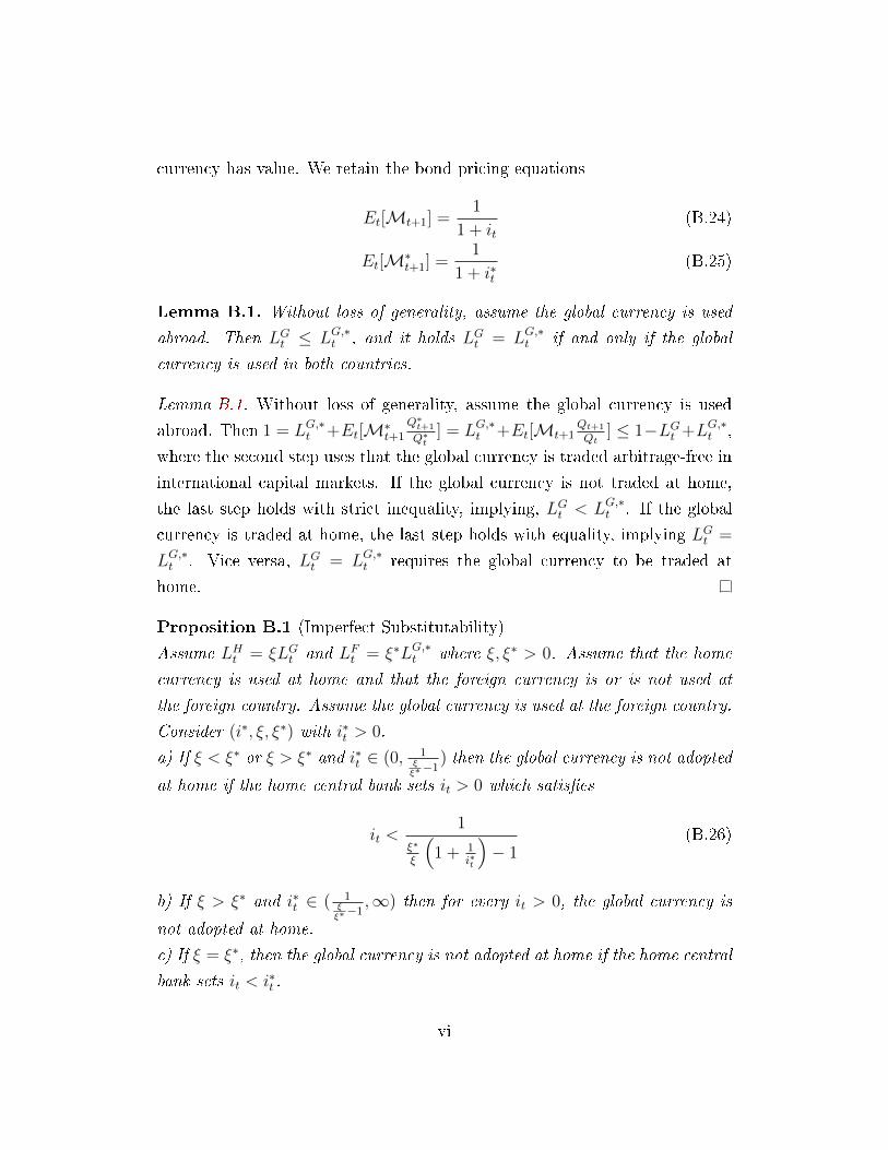
currency has value. We retain the bond pricing equations

Et[Mt+1] =1

1 + it(B.24)

Et[M∗t+1] =

1

1 + i∗t(B.25)

Lemma B.1. Without loss of generality, assume the global currency is used

abroad. Then LGt ≤ LG,∗t , and it holds LGt = LG,∗t if and only if the global

currency is used in both countries.

Lemma B.1. Without loss of generality, assume the global currency is used

abroad. Then 1 = LG,∗t +Et[M∗t+1

Q∗t+1

Q∗t

] = LG,∗t +Et[Mt+1Qt+1

Qt] ≤ 1−LGt +LG,∗t ,

where the second step uses that the global currency is traded arbitrage-free in

international capital markets. If the global currency is not traded at home,

the last step holds with strict inequality, implying, LGt < LG,∗t . If the global

currency is traded at home, the last step holds with equality, implying LGt =

LG,∗t . Vice versa, LGt = LG,∗t requires the global currency to be traded at

home.

Proposition B.1 (Imperfect Substitutability)

Assume LHt = ξLGt and LFt = ξ∗LG,∗t where ξ, ξ∗ > 0. Assume that the home

currency is used at home and that the foreign currency is or is not used at

the foreign country. Assume the global currency is used at the foreign country.

Consider (i∗, ξ, ξ∗) with i∗t > 0.

a) If ξ < ξ∗ or ξ > ξ∗ and i∗t ∈ (0, 1ξξ∗−1

) then the global currency is not adopted

at home if the home central bank sets it > 0 which satis�es

it <1

ξ∗

ξ

(1 + 1

i∗t

)− 1

(B.26)

b) If ξ > ξ∗ and i∗t ∈ ( 1ξξ∗−1

,∞) then for every it > 0, the global currency is

not adopted at home.

c) If ξ = ξ∗, then the global currency is not adopted at home if the home central

bank sets it < i∗t .

vi

Proof. Assume, the global currency is used at the foreign country. The previ-

ous Lemma B.1 jointly with the bond pricing equations yield that the global

currency is not used at home if

0 < LG,∗t − LGt =1

ξ∗LFt −

1

ξLHt (B.27)

≤ 1

ξ∗

(1− 1

1 + i∗t

)− 1

ξ

(1− 1

1 + it

)(B.28)

=1

ξ∗

(1

1 + 1/i∗t

)− 1

ξ

(1

1 + 1/it

)(B.29)

which is equivalent to requiring

1/it >ξ∗

ξ(1 + 1/i∗t )− 1 (B.30)

Case 1: Assume ξ < ξ∗. Then for all i∗t > 0: 1i∗t> 0 > ξ

ξ∗− 1 and thus

ξ∗

ξ(1 + 1

i∗t)− 1 > 0. Thus, the right hand side of (B.30) is strictly positive and

the inequality (B.30) can only hold for it satisfying (B.26). In that case, the

global currency is not adopted at home.

Case 2: Assume ξ > ξ∗.

Case 2a: Assume in addition i∗t ∈ (0, 1ξξ∗−1

). Then, again, the right hand side

of (B.30) is strictly positive and the inequality (B.30) can only hold for it

satisfying (B.26). In that case, the global currency is not adopted at home.

Case 2b: Assume ξ > ξ∗ and i∗t ∈ ( 1ξξ∗−1

,∞). Then, the right hand side of

(B.30) is negative. Therefore, every it > 0, satis�es B.30. Thus, for every

i > 0 the global currency is not adopted at home.

Case 3: For ξ = ξ∗, then inequality (B.30) simpli�es to

1/it > 1/i∗t (B.31)

So that the global currency is not adopted at home for every it < i∗t .

vii