EPRU Working Paper Series - CORE

EPRU Working Paper Series Economic Policy Research Unit Department of Economics University of Copenhagen Studiestræde 6 DK-1455 Copenhagen K DENMARK Tel: (+45) 3532 4411 Fax: (+45) 3532 4444 Web: http://www.econ.ku.dk/epru/

What Drives Sector Allocation of Foreign Direct Investment in Iceland?

Helga Kristjánsdóttir

2005-08

ISSN 0908-7745 The activities of EPRU are financed by a grant from

The National Research Foundation

CORE Metadata, citation and similar papers at core.ac.uk

Provided by Research Papers in Economics

https://core.ac.uk/display/7051747?utm_source=pdf&utm_medium=banner&utm_campaign=pdf-decoration-v1

http://www.econ.ku.dk/epru/

What Drives Sector Allocation ofForeign Direct Investment in Iceland?∗

Helga Kristjánsdóttir†

University of Iceland and EPRU

August 2005

Abstract

The objective of this paper is to examine how the driving forces of in-vestment in a small country like Iceland differ from those in larger countries.Special attention is given to the dominating investment sector in Iceland dueto its resource intensity. Estimates are based on 1989-1999 panel data onforeign direct investment in various sectors. This may help explain why theinvestment pattern in Iceland differs from the general case.

Keywords: Foreign Direct Investment, Multinational Corporations.JEL Classifications Codes: F21, F23

∗I wish to thank for helpful comments by Thorvaldur Gylfason, Ronald B. Davies, JamesR. Markusen, Mette Ejrnæs, Martin Browning and Helgi Tomasson. This paper was writtenduring my stay as a researcher at EPRU (Economic Policy Research Unit) at the University ofCopenhagen, where I took part in a research network on ”The Analysis of International CapitalMarkets: Understanding Europe’s Role in the Global Economy”. The network was funded bythe European Commission under the Research Training Network Programme. The activitiesof EPRU are financed through a grant from the Danish National Research Foundation. Thehospitality of EPRU is gratefully acknowledged.

†Address for correspondence: Helga Kristjánsdóttir, Faculty of Economics and Business Ad-ministration, University of Iceland, 101 Reykjavík, Iceland. Phone +354 551 1718, fax +354 5511718, e-mail: [email protected]

1 Introduction

Foreign direct investment (FDI) has played an important role in the economic devel-

opment of many countries and proven to be an engine of economic growth (Grosse,

1997). Not only does FDI provide capital for development, but it also diversifies

the capital base of countries. It is important for a small country like Iceland, in

need of a more diversified economy, to attract FDI in order to sustain economic de-

velopment and growth. FDI is generally believed to fuel economic growth, however

a recent study by Gylfason and Zoega (2001) shows that economic growth may be

hindered by the crowding out of physical and human capital by natural resource

capital. Moreover, an interesting study by Alfaro et al. (2001) finds economic

growth to be promoted by FDI in economies with sufficiently developed financial

markets. The nature of FDI in Iceland seems to differ somewhat from FDI in other

countries; in the third thesis paper, FDI in Iceland is found to flow particularly

into one sector, the power intensive sector. Because of this, it is important to see

to what extent natural resources drive Icelandic FDI and what factors lead to the

diversification of this FDI across sectors.

A popular approach when analyzing the determinants of FDI is to apply the

factor proportions hypothesis as to consider FDI dependence on factor endowments

such as source and host country differences in skilled and unskilled labor. However,

for small resource based economies like Iceland, the dependence on skilled and

unskilled labor may not be the right endowment approach. Instead, resource based

endowments need to be brought into the picture in order to reflect on the country’s

heavy dependence on marine and hydropower resources.

Anecdotally, the investment dominance of the sector incorporating power in-

tensive industries is generally attributed to the smallness of Iceland, the nature

of its natural resources (its natural resources composition), and how distant it is

from other countries. In another paper by Kristjánsdóttir (2004c), driving forces

for Icelandic FDI are found to be different from the general case when applying

the Knowledge Capital (KK) model specification presented by Carr, Markusen and

1

Maskus (CMM, 2001). But does this help explain why the sectorial composition

of Icelandic FDI seems to differ from other countries?

The objective of this paper is to seek a clearer explanation for this by further

analyzing the sectorial decomposition of FDI. This paper is meant to explain the

relative contribution of various sectors to foreign direct investment. One of the

reasons for choosing the sectorial approach is to differentiate the power intensive

sector from other sectors. This is comparable to a recent paper by Waldkirch

(2003) where he seeks to explain heavy reliance of FDI in one particular industry

in Mexico. However, Iceland differs from Mexico in various ways such as by size,

location, and stage of development.

According to the factor proportions hypothesis, multinationals seek to integrate

production vertically across borders in order to take advantage of different factor

prices resulting from relative differences in factor supplies between countries. The

factor proportions hypothesis has been a dominant explanation of multinational ac-

tivity within conventional trade literature (Helpman, 1984; Helpman and Krugman,

1985).

Since factor abundance is critically linked to factor intensity that may vary

across industries, one goal of this paper is to analyze whether the factor proportions

hypothesis can help explain the sectorial composition of FDI. CMMuse skilled labor

percentages to represent factor abundance in the KK model specification.

Both the work of CMM and subsequent studies find that this is indeed important

for aggregate FDI levels. This paper offers a refinement of CMM’s KK model by

incorporating measures for small economic sizes in population and gross domestic

product (GDP) along with adding natural resource endowments to the conventional

specification. The result supports the hypothesis that there are more factors at

work than the two factors of skilled and unskilled labor in the basic specification.

Furthermore, this approach allows me to discuss how factor abundance may in-

fluence the allocation of FDI across sectors. In particular the relation between FDI

and electricity prices may influence the predominance of FDI in the Icelandic power

intensive industry. Also, by sectorial disaggregation, it is possible to determine

2

how the economic size variables in the CMM specification affect individual sectors.

Economic size is highly relevant in this paper, not only because the source countries

are considerably larger than the host country Iceland, but also because during the

research period a large part of FDI comes from one particular country, Switzer-

land. The dominance of Switzerland brings us back to the discussion on electricity

prices, hydropower and the power intensive industry. Switzerland has a history of

being specialized in using hydropower, as a natural resource, to generate electricity

for power intensive industries like the aluminum industry. However, in the 1990s

Switzerland had almost fully exploited its hydropower production potential (Czisch

et al., 2004, pp. 8-3). Thus Swiss firms may have been especially intensive in

hydroelectric power and actively seeking more of it. A prime example of this is

AluSwiss, a Swiss headquartered multinational enterprise (MNE), which undertook

greenfield investment in an aluminum smelter in Iceland in the 1990s. Overall,

Icelandic foreign direct investment in power intensive industries greatly increased

in the 1990s. Thus one of my goals is to determine how hydropower electricity

prices affects FDI in the power intensive industries. This is in addition to the

standard analysis of how skill differences between the source and the host country

affect FDI.

Also, since fishing is very important to the Icelandic economy, I include the total

fish stock caught in Icelandic waters in order to control for this factor. Moreover,

issues such as infrastructure, pollution quotas, and fish catch are accounted for in

this research. Since Iceland has a considerably larger pollution quota than all

other countries engaging in the 1997 Kyoto Protocol on climate change, this may

well affect the sector allocation of FDI.

The estimates obtained in this paper are based on unique FDI panel data on

investment sectors in Iceland. The FDI data cover investments made by 17 source

countries over a period of 11 years. The FDI is classified into 4 major sectors.

These are as follows: power intensive industries (as sector 1), Commerce and Fi-

nance (sector 2), Telecom and Transport (sector 3), and finally Other industries

(sector 4). More specifically the fourth sector accounts for the following indus-

3

tries: Manufacturing, Agriculture and Fishing, Mining and Quarrying, and other

industries. Estimates are obtained for sector shares of country’s FDI as well as

levels of FDI in each sector, since FDI shares reflect the relative size of each sector

within a particular year of investment. The application of sector shares allows for

analyzing the relative importance of the power intensive sector compared with other

sectors. An example of an application of FDI share proxy can be found in a paper

by Brainard (1997). Brainard uses outward shares of U.S. sales to proxy FDI sector

shares. In the case of Brainard, it is reasonable to apply shares of U.S. affiliate sales

abroad as a proxy for outward FDI, rather than applying actual FDI data, because

a considerable amount of U.S. outward FDI is derived from mergers and acquisi-

tions. However, in the case of Iceland it is more reasonable to capture FDI with

actual FDI, since Iceland has a short history for FDI, and FDI in the dominating

power intensive industry has primarily been in the form of greenfield investment.

In a related manner, Slaughter (2000) constructs an investment share variable as

the share of ”majority owned affiliates” in overall multinational investment.

Finally, one notable feature of the data is the large number of zeros, i.e. countries

that do not invest in a particular sector. Because of this, I control for whether

sample selection is driving my results, by using the Heckman’s (1979) two-step

procedure. In particular, since the theories of FDI assume a crucial role for fixed

cost in determining whether FDI occurs, these final results provide some potential

insights into this issue in a manner heretofore unexplored.

The paper is organized as follows. In Section 2 the model is laid out. Section 3

gives an overview of the data used in this research. Section 4 contains quantitative

results from the sectorial decomposition. In Section 5 results from using a sample

selection are introduced. Finally, conclusions are presented in Section 6.

4

2 Model Specification

The main issue of concern in this paper is to capture the driving forces behind

investment incentives across sectors. In other words, to see whether it is pos-

sible to capture sector specific determinants of foreign direct investment. In an

earlier paper (Kristjánsdóttir, 2004), I provide analysis on how the CMM (2001)

specification performs for small countries like Iceland. A potential reason for the

specification’s poor results could be the dominance of one sector, the power intensive

sector. Therefore, the objective here is to refine to the baseline CMM specification

in order to allow for decomposition of FDI, and to determine what drives sector

specific FDI.

I do this in two ways. One is adding factors such as natural resources to an

improved version of the CMM specification in order to adjust the model to a resource

based host country like Iceland. Thus, this is akin to the empirical trade literature

that found it necessary to bring in more factors in order to resolve Leontief’s classic

critique of the Heckscher Ohlin factor proportions theory. Potentially because the

CMM specification is designed to capture the effects of the level of skill on FDI,

rather than effects of natural resources .

The breakdown of industries reveals that CMM performs differently for different

sectors, although overall it still does not perform as expected. This leads me to a

gravity approach similar to that used in my earlier paper (Kristjánsdóttir, 2004b).

The motivation for estimating individual sector shares is obtained from Brainard

(1997). In her paper, Brainard applies ”the share of affiliate sales accounted for by

exports”...that is the...”share of exports in total sales” (Brainard, pp. 528)1. This

corresponds to capturing the share of non-affiliate sales in total sales. Brainard is

thereby able to use an inverse proxy for the share of FDI in foreign MNEs activities2.

1Markusen (2002, pp. 409) says the following about the index used by Brainard in her 1997 pa-per: ”The intra industry affiliate sales index measures the degree of international cross-investmentin a particular industry: production and sales abroad by US MNEs and production and sales inthe United States by foreign MNEs”.

2Outward affiliate sales relative to exports and inward affiliate sales relative to imports for 64industries in the United States are given in Brainard (1997).

5

The idea of using export shares is based on a similar argument as the one presented

in this paper. However, in this paper the objective is to capture the sector shares

of FDI. This is done by presenting the relative weight of sectors in those years

when some investment takes place. One of the advantages of measuring sectorial

FDI in shares, rather than levels, is that it reflects the relative weight of individual

sectors. The way the model specification for shares is set up reflects the relative

amount of investment made within each year, no matter the actual size of FDI.

Thus, even when there is little total FDI (as is often the case in small countries

like Iceland) I can extract information from the data.3

An example using capital stock share to construct the dependent variable can

be seen in Slaughter (2002). Slaughter calculates the share of MOFAs4 in overall

MNEs investment (Slaughter, 2002, pp. 457), whereas here the estimates are based

on the share of sectorial FDI in overall FDI. Slaughter places the share of skilled

labor on the left hand side of the equation, and the share of capital stock on the

right hand side5. In my case, the share of capital stock is placed on the left hand

side, and skilled labor on the right hand side following the exogenous endowment

literature precedent.

When formulating the model specification, I start by choosing the share of FDI

stock to be the dependent variable. The basic equation specification can be esti-

mated as follows:

3Brainard (1997) believes that use of the share measure ”should mitigate some of the concernabout industry - country pair effects”. This reasoning applies to my paper because I also dealwith industry-country pairs, which may vary a lot in the amount they invest. CMM need not todeal with this issue in their paper, since they use time series data for countries and years. In hispaper, Slaughter (2002, pp. 454), says that he uses shares ”Because shares offer a rough controlfor some of these other forces acting MNE-wide I mostly focus on the share data. I interpretrising shares of affiliate activity to be evidence of MNE transfer.”

4MOFA refers to majority-owned affiliates in which parent MNEs hold at least 50% stake. Incomparson, FDI generally refers to at least 10% ownership of a single parent MNE.

5The dependent share variable used by Slaughter is based on the skilled labor share in the totalwage bill. More specifically, he captures the share of skilled labor in the overall labor force bydeviding the wage of nonproduction workers (referred to as skilled labor) by the total wage bill toproduction and nonproduction workers.

6

SHAREi,s,t ≡ Fi,s,t

Fi,t

= β0 + β1Ysumi,t + β2Ydiff2i,t + β3Sdiffi,t (1)

+β4Ydiffi,t∗Sdiffi,t + β5Invct + β6Tct

+β7Tct∗Sdiff2i,t + β8Tci,t + β9Disi + εi,s,t

In Equation (1) the dependent variable SHAREi,s,t represents investment share

of a particular sector s in particular year t by source country of investment i.

Equation (1) has an error term εi,t with E[εi,t | xi,t] = 0, where xi,t represents

the explanatory variables in the equation6. Note that because it is created from

stock data, the dependent share variable represents sector specific FDI divided by

accumulated investment. More specifically the dependent variable SHAREi,s,t is

defined as Fi,s,t divided by Fi,t, conditional on Fi,t > 0. The share of FDI in a

particular sector7 is calculated as FDIi,t =Pn

s=1 FDIi,s,t where s runs from 1 to n

, and n equals 4.

The explanatory variables on the right hand side of the first regression equation

are the same as in the CMM model specification. I start out by including all the

variables in the CMM model, and then apply some data-driven refinements. The

first variable in Equation (1) is Ysumi,t representing the sum of the source and host

countries’ GDP. The variable coefficient is typically expected to be positive, since

more investment is believed to take place with an increase in the economic size of

the source and recipient country. The second explanatory variable represents the

absolute size difference Ydiff2i,t of source and host countries’ GDP. The coefficient

sign is expected to be negative, since less investment is expected to take place as

size difference increases. The literature on horizontal multinational activities, e.g.

by Markusen (1984), explains well why more FDI is believed to take place between

countries of similar economic size.

According to the factor proportions hypothesis, multinationals take advantage

6The coefficient estimates are therefore consistent, although not efficient.7The share observations do not include the years when no FDI takes place.

7

of factor price differences by fragmenting production vertically across countries de-

pendent on difference in relative factor supplies. Factor price differences give rise

to vertical FDI (Helpman, 1984). Here, I include skill differences which are meant

to account for difference in relative factor endowments. An analogous variable is

used by CMM (2001). FDI is expected to increase as the source country’s labor

force becomes increasingly more skilled relative to host, and therefore the variable

has a positive expected coefficient sign. A term Ydiffi,t∗Sdiffi,t is also includedto capture the interaction between size and skill differences. The interaction term

reflects the importance of skilled labor differences, depending on the magnitude of

GDP differences between the source and host country. Furthermore, variables for

trade costs and investment costs are included in the model. The motivation for

including variables for trade and investment costs is to determine how investment

is affected by restrictions of this type. An increase in investment costs of the

host country Invct is expected to decrease investment in the host. An increase in

the host country’s trade costs Tct is expected to trigger FDI, since then the source

country is likely to prefer investment to costly trade. On the contrary, an increased

trade cost in the source country Tci,t is believed to decrease its interest in investing

in the host, since it becomes more costly for the source to import from overseas

affiliates. Moreover, the interaction between skill differences and trade cost of the

host Tct∗Sdiff2i,t indicates the relevance of absolute skill differences, depending onthe magnitude of trade costs in the host country. The higher the trade cost, the

more important the skill differences. The variable coefficient is expected to have a

positive sign.

The last variable in Equation (1) represents distance. Distance can be regarded

to be a proxy for transport costs and associated transaction costs. The inclusion

of distance to explain investment is well known in literature on FDI (CMM 2001;

Jeon and Stone, 1999; Bergstrand, 1986). FDI is believed to decrease as distance

between the source and host countries increases, and therefore the coefficient sign

is expected to be negative.

In latter sections of this paper, some extensions of the basic model specification

8

are used, including some additional control variables. These control variables are

not in the model specification presented by CMM. First of all, I use a variable

accounting for the catch in Icelandic waters. The main reason for including this

variable is that it captures fluctuations in what has been referred to as the main nat-

ural resource of Iceland, the fish stock obtainable from the fishing grounds around

the country. When the catch is large, this may draw labor or other resources from

FDI. Furthermore this effect may vary across types of FDI. The variable Catcht

represents an index of the total fish catch in the host country Iceland. More specif-

ically the variable is defined as ”Total catch at fixed prices, Seasonal adj. Indices”.

The index runs through the whole estimation period from 1989 to 1999, where 1995

has been set as a base year with a value of one. The catch variable is obtained

from the National Economic Institute of Iceland. The second control variable used

in this paper is INFdiffi which represents difference in infrastructure between the

source and the host country in 1999. More specifically the variable can be presented

as INFdiffi ≡ (INFi−INF). All variables that represent differences between thesource and host country are presented as the source country value minus the host

country value. I use infrastructure to reflect host country competitiveness, partly

because countries endowed with natural resources for the power intensive industry

often suffer from poor infrastructure. These would for example be some of the

African and South American countries. Furthermore, for multinationals seeking

a power plant location, the strength of the infrastructure in Iceland can play an

important role. This infrastructure measure is obtained from the World Competi-

tiveness Yearbook 2000. The yearbook ranks countries by ”competitiveness input

factors”, where infrastructure is one of them. Countries listed in the yearbook

run from 1 to 47, with 1 being the most competitive country. By pooling a range

of different competitiveness factors together, an overall competitiveness index is

formed8. An increase in the INFdiffi variable indicates that the host country

has increasingly less infrastructure, which may or may not increase FDI in the host

8Iceland was listed as the 17th most competitive country in 1999, moving up from being number19 in 1998.

9

(Iceland). Therefore the coefficient sign can be expected to be either positive or

negative. Table 1 provides an overview of the variables used in this paper.

Table 1. Variable Definition

VariableExpectedsigns

Sharei,s,tShare of foreign direct investment (FDI) made by the

source country (i) in the host country (j), in sector

(s), over time (t).

Fdii,s,tForeign direct investment made by source country (i)

in the host country (j), in sector (s), over time (t).

Ysumi,t

The sum of the Gross Domestic Product (GDP) of

the source country (i) and the GDP of the host coun-

try (j), over time (t).+

Ydiff2i,tThe GDP of the source country (i) minus the GDP

of the host country (j), squared over time (t).—

Sdiffi,tSkilled labor in the source country (i) minus skilled

labor in the host country (j), over time (t).+

Ydiffi,t∗Sdiffi,tInteration term, capturing the interaction between

the GDP difference of the source and host countries

and the skill difference variable, over time (t).—

InvctThe investment cost foreign investors are faced with

when investing in the host country (j), over time (t).—

Tct Trade costs in the host country (j), over time (t). +

Tct∗Sdiff2i,tInteraction term, capturing interaction between

trade costs in the host country and squared skill dif-

ferences, over time (t).+

Tci,t Trade cost in the source country (i), over time (t). —

DisiGeographical distance between the source country (i)

and the host country (j), in kilometers.—

CatchtThe ”total catch index” for the host country, Iceland.

The index represents development in overall catch in

Icelandic waters. With 1995 as a base year.+

INFdiffiInfrastructure index differences between the source

country (i) and the host country (j), in 1999.+/—

POLLdiffiPollution Quota differences between the source coun-

try (i) and the host country (j). Based on the 1997

Kyoto Protocol.—

GMTSTdiffi,tGovernment Stability differences between the source

country (i) and the host country (j).+/—

Two more control variables are applied in the basic KK model specification,

these are POLLdiffi and GMTSTdiffi,t. The variable POLLdiffi represents

10

the difference in pollution quota in the source and host country. The data are

classified as ”Quantified emission limitation or reduction commitment”, (percentage

of base year or period) and obtained from the Kyoto Protocol to the United Nations

Framework Convention on Climate Change9. The Third Kyoto session was signed

in December 199710. An increase in pollution difference of the source and host

country indicates an increase in the pollution quota of the source relative to the

host. An increase in this type of pollution quota is likely to diminish investment in

pollutive industries in the host country, such as the power intensive industry. The

measures for government stability refer to both countries and time, and the variable

is denoted as GMTSTdiffi,t. Higher numberical value for stability is interpreted

as a more stable economy. These Government Stability data are the year beginning

data, however the data for Germany run only from 1991 (since German unification).

This variable is meant to reflect the relative stability of the Icelandic government,

where and increase in difference can be expected to either stimulate or hinder FDI.

The government stability data is obtained from the International Country Risk

Guide.

9What is of interest in this protocol is that Iceland has highest quota of all countries listed.10More information on the Kyoto Protocol are to be found in Appendix B.

11

3 Data

The database on FDI and the share of FDI in various sectors in Iceland covers

investments made by the main source countries of investment in Iceland over the

time period 1989-1999. In order to give a taste of what is in the data, Table 2

classifies the sample countries by their share in overall FDI in Iceland. There are

17 source countries in the sample which account for about 99% of total FDI11.

The percentage shares presented in Table 2 indicate that there is a substantial

difference in the amount of investment made by various countries, with Switzerland

being the main source country of foreign direct investment.

Table 2. Major Source Countries of FDI (1995 US dollars).

The Countries Reported Account for the Biggest Part of FDI.

Switzerland 1,095,079,000 Sweden 65,178,950

United States 485,395,200 Luxembourg 58,259,560

Denmark 213,626,400 Germany 43,424,390

Norway 191,819,600 Finland 11,947,020

United Kingdom 112,070,400 Belgium 9,159,265

Japan 65,231,580 Netherlands 4,879,091

Source: Central Bank of Iceland.

The second major source country of investment in Iceland is the United States,

with Denmark being the third. The sample countries with the least amount of

investment in Iceland are Australia, Canada, Spain, Austria, and France. These

countries are not displayed in Table 2, but are still used in estimation.

Table 3 exhibits the share of each sector in overall investment over the period of

estimation. The sector disaggregation is as follows: the power intensive industry as

sector 1, commerce and finance industry as sector 2, the telecom industry and the

transport industry as sector 3, and finally sector 4 accounts for all other industries.

More specifically, sector four accounts for the following industries: manufacturing,

agriculture and fishing, mining and quarrying and other industries.11Countries accounting for the remaining investment are: Chile, Faeroe Islands, Gibraltar, Israel,

Latvia, Russian Federation.

12

Table 3. Decomposition of FDI in Iceland (1995 US dollars).Sector Allocation of Industries

Sector 1 - Power Intensive 1,524,921,000

Sector 2 - Commerce- Finance

468,544,300

Sector 3 - Telecom- Transport

50,800,210

Sector 4 - Manufacturing- Other

316,047,200

Total 2,360,312,710

Source: Central Bank of Iceland

Due to the low overall FDI, the procedure is to decompose investment into a

few main subsectors. When doing this, it is logical to separate the power intensive

industry from the others due it its size. Subsequently, following previous research,

the sectors are now classified with Commerce and Finance as sector 2, and Telecom

and Transport12 as sector 3. Sector 4 is primarily Manufacturing. However, Agri-

culture, Fishing, as well as Mining and Quarrying are classified with manufacturing,

but these are a very small part of FDI. Together Agriculture, Fishing, and the Min-

ing and Quarrying sector accounted for less than 2.5% of total FDI. It is worth

noting that even though there is very small FDI in Fishing, the Fishing industry

has been a dominant domestic industry in Iceland in the last several decades.

The numbers presented are inward stocks of FDI in Iceland, represented in 1995

US dollars. Data on FDI stock in Iceland are obtained from the Central Bank of

Iceland. In a recent paper by Davies (2002), the advantages of using FDI stock are

12More specifically, the sector classification is often times ”Transport & Communication” (GuoJu-e, 2000), but I found it to be more direct to call it ”Transport & Telecom”.

13

well explained, as well as the reason it can be more applicable than FDI flows or

affiliate sales representing multinational activities. Data on the level as well as the

share of FDI are kindly provided by the Central Bank of Iceland.

Table 4. Summary Statistics

Variable Units Obs Mean StD. Min Max

Sharei,s,t Index [0,1] 568 0.25 0.39 0 1

Fdii,s,t Million USD 748 3.16 13.89 -0.95 157.9339

Ysumi,t Trillion USD 740 1.23 1.96 0.02 8.59

Ydiff2i,t 740 5.29 13.78 0.00005 73.51

Sdiffi,t Index [-1,1] 516 0.03 0.06 -0.08 0.14

Ydiffi,t∗Sdiffi,t 516 0.04 0.22 -0.27 1.11

Invct Index [0,100] 340 33.01 1.92 29.92 35.28

Tct Index [0,100] 340 48.18 3.79 43.7 52.50

Tct∗Sdiff2i,t 260 0.18 0.25 0.00002 0.85

Tci,t Index [0,100] 748 27.88 11.18 5.30 64.80

Disi Million Kilometers 748 0.004 0.004 0.002 0.02

Catcht Fish Quota Index 748 1.01 0.04 0.92 1.07

INFdiffi Compet. Index 748 -1.76 6.44 -11 10

POLLdiffi Poll. Quota Index 748 -0.16 0.04 -0.18 -0.02

GMTSTdiffi,t Govmt Stab. Index 740 -0.09 1.49 -4 5

Sources: Central Bank of Iceland, Economic Institute of Iceland, Distance Calculator, Inter-

national Labor Organization, World Bank, World Competitiveness Report, Kyoto Protocol.

Table 4 represents an overview of the overall sample, where the total number of

observations is the multiplication of the 17 countries, 4 sectors and 11 years.

In his paper, Slaughter (2002, p. 454), says that he uses shares ”Because shares

offer a rough control for some of these other forces acting MNE-wide I mostly focus

on the share data. I interpret rising shares of affiliate activity to be evidence of

MNE transfer.”

Data on GDP, both in sum and squares, are taken from the World Bank CD

Rom (2002), and are in constant 1995 US dollars. Data on GDP in Germany in

14

1989 and 1990 are not included here, since these are the years before the unification

of Germany. Data on investment and trade costs are obtained from theWorld Com-

petitiveness Report and data on distance comes from the Distance Calculator. The

quota index for the catch variable is obtained from the former Economic Institute

of Iceland. Data on Infrastructure are obtained from the World Competitiveness

Yearbook 2000. Data on pollution quotas come from the Kyoto Protocol (1997) in

the section on country-by-country emission targets. The government stability data

is obtained from the International Country Risk Guide (ICRG), published by The

PRS Group on Government Stability13. All regressions results are obtained using

STATA version 7.0.

13More specifically it is taken from: Political Risk Points by Component, Table 3B.

15

4 Estimation Results

4.1 FDI Shares, Basic Specification

This section provides us with results for shares of individual sectors. In the standard

models, there are generally two sectors: an FDI sector x and a numerarie sector

y. In reality, a single FDI sector x is really several sectors in which there is FDI.

Here, I analyze four such sectors, i.e. I decompose x into x1, x2, x3, and x4.

An overview of the regression results for the CMM specification in Equation (1)

as shown in Table 514.

Table 5. CMM Specification for Sector Shares

Sector 1 Sector 2 Sector 3 Sector 4 S. 2 to 4

Regressors Power

inten.

Com.

& Fin.

Tel. &

Trans.

Oth.

Ind.

Ysumi,t −0.29∗∗∗(−4.59)

0.13(0.94)

0.19(1.49)

−0.03(−0.42)

0.09(1.30)

Ydiff2i,t 0.05∗∗∗(4.02)

−0.02(−0.94)

−0.02(−0.88)

−0.004(−0.25)

−0.02(−1.12)

Sdiffi,t −1.19(−0.66)

−3.78(−1.52)

2.71(1.19)

2.26(1.23)

0.39(0.28)

Ydiffi,t∗Sdiffi,t −0.56(−1.39)

0.63(1.12)

−0.21(−0.37)

0.15(0.34)

0.19(0.51)

Invct 0.001(0.03)

−0.01(−0.27)

0.02(0.80)

−0.01(−0.47)

−0.0004(−0.01)

Tct −0.009(−0.53)

−0.001(−0.04)

0.0002(0.01)

0.009(0.63)

0.003(0.23)

Tct∗Sdiff2i,t 0.10(0.30)

0.04(0.09)

−0.54(−1.15)

0.39(0.99)

−0.03(−0.10)

Tci,t 0.03∗∗∗(5.67)

−0.01∗∗∗(−2.71)

−0.008∗∗(−2.08)

−0.004(−0.89)

−0.009∗∗∗(−3.02)

Disi −30.99∗∗∗(−3.71)

−15.39∗(−1.77)

−16.18∗(−1.95)

62.57∗∗∗(7.77)

10.33(0.72)

Constant 0.23(0.35)

1.09(1.43)

−0.47(−0.80)

0.14(0.19)

0.26(0.19)

Observations 57 57 57 57 171

R-squared 0.64 0.39 0.31 0.51 0.09

Note: Robust t-statistics are in parentheses below coefficients. ***, ** and * denotesignificance levels of 1%, 5% and 10% respectively.

14All robust t-statistics are calculated using White’s (1980) heteroskedaticity correction.

16

Some changes in exogenous variables can be important for some sectors and not

others. This is what the research for sector shares tests for. If variable estimates

for an individual sector in Table 5 are insignificant, it does not indicate that chosen

variables do not affect the level of FDI in any sector. What it does indicate is that

the variable in question affects FDI levels in each sector in roughly a proportional

fashion. If this were true for all variables, then the standard way of estimating

FDI (aggregating across sectors and using a single FDI variable) might be sufficient.

What this approach adds to the debate is that the standard approach may overlook

important heterogeneity across sectors. Furthermore, this indicates that the factor

proportions hypothesis can be important even within what is typically called x, i.e.

it can affect x1 and x2 differently.

In Table 5, the first two size variables are estimated to be significant, however

with coefficient signs different from what is predicted by the theory. The negative

coefficient of the first variable indicates that the share of the power intensive sector,

in overall investment, decreases with an increase in the sum of the economic size of

the host and the source country. When the investment weight of small countries in

Table 2 is considered, especially Switzerland, these results need not be surprising.

As for the second variable, a positive coefficient indicates that as the squared dif-

ference between the source and host country increases, FDI in sector one increases

relative to other sectors. Taken together the results for the first two variables

are somewhat puzzling, since it seems as they go against each other. One way of

interpreting this is to say that the share of sector one, in overall FDI, is negatively

affected by an increased in the size of the source countries; however the relationship

can be regarded as increasing based on the positive sign of the latter size variable,

so that the relationship is negative but increasing15. Estimates for sectors 2 to 4

indicate that the coefficient signs for the first two size variables have signs opposite

from that which is obtained for the first sectors. This indicates that forces driving

15This interpretation refers to the fact that the variation in the size variables is primarily dueto variation in the size of the source country, since almost all source countries are considerablelarger than the host country, Iceland.

17

investment in sectors 2 to 4 are of different nature from those driving investment

in the first sector. What is interesting is that economic size is only estimated to

be of significant importance in the case of the power intensive industry, not other

industries.

The results obtained for distance indicate that an increase in distance of 1 million

kilometers is predicted to decrease the share of the power intensive sector one by

about 31%, or (based on the average distance measures in Table 4) a more realistic

thing would be to say that a distance increase by 100,000 would result in a 3%

decrease in sector one investment16.

In Table 5 foreign direct investment (FDI) is disaggregated into four sectors.

These are the power intensive industry in Iceland as sector one, commerce and

finance as sector two, the telephone and transport industries as sector three, and

other industries as sector four17. Finally industries 2, 3, and 4 are aggregated in the

last column. Sector one is not included in last column since by definition the share

of all sectors combined is always one. The addition of sectors 2, 3, and 4, provided

in the last column, is presented to reflect on the interaction between sector 1 and

all remaining sectors. The first column shows estimates for sector one. Overall,

an increase in distance shifts FDI from sectors 1 - 3 into sector 4. It may or may

not increase the level of FDI in any single sector18.

When the skill difference variable Sdiffi,t is considered, it turns out that it

is not found out to be significant (neither when estimated individually, nor when

estimated as an interaction term with other variables)19.

16Note that all inference assums normality, thus the usual caveats to this discussion apply.17More specifically sector four accounts for the following industries: Manufacturing, agriculture,

fishing, mining and quarrying and other industries.18For example in Table 6 in Kristjánsdóttir (2004c), it could be that distance has a negative

coefficient across the board, which it does. This means that an increase in distance decreasesFDI in all sectors.19A potential way to analyze the skill variable further would be to apply the same procedure

as Markusen and Maskus (MM, 2002). MM include skill differences in two interaction terms,accounting for the cases seperately when skill differences are positive and negative. This approachhas the advantage that only two more degrees of freedom are lost, when compared to the CMMmodel. However, the approach applied by Blonigen, Davies and Head (BDH, 2003) involves amuch greater loss of degrees of freedom, since it implies a division of the sample to two subsamples,depending on the whether skill differences are positive or negative.

18

When it comes to the variables for host country investment cost Invct, and

host trade cost Tct as well as the interaction between trade cost host and skill

differences Tct∗Sdiff2i,t, they are all estimated to be insignificant. Taken togetherthese results may be interpreted such that the variables do not affect FDI allocation

to different sectors. In other words, it can be said that MNEs do not choose one

sector rather than another based on these factors; the sectors are all equally sensitive

to changes in these variables. Recall, however, that FDI levels may change, thus

this is not itself a rejection of the factor-proportions hypothesis.

Let us then consider the variable for trade cost in the source country Tci,t. It

is estimated to be positively significant in the case of sector 1 and negative for

sectors 2 and 3. The positive coefficient can be interpreted such that an increase

in source country trade cost has positive effects on the share of sector one in overall

investment, while the contrary holds for other sectors. One way of interpreting these

results is to say that only for sector one does high trade cost trigger investment.

An increase in trade cost in the source country might trigger investment in sector

one only if the goods produced by the power intensive sector are not faced with

conventional trade costs when shipped back home. This possibility is explored in

Section 5.

Finally, the distance variable is estimated to be significantly negative for sectors

1 through 4. This greater distances seem to hurt FDI in these industries relative

to the manufacturing heavy sector 4.

The last column accounts for sectors 2, 3, and 4, and the number of observations

in the last column is the sum of observation number for 1-3 sectors. The estimates

obtained for the regression in the last column are insignificant, except the source

trade cost, consistent with the regressions on sectors.

Many of the variables are estimated to be insignificant in Table 5. Therefore, it

is interesting to continue the research by estimating levels of FDI, since the CMM is

designed for level estimates and therefore has potential to do better for levels than

shares. Furthermore, these results describe relative shares across sectors, which

leaves out potential information regarding levels of FDI in each sector.

19

5 FDI Levels, Tobit Estimates

I next investigate the degree to which sectorial FDI can be explained, when pre-

sented in levels, rather than shares of FDI like before. By doing so, it is possible

to capture the effects of the CMM specification variables on actual levels of FDI.

Table 6. Tobit Estimates for the CMM Model Specification

Sector 1 Sector 2 Sector 3 Sector 4 S. 2 to 4

Regressors Power

inten.

Com.

& Fin.

Tel. &

Trans.

Oth.

Ind.

Ysumi,t −123.43∗(−1.92)

4.54∗∗(2.09)

5.18∗∗(2.18)

−4.85∗∗(−2.09)

0.62(0.35)

Ydiff2i,t 19.69∗(1.92)

−1.10∗∗(−2.01)

0.32(0.38)

1.13∗∗∗(2.67)

0.15(0.45)

Sdiffi,t 323.54(0.57)

−34.94(−1.12)

65.42(0.88)

12.79(0.33)

−1.41(−0.05)

Ydiffi,t∗Sdiffi,t −197.42(−0.81)

85.76∗∗∗(3.32)

−31.29(−0.85)

−8.37(−0.72)

2.50(0.27)

Invct −0.46(−0.06)

0.27(0.59)

−0.07(−0.11)

0.11(0.15)

−0.02(−0.03)

Tct −2.86(−0.64)

0.12(0.52)

0.01(0.04)

−0.62∗(−1.69)

−0.30(−1.03)

Tct∗Sdiff2i,t −147.62(−0.99)

−50.32∗∗∗(−4.61)

−4.51(−0.37)

−3.65(−0.44)

−6.23(−0.94)

Tci,t 7.24∗∗∗(4.81)

−0.18∗∗∗(−2.98)

−0.34∗∗(−2.24)

−0.22∗∗(−1.98)

−0.21∗∗(−2.49)

Disi −25, 621.77(−1.12)

−6, 422.14∗∗∗(−4.87)

−11, 896.84∗(−1.91)

−246.68(−0.91)

−601.06∗∗(−2.27)

Constant 58.77(0.32)

9.17(1.01)

25.50(1.55)

33.59∗∗(2.33)

19.97∗(1.72)

Total Obs. 65 65 65 65 195

Left cens.obs. Fdi≤0 47 29 50 21 100

Uncen. obs. 18 36 15 44 95

PseudoR-sq.

0.21 0.29 0.38 0.17 0.07


20

In Table 6 the results for level estimates are presented. The main difference

between estimating shares or levels of FDI is that the level estimates allow us to

determine the direct variable effects on the level of investment, while share estimates

indicate how the share of FDI in individual sectors is determined.

By presenting FDI in levels rather than shares, estimates for individual sectors

are independent of estimates for other sectors. In Table 6 the Tobit estimates for

individual sectors are introduced. The row labelled ”left censored” observations in

Table 6 represents those observations that are zero or negative. The left censored

observations are in most cases zero values20, since the observations are rarely neg-

ative21. There is a higher number of left censored observations in sectors 1 and 3

than there is in sectors 2 and 4. This is as could be expected, since sectors 2 and

4 are composed of a bigger variety of industries than 1 and 3.

It appears that the size variables continue to have the same signs for sectors 1

and 4 as those in Kristjánsdóttir (2004c). This may provide further support for the

hypothesis that estimates for sectors 2-4 combined are crowded out by the power

intensive sector due to the power sector size.

What is also noteworthy in Table 6 is that the skill difference variable is not

estimated to be significant for individual sector FDI. This suggests that skilled labor

differences do not have significant impact on the amount of FDI in individual sectors.

An exception, though, maybe found for sector 2, where both of the interaction

terms are estimated to be significant. The significance of the interaction terms

in the case of sector 2 can be interpreted such that endowments of skilled labor

may be important in the telecom industry, especially during periods of Icelandic

protectionism. What is also of particular interest in sector one is that distance is

not estimated to be significant, indicating that other factors than distance are more

important when multinationals choose to invest in Iceland.

20The Tobit lower limit is set at zero, then negative values are not trucated but accumulatedaround the zero value. The overall results are weak because of how many observations are leftcensored.21However, negative observations are identified in the case of France, UK, Luxembourg, Norway

and Sweden.

21

On the whole however, the CMM specification of the KK model does not seem

to do well either when I estimate FDI in levels, since most of the variables are

insignificant.

There is reason to expect that variation in the power intensive sector may be

driving the results for level estimates of FDI. This is because investment in the

power industry is often a lump sum investment indicative of high fixed costs. Alter-

natively, it may be that the baseline CMM specification ignores important omitted

variables. I investigate this in the next section.

22

6 FDI Levels, Modification of the CMM Specifi-cation

Let us next investigate estimates for an alternative model specification. The new

specification is presented in Equation (2):

Fdii,s,t = β0 + β1Ysumi,t + β2Ydiff2i,t + β3Sdiffi,t (2)

+β4Disi + β5Catcht + β6INFdiffi + εi,s,t

The variables in Equation (2) that are originated in the CMM specification are

the two first variables accounting for economic size, the third variable represents

skills, and the fourth variable distance. The reason for the choice of those particular

variables from the CMM specification is that, for the first thing, determination

of size effects are a key issue in the case of Iceland (due to its smallness) and

distance is also very important (due to the country’s geographical location). Finally

the variable accounting for skilled labor endowments is a crucial variable in the

Knowledge-Capital framework.

Variables for trade costs and investment cost are not included in Equation (2)

for two reasons. First, because there is reason to expect these not to be directly

applicable to inward FDI in Iceland, since the host country trade and investment

cost is estimated to have low significance. Second, although significant, source

country trade cost is not of primary interest for inward FDI in Iceland. Also as

Table 4 in Section 3 reveals, the trade and investment costs together with interaction

terms have the fewest observations of all the variables and therefore act as being

most restrictive.

Two new variables are introduced in Equation (2), these are Catcht which is

an index for fish catch in Icelandic waters, and INFdiffi cross sectional variable

accounting for differences in infrastructure of the source and the host. More specif-

ically, the Catcht variable captures how investment incentives are affected by the

size of available fish stock in Icelandic waters, and infrastructure INFdiffi in Ice-

23

land compared to the infrastructure in source countries (in the year 1999). These

new variables are interesting for the reason that they reflect upon issues concerning

horizontal and vertical foreign direct investment. By incorporating a proxy for the

main natural resource of Iceland, the fishing area, it helps indicate further whether

the sources of FDI are of vertical nature (that is, whether FDI is driven by cheap

access to natural resources, as a form of relative endowments)22. Based on the fact

that FDI in fisheries (fish processing firms and trollers) is prohibited in the period

analyzed, we now want to estimate whether we can identify whether FDI is affected

by the catch variable.

Table 7. New Model Specification for FDI Levels

Sector 1 Sector 2 Sector 3 Sector 4 All Sts

Regressors Power

inten.

Com.

& Fin.

Tel. &

Trans.

Oth.

Ind.

Ysumi,t −22.342∗∗∗(−4.74)

0.934(1.24)

0.588(1.38)

−5.118∗∗∗(−3.19)

−6.485∗∗∗(−3.92)

Ydiff2i,t 3.343∗∗∗(5.21)

−0.095(−1.02)

−0.054(−0.77)

0.949∗∗∗(3.36)

1.036∗∗∗(4.00)

Sdiffi,t −207.470∗∗∗(−3.70)

6.182(0.75)

−0.284(−0.18)

−9.883∗(−1.71)

−52.864∗∗∗(−3.42)

Disi −964.076∗∗∗(−3.83)

−269.435∗∗∗(−5.41)

−57.889∗∗∗(−2.68)

−153.809∗∗∗(−2.88)

−361.302∗∗∗(−5.24)

Catcht −60.442(−0.73)

−2.749(−0.27)

−5.488∗(−1.67)

−16.691(−1.43)

−21.343(−0.93)

INFdiffi −0.393∗(−1.84)

−0.048(−0.83)

−0.043∗(−1.70)

−0.019(−0.38)

−0.126∗∗(−2.44)

Constant 89.033(1.06)

5.107(0.50)

5.4695∗(1.65)

20.484∗(1.72)

30.023(1.29)

Observatons 129 129 129 129 516

R-squared 0.19 0.09 0.16 0.60 0.07


22Which brings us back to the factor proportion hypothesis.

24

Furthermore, FDI in various sectors is potentially affected by fluctuations in the

fishing industry. This is due to the dominance of the fishing industry and related

industries. The inclusion of the catch variable is particularly interesting when

considering FDI in the power intensive sector, for two reasons: First because the

economy is heavily dependent on these two industries, and second because these

industries are both related to the two main natural resources of Iceland. Estimates

obtained for Equation (2) are presented in Table 7.

A negative sign of the catch coefficient would give indication of that there existed

some substitutional effects, since it indicates that FDI decreases as catch increases,

that is, an increase in the fishing industry has negative effects on FDI in sector

4 (other industries)23. Although the catch variable is estimated to have negative

coefficient for individual sectors, as well as for all sectors combined24, it is only

significant in the case of the Telecom and Transport sector.

Moreover, estimates for the infrastructure variable INFdiffi indicate that in-

vestment is reduced in sectors 1 and 3, as the infrastructure in the source countries

improves. This would be consistent with a story in which power intensive firms

would seek to invest in the power intensive sector (sector 1) in Iceland, dependent

on Iceland’s firm infrastructure. Another noteworthy result in Table 7 is that

estimates are primarily significant in the case of sector 1 and 4. Also the skill

difference variable is estimated to be insignificant in most cases, with the exception

of the power intensive industry, where a negative coefficient indicates that FDI is

increases in a sector as Iceland becomes more skilled than the source country.

23Even if the fishing industry has been important in its contribution to GDP, it is classifiedwith ”other industries” when considering FDI, because of restrictions on foreigners to undertakeinvestment in the fishing industry.24All sectors combined, are here referred to as ALL STS, that is the last column. Recall that

here, I am using levels of FDI, not shares.

25

7 FDI Levels, Sectors of Allocation

Next I include sector dummies, as given in Equation (3), to capture sector specific

effects.

Fdii,s,t = β0 + β1Ysumi,t + β2Ydiff2i,t + β3Sdiffi,t

+β4Disi + β5Catcht + β6INFdiffi (3)

+γ2Ds2 + γ3Ds3 + γ4Ds4 + εi,s,t

In Equation (3) the coefficient of the first sector γ1 has been set equal to zero.

Table 8. Fixed Sector Effects for Levels of FDI

Regressors Eq. from Table 7 Eq. w/ sectors

Ysumi,t −6.485∗∗∗(−3.92)

−6.485∗∗∗(−4.12)

Ydiff2i,t 1.036∗∗∗(4.00)

1.036∗∗∗(4.25)

Sdiffi,t −52.864∗∗∗(−3.42)

−52.864∗∗∗(−3.59)

Disi −361.302∗∗∗(−5.24)

−361.302∗∗∗(−4.55)

Catcht −21.343(−0.93)

−21.343(−0.97)

INFdiffi −0.126∗∗∗(−2.44)

−0.126∗∗∗(−2.19)

DSector_2 Com. & Fin. −7.911∗∗∗(−3.09)

DSector_3 Tel. & Trans. −9.871∗∗∗(−3.89)

DSector_4 Oth. Ind. −8.303∗∗∗(−3.26)

Constant 30.023(1.29)

36.544(1.59)

Observations 516 516

R-Squared 0.07 0.13

Note: See note following Table 7.

26

The estimates obtained indicate that sector 2, 3, and 4 are estimated to have

significantly less FDI than sector 1, since the coefficients of the dummy variables

for sectors 2, 3, and 4 are all estimated to be negative. The other coefficients are

comparable to the last column of Table 7, indicating that there is more variation

within sectors over time than between individual sectors.

Furthermore, in order to consider other types of fixed effects than fixed sector

effects, I also tested whether there was difference in investment between the three

major legal regimes foreign investors are faced with when considering Iceland as an

investment option.

”Icelandic legislation providing permission for inward foreign direct

investment (FDI) in Iceland is from 1991. However, this legislation

allowed for limited inward FDI, since FDI was not allowed in fisheries

or the fishing industry. By laws from 1993 companies from all countries

were allowed to invest in Iceland, regardless of domestic restriction in

the parent country. Finally by legislation from 1996, foreigners were

allowed to make indirect investment in fisheries and the fishing industry

in Iceland.” Act on Investment (1996), based on the Icelandic Govern-

ment Gazette.

The division applied to test for fixed effects between law regimes, relied on Act

on Investment (1996). The fixed effects tested account for three legal regimes.

The first regime ranges from 1989-1992, the second regime from 1993-1995, and the

last regime from 1996-1999. However, the results obtained indicated that there

did not appear to be a significant difference between subperiods. More specifically,

legal regimes two and three do not appear to be different from the first legal regime.

Therefore, these results indicated that relaxation in the legal environment over time

did not trigger investment, and the results are therefore not reported.

27

8 Sample Selection

One of the features of Icelandic FDI data is the large number of zero observations.

This is particularly true for sector level data. Therefore in order to determine

whether my estimation results are driven by sample selection, I turn to using the

so-called Heckman selection model, or the Heckman’s (1979) two-step procedure

estimation technique.

An example of Heckman applied to FDI data can be found in Razin, Rubinstein

and Sadka (2003), where they apply the procedure to analyze FDI flows. Their

reasoning for using Heckman is to offer what they refer to as ”yet another reconcili-

ation of the Lucas’ paradox, based on fixed setup costs of new investments” (Razin

et al., 2003). By referring to the Lucas (1990) paper, where Lucas asked why capi-

tal does not seem to have tendency to flow from rich to poor countries, they include

the Heckman procedure in order to simultaneously estimate country selection for

FDI and the determinants of FDI flows. Following the same procedure as Razin

et al., I start out with the same set of variables in both the first and the second

step of the Heckman procedure. According to Jeroen Smits (2003) discussion on

the Heckman model, it is desirable for the selection equation to contain at least one

variable that is unrelated to the dependent variable used in the second stage. If

such a variable is not present (and sometimes even if such a variable is present),

there may arise severe problems of multicollinearity. Addition of the correction

factor to the substantial equation may also lead to estimation difficulties and un-

reliable coefficients. In addition to using the Heckman procedure in this section I

focus only on sector one, the power intensive sector. The power intensive indus-

tries are important for Iceland, since it produces considerable amount of aluminum,

despite its small economic size. In 1997 Iceland was ranked 27th on the list of

world aluminum producing countries (Wagner, 1998), a high rank for such a small

country. Because of the importance of aluminum production making it the single

biggest investment industry, it is the biggest single industry in FDI, and thus my

section of focus.

28

8.1 LEVELS Heckman for the KK model

Since the KK model is the one currently in vogue, here I begin using the KK model

on level data. That is, the Heckman procedure25 is applied to level FDI data on a

modified version of the KK model.

Estimates in Tables 9A and 9B show results for three different regressions. More

specifically, Table 9A shows results for the Heckman first step, while Table 9B shows

results for the second step. The difference between the three results lies within

the first Heckman step26. In the first step, the likelihood of some FDI occurring is

estimated by the Probit technique. In column (1) there is the same set of variables

in the first and second step, in column (2) pollution Pdiffi,1997 is added to the first

step, and in column (3) difference in government stability is added GMTSTdiffi,t.

The pollution variable is included in order to reflect on the pollution quota difference

between Iceland and the source countries27. It is based on percentage pollution

quota deviation of source countries from the host country quota. These are obtained

from the 1997 Kyoto agreement28.

25For more information see Greene (1997).26In the first Heckman model for FDI levels, regressions were done on the full KK model

specification. These KK variables were included in both step one and two, but then I only get18 observations. Therefore, I considered these to be too few for the Heckman procedure to workeffectively. The next regression was run with fewer variables, leaving out the variables that limtedthe sample size the most. These are trade cost for host and source, as well as investment costhost and the term for interaction between trade cost host and skill differences.Variables from the restricted version of the KK model are applied together with an energy

index. This index is a proxy of the endowment factor of natural resources. Since data onwholesale electricity prices of various countries are only available for 1999, it only provides us withcountry specific data. I therefore chose to create my own energy index, which combines the priceof wholesale electricity in Iceland with the world USD price of oil. The index was calculated sothat it represents the electricity price of the dominating wholesale electricity company in Iceland,divided by the world oil price. Three versions of this index are applied here, firstly the plainratio, then the ratio of one year lagged variables, and finally a ratio of two year lagged variables.None of these regression results are shown here, since these specifications did not turn out to beinformative, especially not the marginal incentives for making FDI.27According to the Kyoto Protocol, the pollution submission allowance for Iceland is substain-

tially higher than that for most other countries. Iceland received a quota of 110% while mostother nations reveived a quota of 92%.28Quantified emission limitation or reduction commitment, (percentage of base year or period).

29

Table 9A. KK model (LEVELS) Sample Selection

First Step Probit Results

(1) (2) (3)

Regressors Plain Vanilla Pollution Gvmt Stability

Pdiffi,1997 42.261∗∗∗(2.64)

GMTSTdiffi,t 0.294∗∗(2.03)

Ysumi,t −5.436∗∗∗(−3.68)

−3.912∗∗∗(−2.84)

−5.8571∗∗∗(−3.90)

Ydiff2i,t 1.146∗∗∗(3.95)

0.773∗∗∗(3.25)

1.306∗∗∗(4.10)

Sdiffi,t −5.559∗∗(−1.76)

−12.769∗∗(−2.33)

−5.329(−1.60)

Ydiffi,t∗Sdiffi,t −28.442∗∗∗(−3.66)

−16.443∗∗∗(−3.18)

−34.8199∗∗∗(−3.85)

Disi −1132.559∗∗(−2.36)

−526.832∗∗∗(−2.61)

−1647.853∗∗∗(−2.86)

Constant 3.551∗∗∗(2.72)

9.038∗∗∗(2.74)

4.869∗∗∗(3.06)

Note: Heckman’s consistent Z - values are in parenthesis below coefficients.***, ** and * denote significance levels of 1%, 5% and 10% respectively.

The variables presented in the Probit part determine the probability that some

positive investment takes place in industry one. As in the Razin et al. (2003),

the Probit zero/one binary distribution can be regarded to be a threshold measure

of whether investment takes place, and can therefore be regarded to proxy fixed

investment costs. However, in the second Heckman step, an OLS procedure is

applied to capture marginal effects on the dependent variable by the explanatory

variables.

The difference between the regressions presented in Table 9 is reflected in a

different set of explanatory variables in Table 9A. One of the interesting things

about the regression results is that skill differences are estimated to be negative.

A negative sign indicates that as source country becomes more skilled abundant,

fixed costs are higher (first step), and so are the marginal costs (second step).

Other estimates for individual variables indicate that Pdiffi,1997 is estimated to be

positively significant, indicating that source countries with higher pollution quota

30

are more likely to invest in Iceland, a country that also has fairly high pollution

quotas. The government difference GMTSTdiffi,t is estimated as being positive;

this indicates that countries with more stable governments tend to invest more than

others.

Together, the economic size variables indicate that investment is more likely

made by smaller countries than large countries (since sum GDP is negative and

squared difference is positive). A negative interaction term indicates that as coun-

tries grow bigger, skill differences may have negative effects. Finally, the distance

coefficient indicates that investment is more likely to take place by countries that

are geographically closer.

Table 9B. KK model (LEVELS) Sample Selection

Second Step OLS Results

(1) (2) (3)


Ysumi,t −94.008(−0.53)

−84.862(−0.61)

−117.984(−0.78)

Ydiff2i,t 11.255(0.45)

10.548(0.55)

11.852(0.58)

Sdiffi,t −423.763(−1.28)

−79.548(−0.31)

−473.903∗(−1.75)

Ydiffi,t∗Sdiffi,t 50.581(0.07)

−26.593(−0.05)

156.234(0.34)

Disi 26338.389(0.29)

17183.577(0.24)

42809.456(0.71)

Constant −50.997(−0.38)

−1.676(−0.01)

−63.198(−0.63)

Mills Ratio (λ) 80.439(1.20)

63.589∗(1.67)

68.152∗(1.92)

Observations 129 129 129

Uncens. Obs. 30 30 30


The Mills ratio reported in Table 9B is estimated to be significant in the two

latter regressions, indicating that the sample selection is estimated to be significant

in these regressions; it is displayed in columns (2) and (3). Beyond this, the

31

regression results in Table 9B tell us little about the sign of investment. This

implies that although the KK model does fairly well in explaining fixed investment

cost, consistent with my earlier results presented in Kristjánsdóttir (2004c), it does

not do well in explaining the level of investment.

32

8.2 SHARES Heckman for the KK model

Although the KK model did not perform well for the Section 1 FDI level, the

results from before offer hope that it will perform for FDI shares in Section 1. In

section 1, the sample selection basis is that investment shares are only observed

when multinationals undertake investment in Iceland within a particular year t.

Step one identifies only the cases when some investment takes place in sector one.

Therefore, when FDI is presented in shares, the years of no investment are not

accounted for (since each sector has zero investment), so the binary variable takes

zero value in these cases. The results for this series of regressions are in Tables

10A and 10B.

Table 10A. KK model (SHARES) Sample Selection


(1) (2) (3)


Pdiffi,1997 42.261∗∗∗(2.64)

GMTSTdiffi,t 0.294∗∗(2.03)

Ysumi,t −5.436∗∗∗(−3.68)

−3.912∗∗∗(−2.84)

−5.857∗∗∗(−3.90)

Ydiff2i,t 1.146∗∗∗(3.95)

0.773∗∗∗(3.25)

1.306∗∗∗(4.10)

Sdiffi,t −5.559∗(−1.76)

−12.769∗∗(−2.33)

−5.329(−1.60)

Ydiffi,t∗Sdiffi,t −28.442∗∗∗(−3.66)

−16.443∗∗∗(−3.18)

−34.819∗∗∗(−3.85)

Disi −1132.559∗∗(−2.36)

−526.832∗∗∗(−2.61)

−1647.854∗∗∗(−2.86)

Constant 3.551∗∗∗(2.72)

9.038∗∗∗(2.74)

4.869∗∗∗(3.06)


Since the sample selection stage in Tables 9A and 10A are the same, there is

obviously no difference between them. New results are in Table 10B, which account

for the marginal effects on the FDI of sector 1 relative to other sectors.

33

Table 10B. KK model (SHARES) Sample Selection


(1) (2) (3)


Ysumi,t 0.015(0.10)

0.014(0.12)

−0.012(−0.11)

Ydiff2i,t −0.011(−0.52)

−0.013(−0.87)

−0.018(−1.21)

Sdiffi,t 0.544∗(1.96)

0.807∗∗∗(3.89)

0.706∗∗∗(3.17)

Ydiffi,t∗Sdiffi,t 0.177(0.29)

0.274(0.59)

0.687∗∗(2.01)

Disi 56.761(0.75)

68.562(1.16)

118.704∗∗(2.54)

Constant 0.754∗∗∗(6.77)

0.765∗∗∗(7.62)

0.685∗∗∗(9.04)

Mills Ratio (λ) 0.067(1.20)

0.039(1.26)

0.006(0.22)

Observations 129 129 129

Uncens. Obs. 30 30 30


Given the share results from earlier in the paper, it is no surprise that many of

the variables in Table 10B are insignificant. What is primarily interesting about the

results in Table 10B is that the skill difference variable is estimated to be positive

and significant in all three regressions even though it is insignificant in step one.

These positive estimates for skill differences indicate a tendency for investment to

occur in sector 1 relative to other sectors, because the source country becomes more

skilled29 relative to Iceland.

As Iceland becomes more skill abundant relative to the source, Sdiffi,t falls, and

the price of Icelandic skilled labor is expected to fall relative to skilled labor price

in the source country. According to these estimates, this increases the probability

of FDI in sector 1, but reduces its importance relative to overall FDI. Thus, cheap

Icelandic skill is important in fixed costs but not in production in sector 1.

29Since skill differences are defined as skillness of the source country minus the skillness of thehost country.

34

8.3 LEVELS Heckman for the GRAVITY model

When the results for Tables 9A, 9B, 10A, and 10B are taken together, it appears

as if the KK model analysis say something about whether countries are likely to

overcome fixed cost. However, it appears that the KK model does not do too well

in explaining the level of investment. Thus, for comparison, I turn to the gravity

model presented and used in my earlier papers Kristjánsdóttir (2004a, 2004b).

As with the KK results in previous sections, I now explore sector 1 levels and

shares. The levels results are in Tables 11A and 11B. Again, following Razin et

al. (2003), my approach is to initially include the same variables in each stage. As

presented in column (1), the traditional gravity model does not do well in the second

stage. Therefore, in columns (2), (3), and (4), some additional factors are added

to the original gravity specification to overcome the multicollinearity. problem. In

column (2) source country skill30 is added to step 1. Since the point of the KK

model is that endowments matter, it seems reasonable to include an endowment

proxy in the model. The level of skill is also added to the second step in column

(3) and (4).

In all three of these new specifications, higher source skill is associated with a

higher probability of investment in sector 1. However, it is not significant in stage

2. The abundant, i.e. cheap source skill may be important for whether investment

occurs but not in the level of FDI. Source GDP is also positively correlated with the

likelihood of some FDI in sector 1. However, it is significantly and positively related

to the level of FDI. Contrast this with source population, which is significantly

negatively correlated with both the probability and level of FDI. Thus, at least

for levels, the wealth story of presented in Kristjánsdóttir (2004b) is again found.

The Icelandic variables appear insignificant for the selection stage. In the second

stage, however similar to the source wealth, higher Icelandic wealth is positively

30Source skill is used here, rather than skill difference for three reasons mainly. First, thesample size would have too few observations, since skill difference may turn zero or negative inseveral occations, because of the logarithm use. Second, when including skill differences in theKK model, sample size was limited considerable because of few observations for level of skill inthe host country and insufficient overlap of those with f.x. trade cost variables.

35

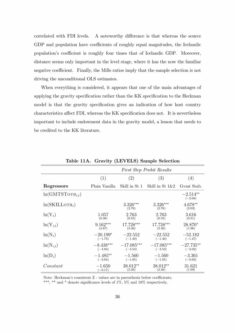
correlated with FDI levels. A noteworthy difference is that whereas the source

GDP and population have coefficients of roughly equal magnitudes, the Icelandic

population’s coefficient is roughly four times that of Icelandic GDP. Moreover,

distance seems only important in the level stage, where it has the now the familiar

negative coefficient. Finally, the Mills ratios imply that the sample selection is not

driving the unconditional OLS estimates.

When everything is considered, it appears that one of the main advantages of

applying the gravity specification rather than the KK specification to the Heckman

model is that the gravity specification gives an indication of how host country

characteristics affect FDI, whereas the KK specification does not. It is nevertheless

important to include endowment data in the gravity model, a lesson that needs to

be credited to the KK literature.

Table 11A. Gravity (LEVELS) Sample Selection


(1) (2) (3) (4)

Regressors Plain Vanilla Skill in St 1 Skill in St 1&2 Gvmt Stab.

ln(GMTSTothi,t) −2.514∗∗(−2.08)

ln(SKILLothi) 3.326∗∗∗(2.76)

3.326∗∗∗(2.76)

4.678∗∗(2.03)

ln(Yt) 1.057(0.30)

2.763(0.55)

2.763(0.55)

3.616(0.51)

ln(Yi,t) 9.162∗∗∗(4.87)

17.728∗∗∗(3.40)

17.728∗∗∗(3.40)

28.870∗(1.96)

ln(Nt) −20.199∗(−1.73)

−22.552(−1.40)

−22.552(−1.40)

−52.182(−1.47)

ln(Ni,t) −8.438∗∗∗(−4.94)

−17.085∗∗∗(−3.53)

−17.085∗∗∗(−3.53)

−27.735∗∗(−2.02)

ln(Di) −1.485∗∗(−2.04)

−1.560(−1.05)

−1.560(−1.05)

−3.361(−0.93)

Constant −1.650(−0.17)

38.012∗∗(2.26)

38.012∗∗(2.26)

31.621(1.09)


36

Table 11B. Gravity (LEVELS) Sample Selection


Regressors (1) (2) (3) (4)

ln(SKILLothi) 1.183(1.64)

0.628(0.75)

ln(Yt) 6.525(0.44)

7.353∗∗∗(2.98)

7.674∗∗∗(3.02)

7.309∗∗(2.23)

ln(Yi,t) −9.577(−0.28)

9.905∗∗∗(4.80)

12.215∗∗∗(5.06)

9.424∗∗∗(5.48)

ln(Nt) −7.816(−0.12)

−30.955∗∗∗(−4.33)

−31.291∗∗∗(−4.24)

−29.559∗∗∗(−4.08)

ln(Ni,t) 10.017(0.32)

−8.184∗∗∗(−4.34)

−10.583∗∗∗(−4.55)

−7.967∗∗∗(−4.78)

ln(Di) −3.529(−0.70)

−5.509∗∗∗(−8.65)

−5.048∗∗∗(−7.30)

−4.745∗∗∗(−4.26)

Constant −24.912(−0.45)

−5.794(−0.68)

7.467(0.59)

0.318(0.02)

Mills Ratio (λ) −4.319(−0.58)

0.189(0.33)

0.638(1.12)

0.013(0.03)

Observations 185 159 159 107

Uncens. Obs. 36 36 36 27


37

8.4 SHARES Heckman for the GRAVITY model

The final regression results presented in this paper include the Heckman procedure

applied to a gravity specification on FDI share data. These are presented in Tables

12A and 12B.

Like in the case of the KK model in Tables 9A and 10A, the estimates for the

first step in gravity level and gravity share data are fully identical. This is due to

the fact that both represent the likelihood of investment taking place in sector one

in general. However estimates obtained for the second step for share in Table 12B,

differ considerably from those in 11B.

Table 12A. Gravity (SHARES) Sample Selection


(1) (2) (3) (4)

Regressors Plain Vanilla Skill in St 1 Skill in St 1&2 Gvmt Stab.

ln(GMTSTothi,t) −2.514∗∗(−2.08)

ln(SKILLothi) 3.326∗∗∗(2.76)

3.326∗∗∗(2.76)

4.678∗∗(2.03)

ln(Yt) 1.057(0.30)

2.763(0.55)

2.763(0.55)

3.616(0.51)

ln(Yi,t) 9.162∗∗∗(4.87)

17.728∗∗∗(3.40)

17.728∗∗∗(3.40)

28.870∗(1.96)

ln(Nt) −20.199∗(−1.73)

−22.552(−1.40)

−22.552(−1.40)

−52.182(−1.47)

ln(Ni,t) −8.438∗∗∗(−4.94)

−17.085∗∗∗(−3.53)

−17.085∗∗∗(−3.53)

−27.735∗∗(−2.02)

ln(Di) −1.485∗∗(−2.04)

−1.560(−1.05)

−1.560(−1.05)

−3.361(−0.93)

Constant −1.650(−0.17)

38.012∗∗(2.26)

38.012∗∗(2.26)

31.621(1.09)


First, it is obvious that although the gravity model variables might help to

describe levels of FDI in sector one, they do little to describe the share of FDI in

that sector. They do indicate that as the Icelandic GDP grows, FDI is diversified

away from sector one. Estimates for distance indicate that once countries overcome

the threshold of investing in the power intensive sector, they are more likely to be

38

attracted to sector one than other sectors, with an increase in costs associated with

increased distance.

These last results give a nice end to the story, since the power intensive goods

are normally shipped and likely to be less distance sensitive than many other prod-

ucts. They might therefore become an increasingly preferable investment option,

compared to other investment opportunities, as distance increases.

All considered, it appears as if anything, the gravity model does marginally bet-

ter than the knowledge-capital approach, since the estimates obtained are slightly

more significant than those of the knowledge-capital model.

From Table 12B it can be concluded that a 1% increase in the source country

level of skill31 can be expected to result in about 0.2% increase in sector one share

of total FDI. Economically, this corresponds to the situation where if the source

country skilled labor (average of 21.35%) would move up by 1% i.e. to 21.56%,

then the share of sector one would increase from being 94.14% on average, to being

94.33% (note that the observations in the second step include only the years of

investment in sector one, and therefore the mean is very high).

Moreover, estimates indicate that as GDP in Iceland increases by 1%, then the

share of sector one in FDI decreases on by about 0.6%. The economic significance

of these estimates could be interpreted such that a 1% increase in Iceland GDP

from $7 billion32 to $7.07 billion would affect FDI such that the share of sector one

would go down from 94.14% to 93.67%.

As for source country GDP and population, as well as the population of Iceland,

coefficient estimates indicate that these economic factors would not effect the share

of sector one in overall FDI.

31These data are obtained from the International Labor Organization (ILO) as the sum ofoccupational categories 0/1 and 2; where category 0/1 accounts for professional, technical, andkindred workers, and category 2 for administrative workers. Moreover, the skilled labor ratio iscalculated as the sum of categories 0/1 and 2, divided by the sum of all occupational categories.The skilled labor ratio is used as a proxy for relative skilled labor abundance.32GDP values are on an 1995 base.

39

Table 12B. Gravity (SHARES) Sample Selection


Regressors (1) (2) (3) (4)

ln(SKILLothi) 0.208∗(1.73)

0.112(1.35)

ln(Yt) −0.563∗∗∗(−2.54)

−0.617∗∗∗(−2.77)

−0.561(−1.32)

−0.722∗∗(−2.15)

ln(Yi,t) 0.066(0.13)

−0.026(−0.14)

0.381(0.95)

0.053(0.29)

ln(Nt) 0.073(0.08)

0.424(0.65)

0.364(0.30)

0.287(0.38)

ln(Ni,t) −0.215(−0.46)

−0.129(−0.78)

−0.552(−1.43)

−0.234(−1.34)

ln(Di) 0.357∗∗∗(4.70)

0.366∗∗∗(6.39)

0.447∗∗∗(3.88)

0.444∗∗∗(4.05)

Constant −0.092(−0.11)

−0.108(−0.14)

2.229(1.06)

0.130(0.07)

Mills Ratio (λ) 0.043(0.38)

0.031(0.62)

0.110(1.17)

0.061(1.24)

Observations 185 159 159 107

Uncens. Obs. 36 36 36 27


Finally, estimates for distance indicate that an average increase in distance of

1% would involve an average increase in the share of sector one by about 0.4%.

The economic relationship effects of these changes could be interpreted such that

if distance would increase from its average by 1%, moving up from and average of

4000 kilometers to 4040 kilometers, then the share of sector one is estimated to go

up from 94.14% to 94.52%.

40

9 Conclusion

This paper presents analysis of foreign direct investment (FDI) allocated to different

investment sectors in Iceland. Both levels of FDI and shares of FDI are estimated.

When estimated separately, it appears that different forces are driving investment

in individual sectors. These results may possibly explain why the Knowledge Cap-

ital (KK) model specification of Carr, Markusen, Maskus (CMM) did not perform

particularly well for aggregate Icelandic data in my earlier paper (Kristjánsdóttir,

2004c). In order to take a closer look at the dominating investment sector in Ice-

land, the power intensive sector, the sector is analyzed specifically by applying the

Heckman two-step procedure to test for sample selection. Estimates indicate the

threshold of overcoming fixed cost does seem to be a critical issue when multina-

tionals choose to invest.

When sample selection is analyzed with a set of KK model variables, the proxy

for skill difference endowments is estimated to be negative for FDI levels, but pos-

itive in step two for FDI shares. This may indicate that source countries are

attracted by the level of skill in Iceland at the beginning stage of operations when

faced with fixed threshold cost. Once the plants have overcome fixed costs, there

are positive impacts on marginal investment the more skilled the source country is

compared to the host. The KK model estimates by the Heckman procedure indi-

cate that it appears as if the KK model analysis helps in explaining why countries

are likely to overcome fixed cost. Finally, when a set of gravity model variables are

applied in the Heckman procedure, it appears that they do a better job in explaining

the incentives for FDI. Estimates for endowments such as the level of skill of the

other country becomes more clear in the case of the gravity model, indicating that

an increase in the level of skill in the source country tends to positively effect both

on the investment undertaken initially and the marginal increase thereafter. Also,

source and host country market sizes have a clearer interpretation in the gravity

model case, especially the host country estimates. It therefore appears that the

gravity model does a better job explaining investment.

41

10 Appendix A. The Sample Selection Proce-dure

The sample selection procedure can be described as follows. I start by presenting the

equation determining sample selection equation (Greene, 1997, pp. 978) as Equation (5):

z∗i= γ0wi+ui, (4)

Following this I can present the basic model specification as shown in Eq. (6):

yi= β0xi+ i. (5)

Most of the time, the selection variable z∗ is not observed, but only its sign. In our

example, I observe only whether a source country invests in Iceland in a particular year

or not. This information implies the sign of z∗, but not its magnitude. Because I do

not have information on the scale of z∗, it is impossible to estimate the selection equation

variance.

Then the selection mechanism, capturing whether investment takes place or not, can

be put forward as shown in Eq. (7), where Prob refers to probability.:

z∗i = γ0wi + ui, z∗i = 1 if z∗i > 0 and 0 otherwise; (6)

Prob(zi = 1) = Φ(γ0wi) and

Prob(zi = 0) = 1− Φ(γ0wi).

The regression equation can be presented as follows:

yi = β0xi + i observed only if z∗i = 1, (7)

(ui, i) ∼ bivariate normal[0, 0, 1, σ , ρ].

If I then suppose that zi and wi are observed for a random sample of observations,

and that I only observe yi when zi=1, then I can present the model as follows:

(E[yi| zi= 1] = β0x+ ρσ λ(γ0w). (8)

42

11 Appendix B. The Kyoto Protocol

Kyoto Protocol to the United Nations framework convention on climate change33.

Third session Kyoto, 1-10 December 199734.

Quantified emission limitation or reduction commitment

(percentage of base year or period)

Australia 108% Liechtenstein 92%Austria 92% Lithuania* 92%Belgium 92% Luxembourg 92%Bulgaria* 92% Monaco 92%Canada 94% Netherlands 92%Croatia* 95% New Zealand 100%Czech Republic* 92% Norway 101%Denmark 92% Poland* 94%Estonia* 92% Portugal 92%European Community 92% Romania* 92%Finland 92% Russian Federation* 100%France 92% Slovakia* 92%Germany 92% Slovenia* 92%Greece 92% Spain 92%Hungary* 94% Sweden 92%Iceland 110% Switzerland 92%Ireland 92% Ukraine* 100%Italy 92% United Kingdom of Great BritainJapan 94% and Northern Ireland 92%Latvia* 92% United States of America 93%

* Countries that are undergoing the process of transition to a market economy

33English conference of the parties.34Source: www.cnn.com/SPECIALS/1997/global.warming/stories/treaty/index4.html

43

References

[1] Act on Investment (1996). Act on Investment by Non-residents in Business

Enterprises, No. 34 of 25 March 1991, as amended by Act No. 121 of 27 Decem-

ber 1993 and Act No. 46 of 22 May 1996. Based on the Icelandic Government

Gazette.

[2] Alfaro, L., A. Chandra, S. Kalemli-Ozcan and S. Sayek (2001) ”FDI and

Economic Growth: The Role of Local Financial Markets?” Harvard Business

School Working Paper 01-083.

[3] Anderson, J.E. (1979) A Theoretical Foundation for the Gravity Equation.

American Economic Review 69, p.106-116.

[4] Bergstrand, J.H. (1985), The Gravity Equation in International Trade: Some

microeconomic Foundations and Empirical Evidence, The Review of Economics

and Statistics, 67, p.474-481.

[5] Blonigen, B. A. and Davies, R. B. (2001). ”The Effects of Bilateral Tax Treaties

on U.S. FDI Activity”. University of Oregon Economics Department Working

Papers 2001-14, University of Oregon Economics Department.

[6] Blonigen, B. A., Davies, R. B. (2002). ”Asymmetric FDI and Tax-Treaty Bar-

gaining: Theory and Evidence,” Royal Economic Society Annual Conference

2002 48, Royal Economic Society.

[7] Blonigen, B. A. and Davies, R. B. (2003) ”Do Bilateral Tax Treaties Promote

FDI?” Handbook of International Trade and Law, forthcoming.

[8] Blonigen, B. A., Davies, R. B. and Head K. (2003). ”Estimating the

Knowledge-Capital Model of the Multinational Enterprise: Comment. Amer-

ican Economic Review, 93(3), pp. 980-94.

44

[9] Braconier, H., Norbäck P-J., and Urban D. (2002). ”Vertical FDI revisited”,

Working Paper No. 579, The Research Institute of Industrial Organization

(IUI). Stockholm, Sweden.

[10] Brainard, S. L. (1997). ”An Empirical Assessment of the Proximity-

Concentration Trade-off Between Multinational Sales and Trade,” American

Economic Review, 87(4): 520-44.

[11] Carr, D. L., Markusen, J. R. and Maskus, K. E. (2001). ”Estimating the

Knowledge-Capital Model of the Multinational Enterprise. American Eco-

nomic Review, 91(3): 693-708.

[12] Carr, D. L., Markusen, J. R. and Maskus, K. E. (2003). ”Estimating the

Knowledge-Capital Model of the Multinational Enterprise: Reply. American

Economic Review, 93(3), pp. 995-1001.

[13] Central Bank of Iceland (2001). Downloaded from<www.sedlabanki.is> Sept.

30th.

[14] Central Bank of Iceland (2001). Unpublished data on foreign direct investment

(FDI).

[15] Davies R., (2002). ”Hunting High and Low for Vertical FDI”, forthcoming.

[16] Devereux, M. B. and Lane P. R. (2002). ”Understanding Bilateral Exchange

Rate Volatility”. CEPR discussion paper No. 3518

[17] Distance Calculator (2000). How far is it. Downloaded from

<www.indo.com/distance/ index.html> June 11th.

[18] Economic Institute of Iceland (2000). Downloaded from

<www.Ths.is/hagvisar> May 10th.

[19] Czisch G., Lehner B. and Vassolo S. (2004) Downloaded from

<http://www.usf.uni-kassel.de /usf/archiv/ dokumente /kwws/5/ew_8_

hydropower_low.pdf> March 10th.

45

http://www.usf.uni-kassel.de

[20] Federal Reserve Bank of Cleveland (2003). Downloaded from

<www.clev.frb.org/research/Et99/1199/Html/Charts/Intdev1b.gif> Au-

gust 14th.

[21] Greene, W.H. (1997). Econometric Analysis. Prentice Hall, New Jersey.

[22] Grosse R. (1997). ”Foreign Direct Investment in Latin America”. In Robert

Grosse, ed., Generating Savings for Latin American Development, Boulder CO:

Lynne Rienner Publishers pp. 135

[23] Gylfason, Th. (2000). Að opna lönd. Vísbending. 18(50): 2-3.

[24] Gylfason, Th. and G. Zoega (2001). Natural Resources and Economic Growth:

The Role of Investment. CEPR Discussion Paper No. 2743.

[25] Heckman, J. (1979). ”Sample selection bias as a specification error”. Econo-

metrica, 47, pp. 153-161.

[26] Helpman, E. (1984). ”A Simple Theory of Interna tional Trade with Multina-

tional Corporations.” Journal of Political Economy, 92(31): 451-71.

[27] Helpman, E. (1987). ”Imperfect Competition and International Trade: Evi-

dence from Fourteen Industrial Countries”, Journal of the Japanese and Inter-

national Economies 1: 62-81.

[28] Helpman, E. (1998). ”The Structure of Foreign Trade”. Working Paper No.

6752. NBER Working Paper Series. National Bureau of Economic Research.

[29] Helpman, E. (1999). ”The Structure of Foreign Trade”, Journal of Economic

Perspectives, 13(2): 121-144.

[30] Helpman, E. and Krugman, P. (1985). Market structure and foreign trade,

Cambridge, MA: MIT Press.

[31] International Monetary Fund (2000). Balance of Payments Manual, (5th edi-

tion) (BPM5).

46

[32] Jeon, B.N. and Stone, S.F. (1999). ”Gravity-Model Specification for Foreign

Direct Investment: A case of the Asia-Pacific Economies”, The Journal of

Business and Economic Studies. 5(1), Fairfield University.

[33] Ju-e, G. (2000). ”Some Trends on Change in Direct Input Co-

efficient of China”. Paper for the Thirteenth International Confer-

ence on Input-Output Techniques, Macerata, Italy. Downloaded from

<www.http://policy.rutgers.edu/cupr/iioa/Guo-DirectCoeffs.pdf>April 15th,

2004.

[34] Kristinsson, T.Ö. (1996). ”Bjartsýni á álmörkuðum”, Vísbending, 14(41).

[35] Kristjánsdóttir, H. (2004a) ”A Gravity Model for Exports from Iceland”. The-

sis paper. University of Iceland, Reykjavík, Iceland.

[36] Kristjánsdóttir, H. (2004b) ”Determinants of Foreign Direct Investment in

Iceland”. Thesis paper. University of Iceland, Reykjavík, Iceland.

[37] Kristjánsdóttir, H. (2004c) ”The Knowledge-Capital Model and Small Coun-

tries”. Thesis paper. University of Iceland, Reykjavík, Iceland.

[38] Kyoto Protocal to the United Nations framework convention on climate

change (1997). Third session Kyoto, 1-10 December. Downloaded from

<www.cnn.com/SPECIALS/1997/global.warming/stories/treaty/index4.html>

May 10th, 2002.

[39] Markusen, J.R. (1984). ”Multinationals, Multi-plant Economies, and the

Gains from Trade.”. Journal of International Economics, 16(3-4): 205-26.

[40] Markusen, J. R. (1998). ”Multinational Enterprises and the Theories of Trade

and Location”. In P. Braunerhjelm and K. Ekholm, eds., The Geography of

Multinational Firms, Boston, Kluwer Academic Publishers, pp.10-14.

[41] Markusen, J. R. andMaskus K. E. (2001). ”Multinational Firms: Reconcililing

Theory and Evidence”. In M. Blomstrom and L. S. Goldberg, eds., Topics in

47

http://policy.rutgers.edu/cupr/iioa/Guo-DirectCoeffs.pdf

Empirical International Economics: A Festschrift in Honor of Robert E. Lipsey.

Chicago, IL: University of Chicago Press for National Bureau of Economic

Research.

[42] Markusen, J. R. and Maskus K. E. (2002). ”Discriminating among Alternative

Theories of the Multinational Enterprise”, Review of International Economics,

10(4), 694-707.

[43] Razin A., Rubinstein Y. and E. Sadka (2003). ”Which Countries Export FDI,

and How Much?”. Paper presented at the 6th Conference of the Analysis

of International Capital Markets RTN, hosted By: Universita di Roma III,

December 2003. Downloaded from <www.cepr.org> March 30th, 2004, pp.

2-4.

[44] Slaughter, M. J. (2000). ”Production Transfer Within Multinational Enter-

prises and American Wages.” Journal of International Economics, 50(2), pp.

449-472

[45] Smits J. (2003). ”Estimating the Heckman two-step procedure to control

for selection bias with SPSS”. Downloaded from <http://home.planet.nl/

~smits.jeroen> March 30th, 2004, pp. 4

[46] Wagner W. (1998). ”Aluminum”. Natural Resources Canada. Downloded

from http://www.nrcan-rncan.gc.ca/ mms/cmy/content/1998/09.pdf

[47] Waldkirch A. (2002). ”Vertical FDI? A Host Country Perspective.” Review of

International Economics, 10(4), 694-707.

[48] Verbeek, M. (2000). A Guide to Modern Econometrics, John Wiley and Sons.

[49] World Bank (2002). World Development Indicators. CD-Rom.

[50] World Competitiveness Report (1989-1995).

[51] World Competitiveness Yearbook (1996-2000).

48

http://home.planet.nl/

http://www.nrcan-rncan.gc.ca/

EPRU Working Paper Series - CORE

Documents

Transcript of EPRU Working Paper Series - CORE