Multiscale methods for shape constraints in deconvolution: Confidence statements for qualitative...

Multiscale Methods for Shape

Constraints in Deconvolution:

Confidence Statements for Qualitative

Features

Johannes Schmidt-Hieber Axel Munk and Lutz Dumbgen

Department of MathematicsVrije Universiteit Amsterdam

De Boelelaan 1081a,1081 HV Amsterdam

Netherlandse-mail: [email protected]

Institut fur Mathematische StochastikUniversitat Gottingen

Goldschmidtstr. 7D-37077 Gottingen

andMax-Planck Institute

for Biophysical ChemistryAm Fassberg 11

D-37077 GottingenGermany

e-mail: [email protected]

Institut fur mathematische Stochastikund Versicherungslehre

Universitat BernAlpeneggstrasse 22

CH-3012 BernSwitzerland

e-mail: [email protected]

Abstract: We derive multiscale statistics for deconvolution in order todetect qualitative features of the unknown density. An important examplecovered within this framework is to test for local monotonicity on all scalessimultaneously. We investigate the moderately ill-posed setting, where theFourier transform of the error density in the deconvolution model is ofpolynomial decay. For multiscale testing, we consider a calibration, moti-vated by the modulus of continuity of Brownian motion. We investigatethe performance of our results from both the theoretical and simulationbased point of view. A major consequence of our work is that the detectionof qualitative features of a density in a deconvolution problem is a doabletask although the minimax rates for pointwise estimation are very slow.

AMS 2000 subject classifications: Primary 62G10; secondary 62G15,62G20.Keywords and phrases: Brownian motion, convexity, pseudo-differentialoperators, ill-posed problems, mode detection, monotonicity, multiscale statis-tics, shape constraints.

1

arX

iv:1

107.

1404

v3 [

mat

h.ST

] 1

7 D

ec 2

012

mailto:[email protected]



J. Schmidt-Hieber et al./Confidence Statements for Qualitative Features 2

1. Introduction

We observe Y = (Y1, . . . , Yn) according to the deconvolution model

Yi = Xi + εi, i = 1, . . . , n, (1)

whereXi, εi, i = 1, . . . , n are assumed to be real valued and independent,Xii.i.d.∼

X, εii.i.d.∼ ε and Y1, X, ε have densities g, f and fε, respectively. Our goal is to

develop multiscale test statistics for certain structural properties of f , wherethe density fε of the blurring distribution is assumed to be known.

Although estimation in deconvolution models has attracted a lot of attentionduring the last decades (cf. Fan [17], Diggle and Hall [12], Pensky and Vi-dakovic [41], Johnstone et al. [29], Butucea and Tsybakov [7] as well as Meister[38] for some selective references), inference about f and its qualitative featuresis rather less well studied. In fact, adaptive confidence bands would be desirablebut turn out to be very ambitious. First, they suffer from the bad convergencerates induced by the ill-posedness of the problem (cf. Bissantz et al. [5]), mak-ing confidence bands less attractive for applications. Second, one would needto circumvent the classical problems of honest adaptation over Holder scales.To overcome these difficulties the aim of the paper is to derive simultaneousconfidence statements for qualitative features of f.

Structural properties or shape constraints will be conveniently expressed as(pseudo)-differential inequalities of the density f , assuming for the moment thatf is sufficiently smooth. Important examples are f ′ ≷ 0 to check local mono-tonicity properties as well as f ′′ ≷ 0 for local convexity or concavity. To giveanother example, suppose that we are interested in local monotonicity propertiesof the density f of exp(aX) for given a > 0. Since f(s) = (as)−1f(a−1 log(s)),one can easily verify that local monotonicity properties of f may be expressedin terms of the inequalities f ′ − af ≶ 0.

This paper deals with the moderately ill-posed case, meaning that the Fouriertransform of the blurring density fε decays at polynomial rate. In fact, we workunder the well-known assumption of Fan [17] (cf. Assumption 2), which essen-tially assures that the inversion operator, mapping g 7→ f , is pseudo-differential.This combines nicely with the assumption on the class of shape constraints. Ourframework includes many important error distributions such as Exponential, χ2,Laplace and Gamma distributed random variables. The special case ε = 0 (i.e.no deconvolution or direct problem) can be treated as well, of course.

1.1. Example: Detecting trends in deconvolution

To illustrate the key ideas, suppose that we are interested in detection of regionsof increase and decrease of the true density in Laplace deconvolution, that is,the error density is given by fε = (2θ)−1 exp(−| · |/θ). Let φ be a sufficientlysmooth, non-negative kernel function (i.e.

∫φ(u)du = 1), supported on [0, 1].


Then, since f = g − θ2g′′ in this case, it follows by partial integration that

Tt,h :=1

h√n

n∑k=1

(θ2

h2φ(3)

(Yk − th

)− φ′

(Yk − th

)). (2)

has expectation ETt,h =√n∫ t+ht

φ( s−th)f ′(s)ds. The construction of the multi-

scale test relies on the following analytic observation. Suppose that for a givenpair (t, h) there is a number dt,h such that

|Tt,h − ETt,h| ≤ dt,h. (3)

If in addition Tt,h > dt,h, then necessarily

ETt,h =√n

∫ t+h

t

φ(s−th

)f ′(s)ds > 0 (4)

and by the non-negativity of φ, f(s1) < f(s2) for some points s1 < s2 in[t, t + h]. On the contrary, Tt,h < −dt,h implies that there is a decrease on[t, t+ h]. For a sequence Nn = o(n/ log3 n) tending to infinity faster than log3 nand un = 1/ log logn, define

Bn :={( k

Nn,l

Nn

) ∣∣ k = 0, 1, . . . , l = 1, 2, . . . , [Nnun], k + l ≤ Nn}.

Given α ∈ (0, 1), we will be able to compute bounds dt,h such that for all(t, h) ∈ Bn, inequality (3) holds simultaneously with asymptotic probability1 − α. Taking into account that (3) implies (4), this allows to identify regionsof increase and decrease for prescribed probability.

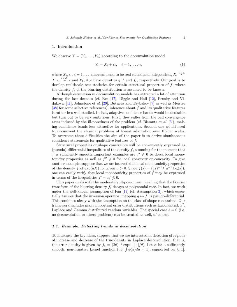
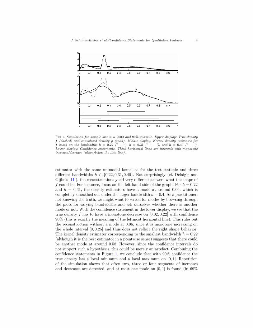
Figure 1 shows a simulation result for n = 2000, Nn = bn3/5c, θ = 0.075 andconfidence level 90%. The upper panel of Figure 1 displays the true density of fas well as the convoluted density g. Notice that we only have observations withdensity g. In fact, by visual inspection of g it becomes apparent how difficult itis to find segments on which f is monotone increasing/decreasing.

The lower panel of Figure 1 displays intervals for which we can concludethat there is a monotone increase/decrease. Let us give precise instructions onhow to read this plot: Pick any of the thick horizontal lines. Then, with overallprobability 90%, somewhere in this interval there is a monotone increase ordecrease of f , depending on whether it is drawn above or below the thin line,respectively. In particular, the fact that intervals with monotone increase anddecrease overlap does not yield a contradiction, since the statement is that themonotonicity holds only on a non-empty subset of the corresponding interval.(The way the intervals are piled up in the plot, besides the fact that they areabove or below the thin line, is arbitrary and does not contain information.)Recall that we have uniformity in the sense that with confidence 90% all thesestatements are true simultaneously (cf. also Dumbgen and Walther [14]).

To illustrate our approach consider the middle panel in Figure 1. Here, wehave displayed three reconstructions using t 7→ Tt,h/(h

√n) as kernel density


Fig 1. Simulation for sample size n = 2000 and 90%-quantile. Upper display: True densityf (dashed) and convoluted density g (solid). Middle display: Kernel density estimates forf based on the bandwidths h = 0.22 (’ ’), h = 0.31 (’ ’), and h = 0.40 (’ ’).Lower display: Confidence statements. Thick horizontal lines are intervals with monotoneincrease/decrease (above/below the thin line).

estimator with the same unimodal kernel as for the test statistic and threedifferent bandwidths h ∈ {0.22, 0.31, 0.40}. Not surprisingly (cf. Delaigle andGijbels [11]), the reconstructions yield very different answers what the shape off could be. For instance, focus on the left hand side of the graph. For h = 0.22and h = 0.31, the density estimators have a mode at around 0.06, which iscompletely smoothed out under the larger bandwidth h = 0.4. As a practitioner,not knowing the truth, we might want to screen for modes by browsing throughthe plots for varying bandwidths and ask ourselves whether there is anothermode or not. With the confidence statement in the lower display, we see that thetrue density f has to have a monotone decrease on [0.02, 0.22] with confidence90% (this is exactly the meaning of the leftmost horizontal line). This rules outthe reconstruction without a mode at 0.06, since it is monotone increasing onthe whole interval [0, 0.25] and thus does not reflect the right shape behavior.The kernel density estimator corresponding to the smallest bandwidth h = 0.22(although it is the best estimator in a pointwise sense) suggests that there couldbe another mode at around 0.58. However, since the confidence intervals donot support such a hypothesis, this could be merely an artefact. Combining theconfidence statements in Figure 1, we conclude that with 90% confidence thetrue density has a local minimum and a local maximum on [0, 1]. Repetitionof the simulation shows that often two, three or four segments of increasesand decreases are detected, and at most one mode on [0, 1] is found (in 69%


of the cases). Therefore, sample size n = 2000 is not large enough to detectsystematically the correct number of minima and maxima (2 and 3). Numericalsimulations for larger sample size and more details are given in Section 6.

The derived confidence statements should be viewed as an additional toolfor analyzing data, in particular for substantiating vague conclusions or visualimpressions from point estimators.

1.2. Pseudo-differential operators and multiscale analysis

As mentioned at the beginning of the introduction, we interpret shape con-straints as pseudo-differential inequalities. Let F(f) =

∫R exp (−ix·) f(x)dx al-

ways denote the Fourier transform of f ∈ L1 (R) or f ∈ L2 (R) (depending onthe context). Consider a general class of differential operators op(p) with symbolp which can be written for nice f as

(op(p)f)(x) =1

2π

∫eixξp(x, ξ)F(f)(ξ)dξ. (5)

This class will be an enlargement of (elliptic) pseudo-differential operators byfractional differentiation. Given data from model (1) the goal is then to identifyintervals at a controlled error level on which Re(op(p)f) 6≤ 0 or Re(op(p)f) 6≥ 0.Here Re denotes the projection on the real part. In Subsection 1.1 we studiedimplicitly already the case of op(p) being the differentiation operator Df = f ′

(monotonicity). If applied to op(p) = D2 (i.e. p(x, ξ) = −ξ2), our method yieldsbounds for the number and confidence regions for the location of inflectionpoints of f . We also discuss an example related to Wicksell’s problem withshape constraint described by fractional differentiation.

The statistic introduced in this paper investigates shape constraints of the un-known density f on all scales simultaneously. Generalizing (4), we need to derivesimultaneous confidence intervals for 〈φ ◦ St,h,Re(op(p)f)〉 with the scale-and-location shift St,h = (·−t)/h and the inner product 〈h1, h2〉 :=

∫R h1(x)h2(x) dx

in L2. If op(p)? is the adjoint of op(p) (in a certain space) with respect to 〈·, ·〉,then

√n⟨φ ◦ St,h,Re op(p)f

⟩=√n Re

∫ (op(p)?(φ ◦ St,h)

)(x)f(x)dx

=

√n

2πRe

∫F(

op(p)?(φ ◦ St,h))(s)F(f)(s)ds (6)

and the r.h.s. can be estimated unbiasedly by the test statistic

Tt,h := n−1/2n∑k=1

Re vt,h(Yk)

with

vt,h(u) :=1

2π

∫F(

op(p)?(φ ◦ St,h))(s)

eisu

F(fε)(−s)ds.


This gives rise to a multiscale statistic

Tn = sup(t,h)

wh

(∣∣Tt,h − ETt,h∣∣

Std(Tt,h)− wh

),

where wh and wh are chosen in order to calibrate the different scales with equal

weight, while Std(Tt,h) is an estimator of the standard deviation of Tt,h.The key result in this paper is the approximation of Tn by a distribution-free

statistic from which critical values can be inferred. Given the critical values, wecan in a second step compute bounds dt,h such that a statement of type (3) holds.Following the same ideas as in Subsection 1.1, this is enough to identify intervalson which Re(op(p)f) 6≤ 0 or Re(op(p)f) 6≥ 0. In fact the multiscale methodimplies confidence statements which are stronger than the ones described up tonow. These objects can be related to superpositions of confidence bands. Formore precise statements see Section 4.

1.3. Comparison with related work and applications

Hypothesis testing for deconvolution and related inverse problems is a relativelynew area. Current methods cover testing of parametric assumptions (cf. [4, 34,6]) and, more recently, testing for certain smoothness classes such as Sobolevballs in a Gaussian sequence model (Laurent et al. [35, 34] and Ingster et al.[28]). All these papers focus on regression deconvolution models. Exceptionsfor density deconvolution are Holzmann et al. [25], Balabdaoui et al. [3], andMeister [39] who developed tests for various global hypotheses, such as globalmonotonicity. The latter test has been derived for one fixed interval and allowsto check whether a density is monotone on that interval at a preassigned levelof significance.

Our work can also be viewed as an extension of Chaudhuri and Marron [8]as well as Dumbgen and Walther [14] who treated the case op(p) = Dm (withm = 1 in [14]) in the direct case, i.e. when ε = 0. However, the approachin [8] does not allow for sequences of bandwidths tending to zero and yieldslimit distributions depending on unknown quantities again. The methods in[14] require a deterministic coupling result. The latter allows to consider themultiscale approximation for f = I[0,1] only, but it cannot be transferred to thedeconvolution setting.

One of the main advantages of multiscale methods, making it attractive forapplications, is that essentially no smoothing parameter is required. The mainchoice will be the quantile of the multiscale statistic, which has a clear proba-bilistic interpretation. Furthermore, our multiscale statistic allows to constructestimators for the number of modes and inflection points which have a num-ber of nice properties: First, modes and inflection points are detected with theminimax rate of convergence (up to a log-factor). Second, the probability thatthe true number is overestimated can be made small, since it is completelycontrolled by the quantile of the multiscale statistic. To state it differently, it


is highly unlikely that artefacts are detected, which is a desirable property inmany applications. It is worth noting that neither assumptions are made on thenumber of modes nor additional model selection penalties are necessary.

For practical applications, we may use these models if for instance the errorvariable ε is an independent waiting time. For example let Xi be the (unknown)time of infection of the i-th patient, εi the corresponding incubation time, and Yiis the time when diagnosis is made. Then, it is convenient to assume ε ∼ Γ (r, θ)(see for instance [10], Section 3.5). By the techniques developed in this paper onewill be able to identify for example time intervals where the number of infectionsincreased and decreased for a specified confidence level. Another applicationis single photon emission computed tomography (SPECT), where the detectedscattered photons are blurred by Laplace distributed random variables (cf. Floydet al. [18], Kacperski et al. [30]).

The paper is organized as follows. In Section 2 we show how distribution-freeapproximations of multiscale statistics can be derived for general empirical pro-cesses under relatively weak conditions. For the precise statement see Theorem1. These results are transferred to shape constraints and deconvolution mod-els in Section 3. In Section 4 we discuss the statistical consequences and showhow confidence statements can be derived. Theoretical questions related to theperformance of the multiscale method and numerical aspects are discussed inSections 5 and 6. Proofs and further technicalities are shifted to the appendix.

Notation: We write T for the set [0, 1]× (0, 1]. The expression bxc means thelargest integer not exceeding x. The support of a function φ is suppφ, ‖ · ‖pdenotes the norm in Lp := Lp(R), and TV(·) stands for the total variationof functions on R. As customary in the theory of Sobolev spaces, put 〈s〉 :=(1 + |s|2)1/2. One should not confuse this with 〈·, ·〉, the L2-inner product. If itis clear from the context, we write xkφ and 〈x〉kφ for the functions x 7→ xkφ(x)and x 7→ 〈x〉kφ(x), respectively. The (L2-)Sobolev space Hr is defined as theclass of functions with norm

‖φ‖Hr :=(∫〈s〉2r|F(φ)(s)|2ds

)1/2<∞.

For any q and ` ∈ N (N is always the set of non-negative integers) define Hq` as

the Sobolev type space

Hq` :=

{ψ | xkψ ∈ Hq, for k = 0, 1, . . . , `

}with norm ‖ψ‖Hq` :=

∑`k=0 ‖xkψ‖Hq .

2. A general multiscale test statistic

In this section, we shall give a fairly general convergence result which is of inter-est on its own. The presented result does not use the deconvolution structure ofmodel (1). It only requires that we have observations Yi = G−1(Ui), i = 1, . . . , n


with Ui i.i.d. uniform on [0, 1] and G an unknown distribution function withLebesgue density g in the class

G := Gc,C,q :={G∣∣ G is a distribution function with density g,

c ≤ g∣∣[0,1]

, ‖g‖∞ ≤ c−1, and g ∈ J (C, q)}

(7)

for fixed c, C ≥ 0, 0 ≤ q < 1/2, and the Lipschitz type constraint

J := J (C, q)

:={h∣∣ |√h(x)−

√h(y)| ≤ C(1 + |x|+ |y|)q|x− y|, for all x, y ∈ R

}.

For a set of real-valued functions (ψt,h)t,h define the test statistic (empiricalprocess) Tt,h = n−1/2

∑nk=1 ψt,h(Yk). If h is small and ψt,h localized around t,

then Std(Tt,h) ≈ (∫ψ2t,h(s)g(s)ds)1/2 ≈ ‖ψt,h‖2

√g(t). It will turn out later on

that one should allow for a slightly regularized standardization and thereforewe consider

|Tt,h − E[Tt,h]|Vt,h

√gn(t)

with Vt,h ≥ ‖ψt,h‖2 and gn an estimator of g, satisfying

supG∈G‖gn − g‖∞ = OP (1/ log n). (8)

Unless stated otherwise, asymptotic statements refer to n → ∞. We combinethe single test statistics for an arbitrary subset

Bn ⊂{

(t, h)∣∣ t ∈ [0, 1], h ∈ [ln, un]

}(9)

and consider for ν > e and

wh =

√12 log ν

h

log log νh

, (10)

distribution-free approximations of the multiscale statistic

Tn := sup(t,h)∈Bn

wh

(∣∣Tt,h − E[Tt,h]∣∣

Vt,h√gn(t)

−√

2 log νh

). (11)

Assumption 1 (Assumption on test functions). Given a set Bn of the form(9), functions (ψt,h)(t,h)∈T , and numbers (Vt,h)(t,h)∈T , suppose that the followingassumptions hold.

(i) For all (t, h) ∈ T , ‖ψt,h‖2 ≤ Vt,h.(ii) We have uniform bounds on the norms

sup(t,h)∈T

√hTV(ψt,h) +

√h‖ψt,h‖∞ + h−1/2‖ψt,h‖1Vt,h

. 1.


(iii) There exists α > 1/2 such that

κn := sup(t,h)∈Bn, G∈G

whTV

(ψt,h(·)

[√g(·)−

√g(t)

]〈·〉α

)Vt,h

→ 0.

(iv) There exists a constant K such that for all (t, h), (t′, h′) ∈ T ,√h ∧√h′

Vt,h ∨ Vt′,h′

[‖ψt,h − ψt′,h′‖2 + |Vt,h − Vt′,h′ |

]≤ K

√|t− t′|+ |h− h′|.

Theorem 1. Given a multiscale statistic of the form (11). Work in model (1)under Assumption 1 and suppose that lnn log−3 n → ∞ and un = o(1). If theprocess (t, h) 7→

√hV −1t,h

∫ψt,h(s)dWs has continuous sample paths on T , then

there exists a (two-sided) standard Brownian motion W , such that for ν > e,

supG∈Gc,C,q

∣∣∣Tn − sup(t,h)∈Bn

wh

(∣∣ ∫ ψt,h(s)dWs

∣∣Vt,h

−√

2 log νh

)∣∣∣ = OP (rn), (12)

with

rn = supG∈G

∥∥gn − g∥∥∞ log n

log log n+ l−1/2n n−1/2

log3/2 n

log log n+

√un log(1/un)

log log(1/un)+ κn.

Moreover,

sup(t,h)∈T

wh


∣∣Vt,h

−√

2 log νh

)<∞, a.s. (13)

Hence, the approximating statistic in (12) is almost surely bounded from above.

The proof of the coupling in this theorem (cf. Appendix A) is based on gen-eralizing techniques developed by Gine et al. [19], while finiteness of the approx-imating test statistic utilizes results of Dumbgen and Spokoiny [13]. Note thatTheorem 1 can be understood as a multiscale analog of the L∞-loss convergencefor kernel estimators (cf. [20, 19, 5, 21]).

To give an example, let us assume that ψt,h = ψ( ·−th ) is a kernel function.

By Lemmas B.12 and B.4, Assumption 1 holds for Vt,h = ‖ψt,h‖2 =√h‖ψ‖2

whenever ψ 6= 0 on a Lebesgue measurable set, TV(ψ) < ∞ and suppψ ⊂[0, 1]. Furthermore, by partial integration, we can easily verify that the process(t, h) 7→ ‖ψ‖−12

∫ψt,h(s)dWs has continuous sample paths (cf. [13], p. 144).

For an application of Theorem 1 to wavelet thresholding, cf. Example 4 inthe appendix. Let us close this section with a result on the lower bound of theapproximating statistic.

Theorem 1 shows that the approximating statistic is almost surely boundedfrom above. On the contrary, we have the trivial lower bound

Tn ≥ − inf(t,h)∈Bn

log νh

log log νh

,


which converges to −∞ in general and describes the behavior of Tn, providedthe cardinality of Bn is small (for instance if Bn contains only one element).However, if Bn is sufficiently rich, Tn can be shown to be bounded from below,uniformly in n. Let us make this more precise. Assume, that for every n thereexists a Kn such that Kn →∞ and

B◦Kn :={(

iKn, 1Kn

) ∣∣ i = 0, . . . ,Kn − 1}⊂ Bn. (14)

Then, the approximating statistic is asymptotically bounded from below by−1/4. This follows from Lemma C.1 in the appendix. It is a challenging prob-lem to calculate the distribution for general index set Bn explicitly. Althoughthe tail behavior has been studied for the one-scale case (cf. [19, 5]) this has notbeen addressed so far for the approximating statistic in Theorem 1. For imple-mentation, later on, our method relies therefore on Monte Carlo simulations.

3. Testing for shape constraints in deconvolution

We start by defining the class of differential operators in (5). However, beforemaking this precise, let us define pseudo-differential operators in dimension oneas well as fractional integration and differentiation. Given a real m, consider Sm

the class of functions a : R× R→ C such that for all α, β ∈ N,

|∂βx∂αξ a(x, ξ)| ≤ Cα,β(1 + |ξ|)m−α for all x, ξ ∈ R. (15)

Then the pseudo-differential operator Op(a) corresponding to the symbol a canbe defined on the Schwartz space of rapidly decreasing functions S by

Op(a) : S → S

Op(a)φ(x) :=1

2π

∫eixξa(x, ξ)F(φ)(ξ)dξ.

It is well-known that for any s ∈ R, Op(a) can be extended to a continuousoperator Op(a) : Hm+s → Hs. In order to simplify the readability, we only writeOp for pseudo-differential operators and op in general for operators of the form(5). Throughout the paper, we write ιαs = exp(απi sign(s)/2) and understandas usual (±is)α = |s|αι±αs . The Gamma function evaluated at α will be denotedby Γ(α). Let us further introduce the Riemann-Liouville fractional integrationoperators on the real axis for α > 0 by

(Iα+h

)(x) :=

1

Γ(α)

∫ x

−∞

h(t)

(x− t)1−αdt and

(Iα−h

)(x) :=

1

Γ(α)

∫ ∞x

h(t)

(t− x)1−αdt. (16)

For β ≥ 0, we define the corresponding fractional differentiation operators(Dβ

+h)(x) := Dn(In−β+ h)(x) and (Dβ−h)(x) = (−D)n(In−β− f)(x), where n =


bβc+1. For any s ∈ R, we can extend Dβ+ and Dβ

− to continuous operators fromHβ+s → Hs using the identity (cf. [31], p.90),

F(Dβ±h)(ξ) = (±iξ)βF

(h)(ξ) = ι±βξ |ξ|

βF(h)(ξ). (17)

In this paper, we consider operators op(p) which “factorize” into a pseudo-differential operator and a fractional differentiation in Riemann-Liouville sense.More precisely, the symbol p is in the class

Sm :={

(x, ξ) 7→ p(x, ξ) = a(x, ξ)|ξ|γιµξ∣∣ a ∈ Sm, m = m+ γ,

γ ∈ {0} ∪ [1,∞), µ ∈ R}.

Let us mention that we cannot allow for all γ ≥ 0 since in our proofs it is essentialthat ∂2ξp(x, ξ) is integrable. The results can also be formulated for finite sums

of symbols, i.e.∑Jj=1 pj and pj ∈ Sm. However, for simplicity we restrict us to

J = 1.Throughout the remaining part of the paper, we will always assume that

op(p)f is continuous. A closed rectangle in R2 parallel to the coordinate axeswith vertices (a1, b1), (a1, b2), (a2, b1), (a2, b2), a1 < a2, b1 < b2 will be denotedby [a1, a2]× [b1, b2].

The main objective of this paper is to obtain uniform confidence statementof the following kinds:

(i) The number and location of the roots and maxima of op(p)f .(ii) Simultaneous identification of intervals of the form [ti, ti+hi], ti ∈ [0, 1], hi >

0, i in some index set I, with the following property: For a pre-specifiedconfidence level we can conclude that for all i ∈ I the functions (op(p)f)|[ti,ti+hi]attain, at least on a subset of [ti, ti + hi], positive values.

(ii′) Same as (ii), but we want to conclude that (op(p)f)|[ti,ti+hi] has to attainnegative values.

(iii) For any pair (t, h) ∈ Bn with Bn as in (9), we want to find b−(t, h, α) andb+(t, h, α), such that we can conclude that with overall confidence 1− α,the graph of op(p)f (denoted as graph(op(p)f) in the sequel) has a non-empty intersection with every rectangle [t, t+h]× [b−(t, h, α), b+(t, h, α)].

In the following we will refer to these goals as Problems (i), (ii), (ii′) and(iii), respectively. Note that (ii) follows from (iii) by taking all intervals [t, t+h]with b−(t, h, α) > 0. Analogously, [t, t+h] satisfies (ii′) whenever b+(t, h, α) < 0.The geometrical ordering of the intervals obtained by (ii) and (ii′) yields in astraightforward way a lower bound for the number of roots of op(p)f , solvingProblem (i) (cf. also Dumbgen and Walther [14]). A confidence interval for thelocation of a root can be constructed as follows: If there exists [t, t+h] such that

b−(t, h, α) > 0 and [t, t + h] with b+(t, h, α) < 0, then, with confidence 1 − α,

op(p)f has a zero in the interval[min(t, t),max(t + h, t + h)

]. The maximal

number of disjoint intervals on which we find zeros is then an estimator for thenumber of roots.


Example 1. In the example in Section 1.1 we had op(p) = D. In this case wewant to find a collection of intervals [t, t + h] such that with overall probability1 − α for each such interval there exists a nondegenerate subinterval on whichf is strictly monotonically increasing/decreasing.

Instead of studying qualitative features of X directly, we might as well beinterested in properties of the density of a transformed random variable q(X).If X is non-negative and a > 0, q could be for instance a (slightly regularized)log-transform q = log(·+ a).

Example 2. Suppose that we want to analyze the convexity/concavity propertiesof U = q(X), where q is a smooth function, which is strictly monotone increasingon the support of the distribution of X. Let fU denote the density of U . Then,by change of variables

fU (y) =1

q′(q−1(y)

)f(q−1(y)),

and there is a pseudo-differential operator Op(p) with symbol

p(x, ξ) = − 1

(q′(x))2ξ2 − q′′(x)q′(x) + 2q′′(x)

(q′(x))4iξ +

3(q′′(x))2 − q′′′(x)q′(x)

(q′(x))5,

such that f ′′U (y) = (op(p)f)(q−1(y)). Therefore,

graph(op(p)f) ∩ [t, t+ h]× [b−(t, h, α), b+(t, h, α)] 6= ∅

implies

graph(f ′′U ) ∩ [q(t), q(t+ h)]× [b−(t, h, α), b+(t, h, α)] 6= ∅.

In particular, if b−(t, h, α) > 0 then, with confidence 1 − α, we may concludethat fU is strictly convex on a nondegenerate subinterval of [q(t), q(t+ h)].

Example 3 (Noisy Wicksell problem). In the classical Wicksell problem, cross-sections of a plane with randomly distributed balls in three-dimensional space areobserved. From these observations the distribution H or density h = H ′ of thesquared radii of the balls has to be estimated (cf. Groeneboom and Jongbloed[23]). Statistically speaking, we have observations X1, . . . , Xn with density fsatisfying the following relationship (cf. Golubev and Levit [22])

1−H(x) ∝∫ ∞x

f(t)

(t− x)1/2dt = Γ( 1

2 )(I1/2− f)(x), for all x ∈ [0,∞),

where ∝ means up to a positive constant and I1/2− as in (16). Suppose now,

that we are interested in monotonicity properties of the density h = H ′ on[0, 1]. For x > 0, −h′ ≶ 0 iff the fractional derivative of order 3/2 satisfies

(D3/2− f)(x) = D2(I

1/2− f)(x) ≶ 0. It is reasonable to assume in applications that

the observations are corrupted by measurement errors, which means we onlyobserve Yi = Xi + εi as in model (1). Hence, we are in the framework described

above and the shape constraint is given by op(p)f ≶ 0 for p(x, ξ) = ι−3/2ξ |ξ|3/2.


In order to formulate our results in a proper way, let us introduce the follow-ing definitions. We say that a pseudo-differential operator Op(a) with a ∈ Smand Sm as in (15), is elliptic, if there exists ξ0 such that |a(x, ξ)| > K|ξ|mfor a positive constant K and all ξ satisfying |ξ| > |ξ0|. In the framework ofExample 2 for instance, ellipticity holds if ‖q′‖∞ < ∞. It is well-known thatellipticity is equivalent to a generalized invertibility of the operator. Further-more, for an arbitrary symbol p ∈ Sm let us denote by Op(p?) the adjoint ofOp(p) with respect to the inner product 〈·, ·〉. This is again a pseudo-differentialoperator and p? ∈ Sm. Formally, we can compute p? by p?(x, ξ) = e∂x∂ξp(x, ξ),where p denotes the complex conjugate of p. Here the equality holds in thesense of asymptotic summation (for a precise statement see Theorem 18.1.7in Hormander [26]). Now, suppose that we have a symbol in Sm of the forma|ξ|γιµξ = a(x, ξ)|ξ|γιµξ with a ∈ Sm and m+ γ = m. Since for any u, v ∈ Hm,

〈op(a|ξ|γιµξ )u, v〉 = 〈Op(a) op(|ξ|γιµξ )u, v〉 = 〈op(|ξ|γιµξ )u,Op(a?)v〉

= 〈u, op(|ξ|γι−µξ ) Op(a?)v〉 (18)

we conclude that F(op(a|ξ|γιµξ )?φ) = |ξ|γι−µξ F(Op(a?)φ) for all φ ∈ Hm.In order to formulate the assumptions and the main result, let us fix one

symbol p ∈ Sm and one factorization p(x, ξ) = a(x, ξ)|ξ|γιµξ with a, γ, µ as inthe definition of Sm.

Assumption 2. We assume that there is a positive real number r > 0 andconstants 0 < Cl ≤ Cu <∞ such that the characteristic function of ε is boundedfrom below and above by

Cl〈s〉−r ≤ |E e−isε| = |F(fε)(s)| ≤ Cu〈s〉−r for all s ∈ R.

Moreover, suppose that the second derivative of F(fε) exists and

〈s〉|DF(fε)(s)|+ 〈s〉2|D2F(fε)(s)| ≤ Cu〈s〉−r for all s ∈ R.

These are the classical assumptions on the decay of the Fourier transform ofthe error density in the moderately ill-posed case (cf. Assumptions (G1) and(G3) in Fan [17]). Heuristically, we can think of F(fε) as an elliptic symbol inS−r.

Let Re denote the projection on the real part. For sufficiently smooth φconsider the test statistic

Tt,h :=1√n

n∑k=1

Re vt,h(Yk) =1√n

n∑k=1

Re vt,h(G−1(Uk)) (19)

with

vt,h = F−1(λµγ(·)F

(Op(a?)(φ ◦ St,h)

))(20)

and

λ(s) = λµγ(s) =|s|γι−µsF(fε)(−s)

. (21)


From (6) and (18), we find that for f ∈ Hm,

ETt,h =√n

∫(φ ◦ St,h)(x) Re

(op(p)f

)(x)dx.

Proceeding as in Section 2 we consider the multiscale statistic

Tn = sup(t,h)∈Bn

wh

(∣∣Tt,h − E[Tt,h]∣∣√

gn(t) ‖vt,h‖2−√

2 log νh

), (22)

i.e. with the notation of (11), we set ψt,h := Re vt,h and Vt,h := ‖vt,h‖2. Definefurther

T∞n (W ) := sup(t,h)∈Bn

wh

(∣∣ ∫ Re vt,h(s)dWs

∣∣‖vt,h‖2

−√

2 log νh

).

Theorem 2. Given an operator op(p) with symbol p ∈ Sm and let Tn be as in(22). Work in model (1) under Assumption 2. Suppose that

(i) lnn log−3 n→∞ and un = o(log−3 n),

(ii) φ ∈ Hbr+m+5/2c4 , suppφ ⊂ [0, 1], and TV(Dbr+m+5/2cφ) <∞,

(iii) Op(a) is elliptic.

Then, there exists a (two-sided) standard Brownian motion W , such that forν > e,

supG∈Gc,C,q

∣∣∣Tn − T∞n (W )∣∣∣ = oP (rn), (23)

with

rn = supG∈G

∥∥gn − g∥∥∞ log n

log log n+ l−1/2n n−1/2

log3/2 n

log log n+ u1/2n log3/2 n.

Moreover,

sup(t,h)∈T

wh

(∣∣ ∫ Re vt,h(s)dWs

∣∣‖vt,h‖2

−√

2 log νh

)<∞, a.s. (24)

Hence, the approximating statistic T∞n (W ) is almost surely bounded from aboveby (24).

One can easily show using Lemma C.1, that if Bn contains (14) and thesymbol p does not depend on t, then the approximating statistic is also boundedfrom below. Furthermore, the case ε = 0 can be treated as well (we can defineF(fε) = 1 in this case). In particular, our framework allows for the importantcase ε = 0 and op(p) the identity operator, which cannot be treated with theresults from [14].


For special choices of p and fε the functions (vt,h)t,h have a much simplerform, which allows to read off the ill-posedness of the problem from the indexof the pseudo-differential operator associated with vt,h. Let us shortly discussthis. Suppose Assumption 2 holds and additionally 〈s〉k|DkF(fε)(s)| ≤ Ck〈s〉−rfor all s ∈ R and k = 3, 4, . . . Then (x, ξ) 7→ F(fε)(−ξ) defines a symbol inS−r. Because of the lower bound in Assumption 2, Cl〈ξ〉−r ≤ |F(fε)(−ξ)|, thecorresponding pseudo-differential operator is elliptic and (x, ξ) 7→ 1/F(fε)(−ξ)is the symbol of a parametrix and consequently an element in Sr (cf. Hormander[26], Theorem 18.1.9). If φ ∈ Hr+m and p ∈ Sm ∩ Sm, then

vt,h(u) =1

2π

∫F(

Op(

1F(fε)(−·)

)◦Op(p?)

(φ ◦ St,h

))(s)eisuds

= Op(

1F(fε)(−·)

)◦Op(p?)

(φ ◦ St,h

)(u).

Pseudo-differential operators are closed under composition. More precisely, pj ∈Smj for j = 1, 2 implies that the symbol of the composed operator is in Sm1+m2 .Therefore, there is a symbol p ∈ Sm+r such that vt,h = Op(p)(φ ◦ St,h). Hence,for fixed h, the function t 7→ vt,h can be viewed as a kernel estimator with band-width h. Furthermore, the problem is completely determined by the compositionOp(p) and this yields a heuristic argument why (as it will turn out later) theill-posedness of the detection problem Re op(p)f ≶ 0 in model (1) is determinedby the sum m+ r, i.e.

ill-posedness of shape constraint + ill-posedness of deconvolution problem.

Suppose further that r and m are integers and Op(p) is a differential operatorof the form

m∑k=1

ak(x)Dk (25)

with smooth functions ak k = 1, . . . ,m and am bounded uniformly away fromzero. If 1/F(fε)(−·) is a polynomial of degree r (which is true for instance if εis Exponential, Laplace or Gamma distributed) then Op(p) is again of the form(25) but with degree m+ r and hence vt,h(u) is essentially a linear combinationof derivatives of φ evaluated at (u − t)/h. However, these assumptions on theerror density are far to restrictive. In the following paragraph we will showthat even under more general conditions the approximating statistic has a verysimple form.

Principal symbol

In order to perform our test, it is necessary to compute quantiles of the ap-proximating statistic in Theorem 2. Since the approximating statistic has arelatively complex structure let us give conditions under which it can be sim-plified considerably. First, we impose a condition on the asymptotic behaviorof the Fourier transform of the errors. Similar conditions have been studied by


Fan [16] and Bissantz et al. [5]. Recall that for any α, a ∈ R, s 6= 0, Dιαs |s|a =D(is)a1(−is)a2 = aiια−1s |s|a−1 with a1 = (a+ α)/2 and a2 = (a− α)/2.

Assumption 3. Suppose that there exist β0 > 1/2, ρ ∈ [0, 4) and positivenumbers A,Cε such that∣∣Aιρs |s|rF(fε)(s)− 1

∣∣+∣∣Ar−1iιρ+1

s |s|r+1DF(fε)(s)− 1∣∣ ≤ Cε〈s〉−β0 , ∀s ∈ R.

For instance the previous assumption holds with A = θr and ρ ≡ r mod 4, iffε is the density of a Γ(r, θ) distributed random variable. In this case F(fε)(s) =(1 + iθs)−r.

Assumption 4. Given m = {0} ∪ [1,∞), suppose there exists a decomposition

p = pP + pR such that pR ∈ Sm′

for some m′ < m, and

pP (x, ξ) = aP (x)|ξ|mιµξ , for all x, ξ ∈ R,

with (x, ξ) 7→ aP (x) ∈ S0, aP real-valued and |aP (·)| > 0.

For s 6= 0, ι2s = −1. Assume that in the special case m = 0 we have |ρ+µ| ≤ r.Then, we can (and will) always choose ρ and µ in Assumptions 3 and 4 such thatσ = (r+m+ ρ+µ)/2 and τ = (r+m− ρ−µ)/2 are non-negative. The symbolpP is called principal symbol. We will see that, together with the characteristicsfrom the error density, it completely determines the asymptotics. The conditionbasically means that there is a smooth function b such that the highest orderof the pseudo-differential operator coincides with aP (x)Dm. Note that principalsymbols are usually defined in a slightly more general sense, however Assumption4 turns out to be appropriate for our purposes. In particular, the last assumptionis verified for Examples 1-3.

In the following, we investigate the approximation of the multiscale test statis-tic

TPn := sup(t,h)∈Bn

wh

(hr+m−1/2

∣∣Tt,h − E[Tt,h]∣∣√

gn(t) |AaP (t)| ‖Dr+m+ φ‖2

−√

2 log νh

), (26)

by

TP,∞n (W ) := sup(t,h)∈Bn

wh

(∣∣ ∫ Dσ+D

τ−φ(s−th

)dWs

∣∣‖Dr+m

+ φ( ·−th

)‖2

−√

2 log νh

).

Theorem 3. Work under Assumptions 2, 3 and 4. Suppose further, that

(i) lnn log−3 n→∞ and un = o(log−(3∨(m−m′)−1) n),

(ii) φ ∈ Hbr+m+5/2c3 , suppφ ⊂ [0, 1], and TV(Dbr+m+5/2cφ) <∞,

(iii) If m = 0 assume that r > 1/2 and |µ+ ρ| ≤ r.

Then, there exists a (two-sided) standard Brownian motion W , such that forν > e,

supG∈Gc,C,q

∣∣∣TPn − TP,∞n (W )∣∣∣ = oP (1),


and the approximating statistic TP,∞n (W ) is almost surely bounded from aboveby

sup(t,h)∈T

wh

(∣∣ ∫ Dσ+D

τ−φ(s−th

)dWs

∣∣‖Dr+m

+ φ( ·−th

)‖2

−√

2 log νh

)<∞, a.s. (27)

4. Confidence statements

4.1. Confidence rectangles

Suppose that Theorem 2 holds. The distribution of T∞n (W ) depends only onknown quantities. By ignoring the oP (1) term on the right hand side of (23),we can therefore simulate the distribution of Tn. To formulate it differently, thedistance between the (1−α)-quantiles of Tn and T∞n (W ) tends asymptotically tozero, although T∞n (W ) does not need to have a weak limit. The (1−α)-quantileof T∞n (W ) will be denoted by qα(T∞n (W )) in the sequel.

In order to obtain a confidence band one has to control the bias which re-quires a Holder condition on op(p)f . However, since we are more interested in aqualitative analysis, it suffices to assume that op(p)f is continuous (and f ∈ Hm

in order to define the scalar product of op(p)f properly). Moreover, instead ofa moment condition on the kernel φ, we require non-negativity, i.e. for the re-maining part of this work, assume that φ ≥ 0 and

∫φ(u)du = 1. Theorem 2

implies that asymptotically with probability 1− α, for all (t, h) ∈ Bn,

〈φt,h, op(p)f〉 ∈[Tt,h − dt,h√

n,Tt,h + dt,h√

n

], (28)

where

dt,h :=√gn(t)

∥∥vt,h∥∥2√2 log νh

(1 + qα(T∞n (W ))

log log νh

log νh

).

Using the continuity of op(p)f , it follows that asymptotically with confidence 1−α, for all (t, h) ∈ Bn, the graph of x 7→ op(p)f(x) has a non-empty intersectionwith each of the rectangles[

t, t+ h]×[Tt,h − dt,h

h√n

,Tt,h + dt,hh√n

]. (29)

This means we find a solution of (iii) by setting

b−(t, h, α) :=Tt,h − dt,hh√n

, b+(t, h, α) :=Tt,h + dt,hh√n

. (30)


If instead Theorem 3 holds, we obtain by similar arguments that asymptoti-cally with confidence 1− α, for all (t, h) ∈ Bn, the graph of x 7→ op(p)f(x) hasa non-empty intersection with each of the rectangles

[t, t+ h]×

[Tt,h − dPt,hh√n

,Tt,h + dPt,hh√n

](31)

with

dPt,h :=√gn(t)|AaP (t)|h1/2−m−r

∥∥Dr+m+ φ

∥∥2

√2 log ν

h

·(

1 + qα(TP,∞n (W ))log log ν

h

log νh

)(32)

and qα(TP,∞n (W )) the 1−α-quantile of TP,∞n (W ). Therefore we find a solutionwith

b−(t, h, α) :=Tt,h − dPt,hh√n

, b+(t, h, α) :=Tt,h + dPt,hh√n

.

Finally let us mention that instead of rectangles we can also cover op(p)fby ellipses. Note that in particular a rectangle is an ellipse with respect to the‖ · ‖∞ vector norm on R2, i.e. (up to translation) a set of the form {(x1, x2) :max(a|x1|, b|x2|) = 1} for positive a, b.

4.2. Comparison with confidence bands

Let us shortly comment on the relation between confidence rectangles and confi-dence bands, which for density deconvolution were studied by Bissantz et al. [5]and Lounici and Nickl [37]. Fix one scale h = hn and consider Bn = [0, 1]×{h}.For simplicity let us further restrict to the framework of Theorem 2. From (28),we obtain that

t 7→[Tt,h − dt,h

h√n

,Tt,h + dt,hh√n

](33)

is a uniform (1 − α)-confidence band for the locally averaged function t 7→1h 〈φt,h, op(p)f〉. Restricting to scales on which the stochastic error dominatesthe bias | op(p)f− 1

h 〈φt,h, op(p)f〉| (for instance by slightly undersmoothing) wecan, inflating (33) by a small amount, easily construct asymptotic confidencebands for op(p)f as well. Note that Theorem 2 does not require that srF(fε)(s)converges to a constant and therefore we can construct confidence bands forsituations which are not covered within the framework of [5]. However, theconstruction of confidence bands described above will not work on scales wherewe oversmooth or if


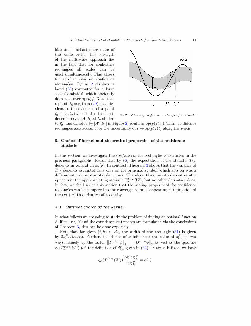
Fig 2. Obtaining confidence rectangles from bands.

bias and stochastic error are ofthe same order. The strengthof the multiscale approach liesin the fact that for confidencerectangles all scales can beused simultaneously. This allowsfor another view on confidencerectangles. Figure 2 displays aband (33) computed for a largescale/bandwidth which obviouslydoes not cover op(p)f . Now, takea point, t0 say, then (29) is equiv-alent to the existence of a pointt′0 ∈ [t0, t0+h] such that the confi-dence interval [A,B] at t0 shiftedto t′0 (and denoted by [A′, B′] in Figure 2) contains op(p)f(t′0). Thus, confidencerectangles also account for the uncertainty of t 7→ op(p)f(t) along the t-axis.

5. Choice of kernel and theoretical properties of the multiscalestatistic

In this section, we investigate the size/area of the rectangles constructed in theprevious paragraphs. Recall that by (6) the expectation of the statistic Tt,hdepends in general on op(p). In contrast, Theorem 3 shows that the variance ofTt,h depends asymptotically only on the principal symbol, which acts on φ as adifferentiation operator of order m+ r. Therefore, the m+ r-th derivative of φappears in the approximating statistic TP,∞n (W ), but no other derivative does.In fact, we shall see in this section that the scaling property of the confidencerectangles can be compared to the convergence rates appearing in estimation ofthe (m+ r)-th derivative of a density.

5.1. Optimal choice of the kernel

In what follows we are going to study the problem of finding an optimal functionφ. If m+r ∈ N and the confidence statements are formulated via the conclusionsof Theorem 3, this can be done explicitly.

Note that for given (t, h) ∈ Bn, the width of the rectangle (31) is givenby 2dPt,h/(h

√n). Further, the choice of φ influences the value of dPt,h in two

ways, namely by the factor∥∥Dr+m

+ φ∥∥2

=∥∥Dr+mφ

∥∥2

as well as the quantile

qα(TP,∞n (W )) (cf. the definition of dPt,h given in (32)). Since α is fixed, we have

qα(TP,∞n (W ))log log ν

h

log νh

= o(1).


Therefore, dPt,h depends in first order on∥∥Dr+mφ

∥∥2

and our optimization prob-lem can be reformulated as

minimize∥∥Dr+mφ

∥∥2, subject to

∫φ(u)du = 1.

This is in fact easy to solve if we additionally assume that φ ∈ Hq with r +m ≤ q < r + m + 1/2. By Lagrange calculus, we find that on (0, 1), φ hasto be a polynomial of order 2m + 2r. Under the induced boundary conditionsφ(k)(0) = φ(k)(1) = 0 for k = 0, . . . , r +m− 1, the solution φm+r is of the form

φm+r(x) = cm+rxm+r(1− x)m+rI(0,1)(x). (34)

Due to the normalization constraint∫φm+r(u)du = 1, it follows that φm+r is the

density of a beta distributed random variable with parameters α = m+r+1 andβ = m+r+1, implying, cm+r = (2m+2r+1)!/((m+r)!)2. It is worth mentioning

that φ(m+r)m+r , restricted to the domain [−1, 1), is (up to translation/scaling) the

(m+ r)-th Legendre polynomial Lm+r, i.e.

φ(m+r)m+r = (−1)m+r (2m+ 2r + 1)!

(m+ r)!Lm+r(2 · −1)

(this is essentially Rodrigues’ representation, cf. Abramowitz and Stegun [1], p.785). For that reason, we even can compute

∥∥φ(m+r)m+r

∥∥L2 =

(2m+ 2r)!

(m+ r)!

√2m+ 2r + 1.

In the particular case r = 0, m = 1 we obtain φ(1)1 (x) ∝ 1 − 2x. This is

known from the work of Dumbgen and Walther [14] who considered locally

most powerful tests to derive φ(1)1 .

To summarize, we can find the “optimal” kernel but it turns out that it hasless smoothness than it is required by the conditions for Theorem 3 due to itsbehavior on the boundaries {0, 1}. However, if the operator defining the shapeconstraint and the inversion operator g 7→ f are both differential operators (foran example see Section 1.1), then, the theorems can be proved under weakerassumptions on φ including as a special case the optimal beta kernels.

5.2. Theoretical properties of the method

In this part, we give some theoretical insights. We start by investigating Problem(iii) (cf. Section 3). After that, we will address issues related to (ii) and (i).It is easy to see that ‖vt,h‖2 . h1/2−m−r and thus, dt,h and dPt,h are of thesame order. We can therefore restrict ourselves in the following to the situation,where the confidence statements are constructed based on the approximation inTheorem 2. In the other case, similar results can be derived.


Problem (iii): Recall that with confidence 1− α, for all (t, h) ∈ Bn,

graph(op(p)f) ∩[t, t+ h

]×[Tt,h − dt,h

h√n

,Tt,h + dt,hh√n

]6= ∅.

The so constructed rectangles localize op(p)f , where the amount of informationis directly linked to the size of the rectangle. Therefore, it is natural to thinkof the length of the diagonal as a measure of localization quality. This lengthbehaves like h ∨ h−m−r−1/2n−1/2

√log 1/h. In particular, if the rectangle is a

square, then, h ∼ (log n/n)1/(3+2m+2r) and this coincides with the optimalbandwidth for a kernel density estimator under a Lipschitz assumption on f .This is no surprise, of course, since Lipschitz continuity allows a function tooscillate over an interval I by an amount that is proportional to the length |I|.

Problem (ii), (ii′): The following lemma gives a necessary condition in orderto solve (ii). Loosely speaking, it states that whenever

op(p)f∣∣[t,t+h]

& n−1/2h−m−r−1/2√

log 1/h,

the multiscale test returns a rectangle [t, t + h] × [b−(t, h, α), b+(t, h, α)] whichis in the upper half-plane with high-probability. Or, to state it differently, wecan reject that op(p)f

∣∣[t,t+h]

< 0.

In order to formulate the next theorem, recall the definition of b±(t, h, α)given in (30). Further, set rt,h,n := 2dt,h/(h

√n) and denote by M−n the set

of tupels (t, h) ∈ Bn for which op(p)f∣∣[t,t+h]

> rt,h,n. Similarly define M+n :=

{(t, h) ∈ Bn | op(p)f |[t,t+h] < −rt,h,n}.

Theorem 4. Work under the assumptions of Theorem 2. If φ ≥ 0, then

limn→∞

P(

(−1)∓b±(t, h, α) > 0, for all (t, h) ∈M±n)≥ 1− α.

Proof. For all (t, h) ∈M−n , conditionally on the event given by (28),

op(p)f∣∣[t,t+h]

> rt,h,n ⇒ 〈φt,h, op(p)f〉 > hrt,h,n

⇒ Tt,h > dt,h ⇒ b−(t, h, α) > 0.

One can argue similarly for M+n .

Define

Cα :=(√

8‖fε‖∞hm+r−1/2‖vt,h‖2(1 + qα(T∞n (W ))))2/(2m+2r+1)

(35)

and let M± be the set of tupels (t, h) ∈ Bn satisfying the pair of constraints

h ≥ Cα(

log n

n

)1/(2β+2m+2r+1)


and

op(p)f∣∣[t,t+h]

≶

(log n

n

)β/(2β+2m+2r+1)

(36)

(with > in the last equality corresponding to M−n and < to M+n ).

Corollary 1. Work under the assumptions of Theorem 2. If φ ≥ 0 and β ∈ R,then

limn→∞

P(

(−1)∓b±(t, h, α) > 0, for all (t, h) ∈ M±n)≥ 1− α.

Proof. It holds that

dt,h ≤ ‖fε‖1/2∞∥∥vt,h∥∥2√2 log ν/h

(1 + qα(T∞n (W ))

).

For sufficiently large n, h ≥ ln ≥ ν/n. Therefore we have for every (t, h) ∈ M−n ,

rt,h,n ≤√

8 ‖fε‖∞∥∥vt,h∥∥2(1 + qα(T∞n (W ))

)h−1/2n−1/2

√log n < op(p)f

∣∣[t,t+h]

.

Similar for M+n . Since M±n ⊂ M±n , the result follows directly from Theorem

4.

Roughly speaking, the last result shows that if h ∼ (log n/n)1/(2β+2m+2r+1)

and op(p)f∣∣[t,t+h]

∼ (log n/n)β/(2β+2m+2r+1) = hβ , then with probability 1−α,

our method returns a rectangle in the upper half-plane. We have three distinctregimes

β > 0 : op(p)f∣∣[t,t+h]

→ 0,

β = 0 : op(p)f∣∣[t,t+h]

= O(1),

−m− r − 12 < β < 0 : op(p)f

∣∣[t,t+h]

→∞.

It is insightful to compare the previous result to derivative estimation of adensity if m+r is a positive integer. As it is well known, Dm+rf can be estimatedwith rate of convergence ( log n

n

)β/(2β+2m+2r+1)

under L∞-risk assuming that op(p)f is Holder continuous with index β > 0 andh ∼ (log n/n)1/(2β+2m+2r+1). This directly relates to the first case consideredabove.

Problem (i): At the beginning of Section 3 we shortly addressed constructionof confidence statements for the number of roots and their location. Note thatestimators derived in this way, have many interesting features. On the one hand,we know that with probability 1 − α the estimated number of roots is a lowerbound for the true number of roots. Therefore, these estimates do not comefrom a trade-off between bias and variance but they allow for a clear control on


the probability to observe artefacts. In order to show that the lower bound forthe number of roots is not trivial, we need to prove that whenever two roots arewell-separated (for instance the distance between them shrinks not too fast),they will be detected eventually by our test. This property follows if we canshow that the simultaneous confidence intervals for a fixed number of roots, say,shrink to zero.

Therefore, assume for simplicity that the numberK and the locations (x0,j)j=1,...,K

of the zeros of op(p)f are fixed (but unknown) and x0,j ∈ (0, 1) for j = 1, . . . ,K.For example, these roots can be extreme/saddle points if op(p) = D or pointsof inflection if op(p) = D2.

In order to formulate the result, we need thatBn is sufficiently rich. Therefore,we assume that for all n, there exists a sequence (Nn), Nn & n1/(2m+2r+1) log4 n,such that{( k

Nn,l

Nn

) ∣∣ k = 0, 1, . . . , l = 1, 2, . . . , k + l ≤ Nn}⊂ Bn.

Assume further that in a neighborhood of the roots x0,j , op(p)f behaves like

op(p)f(x) = γ sign(x− x0,j)|x− x0,j |β + o(|x− x0,j |β),

for some positive β ∈ (0, 1]. Let ρn = (log n/n)1/(2β+2m+2r+1)2/γ1/β and Cα,M±n

as defined in Corollary 1. There exist integer sequences (k−j,n)j,n, (k+j,n)j,n, (ln)nsuch that for all sufficiently large n,

ρn ≤k−j,nNn− x0,j ≤ 2ρn, −2ρn ≤

k+j,nNn− x0,j ≤ −ρn,

and

Cαγ1/βρn ≤

lnNn≤ 2Cαγ

1/βρn.

Direct calculations show (k−j,n/Nn, ln/Nn) ∈M−n and ((k+j,n − ln)/Nn, ln/Nn) ∈M+n for j = 1, . . . ,K. We can conclude from Corollary 1 and the construction

that for j = 1, . . . ,K, the confidence intervals have to be a subinterval of[k+j,n − lnNn

,k−j,n + ln

Nn

].

Hence, the length for each confidence interval is bounded from above by

4(Cαγ1/β + 1)ρn ∼

(log n

n

)1/(2β+2m+2r+1)

.

As n → ∞ the confidence intervals shrink to zero, and will therefore becomedisjoint eventually. This shows that our estimator for the number of roots picksasymptotically the correct number with high probability. Observe, that for local-ization of modes in density estimation (m, r, β) = (1, 0, 1) the rate (log n/n)1/5 is


indeed optimal up to the log-factor (cf. Hasminskii [24]). The rate (log n/n)1/7

for localization of inflection points in density estimation (m, r, β) = (2, 0, 1)coincides with the one found in Davis et al. [9].

For the special case of mode estimation in density deconvolution (here: (m, r, β) =(1, r, 1)) let us shortly comment on related work by Rachdi and Sabre [42] andWieczorek [45]. In [45] optimal estimation of the mode under relatively restric-tive conditions on the smoothness of f is considered. In contrast, Rachdi andSabre find the same rates of convergence n−1/(2r+5) (but with respect to themean-square error). Under the stronger assumption that D3f exists they alsoprovide confidence bands which converge at a different rate, of course.

5.3. On calibration of multiscale statistics

Let us shortly comment on the type of multiscale statistic, derived in Theorems1-3. Following [13], p.139, we can view the calibration of the multiscale statistics(11), (22), and (26) as a generalization of Levy’s modulus of continuity. In fact,the supremum is attained uniformly over different scales, making this calibrationin particular attractive for construction of adaptive methods.

One of the restrictions of our method, compared to other works on multi-scale statistics, is that we exclude the coarsest scales, i.e. h > un = o(1) (cf.Theorem 1). Otherwise the approximating statistic would not be distribution-free. However, excluding the coarsest scales is a very weak restriction since theimportant features of op(p)f can be already detected at scales tending to zerowith a certain rate. For instance in view of Corollary 1, the multiscale methoddetects a deviation from zero, i.e. op(p)f

∣∣I≥ C > 0, provided the length of the

interval I is larger than const.× (log n/n)1/(2m+2r+1). This can be also seen bynumerical simulations, as outlined in the next section.

6. Numerical simulations

In this section we provide further simulation results and discussion to the ex-ample from Section 1.1 (cf. also Example 1, Section 3), that is, studying mono-tonicity of the density f under Laplace-deconvolution. More precisely, the errordensity is fε(x) = θ−1e−|x|/θ with θ = 0.075. In this case,

F(fε)(t) = 〈θt〉−2 and op(p)?f = −Df.

One should notice that for Laplace deconvolution the inversion operator, map-ping g to f , is given by 1−θ2D2 and therefore the statistic (19) takes the simpleform (2) (cf. also the discussion following Theorem 2). The ill-posedness of theshape constraint and the deconvolution problem give m = 1, r = 2. Togetherwith (34) it is therefore natural to choose φ as the density of a Beta(4, 4) randomvariable. Further, recall that un = 1/ log log n, Nn = [n3/5], and

Bn ={( k

Nn,l

Nn

) ∣∣ k = 0, 1, . . . , l = 1, 2, . . . , [Nnun], k + l ≤ Nn}.


Fig 3. Boxplots for three different values (n = 200, n = 1000, n = 10.000) of the approxi-mating statistic (37).

Note that Assumptions 3 and 4 hold for (A, ρ, r, β0) = (θ2, 0, 2, 2) and (µ,m) =(1, 1), respectively. Thus, we might work in the framework of Theorem 3. Themultiscale statistics

TPn = sup(t,h)∈Bn

wh

(|Tt,h − ETt,h|√gn(t) θ2 ‖φ(3)‖2

−√

2 log(νh

))

and

TP,∞n (W ) = sup(t,h)∈Bn

wh

(∣∣ ∫ φ(3)( s−th )dWs

∣∣√h ‖φ(3)‖2

−√

2 log(νh

))(37)

have a particular simple form as well and the rectangles in (31) can be computedvia

dPt,h = h−5/2√gn(t)θ2‖φ(3)‖2

√2 log ν

h

(1 + qα,n

log logνh

logνh

). (38)

Boxplots for the distributions TP,∞200 (W ), TP,∞1000 (W ) and TP,∞10.000(W ) are displayedin Figure 3 based on 10.000 repetitions each. The plot shows that the distributionis well-concentrated with a few outliers only. Although our theoretical resultsimply boundedness of the multiscale statistic as n→∞, Figure 3 indicates thatif n is in the range of a few thousands TP,∞n (W ) increases slowly.

In Section 1.1 we showed confidence statements for a simulated sample ofsize n = 2000. To complement our study, let us now investigate the case oflarge n, i.e. n = 10.000. Again we choose the confidence level equal to 90%.The estimated quantile is q0.1(TP,∞10.000(W )) = −0.04. For all simulations, we use

ν = exp(e2) because then, h 7→√

log ν/h/(log log ν/h) is monotone as long as0 < h ≤ 1 (cf. Lemma B.11 (i)). The density f has been designed in order toinvestigate Corollary 1 numerically. Indeed, on [0, 0.35] the signal |f ′| is largeon average, but the intervals on which f increases/decreases are comparably


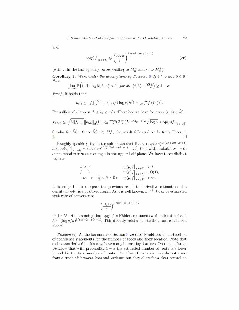
Fig 4. Simulation for sample size n = 10.000 and 90%-quantile. Upper display: True densityf (dashed) and convoluted density g (solid). Lower display: Subset of minimal solutions to(ii) and (ii′) (horizontal lines above/below the thin line)

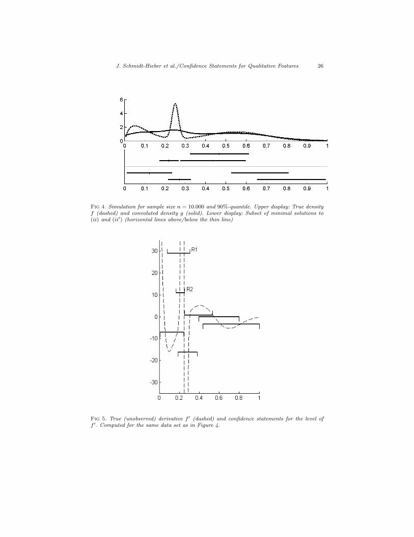
Fig 5. True (unobserved) derivative f ′ (dashed) and confidence statements for the level off ′. Computed for the same data set as in Figure 4.


small. By way of contrast, on [0.35, 1] the signal |f ′| is small and there is onlyone increase/decrease.

The test is able to find all increases and decreases of f besides the increaseon [0, 0.04], which is not detected (cf. Figure 4). In contrast to the simulation inFigure 1, we see now a much better localization of the sharp increase/decreaseon [0.2, 0.25] and [0.25, 0.3].

With the confidence rectangles at hand, we are able to say more about fthan localizing regions of increase/decrease only. In fact, we also can providesome confidence statements about the value of f ′ close to a given point. Insteadof plotting all confidence statements, we have displayed in Figure 5 the mostprominent ones, allowing for a good characterization of the derivative f ′ andtelling us something about the strength of the increases/decreases of f .A bracket of type “t” means that f ′ has to be above the horizontal line, some-where. To give an example, from the bracket R1 we can conclude that at leaston a subset of [0.07, 0.3], the derivative f ′ exceeds 29. Similarly, “u” means thatsomewhere f ′ has to be below the corresponding horizontal line. As always,these statements hold simultaneously with confidence 90%.

What we find is that in regions where the derivative does not oscillate much,we can achieve rather precise confidence statements about the value of f ′. Forexample, from the rightmost bracket we can infer that with confidence 90%the minimum of f ′ on [0.45, 1] has to be below −4, coming close to the trueminimum, which is approximately −6.

Figure 5 also shows nicely why a multiscale approach can provide additionalinsight compared to a one-scale method. Consider R1 and R2 in Figure 5 anddenote by (t1, h1) and (t2, h2) the corresponding indices in Bn (as in (31)).Note that R1 and R2 belong to similar time points in the sense that R2 ⊂R1 but different bandwidths h1, h2. Therefore we may view R1 and R2 as asuperposition of confidence statements on different scales. This allows to inferdifferent qualitative and quantitative statements close to the same time point.We would use R2 in order to detect and localize an increase (as in Figure 4) orto construct a confidence band for a mode, whereas from R1 we obtain a betterlower bound for sup f ′. Thus, for a qualitative analysis there is a real gain bytaking into account all scales simultaneously.

7. Outlook and Discussion

Given a density deconvolution model, we have investigated multiscale meth-ods in order to analyze qualitative features of the unknown density which canbe expressed as pseudo-differential operator inequalities. Compared to previouswork, a more refined multiscale calibration has been considered using an ideaof proof based on KMT results together with tools from the theory of pseudo-differential operators. We believe that the same strategy can be applied to avariety of other problems. In particular, it is to be expected that similar resultswill hold for regression and spectral density estimation.

In the formulation of the problem but also in the proofs it becomes appar-ent that modern tools from functional and harmonic analysis such as pseudo-


differential operators are very helpful and to a certain extent unavoidable. In thesame spirit, very recently, Nickl and Reiß [40] as well as Sohl and Trabs [43] usedsingular integral theory in order to prove Donsker theorems in deconvolution-type models. It is expected that reconsidering deconvolution theory from theviewpoint of harmonic analysis will lead to an improved understanding of thefield.

Our multiscale approach allows us to identify intervals such that for givensignificance level we know that op(p)f > 0 at least on a subinterval. As out-lined in Section 5, these results allow for qualitative inference as for exampleconstruction of confidence bands for the roots of op(p)f . Since we only requiredthat op(p)f is continuous, op(p)f can be highly oscillating. In this framework, itis therefore impossible to obtain strong confidence statements in the sense thatwe find intervals on which op(p)f is always positive. By adding bias controllingsmoothness assumptions such as for instance Holder conditions stronger resultscan be obtained resulting for instance in uniform confidence bands.

Obtaining multiscale results for error distributions as in Assumption 2 isalready a very difficult topic on its own and extension to the severely ill-posedcase, including Gaussian deconvolution, becomes technically challenging sincethe theory of pseudo-differential operators has to the best of our knowledge notbeen formulated on the induced function spaces so far. Therefore we intend totreat this in a subsequent paper.

Restricting to shape constraint which are associated with pseudo-differentialoperators appears to be a limitation of our method, since important shape con-straints as for instance curvature cannot be handled within this framework andwe may only work with linearizations (which is quite common in physics andengineering). Allowing for non-linearity is a very challenging task for furtherinvestigations. We are further aware of the fact that many other importantqualitative features are related to integral transforms (that are in general not ofconvolution type) and they do not have a representation as pseudo-differentialoperator. For instance complete monotonicity and positive definiteness are byBernstein’s and Bochner’s Theorem connected to the Laplace transform andFourier transform, respectively. They cannot be handled with the methods pro-posed here and are subject to further research.

Acknowledgments. This research was supported by the joint research grantFOR 916 of the German Science Foundation (DFG) and the Swiss National Sci-ence Foundation (SNF). The first author was partly funded by DFG postdoc-toral fellowship SCHM 2807/1-1. The second author would like to acknowledgesupport by DFG grants CRC 755 and CRC 803. The authors are grateful forvery helpful comments by Steve Marron, Markus Reiß , Jakob Sohl, MathiasTrabs, and Gunther Walther as well as two referees and an associate editorwhich led to a more general version of previous results.


Appendix A Proofs of the main theorems

Throughout the appendix, let

wh =

√12 log ν

h

log log νh

, wh =log ν

h

log log νh

.

Furthermore, we often use the normalized differential –dξ := (2π)−1dξ

Proof of Theorem 1. In a first step we study convergence of the statistic

T (1)n = sup

(t,h)∈Bnwh

∣∣Tt,h − ETt,h∣∣

Vt,h√g(t)

− wh.

Note that T(1)n is the same as Tn, but gn is replaced by the true density g. We

show that there exists a (two-sided) Brownian motion W , such that with

T (2)n (W ) := sup

(t,h)∈Bnwh

∣∣ ∫ ψt,h(s)√g(s)dWs

∣∣Vt,h

√g(t)

− wh,

we have

supG∈Gc,C,q

∣∣T (1)n − T (2)

n (W )∣∣ = oP (rn). (39)

The main argument is based on the standard version of KMT (cf. [33]). Thisis a fairly classical result, but has never been used to describe the asymptoticdistribution of a multiscale statistic, the only exception being Walther [44]. Inorder to state the result, let us define a Brownian bridge on the index set [0, 1]as a centered Gaussian process (B(f)){f∈F}, F ⊂ L2([0, 1]) with covariancestructure

Cov(B(f), B(g)

)= 〈f, g〉 − 〈f, 1〉〈g, 1〉.

For F0 := {x 7→ I[0,s](x) : s ∈ [0, 1]}, the process (B(f)){f∈F0} coincides withthe classical definition of a Brownian bridge. If Ui ∼ U [0, 1], i.i.d., the uniformempirical process on the function class F is defined as

Un(f) =√n( 1

n

n∑i=1

f(Ui)−∫f(x)dx

), f ∈ F .

In particular

Tt,h − ETt,h = Un(ψt,h ◦G−1

),

where G−1 denotes the quantile function of Y . For convenience, we restate thecelebrated KMT inequality for the uniform empirical process.


Theorem 5 (KMT on [0, 1], cf. [33]). There exist versions of Un and a Brownianbridge B such that for all x

P(

supf∈F0

∣∣Un(f)−B(f)∣∣ > n−1/2(x+ C log n)

)< Ke−λx,

where C,K, λ > 0 are universal constants.

However, we need a functional version of KMT. We shall prove this by usingthe theorem above in combination with a result due to Koltchinskii [32], (The-orem 11.4, p. 112) stating that the supremum over a function class F behavesas the supremum over the symmetric convex hull sc(F), defined by

sc(F) :={ ∞∑i=1

λifi : fi ∈ F , λi ∈ [−1, 1],

∞∑i=1

|λi| ≤ 1}.

Theorem 6. Assume there exists a version B of a Brownian bridge, such thatfor a sequence (δn)n tending to 0,

P∗(

supf∈F|Un(f)−B(f)| ≥ δn(x+ C log n)

)≤ Ke−λx,

where C,K, λ > 0 are constants depending only on F . Then, there exists aversion B of a Brownian bridge, such that

P∗(

supf∈sc(F)

|Un(f)− B(f)| ≥ δn(x+ C ′ log n))≤ K ′e−λ

′x

for constants C ′,K ′, λ′ > 0.

In Theorem 6, P? refers to the outer measure, however, for the function classconsidered in this paper, we have measurability of the corresponding event andhence may replace P? by P. It is well-known (cf. Gine et al. [19], p. 172) that{

ρ∣∣ ρ : R→ R, supp ρ ⊂ [0, 1], ρ(1) = 0, TV(ρ) ≤ 1

}⊂ sc(F0). (40)

Now, assume that ρ : R → R is such that TV(ρ) + 3|ρ(1)| ≤ 1. Define ρ =(ρ − ρ(1)I[0,1])/(1 − |ρ(1)|) and observe that TV(ρ) ≤ 1 and ρ(1) = 0. By (40)there exists λ1, λ2, . . . ∈ R and t1, t2, . . . ∈ [0, 1] such that ρ =

∑λiI[0,ti] and∑

|λi| ≤ 1. Therefore, ρ = (1 − |ρ(1)|)ρ + ρ(1)I[0,1] can be written as linearcombination of indicator functions, such that the sum of the absolute values ofweights is bounded by 1. This shows{

ρ∣∣ ρ : R→ R, supp ρ ⊂ [0, 1], TV(ρ) + 3|ρ(1)| ≤ 1

}⊂ sc(F0).

Since TV(ψt,h ◦ G−1) ≤ TV(ψt,h) it follows by Assumption 1 (ii) that thefunction class

Fn :={C?V

−1t,h

√h ψt,h ◦G−1 : (t, h) ∈ Bn, G ∈ Gc,C,q

}


is a subset of sc(F0) for sufficiently small constant C?. Combining Theorems 5

and 6 shows for δn = n−1/2 that there are constants C ′,K ′, λ′ and a Brownianbridge (B(f))f∈sc(F0) such that for x > 0, the probability of{

sup(t,h)∈Bn, G∈G

C?

√h∣∣Un(ψt,h ◦G−1)−B(ψt,h ◦G−1)∣∣

Vt,h≥ 1√

n(x+ C ′ log n)

}is bounded by K ′e−λ

′x. Due to Lemma B.11 (i) and ln ≥ ν/n for sufficientlylarge n, we have that wln ≤ wν/n. This readily implies with x = log n that


wh

∣∣∣∣∣Tt,h − ETt,h∣∣− ∣∣B(ψt,h ◦G−1)∣∣∣∣∣

Vt,h√g(t)

= OP

( 1√lnn

wν/n log n).

Now, let us introduce the (general) Brownian motion W (f) as a centered Gaus-sian process with covariance E[W (f)W (g)] = 〈f, g〉. In particular, W (f) =B(f) + (

∫f)ξ, ξ ∼ N (0, 1) and independent of B, defines a Brownian mo-

tion and hence there exists a version of (W (f))f∈sc(F0) such that B(f) =W (f)− (

∫f)W (1). We have


wh

∣∣ ∫ ψt,h(u) dG(u)∣∣

Vt,h√g(t)

≤ c−1 sup(t,h)∈Bn, G∈G

wh‖ψt,h‖1

Vt,h√g(t)

. suph∈[ln,un]

whh1/2 ≤ wunu1/2n ,

where the second inequality follows from Assumption 1 (ii) and the last inequal-ity from Lemma B.11 (ii). This implies further

E[∥∥∥ wh

Vt,h√g(t)

[∣∣B(ψt,h ◦G−1)∣∣− ∣∣W (ψt,h ◦G−1)∣∣]∥∥∥Fn

]= O(wunu

1/2n ),

and therefore

supG∈G

∣∣∣T (1)n − sup

(t,h)∈Bnwh

∣∣W (ψt,h ◦G−1)∣∣Vt,h

√g(t)

− wh∣∣∣ = OP (

w1/n log n√lnn

+ wunu1/2n ),

and

supG∈G

∣∣∣T (1)n − T (2)

n (W )∣∣∣ = OP (l−1/2n n−1/2w1/n log n+ wunu

1/2n ).

In the last equality we used that (W(1)t )t∈[0,1] = (W (I[0,t](·)))t∈[0,1] and

(Wt)t∈R =(∫ t

0

I{g>0}(s)√g(s)

dW(1)G(s)

)t∈R

are (two-sided) standard Brownian motions, proving W (ψt,h ◦ G−1) =∫ψt,h(s)

√g(s)dWs and hence (39). Further note that Assumption 1 (iii) to-

gether with Lemma B.10 shows that

supG∈G

∣∣∣T (2)n (W )− sup

(t,h)∈Bnwh

∣∣ ∫ ψt,h(s)dWs

∣∣Vt,h

− wh∣∣∣ = OP (κn).


In a final step let us show that (13) is almost surely bounded. In order to estab-lish the result, we use Theorem 6.1 and Remark 1 of Dumbgen and Spokoiny[13]. We set ρ

((t, h), (t′, h′)

)= (|t − t′| + |h − h′|)1/2. Further, let X(t, h) =√

hV −1t,h

∫ψt,h(s)dWs and σ(t, h) = h1/2.

By assumption, X has continuous sample paths on T and obviously, for all(t, h), (t′, h′) ∈ T ,

σ2(t, h) ≤ σ2(t′, h′) + ρ2((t, h), (t′, h′)).

Let Z ∼ N (0, 1). Since X(t, h) is a Gaussian process and Vt,h ≥ ‖φt,h‖2,P(X(t, h) > σ(t, h)η) ≤ P(Z > η) ≤ exp(−η2/2) for any η > 0. Further, denoteby

At,t′,h,h′ :=

∥∥∥∥∥ψt,h√h

Vt,h− ψt′,h′

√h′

Vt′,h′

∥∥∥∥∥2

. (41)

Because of P(|X(t, h) − X(t′, h′)∣∣ ≥ At,t′,h,h′η

)≤ 2 exp

(− η2/2

)we have by

Lemma B.6 for a universal constant K > 0,

P(∣∣X(t, h)−X(t′, h′)

∣∣ ≥ ρ((t, h), (t′, h′))η)≤ 2 exp

(− η2/(2K2)

).

Finally, we can bound the entropy N ((δu)1/2, {(t, h) ∈ T : h ≤ δ}) similarly asin [13], p. 145. Therefore, application of Remark 1 in [13] shows that

S := sup(t,h)∈T

√12 log e

h


∣∣log(e log e

h

)Vt,h

−

√log( 1

h ) log( eh )

log(e log e

h

)is almost surely bounded from above. Define

S′ := sup(t,h)∈T

√12 log ν

h


∣∣log log ν

h Vt,h−

√log( 1

h ) log( νh )

log log νh

.

If e < ν ≤ ee, then

log log νh = log

(log νe log ee

he/ log ν

)≥ log log ν − 1 + log

(e log e

h

)implies

log(e log e

h

)log log ν

h

≤ 1

log log ν+ 1.

Furthermore, log ν/h ≤ (log ν)(log e/h). Suppose now that S′ > 0 (otherwiseS′ is bounded from below by 0). Then, S′ . S and hence S′ is almost surelybounded. Finally, √

log νh

∣∣√log 1h −

√log ν

h

∣∣ ≤ log ν.


Therefore, (13) holds, i.e.

sup(t,h)∈T

wh


∣∣Vt,h

− wh

is almost surely bounded.

In the last step, it remains to prove that supG∈Gc,C,q |Tn−T(1)n | = OP (supG∈G ‖gn−

g‖∞ log n/ log log n). For sufficiently large n and because G ∈ G, gn ≥ c/2 forall t ∈ [0, 1]. Therefore using Lemma B.11 (i),

supG∈G

∣∣Tn − T (1)n | ≤ sup

(t,h)∈Bn, G∈Gwh

∣∣Tt,h − E[Tt,h]∣∣

Vt,h√g(t)

supG∈G∥∥gn − g∥∥∞gn(t)

≤2 supG∈G

∥∥gn − g∥∥∞c


wh

∣∣Tt,h − E[Tt,h]∣∣

Vt,h√g(t)

≤2 supG∈G

∥∥gn − g∥∥∞c

(T (1)n + sup

h∈[ln,un]wh)

≤2 supG∈G

∥∥gn − g∥∥∞c

(T (1)n +O(

log n

log log n)). (42)

Since T(1)n is a.s. bounded by Theorem 1, the result follows.

Remark 1. Next, we give a proof of Theorem 2. In fact we proof a slightlystronger version, which does not necessarily require the symbol a to be ellipticand Vt,h = ‖vt,h‖2. It is only assumed that

(i) Vt,h ≥ ‖vt,h‖2,(ii) there exists constants cV , CV with 0 < cV ≤ hm+r−1/2Vt,h ≤ CV <∞

(iii) for all (t, h), (t′, h′) ∈ T and whenever h ≤ h′ it holds that hm+r|Vt,h −Vt′,h′ | ≤ CV (|t− t′|+ |h− h′|)1/2.

As a special case these conditions are satisfied for Vt,h = ‖vt,h‖2 and op(a)elliptic. This follows directly from Lemmas B.3 and B.5.

Proof of Theorem 2. In order to prove the statements it is sufficient to checkthe conditions of Theorem 1. For h > 0 define the symbol

a?t,h(x, ξ) := hma?(xh+ t, h−1ξ). (43)

Under the imposed conditions and by Remark B.1 we may apply Lemma B.2for a(t,h) = a?t,h and therefore, uniformly over (t, h) ∈ T and u, u′ ∈ R,

(I) |vt,h(u)| . h−m−r min(1, h2

(u−t)2).

(II) |vt,h(u)− vt,h(u′)| . h−m−r−1|u− u′| and if u, u′ 6= t,

|vt,h(u)− vt,h(u′)| . h1−m−r|u− u′|

|u′ − t| |u− t|= h1−m−r

∣∣ ∫ u

u′

1

(x− t)2dx∣∣.


Using (I), we obtain ‖vt,h‖∞ . h−m−r and ‖vt,h‖1 . h1−m−r. In order toshow that the total variation is of the right order, let us decompose vt,h further

into v(1)t,h = vt,hI[t−h,t+h] and v

(2)t,h = vt,h − v(1)t,h . By (II), TV(v

(1)t,h) . h−m−r and

TV(v(2)t,h) . h−m−r + h1−m−r

∫ ∞t+h

1

(x− t)2dx . h−m−r.

Since TV(vt,h) ≤ TV(v(1)t,h) + TV(v

(2)t,h) . h−m−r, this shows together with

Remark 1 that part (ii) of Assumption 1 is satisfied.Next, we verify Assumption 1, (iii) with κn = sup(t,h)∈Bn whh

1/2 log(1/h) .

u1/2n log3/2 n (cf. Lemma B.11, (ii)), i.e. we show


whTV

(vt,h(·)[

√g(·)−

√g(t)]〈·〉α

)Vt,h

. u1/2n log3/2 n.

By Lemma B.12, we see that this holds for vt,h replaced by v(1)t,h . Therefore,

it remains to prove the statement for v(2)t,h . Let us decompose v

(2)t,h further into

v(2,1)t,h = vt,hI[t−1,t+1]∩[t−h,t+h]c and v

(2,2)t,h = v

(2)t,h−v

(2,1)t,h = vt,hI[t−1,t+1]c . For the

remaining part, let u, u′ be such that |u− t| ≥ |u′ − t| ≥ h. We have

TV(v(2,1)t,h (·)

[√g(·)−

√g(t)

]〈·〉α

).∥∥v(2,1)t,h (·)

[√g(·)−

√g(t)

]∥∥∞

+ TV(v(2,1)t,h (·)

[√g(·)−

√g(t)

]). (44)

Using (I) and (II) together with the properties of the class G we can bound the

variation∣∣v(2,1)t,h (u)

[√g(u)−

√g(t)

]− v(2,1)t,h (u′)

[√g(u′)−

√g(t)

]∣∣ by∣∣v(2,1)t,h (u)− v(2,1)t,h (u′)∣∣ · ∣∣√g(u′)−

√g(t)

∣∣+∣∣v(2,1)t,h (u)

∣∣ · ∣∣√g(u)−√g(u′)

∣∣. h1−m−r |u−u

′||u−t| + h2−m−r |u−u

′||u−t|2 . h1−m−r |u−u

′||u−t| ≤ h

1−m−r∣∣ ∫ u

u′

1|x−t|dx

∣∣.Due to h ≥ ln & 1/n this yields

TV(v(2,1)t,h (·)[

√g(·)−

√g(t)]

). h1−m−r + h1−m−r

∫ t+1

t+h

du

|u− t|. h1−m−r log 1

h . h1−m−r log n

and with (44) also

TV(v(2,1)t,h (·)

[√g(·)−

√g(t)

]〈·〉α

). h1−m−r log n. (45)

Finally, let us address the total variation term involving v(2,2)t,h . Given Gc,C,q we

can choose α such that α > 1/2 and α + q < 1 (recall that 0 ≤ q < 1/2). ByLemma B.7, we find that∣∣v(2,2)t,h (u)〈u〉α − v(2,2)t,h (u′)〈u′〉α

∣∣ . h1−m−r∣∣∣ ∫ u

u′

1

(x− t)2−α+

1

(x− t)2dx∣∣∣.


Moreover

〈u〉α(1 + |u′|+ |u|)q ≤ (1 + |u′|+ |u|)q+α

≤ (3 + 2|u− t|)q+α ≤ 3 + 2|u− t|q+α

and thus∣∣v(2,2)t,h (u)〈u〉α∣∣ ∣∣√g(u)−

√g(u′)

∣∣ . h2−m−r|u− t|q+α + 1

|u− t|2|u− u′|.

This allows us to bound the variation by∣∣v(2,2)t,h (u)[√

g(u)−√g(t)

]〈u〉α − v(2,2)t,h (u′)

[√g(u′)−

√g(t)

]〈u′〉α

∣∣≤∣∣v(2,2)t,h (u)〈u〉α

∣∣ ∣∣√g(u)−√g(u′)

∣∣+2√c

∣∣v(2,2)t,h (u)〈u〉α − v(2,2)t,h (u′)〈u′〉α∣∣

. h1−m−r∣∣∣ ∫ u

u′

1

(x− t)2−q−α+

1

(x− t)2−α+

1

(x− t)2dx∣∣∣

and therefore we conclude that

TV(v(2,2)t,h (·)

[√g(·)−

√g(t)

]〈·〉α

). h1−m−r + h1−m−r

∫ ∞t+1

1

(x− t)2−q−α+

1

(x− t)2−α+

1

(x− t)2dx

≤ h1−m−r.

Together with the bound for v(1)t,h and (45) this yields Assumption 1, (iii).

Finally, Assumption 1 (iv) follows from Lemma B.5 and Remark 1 due toφ ∈ Hdr+me ∩ Hr+m+1/2, suppφ ⊂ [0, 1] and φ ∈ TV(Ddr+meφ) < ∞. Thisshows that Assumption 1 holds for (vt,h, Vt,h).

In the next step, we verify that (t, h) 7→ X(t, h) =√hV −1t,h

∫vt,h(s)dWs has

continuous sample paths. Note that in view of Lemma B.10, it is sufficient toshow that there is an α with 1/2 < α < 1 such that

TV((√

hV −1t,h vt,h −√h′V −1t′,h′vt′,h′

)〈·〉α

)→ 0,

whenever (t′, h′) → (t, h) on the space T . Since Assumption 1 (iv) holds, wehave

∣∣√hV −1t,h −√h′V −1t′,h′

∣∣ ≤ √|h− h′|Vt,h

+ V −1t,h

√h′|Vt′,h′ − Vt,h|

Vt′,h′→ 0,

for (t′, h′) → (t, h). By Lemma B.7, TV(vt,h(·)〈·〉α) < ∞. Therefore, it is suffi-cient to show that

TV((vt,h − vt′,h′)〈·〉α

)→ 0, whenever (t′, h′)→ (t, h). (46)


Using (56), we obtain

(Kγ,mt,h a?t,h)(u)

= vt,h − vt′,h′

= h−m∫λµγ(sh

)F(

Op(a?t,h)(φ− φ ◦ St′,h′ ◦ S−1t,h ))(s)eis(u−t)/h –ds

and by Remark B.1, we can apply Lemma B.2 again (here φ should be replacedby φ−φ ◦St′,h′ ◦S−1t,h ). In order to verify (46), observe that by Lemma B.7 it is

enough to show ‖φ−φ◦St′,h′ ◦S−1t,h‖Hq4 → 0 for some q > r+m+ 3/2 whenever

(t′, h′)→ (t, h) in T . Note that∥∥φ− φ ◦ St′,h′ ◦ S−1t,h∥∥2Hq4= 1

h

4∑j=0

∫〈s〉2q

∣∣∣F((xjφ) ◦ St,h)(s)−F

((St,h(·))j(φ ◦ St′,h′)

)(s)∣∣∣2ds

≤ 2

h

4∑j=0

∥∥(xjφ) ◦ St,h − (xjφ) ◦ St′,h′∥∥2Hq

+

∫〈s〉2q

∣∣∣F([(St′,h′(·))j − (St,h(·))j](φ ◦ St′,h′)

)(s)∣∣∣2ds (47)

with (St,h(·))j :=( ·−th

)j. For real numbers a, b we have the identity aj − bj =∑k

`=1

(k`

)bk−`(a−b)`. Moreover, we can apply Lemma B.5 for q withm+r+3/2 <

q < br + m + 5/2c (and such a q clearly exists). Thus, with a = St,h(·), b =St′,h′(·) and St,h−St′,h′ = (h/h′−1)St′,h′−(t′−t)/h the r.h.s. of (47) convergesto zero if (t′, h′)→ (t, h).

Proof of Theorem 3. By assumption, pR(x, ξ) = aR(x, ξ)|ξ|γ1ιµ1

ξ with aR ∈ Sm1

and m1 + γ1 = m′. Recall that pP (x, ξ) = aP (x)|ξ|mιµξ . Since aP is real-valued,Op(aP ) is self-adjoint. Taking the adjoint is a linear operator and thereforearguing as in (18) yields

F(

op(p)?(φ ◦ St,h))(s) =|s|mι−µs F

(aP (φ ◦ St,h)

)(s)

+ |s|γ1ι−µ1s F

(Op(a?R)(φ ◦ St,h)

)(s).


Decompose vt,h = v(1)t,h + v

(2)t,h with

v(1)t,h(u) :=

∫λµm(s)F

(aP (φ ◦ St,h)

)(s)eisu –ds

=

∫λµm(sh

)F(aP (·h+ t)φ

)(s)eis(u−t)/h –ds

v(2)t,h(u) :=

∫λµ1γ1 (s)F

(Op(a?R)(φ ◦ St,h)

)(s)eisu –ds

= h−m1

∫λµ1γ1

(sh

)F(

Op(a(1)t,h)φ

)(s)eis(u−t)/h –ds

using similar arguments as in (56) and a(1)t,h(x, ξ) := hm1a?R(xh + t, h−1ξ). For

j = 1, 2 we denote by T(j)t,h and T

P,(j)n the statistics Tt,h and TPn with vt,h replaced

by v(j)t,h, j = 1, 2, respectively. Recall the definitions of σ and τ and set

vPt,h(u) := AaP (t)

∫|s|r+mι−ρ−µs F(φ ◦ St,h)(s)eisu –ds

= Ah−r−maP (t)

∫|s|r+mι−ρ−µs F(φ)(s)eis(u−t)/h –ds

= AaP (t)Dσ+D

τ−φ(u−th

). (48)

Further let

V Pt,h := ‖vPt,h‖2 = |AaP (t)|∥∥Dr+m

+ φ((·− t)/h)∥∥2

= h1/2−r−m|AaP (t)|∥∥Dr+m

+ φ∥∥2,

and

TP,(1),∞n (W ) := sup(t,h)∈Bn

wh

(∣∣ ∫ Re v(1)t,h(s)dWs

∣∣V Pt,h

−√

2 log νh

).

Note that for the approximation of TPn we can write

TP,∞n (W ) = sup(t,h)∈Bn

wh

(∣∣ ∫ Re vPt,h(s)dWs

∣∣V Pt,h

−√

2 log νh

).

Since |TPn −TP,∞n (W )| ≤ |TPn −TP,(1)n |+ |TP,(1)n −TP,(1),∞n (W )|+ |TP,(1),∞n (W )−

TP,∞n (W )| it is sufficient to show that there exists a Brownian motion W suchthat the terms on the right hand side converge to zero in probability. This willbe done separately, and proofs for the single terms are denoted by (I), (II) and(III). From (II) and (III) we will be able to conclude the boundedness of theapproximating statistic.

(I): It is easy to see that for a constant K, ‖v(2)t,h‖2 ≤ Kh1/2−m′−r =: V Rt,h.


By Remark 1 and

∣∣TPn − TP,(1)n

∣∣ ≤ suph∈[ln,un]

V Rt,hV Pt,h

(sup

(t,h)∈Bnwh

( |T (2)t,h − ET (2)

t,h |√gn(t) V Rt,h

−√

2 log(νh

))+ suph∈[ln,un]

wh

√2 log

(νh

)),

we can apply Theorem 2 where m should be replaced by m′, of course. Becauseof um−m

′

n log n→ 0, (I) is proved.

(II): We show that there is a Brownian motionW such that |TP,(1)n −TP,(1),∞n (W )| ≤|TP,(1)n − T (1)

n |+ |T (1)n − T (1),∞

n (W )|+ |T (1),∞n (W )− TP,(1),∞n (W )| = oP (1) with

T (1)n := sup

(t,h)∈Bnwh

( ∣∣T (1)t,h − ET (1)

t,h

∣∣√gn(t) ‖v(1)t,h‖2

−√

2 log(νh

))and

T (1),∞n (W ) := sup

(t,h)∈Bnwh


∣∣√gn(t) ‖v(1)t,h‖2

−√

2 log(νh

)).

Since by Assumption 4, ap ∈ S0 is elliptic and pP ∈ Sm, we find that |T (1)n −

T(1),∞n (W )| = oP (1) and

T (1),∞n (W ) ≤ sup

(t,h)∈Twh


∣∣√gn(t) ‖v(1)t,h‖2

−√

2 log(νh

))<∞ a.s. (49)

by applying Theorem 2. Moreover, similar as in (42) and using wh

√2 log

(νh

)≥

1,

supG∈G

∣∣TP,(1)n − T (1)n

∣∣ ≤ sup(t,h)∈Bn

wh

√2 log

(νh

) ∣∣V Pt,h − ‖v(1)t,h‖2∣∣V Pt,h

(1 + sup

G∈GT (1)n

)and ∣∣T (1),∞

n (W )− TP,(1),∞n (W )∣∣

≤ sup(t,h)∈Bn

wh

√2 log

(νh

) ∣∣V Pt,h − ‖v(1)t,h‖2∣∣V Pt,h

(1 + T (1),∞

n (W )).

To finish the proof for (II) it remains to verify

sup(t,h)∈Bn

wh

√2 log

(νh

)‖vPt,h − v(1)t,h‖2V Pt,h

= o(1), (50)


which will be done below.(III): By Lemma B.10, we obtain |TP,(1),∞n − TP,∞n | = oP (1) if for some

α > 1/2,

sup(t,h)∈Bn

whTV

((vPt,h − v

(1)t,h)〈·〉α

)V Pt,h

= o(1). (51)

Let χ be a cut function, i.e. χ ∈ S (the Schwartz space), χ(x) = 1 for

x ∈ [−1, 1] and χ(x) = 0 for x ∈ (−∞,−2] ∪ [2,∞) and define p(1)t,h(x, ξ) =

h−1χ(x)(aP (xh+t)−aP (t)) and p(2)t,h(x, ξ) = (xh)−1(1−χ(x))(aP (xh+t)−aP (t)).

Then, p(1)t,h, p

(2)t,h ∈ S0 and

(aP (·h+ t)− aP (t)

)φ = hOp(p

(1)t,h)φ+ hOp(p

(2)t,h)(xφ).

Define the function

dt,h :=

∫eis(·−t)/h

( 1

F(fε)(− sh )−Aι−ρs

∣∣ sh

∣∣r)ι−µs |s|mF(φ)(s) –ds (52)

and note that

‖dt,h‖22 . h1+2m

∫ ⟨sh

⟩2r+2m−2β0∣∣F(φ)(s)

∣∣2ds . h1+2β?0−2r‖φ‖2Hr+m

with β?0 := β0 ∧ (m+ r). Using (55), we have now the decomposition

v(1)t,h − v

Pt,h = hKm,0

t,h p(1)t,h + hKm,0

t,h p(2)t,h + aP (t)h−mdt,h, (53)

where φ needs to be replaced by xφ in the second term of the right hand side. Byassumption there exists q > m+r+3/2 such that φ ∈ Hq

5 . Since the assumptions

on p(1)t,h and p

(2)t,h of Lemma B.2 can be easily verified, we may apply Lemma B.2

to the first two terms on the right hand side of (53). This yields together withLemmas B.7, B.8, and B.9, uniformly over (t, h) ∈ T ,

TV((vPt,h − v

(1)t,h)〈·〉α

)≤ TV

((hKm,0

t,h p(1)t,h + hKm,0

t,h p(2)t,h + aP (t)h−mdt,h

)〈·〉αI[t−1,t+1]

)+ TV

(vPt,h〈·〉αIR\[t−1,t+1]

)+ TV

(v(1)t,h〈·〉

αIR\[t−1,t+1]

). h1−m−r + hβ

?0−m−r + h1−r−m.

Since m + r > 1/2 this implies (51). From the decomposition (53) we obtain

further ‖vPt,h − v(1)t,h‖2 . h3/2−m−r + h1/2+β

?0−m−r and this shows (50). Thus,

the first part of the theorem is proved.Finally with Lemma B.10 it is easy to check that (49) implies that (27) is

bounded since (50) and (51) also hold with Bn and o(1) replaced by T andO(1), respectively.


Appendix B Technical results for the proofs of the main theorems

We have the following uniform and continuous embedding of Sobolev spaces.

Lemma B.1. Let P ⊂ Sm be a symbol class of pseudo-differential operators.Suppose further that for α ∈ {0, 1}, k ∈ N and finite constants Ck, dependingon k only,

supp∈P|∂kx∂αξ p(x, ξ)| ≤ Ck(1 + |ξ|)m, ∀x, ξ ∈ R.

Then, for any s ∈ R, there exists a finite constant C, depending only on s,mand maxk≤1+2|s|+2|m| Ck, such that

supp∈P‖Op(p)φ‖Hs−m ≤ C‖φ‖Hs , for all φ ∈ Hs.

Proof. This proof requires some subtle technicalities, appearing in the theoryof pseudo-differential operators. By Theorem 2 in Hwang [27], there exists auniversal constant C1, such that for any symbol a ∈ S0,

‖Op(a)u‖2 ≤ C1 maxα,β∈{0,1}

∥∥∂βx∂αξ a(x, ξ)∥∥L∞(R2)

‖u‖2, for all u ∈ L2. (54)

For r ∈ R denote by Op(〈ξ〉r) the pseudo-differential operator with symbol(x, ξ) 7→ 〈ξ〉r. It is well-known that this symbol is in Sr. Throughout the re-maining proof let

C = C(s,m, maxk≤1+2|s|+2|m|

Ck)

denote a finite but unspecified constant which may even change from line toline. In order to prove the result it is sufficient to show that

supp∈P

∥∥Op(〈ξ〉s−m) ◦Op(p) ◦Op(〈ξ〉−s)ψ∥∥2≤ C‖ψ‖2, for all ψ ∈ L2

(set φ = 〈D〉−sψ). The composition of two operators with symbols in Sm1 andSm2 , respectively, is again a pseudo-differential operator and its symbol is inSm1+m2 . Therefore, the operator A : P → S0, mapping p ∈ P to the symbol ofOp(〈ξ〉s−m) ◦Op(p) ◦Op(〈ξ〉−s) (which is in S0), is well-defined. With (54) thelemma is proved, once we have established that

supp∈P

maxα,β∈{0,1}

∥∥∂βx∂αξ Ap(x, ξ)∥∥L∞(R2)≤ C <∞.

It is not difficult to see that Op(p) ◦Op(〈ξ〉−s) = Op(p〈ξ〉−s). By Theorem 4.1in [2], Ap = 〈ξ〉s−m#(p〈ξ〉−s), where # denotes the Leibniz product, i.e. forp(1) ∈ Sm1 and p(2) ∈ Sm2 , p(1)#p(2) can be written as an oscillatory integral(cf. [2, 46]), that is(

p(1)#p(2))(x, ξ) := Os−

∫ ∫e−iyηp(1)(x, ξ + η)p(2)(x+ y, ξ)dy –dη

:= limε→0

∫ ∫χ(εy, εη)e−iyηp(1)(x, ξ + η)p(2)(x+ y, ξ)dy –dη,


for any χ in the Schwartz space of rapidly decreasing functions on R2 withχ(0, 0) = 1. Further for a ∈ Sm and arbitrary l ∈ N, 2l > 1 +m,

Os−∫ ∫

e−iyηa(y, η)dy –dη

=

∫ ∫e−iyη〈y〉−2(1− ∂2η)

[〈η〉−2l(1− ∂2y)la(y, η)

]dy –dη

and the integrand on the r.h.s. is in L1 (cf. [46], p.235). This can be also usedto show that differentiation and integration commute for oscillatory integrals,

∂αx ∂βξ Os−

∫ ∫e−iyηa(x, y, ξ, η)dy –dη = Os−

∫ ∫e−iyη∂αx ∂

βξ a(x, y, ξ, η)dy –dη.

Using Peetre’s inequality, i.e. 〈ξ + η〉s ≤ 2|s|〈ξ〉|s|〈η〉s, we see that for α, β ∈{0, 1}, p ∈ P, and (x, ξ) fixed, the function (y, η) 7→ ∂βx∂

αξ 〈ξ + η〉s−mp(x +

y, ξ)〈ξ〉−s defines a symbol in Ss−m. Hence, for ` ∈ N, 1 < 2` − |s −m| ≤ 2,α, β ∈ {0, 1}, p ∈ P, we can rewrite ∂βx∂

αξ Ap(x, ξ) as∫ ∫

e−iyη〈y〉−2(1− ∂2η)[〈η〉−2`(1− ∂2y)`∂βx∂

αξ 〈ξ + η〉s−mp(x+ y, ξ)〈ξ〉−s

]dy –dη.

With the imposed uniform bound on ∂kx∂αξ p(x, ξ) we obtain, treating the cases

α = 0 and α = 1 separately,

supp∈P

∣∣∂βx∂αξ Ap(x, ξ)∣∣≤ C〈ξ〉m−s

[ ∫ ∣∣(1− ∂2η)〈η〉−2`〈ξ + η〉s−m∣∣dη

+

∫ ∣∣(1− ∂2η)〈η〉−2`∂ξ〈ξ + η〉s−m∣∣dη]

≤ C + C〈ξ〉m−s[ ∫ ∣∣∂2η〈η〉−2`〈ξ + η〉s−m

∣∣dη +

∫ ∣∣∂2η〈η〉−2`∂ξ〈ξ + η〉s−m∣∣dη]

using Peetre’s inequality again and 2` > 1 + |s − m| for the second estimate.Since 〈ξ〉q ∈ Sq for q ∈ R, it follows that |∂αξ 〈ξ〉q| . 〈ξ〉q−α, and since 〈.〉 ≥ 1,

∂2η〈η〉−2`〈ξ + η〉s−m .2∑k=0

〈η〉−2`−k〈ξ + η〉s−m−2+k . 〈η〉−2`〈ξ + η〉s−m.

Similar for the second term. Application of Peetre’s inequality as above com-pletes the proof.

Note that for bounded intervals [a, b], partial integration holds∫ baf ′g =

fg|ba −∫ bafg′ whenever f and g are absolute continuous on [a, b]. As a direct

consequence, we have∫R f′g = −

∫R fg

′ if f ′ and g′ exist and fg, f ′g, fg′ ∈ L1.


In order to formulate the key estimate for proving Theorems 2 and 3, let usintroduce for fixed φ a generic symbol a(t,h) ∈ Sm and λ = λµγ as in (21):

(Kγ,mt,h a(t,h))(u) = h−m

∫λ(sh

)F(

Op(a(t,h))φ)(s)eis(u−t)/h –ds. (55)

From the context it will be always clear which φ the operator Kγ,mt,h a(t,h) refers

to. To simplify the expressions we do not indicate the dependence on φ and fεexplicitly.

Remark B.1. Recall (43) and note that if a ∈ Sm then also a?t,h ∈ Sm. Due to(Op(a?t,h)φ

)◦ St,h = h−m Op(a?)(φ ◦ St,h)

we obtain for vt,h in (20) the representation,

vt,h(u) = h−m∫λµγ(sh

)F(

Op(a?t,h)φ)(s)eis(u−t)/h –ds =

(Kγ,mt,h a?t,h

)(u). (56)

Lemma B.2. For a(t,h) ∈ Sm and γ + m = m let Kγ,mt,h a(t,h) be as defined in

(55). Work under Assumption 2 and suppose that

(i) φ ∈ Hq4 with q > m+ r + 3/2,

(ii) γ ∈ {0} ∪ [1,∞), and(iii) for k ∈ N, α ∈ {0, 1, . . . , 5}, there exist finite constants Ck such that

sup(t,h)∈T

∣∣∂kx∂αξ a(t,h)(x, ξ)∣∣ ≤ Ck(1 + |ξ|)m, for all x, ξ ∈ R.

Then, there exists a constant C = C(q, r, γ,m,Cl, Cu,maxk≤4q Ck) (Cl andCu as in Assumption 2) such that for (t, h) ∈ T ,

(i) |(Kγ,mt,h a(t,h))(u)| ≤ C‖φ‖Hq4h

−m−r min(1, h2

(u−t)2),

(ii) |(Kγ,mt,h a(t,h))(u) − (Kγ,m

t,h a(t,h))(u′)| ≤ C‖φ‖Hq4h−m−r−1|u − u′| and for

u, u′ 6= t,

|(Kγ,mt,h a(t,h))(u)− (Kγ,m

t,h a(t,h))(u′)| ≤ C‖φ‖Hq4h1−m−r|u− u′||u′ − t| |u− t|

= C‖φ‖Hq4h1−m−r∣∣ ∫ u

u′

1

(x− t)2dx∣∣.

Proof. During this proof, C = C(q, r, γ,m,Cl, Cu,maxk≤4q Ck) denotes an un-specified constant which may change in every line. The proof relies essentially onthe well-known commutator relation for pseudo-differential operators, [x,Op(p)] =iOp(∂ξp), with ∂ξp : (x, ξ) 7→ ∂ξp(x, ξ) (cf. Theorem 18.1.6 in [26]). By induc-tion for k ∈ N,

xk Op(a(t,h)) =

k∑r=0

(k

r

)ir Op

(∂rξa

(t,h))xk−r. (57)


As a preliminary result, let us show that for k = 0, 1, 2 the L1-norms of

〈s〉 Dks λ(sh

)F(Op(a(t,h))φ)(s), (58)

are bounded by C‖φ‖Hq2h−r−γ . Using Assumption 2 and Lemma B.1 this follows

immediately for k = 0 and q > r +m+ 3/2 by∫ ∣∣∣〈s〉 λ( sh)F(Op(a(t,h))φ)(s)∣∣∣ds ≤ C−1l h−r−γ

∥∥〈·〉1+r+γ F(Op(a(t,h))φ)∥∥1

≤ Ch−r−γ∥∥Op(a(t,h))φ

∥∥Hq−m

≤ Ch−r−γ‖φ‖Hq . (59)

Now, a(t,h) ∈ Sm implies that for k ∈ N, ∂kξ a(t,h) ∈ Sm−k ⊂ Sm. Since by (57),

Assumptions (i) and (iii), and Lemma B.1,

‖〈x〉2 Op(a(t,h))φ‖1 . ‖(1 + x4) Op(a(t,h))φ‖2 ≤ C‖φ‖Hm4 <∞, (60)

we obtain for j ∈ {1, 2},

DjsF(Op(a(t,h))φ) = (−i)jF(xj Op(a(t,h))φ)(s)

by interchanging differentiation and integration. Explicit calculations thus show

Dsλ(sh

)F(

Op(a(t,h))φ)(s) =

(Dsλ

(sh

))F(

Op(a(t,h))φ)(s)

− iλ(sh

)F(xOp(a(t,h))φ

)(s)

and

D2sλ(sh

)F(

Op(a(t,h))φ)(s) =

(D2sλ(sh

))F(

Op(a(t,h))φ)(s)

− 2i(Dsλ

(sh

))F(xOp(a(t,h))φ

)(s)

− λ(sh

)F(x2 Op(a(t,h))φ

)(s). (61)

To finish the proof of (58) let us distinguish two cases, namely (I) γ ∈ {0} ∪[2,∞) and (II) γ ∈ (1, 2).

(I): For k = 0, 1, 2, s 6= 0, we see by elementary calculations,∣∣〈s〉Dk

sλ(sh

)∣∣≤ Ch−r−γ〈s〉r+γ+1. Using (57) and arguing similar as for (59) we obtain (re-placing φ by xφ or x2φ if necessary) bounds of the L1-norms which are of thecorrect order ‖φ‖Hq4h

−r−γ .

(II): In principal we use the same arguments as in (I) but a singularityappears by expanding the first term on the r.h.s. of (61). In fact, it is sufficientto show that ∫ 1

−1

∣∣∣ D2s

∣∣ sh

∣∣γι−µsF(fε)

(− s

h

)F(Op(a(t,h))φ)(s)∣∣∣ds

≤ Clh−r−γ∥∥F(Op(a(t,h))φ

)∥∥∞

∫ 1

1

|s|γ−2ds

. Clh−r−γ∥∥Op(a(t,h))φ

∥∥1≤ Ch−r−γ‖φ‖Hm4 ,


where the last inequality follows from (60). Since this has the right order h−r−γ‖φ‖Hq4 ,(58) follows for γ ∈ (1, 2).

Together (I) and (II) prove (58). Hence, we can apply partial integrationtwice and obtain for t 6= u,

(Kγ,mt,h a(t,h))(u) = − h2−m

(u− t)2

∫eis(u−t)/h D2

sλ(sh

)F(

Op(a(t,h))φ)(s) –ds (62)

and similarly, first interchanging integration and differentiation,

Du(Kγ,mt,h a(t,h))(u) = ih−m−1

∫eis(u−t)/hsλ

(sh

)F(

Op(a(t,h))φ)(s) –ds

= − ih1−m

(u− t)2

∫eis(u−t)/hD2

ssλ(sh

)F(

Op(a(t,h))φ)(s) –ds

(63)

(i): The estimates |(Kγ,mt,h a(t,h))(u)| ≤ C‖φ‖Hq4h

−m−r and |(Kγ,mt,h a(t,h))(u)|

≤ C‖φ‖Hq4h2−m−r/(u − t)2 follow directly from (59) as well as (62) together

with the L1 bound of (58) for k = 2.

(ii): To prove |(Kγ,mt,h a(t,h))(u)− (Kγ,m

t,h a(t,h))(u′)| ≤ C‖φ‖Hq4h−m−r−1|u−u′|

it is enough to note that |eix − eiy| ≤ |x− y|. The result then follows from (59)again. For the second bound, see (63). The estimate for the L1-norm of (58)with k = 2 completes the proof.

Lemma B.3. Work under the assumptions of Theorem 2. If vt,h is given as in(20), then,

‖vt,h‖2 & h1/2−m−r.

Proof. We only discuss the case γ > 0. If γ = 0 the proof can be done similarly.It follows from the definition that

‖vt,h‖22 =

∫1 + |s|2γ

|F(fε)(−s)|2∣∣F(Op(a?)(φ ◦ St,h)

)(s)∣∣2ds

−∥∥∥F(Op(a?)(φ ◦ St,h)

)F(fε)(−·)

∥∥∥22.

Since the adjoint is given by a?(x, ξ) = e∂x∂ξa(x, ξ) in the sense of asymptoticsummation, it follows immediately that a?(x, ξ) = a(x, ξ) + r(x, ξ) with r ∈Sm−1. From this we conclude that Op(a?) is an elliptic pseudo-differential oper-ator. Because of a? ∈ Sm and ellipticity there exists a so called left parametrix(a?)−1 ∈ S−m such that Op((a?)−1) Op(a?) = 1 + Op(a′) and a′ ∈ S−∞, whereS−∞ =

⋂m S

m (cf. Theorem 18.1.9 in Hormander [26]). In particular, a′ ∈ S−1.Moreover, Op((a?)−1) : Hr+γ → Hr+m is a continuous and linear and therefore


bounded operator (cf. Lemma B.1). Introduce the function Q = (· ∨ 0)2. Fur-thermore, by convexity, 1 + |s|2γ ≥ 2−γ〈s〉2γ and there exists a finite constantc > 0 such that∫

1 + |s|2γ

|F(fε)(−s)|2∣∣F(Op(a?)(φ ◦ St,h)

)(s)∣∣2ds

≥ 2−γC2l

∥∥Op(a?)(φ ◦ St,h)‖2Hr+γ& ‖Op((a?)−1) Op(a?)(φ ◦ St,h)‖2Hr+m= ‖(1 + Op(a′))(φ ◦ St,h)‖2Hr+m≥ Q

(‖φ ◦ St,h‖Hr+m − ‖Op(a′)(φ ◦ St,h)‖Hr+m

)≥ Q

(‖φ ◦ St,h‖Hr+m − c‖φ ◦ St,h‖Hr+m−1

)≥ h

∫ (1 +

∣∣ sh

∣∣2)m+r∣∣F(φ)(s)∣∣2ds+O(h2(1−r−m))

≥ h1−2(r+m)

∫|s|2m+2r

∣∣F(φ)(s)∣∣2ds+O(h2(1−r−m)).

On the other hand, we see immediately that∥∥∥F(Op(a?)(φ ◦ St,h))

F(fε)(−·)

∥∥∥22.∥∥Op(a?)(φ ◦ St,h)

∥∥2Hr

. ‖φ ◦ St,h‖2Hr+m . h1−2(r+m).

Since φ ∈ L2 and h tends to zero the claim follows.

Lemma B.4 (Dumbgen, Spokoiny [13], p.145). Suppose that suppψ ⊂ [0, 1]and TV(ψ) <∞. If (t, h), (t′, h′) ∈ T , then∥∥ψ( ·−th )− ψ( ·−t′h′ )∥∥22 ≤ 2 TV(ψ)2

(|h− h′|+ |t− t′|

).

Let dxe be the smallest integer which is not smaller than x.

Lemma B.5. Let 0 ≤ ` ≤ 1/2 and q ≥ 0. Assume that φ ∈ Hdqe ∩ Hq+`,suppφ ⊂ [0, 1] and TV(Ddqeφ) <∞. Then, for h ≤ h′,

‖φ ◦ St,h − φ ◦ St′,h′‖Hq . h−q√|t− t′|2` + |h′ − h|.

In particular, for φ ∈ Hdr+me ∩Hr+m+1/2, suppφ ⊂ [0, 1] and TV(Ddr+meφ)<∞, h ≤ h′,

‖vt,h − vt′,h′‖2 . h−r−m√|t− t′|+ |h′ − h|.

Proof. Since∥∥φ ◦ St,h − φ ◦ St′,h′∥∥2Hq.∫〈s〉2q

∣∣1− eis(t−t′)∣∣2∣∣F(φ( ·h))(s)∣∣2ds+∥∥φ( ·h)− φ( ·h′ )∥∥2Hq


and |1− eis(t−t′)| ≤ 2 min(|s||t− t′|, 1) ≤ 2 min(|s|`|t− t′|`, 1) ≤ 2|s|`|t− t′|`, weobtain ∥∥φ ◦ St,h − φ ◦ St′,h′∥∥2Hq . |t− t′|2`h1−2q−2` +

∥∥φ( ·h)− φ( ·h′ )∥∥2Hq(note that φ ∈ Hq+`). Set k = dqe. Then∥∥φ( ·h)− φ( ·h′ )∥∥2Hq . h1−2q

∥∥φ− φ( hh′ · )∥∥2Hq. h1−2q

∥∥φ− φ( hh′ · )∥∥22 + h1−2q∥∥Dk

(φ− φ

(hh′ ·))∥∥2

2.

For j ∈ {0, k},∥∥Dj(φ− φ

(hh′ ·))∥∥2

2≤ 2∥∥φ(j) − φ(j)( hh′ · )∥∥22 + 2

(1−

(hh′

)j)2∥∥φ(j)( hh′ · )∥∥22. h−1

∥∥φ(j)( ·h)− φ(j)( ·h′ )∥∥22 + |h′ − h| h−1‖φ(j)‖22.

Now, application of Lemma B.4 completes the proof for the first part. Thesecond claim follows from

‖vt,h − vt′,h′‖22 =

∫|λ(s)|2

∣∣F(Op(a?)(φ ◦ St,h − φ ◦ St′,h′)))(s)∣∣2ds

.∥∥φ ◦ St,h − φ ◦ St′,h′∥∥2Hr+m .

Lemma B.6. Let At,t′,h,h′ be defined as in (41) and work under Assumption1. Then, for a global constant K > 0,

At,t′,h,h′ ≤ K√|t− t′|+ |h− h′|.

Proof. Without loss of generality, assume that for fixed (t, h), Vt,h ≥ Vt′,h′ . Wecan write

At,t′,h,h′ ≤‖ψt,h

√h− ψt′,h′

√h′‖2

Vt,h+√h′‖ψt′,h′‖2

∣∣∣ 1

Vt,h− 1

Vt′,h′

∣∣∣≤ ‖ψt,h

√h− ψt′,h′

√h′‖2

Vt,h+√h′|Vt,h − Vt′,h′ |

Vt,h.

By triangle inequality, ‖ψt,h√h − ψt′,h′

√h′‖2 ≤

√h′‖ψt,h − ψt′,h′‖2 + |

√h −√

h′| ‖ψt,h‖2. Thus,

At,t′,h,h′ ≤√h′

Vt,h

(‖ψt,h − ψt′,h′‖2 + |Vt,h − Vt′,h′ |

)+√|h− h′|.

If h′ ≤ h, then the result follows by Assumption 1 (iv) and some elementarycomputations. Otherwise we can estimate

√h′ ≤

√|h− h′|+

√h and so

At,t′,h,h′ ≤√h

Vt,h

(‖ψt,h − ψt′,h′‖2 + |Vt,h − Vt′,h′ |

)+ 5√|h− h′|.


Remark 2. For the proofs of the subsequent lemmas, we make often use ofelementary facts related to the function 〈·〉α ∈ Sα with 0 < α < 1. Note that fort ∈ [0, 1], Du〈u〉α ≤ α〈u〉α−1 ∈ Sα−1, Du〈u〉α ≤ α,

〈u〉α ≤ 1

2(1 + |u|α) ≤ 1 + |u− t|α, and 〈u〉α−1 ≤ 2|u− t|α−1, (64)

where the last inequality follows from |u− t|1−α〈u〉α−1 ≤ |u|1−α〈u〉α−1 + 1 ≤ 2.

Lemma B.7. For (t, h) ∈ T let rt,h be a function satisfying the conclusions ofLemma B.2 for r,m and φ. Assume 1/2 < α < 1. Then, there exists a constantK independent of (t, h) ∈ T and φ such that∣∣rt,h(u)〈u〉α − rt,h(u′)〈u′〉α

∣∣ ≤ K‖φ‖Hq4h1−m−r∣∣∣ ∫ u

u′

1

(x− t)2−α+

1

(x− t)2dx∣∣∣,

for all u, u′ 6= t and

TV(rt,h〈·〉αI[t−1,t+1]

)≤ K‖φ‖Hq4h

−m−r,

TV(rt,h〈·〉αIR\[t−1,t+1]

)≤ K‖φ‖Hq4h

1−m−r.

Proof. Let C be as in Lemma B.2. In this proof K = K(α,C) denotes a genericconstant which may change from line to line. Without loss of generality, we mayassume that |u− t| ≥ |u′ − t|. Furthermore, the bound is trivial if u′ ≤ t ≤ u oru ≤ t ≤ u′. Therefore, let us assume further that u ≥ u′ > t (the case u ≤ u′ < tcan be treated similarly). Together with the conclusions from Lemma B.2 andRemark 2 this shows that∣∣rt,h(u)〈u〉α − rt,h(u′)〈u′〉α

∣∣≤∣∣rt,h(u)

∣∣ ∣∣〈u〉α − 〈u′〉α∣∣+ 〈u′〉α∣∣rt,h(u)− rt,h(u′)

∣∣≤ K‖φ‖Hq4

[h2−m−r

1

(u− t)2+ h1−m−r

|u′ − t|α + 1

|u′ − t| |u− t|

]|u− u′|.

Clearly, the second term in the bracket dominates uniformly over h ∈ (0, 1]. ByTaylor expansion

|u− u′||u′ − t|1−α |u− t|

=u− u′

(u− t)α(u′ − t)1−α(u− t)1−α

≤ (u− t)1−α − (u′ − t)1−α

(1− α)(u′ − t)1−α(u− t)1−α=

∫ u

u′

1

(x− t)2−αdx.

Hence,

1

|u′ − t| |u− t||u− u′| =

∣∣ ∫ u

u′

1

(x− t)2dx∣∣

completes the proof for the first part. For the second part decompose rt,hI[t−1,t+1]

in r(1)t,h = rt,hI[t−h,t+h] and r

(2)t,h = rt,hI[t−1,t+1] − r

(1)t,h . Observe that the conclu-

sions of Lemma B.2 imply

TV(r(1)t,h〈·〉

α)≤ ‖〈·〉αI[t−h,t+h]‖∞ TV(r

(1)t,h) + TV

(〈·〉αI[t−h,t+h]

)‖r(1)t,h‖∞

≤ K‖φ‖Hq4h−m−r.


By using the first part of the lemma, we conclude that uniformly in (t, h) ∈ T ,

TV(rt,h〈·〉αI[t−1,t+1]

)≤ TV

(r(1)t,h〈·〉

α)

+ TV(r(2)t,h〈·〉

α)

. K‖φ‖Hq4 (h−m−r + h−m−r)

and also TV(rt,h〈·〉αIR\[t−1,t+1]

)≤ K‖φ‖Hq4h

1−m−r.

Lemma B.8. Work under Assumptions 2 and 3 and suppose that m+r > 1/2,〈x〉φ ∈ L1, and φ ∈ Hm+r+1

1 . Let dt,h be as defined in (52). Then, there existsa constant K independent of (t, h) ∈ T , such that for 1/2 < α < 1,

TV(dt,h〈·〉αI[t−1,t+1]) ≤ Khβ0∧(m+r)−r log(1h

).

Proof. For convenience let β?0 := β0 ∧ (m + r) and substitute s 7→ −s in (52),i.e.

dt,h(u) :=

∫e−is(u−t)/h

( 1

F(fε)(sh )−Aιρs

∣∣ sh

∣∣r)ιµs |s|mF(φ)(−s) –ds.

Define

Fh(s) :=1

F(fε)(sh )−Aιρs

∣∣ sh

∣∣r.By Assumptions 2 and 3, we can bound the L1-norm of

s 7→ 〈s〉Fh(s)ιµs |s|mF(φ)(−s) (65)

uniformly in (t, h) by∫〈s〉〈 sh 〉

r−β0 |s|m∣∣F(φ)(−s)

∣∣ds. Bounding 〈 sh 〉r−β0 by 〈 sh 〉

r−β?0

and considering the cases r ≤ β?0 and r > β?0 separately, we find hβ?0−r

∫〈s〉1+r+m−β?0 |F(φ)(−s)|ds .

hβ?0−r‖φ‖Hr+m+1 as an upper bound for (65), uniformly in (t, h) ∈ T . Further-

more,

DsFh(s) = −DsF(fε)(

sh )(

F(fε)(sh ))2 −Ariιρ−1s h−1

∣∣ sh

∣∣r−1and by Assumptions 2 and 3,∣∣∣sDsFh(s)

∣∣∣ ≤ ∣∣sDsF(fε)(sh )∣∣∣∣∣A2ι2ρs

∣∣ sh

∣∣2r − 1(F(fε)(

sh ))2 ∣∣∣

+ |A|r∣∣ sh

∣∣r∣∣∣−A(ri)−1ιρ+1s h

∣∣ sh

∣∣r+1DsF(fε)

(sh

)− 1∣∣∣

.(∣∣ sh

∣∣⟨ sh

⟩r−1+∣∣ sh

∣∣r)⟨ sh

⟩−β0 ≤ 2⟨sh

⟩r−β?0 .Similarly as above, we can conclude that the L1-norm of

s 7→ DssFh(s)ιµs |s|mF(φ)(−s)


is bounded by const. × hβ?0−r‖φ‖Hr+m+11

, uniformly over all (t, h) ∈ T . There-

fore, we have by interchanging differentiation and integration first and partialintegration,

Dudt,h(u) =−ih

∫se−is(u−t)/hFh(s)ιµs |s|mF(φ)(−s) –ds

=−1

u− t

∫e−is(u−t)/hDssFh(s)ιµs |s|mF(φ)(−s) –ds

and the second equality holds for u 6= t. Together with (65) this shows that|dt,h(u)| . hβ

?0−r and |Dudt,h(u)| . hβ

?0−r−1 min(1, h/|u− t|). Using Remark 2

we find for the sets A(1)t,h := [t− h, t+ h] and A

(2)t,h := [t− 1, t+ 1] \A(1)

t,h,

TV(dt,hI[t−1,t+1]) ≤ 2‖dt,h‖∞ +

∫A

(1)t,h

|Dudt,h(u)|du+

∫A

(2)t,h

|Dudt,h(u)|du

. hβ?0−r log

(1h

).

Thus, TV(dt,h〈·〉αI[t−1,t+1]) . ‖dt,h‖∞+TV(dt,hI[t−1,t+1]) . hβ?0−r log

(1h

).

Lemma B.9. Work under the assumptions of Theorem 3 and let vPt,h be definedas in (48). Then, for 1/2 < α < 1,

TV(vPt,h〈·〉αIR\[t−1,t+1]) ≤ Kh1−r−m,

where the constant K does not depend on (t, h).

Proof. The proof uses essentially the same arguments as the proof of LemmaB.2. Let q := br+m+5/2c and recall that by assumption 〈x〉2φ ∈ L1. Decompos-ing the L1-norm on R into L1([−1, 1]) and L1(R\[−1, 1]), using Cauchy-Schwarzinequality, and ‖F(φ)‖∞ ≤ ‖φ‖1, we see that for j ∈ {0, 1}, the L1-norm ofs 7→ Dj

s|s|r+mι−ρ−µs F(φ)(s) is bounded by const. × (‖φ‖Hq1 + ‖φ‖1). Similarly,

for k ∈ {0, 1, 2} the L1-norms of s 7→ Dks |s|r+m+1ι−ρ−µ+1

s F(φ)(s) are boundedby a multiple of ‖φ‖Hq2 + ‖φ‖1. Hence we have

vPt,h(u) =Ah1−r−miaP (t)

u− t

∫eis(u−t)/hDs|s|r+mι−ρ−µs F(φ)(s) –ds

and

DuvPt,h(u) =

−Ah1−r−maP (t)

(u− t)2

∫eis(u−t)/hD2

s |s|r+m+1ι−ρ−µ+1s F(φ)(s) –ds.

Together with Remark 2 this shows that

TV(vPt,h〈·〉αI[t+1,∞)

)≤ ‖vPt,h〈·〉αI[t+1,∞)‖∞ +

∫ ∞t+1

|DuvPt,h(u)〈·〉α|du

. h1−r−m +

∫ ∞t+1

h1−r−m

|u− t|2−α+h1−r−m

|u− t|2du . h1−r−m.

Similarly we can bound the total variation on (−∞, t− 1].


The next lemma extends a well-known bound for functions with compactsupport to general cadlag functions. We found this result useful for estimatingthe supremum over a Gaussian process if entropy bounds are difficult.

Lemma B.10. Let (Wt)t∈R denote a two-sided Brownian motion. For a classof real-valued cadlag functions F and any α > 1/2 there exists a constant Cαsuch that

supf∈F

∣∣ ∫ f(s)dWs

∣∣ ≤ Cα sups∈[0,1]

|W s| supf∈F

TV(〈·〉αf),

where W is a standard Brownian motion on the same probability space.

Proof. The proof consists of two steps. First suppose that⋃f∈F supp f ⊂ [0, 1]

and assume that the f are of bounded variation. Then, for any f ∈ F , thereexists a function qf with ‖qf‖∞ ≤ TV(f) and a probability measure Pf withPf [0, 1[= 1, such that f(u) =

∫[0,u]

qf (u)Pf (du) for all u ∈ R, because f is

cadlag and thus f(1) = 0. With probability one,

supf∈F

∣∣ ∫ f(s)dWs

∣∣ = supf∈F

∣∣∣ ∫ Wsqf (s)Pf (ds)∣∣∣ ≤ sup

s∈[0,1]|Ws| sup

f∈FTV(f).

Now let us consider the general case. If Cα := ‖〈·〉−α‖2 then h(s) = C−2α 〈s〉−2αis a density of a random variable. Let H be the corresponding distribution func-tion. Note that(

W t

)t∈[0,1] =

(∫ t

0

√h(H−1(s))dWH−1(s)

)t∈[0,1]

is a standard Brownian motion satisfying dWH(s) =√h(s)dWs and thus with

Af = 〈·〉αf,

supf∈F

∣∣ ∫ f(s)dWs

∣∣ = Cα supf∈F

∣∣ ∫ Af(s)dWH(s)

∣∣= Cα sup

f∈F

∣∣ ∫ 1

0

Af(H−1(s))dW s

∣∣.Since TV(Af ◦H−1) = TV(Af) the result follows from the first part.

In the next lemma, we study monotonicity properties of the calibrationweights wh.

Lemma B.11. For h ∈ (0, 1] and ν > e let wh :=√

2−1 log(ν/h)/ log log(ν/h).Then

(i) h 7→ wh is strictly decreasing on(0, ν exp(e−2)

], and

(ii) h 7→ whh1/2 is strictly increasing on (0, 1].


Proof. With x = x(h) := log log(ν/h) > 0, we have logwh = − log(2)/2 +x/2− log x. Since the derivative of this w.r.t. x equals 1/2− 1/x and is strictlypositive for x > 2, we conclude that logwh is strictly increasing for x(h) ≥ 2,i.e. h ≤ ν exp(e−2). Moreover, log(whh

1/2) = log(ν/2)/2 + x/2 − log x − ex/2,and the derivative of this w.r.t. x > 0 equals 1/2−1/x−ex/2 < 0. Thus, whh

1/2

is strictly increasing in h ∈ (0, 1].

Lemma B.12. Condition (iii) in Assumption 1 is fulfilled with κn = wunu1/2n

whenever Condition (ii) of Assumption 1 holds, and for all (t, h) ∈ Bn, suppψt,h ⊂[t− h, t+ h].

Proof. Let 1/2 < α < 1. Then 〈·〉α : R→ R is Lipschitz. Recall that TV(fg) ≤‖f‖∞ TV(g) + ‖g‖∞ TV(f). Since

⋃(t,h)∈Bn suppψt,h ⊂ [−1, 2] is bounded and

contains the support of all functions s 7→ ψt,h(s)[√

g(s)−√g(t)

]〈s〉α (indexed

in (t, h) ∈ Bn), we obtain uniformly over (t, h) ∈ Bn and G ∈ G,

TV(ψt,h(·)

[√g(·)−

√g(t)

]〈·〉α

).∥∥ψt,h(·)

[√g(·)−

√g(t)

]∥∥∞ + TV

(ψt,h(·)

[√g(·)−

√g(t)

])Furthermore,

TV(ψt,h(·)

[√g(·)−

√g(t)

])≤ ‖ψt,h‖∞ TV

([√g(·)−

√g(t)

]I[t−h,t+h](·)

)+ TV

(ψt,h

)∥∥[√g(·)−√g(t)

]I[t−h,t+h](·)

∥∥∞

. Vt,hh1/2,

where the last inequality follows from Assumption 1 (ii) as well as the propertiesof G. With Lemma B.11 (ii) the result follows.

Appendix C Further results on multiscale statistics

The following result shows that multiscale statistics computed over sufficientlyrich index sets Bn are also bounded from below.

Lemma C.1. Assume that Kn → ∞, ψt,h = ψ( ·−th

)and Vt,h = ‖ψt,h‖2 =√

h‖ψ‖2. Suppose that limj→∞ log(j)|∫ψ(s − j)ψ(s)ds| → 0. Then, with wh

and B◦Kn as defined in (10) and (14), respectively,

sup(t,h)∈B◦Kn

wh


∣∣‖ψt,h‖2

−√

2 log νh

)→ −1

4, in probability.

Proof. WriteK := Kn and let ξj := ‖ψt,h‖−12

∫ψj/K,1/K(s)dWs for j = 0, . . . ,K−

1. Now, (ξj)j is a stationary sequence of centered and standardized normal ran-dom variables. In particular the distribution of (ξj)j does not depend on Kand the covariance decays by assumption at a faster rate than logarithmically.


By Theorem 4.3.3 (ii) in [36] the maximum behaves as the maximum of Kindependent standard normal r.v., i.e.

P(

max(ξ1, . . . , ξK) ≤ aK + bKt)→ exp

(− e−t

), for t ∈ R and K →∞,

where

bK :=1√

2 logK, and aK =

√2 logK − log logK + log(4π)√

8 logK.

Using the tail-equivalence criterion (cf. [15], Proposition 3.3.28), we obtain fur-ther

limK→∞

P(

max(|ξ1|, . . . , |ξK |) ≤ aK + bK(t+ log 2))

= exp(− e−t

), for t ∈ R.

Note that T ◦n := sup(t,h)∈B◦n wh(‖ψt,h‖−12 |∫ψt,h(s)dWs| −

√2 log(ν/h)) has the

same distribution as wK−1 max(|ξ1|, . . . , |ξK |)− wK−1

√2 log(νK). It is easy to

show that √log νK =

√logK +

log ν

2√

logK+O

( 1

log3/2K

)and ∣∣∣ 1

wK−1

− log logK√12 logK

∣∣∣ = O

(log logK

log3/2K

).

Assume that ηn → 0 and ηn log logK →∞. Then for sufficiently large n,

P(T ◦n > − 1

4 + ηn)

= P(

max(|ξ1|, . . . , |ξK |) >(− 1

4 + ηn)/wK−1 +

√2 log νK

)= P

(max(|ξ1|, . . . , |ξK |) >(− 1 + 4ηn

) log logK√8 logK

+√

2 logK +log ν√2 logK

+O( log logK

log3/2K

))≤ P

(max(|ξ1|, . . . , |ξK |) > aK + bK2ηn log logK

)→ 0.

Similarly,

P(T ◦n ≤ − 1

4 − ηn)≤ P

(max(|ξ1|, . . . , |ξK |) ≤ aK − bKηn log logK

)→ 0.

In order to illustrate the general multiscale statistic discussed in Section 2, letus show in the subsequent example that it is also possible to choose Bn in orderto construct (level-dependent) values for simultaneous wavelet thresholding.


Example 4. Observe that dj,k = Tk2−j ,2−j and dj,k = ETk2−j ,2−j =∫ψk2−j ,2−j (s)g(s)ds =∫

ψ(2js − k)g(s)ds are the (estimated) wavelet coefficients and if j0n and j1nare integers satisfying 2−j1nn log−3 n → ∞ and j0n → ∞, then for α ∈ (0, 1)and

Bn ={

(k2−j , 2−j)∣∣ k = 0, 1, . . . , 2j − 1, j0n ≤ j ≤ j1n, j ∈ N

},

Theorem 1 yields in a natural way level-dependent thresholds qj,k(α), such that

limn→∞

P(∣∣dj,k − dj,k∣∣ ≤ qj,k(α), for all j, k, with (k2−j , 2−j) ∈ Bn

)= 1− α.

References

[1] M. Abramowitz and I. Stegun. Handbook of Mathematical Functions withFormulas, Graphs, and Mathematical Tables. Courier Dover Publications,1964.

[2] S. Alinhac and P. Gerard. Pseudo-differential Operators and the Nash-Moser Theorem. American Mathematical Society, 2007.

[3] F. Balabdaoui, K. Bissantz, N. Bissantz, and H. Holzmann. Demonstratingsingle- and multiple currents through the E. coli-SecYEG-pore: Testingfor the number of modes of noisy observations. J. Amer. Statist. Assoc.,105:136–146, 2010.

[4] N. Bissantz, G. Claeskens, H. Holzmann, and A. Munk. Testing for lackof fit in inverse regression – with applications to biophotonic imaging. J.Royal Statist. Society Ser. B, 71:25–48, 2009.

[5] N. Bissantz, L. Dumbgen, H. Holzmann, and A. Munk. Nonparametricconfidence bands in deconvolution density estimation. J. Royal Statist.Society Ser. B, 69:483–506, 2007.

[6] N. Bissantz and H. Holzmann. Statistical inference for inverse problems.Inverse Problems, 24:034009, 2008.

[7] C. Butucea and A. Tsybakov. Sharp optimality for density deconvolutionwith dominating bias, I. Theory Probab. Appl., 52:111–128, 2007.

[8] P. Chaudhuri and J.S. Marron. Scale space view of curve estimation. Ann.Statist., 28:408–428, 2000.

[9] L. Davis, A. Kovac, and M. Meise. Nonparametric regression, confidenceregions and regularization. Ann. Statist., 37:2597–2625, 2009.

[10] D. De Angelis, W. R. Gilks, and N. E. Day. Bayesian projection of theacquired immune deficiency syndrome epidemic. J. Royal Statist. Society,Ser. C, 47:449–498, 1998.

[11] A. Delaigle and I. Gijbels. Practical bandwidth selection in deconvolutionkernel density estimation. Comput. Stat. Data Anal., 45:249–267, 2004.

[12] P.J. Diggle and P. Hall. A Fourier approach to nonparametric deconvolutionof a density estimate. J. Royal Statist. Society, Ser. B, 55:523–531, 1993.

[13] L. Dumbgen and V. G. Spokoiny. Multiscale testing of qualitative hypoth-esis. Ann. Statist., 29:124–152, 2001.


[14] L. Dumbgen and G. Walther. Multiscale inference about a density. Ann.Statist., 26:1758–1785, 2008.

[15] P. Embrechts, C. Kluppelberg, and T. Mikosch. Modelling Extremal Events.Springer, Berlin, 1997.

[16] J. Fan. Asymptotic normality for deconvolution kernel density estimators.Sankhya, 53:97–110, 1991.

[17] J. Fan. On the optimal rates of convergence for nonparametric deconvolu-tion problem. Ann. Statist., 19:1257–1272, 1991.

[18] C. E. Floyd, R. J. Jaszczak, K. L. Greer, and Coleman R. E. Deconvolutionof compton scatter in SPECT. J. Nucl. Med., 26:403–408, 1985.

[19] E. Gine, V. Koltchinskii, and L. Sakhanenko. Kernel density estimators:convergence in distribution for weighted sup-norms. Probab. Theory RelatedFields, 130:167–198, 2004.

[20] E. Gine, V. Koltchinskii, and J. Zinn. Weighted uniform consistency ofkernel density estimators. Ann. Probab., 32:2570–2605, 2004.

[21] E. Gine and R. Nickl. Confidence bands in density estimation. Ann. Statist.,38:1122–1170, 2010.

[22] G. Golubev and B. Levit. Asymptotically efficient estimation in the Wick-sell problem. Ann. Statist., 26:2407–2419, 1998.

[23] P. Groeneboom and G. Jongbloed. Isotonic estimation and rates of con-vergence in Wiksell’s problem. Ann. Statist., 23:1518–1542, 1995.

[24] R. Z. Hasminskii. Lower bounds for the risk of nonparametric estimatesof the mode. In J. Jurechkova, editor, Contributions to Statistics, JaroslavHajek Memorial Volume. Academia Prague, 2004, 91–97.

[25] H. Holzmann, N. Bissantz, and A. Munk. Density testing in a contaminatedsample. J. Multivariate Analysis, 98:57–75, 2007.

[26] L. Hormander. The Analysis of Linear Partial Differential Operators III:Pseudo-Differential Operators. Springer, Berlin, 2007.

[27] I. L. Hwang. The L2-boundedness of pseudodifferential operators. Trans-actions of the American Mathematical Society, 302:55–76, 1987.

[28] Y. Ingster, T. Sapatinas, and I. Suslina. Minimax nonparametric testing ina problem related to the Radon transform. Math. Methods Statist., 20:347–364, 2011.

[29] I. Johnstone, G. Kerkyacharian, D. Picard, and M. Raimondo. Wavelet de-convolution in a periodic setting. J. Royal Statist. Society, Ser. B, 66:547–573, 2004.

[30] K. Kacperski, K. Erlandsson, S. Ben-Haim, and B. Hutton. Iterative de-convolution of simultaneous 99m Tc and 201 Tl projection data measured ona CdZnTe-based cardiac SPECT scanner. Phys. Med. Biol., 56:1397–1414,2011.

[31] A. Kilbas, H. Srivastava, and J. Trujillo. Theory and Applications of Frac-tional Differential Equations. Elsevier, Amsterdam, 2006.

[32] V. Koltchinskii. Komlos-Major-Tusnady approximation for the general em-pirical process and Haar expansions of classes of functions. J. Theoret.Probab., 7:73–118, 1994.

[33] J. Komlos, P. Major, and G. Tusnady. An approximation of partial sums of


independent rv’s and the sample df. I. Z. Wahrsch. verw. Gebiete, 32:111–131, 1975.

[34] B. Laurent, J.M. Loubes, and C. Marteau. Testing inverse problems: adirect or indirect problem? J. Statist. Plann. Inference, 141:1849–1861,2011.

[35] B. Laurent, J.M. Loubes, and C. Marteau. Non asymptotic minimax ratesof testing in signal detection with heterogeneous variances. Electron. J.Statist., 6:91–122, 2012.

[36] M. Leadbetter, G. Lindgren, and H. Rootzen. Extremes and related prop-erties of random sequences and processes. Springer, Berlin, 1983.

[37] K. Lounici and R. Nickl. Global uniform risk bounds for wavelet deconvo-lution estimators. Ann. Statist., 39:201–231, 2011.

[38] A. Meister. Deconvolution Problems in Nonparametric Statistics. Springer,Berlin, 2009.

[39] A. Meister. On testing for local monotonicity in deconvolution problems.Statist. Probab. Lett., 79:312–319, 2009.

[40] R. Nickl and M. Reiß. A Donsker theorem for Levy measures. 2012.arxiv:1201.0590v2, Math arXiv Preprint.

[41] M. Pensky and B. Vidakovic. Adaptive wavelet estimator for nonparametricdensity deconvolution. Ann. Statist., 27:2033–2053, 1999.

[42] M. Rachdi and R. Sabre. Consistent estimates of the mode of the proba-bility density function in nonparametric deconvolution problems. Statist.Probab. Lett., 47:297–307, 2000.

[43] Sohl, J. and Trabs, M. A uniform central limit theorem and efficiency fordeconvolution estimators. 2012. arxiv:1208.0687v1, Math arXiv Preprint.

[44] G. Walther. Bikernel mixture analysis. In J.C. Misra, editor, IndustrialMathematics and Statistics, pages 586–604. Narosa, 2003.

[45] B. Wieczorek. On optimal estimation of the mode in nonparametric decon-volution problems. J. Nonparametr. Stat., 22:65–80, 2010.

[46] J. Wloka, B. Rowley, and B. Lawruk. Boundary Value Problems for EllipticSystems. Cambridge University Press, 1995.

Multiscale methods for shape constraints in deconvolution: Confidence statements for qualitative...

Documents

Transcript of Multiscale methods for shape constraints in deconvolution: Confidence statements for qualitative...