Multiscale coupling and multiphysics approaches in earth sciences: Theory

Journal of Coupled Systems and Multiscale Dynamics

Review

Copyright © 2013 by American Scientific PublishersAll rights reserved.Printed in the United States of America

doi:10.1166/jcsmd.2013.1021

J. Coupled Syst. Multiscale Dyn.

Vol. 1(3)/2330-152X/2013/001/042

Multiscale coupling and multiphysics approachesin earth sciences: ApplicationsKlaus Regenauer-Lieb1, 2,∗, Manolis Veveakis2, Thomas Poulet2, Florian Wellmann2, Ali Karrech3,Jie Liu1, Juerg Hauser2, Christoph Schrank1, 4, Oliver Gaede1, 4, Florian Fusseis5, and Mike Trefry1, 6

1Faculty of Science, Laboratory for Multiscale Earth System Dynamics and Geothermal Research, School of Earth andEnvironment, The University of Western Australia, M004, 35 Stirling Hwy, 6009 Crawley, WA, Australia2CSIRO Earth science and Resource Engineering, 26 Dick Perry Ave. 6151 Kensington, WA, Australia3Faculty of Engineering, School of Civil and Resource Engineering, The University of Western Australia,Computation and Mathematics, M051, 35 Stirling Hwy, 6009 Crawley, WA, Australia4Science and Engineering Faculty, Queensland University of Technology, GPO Box 2434, Brisbane, QLD, 4001, Australia5School of Geosciences Grant Institute, The University of Edinburgh, West Mains Road Edinburgh EH9 3JW, Great Britain6CSIRO Land and Water, Underwood Ave, 6014 Floreat, WA, Australia

(Received: 22 September 2013. Accepted: 30 September 2013)

ABSTRACT

Geoscientists are confronted with the challenge of assessing nonlinear phenomena that result from multi-physics coupling across multiple scales from the quantum level to the scale of the earth and from femtosecondto the 4.5 Ga of history of our planet. We neglect in this review electromagnetic modelling of the processes in theEarth’s core, and focus on four types of couplings that underpin fundamental instabilities in the Earth. These arethermal (T), hydraulic (H), mechanical (M) and chemical (C) processes which are driven and controlled by thetransfer of heat to the Earth’s surface. Instabilities appear as faults, folds, compaction bands, shear/fault zones,plate boundaries and convective patterns. Convective patterns emerge from buoyancy overcoming viscousdrag at a critical Rayleigh number. All other processes emerge from non-conservative thermodynamic forceswith a critical critical dissipative source term, which can be characterised by the modified Gruntfest numberGr. These dissipative processes reach a quasi-steady state when, at maximum dissipation, THMC diffusion(Fourier, Darcy, Biot, Fick) balance the source term. The emerging steady state dissipative patterns are definedby the respective diffusion length scales. These length scales provide a fundamental thermodynamic yardstickfor measuring instabilities in the Earth. The implementation of a fully coupled THMC multiscale theoreticalframework into an applied workflow is still in its early stages. This is largely owing to the four fundamentallydifferent lengths of the THMC diffusion yardsticks spanning micro-metre to tens of kilometres compounded bythe additional necessity to consider microstructure information in the formulation of enriched continua for THMCfeedback simulations (i.e., micro-structure enriched continuum formulation). Another challenge is to consider theimportant factor time which implies that the geomaterial often is very far away from initial yield and flowing on atime scale that cannot be accessed in the laboratory. This leads to the requirement of adopting a thermodynamicframework in conjunction with flow theories of plasticity. This framework allows, unlike consistency plasticity, thedescription of both solid mechanical and fluid dynamic instabilities. In the applications we show the similarityof THMC feedback patterns across scales such as brittle and ductile folds and faults. A particular interesting

∗Author to whom correspondence should be addressed.Email: [email protected]

http://www.aspbs.com/jcsmd 1


Rev

iew

case is discussed in detail, where out of the fluid dynamic solution, ductile compaction bands appear which are akinand can be confused with their brittle siblings. The main difference is that they require the factor time and also a muchlower driving forces to emerge. These low stress solutions cannot be obtained on short laboratory time scales and theyare therefore much more likely to appear in nature than in the laboratory. We finish with a multiscale description ofa seminal structure in the Swiss Alps, the Glarus thrust, which puzzled geologists for more than 100 years. Along theGlarus thrust, a km-scale package of rocks (nappe) has been pushed 40 km over its footwall as a solid rock body. Thethrust itself is a m-wide ductile shear zone, while in turn the centre of the thrust shows a mm-cm wide central slip zoneexperiencing periodic extreme deformation akin to a stick-slip event. The m-wide creeping zone is consistent with theTHM feedback length scale of solid mechanics, while the ultralocalised central slip zones is most likely a fluid dynamicinstability.

Keywords: Multiscaling, Multiphysics, Microstructure, Homogenisation, Complex Systems, Fluid Dynamics,Solid Mechanics, Geomechanics.Section: Life, Climate & Environmental Sciences

CONTENTS1. Introduction . . . . . . . . . . . . . . . . . . . . . . . . . . . . . . . . . 22. Microstructure Modelling of Earth Materials . . . . . . . . . . . . 23. Dissipative Structures Emerging from Material Bifurcations

Across Scales . . . . . . . . . . . . . . . . . . . . . . . . . . . . . . . . 64. Towards Modelling of Geomaterials Across Scales . . . . . . . . 105. Microstructure Homogenisation Workflow . . . . . . . . . . . . . . 10

5.1. Percolation Theory in Real Space . . . . . . . . . . . . . . . . 125.2. Renormalisation Using Percolating Theory . . . . . . . . . . 135.3. Asymptotic Homogenisation . . . . . . . . . . . . . . . . . . . 145.4. Example Numerical Upscaling

for Westerly Granite . . . . . . . . . . . . . . . . . . . . . . . . 176. Microstructurally Enriched Continuum for Generalised Rate

Dependent Solids . . . . . . . . . . . . . . . . . . . . . . . . . . . . . 197. Combining Solid and Fluid Dynamics for Geomechanics . . . . 21

7.1. Definition of a Solid versus a Fluid RVE . . . . . . . . . . . 217.2. Solid-Fluid Overstress Plasticity versus

Solid Consistency Plasticity . . . . . . . . . . . . . . . . . . . . 228. Selected Application to

Problems in Earth Sciences . . . . . . . . . . . . . . . . . . . . . . . 228.1. Compaction Bands: HM Coupling . . . . . . . . . . . . . . . 228.2. Shear Zones: Formation and Evolution of Faults . . . . . . 278.3. Creep Fracture with T(H)M Coupling . . . . . . . . . . . . . 28

9. Post-Failure Evolution of Faults . . . . . . . . . . . . . . . . . . . . 329.1. Chemical Reactions . . . . . . . . . . . . . . . . . . . . . . . . . 339.2. Shear Zones: Glarus Case

Discussing THMC Coupling . . . . . . . . . . . . . . . . . . . 3510. Discussion . . . . . . . . . . . . . . . . . . . . . . . . . . . . . . . . . 38

References and Notes . . . . . . . . . . . . . . . . . . . . . . . . . . . 39

1. INTRODUCTIONEarth processes occur across 15 orders of magnitude inspatial scales (from nanometers to thousands of kilo-metres), and across at least 30 orders of magnitude intime scale (from femtoseconds to hundreds of millions ofyears). Quantifying physical processes across the lengthand timescales is beyond the reach of traditional theo-ries. However, in recent decades, the advent of data inten-sive computing has revolutionised sciences.�1� Multi-scale,multi-physics computer simulations have become avail-able to explore domains that are inaccessible to both the-ory and experiment. In this review we present a firstoverview of the current approaches to coupling the scalesusing methods borrowed from other disciplines. We thenfollow with a discussion of applications that grew out

of these first implementations and have been developedunder a geoscience-specific workflow laid out in the theoryreview.�2�

2. MICROSTRUCTURE MODELLING OFEARTH MATERIALS

Quantum mechanical models allow probing of the physicsof geomaterials at extreme geological conditions such asthe conditions of temperatures well in excess of 3000 �Cand pressures in excess of 130 GPa pressure found deepin the earth.�3� The technique is ideally suited for super-computer implementations as molecular dynamics has along track record of at least 50 years in the area of con-densed matter physics. In earth sciences the current statusof these calculations is mainly limited to applications inmineralogy and nanochemistry, and the approach has notyet bridged the scales from thousands of atoms to describ-ing the behaviour of larger rock specimens consisting ofmineral aggregates.A notable exception is recent progress reported for the

rheology of MgO�4,5� allowing a first assessment of defor-mation mechanism deep in the Earth’s mantle using a sta-tistical mechanics point of view and upscaling based ondiscrete interactions over multiple scales. In these multi-scale simulations the electronic structure is explicitly takeninto account followed by a mesoscopic scale simulation ofdislocation dynamics benchmarked in the laboratory.A complementary thermodynamic technique has

recently been proposed�6� for derivation of flow lawsof mantle materials. It starts with a description on theopposite scale using a thermodynamic homogenisationtechnique which will be discussed in details in this reviewusing examples of modelling problem at larger scalethan the scale of grain aggregates. For the grain scaleaveraging model Ref. [6] uses the working hypothesisthat a polycrystalline aggregate can be represented by adistribution function characterising the state of individualgrains by three thermodynamic state variables: elasticstrain, dislocation density and grain size. Through the

2 http://www.aspbs.com/jcsmd J. Coupled Syst. Multiscale Dyn., Vol. 1(3), 1–42


Review

Klaus Regenauer-Lieb

Manolis Veveakis

Thomas Poulet

Florian Wellmann

Ali Karrech

J. Coupled Syst. Multiscale Dyn., Vol. 1(3), 1–42 http://www.aspbs.com/jcsmd 3


Rev

iew

Jie Liu

Juerg Hauser

Christoph Schrank

Oliver Gaede

Florian Fusseis



Review

Mike Trefry

assumption of maximum entropy production (minimumHelmholtz free energy) the rheology of Olivine aggregatescan be derived.Statistical mechanics based approaches for derivation

of polycrystalline flow laws have also been reported formultiscale formulation of deformation of ice where wellestablished material science concepts have been used todescribe its deformation behaviour.�7� Ice is one of thefew earth materials that creeps in nature at relatively highrates up 10−6 s−1–10−12 s−1 so that laboratory experimentscan be compared to numerical experiments. The complexbehaviour of polycrystalline ice is controlled by randomassemblages of grains with preferred size-, shape- and lat-tice orientations creating strong anisotropy at grain scale.A number of different techniques are used for upscalingthe material behaviour into an effective medium and cali-bration by laboratory experiments is feasible. The largestscale of computations has been achieved by an explicitcoupling of a viscoplastic solver based on Fast FourierTransform (FFT) with an operator splitting algorithm ofthe individual micro-processes involved.�7� The exampleof the simulation is shown in Figure 1.The numerical simulation is clearly reproducing a num-

ber of features observed in the laboratory experiment suchas the appearance of kink bands in both numerical and

Real ice Digital ice

Fig. 1. Deformation experiment of ice at 4 per cent shortening in pureshear, in the laboratory compared to numerical simulation. The colourindicates orientation of the c-axis. Reprinted with permission from [7],M. Montagnat, et al., Journal of Structural Geology in press (2013). ©2013.

experiments (here shown by intracrystalline variations inorientations), serrations and bulging on the grain bound-aries. However, the model also shows some discrepan-cies such as the difference in grain boundary migrationfrom the initial configuration in laboratory and simulationresults. At present these numerical tools can be used totest the importance of the assumed micro-mechanism andthe degree of internal couplings through comparison ofsimulation and experiment. The authors�7� conclude thatalthough the hexagonal symmetry of ice crystals makesthis material one of the simplest earth materials to con-sider, we are at present limited by computational powerto realistically use this explicit microstructural techniqueto estimate the mechanical response for an entire ice-sheetflow model.The ice example illustrates the challenge posed by

modelling multiscale behaviour of geomaterials. Ice onlyrequires the incorporation of 1 unit vector for the lat-tice owing to its simple symmetry. Numerical predic-tions can also be tested and verified in the laboratory. Ithas a relatively simple material behaviour dominated byvisco-plastic creep. However, it is commonly perceivedto be premature to attempt a larger scale implementa-tion. Reference [7] states that a true ab-initio modellingworkflow, where the geometries of the mineral phases andtheir interactions are modelled through their configura-tional energies to be subsequently homogenised by a renor-malisation approach, is beyond the reach of earth sciencesat present. The rapid developments over the recent yearsreported above�5,6� may be seen as indication that this willchange in the near future.While ab-initio modelling is not yet available for a

wide range of geomaterials, we recommend to incorpo-rate elements of microstructural information that havebeen obtained through conventional methods into largescale simulations. The available methods are well estab-lished in Material Sciences as they have been conceivedmore than 20 years ago (see Ref. [8] for a review).Of particular appeal for earth sciences are second-orderhomogenisation methods where higher-order continuumformulations are used at macro-scale and conventional for-mulations are used at microscale. The macroscopic veloc-ity gradients and velocities are considered as boundary



Rev

iew

value problem for the microscale simulations. Averagingat microscale leads to the definition of an effective macro-scopic stress tensor and its higher order term, which isin turn fed back to the macro-scale calculation. Thesesimulations can for instance be used to assess the effectof visco-plastic anisotropy of individual crystals on thelarge scale visco-plastic anisotropies observed in the defor-mation of continents.�9� The authors used a set of 1000orthorhombic olivine crystals associated with each macro-scopic finite element to show that the developed crystalplastic anisotropy can significantly affect large scale defor-mation of continents.A significant drawback of all modelling in earth sci-

ences is that the processes occur on time scales that are notaccessible to the laboratory. Geological processes occur atstrain rates 10−12 s−1–10−16 s−1, several orders of magni-tude lower than rates that can be achieved in the laboratory.Hence, there is a gap in multiscale modelling from theabove described crystal-scale to macroscopic rock defor-mation. It is common practice to extrapolate creep lawsobtained from rock specimens deformed in the labora-tory to geological conditions. The homogenisation step isunfortunately already done through the laboratory experi-ment, and a suitably large volume is sampled where latticeanisotropies are assumed to cancel each other out. Theflow laws are often extracted from end-member mechan-ical constituents such as quartz, feldspar, pyroxene orolivine and, because of the above described problems inthe simple case of ice deformation, no attempt is made toupscale a multiphase material flow law.The question whether the deformation mechanisms

derived from laboratory experiments are at all applica-ble for upscaling to the large time scales in nature,�5� orwhether other mechanisms or combination of mechanismsprevail, provides ample food for discussion between exper-imental, field and modelling geoscience disciplines. Defor-mation mechanisms inferred from natural shear zonesevidently include a multitude of processes, which mayincorporate a complicated interplay of brittle and duc-tile material response at different scales.�10� It is thereforenot astonishing that Geosciences is not yet ready to fullyembrace modern concepts of multiscaling from materialsciences because important elements for upscaling appearto be missing.Geologists report a number of material instabilities that

are encountered between the deformation of a crystallineaggregate and the deformation of an entire lithosphericplate. These feature (faults, folds and compaction bands)were introduced briefly in the theory review.�2� Althoughthere appears to be a certain similarity in the geometryof instabilities across scales�11� it is important to under-stand whether their manifestations at various scales havemechanical consequence for the overall behaviour of thenext larger scale and whether they have a common self-similarity or whether different physics operates at differentscales.�12,13� The main problem that needs to be solved is

hence the question: what controls material bifurcations atmultiple scales?

3. DISSIPATIVE STRUCTURES EMERGINGFROM MATERIAL BIFURCATIONSACROSS SCALES

In this section we illustrate the concept of coupling multi-physics processes with their respective length and timescales. In the theory review, we have illustrated the char-acteristic length scale that results from the error-functionsolution of the respective 1-D diffusion process of the dis-sipative mechanism. For a given time scale, we expect toidentify the dominant diffusion process that is operating ata given length scale and thereby hope to be able to sepa-rate out the governing THMC dissipation mechanism thatgives rise to the observed dissipative pattern through itsintrinsic energy-feedback process. We test this hypothesisthrough explicit modelling of the processes, incorporat-ing their various feedback mechanism in the energy equa-tion. First, recall the energy equation of the theory reviewEq. (27) in Ref. [2].

D�m�T

Dt=DT

�2T

�x2k

+ �loc

��C�m± rk��C�m

±�mT�2�

�T ��i�i (1)

where DT is thermal diffusivity of the poromechani-cal mixture, ��C�m is the density of the solid andfluid mixture multiplied by the specific heat capacityCm = −T ��2�/�T 2� of the mixture, � is the Helmholtzfree energy and �i stands for the state variables. Thesource/sink term rk represents volumetric heat productiondue to chemical reactions or other sources such as elec-tric currents (Joule heating) or radioactive decay. Theseprocesses do not generally affect the local mechanical dis-sipation �loc, and they can be added as independent heatsource/sink terms.The last term in Eq. (1) opens an alternative, more com-

plete way of calculating the sources and sink terms andhas not been discussed in Ref. [2]. In the case wherethe source/sink terms are tightly coupled to the mechani-cal deformation, it is impossible to detach local mechan-ical dissipation from the source/sink terms. In such casesthe last term replaces the rk source/sink terms. If weconsider for instance the elastic strain � = �e as a statevariable, then �mT ��

2�/��T ��e��e expresses the thermal-elastic heating effect (negative in contraction and positivein dilation). The stored energy is, however, no longer avail-able for the local dissipation and needs to be subtractedfrom the local dissipation �loc. If the state variable standsfor a phase �mT ��

2�/��T �� represents the latent heatrelease during the phase transition (positive upon heatrelease and negative while absorbing heat). The latent heateffect of the phase transition is, however, again accompa-nied by a mechanical contraction/dilation, which needs tobe considered in the shear-heating term �loc (Eq. (21) in



Review

Ref. [2]), which reads:

�loc = ij �pij −

��

�� ≥ 0 (2)

where the second term describes the above mentionedmechanical feedback, more generally speaking, the powerthat is stored in the microstructure, which is therefore notavailable for shear heating.If we consider shear-heating feedback, it follows from

the energy equation Eq. (1) that the length scale for aTM dissipative pattern for thermal-mechanical feedbackis defined by the energy equation being in equilibriumwith the steady-state shear-heating term �loc and the ther-mal diffusion term DT ��

2T /�x2k�, if all other terms are

in steady state. Similarly, but less obviously, if we con-sider a chemical reaction triggered by the shear-heatingterm, the energy equation, in conjunction with the fullycoupled equation for chemical diffusion, delivers an equi-librium TCM chemical dissipative pattern, with a lengthscale defined by the chemical diffusivity. Likewise, if weconsider a poromechanics problem, where fluid flow trig-gers a dissipative pattern, the emerging dissipative lengthscale for a THM pattern can be described by the porepressure diffusion equation.This simple logic allows a potential separation of scales

of geomaterial instabilities, which is illustrated in the fol-lowing series of field examples. The coupled feedbackbetween the different THMC mechanisms potentially leadsto the emergence of new effective diffusivities altering thedominant mechanism at a given scale. We illustrate inthe following only the basic length scales and start witha chemical dissipative pattern. Chemical diffusivities arethe smallest of all the THMC processes. They range fromDc = 10−19 to 10−15 m2 s−1. Considering a characteristictime of t = 1012 s for a fast geological process in the duc-tile regime, we would expect from the error function solu-tion of the diffusion equation L = 2

√Dct a length scale

of chemical feedback processes of 0.6–60 mm. A chemo-mechanical simulation for contraction of a strong feldspar-rich granitoid layer embedded in a soft quartzite matrix isshown in Figure 2.The numerical TCM solution produces indeed the style

of observed folding pattern at the cm-scale, and it is there-fore likely to be caused by the chemical feedback pro-cesses that lead to localised deformation in and around thearea of the stiff layer. However, we have also highlightedin Ref. [2] that the internal microstructure can cause local-isation phenomena such as shear bands at the same scalebecause, in a granular medium, shear band width is of theorder of 15 times the mean grain size�15� as indeed shownin Figure 3.Brittle deformation mechanism as shown in Figure 3

are fast processes that happen on time scales of less than102 s. Classical modelling of brittle faulting uses Mohr-Coulomb or Drucker-Prager yield envelopes. When imple-mented in finite-element models, these continuum models

Diffusivity: Dc = 10–19 – 10–15 m2/s

L = 2 Dt

for t = 1012 s⇒

Lchem = 0.6 – 60 mm

Real rock

L

Digital rock

Fig. 2. Compression of a strong layer in a soft matrix with chemi-cal decomposition (mica breakdown) and chemical diffusion (water)�14�

reproduces the style of tight folding observed in a gold-bearing vein ofa hand specimen. The digital rock image is shown at the same scale asthe real rock (two Australian dollar coin for scale). Contours of effec-tive strain illustrate the role of a shear band of width L in the formationof the tight fold. The early stages of folding show a similar pattern asthe one shown in Figure 7 which clearly illustrates the role of shearbands in the folding process. Peter Schaubs is thanked for supplyingthe photo of the rock sample.

have notorious mesh dependence because they neglect theintrinsic length scale of faulting, which can be definedeither through the enriched Cosserat continuum or throughthe diffusive length scale that emerges out of the abovedescribed energy feedbacks. Let us consider for instancehydro-mechanical coupling. Typical pore pressure diffu-sion of the coupled THM process has diffusivities of theorder of 10−5–10−1 m2 s−1. Therefore, from the diffusion

Real rock

L

Digital rock

Fig. 3. Compression of a quartzite in the brittle regime calculated witha discrete element code.�16� The natural example shows a copper veinin the Shi-Lu copper deposit Guangdong, China. The width of the shearband is as expected by Ref. [15]. Yanhua Zhang is thanked for providingthe example.



Rev

iew

Diffusivity: DH = 10–5 – 10–1 m2/s

L = 2 Dt

for t = 102 s ⇒

LHydro = 0.06–6 m

Real rock

L

Digital rock

Fig. 4. Brittle fractures with fluid precipation (calcite) at m-scale (legfor scale). The features can be reproduced by a Drucker-Prager solu-tion enriched by an explicit modelling of fluid pressure. The colourscale illustrates the total strain rate dominated by plastic deformation at10−10 s in the red portion while the yellow part is deforming elasticallyat strain rates lower than 10−16 s.

equation one would expect shear bands with widths of theorder of 0.06–6 m if the localisation phenomenon is con-trolled by the fluid pressure diffusion and the time is 102 s.An example solution is shown in Figure 4.At high temperatures the role of crustal fluids can be

replaced by partial melts. The THM feedback is then char-acterised by viscous creep rather than brittle faulting. Yetagain, dissipative patterns emerge the characteristic dis-tance of which can be described by a diffusional lengthscale. We show in Figure 5 a case of compaction bandsin a partially molten rock. The compaction length, �c =√�k�s�/�f where �s is the viscosity of the solid matrix,

�f is the viscosity of the pore fluid/melt, and k is thepermeability of the system. The compaction length�17,18�

defines the width of a boundary layer in which compactionof the matrix occurs. In Figure 5 we show an exampleof a compaction band in a layered partially molten lowercrustal rock. A typical solid viscosity is 1018 Pa s andthat of melt is 105–1010 Pa s. We can invert the com-paction length for the unknown lower crustal permeability.From the tens of cm spacing as in Figure 5, we obtaina range of effective permeability of the melt between0.001–100 Darcy, which would be sufficient to rendercompaction bands an important ingredient in the segrega-tion of melts. Although this length scale is well known inmelt physics,�17,18� its full implication for geological fieldobservations requires an understanding of the fundamen-tal multi-physics of the instability.�19� This example makesa clear case for the need of combining an understandingof solid mechanical and fluid dynamic instabilities, whichwill be discussed in depth in the applied case studies.The next scale up is defined by the thermal-mechanical

TM feedback processes, which, because of their simplicity

h

h ≈µskπµf

Fig. 5. Deep in the crust, rock temperatures reach the point of partialmelting where intense deformation forms a rock known as a migmatite.Here, we show a migmatite with layered whitish bands of crystallisedmelt of different generations. The faintly visible tight vertical bandingis part of the gneissic texture of the original rock formation. The twodistinct whitish horizontal bands are compaction bands.�20� The dis-tance between the bands is proportional to the compaction length h

proposed by Refs. [17, 18]. Note that this instability is described by afluid dynamic approach enriching the classical solid mechanical failuremodes. Camera lens cap for scale. We thank Roberto Weinberg for thephoto.

and obvious consequence of Eq. (1), was the firstfundamental time-dependent length scale identified ingeomaterials.�21� Thermal diffusivities of rocks are ofthe order of DT = 10−6 s−1, and time scales of ductiledeformation are of the order of 1012 s. The feedback isexpected to occur on the km-scale. An example is shownin Figure 6.Thermal-mechanical dissipative patterns in geology

often appear as folds or as shear bands or as combinationsthereof. Examples, where shear bands contribute to theformation and appearance of folds, are shown in Figure 7.Chemical TCM dissipative patterns have a very sim-

ilar appearance to both thermal-mechanical TM patternsand thermo-hydro-mechanical THM patterns. In geological

Diffusivity: DT = 10–6 m2/s

L = 2 Dt

for t = 1012 s ⇒Lthermal = 1 km

Real rock Digital rock

Fig. 6. Km-scale fault in a carbonate in the Swiss Alps comparedto a TM-feedback simulation.�22� The colour scale and the deformedreference mesh illustrate the heterogeneous strain.



Review

Fig. 7. Folds in the Cape Fold Belt South Africa with prominenthinges in the left part of the figure compared to numerical solutions offolds.�23� The formation of shear bands in and around the stiff bands isillustrated by low viscosity values. These low viscosity channels havea significant influence on the wavelength and formation of the fold.

terms, they all appear as folds, ductile or brittle faults,micro-shear bands, or compaction bands. This is notastonishing because their basic physical behaviour can bedescribed with similar partial differential equations. Themain difference is that they are scaled by different diffusiv-ities and therefore occur on different length scales. Otherthan the vast separation of length scales and the possiblecross-scale couplings all of the THMC feedback processesexhibit similar geometric features which makes the iden-tification of the THMC mechanism responsible for theirformation difficult in the field. It is therefore not aston-ishing that in geosciences only the shear heating feedbackmechanism, which has first been identified in the 60’s�24�

appears to be more widely accepted with some reserva-tions owing to the lack of direct geological evidence ofthe heat. It is fair to say that the other mechanism are stillhotly debated.�25�

Geologist therefore often adopt a long-wavelength viewand disregard the above described solid-mechanical insta-bilities. This follows from the widely accepted lex parsi-moniae (Occam’s razor),�26� which calls for choosing thesimplest theory until simplicity can be traded for greaterexplanatory power. However, we point out that if datadriven perspective is used as the only point of referenceto interpret the physics of a model and a physically wrongmodel fits the data, then Occam’s razor is not going to dis-criminate against it. An example is a data driven or inverseproblem where the complexity of the model is regulatedby the data. If one can explain all geological observationsgiven noise on them with a one parameter model then thereis no need to go to a more complex model. In this sensewhat determines the amount of explanatory power required

in a model is the data we are trying to fit. It is therefore notastonishing that currently physics-based dissipative patternthat can be derived from the convection of the planetaryinterior occurring on hundreds of millions of year timescale are widely adopted in Geodynamics. An additionaladvantage is that the fundamental mode of heat transferof planets can be assessed by comparing terrestrial planetssuch as Earth, Venus and Mars which are each in differentstages of evolution. The earth has life-sustaining plate tec-tonics, Venus appears to have a surface that has resurfacedmultiple times, and Mars appears to be in a stagnant lidregime where the planetary surface no longer partakes inthe convection of the planetary interior.�27� The dissipativepatterns that arise from these long time-scale phenomenaare distinctly different to those described above. An exam-ple is shown in Figure 8.This summary of models of material bifurcations across

scales illustrates the two competing concepts currentlyused in Geosciences, which have both shown promiseto extend predictability beyond engineering time scaleswith constitutive relationships derived from the labora-tory. One promising approach is to use the fundamentalthermodynamics concept of heat transfer in planets andto understand patterns on a global scale using the theory

Fig. 8. Artemis Corona on Venus is a 2600 km wide circular featurewith a centrally elevated domain surrounded by a deep depression fol-lowed by another high. The topography can be modelled by assuming aplume that penetrated the planetary surface and causes circular subduc-tion of the cold rims into the planetary interior. The plume flux explainsthe centrally elevated platform while the subduction process gives riseto both a flexural bulge on the outside of the Corona as well as thedeep trough under the leading edge of subduction.�29�



Rev

iew

of fluid dynamics. The other emerging research hot spotentails explicit calculations of THMC feedbacks imple-mented in a solid mechanics framework to explain Earth’sinteresting patterns at multiple scales. A third exciting pathis to use microstructural simulations derived from phase-field and force-field models with the purpose of upscalingenriched continuum models that correctly identify the roleof microstructure in long time scale behaviour of the planet.Clearly, the challenge in earth sciences is to explicitly

consider thermodynamics in formulating solid-mechanicalmodels of the earth and use these in conjunction with mod-ern upscaling concepts that can encompass the enormousspan of multi-physics and multiscale coupling. A robusttheoretical framework has been laid out in the theorysection.�2� The problem of bridging the theories of fluiddynamics and solid mechanics�28� is another major chal-lenge. We have only alluded to this problem in the theorysection�2� through the identification of diffusive and con-vective length scales that require a formulation for explicitcoupling of fluids and solid dynamics. In the sections tocome we provide specific examples for the concepts laidout in the theory section and extend the approach to bringsolid and fluid modelling concepts together.

4. TOWARDS MODELLING OFGEOMATERIALS ACROSS SCALES

The above described examples have illustrated the mainchallenges of multiscale modelling of geomaterials. Wesummarise the main points:(a) True ab-initio based multiscale modelling is neededin earth sciences but it is often considered beyond thereach of current computational resources. Semi-empiricalstatistical mechanics based formulations Ref. [4] poten-tially coupled with a meso-scale thermodynamic varia-tional approach�6� provide an exciting path for the future.(b) A significant drawback of all modelling in earth sci-ences is that the processes occur on time scales that arenot accessible to the laboratory.(c) Deformation mechanisms inferred from natural struc-tures are themselves multiscale and multi-physics pro-cesses and can incorporate brittle and ductile materialresponse at different scales.(d) Geological bifurcations form dissipative structuressuch as folds, faults, micro-shear bands, and compactionbands, which have similar geometric features but are pre-sumably formed through THMC feedbacks with distincttime-space relations.(e) Classical solid-mechanical modelling of bifurcationsin Geosciences use quasistatic continuum mechanics mod-els, which have notorious mesh dependence, and beingscale-invariant, do not reproduce the observed time-spacerelations of dissipative structures.(f) Classical fluid-dynamic models of the earth have theadvantage of being self-consistently driven by heat but canonly explain features observed on hundreds to thousands

km in length scale, operating on time scales of hundredsto thousand of million years.

Consequently, earth sciences suffer from a battle ontwo fronts. The geodynamic-modelling community prefersa fluid-dynamics view, while the structural-geology andthe seismology-modelling community prefer the solid-mechanical modelling approach. The obvious next step isto move on from these simple, yet elegant theories, to amore complete geomaterial modelling approach combin-ing both theories and providing the missing link betweengeomaterial observations at multiple scales. Reference [2]introduced a microstructure homogenisation workflow forupscaling and an irreversible-thermodynamics approach fordownscaling. In the following section, we will illustrate thisworkflow.

5. MICROSTRUCTURE HOMOGENISATIONWORKFLOW

At the microscale, geomaterials generally show significantheterogeneity because they are made of components withdifferent material properties and geometries. Microtomog-raphy permits the observation of the 3D internal structureof rocks on micro- to nano-scales.�30� It opens a new wayto quantify the relationship between the microstructure ofrocks and their mechanical and transport properties.Reference [31] first gave computations of linear elas-

tic properties from microtomographic images. Theirresults show good agreement with experimental data.Reference [32] also computed the linear elastic proper-ties of random porous materials with a wide variety ofmicrostructure. Reference [33] analysed the correlationof properties such as diffusivity, elasticity, permeabilityand conductivity of three-dimensional digitized images ofreal cellular solids. Some more examples of studying theelastic response of rocks using microtomography includeRefs. [34–39].There are two implicit assumptions in the above-

mentioned studies. The first assumption is that the anal-ysed volume sizes are Representative Volume Elements(RVEs). Since this assumption is often not verified itmight cause significant variance in the results of anal-yses, and different volumes might give different results.The second assumption is that there is no difference inderiving mechanical properties for conservative and non-conservative thermodynamic forces. This is a crude sim-plification as multiscale, multi-physics geomaterials oftenhave vastly different thermodynamic properties dependingon whether they are in equilibrium or far from equilibrium.Recent work has removed these over-restrictive assump-

tions, and a comprehensive workflow for the analysis ofdigital X-ray CT of earth materials�40,41� see Figure 9 hasbeen developed. The workflow extends the classical X-rayCT workflows through newly developed high-performancecomputational analysis of (time-lapse) microstructuralanalysis based on percolation theory. Percolation theory



Review

CT scan images

General parameters;Fractal dimension;

Probabilities of porosity,percolation, anisotropy

RVE for permeability

1. SegmentationBinary data

2. Quantitativeanalysis

3. CFDcomputing

Permeability atmicro-scale

4. Meshing

FEM modelsof different L

5. upper/lowerbound FEMcomputing

RVE for mechanics

6. FEM solidcomputing

E, ν, φ, c atmicro-scale

7. Shrinking &expanding

Derivative models ofdifferent porosities

8. CFD & FEMcomputing

Series of resultsof K, E, ν, φ, c

9. Fittingcurves

Critical exponents ofthese parameters

Scaling lawsProperties atlarge scale

Whole sample Volumes of L RVE

RVERVE

RVE = representative volume element; L = side-length of a cubic volume; K = permeability;E = elastic modulus; ν = Poisson's ratio; φ = angle of internal friction; c = cohesion

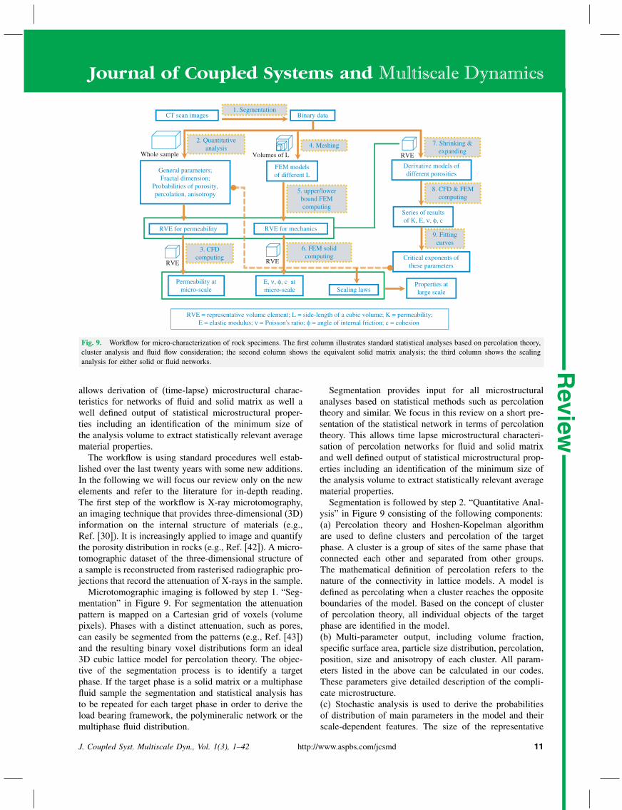
Fig. 9. Workflow for micro-characterization of rock specimens. The first column illustrates standard statistical analyses based on percolation theory,cluster analysis and fluid flow consideration; the second column shows the equivalent solid matrix analysis; the third column shows the scalinganalysis for either solid or fluid networks.

allows derivation of (time-lapse) microstructural charac-teristics for networks of fluid and solid matrix as well awell defined output of statistical microstructural proper-ties including an identification of the minimum size ofthe analysis volume to extract statistically relevant averagematerial properties.The workflow is using standard procedures well estab-

lished over the last twenty years with some new additions.In the following we will focus our review only on the newelements and refer to the literature for in-depth reading.The first step of the workflow is X-ray microtomography,an imaging technique that provides three-dimensional (3D)information on the internal structure of materials (e.g.,Ref. [30]). It is increasingly applied to image and quantifythe porosity distribution in rocks (e.g., Ref. [42]). A micro-tomographic dataset of the three-dimensional structure ofa sample is reconstructed from rasterised radiographic pro-jections that record the attenuation of X-rays in the sample.Microtomographic imaging is followed by step 1. “Seg-

mentation” in Figure 9. For segmentation the attenuationpattern is mapped on a Cartesian grid of voxels (volumepixels). Phases with a distinct attenuation, such as pores,can easily be segmented from the patterns (e.g., Ref. [43])and the resulting binary voxel distributions form an ideal3D cubic lattice model for percolation theory. The objec-tive of the segmentation process is to identify a targetphase. If the target phase is a solid matrix or a multiphasefluid sample the segmentation and statistical analysis hasto be repeated for each target phase in order to derive theload bearing framework, the polymineralic network or themultiphase fluid distribution.

Segmentation provides input for all microstructuralanalyses based on statistical methods such as percolationtheory and similar. We focus in this review on a short pre-sentation of the statistical network in terms of percolationtheory. This allows time lapse microstructural characteri-sation of percolation networks for fluid and solid matrixand well defined output of statistical microstructural prop-erties including an identification of the minimum size ofthe analysis volume to extract statistically relevant averagematerial properties.Segmentation is followed by step 2. “Quantitative Anal-

ysis” in Figure 9 consisting of the following components:(a) Percolation theory and Hoshen-Kopelman algorithmare used to define clusters and percolation of the targetphase. A cluster is a group of sites of the same phase thatconnected each other and separated from other groups.The mathematical definition of percolation refers to thenature of the connectivity in lattice models. A model isdefined as percolating when a cluster reaches the oppositeboundaries of the model. Based on the concept of clusterof percolation theory, all individual objects of the targetphase are identified in the model.(b) Multi-parameter output, including volume fraction,specific surface area, particle size distribution, percolation,position, size and anisotropy of each cluster. All param-eters listed in the above can be calculated in our codes.These parameters give detailed description of the compli-cate microstructure.(c) Stochastic analysis is used to derive the probabilitiesof distribution of main parameters in the model and theirscale-dependent features. The size of the representative



Rev

iew

volume element (RVE) can be determined if the proba-bilities are convergent. RVE’s are here defined as statisti-cally representative volumes containing a sufficiently largeset of microstructure elements such that their influenceon the average macroscopic property (porosity, elasticity,permeability, etc.) has converged. Simulations of proper-ties based on the RVE are deemed to be reliable as theyencapsulate the intrinsic material heterogeneity.

Presently a normal micro-CT dataset is 20483. Volumesof 40963 are now available and it is expected to be 81923 inthe near future. With high performance computation tech-niques of parallelisation and data decomposition, we candeal with extremely large datasets.For the statistical characterisation of the percolation

network computational techniques are used as inputs forhomogenisation of the fluid and solid material properties.If the target phase is a pore space the so characterisedpercolation network lends itself for a computational fluiddynamic computation (step 3. “CFD computing” in Fig. 9)with the purpose of delivering a permeability value of thesample. A variety of numerical methods are used for thisstep such as finite difference, finite element, smooth parti-cle hydrodynamics and Lattice-Boltzmann techniques. Forfinite element analysis standard preprocessing in step 4.“Meshing” of Figure 9 is required.The steps 5 and 6 in Figure 9 rely on computa-

tional homogenisation techniques generalised for geologi-cal systems. They are based on well established conceptsfor multiscale convergence of microstructure in materialsciences�44� with the main difference being that geologicalprocesses need to consider additional multiscale and multi-physics couplings on time scales that are inaccessible tothe laboratory verification. This adaptation to geologicalsystems is mainly enabled through the application of per-colation theory introduced in steps 7–9 of Figure 9.

5.1. Percolation Theory in Real SpaceSince its establishment in mathematical physics in the1950s, percolation theory�45� has been applied to earthscience for investigating various phenomena in heteroge-neous media, including various flow phenomena in porousmedia,�46� transport, reaction, diffusion and mineral pre-cipitation, distribution of earthquakes, and mechanicalproperties.�47� In this section we focus on the application ofpercolation theory combined with X-ray microtomography.Fluid flow through pores and/or cracks in solid media

is one of the most important topics in earth sciences,with important applications to energy industries and min-eral deposits. The prerequisite of fluid flow is the con-nectivity of voids. Percolation theory describes the globalconnectivity of models and thus can be used to anal-yse microtomographic datasets of porous materials. Refer-ence [48] first used the local porosity theory�49� to anal-yse 3D microtomographic data and compared the porespace geometry of different samples quantitatively, where

the local percolation distribution is the probability ofpore-connectivity of sub-volumes. Reference [50] devel-oped a program for the analysis of pore connectivity andanisotropic tortuosity of porous rocks. Reference [51],studied the evolution of porosity and hydraulic diffusivityduring weathering of basalt. Reference [40] extended thelocal porosity theory to consider anisotropic permeabilityin percolating sub-volumes.The key parameter in percolation theory is the percola-

tion threshold, which describes the (minimum) porosity ofa connected network of pores.�45� The percolation thresh-old can be derived from a percolation cluster analysis inwhich a group of face-connected cells forms a cluster.Labelling clusters that belong to a target phase in a seg-mented microtomography dataset is the process wherebyall voxels (i.e., cells) in a cluster are given a unique label.After cluster labelling, each individual structure of the tar-get phase is resolved, including the position, size, and ori-entation. The percolation threshold can then be determinedby analysing percolation in a series of datasets with differ-ent volumes as laid out in the theory review.�2� We reviewhere the first applications of percolation theory. In a firstattempt to analyse realistic natural geometries with perco-lation theory, Ref. [52] studied the geometrical percola-tion threshold of porous media by assuming grains to beoverlapping ellipsoids. The authors found the percolationthreshold to be ranging from 0.06% to 28.5% for differentaspect ratios and ellipsoid sizes.Reference [53] created virtual permeable microstruc-

tural models of hard-core-soft-shell grains and obtaineda percolation threshold of 4% for concrete-like porousmedia. These mathematical models are limited to idealor special structures. Reference [51] collected a suite ofweathered basalt samples with porosities between 3% and30% and found that 9% is the percolation threshold ofthe specific weathered basalt. Reference [54] tested cumu-lates of sea ice single crystals at different temperatures anddetermined percolation thresholds of (4.6± 0.7)%, (9±2)%, and (14±4)% in different directions. For most natu-ral samples, a series of models with different porosity andsimilar structure is not available. Reference [41] proposeda new method for determining the percolation threshold ofnatural structures by generating a virtual series of digitalsamples from a single dataset. By volumetrically shrink-ing or expanding the pore-structure of the static images,a series of models with similar structures but differentporosities are created. The percolation threshold can bedetermined for each individual structure.

5.1.1. Applied Case Study: Critical PercolationPhenomenon in a GraniticShear Zone in Australia

This analysis was applied to assess the role of microporesin the deformation of a granite at the base of the seismo-genic zone in the continental lithosphere.�55� A deformed



Review

granite from Central Australia that has been subject to400–500 �C environment was analysed. The granite is nowexposed to the surface so that the shear zone can be sam-pled and analysed using Synchrotron-based X-ray micro-tomography (Fig. 10). Microtomographic data was used todescribe the porosity distribution across the shear zone andinterpreted in combination with a classical microstructuralstudy of the evolution of the strained rock.The analysis with the percolation theoretical approach

supported three important discoveries:�55�

(1) Porosity evolves with progressive deformation, anddifferent mechanisms contribute to the overall porosity atdifferent stages of the microstructural evolution. In themost deformed rock samples with the finest grain sizes,grain boundary pores, formed by creep cavitation, domi-nate the porosity architecture;(2) the maximum porosity in the centre is close to but justbelow the percolation threshold of 5%;(3) Minerals precipitated in the pores evidence synkine-matic fluid migration and the redistribution of chemicalcomponents on a length scale significantly exceeding thedimensions of pores and minerals (see Fig. 3 in Ref. [56]).

These observations contribute to explaining fluid flow ininterseismic periods at the base of the seismic zone. Atthe highest strains creep cavities self-organise in ductileshear bands, analogues to ductile failure phenomena inmetals and ceramics,�57–59� and promote fluid transfer overdistances significantly larger than individual grain diame-ters. This behaviour can be best modelled using a dam-age mechanics approach, and a suitable formulation willbe reviewed in the constitutive modelling section. In thenext section we will show that detection of the percolation

D01: 2.43

F01: 2.50

F03: 2.62

G04: 2.52

H03: 2.82

J05: 2.82

1 cm

C02: 2.46

B01: 2.45

Fig. 10. A hand specimen of a mylonitic shear zone and the fractaldimension obtained through X-ray CT analysis of micro-cores sub-samples (B01–J05), locations shown in red. The fractal dimension isincreasing towards the centre of the shear zone where the smallest grainsize is observed.

threshold plays an important role in extracting criticalexponents and scaling laws for upscaling.We analyse percolating porosity clusters in the geologi-

cal hand specimen described in Ref. [55]. Figure 10 showsthe specimen together with the locations and labels ofsubsamples scanned by Synchrotron X-ray microtomogra-phy. Note that the hand specimen covers a strain gradientinto a highly deformed shear zone. In the centre of theshear zone, the minerals are much more finely grained thanat the perimeter, which is an effect of deformation. Thefractal dimension d of the pore size distribution in the sub-samples can be calculated from the segmented microtomo-graphic data using percolation cluster analysis. The resultsare listed behind the label in Figure 10. It appears that ahigher fractal dimension exists in the centre than at themargin of the shear zone. According to the energy scalinglaw�60� the dissipated energy of the fragmentation processof a solid is proportional to its volume to the power ofd/3. That implies that the higher the fractal dimension thehigher is the dissipated energy. This result demonstratesthe link between the fractal dimension, energy dissipation,and deformation. Although it is not a surprising result thatthe centre of the shear zone exhibits the highest energydissipation this analysis gives the geologist a quantitativetool to analyse and describe the dissipation. The quantifi-cation of the dissipated power is an important diagnostictool to compare model predictions from constitutive mod-elling with natural samples.Other quantities that are of interest and can be extracted

from microtomographic data analysis are the anisotropy ofpermeability in a sample, which is related to the anisotropyof the geometry of percolating cluster. The anisotropy ofa cluster is described by an orientation tensor.�2,40, 61� Stillmore information can be revealed from the cluster analy-sis, such as how much pore space is connected, whethernon-percolating clusters are oriented or what their spe-cific shapes are. The fractal dimension can also be cal-culated by additional methods showing self-consistent andscale-independent characteristics. mic Additional informa-tion derived from the above rock sample is for instancethe size distribution of pores and the volume percentageof different cluster-sizes (Fig. 11). This analysis reveals abimodal distribution of pore sizes which is again a resultof the dynamic recrystallisation in the centre of the graniticshear zone.

5.2. Renormalisation Using Percolating TheoryRenormalisation is achieved by using the stochastic anal-ysis of the moving window method, and probabili-ties of porosity, percolation and anisotropy are derived.Reference [40] illustrates the use of percolation theoryfor the derivation of RVEs. For better comparison withmathematically constructed reference models a syntheticsandstone sample was selected. The excellent agreementbetween mathematically predicted and numerically esti-mated values, derived by applying the X-ray CT workflow



Rev

iew

0

1

2

3

4

5

1E+0

1E+1

1E+2

1E+3

1E+4

1E+5

1E+6

1E+0 1E+1 1E+2 1E+3 1E+4 1E+5 1E+6 1E+7

Per

cent

age

of p

ores

(%

)

Clu

ster

num

ber

Cluster size (voxel)

Fig. 11. Histogram of cluster size and the volume percentage of dif-ferent cluster-sizes.

on the synthetic sample, gave credence to the technique.In this ideal example of renormalisation, probabilities ofporosity, percolation, isotropy index and elongation indexare all convergent when the sub-volume-size is larger than4003 voxels or 1 mm3. Thus the RVE size of geometry ofpore-structure was determined.The derivation of the critical exponent of correlation

length was investigated in subsequent work using the samesynthetic sample.�41� Probabilities of percolation of dif-ferent sizes and finite-size scaling scheme were used toderive the critical exponent. The critical exponent of corre-lation length was found to be 0.885, which is very close tothe theoretical expected result of 0.88.�45� Combined withother scaling parameters, such as the percolation threshold,crossover length, and the fractal dimension, the scalinglaws of the sample were identified and the permeability atmicroscale was proven to be usable for large scale directly,without rescaling.

5.3. Asymptotic HomogenisationThe asymptotic computational homogenization methodpostulates that through a stepwise increase in microstruc-tural cell size the apparent material property can be derivedasymptotically.�44� In such a method the material prop-erty such as Young’s modulus is found to be consistently

Microstructural cell size

Mat

eria

l Pro

pert

y

Flux BC

Forc

e BC

Uncertainty

CT

-sca

n

Fig. 12. Thermodynamic homogenisation procedure considering combinations of constant thermodynamic force and constant thermodynamic flux.Modified diagram inspired by a plenary lecture by Robert L. Taylor, University of Berkeley, California, on Computational Mechanics Today 2008.

overestimated (stronger) for a displacement boundary con-dition (constant thermodynamic flux) while the prop-erty is consistently underestimated through the choice ofa traction boundary condition (constant thermodynamicforce).�2� The solution of such a boundary value prob-lems delivers a lower bound for a constant force boundarywhile the constant displacement boundary problem givesan upper bound of the work done. When the volume issufficiently large the two bounds converge.�62� Thus themechanical RVE size is identified. The limit theoremawere initially formulated for specific dissipative elasto-plastic systems but they have been shown to be applicableto generalised thermodynamic forces and fluxes.�2,63� Thegeneric computational asymptotic homogenisation proce-dure is illustrated in Figure 12. In the following, applica-tions of asymptotic homogenisation for conservative forceand non-conservative force are given.

5.3.1. Asymptotic Homogenisation forConservative Forces

Since the critical percolation threshold corresponds to ascale-dependent phase-change in the physics of the inves-tigated process, the renormalisation procedure of perco-lation theory allows a robust assessment of fundamentalchanges in material parameters and their scaling relation-ships before and after the critical point. Some parame-ters are changing exponentially when the volume fractionis approaching the percolation threshold. These parame-ters include permeability, elastic modulus, yield stress, andmore.We first consider the simple case of non-conservative

thermodynamic forces, such as the linear elastic responseof microstructures for a carbonate sample from an oilfield with a heterogeneous microstructure is shown inFigures 13 and 14. The classical asymptotic homogenisa-tion procedure of material sciences should be applicableto this class of problems.�44� Note that this considera-tion is not common practice in geosciences. Much sim-pler methods such as the Gassmann equation are thecurrent state of the art in geophysics.�64,65� For sand



Review

Fig. 13. A carbonate sample and the homogenisation of upper and lower bounds of elastic modulus. The bulk porosity of the sample is 26%. Imageresolution is 1.85 micron. Input solid elastic modulus is 50 GPa and Poissons ratio is 0.2.

shale reservoirs Gassmann has proven its value. How-ever, for carbonates, which contain more than 60% ofthe worlds oil reservoirs,�64� one has yet to find a sim-ilarly successful technique. Currently, elastic propertiesused for the detection of these reservoirs through seis-mic methods still use Gassmann formulation�66� in fullacknowledgments that carbonates are notoriously difficultto describe via homogenisation methods. The main prob-lem is the multiscale heterogeneity of carbonates at micro-and macro-level. At micro-level the grain contacts andinclusions cause heterogeneous mm-scale microstrucureand at macro-level vugs and solution cavities yield cm-m scale heterogeneity. We propose here to use the abovedescribed workflow in two different stages. In the first

16

24

32

L=50 L=100L=150 L=200L=250 L=300L=350 L=400L=450 L=500

0.4

0.6

0.8

1

L=50 L=100

0

8Fre

quen

cy (

%)

0

0.2

Pro

babi

lity

of p

erco

latio

n

L=150 L=200L=250 L=300L=350 L=400L=450 L=500

Porosity Porosity

4

5 L=50 L=100 L=150

L=200 L=250 L=300

L=350 L=400 L=450 4

5L=50 L=100 L=150

L=200 L=250 L=300

L=350 L=400 L=450

(a) (b)

1

2

3

Fre

quen

cy (

%)

L=500

1

2

3

Fre

quen

cy (

%)

L=500

0

Isotropy Index

0

0 0.1 0.2 0.3 0.4 0.5 0 0.1 0.2 0.3 0.4 0.5 0.6 0.7 0.8

0 0.1 0.2 0.3 0.4 0.5 0.6 0.7 0.8 0.9 1.0 0 0.1 0.2 0.3 0.4 0.5 0.6 0.7 0.8 0.9 1Elongation Index

(d)(c)

Fig. 14. Probabilities of porosity (a), percolation (b), isotropy index (c) and elongation index (d) of a carbonate sample.

stage we use the micro-CT data analysis to homogenisethe heterogeneity at micro-level and in a second step (notyet performed) we propose to use sonic logs and bore-hole images or similar for an upscaling of the next scaleusing the effective properties derived from the micro-levelas matrix properties. Because of the wavelength of seismicwaves this would be the main scale of interest. For thispurpose we discuss a carbonate sample of a major oil fieldfound through deep ocean drilling and attempt a mm-scalehomogenisation procedure (Fig. 13).Two criteria are used for cropping volumes in the

asymptotic homogenisation procedure: (1) each smallervolume must be a subset of a larger volume; (2) eachcropped volume has the porosity close to the bulk porosity,



Rev

iew

i.e., difference is less than 1.0%. For each cropped model,we use the finite element method to analyse the responseof displacement and pressure loads, respectively. The fol-lowing boundary conditions are given:(1) normal displacement constraint on the surfaces of x=xmin� y = ymin and z= zmin,(2) free surfaces on x = xmax and y = ymax,(3) displacement or pressure load on the surface of z =zmax, where min and max denote two end boundaries in x,y and z directions.

Mathematically, this constraint is equivalent to the uncon-fined compression of a sample with mirror images of thevolume in x, y and z directions. The magnitude of load-ing is small enough to ensure that only elastic deformationoccurs. In our model, only the solid skeleton is consid-ered while pores are void and have no strength. Thus onlyelastic parameters of the solid are necessary as input.Two kinds of meshes are used for these volumes for

finite element computation. Hexahedral elements are usedfor small volumes of side-length < 100 voxels, which areeasy to create and the computing time is acceptable. Tetra-hedral elements are used for large volumes, generally for≥ 100 voxels. This entails extra procedures and manualwork but it can dramatically reduce the computation time.For creating tetrahedral element meshes, we considered thebalance of keeping the precision and the fineness of themesh and reducing the computing time. A typical exampleis shown in Figure 13. For small volumes the oscillationsclearly indicate the limit of validity of the thermodynamicassumption. The lower bound shows stronger oscillationthan upper bound, however, the micro-elastic propertiesappear to converge. For this specific case, the mechanicalRVE size can be determined as 2003 voxels.

5.3.2. Percolation Theory Applied toNon-Conservative Forces

Having identified the micro-mechanical RVE for conser-vative forces we extend the study to problems with dissi-pation. We consider Drucker-Prager plasticity of the rockover a mechanical RVE. In order to conduct cohesion andthe angle of friction of rock samples, two cases of differ-ent pressures are simulated. Using the relationship of y =n tan +c where y and n are the yield stress and nor-mal stress computed from Drucker-Prager plasticity, andc and are cohesion and the angle of internal friction ofthe rock. With the two groups y and n resulting frommodel calculations of the macroscopic model c and canbe deduced. Numerical simulations with at least two dif-ferent pressures are necessary to detect cohesion and theangle of friction of the microstructure.For each case, the stress–strain relationships are com-

puted (Fig. 15). We label von Mises stress and pressure atthe yield point as Sy and Sn in Figure 15. The yield pointof Case 1 is identified as shown in Figure 15(a); the yieldpoint of Case 2 can be arbitrarily selected at the strain of

0

20

40

60

80

0 0.002 0.004 0.006

Str

ess

(MP

a)

Strain

Case 1

Case 2

0

10

20

30

0 10 20 30 40 50

Mis

es s

tres

s (M

Pa)

Pressure (MPa)

Case 1 - yield

Case 2 - yield

y = 0.133 n + 21.04

(a)

(b)

Fig. 15. Plasticity analysis: (a) Stress–strain relationships of twocases; (b) von Mises stress and pressure relationships of two cases andthe fitting of cohesion and the angle of friction.

0.1% or 0.2%. For Case 1, the relationship between vonMises stress and pressure is linear before yielding occurs;both von Mises stress and pressure are constant after yield-ing. For Case 2, von Mises stress and pressure show twolinear relationships before and after yielding. The lineartrend after yielding is connected to the point after yield-ing of Case 1. It implies that any two points after yieldingof Case 1 and Case 2 will give the same result of cohe-sion and the angle of friction. A fitted line is shown inFigure 15(b). The slope and the intercept are 0.133 and21.04, respectively. Thus the cohesion is 22.04 MPa andthe angle of friction is 7.8�.

Shrinking/expanding algorithms�41� are used to createa series of derivative models with different volume frac-tions. Then the derivative models close to the percola-tion threshold are used to simulate the deformation andyielding. With a series of results of yield stress of mod-els, it is possible to fit the critical exponent of yieldstress. Figure 16(a) shows five examples of stress–strainrelationships of derivative models close to the percola-tion threshold. Different derivative model have differentresponses, from elastic-perfect plasticity to plastic hard-ening behaviour, and the yield stress is increasing withhigher volume fraction of solids. Figure 16(b) shows theexample of fitting the critical exponent of yield stress. The



Review

0.02

0.2

0.03 0.3

Yie

ld s

tres

s

|P - Pc|

y = 26.63 (ppc)2.3

0.0

0.5

1.0

1.5

2.0

0.E+00 2.E-05 4.E-05 6.E-05 8.E-05 1.E-04

Str

ess

(MP

a)

Strain

P - Pc = 0.1519 P - Pc = 0.1278 P - Pc = 0.0937 P - Pc = 0.0775 P - Pc = 0.0632

(a)

(b)

Fig. 16. Plastic response of derivative models close to (a) percolationthreshold; (b) the fitting of the critical exponent of yield stress.

best fit of the critical exponent of yield stress is 2.3, whichis close to the theoretical result.

5.4. Example Numerical Upscalingfor Westerly Granite

This section summarises an example for numerical upscal-ing using a classical benchmark material of the rockmechanics community: Westerly granite.�67–70� In this casestudy, we investigated the magnitude and longevity ofthermal-elastic internal stresses in granite induced by slowburial over geological time scales.�71�

It is well known that heating and lithostatic loading ofrock lead to high internal stresses.�72,73� The reason liesin the mismatch and anisotropy of the thermal-expansionand elasticity tensors of the constituent minerals. Thesematerial properties may differ by as much as one orderof magnitude, and consequently, heating of rocks by sev-eral hundred degrees and compression induce internal con-tact stresses of order 100 MPa. Thermal-elastic internalstresses have mainly been examined in the context of brit-tle rocks, where they generate micro-cracks.�68� Micro-cracks affect rock properties such as elasticity, strength,thermal conductivity, and permeability and thus attractedresearch efforts in the fields of mining, drilling, nuclearwaste disposal and reservoir stimulation.�68,69, 74� Beyondconfining pressures of about 100 MPa, reached at ca. 3to 4 km depth in the continental crust, micro-cracking islargely suppressed.�75� At greater depths, the continental

crust of the earth assumes temperatures > 50% of themelting temperature of its main constituents (quartz andfeldspar). At these temperatures (ca. 300 �C for quartz,usually attained at a depth of ca. 10 km), rocks begin todeform by crystal-plastic, ductile deformation processessuch as dislocation and diffusion creep (e.g., Ref. [76]). Itis often assumed that these creep processes relax thermal-elastic internal stresses quickly, and hence they are usu-ally disregarded in deformation processes in the ductilecrust.�77,78�

Since ductile creep is a slow, time-dependent process,we decided to examine how large thermal-elastic inter-nal stresses can become and how long they are sustainedwhen granite is buried slowly and deeply in the conti-nental crust. Because of the low burial rates and largerelaxation times associated with creep processes, thesequestions cannot be addressed by laboratory experiments.Hence, we resorted to combining physical heating exper-iments on Westerly granite observed with time-series 3DSynchrotron computed micro-tomography and numericalupscaling. The physical experiments were used to deter-mine the effective material properties of the mineral con-stituents of our Westerly granite sample. Empirical 2Dnumerical inversion models mimicking the physical exper-iments achieved this goal. Finally, the calibrated numericalmodels were extended to simulating the loading condi-tions and ductile creep encountered during the slow burialof granite in nature. This workflow is summarised in thefollowing.

5.4.1. Physical Heating Experiment: Time Scale ofHours, �T of 200 �C, and �p of 0 MPa

A mm-scale cylindrical sample of Westerly granite wasslowly heated over an interval of 200 �C from room tem-perature and at ambient pressure (see Fig. 17(a)). The slowexpansion of the sample and the formation of micro-crackswere monitored at a resolution of 1.3-micron voxel edgelength with a tomograph. Bulk radial expansion and crackstatistics were employed as constraints for 2D numeri-cal calibration experiments, which served to determine thematerial properties of the mineral constituents.

5.4.2. 2D Numerical Calibration Experiment: TimeScale of Hours, �T of 200 �C, and �p of 0 MPa

Knowledge of the thermal-expansion and elastic prop-erties of the individual mineral constituents of graniteis paramount for estimating thermal-elastic stresses atthe grain scale. These properties change with increas-ing temperature and were estimated with Gibbs energyminimisation�79� or taken from laboratory experiments.�80�

These methods presume that the minerals are intact. Ourtomograms showed that our sample contained a signif-icant amount of pre-existing intracrystalline pores andcracks (see Fig. 17(a)), resulting in a noticeable reductionof the undamaged elastic moduli and thermal-expansion



Rev

iew

Fig. 17. (a) This image shows the tomogram considered in our numerical experiments. It is a quarter of a horizontal cross-section through thesample cylinder prior to heating. Sample radius is ∼ 1.2 mm. The inset in (b) provides a key to the minerals observed in the image (Qz = quartz,Mc=microcline, Pl= plagioclase, Bt= biotite). Note the significant amount of pre-existing damage (regions with black or dark grey colours), bothalong grain boundaries and within grains. Plagioclase (for example, grain in the lower left corner of the tomogram) exhibits a particularly largeamount of intracrystalline pores. (b) 2D contour plot of maximum differential stress (colour scale in MPa) predicted for slow burial with a typicalgeological velocity of 1 cm/a along a simplified equilibrium geotherm corresponding to a surface heat flow of 70 mW m−2. This stress state isreached at a temperature of 350 �C and a confining pressure of ∼ 400 MPa.

coefficients. We used an empirical method for invert-ing effective material properties, as described in thefollowing.A horizontal 2D cross-section through the centre of

the physical sample was digitised, thus reproducing theactual microstructure of the rock and approximating plane-strain conditions (see inset of Fig. 17(b)). For simplicity,only a quarter of the circular cross-section was mod-elled. The model grains were simulated as isotropic, homo-geneous, linear-elastic materials. However, their surfaceswere modelled with contact mechanics, allowing for dis-sipative grain-boundary cracking. An elastoplastic dam-age law was employed, constrained by experimental dataon the tensile yield strength of Westerly granite.�81� andatomic binding models.�82� The thermal expansion coef-ficient of quartz is the most important factor for theexpansion behaviour of granite.�78� Thus, and for compu-tational convenience, we regarded it as tuning parameter.The thermal expansivity of quartz was reduced linearlyacross the relevant temperature range while the expan-sion coefficients of the remaining minerals were decreasedproportionally to quartz. We used the bulk radial strainobserved in the physical experiment as main constraint(Fig. 18).The quality of the fitted calibration model was tested

against independent physical experiments on the samematerial conducted on much larger (cm-scale) samples.�74�

Our calibrated model predicted the temperature evolutionof the upscaled bulk thermal expansivity of Westerly gran-ite very well (Fig. 19). In addition, the modelled grain-boundary crack behaviour matched independent laboratoryexperiments well.�69,83�

5.4.3. Upscaled 2D Numerical Burial Experiment:Time Scale of Millions of Years, �T of500 �C, and �p of 670 MPa

In the final step, the calibrated 2D model was usedto simulate grain-scale thermal-elastic stresses in gran-ite under loading conditions characteristic of geologicalburial. Therefore, the time scale of the experiment wasupscaled from hours to millions of years. The burial modelwas augmented in two ways: (a) a time-dependent litho-static pressure was applied to the model surface, and (b)in addition to elasticity and grain-boundary damage, therheology of the minerals included rate-dependent plastic

Fig. 18. Comparison of mean radial strain as a function of tempera-ture measured in the physical experiment (error bars denote resolutionerror of the tomograms) and predicted by the 2D numerical calibrationexperiment.



Review

Fig. 19. Linear thermal expansivities as reported by Ref. [74] versusmean linear expansivity predicted by our calibration experiment. Theterms rift, grain, and hardway are quarrying terms and denote planesof easiest, intermediate, and hardest splitting of the rock. Experimentallinear expansivities were measured normal to these planes.

creep from fairly well established laboratory experiments(e.g., Refs. [84, 85]).The results of this case study suggest that thermal-

elastic stresses can reach magnitudes well in excessof 100 MPa with lifetimes of order millions of years,even at temperatures where ductile relaxation occurs seeFigure 17(b). We thus identified an important potentialsource for upward-cascading of thermal-mechanical insta-bilities. This particular upscaling problem highlights theimportance of the relative diffusive time and length scalesinvolved in rock deformation problems, here those of ther-mal and stress diffusion.

6. MICROSTRUCTURALLY ENRICHEDCONTINUUM FOR GENERALISED RATEDEPENDENT SOLIDS

The above described microstructure homogenization work-flow provides the basic framework for upscaling of prop-erties of materials with microstructures based on wellestablished theories. We have shown how the quantifi-cation of the scale dependence of uncertainties of thesematerial properties can be derived from thermodynamicextrema of minimum and maximum entropy produc-tion. However, the complementary approach of constitu-tive modelling is less straight forward. This is becauseclassical continuum models do not have a length scaleand therefore cannot accommodate microstructure.�86� Thisposes a significant problem as the classical constitutivelaws cannot be used without modifications, and the ques-tion arises what are the fundamental material propertiesto be homogenised by the workflow and how do theyincorporate the microstructure information. As a prerequi-site for using thermodynamic extrema for deriving mate-rial properties, we need to ideally close the loop using

a constitutive approach that is also primarily based onthermodynamics.The classical constitutive modelling approach from plas-

ticity theory, which is excellent for deriving constitutivemodels from controlled laboratory experiments, thereforeneeds to be extended to being closer to basic thermody-namics and the underlying physics. In classical plasticity,constitutive laws are for instance derived by postulating anelasticity law, a yield function and a plastic flow rule (seeFig. 20). The consistency with the 2nd law of thermody-namics is implied either through the orthogonality principleor verified thereafter to validate the resulting incrementalrelationships. This approach provides an implicit or indirectconsideration of thermodynamic constraints.Over the recent years, an alternative approach has

matured, which uses a direct consideration of the ther-modynamic principles.�87–91� We have already brieflydiscussed the concepts in the theory review.�2� In the fol-lowing, the key ideas are summarised in further detail. Webegin with the local, weak form because the integral ofthe strong form already encapsulates the Min/Max theo-rema of entropy production that arises because of the pathdependence. Consider the first law of thermodynamics:

dU = �W tot +�Q (3)

where dU is the differential internal energy, �W tot is theincrement of work done and �Q the heat supply to the sys-tem. In full analogy to the comment on path dependencein the strong form (Ref. [2]), we emphasise here that theincrements of work and heat are not complete differen-tials while the internal energy is a proper differential. Thesecond law of thermodynamics states that:

�Q ≤ TdStot (4)

Note that the total entropy differential dStot = �Srev +�Sir is a complete differential while the irreversible entropy�Sir and the entropy flux on the boundaries �Srev areincomplete differentials. Since �Srev ≡ �Q/T , the secondlaw can be rewritten as Sir ≥ 0. Likewise, by using thedefinition of the internal energy, we can relegate the pathdependence to the irreversible entropy differential �Siror its time derivative, the irreversible entropy productionSir . This is an important constraint for the uncertainty ofthe system expressed in the incomplete differential Sir .Another important finding is that, in the non-isothermalcase, we have to track the total entropy production in anon-isothermal system.

U ≡��i�+TStot

U = ��i�+ T Stot +T Sir

(5)

Substituting the internal energy in Eq. (3), we obtain theclassical equation for the rate of work done in the system:

W tot = ��i�+StotT +T Sir (6)

where the independent state variables �i may havetensorial values. The total work rate W tot = W cons+ W diss



Rev

iew

Elasticity Yield function

Max. dissip. Flow rule

2nd law

Incremental relationship

Helmholtz f. Dissip. function

Flow rule

Incremental relationship

Legendre Transform (2nd law)

Yield function

Consistency Plasticity Approach Direct Thermodynamic Approach

Fig. 20. The consistency plasticity approach postulates elasticity, yield and flow rule independently and verifies the consistency with the second lawindirectly either through Ziegler’s orthogonality principles (maximum dissipation) or through independent verifications. The direct thermodynamicapproach postulates the thermodynamic energy potentials (Helmholtz free energy and dissipation potential) and derives the yield function, elasticitylaw and flow rule through the Legendre transform.

is composed of a recoverable and a dissipative termdescribed by the rate of Helmholtz free energy plus thework associated to the entropy production. The dissipatedwork rate W diss is again composed of a work rate related tothe net entropy change of the system through fluxes on itsboundaries plus the internal irreversible entropy productioninside the volume. In a classical mechanical analysis, it isoften assumed that the process is isothermal, hence T =constant and the work term corresponding to the changeof the total entropy of the system StotT = 0. In eithercase, isothermal or non-isothermal, we are left with a com-plete thermodynamic description where the total work rateW tot can be described by two potential functions, the freeenergy production plus the dissipation potential.This opens the way for direct consideration of ther-

modynamic constraints leading to the proposed develop-ment of constitutive models for microstructurally enrichedcontinua. The procedure originally suggested for rate-independent materials�90,91� is as follows: first, postulatea Helmholtz free energy function ��i�

; second, postulatean internal source of dissipation ��i��i�

= Sir (note that inaddition to the dependence on the state variables �i thedissipation function can depend on the rate of change ofinternal variables �i); third, deduce the yield function andthereby implicitly the elasticity law, hardening rule andflow law.We first assume the dissipative potential ��i��i�

to berate-independent, so homogeneous to first order in theinternal variables �i. We can use Euler’s Theorem andwrite the dissipation:

��i��i�= ��i��i�

��i

�i (7)

where the dissipation is the product of a stress qd =��i��i�

/��i (sometimes called generalised dissipativestress) and a generalised strain rate �i. In the same waywe identify the fraction of the rate of work done (released)for the dissipation by the Helmholtz free energy as:

��i�= ��i�

��i

�i (8)

where ��i�/��i is identified as the generalised stress and

�i is the generalised strain rate. We note that there is nodissipative power without commensurate rate of release ofHelmholtz free energy:

��i�

��i

�i =��i�

��i

�i (9)

for every �i �= 0. This is also known as Ziegler’s orthog-onality or the maximum entropy production principle. Asproposed by Ref. [90], the roles of the incremental changeof Helmholtz free energy ��i�

/��i (generalised stress)and the rate of change of the state variable �i (generalisedstrain rate) can be interchanged by a Legendre Transformto give the yield function y��i�

:

�y�i= ��i�

��i

�i−��i�

��i

�i = 0 (10)

where � is a non-negative multiplier. Taking the timederivative of the yield function, we obtain the flow rule:

�i = ��y��i�

�qd(11)

In consistency plasticity the constant � is classicallyevaluated through the consistency and loading condition



Review

y = �y = 0, ensuring that the stresses do not exceed theyield surface. Later on, we will describe an alternativeformulation where stresses are allowed to exceed the ini-tial yield surface. This formulation is called the overstressplasticity formulation.Both formulations enable so-called enriched continuum

formulations with the direct consideration of dissipativeprocesses and their energy feedbacks. Such feedbacksmay lead to localisation of deformation into narrow shearbands with a small but finite width. Other than describ-ing the homogenisation of the material microstructure, theenriched continuum model embeds a characteristic mate-rial length scale that acts like a localisation limiter. Thematerial length scale is, in the above described formula-tion, directly based on the consideration of the internalenergy interactions and dissipation through the microstruc-ture. An example was given in the theory review�2� where,for instance, the energy incorporated in rolling and slid-ing mechanisms of granular media reveals that shear bandsare formed due to the rolling component, with their thick-ness varying with the rolling resistance. Much like in thecase of the partial melts (see Fig. 5), where a length scaleemerges out of hydro-mechanical diffusion, a new diffu-sive mechanical length scale emerges. In classical enrichedcontinuum formulations, the shear band width can beshown to depend on the size of the individual grains,which affects the momentum diffusion. We have discussedthat the energy considerations also reveal a rate effect notdescribed by the classical Cosserat theories. Because therates of processes play an important role in earth science,we will focus on the presentation of the various effects ofrate sensitivity on localisation phenomena in the following.

7. COMBINING SOLID AND FLUIDDYNAMICS FOR GEOMECHANICS

In order to introduce rate sensitivity, we review the dif-ferent solid-mechanical and fluid-dynamic approaches. Wewill summarise two theories describing this transition,consistency plasticity and overstress plasticity. We alsohighlight their relationship and introduce the fundamentalthermodynamically inspired strain-rate decomposition.

7.1. Definition of a Solid versus a Fluid RVEFirst, we define the fundamental difference between a solidand a fluid in terms of the overall mechanical behaviourof a RVE. In the microstructure homogenisation workflow,we have discussed the statistical description of distributednetworks, percolating or not, of an arbitrary volume ofrock. We can use percolation criteria to define solid andfluid behaviour if we consider the material network tobe made of force chains �86,92� that can be pictured assmall solid connector rods (hereafter called skeleton) inone subvolume of the RVE. At the level of the RVE, asolid is then defined by the case where percolation of theforce chains through the considered volume occurs, i.e.,

the force chains are connected from one end of the volumeto the other, and the force chain network can support anapplied stress. When the force chains on the level of theRVE are not connected (no percolation), and the materialdefining the force chains (solid skeleton) is unable to sup-port an applied stress. The material must react to this stressby flow and is, at the scale of the RVE, called a fluid.A solid may turn into a fluid through the application of aload by breakage of the force chains.In order to describe this difference in mathematical

terms, we use the formulation of Love�93� of an effectivestress tensor of the RVE ′

ij acting on a RVE of a�54�

having a sub-skeleton of radius R, and sharing the forcesacross the set N of the contacts:

′ij ≈

1VRVE

∑c∈N

lci fcj (12)

where VRVE is the volume of the RVE, lci ≈ R is the vec-tor connecting the centres of each two contact skeletonmaterials and f c

j the force acting on the contact.We use the Terzaghi relation�2� of the effective stress

′ij = ′

ij and the total stress tensor ij

ij = ′ij +bpf �ij (13)

where pf is the fluid pressure, �ij Kronecker’s delta and bBiot’s coefficient.For convenience we describe the problem by the strain

rate tensor �ij through the velocity field of the solid skele-ton V

�s�k , which is related to the fluid phase velocity

through the consistency relationship.�94�

�ij =12

(�V

�s�i

�xj+ �V

�s�j

�xi

)(14)

In Eq. (41) of Ref. [2] we have introduced the additivestrain rate decomposition of poromechanics. This followsdirectly from the generalised decomposition of the totalwork rate by the rate of Helmholtz free energy and thedissipation.

�ij = �eij + �pij (15)

In Eq. (1) of the theory review,�2� we have alsointroduced the generalised incremental relationship ′

ij =C

epijkl�kl where C

epijkl is the elasto-plastic compliance modu-

lus.Assuming a smooth function of the effective stress, tem-

perature T , and additional internal variables �k, we canwrite the constitutive behaviour of the material as:

�pij = f � ′

ij � T � �k� (16)

Further assuming, without loss of generality, that thedeformation is isothermal at a temperature T0 and atmicrostructural steady-state, �k = �0

k , a Taylor expansionof Eq. (16) around the effective yield stress ′

Y yields:

��pij = f ′ ·� ′

ij +∑m≥2

f �m� ·� ′mij (17)



Rev

iew

where ��pij = �

pij − �

pY , �ij = ′

ij − Y and f �m� =�1/m!��dmf � ′

ij � T0� �0k��/d

′mij � ′

ij= ′Y.

7.2. Solid-Fluid Overstress Plasticity versusSolid Consistency Plasticity

The leading order of the linear expansion of Eq. (17) leadsto the classical consistency plasticity formulation:

��pij = f ′� ′

ij � T0� �0k��

′ij (18)

where stresses cannot exceed the yield surface. Conse-quently, all the evolution parameters such as plastic hard-ening and softening are tied to an evolution of the yieldsurface and thus an evolution of the elasto-plastic modu-lus C

epijkl. The latter is commonly derived from laboratory

experiments and not from considerations of the physicaldissipation mechanisms.By considering the higher order terms of Eq. (17), the

stress can exceed the yield surface, and the description ofthe physics of the dissipation processes can be captured.This is also known as overstress plasticity�95� where ij >Y , �

′ij is not an increment any more but it represents the

overstress ij = ij −Y . This approach allows departurefrom the theory of solid mechanics: areas that exceed theyield stress are deforming in a manner defined by classicalfluid dynamics.Near the yield stress the two approaches are identical.

However, the important difference is that after yielding theconsistency plasticity approach lumps the non-linearitiesof the material response into the hardening modulus,whereas in overstress plasticity the stress–strain incrementresponse is directly implemented in rate form. Classicalsolid mechanics deals with the fluid-like response afteryield as if it were a solid (consistency plasticity) whilein overstress plasticity a dual material behaviour can beconsidered: solid before yield and fluid after yield.

8. SELECTED APPLICATION TOPROBLEMS IN EARTH SCIENCES

8.1. Compaction Bands: HM CouplingWe start with a discussion of the possible effects of fluiddynamics properties of materials without considerationof an enriched continuum model to illustrate the impor-tant effect of rate dependence in Geology. For simplicity,we only consider hydromechanical coupling and inves-tigate whether rate effects of this coupling can lead tolocalisation phenomena. We also investigate whether acharacteristic length scale related to the spacing of theselocalisation bands emerges. We ignore the energetic pro-cesses within the localisation band and do not wish tosolve for the width of the localisation band itself. We havepresented in Ref. [2] compaction bands in sedimentaryrocks, which can be explained by classical constitutive the-ories. The solution presented here elaborates on a possiblealternative model (Fig. 5), where the same observationscan be derived from fluid-dynamic rate effects alone.

8.1.1. Bifurcation CriterionSince compaction bands (CBs) are caused primarily bymaterial non-linearities, current models for mechanicalcompaction focus on the behaviour of the solid matrix.Common mechanical driving forces of compaction includegrain breakage,�96� bond breakage,�97� pore collapse andpressure solution�98–101� under a compressive loading.A frequently used criterion for the formation of CBs as anonlinear response (bifurcation) of the skeleton to mechan-ical loading was given by Ref. [102], as an extension of thebifurcation theory used by Ref. [103]. A rate-independentelasto-plastic material, obeying a standard stress–strainincremental response of ′

ij = Cepijkl�kl, would according to

this criterion show material bifurcations in the form oflocalised deformation if the determinant of the acoustictensor (Ljk = niC

epijklnl, ni being the unit vector normal

to the localisation band) is zero. This provides non-trivialsolutions to the eigenvalue problem Ljkuk = 0, uk beingthe tensor’s eigenvectors.�102,104�

Through this criterion, areas of shear-dominated locali-sation (shear bands) and volumetric-dominated localisation(compaction or dilation bands) are identified, as functionsof the loading conditions and the material parameters(Fig. 21). Since this criterion provides the conditions forthe onset of a single localisation band, recently Ref. [105]extended this continuous bifurcation theory�103� to discon-tinuous bifurcation, in order to account for the formationof a discrete, periodic set of compaction bands.The response of a saturated porous medium to mechan-

ical loading entails expulsion of the fluid from the porousmatrix, controlled by its hydraulic diffusivity. Hence, whenthe aforementioned bifurcation criterion is extended to asaturated elasto-plastic material, it provides the necessaryhydromechanical conditions in 2D loading for periodicdilating and contracting instabilities, either in the formof layered strips or checkerboard cells (Vardoulakis�106�

Fig. 21. Yield envelope in generalised stress space p′–q. This studyfocuses on the area of compactions bands and uses the concept of over-stress for loading paths exceeding the yield stress. Insets: failure modesfor shear and compaction bands. Reprinted with permission from [109],J. Fortin, et al., J. Geophys. Res. 111, B10203 (2006). © 2006.



Review

and Vardoulakis and Sulem�107� Figs. 5.7.1 and 5.7.2).These conditions include, apart from the mechanical prop-erties expressed through the acoustic tensor, the hydraulicparameters of the problem (viscous drag coefficient orhydraulic diffusivity), providing a hydromechanical cri-terion (see Ref. [107], Eqs. (5.7.47)–(5.7.49)) as anextension of the eigenvalue problem related to the acoustictensor. The new, hydromechanical problem consists of theeigenvalue problem Aijuj = 0, where Aij is an augmentedtensor including the acoustic tensor Lij and the hydrome-chanical properties, whereas the eigenvector uj includesthe pore pressure.When applied to simple uniaxial compression of a satu-

rated elasto-plastic material, this method reveals that lay-ered instabilities, emerging in the softening domain of the–�-curve of the material, correspond to a regime wherepore fluid pressure obeys a backward-in-time diffusionequation (see Ref. [107], Section 5.8.2). Backward diffu-sion is known to be a mathematically ill-posed problem,which is usually regularised by resorting to viscous and/orgradient considerations.�108�

8.1.2. Failure PatternIt is well known from biaxial and triaxial experimentsthat shear bands are pairs of inclined localisation bands,appearing in the shear band area of Figure 21 and dippingat Arthur-Vardoulakis angle�110,111� as defined in Eq. (6) ofthe theory review.�2� When loaded in the compaction bandarea of Figure 21, CBs will form in an almost horizontaldirection (perpendicular to the maximum principal stress,here set to the axial stress ′

zz), as denoted in the insetof Figure 21 (see for experimental evidence Baxevaniset al.�104� Fortin et al.�109� Oka et al.�112�). Thus, althoughdeviatoric stresses are required to cause pure compaction,the failure mode involves negligible shear deformation, asmeasured by Ref. [112].We may therefore calculate the incremental mechanical

dissipation for this failure pattern,

�Wp = ′ij��ij (19)

to deduce that it is a manifestation of volumetric (and,more specifically, of axial) deformation since �Wp ≈ ′zz��zz. These considerations indicate that the basic

physics of failure in horizontal compaction bands couldbe approximated by a simple 1D model of uniaxialcompression.

8.1.3. Model FormulationIn order to cast these concepts into a simple mathemati-cal model, we consider an infinite slab of height 2H con-sisting of a fluid-saturated, porous geomaterial subjectedto uniaxial compression. We define the stress incrementabove the initial compressive yield stress ′

Y needed tocause the first emergence of CBs as the overstress � ′

zz = ′zz − ′

Y , where � ′zz� > � ′

Y � (see the branch B–C of the

overstress definition in the triaxial space in Fig. 21). Inthis framework, we ascribe a viscoplastic response to thesolid skeleton, given in the lines of the overstress plasticitypresented by Ref. [95]. If CBs form at zero or negligibleoverstress, the mode of deformation is interpreted as brit-tle failure. On the other hand, if the overstress admits anonzero value, CBs are formed in the ductile (cataclasticflow) regime. For further simplification, compressibility offluid and solid skeleton and inertia are neglected. Com-pressive fields (stresses and strain rates) are negative inthis study.

8.1.4. Stress EquilibriumStress equilibrium in the z-direction, combined withTerzaghi’s effective stress ′

zz = zz + p (p > 0 whereas ′zz�zz < 0), provides

� ′zz

�z= �p

�z(20)

The volumetric strain rate always has the same sign as ′zz

(to satisfy the second law of thermodynamics).

8.1.5. Mass Balance ConsiderationsIn a porous medium, we define the partial stresses �1 =�1−n��s and �2 = n�f of the solid and fluid phase, respec-tively, n is the porosity, and �s and �f denote the densitiesof the solid skeleton and the fluid, respectively.In the 1D setting considered the mass balance equations

for each of the phases (refer to Eqs. (9) and (10) in the the-ory review�2�) reduce to the following expressions, whenincompressible solid and fluid are considered (i.e., when�s = const� and �f = const�):

−�n

�t− �nvsz

�z+ �vsz

�z= 0 (21)

�n

�t+ �nvfz

�z= 0 (22)

where viz, i = s� f the partial velocities of the solid andfluid in the z-direction. By adding them we obtain the massbalance equation of the mixture:

�n�vfz −vsz�

�z+ �vsz

�z= 0 (23)

We accept Darcy’s law (Eq. (14)) in the theory review�2�

for the Gersevanov filter velocity n�vfz − vsz�, neglectinghigher order terms,

n�vfz −vsz�=− k�f

�p

�z(24)

and define �vsz/�z= �zz = �v, to get,�107�

k�f

�2p

�z2= �v (25)



Rev

iew

where p is pore pressure, �v the (compressive) volumetricstrain rate, �f the viscosity of the fluid (in Pa · s), and kthe permeability, assumed constant in this study as com-monly done in consolidation theory.�107�

The assumption of constant permeability is adopted heresince this work is limited to the study of the failure pat-tern (onset of failure) rather than the post-failure behaviourof the system. In the general case where permeability,being primarily a function of the porosity, varies in space,Eq. (25) reads:

k�f

�2p

�z2+ 1

�f

�k�z�

�z

�p

�z= �v (26)

Hence, the assumption of constant permeability consideredin this study (Eq. (25)) implies that CBs emerge in areas ofextremum (minimum or maximum) values of permeability,where �k�z�/�z= 0 holds.

8.1.6. Fluid-Dynamic Instabilities ThroughRate-Dependent Material

For the 1D formulation we assume that the solid mechan-ical problem is solved, and the orientation of our1-coordinate system is selected according to the elasto-plastic characteristics for a potential solid-mechanicalcompaction band following the approach of Ref. [102].Having identified the potential solid-mechanical frame-work we can, with the overstress formulation, neglect therole of elasto-plasticity and focus on the fluid dynamicsolution. This analysis allows us to investigate whetherthrough the consideration of a viscoplastic branch newsolutions can emerge, which through the consideration ofthe factor time, allow fluid dynamic instabilities to occur atlower (over)stresses than predicted by the solid-mechanicalsolution. Therefore, we accept rate-dependent (viscous)regularization, by correlating the plastic volumetric strainrate to the overstress through a general viscoplastic powerlaw of the form�113�

�v = �

[� ′

zz

ref

]m

(27)

where � is the creep parameter (in s−1) and ref a referencestress-like quantity, the loading strain rate at the boundarywhere loading � ′

n is applied, is

�n = �

[� ′

n

ref

]m

(28)

If we accept ref as the applied overstress at the bound-ary, � ′

n, then �= �n and the constitutive model could bewritten as

�v = �n

[� ′

zz

� ′n

]m

(29)

where � ′n and �n are reference quantities for the over-

stress and strain rate at which rate dependent behaviour is

validated, here set equal to their values at the boundary,ensuring clarity in the mathematical treatment.Note that the effect of poroelasticity was neglected in

this study, in order to emphasise the conditions for theappearance of spatially periodic failure patterns that canpotentially emerge in the fluid dynamic regime. We haveshown in Figure 5 an example where a fluid dynamiclength scale known as the compaction length may be inter-preted as a criterion for periodic instabilities. This wouldallow a much richer solution space where upon neglect ofthe rate dependence solid mechanical compaction bandsemerge, while for the consideration of rate dependenceboth solid and fluid dynamic instabilities are possible.Reference [113] calibrated the rate-dependency equa-

tion Eq. (27) through isotropic compression data, atvarious strain rates. They deduced that the creep parame-ter � should incorporate the void ratio e, following � =�0/1+ e, and that the rate sensitivity exponent m shouldbe correlated with the slopes of the virgin compressionand recompression curves. Based on this definition, wemay obtain that m > 1�5 for mudstones,�112� m ∼ 10 forporous sandstones�113� and m∼ 100 for kaolinite clay.�114�

Although phenomenologically introduced, we need to notethat the assumed rate-dependency reflects the importanceof the textural composition and mineralogy of the earthmaterials, arising through the presence of even the small-est clay fractions, as well as micro-mechanical processeslike grain angularities inducing rotations and wear, grainbreakage, bond breakage, pore collapse and pressure solu-tion at soft rocks. When upscaled, these micromechanicalproperties yield the necessary rate effects to regularise theproblem.�115,116�

8.1.7. Mathematical ConsiderationsBy combining Eqs. (25), (20), (29) and assuming that ourmaterial is homogeneous and isotropic (hence ′

Y is thesame across the height of the specimen), we obtain thedimensionless effective-stress equation:

d2 ′

dz�2− � ′m = 0 (30)

where z� = zH, ′ = � ′

zz/�′n and

� = �n�f

k�′n

H 2 (31)

8.1.8. Hydraulic Diffusion in the Plasticity RegimeThe parameter � involves the ratio of the characteristicrates of the problem at hand, namely the loading rate(strain rate �n) over the diffusion rate of the pore fluidwithin the specimen of height H when subjected to load-ing � ′

n. The diffusion rate is given as the inverse of thecharacteristic diffusion time

tD = �fH2

k�′n

(32)



Review

Note that the rate t−1D is indeed the ratio of the mod-

ified, poro-plastic hydraulic diffusivity of the mediumcV = k�

′n/�f (in absolute accordance with the classical

poro-elastic expression cV = kK/�f , K being the bulkmodulus of the specimen) over the height H over whichthe load is applied.This modification of the hydraulic diffusivity means that

the hydraulic diffusion time (32) is not a material property(as in classical poro-elasticity), but is mainly controlled bythe applied overstress. For example, in a fluid saturated(�f = 10−3 Pa · s), laboratory experiment (H = 0�1 m, astypical for laboratory specimen), a permeable (k = 10−12

m2) sample would have a very small diffusion time (tD ∼10−2 sec) for large overstresses, of the order of the bulkmodulus (� ′

n = 1 GPa), whereas the same sample wouldhave a very large diffusion time (tD ∼ 102 sec) for smallovertstresses (� ′

n = 100 kPa).Hence even for high permeability values, such as

1 Darcy, and for realistic laboratory conditions where usu-ally the applied overstress does not exceed 1 MPa, thehydrodynamic control turns the problem considered aselastodynamic instability (expressed through the acoustictensor’s eigenvalue problem) into a creeping flow prob-lem controlled by the dissipative properties and time scalesdefined above. In the present context, this transition isexpressed through the dimensionless parameter � (Eq.(31)). When � 1 the specimen is loaded in the elasto-dynamic domain, since the loading rate is lower than thediffusion rate and the specimen has the time to diffuseaway any pressure variations induced by the loading con-ditions. At the other extreme, in the creeping flow regimewhere � � 1, the loading rate is faster than the diffusionrate, pore pressure variations cannot be diffused away andoverpressure can be produced in the specimen leading tohydro- mechanically induced failure in the form of CBs.

8.1.9. Analytical SolutionThe solution of Eq. (30) depends on the value of therate sensitivity coefficient m. For all m > 1 (strong rate-dependency), the solution for ′ is non-trivial, present-ing singularities, as common for this class of equations(see Appendix A of Ref. [117] and literature therein forthe uniqueness and characterisation criterion of diffusion-reaction/absorption equations). For integer values of m <

4 this equation admits closed form solutions. For thesake of mathematical simplicity we focus in this textonly on the relevant solutions producing CBs for strongrate-dependence, under drained loading conditions andchoose without loss of generality a power law exponentof m= 3 and drained boundary conditions ( ′�1�= 1 andd ′/dz��z�=0 = 0). The analytic solution of Eq. (30) is

′ = ±C2sn

[(√−�

2z�+ Icn�0� ı�

C2

)C2� ı

](33)

Table I. Analytic solutions for varying rate sensitivity m. Functions℘�u��1��2� and sn�u� k� are the Weierstrass P and Jacobi SN function,respectively�118� and ı is the imaginary number.

Rate sensitivity m Solution

m= 1 ′ = C1e√�z� +C2e

−√�z�

m= 2 ′ = 6�℘�z�+C1�0�C2�

m= 3 ′ = ±C2sn[(√

−�

2z�+C1

)C2� ı

]

Any other m Num. solution

where Icn is the inverse Jacobi CN function and C2 thesolution of the transcendental equation ′�1�= 1. Refer toTable I for solutions to other exponents m.

8.1.10. Compaction CriterionFor strong rate-dependencies, m = 3, the profiles of thenormalised effective stress depend evidently on the param-eter � appearing in the solution. From the plots ofFigure 22 we may notice a complex response, providinga multiplicity of singularities for the normalised effectivestress as � increases. It has to be noted that for small val-ues of � (approximately � < 13) the effective stress profilespresent a smooth solution with a minimum at the origin(z= 0), as shown in Figures 22(a) and (b). Past the point� > 13 the effective stress presents multiple singularities,the number of which increases with � . When the rate ofloading is significantly larger than the rate of hydraulicdiffusion (i.e., when � � 1) the pore fluid can be trappedinside the porous matrix and force the medium to peri-odic patterns of hydraulic compaction acting as fluid flowdiscontinuities.The reason for the emergence of CBs is given by

the mechanical compaction outpacing the fluid diffusion.In order to describe it mathematically, we retrieve fromRef. [118] (Eq. (16.5.7)) that in Eq. (33) stress tends toinfinity when the argument of sn becomes equal to ıK ′�ı�,K ′�ı� being the complementary complete elliptic integralof the first kind. In our case this would mean that CBsappear when � = �cr, where

�cr =−2[K�ı�−K ′�ı�

z�

]2

cd

[K�ı�−K ′�ı�

z�� ı

]2

(34)

and K�ı�−K ′�ı�= 1�31ı whereas cd is Jacobi’s CD func-tion. The expression �cr of Eq. (34) presents a minimum�mincr = 12�7 at z� = 0�52, in accordance with the stressprofile depicted in Figure 22(c). For all � ≥ �min

cr stress sin-gularities (CBs) will appear at different z points, verifyingthe results of Figure 22.From the definition of � , Eq. (31) this gives us directly

the criterion for the onset of periodic CBs which is

�n�f

k�′n

H 2 ≥ �mincr (35)



Rev

iew

z/H z/H

(a) (b) (c)

(d) (e)

h/H

h1 /H h 2/H

z/H

(f )

Fig. 22. Distribution of the normalized effective stress ′ (Eq. (33)) inside the specimen for six different values of � . In (d) the dimensionlessdistance h/H between the stress singularities in CBs is highlighted.

A diagnostic element for geological applications in thefield is the spacing h between the CBs as annotated inFigure 22(d). Although not periodically placed across thespecimen, the CBs divide the space into equal layersof distance h (Figs. 22(b) and 23), since as annotatedin Figure 22(d), h1 + h2 ≈ h. As a consequence, h isthen defined as the inverse density of bands, h = H/NC

(Fig. 23), or:

h= 10�26

√k�

′n

�f �n(36)

0

2

4

6

8

10

0 500 1000 1500

NC = 0.26 λ

0.26

HHh

NC

≈ =

Hkπ σ′nεnf ⋅ µ

⋅∆=

NC

λ

Fig. 23. Number of CBs NC as a function of � . From the definition of� , we deduce that the spacing between the stress singularities h scaleswith the characteristic hydraulic length �H , providing Eq. (36).

8.1.11. Application to Field andExperimental Observations

When applied to the field and experimental observations,we can draw some conclusions from the observed quanti-ties. Table II lists the average values of permeability, dis-tance of the CBs and fluid viscosity for a series of fieldexamples and laboratory experiments. Notice the absenceof further information on the rate sensitivity of the materialsand the time of formation of the CBs in the failure patternsreported from the experiments and field data. Due to thisfact we usem= 3 and accept the monitored CBs patterns as“first generation” CBs thus assuming coeval formation ofthe patterns. Since the present model doesn’t allow for timeevolution of the pattern, we can only model the CB patternformed initially (first generation of CBs) and exclude laterformations from post failure loading. Hence, as the mate-rials could deviate from m= 3 and the monitored patternscould include CBs of several generations, the inferred val-ues of the loading conditions could only be qualitativelyassessed to deduce whether failure took place in the brittleor the ductile (cataclastic flow) regime.We start by comparing the results from Eq. (36) ver-

sus controlled laboratory experiments on Diemelstadt�119�

and Bleurswiller�109,119� sandstones listed as rows A andB respectively. The experimental conditions were at roomtemperature and the specimens were saturated with ionizedwater of a viscosity 10−3 Pa · s, the failure mode was



Review

Table II. Laboratory (rows A–C) and Field (D–G) examples of CBs.The first column lists input parameters permeability and viscosity asmeasured, the second column shows loading conditions, the applied over-stress and loading rate, and the last column shows the distance betweenCBs. The parameters shown in bold are those inverted from Eq. (36) foreach case study. The theory both agrees well with experimental observa-tions and provides reasonable magnitudes of overstresses. The applica-tion to the field provides conclusive insights into the source mechanicsand rate of deformation. Under a time independent mechanical approach(rows D and F) we expect extreme loading rates that would generatea high-energy end member as a result of the imposed overstress. Ourapproach clearly shows that if geological time is given for the formationof CBs they can also be the result of smooth loading conditions withextremely low overstress (rows E and G).

�f � ′n

Case studied k (m2) (Pa s) (Pa) �n (s−1) h (m)

(A) Diemelstadt 3 ·10−12 10−3 0.0006 10−5 1�7 ·10−3

Sandstone (centralGermany)�119�

(B) Bleurswiller 10−12 10−3 0.2 10−5 0�02Sandstone (VosgesMnt, France)�109�

(C) Diatomaceous 10−16 10−3 400 10−6 SingleMudstone (Noto CBPeninsula, Japan)�112�

(D) NavajoSandstone (Utah, 5 ·10−12�121� 10−3 20 ·106 1.5 1USA)�120�

(E) Navajo 5 ·10−12�121� 10−3 1350 10−4 1Sandstone (Utah,USA): This work

(F) Aztec Sandstone 10−12�121� 10−3 2�5 ·106 0.74 0.2(Nevada, USA)�120�

(G) Aztec Sandstone 10−12�121� 10−3 270 10−4 0.2(Nevada, USA):This work

brittle (negligible overstress according to our definition)and the spacing between the discrete CBs was measuredh = 1�7 mm for Diemelstadt and 2 cm for Bleurswiller.To showcase the application of the theory under strongrate dependency (m = 3) we use the parameters givenin Eq. (36) to calculate the exact numerical value of theoverstress, resulting in � ′

n = 6 · 10−4 Pa and 0�2 Pa,respectively.Thus we infer that the failure pattern takes place imme-

diately after the applied stress exceeds the yield limit, inaccordance with brittle deformation. In row C we com-pare the model with a ductile water-saturated diatoma-ceous mudstone.�112� The sample was loaded at fixed strainrate 10−6 s−1. The ductile specimen formed CBs at thecoordinates z1 ≈ 0�35 H and z2 ≈ −0�4 H (see speci-men CD5 in Ref. [112]. When the overstress is invertedfrom the assumed parameters to be 0�4 kPa, we repro-duce the observed pattern of CBs obtaining compactionat z1�2 = ±0�4 H. Since the model is one-dimensional, itdoes not include information on the propagation velocitiesof the CBs. As a result the failure pattern is appearing toform instantaneously, which is not the case as shown byRef. [122].

Our simple model therefore provides inverted valuesof the overstress that are consistent with the laboratoryobservations. Classical, purely mechanical models, withouttime considerations, require much higher driving stresses.Table II lists in rows D and F two examples from the fieldwhere classical theories�120� are postulating overstressesof 2–20 MPa to explain the CBs. Under such conditionsthe compaction energies calculated are of the order of0.1 MJ/m2 (Ref. [120]), comparable to the ones met inmajor earthquake events (Ref. [123]). With these inferredvalues and the parameters measured in the field�119� we canuse Eq. (36) to estimate the required strain rates for themechanical compaction to outpace the fluid diffusion fromthe CBs. The required strain rates calculated to accommo-date such high stress events, generate the observed patternof CBs and provide the necessary strain energy release tomatch the compaction energies calculated are all of seis-mic nature and would indeed interpret CBs as extreme,short events.Given that there is no grain crushing observed in the

field sites of CBs�120,124� the mode of solid deformation isdescribed to be a rearrangement of grains with minor graincracking. Based on these observations we infer that theformation of CBs may not be necessarily an extreme event.Using the above described model with an upper limit ofgeological strain rates lower than 10−4 s−1 (rows E and G)the required overstress for the observed spacing in the fieldexamples is of the order of 1 kPa. For even lower strainrates maintained over a long geological time scale, over-stresses of the order of Pa or less may even be sufficient togenerate CBs. This suggests that under geological loadingrates CBs maybe a more common feature than previouslythought.The examples in the Table II arguably can be explained

both by classical solid mechanical CBs�102� as well as theirfluid dynamic counterparts.�19� The selection of the styleof material instability is simply governed by the rates ofdeformation. If the sample is loaded rapidly as it is done inthe laboratory the preferred solution is the solid mechan-ical CB. However, if the sample is loaded slowly as innature the fluid dynamic instability may be preferred. Theexample shown in Figure 5 illustrates an extreme casewhich strongly supports the dominance of a fluid dynamicinstability in a natural deformation case. This is the case ofa partially molten rock (migmatite) where a solid mechan-ical instability seems unlikely as the solid skeleton can-not support a stress owing to the percolation of the meltphase expected from considerations of the wetting angleon grain boundaries. In such cases the overall RVE is bet-ter described by the viscosity of the melt�17,18� and the fluiddynamic compaction band is the preferred explanation.

8.2. Shear Zones: Formation and Evolution of FaultsHere we show how the consideration of rate effects canlead to strong weakening effects during the formation of



Rev

iew

lithosphere-scale shear zones.�125� For this we consider therole of fluid filled voids inside the solid rocks and theirthermo-mechanical couplings. For simplicity the role ofthe fluid is assumed to be passive, i.e., simply acting asa void filling in stress equilibrium with its surroundingrocks. The voids are considered to be generated by a vari-ety of micro-mechanisms, and their overall effect on thematrix is considered by damage mechanics. We show howthe thermodynamic approach can be used to derive theincremental relationships. We also show that the regular-isation of the problem is only achieved by the additionalcoupling to the shear heating instability which controls thewidth of the shear zone by the thermal diffusion length.By analogy any other of the THMC feedback can con-trol the shear band width if the problem time and lengthscales are such that the diffusional problem is governed byother length scales such as hydraulic diffusivity or chemi-cal diffusivity.

8.3. Creep Fracture with T(H)M CouplingIn the following we review the construction of a partic-ular lithospheric damage mechanics model based on thenew findings reported in the microstructure analysis work-flow for the sample shown in Figure 10. In this samplethe centre of the shear zone is characterised by creep cav-ities that are dynamically self-organized in ductile shearbands, analogues to ductile failure phenomena in metalsand ceramics.�57–59�

In earlier models of lithosphere rheology�126–129� it wasshown that shear heating feedbacks have considerableinfluences on stress and strain localisation. These localisa-tion bands appear as kilometre-wide shear zones dissectingthe lithosphere. Thermal-mechanical feedback is reportedto weaken the lithosphere by at least a factor of fourcompared to the classical values derived from consistencyplasticity approaches without feedback. The shear heatingfeedback, therefore can weaken the lithospheric plate suf-ficiently such that they can deform in response to naturalforces available from slab pull or rigid push estimates.�130�

The shear heating weakening mechanism works verywell for materials with high activation energy such as man-tle rocks where olivine minerals are the main mechanicalconstituent.�63� However, in the granitic crust�131� wherequartz and feldspar dominate the rheologies, the shearheating weakening and localisation effects are not enoughto explain geological observations. The discovery of grainboundary voids observed in granites deformed under nat-ural conditions�55� gave first geological support for a duc-tile dilatant damage mechanical weakening effect. Dilatantdamage was first proposed as a solution proposed to solvethe problem of fluid transfer through the ductile realm.�132�

The early model was showing the possible effect of ductilevoid growth using the classical Gurson criterion for ductilefracture and later extensions thereof.�133–135�

Similar to the ductile fracture hypothesis of the litho-sphere, damage mechanics�58,136–138� was also proposed as

a suitable model for instabilities in the brittle crust,�139�

with poroelastic�140� or visco-eastic extensions.�141,142�

Although suitable for the study seismic events or wavepropagation in geological structures under small per-turbations, such models do not allow for plastic andvisco-plastic analysis where permanent deformations playa crucial role. An alternative model that was entirely basedon a fluid dynamical approach was proposed.�125,143�

Both brittle/ductile fracture modelling and fluid dynam-ical approaches include important elements but failed tocompletely reproduce the field findings from Ref. [55]which clearly indicate that the void growth and coales-cence cannot be modelled with an ideal plastic mecha-nism, but rather needs to explicitly consider the effect oftime to accommodate the grain boundary sliding mech-anism with a pore fluid derived from precipitation dis-solution reactions in the central part of the shear zone.On the other hand, the percolation analysis discussed inFigure 10 also revealed that the shear zone as a wholebehaves like a solid. Although being close to the perco-lation threshold, defining the boundary of solid and fluiddynamics, it does not breach the solid state in the inte-grated geological record except perhaps for sudden fluidi-sation events in the very centre of the shear zone duringcreep fracture.�56� Hence we cannot model the shear zonesimply as a fluid dynamic instability but must considera dual material behaviour. An elasto-visco-plastic solidmechanical approach needs to be incorporated for a for-mulation of void nucleation and coalescence dominatingthe long term response of geological materials. If we areinterested in the short time scale phenomenon during flu-idisation, the formulation needs to be also able to captureevents that may lead to a fluid-like state in the centre of theshear zone. In the following section we will first discussthe long time scale phenomenon and formulate the solidmechanical development of the shear zone. The chemicalevolution inside the shear zone will be discussed using adifferent example.The following section serves as a specific example for

implementation of an additional thermodynamic state vari-able (here the creep damage parameter D) into the over-stress plasticity approach. As the theoretical formulationis suitably generic, we will focus only on the procedure offormulating a thermodynamic force (here the damage forceY ) and the associated thermodynamic flux (here the dam-age flux D) of the particular state variable chosen. Detailson the numerical methods will not be presented and thereader is referred to the cited literature.

8.3.1. Thermo-Mechanical BackgroundThis problem is an ideal showcase for the implementationof the thermodynamic framework�91� to develop the contin-uum damage mechanics of geological materials subjectedto thermo-mechanical loading.�144,145� We use the thermo-dynamically derived additive decomposition of elastic andplastic strain rates (Eq. (15)) and limit ourselves to the



Review

theory of small deformations. The integration procedurepresented here works equally well in case of large transfor-mations, as described by Ref. [146]. As stated in Section 6,the specific Helmholtz free energy � can be expressed interms of observable variables (such as strain, �ij , and Tem-perature, T ) and the internal variables (such as damage D,elastic strain, inelastic strain and other dissipation quanti-ties, which we ignore in this study): ��eij � T �D�. Hence,the specific internal energy can be expressed as follows:

u��eij � s�D�= ��eij � T �D�+ sT (37)

where s denotes the specific entropy. In addition, using thelocal form of conservation of energy shows that:

�u= ij �ij + r−�qTk (38)

where � is the material density, qTk is the heat flux vector,

and ij is Cauchy’s stress tensor. The above equation sum-marises the first principle of thermodynamics in its localform. It shows that the local internal energy is equal to theinternal work augmented with the local heat productionand transfer. Combining Eqs. (37) and (38) results in:

��+�T s+�sT = ij �ij + r−�qTk (39)

The above expression along with the local form of the sec-ond principle of thermodynamics results in the followingClausius-Duhem inequality:

ij �ij −��−�sT − qTk

T�T ≥ 0 (40)

The above inequality states that the rate of irreversibleentropy production is always positive. By using the depen-dencies of Helmholtz free energy on the state variables ofthe problem, it can be seen that:

� = ��

��eij�eij +

��

�TT + ��

�DD (41)

Therefore, using the additive decomposition of strain,Eq. (40) can be rewritten as follows:

ij �pij +

(ij −�

��

��eij

)�eij −�

(s+ ��

�T

)T

−��e

�DD− qT

k

T�T ≥ 0 (42)

As the tensor products involved in Eq. (42) have to holdfor every admissible process, the following relationshipscan be obtained:

ij = ��

��eij�a� and s =−��

�T�b� (43)

These considerations simplify Clausius-Duhem’s inequal-ity (40). The remaining terms state that energy dissipationis locally positive:

�= ij �pij −�

��e

�DD− qT

k

T�T ≥ 0 (44)

In addition, combining Eqs. (38) and (43) results in thefollowing equation of local entropy variation:

�T s = ij �pij −�

��

�DD+ r−�qT

k (45)

From Eq. (43b) and the dependencies of Helmholtz freeenergy it can be seen that

s =− �2�

�T ��eij�eij −

�2�

�T 2T − �2�

�T �DD (46)

With the cross derivative in the above equation and consid-ering only the second order derivative terms with respect totime at fixed volume we obtain: T s = −T ��2�/�T 2�T =CvT , where Cv is the heat capacity at fixed volume. Thesesimplifications lead to the equation of heat transfer whichis often expressed as follows:

�CvT = ��2T

�x2k

+ij �pij +Y D+ rk (47)

where we used the Fourier law qTk =−��T such that � is

the thermal conductivity. We also expressed the thermody-namic force of damage (triaxiality) as: Y = −��/�D�,which is a scalar in the current study as we considerisotropic materials. Apart from the equation of conserva-tion of energy, understanding the behaviour of geomateri-als requires solving the following equation of mechanicalequilibrium:

�ij +�g = 0 (48)

The constitutive behaviour of geomaterials consideredherein is damageable elasto-visco-plastic. The elastic com-ponent is linear and isotropic which means that Eq. (43-a)reads:

ij = Cijkl�eij (49)

where Cijkl = �K−2/3G��ij�kl +G��ik�jl +�il�jk� is thefourth order elasticity tensor of the damaged material, Kis the bulk modulus, G is the shear modulus, �ij is Kro-necker’s symbol, and �i� j� l� k� are indices representingthe Euclidian directions. For simplicity, we use Lemaitreand Chaboche’s�136� description, such that Cijkl = �1−D�C0

ijkl describes the relationship between the damagedand intact behaviours. Note that this is not the uniqueoption as explained in details by Refs. [139, 142]. Hencethe thermodynamic force, Y , associated with damage evo-lution is given by:

Y =−��

�D= 2

eq

2�1−D�2

[13G

+ 1K

(p

eq

)2](50)

where p= 1/3tr�ij� is the hydrostatic pressure, and eq =√3/2 ′

ij′ij is the equivalent stress.



Rev

iew

8.3.2. From Dissipation to Flow RulesAs stated in the last section, we assume that the behaviourof geomaterials at high temperature is elasto-visco-plasticassociated with continuum damage mechanics. Implement-ing this behaviour requires the introduction of a regularpotential of intrinsic dissipation ��ij � Y �, which dependson the thermodynamic forces which contribute to dissipa-tion. An additive decomposition can be used to account forthe contributions of visco-plastic deformation and damagemechanics:

��ij � Y �= g�ij�+gY �Y �= 0 (51)

The principle of maximum dissipation along with the theabove constraint shows that:⎧⎪⎪⎪⎨

⎪⎪⎪⎩�pij = �

�g�ij

D = ��gY�Y

(52)

The behaviour is considered associated in this partic-ular study. This means that the elasticity envelope (orthe threshold delimiting the elastic behaviour) coincideswith the inelastic deformation up to an additive constant.Therefore, it can be stated that the plastic potential g isdefined by:

g = eq−0��ineq�− ��−1��ineq� (53)

where � is an invertible function relating equivalentstresses to equivalent strains, eq = eq/�1−D� is the

effective stress, and �in =√�pij �

pij is the equivalent inelastic

deformation. By denoting eq = �eq−0�, where 2�x� =x+�x�, we can express the invertible function of viscousbehaviour as follows:

�in = ��eq�= Ad

eq

g3dexp

(− Qd

RT

)

+Apneq exp

(− Qp

RT

)(54)

where Aq (q = d�p) are the pre-factors of the diffusionand dislocation mechanisms respectively, Qq are the acti-vation energies, gd denotes the grain size, and R the gasconstant. As for continuum damage mechanics, we usethe potential derived by Ref. [147] based on upscalingconsiderations�57,58, 148�

�De = Y

(1

�1−D�n+1−1

)+��Y � (55)

where n is the exponent of the dislocation mechanism and� describes the nucleation of voids and micro-defects.The particularity of the above damage potential as com-pared to expressions postulated by Lemaitre, Chaboche,and Bonora,�136,138,149� is that damage evolution is zero in

the absence of initial damage or voids nucleation. Damagenucleation in this framework can be expressed as: ��Y �=�/�+1�Y /��+1, where � and � are material constants.Combining Eqs. (56), (53) and (55) shows that the flowrules read:⎧⎪⎪⎪⎨

⎪⎪⎪⎩�pij = �

�g

�ij

= �32

sij

eq

D = �

(1

�1−D�n+1−1+

(Y

�

)�) (56)

where sij = ij −kk�ij is the deviatoric stress.The constitutive model described in this paragraph was

implemented numerically using the fortran material sub-routine UMAT of Ref. [150]. The purpose of this analysisis to illustrate the effects of creep damage and shear heat-ing on localisation.

8.3.3. The Roles of Shear Heating and Damage in anIdealised Necking Lithosphere

The purpose of this analysis is to illustrate the effects ofcreep damage and shear heating on localisation. Reference[151] proposed a simple numerical model of a notchedlithospheric layer in extension (see Fig. 24). The model isdefined by a 100 km deep and 800 km long plane straincross-section, with a 4 km square notch in the middle ofthe upper edge. We select free slip boundary conditions onthe top and right edges, a free displacement on the bottomside, and an extension velocity of 20 mm/yr at the righthand side of the lithospheric layer are applied while theolivine slab is initially set to 978 K throughout the wholedomain.For simulation, we use the plain strain isoparametric ele-

ments which solve for coupled temperature-displacementproblems. The initial size of each element is of about250 m. A convergence study was performed to ensure aproper interpretation of the results. The material propertiesused for simulation are summarised in Table III.The case for shear heating only is described by

Ref. [151] and in Figure 25 compared to the case of addingadditionally the aspect of continuum damage mechanics.In both cases, the faster the loading process the stiffer isthe geomaterial behaviour. For comparable loading rates,

Fig. 24. An idealised lithosphere model for testing the effect of shearheating and creep damage after Ref. [151].



Review

Table III. Simulation parameters: Dissipation constants (∗the subscriptsq = p�d refer to power law and diffusion respectively. The same orderis valid for the following two rows. ∗∗�m3 is included only if q = d).

Mass Density � (Kg m−3) 3300

Elasticity Young modulus, E (GPa) 10Poisson’s ratio, 0.3

Thermo-mechanics Thermal conductivity, 3�4k (W m−1 K−1)

Specific heat, cp (J Kg−1 K−1) 1240Expansion coefficient, � (K−1) 1�2×10−5

Thermal feedback Inelastic heat fraction, � 0.9

Creep mecanisms Universal gas constant, 8.3144R (J mol−1 K−1)

Mechanism’s exponent, n∗q np = 3, nd = 1

Prefactor Aq 1�5×103

(�m3∗ MPa−n s−1 K−1) 4�8×104

Activation energy Qq (kJ mol−1) 470�0 295�0Activation energy 8�3144

Aq (J mol−1 K−1)Grain size gd (�m) 15

Damage Critical damage, Dcr 0.85paramaters Normalising term, � (MPa) 6

Triaxiality exponent, � 2Critical inelastic deformation, �0 0.01

geomaterials weaken considerably and produce distin-guishable shear zones which appear as shear bands in thenumerical simulation. Significant localisation develops inthese shear zones owing to the considerable energy dissi-pation within the shear bands.As the applied load increases, weakening zones propa-

gate from the notch. Figure 26 shows the contours of tem-perature and permanent deformation obtained after 1 Myrsand 3 Myrs of loading, both for damageable and non-damageable behaviours. At t = 1 Myrs, it can be seenin Figures 26(a), (c) that the temperature and permanentdeformation are quite similar. This is because damage didnot propagate excessively as can be seen in Figure 27. Yetthe slight damage concentration of damage in the vicinityof the notch produced a permanent deformation of about0.3 in case of damageable materials and 0.25 in case ofnon-damageable materials. At t = 3 Myrs, the differenceis more pronounced as shown in Figures 26(b), (d). It canbe seen that permanent deformation reached 1.5 in case ofdamageable behaviour and 0.5 in case of non damageablebehaviour. Subsequently, temperature profiles show thatshear heating is larger in case of damageable structures.The results show that damage (see Fig. 27) acceler-

ates weakening of the geomaterial and increases inelasticdeformation. Consequently, the amount of shear heatingis larger in damageable structures. In addition the overallresponse is highly affected as for the same rate of loadingthe resulting forces predicted in damageable structure ismuch higher.A surprising result of the simulations is the strong feed-

back between damage and the modest a shear heating

0.00 0.02 0.03 0.04 0.05 0.06

Axial Strain

0

5

10

15

20

25

30

35

Rea

ctio

n Fo

rce

per

unit

leng

th (

GN

/m)

2.5 10−10

2.5 10−9

2.5 10−8

(a)

0.01

0

5

10

15

20

25

30

35

Rea

ctio

n Fo

rce

per

unit

leng

th (

GN

/m)

2.5 10−10

2.5 10−9

2.5 10−8

(b)

0.00 0.02 0.03 0.04 0.05 0.06Axial Strain

0.01

Fig. 25. Rate dependent response of geomaterials in case of: (a) nondamageable structures and (b) damageable structures, under differentloading strain rates (1/s).

of only a few degrees which may be considered negligi-ble if we are only interested in a thermal solution of theproblem. However, the mechanical impact of shear heat-ing is profound. It takes a first order control on the widthof the shear band as shown in the following discussion.Figure 28 shows the damage accumulated after 3 mil-lion years. The damage varies along a sharp gradient fromfrom 0 to 0�85, the maximum critical value allowed inthe model. Creep damage considerably weakens the litho-sphere and the inelastic deformation is 3 times higher thanin the reference case of shear heating only. While the widthof the shear zone is still controlled by the thermal dif-fusion length scale the thermal pattern is similar to theone obtained in the reference shear heating case. How-ever, since a significant portion of the deformational workis converted into damage the overall differential magni-tude of shear heating is much lower. It varies from about7 degrees in the shear heating reference case down to 4degrees when damage is considered.



Rev

iew

Fig. 26. Response of the structure in terms of temperature and permanent deformation in case of non damageable and damageable structures.

Other than the additional weakening the addition of thedamage mechanics effect introduces a strong rate sensitiv-ity of the localisation on loading rate. The creep damageeffect is bounded by two extremes. At extremely high ratesthe creep damage cannot operate since the damage relies

Fig. 27. Contour of damage distribution after (a) 1 Myrs and (b)3 Myrs of loading.

Fig. 28. Damage evolution after 3 Million years extension. Thedamage variable is capped at 0.85. The notorious mesh sensitivity ofdamage mechanics (in the initial deformation damage starts on singleelements) can be buffered by considering additional feedback processessuch as shear heating. The model shows that at steady state the shearband width L is of the same order of magnitude as the thermal diffusionlength scale.

on the activation of the creep processes necessary to growvoids. At extremely low rates the effect of damage is neg-ligible. Creep damage has an optimal time scale of weak-ening when the deformation process operates at geologicalrates and lasts for several million years. Creep damage wasfound to contribute significantly to the material softeningand reduces the previously estimated reaction forces in thelithosphere, especially at low plate tectonic loading rates.This effect is entirely overlooked in the laboratory and canonly be explored in a numerical analysis.While this analysis shows the power of the thermody-

namic approach it also highlights the transition from asolid mechanical to a fluid dynamic solution at an arbi-trary value of 0.85. Ideally this transition needs to beconstrained from a percolation analysis such as discussedearlier or from additional theoretical considerations. In thegranite case (Fig. 10) the percolation analysis would pre-dict a transition to a fluidized state at significantly lowervalue than set in the above example. While in classi-cal damage mechanics the material would have negligiblestrength the advantage of the overstress formulation is thatthe strength is defined by the effective viscosity in the flu-idized state (red portion in Fig. 28). In the next sectionwe turn our attention to the interesting behaviour of thefluidized state which can feature yet another additionallocalisation mechanism through the post-failure evolutioninside the shear zone. We will show in an applied examplethat this ultra-localised behaviour is common in geologicalstructures.

9. POST-FAILURE EVOLUTION OF FAULTSOnce the fault has been formed, it continues to deformplastically (irreversible deformation) upon continuation of



Review

loading. Outside the fault however, elastic unloading couldtake place initially followed by rigid body motion on thefault’s boundary. This fact restricts our modelling effortsto the behaviour of the material inside the formed fault,where stress equilibrium requires that the stresses acrossthe fault are uniform, ′

ij = ′ij �t�.

�117,152–154�

This post-failure area requires additional informationfrom the material in order to be modelled. Indeed, at stressstates above the initial yield stress, ij > Y (or ij >0), the two plasticity approaches diverge. In this regimeconsistency plasticity needs to be provided with an evo-lution law for the hardening modulus, that expresses theresponse of the yield surface to post-yield loading (harden-ing/softening law). This evolution law is introducing weakrate effects and is commonly derived through experimentsin laboratory scales.Overstress plasticity on the other hand does not require

this evolution law. Having an intrinsic rate of loadingimplemented through Eq. (17), the rate of plastic strain isexpressed as

�pij =

∑m

f �m�′mij when ij > 0 (57)

where f �m� has now dimensions of (Pa · s)−1, being thusthe inverse of the material’s viscosity. In analogy toexperimental validation required in consistency plasticity,Eq. (57) needs to be calibrated through experiments orfield data, to obtain the values of the viscosity and the ratesensitivity exponent m.We remind that f is a function of temperature T and the

internal state variables �k apart from the stress, as definedin Eq. (16). Hence, the material’s viscosity �= 1/

∑m f

�m�

is in principle a function of temperature and �k.

� = ��Y � T � �k� (58)

This modification requires the evolution laws of tempera-ture and �k to be prescribed. The evolution of the internalvariables, as well as their influence on the yield surface,can be provided either through experiments or from firstprinciples. This would provide equations of the form

�k =!�Y �T � �k� (59)

at microstructural steady state, where !�Y �T � �k� =0 a hypersurface is defined for the evolution of theyield surface with temperature and �k. Such hypersur-faces are frequently used in constitutive modelling ofgeomaterials.�155–158�

Unlike the evolution of internal variables, the tempera-ture evolution is not obtained through experiments. Ratherthan that, it obeys the differential equation derived throughthe energy balance and the second law of thermodynam-ics. We generalise Eq. (47) to consider the presence of afluid phase and other internal variables and write:�117,152�

��C�T = ��2T

�x2k

+ ′ij �

pij +Y �k+ rk (60)

where � is the density of the material, C and � its specificheat and thermal conductivity at the xk coordinate, respec-tively, Y the energy conjugate of the internal variable �kand rk heat source/sink terms due to chemical reactions.In the present study we choose to work in the over-

stress plasticity framework. In order to complete the sys-tem of equations we need to prescribe the loading path forthe stresses, the expression of the viscosity (Eq. (58)), theevolution law of the internal variables (Eq. (59)) and theproperties of the chemical reaction.Veveakis et al.�117� showed that the laws frequently met

in the literature provide similar physical response, with theArrhenius expression being the most general one. Hencewe choose

� = �0eEd/RT (61)

where �0 = �0�Y � �k� and Ed/R the thermal sensitivityof the viscosity. Following these considerations, and in theabsence of chemical reactions, Eq. (60) now writes

��C�T = ��2T

�x2k

+ ′�m+1�ij

�0

e−Ed/RT +Y �k (62)

9.1. Chemical ReactionsIn the above described formalism where post failure con-ditions are described by the energetics of shear heatingand damage the chemical reaction term �H ·r is of crucialimportance, since the system could predict unrealistic tem-perature values through the extreme localisation leading toexcessive shear heating.�117,152� Any endothermic chemicalreaction that the material could admit during metamor-phism will be triggered at high loading conditions, restrict-ing significantly the maximum temperature reached. Theultimate endothermic reaction is melting buffering the tem-peratures to finite amplitudes.As far as the chemical properties are concerned, we

briefly summarize the principles of modelling chemicalreactions in this section. Chemical reactions typicallyinvolve the absorption or release of heat. In geomechanicalapplications and especially in fault mechanics endothermicreactions like chemical thermal pressurisation, phase tran-sition (decomposition) or melting of the solid phase areprocesses that require considerations from reaction kinet-ics and thermodynamics in order to be modeled. A simplearbitrary reaction of the form

A+B+· · · → C+· · · (63)

has a reaction rate r that in general depends on the tem-perature and the reactants’ concentration. A common sup-position for the reaction rate is the Arrhenius term

r ∼ exp�−E/RT � (64)

where E is the reaction’s activation energy. After the aboveconsiderations, in the presence of any chemical reaction,



Rev

iew

the system of equations that govern the problem are:

r� = c� exp[Arw"

1+w"

]

�"

�t�= �2"

�x�2k

+[Grc�

exp(

aAr

1+w"

)±1

]r�

�c�

�t�= 1

Le�2c�

�x�2k

−�rr�

(65)

where ± signifies exothermic (+) or endothermic (−)reaction, c is the concentration, and

z� = x2�D/2�

� t� = �m

�D/2�2t�

" =m�T −T0�� c� = c�a�

c0(66)

m=[r0��H �jkm

(D

2

)2]−1

� r0 = k0c0e−E/RTc

Gr =m#n$0

jkm

(D

2

)2r0k0c0

= #n$0

k0��H �c0w = 1

mTc= r0��H �

jkmT0

(D

2

)2

Ar = E

RT0a=

(1− x

N

)

Gr = �m/DC� �r =r0

�mc0

(D

2

)2

(67)

The dimensionless parameters appearing in (9.1) are dis-cussed in depth in Ref. [117]. Here we emphasize therole of the Gruntfest number Gr, expressing the ratio ofthe characteristic time scale of heat production over thecharacteristic time scale of energy transfer due to the heatabsorbed/released by the chemical reactions.In a quasi-static evolution of the system, the Gruntfest

number remains constant, while boundary temperature(strain rate) may vary with time. In the case of monotonicincrease of the temperature, the response diagrams forvarious boundary temperatures are depicted in Figure 29.The steady state problem has 1, 2, or 3 solutions depend-ing on the value of Gr. It is to be noted that the mid-dle branch of Figure 29 is unstable corresponding to alocalisation instability (see the strain rate profiles in Figs.29(b)–(d)).�117� Hence, as temperature increases, deforma-tion localizes inside the initial fault core (shear zone)of thickness D, which was obtained during initial fail-ure (Section 3). This localisation stops when the chemi-cal reaction is triggered, forming an ultrathin, chemicalyalterred PSZ. This fact verifies the results of the linear sta-bility analysis performed by Veveakis et al.�159� revealingthe localizing nature of temperature and the role of thereaction parameters on the PSZ thickness.In Figure 29 we observe that the lower turning point sig-

nificantly decreases in Gruntfest number with increasing

"bound, while at the same time the upper point presents asmaller but apparent reduction. At a specific dimensionlesscore temperature "s they degenerate to a single (inflection)point with Gruntfest number Grs . Given an initial bound-ary temperature, we may recognize three stability areaswith respect to Gr (see Fig. 29).

9.1.1. The Area of Low LoadingConditions, 0< Gr< Grs

In this area the system has a single stable solution, thelower branch of the response curve. It lays between thefrozen state of Gr = 0 and the stretched threshold, Grs .It is expected that in this area a fault creeps stably andaseismically under any initial temperature.

9.1.2. The Area of Intermediate LoadingConditions, Gr< Gr< Grc

For intermediate Gruntfest numbers the system has threesolutions, two stable and an unstable one. For a fault thatcreeps under monotonically increasing core temperatureand admits all these branches, a transition from aseismiccreep to seismic slip is possible, since beginning from aninitial temperature (e.g., from the point 1 of Fig. 29) thereis a critical temperature at which this process becomesunstable (the point 2 of Fig. 29). Past this point, tempera-ture and strain-rate localizes in an ultrathin core shear bandwith a simultaneous abrupt increase of the temperature,establishing essentially adiabatic conditions (Fig. 29(c)).Since in the present formulation temperature and veloc-ity are coupled through the plasticity law, the unstablethermal evolution corresponds to a rapid velocity increase(acceleration) as well.�153� This velocity and temperatureincrease, representing what is known to material science astertiary creep, ends by triggering inside the fault the chem-ical reaction (point 4 of Fig. 29) that has the lower activa-tion energy among the possible reactions that the materialunder study may exhibit. Past this point, the present modelloses its validity as chemical reaction sets in and domi-nates the response of the fault.

9.1.3. The Area of High Loading Conditions, Gr> GrcWhen the initial loading condition is high, the system hasone stable solution, the upper branch that corresponds tothe initiation of the chemical reaction; in this area of highGr, after a rapid evolution, the system enters directly thereaction regime and obviously its behavior depends on thenature of the reaction (as described previously). In realproblems, a fault would accelerate rapidly due to highloading conditions, and trigger a reaction without creeping.The reaction would take place under adiabatic conditionsin a shear band with a width that is defined from the initialand boundary conditions, as well as the characteristics ofthe reaction.�160�

In the following example we will discuss an exam-ple and compare it to a chemically induced localisation



Review

Fig. 29. (a) Response diagram of Eq. (65) for various values of the boundary temperature. The diagrams below present the core strain rate for aspecific Gruntfest number, at: (b) the lower stable branch (point 1 of (a)); (c) the unstable middle branch (point 3); and (d) the upper stable branch(point 4). Figure from [117], E. Veveakis, et al., J. Mech. Phys. Solids 58, 1175 (2010). © 2010.

mechanism that emerges through the fluid dynamic feed-back at the critical Gruntfest number Grc triggering aTHMC oscillator. The example is at the Glarus UNESCOworld heritage site in carbonate rocks of the Swiss Alpswhere chemical reactions are known to be associated witha zone of intense deformation.

9.2. Shear Zones: Glarus CaseDiscussing THMC Coupling

With increasing depth and temperature, carbonates tend todeform by ductile creep under geodynamic loading ratherthan failing in a brittle manner. Nevertheless, we some-times encounter highly localised deformation, such as thatseen in mountain ranges formed by thrusts, where carbon-ates that deformed ductilely under temperature conditionsin excess of 200 �C are now exposed at the surface.Well-known examples include the Glarus thrust�161� inthe Alps (Fig. 30), the McConnell thrust in the RockyMountains�162� and the Naukluft thrust in Namibia.�163�

Those highly localised mm-cm thick shear zones (“SlipPlanes”) are interpreted to have accommodated a totalslip of over 30 km over periods of a few million years.The shear zones are embedded in a pervasively deformedzone, of the order of a metre thickness (termed the“Process Zone”), exhibiting significant chemical alterationand mechanical deformation (Fig. 1(b)). Outside of theProcess Zone, chemo-mechanical deformation is much

less intense and in some places the rock even appearsintact.The Process Zone displays evidence for two dramati-

cally different deformation rates.�161,163,164� The creepingflow regime surrounding the Slip Plane is characterisedby slow deformation processes, displacing at millimetresper year. The Slip Plane, however, shows brittle deforma-tion with fluid injection structures (hydraulic fracturing),which imply seismic velocities of millimetres per secondor more. It appears therefore that there is geological evi-dence for earthquakes in the ductile regime, cascading overmultiple temporal and spatial scales. An additional obser-vation from the aforementioned sites is that these seismicevents appear to occur in a repetitive manner (Herweghpers.comm.).We propose a model that reconciles these seemingly

paradoxical spatial and temporal cascades. We hypothe-sise that a single mechanism exists that causes the slowlycreeping Process Zone to suddenly localise in its centre,triggering fast slippage on the Slip Plane. By account-ing for the reported chemo-mechanical feedback insidethe Process Zone, all the apparently uncorrelated eventsbecome part of the same temporal sequence.Laboratory experiments,�165� theoretical studies�154� and

geological observations of mineralogy and chemical alter-ation patterns�164,166� independently suggest that carbon-ate decomposition is a key reaction during seismic events.



Rev

iew

Fig. 30. The Glarus Thrust in the Swiss Alps (visible as a thin line with a strong colour contrast in the upper part of the photo) has experienced inexcess of 30 km thrusting on meter wide creeping zone (here called Process Zone) that shows an internal knife sharp ultra localised deformation zonehere called Slip Plane shown in Figure 32. Most of the displacement is presumed to be accommodated on the slip plane. We argue that the meter widecreeping zone is a solid mechanical instability and focus on the modelling of the ultra localised zone in the centre using a fluid dynamic approach. Wethank Marco Herwegh for the field photo.

We therefore suggest carbonate decomposition as the reac-tion controlling the primary alteration in the Process Zone:XCO3�s� � XO�s�+CO2�f�, with X representing any Group2 cation, for example calcium or magnesium. Carbonatedecomposition is an endothermic reaction and so requiresthe addition of heat to be activated. The generated CO2

behaves as a supercritical fluid at these depths, whereas thesolid oxide, being highly unstable, could react further. Forthe purpose of highlighting the principal processes only,we neglect these secondary events and idealise the rockcomposition inside the Process Zone to be pure carbonateXCO3, like calcite (CaCO3).

We approach the problem with a 1D model shown inFigure 31. The undeformed hanging wall and footwall aretaken as mechanical boundary conditions, where constantvertical and horizontal stresses are applied. We assumecreeping flow inside the shear zone and focus on modelthe fluid dynamic behaviour inside the creeping zone. Notethat the mechanical boundary conditions could be derivedfrom a solid mechanical solution (as discussed above)using explicit THM coupling. The observed meter wideshear zone could be calculated by a fluid diffusional lengthscale as shown in Figure 4 but we emphasise here on cal-culating the possible source of the fluid and the mecha-nisms that may lead to fluid release.The key ingredients of the physics considered in

this simple model are mechanical dissipation appearingas shear heating�21,24� that produces the heat requiredto trigger carbonate decomposition, which in turn willrelease supercritical CO2, causing chemical pressurisa-tion. We investigate whether the resulting coupled system

of equations flows in a stable or unstable manner.The problem can be abstracted into two dimension-less parameters�117,167,168�: the Gruntfest number (Gr),

τn

σn

σzz

σxz

σzx σxx

d

p, T

qf qh

Tcorex

z

pn, Tb

Solid skeleton

Occluded porosity

Connected porosity

(Vfz – Vs

z)

Fig. 31. Formulation of the 1D model after Ref. [117]. In the absenceof experimental data at the grain scale, we assume that the chemicalreaction is taking place at the grain-pore interface. Hence all the producedfluid contributes to the interconnected pore volume and is concentratedon the grain boundaries.



Review

Fig. 32. (a) Photo from the Glarus thrust (Alps) illustrating the metre-wide shear zone (see Figure 30), at the centre of which an ultra-localisedcentimetre-thick Slip Plane is clearly visible. The chemical gradient (green coloured minerals) indicates a chemically altered zone inside the interfacezone and around the Slip Plane. (b) Results of the model for carbonate decomposition. Spatial profiles of the strain-rate, porosity and volumetriccontent of CaO across the Process Zone at the maximum strain rate (point 2 in c). The co-location of mechanical deformations and chemical alterationsis as observed in (a), highlighting the causal relationship between those two phenomena. (c) Calcite oscillator at the core of the Slip Plane. The cyclefrom shear heating to calcite decomposition (branch 1–2) causing ultra-high pressures (point 3) is sufficient to explain the major spatial patterns andthe reasons for hydraulic fractures around the Slip Plane.

characterising the ratio of energy input as shear heatingover the energy consumed by chemical decomposition, andthe Lewis number (Le), which is the ratio of thermal overhydraulic diffusivity (see Eq. (9.1)), expressing how fastthe temperature and pressure can diffuse away from theshear zone. For Le> 1 and Gr> Grc, the analysis revealsintriguing cycles of events.This regime is succinctly described in Figure 32(c) by

a thermal-chemical oscillator in the fluid pressure (Pf )—temperature (T ) phase diagram. Starting at any Pf and T ,the evolution of the Pf , T conditions will converge on astable limit cycle. From point 1, close to lithostatic pres-sure and slightly elevated temperature, the model staysin the creeping flow regime, where temperature slowlyincreases (from point A to point B) due to shear heatingoutpacing thermal diffusion. When temperature reaches thethreshold for carbonate decomposition (point 2), the cycleevolves rapidly Figure 32. The reaction releases super-critical CO2, increasing fluid pressure and porosity untila maximum value of porosity and strain rate (point 2).Past this point, temperature decreases while fluid pres-sure becomes sufficiently high to cause hydraulic fractures(point 3). The fluid now lubricates the depleted central part

of the shear zone and diffusion is therefore the only activemechanism at play, slowly bringing the system back frompoint D to point A. Since full reversibility of the chemi-cal reaction was assumed, this cycle will then repeat itselfindefinitely. In nature, the presence of solid oxides (likeCaO, MgO etc.) may trigger secondary reactions, whichhave not been considered here (e.g., hydration of CaOby the presence of H2O). We postulate however that thechemical-thermal oscillator model provides the primarymechanism driving the reported shown in Figure 32(a) bythe green halo identifying the chemo-mechanical deforma-tion inside the Process Zone.The puzzling spatial observations of three length-scales

(Nappe, Process Zone, Slip Plane) are captured by oursimple model. The undeformed kilometre-thick host rock(Nappe) is taken as a boundary condition for the Pro-cess Zone and we verify whether the Slip Plane emergesout of the chemical-mechanical oscillator. As input weassume a carbonate XCO3 (calcite for Glarus) with anactivation energy larger than the activation energy forcreep.�117,154� We assume typical pressure and temperatureconditions sufficient to cause ductile creep of calcite. Withthis approach we obtain the profiles of strain rate, oxide



Rev

iew

content and porosity displayed in Figure 32(b). Startingwith an initial value of 1%, the porosity in the Slip Planereaches 70% in a short period during the fast timescaleinstability in which the calcite is depleted. The instabilityis marked by a rapid increase in strain rate that is tightlylocalised into a central Slip Plane Figure 32(a) where thecarbonate has fully decomposed. The strain rate on thiscentral Slip Plane increases by three orders of magnitudeduring the instability. This chemo-mechanical localisationexplains the spatial observations on the Glarus thrust aswell as at McConnell and Naukluft.

10. DISCUSSIONIn this review we have reported the rapid development inGeosciences that occurred largely over the past ten yearsin the area of multi-physics based, multiscale approaches(compare Ref. [169]). Although atmospheric sciences werethe pioneers of multiscale formulations in earth sciences,the solid earth was up to the last decade deemed too diffi-cult to describe by a fundamental theoretical approach. Wehave presented two different approaches that may drasti-cally change this situation in the near future. One trend isa statistical mechanics based upscaling approach that con-siders discrete energy interactions in a hierarchical nestingof calculations that can be seen as the equivalent of quan-tum mechanical simulations extended to larger scales (seeRef. [4] for a short review). The other trend is to approachthe problem from a thermodynamically based continuumframework. Both approaches are indeed complementary(see Fig. 7 in the theory review�2�) and can be used in con-junction for multiscale data compaction and data assimi-lation. Such two way data-based analysis of Earth systemprocesses clearly is a challenge for the future. We havediscussed here an example to highlight the potential ofovercoming the challenges faced by geomaterial modellingon millions of years time scale. In this example a per-colation theory based data compaction approach has beenused to identify a creep fracture mechanism in a deformedgranite.�55� This information gleaned from the percolationanalysis was then fed into the formulation of a damagemechanics approach based on an irreversible thermody-namics framework.�145�

Early attempts of formulating earth material behaviouron the basis of irreversible thermodynamics were inspiredby thermographic experiments of Chrysochoos�170,171� andintroduced to the earth science modelling communityin Ref. [172]. This approach was widely disseminatedin the geoscience community by Ref. [125] and sub-sequent publications. The seminal work of Collins andHoulsby�90� and Rosakis�173� were completely overlooked.Vardoulakis became a true pioneer in the geomechan-ics community through his interest in modelling catas-trophic landslides.�174,175� Because of this oversight, andthe impossible restrictions to an isothermal assumption�90�

the developments were happening in parallel in two

different communities: Geosciences and MechanicalEngineering.We have shown how the far from equilibrium thermo-

dynamic view has provided a much improved understand-ing on how critical point phenomena cascade through vastlength and time scales of the Earth. We have describedhow fundamental THMC feedback processes drive earthprocesses at multiple scales and how the vastly differentTHMC length scales allow nested computational forwardsimulations of the fundamental earth instabilities at dif-ferent scales. We have also listed first applications of acomprehensive multiscale and multi-physics upscaling andconstitutive modelling framework formulated in the theoryreview.�2� The approach although in its infancy promisesmuch improved formulations of computational multiscaledata assimilation with consideration of uncertainty for thefuture.We have emphasised in particular on the important con-

sideration of the factor time for the earth science prob-lem being far outside the realm of classical mechanics. Itwas shown to be impossible to incorporate the necessarytime dependence in constitutive laws directly from empir-ical laboratory experiment as processes in nature occur ontime scales that are inaccessible in the laboratory. Thisconstraint necessitates particular care in the formulationof the multiscale formalism as each constitutive law atlarger scale must be derived through a homogenisationtechnique that is based on an understanding of the elemen-tary physics of the next smaller scale process.Although it may not be beyond computational reach,

currently, there is a gap in incorporating direct informationfrom modelling at the quantum mechanical scale to makethis a truly ab-initio based multi-physics framework. Thisis largely due to the multitude of microphysical processesat microscale and the lack of clarity which microphysi-cal process needs to be incorporated through the nano-chemistry framework to derive a realistic description ofearth materials at grain aggregate scale.�7� We have there-fore described a method where grain aggregates behaviouris evaluated through hybrid numerical time-lapse micro-CT scan experiments�71� calibrated by classical laboratoryexperiments. We have also illustrated how the behaviour ofthe grain-aggregates may then be assessed on the millionyear time scale in a virtual experiment. Another extremelypowerful method to incorporate micro-CT data directlywas described as a computation homogenisation workflowthat assesses thermodynamic extrema of conservative anddissipative material properties.The scales beyond the behaviour of grain aggregates is

the classical playing field for geologist. Material instabili-ties appear as shear zones, fault zones or fault groups, foldsand compaction bands which from an observational pointof view do not show significant differences from meter toplate tectonic scale.�11� We have discussed computationalmodelling techniques based on the fundamental thermody-namic length scales of thermal, chemical, mechanical and



Review

hydraulic diffusion. A particular emphasis was given onexplicitly incorporating the length scales identified in thetheory review�2� in order to derive the fundamental modeof geomaterial failure at the given scale.The overwhelming role of time dependence of these pro-

cesses makes it necessary to employ a formulation that iscapable of describing solid and fluid material behaviour.Earth materials are therefore regarded as solids until thepoint of first yield. After yield their behaviour is describedby the flow theory of plasticity.�95� This dual formalismincorporates all classical material failure modes if the earthmaterial is loaded fast enough but it enriches the solutionspace through a second set of instabilities that is entirelydescribed by the theory of fluid dynamics and requireslong time scales to operate. This allows a surprising rich-ness of instabilities which cover the full plethora of geo-logical observables from melt extraction through ductilecompaction bands constrained by orientations of classi-cal compaction bands, shear zones with multiple zonesof localisation (central slip zones and chemical processzones). Geologists are, through their basic training, illequipped to understand the plethora of mechanical andfluid dynamic solutions. As a consequence new researchteams are emerging where these challenges are crossedin interdisciplinary collaboration and communication. Themain task still relies on breaking the communication bar-riers. If this is done geologists, can conversely enrich thematerial scientists and physicist with a new perspective:thinking deep time.

NOTATION

Symbol Meaning (SI units)

Roman symbolst Time (s)C

epijkl Elastoplastic compliance modulus (Pa)

vak Mass-average velocity for the a-th constituent andk direction (m s−1)

V Volume (m−3)VV Pore volume (m3)n Bulk porosity (–)T Absolute temperature (K)p Pressure (Pa)R Universal gas constant (8.3144621 J mol−1 K−1)A0 Pre-exponential factor (s−1)k Permeability (m2)km Thermal conductivity (W m−1) K−1

qTk Heat flux vector (J m−2 s−1)

C Specific heat (J kg−1 K−1)Da Diffusivity of the a-th physics (THMC) (m2 s−1)g Gravitational acceleration (m2 s−1)K Elastic bulk modulus (Pa)G Elastic shear modulus (Pa)D Damage parameter (–)c Cohesion (–)RVE Representative volume element (–)Sir Rate of irreversible entropy production inside

RVE (W)

Continued

Symbol Meaning (SI units)

Roman symbolsSir Rate of irreversible entropy production inside

RVE (W)Srev Rate of entropy production through fluxes on the

RVE boundary (W)Stot Rate of total entropy production (W)W diss Rate of non-conservative work (W)W cons Rate of conservative work (W)W ext

max Available work at optimum path (minimumentropy production) (W)

rk Heat source/sink term inside RVE (W)Gr Gruntfest number (–)Le Lewis number (–)d Fractal dimension (–)L Shear band width (m)h Compaction length scale (m)

Greek symbols ′ij Effective stress (Pa)

′y Yield stress (Pa)

�kl Strain rate (s−1)� Density (kg m−3)% Compressibility (Pa−1)� Thermal expansion coefficient (m K−1) Piola-Kirchhoff stress tensor (Pa)� Helmholtz free energy (J)�loc Local dissipation (W)� Dissipation potential (W)� Lagrangian multiplier (–)� State variable (–)%T Taylor Quinney coefficient (–)�f Fluid viscosity (Pa s)�s Solid viscosity (Pa s)� Ratio of strain rate over diffusion rate (–)� Creep parameter (s−1) Angle of internal friction (s−1)

Superscriptsp Plastica a-th mechanism/constituentf Fluid speciess Solid species

Subscriptsi, j , k, l Indicesm Fluid-solid mixtureT ThermalH HydrousM MechanicalC Chemical

Mathematicalsymbolism

x Complete time derivative of xx Incomplete (path-dependent) time derivative of x�f /�x Partial derivative of f with respect to xDm/Dt (Substantive) material time derivative� Nabla operator% Imaginary number

References and Notes1. G. Bell, T. Hey, and A. Szalay; Science 323, 1297 (2009).2. K. Regenauer-Lieb, M. Veveakis, T. Poulet, F. Wellmann,

A. Karrech, J. Liu, J. Hauser, C. Schrank, O. Gaede, and M. Trefry;Journal of Coupled Systems and Multiscale Dynamics 1, 1 (2013).

3. J. Gale and K. Wright; Review in Mineralogy and Geochemistry71, 391 (2010).



Rev

iew

4. J. Amodeo, P. Carrez, B. Devincre, and P. Cordier; Acta Mater. 59,2291 (2011).

5. P. Cordier, J. Amodeo, and P. Carrez; Nature 481, 177 (2012).6. K. Hackl and J. Renner; Journal of Geophysical Research: Solid

Earth 118, 943 (2013).7. M. Montagnat, O. Castelnau, P. Bons, S. Faria, O. Gagliardini,

F. Gillet-Chaulet, F. Grennerat, A. Griera, R. Lebensohn,H. Moulinec, et al.; Journal of Structural Geology in press (2013).

8. M. Geers, V. Kouznetsova, and W. Brekelmans; Jnl. Comp. Appl.Math. 234, 2175 (2010).

9. A. Tommasi, M. Knoll, J. Signorelli, C. Thoraval, and R. Loge;Nature Geosciences 2, 423 (2009).

10. N. Mancktelow; Geology 34, 345 (2006), cited by (since 1996) 25.11. J. Tchalenko; Geological Society of America Bulletin 81, 1625

(1970).12. J. Hippert; Journal of Structural Geology 21, 975 (1999).13. C. E. Schrank, M. R. Handy, and F. Fusseis; Journal of Geophysical

Research 113, B01407 (2008).14. K. Regenauer-Lieb, B. Hobbs, A. Ord, O. Gaede, and R. Vernon;

Physics of the Earth and Planetary Interiors 172, 43 (2009).15. H. B. Muhlhaus and I. Vardoulakis; Geotechnique 37, 271 (1987).16. A. Ord, B. Hobbs, and K. Regenauer-Lieb; International Journal

for Numerical and Analytical Methods in Geomechanics 31, 373(2007).

17. D. McKenzie; Journal of Petrology 25, 713 (1984).18. D. McKenzie; Journal of the Geological Society London 144, 299

(1987).19. M. Veveakis, K. Regenauer-Lieb, and R. Weinberg; Geophysical

Research Letters submitted (2013).20. R. Weinberg, M. Veveakis, and K. Regenauer-Lieb; Geology sub-

mitted (2013).21. K. Regenauer-Lieb and D.A.Yuen; Physics of Earth and Planetary

Interiors 142, 113 (2004).22. B. Hobbs, K. Regenauer-Lieb, and A. Ord; Journal of Structural

Geology 30, 1572 (2008).23. B. Hobbs, K. Regenauer-Lieb, and A. Ord; Geology 35, 175 (2007).24. I. Gruntfest; Trans. Soc. Rheol. 7, 95 (1963).25. B. Hobbs, A. Ord, and K. Regenauer-Lieb; Journal of Structural

Geology 33, 758 (2011).26. S. C. Constable, R. L. Parker, and C. G. Constable; Geophysics 52,

289 (1987).27. V. S. L. Moresi; Geophysical Journal International 669, 669

(1998).28. M. Veveakis and K. Regenauer-Lieb; Pure and Applied Geophysics

submitted (2013).29. R. Mettier, Master’s Thesis, ETH Zurich (2001).30. S. Stock; International Materials Reviews 53, 129 (2008).31. C. Arns, M. Knackstedt, W. Pinczewski, and W. Lindquist; Geo-

physical Research Letters 28, 3361 (2001).32. A. Roberts and E. Garboczi; Proc. R. Soc. Lond. A 458, 1033

(2002).33. M. Knackstedt, H. Arns, M. Saadatfar, et al.; Proc. R. Soc. A 462,

2833 (2006).34. M. Knackstedt, C. Arns, and W. Pinczewski; Geophysical Prospect-

ing 53, 349 (2005).35. P. Oren, S. Bakke, and R. Held; Water Resources Research 42,

W12S04 (2007).36. D. Makarynska, B. Gurevich, R. Ciz, C. Arns, and M. Knackstedt;

Computers and Geosciences 34, 647 (2008).37. M. Madadi, A. Jones, C. Arns, and M. Knackstedt; Computing in

Science and Engineering 11, 65 (2009).38. B. Almqvist, D. Mainprice, C. Madonna, L. Burlini, and A. Hirt;

J. Geophys. Res. 116, B01204 (2011).39. V. Shulakova, M. Pervukhina, T. Muller, M. Lebedev, S. Mayo,

S. Schmid, P. Golodoniuc, O. D. Paula, B. Clennell, andB. Gurevich, Physical Prospecting 61, 278 (2012).

40. J. Liu, K. Regenauer-Lieb, C. Hines, K. Liu, O. Gaede, andA. Squelch, G3 10, Q05010 (2009).

41. J. Liu and K. Regenauer-Lieb; Phys. Rev. E 83, 016106 (2011).42. D. Wildenschild and A. Sheppard; Advances Water Resources 51,

217 (213).43. A. Kaestner, E. Lehmann, and M. Stampanoni; Advances Water

Resources 31, 1174 (2008).44. K. Terada, M. Hori, T. Kyoya, and N. Kikuchi; Int. J. Solids and

Structures 37, 2285 (2000).45. D. Stauffer and A. Aharony, Introduction to Percolation Theory,

2nd edn. (1994).46. Y. Bernabé, M. Zamora, M. Li, A. Maineult, and Y. Tang;

Journal of Geophysical Research-Solid Earth 116 DOI:10.1029/2011JB008543 (2011).

47. M. Sahimi; Physics Reports 306, 213 (1998).48. B. Biswal, C. Manwart, and R. Hilfer; Physica A 255, 221 (1998).49. R. Hilfer; Phys. Rev. B 45, 7115 (1992).50. Y. Nakashima and Y. Kamiya; J. Nucl. Sci. Technol. 44 1233

(2007).51. A. Navarre-Sitchler, C. I. Steefel, L. Yang, L. Tomutsa, and S. L.

Brantley; Journal of Geophysical Research: Earth Surface 114,F02016 (2009).

52. E. J. Garboczi, K. A. Snyder, J. F. Douglas, and M. F. Thorpe;Phys. Rev. E 52, 819 (1995).

53. D. P. Bentz; ACI Materials Journal 105, 297 (2008).54. D. J. Pringle, J. E. Miner, H. Eicken, and K. M. Golden; Journal

of Geophysical Research: Oceans 114, C12017 (2009).55. F. Fusseis, K. Regenauer-Lieb, J. Liu, R. Hough, and F. deCarlo;

Nature 459, 974 (2009).56. K. Regenauer-Lieb, D. Yuen, and F. Fusseis; Pure and Applied

Geophysics 166, 1 (2009).57. A. Cocks and M. F. Ashby; Metal Science 14, 395 (1980).58. A. C. F. Cocks and M. F. Ashby; Prog. Mater. Sci. 27, 189 (1982).59. R. Raj and M. F. Ashby; Acta Metall. 23, 653 (1975).60. A. Carpinteri and N. Pugno; Nat. Mater. 4, 421 (2005).61. R. A. Ketcham; J. Struct. Geol. 27, 1217 (2005).62. R. Hill; J. Mech. Phys. Solids 11, 357 (1963).63. K. Regenauer-Lieb, A. Karrech, H. T. Chua, F. G. Horowitz,

and D. Yuen; Philosophical Transactions of the Royal SocietyLondon, A 368, 285 (2010).

64. B. L. M. Adam and I. Brevik; Geophysics 71, F173 (2006).65. E. Mavko, T. Mukerji, and J. Dvorkin, The Rock Physics Hand-

book: Tools for Seismic Analysis of Porous Media, CambridgeUniversity Press (2010).

66. R. Salter, D. Shelander, M. Beller, B. Flack, D. Gillespie,N. Moldoveanu, F. G. Pineda, and J. C. P. Alfaro; World Oil 57(2006).

67. K. Hadley; Journal of Geophysical Research 81, 3484 (1976).68. H. C. Heard and L. Page; Journal of Geophysical Research 87,

9340 (1982).69. M. H. B. Nasseri, A. Schubnel, and R. P. Young; International

Journal of Rock Mechanics and Mining Sciences 44, 601 (2007).70. F. T. Wu and L. Thomsen; International Journal of Rock Mechanics

and Mining Sciences and Geomechanics Abstracts 12, 167 (1975).71. C. Schrank, F. Fusseis, A. Karrech, and K. Regenauer-Lieb;

Geochem. Geophys. Geosyst. 13, Q09005 (2012).72. J. T. Fredrich and T.-F. Wong; Journal of Geophysical Research

91, 12743 (1986).73. D. Richter and G. Simmons; International Journal of Rock

Mechanics and Mining Sciences and Geomechanics Abstracts 11,403 (1974).

74. H. Cooper and G. Simmons; Earth and Planetary Science Letters36, 404 (1977).

75. T.-F. Wong and W. Brace; Tectonophysics 57, 95 (1979).76. B. Evans and D. Kohlstedt, Rheology of Rocks, American Geo-

physical Union, Washington (1995), pp. 148–165.



Review

77. S. Bratt, E. Bergman, and S. Solomon; Journal of GeophysicalResearch 90, 10249 (1985).

78. W. M. Bruner; Journal of Geophysical Research 89, 4167 (1984).79. J. A. D. Connolly; Earth and Planetary Science Letters 236, 524

(2005).80. B. J. Skinner, Thermal Expansion, Geological Society of America,

Boulder, Colorado (1966), pp. 75–96.81. D. E.Moore and D. Lockner; Journal of Structural Geology 17, 95

(1995).82. Tromans and J. Meech; Minerals Engineering 17, 1 (2004).83. M. Darot, Y. Gueguen, and M. Baratin; Geophysical Research Let-

ters 19, 869 (1992).84. G. Hirth, C. Teyssier, and J. Dunlap; International Journal of Earth

Sciences 90, 77 (2001).85. E. Rybacki and G. Dresen; Journal of Geophysical Research B:

Solid Earth 105, 26017 (2000).86. A. Tordesillas, D. Walsh, and S. Gardnier (eds.), Bridging the

Length Scales: Micromechanics of Granular Media, Kluwer Aca-demic Publishers (2004), pp. 539–556.

87. L. Onsager; Physical Review 37, 405 (1931).88. B. Coleman and W. Noll; Archive for Rational Mechanics and

Analysis 13, 167 (1963).89. C. Truesdell (ed.), Rational Thermodynamics, McGraw-Hill Series

in Modern Applied Mathematics (1969).90. I. Collins and G. Houlsby; Royal Society of London, A 453, 1975

(1997), cited by (since 1996); 46 Export Date: 26 October 2006Source: Scopus Language of Original Document: English Corre-spondence Address: I. F. Collins, Department Eng. Sci., Universityof Auckland; School of Engineering Private Bag 92019, Auckland,New Zealand.

91. G. Houlsby and A. Puzrin, Principles of Hyperplasticity: AnApproach to Plasticity Theory Based on Thermodynamic Princi-ples, Springer Verlag, London (2006).

92. A. Tordesillas, M. Walker, and Q. Lin; Phys. Rev. E 81, 011302(2010).

93. A. Love (ed.), Treatise on the Mathematical Theory of Elasticity,Cambridge University Press (1927).

94. O. Coussy (ed.), Poromechanics, Wiley (2004).95. P. Perzyna; Adv. Appl. Mech. 9, 243 (1966).96. A. Das, G. Nguyen, and I. Einav; J. Geoph. Res. 116 (2011).97. M. Arroyo, R. Castellanza, and R. Nova; Soils and Foundations 45,

181 (2005).98. E. Rutter; Phil. Trans. R. Soc. Lond. A 283, 203 (1973).99. S. D. Meer, C. Spiers, and C. Peach; J. Geol. Soc. Lond. 157, 269

(2000).100. R. Katsman, E. Aharonov, and H. Scher; J. Geoph. Res. 111

B03204 (2006).101. L. Angheluta, J. Mathiesen, and E. Aharonov; J. Geophys. Res.

117, B08203 (2012).102. K. Issen and J. Rudnicki; J. Geoph. Res. 105, 21529 (2000).103. J. Rudnicki and J. Rice; J. Mech. Phys. Solids 23, 371 (1975).104. T. Baxevanis, E. Papamichos, O. Flornes, and I. Larsen; Acta

Geotech. 1, 123 (2006).105. A. Chemenda; J. Mech. Phys. Solids 57, 851 (2009).106. I. Vardoulakis; Geotechnique 46, 457 (1996).107. I. Vardoulakis and J. Sulem (eds.), Bifurcation Analysis in Geome-

chanics, Blankie Acc. and Professional (1995), pp. 150–180.108. I. Vardoulakis; Geotechnique 52, 157 (2002).109. J. Fortin, S. Stanchits, G. Dresen, and Y. Gueguen; J. Geophys.

Res. 111, B10203 (2006).110. J. Arthur, T. Dustan, Q. Al-Ani, and A. Assadi; Geotechnique 42,

395 (1977).111. I. Vardoulakis; Int. J. Num. Anal. Meth. Geomech. 4, 119 (1980).112. F. Oka, S. Kimoto, Y. Higo, H. Ohta, T. Sanagawa, and T. Kodaka;

Int. J. Numer. Anal. Meth. Geomech. 35, 244 (2011).113. R. Hickman and M. Gutierez; Int. J. Numer. Anal. Meth. Geomech.

31, 583 (2007).

114. H. Leinenkugel Doctoral Dissertation, University of Karlsruhe,Karlsruhe, Germany (1976).

115. J. Sulem, I. Stefanou, and E. Veveakis; Granular Matter 13, 261(2011).

116. E. Veveakis, J. Sulem, and I. Stefanou; J. Struct. Geology 38, 254(2012).

117. E. Veveakis, S. Alevizos, and I. Vardoulakis; J. Mech. Phys. Solids58, 1175 (2010).

118. M. Abramowitz and I. Stegun (eds.), Handbook of MathematicalFunctions, U.S. National Bureau of Standards (1964).

119. S. Tembe, P. Baud, and T. Wong; J. Geophys. Res 113, B09409(2008).

120. R. Schultz; J. Geophys. Res 114, B03407 (2009).121. J. Solum, J. Brandenburg, S. Naruk, O. Kostenko, S. Wilkins, and

R. Schultz; AAPG Bulletin 94, 1453 (2010).122. E. Townend, B. Thompson, P. Benson, P. Meredith, P. Baud, and

R. Young; Geoph. Res. Lett. 35, L15301 (2008).123. E. Tinti, P. Spudich, and M. Cocco; J. Geophys. Res. 110, B12303

(2005).124. P. Mollema and M. Antonellini; Tectonophysics 267, 209 (1996).125. D. Bercovici, Y. Ricard, and G. Schubert; Journal of Geophysical

Research: Solid Earth 106, 8887 (2001).126. K. Regenauer-Lieb, D. A. Yuen, and J. Branlund; Science 294, 578

(2001).127. K. Regenauer-Lieb, R. F. Weinberg, and G. Rosenbaum; Nature

442, 67 (2006).128. B. E. Hobbs, H. Mhlhaus, and A. Ord; Geological Society, London,

Special Publications 54, 143 (1990).129. A. Sengupta; Current Science 98, 1195 (2010).130. K. Regenauer-Lieb, G. Rosenbaum, and R. F. Weinberg; Tectono-

physics 458, 96 (2008).131. K. Regenauer-Lieb and D. Yuen; Pure and Applied Geophysics 163,

1 (2006).132. K. Regenauer-Lieb; Journal of Geodynamics 27, 1 (1999).133. A. L. Gurson; ASME Transaction, Journal of Engineering Materi-

als 99, 2 (1977).134. V. Tvergaard; International Journal of Solides and Structures 18,

659 (1981).135. A. Needleman and V. Tvergaard; Journal of the Mechanics and

Physics of Solids 32, 461 (1984).136. J. Lemaitre; Computer Methods in Applied Mechanics and Engi-

neering 51, 31 (1985).137. J. Lemaitre and J. Dufailly; Engineering Fracture Mechanics 28,

643 (1987).138. J. L. Chaboche; Nuclear Engineering and Design 105, 19 (1987).139. V. Lyakhovsky, Z. Reches, R. Weinberger, and T. Scott; Geophysics

Journal International 130, 157 (1997).140. Y. Hamiel, V. Lyakhovsky, and A. Agnon; Geophysics Journal

International 156, 710 (2004).141. Y. Hamiel, V. Lyakhovsky, Y. Ben-Zion, and D. Lockner; Geo-

physics Journal International 159, 1155 (2004).142. V. Lyakhovsky, Y. Ben-Zion, and A. Agnon; Geophysics Journal

International 161, 179 (2005).143. D. Bercovici and Y. Ricard; Geophysical Journal International 152,

581 (2003).144. A. Karrech, K. Regenauer-Lieb, and T. Poulet; Journal of Engi-

neering Science 49, 1141 (2011).145. A. Karrech, K. Regenauer-Lieb, and T. Poulet; Journal of Geophys-

ical Research 116, Art. no. B04205 (2011).146. A. Karrech, K. Regenauer-Lieb, and T. Poulet; International Jour-

nal of Solids and Structures 48, 407 (2011).147. A. Karrech, T. Poulet, and K. Regenauer-Lieb; Philosophical Mag-

azine 92, 3439 (2012).148. T. C. Chang, C. H. Popelar, and G. Staab; International Journal of

Fracture 32, 157 (1987).149. N. Bonora; Engineering Fracture Mechanics 58, 11 (1997).



Rev

iew

150. Abaqus, User Manual version 6.4, Hibbit and Karlson and SorensenInc. (2007).

151. K. Regenauer-Lieb and D. Yuen; Geophysical Research Letters 25,2737 (1998).

152. J. R. Rice; J. Geophys. Res. 111, B05311 (2006).153. E. Veveakis, I. Vardoulakis, and G. DiToro; J. Geophys. Res. 112,

F03026 (2007).154. J. Sulem and V. Famin; J. Geophys. Res. 114, B03309

(2009).155. T. Hueckel and G. Baldi; J. Geotech. Eng. 116, 1778 (1990).156. T. Hueckel and R. Pellegrini; Eng. Geology 64, 195 (2002).157. C. Cekerevac and L. Laloui; Int. J. Num. Anal. Meth. Geomech. 28,

209 (2004).158. F. Cecinato, A. Zervos, and E. Veveakis; International Journal

for Numerical and Analytical Methods in Geomechanics 35, 1507(2011).

159. E. Veveakis, I. Stefanou, and J. Sulem; Geotechnique Let. 3, 31,(2013).

160. C. Law (ed.), Combustion Physics, Cambridge University Press(2006).

161. A. Ebert, M. Herwegh, and A. Pfiffner; Journal of Structural Geol-ogy 29, 1164 (2007).

162. L. A. Kennedy and J. M. Logan; Journal of Structural Geology 19,785 (1997).

163. C. D. Rowe, Å. Fagereng, J. A. Miller, and B. Mapani; Earth andPlanetary Science Letters 333–334, 200 (2012).

164. S. Schmid; Eclogae Geologicae Helveticae 68, 247 (1975).165. R. Han, T. Shimamoto, T. Hirose, J. Ree, and J. Ando; Science 316,

878 (2007).166. V. Famin, S. Nakashima, A.-M. Boullier, K. Fujimoto, and

T. Hirono; Earth. Plan. Sci. Let. 265, 487 (2008).167. E. Veveakis, T. Poulet, and S. Alevizos; Journal of Geophysical

Research submitted (2013).168. S. Alevizos, M. Veveakis, and T. Poulet; Journal of Geophysical

Research submitted (2013).169. K. Regenauer-Lieb and D. Yuen; Earth Science Reviews 63, 295

(2003).170. A. Chrysochoos, O. Maisonneuve, G. Martin, H. Caumon, and

J. Chezeaux; Nuclear Engineering and Design 114, 323 (1989).171. A. Chrysochoos and R. Peyroux; Revue Générale de Thermique 37,

582 (1998).172. K. Regenauer-Lieb, J. Petit, and D. Yuen; Electronic Geosciences

4 (1999).173. P. Rosakis, A. Rosakis, G. Ravichandran, and J. Hodowany;

J. Mech. Phys. Solids 48, 581 (2000).174. I. Vardoulakis; International Journal of Solids and Structures 39,

3831 (2002).175. I. Vardoulakis; Mech. Cohesive Frict. Mater. 5, 443 (2000).


Multiscale coupling and multiphysics approaches in earth sciences: Theory

Documents

Transcript of Multiscale coupling and multiphysics approaches in earth sciences: Theory